The use of generalized information dimension in measuring fractal dimension of time series

$: The use of generalized information dimension in measuring fractal dimension of time series$
Physica A 271 (1999) 427–447www.elsevier.com/locate/physa

The use of generalized information dimensionin measuring fractal dimension of time series

Y. AshkenazyDepartment of Physics, Bar-Ilan University, Ramat-Gan 52900, Israel

Received 5 May 1999

Abstract

An algorithm for calculating generalized fractal dimension of a time series using the gen-eral information function is presented. The algorithm is based on a strings sort technique andrequires O(N log2 N ) computations. A rough estimate for the number of points needed for thefractal dimension calculation is given. The algorithm was tested on analytic example as wellas well-known examples, such as, the Lorenz attractor, the Rossler attractor, the van der Poloscillator, and the Mackey–Glass equation, and compared, successfully, with previous resultspublished in the literature. The computation time for the algorithm suggested in this paper ismuch less than the computation time according to other methods. c© 1999 Elsevier ScienceB.V. All rights reserved.

PACS: 05.45.+b; 47.52.+j; 47.53.+n

Keywords: Fractal dimension; Time series; Information dimension; Correlation dimension

1. Background

In the recent decades the study of chaos theory has gathered momentum. The com-plexity that can be found in many physical and biological systems has been analyzedby the tools of chaos theory. Characteristic properties, such as the Lyapunov expo-nent, Kolmogorov entropy and the fractal dimension (FD), have been measured inexperimental systems. It is fairly easy to calculate signs of chaos if the system can berepresented by a set of non-linear ordinary di�erential equations. In many cases it isvery di�cult to build a mathematical model that can represent sharply the experimentalsystem. It is essential, for this purpose, to reconstruct a new phase space based on the

E-mail address: [email protected] (Y. Ashkenazy)

0378-4371/99/$ - see front matter c© 1999 Elsevier Science B.V. All rights reserved.PII: S 0378 -4371(99)00192 -2

428 Y. Ashkenazy / Physica A 271 (1999) 427–447

information that one can produce from the system. A global value that is relativelysimple to compute is the FD. The FD can give an indication of the dimensionality andcomplexity of the system. Since actual living biological systems are not stable and thesystem complexity varies with time, one can distinguish between di�erent states of thesystem by the FD. The FD can also determine whether a particular system is morecomplex than other systems. However, since biological systems are very complex, it isbetter to use all the information and details the system can provide. In this paper wewill present an algorithm for calculating FD based on the geometrical structure of thesystem. The method can provide important information, in addition, on the geometricalof the system (as reconstructed from a time series).The most common way of calculating FD is through the correlation function, Cq(r)

(Eq. (6)). There is also another method of FD calculation based on Lyapunov exponentsand the Kaplan–Yorke conjecture [1] (Eq. (27)). However, the computation of theLyapunov exponent spectrum from a time series is very di�cult and people usually tryto avoid this method 1 . The algorithm which is presented in this paper is important,since it gives a comparative method for calculating FD according to the correlationfunction. The need for an additional method of FD calculation is critical in some typesof time series, such as EEG series (which are produced by brain activity), since severaldi�erent estimations for FD have been published in the literature [2–7]. A comparativealgorithm can help to reach �nal conclusions about the FD estimate for the signal.A very simple way to reconstruct a phase space from single time series was suggested

by Takens [8]. Giving a time series xi; i = 1; : : : ; Np, we build a new n-dimensionalphase-space in the following way:

y 0 = {x(t0); x(t0 + �); x(t0 + 2�); : : : ; x(t0 + (n− 1)�)} ;y 1 = {x(t1); x(t1 + �); x(t1 + 2�); : : : ; x(t1 + (n− 1)�)} ;...yN = {x(tN ); x(tN + �); x(tN + 2�); : : : ; x(tN + (n− 1)�)} ;

ti = t0 + i�t; �= m�t; N = Np − (n− 1)m; m= integer ; (1)

where �t is the sampling rate, � corresponds to the interval on the time series thatcreates the reconstructed phase-space (it is usually chosen to be the �rst zero of theautocorrelation function (discussions about the choose of � see for example [9–11], orthe �rst minimum of mutual information [12]; in this work we will use m instead of �as an index), and N is number of reconstructed vectors. For ideal systems (an in�nitenumber of points without external noise) any � can be chosen. Takens proved thatsuch systems converge to the real dimension if n¿2D+ 1, where D is the FD of thereal system. According to Ding et al. [13] if n¿D then the FD of the reconstructedphase-space is equal to the actual FD.

1 The basic di�culty is that for high FD there are some exponents which are very close to zero; one caneasily add an extra unnecessary exponent that can increase the dimensionality by one; this di�culty is mostdominant in Lyapunov exponents which have been calculated from a time series.

Y. Ashkenazy / Physica A 271 (1999) 427–447 429

In this paper we will �rst (Section 2) present regular analytic methods for calculat-ing the FD of a system (generalized correlation method and generalized informationmethod). An e�cient algorithm for calculating the FD from a time series based onstring sorting will be described in the next section (Section 3). The following step isto check and compare the general correlation methods with the general informationmethod (see Eq. (2)) using known examples (Section 4). Finally, we summarize inSection 5.

2. Generalized information dimension and generalized correlation dimension

2.1. Generalized information dimension

The basic way to calculate an FD is with the Shannon entropy, I1(�) 2 [14], of thesystem. The entropy is just a particular case of the general information which is de�nedin the following way [15]:

Iq(�) =1

1− q ln(M (�)∑i=1

pqi

); (2)

where we divide the phase-space to M (�) hypercubes of edge �. The probability to �nda point in the ith hypercube is denoted by pi. The generalization, q, can be any realnumber; we usually use just an integer q. When we increase q, we give more weightto more populated boxes, and when we decrease q the less occupied boxes becomedominant. For q= 1, by applying the l’Hospital rule, Eq. (2) becomes

I1(�) =−M (�)∑i=1

pi lnpi ; (3)

where I1(�) is referred to also as the Shannon entropy [11] of the system. The de�nitionof the general information dimension (GID) is

Dq =− lim�→0

Iq(�)ln �

; (4)

for N → ∞ (N is the number of points). However, in practice, the requirement �→ 0is not achieved, and an average over a range of � is required.In some cases, this average is not su�cient because several values of Iq(�) can be

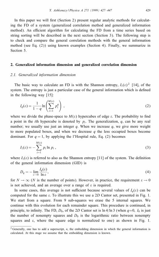
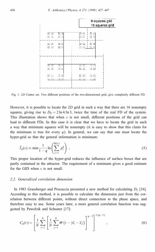
computed for the same �. To illustrate this we use a 2D Cantor set, presented in Fig. 1.We start from a square. From 9 sub-squares we erase the 5 internal squares. Wecontinue with this evolution for each remainder square. This procedure is continued, inprinciple, to in�nity. The FD, D0, of the 2D Cantor set is ln 4=ln 3 (when q=0; I0 is justthe number of nonempty squares and D0 is the logarithmic ratio between nonemptysquares and �, where the square edge is normalized to one) as shown in Fig. 1.

2 Generally, one has to add a superscript, n, the embedding dimension in which the general information iscalculated. At this stage we assume that the embedding dimension is known.


Fig. 1. 2D Cantor set. Two di�erent positions of the two-dimensional grid, give completely di�erent FD.

However, it is possible to locate the 2D grid in such a way that there are 16 nonemptysquares, giving rise to D0 = 2 ln 4=ln 3, twice the time of the real FD of the system.This illustration shows that when � is not small, di�erent positions of the grid canlead to di�erent FDs. In this case it is clear that we have to locate the grid in sucha way that minimum squares will be nonempty (it is easy to show that this claim forthe minimum is true for every q). In general, we can say that one must locate thehyper-grid so that the general information is minimum:

I q(�) ≡ min 11− q ln

(M (�)∑i=1

pqi

); (5)

This proper location of the hyper-grid reduces the in uence of surface boxes that arepartly contained in the attractor. The requirement of a minimum gives a good estimatefor the GID when � is not small.

2.2. Generalized correlation dimension

In 1983 Grassberger and Procaccia presented a new method for calculating D2 [16].According to this method, it is possible to calculate the dimension just from the cor-relation between di�erent points, without direct connection to the phase space, andtherefore easy to use. Some years later, a more general correlation function was sug-gested by Pawelzik and Schuster [17]:

Cq(r) =

1N

N∑i=1

1N

N∑j=1

�(r − |xi − xj|

)q−1

1=(q−1)

; (6)


where N is the number of points, xi is a point of the system and q is the generalizationparameter. �(x) is the Heaviside step function

�(x) ={0 when x60 ;1 when x¿ 0 :

(7)

According to this method we have to calculate the generalized probability to �nd anytwo points within a distance r. This method is some kind of integration on Eq. (2).It is not necessary to compute the real distance (e.g. ‖x‖ =

√x21 + · · ·+ x2n where n

is the phase-space dimension); it is equivalent to calculating the probability to �ndany two points in a hyper-box where one of them is located in the middle (e.g.‖x‖ = max16i6n |xi| [18]). It is easier to compute the last possibility. For the specialcase of q= 1, Eq. (6) can be written (by applying the l’Hospital’s rule [12]) as

lnC1(r) =1N

N∑i=1

ln

1N

N∑j=1

�(r − |xi − xj|) : (8)

The generalized correlation dimension (GCD) has a similar de�nition to the GID(Eq. (4)):

Dq = limN→∞;r→0

lnCq(r)ln r

: (9)

Both GID and GCD methods should give identical results. The GCD method is easyuse and gives smooth curves. On the other hand, the method requires O(N 2) compu-tations 3 . Also, the smooth curves due to averaging over all distances are associatedwith a loss in information based on the attractor structure.As we pointed out earlier, we usually have a limited number of points, forcing

us to calculate dimension at large r. Thus, an error enters the calculation of FD. Theminimum number of points needed for the FD calculation has been discussed in severalpapers and di�erent constraints suggested (for example [20,21]). In this paper we willuse the Nmin of the Eckmann and Ruelle [21] constraint:

D2¡2 log10 Nlog10(

1�); (10)

under the following conditions:

�=rr0.1; 1

2N2�D/1 (11)

with reference to the Grassberger and Procaccia method. Here, r0 is the attractor diam-eter, and r is the maximum distance that gives reliable results in Eq. (6) when q= 2.The normalized distance, �, must be small because of the misleading in uence of thehyper-surface. A � too large (close to 1) can cause incorrect results since we take

3 If one looks just at small r values, the method requires just O(N ) computations [18].


into account also hyper-boxes that are not well occupied because the major volume isoutside the attractor.However, if one has a long time series, then it is not necessary to compute all N 2

relations in Eq. (6). One can compute Eq. (6) for certain reference points such thatthe conditions in Eq. (11) will still hold. Then, Eq. (6) can be written as follows:

Cq(r) =

1Nref

Nref∑i=1

1Ndata − 2w − 1

Ndata∑j=1

�(r − |xi·s − xj|)q−1

1=(q−1)

; (12)

where

|i · s− j|¿w; s=⌊NdataNref

⌋:

For each reference point we calculate the correlation function over all data points. Thestep for the time series is s. To neglect short time correlation one must also introducea cuto�, w. Usually w ≈ m (m corresponds to the � from (1)) [22]. The number ofdistances |xi − xj| will be P = Nref(Ndata − 2w − 1) instead of N 2. The new form ofEq. (10) is

D¡log10 Plog10(

1�); (13)

and the conditions (11) become

�=rr0.1; 1

2P�D/1 : (14)

Although we discussed here a minimum number of data points needed for the dimensioncalculation, one must choose � such that the in uence from the surface is negligible(the growth of the surface is exponential to the embedding dimension). That gives usan upper limit for �. On the other hand, in order to �nd the FD we must average overa range of r, giving us a lower limit for �; therefore Nmin is determined according tothe lower limit, giving rise to larger amount of points.

3. Algorithm

3.1. Background

In this section we describe an algorithm for GID method 4 . The algorithm is basedon a string sort and can be useful both for GID and GCD methods.In previous works there have been several suggestions to compute DIG [23–28].

The key idea of some of those methods [25–27] is to rescale the coordinates of eachpoint and to express them in binary form. Then, the edge-box size can be initializedby the lowest value possible and then it doubles on each step. Those methods require

4 Computer programs are available at http:==faculty.biu.ac.il=∼ ashkenaz=FDprog=.


O(N logN ) operations. Another method [24] uses a recursive algorithm to �nd the FD.The algorithm starts from a d dimensional box which contains all data points. Then,this box is divided into 2d sub-boxes, and so on. The empty boxes are not consid-ered, and those which contain only one point are marked. This procedure requires onlyO(N ) operations (for a reasonable series length this fact does not make a signi�cantdi�erence [24]).As pointed out in Ref. [24], in spite of the e�ciency of the above algorithm (speed

and resolution), it is quite di�cult to converge to the FD of a high dimensional system.I was aware to this di�culty, and suggested a smoothing term to solve it (as will beexplained in this section). Basically, we allow any choice of edge length (in contrastto power of 2 edge size of the above methods) and optimal location of the grid issearched. This procedure leads to convergence to the FD.One of the works that calculates GID was done by Caswell and Yorke [23]. They

calculate FD of 2D maps. They have proved that it is very e�cient to divide the phasespace into circles instead of squares in spite of the neglected area between the circles.However, this approach is not suitable for higher phase-space dimensions. The reasonmight be that the volume of the hyper-balls compared to the entire volume of theattractor decreases according to the attractor dimension. In this way we lose most ofthe information that is included in the attractor, since the space between the hyper-ballsis not taken into account. It is easy to show that the ratio between the volume of thehyper-sphere with radius R, VS , and the volume of the hyper-box with edge size of2R; VB (the sphere is in the box), is

VS(2n)VB(2n)

=1

2 · 4 · 6 · · · 2n(�2

)n; (15)

for even phase space dimension, and,

VS(2n− 1)VB(2n− 1) =

11 · 3 · 5 · · · (2n− 1)

(�2

)n−1; (16)

for odd phase space dimension. It is clear that the ratios (15) and (16) tend to zerofor large n.

3.2. Algorithm

Let us call the time series x(i). The form of the reconstructed vector, Eq. (1),depends on the jumping, m, that creates the phase space. We order the time series inthe following way:

x(0); x(m); x(2m); : : : ; x((l− 1)m) ;x(1); x(1 + m); x(1 + 2m); : : : ; x(1 + (l− 1)m) ;...

x(m− 1); x(m− 1 + m); x(m− 1 + 2m); : : : ; x(m− 1 + (l− 1)m) ; (17)


where l = bNp=mc. Let us denote the new series as xi (i = 0; : : : ; (lm − 1); we loseNp − lm data points). If we take n consecutive numbers in each row, we create areconstructed vector in the n dimensional embedding dimension.At this stage, we �t a string (for each �) to the number series Eq. (17). One character

is actually a number between 0; : : : ; 255, and thus, it is possible to divide one edgeof the hyper-box to 255 parts (we need one of the 256 characters for sign). Thecorrespondence is applied in the following way. We search for the minimum value inxi series, and denote it as xmin (similarly, we denote the maximum values as xmax). Thecorresponding character to xi is

yi =⌊xi − xmin

�

⌋: (18)

The value of � is in the range

(xmax − xmin)255

6�6(xmax − xmin) : (19)

If we take now n consecutive characters (string), we have the “address” of the hyper-cube in which the corresponding vector is found.Let us represent the string as follows:

s0 = y0y1 : : : yn−1; s1 = y1 : : : yn; : : : ; sl−n = yl−n : : : yl−1 ;

sl−n+1 = yl : : : yl+n−1; : : : ; s2(l−n)+1 = y2l−n : : : y2l−1 ;

...

s(m−1)(l−n+1) = y(m−1)l : : : y(m−1)l+n−1; : : : ; sm(l−n+1)−1 = yml−n : : : yml−1 : (20)

Obviously, we do not have to keep each string si in the memory; we can keep justthe pointers to the beginning of the strings in the character series, yi. The number ofvectors=strings is m(l− n+ 1).As mentioned, each string is actually the address of a hyper-box (for which the

vector is contained) in a hyper-grid that covers the attractor. The �rst character is theposition of the �rst coordinate of the hyper-box on the �rst edge of the hyper-grid.The second character denotes the location on the second edge, and so on. We actuallygrid the attractor with a hyper-grid so that any edge in this grid can be divided into255 parts. Thus the maximal number of boxes is 255n, where n is the embeddingdimension (there is no limit for n). Most of those boxes are empty, and we keep justthe occupied boxes in the hyper-grid.The next step is to check how many vectors fall in the same box, or, in other

words, how many identical “addresses” there are. For this we have to sort the vectorthat points to strings, si, in increasing order (one string is less than the other when the�rst character that is not equal is less than the parallel character; e.g., ‘abcce’¡‘abcda’since the fourth character in the �rst string, c, is less then the fourth character in thesecond string, d). The above process is illustrated in Fig. 2.


Fig. 2. Illustration of the GID algorithm. We take series containing 12 data points between zero and one.The parameter values are: m = 3, � = 0:4 and n = 2. For simplicity, we assume that the lowest character is‘a’.

The most e�cient way to sort N elements is the “quick sort” [29] (There is other sortalgorithms that require even less computation (O(N )) such as radix sorting [30,31]).It requires just O(N log2 N ) computations. However, this sort algorithm is not suitablefor our propose, since after the vector is sorted, and we slightly increase the size ofthe edge of the hyper-box, �, there are just a few changes in the vector, and most of itremains sorted. Thus, one has to use another method which requires less computationsfor this kind of situation, because the quick sort requires O(N log2 N ) computationsindependently of the initial state. The sort that we used was a “shell sort” [29], whichrequires O(N 3=2) computations in worst case, around O(N 5=4) computations for randomseries, and O(N ) operations for an almost sorted vector. Thus, if we compute the infor-mation function for m di�erent � values O(N log2 N +mN ) operations will be needed.After sorting we count how many identical vectors there are in each box. Suppose

that we want to calculate GID for embedding dimensions nmin : : : nmax, and generaliza-tions qmin : : : qmax. We count in the sorted pointers vector identical strings containingnmax characters. Once we detect a di�erence we know that the coordinate of the boxhas changed. We detect the �rst di�erent location. A �rst di�erence in the last char-acter of the string means that it is possible to observe the di�erence just in the nthmaxembedding dimension, and in lower embedding dimension it is impossible to observethe di�erence. If the �rst mismatch is in the nth character in the string, then the boxchanges for embedding dimensions higher than or equal to n. We hold a counter vector


for the di�erent embedding dimensions, and we will assign zero for those embeddingdimensions in which we observed a change. At this stage, we have to add to the resultsmatrix the probability to fall in a box according to Eqs. (2), (3). We continue withthis method to the end of the pointer vector and then print the results matrix for thecurrent � and continue to the next �.It is easy to show that one does not have to worry about the range of the generaliza-

tion, q, because for large time series with 106 data points the range of computationalq’s is from −100 to 100.The method of string sorting can be used also for calculating GCD. Our algorithm

is actually a generalization of the method that was suggested by Grassberger [18].The algorithm is specially e�cient for small r (r ¡ (1=10)D where D is the attractordiameter) and it requires O(N log2 N ) computations instead of O(N

2) computations(according to the Grassberger algorithm it requires O(N ) computations instead O(N 2)computations).The basic idea of Grassberger was that for small rmax values, where rmax is the

maximum distance for which the correlation function is computed, one does not haveto consider distances larger than rmax, distances which require most of the computationtime. Thus, it is enough to consider just the neighboring boxes (we use the de�nitiondistance ‖x‖ = max16i6n |xi| in Eq. (6)), for which their edge is equal to rmax, sincedistances greater than rmax are not considered in Eq. (6). If, for example, one wantsto calculate the correlation of r6rmax = (1=10)D (in accordance with conditions (10)(11) (13) (14)), then (in 2D projection) it is enough to calculate distances in 9 squaresinstead 100 squares (actually, it is enough to consider just 5 squares since Eq. (6) issymmetric). According to Grassberger, one has to build a matrix in which any cellpoints to the list of data points located in it. It is possible to generalize this methodto a 3D projection matrix.The generalization to higher dimensions can be done very easily according to the

string sort method. As a �rst step one has to prepare a string yi (18), which is thesame operation as gridding the attractor by a hyper-grid of size r. The next step is tosort strings si (20). For each reference point in Eq. (12) the boxes adjoining the boxwith the reference point in it should be found. Now, it is left to �nd the distancesbetween the reference point to other points in neighboring boxes (we keep the pointervector from string yi to the initial series and vice versa), and calculate the correlationaccording to Eq. (12).The algorithm described above is especially e�cient for very complex systems with

high FD. For example, for EEG series produced by brain activity, it is well known(except for very special cases such as epilepsy [19]) that the FD is, at least, four.In this case nmin = 4, and instead of calculating distances in l4 boxes (l is the ratiobetween the attractor diameter and r) it is su�cient to calculate distances in 34 = 81boxes. If, for example, l = 9, just 34=94 = 1=81 distances must be computed (or evenless if one takes into account also the symmetry of Eq. (12)). In this way, despitethe O(N log2 N ) operations needed for the initial sort, one can reduce signi�cantly thecomputation time.


3.3. Testing of GID algorithm and number of data points needed for calculatingGID

Let us test the algorithm of GID on random numbers. We create a random seriesbetween 0 to 1 (uniform distribution). We then reconstruct the phase-space accordingto Takens theory (1). For any embedding dimension that we would like to reconstruct,the phase space we will get a dimension that is the same as the embedding dimension,since the new reconstructed vectors are random in the new phase space, and hence �llthe space (in our case, a hypercube of edge 1).For embedding dimension 1 (a simple line), if the edge length is �, then the proba-

bility to fall on any edge is also �. The number of edges � that covers the series range[0; 1) is b1=�c. The probability to fall on the last edge is (1mod �) (the residue of thedivision). For generalization q one gets

M (�)∑i=1

pqi = b1=�c�q + (1mod �)q : (21)

For embedding dimension 2, one has to square (21) since the probability distributionon di�erent sides is equal. For embedding dimension n Eq. (2) becomes

Iq(�) =1

1− q ln[b1=�c�q + (1mod �)q]n : (22)

Opening Eq. (22) according to the binomial formula will give all di�erent combinationsfor the partly contained boxes. Notice that this grid location ful�lls requirement (5)for the minimum information function.In Fig. 3 we present −I2(�), both, according to the GID algorithm, and according

to Eq. (22). There is full correspondence between the curves, and, as we �nd, it ispossible to see that the slope (dimension) in the embedding dimension n is equal to thedimension itself. When −I2(�) ≈ −10, the curves separate. There is lower convergence(when −I2(�) ≈ −12:5) since the edge is too small, and the number of reconstructedvectors is equal to the number of nonempty boxes.The “saw tooth” that is seen in Fig. 3 is caused by partial boxes that fall on the

edge of the hyper-box. The “saw tooth” appears when there is an integer number ofedges that covers the big edge. The slope in the beginning of every saw tooth is equalto zero (that comes from the extremum condition of (22)). The “saw teeth” becomesmaller when � decrease, since the relative number of boxes that fall on the surface insmall compared to the entire number of boxes.It is possible to calculate roughly the number of points needed for the dimen-

sion calculation in a homogeneous system. The separation point of Fig. 3 is approx-imately around −I2(�) ≈ −10, for every embedding dimension. Thus, the number ofhyper-boxes at this point is e10 (since −10 = ln(M (�)p2) where p ∼ 1=M (�) in ourexample). The graph comes to a saturation around −I2(�) ≈ −12:5, giving rise to e12:5data points. The number of points per box is just, e2:5 ≈ 12. Thus, generally, whenthere are less then 12 points per box, the value of Iq(�) is unreliable. Let us denote the


Fig. 3. Dimension calculation for random series by GID algorithm and by the theory.

minimum edges needed for the calculation as mmin (mmin is just b1=�c, and thus onecan de�ne a lower value for �). The number of hyper-boxes in embedding dimensionn is mnmin. Thus, the minimum number of points needed for computing the FD of anattractor with an FD D, is

N = 12mDmin : (23)

This estimate is less than what was required by Smith [20] (42D) and larger then therequirement of Eckmann and Ruelle [21] (if we take, for example, mmin = 1=� = 10then according to Eq. (10), 10D=2 points is needed and according to Eq. (23), 12×10Dpoints is needed). However, as we pointed out earlier, Eq. (23) is a rough estimation,and one can converge to a desired FD even with less points.

4. Examples

In this section we will present the results of both GID and GCD on well-knownsystems, such as the Lorenz attractor and the Rossler attractor. The FD of those re-sults are well known by various methods, and we will present almost identical resultsachieved by our methods. In the following examples, we choose one of the coordinatesto be the time series; we normalize the time series to be in the range of 0; : : : ; 1.

4.1. Lorenz attractor

The Lorenz attractor [32] is represented by a set of three �rst-order non-lineardi�erential equations:

dxdt= �(y − x) ;


dydt=−xz + rx − y ;

dzdt= xy − bz : (24)

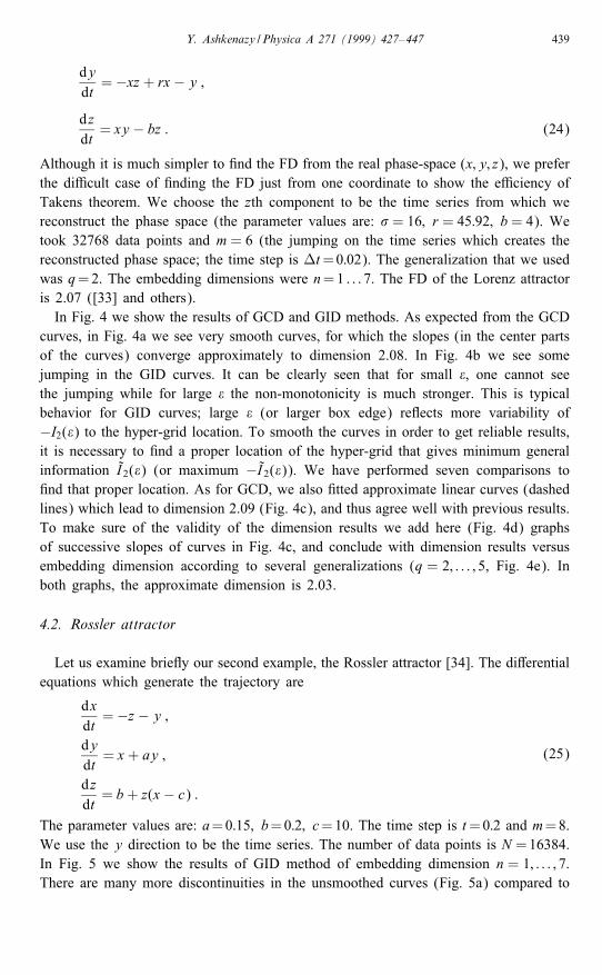
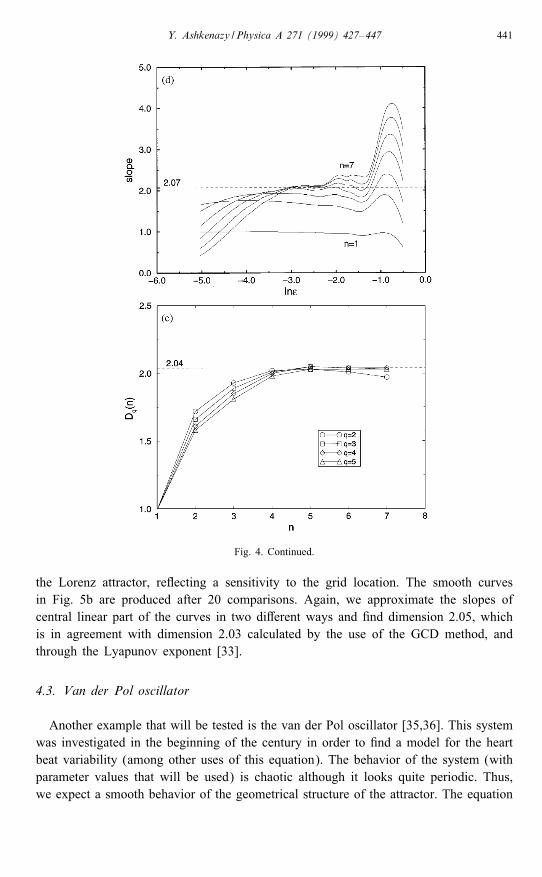
Although it is much simpler to �nd the FD from the real phase-space (x; y; z), we preferthe di�cult case of �nding the FD just from one coordinate to show the e�ciency ofTakens theorem. We choose the zth component to be the time series from which wereconstruct the phase space (the parameter values are: � = 16; r = 45:92; b = 4). Wetook 32768 data points and m = 6 (the jumping on the time series which creates thereconstructed phase space; the time step is �t=0:02). The generalization that we usedwas q=2. The embedding dimensions were n=1 : : : 7. The FD of the Lorenz attractoris 2.07 ([33] and others).In Fig. 4 we show the results of GCD and GID methods. As expected from the GCD

curves, in Fig. 4a we see very smooth curves, for which the slopes (in the center partsof the curves) converge approximately to dimension 2.08. In Fig. 4b we see somejumping in the GID curves. It can be clearly seen that for small �, one cannot seethe jumping while for large � the non-monotonicity is much stronger. This is typicalbehavior for GID curves; large � (or larger box edge) re ects more variability of−I2(�) to the hyper-grid location. To smooth the curves in order to get reliable results,it is necessary to �nd a proper location of the hyper-grid that gives minimum generalinformation I 2(�) (or maximum −I 2(�)). We have performed seven comparisons to�nd that proper location. As for GCD, we also �tted approximate linear curves (dashedlines) which lead to dimension 2.09 (Fig. 4c), and thus agree well with previous results.To make sure of the validity of the dimension results we add here (Fig. 4d) graphsof successive slopes of curves in Fig. 4c, and conclude with dimension results versusembedding dimension according to several generalizations (q = 2; : : : ; 5, Fig. 4e). Inboth graphs, the approximate dimension is 2.03.

4.2. Rossler attractor

Let us examine brie y our second example, the Rossler attractor [34]. The di�erentialequations which generate the trajectory are

dxdt=−z − y ;

dydt= x + ay ;

dzdt= b+ z(x − c) :

(25)

The parameter values are: a=0:15; b=0:2; c=10. The time step is t=0:2 and m=8.We use the y direction to be the time series. The number of data points is N =16384.In Fig. 5 we show the results of GID method of embedding dimension n = 1; : : : ; 7.There are many more discontinuities in the unsmoothed curves (Fig. 5a) compared to


Fig. 4. Correlation and information curves of reconstructed Lorenz attractor. (a) Correlation curves; the esti-mate slopes are added. (b) Unsmoothed information curves. (c) Smoothed information curves; the estimatedlinear curves (dashed line) and their slope is added. (d) The slopes of −I2(�) (Fig. 4c). The dashed linerepresents the estimated FD. (e) FD of Lorenz attractor for di�erent embedding dimensions, n, and fordi�erent generalizations, q.


Fig. 4. Continued.

the Lorenz attractor, re ecting a sensitivity to the grid location. The smooth curvesin Fig. 5b are produced after 20 comparisons. Again, we approximate the slopes ofcentral linear part of the curves in two di�erent ways and �nd dimension 2.05, whichis in agreement with dimension 2.03 calculated by the use of the GCD method, andthrough the Lyapunov exponent [33].

4.3. Van der Pol oscillator

Another example that will be tested is the van der Pol oscillator [35,36]. This systemwas investigated in the beginning of the century in order to �nd a model for the heartbeat variability (among other uses of this equation). The behavior of the system (withparameter values that will be used) is chaotic although it looks quite periodic. Thus,we expect a smooth behavior of the geometrical structure of the attractor. The equation


Fig. 5. (a) Unsmoothed graphs of Rossler attractor. (b) Smoothed information graphs; the FD estimation isadded.

of motion is

�x − �(1− x2)x + kx = f cost : (26)

The parameter values are: = 2:446, � = 5, k = 1 and f = 1. Habib and Ryne [37]and others [38] have found that the Lyapunov exponents of the system are �1 ≈ 0:098,�2 = 0 and �3 ≈ −6:84, and thus, according to the Kaplan and Yorke formula [1],

DL = j +∑j

i=1 �i|�j+1| ≈ 2 + 0:098

6:84≈ 2:014 ; (27)

where j is de�ned by the condition that∑j

i=1 �i ¿ 0 and∑j+1

i=1 �i ¡ 0. The fact thatthe system has a “periodic” nature is re ected in this very low FD (as known, theminimal FD of a chaotic system is 2).


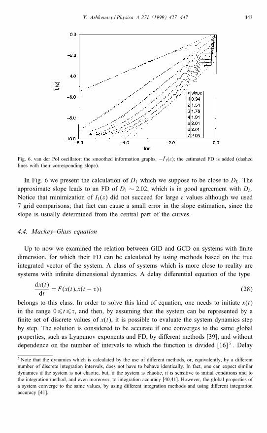
Fig. 6. van der Pol oscillator: the smoothed information graphs, −I1(�); the estimated FD is added (dashedlines with their corresponding slope).

In Fig. 6 we present the calculation of D1 which we suppose to be close to DL. Theapproximate slope leads to an FD of D1 ∼ 2:02, which is in good agreement with DL.Notice that minimization of I1(�) did not succeed for large � values although we used7 grid comparisons; that fact can cause a small error in the slope estimation, since theslope is usually determined from the central part of the curves.

4.4. Mackey–Glass equation

Up to now we examined the relation between GID and GCD on systems with �nitedimension, for which their FD can be calculated by using methods based on the trueintegrated vector of the system. A class of systems which is more close to reality aresystems with in�nite dimensional dynamics. A delay di�erential equation of the type

dx(t)dt

= F(x(t); x(t − �)) (28)

belongs to this class. In order to solve this kind of equation, one needs to initiate x(t)in the range 06t6�, and then, by assuming that the system can be represented by a�nite set of discrete values of x(t), it is possible to evaluate the system dynamics stepby step. The solution is considered to be accurate if one converges to the same globalproperties, such as Lyapunov exponents and FD, by di�erent methods [39], and withoutdependence on the number of intervals to which the function is divided [16] 5 . Delay

5 Note that the dynamics which is calculated by the use of di�erent methods, or, equivalently, by a di�erentnumber of discrete integration intervals, does not have to behave identically. In fact, one can expect similardynamics if the system is not chaotic, but, if the system is chaotic, it is sensitive to initial conditions and tothe integration method, and even moreover, to integration accuracy [40,41]. However, the global properties ofa system converge to the same values, by using di�erent integration methods and using di�erent integrationaccuracy [41].


Fig. 7. Mackey–Glass equation: (a) The GCD graphs. One notices two regions of parallel curves, whichlead to di�erent FDs. (b) The successive slopes of a. (c) The GID graphs. (d) The successive slopes of c.

equations, such as Eq. (28), describe systems in which a stimulus has a delay response.There are many practical examples from control theory, economics, population biology,and other �elds.One of the known examples is the model of blood cell production in patients with

leukemia, formulated by Mackey and Glass [42]:

x(t) =ax(t − �)

1 + [x(t − �)]c − bx(t) : (29)

Following Refs. [16,39], the parameter values are: a=0:1, b=0:2, and c=10. We con�neourselves to �= 30:0. As in Ref. [16], we choose the time series to be {x(t); x(t + �);


Fig. 7. Continued.

x(t+2�); : : :}, 6 as well as the integration method which is described in this reference.The length of the time series is N = 131072.The FD (D2) calculation of the Mackey–Glass equation is presented in Fig. 7. The

embedding dimensions are, n = 1; : : : ; 9. In Fig. 7a, the correlation function, C2(r) isshown. One notices that there are two regions in each one of which there is convergenceto a certain slope. These regions are separated by a dashed line. In Fig. 7b, the averagelocal slope of Fig. 7a is shown. One can identify easily two convergences, the �rst

6 In fact, the common procedure of reconstructing a phase space from a time series is described in Eq. (1).According to this method, one has to build the reconstructed vectors by the use of a jumping choice mwhich is determined by the �rst zero of the autocorrelation function, or the �rst minimum of the mutualinformation function [8]. However, we used the same series as in Ref. [16] in order to compare results.


in the neighborhood of ∼ 3:0, and the second around ∼ 2:4. Thus, there are twoapproximations for the FD, D2, pointing to two di�erent scales. The �rst approximationis similar to the FD that was calculated in Ref. [16]. However, the GID graphs whichare presented in Fig. 7c and 7d lead to an FD, D2 ∼ 2:45, which seems to be veryclose to the second convergence of Fig. 7b. Notice that the convergence to D2 ∼ 2:4appears, in both methods, in the neighborhood of the same box size (∼ 2:1).

5. Summary

In this work we develop a new algorithm for calculation of a general type of infor-mation, Iq(n), which is based on string sorting (the method of string sort can be usedalso to calculate the conventional GCD method). According to our algorithm, one candivide the phase space into 255 parts in each hyper-box edge. The algorithm requiresO(N log2 N ) computations, where N is the number of reconstructed vectors. A roughestimate for the number of points needed for the FD calculation was given. The algo-rithm, which can be used in a regular system with known equations of motion, wastested on a reconstructed phase space (which was built according to Takens theorem).The general information graphs have non-monotonic curves, which can be smoothedby the requirement for minimum general information. We examine our algorithm onsome well known examples, such as, the Lorenz attractor, the Rossler attractor, the vander Pol oscillator and others, and show that the FD that was computed by the GIDmethod is almost identical to the well-known FDs of those systems.In practice, the computation time of an FD using the GID method, was much less

than for the GCD method. For a typical time series with 32768 data points, the com-putation time needed for the GCD method was about nine times greater than thecomputation time of GID method (when we do not restrict ourselves to small r valuesand we compute all N 2 relations). Thus, in addition to the fact that the algorithmdeveloped in this paper enables the use of comparative methods (which is crucial insome cases), the algorithm is generally faster.

Acknowledgements

The author wishes to thank J. Levitan, M. Lewkowicz and L.P. Horwitz for veryuseful discussions.

References

[1] J.L. Kaplan, J.A. Yorke, in: H.-O. Peitgen, H.-O. Walther (Eds.), Functional Di�erential Equations andApproximations of Fixed Points, Lecture Notes in Mathematics 730, Springer, Berlin, 1979.

[2] A. Babloyantz, C. Nicolis, M. Salazar, Phys. Rev. A 111 (1985) 152.[3] A. Babloyantz, A. Destexhe, Proc. Nat. Acad. Sci. USA 83 (1986) 3513.[4] E. Basar (Ed.), Chaos in the Brain, Springer, Berlin, 1990.


[5] G. Mayer-Kress, F.E. Yates, L. Benton, M. Keidel, W.S. Tirsch, S.J. Poepple, Math. Biosci. 90 (1988)155.

[6] K. Saermark, J. Lebech, C.K. Bak, A. Sabers, in: E. Basar, T.H. Bullock (Eds.), Springer Series inBrain Dynamics, Springer, Berlin, 1989, p. 149.

[7] K. Saermark, Y. Ashkenazy, J. Levitan, M. Lewkowicz, Physica A 236 (1997) 363.[8] F. Takens, in: D. Rand, L.S. Young (Eds.), Dynamical Systems and Turbulence, Springer, Berlin, 1981.[9] H.G. Schuster, Deterministic Chaos, Physik Verlag, Weinheim, 1989.[10] A.M. Fraser, H.L. Swinney, Phys. Rev. A 33 (1986) 1134.[11] J.-C. Roux, R.H. Simoyi, H.L. Swinney, Physica D 8 (1983) 257.[12] H.D.I. Abarbanel, R. Brown, J.J. Sidorowich, L.S. Tsimring, Rev. Mod. Phys. 65 (1993) 1331.[13] M. Ding, C. Grebobi, E. Ott, T. Sauer, J.A. Yorke, Physica D 8 (1993) 257.[14] C.E. Shannon, W. Weaver, The Mathematical Theory of Information, University of ll Press, Urbana,

1949.[15] J. Balatoni, A. Reny, in: P. Turan (Ed.), Selected Papers of A. Renyi, Akademiai K. Budapest, 1976,

588 p.[16] P. Grassberger, I. Procaccia, Physica D 9 (1983) 189.[17] K. Pawelzik, H.G. Schuster, Phys. Rev. A 35 (1987) 481.[18] P. Grassberger, Phys. Lett. A 148 (1990) 63.[19] A. Babloyantz, A. Destexhe, in: M. Markus, S. Muller, G. Nicolis (Eds.), From Chemical to Biological

Organization, Springer, Berlin, 1988.[20] L.A. Smith, Phys. Lett. A 133 (1988) 283.[21] J.-P. Eckmann, D. Ruelle, Physica D 56 (1992) 185.[22] J. Theiler, Phys. Rev. A 34 (1986) 2427.[23] W.E. Caswell, J.A. York, in: G. Mayer-Kress (Ed.), Dimensions and Entropies in Chaotic Systems,

Springer, Berlin, 1986.[24] T.C.A. Molteno, Phys. Rev. E 48 (1993) 3263.[25] X.-J. Hou, R. Gilmore, G. Mindlin, H. Solari, Phys. Lett. A 151 (1990) 43.[26] A. Block, W. von Bloh, H. Schnellnhuber, Phys. Rev. A 42 (1990) 1869.[27] L. Liebovitch, T. Toth, Phys. Lett. A 141 (1989) 386.[28] A. Kruger, Comp. Phys. Commun. 98 (1996) 224.[29] W.H. Press, S.A. Teukolsky, W.T. Vetterling, B.P. Flannery, Numerical Recipes in C, 2nd Edition,

Cambridge University Press, Cambridge, 1995.[30] D.E. Knooth, The Art of Computer Programming, Vol. 3 – Sorting and Searching, Addison-Wesley,

Reading, MA, 1975.[31] A.V. Aho, J.E. Hopcroft, J.D. Ullman, Data Structures and Algorithms, Addison-Wesley, MA, 1983.[32] E.N. Lorenz, J. Atmos. Sci. 20 (1963) 130.[33] A. Wolf, J.B. Swift, H.L. Swinney, J.A. Vastano, Physica D 16 (1985) 285.[34] O.E. Rossler, Phys. Lett. 57A (1976) 397.[35] B. van der Pol, Philos. Mag. (7) 2 (1926) 978.[36] B. van der Pol, van der Mark, Philos. Mag. (7) 6 (1928) 763.[37] S. Habib, R.D. Ryne, Phys. Rev. Lett. 74 (1995) 70.[38] K. Geist, U. Parlitz, W. Lauterborn, Prog. Theor. Phys. 83 (1990) 875.[39] J.D. Farmer, Physica D 4 (1981) 366.[40] J.M. Greene, J. Math. Phys. 20 (1979) 1183.[41] Y. Ashkenazy, C. Goren, L.P. Horwitz, Phys. Lett. A 243 (1998) 195.[42] M.C. Mackey, L. Glass, Science 197 (1977) 287.

The use of generalized information dimension in measuring fractal dimension of time series

Documents

Transcript of The use of generalized information dimension in measuring fractal dimension of time series