Scalar Minimizers with Fractal Singular Sets
14
ARMA manuscript No. (will be inserted by the editor) Scalar minimizers with fractal singular sets Irene Fonseca, Jan Mal´ y, Giuseppe Mingione Abstract Lack of regularity of local minimizers for convex functionals with non- standard growth conditions is considered. It is shown that for every ε> 0 there exists a function a ∈ C α (Ω) such that the functional F : u 7→ Z Ω (|Du| p + a(x)|Du| q ) dx admits a local minimizer u ∈ W 1,p (Ω) whose set of non-Lebesgue points is a closed set Σ with dim H (Σ) >N - p - ε, and where 1 <p<N<N + α< q< +∞. Key words. Gap, non standard growth conditions, regularity, Hausdorff dimension Mathematics Subject Classification (2000): 35J20, 35E99, 49J45, 74G40 1. Introduction The aim of this paper is to present an example of a convex regular integral in the Calculus of Variations which admits a minimizer with a very wild singular set. The striking features of the example are that the problem is scalar and the Hausdorff dimension of the singular set is quite big; in fact, the set of non-Lebesgue points is of Cantor type. We consider the functional F : u 7→ Z Ω f (x, Du) dx , u ∈ W 1,p (Ω), (1) where Ω ⊂ R N is a bounded domain and f : Ω × R N → R is a non-negative Carath´ eodory function.
-
Upload
independent -
Category
Documents
-
view
2 -
download
0
Transcript of Scalar Minimizers with Fractal Singular Sets

ARMA manuscript No.(will be inserted by the editor)
Scalar minimizers with fractal singular sets
Irene Fonseca, Jan Maly, Giuseppe Mingione
Abstract
Lack of regularity of local minimizers for convex functionals with non-standard growth conditions is considered. It is shown that for every ε > 0there exists a function a ∈ Cα(Ω) such that the functional
F : u 7→∫
Ω
(|Du|p + a(x)|Du|q) dx
admits a local minimizer u ∈ W 1,p(Ω) whose set of non-Lebesgue points isa closed set Σ with dimH(Σ) > N −p−ε, and where 1 < p < N < N +α <q < +∞.
Key words. Gap, non standard growth conditions, regularity, Hausdorffdimension
Mathematics Subject Classification (2000): 35J20, 35E99, 49J45, 74G40
1. Introduction
The aim of this paper is to present an example of a convex regularintegral in the Calculus of Variations which admits a minimizer with a verywild singular set. The striking features of the example are that the problemis scalar and the Hausdorff dimension of the singular set is quite big; in fact,the set of non-Lebesgue points is of Cantor type.
We consider the functional
F : u 7→∫
Ω
f(x,Du) dx , u ∈ W 1,p(Ω), (1)
where Ω ⊂ RN is a bounded domain and f : Ω×RN → R is a non-negativeCaratheodory function.

2 Irene Fonseca, Jan Maly, Giuseppe Mingione
A classical result due to Giaquinta & Giusti ([GG]), resting on DeGiorgi’s iteration method ([DG1]), states that any local minimizer u ∈W 1,p(Ω) of a functional of type (1) satisfying, for some p > 1 and 1 <L < +∞, the growth assumptions
L−1|ξ|p − L ≤ f(x, ξ) ≤ L(|ξ|p + 1), x ∈ Ω, ξ ∈ RN , (2)
is locally Holder continuous. This result holds true even without any con-vexity assumption on f . Observe that this is not the case in the vectorialsetting u : Ω → Rk , k > 1 (see for instance the counterexamples in [DG2],[N], [SY1], [SY2]). If the functional does not meet the condition (2), butsatisfies only the more flexible (p, q)-growth conditions (following the ter-minology introduced by Marcellini in [M2])
L−1|ξ|p − L ≤ f(x, ξ) ≤ L(|ξ|q + 1), 1 ≤ L, 1 < p < q < +∞, (3)
then the continuity of minimizers generally fails, provided p and q are notnear enough, as shown by counterexamples (see [Gia], [H], [M1], [M2]).In particular, in the paper [M2], Marcellini presents a minimizer of an au-tonomous functional within the structure (3) exhibiting a singular set whichis a line. In [M3] he raised the question of finding a minimizer of a regularfunctional (that is, with f being a Holder or Lipschitz continuous function)with an isolated singularity. This problem was solved in a sharp way in[ELM]. All these examples require that the ratio q/p is not very close to 1.Indeed, in [ELM] it was shown that if f(·, ξ) is Holder continuous with anexponent α ∈ (0, 1], then a sufficient condition for a minimizer (which, bydefinition, is a priori only in W 1,p
loc (Ω)) to be in W 1,qloc (Ω) is that
q
p< 1 +
α
N. (4)
This condition is sharp, as proved in [ELM], what shows that for this typeof functionals the regularity of minimizers depends on a subtle interplaybetween the size of the ratio q/p and the regularity of f(x, ξ) with respectto the variable x.
In what follows, we will be particularly interested on functionals of type(1) of the form
f(x, ξ) = |ξ|p + a(x)|ξ|q, a(x) ≥ 0.
In this setting it is possible to conctruct examples of singular minimizers offunctionals with coefficients having a cone type singularity. In the two di-mensional case, Zhikov [Z] constructed an example exhibiting the Lavrentievphenomenon. A similar geometry has been used in [ELM] to produce sharpexamples of minimizers with isolated singularities in arbitrary dimension.This is the starting point of this paper where, based on the construction in[ELM] and via an iterative process, we build local minimizers having fractalsingular sets.

Scalar minimizers with fractal singular sets 3
Since until now all known examples provided singularities which wereeither isolated or concentrated on a line, we found it natural to ask how“bad” the singular set of a minimizer of a functional with (p, q) growth canbe. Our aim is to show that under natural assumptions (that is, as soon asthe sufficient condition for regularity in (4) is violated) minimizers may havevery wild singular sets of Cantor type, with Hausdorff dimension “touching”the borderline case. Indeed, we have
Theorem 1. For every choice of the parameters:
2 ≤ N , α ∈ (0, +∞) , 1 < p < N < N + α < q < +∞ , ε > 0 ,(5)
there exist a functional
F : u 7→∫
Ω
(|Du|p + a(x)|Du|q) dx, u ∈ W 1,p(Ω), (6)
with Ω ⊂ RN being a bounded Lipschitz domain, a ∈ Cα(Ω), a ≥ 0, a localminimizer u ∈ W 1,p(Ω) of F and a closed set Σ ⊂ Ω with
dimH(Σ) > N − p− ε
such that all the points of Σ are non-Lebesgue points of the precise repre-sentative of u.
In the previous statement, and using standard notation, Cα denotes thespace of all functions with continuous derivatives up to the order [α] (theinteger part of α, whereas α := α − [α] is the noninteger part of α),with the [α]-th derivative being α-Holder continuous. We use the symboldimH(A) for the Hausdorff dimension of a set A ⊂ RN .
Observe that the results of the previous theorem are sharp in more thanone respect. Indeed, the choice of the parameters made in (5) is necessary(at least when α ∈ (0, 1]) in order to violate the condition (4). Moreover,because u is a Sobolev function in W 1,p(Ω), the Hausdorff dimension of thesingular set cannot exceed N −p, and here we can reach N −p− ε for everyε > 0, while all the counterexamples presented up to now exhibited singularsets of dimension at most 1. Note that from condition (6) it follows that themore we want the integrand function f to be smooth the more we need pand q to be far apart. Furthermore, the Hausdorff dimension of the singularset Σ does not depend on the choice of the parameters α and q (but, ofcourse, it does depend on N , p and ε). Finally, if we allow the function fto be only Holder continuous with respect to x, then we can ensure that uis regular outside Σ, in the sense that u ∈ W 1,q
loc (Ω \Σ). Precisely,
Theorem 2. For every choice of the parameters
2 ≤ N , α ∈ (0, 1) , 1 < p < N < N + α < q <(1 +
1N
)p , ε > 0 ,

4 Irene Fonseca, Jan Maly, Giuseppe Mingione
there exist a functional
F : u 7→∫
Ω
(|Du|p + a(x)|Du|q) dx , u ∈ W 1,p(Ω),
with Ω ⊂ RN being a bounded Lipschitz domain, a ∈ Cα(Ω), a ≥ 0, a localminimizer u ∈ W 1,p(Ω) of F and a closed set Σ ⊂ Ω with
dimH(Σ) > N − p− ε,
such that all the points of Σ are non-Lebesgue points of the precise repre-sentative of u. Moreover,
u ∈ W 1,qloc (Ω \Σ),
and, in particular, the function u is continuous at every point of Ω \Σ.
2. Preliminaries
Recall that a function u ∈ W 1,1loc (Ω) is said to be a local minimizer of a
functional F of type (6) if∫
supp (u−v)
f(x,Du) dx ≤∫
supp (u−v)
f(x,Dv) dx
for every function v ∈ W 1,1loc (Ω) with supp (u− v) ⊂ Ω.
We will use the following result from [ELM, Theorem 5.1]
Theorem 3. Let u ∈ W 1,ploc (Ω) be a local minimizer of the functional
u 7→∫
Ω
(|Du|p + a(x)|Du|q) dx, u ∈ W 1,ploc (Ω) ,
where a ∈ Lip(Ω), a ≥ 0. Suppose that the exponents 1 < p < q < +∞, aresuch that
q
p< 1 +
1N
.
Thenu ∈ W 1,q
loc (Ω).
We say that u is precisely represented if
u(x) = limr→0+
1|B(x, r)|
∫
B(x,r)
u(y) dy
whenever the limit on the right exists.In what follows, C denotes a generic constant which may vary from
expression to expression.

Scalar minimizers with fractal singular sets 5
3. Construction
3.1. Underlying geometry
We will work in the space RN , and we set
K0 = (−1, 1)N , V = −1, 1N−1 × 0.We will construct sequences of sets and functions on the unit cube K0. Fixa parameter λ ∈ (0, 1/2) and use the powers λn as radii in our construction.We define inductively a countable family of finite sets Zn ⊂ (−1, 1)N−1 ×0, for n = 0, 1, 2, . . . , whose elements will be used as centers for cubes inour construction. We start by letting
Z0 := 0RN .Let n ∈ N and suppose that we have constructed Zk for k = 0, . . . , n − 1.Define
Zzn := z + λnV : V ∈ V, z ∈ RN , n ∈ N ,
Zn :=⋃
z∈Zn−1
Zzn.
Since Zk ∩ Zn = ∅ for k < n, without any ambiguity and in order tosimplify the notation, we will use often z ∈ Zn also as a subscript, andthe information about the integer n under consideration will be implicitlycontained in the symbol z. We set
Kz := z + (−λn, λn)N ,
K ′z := z + (−2λn+1, 2λn+1)N−1 × (−λn+1, λn+1).
If z ∈ Zn then we consider in each cube Kz a concentric block K ′z which
we split into 2N−1 cubes Kz′ , z′ ∈ Zzn+1.
For any x ∈ Kz we write
φz(x) := max
λn+1, 1−λ1−2λ
∣∣x− z∣∣∞ − λn+1
1−2λ
,
where we denote by z the projection of z onto (−1, 1)N−1, i.e. z :=(z1, . . . , zN−1), and∣∣x∣∣
∞ := max|x1|, |x2|, ..., |xk| , for x = (x1, x2, ..., xk) ∈ Rk, k ∈ N .
Now, we partition each cube Kz into the “p-domain” Pz and the “q-domain”Qz, precisely
Pz := x ∈ Kz : |xN | < φz(x),Q+
z := x ∈ Kz : xN > φz(x),Q−
z := x ∈ Kz : −xN > φz(x),Qz := Q+
z ∪Q−z .
6 Irene Fonseca, Jan Maly, Giuseppe Mingione
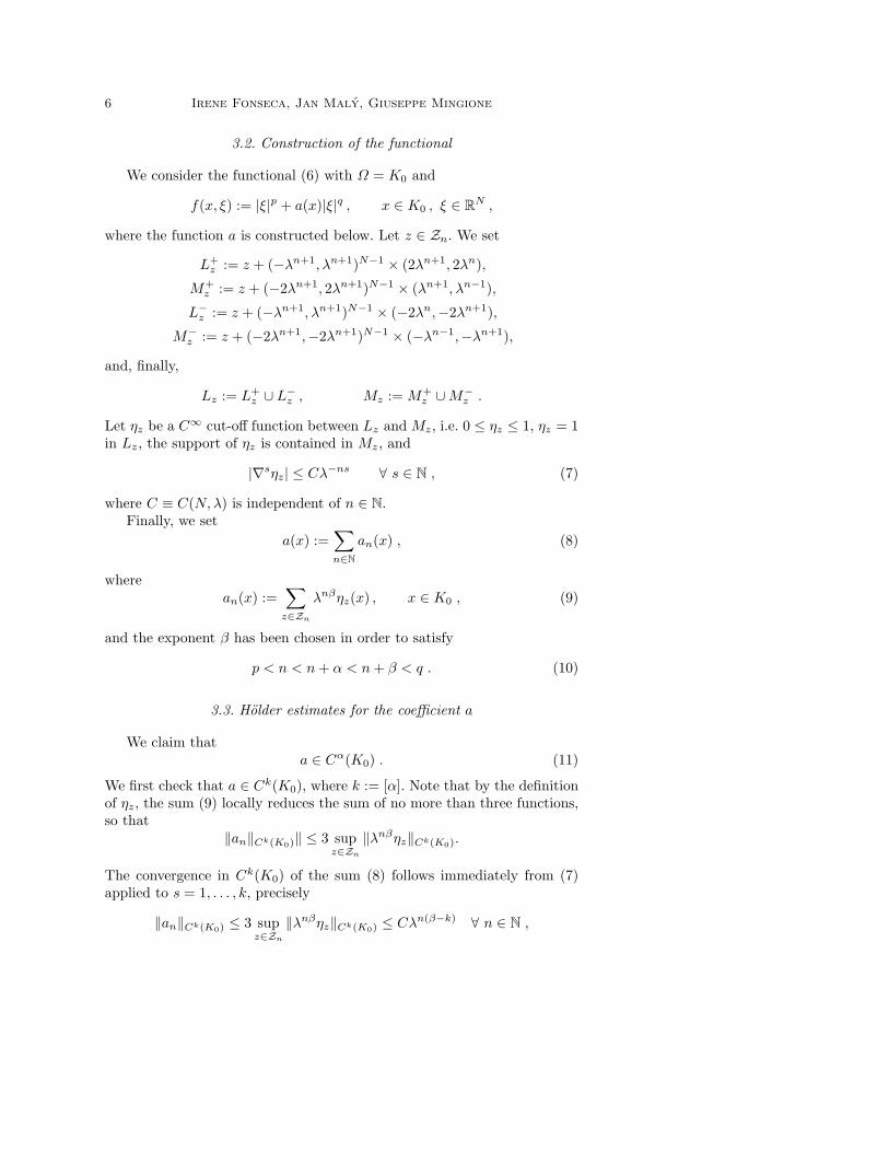
3.2. Construction of the functional
We consider the functional (6) with Ω = K0 and
f(x, ξ) := |ξ|p + a(x)|ξ|q , x ∈ K0 , ξ ∈ RN ,
where the function a is constructed below. Let z ∈ Zn. We set
L+z := z + (−λn+1, λn+1)N−1 × (2λn+1, 2λn),
M+z := z + (−2λn+1, 2λn+1)N−1 × (λn+1, λn−1),
L−z := z + (−λn+1, λn+1)N−1 × (−2λn,−2λn+1),
M−z := z + (−2λn+1,−2λn+1)N−1 × (−λn−1,−λn+1),
and, finally,
Lz := L+z ∪ L−z , Mz := M+
z ∪M−z .
Let ηz be a C∞ cut-off function between Lz and Mz, i.e. 0 ≤ ηz ≤ 1, ηz = 1in Lz, the support of ηz is contained in Mz, and
|∇sηz| ≤ Cλ−ns ∀ s ∈ N , (7)
where C ≡ C(N,λ) is independent of n ∈ N.Finally, we set
a(x) :=∑
n∈Nan(x) , (8)
wherean(x) :=
∑
z∈Zn
λnβηz(x) , x ∈ K0 , (9)
and the exponent β has been chosen in order to satisfy
p < n < n + α < n + β < q . (10)
3.3. Holder estimates for the coefficient a
We claim thata ∈ Cα(K0) . (11)
We first check that a ∈ Ck(K0), where k := [α]. Note that by the definitionof ηz, the sum (9) locally reduces the sum of no more than three functions,so that
‖an‖Ck(K0)‖ ≤ 3 supz∈Zn
‖λnβηz‖Ck(K0).
The convergence in Ck(K0) of the sum (8) follows immediately from (7)applied to s = 1, . . . , k, precisely
‖an‖Ck(K0) ≤ 3 supz∈Zn
‖λnβηz‖Ck(K0) ≤ Cλn(β−k) ∀ n ∈ N ,

Scalar minimizers with fractal singular sets 7
(recall that, owing to (10), it holds β − k > 0).Now, we must prove that ∇ka is Holder continuous with exponent α.
For any x, y ∈ K0, we have
|∇ka(x)−∇ka(y)| ≤∑
n∈N
∑
z∈Zn
λnβ |∇kηz(x)−∇kηz(y)| , (12)
where, arguing as before, there are at most six non-vanishing terms in thesum (12). Therefore, it suffices to prove that there exists an absolute con-stant such that for every z ∈ Zn, n ∈ N,
λnβ |∇kηz(x)−∇kηz(y)| ≤ C|x− y|α .
We distinguish two cases. If |x− y| ≤ λn then, using the Mean Value The-orem and (7) with s = k + 1, we have
λnβ |∇kηz(x)−∇kηz(y)| ≤ λnα|∇kηz(x)−∇kηz(y)|≤ λnα||∇(k+1)ηz||∞|x− y|= λnα||∇(k+1)ηz||∞|x− y|1−α|x− y|α≤ Cλnαλ−n(k+1)|x− y|1−α|x− y|α≤ C|x− y|α .
If |x− y| > λn, then, using (7) with s = k, we obtain
λnβ |∇kηz(x)−∇kηz(y)| ≤ 2λnα||∇(k)ηz||∞≤ 2Cλn(α−k)
≤ 2C|x− y|α ,
where C is the absolute constant appearing in (7). The proof of (11) is nowcomplete.
3.4. Low energy competitor
We construct recursively a sequence of functions unn∈N. First we set
u0(x) :=
xN
φ0(x) if x ∈ P0,
1 if x ∈ Q+0 ,
−1 if x ∈ Q−0 .
For a general n ∈ N, and assuming that u1, u2, ..., un−1 have been deter-mined, we define the corrector function cz as
cz(x) :=
xN
φz(x) if x ∈ Pz,
1 if x ∈ Q+z ,
−1 if x ∈ Q−z .
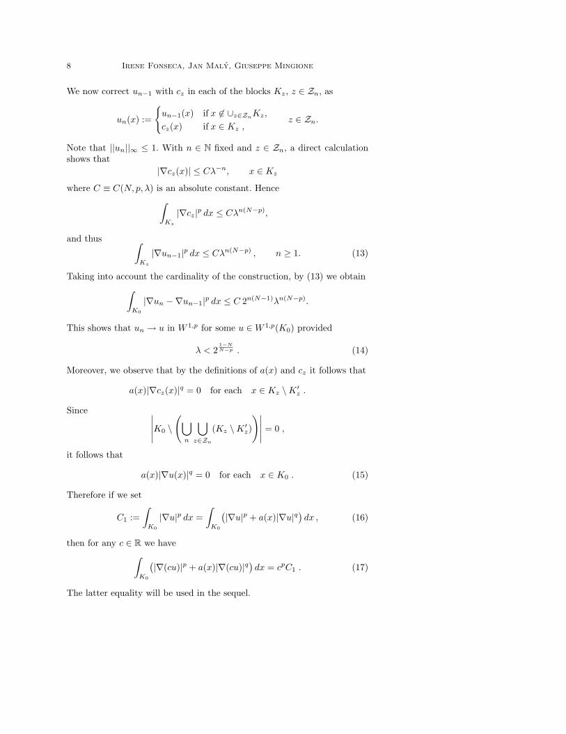
8 Irene Fonseca, Jan Maly, Giuseppe Mingione
We now correct un−1 with cz in each of the blocks Kz, z ∈ Zn, as
un(x) :=
un−1(x) if x 6∈ ∪z∈Zn
Kz,
cz(x) if x ∈ Kz ,z ∈ Zn.
Note that ||un||∞ ≤ 1. With n ∈ N fixed and z ∈ Zn, a direct calculationshows that
|∇cz(x)| ≤ Cλ−n, x ∈ Kz
where C ≡ C(N, p, λ) is an absolute constant. Hence∫
Kz
|∇cz|p dx ≤ Cλn(N−p),
and thus ∫
Kz
|∇un−1|p dx ≤ Cλn(N−p) , n ≥ 1. (13)
Taking into account the cardinality of the construction, by (13) we obtain∫
K0
|∇un −∇un−1|p dx ≤ C 2n(N−1)λn(N−p).
This shows that un → u in W 1,p for some u ∈ W 1,p(K0) provided
λ < 21−NN−p . (14)
Moreover, we observe that by the definitions of a(x) and cz it follows that
a(x)|∇cz(x)|q = 0 for each x ∈ Kz \K ′z .
Since ∣∣∣∣∣K0 \(⋃
n
⋃
z∈Zn
(Kz \K ′z)
)∣∣∣∣∣ = 0 ,
it follows that
a(x)|∇u(x)|q = 0 for each x ∈ K0 . (15)
Therefore if we set
C1 :=∫
K0
|∇u|p dx =∫
K0
(|∇u|p + a(x)|∇u|q) dx , (16)
then for any c ∈ R we have∫
K0
(|∇(cu)|p + a(x)|∇(cu)|q) dx = cpC1 . (17)
The latter equality will be used in the sequel.
Scalar minimizers with fractal singular sets 9
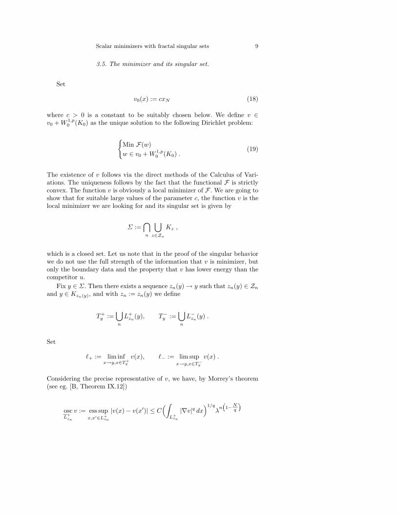
3.5. The minimizer and its singular set.
Set
v0(x) := cxN (18)
where c > 0 is a constant to be suitably chosen below. We define v ∈v0 + W 1,p
0 (K0) as the unique solution to the following Dirichlet problem:
Min F(w)w ∈ v0 + W 1,p
0 (K0) .(19)
The existence of v follows via the direct methods of the Calculus of Vari-ations. The uniqueness follows by the fact that the functional F is strictlyconvex. The function v is obviously a local minimizer of F . We are going toshow that for suitable large values of the parameter c, the function v is thelocal minimizer we are looking for and its singular set is given by
Σ :=⋂n
⋃
z∈Zn
Kz ,
which is a closed set. Let us note that in the proof of the singular behaviorwe do not use the full strength of the information that v is minimizer, butonly the boundary data and the property that v has lower energy than thecompetitor u.
Fix y ∈ Σ. Then there exists a sequence zn(y) → y such that zn(y) ∈ Zn
and y ∈ Kzn(y), and with zn := zn(y) we define
T+y :=
⋃n
L+zn
(y), T−y :=⋃n
L−zn(y) .
Set
`+ := lim infx→y,x∈T+
y
v(x), `− := lim supx→y,x∈T−y
v(x) .
Considering the precise representative of v, we have, by Morrey’s theorem(see eg. [B, Theorem IX.12])
oscL
+zn
v := ess supx,x′∈L+
zn
|v(x)− v(x′)| ≤ C(∫
L+zn
|∇v|q dx)1/q
λn1−N
q
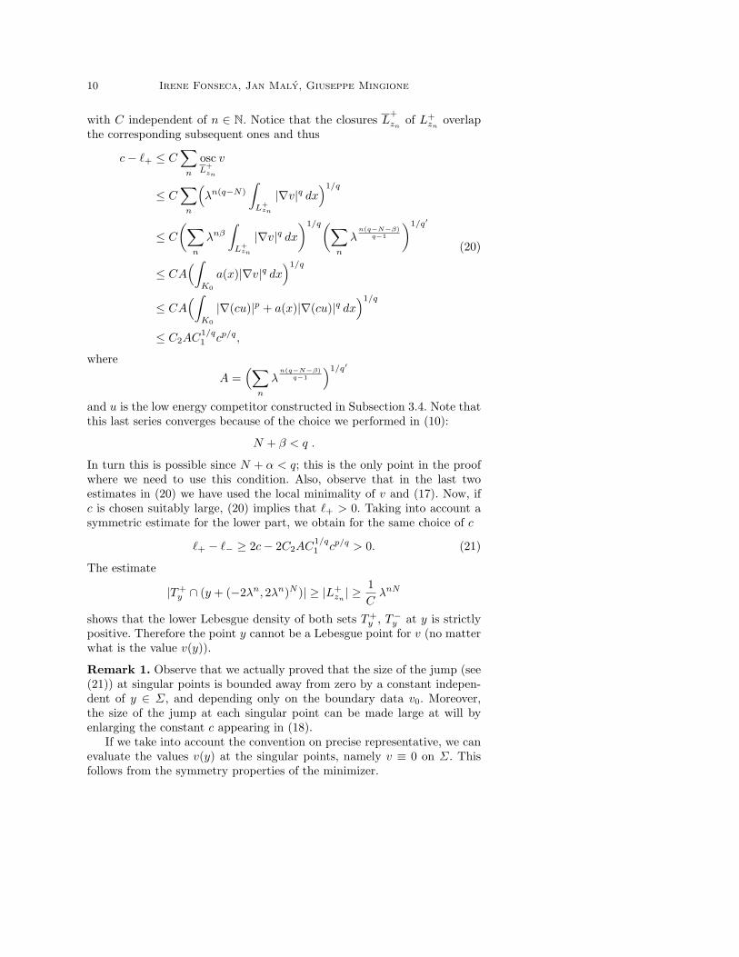
10 Irene Fonseca, Jan Maly, Giuseppe Mingione
with C independent of n ∈ N. Notice that the closures L+
znof L+
znoverlap
the corresponding subsequent ones and thus
c− `+ ≤ C∑
n
oscL
+zn
v
≤ C∑
n
(λn(q−N)
∫
L+zn
|∇v|q dx)1/q
≤ C
(∑n
λnβ
∫
L+zn
|∇v|q dx
)1/q(∑n
λn(q−N−β)
q−1
)1/q′
≤ CA(∫
K0
a(x)|∇v|q dx)1/q
≤ CA(∫
K0
|∇(cu)|p + a(x)|∇(cu)|q dx)1/q
≤ C2AC1/q1 cp/q,
(20)
where
A =(∑
n
λn(q−N−β)
q−1
)1/q′
and u is the low energy competitor constructed in Subsection 3.4. Note thatthis last series converges because of the choice we performed in (10):
N + β < q .
In turn this is possible since N + α < q; this is the only point in the proofwhere we need to use this condition. Also, observe that in the last twoestimates in (20) we have used the local minimality of v and (17). Now, ifc is chosen suitably large, (20) implies that `+ > 0. Taking into account asymmetric estimate for the lower part, we obtain for the same choice of c
`+ − `− ≥ 2c− 2C2AC1/q1 cp/q > 0. (21)
The estimate
|T+y ∩ (y + (−2λn, 2λn)N )| ≥ |L+
zn| ≥ 1
CλnN
shows that the lower Lebesgue density of both sets T+y , T−y at y is strictly
positive. Therefore the point y cannot be a Lebesgue point for v (no matterwhat is the value v(y)).
Remark 1. Observe that we actually proved that the size of the jump (see(21)) at singular points is bounded away from zero by a constant indepen-dent of y ∈ Σ, and depending only on the boundary data v0. Moreover,the size of the jump at each singular point can be made large at will byenlarging the constant c appearing in (18).
If we take into account the convention on precise representative, we canevaluate the values v(y) at the singular points, namely v ≡ 0 on Σ. Thisfollows from the symmetry properties of the minimizer.
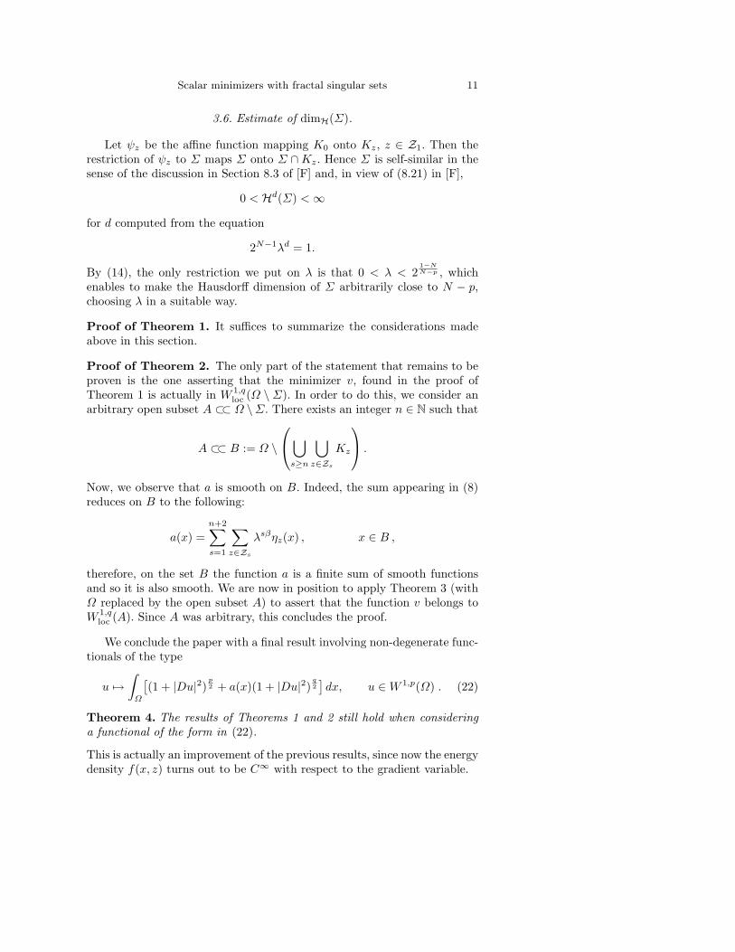
Scalar minimizers with fractal singular sets 11
3.6. Estimate of dimH(Σ).
Let ψz be the affine function mapping K0 onto Kz, z ∈ Z1. Then therestriction of ψz to Σ maps Σ onto Σ ∩Kz. Hence Σ is self-similar in thesense of the discussion in Section 8.3 of [F] and, in view of (8.21) in [F],
0 < Hd(Σ) < ∞for d computed from the equation
2N−1λd = 1.
By (14), the only restriction we put on λ is that 0 < λ < 21−NN−p , which
enables to make the Hausdorff dimension of Σ arbitrarily close to N − p,choosing λ in a suitable way.
Proof of Theorem 1. It suffices to summarize the considerations madeabove in this section.
Proof of Theorem 2. The only part of the statement that remains to beproven is the one asserting that the minimizer v, found in the proof ofTheorem 1 is actually in W 1,q
loc (Ω \ Σ). In order to do this, we consider anarbitrary open subset A ⊂⊂ Ω \Σ. There exists an integer n ∈ N such that
A ⊂⊂ B := Ω \ ⋃
s≥n
⋃
z∈Zs
Kz
.
Now, we observe that a is smooth on B. Indeed, the sum appearing in (8)reduces on B to the following:
a(x) =n+2∑s=1
∑
z∈Zs
λsβηz(x) , x ∈ B ,
therefore, on the set B the function a is a finite sum of smooth functionsand so it is also smooth. We are now in position to apply Theorem 3 (withΩ replaced by the open subset A) to assert that the function v belongs toW 1,q
loc (A). Since A was arbitrary, this concludes the proof.
We conclude the paper with a final result involving non-degenerate func-tionals of the type
u 7→∫
Ω
[(1 + |Du|2) p
2 + a(x)(1 + |Du|2) q2]dx, u ∈ W 1,p(Ω) . (22)
Theorem 4. The results of Theorems 1 and 2 still hold when consideringa functional of the form in (22).
This is actually an improvement of the previous results, since now the energydensity f(x, z) turns out to be C∞ with respect to the gradient variable.
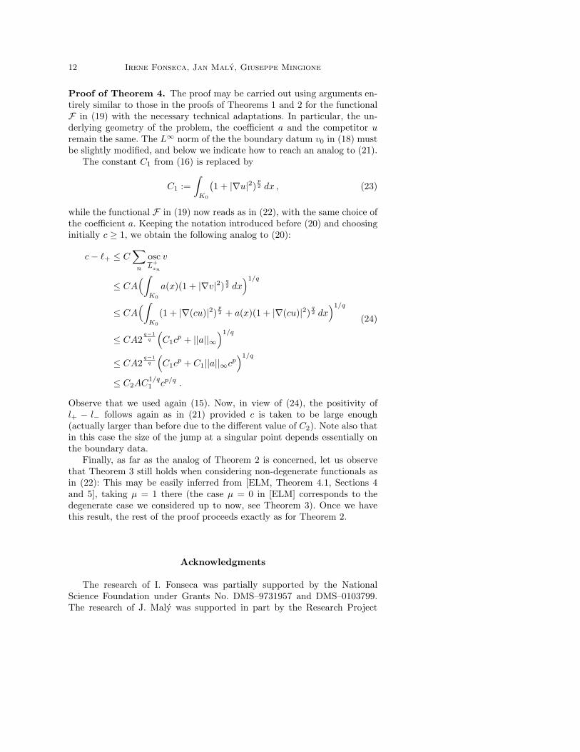
12 Irene Fonseca, Jan Maly, Giuseppe Mingione
Proof of Theorem 4. The proof may be carried out using arguments en-tirely similar to those in the proofs of Theorems 1 and 2 for the functionalF in (19) with the necessary technical adaptations. In particular, the un-derlying geometry of the problem, the coefficient a and the competitor uremain the same. The L∞ norm of the the boundary datum v0 in (18) mustbe slightly modified, and below we indicate how to reach an analog to (21).
The constant C1 from (16) is replaced by
C1 :=∫
K0
(1 + |∇u|2) p
2 dx , (23)
while the functional F in (19) now reads as in (22), with the same choice ofthe coefficient a. Keeping the notation introduced before (20) and choosinginitially c ≥ 1, we obtain the following analog to (20):
c− `+ ≤ C∑
n
oscL
+zn
v
≤ CA(∫
K0
a(x)(1 + |∇v|2) q2 dx
)1/q
≤ CA(∫
K0
(1 + |∇(cu)|2) p2 + a(x)(1 + |∇(cu)|2) q
2 dx)1/q
≤ CA2q−1
q
(C1c
p + ||a||∞)1/q
≤ CA2q−1
q
(C1c
p + C1||a||∞cp)1/q
≤ C2AC1/q1 cp/q .
(24)
Observe that we used again (15). Now, in view of (24), the positivity ofl+ − l− follows again as in (21) provided c is taken to be large enough(actually larger than before due to the different value of C2). Note also thatin this case the size of the jump at a singular point depends essentially onthe boundary data.
Finally, as far as the analog of Theorem 2 is concerned, let us observethat Theorem 3 still holds when considering non-degenerate functionals asin (22): This may be easily inferred from [ELM, Theorem 4.1, Sections 4and 5], taking µ = 1 there (the case µ = 0 in [ELM] corresponds to thedegenerate case we considered up to now, see Theorem 3). Once we havethis result, the rest of the proof proceeds exactly as for Theorem 2.
Acknowledgments
The research of I. Fonseca was partially supported by the NationalScience Foundation under Grants No. DMS–9731957 and DMS–0103799.The research of J. Maly was supported in part by the Research Project
Scalar minimizers with fractal singular sets 13
MSM 113200007 from the Czech Ministry of Education, and by Grant No.201/03/0931 from the Grant Agency of the Czech republic (GA CR). Theresearch of G. Mingione was funded by MIUR under the project “Calcolodelle Variazioni” (Cofin 2002).
Part of this work was undertaken when J. Maly and G. Mingione werevisiting the Center for Nonlinear Analysis (NSF Grant No. DMS–9803791),Carnegie Mellon University, Pittsburgh, PA, USA, and when J. Maly wasvisiting the Department of Mathematics of the University of Parma. Wethank these institutions for their support during the preparation of thispaper.
The authors are indebted to the referee for his/her very careful read-ing of the manuscript and many useful comments and suggestions whichsignificantly improved the paper.
References
[B] Brezis, H., Analyse Fonctionnelle, Masson, 1983.[DG1] De Giorgi, E., Sulla differenziabilita e l’analiticita delle estremali degli
integrali multipli regolari, Mem. Accad. Sci. Torino. Cl. Sci. Fis. Mat.Nat. (3) 3 (1957), 25-43.
[DG2] De Giorgi, E., Un esempio di estremali discontinue per un problema vari-azionale di tipo ellittico, Boll. Un. Mat. Ital. (4) 1 (1968), 135-137.
[ELM] Esposito, L., Leonetti, F. & Mingione, G., Sharp regularity for functionalswith (p, q) growth, J. Differential Equations, to appear.
[F] Falconer, K. J., The Geometry of Fractal Sets, Cambridge Tracts in Math.Press, 1985.
[Gia] Giaquinta, M., Growth conditions and regularity, a counterexample,Manuscripta Math. 59 (1987), 245-248.
[GG] Giaquinta, M. & Giusti, E., On the regularity of the minima of variationalintegrals, Acta Math. 148 (1982), 31-46.
[H] Hong, M. C., Some remarks on the minimizers of variational integrals withnonstandard growth conditions, Boll. Un. Mat. Ital. A (7) 6 (1992), 91-101.
[M1] Marcellini, P., Un example de solution discontinue d’un probleme varia-tionnel dans le cas scalaire, Preprint, No. 11. Istituto Matematico U. Dini,Universita di Firenze, 1987-1988.
[M2] Marcellini, P., Regularity and existence of solutions of elliptic equationswith p, q-growth conditions, J. Differential Equations 90 (1991), 1–30.
[M3] Marcellini, P., Regularity for elliptic equations with general growth condi-tions, J. Differential Equations 105 (1993), 296-333.
[N] Necas, J., Example of an irregular solution to a nonlinear elliptic systemwith analytic coefficients and conditions for regularity, Theory of nonlinearoperators (Proc. Fourth Internat. Summer School, Acad. Sci., Berlin, 1975,197–206.
[SY1] Sverak, V. & Yan, X., A singular minimizer of a smooth strongly convexfunctional in three dimensions, Calc. Var. Partial Differential Equations10 (2000), 213–221.
[SY2] Sverak, V. & Yan, X., Non Lipschitz minimizers of smooth uniformly con-vex variational integrals, Proc. Nat. Acad. Sci. USA 99 (24) (2002), 15269–15276.
[Z] Zhikov, V. V., On Lavrentiev’s phenomenon (Russian), J. Math. Physics3 (1995), 249–269.

14 Irene Fonseca, Jan Maly, Giuseppe Mingione
Department of Mathematical SciencesCarnegie Mellon University
Pittsburgh, PA 15213-3890, [email protected];
and
Department of Mathematical AnalysisFaculty of Mathematics and Physics
Charles UniversitySokolovska 83, 186 75 Praha 8, Czech Republic
and
Department of MathematicsUniversity of Parma
via M. D’Azeglio 85/a, 43100 Parma, [email protected].