
QUANTUM GRAVITY EFFECTS IN SCALAR, VECTOR AND ...
118
QUANTUM GRAVITY EFFECTS IN SCALAR, VECTOR AND TENSOR FIELD PROPAGATION ANINDITA DUTTA Bachelor of Science, West Bengal State University, 2012 Master of Science, RKM Vivekananda University, 2014 A Thesis Submitted to the School of Graduate Studies of the University of Lethbridge in Partial Fulfillment of the Requirements for the Degree MASTER OF SCIENCE Department of Physics and Astronomy University of Lethbridge LETHBRIDGE, ALBERTA, CANADA c Anindita Dutta, 2016
-
Upload
khangminh22 -
Category
Documents
-
view
0 -
download
0
Transcript of QUANTUM GRAVITY EFFECTS IN SCALAR, VECTOR AND ...
QUANTUM GRAVITY EFFECTS IN SCALAR, VECTOR AND TENSOR FIELDPROPAGATION
ANINDITA DUTTABachelor of Science, West Bengal State University, 2012Master of Science, RKM Vivekananda University, 2014
A ThesisSubmitted to the School of Graduate Studies
of the University of Lethbridgein Partial Fulfillment of the
Requirements for the Degree
MASTER OF SCIENCE
Department of Physics and AstronomyUniversity of Lethbridge
LETHBRIDGE, ALBERTA, CANADA
c© Anindita Dutta, 2016

QUANTUM GRAVITY EFFECTS IN SCALAR, VECTOR AND TENSOR FIELDPROPAGATION
ANINDITA DUTTA
Date of Defense: December 12, 2016
Dr. Arundhati DasguptaSupervisor Associate Professor Ph.D.
Dr. Ken VosCommittee Member Associate Professor Ph.D.
Dr. Stacey WetmoreCommittee Member Professor Ph.D.
Dr. Viqar HusainExternal Committee Member Professor Ph.D.
Dr. Mark WaltonChair, Thesis Examination Com-mittee
Professor Ph.D.

Dedication
To my Parents
for supporting me all the way.
And to my Teachers who made me who I am.
iii

Abstract
Quantum theory of gravity deals with the physics of the gravitational field at Planck length
scale (10−35 m). Even though it is experimentally hard to reach the Planck length scale, one
can look for evidence of quantum gravity that is detectable in astrophysics. In this thesis,
we try to find effects of loop quantum gravity corrections on observable phenomena. We
show that the quantum fluctuation strain for LIGO data would be 10−125 on the Earth. The
correction is, however, substantial near the black hole horizon. We discuss the effect of this
for scalar field propagation followed by vector and tensor fields. For the scalar field, the
correction introduces a new asymmetry; for the vector field, we found a new perturbation
solution and for the tensor field, we found the corrected Einstein equations which are yet
to solve. These will affect phenomena like Hawking radiation, black hole entropy and
gravitational waves.
iv

Acknowledgments
I would like to thank my supervisor Dr. Arundhati Dasgupta for her kind support and
encouragement during this Master’s project. Her positive outlook and confidence in my re-
search inspired me and gave me confidence. I am also grateful to my supervisory committee
members, especially to Dr. Ken Vos and Prof. Viqar Husain. They were very generous with
their time and knowledge, and assisted me in each step to complete this thesis.
My sincere thanks to the School of Graduate Studies at University of Lethbridge for
giving me this opportunity and funding me during my research. I would also like to thank all
the students and the members of Department of Physics and Astronomy for their friendship
and help.
This journey would not be possible without the support from my family. I am grateful
to them for their encouragement and kind words when I needed it. My special thanks goes
to my friend Partha Paul for helping me with Mathematica and proof reading of this thesis.
I am also thankful to my teachers, especially to Dr. Ashik Iqubal, for advising me on the
numerical set-up required in this project. To my friends from Lethbridge and roommates,
thank you for listening, offering me advice, and supporting me through this entire process.
v

Contents
Contents vi
Lists of Abbreviations, Consants and Symbols viii
List of Figures xi
1 Introduction 11.1 This Thesis . . . . . . . . . . . . . . . . . . . . . . . . . . . . . . . . . . 71.2 Outline . . . . . . . . . . . . . . . . . . . . . . . . . . . . . . . . . . . . 91.3 Notations and Representation . . . . . . . . . . . . . . . . . . . . . . . . . 10
1.3.1 General Notations . . . . . . . . . . . . . . . . . . . . . . . . . . 101.3.2 Coordinate System . . . . . . . . . . . . . . . . . . . . . . . . . . 11
2 Classical Gravity 132.1 Special Theory of Relativity . . . . . . . . . . . . . . . . . . . . . . . . . 142.2 Riemannian Geometry and Einstein’s Field Equation . . . . . . . . . . . . 202.3 Scalar, Vector and Tensor Fields . . . . . . . . . . . . . . . . . . . . . . . 322.4 Schwarzschild Solution . . . . . . . . . . . . . . . . . . . . . . . . . . . . 342.5 Conclusion . . . . . . . . . . . . . . . . . . . . . . . . . . . . . . . . . . 38
3 Canonical Quantum Gravity and The Semi-classical Correction 393.1 Hamiltonian Formulation of General Relativity . . . . . . . . . . . . . . . 413.2 Ashtekar Variables and Loop Quantum Gravity . . . . . . . . . . . . . . . 503.3 Kinematical Coherent States in Loop Quantum Gravity . . . . . . . . . . . 563.4 Semi-classical Correction in Schwarzschild Space-time: New Result . . . . 59
3.4.1 Static and Spherical Metrics . . . . . . . . . . . . . . . . . . . . . 623.4.2 Non-static Space-time . . . . . . . . . . . . . . . . . . . . . . . . 633.4.3 Non-spherical Space-time . . . . . . . . . . . . . . . . . . . . . . 633.4.4 The Strain . . . . . . . . . . . . . . . . . . . . . . . . . . . . . . . 64
3.5 Conclusion . . . . . . . . . . . . . . . . . . . . . . . . . . . . . . . . . . 65
4 Effect on The Scalar Field 664.1 Corrected Scalar Field Evolution . . . . . . . . . . . . . . . . . . . . . . . 674.2 Numerical Solution: New Result . . . . . . . . . . . . . . . . . . . . . . . 704.3 Conclusion . . . . . . . . . . . . . . . . . . . . . . . . . . . . . . . . . . 75
vi

CONTENTS
5 Effect on The Vector Field 775.1 Electromagnetic Field in Curved Space-Time . . . . . . . . . . . . . . . . 785.2 Electromagnetic Field Propagation in Schwarzschild Background . . . . . . 805.3 Electromagnetic Field Propagation in Corrected Schwarzschild Black Hole:
New Result . . . . . . . . . . . . . . . . . . . . . . . . . . . . . . . . . . 835.4 Conclusion . . . . . . . . . . . . . . . . . . . . . . . . . . . . . . . . . . 89
6 Conclusion 906.1 Work in Progress: Effect on Gravitational Wave in Corrected Black Hole
Background . . . . . . . . . . . . . . . . . . . . . . . . . . . . . . . . . . 91
Bibliography 95
A RNPL Pogramming for Numerical Solution 104
vii

Lists of Abbreviations, Consants andSymbols
List of Abbreviations
ADM metric Arnowitt, Deser and Misner metricCMB Cosmic Microwave BackgroundCODATA Committee on Data for Science and TechnologyEHT Event Horizon TelescopeeV electron-VoltGPS Global Positioning SystemLHS Left Hand SideLIGO Laser Interferometer Gravitational-Wave ObservatoryRHS Right Hand SideRNPL Rapid Numerical Prototyping Language
List of Constants
ε0 = 8.854×10⁻¹² m−3Kg−1S4A2 ........Permittivity of the free space~= 6.626×10⁻³⁴ m2kg/s ........Planck constantµ0 = 1.256×10⁻⁶ H/m ........Permeability of the free spacec = 2.99×10⁸/m/s ........Speed of light in a vacuum inertial frameG = 6.674×10⁻¹¹ m3kg−1s−2 ........Gravitational constantlp = 1.62×10⁻³⁵ m ........Planck length
List of Symbols
∗F IJµν Dual of the curvature F IJ
µν
i, j, k Euclidean basis vectors in 3dLn Lie derivative along vector nµ
M Four dimensional manifoldΠ Canonical momentum conjugate to NΠa Canonical momentum conjugate to Na
Πab Canonical momentum conjugate to qab
ℜ Real partΣ Constant time three dimensional hypersurface
viii

LISTS OF ABBREVIATIONS, CONSANTS AND SYMBOLS
d’Alembertian operatorβ Immirzi parameterAµ Four vector potentialAIJ
µ Spin connectionDa Covariant derivative defined on Σ
e EdgeEI TriadeI
µ TetradF IJ
µν Curvature due to spin connectionH Hamiltonian densityhe(A) HolonomyKµν Extrinsic curvatureKab Extrinsic curvature of Σ
L Lagrangian densityN Lapse functionNµ Shift vectorPI
e Momentum corresponding to holonomyPl(cosθ) Legendre polynomial of order lqµν Projector onto Σ
qab Metric tensor on Σ
R(3)µνρσ Three Riemann curvature
R(3) Three Ricci scalarR(3)
µν Three Ricci tensorrg Schwarzschild radiusr∗ Tortoise coordinateYlm Spherical harmonicsB Magnetic fieldE Electric fieldηµν Minkowski metric tensorΓλ
µν Affine connectioneµ Basis vectorΛ
µν Lorentz transformation matrix
J Current density∇µ Covariant derivative⊗ Direct product∂µ
∂
∂xµ
ρ Charge densityτP Tangent space of the point Pϕ Scalar fieldξ : M→ N ξ maps the elements of M to the elements of Nξ−1 : N→M Inverse mapping between the sets M and NCp Continuous and p-times differentiable mapdr, dθ, dφ Infinitesimal Space coordinates in spherical polar coordinate systemdt Infinitesimal time coordinate
ix

CONTENTS
dx, dy, dz Infinitesimal space coordinates in Cartesian coordinate systemFµν Antisymmetric electromagnetic fieldg Determinant of the metric tensorGµν Einstein tensorgµν Metric tensor in curved space-timeM Mass of the black holeR Ricci scalarr, θ, φ Space coordinates in spherical polar coordinate systemRn n-dimensional Euclidean spaceRµ
νρσ Riemann curvatureRµν Ricci tensorS ActionSn n-dimensional spheret Time coordinateT µν Stress-energy tensorT i1i2...im
j1 j2... jn Tensor of rank (m,n)uµ Four velocityx, y, z Space coordinates in Cartesian coordinate systemxµ Contravariant vectorxµ Covariant vectorGreek indices run from 0 to 3Latin indices run from 1 to 3
x

List of Figures
1.1 Gravitational wave strain from a binary black hole system . . . . . . . . . . 31.2 Pictorial view of the Gravitational Lensing . . . . . . . . . . . . . . . . . . 41.3 Time dilation in the clocks for a GPS . . . . . . . . . . . . . . . . . . . . . 51.4 Cartesian coordinate system . . . . . . . . . . . . . . . . . . . . . . . . . 111.5 Spherical coordinate system . . . . . . . . . . . . . . . . . . . . . . . . . 11
2.1 Light cone for an event . . . . . . . . . . . . . . . . . . . . . . . . . . . . 172.2 Parallel transport of a vector on a two sphere . . . . . . . . . . . . . . . . . 262.3 Commutator of covariant derivatives . . . . . . . . . . . . . . . . . . . . . 28
3.1 Edge intersecting surface S . . . . . . . . . . . . . . . . . . . . . . . . . . 553.2 An SU(2) coherent state . . . . . . . . . . . . . . . . . . . . . . . . . . . . 58
4.1 Plotting of the scalar field potential ϕ vs. x without correction . . . . . . . . 724.2 Plotting of the scalar field potential ϕ vs. x with twist term β = x2(x−1)2 . 744.3 Plotting of scalar field potential ϕ vs. x with twist term β = sin2(x2(x−1)2) 75
5.1 A(r) vs. r for λ = 0 . . . . . . . . . . . . . . . . . . . . . . . . . . . . . . 88
xi

Chapter 1
Introduction
If I have seen
further than others,
it is by standing upon
the shoulders of giants.
– Isaac Newton
One of the most important discoveries in the history of science is the existence of grav-
ity. Sir Isaac Newton (1642−1727), an English mathematician and physicist, realized that
there must be a force between the Earth and a falling object and this force causes the object
to accelerate towards the Earth. This insight resulted in the universal law of gravitation,
“ Every object in the universe attracts every other object with a force directly proportional
to the product of their masses and inversely proportional to the square of the distance be-
tween the centres of them” [1]. This proportionality turns into an equation with the help of a
proportionality constant namely gravitational constant denoted as G. The value of this con-
stant was derived later by Henry Cavendish (1798) and it is G = 6.754× 10⁻¹¹N.m2/kg2
(The value of G recommended by CODATA in 2014 is 6.674×10⁻¹¹N.m2/kg2 ) [2].
Newton’s laws have achieved many successes in explaining orbital rotations in our so-
lar system, although it could not accurately explain the perihelion precession in the orbital
motion of Mercury [3]. Later, this problem was resolved by Albert Einstein’s ‘General
Theory of Relativity’ in 1915 [4]. Einstein’s theory defines gravity as a result of space-
1

1. INTRODUCTION
time curvature. According to this theory, space and time are on the same footing, hence
interchangeable. Although Einstein’s gravity treats space and time very differently com-
pared to Newtonian theory, general theory of relativity is able to explain everything that
Newton’s theory did as well as some natural phenomena that would not be justified by
Newton’s theory, e.g. bending of light and perihelion precession of Mercury [1].
One of the most important consequence of the general theory of relativity is the Black
Hole [1]. A black hole is a region of space with very high gravity from which not even
light can escape. It can be formed from the death of a massive star with sufficiently large
mass or from primordial density fluctuations. The general theory of relativity predicts the
space-time structure of a black hole and also explains the physics behind it. Direct detection
of a black hole is quite challenging as it does not emit any detectable radiation. However,
there is indirect evidence that confirms the existence of black holes [5]. Later in this thesis,
we will explain the black hole more elaborately.
Another surprising outcome of the general theory of relativity is the existence of Grav-
itational Waves, which are basically ripples caused by a moving massive object in the
space-time curvature. The gravitational wave propagates in free space with the speed of
light. As the gravitational effect is very weak compared to other physical forces (G ∼
O(10−11) N m2/kg2), it is a difficult task to get experimental evidence of a gravitational
wave. Even though the existence of the gravitational wave was predicted by Einstein around
1916-1918 [6], it took almost 100 years to get experimental evidence of the wave. After
a long period of constant effort and breathless waiting, in 2016, LIGO finally announced
the experimental detection of gravitational waves [7]. This discovery not only opened a
new window for research, but also set the standards for precision, by detecting an effect in
space-time of order 10−21. The first received gravitation wave data, as detected by LIGO,
provide us the mass of the source black hole which was created by merging two black holes.
They received a strain of order 10−21 as shown in Figure 1.1. The data also predicted the
distance of the event from the Earth as well as the approximate radius of the source black
2

1. INTRODUCTION
Figure 1.1: Gravitational wave strain from a binary black hole system [7].
hole [7].
Along with these consequences, general theory of relativity also has applications in
observational astronomy, modern cosmology and GPS of the Earth [9]. Gravitational
lensing is one of the important tools in observational astronomy [10]. According to the
general theory of relativity, if there is a strong gravity source between the observer and
a distant target object in space, then light coming from the object will bend around the
gravity source. As a result, the observer sees multiple distorted images of the object as
shown in Figure 1.2. In the figure, D is a high gravity source lying between the observer
and the target object S. Lights coming from S are bending due to the presence of D; but the
observer cannot follow the bend path of light and see real images of S. The distortion of S
comes from the fact that, lights coming from different parts of S bend differently when they
pass by D. This phenomena is useful to detect the presence of dark matter [11], to estimate
the mass of the gravity source, etc. Modern cosmology is highly dependent on Einstein’s
relativistic theory. The Big Bang theory explains how the universe was born [12]. The
general theory of relativity describes the physics of the evolution of the universe. It also
3

1. INTRODUCTION
Figure 1.2: Pictorial view of the Gravitational Lensing. D is the gravity source and S is thetarget object [8].
explains the theory behind the expanding universe and the CMB [12].
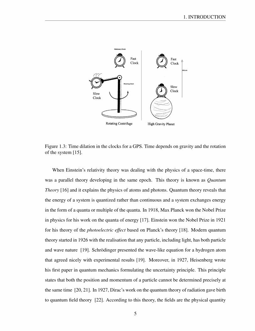
In our daily life, the most useful application of the relativistic theory is the GPS [9].
GPS provides the location and time of a GPS receiver on or near the Earth and hence
this system is very effective for airlines, military, even in our everyday technology like
smart phones, cars, etc. The GPS satellites revolve around the earth in outer space and they
contain clocks that are needed to be synchronized properly in order to get an accurate signal.
GPS technology uses both special and general theory of relativity in order to improve the
system’s accuracy. According to the special theory of relativity, clocks on the satellites
should be 7 microseconds/day slower due to their motion [9]. On the other hand, according
to the general theory of relativity, clocks on the ground should be 45 microseconds/day
slower because of the effective curvature of the space-time near the Earth [9]. In Figure
1.3, the left part is showing the effect due to special theory of relativity where the rotating
clocks are slower than the stationary clocks. The right part of Figure 1.3 is showing the
effect of general theory of relativity where the clock, sitting on the Earth, is slower than the
clock sitting on higher altitude. Altogether, there should be 38 microseconds/day correction
in the GPS. There are also other ideas, like time travel [13], worm holes [14]. that originate
from the general theory of relativity.
4
1. INTRODUCTION
Figure 1.3: Time dilation in the clocks for a GPS. Time depends on gravity and the rotationof the system [15].
When Einstein’s relativity theory was dealing with the physics of a space-time, there
was a parallel theory developing in the same epoch. This theory is known as Quantum
Theory [16] and it explains the physics of atoms and photons. Quantum theory reveals that
the energy of a system is quantized rather than continuous and a system exchanges energy
in the form of a quanta or multiple of the quanta. In 1918, Max Planck won the Nobel Prize
in physics for his work on the quanta of energy [17]. Einstein won the Nobel Prize in 1921
for his theory of the photoelectric effect based on Planck’s theory [18]. Modern quantum
theory started in 1926 with the realisation that any particle, including light, has both particle
and wave nature [19]. Schrodinger presented the wave-like equation for a hydrogen atom
that agreed nicely with experimental results [19]. Moreover, in 1927, Heisenberg wrote
his first paper in quantum mechanics formulating the uncertainty principle. This principle
states that both the position and momentum of a particle cannot be determined precisely at
the same time [20, 21]. In 1927, Dirac’s work on the quantum theory of radiation gave birth
to quantum field theory [22]. According to this theory, the fields are the physical quantity
5

1.1. THIS THESIS
and particles are the excited state of the field. Quantum theory is quite well-developed now
and this theory has been rigorously verified in experiments [23].
Quantum mechanics and quantum field theory, both have a huge application in different
fields of technology including supercomputers, semiconductors, superconductors, particle
accelerators, ultra-precise clocks [24, 25, 26, 27]. Quantum mechanics is needed in bio-
physics, condensed matter and quantum chemistry [28]. Three of the four fundamental
interactions of the universe, viz. electromagnetic interaction, strong and weak interac-
tions, have been quantized using quantum field theory and experimentally well-verified
[29]. However, quantisation of the gravitational interaction is still not mathematically well-
formulated [30].
Understanding physics behind how the universe works, becomes even more challeng-
ing when one introduces quantum theory in general relativity. Starting from 1930 to the
present, the quantum theory of gravity has come a long way through different formalisms
and methodologies [31]. However, it is still a developing area of physics with many unan-
swered questions. For now, we do not have any experimental evidence of quantum gravity
because of the inability of constructing a proper instrumental set up to study the weak effect
at the quantum length scale (Planck length scale ∼ O(10−35m)) [32]. Therefore, none of
the quantum gravity theory has been verified yet. Although there are a number of candidate
models trying to quantize gravity theoretically, String theory and Loop quantum gravity are
the most promising theories among the models [33]. Throughout this thesis, we will follow
the loop quantum gravity approach. It is to be noted that there is no consistent theoretical
model to explain all the features of the quantum gravity. Hence, it is expected we will
have some ‘yet to be answered’ questions at the very end of this thesis. Research is still
continuing and hopefully we will able to answer all the queries in the very near future.
6

1.1. THIS THESIS
1.1 This Thesis
There is no straight forward method to quantize gravity theoretically and observe the
gravity quanta “graviton” experimentally. The theories “General relativity” and “relativistic
quantum mechanics” both of the theories work great on their own. However, the combina-
tion of these two theories does not lead us to a fruitful solution, rather ends up with infinite
number of divergences. Therefore, theorists have been trying to quantize gravity in differ-
ent approaches in order to avoid the divergences [31]. Many of these theoretical approaches
are quite successful in providing a quantum description of the space-time even though none
of them are experimentally verified, hence unreliable. Experimentally detectable evidence
for the quantum nature of gravity is still not achieved by the modern technology. One of the
main reasons is the weakness of the gravitational interaction. In order to get a detectable
quantum gravity effect at Planck length scale, we need to produce extremely high energy
(≈ 1030 eV ) where the latest generation can only produce 1013 eV [34]. However, given
a classical space-time, quantum fluctuations, though infinitesimal, might affect phenomena
which are observable. This is not unusual in quantum physics as tiny quantum fluctuations
produce the Casimir effect detectable in ‘classical’ quantum plates [35]. The main purpose
of this thesis is to find an observable effect due to a semi-classical correction found in loop
quantum gravity coherent states.
A quantum effect can be implemented as a semi-classical correction in the classical
space-time. Even though the correction is too small to detect directly, it might generate
a non-trivial effect in the space-time due to the non-linearity of the mathematical equa-
tions describing the system. The semi-classical correction has been computed for the
Schwarzschild black hole space-time which is a solution of the Einstein’s equations. The
computed correction has broken the spherical symmetry of the Schwarzschild black hole.
Due to the non-linearity of the Einstein’s equations, the correction effect might take a
chaotic form near the unstable orbits of the Schwarzschild black hole under certain con-
7

1.1. THIS THESIS
ditions [36]. In this thesis, we have observed different field propagation in this corrected
black hole background. The correction will distort this background space-time and hence
effects of the distortion can be calculated on the field propagation. We have studied the cor-
rection effect in the scalar and vector propagation near the black hole event horizon where
this quantum effect is maximum. For the tensor propagation, we have the equations which
are to be solved numerically. As a result, we have found non-trivial loop quantum gravity
correction effects in each of the fields.
• For the scalar field propagation, the semi-classical correction is introducing a left-
right asymmetry in the propagation of a Gaussian wave near the black hole horizon.
We have studied the effect using a toy model wave-equation and solved the equation
numerically with proper boundary conditions. We have shown the correction effect
is not only breaking the symmetry of the solution, but the velocity of propagation
also depends on the correction. The scalar field equation with the actual quantum
gravitational correction term also shows assymmetry as the toy model, we have taken.
However, this work is still in progress and will be presented soon. The outcome of
this research might have some consequences for Hawking radiation [37], which can
be observed experimentally [38].
• For the vector field propagation in the corrected black hole background, the semi-
classical correction is generating a radial component of the vector potential which is
missing in the classical solution. The angular component of the vector potential will
also have correction. As the black hole entropy depends on the vector potential, our
result might have a non-trivial effect on the entropy of the system. In the upcoming
years, we are also expecting to have an event horizon telescope that would be able
to observe the high gravity zone [39]. As telescope technology is based on the light
wave propagation, i.e. vector field propagation, the correction effect might give a
relevant prediction of observation.
8
1.2. OUTLINE
• For the tensor field propagation, i.e. the gravitational wave propagation, we have
found non-trivial equations that might be analysed numerically. The equations, we
found, are quite complicated to solve as there is no symmetry in the system, and the
solutions will be in most general form. In particular, there is no ‘odd’ and ‘even’
parity modes of the spherical gravitational wave. However, this complexity might
bring good news as we are looking for a chaotic effect in the system. A gravity wave
has already been detected [7] at the end of 2015. Therefore, we can expect better
technology that might be able to detect this quantum correction effect in the near
future.
1.2 Outline
We will start this thesis with a brief demonstration of the background theories: Ein-
stein’s special theory of relativity and general theory of relativity, in Chapter 2. In this
chapter, it will be shown that the curvature of the space-time due to the presence of the mat-
ter and energy can be depicted as the cause of gravitational force. This phenomenon can be
represented by Einstein’s field equations. The simplest vacuum solution of these equations,
characterizing an uncharged non-rotating black hole space-time, namely Schwarzschild
black hole, will also be derived.
In Chapter 3, quantum theory of gravity will be introduced. The quantum gravity theory
is a big field of research by itself and consists of different ideas of quantization. For our
purpose, mainly the basic theories relevant to this thesis will be discussed and we will use
the results directly in later calculations.
The original work of this thesis will begin in Chapter 4. In this chapter, a correction will
be calculated from loop quantum gravity coherent state in Schwarzschild black hole back-
ground and we will observe this quantum effect of gravity on the scalar field propagation
in the Schwarzschild black hole background. The result of this research will be calculated
numerically.
9

1.3. NOTATION
Next in Chapter 5, quantum gravity effect will be discussed on the vector field propaga-
tion with the black hole background. We will analyse the outcome of the correction effect
on the vector field.
Finally, we conclude in the last chapter and summarize the findings based on what
we are looking for and what we have found. We also discuss quantum gravity effect on
the tensor field propagation which is a work in progress. Some new research possibilities
related to this thesis will also be recommended in this chapter.
1.3 Notations and Representation
1.3.1 General Notations
• In this thesis, we will deal with the three and four dimensional coordinate systems.
The three dimensional space coordinates x, y, z will be expressed as xi or xi where
the index i = 1,2,3 respectively. The index i will be replaced often by j or k or
other Latin letters. Hence coordinates with Latin indices will represent the three
dimensional space. On the other hand, four dimensional space-time coordinates t, x,
y, z will be expressed as xµ or xµ where the index µ = 0,1,2,3 respectively. Again,
the index µ can be replaced by ν, τ or any Greek letters. Therefore, the coordinates
with Greek indices will represent the four dimensional space-time. Accordingly, the
partial derivative operators ∂i and ∂µ denote the partial derivative operation ∂
∂x for
i, µ = 1.
• We have used Einstein summation convention in the entire thesis. There will be
summation over any repeated index. For example in three dimensions, xixi = x1x1 +
x2x2 + x3x3 [40].
• The ‘Prime’ sign over a mathematical variable denotes the derivative with respect
to space coordinates unless it is stated otherwise. Example: For an arbitrary factor
A, A′ ≡ dAdx . The ‘dot’ sign over a mathematical variable implies the derivative with
10

1.3. NOTATION
respect to time coordinate. Example: For a factor A, A≡ dAdt .
• Bold mathematical characters are denoted as the vector quantities. For example, for
a vector quantity B, B≡ ~B.
1.3.2 Coordinate System
In this section we will discuss the coordinate system briefly [41]. A coordinate system
uniquely defines the position of a point in space. Cartesian coordinate system is one of the
simplest systems in geometry.
In three dimension, the Cartesian coordinate system is made of three perpendicular axes X,
Y, Z and the intersection of the three axes is known as the origin.
Figure 1.4: Cartesian coordinate system
The position of a point P is given by a set of
three unique numbers (x,y,z) where x, y, z are
the distances of the point from the origin along
the X, Y, Z axes respectively as shown in Figure
1.4. The infinitesimal path difference between
two points in this coordinate system is given by
ds2 = dx2 +dy2 +dz2.
Figure 1.5: Spherical coordinate system
Spherical coordinate system is another
way to define the position of a point in
space. In Figure 1.5, the position of the
point P has been defined with three unique
numbers (r,θ,φ) where r is the radial dis-
tance from the origin to the point P, θ is the
polar angle between the Z axis and the ra-
dial distance, φ is the azimuthal angle be-
tween the X axis and the radial projection
on the X-Y plane. The infinitesimal path difference between two points in this coordinate
11
1.3. NOTATION
system is given by ds2 = dr2 + r2dθ2 + r2 sin2θ dφ2.
Later in this thesis, we will introduce time t as a coordinate. In order to determine
the location of a point in four dimensional space-time, we would need a time axis along
with three space axes. This time axis is perpendicular to each of the space axes. However,
in mathematical calculations, it would be considered that the time axis is imaginary. The
infinitesimal path difference between two points in four dimensional space-time is given
by, ds2 = −dt2 + dx2 + dy2 + dz2 or ds2 = −dt2 + dr2 + r2dθ2 + r2 sin2θ dφ2. We have
used natural units here with c = 1. Sometimes, in this thesis, we will use natural units with
c = ~= G = 1 for convenience [42]. It is to be noted there is a−ve sign associated with the
time coordinate, i.e, the four dimensional path difference is following the sign convention
(- + + +) [43]. We will be using this convention through out this thesis. One can always
alter the sign convention to (+ - - -) with a +ve time and −ve space components, but the
physics of the system will still be the same. However, in order to avoid the confusion, a
particular sign convention should be followed entirely in a mathematical calculation.
12

Chapter 2
Classical Gravity
Black holes are where
God divided by zero.
– A. Einstein
The central idea of this chapter is to show that gravity arises due to the curvature of the
geometry of a four dimensional space-time. According to the principle of least action, a
moving particle should always choose the path that will extremize the action of the system
[44]. Typically, for Newtonian mechanics the chosen path is the shortest possible straight
line between the starting and ending positions. For example, if you leave a ball at the higher
side of an inclined plane, the ball will slide along a straight line on the plane. Now the
question is, what will be the trajectory of the ball if the inclined plane is a curved surface.
Obviously, the ball will follow the curved surface. So, the geometry of the space has an
important role in the movement of the particle. This example is just an over-simplified
model of the actual scenario for the curvature in the space-time. However, the point is, if a
space-time is significantly curved, even the trajectory of light can bend [45].
This chapter is a review chapter based on Einstein’s theory of special and general theory
of relativity. We will start this chapter with the idea of flat space-time described by special
theory of relativity. In the following section, we will discuss the required differential geom-
etry in order to compute the mathematical model for the curved space-time. We will also
discuss Einstein’s field equations that describe any geometry in curved space-time. Finally
13

2.1. SPECIAL THEORY OF RELATIVITY
the simplest solution of Einstein’s field equations, namely Schwarzschild solution, will be
presented. In this work, the background space-time is taken to be Schwarzschild black hole
space-time. Therefore, a brief discussion on the nature of this space-time would be relevant
in this context.
2.1 Special Theory of Relativity
Special theory of relativity is an experimentally well-verified theory developed by Ein-
stein in 1905 [46]. This theory has introduced modification to Newtonian mechanics for
systems with high velocity comparable to the velocity of light. The original Newtonian
mechanics can describe the physics only when the dimension of the system is somewhere
between micron length and cosmological length, the reference frame is inertial, i.e. the
frame is not accelerating with respect to obeserver’s reference frame, does not have many
degrees of freedom, in addition, the particles within the system does not approach the ve-
locity of light. Special theory of relativity introduces modifications to macroscopic high
velocity system with small degrees of freedom. This theory is based on two postulates pro-
posed by Einstein [1],
Principle 1: The laws of physics are the same in any inertial frame, regardless of posi-
tion or velocity.
Principle 2: The speed of light in free space is constant (generally defined as c) in all
inertial frame of reference.
Special theory of relativity considers time on the same footing as space. Hence, instead
of using the three dimensions of space and one absolute time, a unified four dimensional
space-time coordinate system is defined. An individual point in the four dimensional space-
time is called a world-point compared to position in three dimensional space [46, 47, 48].
14

2.1. SPECIAL THEORY OF RELATIVITY
The geometry of any space-time can be described by the line element: the infinitesimal
path difference between two world-points in the space-time. In three dimensional Cartesian
coordinate, the line element ds describing a Euclidean geometry is given by the metric ds2
as,
ds2 = dx2 +dy2 +dz2 . (2.1)
However, in four dimensional space-time geometry, the line element in natural unit c = 1 is
described as,
ds2 = −dt2 +dx2 +dy2 +dz2
⇒ ds2 = ηµνdxµdxν , (2.2)
where µ,ν runs from 0 to 3. The geometry defined by equations (2.2) is different from the
Euclidean geometry because of the−ve sign presented in the metric. This geometry is often
called Minkowski space or flat space-time [1]. The second equation in the equations (2.2)
is a tensor form of the metric where ηµν is known as Minkowski metric tensor given by a
4×4 matrix,
ηµν =
−1 0 0 0
0 1 0 0
0 0 1 0
0 0 0 1
. (2.3)
Also, it is important to note that the quantity ds2 is invariant in all inertial frames of
reference and ηµν is a symmetric tensor. Inverse metric of ηµν is given by ηµν such that
ηµνηµτ = δτν [1].
Depending on the positivity or negativity of ds2, one can portray different scenario in the
15
2.1. SPECIAL THEORY OF RELATIVITY
four dimensional space-time. Considering a particle movement just in x direction, two
points in the space-time is separated by the distance, ds2 =−dt2 +dx2.
(i) When ds2 > 0: The pair of world-points is said to be space-like separated, e.g., dt = 0,
dx 6= 0 or dt < dx. It implies that two points can be space-like separated but no
information can be exchanged between them as it violates the causality.
(ii) When ds2 < 0: The pair of world-points is said to be time-like separated, e.g., dt 6= 0,
dx = 0 or dt > dx. It implies that two points which are time-like separated can exchange
information as one is in the causal past of the other.
(iii) When ds2 = 0: The pair of world-points is said to be light-like/null separated, e.g.,
dx = dt. In this case, points are connected with light rays. One can say this is the
boundary of the time-like and space-like region.
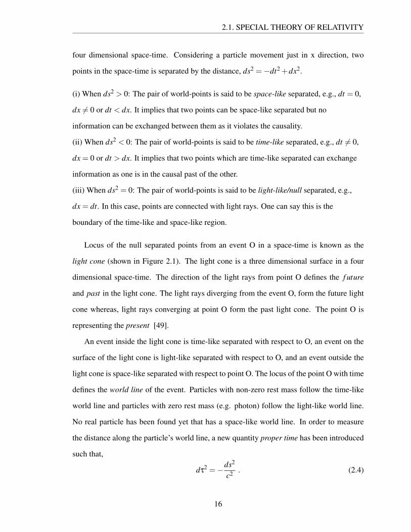
Locus of the null separated points from an event O in a space-time is known as the
light cone (shown in Figure 2.1). The light cone is a three dimensional surface in a four
dimensional space-time. The direction of the light rays from point O defines the f uture
and past in the light cone. The light rays diverging from the event O, form the future light
cone whereas, light rays converging at point O form the past light cone. The point O is
representing the present [49].
An event inside the light cone is time-like separated with respect to O, an event on the
surface of the light cone is light-like separated with respect to O, and an event outside the
light cone is space-like separated with respect to point O. The locus of the point O with time
defines the world line of the event. Particles with non-zero rest mass follow the time-like
world line and particles with zero rest mass (e.g. photon) follow the light-like world line.
No real particle has been found yet that has a space-like world line. In order to measure
the distance along the particle’s world line, a new quantity proper time has been introduced
such that,
dτ2 =−ds2
c2 . (2.4)
16

2.1. SPECIAL THEORY OF RELATIVITY
Figure 2.1: Light cone for a event O. Space-like, time-like and light-like separated pointswith respect to O are shown with points E1,E2,E3 [50].
This is the time measured by the inertial frame along its own world line. This is the way
Einstein introduced time as a coordinate in the geometry of a system [51].
A new transformation law for this relativistic theory was proposed by Einstein instead
of Galilean transformation used in Newtonian mechanics [46]. According to the princi-
ple of the Special Theory of Relativity, as ds2 is invariant in different inertial frames, the
transformation from the coordinates (t,x,y,z) to (t ′,x′,y′,z′) should preserve the form of
the equation (2.2). This transformation is known as Lorentz transformation [52] ( It is
to be noted that the ‘prime’ sign over (t,x,y,z) is denoting the transformed coordinates, it
is not representing the derivative of space). If we consider one inertial frame is moving
with a constant velocity v along x axis with respect to the other inertial frame, the Lorentz
17

2.1. SPECIAL THEORY OF RELATIVITY
transformation between two frames are given by,
t ′ = γ(t− vx/c2)
x′ = γ(x− vt)
y′ = y
z′ = z , (2.5)
with γ = 1√1−v2/c2
. However, the inverse transformation is given by,
t = γ(t ′+ vx′/c2)
x = γ(x′+ vt ′)
y = y′
z = z′ . (2.6)
In the tensor form, the Lorentz transformation can be written as,
x′ν = Λνµxµ , (2.7)
where Λνµ is the Lorentz transformation metric. For the boost along the x direction with
velocity v, the metric takes the form,
Λνµ =
γ −βγ 0 0
−βγ γ 0 0
0 0 1 0
0 0 0 1
, (2.8)
where β = vc .
The special theory of relativity gives us a few consequences that are experimentally
18

2.1. SPECIAL THEORY OF RELATIVITY
verified [53, 54]. One of the important consequence is the relativity of simultaneity. Time
interval ∆t also transforms as the first equation of the equations (2.5). If ∆t = 0, i.e., two
events are occurring at the same time in different locations (∆x 6= 0) observed from one in-
ertial reference frame, then we find ∆t ′ 6= 0, i.e., the events are not simultaneous as observed
from another inertial frame of reference. The same equation also yields the time dilation
property for an event. If an event is observed from an inertial frame of reference for a time
period ∆t, the same event in the same location (∆x = 0) will appear to take a longer time
period, ∆t ′= γ∆t as observed from another inertial reference frame. The second equation of
the equations (2.6) gives us the paradox of length contraction. Suppose the length of a rod
measured in its inertial reference rest frame is ∆x. If the length is measured simultaneously
from another reference frame, the length will appear contracted as ∆x′ = ∆xγ
.
Now let us consider a particle moving with a velocity u′ along x axis in a reference
frame S′. If S′ is moving with the velocity v along x axis with respect to another inertial
reference frame S, then the velocity of the particle observed by S,
u =dxdt
=u′+ v
1+ u′vc2
. (2.9)
It is to be noted that with the limit u′,v c, the velocity will follow the Galilean trans-
formation rule u = u′+ v. Also, for u′ = c, one can find from equation (2.9) that u = c.
Hence this theory states that the velocity of light is independent of the frame of reference.
Special theory of relativity has achieved huge success for the relativistic systems, spe-
cially in the astrophysics and cosmology [55]. Maxwell’s equations are found to be special
relativistic theory invariant but not Newtonian gravity. Though Newtonian gravity could
explain most of the planetary motion of our solar system, it could not justify the perihe-
lion precession of the Mercury. In 1915, Einstein published his article on General Theory
of Relativity where gravity was visualized in a completely unique way [56]. In general
theory of relativity, gravity is defined as a consequence of curvature in four dimensional
19

2.2. RIEMANNIAN GEOMETRY AND EINSTEIN’S FIELD EQUATION
space-time rather than an attractive force between two objects as defined in Newtonian the-
ory. The curvature in space-time is caused by the presence of matter or energy. This new
theory not only explains the perihelion precession of Mercury [4], but also reveals some
other astrophysical phenomena including bending of light rays, gravitational time dilation,
existence of gravity wave and black holes [56, 1].
2.2 Riemannian Geometry and Einstein’s Field Equation
Manifold and Differential Manifold:
Einstein’s general theory of relativity is a generalization of the special theory of relativity
where the Minkowskian flat space-time is replaced by a curved space-time. In order to
study the physics in the curved space-time, first we need to build the basic formalism to de-
scribe the curved space-time. In this section, we will study the basic mathematics to obtain
the curvature of a given geometry. We will be using Riemannian Geometry for this purpose
[57]. We will begin our study with the understanding of the Manifold.
Definition 2.1. A manifold is defined as an n-dimensional space (any kind of topological
space) which is locally equivalent to n-dimensional Euclidean space Rn. An n-dimensional
manifold will have open sets homeomorphic to Euclidean geometry. If time is included,
then the manifold is locally equivalent to Minkowski space-time [57].
For example, an n-dimensional sphere Sn is a manifold where a circle is S1 sphere, a
2-sphere is S2 etc. It is obvious that an n-dimensional Euclidean space Rn is also a manifold
as it is locally Euclidean. There are some geometries that cannot be regarded as a manifold,
e.g., a one dimensional line intersecting a two dimensional plane. Here the intersection
point cannot be mapped into a Euclidean space. In order to study a concrete example, let
us define a map. Map ξ is defined as a relationship between two sets M and N such that
ξ : M→ N, i.e., for each element of M, there is one element for N. For the S1 circle with
20

2.2. RIEMANNIAN GEOMETRY AND EINSTEIN’S FIELD EQUATION
unit radius, we can write the circle as an union of open sets, each of which maps to R [58],
ξ1 := (x,y)|x > 0 φ1(x,y) := y
ξ2 := (x,y)|x < 0 φ2(x,y) := y
ξ3 := (x,y)|y > 0 φ3(x,y) := x
ξ4 := (x,y)|y < 0 φ4(x,y) := x , (2.10)
where the constraint equation is x2+y2 = 1. Thus the circle is mapped into a real Euclidean
line. It is to be noted that even though the circle is written as a function of both x and y, the
constraint equation reduces one degree of freedom making it one dimensional geometry.
Note: There is also an inverse mapping that exists such that ξ−1 : N →M and for an ele-
ment a of set M, ξ.ξ−1(a) = a.
In general relativity, the 4-dimensional space-time is a special class of manifold which
is differentiable and is known as a differential manifold. Let us consider a map ξ : Rm(x)→
Rn(y), such that,
y1 = ξ1(x1,x2, ...,xm)
y2 = ξ2(x1,x2, ...,xm)
...
yn = ξn(x1,x2, ...,xm) . (2.11)
Any of these functions can be referred to as a Cp map where the function is continuous
and p times differentiable. A smooth manifold should have a C∞ mapping.
Tangent Space, Vector and Dual Vector:
Now let us define a tangent space on a differential manifold. First we consider a manifold
21

2.2. RIEMANNIAN GEOMETRY AND EINSTEIN’S FIELD EQUATION
M with smooth functions such that a C∞ map f : M→ R exists and we draw curves on this
space through an arbitrary point p. Now we can define an operator in that space, named
directional derivative, which maps f → d fdλ
at p where λ is a parameter along the curve.
Definition 2.2. A tangent space τp is defined as a space of the directional derivative opera-
tors along the curves through the point p [59].
The directional derivative operator is actually representing a vector which can be de-
fined as an arrow in the space-time with a notion of direction. It is often convenient to
decompose a vector into components along a set of basis vectors, where the basis vectors
are independent of each other. Any abstract vector A can be written as a linear combination
of basis vectors eµ and its components Aµ,
A = Aµeµ , (2.12)
where the index µ is assigned to the numbers of dimension of the space and takes the values
0,1,2,3... accordingly. Sometimes, in physics, we loosely refer a vector A as its components
Aµ when the basis vectors are known. On a differential manifold at each point x, we can find
a tangent space where we can define vectors V = V µ ∂
∂xµ = V µ∂µ ( ∂µ represents the basis
on the tangent space and V µ are the components). The way V µ transform under change of
coordinates gives them the label contravariant vectors. Under a coordinate transformation
µ→ µ′, the contravariant vector component changes as,
V µ′ =∂xµ′
∂xµ V µ . (2.13)
We can also define dual vectors corresponding to the vectors such that the dual vectors
map vectors to real numbers. There is an easy way to visualize the difference between a
vector and a dual vector as shown in reference [59]. If we visualize a vector as an arrow,
then a dual vector can be visualized as a series of parallel surfaces. When the arrow ‘vector’
passes through the parallel surfaces ‘dual-vector’ the vector is said to be mapped by the dual
22

2.2. RIEMANNIAN GEOMETRY AND EINSTEIN’S FIELD EQUATION
vector. The dual vector maps the vector into real number which can be visualized as the
number of surfaces the arrow pierces. Mathematically, the dual vector ω is expressed as,
ω = ωµeµ , (2.14)
where eµ are the basis dual vectors and ωµ are the components. Therefore, we can also
define a dual space to the tangent space known as the cotangent space such that the dual
vectors ω = ωµdxµ maps the tangent vectors to the space of real numbers (dxµ are the
basis of the cotangent space and ωµ are the components). The way, the ωµ transform un-
der coordinate transformation, gives them the label covariant vectors. Under a coordinate
transformation µ→ µ′, the covariant vector components change as,
ωµ′ =∂xµ
∂xµ′ωµ . (2.15)
Note: It is to be noted that contravariant vector components are referred to with upper in-
dices and the basis vectors are referred to with lower indices. For the covariant vector, the
components are referred to with lower indices and the basis vectors are referred to with
upper indices.
Tensors:
A generalization of vectors and dual vectors leads us to define another quantity named
tensor. We can define tensor T that transforms in both of the tangent and cotangent space,
e.g. T = T i jlmk∂i⊗∂ j⊗dxl⊗dxm⊗dxk, where T is a T (2,3) type tensor. A tensor of (m,n)
type should have m number of contravariant indices and n number of covariant indices.
Therefore, from this point of view, a scalar is a (0,0) type tensor, a vector is a (1,0) type
tensor and a dual vector is a (0,1) type tensor. It can be said that while a dual vector maps
a vector to a real number, a tensor is a multilinear map from a collection of vectors and
dual vectors to real numbers. An N dimensional two tensor ((2,0),(0,2) or (1,1) type) can
23
2.2. RIEMANNIAN GEOMETRY AND EINSTEIN’S FIELD EQUATION
be written as an N×N matrix. On our four dimensional manifold, all the tensors are 4×4
matrices. For example, in the special theory of relativity, the Minkowski metric tensor ηµν
can be written as a 4×4 matrix as shown in equation (2.3) and it is a tensor of type (0,2).
One of the characteristics of the differential manifold is the concept of the distance
function. As we have already seen in equation (2.3), the line element in the space-time
can be represented in terms of ηµν which is the diagonal metric tensor of the Minkowski
space-time. The generalization of this tensor to arbitrary curved geometries is gµν which
is a symmetric metric tensor. With this metric, the notion of distance is ds2 = gµνdxµdxν.
In this way, the metric of space-time is used to map a contravariant tensor to a covariant
tensor.
Vµ = gµνV ν . (2.16)
A metric tensor contains all the information that we need to describe the curvature of the
manifold and it has a non-vanishing determinant g = |gµν|. As gµν is symmetric in µ and
ν, it has 10 independent components. The inverse metric tensor gµν can also be defined
as gµνgµλ = δν
λ. Later in this chapter, we will derive the metric tensor components for the
Schwarzschild black hole space-time.
Another important tensor in general relativity is the Stress-energy tensor T µν [57]. This
is a type (2,0) symmetric tensor which provides the information of the energy, momenta,
pressure, etc. of the system. The quantity T µν stands for flux of four-momentum pµ across
a surface of constant xβ [59]. Thus the components T 00 refers to the energy density,
T 0i = T i0 refers to the energy flux or momentum density, and T i j refers to the momentum
flux or stress of the system. In general relativity, any matter or field can be described as a
perfect fluid which is ‘isotropic in its rest frame’ [12]. For a perfect fluid with density ρ
and pressure p, the stress-energy tensor is given by,
T µν = (ρ+ p)uµuν + pηµν , (2.17)
24

2.2. RIEMANNIAN GEOMETRY AND EINSTEIN’S FIELD EQUATION
where uµ is the four-velocity of the system.
Derivative, Parallel Transport and Geodesic:
Now we will see how vectors and tensors behave with change of space-time point. When
a vector or tensor moves on the manifold, we need to introduce a connection which is
characterized by the curvature of the manifold. In flat space-time, change of any vector
or tensor can be mapped by the partial derivative operator where no connection is needed.
In flat space-time, the derivative of a vector V ν in the direction xµ is given by ∂µV ν and
it is sufficient to describe the whole scenario. However in curved geometries, the vector
components also get rotated. To measure this rotation, we introduce an affine connection
[59] (also called Christoffel symbols) Γλµν on the differential manifold. The total derivative,
symbolically ∇µ, is defined as the regular partial derivative and the connection. This total
derivative is known as the covariant derivative.
Definition 2.3. A derivative operator on a manifold M , which takes a tensor field of type
T (k, l) to type T (k, l +1) is known as a covariant derivative [57].
For the covariant vector Vν, the covariant derivative is given by,
∇µVν = ∂µVν−ΓαµνVα . (2.18)
For the contravariant vector V ν, the covariant derivative is given by,
∇µV ν = ∂µV ν +ΓνµαV α . (2.19)
The affine connection is not a tensor because under a coordinate transformation, it does not
transform like a tensor. Also it is symmetric in the lower two indices. This property will be
shown later when we obtain an expression for this connection. In general, for an arbitrary
25

2.2. RIEMANNIAN GEOMETRY AND EINSTEIN’S FIELD EQUATION
Figure 2.2: Parallel transport of a vector on the surface of a two sphere. The vector isrotated at the ending point after following a different path [60].
tensor, one can write,
∇σV µ1µ2µ3...µkν1ν2ν3...νk = ∂σV µ1µ2µ3...µk
ν1ν2ν3...νk +Γµ1σλ
V λµ2µ3...µkν1ν2ν3...νk +Γ
µ2σλ
V µ1λµ3...µkν1ν2ν3...νk + ...
−Γλσν1
V µ1µ2µ3...µkλν2ν3...νk
−Γλσν2
V µ1µ2µ3...µkν1λν3...νk
− ... . (2.20)
Now we have the mathematical tools to find the derivative of a vector or tensor in a
curved manifold. Here, we will discuss the notion of parallel transport.
Definition 2.4. If a vector remains parallel to itself when transported along a curve, then it
is said to be parallel transported [59].
In flat space-time, the parallel transport of a vector does not depend on the path. How-
ever, in curved space-time, the choice of path is important while parallel transporting a
vector. In the Figure 2.2, it has been shown that, the vector might not return to the same
point to be coincident with itself. This is the sign of existence of curvature in the manifold.
A vector is said to be parallel transported along a path if tµ∇µV ν = 0, where tµ represents
the tangent vector to the curve.
With the understanding of parallel transport, the next logical discussion is about the
Geodesic. We know in flat space-time a force-free particle moves in a straight line which
is the shortest distance possible between two points. However, in curved space-time, the
curve that connects the shortest distance between two points, is called the geodesic. In
terms of parallel transport, one can say,
26

2.2. RIEMANNIAN GEOMETRY AND EINSTEIN’S FIELD EQUATION
Definition 2.5. A geodesic is a curve which parallel transports its own tangent vector [59].
A force-free particle follows a geodesic in the curved space-time. The equation of
motion of a test particle in a particular space-time can be derived by taking the variation
on the metric. According to the variational principle, the world line between two time-like
separated points of a test particle would extremize the proper time. This statement leads us
to write,
δ
∫ds = 0 . (2.21)
For the flat space-time, the line element is ds =√−ηµνdxµdxν and hence the equation of
motion can be expressed as,d2xµ
dτ2 = 0 . (2.22)
On the other hand, for the curved space-time with ds =√−gµνdxµdxν, the equation of
motion can be written as,d2xµ
dτ2 +Γµαβ
dxα
dτ
dxβ
dτ= 0 (2.23)
⇒ uν∇νuµ = 0 , (2.24)
where uν is the four-velocity of the particle. The above equation is a set of four equations
with the free index µ = 0,1,2,3. These equations of motion of a particle in a curved space-
time are known as geodesic equations [57]. It is to be noted that the geodesic equations are
free particle equations without any force. If a particle moves under some forces, then the
force terms can be added on the LHS of the equation (2.23). For the time-like geodesic,
we consider proper time τ as the parameter along the geodesic. However, for the light-like
geodesic, time is not defined any more; hence we introduce some affine parameter that
characterizes the geodesic [59].
Curvature and Gravity:
Curvature of a space-time can be quantified by a quantity called Riemann Curvature. We al-
27

2.2. RIEMANNIAN GEOMETRY AND EINSTEIN’S FIELD EQUATION
ready know the fact that a vector changes while parallel transported along different paths on
the manifold. The change of the vector carries the information of the curvature.
P
Q
Ι
ΙΙ
ΙΙΙ
IV
Figure 2.3: Commutator of covari-ant derivatives [61].
In order to quantify the curvature, we refer to Fig-
ure (2.3). In this figure we parallel transport a vector
from P to Q along two different paths. Path 1 is fol-
lowing path I and II, and path 2 is following path III
and IV as labelled in the figure. The change along
path 1 is found as ∇µ∇νV ρ (We assume that the tan-
gent vectors to path I and II are constants). Similarly
the change along path 2 is ∇ν∇µV ρ. Next we take
the difference of the two paths, and find that,
∇µ∇νV ρ−∇ν∇µV ρ = [∇µ,∇ν]V ρ
= (∂µΓρ
νσ−∂νΓρ
µσ +Γρ
µλΓ
λµσ−Γ
ρ
νλΓ
λµσ)V
σ
−Γρ
µσΓσ
νλV λ−Γ
ρ
νσΓσ
µλV λ , (2.25)
where [∇µ,∇ν] is the standard commutator bracket in mechanics. The first bracketed part in
the equation (2.25) is known as the Riemann Curvature of the manifold and given by [59],
Rρ
σµν = ∂µΓρ
νσ−∂νΓρ
µσ +Γρ
µλΓ
λµσ−Γ
ρ
νλΓ
λµσ . (2.26)
A nonzero Riemann tensor signifies the existence of curvature. The other quantity in equa-
tion (2.25) measures torsion, and is zero for space-times which are ‘metric’ compatible, i.e.,
the parallel transport of a metric along any path is zero.
∇λgµν = 0 . (2.27)
The above equation can be solved to give a formula for the affine connection, which is
28

2.2. RIEMANNIAN GEOMETRY AND EINSTEIN’S FIELD EQUATION
symmetric in the lower indices.
Γλµν =
12
gλρ(∂νgµρ +∂µgλν−∂λgµν
). (2.28)
There are few symmetries associated with the Riemann tensor and it is easy to see if we
lower all of the indices using the relation Rρσµν = gρλRλσµν. The symmetries in the tensor
Rρσµν can be described as follows:
• Antisymmetric in the first two indices such that, Rρσµν =−Rσρµν.
• Symmetric in the first two pair of indices to the second two pair of indices such that,
Rρσµν = Rµνρσ.
• Follower of the relation Rρσµν +Rρνσµ +Rρµνσ = 0.
After applying these constraints it is easy to calculate the number of the independent com-
ponents of the Riemann tensor. For the four dimensional space-time, it has 20 independent
components. Along with the above mentioned symmetries, there is a differential identity
for the Riemann tensor,
∇λRρσµν +∇ρRσλµν +∇σRλρµν = 0 . (2.29)
The above identity is known as Bianchi identity [43].
Sometimes it is possible to use a contracted form of the Riemann tensor. This contracted
form is known as the Ricci tensor and it is given by [59],
Rµν = Rαµαν
= ∂αΓαµν−∂νΓ
αµα +Γ
ασαΓ
σνµ−Γ
ασνΓ
σαµ . (2.30)
It is to be noted that the Ricci tensor is symmetric as Rµν = Rνµ. With further contraction,
29

2.2. RIEMANNIAN GEOMETRY AND EINSTEIN’S FIELD EQUATION
one will end up with the Ricci scalar [59],
R = gµνRµν = Rµµ
= gµν(∂αΓαµν−∂νΓ
αµα +Γ
ασαΓ
σνµ−Γ
ασνΓ
σαµ) . (2.31)
If we contract the identity equation (2.29) with gµσgνλ, we will get the following,
∇µRρµ =
12
∇ρR . (2.32)
This equation can be re-written as,
∇µGµν = 0 , (2.33)
where Gµν is known as the Einstein tensor and it is defined as [59],
Gµν = Rµν−12
Rgµν . (2.34)
Now we have a formalism for a curved manifold described by the Riemann tensor, Ricci
tensor and Ricci scalar. The curvature, we have computed here, is referred as ‘intrinsic
curvature’. This curvature can be measured by the observer who is staying on the same
dimension as the manifold. For our four dimensional manifold, the intrinsic curvature is
measured by the observers who are on the four dimensional manifold by themselves. There
is also ‘extrinsic curvature’ which can be measured on a manifold embedded in higher
dimensional manifold. Thus we can measure the extrinsic curvature of a three dimensional
manifold while we are staying on a four dimensional space-time. We will study extrinsic
curvature in the next chapter.
Given the above description of curvature quantities, we can try to measure gravity. For
30

2.2. RIEMANNIAN GEOMETRY AND EINSTEIN’S FIELD EQUATION
a Newtonian potential ϕ, one can write,
∇2ϕ = 4πGρ , (2.35)
where ρ is the mass density. If we want to compute a similar equation for the curved space-
time, we need to generalize the above equation for the tensor field. As all generally covari-
ant (transform appropriately under coordinate transformations) physical quantities can be
written as vectors or tensors; The mass density can be depicted as the time-time component
of the energy-momentum tensor Tµν. In addition, in the weak field limit, the components of
Gµν reduces to ∇2ϕ. Motivated from this, the Einstein’s equations for general Tµν are given
by [59],
Rµν−12
Rgµν =8πGc4 Tµν . (2.36)
In Natural units with c = G = 1, Einstein’s equations are,
Rµν−12
Rgµν = 8πTµν . (2.37)
The above expression is a set of 10 equations for different values of µ, ν. In the low energy
limit, the Einstein equations coincide with the Newtonian counterpart. However, it is to
be noted that one side of the expression (2.37) characterizes the geometry of the manifold
where the other side describes the matter/energy associated with the system. Thus these
equations link the curvature of the space-time with the matter or energy of the system.
Einstein’s equations are non-linear and hence the combination of two solutions of these
equations cannot provide a third solution. The expression (2.37) can also be derived from
the Einstein-Hilbert action [59],
S =1
16π
∫d4x√−g R+Smatter , (2.38)
where g is the determinant of metric tensor gµν. In the absence of a matter field, i.e, in a
31

2.3. SCALAR, VECTOR AND TENSOR FIELDS
vacuum Smatter = 0 and hence Tµν = 0. Therefore, in the vacuum, the RHS of the equations
(2.37) vanish.
2.3 Scalar, Vector and Tensor Fields
In this section, we will briefly discuss about the scalar, vector and tensor fields, and
their relation with Einstein’s equations. When a system contains a huge number of parti-
cles (ideally, the number of particles→ ∞), we consider the system as a field. The spin of
the particles defines the nature of the field. The equation of motion of a particle in a field
is derived from the action principle. In order to do so, first we need to find the action of
a field. We will begin our study with the scalar field followed by the vector and tensor fields.
Scalar Field:
A scalar field is associated with spin-0 scalar particles like Higgs bosons [62]. The action
for a scalar field ϕ can be written as,
Smatter =−∫
d4x√−g[
12
gµν(∂µϕ)(∂νϕ)+V (ϕ)
], (2.39)
where V (ϕ) is some potential depending on the scalar field. The variation of this action
with respect to the field variable ϕ leads to the Klein-Gordon equation,
∂µ[√−ggµν(∂νϕ)] = 0 . (2.40)
The above equation is the equation of motion of a scalar field ϕ with the background space-
time defined by the metric tensor gµν. Solutions of this equation can give us the information
of the background space-time in terms of some physical quantity like temperature. In fact,
for a background Schwarzschild black hole, the solutions generate different thermal modes
that lead us to Hawking radiation [63]. In Chapter 4, we will study the effect on the scalar
field while the background space-time gets corrected.
32

2.3. SCALAR, VECTOR AND TENSOR FIELDS
Vector Field:
A vector field is associated with vector particles of spin 1. One of the most important vector
fields in physics is the electromagnetic field, where the corresponding vector particle is the
photon. In order to describe the electromagnetic field, we introduce an antisymmetric tensor
Fµν whose components are the electric and magnetic field [47]. Fµν can be written as a 4×4
matrix for the electric field E = E1 i+E2 j+E3k and the magnetic field B = B1i+B2 j+B3k
[47],
Fµν =
0 −E1 −E2 −E3
E1 0 B3 −B2
E2 −B3 0 B1
E3 B2 −B1 0
. (2.41)
From the above expression, one can find FµνFµν = 2(B2−E2). Fµν is known as electro-
magnetic field tensor and it can be written in terms of the vector potential Aµ [47],
Fµν = ∂µAν−∂νAµ . (2.42)
If we define the four-current density as jµ, the action for the electromagnetic field is [47],
S =∫
d4x[− 1
4µ0FµνFµν + jµAµ
], (2.43)
where µ0 is the permeability of the free space. Variation of this action provides Maxwell’s
equations which will be discussed in the Chapter 5. Solutions of Maxwell’s equations can
give us information about the background space-time in terms of the entropy [64]. We will
study the effect on the vector field due to the correction of the background.
33

2.4. SCHWARZSCHILD SOLUTION
Tensor Field:
A tensor field is associated with particles of spin-2 or higher. The gravitational field can
be considered as a tensor field though we are yet to find the particles. We assume that the
quanta of the gravitational field is a spin-2 particle known as a graviton [65]. The action for
the gravitational field with matter is simply the Einstein-Hilbert action as shown in equation
(2.38). Therefore, without the matter field, the action is [59],
S =1
16π
∫d4x√−g R . (2.44)
Variation of this action provides the Einstein’s equations. The gravitational wave solution
is a linearised solution of the Einstein’s equations, where the metric tensor gµν is written
as the Minkowskian metric tensor ηµν with a small perturbation hµν. Here the background
we have considered is a Minkowskian flat space-time. One can also find the gravitational
wave solution with a black hole background. The recent detection of a gravitational wave
has confirmed that it is possible to get information about background space-time [7] by
studying the detected wave. In Conclusion chapter of this thesis, we will discuss the effect
on the tensor field with a corrected background. This is a work in progress.
2.4 Schwarzschild Solution
Schwarzschild solution is one of the most important exact solutions of Einstein’s Field
Equations [66]. This static solution portrays a non-rotating electrically neutral spherically
symmetric space-time. Let us start with the flat space-time Minkowski metric in spherical
coordinates with c = 1 described by the equation,
ds2 =−dt2 +dr2 + r2dθ2 + r2 sin2
θ dφ2 .
34

2.4. SCHWARZSCHILD SOLUTION
For the curved space-time, one can generalize the above equation as,
ds2 =−Adt2 +Bdr2 +Cr2dθ2 +Dr2 sin2
θ dφ2 , (2.45)
where A,B,C,D are the arbitrary function of the coordinates [67]. Now symmetries of the
space-time would impose some constraints in the choice of the coefficients A,B,C,D.
• As the space-time is spherically symmetric, none of the coefficients will depend on θ
and φ. Moreover, for the angular part of the metric, we can write C = D = 1 with our
choice of scale.
• The static nature of the space-time indicates that all of the coefficients will be inde-
pendent of time t and its derivatives. This condition leads us to write A = A(r) and
B = B(r).
• The solution is electrically neutral, i.e. uncharged. So, the coefficients will be inde-
pendent of charge.
• In the vacuum, RHS of the expression (2.37) will vanish leaving,
Rµν−12
gµνR = 0 . (2.46)
Thus the constrained metric can be written as,
ds2 =−A(r)dt2 +B(r)dr2 + r2dθ2 + r2 sin2
θdφ2 , (2.47)
with the metric components,
g00 =−A(r), g11 = B(r)
g22 = r2, g33 = r2 sin2θ . (2.48)
35

2.4. SCHWARZSCHILD SOLUTION
The inverse of the metric components are given by,
g00 =−1/A(r), g11 = 1/B(r)
g22 = 1/r2, g33 = 1/(r2 sin2θ) . (2.49)
We will proceed further to calculate the affine connection using equation (2.28) with the
metric components given by equations (2.48) and (2.49). After a few lines of calculation,
one can easily find the existing Christoffel symbols,
Γ001 =
A′
2A
Γ100 =
A′
2B, Γ
111 =
B′
2B, Γ
122 =−
r2B
, Γ133 =−
r2B
sin2θ
Γ221 =
1r, Γ
233 =−sinθcosθ
Γ331 =
1r, Γ
323 = cotθ . (2.50)
Also, using equation (2.30), it can be shown that in this special space-time Rµν exists if
µ = ν. Hence by inserting the values of the Christoffel symbols from equations (2.50), one
can write from equation (2.30),
R00 = −A′′
2B+
A′
4B′
B2 +(A′)2
4AB− A′
rB
R11 =A′′
2A− A′
2AB′
2B− (A′)2
4A2 −B′
rB
R22 =rA′
2AB− r
2B′
B2 +1B−1 =
R33
sin2θ. (2.51)
Also, from the equation (2.31), it can be obtained,
R =−A′′
AB+
A′B′
2AB2 +(A′)2
2A2B− 2A′
rAB+
2B′
rB2 +2r2
(1− 1
B
). (2.52)
36

2.4. SCHWARZSCHILD SOLUTION
Finally gathering all the equations together, Einstein’s equations (2.46) provide,
B′
B− 1
r(B−1) = 0
A′
A− 1
r(B−1) = 0 . (2.53)
The solutions of the above equations are,
B =1
1− Xr
A = 1− Xr, (2.54)
with an arbitrary constant X . The value of X can be determined by taking the weak field
approximation. For a weak gravitational field, the space-time can be approximated as a
Newtonian space-time with the gravitational potential GMr . With this approximation, one
finds,
X = 2GM (2.55)
Therefore, in natural units with c = G = 1, the complete Schwarzschild metric defining a
spherically symmetric static uncharged non-rotating space-time, known as Schwarzschild
black hole, can be presented as,
ds2 =−(
1− 2Mr
)dt2 +
(1
1− 2Mr
)dr2 + r2dθ
2 + r2 sin2θdφ
2 , (2.56)
where M is the mass of the black hole. At r = 2M, the second term in the equation (2.56)
diverges. This is a coordinate singularity of the Schwarzschild metric in this coordinate sys-
tem. In other coordinate systems such as Eddington-Finkelstein coordinate, this singularity
can be omitted [68]. From equation (2.56), for a particle moving radially (dθ = dφ = 0),
it can be seen that for r < 2M, the sign of the time component will be positive and that of
the radial component will be negative. This implies that the time coordinate becomes real
37

2.5. CONCLUSION
whereas the radial component becomes imaginary for r < 2M. Therefore the region r < 2M
can be considered as space-like where two events are not causally connected. Similarly the
region r > 2M is time-like, and the r = 2M surface is light-like. These properties of the
Schwarzschild black hole is true for any θ and φ while the particle is moving radially. The
surface at r = 2M is called the event horizon of the Schwarzschild black hole. Classically,
no information can be received beyond the event horizon. It is to be noted that we found the
event horizon considering only the radial geodesic of the particle while setting dθ= dφ= 0.
We can always choose a particular plane of observation where θ is constant, i.e., dθ = 0. In
general, for a particle moving in spiral geodesic, dφ 6= 0 as well as dr 6= 0. However at the
event horizon, the particle will still experience the change of sign in the radial coordinate
and will fall in the space-like region. The metric defined by equation (2.56) also diverges at
r = 0. But this singularity of the geometry cannot be omitted at all, even in other coordinate
systems. This singularity is known as the space-time singularity of the black hole [69].
Black holes can be formed when a star collapses and shrinks within its event horizon. A so-
lar mass black hole will be formed if the mass of the sun is confined approximately in three
kilometres. A realistic collapse occurs for stars with masses greater than the Chandrasekhar
limit [70], whereas primordial black holes can have smaller masses.
2.5 Conclusion
General relativity explains the classical theory of gravity in four dimensional space-time
quite nicely. Most importantly it provides the equations that can describe the space-time
dynamics theoretically. Now it is time to construct the quantum theory of gravity just like
the other fundamental fields [29]. We shall discuss the quantum theory of gravity and
semi-classical corrections to classical gravity in the next chapter. We shall then discuss
the details of scalar, vector and tensor field propagation on the semi-classically corrected
geometries.
38
Chapter 3
Canonical Quantum Gravity and TheSemi-classical Correction
Whether you can go back
in time is held in the grip of
the law of quantum gravity
– Kip Throne
In modern days of physics, general relativistic theory and quantum field theory are the
two most useful theories required to describe the fundamental interactions of the universe.
General relativity describes how the energy of a system is modifying the curvature of the
space-time where quantum field theory describes the physics of a quantum system in the
flat space-time. However, the quantum theory of the gravitational field cannot be described
by the existing relativistic theory and quantum field theories [71]. Although there is no
experimental evidence yet, speaking from the point view of well-accepted mathematical
structure, the most prominent quantization approaches of gravity are String Theory [72]
and Loop Quantum Gravity [73]. Quantization of a field can be studied in two schemes:
perturbative approach and canonical formulation. The perturbative approach to quantize
gravity in general relativity does not provide a meaningful result as it generates infinite
number of divergences in the theory [71]. String theory follows the perturbative approach
where the divergences are avoided by considering a string-like particle instead of a point
particle [72]. On the other hand, loop quantum gravity follows the canonical quantization
39

3.1. HAMILTONIAN FORMULATION OF GENERAL RELATIVITY
of general relativity. In this thesis, we will follow the framework of loop quantum gravity
and hence, will focus on the canonical formulation in this chapter.
Loop quantum gravity predicts that the space has a web-like pattern made of loops. The
surface area surrounded by a single loop is ∝ l2p [74]. John Wheeler and Bryce Dewitt were
the first to give the idea of a foam-like space-time structure and formulate the wave function
of geometries. This wave function follows a non-trivial equation called the Wheeler-Dewitt
Equation [75, 76, 77]. One can say that the Wheeler-Dewitt equation is the Schrodinger
equation for the gravitational field. However, time was still a problem in this equation as it
follows the regular Hamiltonian formulation of general relativity that freezes time. More-
over, this equation is extremely complicated with the regular variables of general relativity.
Later, in 1988, Rovelli and Smolin came up with loop-like solutions of the Wheeler-Dewitt
equation. They substituted the Einstein’s variables with a new set of variables where the
field is quantized after constructing the Hamiltonian of the system [78]. These new vari-
ables are the phase space variables of loop quantum gravity and they make Wheeler-Dewitt
equation mathematically well-behaved. These variables were suggested by A. Ashtekar and
are named after him [79].
This chapter is a brief review of the loop quantum theory of gravity based on canonical
formulation and also a semi-classical correction will be computed for the Schwarzschild
black hole. We will start this chapter with the Hamiltonian formulation of gravity followed
by the derivation of the Wheeler-Dewitt equation. Then we will introduce the Ashtekar
variables from the Holst action and loop quantum gravity will be discussed briefly. Next
we will construct a suitable coherent state for loop quantum gravity. Finally, we will find a
semi-classical correction for the coherent state of the Schwarzschild black hole. The effects
of this quantum gravity correction will be discussed in the next few chapters.
40

3.1. HAMILTONIAN FORMULATION OF GENERAL RELATIVITY
3.1 Hamiltonian Formulation of General Relativity
In this section we will discuss the classical Hamiltonian formulation of general relativ-
ity. We will start with the important work by Arnowitt, Deser and Misner (ADM formal-
ism) [80] on the metric formulation of the four dimensional manifold M . For the canonical
formulation on four dimensional space-time, we have to make an assumption that the man-
ifold M can be decomposed into three dimensional space and one separate time such that
M =R ×ξ. Here the time t ∈R and ξ is the three dimensional manifold without boundary.
This is called 3+1 decomposition of the four dimensional manifold [81]. If Xµ defines the
coordinates of M , then we can define a three dimensional hypersurface Σ at constant time
t such that Σt := Xt(ξ) with Xt(x) = X(t,x) where xa are the coordinates of ξ. Therefore
Xt can be considered as a map Xt : ξ→M . The change of vector Xµ with time can be
expressed as,∂Xµ(t,x)
∂t= N(X)nµ(X)+Nµ(X) , (3.1)
where nµ are the unit normal vectors on Σt and gµνnµnν = −1. The coefficient of nµ, in
equation (3.1), is known as the lapse function [80]. N(X) has nonzero values everywhere
on the hypersurface as ∂Xµ(t,x)∂t is time-like. The vector Nµ(X) is known as the shift vector
which is tangential on Σ [80].
As we have defined the manifold M in a canonical form, the next step is to define the tensor
fields on the manifold. Therefore, we introduce the projector qµν and the extrinsic curvature
Kµν,
qµν = gµν +nµnν
Kµν = qρµqσ
ν∇ρnσ . (3.2)
These two symmetric tensors are known as the first and second fundamental form of Σ,
respectively [81]. Both of these tensors are spatial as they vanish while contracted with the
normal vector nµ. From the symmetry of the Kµν, it can be expressed in terms of the Lie
41

3.1. HAMILTONIAN FORMULATION OF GENERAL RELATIVITY
derivative of g [59],
Kµν =12
qρµqσ
ν(∇ρnσ +∇σnρ)
=12
qρµqσ
ν(Lngρσ)
=12(Lng)µν , (3.3)
where (Lng) implies the change in g while it is parallel transported along normal vector n.
More details on Lie derivatives can be found in reference [59]. Next we need to construct a
covariant derivative for qµν just like ∇ρ was for gµν. In general relativity, we have seen that
the covariant derivative is a combination of partial derivatives and a connection, and also
∇ρgµν = 0. Similarly, if we define the new covariant derivative as Dρ, then it should satisfy,
Dρqµν = 0 . (3.4)
It should also be commutative such that DµDν f = DνDµ f for some scalar f . Therefore the
reasonable choice for the covariant derivative must be,
Dµ ≡ qνµ∇ν . (3.5)
The covariant derivative operation on a vector uν is,
Dµuν = qσµ qρ
ν∇σuρ , (3.6)
for uµnν = 0.
With all these mathematical tools, we will compute the Riemannian curvature on the
foliated manifold. Following the similar approach as in equation (2.25) in Chapter 2, we
42

3.1. HAMILTONIAN FORMULATION OF GENERAL RELATIVITY
introduce the Riemannian curvature R(3) σ
µνρ on the three hypersurface Σ,
R(3) σ
µνρ = DµDνuρ−DνDµuρ
= [qµ′µ qν′
ν qρ′ρ ∇µ′q
ν′′ν′ q
ρ′′
ρ′ ∇ν′′uρ′′−qν′ν qµ′
µ qρ′ρ ∇ν′q
µ′′
µ′ qρ′′
ρ′ ∇µ′′uρ′′ ] . (3.7)
It is to be noted that the ‘prime’ signs are used here in order to refer different coordinates;
they are not representing the derivative of the coordinates. The above equation can be
simplified using the equations (3.2). Thus it can be written in terms of the extrinsic curva-
ture Kµν and four-curvature R(4) σ
µνρ which is our Riemannian curvature in four dimensional
geometry as defined in Chapter 2,
R(3)µνρσ = qµ′
µ qν′ν qρ′
ρ qσ′σ R(4)
µ′ν′ρ′σ′+KρνKµσ−KρµKνσ . (3.8)
This equation is known as Gauss equation [82]. As the three Riemannian curvature is now
defined, we can also find the three Ricci scalar,
R(3) = R(3)µνρσqµρqνσ
= qµρqνσR(4)µνρσ +KµνKµν−K2 . (3.9)
Again as we have seen in Chapter 2, the four Ricci scalar is R(4) = R(4)µνρσgµρgνσ. This
equation is re-written using the first equation of (3.2),
R(4) = qµρqνσR(4)µνρσ− [nν
∇µ∇νnµ−nν∇ν∇µnµ] . (3.10)
The bracketed term, in the above equation, can be expanded using the equations (3.2),
[nν∇µ∇νnµ−nν
∇ν∇µnµ] = 2[K2−KµνKµν +∇µ(nν∇νnµ−nµ
∇νnν)] . (3.11)
43

3.1. HAMILTONIAN FORMULATION OF GENERAL RELATIVITY
Finally, combining the equations (3.9), (3.10) and (3.11), one can find,
R(4) = R(3)+(KµνKµν−K2)−2[∇µ(nν∇νnµ−nµ
∇νnν)] . (3.12)
The above equation is known as the Codacci equation and together with equation (3.8),
they are called the Gauss-Codacci equations [82].
Now it is time to transform the coordinates from the four dimensional manifold M to
the three dimensional manifold ξ. For this purpose, we define a coordinate transformation
Xµ(X)→ xa such that,
Xµ,a(X) :=
∂Xµ(x, t)∂xa |X(x,t)=X . (3.13)
As Xµ,a(X) is tangential to the spatial slice, it is obvious that,
nµXµ,a = 0 . (3.14)
With these transformations, we find the spatial metric tensor qab and the extrinsic cur-
vature Kab of the three hypersurface ,
qab = gµνXµ,aXν
,b
Kab = Xµ,aXν
,bKµν = Xµ,aXν
,b∇µnν . (3.15)
Thus, the above expressions lead us to write,
K = Kabqab
KµνKµν = KabKcdqacqbd . (3.16)
Now as we have seen in equation (3.3), the extrinsic curvature can be expressed in terms of
Lie derivative of g. Similarly in the (x, t) coordinate system, if we define the lapse function
44

3.1. HAMILTONIAN FORMULATION OF GENERAL RELATIVITY
N(x, t) := N(X) and the shift vector Na := qabXµb gµνNν, then the three extrinsic curvature
is,
Kab =1
2N[qab− (L~Nq)ab] . (3.17)
The covariant derivative with the spatial coordinates is given by,
Daub = Xµ,aXµ
,bDµuν , (3.18)
from where, with a little bit of algebra, we can easily find that,
Daub = ∂aub−Γcabuc . (3.19)
The connection Γcab is the three affine connection defined on the spatial hypersurface and
can be written in terms of spatial metric tensor qab. Similarly one can write the three
Riemannian curvature and Ricci scalar with the spatial coordinates. Therefore, in spatial
coordinates, equation (3.12) can be written as,
R(4) = R(3)+KabKab− (Kaa )
2 , (3.20)
where we have used the equation (3.14). Therefore the ADM metric, in (x, t) coordinates,
can be expressed as [80],
ds2 = (−N2 +qabNaNb)dt2 +2qabNadxadt +qabdxadxb . (3.21)
All the mathematical quantities are now defined in the canonical formulation of general
relativity. With these tools, we can write the Einstein-Hilbert action defined by equation
(2.44) in Chapter 2,
S =1
16π
∫R
dt∫
ξ
d3x√
q |N|[R(3)+KabKab− (Kaa )
2] , (3.22)
45

3.1. HAMILTONIAN FORMULATION OF GENERAL RELATIVITY
where q≡ det(qab).
In order to construct a canonical form of this theory, we perform a Legendre transforma-
tion from the Lagrangian density L to the Hamiltonian density H [83]. The action defines
the Lagrangian density L such that, S =∫
t dt L. Therefore, from equation (3.22), it is easy
to write,
L =∫
d3x√
q|N|[R(3)+KabKab− (Kaa )
2] . (3.23)
At this point, we can find the canonical momenta of the system for the variables qab, N, Na.
In this case, the Lagrangian density is not a function of N and Na. As a result, the canonical
momenta corresponding to N and Na will vanish providing two primary constraints in the
system,
δLδN
= Π(t,x) = 0
δLδNa = Πa(t,x) = 0 , (3.24)
where Π and Πa are defined as the canonical momenta corresponding to N and Na, respec-
tively. However, as Kab is a function of ˙qab, the canonical momentum corresponding to qab
is given by,δL
δqab= Π
ab(t,x) =1
8π
√q(Kab−qabK) . (3.25)
The Hamiltonian of the system is defined as,
H =∫
d3x(ΠN +ΠaNa +Πabqab)−L . (3.26)
After doing some simple algebra, we can find,
H =∫
d3x(ΠN +ΠaNa +NH +NaH a) , (3.27)
46
3.1. HAMILTONIAN FORMULATION OF GENERAL RELATIVITY
where we have defined,
H = −√qR(3)+1√
qGabcdΠ
abΠ
cd
H a = −2DbΠab , (3.28)
with
Gabcd =1
2√
q(qacqbd +qadqbc−qabqcd) . (3.29)
The first equation of the equations (3.28) is the Hamiltonian constraint and the second
equation is the momentum constraint of the system. The quantity Gabcd is known as the
Dewitt metric[84] . Thus we have defined the manifold M with the phase space variables
(qab, N, Na; Πab, Π, Πa) at a fixed time t.
In order to find the quantum theory of this canonical formulation, we need to construct the
Poisson bracket of these variables [29]. The fundamental Poisson brackets are defined as,
Π(t,x),N(t,x′)
= δ
3(x−x′)Π
a(t,x),Nb(t,x′)
= qabδ
3(x−x′)Π
ab(t,x),qcd(t,x′)
= 8π (δacδ
bd +δ
adδ
bc) δ
3(x−x′) . (3.30)
Using the above relations, one can find the constraints,
Π,H = H
Πa,H = H a . (3.31)
Now following the regular quantum mechanical approach, the phase space variables can be
47

3.1. HAMILTONIAN FORMULATION OF GENERAL RELATIVITY
defined in operator form,
Π := −iδ
δN
Πa := −iδ
δNa
Πab := −8πi
δ
δqab. (3.32)
Thus if we define a Hilbert space wave function ψ on this manifold, due to the constraint in
the system, ψ will be independent of N and Na as,
δψ
δN=
δψ
δNa = 0 . (3.33)
Hence it is obvious that the wave function is only a function of qab. On the other hand,
from the momentum constraint of the system, we can write,
H aψ(qab) = 0 . (3.34)
Considering the second equation of (3.28), the above equation implies,
Dbδψ
δqab= 0 , (3.35)
which means the wave function depends entirely on the induced metric tensor qab as Daqbc =
0. From the Hamiltonian constraint of the system, we can write,
H ψ = 0 , (3.36)
where the operator H can be computed from the first equation of (3.28). The above equa-
tion is known as Wheeler-Dewitt equation which describes the dynamics of the system [84].
This equation can be seen as the Schrodinger equation for the gravitational field. This equa-
48
3.1. HAMILTONIAN FORMULATION OF GENERAL RELATIVITY
tion has not been solved yet completely.
Problems of Canonical Quantum Gravity:
There are some problems with the canonical approach to quantize gravity. The details of
the problems and the probable solutions are discussed in references [30, 85]. Here we will
just point out the problems and proceed to the next section.
• One of the main problems with the canonical quantization of general relativity is the
problem of time. The Wheeler-Dewitt equation is frozen in time as the RHS of the
equation (3.36) vanishes unlike the regular form of Schrodinger’s equation,
H ψ = i∂ψ
∂t. (3.37)
Thus there is no notion of time and the evolution of the system is frozen. However,
the problem of time contains a number of further facts that are associated with other
problems. These additional problems are categorized, e.g., sandwich problem, mul-
tiple choice problem, global time problem, foliation dependence problem, etc. A
detailed discussion can be found in references [30, 85].
• There are some technical problems associated with the Wheeler-Dewitt equation. For
example, the operator ordering problem and the regularization problem are two basic
problems that can provide different forms of the Hamiltonian operator.[85]
• The mathematical structure of the Hamiltonian operator is quite complicated. We face
unavoidable mathematical complicacy while trying to solve equation (3.36) with the
canonical variables of general relativity. This is because the quantum operators are
highly non-linear in the canonical variables.
The very last problem of the complicated structure of equation (3.36) has been resolved by
a pair of new canonical variables proposed by Ashtekar [79]. These new variables yield a
49

3.2. ASHTEKAR VARIABLES AND LOOP QUANTUM GRAVITY
loop-like structure of the space-time. In the next section, we will discuss the new variables
as the solution of the Holst action [86] and will introduce the loop quantum gravity theory.
3.2 Ashtekar Variables and Loop Quantum Gravity
The Einstein-Hilbert action of general relativity is entirely a function of the space-time
metric tensor gµν. There is another formulation of space-time, first proposed by A. Palatini
[87], where the metric and the connection are taken as independent variables. In this for-
mulation, the variables are defined as tetrad eIµ and the corresponding spin connection AIJ
µ
where,
gµν = eIµeJ
νηIJ , (3.38)
with Minkowskian metric ηIJ and I, J = 0,1,2,3 are the Minkowskian indices. The spin
connection AIJµ can be defined in terms of covariant derivative of an arbitrary vector V I in
Minkowskian space-time,
DµVI = ∇µVI +AJµIVJ . (3.39)
Therefore, we can define a curvature F IJµν which is a function of spin connections, and also
can write an action in terms of the tetrad and curvature. Later in 1995, S. Holst re-wrote the
Palatini action with a dual curvature [86] ,
S =12
∫d4x eeµ
I eνJ (F IJ
µν −α∗F IJµν) , (3.40)
where e is the determinant of eµI , α is a complex parameter that depends on the system, ∗F
is the dual of F and defined as, ∗F IJµν = 1
2εIJKLFKL
µν with the Levi-Civita operator εIJKL [43].
Now we can do a 3+1 decomposition of the tetrad on a three hypersurface Σ such that,
e0I = NnI +NaeaI , (3.41)
50

3.2. ASHTEKAR VARIABLES AND LOOP QUANTUM GRAVITY
where N and Na is our well-known lapse function and shift vector, respectively; nI is the
normalised gradient to the time coordinate and eaI is the triad defined as,
qab = eIaeJ
bδIJ . (3.42)
With a gauge choice of ea0 = 0, i.e., nI = (1,0,0,0), the Holst action, for t = constant
surface, is given by,
S =12
∫dt
∫d3x ε
IJKε
abceaI (ebJFctK0 +NdedJFbcK0 +12
NFbcJK) , (3.43)
where I,J,K are the Lorentz indices corresponding to the internal space and a,b,c are
indices of the three-hypersurface. Here ‘t’ index is the time component corresponding
to the spatial indices a,b,c; whereas ‘0’ is the time component corresponding to Lorentz
indices I,J,K.
If we redefine the variables as EaJ = eea
Jα and write the curvature explicitly in terms of
connection, then the following time derivative can be identified from equation (3.43),
EaJ∂t(α AaJ0−
12
εJMNAMNa ) 6= 0 (3.44)
Therefore, we can redefine the bracketed term of the above equation as,
α AaJ = α AaJ0−12
εJMNAMNa (3.45)
One can also find,
AaIJ = −εIJKΓKa
AaI0 = KaI , (3.46)
51

3.2. ASHTEKAR VARIABLES AND LOOP QUANTUM GRAVITY
where ΓKa is the solution of,
DaeJb = DaeJ
b +AJaIe
Ib = 0 . (3.47)
Da is defined in equation (3.19). Therefore, defining A :=A, we can write the new canonical
variables as,
AIa = Γ
Ia− βKabeIb
EaI =
1β(dete)ea
I , (3.48)
where β = 1α
is known as Immirzi parameter. In principle, it can take any non-zero value
[88]. However, in this thesis, it is set to 1, which makes the connection A real valued. The
variables defined in equations (3.48) are the Ashtekar variables that are the basis variables
in loop quantum gravity. This is a SU(2) representation of gravity with SU(2) connection
AIa and densitized triad Ea
I [82].
Now for the Hamiltonian formulation, the constrained equations should be computed.
With the variables discussed above, one can write the constrained equations,
GI(E) = DaEaI ,
Va(A,E) = EbI F I
ab ,
H(A,E) = εIJKEa
I EbJ FabK−2
β2 +1β2
(EaI Eb
J +EaJ Eb
I )(AIa−Γ
Ia)(A
Jb−Γ
Jb) , (3.49)
where F is the curvature of the three hypersurface. Here GI is the Gauge constraint corre-
sponding to the SU(2) gauge introduced with the triads, Va is the diffeomorphism constraint
that generates diffeomorphism on the spatial slice Σ, and H is the Hamiltonian constraint
that generates diffeomorphism orthogonal to Σ [89]. As the Hamiltonian of general rela-
52
3.2. ASHTEKAR VARIABLES AND LOOP QUANTUM GRAVITY
tivity vanishes on the constraint surface, one can write in natural units,
Hgrav[N,NA,A,E] =1
8π
∫Σ
NH(A,E)+NaVa , (3.50)
where N and Na are the lapse function and shift vector respectively.
Now in equation (3.50), the new variables are integrable in metric independent way and
hence able to form more feasible functionals to deal with in the phase-space. For that we
obtain a discretised manifold. The discretisation is done using graphs connecting vertices
with edges e. It is to be noted that the triad eI is different from the edge e.
Definition 3.1. The edge e in Σ is defined as an equivalence class of analytic maps [0,1]→
Σ. Two maps will be equivalent if they can be re-parametrized by preserving the orientation
[82].
An edge e generates from the vertex e(0) and converges to the ending vertex e(1). A
graph γ on Σ is defined as the set of edges where two distinct edges intersect at most their
endpoints. Set of edges on a graph γ is denoted by E(γ) where set of vertices are denoted
by V (γ).
Therefore the phase space variables are defined as,
he(A) = P exp(∫
eA.dx) (3.51)
PIe =
∫S
E.dS . (3.52)
The first variable he(A) is known as holonomy and the corresponding momentum is defined
by the variable PIe . Here P stands for path-ordering the power expansion of the exponential
such that the connection variables are ordered from left to right with the parameter along
the edge on which they depend increasing.
The holonomy is a SU(2) matrix variable and can be compared to the ‘position’ of
the quantum mechanics. Therefore, it can also be treated like a ‘position operator’ which
53

3.2. ASHTEKAR VARIABLES AND LOOP QUANTUM GRAVITY
is the quantum representation of the variable ‘position’. Under SU(2) gauge, holonomy
transforms as,
he(A)→ hge(A) = g(e(0))he(A)g−1(e(1)) . (3.53)
Also it follows the following algebraic properties,
he1e2(A) = he1(A)he2(A), (3.54)
he−1(A) = h−1e (A) . (3.55)
In order to find basis eigenstate of the holonomy such that the holonomy operator will
act as a multiplicative operator, we have to take the basis as the functions of the holonomy.
Therefore, one can consider a suitable SU(2) representation given by Πjmn(h(e)) [90]. Here
j labels the SU(2) representation, m,n=− j..+ j. These can be understood, in analogy with
angular momentum eigenstates, as SU(2) is isomorphic to SO(3). The angular momentum
L2 has eigenvalues j( j + 1) in the jth eigenstate, and the Lx± iLy, raise and lower the Lz
eigenvalues from − j..+ j. In SU(2) group, the j is allowed to have half integer values, and
each representation has dimensions (2 j+ 1)× (2 j+ 1). The basis states for one edge can
also be labelled as | jmn > in the Dirac notation.
In analogy to the quantization of N harmonic oscillator, we can build a complete set of
states from the vacuum by using ‘creation operators’ (the operators which are Πjmn(h(e))).
One can write the creation operator corresponding to the holonomy as follows,
(d j1Πj1m1n1
(e1))...(d jN ΠjNmNnN
(eN))|ψ > , (3.56)
where d j =√
2 j+1 and we have assumed all edges (e) are different.
The states where the edges meet in vertices, can be defined as spin network functions
|T j,m,n;;graph >. This spin network states form an orthonormal basis in the Hilbert space.
They are built by using intertwiners at the vertices such that the vertices have trivial repre-
54

3.2. ASHTEKAR VARIABLES AND LOOP QUANTUM GRAVITY
sentation of SU(2) group action. The inner product of spin network states are given by,
< T j,m,n;graph|T j′,m′,n′;graph′ >= δgraph,graph′∏e
δ je, je′ ∏e
δme,me′ ∏e
δne,ne′ , (3.57)
where ∏e
implies the products over all the edges e.
S
e_1
e_2
Figure 3.1: Edge intersecting surface S [91].
Next we will see the how the momentum operator acts on the spin network. If we take
one edge, then,
Pe(S)Π jmn(e)|ψ >∝ Le1
e (Π j(e1)Πj(e2))mn|ψ >+Re2
e (Π j(e1)Πj(e2))mn|ψ > , (3.58)
where we have divided the edge into two edges e1 and e2. Here L and R are the left and
right invariant derivatives respectively. The square of these operators when acting on the
spin networks have eigenvalues j( j+1), if the system is in the jth representation of SU(2).
Using this, area operator of a surface can be written as,
Ar(s) = limpartition→S
Σplaquets in S
√ΣlE2
l , (3.59)
55

3.3. COHERENT STATES IN LOOP QUANTUM GRAVITY
where a surface has been divided into smaller plaquets intersected by the edges.
It can shown that the area operator has discretized spectra proportional to j( j + 1)l2p.
In this section, we have discussed only those topics of loop quantum gravity, that will be
useful for further progress of this thesis. More details on loop quantum gravity can be found
in reference [92]. Next we will proceed to the section where we will study the coherent
states in loop quantum gravity.
3.3 Kinematical Coherent States in Loop Quantum Gravity
Our aim is to study the quantum fluctuation effect on the system that can be observed
physically. In order to accomplish that, we choose a state, with minimum uncertainty, called
a coherent state. In quantum theory, coherent states of an operator are described as semi-
classical states which are closest to the classical expectation value of the operator. Loop
quantum gravity coherent states should be the states with minimum uncertainty peaked at
classical values of the he and PIe for one edge. Excitation to the coherent states in loop
quantum gravity represent the graviton state [82].
Usually for a quantum harmonic oscillator, coherent states are introduced as eigenstates of
annihilation operator [29]. In order to define a suitable annihilation operator of a linear
system, a Hamiltonian should be defined. However, in loop quantum gravity we neither
have a linear system, nor a proper Hamiltonian. Thus we need a different strategy in order
to construct a reasonable coherent state in this theory.
For an n-dimensional harmonic oscillator of mass m and angular frequency ω, we can define
the Hamiltonian as,
H =
(p2
2m+
12
mω2x2)= ωzz , (3.60)
where the annihilation function is z and the creation function is z. The annihilation function
can be expressed as,
z =1√2
(√mω x− ip√
mω
). (3.61)
56

3.3. COHERENT STATES IN LOOP QUANTUM GRAVITY
In quantum mechanics, the annihilation operator is expressed as,
z =√
mω√2 ∑
n
(−i)n
n![C, x]n(i~)n , (3.62)
where complexifier C = p2
2mω. Now we define a state ψ such that,
ψx := e−tC/~2δx , (3.63)
with the classical parameter t := − ~mω
and δx is the eigen-distribution of the operator x.
Next we extend ψx in the complex plane by transforming x→ x− ipmω
such that ψx− ipmω
→ψz.
Under the annihilation operator we will get,
zψz = zψz . (3.64)
Therefore ψz is the expected coherent state of the system which is a eigenstate of the anni-
hilation operator.
For loop quantum gravity, we will need to find the SU(2) annihilation operator and the
coherent state in a similar method. The annihilation operator is found to be [82],
ge = ∑n
(−i)n
n![C, he]n = e−
t(T I )28 e−
iT I PIcle
2 hcle , (3.65)
where the superscript ‘cl’ represents the classical value of the corresponding variable, T I
are the SU(2) basis, i.e., the Pauli matrices, t =l2pa is a semi-classical parameter that depends
on a dimensional constant a characterizing the system. For the Schwarzschild black hole, a
is taken to be the square of the radius of the event horizon rg and hence t =l2p
r2g. Therefore,
in momentum representation, the coherent state for one edge is given by,
|ψt(ge)>= ∑jmn
e−t j( j+1)/2π j(ge)mn| jmn > . (3.66)
57

3.4. SEMI-CLASSICAL CORRECTION IN SCHWARZSCHILD SPACE-TIME: NEWRESULT
In the above equation, | jmn > represent the spin network states where j is the quantum
number of SU(2) Casimir operator and m,n are the azimuthal quantum numbers running
from− j to j. However, the coherent states peaked at hcle and PIcl
e with the maximum proba-
bility and the fluctuations from the exact classical values are controlled by a semi-classical
parameter t. In the classical limit t → 0, the coherent states perfectly coincide with the
classical values. Details of the above calculation is shown in reference [82]. A schematic
diagram of the probability amplitude of a SU(2) coherent state, as decribed in equation
(3.66), is shown in Figure 3.2. In Figure 3.2, it can seen that the coherent state is peaked
up with maximum probablity at t = 0. Even though the annihilation operator has not been
Figure 3.2: An SU(2) coherent state [93].
constructed from a physical Hamiltonian, the coherent state in equation (3.66) is the most
suitable choice for now. The properties of coherent states including over-completeness,
peakedness, expectation value, small fluctuation and Ehrenfest properties have been proved
for this choice [94, 95, 96]. Therefore, we can consider equation (3.66) as our required
coherent state and we will find a semi-classical correction in this coherent state in the next
section.
58

3.4. SEMI-CLASSICAL CORRECTION IN SCHWARZSCHILD SPACE-TIME: NEWRESULT
3.4 Semi-classical Correction in Schwarzschild Space-time: New Re-
sult
In order to find the semi-classical fluctuation in the classical expectation value we use
the coherent state defined in equation (3.66). The expectation value for the momentum with
the first order correction in t is given by,
< ψt |PI
e |ψt >= PIe(1+ t f (P)) , (3.67)
where f (P) is the function of gauge invariant momenta Pe =√
PIePI
e and given by [36],
f (Pe) =1Pe
(1Pe− coth(Pe)
). (3.68)
Details of the function f (P) is provided in reference [36] and it was also shown that the
coherent states is defined on Lemaitre slicing of the Schwarzschild space-time. Thus we
start with the metric [97],
ds2 =−dτ2 +
dR2[3
2rg(R− τ)
]2/3 +
[32(R− τ)
]4/3
r2/3g (dθ
2 + sin2θdφ
2) , (3.69)
where these coordinates are related with the Schwarzschild coordinates such that,
√rrg
dr = (dR±dτ) ,
dt =1
1− f 2 (dτ± f dR), f =(
2rg
3(R− τ)
)2/3
. (3.70)
Now, with the limit that the area of the two-surface goes to zero, from equation (3.52), one
can approximate the integration over two-surface Se,
PIe = SeEI
e . (3.71)
59

3.4. SEMI-CLASSICAL CORRECTION IN SCHWARZSCHILD SPACE-TIME: NEWRESULT
From the relation (3.42) and the second equation of (3.48) with e =√
q,
qqab = EaIEbI =PI
ea
Sea
PIeb
Seb
. (3.72)
Therefore, it is obvious that,
q = detPI
ea
Sea
= P . (3.73)
The above equations lead us to write,
qab =1P
PIea
Sea
PIeb
Seb
. (3.74)
Thus in order to find the correction in the metric, we need to calculate the expectation value,
< ψ|PI
ea
Sea
PIeb
Seb
|ψ > . (3.75)
It is to be noted that the indices a,b take values 1,2,3 corresponding to the coordinates
r′,θ,φ respectively. For now, we focus on the corrections to (r, t) sector of the metric;
however, there will be corrections for θ and φ coordinates as well. One can write the radial
component of the intrinsic metric with induced radial coordinate r′ as,
qr′r′ =1P
[(Pe′rSe′r
)2
+2t f(
Pe′rSe′r
)Pe′rSe′r
], (3.76)
where Pe′r =√
PIe′r
PIe′r
. In the limit Se′r → 0, using the equation (3.72), the momentum can
be approximated as,
Pe′r =2r′2 sinθδθδφ
r2g
, (3.77)
where Se′r = 2δθδφ. It is to be noted that the infinitesimal surface is not a function of sinθ.
This implies that the surface is not bounded to be spherical anymore. Moreover, in the
region r > rg, the correction function f (Pr′/Se′r)≈ 1/(Pr′/Se′r). The cross-term metric such
60

3.4. SEMI-CLASSICAL CORRECTION IN SCHWARZSCHILD SPACE-TIME: NEWRESULT
as qr′θ or qr′φ will be equal to zero and no correction will survive as Pea ·Peb = 0. In order
to visualize the correction in the Schwarzschild coordinate, a coordinate transformation has
been done where the metric components transform like,
gtt =dtdτ
dtdτ
gττ +dtdR
dtdR
gRR
grr =drdτ
drdτ
gττ +drdR
drdR
gRR
grt =drdτ
dtdτ
gττ +drdR
dtdR
gRR . (3.78)
From equations (3.70), one can obtain,
dtdτ
=1
1− f 2 ,dtdR
=± 11− f 2
(2rg
3(R− τ)
)2/3
,
drdR
=
√rg
r,
drdτ
=±√
rg
r. (3.79)
Finally considering equations (3.79) and equations (3.78) together, we get the correction in
metric component gtr as,
gtr =±21
1− f 2
(rg
r
)3/2t f(
Per
Ser
). (3.80)
Thus a nonzero gtr term has been added to the Schwarzschild metric. Clearly, this cross met-
ric component exists due to the nonzero value of the function f(
PerSer
). It is also to be noted
that f(
PerSer
)is a non-linear function of sinθ according to the equation (3.68) and hence, it
breaks the spherical symmetry of the Schwarzschild space-time. The inverse metric com-
ponent of gtr is given by gtr/(gttgrr). For the Schwarzschild coordinate, as (gttgrr) = 1,
the inverse component remains in the same form as gtr. However, the corrections in other
cross terms like grθ,grφ etc. will vanish due to the choice of gauge. Also, it must be noted
that even though we discuss this specific correction, obtained from the Hall coherent states
in loop quantum gravity, our calculations will be true for any such gtr term generated by
61

3.4. SEMI-CLASSICAL CORRECTION IN SCHWARZSCHILD SPACE-TIME: NEWRESULT
quantum fluctuations. These fluctuations can arise from various other approaches to quan-
tisation. Now we shall briefly analyse what this correction implies.
3.4.1 Static and Spherical Metrics
In most discussions of quantum corrected collapse one addresses the spherically sym-
metric metrics, and those which are static. Let us recollect what the static metric is and what
we mean by spherical symmetry. A metric is said to be stationary if the metric has isome-
tries whose orbits are asymptotically time-like. This signifies the existence of a Killing
vector ξ which generates these isometries [1],
Lξgab = 0 . (3.81)
If in addition there exists spatial hyper surfaces Σ which are orthogonal to the Killing orbits,
the space-time is said to be static. This also translates to the condition of hypersurface
orthogonality using Frobenius theorem [81].
ξ[a ∇bξ c] = 0 , (3.82)
If the Killing parameter is used as a time coordinate ‘t’, then ξ = ∂
∂t and the space-like
hypersurfaces orthogonal to the orbits of the Killing vector are described using coordinates
of x1, x2, x3. The metric appears as
ds2 =−gtt dt2 +gi j dxidx j . (3.83)
The spherical symmetry is imposed by requiring that the metric has SO(3) isometries, and
that implies component gtt is a function of r . The gi j can be written in spherical coordinates
as:
grr(r)dr2 + r2(dθ2 + sin2
θdφ2) . (3.84)
62
3.4. SEMI-CLASSICAL CORRECTION IN SCHWARZSCHILD SPACE-TIME: NEWRESULT
3.4.2 Non-static Space-time
Relaxing the requirement of hypersurface orthogonality, one obtains the ‘stationary
metric’
ds2 =−(gttdt−ωidxi)2
+hi jdxidx j , (3.85)
with the introduction of a ‘twist vector’ ωi. The Kerr metric has a non-zero ωφ and this
shows the origin of rotation.
It is therefore interesting that in [36], the first order correction to the metric due to semi-
classical corrections was found to generate a twist term in the metric. The gtr term in the
metric was exactly shown to have a form:
gtr =±1
1− rgr
(rg
r
)3/2t f . (3.86)
It is interesting that as r→ rg the gtr as in (3.86) becomes finite, as the ratio t(1−rg/r) is a
ratio of two small numbers. However, the metric is singular at the horizon; therefore overall
the correction is still a fluctuation at the horizon.
Thus we can sufficiently conclude that the first order fluctuations of the metric break the
static nature of the Schwarzschild metric.
3.4.3 Non-spherical Space-time
The function f in [36] was found to be
f =1Pe
(1Pe− coth(Pe)
), (3.87)
where Pe =r2
r2g
sinθ and thus a function of θ. The θ dependence in (3.86) thus breaks the
spherical symmetry of the original metric. At this order of the semi-classical fluctuations
no other twist is created [36]. However this single correction term spontaneously breaks
the spherical symmetry and static nature of the metric.
63

3.4. SEMI-CLASSICAL CORRECTION IN SCHWARZSCHILD SPACE-TIME: NEWRESULT
3.4.4 The Strain
It is interesting that the above correction (3.86) can be interpreted as an effective quan-
tum ‘strain’ on the metric. This is similar to the ‘strain’ caused when a gravity wave passes
through a given background. The strain due to a ‘fluctuation’ is:
ei j =12(g′i j−gi j
), (3.88)
Therefore the ‘fluctuation strain’ is:
etr =±12
gtr . (3.89)
If we are far away from the black hole, as would be on the Earth, we can compute the
strain, as f (Pe) ≈ − 1Pe
= − r2g
r2 sinθ. Using the specifications of the ‘merged black hole’ in
LIGO [7]; r = 1.3 billion light years=1.23×1025m, rg = 2GM = 1.57×10²² m, this strain
is computed to be,
etr = 7.67×10−125cosecθ . (3.90)
The order 10−125 suggests a relation to the cosmological constant [98], and it might be
that the cosmological constant arises due to semi-classical fluctuations of the cosmological
metric. This interesting aspect has to be investigated further.
This number is way smaller than the observed strain 10−21, the amplitude of the gravity
wave strain observed in LIGO. However, it has the same magnitude as observed in similar
calculations of quantum corrections to gravity wave dispersion [99].
As we see that due to the nature of the correction, there is a cosecθ in the strain, which
is rather strange. This term appears due to the 1/Pe form in the correction, which cannot be
expanded in a spherical harmonic anymore. The gtr strain has been obtained in a particular
coordinate as expressed in equation (2.56). Therefore, the divergence of the cscθ is a
coordinate artefact. If we look at gφφ = r2 csc2 θ, that also diverges at the poles. Exactly in
64

3.5. CONCLUSION
the same way, our strain seems to be divergent. If we smear the strain over a small surface,
then we get a finite answer,
∫gtrdSr =
∫gtr sinθdθdφ . (3.91)
From the above equation the strain would be finite as the cscθ factor cancels.
3.5 Conclusion
In this section we briefly introduced the loop quantum gravity phase space from the
canonical formulation of general relativity. The new result, we have found, is a semi-
classical correction which is breaking the spherical symmetry of the Schwarzschild space-
time. We have also computed a strain which is significantly smaller than our latest experi-
mental ability. However, a small perturbation can generate a chaotic system in the unstable
orbit of a black hole. A system of super-massive binary black holes might generate an ob-
servable strain effect. We have started our work by studying the effect in Schwarzschild
black hole background as it is one of the simplest space-times. Starting in the next chap-
ter, we will discuss the effect of this semi-classical correction in scalar, vector and tensor
fields. As the correction is finite near the event horizon, it might generate a non-trivial effect
around r→ rg. Hence we will be studying the fields in near-horizon limit.
65

Chapter 4
Effect on The Scalar Field
The greatest enemy of knowledge is not ignorance,
it is the illusion of knowledge
– S. Hawking
Observing a quantum gravity effect in the real universe, is one of the most challeng-
ing tasks in modern experimental physics. With the discovery of the detectable quantum
gravity effect, one can verify the quantization of gravity. Length scale of quantum gravity
effects are around Planck length, very small to detect directly even with the latest model
of accelerators. However, there are some recent searches for evidences of quantum gravity
in observable astrophysical phenomena such as gamma ray bursts [100]. A particular as-
trophysical scenario where the loop quantum gravity fluctuation around the unstable orbits
of the Schwarzschild black hole may give rise to a detectable effect [36] was discussed
previously.
In this specific chapter, we will numerically analyse scalar field propagation with the same
quantum gravity correction in the Schwarzschild black hole background predicted in the last
chapter. The correction term will break the spherical symmetry of the classical Schwarzschild
space-time. Even though the corrections are infinitesimal, it may produce an observable ef-
fect because of the non-linearity of the Einstein’s evolution equations. The scalar field
evolution in the black hole background generates different mode of thermal radiation called
Hawking radiation [63]. Observational evidence of Hawking radiation has been claimed
66

4.1. CORRECTED SCALAR FIELD EVOLUTION
by some researchers [38]. However the claim is still unverified. The semi-classical correc-
tion in the Schwarzschild black hole should affect the scalar field, and hence should affect
the Hawking radiation as well. This result can be verified by a confirmed detection of the
Hawking radiation. This entire chapter will follow the work given in the references [93]
and [36].
We will start with the Klein-Gordon equation that describes a scalar field in quantum field
theory [29]. The correction in background space-time will contribute an extra term in the
classical Klein-Gordon equation. We will consider a toy model in order to solve the Klein-
Gordon equation and numerically solve the toy model equation using the programming
language RNPL [101, 102]. The output of the numerical analysis has been be plotted using
XVS visualizing software [101, 102] and mathematica. We will compare the plots with and
without the corrections, and will discuss the outcomes.
4.1 Corrected Scalar Field Evolution
The loop quantum gravity correction in the Schwarzschild metric affects the scalar field
propagation in the black hole background. The effect can be studied by analysing the Klein-
Gordon equation in the corrected Schwarzschild space-time. For the massless scalar field
ϕ the equation can be written as,
1√−g
∂µ(√−ggµν
∂νϕ) = 0 . (4.1)
Now in the determinant of the metric g, the correction can be neglected as it is O( f 2).
However, the equation (4.1) can be expanded and given by,
−∂2t ϕ+2gtr
∂t∂r∗ϕ+1r2 ∂r∗(gtrr2)∂tϕ+∂
2r∗ϕ+
(1−
rg
r
)∇θφϕ = 0 , (4.2)
where r∗ is defined in Eddington-Finkelstein coordinate as dr∗dr = 1
1−rg/r , ∇θφ contains the
angular derivative terms [103].
67
4.1. CORRECTED SCALAR FIELD EVOLUTION
Now in the limit, r→ rg, the last term in equation (4.2) drops out leaving the equation
without any angular derivative. Thus with the near horizon limit of a Schwarzschild black
hole, the scalar field acts like the scalar field in a flat space-time with a shift term. In equa-
tion (4.2), the shift term comes due to the nonzero value of gtr. Therefore, it is reasonable
to discuss the solution of the Klein-Gordon equation for the scalar field propagation with a
shift. This is where we will introduce the numerical method to solve the equations.
Numerical analysis is an extremely effective method to solve non-trivial differential
equations. Very few problems of physics are exactly solvable even with the symmetries.
Numerical methods provide us solutions for the problems, which are not exactly solvable,
with an acceptable scale of precision. In the classical theory of general relativity, scalar
gravitational collapse has already been studied by people using numerical relativity tech-
niques [104, 105]. It has also been found that for the scalar field time evolution, there
is a characteristic parameter p which is associated with the initial data. For some critical
value of the parameter p∗, the scalar field will escape to infinity if p < p∗, otherwise it
will collapse to a black hole. This universal scaling characteristic is also assigned with the
mass of the black hole such that MBH ∼ |p− p∗|γ with an universal constant γ≈ 0.37. This
scaling feature was first observed numerically by Choptuik and known as Choptuik scaling
[106]. Here we will briefly discuss the scalar field evolution equations that are used in the
numerical calculation. Let us consider a general ADM metric [80],
ds2 = (−α2 +a2
β2)dt2 +2α
2βdtdr+a2dr2 + r2b2dΩ
2 , (4.3)
where dΩ2 = dθ2 + sin2θdφ2, a and b are functions of both r and t, and β is a function of
the radial coordinate only. Comparing the above equation to the equation (3.80), it can be
concluded that the shift term β in the above equation is representing the correction term of
the Schwarzschild metric. In the near horizon limit, the equation of motion for the scalar
68

4.2. NUMERICAL SOLUTION: NEW RESULT
field given by equation (4.2) is modified to the the following equations:
∂tΦ = ∂r
(βΦ+
α
aΠ
)∂tΠ =
1r2 ∂r
(r2(
βΠ+α
aΦ
)), (4.4)
where ,
Φ(r, t) = ∂rϕ
Π(r, t) =aα(∂tϕ−β∂rϕ) . (4.5)
In Chapter 3, we have seen that for the canonical formalism of general relativity, the dy-
namics of the space-time are given by the Hamiltonian and momentum constraints. These
constraints provide three independent time evolution equations for the variable a and the
extrinsic curvatures of the space-time [101],
a = −αaKrr +(aβ)′
Krr = βKr′
r −1a
(α′
a
)′+α
((−2ra2
)′+KKr
r −8πΦ2
a2
)Kθ
θ= βKθ′
θ+
α
(rb)2 −1
a(rb)2
(αra
)′+αKKθ
θ, (4.6)
where Krr and Kθ
θare the components of extrinsic curvature and K is the trace of the extrinsic
curvature. It is important to note that the shift term β in the metric (4.3) is a function of r
only, where our correction term gtr is a non-trivial function of both r and θ. Hence there will
be an extra evolution equation for Krθ as well. Numerically, coding all of these equations
in three dimension is quite complicated. Hence we have decided to proceed step by step
starting with one dimensional equation with a r dependent β. In the next section, we will
study a toy model where we visualise the effect of the shift term in the one dimensional
scalar wave equation.
69

4.2. NUMERICAL SOLUTION: NEW RESULT
4.2 Numerical Solution: New Result
This numerical calculation has been computed in the RNPL programming language,
and visualized using XVS software [101, 102] and mathematica. The details of this pro-
gramming method has been discussed in Appendix A. In any numerical theory, the most
important job is to discretize the equations with proper boundary conditions. In this the-
sis, we will use finite difference method to discretize the time dependent partial differential
equations and numerically solve it [107]. We will start with the one dimensional wave
equation,
∂2t ϕ = ∂
2xϕ . (4.7)
This second order differential equation was simplified to two first order differential
equations by redefining Φ = ∂xϕ and Π = ∂tϕ. Hence the equation (4.7) can be written as,
∂tΠ = ∂xΦ
∂xΠ = ∂tΦ . (4.8)
We have taken the boundary [0,1] in the space dimension x and an arbitrary boundary
[0,T ] in the time dimension t in order to achieve a finite result. These conditions provide
the boundaries in equations (4.8):
Π(0, t) = Φ(0, t)
Π(1, t) = −Φ(1, t) . (4.9)
These boundary conditions ensure that no wave can enter from the left and right ends of
the boundary in space. In order to discretize the continuous space-time, we will introduce
70

4.2. NUMERICAL SOLUTION: NEW RESULT
two indices n and j labelling the time slice and space slice respectively. Moreover, each
unit time gap ∆t is proportional to each unit space gap ∆x and can be written as ∆t = λ∆x,
where λ is known as the Courant number [108]. Now using time step averaging operator
µt =12(φ
n+1j +φn
j) and the central derivative operator in space DxΠnj =
12∆x(Π
nj+1−Πn
j−1)
[109], one can rewrite the equations (4.8) as,
Φn+1j −Φn
j
∆t= µt(DxΠ
nj)
Πn+1j −Πn
j
∆t= µt(DxΦ
nj) . (4.10)
It is to be noted that in the LHS of the equation (4.10), we have taken forward time
derivative, whereas the RHS contain central space derivative. The reason behind these
different operations is that our aim is to get all the space informations about the future
variables Φn+1j and Π
n+1j . Hence the forward derivatives provide us the future informations
whereas the central derivatives provide us all of the space informations. However, the first
spatial derivative should be taken as a forward derivative due to the lack of past information;
also at the other boundary of x, a backward derivative should be taken to maintain the
boundary condition. We have taken the initial form of the wave to be a Gaussian wave such
as,
ϕ0j = Aexp
[−(x− xc)
2
(∆x)2
]. (4.11)
The Gaussian wave is chosen as it is a simple time-symmetric solution. However, other
solutions can be chosen as well in order to study the behaviour of the correction in the
space-time. Equation (4.10) has been coded numerically using RNPL with the boundary
conditions (4.9) and initial conditions (4.11). The numerical solution was first plotted in
XVS software which takes the output files of RNPL programme directly and shows the
result as shown in the reference [93]. However, for a more compact understanding of the
result, we have plotted the RNPL programming output in Mathematica. We have taken the
71
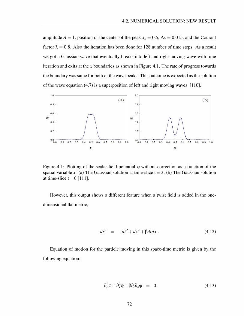
4.2. NUMERICAL SOLUTION: NEW RESULT
amplitude A = 1, position of the center of the peak xc = 0.5, ∆x = 0.015, and the Courant
factor λ = 0.8. Also the iteration has been done for 128 number of time steps. As a result
we got a Gaussian wave that eventually breaks into left and right moving wave with time
iteration and exits at the x boundaries as shown in Figure 4.1. The rate of progress towards
the boundary was same for both of the wave peaks. This outcome is expected as the solution
of the wave equation (4.7) is a superposition of left and right moving waves [110].
Figure 4.1: Plotting of the scalar field potential ϕ without correction as a function of thespatial variable x. (a) The Gaussian solution at time-slice t = 3; (b) The Gaussian solutionat time-slice t = 6 [111].
However, this output shows a different feature when a twist field is added in the one-
dimensional flat metric,
ds2 = −dt2 +dx2 +βdtdx . (4.12)
Equation of motion for the particle moving in this space-time metric is given by the
following equation:
−∂2t ϕ+∂
2xϕ+β∂t∂xϕ = 0 . (4.13)
72

4.2. NUMERICAL SOLUTION: NEW RESULT
Proceeding in a similar fashion to convert a second order differential equation into two
first order dimensional equations , the above equation can be rewritten as:
∂tΠ = ∂xΦ
∂tΦ = ∂xΠ+(∂xβ)Φ+β∂xΦ , (4.14)
with the redefinition :
Π = ∂tϕ−β∂xϕ
Φ = ∂xϕ . (4.15)
Discretizing the equations (4.14) with the help of the time average operator, the central
spatial derivative operator and the forward time derivative operator, one can write:
Φn+1j −Φn
j
∆t= µt(DxΠ
nj)+µt((Dxβ
nj)Φ
nj)+µt(β
nj(DxΦ
nj))
Πn+1j −Πn
j
∆t= µt(DxΦ
nj) . (4.16)
We have started with the form β= x2(x−1)2 with the boundary condition β|x=0 = 0 and
β|x=1 = 0. As an output, we got two asymmetric wave peaks, split from the initial Gaussian
function, moving away from each other towards the boundaries as shown in Figure 4.2.
Again the rate of the progress remains the same for both of the peaks.
73

4.3. CONCLUSION
Figure 4.2: Plotting of the scalar field potential ϕ with twist term β = x2(x− 1)2 as afunction of the spatial variable x. (a) The Gaussian solution at time-slice t = 3; (b) TheGaussian solution at time-slice t = 6 [111].
Finally, we have taken β = sin2(x2(x− 1)2) with the same boundary conditions as the
prior example. This time we have recorded an interesting behaviour of the wave function.
The Gaussian wave generates two waves, one left and one right moving peak with larger
asymmetry and the peaks approaching the boundaries with different progress rate. In Fig-
ure 4.3, it has been shown that at time slice t = 40, the left moving peak has disappeared
from the frame while the right moving peak is still in the frame. This assymetric nature of
the graphs can be shown for scalar field with the original quantum gravitational shift term
as well. This is a work to appear.
This feature might have consequences for the Hawking radiation at the horizon as dis-
cussed in the reference [63]. The convergence of the output has been verified by taking
different values of ∆x. Starting with ∆x = 0.015, we have taken ∆x/2, ∆x/4, ∆x/8 and
got the same image with different scales. Hence the result is converging. Therefore, these
numerical results confirm that a correction in the metric will have an effect on the scalar
field propagation.
74

4.3. CONCLUSION
Figure 4.3: Plotting of scalar field potential ϕ with twist term β = sin2(x2(x− 1)2) as afunction of the spatial variable x. (a) The Gaussian solution at time-slice t = 3; (b) TheGaussian solution at time-slice t = 6; (c) The Gaussian solution at time-slice t = 25; (d)TheGaussian solution at time-slice t = 40 [111].
4.3 Conclusion
In this chapter, we have seen the loop quantum gravity fluctuations generated in the
coherent states give rise to a correction in the Schwarzschild metric and the correction
induces the asymmetric behaviour of a scalar field in a near horizon limit. Though we
have started our journey with the Schwarzschild space-time, our aim is to find the effect for
the binary black hole system. The correction in the Schwarzschild black hole metric may
not have a significant contribution to the one dimensional scalar field propagation though
the asymmetry might influence processes like Hawking radiation. However, in the higher
dimension, because of the non-linearity of the evolution equations, one can expect a non-
trivial outcome. Also, it would be interesting to find out whether this correction imposes
75

4.3. CONCLUSION
any effect to other types of field propagations. In the next chapter, we will study this
loop quantum gravity fluctuation effect on the vector field propagation in a Schwarzschild
background.
76

Chapter 5
Effect on the Vector Field
Maxwell’s Equations have had a
greater impact on human history
than any ten presidents.
– Carl Sagan
A vector is defined as a physical quantity that has a magnitude as well as direction. If
a vector is defined at each point in a manifold, it is a vector field. In physics, the most
common vector field is the Electromagnetic field which describes the propagation of the
light wave. The electromagnetic field can be described by the Maxwell’s equations which
has been modified by Einstein. Maxwell’s equations can be written in a covariant approach
where the electromagnetic field is characterised by an antisymmetric tensor Fµν as dis-
cussed in Chapter 2. Thus one can interpret the electromagnetic field propagation as a fluid
flow [112]. In reference [64], the electromagnetic field propagation has been discussed for
Reissner-Nordstrom and Schwarzschild black hole, and it has been shown that the black
hole entropy is a consequence of vector field propagation in the black hole background.
However, in this thesis, we will study the quantum gravity correction effect for the electro-
magnetic field propagation in the Schwarzschild black hole background.
We will start this chapter with the tensor description for the electromagnetic field. Then
we will study the behaviour of the electromagnetic field propagation in the Schwarzschild
black hole background. Next we will introduce the quantum corrected Schwarzschild met-
77

5.1. ELECTROMAGNETIC FIELD IN CURVED SPACE-TIME
ric to review the vector field propagation. Our aim is to compare between classical and
semi-classically corrected black hole scenario and look for a distinguishable feature in the
electromagnetic field propagation.
5.1 Electromagnetic Field in Curved Space-Time
Maxwell’s equations are given by the following equations, in natural units [113],
∇ ·E =ρ
ε0,
∇×B =∂E∂t
+µ0J ,
∇ ·B = 0 ,
∇×E = −∂B∂t
, (5.1)
where E is the electric field, B is the magnetic field, ρ is the charge density, J is the current
density, ε0 is the permittivity of the free space and µ0 is the permeability of the free space.
In the covariant description, the antisymmetric Faraday tensor Fµν has been introduced
such that for E = E1i+E2 j+E3k and for B = B1i+B2 j+B3k, in natural unit with c = 1
[47],
Fµν =
0 −E1 −E2 −E3
E1 0 B3 −B2
E2 −B3 0 B1
E3 B2 −B1 0
. (5.2)
The inner product of the Faraday tensor is invariant,
FµνFµν = 2(B2−E2) . (5.3)
Inhomogeneous Maxwell’s equations can be written in covariant forms. From the equa-
78

5.1. ELECTROMAGNETIC FIELD IN CURVED SPACE-TIME
tions (5.1), the first two equations can be expressed as,
∇µFµν = µ0Jν , (5.4)
and the last two equations can be written as,
∇τFµν +∇µFντ +∇νFτµ = 0 . (5.5)
The above equation is known as Bianchi Identity [113].
The antisymmetric property of the Faraday tensor together with equation (5.4) imply
the conservation of charge,
∇µJµ = 0 . (5.6)
On the other hand, equation (5.5) allows us to write the Faraday tensor in terms of a four-
vector potential Aµ [47],
Fµν = ∂µAν−∂νAµ . (5.7)
It is to be noted that in the above equation, we have used the partial derivatives instead
of the covariant derivatives. Particular for this equation, one can replace the covariant
derivatives with the partial derivatives as the extra terms containing the affine connections
will be cancelled out. However, we still have an extra degree of the freedom left: with the
replacement of Aµ→ Aµ + ∂µϕ (where ϕ is an arbitrary scalar potential), there will be no
effect on equation (5.7). Here we need a gauge fixing in order to remove the freedom. Thus,
with an appropriate choice of Lorentz-Gauge condition ∂µAµ = 0 [64], one can simplify
the Maxwell equations as,
Aµ =−µ0Jµ , (5.8)
where the operator “” represents the four-dimensional d’Alembert operator ∂ν∂ν =−∂2t +
∇2. Moreover, Faraday tensor determines the energy-momentum tensor in the electromag-
79

5.2. ELECTROMAGNETIC FIELD PROPAGATION IN SCHWARZSCHILDBACKGROUND
netic field [113],
Tµν =−1µ0
[FµτFτ
ν +14
gµνFαβFαβ
]. (5.9)
Thus we have introduced the electromagnetic field equations in covariant form and now one
can look for the solution of the equations (5.4) and (5.5) in a curved space-time. In the next
section, we solve Maxwell’s equations with the Schwarzschild metric components. In the
Minkowski space-time, these calculations are trivial compared to the curved space-time. In
the curved background, one has to consider the coupling between the electromagnetic field
and the geometry of the space-time. Things get more complicated when the background
metric is non-diagonal, i.e. when the metric has cross-components from the coordinates.
One may need to use numerical methods in order to solve the non-trivial differential equa-
tions.
5.2 Electromagnetic Field Propagation in Schwarzschild Background
Following reference [64], in this section, we will study the electromagnetic field prop-
agation in the Schwarzschild black hole background. Maxwell’s equations will be solved
with the background of Schwarzschild metric and with a semi-classical approximation.
We will start with a coordinate transformation of the spherical coordinates in Schwarzschild
black hole, because a stereo-graphic coordinate is more relevant and easier to deal with for
further calculation. Referring to the Schwarzschild metric in Chapter 2, we have already
seen that, in natural unit with G = 1,
ds2 =−(
1− 2Mr
)dt2 +
(1− 2M
r
)−1
dr2 + r2dθ2 + r2 sin2
θdφ2 . (5.10)
The angular part of the above equation can be redefined as,
dθ2 + sin2
θdφ2 =
4(1+ zz)2 dzdz , (5.11)
80

5.2. ELECTROMAGNETIC FIELD PROPAGATION IN SCHWARZSCHILDBACKGROUND
where z = sinθeiφ
1−cosθand z = sinθe−iφ
1−cosθ. Hence the non-zero metric components are redefined as,
g00 =−(
1− 2Mr
), g11 =
(1
1− 2Mr
),
g23 =2r2
(1+ zz)2 . (5.12)
It is to be noted we have changed the coordinate just to make the equations easily solvable.
This part can be skipped if one is comfortable enough to deal with regular Schwarzschild
coordinate system. Equation (5.4) without any source is,
∇µFµν = 0 . (5.13)
Using the form of Fµν in terms of vector potential, i.e, Fµν = ∇µAν−∇νAµ, one can
obtain,
Aµ−∇ν∇µAν = 0 , (5.14)
where = ∇µ∇µ. It is to be noted that this equation is different from equation (5.8) as we
have not fix our gauge condition yet. We will choose our gauge later in this calculation in
order to make the equations easier to solve.
However, the above equation can be written in terms of affine connection and partial deriva-
tives such that,
LAµ = Aν∂µΓν +2gαβ
Γναµ∂βAν +∂µ∇νAν , (5.15)
where Γν = gαβΓν
αβ, L is the d’Alembert operator acting on functions such that L= 1√
|g|∂µ√|g|gµν∂ν.
81

5.2. ELECTROMAGNETIC FIELD PROPAGATION IN SCHWARZSCHILDBACKGROUND
From equation (5.15), we will get four independent equations for different values of µ,
LA0 = −2Mr2 (∂0A1−∂1A0)+∂0∇νAν , (5.16)
LA1 = −2Mr2
[∂1A1− (g00)2
∂0A0]+
2r2
(1− 2M
r
)A1
+2g23
r(∂2A3−∂3A2)+∂1∇νAν , (5.17)
LA2 = −2z(1+ zz)r2 ∂3A2 +
2g11
r(∂1A2−∂2A1)+∂2∇νAν , (5.18)
LA3 = −2z(1+ zz)r2 ∂3A3 +
2g11
r(∂1A3−∂3A1)+∂3∇νAν . (5.19)
Now it is time to choose a suitable gauge condition and we fix the gauge as A0 = 0. This
choice leads us to write equation (5.16),
∇νAν− 2Mr2 A1 = 0 . (5.20)
After substituting the values of ∇νAν in the equations (5.17), (5.18), (5.19) and doing a
little bit of calculation, one can obtain,
LAr =− 2r2 ∂r(rgrrAr) , (5.21)[
L+ 2z(1+zz)r2 ∂z
]Az =
2grr
r ∂rAz− 2r
(1− 3M
r
)∂zAr , (5.22)[
L+ 2z(1+zz)r2 ∂z
]Az =
2grr
r ∂rAz− 2r
(1− 3M
r
)∂zAr . (5.23)
There will be two sets of possible solutions for the above equations.
A(1) ≡
(0, 0,
1√2l(l +1)ω
∂zΦ,1√
2l(l +1)ω∂zΦ
), (5.24)
A(2) ≡
(0,
√l(l +1)
2ω3Φ
r2 ,grr√
2l(l +1)ω3∂z∂rΦ,
grr√2l(l +1)ω3
∂z∂rΦ
), (5.25)
82
5.3. ELECTROMAGNETIC FIELD PROPAGATION IN CORRECTEDSCHWARZSCHILD BLACK HOLE: NEW RESULT
where Φ(t,r,z,z) = e−iωt f (r)Y lm(z,z) with spherical harmonics [114],
Ylm = (−1)m
√2l +1
4π(l +m)!(l−m)!
l!(1+ zz)l ∑
n
(−1)n z(l−n) z(l−m−n)
n!(l−m−n)!(l−n)!(m+n)!. (5.26)
It can be shown that Φ follows the relation [64],
Φ =2grr
r∂rΦ . (5.27)
So, we have two possible vector field forms in a Schwarzschild black hole background. In
the next section we will deal with the vector field in the corrected black hole background.
Motivation:
The correction in the Schwarzschild black hole will perturb the vector field and these per-
turbations can be used to test for stability of the space-time. Given the EHT which will
try to obtain the image of a black hole, we can try to find quantum gravity correction to
the image [115], as that is formed by electromagnetic wave or light deflected off the black
hole field. The corrections might also shed light on the nature of the one loop corrections
to black hole entropy.
5.3 Electromagnetic Field Propagation in Corrected Schwarzschild Black
Hole: New Result
The quantum gravity correction, we have computed in the last section, is,
gtr =±21
1− f 2
(rg
r
)3/2t f(
Per
Ser
). (5.28)
For our convenience, we would redefine the correction term as
F(r,θ) =12
gtr =± 11− f 2
(rg
r
)3/2t f(
Per
Ser
). (5.29)
83

5.3. ELECTROMAGNETIC FIELD PROPAGATION IN CORRECTEDSCHWARZSCHILD BLACK HOLE: NEW RESULT
For this calculation, we would not redefine the angular part of the metric as we did in
the last section. Except that part, the calculation for the corrected Schwarzschild metric is
quite straight-forward and will follow the same manner as the last section. From equation
(5.15) with the gauge A0 = 0, we would get the following equations,
∂0
[∇ jA j− 2M
r2 Ar
]= r−2M
r3∂F∂θ(∂1A2−∂2A1) , (5.30)
∂r(∇ jA j)+(∂tAr)MF(r,θ)r(r−2M) +Ar
2(r−2M)r3
+ 2r3 (∂θAθ)+(∂tAθ)
∂F∂θ
1r(r−2M) +Aθ
2cotθ
r3 + 2r3 sin2
θ(∂φAφ) = 0 , (5.31)
∂θ(∇ jA j)− (∂tAr)∂F∂θ
+ 2Fr (∂tAθ)
−2(r−2M)r2 (∂θAr−∂rAθ)+
2cotθ
r2 sin2θ(∂φAφ)+
csc2 θ
r2 Aθ = 0 , (5.32)
∂φ(∇ jA j)+ 2Fr (∂tAφ−∂φAt)
+2(r−2M)r
[cotθ(∂rAφ)− 1
r (∂φAr)]+ 2cotθ
r
[(∂θAφ)− 1
r (∂φAθ)]= 0 . (5.33)
We have ignored higher order terms of F(r,θ) because of their negligible contributions
to the correction. As we can see here, there are some extra terms presented in the above
equations due to the non-zero value of F(r,θ). With the approximation F(r,θ)→ 0 and with
the redefined angular part of the metric, these equations will coincide with the equations
(5.16), (5.17), (5.18) and (5.19). However, the solution of the above equations will be
non-trivial, as expected. It might be numerically solvable.
We initially try to solve the equations near the horizon, that is set r ≈ 2m as the correc-
tion is important near the horizon. That solves equation (5.30) as
∇ jA j− 2mr2 Ar =
r−2mr3
∂F∂θ
∫(∂rAθ−∂θAr) dt + f (r,θ,φ) = Π(r, t,θ) , (5.34)
where we can set f (r,θ,φ) to zero. Using this we can substitute ∇ jA j in other equations,
and assuming that A(r,θ) is independent of φ as the metric is independent of φ. Equation
84

5.3. ELECTROMAGNETIC FIELD PROPAGATION IN CORRECTEDSCHWARZSCHILD BLACK HOLE: NEW RESULT
(5.31) gives,
∂r
(2Mr2 Ar +Π
)+∂tArλg1 +∂θAθ
(2r3
)+∂tAθλg2 +2
cotθ
r3 Aθ = 0 . (5.35)
Similarly, equation (5.32) is
∂θ
(2Mr2 Ar +Π
)−∂tArλg3 +∂tAθλg4 +
csc2 θ
r2 Aθ = 0 , (5.36)
and equation (5.33) is
λg4(∂tAφ)+2cotθ
r∂θAφ = 0 . (5.37)
In the above, λ has been identified as the semi-classical parameter t and
g1 =MF
λr(r−2M), (5.38)
g2 =∂F∂θ
1λr(r−2M)
, (5.39)
g3 =1λ
∂F∂θ
, (5.40)
g4 =1λ
2Fr
. (5.41)
As equation (5.33) is decoupled from Ar, we use equations (5.31) and (5.32) to analyse
the system. We introduce an ansatz for the solution that Ar = A0r +λAr and Aθ = A0
θ+λAθ.
Then the order λ terms from equations (5.31) and (5.32) can be easily isolated. Therefore,
from equation (5.31), we get,
λ
[∂r
(2Mr2 Ar
)+∂θAθ
2r3 +
2cotθ
r3 Aθ + p(t,r,θ)]= 0 , (5.42)
and from (5.32), we get,
λ
[2Mr2 ∂θAr +
csc2 θ
r2 Aθ +h(t,r,θ)]= 0 , (5.43)
85

5.3. ELECTROMAGNETIC FIELD PROPAGATION IN CORRECTEDSCHWARZSCHILD BLACK HOLE: NEW RESULT
where again we have redefined,
p(t,r,θ) = g1∂tA0r +g2∂tA0
θ+∂rΠ , (5.44)
h(t,r,θ) = −g3∂tA0r +g4∂tA0
θ+∂θΠ . (5.45)
Values of A0r and A0
θcan be taken from the equation (5.24) as non-perturbed solutions.
Therefore we can solve for Aθ from equation (5.43) and insert it in equation (5.42) to solve
for Ar. The equation is of the form,
r3
4m∂r
(2mr2 Ar
)−∂θ
(sin2
θ∂θAr)− cosθsinθ∂θAr = Λ(t,r,θ) , (5.46)
where Λ(r, t,θ) is
Λ(r, t,θ) =r2
rg∂θ
(sin2
θ h(r, t,θ))+
r2
rgcosθsinθ h(r, t,θ)− p(r, t,θ) . (5.47)
Next from the RHS of the equation we formulate Ar = A(r)Θ(θ), where Θ(θ) is an
eigenstate of the angular operator with eigenvalue λ. Note this is not the same as the
Legendre polynomial, but can be solved in terms of them. The equation has the form,
r3
4m∂r
(2mr2 A(r)
)− λA(r) =
1Θ(θ)
Λ(t,r,θ) . (5.48)
Given the form of the solution in the zeroth order as by equation (5.24), we can put A0r = 0.
In addition, if we choose θ = π/2 we get for the non-zero term in Λ(r, t),
Λ(r, t) =r2
rg∂θ
(g4∂tA0
θ
)+
r2
rg∂
2θ Π
=
[r2
rgg4∂θ∂t A0
θ+
r2
rg∂
2θ
(r− rg
r3∂F∂θ
∫∂rA0
θdt)]
θ= π
2
. (5.49)
This can be solved for any value of θ. However, from the solution (5.24), the A0θ
is non-
86

5.3. ELECTROMAGNETIC FIELD PROPAGATION IN CORRECTEDSCHWARZSCHILD BLACK HOLE: NEW RESULT
zero near the horizon. If we take as the solution A0θ= eiωr∗eiωt∂zYlm(z,z) with r∗ = r +
2M ln | r2M −1|, again for simplicity, then the above reduces to,
Λ(r, t) =r2
rg
2Fr(iω)eiωteiωr∗
∂θ∂zYlm(z,z)+2r− rg
rrg∂
2θF
∫(iω)
dr∗
dreiωteiωr∗
∂θ∂zYlm(z,z) dt .
(5.50)
We use those values of l, m for which the above equation is non-zero at θ = π
2 . We also
have an estimate for the Φ field in this limit. Φ∼ e−iωte±iωr∗ . Using this we can estimate a
solution at some constant θ = c, and time t = τc as,
dAdr− (1+ λ)
2Ar
=2
rΘ(c)Λ(τc,r,c). (5.51)
This is a first order equation, which can be solved. The solution for A(r) is obtained as,
A(r) = r2(1+λ)∫ 2
rr−2(1+λ) Λ
Θdr . (5.52)
Using various values of λ a plot of the above gives us a non-trivial A(r), though this wave’s
magnitude is small, it can be large near the horizon. The integral is comprised of several
terms which can be computed using Maple. We are showing one of the terms of A(r) in
the Figure 5.1 for λ = 0. From the Figure, it is obvious that the term A(r) has a non-
trivial contribution near the horizon. Even though the effect faded far from the horizon,
it might not give the same result for other values of λ. It is to be noted that this graph is
not multiplied by the semi-classical parameter. Therefore the effect would be infinitesimal
over all. However, the presence of the other modes of perturbation might generate a chaotic
behaviour of the vector field that can be observed using EHT.
We can also get a solution for the angular part Θ. The equation for Θ is can be obtained
from equation (5.46)
sin2θ
d2Θ
dθ2 +3sinθcosθdΘ
dθ− λΘ = 0 . (5.53)
87

5.3. ELECTROMAGNETIC FIELD PROPAGATION IN CORRECTEDSCHWARZSCHILD BLACK HOLE: NEW RESULT
Figure 5.1: A(r) vs. r for λ = 0 [116]
If we redefine Θ = (sinθ)−1Θ, then the equation for Θ is
sin2θ
d2Θ
dθ2 + sinθcosθdΘ
dθ+(2sin2
θ− (1+ λ))Θ = 0 . (5.54)
This equation is in a form of Legendre differential equation [117], hence can be solved in
terms of Legendre polynomial pl(cosθ) with,
l(l +1) = 2 , (5.55)
m2 = 1+ λ . (5.56)
The above equation can be solved for different values of θ and λ. This work is still in
progress. In experiment, we usually fix θ in order to observe the system in an equitorial
plane. Therefore, with constant θ, the solution for Θ should modify the perturbation with
a constant factor. However, it might be important to note the value of θ, for which the
88

5.4. CONCLUSION
perturbation is significant.
5.4 Conclusion
In this Chapter, we studied the behaviour of the electromagnetic field in the semi-
classically corrected background. We find that the quantum fluctuations induce a non-zero
Ar in the solution, and this can influence the computation of one loop corrections to the
black hole entropy [64]. We have approximated our system for calculation convenience.
However, without any approximation, the solution is quite complicated and the perturba-
tion effect might generate an instability in the system. This effect can be tested by using
numerical analysis. At this point, we can conclude that, even with the approximations, the
quantum corrected Schwarzschild black hole is affecting the vector field; therefore, one can
assure the quantum gravity correction effect with a suitable experimental design like EHT.
Research on this topic is on progress. In the next chapter, we will discuss the correction
effect in the tensor field propagation.
89

Chapter 6
Conclusion
The research on quantum gravity is significantly important, especially in this current era
when LIGO has detected the strain produced by a gravity wave in the order of 10−21 [7].
The quality of the experimental set-up is improving fast with time. Therefore, we are
looking forward to build an advanced technology that can detect even smaller changes in
the system.
In this thesis, our aim was to get an observable quantum gravity effect that can verify
the theory itself. We have studied the quantum gravity effect in the scalar, vector and
tensor fields propagation in the semi-classically corrected black hole background. In the
first three chapters, we have discussed the background theories that have been used in the
calculations. After a brief introduction in Chapter 1, we started with the classical gravity
theory in Chapter 2. The important outcome from this chapter was the Schwarzschild black
hole solution. This solution is significant in this thesis, as we have taken our background
space-time to be a Schwarzschild space-time in the later chapters. In Chapter 3, we have
discussed basic canonical formulation of gravity and loop quantum gravity, which was our
main framework to calculate the corrections in the classical Schwarzschild black hole.
The main work of this thesis begins with the quantum correction calculation in Chapter
3. In the classical Schwarzschild space-time, we got a correction generated from the co-
herent states of the loop quantum gravity variables. The effect of this correction has been
studied for the scalar field propagation near the horizon of the black hole in Chapter 4. As a
result, we found that the symmetry will be broken for a scalar ingoing and outgoing modes
90

6.1. WORK IN PROGRESS: EFFECT ON GRAVITATIONAL WAVE IN CORRECTEDBLACK HOLE BACKGROUND
at the horizon; not only that, the propagation velocity will be affected as well. This result
implies that, the quantum gravity correction will have a significant effect on the scalar field.
In the next chapter, we studied the correction effect on the vector field propagation with
the corrected Schwarzschild background. Here, we ended up with an extra correction term
in the form of a radial component of the vector potential which is zero for the classical
Schwarzschild background.
6.1 Work in Progress: Effect on Gravitational Wave in Corrected Black
Hole Background
Gravitational waves are vaccum solutions of the linearized Einstein equations with
tansverse-traceless gauge as described in references [118, 119]. If we consider the weak
gravitational field where our curved metric can be decomposed into the flat Minkowski met-
ric such that gµν = ηµν+hµν+O([hµν]2) with a small perturbation |hµν|<< 1, the perturbed
Ricci tensor can be written as [119],
Rµν =12(hµ
α,να +hν
α,µα−hµν,α
α−h,µν)+O([hµν]2) ,
where h ≡ hαα = ηµαhµα is the trace of the metric perturbations. With the transverse-
traceless gauge [120], the linearized Einstein equation can be expressed as,
hµν = 0 . (6.1)
It can shown that gravitational wave solutions of equation (6.1) are [119] ,
hµν = ℜAµν exp(iκαxα) , (6.2)
91

6.1. WORK IN PROGRESS: EFFECT ON GRAVITATIONAL WAVE IN CORRECTEDBLACK HOLE BACKGROUND
with null four-vector κα and amplitude tensor
Aµν ≡
0 0 0 0
0 Axx Axy 0
0 Axy −Axx 0
0 0 0 0
. (6.3)
In this thesis, our aim was to study the effect of quantum corrections on tensor fields,
or gravity waves. For that purpose, we take the Schwarzschild metric, and study gravity
waves in that. We then resolve the gravity wave propagation in the quantum corrected
metric. Gravitational wave solutions with Schwarzschild black hole background can be
expressed as odd parity perurbation solution under Regge-Wheeler gauge [121] and even
parity perturbation solution under Zerilli gauge [122] as shown in reference [119]. These
solutions are constrained by the Birkhoff’s theorem [123, 124] where the solutions are
spherically symmetric and asymptotically flat. However, if we consider the gravitational
wave solutions with corrected Schwarzschild background, the solutions are not restricted
by the Birkhoff’s theorem. Therefore, we find difficulties in computing the modes of the
gravitational wave. We found that the Einstein equation takes the form,
δRµν = gβα∇β∇νhµα +gβα
∇β∇µhνα−gβα∇β∇αhµν = 0 . (6.4)
where δRµν is the difference between the Ricci tensor associated with corrected Schwarzschild
metric and that of the original Schwarzschild metric. If we calculate equation (6.4) explic-
itly with Regge-Wheeler gauge, there will be no contribution from the components δR00,
δR01 and δR02. However, there will be contributions from the components δR03 and δRi j.
92

6.1. WORK IN PROGRESS: EFFECT ON GRAVITATIONAL WAVE IN CORRECTEDBLACK HOLE BACKGROUND
The general expressions for R0i and Ri j are given by,
δR0i = −gαβ∇β∇ih0α +gαβ
∇β∇0hαi−gαβ∇α∇βh0i
= g00∇0∇ih00 +g01
∇0∇ih01 +g01∇0∇0hi1−g01
∇0∇ih0i
g10∇1∇ih00 +g11
∇1∇ih01 +g11∇1∇0hi1−g11
∇1∇1h0i
g22∇2∇ih02 +g22
∇2∇0hi2−g22∇2∇2h0i
g33∇3∇ih30 +g33
∇3∇0hi3−g33∇3∇3h0i (6.5)
and,
δRi j = −gαβ∂β∂ihα j−gαβ
∂β∂ jhαi +gαβ∂α∂βhi j +gαβ
Γτ
iβ∂τhα j
+ gαβΓ
τ
β j∂τhαi +gαβΓ
τ
αβ∂ihτ j +gαβ
Γτ
αβ∂ jhτi
−gαβΓ
λ
αβ∂λhi j−gαβ
Γλαi∂βhλ j−gαβ
Γλα j∂βhiλ
+2gαβ∂β(Γ
λi jhαλ)−gαβ
Γτ
βiΓλτ jhαλ
−gαβΓ
τ
β jΓλτihαλ−2gαβ
Γτ
αβΓ
λi jhτλ +gαβ
ΓλαiΓ
τ
β jhλτ
+gαβΓ
λα jΓ
τ
βihλτ . (6.6)
Our calculations though are inconclusive at this stage, we will discuss the implications of
the new result obtained. As we can see, the above equations (6.5) and (6.6) are quite
complicated to solve explicitly. For the non-zero components of δRµν, the solutions are ex-
pected to be non-trivial. The complete scenario with both of the odd-parity and even-parity
perturbation may generate a complex situation. If we keep the odd parity waves, we find
that δR11 and δR22 are zero, δR23 and δR13 are non-trivial and signify parity mixing. In the
expression for δR13, we have terms −g01∂21h03 where g01 has a sinθ that changes the parity
of the expression. This will thus mix with δR13 from the even perturbations. This calcu-
lation is very cumbersome to follow. We hope to make progress using suitable computer
software or coding which we are still developing. The use of Zerilli’s equation, or Regge-
93

6.1. WORK IN PROGRESS: EFFECT ON GRAVITATIONAL WAVE IN CORRECTEDBLACK HOLE BACKGROUND
Wheeler’s equation is restricted in this calculation. We find that we have to recalculate the
system and obtain gauge invariant equations similar to the computations of Moncreif [125]
for quantum fluctuations, which are not restricted to the spherical sector.
It is to be noted that we have computed the correction for the Schwarzschild black hole
space-time, which is not a realistic version of actual black holes that exist in the universe. It
would be more interesting to find a correction for Kerr black hole (black hole with rotation)
and binary black hole system (two black holes revolving around each other). However,
we have started the calculation with the simplest space-time and then we can proceed step
by step to find a similar correction for a Kerr black hole followed by a binary black hole
system.
There are different future research plans that can be carried on further. Few of the
important plans are listed below.
• Implement the correction for the binary black hole collapse and study the effect.
• Calculation of the holonomy correction and corrections in all the corresponding mo-
menta in spherical reduced phase space.
• Study the correction effect on gravitational wave emitted from different black holes
and predict the nature of the black holes.
• The quantum gravity strain is of order (10−125) which is very much similar to the
order of the cosmological constant, research can be carried out to explore this coin-
cidence.
• The event horizon telescope will be functional soon, and we can use the equations
studied in this thesis to predict the behaviour of a ‘image of the spherical black hole.’
Some of the above mentioned research projects are already in progress and hopefully the
results will be presented in the very near future.
94

Bibliography
[1] J.B. Hartle. Gravity: An Introduction to Einstein’s General Relativity. Addison-Wesley, 2003.
[2] Newtonian constant of gravitation, 2014. CODATA,http://physics.nist.gov/cgi-bin/cuu/Value?bg.
[3] Chris Pollock. Mercury’s perihelion. http://www.math.toronto.edu/
˜colliand/426_03/Papers03/C_Pollock.pdf.
[4] Albert Einstein. Explanation of the Perihelion Motion of Mercury from the Gen-eral Theory of Relativity. Sitzungsber. Preuss. Akad. Wiss. Berlin (Math. Phys.),1915:831–839, 1915.
[5] Avery E. Broderick, Ramesh Narayan, John Kormendy, Eric S. Perlman, Marcia J.Rieke, and Sheperd S. Doeleman. The Event Horizon of M87. Astrophys. J.,805(2):179, 2015.
[6] Albert Einstein. Uber Gravitationswellen. Sitzungsber. Preuss. Akad. Wiss. Berlin(Math. Phys.), 1918:154–167, 1918.
[7] B. P. Abbott and et al. Gw151226: Observation of gravitational waves from a 22-solar-mass binary black hole coalescence. Phys. Rev. Lett., 116:241103, Jun 2016.
[8] J. Surdej, C. Delacroix, P. Coleman, M. Dominik, S. Habraken, C. Hanot, H. LeCoroller, D. Mawet, H. Quintana, T. Sadibekova, and D. Sluse. The Optimal Gravi-tational Lens Telescope. The Astronomical Journal, 139:1935–1941, May 2010.
[9] Neil Ashby. Relativity in the Global Positioning System. Living Rev. Rel., 6:1, 2003.[100 Years Of Relativity : space-time structure: Einstein and beyond, 257 (2005)].
[10] Joachim Wambsganss. Gravitational lensing in astronomy. Living Rev. Rel., 1:12,1998.
[11] Richard Massey, Thomas Kitching, and Johan Richard. The dark matter of gravita-tional lensing. Rept. Prog. Phys., 73:086901, 2010.
[12] Steven Weinberg. Cosmology. Oxford, UK: Oxford Univ. Pr. (2008) 593 p, 2008.
[13] Kurt Godel. An Example of a new type of cosmological solutions of Einstein’s fieldequations of graviation. Rev. Mod. Phys., 21:447–450, 1949.
95

BIBLIOGRAPHY
[14] M. S. Morris, K. S. Thorne, and U. Yurtsever. Wormholes, Time Machines, and theWeak Energy Condition. Phys. Rev. Lett., 61:1446–1449, 1988.
[15] J. F. Hawley and K. A. Holcomb. Foundations of modern cosmology. New York:Oxford University Press, 1998.
[16] H. Kragh. Quantum Generations; A History Of Physics In The Twentieth. OrientLongman Limited, 2002.
[17] Max Planck and Max Planck. Planck’s Original papers in quantum physics / anno-tated by Hans Kangro ; translated by D. ter Haar and Stephen G. Brush. Taylor andFrancis London, german and english ed. edition, 1972.
[18] A. Einstein and J.J. Stachel. Einstein’s Miraculous Year: Five Papers that Changedthe Face of Physics. Princeton paperbacks. Princeton University Press, 2005.
[19] E. Schrodinger. An Undulatory Theory of the Mechanics of Atoms and Molecules.Physical Review, 28:1049–1070, December 1926.
[20] W. Heisenberg. Uber den anschaulichen inhalt der quantentheoretischen kinematikund mechanik. Zeitschrift fur Physik, 43(3):172–198, 1927.
[21] W. Heisenberg. The actual content of quantum theoretical kinematics and mechanics.National Aeronautics and Space Administration (NASA), 1983.
[22] P. A. M. Dirac. The quantum theory of the emission and absorption of radiation. Pro-ceedings of the Royal Society of London A: Mathematical, Physical and EngineeringSciences, 114(767):243–265, 1927.
[23] J. Huston. QCD: Experimental Review. In Particles and fields. Proceedings, Meet-ing of the Division of the American Physical Society, DPF 2011, Providence, USA,August 9-13, 2011, 2011.
[24] Ted Van Duzer and Charles W. Turner. Principles of Superconductive Devices andCircuits, (Second Ed.). Prentice Hall PTR, Upper Saddle River, NJ, USA, 1999.
[25] Shun Lien Chuang. Physics of optoelectronic devices. wiley New York, 1995.
[26] Thaddeus D Ladd, Fedor Jelezko, Raymond Laflamme, Yasunobu Nakamura,Christopher Monroe, and Jeremy L O’Brien. Quantum computers. Nature,464(7285):45–53, 2010.
[27] Alexandre Bresson, Yannick Bidel, Philippe Bouyer, Bruno Leone, Eamon Murphy,and P Silvestrin. Quantum mechanics for space applications. Applied Physics B,84(4):545–550, 2006.
[28] P.C.W. Davies. Does quantum mechanics play a non-trivial role in life? Biosystems,78(1–3):69 – 79, 2004.
96

BIBLIOGRAPHY
[29] Michael E Peskin and Daniel V Schroeder. An Introduction to Quantum Field The-ory; 1995 ed. Westview, Boulder, CO, 1995. Includes exercises.
[30] C. J. Isham. Canonical quantum gravity and the problem of time. In 19th Inter-national Colloquium on Group Theoretical Methods in Physics (GROUP 19) Sala-manca, Spain, June 29-July 5, 1992, pages 0157–288, 1992.
[31] L. Smolin. Three Roads To Quantum Gravity. Science masters series. Basic Books,2002.
[32] Sabine Hossenfelder. Experimental Search for Quantum Gravity. In Workshop onExperimental Search for Quantum Gravity NORDITA, Stockholm, Sweden, July 12-16, 2010, 2010.
[33] Claus Kiefer. Quantum Gravity. In Abhay Ashtekar and Vesselin Petkov, editors,Springer Handbook of Spacetime, pages 709–722. 2014.
[34] Oliver Sim Bruning, Paul Collier, P Lebrun, Stephen Myers, Ranko Ostojic, JohnPoole, and Paul Proudlock. LHC Design Report. CERN, Geneva, 2004.
[35] R. L. Jaffe. The Casimir effect and the quantum vacuum. Phys. Rev., D72:021301,2005.
[36] Arundhati Dasgupta. Quantum Gravity Effects on Unstable Orbits in SchwarzschildSpace-time. JCAP, 1005:011, 2010.
[37] S. W. Hawking. Particle creation by black holes. Communications in MathematicalPhysics, 43(3):199–220, 1975.
[38] F. Belgiorno, S. L. Cacciatori, M. Clerici, V. Gorini, G. Ortenzi, L. Rizzi, E. Rubino,V. G. Sala, and D. Faccio. Hawking radiation from ultrashort laser pulse filaments.Phys. Rev. Lett., 105:203901, 2010.
[39] S. Doeleman. Building an event horizon telescope: (sub)mm VLBI in the ALMAera. In 10th European VLBI Network Symposium and EVN Users Meeting: VLBIand the New Generation of Radio Arrays, page 53, 2010.
[40] A. Einstein. Die grundlage der allgemeinen relativitatstheorie. Annalen der Physik,354(7):769–822, 1916.
[41] Review b: Coordinate systems. http://web.mit.edu/8.02t/www/materials/modules/ReviewB.pdf.
[42] P. S. Wesson. The application of dimensional analysis to cosmology. Space ScienceReviews, 27:109–153, oct 1980.
[43] C.W. Misner, K.S. Thorne, and J.A. Wheeler. Gravitation. Number pt. 3 in Gravita-tion. W. H. Freeman, 1973.
97

BIBLIOGRAPHY
[44] Richard P. Feynman, Robert B. Leighton, and Matthew Sands. The Feynman lec-tures on physics. Vol. 3: Quantum mechanics. Addison-Wesley Publishing Co., Inc.,Reading, Mass.-London, 1965.
[45] S. S. Shapiro and I. I. Shapiro. Gravitational deflection of light. Einstein Online,04:1003, 2010.
[46] Albert Einstein. On the electrodynamics of moving bodies. Annalen Phys., 17:891–921, 1905.
[47] D.J. Griffiths. Introduction to Electrodynamics. Prentice Hall, 1999.
[48] H. Minkowski and V. Petkov. Space and Time: Minkowski’s papers on relativity.Minkowski Institute Press, 2013.
[49] Roger Penrose. The road to reality : a complete guide to the laws of the universe.Vintage, London, 2005.
[50] Susskind L. Lecture notes. http://www.lecture-notes.co.uk/susskind/special-relativity/lecture-4/space-time-separation/.
[51] Sergei A. Klioner. The problem of clock synchronization: A relativistic approach.Celestial Mechanics and Dynamical Astronomy, 53(1):81–109, 1992.
[52] Henry Poincare. On the dynamics of the electron (english translation by Scott Wal-ter). Rendiconti del Circolo Matematico di Palermo, 21:129–176, 1906.
[53] R. Katz. An introduction to the special theory of relativity. Van Nostrand momentumbooks. Published for the Commission on College Physics [by] D. Van Nostrand,1964.
[54] Y. Zhang. Special Relativity and Its Experimental Foundations. Advanced Series onArtificial Intelligence. World Scientific, 1997.
[55] C. Christodoulides. The Special Theory of Relativity: Foundations, Theory, Verifica-tion, Applications. Undergraduate Lecture Notes in Physics. Springer InternationalPublishing, 2016.
[56] Albert Einstein. On the influence of gravitation on the propagation of light. AnnalenPhys., 35:898–908, 1911. [Annalen Phys.14, 425 (2005)].
[57] Sean M. Carroll. Lecture notes on general relativity, 1997. https://inspirehep.net/record/451850?ln=en.
[58] C.J. Isham. Modern Differential Geometry for Physicists. World Scientific lecturenotes in physics. World Scientific, 1999.
[59] B.F. Schutz. A First Course in General Relativity. Series in physics. CambridgeUniversity Press, 1985.
98

BIBLIOGRAPHY
[60] A. Dutta. Parallel transport of a vector on two sphere. Figure is drawn in Xfig, 2016.
[61] A. Dutta. Commutator of covariant derivatives. Figure is drawn in Xfig, 2016.
[62] Jeremy Bernstein. Spontaneous symmetry breaking, gauge theories, the Higgs mech-anism and all that. Rev. Mod. Phys., 46:7–48, Jan 1974.
[63] Daniel Harlow. Jerusalem Lectures on Black Holes and Quantum Information. Rev.Mod. Phys., 88:15002, 2016.
[64] Guido Cognola and Paola Lecca. Electromagnetic fields in Schwarzschild andReissner-Nordstrom geometry. Quantum corrections to the black hole entropy. Phys.Rev., D57:1108–1111, 1998.
[65] Giovanni Modanese and Giorgio Fontana. Effect of the vacuum energy density ongraviton propagation. AIP Conf. Proc., 699:1198, 2004.
[66] Karl Schwarzschild. On the gravitational field of a mass point according to Einstein’stheory. Sitzungsber. Preuss. Akad. Wiss. Berlin (Math. Phys.), 1916:189–196, 1916.
[67] Oas. G. Full derivation of the Schwarzschild solution. http://web.stanford.edu/˜oas/SI/SRGR/notes/SchwarzschildSolution.pdf.
[68] Roger Penrose. Gravitational collapse and space-time singularities. Phys. Rev. Lett.,14:57–59, Jan 1965.
[69] Claes Uggla. Spacetime Singularities: Recent Developments. In Proceedings, 13thMarcel Grossmann Meeting on Recent Developments in Theoretical and Experimen-tal General Relativity, Astrophysics, and Relativistic Field Theories (MG13): Stock-holm, Sweden, July 1-7, 2012, pages 59–79, 2015.
[70] S. Chandrasekhar. On stars, their evolution and their stability. Rev. Mod. Phys.,56:137–147, Apr 1984.
[71] G. ’t Hooft. Perturbative quantum gravity. Subnucl. Ser., 40:249–269, 2003.
[72] K. Becker, M. Becker, and J.H. Schwarz. String Theory and M-Theory: A ModernIntroduction. Cambridge University Press, 2006.
[73] R. Gambini and J. Pullin. A First Course in Loop Quantum Gravity. OUP Oxford,2011.
[74] Carlo Rovelli. Loop quantum gravity. Phys. World, 16N11:37–41, 2003.
[75] Bryce S. DeWitt. Quantum Theory of Gravity. 1. The Canonical Theory. Phys. Rev.,160:1113–1148, 1967.
[76] Bryce S. DeWitt. Quantum Theory of Gravity. 2. The Manifestly Covariant Theory.Phys. Rev., 162:1195–1239, 1967.
99

BIBLIOGRAPHY
[77] Bryce S. DeWitt. Quantum Theory of Gravity. 3. Applications of the CovariantTheory. Phys. Rev., 162:1239–1256, 1967.
[78] Carlo Rovelli and Lee Smolin. Knot theory and quantum gravity. Phys. Rev. Lett.,61:1155–1158, Sep 1988.
[79] A. Ashtekar. New Variables for Classical and Quantum Gravity. Phys. Rev. Lett.,57:2244–2247, 1986.
[80] R. Arnowitt, S. Deser, and C. W. Misner. Dynamical structure and definition ofenergy in general relativity. Phys. Rev., 116:1322–1330, Dec 1959.
[81] R.M. Wald. General Relativity. University of Chicago Press, 1984.
[82] Thomas Thiemann. Modern canonical quantum general relativity. Cambridge Uni-versity Press, 2008.
[83] R. K. P. Zia, E. F. Redish, and S. R. McKay. Making sense of the Legendre transform.American Journal of Physics, 77:614–622, July 2009.
[84] David L. Wiltshire. An Introduction to quantum cosmology. In Cosmology: ThePhysics of the Universe. Proceedings, 8th Physics Summer School, Canberra, Aus-tralia, Jan 16-Feb 3, 1995, pages 473–531, 1995.
[85] Edward Anderson. Problem of Time in Quantum Gravity. Annalen Phys., 524:757–786, 2012.
[86] Soren Holst. Barbero’s Hamiltonian derived from a generalized Hilbert-Palatini ac-tion. Phys. Rev., D53:5966–5969, 1996.
[87] M. Ferraris, M. Francaviglia, and C. Reina. Variational formulation of general rela-tivity from 1915 to 1925 “Palatini’s method” discovered by Einstein in 1925. GeneralRelativity and Gravitation, 14:243–254, March 1982.
[88] Giorgio Immirzi. Quantum gravity and Regge calculus. Nucl. Phys. Proc. Suppl.,57:65–72, 1997.
[89] M. A. Clayton. Canonical general relativity: The Diffeomorphism constraints andspatial frame transformations. J. Math. Phys., 39:3805–3816, 1998.
[90] B. Dittrich. Lecture Notes on Quantum Gravity. Informal lectures given at Universityof New Brunswick.
[91] A. Dutta and A. Dasgupta. Edge intersecting surface S. Figure is drawn in Xfig,2016.
[92] Hermann Nicolai, Kasper Peeters, and Marija Zamaklar. Loop quantum gravity: AnOutside view. Class. Quant. Grav., 22:R193, 2005.
100

BIBLIOGRAPHY
[93] A. Dutta and A. Dasgupta. Semi-Classicaly Corrected Gravity and Numerical Rela-tivity. Nova Science Publishers, 2015.
[94] B Dittrich and T Thiemann. Testing the master constraint programme for loop quan-tum gravity: Iv. free field theories. Classical and Quantum Gravity, 23(4):1121,2006.
[95] T. Thiemann and O. Winkler. Gauge field theory coherent states (GCS). 2. Peaked-ness properties. Class. Quant. Grav., 18:2561–2636, 2001.
[96] Brian C Hall. The inverse segal–bargmann transform for compact lie groups. Journalof Functional Analysis, 143(1):98 – 116, 1997.
[97] G.A. Lemaitre and M.A.H. MacCallum. The Expanding Universe. General Relativ-ity and Gravitation, 29:641–680, May 1997.
[98] John D. Barrow and Douglas J. Shaw. The Value of the Cosmological Constant. Gen.Rel. Grav., 43:2555–2560, 2011. [Int. J. Mod. Phys.D20, 2875 (2011)].
[99] Martin Bojowald, Rituparno Goswami, Roy Maartens, and Parampreet Singh. ABlack hole mass threshold from non-singular quantum gravitational collapse. Phys.Rev. Lett., 95:091302, 2005.
[100] T. Piran. Gamma-Ray Bursts as Probes for Quantum Gravity, pages 351–362.Springer Berlin Heidelberg, Berlin, Heidelberg, 2005.
[101] The 3+1 formulation for general relativity. http://laplace.physics.ubc.ca/2010-pi-nr/ref/387n-03-choptuik-3+1-formulation.pdf.
[102] Examples of rnpl-based finite-difference calculations. http://laplace.physics.ubc.ca/People/matt/Software/RNPL_main.html.
[103] Dennis Philipp and Volker Perlick. Schwarzschild radial perturbations in Ed-dington–Finkelstein and Painleve–Gullstrand coordinates. Int. J. Mod. Phys.,D24(09):1542006, 2015.
[104] Edward Seidel and Wai-Mo Suen. Towards a singularity-proof scheme in numericalrelativity. Phys. Rev. Lett., 69:1845–1848, Sep 1992.
[105] Frans Pretorius. Numerical relativity using a generalized harmonic decomposition.Classical and Quantum Gravity, 22(2):425, 2005.
[106] Matthew W. Choptuik. Universality and scaling in gravitational collapse of a mass-less scalar field. Phys. Rev. Lett., 70:9–12, Jan 1993.
[107] K. W. Morton and D. F. Mayers. Numerical Solution of Partial Differential Equa-tions: An Introduction. Cambridge University Press, New York, NY, USA, 2005.
101
BIBLIOGRAPHY
[108] R. Courant, K. Friedrichs, and H. Lewy. On the Partial Difference Equations ofMathematical Physics. IBM Journal of Research and Development, 11:215–234,March 1967.
[109] Luis Lehner. Numerical relativity: A Review. Class. Quant. Grav., 18:R25–R86,2001.
[110] Julius O Smith. Physical audio signal processing. Linear Predictive, 2010.
[111] A. Dutta and A. Dasgupta. Plotting of scalar field potential with one spatial dimen-sion. Figure is drawn in Mathematica, 2016.
[112] Christos G. Tsagas. Electromagnetic fields in curved spacetimes. Class. Quant.Grav., 22:393–408, 2005.
[113] S. Weinberg. Gravitation and cosmology: principles and applications of the generaltheory of relativity. Wiley, 1972.
[114] R. Penrose and W. Rindler. Spinors and Space-Time: Volume 1, Two-Spinor Cal-culus and Relativistic Fields. Cambridge Monographs on Mathematical Physics.Cambridge University Press, 1987.
[115] J.-P. Luminet. Image of a spherical black hole with thin accretion disk. Astronomyand Astrophysics, 75:228–235, May 1979.
[116] A. Dutta and Arundhati Dasgupta. Plotting of A(r) vs. r. Figure drawn in Maple,2016.
[117] D. Zwillinger. Handbook of Differential Equations. Number v. 1. Academic Press,1998.
[118] Nigel T. Bishop and Luciano Rezzolla. Extraction of gravitational waves in numeri-cal relativity. Living Reviews in Relativity, 19(1):2, 2016.
[119] Luciano Rezzolla. Gravitational waves from perturbed black holes and relativisticstars. In Astroparticle physics and cosmology. Proceedings: Summer School, Trieste,Italy, Jun 17-Jul 5 2002, pages 255–316, 2003.
[120] Richard H. Price and Yan Wang. The transverse traceless gauge and quadrupolesources. American Journal of Physics, 76(10):930–933, 2008.
[121] Tullio Regge and John A. Wheeler. Stability of a schwarzschild singularity. Phys.Rev., 108:1063–1069, Nov 1957.
[122] Frank J. Zerilli. Effective potential for even parity Regge-Wheeler gravitational per-turbation equations. Phys. Rev. Lett., 24:737–738, 1970.
[123] R. D’Inverno. Introducing Einstein’s Relativity. Clarendon Press, 1992.
102

6.1. WORK IN PROGRESS: EFFECT ON GRAVITATIONAL WAVE IN CORRECTEDBLACK HOLE BACKGROUND
[124] G.D. Birkhoff and R.E. Langer. Relativity and Modern Physics. Harvard UniversityPress, 1923.
[125] V. Moncrief. Classical and quantum models of strong cosmic censorship. GeneralRelativity and Gravitation, 15:309–314, April 1983.
103

Appendix A
RNPL Programming for NumericalSolution
RNPL program to solve the 1d wave equation with shift term x2(x−1)2
phi tt = phi xx
recast in first order form
pp t = pi xpi t = pp x
where
pp := phi xpi := phi t
The program uses Crank-Nicholson differencing with(implicit) ingoing/outgoing radiation conditions, usingO(h2) forward and backwards differences, at the boundaries.
Initial data is a Gaussian for pp with pi = idsignum ∗ pp,where
idsignum = -1, 0, 1→ ingoing, time-symmetric, outgoinginitial data, respectively
———————————————————–Definition of memory size (only needed for Fortran)———————————————————–system parameter int memsiz := 1000000
———————————————————–Definition of parameters and associated default values.
104
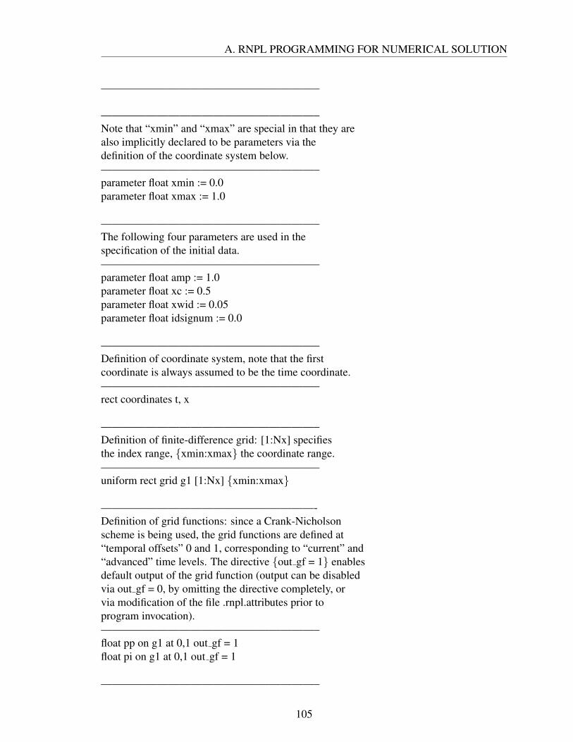
A. RNPL PROGRAMMING FOR NUMERICAL SOLUTION
———————————————————–
———————————————————–Note that “xmin” and “xmax” are special in that they arealso implicitly declared to be parameters via thedefinition of the coordinate system below.———————————————————–parameter float xmin := 0.0parameter float xmax := 1.0
———————————————————–The following four parameters are used in thespecification of the initial data.———————————————————–parameter float amp := 1.0parameter float xc := 0.5parameter float xwid := 0.05parameter float idsignum := 0.0
———————————————————–Definition of coordinate system, note that the firstcoordinate is always assumed to be the time coordinate.———————————————————–rect coordinates t, x
———————————————————–Definition of finite-difference grid: [1:Nx] specifiesthe index range, xmin:xmax the coordinate range.———————————————————–uniform rect grid g1 [1:Nx] xmin:xmax
———————————————————-Definition of grid functions: since a Crank-Nicholsonscheme is being used, the grid functions are defined at“temporal offsets” 0 and 1, corresponding to “current” and“advanced” time levels. The directive out gf = 1 enablesdefault output of the grid function (output can be disabledvia out gf = 0, by omitting the directive completely, orvia modification of the file .rnpl.attributes prior toprogram invocation).———————————————————–float pp on g1 at 0,1 out gf = 1float pi on g1 at 0,1 out gf = 1
———————————————————–
105

A. RNPL PROGRAMMING FOR NUMERICAL SOLUTION
FINITE DIFFERENCE OPERATOR DEFINITIONS———————————————————–———————————————————–Crank Nicholson time derivative operator (first forwarddifference)———————————————————–operator DCN(f,t) := (< 1 > f [0]−< 0 > f [0])/dt
———————————————————–Forward time averaging operator———————————————————–operator MU(f,t) := (< 1 > f [0]+< 0 > f [0])/2
———————————————————–O(h2) centred spatial derivative operator———————————————————–operator D0(f,x) := (< 0 > f [1]−< 0 > f [−1]) / (2∗dx)
———————————————————–O(h2) backwards spatial derivative operator———————————————————–operator DB(f,x) := (3∗< 0 > f [0]−4∗< 0 > f [−1]+< 0 > f [−2]) / (2∗dx)———————————————————–O(h2) forwards spatial derivative operator———————————————————–operator DF(f,x) := (−3∗< 0 > f [0]+4∗< 0 > f [1]−< 0 > f [2]) / (2∗dx)
———————————————————–DIFFERENCE EQUATION DEFINITIONS———————————————————–evaluate residual pp[1 : 1] := DCN(pp,t) = MU(DF(pp,x),t) + MU(DF((x ∗ x) ∗ ((x− 1) ∗ (x− 1)),x)*pp,t) +MU((x∗ x)∗ ((x−1)∗ (x−1))*DF(pp,x),t);[2 : Nx−1] := DCN(pp,t) = MU(D0(pi,x),t) + MU(D0((x ∗ x)∗ ((x−1)∗ (x−1)),x)*pp,t)+ MU((x∗ x)∗ ((x−1)∗ (x−1))*D0(pp,x),t);[Nx : Nx] := DCN(pp,t) = MU(-DB(pp,x),t) + MU(DB((x ∗ x)∗ ((x−1)∗ (x−1)),x)*pp,t)+ MU((x∗ x)∗ ((x−1)∗ (x−1))*DB(pp,x),t);
evaluate residual pi[1 : 1] := DCN(pi,t) = MU(DF(pi,x),t);[2 : Nx−1] := DCN(pi,t) = MU(D0(pp,x),t);[Nx : Nx] := DCN(pi,t) = MU(-DB(pi,x),t);
106

A. RNPL PROGRAMMING FOR NUMERICAL SOLUTION
———————————————————–INITIALIZATION STATEMENTS———————————————————–
———————————————————–Intialize to an ingoing,outgoing or time-symmetricgaussian pulse (in the spatial derivative of the scalarfield), dependent on the value of idsignum.———————————————————–initialize pp[1 : Nx] := amp ∗ exp(-(x-xc)ˆ2/xwidˆ2)initialize pi[1 : Nx] := idsignum ∗ amp ∗ exp(-(x-xc)ˆ2/xwidˆ2)
auto initialize pp, pi
———————————————————–Definition of type of time stepping algorithm. The useof “iterative” here, combined with the “auto update ...”statement below, results in a scheme whereby theresiduals defined above are iteratively relaxed usinga point-wise Newton-Gauss-Seidel technique, until theresidual norms are below a certain threshold.———————————————————–looper iterative
———————————————————–The following statement directs RNPL to automaticallygenerate code to update the grid functions using theresidual definitions.———————————————————–auto update pp, pi
107