Vector Median Filters

Vector Median Filters

Two nonlinear algorithms for processing vector-valued signals are introduced. These algorithms, called vector median operations, are derived from two multidimensional probability density functions using the maximum likelihood estimate approach. The underlying probability densities are exponential and the resulting operations have properties very similar to those of the median filter. These include zero impulse response and preserving of edges in the vector-valued input signal. The vector median filters also have root signals, as does the median filter. In the vector median approach, the samples of the vector-valued input signal are processed as vectors as opposed to componentwise scalar processing. The vector median operation inherently utilizes the correlation between the signal components giving the filters some desirable properties.

General properties as well as the root signals of the vector median filters are studied. The vector median operation is combined with linear filtering, resulting in filters with improved noise attenuation and filters with very good edge response. An efficient algorithm to implement long vector median filters is presented. The noise attenuation of the filters is discussed and an application to velocity filtering is shown.

I . INTRODUCTION

A. Median Filters

The use of median operation in signal processing was introduced by Tukey [I], [2]. The median filter performs a nonlinear filtering operation where a window moves over asignal andateach pointthemedianvalueofthedatawithin thewindow is taken as the output. Median filtering has some desirable properties that cannot be achieved with linear algorithms.

The impulse response of the median filter i s zero. This property makes its use attractive in suppressing impulsive noise. Median filters are robust and are well suited for data smoothing when the noise characteristics are not known. A stepwise change in a signal passes the median filter unal- tered. This property i s used in applications such as image filtering, where data needs to be smoothed but blurring of the signal edges i s not acceptable.

The median of N scalars xi, i = 1, . * * , N, can be defined as the value xmed such that for all y,

It is known that Xmed can always be chosen as one of the x,. If N is odd, x,,d i s unique, and if N i s even there can be an infinite number of possibilities for &,,d. In the median filters N is chosen to be odd.

Suppose that we have a random sample { xl, . . . , xN} from a population having a biexponential density function

f(x) = 'y e-alx-P1 (2) 2

where CY i s a scaling factor and /3 i s an unknown location parameter. The value of fi maximizing the likelihood function

N L ( P ) = n c e-4x,-P1 (3)

is called the maximum likelihood estimate for /3 based on the random sample {xl, . * , xN). By taking a logarithm of (3) we see that the maximum likelihood estimate i s clearly equal to MED[xl, . . , xN]. The median is thus an optimal estimate of the location parameter /3 in the maximum likelihood sense if the input distribution is double exponential as in (2). In a similar manner the average i s the maximum likelihood estimate for the Gaussian distribution.

The output of a median filter is by definition always one of the input samples within the data window (assuming N isodd).Thus, it is possiblethat the filtered signal i s identical to the original signal. If that i s the case, the signal is said to bea root signal for that particular filter. It has been shown that any finite length signal becomes a root signal if filtered repeatedlywith amedian filter[3].The root signalsof afilter are one of the basic tools used to analyze median filters, as the root signals describe, in a way, the "passband" of the filter. For example, a step i s a root signal for any median filter.

Median filters have been applied to both one- and two- dimensional signal processing. The application areas include speech processing and image enhancement [4]-[81. Many authors have analyzed the statistical and root signal properties of these filters [3], [9]-[19], and some modifications and generalizations of median filters have also been introduced [20]-[27].

r = l 2

B. Vector-Valued Signals

Signals in many applications today consist of several separate components, each carrying information on different properties of the signal. In this paper these signals are

Manuscript received January 13, 1989; revised August 20,1989. The authors are with Tarnpere University of Technology, 33101

IEEE Log Number 9034604. Tarnpere, Finland.

0018-9219/90/0400-0678$01 .OO 0 1990 IEEE

PROCEEDINGS OF THE IEEE, VOL. 78, NO. 4, APRIL 1990

referred to as vector-valued signals. Signals that have only one component are called scalar signals.

Typical examples of vector-valued signals are multispectral satellite images and standard color images in n/ systems. In these cases the different components contain information on different parts of the signal spectrum. Another example of a vector-valued signal i s a signal rep- resenting velocity. In three-dimensional space this signal has three separate components corresponding to velocity components in directions of the three axes.

Let the signal have d components xl(n), * . . , xd(n), d L 1. These components form a vector-valued signal

A natural approach for processing x i s to design a filter Tfor a scalar signal and apply it to each component xi separately. Hence, the filter output y is

This method, however, has some drawbacks. The signal components in real applications are generally correlated and, if each component i s processed separately, this correlation i s not utilized. Recently, increasing attention has been given to processing of vector-valued signals in several applications (see, for example, [28]). Separate processing of vector-valued signals may lead to problems that are not present with scalar signals. This i s shown by two examples.

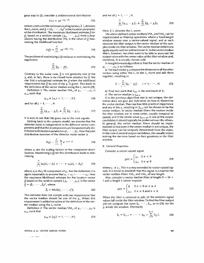
Example 1: Figure 1 shows a color signal with two spectral components, red and green. As a result of the red component havingalowvalueand thegreen component having a high value, the color i s green until the time to where it changes to red. For two time units before to, the red component has a noise impulse, causing the color to be yellow for a duration of one sample. If we apply a median filter of length 5 to both components separately, the impulse in the

result of the filtering the output color will be yellow at the time to before changing to red. Thus the componentwise median filteringof thecolor signal i s not able to remove the false color impulse but only moves its position.

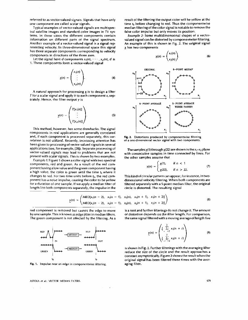
Example 2: Some multidimensional shapes of a vector- valued signal can be distorted by componentwise filtering. An example of this is shown in Fig. 2. The original signal x has two components

(6)

ORIGINAL 5-POINT MEDIAN

I'

5-POINT AVERAGE 5-POINT AVERAGE X*? x2T THREE PASSES

X I I X I -- Fig. 2. Distortions produced by componentwise filtering of a one-dimensional vector signal with two components.

Thesamplesx(l)throughx(22)are shown in thex,-x,plane with consecutive samples in time connected by lines. For the other samples assume that

~ ( l ) , if n < 1 i_ x(22), if n > 22. (7)

This kind of circular pattern can appear,for instance, in two- dimensional velocity filtering. When both components are filtered separately with a 5-point median filter, the original circle i s distorted. The resulting signal

x(n) =

red component is removed but causes the edge to move by one sample.This i s known asedge jitter in median filters. The green component i s not affected by the filtering. As a

IN

4 OUT -

GREEN GREEN ,

'0 '0

Fig. 1. Impulse near an edge in componentwise filtering.

is a root and further filterings do not change it. The amount of distortion depends on the filter length. For comparison, the same signal filtered with a moving average of length five

is shown in Fig. 2. Further filterings with the averaging filter reduce the size of the circle and the result approaches a constant asymptotically. Figure2 shows the resultwhen the original signal has been filtered three times with the averaging filter.

ASTOLA et al.: VECTOR M E D I A N FILTERS 679

Our approach in this paper to processx(n) i s to useafilter - T that regards the samples of I! as vectors

- y(n) = I[x(n)l. (IO)

This way some of the problems caused by componentwise filtering can be avoided.

C. Problem Formulation

To justify and clarify our approach to process vector-valued signals, we present a systems model. This model i s needed in deriving thevector median operation. The signal s;,,(t) shown in Fig. 3 represents the vector-valued phenom-

DETECTOR

: :

Fig. 3. Systems model showing source noise and detector noise components.

enon that i s being observed, for example the velocity of an object. The signal Gs(t) represents noise and undesired vari- ations in the phenomenon itself. We call gs(t) the source noise. The signal

(11)

enters adetector, which decomposes it into dcomponents. Note that this can be done in a number of different ways, and the source noise in the different components of the detector output i s typically not independent. A change in theincoming signal caused bythesourcenoise isverylikely to show in all the components at the same time. The noise components nD(t) represent detector noise that can often be considered independent in the different signal components. The signal coming into the signal processing unit i s then the sum of three components

(12)

We derive algorithms for median-like processing of vector-valued signals using the maximum likelihood estimate approach. For this purpose we make assumptions of the two noise sources and arrive at two vector median algorithms. The choice of the processing method depends on which of the two noise sources i s dominant in a particular system.

One of the two vector median algorithms studied in this paper was among the three median-based location param-

eter estimators of a multispectral distribution compared in [29]. The comparison was based on the estimators' mean square error performance near a multispectral edge; no effort was made to study other properties or the theory of the filters using the algorithm.

D. Outline

Based on the problem formulation given in Section I-C, the vector median i s first defined. General properties resulting from the definition are discussed and it is shown that the vector median has similar properties to the standard median in the scalar case. Also, a generalization of the definition i s presented, making it possible to implement vector median filters optimal for different kinds of input distributions.

In Section I l l , the root signals of the vector median filter are discussed. Theorems characterizing the root signals are presented. In Section IV the vector median operation i s combined with linear filtering. Two methods of doing this are presented. First, an extension to the vector median employing the average of the vectors inside the filter window is defined. This extension improves the noise reduction properties of the vector median filter without losing its nonlinear properties. The second method uses F I R filter substructures and the vector median is computed over the subfilter outputs. Section V discusses the computational aspects of vector median filters. A fast algorithm to implement long vector median filters i s presented. Finally, simulation resultson the noiseattenuation ofthevector median filters and an application to velocity filtering are shown.

I I . VECTOR MEDIAN

When extending the median operation to vector-valued signals, we place some requirements for the resulting vector median operation. First of all, we want the operation to have properties similar to those of the median operation in the scalar case, that is, zero impulse response and good robust data smoothing ability while retaining sharp edges in thesignal. Wealsorequirethat thevector median reduces to the scalar median when the vector dimension i s one.

An important requirement related to a good edge response i s the existence of root signals. Note that if the vector median were defined such that the scalar median operation would be used in each vector component inde- pendently, the vector median filter would have root signals but the output of the filter would not generally be one of the input vectors. One of the basic properties of the median filter i s that it does not introduce any sample values that are not present in the filter input; this should be the case also with the vector median filters. Therefore, we require that the vector median filter output be one of the input vectors.

A. Definition

Consider the two noise sources in the model of Fig. 3, - ns and nD. By assuming exponential distributions for the source and the detector noise and using the maximum likelihood approach, we define two median-like algorithms for processing vector-valued signals.

The source noise in the different components i s dependent and, with no apriori information of the noise, it is reasonable to assume a symmetric distribution. In an analo-

680 PROCEEDINGS OF THE IEEE, VOL. 78, NO. 4, APRIL 1990

gous way to (2), consider a d-dimensional distribution

f(x) = ye-allx-ullz (1 3)

wnereyandaarethe necessaryscalingfactors, 1) 11,denotes the L2 norm, and = (PI, . . . , &)'is the location parameter of the distribution. The maximum likelihood estimate! for - 0, based on a random sample {xl, . . . , xN} from a population having the distribution (13), is the value of maximizing the likelihood function

N

~ ( p ) = n ye-4~3-8112. (14)

The problem of maximizing L(P) reduces to minimizing the expression

,=1

N

11x1 - ell,. (1 5)

Contrary to the scalar case, 6 i s not generally one of the x, and, in fact, there i s no closed form solution for 6. We can find a suboptimal estimate for when the additional requirement that be one of the x , i s given. This leads to the definition of the vector median using the L, norm [29].

Definition 7: The vector median VML, of xl, . . . , x N i s x,, such that

(1 6)

1-1

xVm E { x , l i = 1, * * . , N }

and for all j = 1, , N

It i s easy to see that (16) gives rise to the root signals. Getting back to the systems model, we assume that the

detector noise i s independent in the different vector components and that the dcomponents are biexponentiallydis- tributed with location parameters&, . . . ,&Then the joint distribution function of the detector noise vector i s

where a , are the scaling factors of the component distributions. Maximizing L(P) for this distribution leads to minimizing

N

c (allx; - 011 + . . ' + adlxb - Pdl) (19)

where xi i s the j ' th component of x,. For the definition it i s again reasonable to assume that al = a, = * . . = ad. Now the maximum likelihood estimate for the location vector - 0 based on the random sample { x,, . . . , z N } i s the vector - B = (&, . . . , &)', where

,=1

6, = MEDLX;, . . . , .,"I. (20)

This estimate does not comply with our requirement that the vector median should be one of the x,. When this requirement i s added we arrive at the definition of the vector median using the L1 norm.

, xN is x,, such that

Definition 2: The vector median VML, of xl, . *

x,, E { x , l i = 1, . . . , N} (21 )

and for all 1 = 1, . . . , N

N N

I Ixvm - xi111 5 C I Ix, - x,lll* (22) r = l 1 = 1

Here, 11 I l l denotes the L1 norm. The above-defined vector medians VML, and VML, can be

implemented as filtering operations where a fixed-length window moves over a vector-valued signal, and at each moment the filter output is the vector median of the samples inside the filterwindow. Thevector median definitions applyequallywell for odd and even N. In the vector median filters, however, we often want to be able to associate the output value with the center value of the filter window and, therefore, N is usually chosen odd.

A straightforward algorithm to find the vector median of xl, . . . , x N i s as follows:

a) For each vector E, computethe distances to all theother vectors using either the L, or the L2 norm and add them together, resulting in

N

SI = c Ilx, - x,\l, i = 1, * * , N. (23) / = 1

b) Find rnin such that S,,, i s the minimum of S I . c) The vector median i s x,,,. If in the previous algorithm min i s not unique, the def-

inition does not give any indication on how to determine the vector median. This case has little practical impprtance and any of the x, resulting in S,,, can be chosen to be the vector median. In vector median filters the vectors inside the filter window are in some order, usually temporal or spatial, and if the center value X(N+1)/2 is one of the output candidates it should typically be preferred over the others. In general, the vector median filters should be implemented so that even if thevector median is not unique, the filter output can be uniquely determined from the input. In the case of several output candidates, this usually means making the decision based on their positions in the filter window.

B. General Properties

Consider a vector-valued signal

cl, if n c 0

c,, i f n 2 0 x(n) =

wherecl # c2. This is a step extended to vector-valued signals. It i s trivial to establish that this signal i s a root for the vector median filters VML, and VML2 of any length.

Also, consider a vector median filter of length N = 2k + 1 and a length k vector impulse

When the filter i s centered at x(k ) , all the nonzero signal values fall inside the filter window. To find the filter output y ( k ) we compute the sums so, . , S2k, as in (23), for the X I inside the window. Obviously

k - I

I = o Sk = Sk+l = . . . = SZk = IlCIll. (26)

ASTOLA et al.: VECTOR MEDIAN FILTERS 681

and for all j = 1, . . . , N N N

dist(xgvm - x,) I dist(x_, - x,) (31)

where dist(x, y ) i s the distance between the vectors x and y . The d i st a nce-f u n c t io n depends on the d i s t r i but i on be h i nd it. For example, the generalized vector median derived from the Gaussian distribution uses the distance function

dist(x, y ) = Ilx - ylli. (32)

In [30], a class of median type filters based on the scalar distri bution

, = I , = I

-

f(x) = (ye-lX-01’ (33)

was derived. The generalized vector median concept can be used to extend these filters to vector-valued signals.

(28)

As S k 5 S, for all j = 0, . . . , k - 1, the filter output i s x k

= 0. The vector median filters thus remove impulses in a fashion similar to that of the scalar median filter. In the previous equations, )I II can be replaced either with 11 11, or II I l l , and the result holds for both vector median filters. Note also that no assumptions are made of the signal values eo,

The vector median filters are invariant to scale and bias. t c k - 1 .

. . .

This means that

VM[axl + c, ax , + c, . . . , a x N + r] = aVM[xl, x,, . * . , xhi ] + c. (29)

Here, a i s a scalar and c i s a vector constant. As a rotation of the coordinate system does not affect the L, norm of a vector, the vector median filter VM,, based on that norm is also rotation invariant.

All the above-mentioned properties are similar to the properties of the scalar median, and if the vector dimension is one, both of the vector median definitions reduce to the scalar median definition. Having established this we will concentrate on studying VM,,. Unless otherwise stated, the later references to vector median in this paper are to VML, and the notation VM means VM,,.

We now return to the example in Fig. 1 . If the vector-valued color signal i s filtered with a vector median filter of length 5, the impulse in the red component is removed without the edge jitter. This i s shown in Fig. 4. We will later

D E D R RED 7

GREEN A GREEN b4-0

‘0 ‘0

Fig. 4. Impulse near an edge in vector median filtering.

show by simulation that thisvector median operation based on the L, norm can be used to achieve very good noise reduction near signal edges.

C. Generalized Vector Median

The definitions of VML, and VML, are based on the distributions (13) and (I@, respectively. The same approach can be used to derive vector operations optimal for different input distributions.

Definition 3: The generalized vector median (GVM) of x,, . . . , x N i s the vector xg,, such that

(30) Xgvm E { X , l i = 1, . . . , N )

Ill. ROOT SIGNALS

Avector-valued signalx(n) = { . . . ,x ( - l ) ,g (O) ,z ( l ) , . . . ) is a root signal of the vector median filter of length N = 2k + 1 if for all n

(34)

As the vector median filter response to any input signal i s uniquely defined and the output of the filter is one of the samples in the filter input, it follows that if a finite-length signal i s repeatedlyfiltered with avector median filter it will either become a root signal that is invariant to filtering or itwil l eventually start periodically repeating itself.AIl of our computer simulations of the vector median filters indicate that repeated filterings result in a root signal; we prove this for the case when the filter length i s 3. The proof appears difficult for longer filters.

VM[x(n - k) , . . . , x(n), . . . , x(n + k)] = x(n).

Theorem 7: A vector-valued signal of length L + 2

s = { X o t E l , E,, . . . , X L - l , XL, XL+l) (35)

will turn intoa root signal if filtered repeatedlywith thevector median filter of length 3. The samples x o = xl and x , + ~ = xL have been appended to the signal and the center point of the filter window i s moved from xl to x L .

Proof: Assume that (35) i s a signal that will not turn into a root signal and that it i s the shortest signal of that kind. Repeated filterings of (35) then necessarily produce a periodically recurring sequence of signals with a period K. Lets’be thesignalsafterif i l teringsandsM bethe first signal of the repeating sequence, which is

sM = {Xo, X I , xY, . . . , X Y - I , XL! X L + l J

(36)

First,notethatforalli,xb = & =x1andx; = =x,.Also, if X$ = xl then 8; = X, for all i > j , and because of the peri-


odicity x"' = x,. Thus, (35) could have been replaced with a shorter signal of length L + 1

(37)

From these observations and the definition of the vector median it follows that

M M M 1 x 2 , x 2 I x 3 , . * * ! xY-1, X L ! XL+13.

(38) , + 1 llx, - x 2 II 5 11x1 - x;ll. Considering that &'C/K = x$" for all j L 0, (38) yields

lIxl - &ll = constant (39)

for all i r M. When we take into account that if (17) does not give a unique output vector the center value i s given preference over the others, then we get the result x;+l = &for all i r M. This means that the shorter signal (37) could again have been used to replacetheoriginal signal and there can be nosignalzthatcould producethe periodicsequence (36). Therefore, 5 has to turn into a root signal. This proof holds for both VML, and V M L , when 11 11 i s replaced with the corresponding norm. Note also that the proof is independent of the vector dimensions.

Let us return to the example of Fig. 2. The circle that i s distorted by componentwise filtering i s a root signal of the vector median filters VML, and VML, of length 5. The vector median filter i s also able to preserve many other smooth shapes that are corrupted by componentwise filtering.

Given thecomplexityof characterizingall the rootsofthe standard median filter it seems hopeless to give a complete characterization of the roots of the vector median filter. However, for the most important case of slowly varying signals, it i s possible to give a simple criterion guaranteeing that a signal i s a root signal.

Theorem 2: The signal x(n) i s a root signal of the vector median filter of length N = 2k + 1, k 2 1, if for all n, x(n) satisfies

(x(n) - x(jN . M i ) - x(n))

Ilx(n) - x~j~l1211x~i~ - x(n)l12

k - I k L- (40)

whenever n - k 5 j < n < i 5 n + k. Proof: Let x(n) satisfy (40). We can assume that the center

of the window is at x(k). By symmetry it i s enough to show that

2k 2k

= ,Fo l I X ( i ) - X( j ) l l 2 2 I l X ( i ) - = Sk (41) r = O

Xti)

Fig. 5. Proof of Theorem 2.

By geometrical considerations illustrated in Fig. 5

Mi) - x(i)l12 - Ilx(i) - x(k)II2

I cos a

k - 1

- c IlxW - x(j)l12 = 0 , =o ' + I

(45)

implying the theorem. Note that thecondition (40) i s sufficient but not necessary

for the signal to be a root signal. The condition means that if a linewere drawn through any point in the left part of the filter window and the center point of the window and another line through the center point and any point in the right part of the window, then the angle (Y between these two lines would be small enough to satisfy cos cy 2 1 - 1 /k. The longer the filter the smaller the angle has to be. This kind of condition cannot be derived for VML, because it is not rotation invariant.

It i s known that if a scalar signal i s a root of the median filter of length N it i s also a root of all the shorter median filters [3]. A similar result follows from Theorem 2. If x(n) satisfies (40) and i s thus a root of the vector median filter of length N, then x(n) is also a root of any vector median filter whose length is smaller than N. Note, however, that this applies only to the roots satisfying (40). As Theorem 2 only gave a sufficient condition, it i s possible that there are other kinds of root signals for the filter of length N that are not necessarily roots of all the shorter filters. This is indeed the case: for example, the following vector-valued signal with two vector components is a root of the vector median filter (VML,) of length 5 but i s not a root of the three-point


f i Iter:

IV. COMBINING VECTOR MEDIAN WITH LINEAR FILTERING

A. Extended Vector Median

In some applications the noise attenuation of the vector median operation may prove inadequate. We present an extension combining the vector median operation with an averaging filter. The output of the extended vector median filter i s either the same as that of the corresponding vector median filter or that of an averaging filter of the same length.

Definition 4: The extended vector median (EVM) of xl, . . . , X N i s xeVm such that

f N N

(xvm, otherwise, (46)

where

(47)

We arrive at this definition when minimizing (15) with a constraint that be one of x i or xaVe. The definition is for VM,, but the same extension can be applied to VM,, or to any generalized vector median. Note that this extension is useless in the scalar casewhere, unless it equals the median, the average never appears in the filter output.

Even though the output of the extended vector median filter is not always one of the input samples, the filter inher- its many properties of the vector median filter. The step signal (24) i s a root signal also for the EVM filter of any length and the EVM filter of length N = 2 k + 1 is able tocompletely remove impulsesof length kor less. The EVM filter in a sense adapts to the input signal so that near a signal edge it behaves like the vector median filter and does not blur the edge,whereas in the smooth areas of the signal it more often chooses the average vector to be the output, resulting in improved noise attenuation.

Figure 6 shows some results of computer simulations made to study the decision process of the extended vector

20 5 10 15

Fig. 6. Percentage of averages in the EVM filter output.

FILTER LENGTH

~

median filter in noisyconditions.The inputtotheEVMfilter was r(n) = (x,(n), , xd(n))‘, where the components xi(n) were normally distributed white noise with zero mean and unit variance. Whether filter output was chosen to be gave or x,, was recorded for 10 000 output samples. Figure 6 shows the ratio of averages and all output samples for different filter lengths and input vector dimensions. The results showthat when the filter length and the input vector dimension increase, the EVM filter becomes very close to an averaging filter.

B. Linear Substructures

FIR-median hybrid (FMH) filters were introduced in 1221. They combine linear filtering with the median operation by dividing the filter window into an odd number of smaller subwindows where FIR filters are operating. The FMH filter output i s the median of the FIR filter outputs.

The statistical properties and the root signals of the FIR- median hybrid filters are very similar to thoseof the median filters. The FIR-median hybrid filters, however, offer some obvious advantages compared to the median filter having thesamelength.Thenumberof subfilters isgenerally much smaller than the length of the filter window and finding the median becomes more efficient. Reducing the number of points that median is taken over will also significantly sharpen the edge response of the filter in noisy conditions. FMH filters also allow more design possibilities than the median filter because the subwindows and the corresponding FIR filters are available as design factors [31], [32].

The advantages of the FMH filters are even more important in vector median filtering, where the task of finding the vector median of a large number of input vectors can be cumbersome. Consider an FMH filter of length N = 2 k + 1 with three substructures

+ z’) 1 k

H ~ ( z ) = - (zk + zk - ’ + * *

H & z ) = 1

H3(z) = -! (z-’ + z-* + . . + z - ~ ) . (48)

H, and H3 are averaging filters and the output of H2 i s just a copy of the middle point of the filter window. We use this simple structureto form our basicvector FIR-median hybrid (VFMH) filter. If the input signal i s x(n) the output of the VFMH filter of length N = 2 k + 1 i s

k

Figure 7 shows a block diagram of this filter. The corresponding extended vector FIR-median hybrid (EVFMH) filter is formed by replacing the VM operation with the EVM operation. In these structures the vector median i s computed over three vectors independent of the filter window size. This three-point structure has a very good edge response in noisy conditions and is simple to implement.


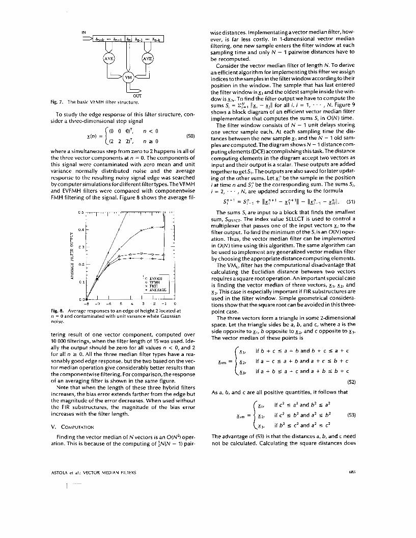
Fig. 7. The basic OUT

VFMH filter structure.

To study the edge response of this filter structure, consider a three-dimensional step signal

g(n) = (0 0 O ) T , n < 0

(50)

where a simultaneous step from zero to 2 happens in all of the three vector components at n = 0. The components of this signal were contaminated with zero mean and unit variance normally distributed noise and the average response to the resulting noisy signal edge was searched by computer simulations for different filter types. TheVFMH and EVFMH filters were compared with componentwise FMH filtering of the signal. Figure 8 shows the average fil-

i (2 2 2)T, n L 0

-8 -7 -6 -5 -4 -3 -2 -1 0

Fig. 8. Average responses to an edge of height 2 located at n = 0 and contaminated with unit variance white Gaussian noise.

tering result of one vector component, computed over 10 000 filterings, when the filter length of 15 was used. Ide- ally the output should be zero for all values n c 0, and 2 for all n 2 0. All the three median filter types have a reasonably good edge response, but the two based on the vector median operation give considerably better results than the componentwise filtering. For comparison, the response of an averaging filter is shown in the same figure.

Note that when the length of these three hybrid filters increases, the bias error extends farther from the edge but the magnitude of the error decreases. When used without the FIR substructures, the magnitude of the bias error increases with the filter length.

V. COMPUTATION

Finding the vector median of N vectors i s an O(N2) operation. This i s because of the computing of jN(N - 1) pair-

wise distances. lmplementatingavector median filter, however, i s far less costly. In l-dimensional vector median filtering, one new sample enters the filter window at each sampling time and only N - 1 pairwise distances have to be recomputed.

Consider the vector median filter of length N. To derive an efficient algorithm for implementing this filter we assign indicestothesamples in the filterwindow accordingto their position in the window. The sample that has last entered the filter window isg, and the oldest sample inside the window i s g,,. To find the filter output we have to compute the sums SI = Ilg, - g,II for all i, i = 1, . * , N. Figure 9 shows a block diagram of an efficient vector median filter implementation that computes the sums S, in O(N) time.

The filter window consists of N - 1 unit delays storing one vector sample each. At each sampling time the distances between the new sample gl and the N - 1 old samples are computed. The diagram shows N - 1 distance computing elements (DCE) accomplishing this task. Thedistance computing elements in the diagram accept two vectors as input and their output i s a scalar. These outputs are added togethertogetS,.Theoutputsarealso saved for later updat- ing of the other sums. Let be the sample in the position i at time n and Sy be the corresponding sum. The sums S I , i = 2, . . . , N, are updated according to the formula

S:+' = S:-i + 1 1 ~ : " - g;+'l( - llgy-1 - &[I. (51)

The sums S, are input to a block that finds the smallest sum, SSELECT. The index value SELECT is used to control a multiplexer that passes one of the input vectors g, to the filter output. To find the minimum of the S, is an O(N) operation. Thus, the vector median filter can be implemented in O(N) time using this algorithm. The same algorithm can be used to implement any generalized vector median filter by choosing the appropriate distancecomputing elements.

The VML, filter has the computational disadvantage that calculating the Euclidian distance between two vectors requires a square root operation. An important special case is finding the vector median of three vectors, gl, g2, and g3. This case is especially important if FIR substructures are used in the filter window. Simple geometrical considerations show that the square root can be avoided in this three- point case.

The three vectors form a triangle in some 2-dimensional space. Let the triangle sides be a, b, and c, where a is the side opposite to gl, b opposite to g,, and c opposite to g3. The vector median of these points i s

gl, i f b + c I a + b a n d b + c I a + c

g,,= g2, i f a + c s a + b a n d a + c s b + c

i f a + b s a + c a n d a + b I b + c g3,

(52)

i AS a, b, and c are all positive quantities, it follows that

g,, if c2 I a2 and b2 I a2 i g3, if b2 I c2 and a2 I c2

g,, = g,, if c2 I. b2 and a2 5 b2 (53)

The advantage of (53) i s that the distances a, b, and c need not be calculated. Calculating the square distances does


IN

I

Fig. 9. Block diagram of the vector median filter algorithm.

not require square root operations. The L, norm is considerably easier to compute than the L 2 norm. Thus this approach is not useful in implementing three-point VML, filters.

VI. SIMULATION RESULTS AND EXAMPLES

A. Noise Attenuation

Mathematical analysis of the statistical properties of the vector median filters leads to difficult expressions. Con- sider the simplest possible case of three independent random vectorsx,,x,, andzg, having the same probabilityden- sity function f(x). The probability density of the output of the three-point vector median filter i s given by the expression

g ( x ) = 3f(x) 1 1 f ( _ v ) f(z) d_v dz (54) R d ( L . 6 )

where d i s the dimension of x, and Rd(y , I) i s the region in the RZd-space where llx - zll I Ily --zII and Ilx - y11 I 1 1 ~ - yll. Usually, f(3) alone is complex enough to make solving g ( x ) very difficult. Furthermore, we are also inter- ested in longer vector median filters and in the extended vector median filters. Therefore, computer simulations were used to study the noise attenuation of the vector median filters.

When the noise is independent in the different vector components, the vector median filters cannot in general achieve the same noise attenuation as the componentwise median filtering because they are under the restriction that the output is one of the vectors inside the filter window. With Gaussian noise the extended vector median filter gives approximately the same noise attenuation as component-

wise median filtering if the vector dimension is small (13) and the filter i s reasonably short (515). When the vector dimension and the filter length increase, the noise attenuation of the extended vector median filter further improves and asymptotically approaches that of an averaging filter. This is in agreement with the results of Fig. 6.

Figure 10 shows the simulation results for the case when the input signal i s white Gaussian noise. Vectors with two components were used and thevarianceof the input signal, that is, the sum of variances of the two components, was 1.0. The output variance for different filter types and filter lengths i s shown. The averaging filter gives the best possible noise reduction for Gaussian noise and is included as a reference. Also included, marked as "optimal GVM," i s

5 10 15 FILTER LENGTH

Fig. 10. Output variance as function of filter length. Input signal is white Gaussian uncorrelated unit variance vector noise. Vector dimension i s 2.


the generalized vector median using the distance function (32). That filter has the best possible Gaussian noise reduction when the output i s required to be one of the inputs. The results show that VML, and VML, are close to optimal under that condition.

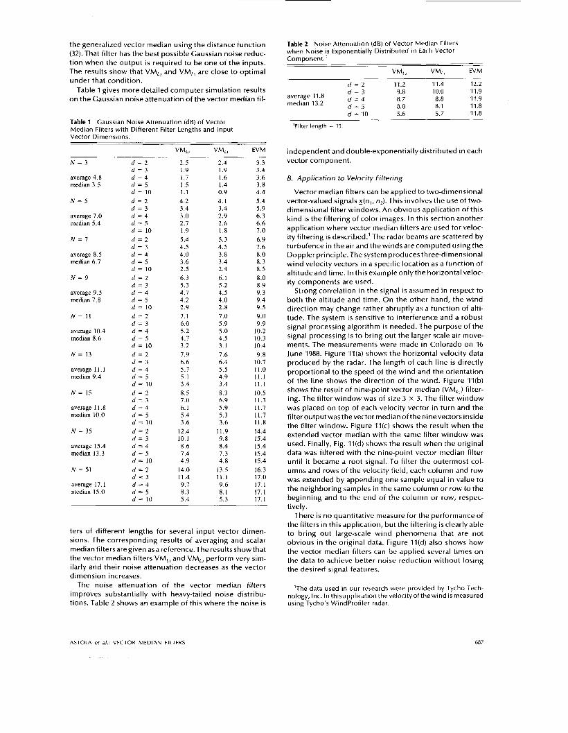
Table 1 gives more detailed computer simulation results on the Gaussian noise attenuation of the vector median fil-

Table l Median Filters with Different Filter Lengths and Input Vector Dimensions.

Gaussian Noise Attenuation (dB) of Vector

N = 3

average 4.8 median 3.5

N = 5

average 7 .O median 5.4

N = 7


N = 9


N = 11


N = 13


N = 15

average 1 1.8 median 10.0

N = 35


N = 51


d = 2 d = 3 d = 4 d = 5 d = 10 d = 2 d = 3 d = 4 d = 5 d = 10 d = 2 d = 3 d = 4 d = 5 d = 10 d = 2 d = 3 d = 4 d = 5 d = 10 d = 2 d = 3 d = 4 d = 5 d = 10 d = 2 d = 3 d = 4 d = 5 d = l O d = 2 d = 3 d = 4 d = 5 d = 10 d = 2 d = 3 d = 4 d = 5 d = 10 d = 2 d = 3 d = 4 d = 5 d = 10

2.5 1.9 1.7 1.5 1.1 4.2 3.4 3.0 2.7 1.9 5.4 4.5 4.0 3.6 2.5 6.3 5.3 4.7 4.2 2.9 7.1 6.0 5.2 4.7 3.2 7.9 6.6 5.7 5.1 3.4 8.5 7.0 6.1 5.4 3.6

12.4 10. I 8.6 7.4 4.9

14.0 11.4 9.7 8.3 5.4

2.4 1.9 1.6 1.4 0.9 4.1 3.4 2.9 2.6 1.8 5.3 4.5 3.8 3.4 2.4 6.1 5.2 4.5 4.0 2.8 7.0 5.9 5.0 4.5 3.1 7.6 6.4 5.5 4.9 3.4 8.3 6.9 5.9 5.3 3.6

11.9 9.8 8.4 7.3 4.8

13.5 1 1 . 1 9.6 8.1 5.3

3.3 3.4 3.6 3.8 4.4 5.4 5.9 6.3 6.6 7.0 6.9 7.6 8.0 8.3 8.5 8.0 8.9 9.3 9.4 9.5 9.0 9.9

10.2 10.3 10.4 9.8

10.7 11.0 11.1 11.1 10.5 11.3 11.7 11.7 11.8 14.4 15.4 15.4 15.4 15.4 16.3 17.0 17.1 17.1 17.1

ters of different lengths for several input vector dimensions. The corresponding results of averaging and scalar median filtersaregiven asa reference.The resultsshowthat the vector median filters VM,, and VM,, perform very sim- ilarly and their noise attenuation decreases as the vector dimension increases.

The noise attenuation of the vector median filters improves substantially with heavy-tailed noise distributions. Table 2 shows an example of this where the noise i s

Table 2 Noise Attenuation (dB) of Vector Median Filters when Noise is Exponentially Distributed in Each Vector Component.’

VM,, VML, EVM

d = 2 11.2 11.4 12.2 9.8 10.0 11.9 8.7 8.8 11.9 8.0 8.1 11.8

d = 10 5.6 5.7 11.8

average 11.8 = median 13.2 f

’Filter length = 15.

independent and double-exponentially distributed in each vector component.

B. Application to Velocity Filtering

Vector median filters can be applied to two-dimensional vector-valued signals x(nl, n2). This involves the use of two- dimensional filter windows. An obvious application of this kind is the filtering of color images. In this section another application where vector median filters are used for velocity filtering i s described.’ The radar beams are scattered by turbulence in the air and the winds are computed using the Doppler principle. The system produces three-dimensional wind velocity vectors in a specific location as a function of altitudeand time. In this exampleonlythe horizontal velocity components are used.

Strong correlation in the signal i s assumed in respect to both the altitude and time. On the other hand, the wind direction may change rather abruptly as a function of altitude. The system is sensitive to interference and a robust signal processing algorithm i s needed. The purpose of the signal processing i s to bring out the larger scale air move- ments. The measurements were made in Colorado on 16 June 1988. Figure I l (a) shows the horizontal velocity data produced by the radar. The length of each line i s directly proportional to the speed of the wind and the orientation of the line shows the direction of the wind. Figure I l ( b ) shows the result of nine-point vector median (VM,,) filtering. The filter window was of size 3 x 3. The filter window was placed on top of each velocity vector in turn and the filteroutputwasthevector median ofthe ninevectors inside the filter window. Figure I l ( c ) shows the result when the extended vector median with the same filter window was used. Finally, Fig. I l ( d ) shows the result when the original data was filtered with the nine-point vector median filter until it became a root signal. To filter the outermost col- umns and rows of the velocity field, each column and row was extended by appending one sample equal in value to the neighboring samples in the same column or row to the beginning and to the end of the column or row, respectively.

There i s no quantitative measure for the performance of the filters in this application, but the filtering is clearly able to bring out large-scale wind phenomena that are not obvious in the original data. Figure I l ( d ) also shows how the vector median filters can be applied several times on the data to achieve better noise reduction without losing the desired signal features.

’The data used in our research were provided by Tycho Tech- nology, Inc. In this application thevelocityof the wind is measured using Tycho’s Windprofiler radar.

ASTOLA et al.: VECTOR M E D I A N FILTERS 687

VII. CONCLUSIONS

A systems model with two separate noise sources was presented, giving rise to two vector median operations. The source noise was assumed to be dependent in the different vector components, leading to the definition of the vector median based on the L 2 norm, whereas the vector median Using the L, norm was based on the detector noise that was q5Sumed to be independent in the different vector components. The vector median operations were derived using the maximum likelihood estimate approach under the constraint that one of the input vectors is chosen to be the output.

In the vector median filters the samples of the vector-valued signal are processed as vectors, which was shown to have advantages over componentwise processing. The vector median filters were shown to exhibit properties similar to those of the median filter, including the suppressing of impulses and the preserving of edges in the signal. These filters were also shown to have root signals that are invariant to filtering, and a criterion for a signal to be a root was given.

Linear filtering was combined with the vector median operation. The extended vector median filter employs the average of the filter window, improving the noise attenuation of the filters. In another scheme FIR subfilters were used to make more efficient implementations possible and to achieve a very good edge response. An algorithm to implement the vector median filter in O(N) timewas shown and the noise attenuation of the vector median filters was discussed.

An application to filtering wind velocity fields was presented. Other potential applications are color signals, remote sensing, motion vector fields, complex valued signals in communications [33], and multiple-parameter mon- itoring systems, for example, in patient care.

REFERENCES

[ I ] J . W. Tukey, ”Nonlinear (nonsuperposable) methods for smoothing data,” i n Congr. Res. EASCON, p. 673, 1974.

[2] J. W. Tukey, Exploratory Data Analysis. Menlo Park, CA: Addison-Wesley, 1971, 1977.

[3] N. C , Gallagher, Jr. and C. L. Wise, “A theoretical analysis of the properties of median filters,” /E€€ Trans. Acoust., Speech, Signal Processing, vol. ASSP-29, pp. 1136-1141, Dec. 1981.

[4] N. S. Jayant, ”Average- and median-based smoothing techniques for improving digital speech quality in the presence of transmission errors,” /E€€ Trans. Commun., vol. COM-24, pp. 1043-1045, Sept. 1976.

[5] L. R. Rabiner, M. R. Sambur, and C. E. Schmidt, “Applications of a nonlinear smoothing algorithm to speech processing,” /€E€ Trans. Acoust., Speech, Signal Processing, vol. ASSP-23, pp. 552-557, Dec. 1975.

[6] T. S. Huang, Ed., Two-Dimensional Digital Signal Processing /I: Transforms and Median Filters. Berlin: Springer-Verlag, 1981.

[q W. K. Pratt, Digital lmage Processing. New York, NY: John Wiley & Sons, 1978.

[8] S. S. Perlman, S. Eisenhandler, P. W. Lyons, and M. J. Shurnila, ”Adaptive median filtering for impulse noise elimination in real time TV signals,” /€E€ Trans. Commun., vol. COM-35, pp. 646-652, June 1987.

[9] T. A. Nodes and N. C. Gallagher, Jr., “The output distribution of median-type filters,” /FEE Trans. Commun., vol. COM-32, pp. 532-541, May 1984.

[IO] E. Ataman, V. K. Aatre, and K. M. Wong, “Some statistical properties of median filters,” /E€€ Trans. Acoust., Speech, Signal Processing, vol. ASSP-29, pp. 1073-1075, Oct. 1981.


F. Kuhlmann and G. L. Wise, “On second moment properties of median filtered sequences of independent data,” /€€E Trans. Commun., vol. COM-29, pp. 1374-1379, Sept. 1981. B. I. Justusson, “Median filtering: Statistical broperties,” in Two-Dimensional Digital Signal Processing /I: Transforms and MedianFilters,T. S . Huang, Ed. Berlin: Springer-Verlag, 1981. E. R. Davies, “Edge location shifts produced by median filters: Theoretical bounds and experimental results,” Signal Pro- cessing, vol. 16, pp. 83-96, Feb. 1989. A. Bovik, ”Streaking in median filtered images,” /€€E Trans. Acoust., Speech, Signal Processing, vol. ASSP-35, pp. 493-503, Apr. 1987. J. P. FitchjE.J.Coyle,and N.C.Gallagher,Jr.,“Rootproperties and codvergence rates df median filters,” /€E€ Trans. Acoust., Speech, Signal Processing, vol. ASSP-33, pp. 230-240, Feb. 1985. P. D. Wendt, E. J. Coyle, and N. C. Gallagher, Jr., “Some convergence properties of median filters,” /€€€ Trans. Circuits and Systems, vol. CAS-33, pp. 276-286, Mar. 1986. G. R. Arce and N. C. Gallagher, Jr., “State description for the root-signal set of median filters,” I€€€ Trans. Acoust., Speech, Signal Processing, vol. ASSP-30, pp. 894-902, Dec. 1982. J. Astola, P. Heinonen, and Y. Neuvo, ”On root structures of median and median-type filters,” /E€€ Trans. Acoust., Speech, Signal Processing, vol. ASSP-35, pp. 1199-1201, Aug. 1987. T. A. Nodes and N. C. Gallagher, Jr., “Two-dimensional root structures and convergence properties of the separable median filter,” /€E€ Trans. Acoust., Speech, Signal Process- ing, vol. ASSP-31, pp. 1350-1365, Dec. 1983. T. A. Nodes and N. C. Gallagher, Jr., “Median filters: Some modifications and their properties,” I€€€ Trans. Acoust., Speech, Signal Processing, vol. ASSP-30, pp. 739-746, Oct. 1982. A. Bovik, T. Huang, and D. Munson, ”A generalization of median filtering using linear combinations of order statistics,“ /E€€ Trans. Acoust., Speech, Signal Processing, vol. ASSP-31, pp. 1342-1350, Dec. 1983. P. Heinonen and Y. Neuvo, “FIR-median hybrid filters,” I€€€ Trans. Acoust., Speech, Signal Processing, vol. ASSP-35, pp. 832-838, June 1987. G. R. Arce and M. P. McLoughin, “Theoretical analysis of the max/median filter,” I€€€ Trans. Acoust., Speech, Signal Pro- cessing, vol. ASSP-35, pp. 60-69, Jan. 1987. A. Nieminen and Y. Neuvo, ”Comments on ’Theoretical analysis of the max/median filter,”’ I f f € Trans. Acoust., Speech, Signal Processing, vol. ASSP-36, pp. 826-827, May 1988. A. Nieminen, P. Heinonen, and Y. Neuvo, “A new class of detail preserving filters for image processing,” /€E€ Trans. Pattern Anal. Machine lntell., vol. PAMI-9, pp. 74-90, Jan. 1987. R. Wichman, J. Astola, and Y. Neuvo, “The in-place growing median concept for filtering signalswith noisyedges,” in Proc. 7989 IEEE lnt. Conf Acoust., Speech, Signal Processing, Glas- gow, Scotland, pp. 1235-1238, May 1989. Y. H. Lee and S. Kassam, “Generalized median filtering and related nonlinear filtering techniques,” /E€€ Trans. Acoust., Speech, Signal Processing, vol. ASSP-33, pp. 672-683, June 1985. N. P. Galatsanos and R. T. Chin, “Digital restoration of mul- tichannel images,“ I€€€ Trans. Acoust., Speech, Signal Pro- cessing, vol. ASSP-37, pp. 415-421, Mar. 1989. C. A. Pomalaza-Raez and Y. Fong, “Estimation of the location parameter of a multispectral distribution by a median operation,” in Proc. 11th lnt. Symp. on Machine Processing of Remotely Sensed Data, West Lafayette, IN, pp. 41-48, 1985. J. Astola and Y. Neuvo, “Optimal median type filters for exponential noise distributions,” Signal Processing, vol. 17, pp. 95-104, June 1989. P. Heinonen and Y. Neuvo, “FIR-median hybrid filters wi th predictive FIR substructures,” / €€E Trans. Acoust., Speech, Signal Processing, vol. ASSP-36, pp. 892-899, June 1988.

[32] A. Nieminen, P. Heinonen, and Y. Neuvo, “Median-type filters wi th adaptive substructures,” l€€€ Trans. Circ. Syst., vol.

[33] K. Oistamo, P. Jarske, J. Astola, and Y. Neuvo, “Vector median filters for complex signals,” in Proc. 7989 /E€€ lnt. Conf. Acoust., Speech, Signal Processing, Glasgow, Scotland, pp. 813-816, May 1989.

CAS-34, pp. 842-847, July 1987.

Jaakko Astola (Member, IEEE) was born in Helsinki, Finland on May 6, 1949. He received the B.Sc., M.Sc., Licenciate, and Ph.D. degrees in mathematics from Turku University, Finland, in 1972,1973,1975, and 1978, respectively.

From 1979 to 1987 he was a Senior Lec- turer in mathematics at Lappeenranta Uni- versity of Technology, Lappeenranta, Fin- land. Currently he i s an Associate Professor in applied mathematics at Tampere Uni-

Dr. Astola‘s research interests include signal processing, coding versity, Tampere, Finland.

theory, and statistics.

Petri Haavisto (Student Member, IEEE) was born in Pyhtaa, Finland, in 1964. He received the D.Eng. degree in electrical engineering from Tampere University of Technology, Tampere, Finland, in 1989. He is currently working toward a doctoral degree in the Signal Processing Laboratory of Tampere University of Technology.

Mr. Haavisto’s research interests are in the areas of image processing and median filtering.

Yrjo Neuvo (Fellow, IEEE) received the D.Eng. and Licentiate of Technology degrees from the Helsinki University of Technology in 1968 and 1g71, respectively, and the Ph.D. degree in electrical engineering from Cornell University, Ithaca, NY, in 1974.

He held various research and teaching positionsatthe Helsinki Universityof Tech- nology, the Academy of Finland, and Cor- ne11 University, from 1968to 1976. Since 1976

he has been a Professor of electrical engineering at the Tampere University of Technology, Tampere, Finland. The academic year 1981-82 he was with the University of California, Santa Barbara as aVisiting Professor. Since 1983 he has held the position of National Research Professor at the Academy of Finland. His main research interests are in digital signal and image processing algorithms and their implementations using signal processors and ASIC circuits.

Dr. Neuvo i s a member of EURASIP, Phi Kappa Phi, and the Fin- nish Academy of Technical Sciences. He i s a member of the Edi- torial Board of Signal Processing and Associate Editor of Circuits, Systems, andsignal Processing. He serves as a member of the Sig- nal Processing Committeeof the IEEE Circuitsand Systems Society. Hewas the President of the Societyof Electronics Engineers in Fin- land in 1978-80. He was the General Chairman of the 1988 IEEE International Symposiumon Circuitsand Systems held in Helsinki, Finland.


Vector Median Filters

Documents

Transcript of Vector Median Filters