Generalized Median Graphs: Theory and Applications∗

Lopamudra Mukherjee1 Vikas Singh1 Jiming Peng2 Jinhui Xu1

Michael J. Zeitz3 Ronald Berezney3

1Department of Computer Science & Eng.State University of New York at Buffalo

lm37,vsingh,jinhui@cse.buffalo.edu

2Industrial & Enterprise Systems Eng.University of Illinois at Urbana-Champaign

pengj@uiuc.edu

3Department of Biological Sciences,State University of New York at Buffalo

mjzeitz,berezney@buffalo.edu

Abstract

We study the so-called Generalized Median graphproblem where the task is to to construct a prototype(i.e., a ‘model’) from an input set of graphs. Theproblem finds applications in many vision (e.g., objectrecognition) and learning problems where graphs are in-creasingly being adopted as a representation tool. Exist-ing techniques for this problem are evolutionary searchbased; in this paper, we propose a polynomial time algo-rithm based on a linear programming formulation. Wepresent an additional bi-level method to obtain solu-tions arbitrarily close to the optimal in non-polynomialtime (in worst case). Within this new framework, onecan optimize edit distance functions that capture simi-larity by considering vertex labels as well as the graphstructure simultaneously. In context of our motivatingapplication, we discuss experiments on molecular im-age analysis problems - the methods will provide thebasis for building a topological map of all pairs of thehuman chromosome.

1. Introduction

Graphs are a natural choice in applications whereinformation regarding object-to-object relationshipsneeds to be encoded. They serve as an invariant struc-ture descriptor in object recognition and for low levelimage representations. Recent literature in vision in-cludes several examples of graph theoretic algorithmsfor some classical problems like segmentation, imagedenoising and stereo using ideas such as spectral meth-

∗Research was supported in part by NSF grants CCF-0546509, IIS-0713489 and NIH grant GM 072131-23.

ods, graph cuts and minimum spanning trees. In manyapplications, results from classical graph theory canbe directly adapted to derive efficient solutions; an ap-propriate graph construction that encodes available in-formation presents the main challenge here. In othercases, the construction strategy is somewhat simpler.However, issues such as distortion and noise propagateinto the graph representations. For example, we mayhave multiple representations of the same object (orscene) based on the number of observations (or read-ings taken). We are then faced with the task of buildinga single composite model describing the scene in thebest possible way. Problems of this form are broadlyknown as Prototype Learning, and require learning amodel of a class given several of its members. The Gen-eralized Median Graph problem asks following ques-tion: given a set of graphs, what is a median graph(not necessarily from the input set) that is a good rep-resentative (or prototype) for the set?

We are particularly interested in this problem in thecontext of applications in biological image analysis –specifically, in building a topological map of chromo-some organization in the human cell nucleus. A properunderstanding of the chromosomal organization willlead to insights into developmental changes and generegulation and interaction; an all important focus ofongoing research is on its relationship to the organi-zation and mutations in the genome [5, 14]. Givensets of nuclear images exhibiting chromosomal organi-zation, the task is to derive a “model” that is a goodrepresentation of the organizational relationship amongchromosomes. The objective effectively reduces to find-ing a median graph for a set of attributed graphs fromindividual nuclear images. In addition, the general-

ized median graph problem is also a natural formaliza-tion for many problems arising in computer vision andstructural pattern recognition as well as specific graphlearning problems arising in drug design [6].

1.1. Problem Description

Let a labeled undirected graph G be given as G =(V,E, fv, fe), where• V is the vertex set, E is the edge set• LV is the set of node labels, LE is the set of edge

labels,• fv : V → LV is a mapping from nodes to labels or

weights, and• fe : E → LE is a mapping from edges to labels or

weights.Let G = (G1, G2, . . . , Gn) be a collection of graphs inarbitrary orientation with these properties• ∀Gi = (Vi, Ei, fv, fe), Vi ⊆ V and Ei ⊆ E.• No restriction on the uniqueness of the vertex labels

of Vi, i.e., fv(ui) = fv(vi), ui, vi ∈ Vi is permissible(and likely).

• No restriction on the cardinality of the graphs inG, i.e., |Gi| 6= |Gj |, Gi, Gj ∈ G is permissible (andlikely).The median graph, G, for G = G1, . . . , Gn must

minimize the sum of distances as follows.

G = arg minG

nXi=1

d(G, Gi) Gi ∈ G, (1)

where d(·, ·) is an appropriately defined ‘distance’ func-tion. In the simplest case, d(·, ·) can be the cost of thefewest edit operations required to ‘convert’ one graphto the other. Alternative definitions of distance mayreflect a similarity measure between a pair of graphs,as we will see shortly. When G ∈ G, the median graphis the set median; if we waive this requirement, we getthe generalized median graph problem.

1.2. Previous works

Generalized Median graphs were recently introducedby Jiang, Munger, and Bunke [10]. Their solution in-volved a genetic search based algorithm; however, thework was significant because it provided a link be-tween problems of model construction (given a set)and median graphs. A subsequent paper by Hlaouiand Wang [8] relied on certain application-specific hy-potheses where local choices that improved the objec-tive function were iteratively picked. The reader maynotice that despite the fact that the median graphproblem allows a precise combinatorial graph theoreticdefinition, both existing techniques are soft computing

based or heuristic approaches; no combinatorial solu-tion paradigms are known (except the special case ofcertain types of trees [15]).

While the problem of generalized median graphsis still somewhat young, a strongly related problem,called the graph isomorphism problem, has been exten-sively studied by the computer vision and theoreticalcomputer science communities. The earliest papers onthis topic are due to Corneil and Gotlieb [4] and Ull-mann [17]. The status of the problem is interesting –no polynomial time algorithms are known, at the sametime, a formal proof of NP-hardness is also unknown.However, a number of approaches exist for solving var-ious special cases of this problem. We will avoid anexhaustive discussion (see [16] for details) but will fo-cus only on a subset of algorithms that are relevant forputting the remainder of this paper in context.

In [18], Umeyama proposed an algorithm for graphmatching based on eigen decomposition of the adja-cency matrix of a graph. The technique is efficientin practice but is only applicable for adjacency ma-trices with no repeat eigen values. The algorithm byAlmohamad and Duffuaa in [2] also employs adjacencymatrices for weighted graph matching optimization. Ituses a Linear Program (LP, for short) formulation thatnicely exploits the relationship between permutationmatrices and graph isomorphism as follows.

min ‖AG0 − PAG1P T ‖, (2)

where AG0 and AG1 denote the adjacency matrices ofthe two edge weighted graphs and P denotes a permu-tation matrix applied to one of the graphs. Hence, thegraph matching problem reduces to finding a P thatminimizes the difference of one graph (say, AG0) withthe permuted version of the other (say, P (AG1)).

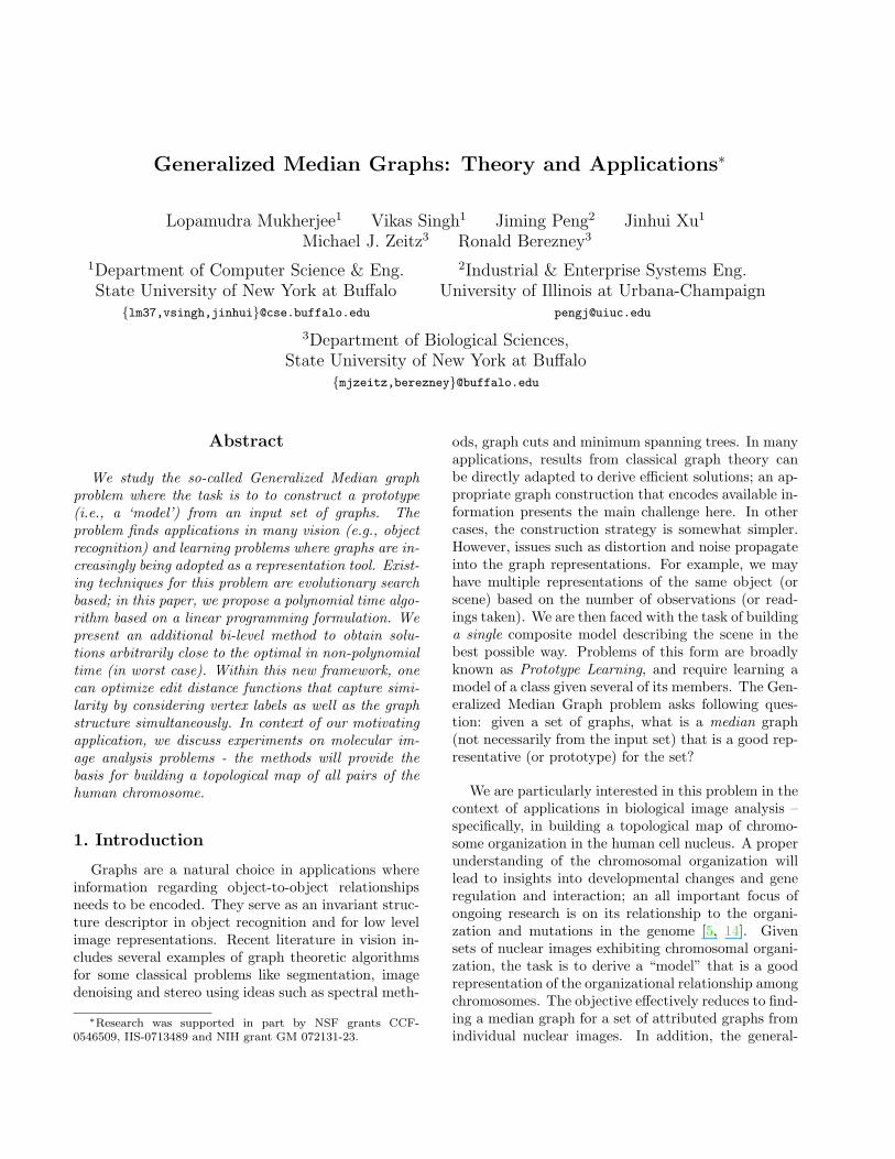
The algorithm in [2] cannot be directly applied tothe isomorphism problem on general graphs with un-equal number of vertices or vertex labeled graphs. Themore general case of vertex labeled graphs with weightededges adds a new realm of complexity to the problem.To see this, let us consider the factors contributing tothe edit cost in general graphs. Normally, ‘edits’ areperformed on nodes and edges and can be broadly clas-sified as insertion and deletion of nodes (fv(u)), edges(fe(e)) and substitution of nodes (dv(fv(u1), fv(u2)))and edges (de(fe(e1), fe(e2))). The problem of gener-alized graph isomorphism becomes rather ill-posed forthe case where the costs (for nodes and edges) are notdefined in the same metric space. To motivate this ar-gument, let us consider an illustrative example. In Fig.1, we seek to match graphs G0 and G1 in a minimal editcost sense. Assuming vertex substitution has unit cost(Hamming distance) and edge replacement costs are inL1 or L2 space, the matching will favor mapping 4abc

in G0 to 4def in G1 instead of 4abc. Clearly, thematching is a trade-off between competing influences.

Figure 1: Matching with labels and weighted edges.

For the special case of graphs with labeled verticesand unweighted edges, Justice and Hero [11] very re-cently proposed a modification of the algorithm in [2]to define the Graph Edit Distance in terms of an In-teger Linear Programming formulation. This tech-nique allows G0 and G1 to have unequal number oflabeled vertices as follows. An edit grid is constructed,given as a complete graph, GΩ = (VΩ, EΩ) where|VΩ| = N ≤ |V1| + |V2|. The vertex labels belong toan alphabet, Σ. First, the nodes (and edges) on theedit grid are initialized to φ (and 0). Then, the initialgraph G0 is placed on this edit grid. The φ-labeledvertices of the edit grid take the labels of the verticesof G0 that are aligned with them. All edges in GΩ (la-beled 0) are converted to 1 if they denote a real edgein G0. An edit operation on this standard placementof G0 is then defined as either changing the label ofa vertex from a character in Σ to φ denoting deletionor from φ to a character in Σ denoting insertion. Thisamounts to permuting the standard placement of G0

to minimize the following.

min

NXi=1

NXj=1

d(fv(Ai0), fv(Aj

1))Pij +

1

2‖A0 − PA1P

T ‖, (3)

where A0 and A1 are the adjacency matrices of thestandard placements of G0 and G1 on the edit gridand Ai

0 (and Aj1) is the ith (and jth) vertex of A0 (and

A1) and d ∈ 0, 1 is the cost function for the vertices.While vertex and edge edit costs are in the same

space (binary), (3) does not adequately capture thenotion of similarity distance. To see this, consider twoto-be-matched input graphs with vertices having largedegree (≥ 3). If vertices with mismatched labels fromthe two graphs are aligned, one naturally pays a costof 1 for a single vertex pair mismatch. This is clearlysmall compared to the cost incurred when vertices hav-ing a large difference in degree are matched to eachother (see (3)). A natural tendency of the algorithm,therefore, would be to match vertices with the samedegree, instead of vertices with the same label. In fact,one may construct examples where such an approachmay ignore labels almost completely in favor of same-degree-vertex alignments, especially if the vertices havehigh degree. While it could be argued that this is in ac-

cordance with the edit cost definitions, but in most ap-plications, the semantic meaning of a vertex in a graphis as important as its structural relationship with othernodes. For example, in matching graphs that representchemical compounds (e.g., Lewis structure), should wematch a ‘C’ (carbon) to a ‘H’ (hydrogen) simply be-cause they share bonds with the same number (degree)of atoms?

The analysis above indicates that using edit distanceas a cost function in many applications yields a bi-ased weighted matching where a degree mismatch has ahigher penalty. Therefore, we must somehow re-weightthe cost of replacing vertices to reflect the vertex labelsas well as the associated edge information (structure)concurrently. We will discuss these issues next.

2. Main Ideas

2.1. A suitable cost function

Consider an image registration problem where theimages have colored regions or certain segmented ob-jects. The image’s graph representation would natu-rally encode the regions as vertices with the respectivecolors as their labels. Additionally, edges between thevertices may denote some ‘link’ between their corre-sponding regions or relationships between objects asobserved in the image. The registration problem thenrequires one to match the images (or its correspondinggraph link structures) in a manner that matches similarcolors (regions) while maximally preserving the graphtopologies. By this interpretation, there is a cost asso-ciated with the extent of similarity of two colors. Forexample, matching a blue vertex with a green vertex hasa higher cost compared to matching a blue vertex witha cyan vertex. This cost is different from edge weights;while label-to-label cost relates vertices in source andtarget graphs, edge weights usually denote the strengthof a ‘relation’ between vertices in the same graph.

To address the ill-posedness problem outlined in §1.2while preserving the intuitions discussed above, we con-sider a generalization of edit distances for matchinggraphs. We will focus on matching edges alone; for-tunately, since edges are identified by their end ver-tices, it is possible to align vertices implicitly whilealigning edges explicitly as we illustrate now. Assumewe are given two to-be-matched vertex labeled graphs,G0 = (V0, E0, fv, fe) and G1 = (V1, E1, fv, fe). Weare also given a matrix, S , indicating similarity be-tween vertex labels. The entry, S (i, j) indicates theextent of dissimilarity between labels (colors) i and j;S (i, j) = 0 if i = j. The presence or absence of a linkbetween vertices is indicated by their edge weights, fe

where fe ∈ 0, 1. An explicit match between edgeei = (a, b) ∈ G0 and ej = (c, d) ∈ G1 aligns the twovertices of the edges i.e., a→ c, b→ d. Therefore, while

we do not focus on matching vertices, we can indirectly‘charge’ vertices with misaligned labels. This idea al-lows us to naturally derive the cost that must be paidwhen an edge ei = (a, b) (in source) is matched withanother edge ej = (c, d) (in target) given as

cost(ei, ej) = S (a, c) + S (b, d) + ‖fe(ei)− fe(ej)‖, (4)

where the cost(ei, ej) = 0 if both end vertices of theedge pair match perfectly. Otherwise, it reflects sumof the costs of (i) misaligned vertices (based on thedissimilarity of aligned vertex labels) and (ii) differenceof weights of the edges (which is 0 unless it is matchedto a null edge).

While (4) allows evaluating the cost due to ver-tex mismatches given two aligned edges as parame-ters, we must represent the sum of such costs for apair of graphs in an algebraically computable man-ner – to define what must be optimized. Suppose avertex u1 ∈ G0 is aligned with u2 ∈ G1 such thatS (u1, u2) > 0. Each edge incident on u1 pays a cost ofS (u1, u2) due to a misaligned u1. Thus, the total costis deg(u1) ·S (u1, u2) where deg(·) denotes the degreeof a vertex. Similarly, the cost for all incident edges ofu2 is deg(u2) ·S (u1, u2). The total cost of one vertexmisalignment pair (u1 ↔ u2) is then

D(u1, u2) = [deg(u1) + deg(u2)] ·S (u1, u2). (5)

Notice that all edges associated with u1 and u2 havepaid only part of their cost (due to vertex misalign-ment on one side and reflecting the first term in (4)).However, the second vertex of edge ei (see second termin (4)) is automatically considered at the time of eval-uation of the other pair of aligned vertices. The costfunction that models this is

min

NXi=1

NXj=1

D(i, j)P ij +1

2‖A0 − PA1P

T ‖. (6)

The second term in (6) evaluates the cost of matchinga ‘real’ edge to a ‘non-existent’ or null edge (see thirdterm in (4)). But, (6) as a measure of graph similar-ity is still not entirely accurate. It is perfect when anedge matches with a null edge; however, when an edgematches to another real edge, the cost due to S (u1, u2)is counted twice (for u1 ∈ G0 and for u2 ∈ G1). Thisoverestimation must be deducted to reflect the actualcost. We will discuss this shortly.

For convenience of presentation, let us first general-ize the notion of graph similarity distance (in (6)) inthe context of median graphs. Addressing the overesti-mation issues discussed above in the generalized setupturns out to be significantly easier. Notice that whenwe have just two graphs, the cost calculated is the simi-larity of one graph to the permuted version of the other.In our formulation, all the input graphs are embedded

(placed) in an edit grid, GΩ, |GΩ| ≥ N . Here, a per-mutation is simply a change of placement from oneposition to the other. Hence, the generalized median isa graph on the edit grid that minimizes the distance ofevery graph in the input set (post-permutation) to it-self. This distance is clearly zero when all input graphsare isomorphic. Extending this logic to the general casewhere input graphs are not necessarily isomorphic, ourobjective is to find a set of permutations – one for eachgraph such that the resultant set of placements are thesame (or as close as possible). It can be verified that themean of all such close placements will yield the general-ized median for the set of input graphs. Because whichpermutation must be applied to a certain graph is notknown in advance, we must simultaneously permuteall pairs of graphs, and calculate the cost incurred. Inthe next section, we will introduce the integer programthat models this intuition. We will then address theoverestimation in (6). Throughout this paper, uppercase letters (A) and upper case letters with a singlesubscript (A0) will denote matrices; upper case letterswith two subscripts or two superscripts will refer toindividual matrix entries (Aij , Aij

0 , and A(i, j)).

2.2. Cost when both graphs are permuted

The edit grid, GΩ, provides a common ‘reference’frame in which the the sum of variations (cost) betweenthe permuted graphs can be defined and computed pre-cisely. Let us first consider the cost definition when twographs are simultaneously permuted onto GΩ and thenextend the definition for multiple graphs. If graphs, G0

and G1, are permuted by P0 and P1 respectively, (6) isrepresented as follows.

NXi=1

NXk=1

NXj=1

D(i, j)P ik0 P kj

1 +1

2‖P0A0P

T0 − P T

1 A1P1‖, (7)

where P ik0 = 1 indicates that vi ∈ G0 is permuted

to position k on the edit grid. A triplet, (i, j, k), suchthat P ik

0 P kj1 = 1 implies that vi ∈ G0 is permuted to

the position k, and position k on the edit grid mapsto vj ∈ G1 and so we must incur a cost, D(i, j). Themain difficulty in (7) involves the product term of twovariable matrices, P0 and P1. Our linearization in-volves an additional variable X ∈ <N×N×N , Xijk is1 if P ik

0 P kj1 = 1 and 0 otherwise. This naturally yields

P ik0 + P kj

1 = 2 =⇒ Xijk = 1. (8)

(8) can be converted to regular linear constraints as

P ik0 + P kj

1 ≥ 2Xijk,

P ik0 + P kj

1 − 1 ≤ Xijk. (9)

Observe that when P ik0 + P kj

1 = 2, Xijk must be1 to simultaneously satisfy both constraints in (9); if

P ik0 + P jk

1 ≤ 1, Xijk must be 0. (8) and (9) are henceequivalent. Incorporating these into (7) gives

NXi=1

NXj=1

D(i, j)(

NXk=1

Xijk) +1

2‖P0A0P

T0 − P T

1 A1P1‖. (10)

We now revisit the overestimation issues from §2.1.To calculate the overestimation in (10), we first needto determine the edge-to-edge mappings between G0

and G1. This is given by the “1” entries in the dotproduct of P0A0P

T0 and PT

1 A1P1. The overestimation,say C ∈ <n×n, is associated with (i, j) positions with1s and must be deducted. For presentation purposes,let us define the following notations

γ = (P0A0PT0 + P T

1 A1P1), γ = (P0A0PT0 − P T

1 A1P1), (11)

φ(S , X)i =

NXi1=1

NXj1=1

S (i1, j1)Xi1j1i, (12)

Then,

Cij =

(φ(S , X)i + φ(S , X)j if γij = 2;

0 if γij ≤ 1

(13)

Notice that for an edge, eij , when the sum in (13) is 2,i.e., when the the dot product of P0A0P

T0 and PT

1 A1P1

at position (i, j) is 1, Cij is non-zero (i.e., equal to theovercharged cost of matching the end vertices of eij).Here, i and j denote the indices of vertices of the indi-vidual graphs after permutation, these can be mappedback to the original indices of those vertices in G0 andG1 using X. Let M be the maximum mismatch costof an edge (computed offline, see (4)). The conditionalconstraints in (13) can then be easily expressed as

φ(S , X)i + φ(S , X)j − Cij ≤ (2− γij)M,

C ≤ MP0A0PT0 , C ≤ MP T

1 A1P1. (14)

Here, the constraints (denoted without subscripts) ap-ply for all matrix elements. Therefore, the final objec-tive function that takes care of the overestimation is

min

NXi=1

NXj=1

D(i, j)(

NXk=1

Xijk)+1

2‖γ‖− 1

2

NXi=1

NXj=1

Cij| z overestimation

, (15)

where γ is as defined in (11) and the constraints are

P0e = e; P T0 e = e; P1e = e; P T

1 e = e, (16)

P ik0 + P kj

1 ≥ 2Xijk, P ik0 + P kj

1 − 1 ≤ Xijk, (17)

φ(S , X)i + φ(S , X)j − Cij ≤ (2− γij)M, (18)

C ≤ MP0A0PT0 , C ≤ MP T

1 A1P1, (19)

P0, P1, X ∈ 0, 1; C ∈ [0, M ]. (20)

Remark: When only one graph is permuted, the sim-pler model only has O(n2) variables and constraints.

3. Linearization and Relaxation

In this section, we describe a relaxation technique toderive a polynomial time solvable version of the prob-lem in §2.2. We illustrate the ideas using the familiarobjective function in (2) in §1.2. The strategy appliesreadily to (15)-(20). We observe that the objective,∑

ij(AG1 − PAG2PT )ij , is equivalent toX

l

(vec(AG1)− vec(AG2)(P ⊗ P ))l, (21)

where ⊗ indicates the Kronecker product and vec(·)vectorizes a matrix by stacking its columns. Considera matrix variable Q where Q = P ⊗P , the nonlinearityin the second term can be addressed as follows.X

l

(vec(AG1)− vec(AG2)Q)l, (22)

where Q ∈ Πn2 and Πd denotes permutation matri-ces of size d× d. Note that the relaxation in [2] worksperfectly when only one graph is permuted, (2) is usedonly as an example. Q has some additional interestingproperties; specifically, the (i, j)th block of Q, denotedas Q[ij] corresponds to element P ij . Below, Q(i, j) de-notes the (i, j)th entry of Q and S, T are slack variables.The resultant LP is

minX

(S + T ) (23)

s.t. vec(AG1)− vec(AG2)Q + S − T = 0nX

l=1

Q(k + (i− 1)n, (j − 1)n + l) = P ij ,∀i, j, k

nXi=1

Q[ij] = P,

nXj=1

Q[ij] = P, ∀i, j ∈ [1, n],

P e = e; eT P = eT ; P, Q, S, T ≥ 0. (24)

The relaxation of (23)-(24)is polynomial time solvable.

4. Generalized Median Graphs

A natural extension of (15)-(20) yields a model forcomputing the generalized median graph for a set. Letthe ‘distance’ between two graphs as defined in (15)be given as dp(G0, G1, P0, P1). Notice that while dp(·)simply computes the cost given four parameters (nounknowns), (15) tries to optimize the distance wherethe permutations are unknown. Using the notationabove, our objective is to permute all graphs onto theedit grid and can be expressed as

min

KXx=1

KXy=1

dp(Gx, Gy, Px, Py), (25)

where K is the number of graphs in the set. The 0-1 solution can be obtained by rounding the fractionalentries of the K permutation matrices and obtainingthe median graph as a mean of the permuted input

graphs. This yields a polynomial time algorithm forcomputing the generalized median graph, no boundedrunning time algorithms were known before.

Our experimental results using this model are dis-cussed in §5. In general, this approach can be usedfor reasonably sized graphs (no assumptions on thestructure) and yields good results in practice. Sincethe number of variables in the model are O(N4K), forlarge graphs some application specific heuristics mayneed to be employed. In the following sections, em-ploying the ideas above we discuss a hybrid approachthat yields a factor two approximation ratio if graphdistances are known correctly. Finally, we propose an-other bi-level algorithm that finds a solution arbitrar-ily close to the optimal (though running time is non-polynomial in worst case).

We employ the concept of generalized median for aset of objects in metric spaces [9] as a first step. Let thedistance (discussed above) between two graphs be givenas d(G0, G1) = dp(G0, G1, I, P1). We first introducethe following result.

Lemma 1 For any three graphs Gp, Gq and Gr,d(Gp, Gq) ≤ d(Gp, Gr)+d(Gq, Gr) i.e., d(·, ·) is metric.

Let G = (G0, G1, . . . , GK) be a collection of graphswith |Vi| = |Vj |,∀i, j. Dummy nodes can be introducedif |Vi| 6= |Vj |, so N = max(|V1|, . . . , |Vn|). Let G∗ be theoptimal median of this set. By definition, G∗ satisfies

G∗ = arg minG

KXi=1

d(G, Gi)

We will avoid computing G∗ directly. Instead, weemploy the lower bounding ideas in [9] to model thedistance of every graph, Gi to the generalized medianby an unknown variable, xi. Therefore, xi = d(G∗, Gi).Then, the problem can be modeled as follows.

min

KXi=1

xk (26)

s.t. xk + d(Gk, Gl) ≥ xl,∀k, l,

xl + d(Gk, Gl) ≥ xk,∀k, l,

xk + xl ≥ d(Gk, Gl),∀k, l,

xi ≥ 0,∀i ∈ [1, K]. (27)

(26)-(27) can be solved optimally in polynomial time.

Property 1 (from [9]) The sum of the entries of x =(x1, . . . , xK)T denotes a lower bound on the distance ofall graphs to the optimal generalized median.

Lemma 2 There must be a graph Ga ∈ G that satisfies

KXi=1

d(Gk, Ga) ≤ 2

KXi=1

d(Gk, G∗),

where G∗ is the optimal median graph for G.

Proof: Let x∗ = (x∗1, . . . , x∗K)T be an optimal so-

lution for (26)-(27). Consider a graph Ga ∈ G s.t.a = j : x∗j ≤ x∗i ,∀i ∈ [1,K]. From (27), we know∀Gi, d(Gi, Ga) ≤ x∗i + x∗a. Since xa ≤ x∗i , d(Gi, Ga) ≤2x∗i . Therefore

∑Ki=1 d(Gi, Ga) ≤ 2

∑Ki=1 x∗i . Applying

Property 1, the lemma follows.

Theorem 1 The graph Ga ∈ G, a = j : x∗j ≤x∗i ,∀i ∈ [1,K], is a 2-approximation for the gener-alized median graph problem if d(·, ·) is known.

If d(·, ·) is known correctly, the factor two approxi-mation (for the Hybrid algorithm) holds by comparingthe solutions of (26)-(27) and (15)-(20) and outputtingthe better solution.

4.1. Alternate bi-level algorithm (A sketch)

Let U =∑K

i=1 d(Gk, Ga). We know that the op-timal solution lies in [

∑i x∗i , U ]. We adopt a binary

search in [∑

i x∗i , U ] starting at a value c =∑

i x∗i andsolving a feasibility problem (FP) at each step. Theobjective function of the FP is max 0 subject to theconstraints that the sum of distances of Gi ∈ G toan unknown graph G is upper bounded by c. Herethe adjacency matrices of G and Pi are variables. Theconstraints are defined by (15)-(20). If this returns afeasible solution, we are done (i.e., G = G∗). Other-wise, we continue the binary search. The FP can besolved using branch-and-bound type methods (avail-able in most commercial solvers like CPLEX) but mayhave non-polynomial running time in the worst case.

5. Experimental Results

We discuss experiments related to our motivating bi-ological image analysis application. Results on patternrecognition graph database and applications in drug-design will appear in the longer version of the paper.

5.1. Applications in Biological Image Analysis5.1.1 Brief Biological background

Chromosomes within the human cell nucleus are knownto occupy discrete territories and evidence from recentliterature suggests that these might be functionally rel-evant because the position of these territories in nuclearspace is ‘organized’ [5]. It shows a statistical correla-tion with gene density and the size of chromosomes[7]. In humans, larger chromosomes (numbers 1 − 10)are arranged on the periphery. Secondly, chromosomesmay have non-random neighbors, a finding that mightaccount for preferential translocations and interactionsbetween specific chromosomes. Biologists suspect thatsuch patterns are related to genomic evolution and cell-type-specific variability.

Figure 2: A nuclear im-age with eight chromosomepaints.

In this regard, severalresearchers[3, 13] havestressed on the need ofmapping large-scale orga-nization and distributionof chromatin in variouscell lines. The standardapproach relies on asequence of experimentson a large number ofcells. Chromosome tochromosome relationshipsare manually investigatedusing the acquired images(see Fig. 2, one for every cell) sequentially. A reliabletopological ‘model’ can provide the necessary founda-tion for studying the effect of higher-order chromatindistribution on nuclear functions. Unfortunately, anarrangement map for all 23 chromosome pairs in adiploid human cell nucleus is lacking so far. Suchmodels are needed for different cell types at variousstages of cell cycle and terminal differentiation [3].5.1.2 Chromosomal organization maps

Topological map derivation of chromosomes transformsnaturally to the generalized median graph problem.Each individual chromosome (denoted as numbers inFig. 2) is represented as a labeled vertex in a graph.Due to microscopic acquisition limitations, at most 8pairs of chromosomes can be ‘labeled’ per cell; hence,our graph has 16 vertices with at most 2 verticeswith the same vertex label (i.e., chromosome number-ing). Spatial proximity (adjacency) between chromo-somes is expressed as an edge between vertices. Wefocus on 8 pairs of the larger chromosomes (numbers1, 2, 3, 4, 6, 7, 8, 9) from the human lung fibroblast cellline. The acquisition process was repeated for 37 cellsoverall. The raw images were segmented to createmasks for individual chromosome pairs and individualgraph representations derived (see Fig. 3).

To evaluate the goodness of our final ‘model’, we di-vide the cells into a training set (19 cells) and a testset (18 cells). We report on the following observations.Optimality. Figure 3 (g) shows the median graph ob-tained from the training set. The objective functionvalue was 1.43 times the lowest possible cost for com-puting the median for this set of graphs (lower boundby (26)-(27)). This ratio for the training, test, en-tire set medians were 1.58,1.6,1.63 indicating thatthe computed generalized median is a better represen-tative for the set than any of the component graphs.Note: Exhaustive enumeration analysis suggests thata solution much closer to the lower bound is unlikely.Substructure frequency. We generated groups of

chromosomes which occur frequently as a chain or asub-group (e.g., numbers (b, c, d)) by graph mining [1]and other software [12]. We then compared these tothe results obtained by the median graph model forthis cell line. Figure 3(h) shows groups (colored edges)with an occurrence frequency of ≥ 70%. Fig. 3(h)shows that almost all such sub-graphs align perfectlywith the computed median graph indicating that themodel incorporates the essential information from theconstituent graphs. Notice that while the median canfit all subgraphs, all subgraphs cannot build the model.Structure Prediction. The basic question we wantedto answer was – given a new cell, can we predict thenon-random part of its chromosomal organization? Ifyes, then the model serves its purpose and can be usedto interpret biologically relevant information. To dothis we calculated Jaccard’s, Sorensen’s, and Mount-ford’s similarity of the median (from training set) witheach cell in the training/test set (considering attributededges as set members). The results in Fig. 3(i) showthat the similarity is only slightly worse for the test setw.r.t. the training set. Considering that Sorensen’s is apercentage similarity measure, we can draw the follow-ing inference – given a new cell, we can predict closeto 50% of its chromosome organization. This means∼ 50% of chromosomal relationships are preserved!

6. Conclusions

This paper applies mathematical programming todesign an optimization framework for the generalizedmedian graph problem in context of a real world vi-sion problems in biological image analysis. In addition,the concept has applications to drug-design (structuralpattern recognition) and other problems, we believethat the ideas will find general applicability in build-ing exemplars from representations such as attributedskeletal graphs. The extension of the similarity metricis also of independent interest.

References

[1] IBM Frequent Subgraph Miner(http://www.alphaworks.ibm.com/tech/fsm). 7

[2] H. A. Almohamad and S. O. Duffuaa. A linear pro-gramming approach for the weighted graph matchingproblem. IEEE PAMI, 15(5):522–525, 1993. 2, 3, 5

[3] S. Boyle, S. Gilchrist, J. Bridger, N. L. Mahy, J. A.Ellis, and W. A. Bickmore. The spatial organizationof human chromosomes within the nuclei of normal andemerin-mutant cells. Hum. Mol. Genet., 10:211–219,2001. 7

[4] D. G. Corneil and C. C. Gotlieb. An efficient algorithmfor graph isomorphism. J. ACM, 17(1):51–64, 1970. 2

[5] T. Cremer and C. Cremer. Chromosome territories,nuclear architecture and gene regulation in mamaliancells. Nature Reviews Genetics, 2:292–301, 2001. 1, 6

(a) (b) (c)

(d) (e) (f)

(g) (h) (i)Figure 3: 2D sections of chromosome organization in 3 cell-images in (a)-(c) and their graphical representation in (d)-(f);a generalized median graph for a set of 19 cells in (g); all patterns (except one) with frequency of ≥ 70% across 19 cells (bygraph-mining) were present in the generalized median graph and shown as colored in (h); average of similarity measures ofitems in the test/training sets w.r.t. to the generalized median and set median of those sets in (i).

[6] P. W. Finn, S. Muggleton, D. Page, and A. Srini-vasan. Pharmacophore discovery using the inductivelogic programming system PROGOL. Machine Learn-ing, 30(2-3):241–270, 1998. 2

[7] H. Tanabe et al. Evolutionary conservation of chromo-some territory arrangements in cell nuclei from higherprimates. PNAS, 99(7):4424–4429, 2002. 6

[8] A. Hlaoui and S. Wang. Median graph computationfor graph clustering. Soft Comp., 10(1):47–53, 2006.2

[9] X. Jiang and H. Bunke. Optimal lower bound for gen-eralized median problems in metric space. In Proc.IAPR SSSPR, pages 143–152, 2002. 6

[10] X. Jiang, A. Munger, and H. Bunke. On me-dian graphs: Properties, algorithms, and applications.IEEE PAMI, 23(10):1144–1151, 2001. 2

[11] D. Justice and A. Hero. A binary linear programmingformulation of the graph edit distance. IEEE PAMI,28(8):1200–1214, 2006. 3

[12] L. Mukherjee, V. Singh, J. Xu, K. Malyavantham, andR. Berezney. On mobility analysis of functional sites

from time lapse microscopic image sequences of livingcell nucleus. In MICCAI, pages 577–585, 2006. 7

[13] R. Nagele, T. Freeman, L. McMorrow, and H. Lee.Precise spatial positioning of chromosomes duringprometaphase: Evidence for chromosomal order. Sci-ence, 270:1830–1835, 1998. 7

[14] L. Parada, P. G. McQueen, P. J. Munson, and T. Mis-teli. Conservation of relative chromosome positioningin normal and cancer cells. Curr. Biol., 12(19):1692–1697, 2002. 1

[15] C. A. Phillips and T. Warnow. The Asymmetric Me-dian Tree: A New Model for Building Consensus Trees.Discrete Appl. Math., 71(1-3):311–335, 1996. 2

[16] S. Toda. Graph Isomorphism: Its Complexity and Al-gorithms. In Proc. FSTTCS, page 341, 1999. 2

[17] J. R. Ullmann. An algorithm for subgraph isomor-phism. J. ACM, 23(1):31–42, 1976. 2

[18] S. Umeyama. An eigendecomposition approach toweighted graph matching problems. IEEE PAMI,10(5):695–703, 1988. 2