Discrete Applied Mathematics 156 (2008) 2719–2739www.elsevier.com/locate/dam

G-graphs: An efficient tool for constructing symmetric andsemisymmetric graphsI

Alain Bretto∗, Luc Gillibert

Universite de Caen GREYC CNRS UMR-6072, Campus 2, Bd Marechal Juin BP 5186, 14032 Caen cedex, France

Received 23 March 2007; received in revised form 7 November 2007; accepted 11 November 2007Available online 22 January 2008

Abstract

Symmetric and semisymmetric graphs are used in many scientific domains, especially parallel computation and interconnectionnetworks. The industry and the research world make a huge usage of such graphs. Constructing symmetric and semisymmetricgraphs is a large and hard problem. In this paper a tool called G-graphs and based on group theory is used. We show the efficiencyof this tool for constructing symmetric and semisymmetric graphs and we exhibit experimental results.c© 2007 Elsevier B.V. All rights reserved.

Keywords: Graph theory; Graphical representation of group; Symmetric graph; Semisymmetric graph

1. Introduction

A graph that is both edge-transitive and vertex-transitive is called a symmetric graph. Such graphs are used in manydomains, for example, the interconnection network of SIMD computers. But constructing them is a problem.

Usually, the graphical representation of groups is used for the construction of those graphs. A popular represen-tation of a group by a graph is the CAYLEY representation. A lot of work has been done about these graphs [1,9].CAYLEY graphs have very nice highly regular properties. But CAYLEY graphs are always vertex-transitive, and thatcan be a limitation. In this article we present and use G-graphs introduced in [18]. Some properties of these graphshave been studied in [2–4]. G-graphs, like CAYLEY graphs, have highly regular properties; consequently G-graphs area good alternative tool for constructing some symmetric graphs. After the definition of these graphs we give a charac-terisation of bipartite G-graphs. Then, using this characterisation, we build a powerful algorithm based on G-graphsfor computing symmetric graphs.

The classification of symmetric graphs is a very interesting problem. Ronald M. FOSTER started collectingexamples of small cubic symmetric graphs prior to 1934, maintaining a census of all such graphs. In 1988 a versionof the census was published in a book containing some graphs up to order 512 [5]. Finally, in 2006, Marston Conderpublished on the Web a list of all the cubic symmetric graphs up to the order 2048 [8]. But symmetric graphs are not

I A short version of this work has been presented to ISSAC’05 [A. Bretto, L. Gillibert, Symmetric and semisymmetric graphs construction usingG-graphs, in: Proceedings of ISSAC’05, July 24–27, 2005, Beijing, China. ACM Proceedings, 2005, pp. 61-67].

∗ Corresponding author. Fax: +33 (0)2 31 56 73 30.E-mail addresses: alain.bretto@info.unicaen.fr (A. Bretto), luc.gillibert@info.unicaen.fr (L. Gillibert).

0166-218X/$ - see front matter c© 2007 Elsevier B.V. All rights reserved.doi:10.1016/j.dam.2007.11.011

2720 A. Bretto, L. Gillibert / Discrete Applied Mathematics 156 (2008) 2719–2739

the only interesting graphs. There exist regular graphs which are edge-transitive but not vertex-transitive [11,15,16];they are called semisymmetric graphs, and it is quite difficult to construct them [12,10,17]. In this paper we exhibit anefficient algorithm, based on G-graphs, for constructing cubic semisymmetric graphs. So, with G-graphs, it becomeseasy not only to reconstruct the The Foster Census up to order 1320 but also to construct cubic semisymmetric graphs,quartic symmetric and semisymmetric graphs, quintic symmetric and semisymmetric graphs and so on.

2. Basic definitions

2.1. Graph definitions

We define a graph Γ = (V ; E; ε) as follows:

• V is the set of vertices and E is the set of edges.• ε is a map from E to P2(V ), where P2(V ) is the set of subsets of V having 1 or 2 elements.

In this paper graphs are finite, i.e., sets V and E have finite cardinalities. For each edge a, we define ε(a) = [x; y]

if ε(a) = x, y with x 6= y or ε(a) = x = y. If x = y, a is called loop. The elements x, y are called extremitiesof a, and a is incident to x and y. The set a ∈ E, ε(a) = [x; y] is called multi-edge or p-edge, where p is thecardinality of the set. We define the degree of x by d(x) = card(a ∈ E, x ∈ ε(a)).

Given a graph Γ = (V ; E; ε), a chain is a non-empty graph P = (V, E, ε) with V = x0, x1, . . . , xk andE = a1, a2, . . . , ak−1ak, where xi , xi+1 (i mod k) are extremities of ai . The elements of E must be distinct. Thecardinality of E is the length of this chain. A graph is connected if, for all x, y ∈ V , there exists a chain from x to y.

Γ ′= (V ′

; E ′; ε′) is a subgraph of Γ if it is a graph satisfying V ′

⊆ V , E ′⊆ E and ε′ is the restriction from ε to

E ′. If V ′= V then Γ ′ is a spanning subgraph.

An induced subgraph is generated by A, Γ (A) = (A; U ; ε), with A ⊆ V , and U ⊆ E a subgraph such asU = a ∈ E, ε(a) = [x; y], x, y ∈ A.

An induced subgraph such that any pair of vertices are adjacent is called a clique. Let Γ = (V ; E; ε) be a graph; acomponent of Γ is a maximal connected induced subgraph.

Let Γ1 = (V1; E1; ε1) and Γ2 = (V2; E2; ε2) be two graphs; a morphism from Γ1 = (V1; E1; ε1) to Γ2 =

(V2; E2; ε2) is a couple ( f, f #) where f : V1 −→ V2 is a map and f #: E1 −→ E2 is a map such that

if ε1(a) = [x; y] then ε2( f #(a)) = [ f (x); f (y)].

So (idV , idE ) is a morphism from G = (V ; E; ε) to G.The product of two morphisms ( f, f #) and (g, g#) is defined by: ( f, f #) (g, g#) := ( f g, f #

g#). ( f, f #)

is an isomorphism if there exists a morphism (g, g#) from Γ2 = (V2; E2; ε2) to Γ1 = (V1; E1; ε1) such that(g, g#) ( f, f #) = (idV1 , id#

E1) and ( f, f #) (g, g#) = (idV2 , id#

E2). In this case we will define (g, g#) = ( f, f #)−1.

So ( f, f #) is an isomorphism if and only if f is a bijection and f # is a bijection. If there exists an isomorphismbetween Γ1 and Γ2 we will denote this as Γ1 ' Γ2 and we will say that Γ1 is isomorphic to Γ2.

A graph Γ = (V ; E; ε) is k-partite if there is a partition of V into k parts such that any part does not contain anyedge other than loops. We will write Γ = (ti∈I Vi ; E; ε), card(I ) = k. A graph is minimum k-partite, k ≥ 2, if itis not (k − 1)-partite. It is easy to verify that for any graph Γ there exists k such that Γ is minimum k-partite. If agraph Γ is k-partite we will say that (Vi )i∈1,2,...,k is a k-representation of Γ and we will call (Γ , (Vi )i∈1,2,...,k) ak-graph. A minimum k-partite graph is semi-regular if there exists a k-representation (Vi )i∈1,2,...,k such that, for alli ∈ 1, 2, . . . , k, all the vertices of Vi have the same degree.

A k-graphs morphism ( f, f #) is morphism from a k1-graph (Γ1, (V1,i )i∈1,2,...,k1) to a k2-graph(Γ2, (V2, j ) j∈1,2,...,k2) verifying the following property:

For all i ∈ 1, 2, . . . , k1, there exists j ∈ 1, 2, . . . , k2 such that f (V1,i ) ⊆ V2, j .

2.2. Group definitions

In this paper, groups are also finite. We denote the unit element by e. Let G be a group, and let S = s1, s2, . . . , sk,a non-empty set of elements of G. S is a set of generators from G if any element θ ∈ G can be written in the following

A. Bretto, L. Gillibert / Discrete Applied Mathematics 156 (2008) 2719–2739 2721

way: θ = si1 si2 si3 . . . sit with i1, i2, . . . it ∈ 1, 2, . . . , k. We say that G is generated by S = s1, s2, . . . , sk andwe write G = 〈s1, s2, . . . , sk〉. A group G is said to act in the left way on a space Ω when the following operation(a, x) −→ a.x from G × Ω to Ω holds:

• e.x = x .• a.(b.x) = (a.b).x ., a, b ∈ G and x ∈ Ω .

A group action is transitive if it possesses only a single group orbit, i.e., for every pair of elements x and y, there isa group element g such that g.x = y. Let H be a subgroup of G; we write H x instead of Hx. The set H x is calleda right coset of H in G. A subset TH of G is said to be a right transversal for H if H x, x ∈ TH , is precisely the setof all cosets of H in G.

An S-group is a couple (G, S) where G is a finite group and S is a subset of G. A S-groups morphism between(G1, S1) and (G2, S2) is a morphism f from G1 to G2 such that f (S1) ⊆ S2. An automorphism of an S-group is abijective morphism from (G, S) to (G, S). We denote by Aut(G, S) the group of the automorphisms of (G, S).

2.3. Automorphism group

An automorphism of Γ is an isomorphism form Γ to Γ . We denote by Aut(Γ ) the group of the automorphisms ofΓ . We denote by Aut∗(Γ ) the group of the edge-automorphisms of Γ . Both Aut(Γ ) and Aut∗(Γ ) act on Γ . A vertex-transitive graph is a graph whose automorphism group Aut(Γ ) acts transitively on its vertices. An edge-transitivegraph is a graph whose edge-automorphism group Aut∗(Γ ) acts transitively on its edges. A graph that is both edge-transitive and vertex-transitive is called a symmetric graph. A regular graph that is edge-transitive but not vertex-transitive is called a semisymmetric graph.

3. Group to graph process

3.1. Mathematical definition

Let G be a group with a set of generators S = s1, s2, s3, . . . , sk, k ≥ 1. For any s ∈ S, we consider the leftaction of the subgroup H = 〈s〉 on G. So we have a partition G =

⊔x∈Ts

〈s〉x , where Ts is a right transversal of 〈s〉.The cardinality of 〈s〉 is o(s), the order of the element s.

Let us consider the cycles

(s)x = (x, sx, s2x, . . . , so(s)−1x)

of the permutation gs : x 7−→ sx of ΣG . Hence 〈s〉x is the support of the cycle (s)x . Notice that just one cycle of gscontains the unit element e, namely (s)e = (e, s, s2, . . . , so(s)−1). We define a graph denoted by Φ(G; S) = (V ; E; ε)

in the following way:

• The vertices of Φ(G; S) are the cycles of gs , s ∈ S, i.e., V = ts∈S Vs with Vs = (s)x, x ∈ Ts.• For each (s)x, (t)y ∈ V , if card(〈s〉x ∩ 〈t〉y) = p, p ≥ 1 then 〈s〉x, 〈t〉y is a p-edge.

Thus, Φ(G; S) is a k-partite graph and any vertex has a o(s)-loop. We denote as Φ(G; S) the graph Φ(G; S)without loops. By construction, one edge stands for one element of G. We can remark that one element of G can labelseveral edges. Both graphs Φ(G; S) and Φ(G; S) are called graphs from groups or G-graphs and we can say that thegraph is generated by the group (G; S). If S = G, the G-graph is called the canonic graph.

3.2. Algorithmic procedure

The following procedure constructs a graph from a group G and a subset S of G. A list of vertices and a list ofedges represent the graph:

2722 A. Bretto, L. Gillibert / Discrete Applied Mathematics 156 (2008) 2719–2739

Procedure Group To Graph(G, S)Data:

G a groupS = s1, s2, s3, . . . , sk, a subset of G

Cycles computingL = ∅

for all a in Sl2 = ∅

gs = ∅

for all x in Gif x not in l2 then

l1 = ∅

for k = 0 to k = Order(a)− 1Add (ak)× x to l1Add (ak)× x to l2

end forAdd l1 to gs

end ifend forAdd gs to L

end forGraph computing

for all s in LAdd s to Vfor all s′ in L

for all x in sfor all y in s′

if x = y thenAdd (s, s′) to E

end ifend for

end forend for

end forReturn (V, E)

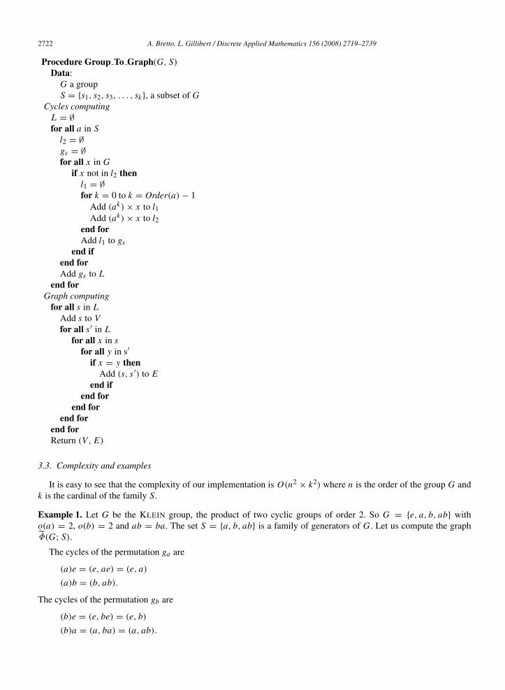
3.3. Complexity and examples

It is easy to see that the complexity of our implementation is O(n2× k2) where n is the order of the group G and

k is the cardinal of the family S.

Example 1. Let G be the KLEIN group, the product of two cyclic groups of order 2. So G = e, a, b, ab witho(a) = 2, o(b) = 2 and ab = ba. The set S = a, b, ab is a family of generators of G. Let us compute the graphΦ(G; S).

The cycles of the permutation ga are

(a)e = (e, ae) = (e, a)

(a)b = (b, ab).

The cycles of the permutation gb are

(b)e = (e, be) = (e, b)

(b)a = (a, ba) = (a, ab).

A. Bretto, L. Gillibert / Discrete Applied Mathematics 156 (2008) 2719–2739 2723

Fig. 1. The octahedral graph.

Fig. 2. The G-graph associated with K2,3.

The cycles of the permutation gab are

(ab)e = (e, abe) = (e, ab)

(ab)a = (a, aba) = (a, b).

The graph Φ(G; S) is isomorphic to the octahedral graph (see Fig. 1). The octahedral graph is a 3-partite symmetricquartic graph.

Example 2. Let G be the cyclic group of order 6, G = e, a, a2, a3, a4, a5; it is known that G can be generated by

an element of order 3 and an element of order 2. Let S be a2, a3, (a2)3 = (a3)2 = e. The cycles of the permutation

ga2 are:

(a2)e = (e, a2e, a4e) = (e, a2, a4)

(a2)a = (a, a2a, a4a) = (a, a3, a5).

The cycles of ga3 are

(a3)e = (e, a3)

(a3)a = (a, a3a) = (a, a4)

(a3)a2= (a2, a3a2) = (a2, a5).

The graph Φ(G; S) is isomorphic to K2,3 (see Fig. 2).

4. Properties of the G-graphs

The following two results can be found in [2].

Proposition 1. Let Φ(G; S) = (V ; E; ε) be a G-graph. This graph is connected if and only if S is a generator set ofG.

Proposition 2. Let h be a morphism between (G1, S1) and (G2, S2); then there exists a morphism, Φ(h), betweenΦ(G1; S1) and Φ(G2; S2).

We also have:

Proposition 3. Let Γ be a connected bipartite and regular G-graph of degree p, p being a prime number; then eitherΓ is simple or Γ is of order 2.

2724 A. Bretto, L. Gillibert / Discrete Applied Mathematics 156 (2008) 2719–2739

Fig. 3. The graphs G1 and G2.

Fig. 4. The graphs Gi , i ∈ 3, 4, 5.

Proof. The graph Γ is bipartite and regular of degree p, so Γ = Φ(G, s1, s2) with s1 and s2 two different elementsof order p. But Γ is a connected graph, so the family s1, s2 generates the group G; in other words G = 〈s1, s2〉. Wecan notice that the groups 〈s1〉 and 〈s2〉 are isomorphic to the cyclic group of order p called C p. If 〈s1〉 and 〈s2〉 arenot different we have

〈s1〉 = 〈s2〉 = 〈s1, s2〉 = G.

Therefore Γ is the graph of the cyclic group C p generated by a family S, with S containing two elements of order p,so the order of the graph Γ is 1. Now let us consider the case where 〈s1〉 and 〈s2〉 are different. This is equivalent tosaying that for all t ∈ 1, 2, . . . , p − 1, for all k ∈ 1, 2, . . . , p − 1 we have

st1 6= sk

2 ,

because if st1 = sk

2 , p being a prime number, sk2 is generator of 〈s1〉, and the following equality becomes true:

〈st1〉 = 〈s1〉 = 〈sk

2 〉 = 〈s2〉 = 〈s1, s2〉 = G.

Consequently the only edge between (s1)e and (s2)e is the edge corresponding to e. More generally, let (s1)x and(s2)y be two cycles. If x = y, let us suppose that there exist t ∈ 1, 2, . . . , p − 1, and k ∈ 1, 2, . . . , p − 1 such thatst

1x = sk2 y. We have st

1 = sk2 , and that led us to the first case. So there can be only one edge between (s1)x and (s2)y:

the edge corresponding to the element x . Let us consider the case where x and y are different. If there is a multi-edgebetween (s1)x and (s2)y, then st

1x = sk2 y and sl

1x = si2 y. We can suppose that l = t + n and i = k + m. So we have

the following two equalities:

sl1x = st+n

1 x = sn1 (s

t1x)

sl1x = si

2 y = sk+m2 y = sm

2 (sk2 y).

So sn1 (s

t1x) = sm

2 (sk2 y), but st

1x = sk2 y; consequently sn

1 = sm2 , and that led us to the first case.

We will use this well-known result:

Theorem 1 ([11]). Let Γ be a simple graph. Then Aut1(Γ ) ' Aut∗(Γ ) if and only if:

(a) G1 and G2 are not both components of Γ (see Fig. 3).(b) And none of the graphs Gi , i ∈ 3, 4, 5, is a component of Γ (see Fig. 4).

We are now in position to characterise the bipartite G-graphs:

Theorem 2. Let Γ = (V1, V2; E) be a bipartite connected semi-regular simple graph. Let (G, s1, s2) be an S-groupwith o(s1) = deg(x), x ∈ V1 and o(s2) = deg(y), y ∈ V2. The three following properties are equivalent:

A. Bretto, L. Gillibert / Discrete Applied Mathematics 156 (2008) 2719–2739 2725

(i) The graph Γ = (V1, V2; E) is a G-graph, Φ(G; s1, s2).(ii) The line-graph L(Γ ) is a Cayley graph Cay(H ; A) (where A = 〈a1〉 ∪ 〈a2〉 \ e) with (G, s1, s2) '

(H, a1, a2).(iii) The group G is a subgroup of Aut∗(Γ ) which acts regularly on the set of edges E.

Proof. Suppose that Γ is a G-graph Φ(G; s1, s2). We show that (iii) is true. An edge stands for a unique element ofG and an element of G stands for a unique edge. So it is sufficient to show that the action (left multiplication) of Gon itself preserves the graph Φ(G; s1, s2). Let e1 and e2 be two adjacent edges of Φ(G; s1, s2) and let g−1

∈ G.The images of e1 and e2 are e1.g−1 and e2.g−1. Because e1 and e2 are adjacent we have e1 = sk .u and e2 = sl .u.Hence, e1.g−1

= sk .u.g−1= sk .v and e2.g−1

= sl .u.g−1= sl .v. Consequently, e1.g−1 and e2.g−1 are adjacent and

g induces an automorphism of Aut∗(Φ(G; s1, s2)).By construction we can remark that, for all x ∈ V1, an edge ex incident to x is adjacent to s1.ex , and for all y ∈ V2,

an edge ey incident to y is adjacent to s2.ey .Assume now that (iii) is true and show that the line-graph of LΓ is a Cayley graph verifying the properties of

(ii). Let L(Γ ) = (L(V ); L(E)) be the line-graph of Γ . It is easy to see that Aut1(Γ ) ' Aut (L(Γ )). Moreover,from Theorem 1, we have Aut1(Γ ) ' Aut∗(Γ ), that leads to Aut∗(Γ ) ' Aut (L(Γ )). Consequently the action ofAut∗(Γ ) on E is equivalent to the action of Aut (L(Γ )) on E . Hence Aut (L(Γ )) contains a subgroup (H, a1, a2)isomorphic to (G, s1, s2) which acts regularly on the set of vertices of L(Γ ) which characterise the fact that L(Γ ) isa Cayley graph. Moreover it is easy to see that

A = a1, a21, . . . , ao(a1)−1

1 , a2, a22, . . . , ao(a2)−1

2 .

Let us suppose that (ii) is true. From L(Γ ) we are going to build Γ . For all u ∈ Ta1 , ai1.u; a j

1 .u ∈ L(E),0 ≤ i < j ≤ o(a1) − 1, and for all v ∈ Ta2 , ak

2 .v; al2.v ∈ L(E), 0 ≤ k < l ≤ o(a2) − 1. We have a bijection from

H = L(V ) on E such that two elements of L(V ) are adjacent if and only if the corresponding edges in Γ are adjacent.Let us define (a1).u = (u, a1.u, a2

1 .u, . . . , ao(a1)−11 .u), for all u ∈ Ta1 , and (a2).v = (v, a2.v, a2

2 .v, . . . , ao(a2)−11 .v),

for all v ∈ Ta2 . Now, let us put an edge between (a1).u and (a2).v if and only if card(〈a1〉.u ∩ 〈a2〉.v) = 1. Byconstruction this graph is a graph which has L(Γ ) as line-graph and it is an H -graph. Moreover it has been shownthat if (G; S) ' (H ; A) then Φ (G; S) ' Φ (H ; A).

5. The construction of symmetric and semisymmetric graphs

5.1. Symmetric or semisymmetric graphs of degree p

Let G be a group of order p×n, with p a prime number, G 6= C p, and S a family such that G = 〈S〉 and S = a, b,with a and b of order p. Then the graph Φ(G; S) is simple, bipartite, edge-transitive and regular of degree p. So thereare two possibilities:

1. Φ(G; S) is vertex-transitive, so it is a symmetric graph;2. Φ(G; S) is not vertex-transitive, so it is a semisymmetric graph.

Therefore G-graphs are a very interesting tool for constructing edge-transitive graphs, especially semisymmetricgraphs. We establish a list of all small groups G of order 3 × n such that G is generated by two elements of order 3.For that we use GAP and the SmallGroups library. This library gives access to all groups of certain small orders. Thegroups are sorted by their orders and they are listed up to isomorphism. For computing the list of the groups generatedby two elements of order 3 we use the following algorithm:

result=[];for all g, group of order n

order3=[];for all x in g

if order(x)=3 thenadd x to order3

end ifend for all

2726 A. Bretto, L. Gillibert / Discrete Applied Mathematics 156 (2008) 2719–2739

for all x1 in order3for all x2 in order3, x2>x1

if <x1,x2>=g add (g,<x1,x2>) to resultend for all

end for allend for allreturn result;

After the list is established, it is easy to generate all the corresponding G-graphs and to compute their automorphismgroup with Nauty [13]. If there is only one orbit in the vertex automorphism group, then the graph is vertex-transitiveand symmetric. Otherwise, the graph is semisymmetric, with the automorphism group having two orbits, in view of thefact that every semisymmetric graph is bipartite; see [11]. With that algorithm we establish a list of cubic symmetricgraphs up to the order 1320. All the symmetric cubic graphs were already known up to the order 2048 [8], so no newgraphs are built for this case and the Table 1 contains only the graphs that are G-graphs. The semisymmetric cubicgraphs were only known up to the order 768 [7]. So Table 2 contains some new graphs.

We denote by Sg-o-n the n-th group of order o in the SmallGroups library. The generators are indicated when thegroup is not described in GAP as a subgroup of Sn . The known graphs are named as in [8].

Table 1Cubic symmetric G-graphs

Name G S

F6.1 Sg-9-2 [f1,f2]F8.1 Sg-12-3 [f1,f1*f2]F14.1 Sg-21-1 [f1,f1*f2]F16.1 Sg-24-3 [f1,f1*f2]F18.1 Sg-27-3 [f1,f2]F24.1 Sg-36-11 [f1,f1*f2*f3]F26.1 Sg-39-1 [f1,f1*f2]F32.1 Sg-48-3 [f1,f1*f2]F38.1 Sg-57-1 [f1,f1*f2]F40.1 Sg-60-5 [(3,4,5),(1,2,3)]F42.1 Sg-63-3 [f1,f1*f2*f3]F48.1 Sg-72-25 [f1,f1*f2*f3]F50.1 Sg-75-2 [f1,f1*f2]F54.1 Sg-81-9 [f1,f1*f2]F56.1 Sg-84-11 [f1,f1*f2*f4]F62.1 Sg-93-1 [f1,f1*f2]F64.1 Sg-96-3 [f1,f1*f2]F72.1 Sg-108-22 [f1,f1*f2*f4]F74.1 Sg-111-1 [f1,f1*f2]F78.1 Sg-117-3 [f1,f1*f2*f3]F80.1 Sg-120-5 Too bigF86.1 Sg-129-1 [f1,f1*f2]F96.1 Sg-144-68 [f1,f1*f2*f3]F96.2 Sg-144-184 [f1*f2,f12*f2*f3*f5]F98.1 Sg-147-1 [f1,f1*f2]F98.2 Sg-147-5 [f1,f1*f2*f3]F104.1 Sg-156-14 [f1,f1*f2*f4]F112.1 Sg-168-23 [f1,f1*f2*f4]F112.2 Sg-168-42 [(2,3,6)(4,7,5),(1,5,3)(2,6,7)]F112.3 Sg-168-42 [(2,3,4)(5,6,7),(1,2,3)(4,5,7)]F114.1 Sg-171-4 [f1,f1*f2*f3]F120.2 Sg-180-19 [(1,3,4)(6,7,8),(1,5,2)(6,7,8)]F122.1 Sg-183-1 [f1,f1*f2]F126.1 Sg-189-8 [f1,f1*f2*f4]F128.1 Sg-192-3 [f1,f1*f2]F128.2 Sg-192-4 [f1,f1*f2]

A. Bretto, L. Gillibert / Discrete Applied Mathematics 156 (2008) 2719–2739 2727

Table 1 (continued)

Name G S

F134.1 Sg-201-1 [f1,f1*f2]F144.1 Sg-216-153 [f1*f5*f62,f1*f3*f4*f52*f62]F144.2 Sg-216-42 [f1,f1*f2*f4]F146.1 Sg-219-1 [f1,f1*f2]F150.1 Sg-225-5 [f1,f1*f2*f3]F152.1 Sg-228-11 [f1,f1*f2*f4]F158.1 Sg-237-1 [f1,f1*f2]F162.1 Sg-243-28 [f1,f12*f2]F162.2 Sg-243-26 [f1,f1*f2]F162.3 Sg-243-3 [f1,f2]F168.1 Sg-252-27 [f1*f2,f12*f2*f3*f5]F168.2 Sg-252-40 [f1,f1*f2*f3*f5]F182.1 Sg-273-4 [f1,f1*f2*f3]F182.2 Sg-273-3 [f1,f1*f2*f3]F186.1 Sg-279-3 [f1,f1*f2*f3]F192.1 Sg-288-230 [f1,f1*f2*f3]F192.2 Sg-288-859 [f1*f2,f12*f2*f3*f5]F192.3 Sg-288-860 [f1*f2,f12*f2*f3*f5*f7]F194.1 Sg-291-1 [f1,f1*f2]F200.1 Sg-300-43 [f1,f1*f2*f4]F206.1 Sg-309-1 [f1,f1*f2]F208.1 Sg-312-26 [f1,f1*f2*f4]F216.1 Sg-324-160 [f1,f1*f2*f4*f5]F216.2 Sg-324-54 [f1,f1*f2*f5]F216.3 Sg-324-50 [f1,f1*f2*f5]F218.1 Sg-327-1 [f1,f1*f2]F222.1 Sg-333-4 [f1,f1*f2*f3]F224.1 Sg-336-57 [f1,f1*f2*f4]F224.2 Sg-336-114 [(3,5,9)(4,8,13)(6,10,14)(11,15,16),(1,2,4)(3,8,6)(7,10,12)(13,16,14)]F224.3 Sg-336-114 [(2,9,10)(3,5,14)(4,7,15)(8,16,11),(1,11,10)(3,9,13)(4,12,5)(6,16,15)]F234.1 Sg-351-8 [f1,f1*f2*f4]F240.2 Sg-360-51 Too bigF240.3 Sg-360-118 [(4,5,6),(1,2,4)(3,5,6)]F242.1 Sg-363-2 [f1,f1*f2]F248.1 Sg-372-11 [f1,f1*f2*f4]F250.1 Sg-375-2 [f1,f1*f32]F254.1 Sg-381-1 [f1,f1*f2]F256.1 Sg-384-5 [f1,f12*f2]F256.2 Sg-384-3 [f1,f12*f2]F256.3 Sg-384-6 [f1,f12*f2]F256.4 Sg-384-4 [f1,f12*f2]F258.1 Sg-387-3 [f1,f1*f2*f3]F266.1 Sg-399-3 [f1,f1*f2*f3]F266.2 Sg-399-4 [f1,f1*f2*f3]F278.1 Sg-417-1 [f1,f1*f2]F288.1 Sg-432-103 [f1,f1*f2*f4]F288.2 Sg-432-526 [f1*f2,f12*f2*f4*f6]F294.1 Sg-441-3 [f1,f1*f2*f3]F294.2 Sg-441-12 [f1,f1*f2*f3*f4]F296.1 Sg-444-14 [f1,f1*f2*f4]F302.1 Sg-453-1 [f1,f1*f2]F304.1 Sg-456-23 [f1,f1*f2*f4]F312.1 Sg-468-32 [f1*f2,f12*f2*f3*f5]F312.2 Sg-468-49 [f1,f1*f2*f3*f5]F314.1 Sg-471-1 [f1,f1*f2]F326.1 Sg-489-1 [f1,f1*f2]F336.1 Sg-504-127 [f1,f1*f2*f3*f5]

(continued on next page)

2728 A. Bretto, L. Gillibert / Discrete Applied Mathematics 156 (2008) 2719–2739

Table 1 (continued)

Name G S

F336.2 Sg-504-74 [f1*f2,f1*f22*f3*f5]F336.3 Sg-504-157 [(2,6,5)(3,7,4)(8,9,10),(1,3,5)(2,4,7)(8,9,10)]F336.4 Sg-504-157 [(2,3,6)(4,7,5)(8,9,10),(1,6,4)(2,3,5)(8,9,10)]F336.5 Sg-504-157 [(2,4,5)(3,7,6)(8,10,9),(1,7,6)(2,3,4)(8,10,9)]F336.6 Sg-504-156 [(1,2,3)(4,9,5)(6,8,7),(1,2,4)(3,5,8)(6,9,7)]F338.1 Sg-507-1 [f1,f1*f2]F338.2 Sg-507-5 [f1,f1*f2*f3]F342.1 Sg-513-9 [f1,f1*f2*f4]F344.1 Sg-516-11 [f1,f1*f2*f4]F350.1 Sg-525-5 [f1,f1*f2*f4]F360.2 Sg-540-88 [(4,5,6)(9,10,11),(1,2,3)(7,8,9)]F362.1 Sg-543-1 [f1,f1*f2]F366.1 Sg-549-3 [f1,f1*f2*f3]F378.1 Sg-567-13 [f1,f1*f2*f5]F378.2 Sg-567-17 [f1,f1*f2*f5]F384.1 Sg-576-1070 [f1,f1*f2*f3]F384.2 Sg-576-5127 [f1*f2,f12*f2*f3*f5]F384.3 Sg-576-1071 [f1,f1*f2*f3]F384.4 Sg-576-5128 [f1*f2,f12*f2*f3*f5*f8]F386.1 Sg-579-1 [f1,f1*f2]F392.1 Sg-588-11 [f1,f1*f2*f4]F392.2 Sg-588-60 [f1,f1*f2*f4*f5]F398.1 Sg-597-1 [f1,f1*f2]F400.1 Sg-600-150 [f12*f2*f54,f12*f3*f53*f6]F400.2 Sg-600-115 [f1,f12*f2*f4]F402.1 Sg-603-3 [f1,f1*f2*f3]F416.1 Sg-624-60 [f1,f1*f2*f4]F422.1 Sg-633-1 [f1,f1*f2]F432.1 Sg-648-532 [f1*f5,f12*f2*f6]F432.2 Sg-648-702 [f1*f2*f62,f12*f2*f3*f5*f6*f72]F432.3 Sg-648-641 [f1,f1*f2*f6*f7]F432.4 Sg-648-98 [f1,f1*f2*f5*f6]F432.5 Sg-648-94 [f1,f12*f2*f5]F434.1 Sg-651-3 [f1,f1*f2*f3]F434.2 Sg-651-4 [f1,f1*f2*f3]F438.1 Sg-657-4 [f1,f1*f2*f3]F440.1 Sg-660-13 [(2,8,11)(3,9,10)(5,7,6),(1,9,6)(2,7,11)(4,5,10)]F440.2 Sg-660-13 [(1,4,5)(2,3,9)(8,10,11),(1,10,11)(2,7,8)(3,6,4)]F440.3 Sg-660-13 [(3,7,10)(4,11,8)(5,9,6),(1,2,5)(3,9,4)(6,10,8)]F446.1 Sg-669-1 [f1,f1*f2]F448.1 Sg-672-135 [f1,f12*f2*f4]F450.1 Sg-675-12 [f1,f1*f2*f4]F456.1 Sg-684-32 [f1*f2,f12*f2*f3*f5]F456.2 Sg-684-45 [f1,f1*f2*f3*f5]F458.1 Sg-687-1 [f1,f1*f2]F474.1 Sg-711-3 [f1,f1*f2*f3]F480.1 Sg-720-768 [(2,3,4)(7,8,9),(1,2,3)(5,6,7)]F480.4 Sg-720-409 Too bigF482.1 Sg-723-1 [f1,f1*f2]F486.1 Sg-729-95 [f1,f1*f2]F486.2 Sg-729-40 [f1,f2]F486.3 Sg-729-37 [f1,f2]F486.4 Sg-729-34 [f1,f2]F488.1 Sg-732-14 [f1,f1*f2*f4]F494.1 Sg-741-3 [f1,f1*f2*f3]F494.2 Sg-741-4 [f1,f1*f2*f3]F496.1 Sg-744-23 [f1,f12*f2*f4]F504.2 Sg-756-117 [f1,f1*f2*f4*f6]

A. Bretto, L. Gillibert / Discrete Applied Mathematics 156 (2008) 2719–2739 2729

Table 1 (continued)

Name G S

F504.3 Sg-756-64 [f1*f2,f12*f2*f4*f6]F512.1 Sg-768-1083475 [f1,f1*f2]F512.2 Sg-768-1083477 [f1,f1*f2]F512.3 Sg-768-1083473 [f1,f1*f2]F512.4 Sg-768-1083476 [f1,f1*f2*f5]F512.5 Sg-768-1083474 [f1,f1*f2]F512.6 Sg-768-1083479 [f1,f12*f2]F512.7 Sg-768-1083478 [f1,f1*f2*f7]F518.1 Sg-777-4 [f1,f1*f2*f3]F518.2 Sg-777-3 [f1,f1*f2*f3]F536.1 Sg-804-11 [f1,f1*f2*f4]F542.1 Sg-813-1 [f1,f1*f2]F546.1 Sg-819-9 [f1,f1*f2*f3*f4]F546.2 Sg-819-10 [f1,f1*f2*f3*f4]F554.1 Sg-831-1 [f1,f1*f2]F558.1 Sg-837-8 [f1,f1*f2*f4]F566.1 Sg-849-1 [f1,f1*f2]F576.1 Sg-864-2666 [f1*f6*f82,f1*f2*f3*f4*f5*f6*f8]F576.2 Sg-864-307 [f1,f12*f2*f4]F576.3 Sg-864-2245 [f1*f2,f12*f2*f4*f6]F576.4 Sg-864-2251 [f1*f2,f12*f2*f4*f6*f8]F578.1 Sg-867-2 [f1,f1*f2]F582.1 Sg-873-3 [f1,f1*f2*f3]F584.1 Sg-876-14 [f1,f1*f2*f4]F592.1 Sg-888-26 [f1,f12*f2*f4]F600.1 Sg-900-98 [f1*f2,f12*f2*f3*f5]F600.2 Sg-900-141 [f1,f1*f2*f3*f5]F602.1 Sg-903-5 [f1,f1*f2*f3]F602.2 Sg-903-6 [f1,f1*f2*f3]F608.1 Sg-912-57 [f1,f1*f2*f4]F614.1 Sg-921-1 [f1,f1*f2]F618.1 Sg-927-3 [f1,f1*f2*f3]F624.1 Sg-936-138 [f1,f12*f2*f3*f5]F624.2 Sg-936-81 [f1*f2,f1*f22*f3*f5]F626.1 Sg-939-1 [f1,f1*f2]F632.1 Sg-948-11 [f1,f1*f2*f4]F640.1 Sg-960-11357 Too bigF648.1 Sg-972-164 [f1,f1*f2*f6]F648.2 Sg-972-143 [f1,f1*f2*f6]F648.3 Sg-972-877 [f1,f1*f2*f3*f5*f6]F648.4 Sg-972-159 [f1,f1*f2*f6]F648.5 Sg-972-138 [f1,f1*f2*f6]F648.6 Sg-972-122 [f1,f1*f2*f6]F650.1 Sg-975-5 [f1,f1*f2*f4]F654.1 Sg-981-4 [f1,f1*f2*f3]F662.1 Sg-993-1 [f1,f1*f2]F666.1 Sg-999-9 [f1,f1*f2*f4]F672.1 Sg-1008-912 [f1*f2,f12*f2*f3*f5*f7]F672.2 Sg-1008-409 [f1,f1*f2*f3*f5]F672.3 Sg-1008-242 [f1*f2,f12*f2*f3*f5]F672.5 Sg-1008-517 Too bigF672.6 Sg-1008-517 Too bigF672.7 Sg-1008-517 Too bigF674.1 Sg-1011-1 [f1,f1*f2]F686.1 Sg-1029-6 [f1,f1*f2]F686.2 Sg-1029-9 [f1,f1*f2*f3]F686.3 Sg-1029-12 [f1,f1*f32]

(continued on next page)

2730 A. Bretto, L. Gillibert / Discrete Applied Mathematics 156 (2008) 2719–2739

Table 1 (continued)

Name G S

F688.1 Sg-1032-23 [f1,f1*f2*f4]F698.1 Sg-1047-1 [f1,f1*f2]F702.1 Sg-1053-35 [f1,f1*f2*f5]F702.2 Sg-1053-34 [f1*f2,f12*f2*f5]F720.1 Sg-1080-260 Too bigF720.2 Sg-1080-260 Too bigF720.3 Sg-1080-487 [(2,5,3)(7,9,8),(1,4,2)(3,6,5)(7,9,8)]F720.4 Sg-1080-487 [(2,3,4)(7,9,8),(1,3,4)(2,5,6)(7,8,9)]F720.5 Sg-1080-260 Too bigF720.6 Sg-1080-363 Too bigF722.1 Sg-1083-1 [f1,f1*f2]F722.2 Sg-1083-5 [f1,f1*f2*f3]F726.1 Sg-1089-5 [f1,f1*f2*f3]F728.1 Sg-1092-68 [f1,f1*f2*f4*f5]F728.2 Sg-1092-69 [f1,f1*f2*f4*f5]F728.3 Sg-1092-25 [(2,3,6)(4,14,10)(5,13,7)(9,12,11),(1,4,11)(2,3,10)(5,14,8)(6,7,9)]F728.4 Sg-1092-25 [(1,5,3)(2,9,10)(4,7,12)(6,8,13),(1,7,11)(2,13,3)(4,9,6)(5,12,14)]F728.5 Sg-1092-25 [(1,11,10)(2,14,5)(3,12,13)(4,8,9),(1,13,6)(2,8,7)(3,12,4)(5,11,14)]F728.6 Sg-1092-25 [(3,7,9)(4,6,12)(5,11,8)(10,13,14),(1,2,3)(4,13,5)(7,10,14)(8,11,9)]F728.7 Sg-1092-25 [(1,2,10)(3,14,7)(4,12,13)(6,9,11),(1,12,14)(2,9,5)(4,7,6)(8,11,10)]F734.1 Sg-1101-1 [f1,f1*f2]F744.1 Sg-1116-27 [f1*f2,f12*f2*f3*f5]F744.2 Sg-1116-40 [f1,f1*f2*f3*f5]F746.1 Sg-1119-1 [f1,f1*f2]F750.1 Sg-1125-7 [f1,f1*f2*f42]F758.1 Sg-1137-1 [f1,f1*f2]F762.1 Sg-1143-4 [f1,f1*f2*f3]F768.1 Sg-1152-153317 [f2,f1*f22*f3]F768.2 Sg-1152-153313 [f2,f1*f22*f3]F768.3 Sg-1152-154765 [f1*f2,f1*f22*f3*f5]F768.4 Sg-1152-154766 [f1*f2,f12*f2*f3*f5*f7]F768.5 Sg-1152-154764 [f1*f2,f1*f22*f3*f5]F768.6 Sg-1152-153319 [f2,f1*f22*f3]F768.7 Sg-1152-153315 [f2,f1*f22*f3]F774.1 Sg-1161-9 [f2,f1*f2*f4]F776.1 Sg-1164-14 [f1,f1*f2*f4]F784.1 Sg-1176-23 [f1,f1*f2*f4]F784.2 Sg-1176-183 [f1,f1*f2*f4*f5]F794.1 Sg-1191-1 [f1,f1*f2]F798.1 Sg-1197-13 [f1,f1*f2*f3*f4]F798.2 Sg-1197-12 [f1,f1*f2*f3*f4]F800.1 Sg-1200-384 [f1,f1*f2*f4]F806.1 Sg-1209-3 [f1,f1*f2*f3]F806.2 Sg-1209-4 [f1,f1*f2*f3]F818.1 Sg-1227-1 [f1,f1*f2]F824.1 Sg-1236-11 [f1,f1*f2*f4]F832.1 Sg-1248-138 [f1,f1*f2*f4]F834.1 Sg-1251-3 [f1,f1*f2*f3]F840.1 Sg-1260-61 [(3,4,5)(7,8,10)(9,12,11),(1,2,3)(6,7,9)(8,11,10)]F842.1 Sg-1263-1 [f1,f1*f2]F854.1 Sg-1281-4 [f1,f1*f2*f3]F854.2 Sg-1281-3 [f1,f1*f2*f3]F864.1 Sg-1296-228 [f1,f1*f2*f5]F864.2 Sg-1296-231 [f1,f1*f2*f5]F864.3 Sg-1296-1809 [f1*f2,f12*f2*f5*f7]F864.4 Sg-1296-2705 [f1,f1*f2*f6*f7]F866.1 Sg-1299-1 [f1,f1*f2]F872.1 Sg-1308-14 [f1,f1*f2*f4]

A. Bretto, L. Gillibert / Discrete Applied Mathematics 156 (2008) 2719–2739 2731

Table 1 (continued)

Name G S

F878.1 Sg-1317-1 [f1,f1*f2]F880.1 Sg-1320-13 Too bigF880.2 Sg-1320-13 Too bigF880.3 Sg-1320-13 Too bigF882.1 Sg-1323-8 [f1,f1*f2*f4]F882.2 Sg-1323-43 [f1,f1*f2*f4*f5]F888.1 Sg-1332-38 [f1*f2,f12*f2*f3*f5]F888.2 Sg-1332-55 [f1,f1*f2*f3*f5]F896.1 Sg-1344-11691 [f1,f1*f2*f3*f5*f7]F896.2 Sg-1344-393 [f1,f1*f2*f4]F896.3 Sg-1344-394 [f1,f1*f2*f4]F896.4 Sg-1344-814 [(3,4,9)(5,6,12)(7,11,13)(8,14,10),(1,3,7)(2,5,8)(4,12,13)(6,9,10)]F896.5 Sg-1344-814 [(3,6,12)(4,9,5)(7,14,10)(8,11,13),(1,7,14)(2,8,11)(3,10,4)(5,13,6)]F906.1 Sg-1359-3 [f1,f1*f2*f3]F912.1 Sg-1368-136 [f1,f12*f2*f3*f5]F912.2 Sg-1368-83 [f1*f2,f12*f2*f3*f5]F914.1 Sg-1371-1 [f1,f1*f2]F926.1 Sg-1389-1 [f1,f1*f2]F936.1 Sg-1404-141 [f1,f1*f2*f4*f6]F936.2 Sg-1404-78 [f1*f2,f12*f2*f4*f6]F938.1 Sg-1407-4 [f1,f1*f2*f3]F938.2 Sg-1407-3 [f1,f1*f2*f3]F942.1 Sg-1413-3 [f1,f1*f2*f3]F950.1 Sg-1425-5 [f1,f1*f2*f4]F960.1 Sg-1440-4614 [(2,3,5)(4,7,8)(11,12,13),(1,2,4)(3,6,8)(9,10,11)]F960.2 Sg-1440-4615 Too bigF960.3 Sg-1440-4616 Too bigF962.1 Sg-1443-4 [f1,f1*f2*f3]F962.2 Sg-1443-3 [f1,f1*f2*f3]F968.1 Sg-1452-34 [f1,f1*f2*f4]F974.1 Sg-1461-1 [f1,f1*f2]F976.1 Sg-1464-26 [f1,f1*f2*f4]F978.1 Sg-1467-4 [f1,f1*f2*f3]F992.1 Sg-1488-57 [f1,f1*f2*f4]F998.1 Sg-1497-1 [f1,f1*f2]F1000.1 Sg-1500-123 [f1,f1*f2*f5*f6]F1000.2 Sg-1500-79 [f1,f1*f2*f52]F1008.1 Sg-1512-338 [f1,f12*f2*f4*f6]F1008.2 Sg-1512-135 [f1*f2,f1*f22*f4*f6]F1008.3 Sg-1512-779 [(1,2,3)(4,7,9),(1,4,5)(3,6,8)]F1008.4 Sg-1512-781 [(2,4,6)(3,5,7)(11,12,13),(1,2,3)(5,6,7)(8,9,10)]F1008.5 Sg-1512-780 [(1,7,6)(2,3,4)(5,8,9)(10,12,11),(1,9,4)(2,3,8)(5,7,6)(10,11,12)]F1008.6 Sg-1512-780 [(1,5,3)(2,9,4)(6,8,7)(10,12,11),(1,6,3)(2,9,8)(4,5,7)(10,12,11)]F1008.7 Sg-1512-781 [(1,2,5)(3,7,4)(8,10,9)(11,13,12),(1,4,5)(3,6,7)(11,13,12)]F1014.1 Sg-1521-3 [f1,f1*f2*f3]F1014.2 Sg-1521-12 [f1,f1*f2*f3*f4]F1016.1 Sg-1524-11 [f1,f1*f2*f4]F1022.1 Sg-1533-3 [f1,f1*f2*f3]F1022.2 Sg-1533-4 [f1,f1*f2*f3]F1026.1 Sg-1539-35 [f1,f1*f2*f5]F1026.2 Sg-1539-34 [f1*f2,f12*f2*f5]F1032.1 Sg-1548-27 [f1*f2,f12*f2*f3*f5]F1032.2 Sg-1548-40 [f1,f1*f2*f3*f5]F1046.1 Sg-1569-1 [f1,f1*f2]F1050.1 Sg-1575-9 [f1*f2,f12*f2*f3*f5]F1050.2 Sg-1575-12 [f1,f1*f2*f3*f5]F1058.1 Sg-1587-2 [f1,f1*f2]

(continued on next page)

2732 A. Bretto, L. Gillibert / Discrete Applied Mathematics 156 (2008) 2719–2739

Table 1 (continued)

Name G S

F1064.1 Sg-1596-56 [f1,f1*f2*f4*f5]F1064.2 Sg-1596-55 [f1,f1*f2*f4*f5]F1072.1 Sg-1608-23 [f1,f1*f2*f4]F1080.1 Sg-1620-263 [(3,4,5)(7,10,13)(9,14,12),(1,2,3)(6,7,9)(8,10,12)(11,13,14)]F1082.1 Sg-1623-1 [f1,f1*f2]F1086.1 Sg-1629-4 [f1,f1*f2*f3]F1094.1 Sg-1641-1 [f1,f1*f2]F1098.1 Sg-1647-9 [f2,f1*f2*f4]F1106.1 Sg-1659-4 [f1,f1*f2*f3]F1106.2 Sg-1659-3 [f1,f1*f2*f3]F1112.1 Sg-1668-11 [f1,f1*f2*f4]F1118.1 Sg-1677-3 [f1,f1*f2*f3]F1118.2 Sg-1677-4 [f1,f1*f2*f3]F1134.1 Sg-1701-135 [f1,f1*f2*f6]F1134.2 Sg-1701-71 [f1,f2*f6]F1134.3 Sg-1701-142 [f1,f12*f2*f6]F1134.4 Sg-1701-143 [f1,f12*f2*f6]F1134.5 Sg-1701-134 [f1*f2,f12*f2*f6]F1142.1 Sg-1713-1 [f1,f1*f2]F1152.1 Sg-1728-20789 [f12*f3*f5*f8,f1*f3*f4*f5*f6*f8*f92]F1152.2 Sg-1728-1291 [f1,f1*f2*f4]F1152.3 Sg-1728-12476 [f1*f2,f12*f2*f4*f6]F1152.4 Sg-1728-1294 [f1,f12*f2*f4]F1152.5 Sg-1728-47861 [f1,f2*f4*f6]F1152.6 Sg-1728-12479 [f1*f2,f12*f2*f4*f6*f9]F1154.1 Sg-1731-1 [f1,f1*f2]F1158.1 Sg-1737-3 [f1,f1*f2*f3]F1168.1 Sg-1752-26 [f1,f1*f2*f4]F1176.1 Sg-1764-40 [f1,f1*f2*f3*f5]F1176.2 Sg-1764-27 [f1*f2,f12*f2*f3*f5]F1176.3 Sg-1764-219 [f1,f1*f2*f3*f5*f6]F1176.4 Sg-1764-167 [f1*f2,f12*f2*f3*f5*f6]F1178.1 Sg-1767-3 [f1,f1*f2*f3]F1178.2 Sg-1767-4 [f1,f1*f2*f3]F1184.1 Sg-1776-60 [f1,f1*f2*f4]F1194.1 Sg-1791-4 [f1,f1*f2*f3]F1200.1 Sg-1800-568 [f1*f22*f3*f4*f64*f7,f1*f3*f5*f64*f73]F1200.2 Sg-1800-364 [f1*f2,f12*f2*f3*f5]F1200.3 Sg-1800-511 [f1,f12*f2*f3*f5]F1202.1 Sg-1803-1 [f1,f1*f2]F1206.1 Sg-1809-9 [f2,f1*f2*f4]F1208.1 Sg-1812-11 [f1,f1*f2*f4]F1214.1 Sg-1821-1 [f1,f1*f2]F1216.1 Sg-1824-135 [f1,f1*f2*f4]F1226.1 Sg-1839-1 [f1,f1*f2]F1238.1 Sg-1857-1 [f1,f1*f2]F1248.1 Sg-1872-275 [f1*f2,f12*f2*f3*f5]F1248.2 Sg-1872-446 [f1,f1*f2*f3*f5]F1248.3 Sg-1872-1045 [f1*f2,f12*f2*f3*f5*f7]F1250.1 Sg-1875-16 [f1,f1*f2]F1256.1 Sg-1884-14 [f1,f1*f2*f4]F1262.1 Sg-1893-1 [f1,f1*f2]F1264.1 Sg-1896-23 [f1,f1*f2*f4]F1266.1 Sg-1899-3 [f1,f1*f2*f3]F1274.1 Sg-1911-3 [f1,f1*f2*f3]F1274.2 Sg-1911-4 [f1,f1*f2*f3]F1274.3 Sg-1911-14 [f1,f1*f2*f3*f4]F1280.1 Sg-1920-240999 Too big

A. Bretto, L. Gillibert / Discrete Applied Mathematics 156 (2008) 2719–2739 2733

Table 1 (continued)

Name G S

F1280.2 Sg-1920-240998 [(1,2,3)(4,5,7)(6,10,8)(9,12,11),(1,2,6)(3,8,12)(4,5,9)(7,11,10)]F1280.3 Sg-1920-240999 Too bigF1280.4 Sg-1920-241000 Too bigF1280.5 Sg-1920-240998 [(1,2,3)(4,5,7)(6,10,8)(9,12,11),(1,5,9)(2,6,4)(3,8,12)(7,11,10)]F1286.1 Sg-1929-1 [f1,f1*f2]F1296.1 Sg-1944-269 [f1,f1*f2*f6*f8]F1296.2 Sg-1944-2290 [f1*f2*f4*f52,f12*f52*f72]F1296.3 Sg-1944-3442 [f1*f6,f12*f2*f3*f7]F1296.4 Sg-1944-3452 [f1*f3*f4*f5*f7*f8,f12*f2*f4*f5*f6*f7]F1296.5 Sg-1944-3443 [f1*f6,f12*f2*f3*f7]F1296.6 Sg-1944-3443 [f1*f22*f6*f82,f12*f3*f62*f7*f82]F1296.7 Sg-1944-247 [f1,f1*f2*f6*f8]F1296.8 Sg-1944-3875 [f1*f5,f12*f2*f7]F1296.9 Sg-1944-3782 [f1,f12*f2*f3*f7*f8]F1296.10 Sg-1944-263 [f1,f1*f2*f6*f8]F1296.11 Sg-1944-237 [f1,f1*f2*f6*f8]F1296.12 Sg-1944-226 [f1,f12*f2*f6]F1302.1 Sg-1953-9 [f1,f1*f2*f3*f4]F1302.2 Sg-1953-10 [f1,f1*f2*f3*f4]F1304.1 Sg-1956-11 [f1,f1*f2*f4]F1314.1 Sg-1971-9 [f2,f1*f2*f4]F1314.1 Sg-1971-9 [f2,f1*f2*f4]F1320.1 Sg-1980-57 [(2,6,5)(3,8,4)(7,10,11)(12,13,14),(1,6,7)(4,11,8)(5,9,10)(12,14,13)]F1320.2 Sg-1980-57 [(1,8,3)(2,10,11)(5,7,6)(12,14,13),(1,9,11)(2,4,8)(3,6,5)(12,14,13)]F1320.3 Sg-1980-57 [(2,5,11)(3,8,9)(6,10,7)(12,14,13),(1,4,7)(3,5,10)(6,11,8)(12,13,14)]F1320.4 Sg-1980-57 [(1,6,11)(3,9,5)(4,7,8)(12,13,14),(1,9,10)(2,6,4)(3,5,8)(12,13,14)]F1320.5 Sg-1980-57 [(1,2,5)(3,10,6)(7,9,8)(12,14,13),(1,6,5)(2,7,4)(3,9,11)(12,14,13)]

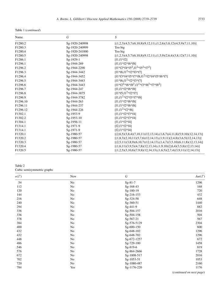
Table 2Cubic semisymmetric graphs

o(Γ ) New G Aut(Γ )

54 No Sg-81-7 1296112 No Sg-168-43 168120 No Sg-180-19 720144 No Sg-216-153 432216 No Sg-324-58 648240 No Sg-360-51 1440294 No Sg-441-9 882336 No Sg-504-157 2016336 No Sg-504-158 504378 No Sg-567-21 567384 No Sg-576-5129 2304400 No Sg-600-150 600432 No Sg-648-102 1296432 No Sg-648-702 1296448 No Sg-672-1257 672486 No Sg-729-100 1458546 No Sg-819-6 819576 No Sg-864-2666 1728672 No Sg-1008-517 2016702 No Sg-1053-51 1053720 No Sg-1080-487 2160784 Yes Sg-1176-220 1176

(continued on next page)

2734 A. Bretto, L. Gillibert / Discrete Applied Mathematics 156 (2008) 2719–2739

Table 2 (continued)

o(Γ ) New G Aut(Γ )

784 Yes Sg-1176-215 1176784 Yes Sg-1176-42 1176798 Yes Sg-1197-9 1197864 Yes Sg-1296-235 2592864 Yes Sg-1296-1803 5184882 Yes Sg-1323-21 2646896 Yes Sg-1344-815 1344896 Yes Sg-1344-816 1344896 Yes Sg-1344-11309 1344

1008 Yes Sg-1512-780 30241008 Yes Sg-1512-785 15121008 Yes Sg-1512-443 15121014 Yes Sg-1521-9 30421026 Yes Sg-1539-30 15391134 Yes Sg-1701-141 17011152 Yes Sg-1728-12488 69121152 Yes Sg-1728-20789 34561176 Yes Sg-1764-168 17641280 Yes Sg-1920-241001 38401296 Yes Sg-1944-3448 38881296 Yes Sg-1944-3452 38881296 Yes Sg-1944-3449 19441296 Yes Sg-1944-2290 19441302 Yes Sg-1953-6 19531320 Yes Sg-1980-57 7920

These two tables were built in 212 min on a 2 GHz Athlon (a 32 bit processor). The version of the Foster Censuscontaining cubic graphs up to the order 768 was built in a hundred hours on a 100 processors supercalculator [6]. Ifwe consider the tables up to the order 1320, all the cubic symmetric graphs are known. In this table, only 408 bipartitecubic symmetric graphs are not G-graphs. There are 446 bipartite cubic symmetric graphs up to the order 1320, so91.5% of them are G-graphs.

Notice that the following well-known cubic symmetric or semisymmetric graphs are G-graphs. The correspondinggroups are indicated between parentheses:

1. The cube

(G = A4, S = (1, 2, 3), (1, 3, 4)).

2. The Heawood graph

(〈a, b | a7= b3

= e, ab = baa〉, S = b, ba).

3. The Pappus graph

(G = 〈a, b, c | a3= b3

= c3= e, ab = ba, ac = ca, bc = cba〉, S = b, c).

4. The Mobius–Kantor graph

(G = Sg − 24 − 3, S = f 1, f 1 ∗ f 2).

5. The Gray graph

(G = Sg − 81 − 7, S = f 1, f 2).

6. The Ljubljana graph

(G = Sg − 168 − 43, S = f 1, f 1 ∗ f 2 ∗ f 4).

By the same process it is easy to establish some tables of quintic symmetric and semisymmetric G-graphs (seeTables 3 and 4).

A. Bretto, L. Gillibert / Discrete Applied Mathematics 156 (2008) 2719–2739 2735

Table 3Quintic semisymmetric G-graphs

O(Γ ) O(G) G Aut(Γ )

120 300 Sg-300-22 1200240 600 Sg-600-54 2400250 625 Sg-625-7 10000720 1800 Sg-1800-555 14400

Table 4Quintic symmetric G-graphs

O(Γ ) O(G) G Aut(Γ )

10 25 Sg-25-2 28 80022 55 Sg-55-1 1 32024 60 Sg-60-5 48032 80 Sg-80-49 3 84048 120 Sg-120-5 96050 125 Sg-125-3 4 00062 155 Sg-155-1 31064 160 Sg-160-199 64082 205 Sg-205-1 410

110 275 Sg-275-3 550122 305 Sg-305-1 610128 320 Sg-320-1012 2 560142 355 Sg-355-1 710144 360 Sg-360-118 5 760160 400 Sg-400-213 3 200162 405 Sg-405-15 19 440202 505 Sg-505-1 1 010242 605 Sg-605-1 1 210242 605 Sg-605-5 1 210242 605 Sg-605-6 2 420262 655 Sg-655-1 1 310264 660 Sg-660-13 5 280288 720 Sg-720-409 2 880302 755 Sg-755-1 1 510310 775 Sg-775-3 1 550320 800 Sg-800-1065 6 400352 880 Sg-880-214 1 760362 905 Sg-905-1 1 810382 955 Sg-955-1 1 910384 960 Sg-960-11357 7 680384 960 Sg-960-11358 46 080410 1025 Sg-1025-3 2 050422 1055 Sg-1055-1 2 110432 1080 Sg-1080-260 4 320482 1205 Sg-1205-1 2 410486 1215 Sg-1215-68 4 860502 1255 Sg-1255-1 2 510528 1320 Sg-1320-13 5 280542 1355 Sg-1355-1 2 710550 1375 Sg-1375-9 2 750562 1405 Sg-1405-1 2 810600 1500 Sg-1500-112 12 000610 1525 Sg-1525-3 3 050622 1555 Sg-1555-1 3 110640 1600 Sg-1600-6786 12 800

(continued on next page)

2736 A. Bretto, L. Gillibert / Discrete Applied Mathematics 156 (2008) 2719–2739

Table 4 (continued)

O(Γ ) O(G) G Aut(Γ )

662 1655 Sg-1655-1 3 310682 1705 Sg-1705-3 3 410682 1705 Sg-1705-4 3 410682 1705 Sg-1705-5 3 410682 1705 Sg-1705-6 3 410704 1760 Sg-1760-1139 3 520710 1775 Sg-1775-3 3 550722 1805 Sg-1805-2 7 220800 2000 Sg-2000-488 16 000

Fig. 5. The G-graph Φ(A4; S).

Fig. 6. L(Φ(A4; S)) is a CAYLEY graph.

5.2. Quartic graphs

By the implication (i) ⇒ (ii) of Theorem 2, the line-graph of a cubic G-graph is a quartic CAYLEY graph. Ourtable of cubic symmetric and semisymmetric G-graphs gives us a table of quartic CAYLEY graphs.

Example 3. Let G be the group sg-12-3 generated by a family S = a, b of size 2 with a3= b3

= e. Forinformation, the group named sg-12-3 is isomorphic to A4. The G-graph Φ(G; S) is a bipartite cubic graph (seeFig. 5).

It is a cubic symmetric G-graph on eight vertices isomorphic to the skeleton of a cube. If we compute the line-graphof the G-graph Φ(G; S) we find a quartic CAYLEY graph (see Fig. 6).

It is a symmetric quartic graph isomorphic to the cuboctahedral graph. It is also a G-graph generated by the groupG = C2 × C2 × C2.

6. An infinite family of symmetric G-graphs

6.1. Preliminaries

Let A be the ring Z/m.Z, m ≥ 1. We have GL(A) ' A× by the following isomorphism:

λ : A×−→ GL(A)

a 7−→ λa : x 7−→ a.x .

A. Bretto, L. Gillibert / Discrete Applied Mathematics 156 (2008) 2719–2739 2737

Hence |GL(A)| = φ(m). Let T = tb, b ∈ A, the group of translations; we have T ' (Z/m.Z,+) by

t : Z/m.Z −→ T

b 7−→ tb : x 7−→ x + b

and GL(A) and T are subgroups of Sym(A). It is well known [14] that Aff (A) = 〈T,GL(A)〉. Becauseλa tb λ−1

a = ta.b and GL(A) ∩ T = e we have: Aff (A) = T o GL(A). So |Aff (A)| = m.φ(m).

6.2. Group construction

Let a be in A× with an order equal to n such that n|φ(m). We have o(λa) = o(a) = n. Let h : x 7−→ a.x + 1,i.e. h = t1 λa , an element of Aff (A). Consider G = 〈h, λa〉 = 〈t1, λa〉 = 〈T, λa〉. From the remarks above we haveG = T o λa ; hence |G| = m.n. It is easy to see that

hs= t

1+a+a2+···+as−1 λsa . (1)

Let’s set k = min j ≥ 1, k.(1 + a + a2+ · · · + as−1) = 0, mod m. Because Z/m.Z is finite, k exists. Consequently

o(h) = k.n.

Remark. We have 0 = an− 1 = (a − 1)(an−1

+ an−2+ an−3

+ · · · + a + 1).

• If a, a − 1 ∈ A× in this case a 6= 1 and an−1+ an−2

+ an−3+ · · · + a + 1 = 0. Consequently k = 1.

• If m is prime, Z/m.Z is an integral domain, i.e. there are no zero divisors, and a 6= 1; hence an−1+an−2

+an−3+

· · · + a + 1 = 0 and k = 1.

Consequently |G| = |〈h, λa〉| = n.m with o(h) = o(λa) = n. Moreover if m is prime, A× is cyclic with orderequal to φ(m) = m − 1, so for any n divisor of m − 1 there is a ∈ A× with an order equal to n.

Assume that m is prime, m ≡ 1 mod 3; choose a ∈ A× with o(a) = n = 3, so |G| = |T o 〈λa〉| = 3.m. SetS = λa, h, with h = t1 λa .

Theorem 3. Let (G, S) be the group generated by S = λa, h defined above, and let Φ((G, S)) be the G-graphassociated with this group. This G-graph is symmetric.

Proof. We are going to show that there is τ ∈ Aut(G, S) such that:

• τ(λa) = h which have to have order equal to 3,• τ(h) = λa .

These automorphisms are completely determined by:

• τ(λa) which have to have order equal to 3,• τ(t1) which have to have order equal to m.

Because G is a semi-direct product we have to calculate the order of the elements x = tb λia . It is easy to show (by

induction) that ∀ i,∀ b: λia tb = tai b λi

a . Hence (or by applying (1)), we have (tb λia)

s= tb(1+a+a2+···+a(s−1)i ) λ

sia ;

so from this,

• o(tb) = m, for b 6= 0• o(tb λi

a) = 3, i ∈ 1, 2.

Consequently if there is an automorphism with the conditions defined below, this automorphism looks like:

• τ(λa) = tb λia , i ∈ 1, 2.

• τ(t1) = tb, b 6= 0.

Conversely, let α ∈ 1, 2 and for β, γ let us set:

• ψ(t1) = tβ , β 6= 0.• ψ(λa) = tγ λαa .

We have:

2738 A. Bretto, L. Gillibert / Discrete Applied Mathematics 156 (2008) 2719–2739

• ψ(tb) = tβ.b.• ψ(tb λi

a) = tβ.b+γ.(1+aα+···+a(i−1)α) λα.ia , i ∈ 1, 2.

Set:σ0 = 0σi = γ.(1 + aα + · · · + a(i−1)α).

We have ψ(tb λia) = tβ.b+σi λα.ia .

We have now to show that: for x = tb λia and y = tb′ λi ′

a , ψ(x .y) = ψ(x).ψ(y),

ψ(tb λia tb′ λi ′

a ) = ψ(tb tai .b′ λia tb′ λi ′

a ) = ψ(tb+ai .b′ λia tb′ λi ′

a ) = tβ.(b+ai .b′)+σi+i ′λ

α.(i+i ′)a

ψ(tb λia) ψ(tb′ λi ′

a ) = tβ.b+σi λα.ia tβ.b′+σi ′ λα.i

′

a = tβ.b+σi taα.i .(β.b′+σi ′ ) λα.ia λα.i

′

a .

So ψ(x .y) = ψ(x).ψ(y) if and only if β.(b + ai .b′) + σi+i ′ ≡ β.b + σi + aα.i .β.b′+ aα.i .σi ′; mod m

which is equivalent to β.ai .b′+ σi+i ′ ≡ β.aα.i .b′

+ σi + aα.i .σi ′; mod m. By definition, σi + aα.i .σi ′ =

γ.(1+aα+· · ·+a(i−1)α+aα.i ).γ .(1+aα+· · ·+a(i

′−1)α) = γ.(1+aα+· · ·+a(i−1)α

+aα.i +· · ·+a(i+i ′−1)α) = σi+i ′

Consequently, ψ(x .y) = ψ(x).ψ(y) if and only if ai .b′≡ aα.i .b′ mod m. Hence ai

= aα.i for all i . Consequentlyα = 1. So ψ(t1) = tβ and ψ(λa) = tγ λa , that leads to ψ = ψβ,γ : tb λi

a 7−→ tβ.b+σi λia from the definition of

ψ above.It is easy to check that ψ is an automorphism. Now we have to find an automorphism such that:

• ψ(λa) = h.• ψ(h) = λa .

ψ(λa) = ψ(t0 λa) = tσ1 λa = tγ λa = h = t1 λa implies that γ = 1.ψ(h) = ψ(t1 λa) = tβ+σ1 λa = λa implies that β = −σ1 or σ1 = γ . Consequently β = −1 = −γ . Hence

ψ(λa) = h and ψ(h) = λa with β = −1 and γ = 1 swap Vh and Vλa ; moreover from Theorem 4(c) δ(G) actstransitively on Vh and on Vλa ; consequently Φ((G; S)) is vertex-transitive.

7. Semisymmetric G-graphs

In this section we give a sufficient condition to show that a G-graph is semisymmetric. First we need the followingresult [2]:

Theorem 4. (1) Let us have (G; S) with S = s, t and 〈s〉 ∩ 〈t〉 = e, Φ(G; S) = (Vs t Vt ; E; ε). For g ∈ G wedefine δ(g) = (δg, δ

#g) by:

• δg((s)x) = (s)xg−1, s ∈ S, x ∈ G.• If e = ([(s)x, (t)y], u) ∈ E : δ#

g(e) = ([(s)xg−1, (t)yg−1], ug−1).

Hence we have the following properties:

(a) Φ(G; S) is a simple, bipartite, semi-regular connected graph.(b) 4 = δ(g), g ∈ G is a subgroup of AutpΦ(G; S).(c) 4 acts transitively on Vs , on Vt and on E.(d) For every v ∈ Vs t Vt , Stab4(v) is a cyclic group.

Conversely suppose Γ = (V1 t V2; E; ε) is a simple, bipartite, semi-regular connected graph with a subgroup 4

of AutpΓ such that:

(i) 4 is acting transitively on V1 and on V2.(ii) For every v ∈ V1 t V2, Stab4(v) is a non-trivial cyclic group.

(iii) 4 is acting transitively on E.(iv) There is an edge x1, x2 in Γ such that Stab4(x1) and Stab4(x2) are different and

o(G)

|Stab4x1|= |V1|,

o(G)

|Stab4x2|= |V2|.

Then there exists (G; S) such that Γ 'p Φ(G; S).

A. Bretto, L. Gillibert / Discrete Applied Mathematics 156 (2008) 2719–2739 2739

On the semisymmetric G-graphs we have the following result:

Proposition 4. Let Γ = Φ((G; S)) with S = s, t, 〈s〉 ∩ 〈t〉 = e and o(s) = o(t) ≥ 2. If Aut(Γ ) is a simple groupthen Γ is semisymmetric.

Proof. Let H = ϕ ∈ Aut(Γ ) : ϕ(Vs) = Vs and ϕ(Vt ) = Vt . H is a normal subgroup of Aut(Γ ) (since if σ ∈ Aut(Γ )and if x ∈ Vs with σ(x) ∈ Vt , necessarily σ(Vs) = Vt , by connectivity of Γ ). But H ⊃ 4 (cf. Theorem 4) and4 6= I dΓ ; hence Aut(Γ ) = H is not vertex-transitive.

References

[1] L. Babai, Automorphism groups, isomorphism, reconstruction, in: Handbook of Combinatorics, 1994 (Chapter 27).[2] A. Bretto, A. Faisant, L. Gillibert, G-graphs: A new representation of groups, Journal of Symbolic Computation 42 (5) (2007) 549–560.[3] A. Bretto, L. Gillibert, Symmetric and semisymmetric graphs construction using G-graphs, in: Proceedings of ISSAC’05, July 24–27, 2005,

Beijing, China, ACM Proceedings, 2005, pp. 61–67.[4] A. Bretto, L. Gillibert, Graphical and computational representation of groups, in: Proceedings of ICCS’2004, in: LNCS, vol. 3039, Springer-

Verlag, 2004, pp. 343–350.[5] I.Z. Bouwer, W.W. Chernoff, B. Monson, Z. Star, The Foster Census, Charles Babbage Research Centre, 1988.[6] Marston Conder, Peter Dobcsanyi, Trivalent symmetric graphs on up to 768 vertices, Journal of Combinatorial Mathematics and

Combinatorial Computing 40 (2002) 41–63.[7] Marston Conder, Aleksander Malnic, Dragan Marusic, Primoz Potocnik, A census of semi-symmetric cubic graphs on up to 768 vertices,

Journal of Algebraic Combinatorics 23 (2006) 255–294.[8] Marston Conder, All trivalent (cubic) symmetric graphs on up to 2048 vertices. On the web: http://www.math.auckland.ac.nz/˜conder/, 2006.[9] G. Cooperman, L. Finkelstein, N. Sarawagi, Applications of Cayley graphs, in: Appl. Algebra and Error-Correcting Codes, in: Lecture Notes

in Computer Sciences, vol. 508, Springer-Verlag, 1991, pp. 367–378.[10] J. Folkman, Regular line-symmetric graphs, Journal of Combinatory Theory 3 (1967) 215–232.[11] Joseph Lauri, Raffaele Scapellato, Topics in Graphs Automorphisms and Reconstruction. London Mathematical Society Student Texts, 2003.[12] Joseph Lauri, Constructing graphs with several pseudosimilar vertices or edges, Discrete Mathematics 267 (1–3) (2003) 197–211.[13] Brendan D. McKay, Practical graph isomorphism, Congressus Numerantium 30 (1981) 45–87.[14] Derek J.S. Robinson, A Course in the Theory of Groups, in: Springer-Verlag Graduate Texts in Mathematics, vol. 80, 1982.[15] Shaofei Du, M.Y. Xu, A classification of semisymmetric graphs of order 2pq , Communications in Algebra 28 (6) (2000) 2685–2715.[16] S. Lipschutz, M.Y. Xu, Note on infinite families of trivalent semisymmetric graphs, European Journal of Combinatorics 23 (2002) 707–711.[17] D. Marusic, Constructing cubic edge- but not vertex-transitive graphs, Journal of Graph Theory 35 (2000) 152–160.[18] A. Bretto, A. Faisant, A new way for associating a graph to a group, Mathematica Slovaca 55 (1) (2005) 1–8.