1

Symmetric Pseudo-Random MatricesIlya Soloveychik, Yu Xiang and Vahid Tarokh

John A. Paulson School of Engineering and Applied Sciences,Harvard University

Dedicated to the memory of Solomon W. Golomb (1932-2016)

Abstract—We consider the problem of generating sym-metric pseudo-random sign (+−1) matrices based on thesimilarity of their spectra to Wigner’s semicircular law.Using binary m-sequences (Golomb sequences) of lengthsn = 2m − 1, we give a simple explicit construction ofcirculant n× n sign matrices and show that their spectraconverge to the semicircular law when n grows. TheKolmogorov complexity of the proposed matrices equalsto that of Golomb sequences and is at most 2log2(n) bits.

Index Terms—Pseudo-random matrices, semicircularlaw, Wigner ensemble.

I. INTRODUCTION

A. Wigner Matrices: Universality and Structure

Random matrices have been a very active area ofresearch for the last few decades and have found enor-mous applications in various areas of modern mathe-matics, physics, engineering, biological modeling, andother fields [1]. In this article, we focus on the squaresymmetric matrices with +−1 entries, referred to as squaresymmetric sign matrices. For this model, Wigner [2]demonstrated that if the elements of the upper triangularpart (including the main diagonal) of an n×n matrix areindependent Rademacher (+−1 with equal probabilities)random variables, then as n grows a properly scaledempirical spectral measure converges to the semi-circlelaw. Originally, Wigner proved convergence in expecta-tion, but 3 years later he himself improved the resultto convergence in probability [3]. In about a decade,Arnold [4] strengthened the claim to almost sure weakconvergence.

After the pioneering works of Wigner and the in-ception of the Random Matrix Theory (RMT), a greatdeal of research effort was put into generalization ofthe original basic random matrix setup. The two maindirections of generalization can be roughly defined asuniversality and structure.

The universality phenomenon can be viewed as a non-commutative analog of the Central Limit Theorem [5], in

This work was supported by the Fulbright Foundation and ArmyResearch Office grant No. W911NF-15-1-0479.

other words, it can be understood as invariance of somelimiting properties of the matrices under a change ofthe marginal (atomic) distributions of the matrix entries,given that the independence conditions are left intact.In the last 20 years, much work have been devoted tothe analysis of the universality phenomena with regardto different matrix properties and of their exact bounds.Remarkably, when it comes to the semicircular limitingspectrum, necessary conditions on the marginal distribu-tions were quite well studied (see [6] and surveys [7, 8]).

In the second direction of the generalization endeavor,which we call structure or dependence, scientists tryto understand to what extent the tough independenceconditions on the matrix entries can be relaxed withoutaffecting the limiting behavior. The importance of thisline of research is hard to overestimate, as alreadyin the early applications of RMT, the validity of theindependence condition was questioned by a number ofworks coming mainly from physics and related fields[9, 10]. Unlike universality, very little is known abouthow much structure can one allow and still obtain anensemble with the semicircular limiting law. Some recentworks [11–13] allow moderate amount of dependencebetween matrix elements. Usually, the level of per-mitted structure is limited by the specific tools usedfor the analysis and to the best of our knowledge nounified examination of the information-theoretic boundsof the possible dependencies has been performed sofar. Moreover, due to the vagueness and complexity ofdetermining the dependencies between the entries andtheir quantitative assessment, there does not seem toexist literature specifically concentrating on this issueand rigorously introducing the system of reference forsuch study.

In this work, we will make an attempt towards abetter understanding of the amount of structure that canbe tolerated by the semicircular law. Below we resortto the Kolmogorov complexity paradigm to quantifythe dependencies between the matrix elements for signmatrices. We give an explicit construction of matriceswith substantial amount of structure whose spectra stillconverge to the semicircular law. Using general results

arX

iv:1

702.

0408

6v8

[m

ath.

PR]

26

Feb

2018

2

from the theory of algorithmic complexity, we justify thatthe measure of structure existing in our construction isclose to the maximal possible thus showing that indeeda large amount of dependence between the entries canbe introduced without affecting the limiting law.

B. Pseudo-random SequencesFrom a different perspective, in many engineering

applications one needs to simulate random matrices.The most natural way to generate an instance of arandom n × n sign matrix is to toss a fair coin n(n+1)

2times, fill the upper triangular part of a matrix withthe outcomes and reflect the upper triangular part intothe lower. Unfortunately, for large n such an approachwould require a powerful source of randomness due tothe independence condition [14]. In addition, when thedata is generated by a truly random source, atypical non-random looking outcomes have non-zero probability ofshowing up. Yet another issue is that any experimentinvolving tossing a coin would be impossible to repro-duce exactly. All these reasons stimulated researchersand engineers from different areas to seek for approachesof generating random-looking data usually referred toas pseudo-random sources or sequences of binary digits[15, 16]. A wide spectrum of pseudo-random numbergenerating algorithms have found applications in a largevariety of fields including radar, digital signal processing,CDMA, coding theory, cryptographic systems, MonteCarlo simulations, navigation systems, scrambling, etc.[15].

The term pseudo-random is used to emphasize thatthe binary data at hand is indeed generated by an en-tirely deterministic causal process with low algorithmiccomplexity, but its statistical properties resemble someof the properties of data generated by tossing a faircoin. Remarkably, most efforts were focused on onedimensional pseudo-random sequences [15, 16] due totheir natural applications and to the relative simplicityof their analytical treatment. One of the most popularmethods of generating pseudo-random sequences is dueto Golomb [16] and is based on linear-feedback shift reg-isters capable of generating pseudo-random sequences ofvery low algorithmic complexity. The study of pseudo-random arrays and matrices was launched around thesame time [17–20]. Among the known two dimensionalpseudo-random constructions the most popular are theso-called perfect maps [17, 21, 22], and the two di-mensional cyclic codes [19, 20]. However, except forour recent article [23] discussed below, to the best ofour knowledge none of the previous works consideredconstructions of symmetric matrices using their spectralproperties as the defining statistical features.

C. The Kolmogorov Complexity

There exist various approaches to quantify the algo-rithmic power needed to generate an individual piece ofbinary data, also known as algorithmic complexity [24–26]. It can be intuitively thought of as a measure of theamount of randomness stored in that piece of data. Prob-ably the most popular among computer theorists measureof algorithmic complexity is the so-called Kolmogorov(Kolmogorov-Chaitin) complexity [27, 28] defined asfollows. Let D be a string of binary data of length n, thenits Kolmogorov complexity is the length of the shortestbinary Turing machine code that can produce D and halt.If D has no computable regularity it cannot be encodedby a program shorter than its original length n (hereand below the Kolmogorov complexity is given up toan additive constant), meaning that its consecutive bitsare unpredictable given the preceding ones, and it maybe considered as truly random [25, 29]. A string with aregular pattern, on the other hand, can be computed by aprogram much shorter than the string itself, thus havinga much smaller Kolmogorov complexity. By convention,a comparison of Kolmogorov complexities of variousstrings of the same length is usually done by condition-ing on the length and thus assuming the length to bealready known to the machine without specifying it asan input [30]. For example, the conditional Kolmogorovcomplexity of a Golomb sequence of length n is atmost 2log2n, which is relatively small, since using asimple combinatorial argument one can show that at mostn2n fraction of the strings of length n have conditionalKolmogorov complexity less than log2n.

We would like to emphasize that the definition of theKolmogorov complexity does not require the data gener-ating algorithm to be presented explicitly, and thereforeis sometimes considered to be not very informative.There exist finer measures of algorithmic complexity tak-ing into account the level of explicitness of the algorithmand/or its run time [31]. The algorithm that we presentin this paper is in fact “very” explicit even accordingto demanding definitions of complexity or explicitness.However, to avoid deep digression into the subtleties ofdifferent definitions of algorithmic complexity due tolack of space, and in order not to deviate much fromthe main topic of the article, in this work we focus onKolmogorov complexity.

D. Spectral Pseudo-randomness

Most of the literature dealing with specific pseudo-random constructions start from a list of concrete prop-erties mimicking truly random data and try to come upwith a deterministic way of reproducing those properties.

3

We would like to adapt the same paradigm and apply itto the property of random matrices to have asymptot-ically semicircular spectral distribution. It is importantto emphasize that unlike the works listed above, wecannot require any single matrix to have semicircularspectral density, since the spectrum of a matrix is a stepfunction and cannot be smooth. Therefore, we need toadjust the framework to our case and allow matrices toonly approximately match the desired property, whilerequiring exact matching in the limit. This forces usto deal with sequences of matrices instead of singlerealizations. We concentrate on the problem of deter-ministically constructing sequences of symmetric signmatrices whose spectra converge to the semicircular law.A naturally arising question here may be formulatedas: “What is the minimal Kolmogorov complexity ofmatrices in a sequence of sign matrices, whose spectraconverge to the semicircular law?”. Yet another impor-tant question that have been challenging mathematicaland engineering society for the last decades is the inversespectral problem which can be formulated as: “What canbe said about a large sign matrix (an adjacency matrix ofa graph lifted by the mapping 0→ 1 and 1→ −1) if itsspectrum is known/is close to a semicircle?”. Based onthe experience with Wigner’s matrices and their spectralproperties scientists tend to believe that if the spectrumof a matrix is close to the semicircle, it will necessarylook random and will also possess no observable struc-ture. Unfortunately, there does not exist much literatureon this problem due to its complexity. In this article, wetry to shed some light on the aforementioned questions.

Using Golomb sequences (also known as binary m-sequences) of lengths n = 2m−1, we explicitly constructn×n symmetric circulant sign matrices of Kolmogorovcomplexity as low as 2log2n, whose spectra convergeto the semicircular law with n → ∞. The proof givenbelow follows the classical method of moments anddemonstrates that the empirical moments of a prop-erly designed ensemble of our pseudo-random matricesconverge almost surely to the correct limiting values,which implies almost surely weak convergences of theempirical distributions. This surprising result has at leastthree major consequences. First, it means that the realamount of randomness conveyed by the semicircular lawis quite low. Second, it provides the first deterministicconstruction of such matrices, which may significantlyaffect many applications where random matrices aregenerated using more powerful sources of randomness.Finally, it partially answers the inverse spectral problemby building a sequence of circulant structured matriceswith spectra converging to Wigner’s law, which contra-dicts the common belief that matrices with semicircular

spectrum must be random looking.The proposed construction can be viewed as a pseudo-

random analog of the truly random circulant model withindependent Rademacher entries. The empirical spectraof the truly random circulant matrices converge almostsurely to the normal law [32] having unbounded supportand, thus, being significantly different from the limitingdistribution in our case. This means in particular that theintrinsic structure of the Golomb sequences combinedwith the circulant pattern surprisingly boils down intothe semicircular law. This phenomenon requires furtherinvestigation and may contribute to the study of theinverse spectral problem. The only other known pseudo-random symmetric sign matrices with spectra convergingto the semicircular law are the elements of the pseudo-Wigner ensemble built from the dual BCH codes [23].Compared to that paper, our present model has a com-pletely deterministic and easier construction algorithmand lower algorithmic complexity. In addition, in thepresent work convergence of the empirical spectra tothe limiting law is shown to be almost sure, while inthe setup of [23] only convergence in probability can beguaranteed.

It can be easily observed that the second powersof our pseudo-random matrices provide a deterministicconstruction of matrices whose spectra converge to theMarchenko-Pastur law with the aspect ratio γ = 1 [33].The Marchenko-Pastur distribution naturally arises asthe limiting spectral density of high-dimensional samplecovariance matrices with independent samples undersome assumptions on the population distribution [33].The algorithmic complexity of the squared matrices isthe same as of the original ones up to a constant term,thus yeilding an efficient pseudo-random construction ofmatrices with the limiting Marchenko-Pastur spectrum.

E. Pseudo-random Graphs

It is also instructive to relate our pseudo-randommatrices to the numerous random-looking graphs mostlyconsidered in combinatorics and the theory of computerscience [34, 35]. Binary symmetric n × n matricesnaturally correspond to unweighted, undirected graphson n vertices, since each matrix element aij may beviewed as indicating the presence of the edge (i, j).Graphs mimicking properties of truly random graphsare mainly utilized for the purposes of derandomization,see [31, 34, 35] and references therein. Popular classesof random-looking graphs include pseudo-random (jum-bled) [36], quasi-random [37], expander graphs [31]and others. Remarkably, construction of some of themcan be very involved (e.g. expanders), limiting their

4

usage in high dimensions. In addition, in most pseudo-random graph constructions only results regarding theirtop eigenvalues are usually reported, leaving aside inves-tigation of the bulk of their spectra.

The rest of the text is organized as follows. First weintroduce notation in Section II. Section III is devotedto the brief overview of Golomb sequences and linear-feedback shift registers. Then we define the notionof pseudo-random matrices constructed from Golombsequences in Section IV and formulate the main resultsof the article regarding the convergence of their empiricalspectra to the semicircular distribution in Section V. InSection VI, we discuss the Kolmogorov complexity ofthe proposed matrices. The numerical simulations andcomparisons of our model with other related ensemblesare given in Section VII. All the auxiliary claims and theproofs of the main results are presented in Appendices.

II. NOTATION

Let C be a [n, k, d] binary linear code of length n,dimension k and minimum Hamming distance d. Thedual code C⊥ of C is a linear code of the same length anddimension k⊥ = n−k, whose codewords are orthogonalto all the codewords of C, where we say that two wordsu = {ui}, v = {vi} ∈ GF (2)n are orthogonal if∑

i viui = 0 mod 2. Introduce a family of functions

ζn : GF (2)n×n → {−1, 1}n×n,{uij}n−1i,j=0 7→ {(−1)uij}n−1i,j=0,

(1)

mapping binary 0/1 matrices into sign matrices of thesame sizes. Below we suppress the subscript and writeζ for simplicity.

We denote by Sn the set of all symmetric n × nmatrices with entries +− 1

2√n

. The Wigner ensemble Wn

is defined as the set Sn endowed with the uniformprobability measure. Ranges of non-negative integers aredenoted by [n] = {0, . . . , n − 1}. Note also that theinteger indexation of matrix elements starts with 0.

We use the following standard notation for the limitingrelations between functions. We write f(n) = o(g(n))

if limn→∞f(n)g(n) = 0 and f(n) = O(g(n)) if |f(n)| 6

C|g(n)| for some constant C and n big enough.

III. GOLOMB AND BINARY m-SEQUENCES

A. Golomb Sequences

Let f(x) be a binary primitive polynomial of degreem and let C be a cyclic code of length n = 2m− 1 withthe generating polynomial

h(x) =xn − 1

f(x). (2)

In other words,

C = {c ∈ GF (2)n | h(x)|c(x)}, (3)

where

c(x) =

n−1∑i=0

cixi. (4)

When f(x) is primitive, as in our case, a code con-structed in such a way is usually referred to as a simplexcode. All the non-zero codewords of the obtained codeare shifts of each other and are called Golomb sequences[16] (we can, therefore, simply say that a simplex codeis generated by a Golomb sequence). Note that thedual code of C, C⊥ is simply a binary Hamming codegenerated by f(x). The dimensions of C and C⊥ are mand n−m, correspondingly.

It is sometimes convenient to glue a few copies ofthe same codeword together and consider them as aperiodic sequence with the period at most n. Golombsequences have many desirable statistical properties.The best known of these properties claim that Golombsequences satisfy Golomb’s axioms for pseudo-randomsequences [16].

Let ϕ = {ϕ(i)}n−1i=0 be a periodic sequence, then thethree axioms for ϕ to be a pseudo-random sequence areas follows.

[G1] Distribution: In every period the number of ones isnearly equal to the number of zeros, more preciselythe difference between the two numbers is at most1 ∣∣∣∣∣

n−1∑i=0

(−1)ϕ(i)

∣∣∣∣∣ 6 1. (5)

[G2] Serial test I: A sequence of consecutive ones iscalled a block and a sequence of consecutive zerosis called a gap. A run is either a block or a gap.In every period, one half of the runs has length 1,one quarter of the runs has length 2, and so on,as long as the number of runs indicated by thesefractions is greater than 1. Moreover, for each ofthese lengths the number of blocks is equal to thenumber of gaps.

[G3] Auto-correlation: The auto-correlation function

C(a) =

n−1∑i=0

(−1)ϕ(i)+ϕ(i+a) (6)

is two-valued.The distribution axiom [G1] is a special case of the

serial test axiom [G2]. However, [G1] is retained forhistorical reasons, and sequences which satisfy [G1] and[G3], but not [G2], are also important.

5

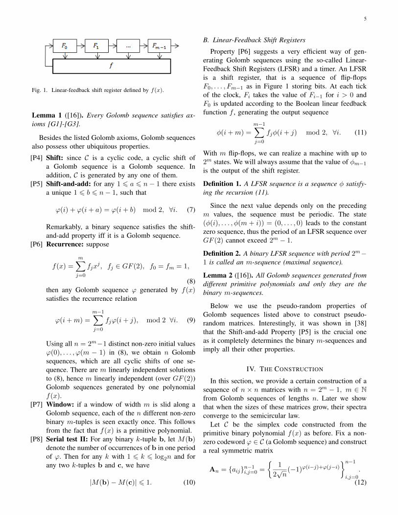
Fig. 1. Linear-feedback shift register defined by f(x).

Lemma 1 ([16]). Every Golomb sequence satisfies ax-ioms [G1]-[G3].

Besides the listed Golomb axioms, Golomb sequencesalso possess other ubiquitous properties.

[P4] Shift: since C is a cyclic code, a cyclic shift ofa Golomb sequence is a Golomb sequence. Inaddition, C is generated by any one of them.

[P5] Shift-and-add: for any 1 6 a 6 n− 1 there existsa unique 1 6 b 6 n− 1, such that

ϕ(i) + ϕ(i+ a) = ϕ(i+ b) mod 2, ∀i. (7)

Remarkably, a binary sequence satisfies the shift-and-add property iff it is a Golomb sequence.

[P6] Recurrence: suppose

f(x) =

m∑j=0

fjxj , fj ∈ GF (2), f0 = fm = 1,

(8)then any Golomb sequence ϕ generated by f(x)satisfies the recurrence relation

ϕ(i+m) =

m−1∑j=0

fjϕ(i+ j), mod 2 ∀i. (9)

Using all n = 2m−1 distinct non-zero initial valuesϕ(0), . . . , ϕ(m − 1) in (8), we obtain n Golombsequences, which are all cyclic shifts of one se-quence. There are m linearly independent solutionsto (8), hence m linearly independent (over GF (2))Golomb sequences generated by one polynomialf(x).

[P7] Window: if a window of width m is slid along aGolomb sequence, each of the n different non-zerobinary m-tuples is seen exactly once. This followsfrom the fact that f(x) is a primitive polynomial.

[P8] Serial test II: For any binary k-tuple b, let M(b)denote the number of occurrences of b in one periodof ϕ. Then for any k with 1 6 k 6 log2n and forany two k-tuples b and c, we have

|M(b)−M(c)| 6 1. (10)

B. Linear-Feedback Shift Registers

Property [P6] suggests a very efficient way of gen-erating Golomb sequences using the so-called Linear-Feedback Shift Registers (LFSR) and a timer. An LFSRis a shift register, that is a sequence of flip-flopsF0, . . . , Fm−1 as in Figure 1 storing bits. At each tickof the clock, Fi takes the value of Fi−1 for i > 0 andF0 is updated according to the Boolean linear feedbackfunction f , generating the output sequence

φ(i+m) =

m−1∑j=0

fjφ(i+ j) mod 2, ∀i. (11)

With m flip-flops, we can realize a machine with up to2m states. We will always assume that the value of φm−1is the output of the shift register.

Definition 1. A LFSR sequence is a sequence φ satisfy-ing the recursion (11).

Since the next value depends only on the precedingm values, the sequence must be periodic. The state(φ(i), . . . , φ(m + i)) = (0, . . . , 0) leads to the constantzero sequence, thus the period of an LFSR sequence overGF (2) cannot exceed 2m − 1.

Definition 2. A binary LFSR sequence with period 2m−1 is called an m-sequence (maximal sequence).

Lemma 2 ([16]). All Golomb sequences generated fromdifferent primitive polynomials and only they are thebinary m-sequences.

Below we use the pseudo-random properties ofGolomb sequences listed above to construct pseudo-random matrices. Interestingly, it was shown in [38]that the Shift-and-add Property [P5] is the crucial oneas it completely determines the binary m-sequences andimply all their other properties.

IV. THE CONSTRUCTION

In this section, we provide a certain construction of asequence of n × n matrices with n = 2m − 1, m ∈ Nfrom Golomb sequences of lengths n. Later we showthat when the sizes of these matrices grow, their spectraconverge to the semicircular law.

Let C be the simplex code constructed from theprimitive binary polynomial f(x) as before. Fix a non-zero codeword ϕ ∈ C (a Golomb sequence) and constructa real symmetric matrix

An = {aij}n−1i,j=0 =

{1

2√n

(−1)ϕ(i−j)+ϕ(j−i)}n−1i,j=0

.

(12)

6

Matrix An can be interpreted in the following way.Consider a circulant non-symmetric matrix

T =

ϕ(0) ϕ(1) ϕ(2) . . . ϕ(n− 1)

ϕ(n− 1) ϕ(0) ϕ(1) . . . ϕ(n− 2)ϕ(n− 2) ϕ(n− 1) ϕ(0) . . . ϕ(n− 3)

......

.... . .

...ϕ(1) ϕ(2) ϕ(3) . . . ϕ(0)

.

(13)The consecutive rows of T are simply cyclic shifts of theGolomb sequence written in its first rows. The symmetricmatrix An can now be written as

An =1

2√nζ(T + T>). (14)

It is easy to check that the obtained matrix is circulant,since for any k ∈ [n], An is invariant under the shift ofindices of the form

i→ i+ k mod n, j → j + k mod n. (15)

Recall that any non-zero codeword of C is a cyclicshift of ϕ, therefore, we may obtain an ensemble ofmatrices from the code C indexed by integers within therange a ∈ [n], as

An(a) =

{1

2√n

(−1)ϕ(i−j+a)+ϕ(j−i+a)}n−1i,j=0

, (16)

with the original matrix An corresponding to An(0).

Definition 3. Given a primitive binary polynomial f(x),an ensemble of pseudo-random matrices An of order nis the set of all An(a), a ∈ [n] and their negatives,endowed with the uniform probability measure.

Below, whenever expectation over An is consideredit should be always treated with respect to the uniformmeasure over An.

V. THE SPECTRA OF THE PSEUDO-RANDOM

MATRICES

In this section, we demonstrate that the spectra ofmatrices An uniformly chosen from An converge almostsurely to the semicircular law when their sizes grow toinfinity. We start from a number of auxiliary definitionsand results.

A. Wigner’s Ensemble and the Semicircular Law

For a real symmetric matrix An ∈ Sn, denote by

λ1(An) 6 · · · 6 λn(An) (17)

its eigenvalues, which are all real. Let FAnbe the

cumulative density function (c.d.f.) associated with thespectrum of An,

FAn(x) =

1

n

n∑i=1

θ (x− λi(An)) , (18)

where θ(x) is the unit step function at zero. The r-thmoment of An reads as

βr(An) =

∫xrdFAn

=1

nTr (Ar

n) . (19)

Denote by Fsc the c.d.f. of the standard semicircular law

Fsc(x) =1

2+

1

πx√

1− x2 +1

πarcsin(x),

− 1 6 x 6 1, (20)

and the corresponding probability density function(p.d.f.) by

fsc(x) =2

π

√1− x2, −1 6 x 6 1. (21)

The moments of this distribution read as [2]

βr =

∫xrdFsc =

{0, r odd,Cr/2

2r , r even,(22)

where

Cr =(2r)!

r!(r + 1)!(23)

is the r-th Catalan number. When the sizes of Wignermatrices grow, their moments converge to those ofthe semicircular law and their variances are summable,which ensures the almost sure convergence to the semi-circular law as stated by the following

Lemma 3 ([2, 4], Theorem 2.5 from [39]). Let Wn ∈Wn, then as n tends to infinity,

E [βr(Wn)] =

{βr + o(1), r even,

0, r odd,(24)

and for the variances of βr(Wn),

var (βr(Wn)) = O

(1

n2

). (25)

Corollary 1 ([4], Theorem 2.5 from [39]). The empiricalspectra of matrices from Wigner’s ensemble convergealmost surely weakly to the semicircular law.

Proof. Follows from Lemma 3 using Chebyshev’s in-equality and the Borel-Cantelli Lemma.

7

B. Spectrum of the Pseudo-random Construction

In the next two lemmas, we show an analog of Lemma3 for the proposed pseudo-random matrices which wouldguarantee the almost sure weak convergence of theirspectra to the semicircular law.

Proposition 1. Let An ∈ An, then for a fixed r ∈ Nand n = n(m) tending to infinity,

E [βr(An)] =

{βr +O

(1n

), r even,

0, r odd.(26)

Proof. The proof can be found in Appendix C.

Proposition 2. Let An ∈ An, then for a fixed r ∈ Nand n = n(m) tending to infinity,

var (βr(An)) = O

(1

n2

). (27)

Proof. The proof can be found in Appendix C.

Corollary 2. The empirical spectra of matrices An ∈An converge almost surely weakly to the semicircularlaw.

Proof. Follows from Propositions 1 and 2 through thesame argument as in the proof of Corollary 1.

Remark 1. In fact, we believe that even a stronger resultholds. Namely, that the empirical spectra of matrices An

converge to the semicircular law when n grows. Thisstatement does not involve probability and averagingover an ensemble, which may make it harder to beproved.

This surprising result has a number of consequences.First, it provides a deterministic construction of matriceswhose spectra converge to the semicircular law andshows that such matrices may be constructed with thehelp of a simple algorithm. In Section VI, we exactlyquantify the algorithmic complexity of the proposedconstruction. Second, unlike the common belief thatmatrices whose spectra converge to the semicircular lawmust be random-looking, it shows that this is not the caseand they may in fact be very structured. In particular, thepseudo-random family of matrices we suggest consistsof circulant matrices commuting with each other and,therefore, having a common fixed eigenbasis (this basiscan be easily obtained from a discrete Fourier matrix).

C. Relation to the Marchenko-Pastur Law

Interestingly, the above construction also enables us tobuild a sequence of pseudo-random matrices whose em-

pirical spectral distributions converge to the Marchenko-Pasur law defined through its p.d.f. as

fMP (x; γ) =1

2πγx

√(a+ − x)(x− a−), (28)

a− 6 x 6 a+,

where a± = (1 ± √γ)2 and γ is the so-called aspectratio parameter. Distribution (28) naturally appears as thelimiting spectral law of the sample covariance matricesof mn i.i.d. (independent and identically distributed)isotropic n-dimensional samples with

γ = limn→∞

mn

n6 1, (29)

under some additional conditions on the population dis-tribution [33, 40]. As a direct corollary of the main resultfrom the seminal work [33] of Marchenko and Pastur weget the following statement.

Lemma 4 (Corollary of Theorem 1 from [33]). Letfor every n ∈ N, {xij}mn−1,n−1

i,j=0 be i.i.d. Rademacherrandom variables and denote

Xmn,n =

{1√nxij

}mn−1,n−1

i,j=0

, (30)

then the empirical spectra of the sample covariancematrices Xmn,nX

>mn,n converge almost surely weakly to

the Marchenko-Pastur law with aspect ratio γ.

As a corollary of Propositions 1 and 2, we get

Corollary 3. The empirical spectra of matrices 4A2n

with An ∈ An converge almost surely weakly to theMarchenko-Pastur law with γ = 1.

Proof. The moments of the Marchenko-Pastur distribu-tion are given by the formula

ηr(γ) =

∫xrfMP (x; γ)dx =

r∑k=1

γkN(r, k), (31)

whereN(r, k) =

1

r

(k

r

)(k − 1

r

)(32)

are Narayana numbers. Use the identity

Cr =

r∑k=1

N(r, k) (33)

relating Narayana and Catalan numbers to conclude thatfor γ = 1,

ηr(1) =

r∑k=1

N(r, k) = Cr. (34)

The r-th moment of 4A2n is exactly the 2r-th moment

of 2An and since the latter converges almost surely to

8

the Catalan number Cr as follows from Propositions 1and 2, we get the desired statement.

Similarly to Wigner’s case, this surprising result sug-gests that even in cases where the measurements at hand(the columns of Xmn,n) are significantly dependent,the limiting distribution may still remain to be theMarchenko-Pastur law. In our current work, we aimat designing deterministic examples of matrices whosespectra converge to the Marchenko-Pastur distributionwith arbitrary aspect ratio.

VI. ALGORITHMIC COMPLEXITY OF THE

CONSTRUCTION

The standard computer scientific approach to quantifythe amount of randomness contained in a piece of dataD, also known as its algorithmic compressibility, isbased on calculating the length of a minimal programcreating that data on a universal Turing machine. Thelength of the obtained binary code is referred to as theKolmogorov complexity of the object and we denoteit by KC(D). A more fair comparison of Kolmogorovcomplexities of various objects of the same size isusually done by conditioning on that size KC(D|size),or in other words by assuming that it is already knownto the machine [30].

One may argue that measuring randomness of datasamples through the concept of Kolmogorov complexityis not particularly useful since Kolmogorov complexity isnot computable even using infinite computing resources.Indeed, it is a consequence of the fact that the haltingproblem for Turing machines is undecidable [41], thatit is theoretically impossible, not only computationallyinfeasible, to check all possible generation algorithmsfor a given piece of data and to choose the shortestamong them. To bypass this problem researchers andengineers often resort to the notion of linear complexity,which similarly to Kolmogorov complexity seeks forthe shortest program, however, restricts the search tothe class of LFSR-s. This restriction of the domain ofsearch makes linear complexity easily computable thanksto the Berlekamp-Massey algorithm [42, 43], which canfind the shortest LFSR generating a given binary string.Apparently, linear complexity always upper bounds theKolmogorov complexity.

Since we focus on circulant matrices, the wholeconstruction essentially reduces to the description ofthe first row. Due to equation (12), the first row of apseudo-random matrix at hand is constructed from asingle Golomb sequence. Therefore, up to a constantlength code describing the pattern of the matrix, thealgorithmic complexity of a pseudo-random n×n matrix

is that of a Golomb sequence ϕ of length n. The linearcomplexity of a Golomb sequence is easily computablesince by Lemma 2 they are exactly the binary m-sequences. To generate a Golomb sequence of lengthn = 2m − 1 we need to specify the associated primitivebinary polynomial of degree m, which requires at mostm− 1 bits (recall that its m-th and 0-th coefficients arealways 1) and the initial state of the register, the so-called seed, of m bits. Overall, the linear complexity ofa Golomb sequence is at most 2m−1 = 2log2(n+1)−1,which is asymptotically equivalent to

2log2(n+ 1)− 1 � 2log2n. (35)

Thus, we have proven the following result.

Proposition 3. The Kolmogorov complexity of thepseudo-random matrices from (12) is bounded by

KC(An|n) = KC(ϕ|n) + c

6 2log2(n+ 1)− 1 + c � 2log2n. (36)

Summarizing, Corollary 2 demonstrates that thereexist matrices with empirical spectra converging tothe semicircular law whose Kolmogorov complexity isasymptotically as low as 2log2n. To get an intuition ofhow small this value is, it is instructive to compare itwith the following classical result.

Lemma 5 ([25]). At most n2n fraction of all binary

strings of length n have conditional Kolmogorov com-plexity less than log2n.

This allows us to claim that the randomness require-ments for the semicircular law are comparatively small.In Section VII-D, we compare the proposed constructionto pseudo-Wigner matrices defined in [23].

It is important to emphasize that the Kolmogorovcomplexity alone does not entirely capture the powerof a sequence of matrices to approximate the limitingspectral law. Indeed, given a sequence of matrices wecan always dilute it by inserting other matrices betweenthe elements to get a sequence with lower algorithmiccomplexity but worse convergence properties. Therefore,a more objective comparison should consider the Kol-mogorov complexity versus the speed of convergence ofthe empirical measure to the limiting law in some metric.For example, let us consider the variance of the approxi-mation as such measure of error. As justified in Remarks2 and 3 in Appendix C, in both Wigner’s original caseand our pseudo-random construction, the decay of thevariance is of the same order 1

n2 as a function of thesize. However, the Kolmogorov complexity of a typicalmatrix from Wigner’s ensemble is equal to n(n+1)

2 up to

9

an additive constant [25], whereas the complexity of ourconstruction is at most 2log2n.

VII. NUMERICAL SIMULATIONS AND RELATED

MODELS

In this section we justify the above construction nu-merically and compare it to related constructions, bothrandom and pseudo-random.

A. Numerical Experiments

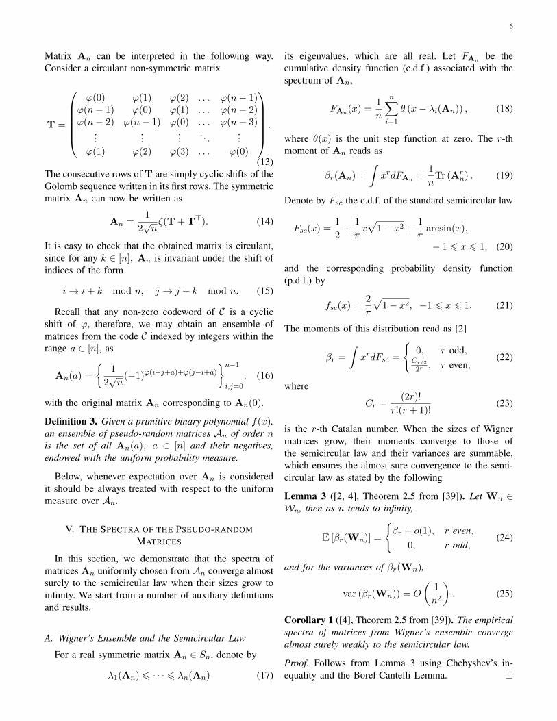
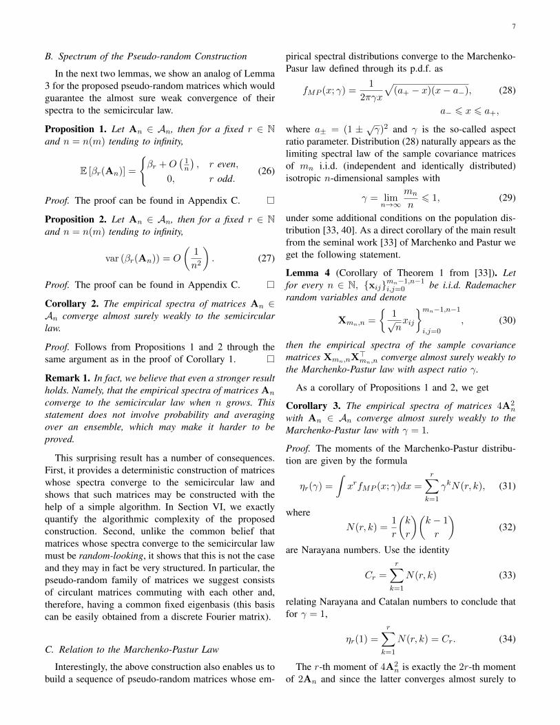
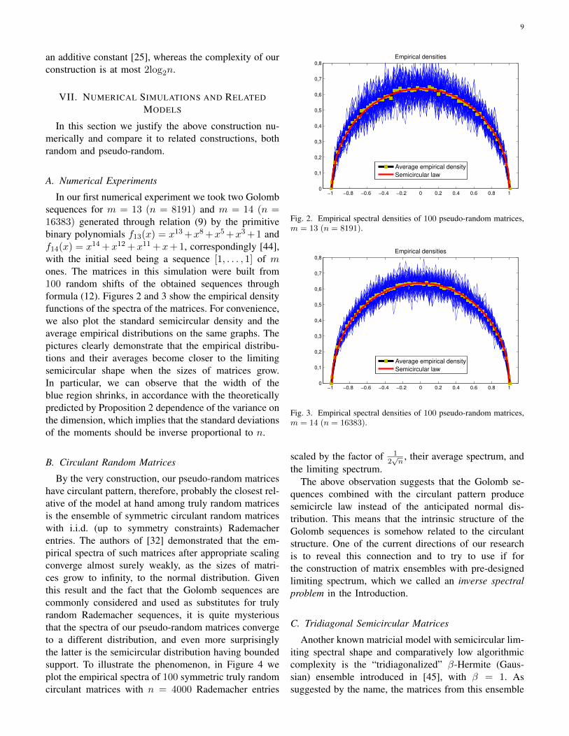
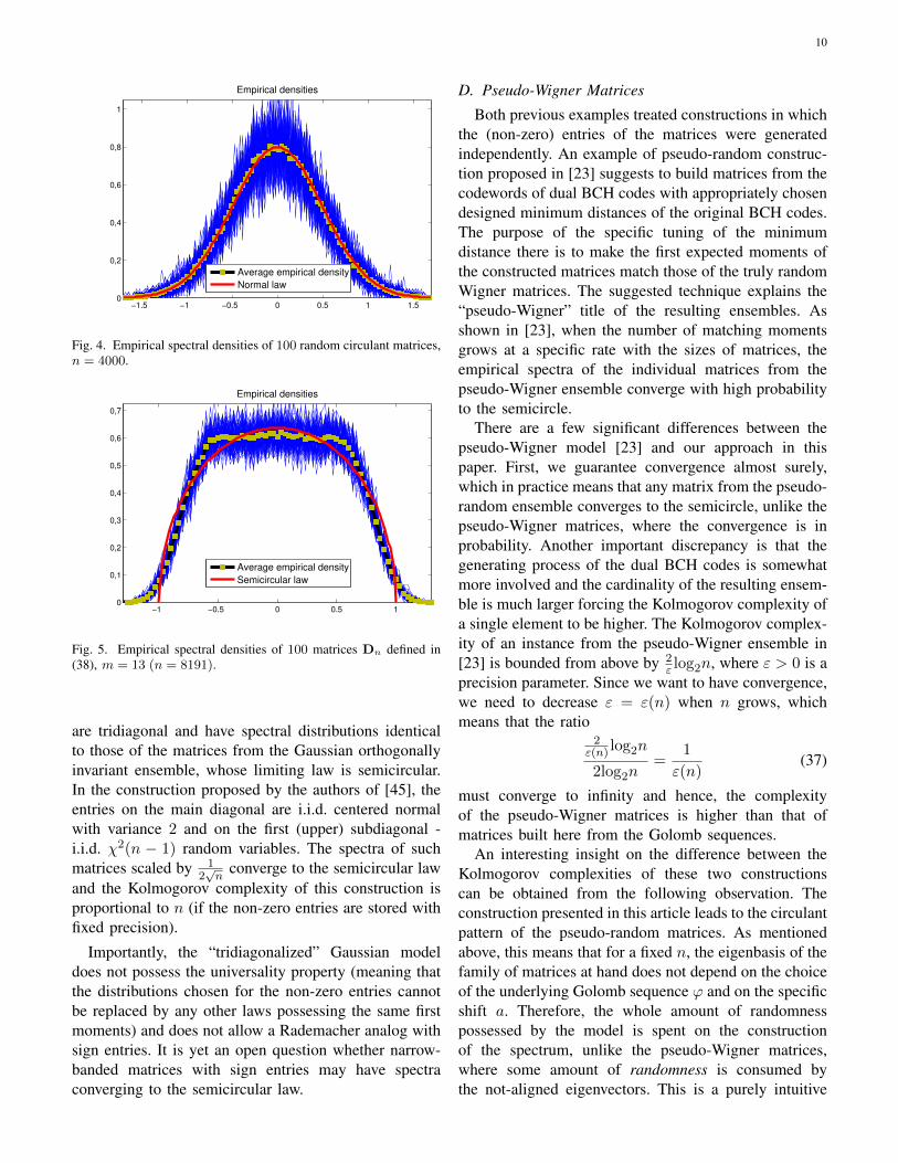
In our first numerical experiment we took two Golombsequences for m = 13 (n = 8191) and m = 14 (n =16383) generated through relation (9) by the primitivebinary polynomials f13(x) = x13 +x8 +x5 +x3 +1 andf14(x) = x14 +x12 +x11 +x+ 1, correspondingly [44],with the initial seed being a sequence [1, . . . , 1] of mones. The matrices in this simulation were built from100 random shifts of the obtained sequences throughformula (12). Figures 2 and 3 show the empirical densityfunctions of the spectra of the matrices. For convenience,we also plot the standard semicircular density and theaverage empirical distributions on the same graphs. Thepictures clearly demonstrate that the empirical distribu-tions and their averages become closer to the limitingsemicircular shape when the sizes of matrices grow.In particular, we can observe that the width of theblue region shrinks, in accordance with the theoreticallypredicted by Proposition 2 dependence of the variance onthe dimension, which implies that the standard deviationsof the moments should be inverse proportional to n.

B. Circulant Random Matrices

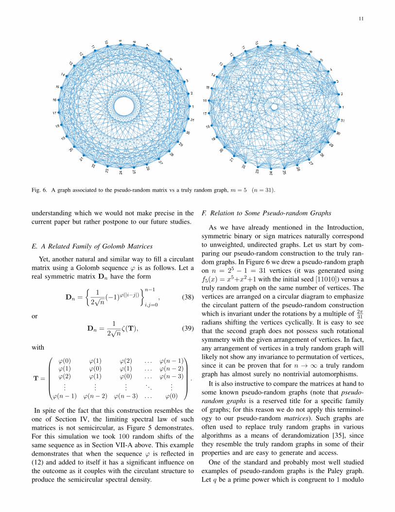
By the very construction, our pseudo-random matriceshave circulant pattern, therefore, probably the closest rel-ative of the model at hand among truly random matricesis the ensemble of symmetric circulant random matriceswith i.i.d. (up to symmetry constraints) Rademacherentries. The authors of [32] demonstrated that the em-pirical spectra of such matrices after appropriate scalingconverge almost surely weakly, as the sizes of matri-ces grow to infinity, to the normal distribution. Giventhis result and the fact that the Golomb sequences arecommonly considered and used as substitutes for trulyrandom Rademacher sequences, it is quite mysteriousthat the spectra of our pseudo-random matrices convergeto a different distribution, and even more surprisinglythe latter is the semicircular distribution having boundedsupport. To illustrate the phenomenon, in Figure 4 weplot the empirical spectra of 100 symmetric truly randomcirculant matrices with n = 4000 Rademacher entries

−1 −0.8 −0.6 −0.4 −0.2 0 0.2 0.4 0.6 0.8 10

0,1

0,2

0,3

0,4

0,5

0,6

0,7

0,8

Empirical densities

Average empirical density

Semicircular law

Fig. 2. Empirical spectral densities of 100 pseudo-random matrices,m = 13 (n = 8191).

−1 −0.8 −0.6 −0.4 −0.2 0 0.2 0.4 0.6 0.8 10

0,1

0,2

0,3

0,4

0,5

0,6

0,7

0,8

Empirical densities

Average empirical density

Semicircular law

Fig. 3. Empirical spectral densities of 100 pseudo-random matrices,m = 14 (n = 16383).

scaled by the factor of 12√n

, their average spectrum, andthe limiting spectrum.

The above observation suggests that the Golomb se-quences combined with the circulant pattern producesemicircle law instead of the anticipated normal dis-tribution. This means that the intrinsic structure of theGolomb sequences is somehow related to the circulantstructure. One of the current directions of our researchis to reveal this connection and to try to use if forthe construction of matrix ensembles with pre-designedlimiting spectrum, which we called an inverse spectralproblem in the Introduction.

C. Tridiagonal Semicircular Matrices

Another known matricial model with semicircular lim-iting spectral shape and comparatively low algorithmiccomplexity is the “tridiagonalized” β-Hermite (Gaus-sian) ensemble introduced in [45], with β = 1. Assuggested by the name, the matrices from this ensemble

10

−1.5 −1 −0.5 0 0.5 1 1.50

0,2

0,4

0,6

0,8

1

Empirical densities

Average empirical density

Normal law

Fig. 4. Empirical spectral densities of 100 random circulant matrices,n = 4000.

−1 −0.5 0 0.5 10

0,1

0,2

0,3

0,4

0,5

0,6

0,7

Empirical densities

Average empirical density

Semicircular law

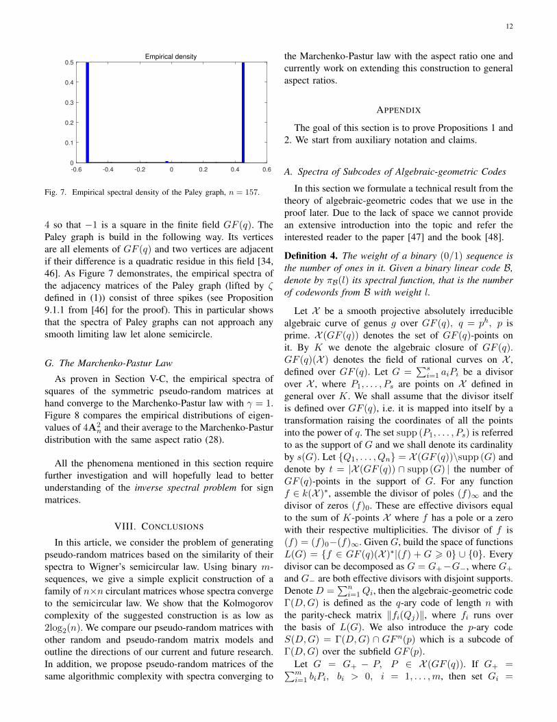
Fig. 5. Empirical spectral densities of 100 matrices Dn defined in(38), m = 13 (n = 8191).

are tridiagonal and have spectral distributions identicalto those of the matrices from the Gaussian orthogonallyinvariant ensemble, whose limiting law is semicircular.In the construction proposed by the authors of [45], theentries on the main diagonal are i.i.d. centered normalwith variance 2 and on the first (upper) subdiagonal -i.i.d. χ2(n − 1) random variables. The spectra of suchmatrices scaled by 1

2√n

converge to the semicircular lawand the Kolmogorov complexity of this construction isproportional to n (if the non-zero entries are stored withfixed precision).

Importantly, the “tridiagonalized” Gaussian modeldoes not possess the universality property (meaning thatthe distributions chosen for the non-zero entries cannotbe replaced by any other laws possessing the same firstmoments) and does not allow a Rademacher analog withsign entries. It is yet an open question whether narrow-banded matrices with sign entries may have spectraconverging to the semicircular law.

D. Pseudo-Wigner Matrices

Both previous examples treated constructions in whichthe (non-zero) entries of the matrices were generatedindependently. An example of pseudo-random construc-tion proposed in [23] suggests to build matrices from thecodewords of dual BCH codes with appropriately chosendesigned minimum distances of the original BCH codes.The purpose of the specific tuning of the minimumdistance there is to make the first expected moments ofthe constructed matrices match those of the truly randomWigner matrices. The suggested technique explains the“pseudo-Wigner” title of the resulting ensembles. Asshown in [23], when the number of matching momentsgrows at a specific rate with the sizes of matrices, theempirical spectra of the individual matrices from thepseudo-Wigner ensemble converge with high probabilityto the semicircle.

There are a few significant differences between thepseudo-Wigner model [23] and our approach in thispaper. First, we guarantee convergence almost surely,which in practice means that any matrix from the pseudo-random ensemble converges to the semicircle, unlike thepseudo-Wigner matrices, where the convergence is inprobability. Another important discrepancy is that thegenerating process of the dual BCH codes is somewhatmore involved and the cardinality of the resulting ensem-ble is much larger forcing the Kolmogorov complexity ofa single element to be higher. The Kolmogorov complex-ity of an instance from the pseudo-Wigner ensemble in[23] is bounded from above by 2

ε log2n, where ε > 0 is aprecision parameter. Since we want to have convergence,we need to decrease ε = ε(n) when n grows, whichmeans that the ratio

2ε(n) log2n

2log2n=

1

ε(n)(37)

must converge to infinity and hence, the complexityof the pseudo-Wigner matrices is higher than that ofmatrices built here from the Golomb sequences.

An interesting insight on the difference between theKolmogorov complexities of these two constructionscan be obtained from the following observation. Theconstruction presented in this article leads to the circulantpattern of the pseudo-random matrices. As mentionedabove, this means that for a fixed n, the eigenbasis of thefamily of matrices at hand does not depend on the choiceof the underlying Golomb sequence ϕ and on the specificshift a. Therefore, the whole amount of randomnesspossessed by the model is spent on the constructionof the spectrum, unlike the pseudo-Wigner matrices,where some amount of randomness is consumed bythe not-aligned eigenvectors. This is a purely intuitive

11

Fig. 6. A graph associated to the pseudo-random matrix vs a truly random graph, m = 5 (n = 31).

understanding which we would not make precise in thecurrent paper but rather postpone to our future studies.

E. A Related Family of Golomb Matrices

Yet, another natural and similar way to fill a circulantmatrix using a Golomb sequence ϕ is as follows. Let areal symmetric matrix Dn have the form

Dn =

{1

2√n

(−1)ϕ(|i−j|)}n−1i,j=0

, (38)

or

Dn =1

2√nζ(T), (39)

with

T =

ϕ(0) ϕ(1) ϕ(2) . . . ϕ(n− 1)ϕ(1) ϕ(0) ϕ(1) . . . ϕ(n− 2)ϕ(2) ϕ(1) ϕ(0) . . . ϕ(n− 3)

......

.... . .

...ϕ(n− 1) ϕ(n− 2) ϕ(n− 3) . . . ϕ(0)

.

In spite of the fact that this construction resembles theone of Section IV, the limiting spectral law of suchmatrices is not semicircular, as Figure 5 demonstrates.For this simulation we took 100 random shifts of thesame sequence as in Section VII-A above. This exampledemonstrates that when the sequence ϕ is reflected in(12) and added to itself it has a significant influence onthe outcome as it couples with the circulant structure toproduce the semicircular spectral density.

F. Relation to Some Pseudo-random Graphs

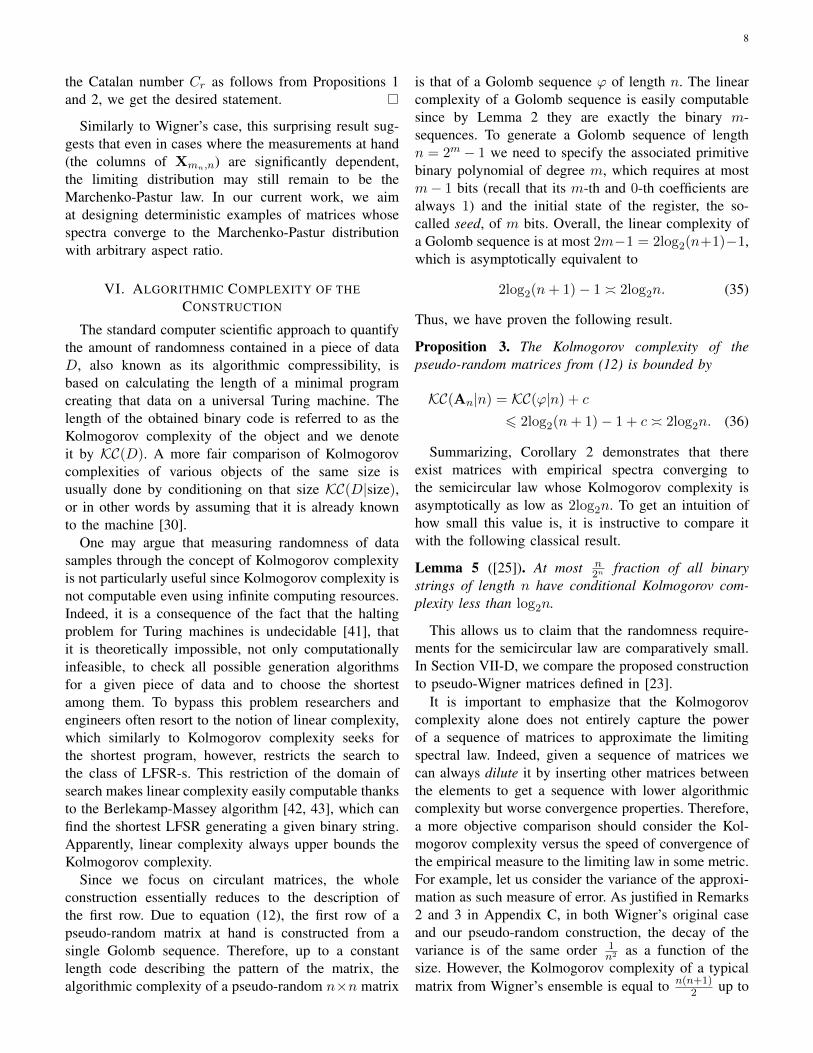
As we have already mentioned in the Introduction,symmetric binary or sign matrices naturally correspondto unweighted, undirected graphs. Let us start by com-paring our pseudo-random construction to the truly ran-dom graphs. In Figure 6 we drew a pseudo-random graphon n = 25 − 1 = 31 vertices (it was generated usingf5(x) = x5+x2+1 with the initial seed [11010]) versus atruly random graph on the same number of vertices. Thevertices are arranged on a circular diagram to emphasizethe circulant pattern of the pseudo-random constructionwhich is invariant under the rotations by a multiple of 2π

31radians shifting the vertices cyclically. It is easy to seethat the second graph does not possess such rotationalsymmetry with the given arrangement of vertices. In fact,any arrangement of vertices in a truly random graph willlikely not show any invariance to permutation of vertices,since it can be proven that for n → ∞ a truly randomgraph has almost surely no nontrivial automorphisms.

It is also instructive to compare the matrices at hand tosome known pseudo-random graphs (note that pseudo-random graphs is a reserved title for a specific familyof graphs; for this reason we do not apply this terminol-ogy to our pseudo-random matrices). Such graphs areoften used to replace truly random graphs in variousalgorithms as a means of derandomization [35], sincethey resemble the truly random graphs in some of theirproperties and are easy to generate and access.

One of the standard and probably most well studiedexamples of pseudo-random graphs is the Paley graph.Let q be a prime power which is congruent to 1 modulo

12

Empirical density

-0.6 -0.4 -0.2 0 0.2 0.4 0.60

0.1

0.2

0.3

0.4

0.5

Fig. 7. Empirical spectral density of the Paley graph, n = 157.

4 so that −1 is a square in the finite field GF (q). ThePaley graph is build in the following way. Its verticesare all elements of GF (q) and two vertices are adjacentif their difference is a quadratic residue in this field [34,46]. As Figure 7 demonstrates, the empirical spectra ofthe adjacency matrices of the Paley graph (lifted by ζdefined in (1)) consist of three spikes (see Proposition9.1.1 from [46] for the proof). This in particular showsthat the spectra of Paley graphs can not approach anysmooth limiting law let alone semicircle.

G. The Marchenko-Pastur Law

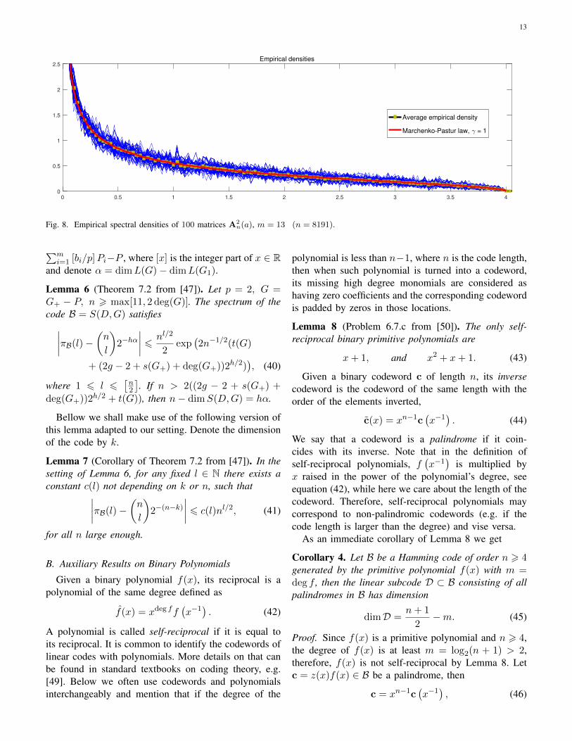
As proven in Section V-C, the empirical spectra ofsquares of the symmetric pseudo-random matrices athand converge to the Marchenko-Pastur law with γ = 1.Figure 8 compares the empirical distributions of eigen-values of 4A2

n and their average to the Marchenko-Pasturdistribution with the same aspect ratio (28).

All the phenomena mentioned in this section requirefurther investigation and will hopefully lead to betterunderstanding of the inverse spectral problem for signmatrices.

VIII. CONCLUSIONS

In this article, we consider the problem of generatingpseudo-random matrices based on the similarity of theirspectra to Wigner’s semicircular law. Using binary m-sequences, we give a simple explicit construction of afamily of n×n circulant matrices whose spectra convergeto the semicircular law. We show that the Kolmogorovcomplexity of the suggested construction is as low as2log2(n). We compare our pseudo-random matrices withother random and pseudo-random matrix models andoutline the directions of our current and future research.In addition, we propose pseudo-random matrices of thesame algorithmic complexity with spectra converging to

the Marchenko-Pastur law with the aspect ratio one andcurrently work on extending this construction to generalaspect ratios.

APPENDIX

The goal of this section is to prove Propositions 1 and2. We start from auxiliary notation and claims.

A. Spectra of Subcodes of Algebraic-geometric Codes

In this section we formulate a technical result from thetheory of algebraic-geometric codes that we use in theproof later. Due to the lack of space we cannot providean extensive introduction into the topic and refer theinterested reader to the paper [47] and the book [48].

Definition 4. The weight of a binary (0/1) sequence isthe number of ones in it. Given a binary linear code B,denote by πB(l) its spectral function, that is the numberof codewords from B with weight l.

Let X be a smooth projective absolutely irreduciblealgebraic curve of genus g over GF (q), q = ph, p isprime. X (GF (q)) denotes the set of GF (q)-points onit. By K we denote the algebraic closure of GF (q).GF (q)(X ) denotes the field of rational curves on X ,defined over GF (q). Let G =

∑si=1 aiPi be a divisor

over X , where P1, . . . , Ps are points on X defined ingeneral over K. We shall assume that the divisor itselfis defined over GF (q), i.e. it is mapped into itself by atransformation raising the coordinates of all the pointsinto the power of q. The set supp (P1, . . . , Ps) is referredto as the support of G and we shall denote its cardinalityby s(G). Let {Q1, . . . , Qn} = X (GF (q))\supp (G) anddenote by t = |X (GF (q)) ∩ supp (G) | the number ofGF (q)-points in the support of G. For any functionf ∈ k(X )∗, assemble the divisor of poles (f)∞ and thedivisor of zeros (f)0. These are effective divisors equalto the sum of K-points X where f has a pole or a zerowith their respective multiplicities. The divisor of f is(f) = (f)0−(f)∞. Given G, build the space of functionsL(G) = {f ∈ GF (q)(X )∗|(f) + G > 0} ∪ {0}. Everydivisor can be decomposed as G = G+−G−, where G+

and G− are both effective divisors with disjoint supports.Denote D =

∑ni=1Qi, then the algebraic-geometric code

Γ(D,G) is defined as the q-ary code of length n withthe parity-check matrix ‖fi(Qj)‖, where fi runs overthe basis of L(G). We also introduce the p-ary codeS(D,G) = Γ(D,G) ∩ GFn(p) which is a subcode ofΓ(D,G) over the subfield GF (p).

Let G = G+ − P, P ∈ X (GF (q)). If G+ =∑mi=1 biPi, bi > 0, i = 1, . . . ,m, then set Gi =

13

0 0.5 1 1.5 2 2.5 3 3.5 40

0.5

1

1.5

2

2.5Empirical densities

Average empirical density

Marchenko-Pastur law, = 1

Fig. 8. Empirical spectral densities of 100 matrices A2n(a), m = 13 (n = 8191).

∑mi=1 [bi/p]Pi−P , where [x] is the integer part of x ∈ R

and denote α = dimL(G)− dimL(G1).

Lemma 6 (Theorem 7.2 from [47]). Let p = 2, G =G+ − P, n > max[11, 2 deg(G)]. The spectrum of thecode B = S(D,G) satisfies∣∣∣∣πB(l)−

(n

l

)2−hα

∣∣∣∣ 6 nl/2

2exp

(2n−1/2(t(G)

+ (2g − 2 + s(G+) + deg(G+))2h/2)), (40)

where 1 6 l 6[n2

]. If n > 2((2g − 2 + s(G+) +

deg(G+))2h/2 + t(G)), then n− dimS(D,G) = hα.

Bellow we shall make use of the following version ofthis lemma adapted to our setting. Denote the dimensionof the code by k.

Lemma 7 (Corollary of Theorem 7.2 from [47]). In thesetting of Lemma 6, for any fixed l ∈ N there exists aconstant c(l) not depending on k or n, such that∣∣∣∣πB(l)−

(n

l

)2−(n−k)

∣∣∣∣ 6 c(l)nl/2, (41)

for all n large enough.

B. Auxiliary Results on Binary Polynomials

Given a binary polynomial f(x), its reciprocal is apolynomial of the same degree defined as

f(x) = xdeg ff(x−1

). (42)

A polynomial is called self-reciprocal if it is equal toits reciprocal. It is common to identify the codewords oflinear codes with polynomials. More details on that canbe found in standard textbooks on coding theory, e.g.[49]. Below we often use codewords and polynomialsinterchangeably and mention that if the degree of the

polynomial is less than n−1, where n is the code length,then when such polynomial is turned into a codeword,its missing high degree monomials are considered ashaving zero coefficients and the corresponding codewordis padded by zeros in those locations.

Lemma 8 (Problem 6.7.c from [50]). The only self-reciprocal binary primitive polynomials are

x+ 1, and x2 + x+ 1. (43)

Given a binary codeword c of length n, its inversecodeword is the codeword of the same length with theorder of the elements inverted,

c(x) = xn−1c(x−1

). (44)

We say that a codeword is a palindrome if it coin-cides with its inverse. Note that in the definition ofself-reciprocal polynomials, f

(x−1

)is multiplied by

x raised in the power of the polynomial’s degree, seeequation (42), while here we care about the length of thecodeword. Therefore, self-reciprocal polynomials maycorrespond to non-palindromic codewords (e.g. if thecode length is larger than the degree) and vise versa.

As an immediate corollary of Lemma 8 we get

Corollary 4. Let B be a Hamming code of order n > 4generated by the primitive polynomial f(x) with m =deg f , then the linear subcode D ⊂ B consisting of allpalindromes in B has dimension

dimD =n+ 1

2−m. (45)

Proof. Since f(x) is a primitive polynomial and n > 4,the degree of f(x) is at least m = log2(n + 1) > 2,therefore, f(x) is not self-reciprocal by Lemma 8. Letc = z(x)f(x) ∈ B be a palindrome, then

c = xn−1c(x−1

), (46)

14

andz(x)f(x) = xn−1z

(x−1

)f(x−1

). (47)

Since f(x) is primitive and in particular irreducible, thisimplies that c must be of the form

c(x) = f(x)f(x)g(x). (48)

However, from (46) and (42) we conclude that

f(x)f(x)g(x) = xn−1f(x−1

)f(x−1

)g(x−1

)= xn−2m−1f(x)f(x)g

(x−1

), (49)

and thus g(x) must be a palindrome of length n −deg f(x)− deg f(x) = n− 2m,

g(x) = xn−2m−1g(x−1

). (50)

The degree of g(x) is at most its length minus one,

deg g(x) 6 n− 2m− 1. (51)

which is always an odd number. Finally, all palindromesof degrees up to n − 2m − 1 with the addition modxn−1

f(x)f(x)form a linear space of dimension n+1

2 −m whichis isomorphic to D through (48). This completes theproof.

C. Proofs of the Main Results

In this section we prove Propositions 1 and 2 that guar-antee the almost sure weak convergence of the spectraof our pseudo-random matrices to the semicircular law.Both proofs follow the same ideas as the original proofsof the two equations in Lemma 3 by Wigner [2] andArnold [4], respectively. Since these ideas will be usedbelow, for the reader’s convenience we start by sketchingthe proof of Lemma 3.

Sketch of the Proof of Lemma 3, [39, 51]. First weshow that the expectations of the moments βr(Wn) ofempirical spectral measures of the matrices Wn ∈ Wn

(defined in (19)) converge to the corresponding momentsof the semicircular law. Recall that the ensemble ofWigner’s matrices Wn is symmetric, meaning that forany Wn in it, −Wn also belongs to Wn, therefore, theexpectations of odd moments of Wn are zero.

Formula (19) suggests that we can instead investigatethe behavior of the traces 1

nTr (Wrn). Denote the ele-

ments of Wn = {wij}n−1i,j=0 and consider the expansion

βr(Wn) =1

nTr (Wr

n)

=1

n

n−1∑i0,...,ir−1=0

wi0i1wi1i2 · · · wir−2ir−1wir−1i0 . (52)

Let K be a fully connected graph on n vertices numberedfrom 0 to n − 1 and denote its edges by the pairs ofvertices (ij). A closed path (cycle) of length r in K isan ordered sequence of r edges

i = {(i0i1), (i1i2), . . . , (ir−2ir−1), (ir−1i0)}, (53)

such that the first vertex of the first edge coincideswith the second vertex of the last edge and the firstvertex of any edge coincides with the second vertexof the previous edge. Given these definitions, formula(52) receives the following interpretation: Tr (Wr

n) isa sum of products of the matrix elements of the formwi0i1wi1i2 · · ·wir−2ir−1

wir−1i0 over all cycles i of lengthr in K.

Next, for even r we calculate the expected value ofthe scaled moment 1

nTr (Wrn),

E [βr(Wn)] = E[

1

nTr (Wr

n)

]=

1

n

n−1∑i0,...,ir−1=0

Ewi0i1 · · · wir−1i0 . (54)

Using the standard convention, in the sequel we call acycle in which every edge is traversed an even number oftimes an even cycle. Following the classical proof [51],in order to compute (54) we break the right-hand sideinto three sums

E [βr(Wn)] = I + II + III, (55)

where the three summands in the last line correspond to

I the cycles with less than r2 different vertices,

II even cycles with exactly r2 different vertices,

III the cycles with more than r2 different vertices or

non-even cycles on r2 different vertices.

The third sum III is the easiest to deal with since itnecessarily contains an edge traversed only once, andtherefore, due to the independence of matrix elements,the expectation over it is

III = 0. (56)

As explained in [51], the second sum is the central partof the calculation as it is the leading term of the sumin (55). It can be easily seen that all the edges in thecycles counted in II have their edges traversed exactlytwice, thus, the expectations over them are

Ewi0i1 · · · wir−1i0 =1

2rnr/2, for i - even. (57)

Hence, we only need to calculate the number of suchcycles. An accurate combinatorial argument [51] shows

15

that as n → ∞ the amount of such cycles grows asCr/2n

r/2 +O(nr/2−1), and therefore

II =1

2rCr/2 +O

(1

n

), (58)

where Cr is the r-th Catalan number as defined in (23).It is shown in [51], that when n grows the number ofpaths in I is asymptotically negligible with respect to thatin II. They calculate the exact asymptotics and prove that

I = O

(1

n

). (59)

Overall, we get

E [βr(Wn)] =1

2rCr/2 +O

(1

n

). (60)

Next we need to show that the variance of this estimateis summable (25) for every r. Consider the expression

var (βr(Wn)) = var

(1

nTr (Wr

n)

)=

1

n2

(E [Tr (Wr

n)]2 − [ETr (Wrn)]2

)=

1

n2

∑i,j

E [wiwj]− E [wi]E [wj] , (61)

where

i = {(i0i1), (i1i2), . . . , (ir−2ir−1), (ir−1i0)}, (62)

wi = wi0i1wi1i2 · · · wir−2ir−1wir−1i0 , (63)

and analogously for j. If the cycles i and j have nocommon edges, then wi and wj are independent and thedifference in (61) is zero. If the cycles i and j havecommon edges, then their union i∪j (after certain cyclicshifts of edges in i and j, if necessary) is also a cycle[51]. Therefore, in what follows we only consider cyclesk = i ∪ j obtained by gluing i and j together.

Here again, the main contribution to the sum is madeby the even k-s for which each edge is traversed exactlytwice. As can be seen from (61), the contribution ofevery such cycle to the variance is at most (22rnn+2)−1.The remaining task is to count the number of suchcycles. Below we do not utilize the exact combinatorialargument usually used to get the desired amount ofcycles and due to lack of space omit it, however, werefer the reader to the lecture notes [51] explaining thecalculation in detail. They show that the total number ofsuch cycles is O(nr). Thus, overall we get

var (βr(Wn)) = O

(nr

n2nr

)= O

(1

n2

), (64)

which completes the proof.

Remark 2. In fact, a tight lower asymptotic bound canalso be established. As can be seen from the argumentat the end of the proof in [51], the number of evencycles k in which every edge is traversed twice andeither i or j (or both) is not even is proportional tonr. On each such k, either E [wi] = 0 or E [wj] = 0,therefore, the contribution of this cycle to the sum in(61) is exactly (22rnn+2)−1. Consequently, the partialsum in (61) corresponding to these cycles is boundedfrom below by Θ

(1n2

), n→∞, and overall

var (βr(Wn)) = Θ

(1

n2

), (65)

where f(n) = Θ(g(n)) means that f(n) = O(g(n)) andg(n) = O(f(n)), n→∞.

Proof of Proposition 1. The proof utilizes the methodof moments and follows similar steps as the sketchof Lemma 3. The idea is to decompose the expectedmoments into three sums similarly to equation (55). Aswe show below, the first two sums can be bounded anal-ogously, however, the treatment of sum III is different.Unlike Wigner’s case where III is zero, in our case wecan only guarantee

III = O

(IIn

), (66)

nevertheless, as can be seen from the proof, this isenough to get the desired claim. Next we provide allthe details.

Here again, the ensemble An is symmetric (with everymatrix An it contains its negative −An), thus all the oddexpected moments are zeros and we only focus on theeven ones. Using definition (12) of the matrix elementsaij , similarly to formula (54), the r-th moment of An

reads as

E [βr(An)] = E[

1

nTr (Ar

n(a))

](65)

=1

n2

n−1∑a=0

1

2rnr/2

×n−1∑

i0,...,ir−1=0

(−1)∑r−1

q=0 ϕ(iq+1−iq+a)+ϕ(iq−iq+1+a),

where we treat the indices q of the vertices iq modulor. Let

tq = iq+1 − iq mod n, q = 0, . . . , r − 1. (66)

We denote the r-tuple (t0, . . . , tr−1) by

t = (t0, . . . , tr−1) ∈ [n]r. (67)

16

Define a function

ν : [n]r → GF (2)n,

(t0, . . . , tr−1) (68)

7→{ r−1∑q=0

1(tq = i) + 1(−tq = i) mod 2

}n−1i=0

,

where 1 is an indicator function and the equalitiesare modulo n. Equation (69) schematically illustratesthe action of ν(·). In words, ν(·) does the follow-ing. It takes the r-tuple t = (t0, . . . , tr−1) andfirst maps it into an extended 2r-tuple (t,−t) =(t0, . . . , tr−1,−t0, . . . ,−tr−1) ∈ [n]2r. Then it calcu-lates the number of appearances of every number t ∈ [n]in this 2r-tuple, which we denote by #{t} and constructsa codeword c ∈ GF (2)n by setting its elements withindices t to #{t} mod 2 and zeros otherwise.

Consider an example. Let n = 7 and t = (3, 5, 0), thenr = 3 and the 2r-tuple (t,−t) = {3, 5, 0,−3,−5, 0} ={3, 5, 0, 4, 2, 0}. In this case 0 appears twice, 2, 3, 4 and 5appear only once and the remaining numbers 1, 6 appearzero times. Therefore, we get ν(t) = (0, 0, 1, 1, 1, 1, 0),where ones appear on the 2d, 3d, 4th and 5th places andzeros otherwise. Also note that the bit with index 0 (theleftmost bit) of ν(t) is always zero since the number ofzeros in the 2r-tuple (t,−t) must always be even.

Recall that those cycles in which every edge is tra-versed even number of times we call even. Using therelations (66), it can now be easily shown that if theoriginal cycle {(i0i1), . . . , (ir−1i0)} was even, then thenumber of appearances of every number from [n] inthe 2r-tuple (t0, . . . , tr−1,−t0, . . . ,−tr−1) is even, andtherefore ν(t) = 0 for that t.

Due to (66), we restrict the r-tuples t under consid-eration to satisfy the following linear relation

r−1∑q=0

tq = 0. (70)

Denote the set of legitimate r-tuples t by

Tr ={t ∈ [n]r

∣∣∣ r−1∑q=0

tq = 0}. (71)

To simplify the treatment of the last expression in (65),define a function

τ(ν(t); a) (72)

=

∑r−1

q=0

[ϕ(tq + a) + ϕ(−tq + a)

]mod 2,

ν(t) 6= 0

0, ν(t) = 0.

As a consequence of the Shift-and-add Property [P5]of the Golomb sequences discussed in Section III-A,for any fixed t, τ(ν(t); a) viewed as a function of ais a shift of the original Golomb sequence or a zerosequence. If τ(ν(t); a) is a valid Golomb sequence,then it follows from Axiom [G3] that the sum of thepowers (−1)τ(ν(t);a) over a is −1. On the other hand, ifτ(ν(t); a) is a zero function of a, then this sum equalsn,

n−1∑a=0

(−1)τ(ν(t);a) =

{−1, τ(ν(t); a) 6≡ 0,

n, τ(ν(t); a) ≡ 0.(73)

Following the classical method of moments explainedin the sketch of the proof of Lemma 3 above, rewriteexpression (65) as

2rnr/2+1 E [βr(An)] =1

n

n−1∑a=0

∑t∈Tr

(−1)τ(ν(t);a)

= I + II + III, (74)

where we have multiplied both sides of (65) by 2rnr/2+1

to make the notation less bulky. The three sums in thelast line of (74) correspond to

I the cycles with less than r2 different vertices,

II even cycles with exactly r2 different vertices,

III the cycles with more than r2 different vertices or

non-even cycles on r2 different vertices.

Exactly the same reasoning as in the sketch above(modulo scaling by 2rnr/2+1) leads to the bound

I = O(nr/2

). (75)

For the second term II in the sum, as we have alreadymentioned earlier, ν(t) = 0 and hence τ(ν(t); a) is azero function of a. Therefore, the expectation over everyeven cycle gives the same contribution 1 to the sum nomatter what are the dependencies of the edge weights

ν : (t0, . . . , tr−1) 7→ 0 1 0 1 . . . 0 0 . . . 1 0 1↑ ↑ ↑ ↑ ↑ ↑ ↑ ↑ ↑0 tq2 tq1 , tq4 −tq3 n−1

2n+12 tq3 −tq1 ,−tq4 −tq2

(69)

17

along such cycle, and we only need to calculate thetotal number of these cycles exactly as in Wigner’s caseexplained in the sketch. We conclude that

II = Cr/2nr/2+1 +O

(nr/2

). (76)

The only remaining sum that needs to be furtherinvestigated is III. In fact, below we show that thecontribution of III is O

(nr/2

)which is enough to get

the desired statement.Since III does not contain summands over even paths,

below we assume that ν(t) 6= 0. In order to calculate thevalue of III, we need to determine the number Γ0 of r-tuples t ∈ Tr, for which τ(ν(t); a) is a zero function andthe number Γg of r-tuples t ∈ Tr, for which τ(ν(t); a) isa valid Golomb sequence (a shift of the original sequenceϕ). Using (73), we may rewrite III as

III =1

n((−1)Γg + nΓ0) . (77)

Recall that C stands for the simplex code generated bythe Golomb sequence ϕ and C⊥ denotes its dual code. C⊥is a Hamming code generated by a primitive polynomialof degree m and has dimension k⊥ = n−m.

Our next goal is to calculate Γg and Γ0. The centralobservation here is that by the definition of the dual code,function ν(·) maps those t ∈ Tr which make τ(ν(t); a)to be a zero sequence into a subset of the dual code C⊥.Denote this set by

H ={ν(t) ∈ C⊥

∣∣∣t ∈ Tr}, (78)

The weights of the codewords of H obtained from our r-tuples t run through the range 2r, 2r− 4, 2r− 8, . . . , 0(the last element is necessarily 0 since r is even andthus 4 divides 2r). The set of the codewords of the formν(t), t ∈ Tτ of the same length n is denoted by

P ={ν(t) ∈ GF (2)n

∣∣∣t ∈ Tr}. (79)

To simplify the explanation of the argument we providenext, let us forget about the condition (70) for a moment.Consider two codes defined as

H′ ={ν(t) ∈ C⊥

}, (80)

P ′ ={ν(t) ∈ GF (2)n

}.

Later we will explain how to return (70) back.Analogously to the above definitions, let Γ′0 be the

number of r-tuples t ∈ [n]r, for which τ(ν(t); a) is azero function and Γ′g be the number of r-tuples t ∈ [n]r,for which τ(ν(t); a) is a valid Golomb sequence. Now

our goal is to calculate Γ′0 and Γ′g so that we will beable to bound the value of

III′ =1

n

n−1∑a=0

∑ν(t)6=0

(−1)τ(ν(t);a) =∑ν(t)6=0

E(−1)τ(ν(t);a)

=1

n

((−1)Γ′g + nΓ′0

). (81)

Since III′ involves only such r-tuples t for which ν(t) 6=0, we get

Γ′0 =

r−1∑l=1

ρr(l)πH′(2l), (82)

Γ′g =

r−1∑l=1

ρr(l) [πP ′(2l)− πH′(2l)] , (83)

where ρr(l) is the number of different r-tuples t ∈ [n]r

producing the same codeword of weight 2l and πB(l) isthe weight function as in Definition 4 above. Note that

ρr(l) 6 (2r)!!, (84)

and its values is therefore bounded uniformly with re-spect to n. Plugging (82) and (83) into (81) gives

III′ =1

n

r∑l=1

ρr(l) [(−1)(πP ′(2l)− πH′(2l)) + nπH′(2l)]

=1

n

r∑l=1

ρr(l) [(n+ 1)πH′(2l)− πP ′(2l)] . (85)

In order to compute III′, next we need to calculate thespectral functions πP ′(l) and πH′(l). Dealing with thecodes P ′ and H′ themselves is a complicated task andall the known general bounds on the spectral functionsare not tight enough for our purposes. Therefore, wesuggest the following technical trick.

As explained after equation (68), the zeroth bit of thecodeword ν(t) is zero for any t ∈ [n]r,

c ∈ P ′ ⇒ c0 = 0. (86)

In addition, by the definition of ν(·) the codewords ν(t)with the zeroth bit removed are palindromes of lengthn − 1. Since H′ ⊂ P ′, both these properties hold forthe codewords in H′, as well. Due to these observations,instead of counting the codewords with redundancy, letus drop the zeroth bit from all of them and consider thefirst halves of the remaining codewords. By construction,there is a natural one-to-one correspondence between theoriginal codes and their shortened versions. Therefore,the bounds on the spectral functions of the latter willprovide us with the respective bounds for the spectral

18

functions of P ′ and H′. More formally, introduce twoauxiliary functions:

η : GF (2)v ×GF (2)u → GF (2)v+u,

((a0, . . . , av−1), (b0, . . . , bu−1)) (87)

7→ (a0, . . . , av−1, b0, . . . , bu−1),

which concatenates two codewords, and

µ : GF (2)v → GF (2)v+1, (88)

(a0, . . . , av−1) 7→ (0, a0, . . . , av−1) ,

which pads the codeword with one additional zero onthe left. Consider two codes

H′ = {c ∈ GF (2)n−1

2 | η(µ(c), c) ∈ H′},P ′ = {c ∈ GF (2)

n−1

2 | η(µ(c), c) ∈ P ′}= GF (2)

n−1

2 , (89)

where we remind that the · operation defined in (44)reverts the order of the elements in a codeword. Inparticular, (89) suggests that the two pairs of codes H′and H′, and P ′ and P ′ are isomorphic and we obtain

πH′(2l) = πH′(l),

πP ′(2l) = πP ′(l). (90)

At this point, in order to utilize the results fromAppendix A regarding the spectra of linear codes, letus embed the sets H′ and P ′ into linear codes. For thispurpose, consider their linear spans 〈H′〉 and 〈P ′〉. Thecrucial observation here is that the spectral functions forl 6 r do not change, namely, π〈H′〉(l) = πH′(l) andπ〈P ′〉(l) = πP ′(l) for l 6 r. This is clear for P ′, letus explain that for H′ as well. Indeed, if we take theoriginal code H′ and embed it into its linear span 〈H′〉,the spectral functions will not change for codewords withweights not exceeding 2r, since H′ already contains allpossible codewods of such weights. Due to definition(89), this property directly passes to H′ and its span.

From Corollary 4, we know that the linear subcodeof a Hamming code of order n consisting of all palin-dromes has dimension n+1

2 −m. However, since H′ wasconstructed by taking only codewords with the zeroth bitzero, the dimension of its linear span 〈H′〉 is decreasedby 1 and becomes

dim〈H′〉 =n− 1

2−m. (91)

Since 〈H′〉 and 〈H′〉 are isomorphic, we conclude that

dim 〈H′〉 =n− 1

2−m. (92)

Recall that 〈P ′〉 contains all possible codewords oflength n−1

2 , thus, its dimension is equal to its length,and totally we get

dim 〈P ′〉 =n− 1

2. (93)

As a direct implication of (93), the spectral function of〈P ′〉 is given by the binomial coefficients [49]

π〈P ′〉(l) =

(n−12

l

), (94)

and consequently,

πP ′(l) =

(n−12

l

), l 6 r. (95)

Apply Lemma 7 to 〈H′〉 to obtain its spectral function∣∣∣∣π〈H′〉(l)− 1

n+ 1

(n−12

l

)∣∣∣∣ = O(nl/2), (96)

and∣∣∣∣πH′(l)− 1

n+ 1

(n−12

l

)∣∣∣∣ = O(nl/2), l 6 r. (97)

Using (90), plug the obtained estimates (95) and (97)into (85) to get

III′ =1

n

r∑l=1

ρr(l)[(n+ 1)πH′(l)− πP ′(l)

]=

1

n

r∑l=1

ρr(l)

[(n−12

l

)(n+ 1

n+ 1− 1

)+O

(nl/2+1

)]=

1

nO(nr/2+1

)= O

(nr/2

). (98)

Going one step back, we need to introduce the linearrelation (70) to our code. As follows from Lemma 6, inthis case α increases by 1 and this action will reducethe spectral functions of the involved codes by the samemultiplicative factor 2−m = 1

n+1 (In the notation ofLemma 6 it is 2−hα) without affecting the tightness ofthe bound (98). Let us plug the results of (75), (76) and(98) into (74) to express the desired expectation,

E [βr(An)] =I + II + III2rnr/2+1

=O(nr/2) + Cr/2n

r/2+1 +O(nr/2

)+O(nr/2)

2rnr/2+1

=Cr/2

2r+O

(1

n

), (99)

which completes the proof.

Proof of Proposition 2. In the calculation of variancewe again mimic the proof of [51]. All the notation

19

is borrowed from the proof of Proposition 1. By thedefinition of variance,

var (βr(An)) (100)

=1

n2

(E [Tr (Ar

n(a))]2 − [ETr (Arn(a))]2

)=

1

22rnr+2

E ∑t, s∈Tr

(−1)τ(ν(t);a)+τ(ν(s);a)

−

(E∑t∈Tr

(−1)τ(ν(t);a)

)2 .

Similarly to the proof of Proposition 1, to make thenotation less bulky multiply both sides of (100) by22rnr+2 and open the round brackets in the last lineto get

22rnr+2var (βr(An)) (101)

=∑

t, s∈Tr

[Ea(−1)τ(ν(t);a)+τ(ν(s);a)

− EaEb(−1)τ(ν(t);a)+τ(ν(s);b)].

Again, as in the proof of Proposition 1, for simplicitywe drop for a moment conditions (70) on t and s andwill impose them back later. We break the sum over tand s in (101) into two sums,

22rnr+2var (βr(An)) (102)

=

∑ν(t)=0 orν(s)=0

+∑

ν(t)6=0,ν(s)6=0

[Ea(−1)τ(ν(t);a)+τ(ν(s);a)

− EaEb(−1)τ(ν(t);a)+τ(ν(s);b)]

= S1 + S2.

Let us first show that

S1 = 0. (103)

When ν(t) = 0 or ν(s) = 0, at least one of thesummands in the exponents is zero due to the secondline in (72). Therefore, in this case the expectations inthe square brackets are equal and the sum S1 is zero.

Denoteu = η(t, s) ∈ [n]2r, (104)

and, assuming ν(t) 6= 0 and ν(s) 6= 0, consider thesecond sum

S2 =∑t,s

[Ea(−1)τ(ν(t);a)+τ(ν(s);a) (105)

− EaEb(−1)τ(ν(t);a)+τ(ν(s);b)]

=∑u

Ea(−1)τ(ν(u);a) −∑t,s

EaEb(−1)τ(ν(t);a)+τ(ν(s);b).

The second line of (105) allows us to get the followingexpression

S2 =

∑ν(u)=0

+∑

ν(u) 6=0

Ea(−1)τ(ν(u);a)

−∑t,s

EaEb(−1)τ(ν(t);a)+τ(ν(s);b)

= [U0 + Ug]− TS, (106)

where by a little abuse of notation we treat u → ν(u)as a function sending 2r-tuples (instead of r-tuples asbefore) into binary codewords of length n, but otherwisedefined exactly as in the proof of Proposition 1.

The sum U0 in the last line of (106) correspondsexactly to the even paths, over which correlations of thematrix entries do not matter (as explained in the courseof calculation of II in the proof of Proposition 1). Hence,the reasoning from [51] applies verbatim and we get

U0 = O (nr) . (107)

Next, consider the expression

Ug =∑

ν(u) 6=0

Ea(−1)τ(ν(u);a) (108)

=1

n

n−1∑a=0

∑ν(u)6=0

(−1)τ(ν(t);a),

and note that it is exactly equal to III′ defined in the firstline of (81) with r replaced by 2r. Hence, we concludefrom (98) that

Ug = O(nr). (109)

Let us now focus on the last summand from (106),

TS =∑

ν(t)6=0, ν(s)6=0

EaEb(−1)τ(ν(t);a)+τ(ν(s);b). (110)

Note that

TS =

∑ν(t) 6=0

Ea(−1)τ(ν(t);a)

2

. (111)

Exactly the same reasoning as was exploited to obtain(98) from (81) applies here and we get for the sum insidethe brackets of (111),∑

ν(t)6=0

Ea(−1)τ(ν(t);a) = O(nr/2), (112)

and therefore,

TS =

∑ν(t) 6=0

Ea(−1)τ(ν(t);a)

2

= O(nr). (113)

20

Overall, by plugging (107), (109) and (113) into (106)we obtain

S2 = O(nr). (114)

Now impose back the conditions (70) on t and s.Similarly to the proof of Proposition 1, this does notchange the obtained bound exactly the same way as weexplained above. Together with (103) we conclude from(102) that

var (βr(An)) =O(nr)

22rnr+2= O

(1

n2

). (115)

Now impose back conditions (70) on t and s, whichdoes not destroy the obtained bound exactly the sameway as we explained in the proof of Proposition 1. Thiscompletes the proof.

Remark 3. As we have already mentioned in the proofof Proposition 1, the expectations over even cycles arenot affected by the statistical dependencies between thematrix entries (edge weights) since all of them are raisedinto even powers. Therefore, the argument from Remark2 applies in the pseudo-random case as well, and weconclude that

var (βr(An)) = Θ

(1

n2

). (116)

REFERENCES

[1] G. Akemann, J. Baik, and P. Di Francesco, “TheOxford handbook of random matrix theory,” OxfordUniversity Press, 2011.

[2] E. P. Wigner, “Characteristic vectors of borderedmatrices with infinite dimensions,” Annals of Math-ematics, vol. 62, no. 3, pp. 548–564, 1955.

[3] ——, “On the distribution of the roots of certainsymmetric matrices,” Annals of Mathematics, pp.325–327, 1958.

[4] L. Arnold, “On the asymptotic distribution of theeigenvalues of random matrices,” Journal of Math-ematical Analysis and Applications, vol. 20, no. 2,pp. 262–268, 1967.

[5] D. V. Voiculescu, K. J. Dykema, and A. Nica,“Free random variables,” American MathematicalSociety, no. 1, 1992.

[6] A. Soshnikov, “Universality at the edge of the spec-trum in Wigner random matrices,” Communicationsin Mathematical Physics, vol. 207, no. 3, pp. 697–733, 1999.

[7] L. Erdos, “Universality of Wigner random matrices:a survey of recent results,” Russian MathematicalSurveys, vol. 66, no. 3, p. 507, 2011.

[8] T. Tao and V. Vu, “Random matrices: the univer-sality phenomenon for Wigner ensembles,” Modern

aspects of random matrix theory, vol. 72, pp. 121–172, 2012.

[9] J. B. French and S. S. M. Wong, “Validity ofrandom matrix theories for many-particle systems,”Physics Letters B, vol. 33, no. 7, pp. 449–452,1970.

[10] T. Guhr, A. Muller-Groeling, and H. A. Wei-denmuller, “Random-matrix theories in quantumphysics: common concepts,” Physics Reports, vol.299, no. 4, pp. 189–425, 1998.

[11] F. Gotze, A. Naumov, and A. Tikhomirov, “Semi-circle law for a class of random matrices withdependent entries,” arXiv:1211.0389, 2012.

[12] K. Hofmann-Credner and M. Stolz, “Wigner theo-rems for random matrices with dependent entries:Ensembles associated to symmetric spaces andsample covariance matrices,” Electron. Commun.Probab, vol. 13, pp. 401–414, 2008.

[13] J. H. Schenker and H. Schulz-Baldes, “Semicirclelaw and freeness for random matrices with sym-metries or correlations,” arXiv:math-ph/0505003,2005.

[14] J. E. Gentle, “Random number generation andMonte Carlo methods,” Springer Science & Busi-ness Media, 2013.

[15] H.-J. Zepernick and A. Finger, “Pseudo randomsignal processing: theory and application,” JohnWiley & Sons, 2013.

[16] S. W. Golomb, “Shift register sequences,” Holden-Day Series in Information Systems, 1967.

[17] I. Reed and R. Stewart, “Note on the existenceof perfect maps,” IRE Transactions on InformationTheory, vol. 8, no. 1, pp. 10–12, 1962.

[18] F. J. MacWilliams and N. J. A. Sloane, “Pseudo-random sequences and arrays,” Proceedings of theIEEE, vol. 64, no. 12, pp. 1715–1729, 1976.

[19] H. Imai, “A theory of two-dimensional cycliccodes,” Information and Control, vol. 34, no. 1, pp.1–21, 1977.

[20] S. Sakata, “On determining the independent pointset for doubly periodic arrays and encoding two-dimensional cyclic codes and their duals,” IEEETransactions on Information Theory, vol. 27, no. 5,pp. 556–565, 1981.

[21] K. G. Paterson, “Perfect maps,” IEEE Transactionson Information Theory, vol. 40, no. 3, pp. 743–753,1994.

[22] T. Etzion, “Constructions for perfect maps andpseudorandom arrays,” IEEE Transactions on In-formation Theory, vol. 34, no. 5, pp. 1308–1316,1988.

[23] I. Soloveychik, Y. Xiang, and V. Tarokh, “Pseudo-

21

Wigner matrices,” arXiv:1701.05544, 2017.[24] P. Grunwald and P. Vitanyi, “Shannon information

and Kolmogorov complexity,” arXiv:cs/0410002,2004.

[25] M. Li and P. Vitanyi, “An introduction to Kol-mogorov complexity and its applications,” SpringerScience & Business Media, 2009.

[26] R. G. Downey and D. R. Hirschfeldt, “Algorithmicrandomness and complexity,” Springer Science &Business Media, 2010.

[27] R. J. Solomonoff, “A formal theory of inductiveinference. Part I,” Information and Control, vol. 7,no. 1, pp. 1–22, 1964.

[28] A. N. Kolmogorov, “Three approaches to the quan-titative definition of information,” Problems of In-formation Transmission, vol. 1, no. 1, pp. 1–7,1965.

[29] D. E. Knuth, “The art of computer programming:seminumerical algorithms, vol. 2,” Pearson Educa-tion, vol. 3, 1998.

[30] T. M. Cover and J. A. Thomas, “Elements ofinformation theory,” John Wiley & Sons, 2012.

[31] S. Hoory, N. Linial, and A. Wigderson, “Expandergraphs and their applications,” Bulletin of the Amer-ican Mathematical Society, vol. 43, no. 4, pp. 439–561, 2006.

[32] A. Bose and J. Mitra, “Limiting spectral distribu-tion of a special circulant,” Statistics & probabilityletters, vol. 60, no. 1, pp. 111–120, 2002.

[33] V. A. Marchenko and L. A. Pastur, “Distributionof eigenvalues for some sets of random matrices,”Matematicheskii Sbornik, vol. 114, no. 4, pp. 507–536, 1967.

[34] M. Krivelevich and B. Sudakov, “Pseudo-randomgraphs,” More sets, graphs and numbers, pp. 199–262, 2006.

[35] N. Alon and J. H. Spencer, “The probabilisticmethod,” John Wiley & Sons, 2004.

[36] A. Thomason, “Pseudo-random graphs,” North-Holland Mathematics Studies, vol. 144, pp. 307–331, 1987.

[37] F. R. K. Chung, R. L. Graham, and R. M. Wilson,

“Quasi-random graphs,” Combinatorica, vol. 9,no. 4, pp. 345–362, 1989.

[38] N. Zierler, “Linear recurring sequences,” Journal ofthe Society for Industrial and Applied Mathematics,vol. 7, no. 1, pp. 31–48, 1959.

[39] Z. Bai and J. W. Silverstein, “Spectral analysisof large dimensional random matrices,” Springer,vol. 20, 2010.

[40] N. S. Pillai and J. Yin, “Universality of covari-ance matrices,” The Annals of Applied Probability,vol. 24, no. 3, pp. 935–1001, 2014.

[41] J. E. Hopcroft, R. Motwani, and J. D. Ullman,“Introduction to automata theory, languages, andcomputation,” Addison-Wesley, 2006.

[42] E. R. Berlekamp, “Algebraic coding theory,”McGraw-Hill, 1968.

[43] J. Massey, “Shift-register synthesis and BCH de-coding,” IEEE Transactions on Information Theory,vol. 15, no. 1, pp. 122–127, 1969.

[44] M. Zivkovic, “A table of primitive binary polyno-mials,” Mathematics of Computation, vol. 62, no.205, pp. 385–386, 1994.

[45] I. Dumitriu and A. Edelman, “Matrix models forbeta ensembles,” Journal of Mathematical Physics,vol. 43, no. 11, pp. 5830–5847, 2002.

[46] A. E. Brouwer and W. H. Haemers, “Spectra ofgraphs,” Springer Science & Business Media, 2011.

[47] S. Vladuts and A. Skorobogatov, “On spectraof subcodes over subfields of algebraic-geometriccodes,” Problemy Peredachi Informatzii, vol. 27,no. 1, pp. 24–36, 1991.

[48] M. Tsfasman and S. G. Vladut, “Algebraic-geometric codes,” Springer Science & BusinessMedia, vol. 58, 2013.

[49] F. J. MacWilliams and N. J. A. Sloane, “The theoryof error correcting codes,” Elsevier, 1977.

[50] W. W. Peterson and E. J. J. Weldon, “Error-correcting codes,” MIT Press, 1972.

[51] T. Kemp, “Introduction to random ma-trix theory,” 2013. [Online]. Available:www.math.ucsd.edu/˜tkemp/247A/247A.Notes.pdf