arX

iv:m

ath/

0312

494v

3 [

mat

h.Q

A]

4 D

ec 2

004

Quantum symmetric functions

Rafael Dıaz∗ and Eddy Pariguan†

February 8, 2008

Abstract

We study quantum deformations of Poisson orbivarieties. Given a Poisson manifold (Rm, α) weconsider the Poisson orbivariety (Rm)n/Sn. The Kontsevich star product on functions on (Rm)n

induces a star product on functions on (Rm)n/Sn. We provide explicit formulae for the case h × h/W,where h is the Cartan subalgebra of a classical Lie algebra g and W is the Weyl group of h. Weapproach our problem from a fairly general point of view, introducing Polya functors for categoriesover non-symmetric Hopf operads.

1 Introduction

Let k be a field of characteristic 0, M be a set and G be a subgroup of the permutation group on n-letters

Sn. A function f : Mn → k is said to be G-symmetric if f(xσ(1), xσ(2), ..., xσ(n)) = f(x1, x2, ..., xn) for all

σ ∈ G ⊆ Sn and all x1, ..., xn ∈ M . The k-space of G-symmetric functions Func(Mn, k)G is a subalgebra

of the k-algebra Func(Mn, k) of all functions from Mn to k. One of the goals of this paper is to find

explicit formulae for a product on the algebra Func(Mn, k)G in a variety of contexts. Our approach is

based on the following observations:

• It is often easier to work with coinvariant functions Func(Mn, k)G instead of working with invariant

functions.

• Symmetric functions arise as an instance of a general construction which assigns to any k-algebra

A its n-th symmetric power algebra Symn(A). This insight led us to introduce the notion of Polya

functors which we present in the context of categories over non-symmetric Hopf operads.

Our main interest is to study formal deformations of the algebra Func(Mn, k)G. We take the real numbers

R as the ground field, and let (Rm, {, }) be a Poisson manifold. Under this conditions Kontsevich in [14]

have shown the existence of a canonical formal deformation (C∞(Rm)[[~]], ⋆) of the algebra (C∞(Rm), ·)

of smooth functions on Rm. We prove that if the Poisson bracket on (Rm, {, }) is G-equivariant for

G ⊂ Sm, then the ⋆-product on C∞(Rm)[[~]] induces a ⋆-product on the algebra of symmetric functions

C∞(Rm)G[[~]], which we call the algebra of quantum symmetric functions. We regard this algebra as the

deformation quantization of the Poisson orbifold Rm/G. We remark that in a recent paper [6], Dolgushev

∗Work partially supported by UCV.†Work partially supported by FONACIT.

1

has proved the existence of a quantum product on the algebra of invariant functions C∞(M)G[[~]] for

an arbitrary Poisson manifold M acted upon by a finite group G. His result is based on an alternative

proof of the Kontsevich formality theorem which is manifestly covariant.

We present a general description of the quantum product on Rm/G using the Kontsevich star product.

We give explicit formulae for the product rule in the following three cases:

• symplectic orbifold h× h/W where h is a Cartan subalgebra of a classical Lie algebra g, and W is

the Weyl group associated to h,

• symplectic orbifold Cn/Znm ⋊ Sn,

• symplectic orbifold Cn/Dnm ⋊ Sn, where Dm is the dihedral group of 2m elements.

Our motivation to consider these orbifolds came from the study of noncommutative solitons in orb-

ifolds [9], [17] and the quantization of the moduli space of vacua in M -theory as consider in the matrix

model approach. Our results will be raised, to the categorical context in [4]. In a different direction,

they may be extended to include the q-Weyl and h-Weyl algebras as it is done in [5]. We would like

to mention that these orbifolds have also been studied from a different point of view in [1], and more

recently in [8].

We consider the quantum symmetric functions of type An and uncover its relation with the Schur(∞, n)

algebras. The latter algebras are natural generalizations of the Schur algebras as defined in [10]. We also

study the symmetric powers of the M -Weyl algebra, which we define as the algebra generated by x−1

and ∂∂x

. We provided explicit formulae for the normal coordinates for the M -Weyl algebra as well as for

its symmetric powers. Similarly, we make clear the relation between quantum symmetric odd-functions

and the Schur algebras of various dimensions . Finally, we give a cohomological interpretation of the

algebra of supersymmetric functions.

2 Invariants vs coinvariants

In this section we introduce the notion of Polya functors for categories over non-symmetric Hopf oper-

ads, and provide a list of applications of the Polya functors. We will consider invariant theory for finite

groups as well as for compact topological groups. To avoid duplication we will consider only the latter

case in the proofs.

Let k be a field of characteristic 0 and consider (Vectk,⊗, k) the monoidal category of vector spaces

with linear transformations as morphisms. For any set I, consider the category of I-graded vector spaces

VectI , it has as objects I-graded vector spaces, V =⊕

i∈I

Vi, Vi ∈ Ob(Vectk). Morphisms between ob-

jects V, W ∈ Ob(VectI) are given by Mor(V, W ) =∏

i∈I

Hom(Vi, Wi). The category (VectI ,⊗I , kI)

has a monoidal structure compatible with direct sums induced by the corresponding structures on

(Vectk,⊗, k). Explicitly, given V, W ∈ Ob(VectI) we have (V ⊕W )i = Vi⊕Wi, (V ⊗W )i = Vi⊗Wi, and

(kI)i = k. For a finite group G, we denote by VectI(G) the category of I-graded vector spaces provided

2

with grading preserving G actions. Morphisms in VectI(G) are intertwiners, i.e., maps ϕ : V −→ W

such that ϕ(gv) = gϕ(v), for all v ∈ V, g ∈ G. Abusing notation, for an infinite compact topological

group provided with a biinvariant Haar measure dg, we denote by VectI(G) the category of finite dimen-

sional vector spaces over C provided with a G action. We define the symmetrization map sV : V −→ V G

as the map given by

sV (v) =1

vol(G)

∫

G

(gv)dg, if G is infinite and k = C,

sV (v) =1

♯(G)

∑

g∈G

gv, if G is finite and k is a field of characteristic zero,

where ♯(G) denotes the cardinality of G. The sequence 0 −→ Ker(sV ) −→ V −→ V G −→ 0, is exact

and we obtain the corresponding commutative triangle

V //

$$IIIIIIIIII V G

V/Ker(sV )

sV

99tttttttttt

We denote the space V/Ker(sV ) by VG, and thus we have an isomorphism sV : VG −→ V G. We define

two functorsInv : VectI(G) −→ VectI

V 7−→ V G

Coinv : VectI(G) −→ VectI

V 7−→ VG

For any v ∈ V , v denotes the equivalence class of v in VG. We have the following

Proposition 1. The maps sV above define a natural isomorphism s : Coinv −→ Inv.

Proof. For each V ∈ VectI(G) the construction above provides an isomorphism sV : VG −→ V G. For a

given morphism Vα−→ W , we have

α ◦ sV (v) = α

(1

vol(G)

∫

G

(gv)dg

)=

1

vol(G)

∫

G

α(gv)dg

=1

vol(G)

∫

G

g(αv)dg = sW (αv) = sW α(v), for all v ∈ V

thus proving that for each arrow Vα−→ W the diagram

VG

sV //

Coinv(α)

��

V G

Inv(α)

��WG

sW // WG

is commutative.

3

Notice that VG may also be defined as VG = V/〈v − gv : v ∈ V, g ∈ G〉. Constructions above can

be generalized to the category Catk of all k-linear categories. We make a more general construction in

the next section in order to include linear categories over non-symmetric Hopf operads.

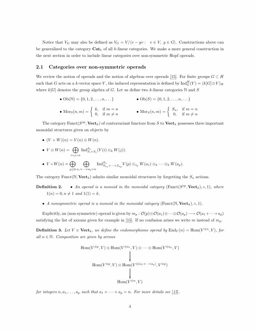
2.1 Categories over non-symmetric operads

We review the notion of operads and the notion of algebras over operads [15]. For finite groups G ⊂ H

such that G acts on a k-vector space V , the induced representation is defined by IndHG (V ) = (k[G]⊗V )H

where k[G] denotes the group algebra of G. Let us define two k-linear categories N and S

• Ob(N) = {0, 1, 2, . . . , n, . . . } • Ob(S) = {0, 1, 2, . . . , n, . . . }

• MorN(n, m) =

{k, if m = n0, if m 6= n

• MorS(n, m) =

{Sn, if m = n0, if m 6= n

The category Funct(Sop,Vectk) of contravariant functors from S to Vectk possesses three important

monoidal structures given on objects by

• (V + W )(n) = V (n) ⊕ W (n).

• V ⊗ W (n) =⊕

i+j=n

IndSn

Si×Sj(V (i) ⊗k W (j)).

• V ◦ W (n) =⊕

p≥0

⊕

a1+···+ap=n

IndSn

Sa1×···×SapV (p) ⊗sp

W (a1) ⊗k · · · ⊗k W (ap).

The category Funct(N,Vectk) admits similar monoidal structures by forgetting the Sn actions.

Definition 2. • An operad is a monoid in the monoidal category (Funct(Sop,Vectk), ◦, 1), where

1(n) = 0, n 6= 1 and 1(1) = k.

• A nonsymmetric operad is a monoid in the monoidal category (Funct(N,Vectk), ◦, 1).

Explicitly, an (non-symmetric) operad is given by mp : O(p)⊗O(a1)⊗· · ·⊗O(ap) −→ O(a1+· · ·+ap)

satisfying the list of axioms given for example in [15]. If no confusion arises we write m instead of mp.

Definition 3. Let V ∈ Vectk, we define the endomorphisms operad by EndV (n) = Hom(V ⊗n, V ), for

all n ∈ N. Composition are given by arrows

Hom(V ⊗p, V ) ⊗ Hom(V ⊗a1 , V ) ⊗ · · · ⊗ Hom(V ⊗ap , V )

��

Hom(V ⊗p, V ) ⊗ Hom(V ⊗(a1+···+ap), V ⊗p)

��Hom(V ⊗n, V )

for integers n, a1, . . . , ap such that a1 + · · · + ap = n. For more details see [15].

4

Let us introduce the category Pre-Catk of small pre-categories. Objects of Pre-Catk are called

small pre-categories. A small pre-category C consists of the following data:

• A set of objects Ob(C).

• A vector space MorC(x, y) associated to each pair of objects x, y ∈ Ob(C).

A morphisms F ∈ MorPre-Cat(C,D) from pre-category C to pre-category D consists of a map

F : Ob(C) −→ Ob(D) and a family of maps Fx,y : MorC(x, y) −→ MorD(F (x), F (y)), for x, y ∈ Ob(C).

Pre-Catk has a natural partial monoidal structure. Given pre-categories C and D such that

Ob(C) = Ob(D) = X , we define the product pre-category CD as follows

• Ob(CD) = X .

• MorCD(x, z) =⊕

y∈X MorC(x, y) ⊗ MorD(y, z).

The partial units are the pre-categories kX , defined as follows

• Ob(kX) = X .

• MorkX(a, b) =

{k, if a = b0, otherwise.

Given a pre-category C, we define the non-symmetric operad EndC(n) = MorPre-Cat(Cn, C), n ∈ N. We

used the convention C0 = kOb(C).

Definition 4. Let O be a non-symmetric k-linear operad. An O-category (C, γ) is a pre-category C

together with a non-symmetric operad morphism γ : O −→ EndC. Explicitly, a k-linear O-category C

consist of the following data:

• Objects Ob(C).

• Morphisms: HomC(x, y) ∈ Ob(Vectk), for each pair x, y ∈ Ob(C).

• For each, k ∈ N and objects x0, x1, . . . , xk ∈ Ob(C) maps

px0,...,xk: O(k) ⊗ HomC(x0, x1) ⊗ · · · ⊗ HomC(xk−1, xk) −→ HomC(x0, xk)

We usually write p instead of px0,...,xk.

These data should satisfy the following associativity axiom: Given objects x0, . . . , xn1+···+nk, and mor-

phisms ai ∈ HomC(xi−1, xi), i ∈ [n1 + · · · + nk], t ∈ O(k), ti ∈ O(ni), then

p(m(t; t1, . . . , tk); a1, . . . , an1+···+nk) =

p(t, p(t1; a1, . . . , an1), . . . , p(tk; an1+···+n(k−1)+1, . . . , an1+···+nk)).

5

For example if we are given objects xi ∈ Ob(C), for i = 0, 1, . . . , 5, morphisms ai ∈ Mor(xi−1, xi) for

i = 1, . . . , 5 and t ∈ O(5), then the morphism p(t; a1, . . . , a5) from object x0 to object x5 is represented

by the following diagram

-6

>-

~

?a1

a2

a3

a4

a5⇓t

p(t;a1,...,a5)

Given objects xi ∈ Ob(C), for i = 0, 1, . . . , 8, morphisms ai ∈ Mor(xi−1, xi), i = 1, 2, . . . , 8,

t1, t3 ∈ O(3), t2 ∈ O(2) and t ∈ O(4), then the axiom from Definition 4 is represented by the fol-

lowing commutative diagram.

?

-

I

±m(t;(t1,t2,t3))

⇓

:

7

w

?

-

z

W

=

p(t;p(t1;a1,a2,a3),p(t2;a4,a5),p(t3;a6,a7,a8))

a1

a4

a3

a5

a7

a6

a8

a2

-

I

±:

7

w z

W

=

tt1

t2

t3

a1

a4

a3

a5

a7

a6

-

a8

a2

-

p(t1;a1,a2,a3)

W

p(m(t;t1,t2,t3),a1,a2,...,a8)

t

⇓

º-

p(t2;a4,a5)

p(t3;a6,a7,a8)

-

⇒

⇓

⇐

Figure 1: Pictorial representation of the associative axiom of Definition 4.

Given a nonsymmetric operad O, we define the category OCatk as follows:

• Ob(OCatk) = small O-categories.

• Morphism MorO(C,D) from O-category C to O-category D are functors from C to D such that

F (p(t; a1, . . . , an)) = p(t; F (a1), . . . , F (an)),

for given objects x0, x1, . . . , xn, morphisms ai ∈ HomC(xi−1, x1), F (ai) ∈ HomD(F (xi−1); F (xi))

and t ∈ O(n). We call such a functor F an O-functor.

6

3 Polya Functors

Given an O-category C, Aut1(C) ⊂ FunctO(C, C) denotes the collection of invertible O-functors identical

on objects. Let G be a compact topological group. A G-action on an O-category C is a representation

ρ : G −→ Aut1(C). It is defined by a collection of actions ρx,y : G −→ GL(HomC(x, y)) such that

ρx0,xm(g)(p(t; a1, . . . , am)) = p(t; ρx0,x1(g)(a1), . . . , ρxn−1,xm

(g)(am))

for objects x0, x1, . . . , xn ∈ Ob(C), ai ∈ Hom(xi−1, xi), for all i ∈ [m] and g ∈ G. Abusing notation we

shall write ga instead of ρx,y(g)(a) where x, y ∈ Ob(C) and a ∈ Hom(x, y) . We define OCatk(G) to

be the category of all linear O-categories provided with G actions. Morphisms F from O-category C to

O-category D are G-equivariant O-functors F from C into D, i.e., F (ga) = gF (a), for all a ∈ Mor(x, y),

g ∈ G, where x, y ∈ Ob(C). We define

Inv : OCatk(G) −→ OCatk

C 7−→ CG

as follows: Ob(CG) = Ob(C) , MorCG(x, y) = MorC(x, y)G. CG is a O-category since

gp(t; a1, . . . , am) = p(t; ga1, . . . , gam) = p(t; a1, . . . , am).

We defineCoinv : OCatk(G) −→ OCatk

C 7−→ CG

as follows: Ob(CG) = Ob(C), MorCG(x, y) = MorC(x, y)G and

p(t; a1, a2, . . . , am) =1

vol(G)m−1

∫

G(n−1)

p(t; a1, g2a2, g3a3, . . . , gmam)dg2dg3 . . . dgm (1)

Theorem 5. There is a natural isomorphism s : Coinv −→ Inv i.e., for C ∈ Ob(OCatk(G)) we are

given an isomorphism sC : Coinv(C) −→ Inv(C) such that Inv(F ) ◦ sC = sD ◦ Coinv(F ), for all functors

F : C −→ D in the category OCatk(G).

Proof. Given a category C and objects x, y ∈ Ob(C), let sx,y : HomC(x, y) −→ HomC(x, y)G the sym-

metrization map defined in the Section 2. By Proposition 1, it induces an isomorphism of vector spaces

sx,y : HomC(x, y)G −→ HomC(x, y)G.

It remains to check that the following diagram is commutative

O(k) ⊗ HomC(x0, x1)G ⊗ · · · ⊗ HomC(xm−1, xm)G

id⊗s

++WWWWWWWWWWWWWWWWWWWWWW

p(t,−)

ssgggggggggggggggggggggg

HomC(x0, xm)G

sx0,xm++WWWWWWWWWWWWWWWWWWWWWW

O(k) ⊗ HomC(x0, x1)G ⊗ · · · ⊗ HomC(xm−1, xm)G

p(t,−)ssggggggggggggggggggggg

HomC(x0, xm)G

7

where s = sx0,x1 ⊗ · · · ⊗ sxm−1,xm. Clearly,

p(t;−)id ⊗ S =1

vol(G)m

∫

Gm

p(t; g1a1, . . . , gmam)dg1dg2 . . .dgm.

On the other hand,

sx0,xmp(t; a1, . . . , am) =

1

vol(G)

∫

G

g1p(t; a1, . . . , am)dg1

=1

vol(G)m

∫

Gm

g1p(t; a1, h2a2, . . . , hmam)dg1dh2 . . . dhm

=1

vol(G)m

∫

Gm

p(t; g1a1, g1h2a2, . . . , g1hmam)dg1dh2 . . . dhm

=1

vol(G)m

∫

Gm

p(t; g1a1, . . . , gmam)dg1dg2 . . . dgm

making the change of variables g2 = g1h2, . . . , gm = g1hm.

Notice that if O is an operad then O ⊗O is naturally an operad with (O ⊗O)(n) = O(n) ⊗O(n).

Definition 6. A Hopf operad is an operad together with an operad morphism ∆ : O −→ O ⊗O.

We have the following lemma

Lemma 7. If O is a Hopf operad then the category of O-algebras is monoidal.

Proof. If A and B are O-algebras then A ⊗ B is also an O-algebra, as the following diagram shows

O(n) ⊗ (A ⊗ B)⊗n −→ (O(n) ⊗ A⊗n) ⊗ (O(n) ⊗ B⊗n) −→ A ⊗ B.

We now construct a partial monoidal structure on OCat.

Definition 8. Let O be a Hopf operad, given O-categories C and D such that Ob(C) = Ob(D) = X, we

define the tensor product category C ⊗ D as follows

• Ob(C ⊗ D) = X.

• MorC⊗D(x, y) = MorC(x, y) ⊗ MorD(x, y).

• p(t; a1⊗b1, . . . , an⊗bn) =∑

p(t(1); a1, . . . , an)⊗p(t(2); b1, . . . , bn), where ∆(t) =∑

t(1)⊗t(2) using

Swedler notation.

Recall the well-known definition. Given a pair of groups G and K ⊂ Sn the semidirect product

Gn⋊K is the set Gn

⋊K = {(g, a) : g ∈ Gn, a ∈ K} provided with the product (g, a)(h, b) = (ga(h), ab)

where g, h ∈ Gn, a, b ∈ K and if h = (h1, . . . , hn) then a(h1, . . . , hn) = (ha−1(1), . . . , ha−1(n)). The

following result is obvious

8

Lemma 9. a. Ob(C⊗n) = Ob(C), MorC⊗n(x, y) = MorC(x, y)⊗n.

b. If G acts on C and K ⊂ Sn then Gn ⋊ K acts on C⊗n.

Assume that C is a category over a non-symmetric Hopf operad O. Let G be a compact topological

group, and K a subgroup of Sn. We construct functor PG,K which we call the Polya functor of type

G, K

PG,K : OCatk(G) −→ OCatk

as follows:

• On objects: Given C ∈ Ob(OCatk(G)), then PG,K(C) ∈ Ob(OCatk) is the category

PG,K(C) = C⊗n/Gn⋊ K.

Explicitly:

• Ob(PG,K(C)) = Ob(C⊗n) = Ob(C), and for given objects x, y ∈ Ob(PG,K(C)),

MorPG,K(C)(x, y) = (MorC(x, y)⊗n)/Gn⋊ K.

• Identity: idx ∈ MorPG,K(C)(x, x) = id⊗nx ∈ (MorC(x, x)⊗n)/Gn

⋊ K.

• Composition: Given x0, . . . , xm ∈ Ob(PG,K(C)) and morphisms ai ∈ MorPG,K(C)(xi−1, xi), for

i = 1, . . . , m, we have the following

p(t; a1, . . . , am) =1

((♯(G)n)♯(K))m−1

∑

(g,s)∈(Gn⋊K)m−1

p(t; a1, (g2, s2)a2, . . . , (gm, sm)am) if G is finite,

p(t; a1, . . . , am) =1

(vol(Gn)♯(K))m−1

∑

s∈Km−1

∫

g∈(Gn)m−1

p(t; a1, (g2, s2)a2, . . . , (gm, sm)am)dg2 . . .dgm,

if G is compact and gi ∈ Gn.

• On morphisms: each functor Cα //D induces a functor C⊗n α⊗n

//D⊗n . This functor descends

to a well defined functor

PG,K(C) = C⊗n/Gn ⋊ K //D⊗n/Gn ⋊ K = PG,K(D) .

Example 10. Consider the non-symmetric operad ASS given by ASS(n) = k, for all n ≥ 0. ASS-

categories are categories in the usual sense. This example will be applied in Section 4 to introduce explicit

formulae for the composition of morphisms in the Schur categories of various types.

Definition 11. Let O be an operad. An O-algebra is a pair (A, γ) where A is a vector space and

γ : O −→ EndA is an operad morphism.

9

Notice that an O-algebra may be regarded as an O-category C with one object by setting A =

MorC(1, 1). We denote by OAlgk the category of O-algebras and by OAlgk(G) the category of O-

algebras provided with a G action. We have two naturally isomorphic functors

Inv : OAlgk(G) −→ OAlgk

A 7−→ AG

Coinv : OAlgk(G) −→ OAlgk

A 7−→ AG

Let O be a Hopf operad. Assume that A is an O-algebra. Let G be a compact topological group and

K ⊂ Sn. We have a functor

PG,K : OAlgk(G) −→ OAlgk

A 7−→ A⊗n/Gn ⋊ K

The O-algebra structure on A⊗n/Gn ⋊ K is given for any a1, . . . , am ∈ A, t ∈ O(m) by

p(t; a1, . . . , am) =1

((♯(G)n)♯(K))m−1

∑

(g,s)∈(Gn⋊K)m−1

p(t; a1, (g2, s2)a2, . . . , (gm, sm)am) (2)

if G is finite. If G is compact taking gi ∈ Gn we have that

p(t; a1, . . . , am) =1

(vol(Gn)♯(K))m−1

∑

s∈Km−1

∫

g∈(Gn)m−1

p(t; a1, (g2, s2)a2, . . . , (gm, sm)am)dg2 . . . dgm.

Corollary 12. Let A be an O-algebra, G a finite group acting by algebra automorphism on A. Take

K = {id}. The following identity hold in PG(A)

a b =1

♯(G)

∑

g∈G

a(gb) (3)

where a, b ∈ A.

We remark that Joyal theory of analytic functors, see [12], [13], may be extended from the context of

k-vector spaces to O-algebras by defining a functor F which sends a family A = {An}n≥0 of O-algebras

provided with right Sn actions, into the functor FA from the OAlg into OAlg given as follows

F : Funct(Sop,OAlg) −→ Funct(OAlg,OAlg)

A = {An}n≥0 7−→ FA(B) =⊕

n≥0

(An ⊗ B⊗n)Snfor all B ∈ Ob(OAlg)

Example 13. Consider the operad Ass given by Ass(n) = k[Sn], for n ≥ 0. Ass-algebras are the same

as associative algebras. If we take the family k = {k}n, n ≥ 0, provided with the trivial Sn action, then

Fk(A) = Sym(A)

The following remarks justify our choice of name for the Polya functors. Let K ⊂ Sn be a permutation

group. For k ∈ K, let bs(k) be the number of cycles of k of length s. The cycle index polynomial of

K ⊂ Sn, is the polynomial in n variables x1, . . . , xn

PK(x1, . . . , xn) =1

♯(K)

∑

k∈K

xb1(k)1 x

b2(k)2 . . . xbn(k)

n .

10

Let A be a finite dimensional O-algebra and X a basis for A. Using Polya theory [22], we can compute

the dimension of the O-algebra (A⊗n)K as follows:

dim((A⊗n)K) = ♯(Xn/K)

= PK(♯(X), ♯(X), . . . , ♯(X))

= PK(dim A, dimA, . . . , dimA).

3.1 General multiplication rule

For each K ⊂ Sn consider the Polya functor PK : k-alg −→ k-alg from the category of associative

k-algebras into itself defined on objects as follows: if A is a k-algebra, then PK(A) denotes the algebra

whose underlying vector space is

PK(A) = (A⊗n)/〈a1 ⊗ · · · ⊗ an − aσ−1(1) ⊗ · · · ⊗ aσ−1(n) : ai ∈ A, σ ∈ K〉.

Our next theorem provides the rule for the product of m elements in PK(A).

Theorem 14. For any aij ∈ A the following identities holds in PK(A)

♯(K)m−1m∏

i=1

n⊗

j=1

aij

=∑

σ∈{id}×Km−1

n⊗

j=1

(m∏

i=1

aiσ−1i

(j)

)(4)

Proof. It is follows from formula (2), taking Ass as the underlying operad and setting G = {id}.

Theorem 14 implies the following

Proposition 15. Let A be an algebra provided with a basis {es|s ∈ [r]}. Assume that eset = c(k, s, t)ek

(sum over k), for all s, t ∈ [r]. For any given a = (aij) ∈ Mn×m([r]) the following identity holds in

PK(A)

(n!)m−1m∏

i=1

n⊗

j=1

eaij

=∑

σ,α

n∏

j=1

c(αj , a, σ)

n⊗

j=1

eα

jm−1

,

where the sum runs over all σ ∈ {id} × Km−1, α = (αji ) ∈ M(m−1)×n([r]), and

c(αj , a, σ) = c(αj1, a1σ

−11 (j), a2σ

−12 (j))c(α

j2, α

j1, a3σ

−13 (j)) . . . c(αj

m−1, αjm−2, amσ

−1m (j)).

Proof.

(n!)m−1m∏

i=1

n⊗

j=1

eaij

=∑

σ∈{id}×Gm−1

n⊗

j=1

(m∏

i=1

eaiσ

−1i

(j)

)

=∑

α,σ

n⊗

j=1

c(α, a, σ)eαm−1

=∑

σ,α

n∏

j=1

c(αj , a, σ)

n⊗

j=1

eα

jm−1

11

Let us consider a non-symmetric Hopf operad O. Assume that a basis ptm, t ∈ [km], for O(m) is

given for each m ∈ N. Moreover let us assume that ∆(ptm) = pt

m ⊗ · · · ⊗ ptm, then the next proposition

follows from formula (4).

Proposition 16. Let A be an O-algebra provided with a basis {es|s ∈ [r]}, and let O(n) = 〈ptm : t ∈

[rm]〉. Assume that ptm(es1 , . . . , esm

) = c(t, k, m, s1, . . . , sn)ek, (sum over k). For any given a = (aij) ∈

Mn×m([r]), the following identity holds in PK(A)

ptm(⊗n

j=1ea1j, . . . ,⊗n

j=1eamj) =

∑

σ,u

n∏

j=1

c(t, uj , m, a1σ−11 (j), . . . , amσ

−1m (j))

n⊗

j=1

euj

where the sum runs over all σ ∈ {id} × Km−1 and u ∈ [r]n.

4 Symmetric power of a supercategory.

Let us consider Polya functor PG,K : Catk(G) −→ Catk for the case G = id, K = Sn, i.e, we consider

for each n ∈ N the functor

Symn : Catk −→ Catk

Recall that a supercategory is a category over the category Supervect of Z2-graded vector spaces with

the Koszul rule of signs. Functor Symn may be applied to supercategories as well. The next result

provides formula for the composition of morphisms in the symmetric powers of a supercategory. We use

the notation a1 . . . an = a1 ⊗ · · · ⊗ an ∈ Symn(HomC(x, y)), for morphisms a1, . . . , an ∈ HomC(x, y).

Proposition 17. Let C be a supercategory and let a1, . . . , an ∈ MorC(x, y) and b1, . . . , bn ∈ MorC(y, z).

In the supercategory Symn(C) the compositions of morphisms is given by

(a1a2 . . . an)(b1b2 . . . bn) =1

n!

∑

σ∈Sn

sgn(a, b, σ)(a1bσ−1(1))(a2bσ−1(2)) . . . (anbσ−1(n))

where sgn(a, b, σ) = (−1)e and e = e(a, b, σ) =∑

i>j aibσ−1(j) +∑

σ(i)>σ(j) bibj .

4.1 Schur categories

Let k be a field of characteristic 0, m = (m1, . . . , mk) ∈ Nk, Zm = Zm1 × · · · × Zmkand n ∈ N. We

define the Schur supercategory of type (m, n) as follows:

Ob(S(m, n)) = finite dimesional k-supervector spaces.

MorS(m,n)(V, W ) = (Homk(V ⊕Zm , W⊕Zm)⊗n)Znm⋊Sn

.

Znm ⋊ Sn acts on (Homk(V ⊕Zm , W⊕Zm)⊗n) as follows

Znm ⋊ Sn × (Homk(V ⊕Zm , W⊕Zm)⊗n) −→ (Homk(V ⊕Zm , W⊕Zm)⊗n)

((c1, . . . , cn), σ)(Et1u1r1s1

. . . Etnunrnsn

) 7−→ (Etσ(1)(u1+c1)

rσ(1)(s1+c1). . . E

tσ(n)(un+cn)

rσ(n)(sn+cn) )

12

where E(V, W )klij are the elementary linear transformation in (Homk(V ⊕Zm , W⊕Zm), i ∈ [dim V ],

k ∈ [dim W ] and j, l ∈ Zkm. We apply Polya functor to obtain explicit formula for the composition rule

Mor(V, W ) ⊗ Mor(W, Z) −→ Mor(V, Z).

Theorem 18. For any given M = m1 . . . mk, i, t ∈ [dimW ], k ∈ [dim Z], r ∈ [dimV ], and j, l, s, u ∈

Znm, we have

(E(V, W )k1l1i1j1

. . . E(V, W )knlninjn

)(E(W, Z)t1u1r1s1

. . . E(W, Z)tnunrnsn

) =

1

Mnn!

∑

σ ∈ Sn

tσ(a) = ia

sgn(σ, i, k, r, t)E(V, Z)k1l1rσ(1)(s1+j1−u1)

. . . E(V, Z)knlnrσ(n)(sn+jn−un)

where sgn(σ, i, k, r, t) = (−1)e and

e =∑

i>j

(ii + ki)(rσ−1(i) + tσ−1(i)) +∑

σ(i)>σ(j)

(rσ−1(i) + tσ−1(i))(rσ−1(j) + tσ−1(j)).

Proof. Straightforward using Polya functor and Proposition 17.

We now develop a graphical notation that make transparent the meaning of Theorem 18. Let us

assume that n = 4, k = 4, m1 = 6, m2 = 3, dim(V ) = 4, dim(W ) = 2 and dim(Z) = 3. We represent an

elementary linear transformation E(V, W ) as in Figure 2

7−→E(V,W )klij

3

6

3

Figure 2: Representation of elementary transformation.

Notice that each block corresponds to Z6 ×Z3, Z6 acting horizontally, and Z3 acting vertically. The

number of blocks in the bottom row is dim(V ), and the number of blocks in the top row is dim(W ). El-

ements of (Hom(V ⊕Zm , W⊕Zm)⊗n)(Z6×Z3)4⋊S4are depicted by four non-numbered arrows, and similarly

for elements of (Hom(W⊕Zm , Z⊕Zm)⊗n)(Z6×Z3)4⋊S4. Composition is obtained as follows

• Fix an arbitrary enumeration of the arrows in (Hom(V ⊕Zm , W⊕Zm)⊗n)(Z6×Z3)4⋊S4.

• Sum over all possible enumerations of the arrows in (Hom(W⊕Zm , Z⊕Zm)⊗n)(Z6×Z3)4⋊S4.

• Stacks arrows from (Hom(V ⊕Zm , W⊕Zm)⊗n)(Z6×Z3)4⋊S4to arrows on (Hom(W⊕Zm , Z⊕Zm)⊗n)(Z6×Z3)4⋊S4

taking care of enumeration and using the Z2 × Z6 symmetry.

Notice that composition is interesting in that no-touching arrows may nevertheless be composed (due

to the Z6 × Z3 symmetry) as shown in Figure 3.

13

* 3} k

�1

o]

1

�

2

2

3

3

4

4

=

1

k

2

}

4

>

3

>

Figure 3: Example of composition.

Definition 19. The Schur superalgebra of type (sdimV, m) is given by HomSn(V ⊗n, V ⊗n), where sdim

denotes the superdimension of a supervector space.

See [10] for more on Schur algebras.

Corollary 20. For m = 1 and V = W , MorS(m,n)(V, V ) is the Schur superalgebra Schur(sdimV, m) of

type (sdimV, m).

Proof. (Hom(V, V )⊗n)Sn∼= (Hom(V, V )⊗n)Sn ∼= HomSn

(V ⊗n, V ⊗n).

5 Classical symmetric functions

In this section we study classical symmetric functions by means of the Polya functor. We provide a fairly

elementary interpretation of the symmetric functions in terms of the symmetric powers of the monoidal

algebra associated to the additive monoid Nm. We also consider symmetric odd-functions as well as

symmetric Boolean algebras. Symmetric functions have been studied from many points of view, see for

example [16], [19], [21] .

5.1 Symmetric functions of Weyl type

The classical Weyl groups of type An, Bn, and Dn, are Sn, Zn2 ⋊ Sn and Z

n−12 ⋊ Sn respectively. These

groups act on (Rm)n as follows:

Sn × (Rm)n −→ (Rm)n

(σ, (x1, . . . , xn)) 7−→ (xσ−1(1), . . . , xσ−1(n))

(Zn2 ⋊ Sn) × (Rm)n −→ (Rm)n

((t1, . . . , tn), σ)(x1, . . . , xn) 7−→ (t1xσ−1(1), . . . , tnxσ−1(n))

The group Dn is regarded as a subgroup of Bn as follows

Zn−12 ⋊ Sn = {((t1, . . . , tn), σ) ∈ Z

n2 ⋊ Sn : t1t2 . . . tn = 1}.

Definition 21. Fix m ∈ N. The algebra of symmetric functions of type An, Bn and Dn are given by

• SymAn(m) = (C[x1, . . . , xn])Sn

∼= (C[x1, . . . , xn])Sn ,

• SymBn(m) = (C[x1, . . . , xn])Zn

2 ⋊Sn∼= (C[x1, . . . , xn])Z

n2 ⋊Sn,

14

• SymDn(m) = (C[x1, . . . , xn])

Zn−12 ⋊Sn

∼= (C[x1, . . . , xn])Zn−12 ⋊Sn,

where xi = (xi1, . . . , xim), for i = 1, . . . , n.

The map C[Nm]⊗n −→ C[x1, . . . , xn] given by a1 ⊗ · · · ⊗ an 7−→ xa11 . . . xan

n defines an isomorphism

of algebras, where ai ∈ Nm and xai

i = xai1

i1 . . . xaim

im . We set Nme = {a ∈ Nm : |a| is even} and

Nmo = {a ∈ Nm : |a| is odd}. We denote XA = xa1

1 . . . xann , for A = (a1, . . . , an) ∈ (Nm)n.

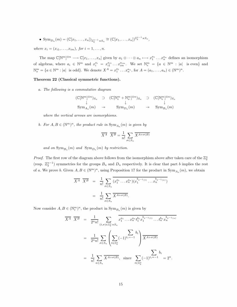
Theorem 22 (Classical symmetric functions).

a. The following is a commutative diagram

(C[Nm]⊗n)Sn⊃ (C[Nm

e + Nmo ]⊗n)Sn

⊃ (C[Nme ]⊗n)Sn

↓ ↓ ↓SymAn

(m) ։ SymDn(m) ։ SymBn

(m)

where the vertical arrows are isomorphisms.

b. For A, B ∈ (Nm)n, the product rule in SymAn(m) is given by

XA XB =1

n!

∑

σ∈Sn

XA+σ(B)

and on SymBn(m) and SymDn

(m) by restriction.

Proof. The first row of the diagram above follows from the isomorphism above after taken care of the Zn2

(resp. Zn−12 ) symmetries for the groups Bn and Dn respectively. It is clear that part b implies the rest

of a. We prove b. Given A, B ∈ (Nm)n, using Proposition 17 for the product in SymAn(m), we obtain

XA XB =1

n!

∑

σ∈Sn

(xa11 . . . xan

n )(xb

σ−1(1)

1 . . . xb

σ−1(n)n )

=1

n!

∑

σ∈Sn

XA+σ(B).

Now consider A, B ∈ (Nme )n, the product in SymBn

(m) is given by

XA XB =1

2nn!

∑

(t,σ)∈Zn2 ⋊Sn

xa11 . . . xan

n tb11 xb

σ−1(1)

1 . . . tbnn x

bσ−1(n)

n

=1

2nn!

∑

σ∈Sn

∑

t∈Zn2

(−1)

∑

ti=−1

bi

XA+σ(B)

=1

n!

∑

π∈Sn

XA+σ(B), since∑

t∈Zn2

(−1)

∑

ti=−1

bi

= 2n.

15

Consider A, B ∈ (Nne + Nm

o )n, we obtain

XA XB =1

2n−1n!

∑

(t,σ)∈Zn2 ⋊Sn

xa11 . . . xan

n tb11 xb

σ−1(1)

1 . . . tbnn x

bσ−1(n)

n

=1

2n−1n!

∑

π∈Sn

∑

t∈Zn2∏

ti=1

(−1)

∑

ti=−1

bi + bn

XA+σ(B)

=1

n!

∑

σ∈Sn

XA+σ(B), since∑

t∈Zn2∏

ti=1

(−1)

∑

ti=−1

bi + bn

= 2n−1

5.2 Symmetric odd-functions

Consider the alternating algebra∧

[θ1, . . . , θm], which we regard as the algebra of functions on the purely

odd super-space R0|m. A basis for∧

[θ1, . . . , θm] is given by {θI = θi1 . . . θik| I ⊂ [m]}. The structural

coefficients are given by θIθJ = c(I, J)θI∪J , where c(I, J) = (−1)|{i∈I,j∈J, i>j}|, if I ∩ J = ∅, and 0

otherwise. The algebra∧

[θ1, . . . , θm] is Z2-graded, with grading θI = I = 0 if |I| is even and θI = I = 1

if |I| is odd. Now we apply Polya functor to obtain

Proposition 23. The product rule in the algebra of symmetric odd functions (∧

[θ1, . . . , θm]⊗n)Snis

given by

(θI1 . . . θIn)(θJ1 . . . θJn

) =1

n!

∑

σ∈Sn

(sgn(I, J, σ)

n∏

k=1

c(Ik, Jσ−1(k))

)n∏

i=1

θIk∪Jσ−1(k)

,

where sgn(I, J, σ) = (−1)e and e =∑

k>l

IkJσ−1(l) +∑

σ(k)>σ(l)

JkJl.

Proof.

(θI1 . . . θIn)(θJ1 . . . θJn

) =1

n!

∑

σ∈Sn

sgn(I, J, σ)(θI1θJσ−1(1)

) . . . (θInθJ

σ−1(n))

=1

n!

∑

σ∈Sn

sgn(I, J, σ)

(n∏

k=1

c(Ik, Jσ−1(k))θIk∪Jσ−1(k)

)

=1

n!

∑

σ∈Sn

(sgn(I, J, σ)

n∏

k=1

c(Ik, Jσ−1(k))

)n∏

k=1

θIk∪Jσ−1(k)

16

5.3 Symmetric Boolean algebra

Fix n ∈ N and let P (n) be the free C-vector space generated by the subsets of [n], i.e., P (n) = 〈A : A ⊂

[n]〉. Define a product ∪ on P (n) by

∪ : P (n) ⊗ P (n) −→ P (n)A ⊗ B 7−→ A ∪ B

(P (n),∪) is a Boolean algebra and dim(P (n)) = 2n. Sn acts naturally on [n] and thus on P (n). We call

the algebra (P (n),∪)/Sn∼= (P (1)⊗n)/Sn = Symn(P (1)) the symmetric Boolean algebra; it has dimension

n + 1, a basis being {[0], [1], . . . , [n]}. We define P (n, k) := {A ⊂ [n] : |A| = k}. An application of Polya

functor yields the next

Theorem 24. [a][b] =1(nb

)m∑

k=0

(a

b − k

)(n − a

k

)[a + k], for all [a], [b] ∈ (P (n),∪)Sn

, and

m = min(b, n − a).

Proof.

[a][b] =1

n!

∑

σ∈Sn

[a] ∪ σ[b] =1(nb

)∑

B∈P [n,b]

[a] ∪ B

=1(nb

)∑

B0⊂P ([n]−[a],k)

B1⊂P ([a],b−k)

[a] ∪ B0 =1(nb

)m∑

k=0

(a

b − k

)(n − a

k

)[a + k]

6 Quantum symmetric functions

In this section we assume the reader is familiar with the notations from [14]. Let us recall the notion of

a formal deformation

Definition 25. Fix a Poisson manifold (M, {, }). A formal deformation (deformation quantization) of

the algebra of smooth functions on M is an associative star product

⋆ : C∞(M)[[~]] ⊗R[[~]] C∞(M)[[~]] −→ C∞(M)[[~]] such that:

a. f ⋆ g =

∞∑

n=0

Bn(f, g)~n, where Bn(−,−) are bi-differential operators .

b. f ⋆ g = fg + 12{f, g}~ + O(~2), where O(~2) are terms of order ~2.

In [14] a canonical ⋆-product has been constructed for any Poisson manifold. For manifold (Rm, α)

with Poisson bivector α, the ⋆-product is given by the formula

f ⋆ g =

∞∑

n=0

~n

n!

∑

Γ∈Gn

ωΓBΓ,α(f, g),

17

where Gn is a collection of admissible graphs each of which has n edges, and ωΓ are some constants (in-

dependent of the Poisson manifold). Given a finite group K acting on (C∞(M), ⋆) by algebra automor-

phisms, we call the algebra (C∞(M)[[~]], ⋆)K∼= (C∞(M)[[~]], ⋆)K the algebra of quantum K-symmetric

functions on M .

Next theorem shows how groups of automorphisms of (C∞(M)[[~]], ⋆) arise in a natural way.

Theorem 26. Assume we are given a Poisson structure {-, -} on Rm, and a group K ⊂ Sm such that

{-, -} is K-equivariant. Then K acts on (C∞(Rm)[[~]], ⋆) by automorphisms.

Proof. We assume that {f, g} ◦ σ = {f ◦ σ, g ◦ σ}, for all f, g ∈ C∞(Rm), σ ∈ K, or equivalently

αij(σx) = ασ(i)σ(j) , where αij = {xi, xj} for all i, j ∈ [m]. Let us show that σ(f ⋆ g) = (σf) ⋆ (σg).

σ(f ⋆ g)(x) = (f ⋆ g)(σ−1x) =

∞∑

n=0

~n

n!

∑

Γ

wΓBΓ,α(f, g)(σ−1x).

On the other hand

(σf) ⋆ (σg)(x) =∞∑

n=0

~n

n!

∑

Γ

wΓBΓ,α(σf, σg)(x).

We need to prove that

BΓ,α(f, g)(σ−1x) = BΓ,α(σf, σg)(x), for all Γ ∈ Gn.

Using Kontsevich’s formula (see [14]) we get

BΓ,α(f, g)(σ−1x) =∑

I:EΓ−→[m]

n∏

i=1

∏

e∈EΓ,e=(∗,i)

∂I(e)

αI(e1i )I(e2

i )

(σ−1x)×

∏

e∈EΓ,e=(∗,L)

∂I(e)

f

(σ−1x) ×

∏

e∈EΓ,e=(∗,R)

∂I(e)

g

(σ−1x)

=∑

I:EΓ−→[m]

n∏

i=1

∏

e∈EΓ,e=(∗,i)

∂σ(I(e))

ασ(I(e1i ))σ(I(e2

i ))

(x)×

∏

e∈EΓ,e=(∗,L)

∂σ(I(e))

f ◦ σ−1

(x) ×

∏

e∈EΓ,e=(∗,R)

∂σ(I(e))

g ◦ σ−1

(x)

= BΓ,α(σf, σg)(x).

Corollary 27. Under the conditions above, the product rule on (C∞((Rm)n)[[~]], ⋆)K is given by

f ⋆ g =∑

σ∈K

∞∑

n=0

~n

n!

(∑

Γ

wΓBΓ,α(f, g ◦ σ−1)

)(5)

for all f, g ∈ C∞(Rm)n[[~]].

18

Proof. Using Polya functor corollary 12, we have

f ⋆ g =∑

σ∈K

f ⋆ σg =∑

σ∈K

∞∑

n=0

~n

n!

(∑

Γ

wΓBΓ,α(f, g ◦ σ−1)

).

Definition 28. Given a Poisson manifold (Rm, { , }) and a subgroup K ⊂ Sn the algebra of quantum

symmetric functions on (Rm)n is set to be (C∞(Rm)n[[~]], ⋆)K∼= (C∞(Rm)n[[~]], ⋆)K .

Notice that if (Rm, α) is a Poisson manifold then (Rm)n is a Poisson manifold in a natural way.

Moreover the Poisson structure on (Rm)n is Sn-equivariant, and thus K-equivariant for all subgroup K

of Sn.

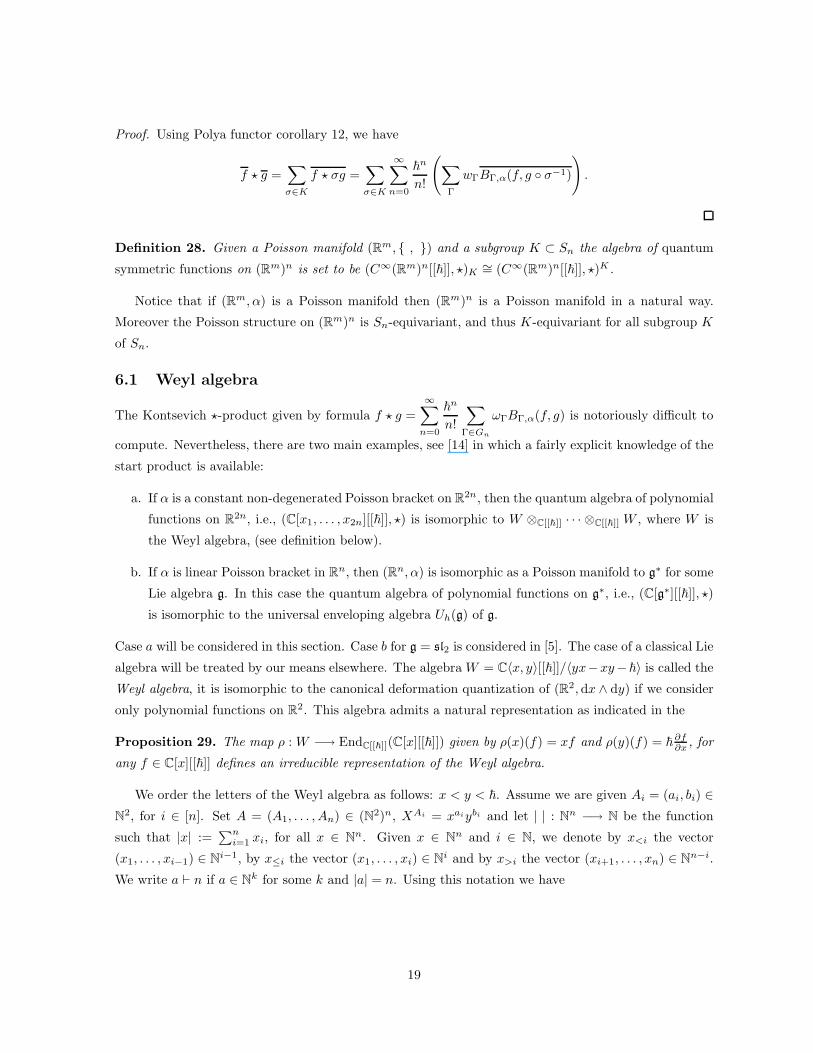
6.1 Weyl algebra

The Kontsevich ⋆-product given by formula f ⋆ g =

∞∑

n=0

~n

n!

∑

Γ∈Gn

ωΓBΓ,α(f, g) is notoriously difficult to

compute. Nevertheless, there are two main examples, see [14] in which a fairly explicit knowledge of the

start product is available:

a. If α is a constant non-degenerated Poisson bracket on R2n, then the quantum algebra of polynomial

functions on R2n, i.e., (C[x1, . . . , x2n][[~]], ⋆) is isomorphic to W ⊗C[[~]] · · · ⊗C[[~]] W , where W is

the Weyl algebra, (see definition below).

b. If α is linear Poisson bracket in Rn, then (Rn, α) is isomorphic as a Poisson manifold to g∗ for some

Lie algebra g. In this case the quantum algebra of polynomial functions on g∗, i.e., (C[g∗][[~]], ⋆)

is isomorphic to the universal enveloping algebra Uh(g) of g.

Case a will be considered in this section. Case b for g = sl2 is considered in [5]. The case of a classical Lie

algebra will be treated by our means elsewhere. The algebra W = C〈x, y〉[[~]]/〈yx−xy−~〉 is called the

Weyl algebra, it is isomorphic to the canonical deformation quantization of (R2, dx ∧ dy) if we consider

only polynomial functions on R2. This algebra admits a natural representation as indicated in the

Proposition 29. The map ρ : W −→ EndC[[~]](C[x][[~]]) given by ρ(x)(f) = xf and ρ(y)(f) = ~∂f∂x

, for

any f ∈ C[x][[~]] defines an irreducible representation of the Weyl algebra.

We order the letters of the Weyl algebra as follows: x < y < ~. Assume we are given Ai = (ai, bi) ∈

N2, for i ∈ [n]. Set A = (A1, . . . , An) ∈ (N2)n, XAi = xaiybi and let | | : Nn −→ N be the function

such that |x| :=∑n

i=1 xi, for all x ∈ Nn. Given x ∈ Nn and i ∈ N, we denote by x<i the vector

(x1, . . . , xi−1) ∈ Ni−1, by x≤i the vector (x1, . . . , xi) ∈ Ni and by x>i the vector (xi+1, . . . , xn) ∈ Nn−i.

We write a ⊢ n if a ∈ Nk for some k and |a| = n. Using this notation we have

19

Definition 30. The normal coordinates N(A, k) ofn∏

i=1

XAi ∈ W are defined through the identity

n∏

i=1

XAi =

min∑

k=0

N(A, k)x|a|−ky|b|−k~

k (6)

for 0 ≤ k ≤ min = min(|a|, |b|). For k > min, we set N(A, k) equal to 0.

Recall that given finite sets N and M with n and m elements respectively, the number of one-to-one

functions f : N −→ M is m(m− 1) . . . (m− n + 1) = (m)n. The number (m)n is called the n-th falling

factorial of m. The n-th rising factorial m(n) of m is given by m(n) = m(m +1) . . . (m +n− 1). For any

a, b ∈ Nn, we define(ab

):=(a1

b1

)(a2

b2

). . .(an

bn

), and a! = a1!a2! . . . an!.

Definition 31. A k-pairing from set E to set F is an injective function from a k-elements subset of E

to F . We denote by Pk(E, F ) the set of k-pairings from E to F .

Definition 32. Fix variables t = (t1, . . . , tn) and s = (s1, . . . , sn). The generating series N of the

normal coordinates in the Weyl algebra is given by

N =∑

a,b,c

N(A, c)sa

a!

tb

b!uc ∈ C[[s, t, u]] (7)

where the sum runs over a, b ∈ Nn, c ∈ N and A = (A1, . . . , An) ∈ (N2)n.

Theorem 33. Let A, k be as in the Definition 30, the following identity holds

a. N(A, k) =∑

p⊢k

(b

p

) n−1∏

i=1

(|a>i| − |p>i|)pi, where p ∈ Nn−1.

b. Let E1, . . . , En, F1, . . . , Fn be disjoint sets such that ♯(Ei) = ai, ♯(Fi) = bi, for i ∈ [n], set E =

∪ni=1Ei, and F = ∪n

i=1Fi, then N(A, k) = ♯({p ∈ Pk(E, F ) | if (a, p(a)) ∈ Ei × Fj then i > j}).

c. N = exp

∑

i>j

utisj +∑

i

ti +∑

j

sj

.

Proof. Using induction one show that the following identity hold in the Weyl algebra

ybxa =

min∑

k=0

(b

k

)(a)kxa−kyb−k

~k, (8)

where min = min(a, b) . Several applications of identity (8) imply a. Notice that for given sets E, F

such that ♯(E) = a and ♯(F ) = b,(

bk

)(a)k is equal to ♯({p ∈ Pk(E, F )}), showing part b for n = 2. The

general formula follows from induction. This prove b. It follows from standard combinatorial facts (see

[20], [22] for more details) that

exp

∑

i>j

utisj +∑

i

ti +∑

j

sj

=∑

a,b,c

ca,b,c

sa

a!

tb

b!

uc

c!

where ca,b,c = ♯({(p, σ) : p ∈ Pc(A, B) and σ : [c] → p, a bijection }) which is equivalent to formula

(7).

20

Figure 4 illustrates the combinatorial interpretation of the normal coordinate N(A, k) of an element3∏

i=1

XAi ∈ W , it shows are of the possible pairing contributing to N(A, k).

E1F1 E2 F2 E3 F3

Figure 4: Combinatorial interpretation of N.

Corollary 34. For any given (t, a, b) ∈ N × Nn × Nn, the following identity holds

n∏

i=1

(t + |a>i| − |b>i|)bi=∑

p⊢k

(b

p

) n−1∏

i=1

(|a>i| − |p>i|)pit|b|−k

Proof. Consider the identity (6) in the representation of the Weyl algebra defined in Proposition 29.

Apply both sides of the identity (6) to xt for t ∈ N and use Theorem 33.

Theorem 35. Let A, c be as in the Definition 30. The following identity holds

N(A, c) =∑

∑cij=c

k∏

j=2

(aj∑i cij

)( ∑i cij

cij . . . c(j−1)j

) k−1∏

i=1

(bi∑j cij

)( ∑j cij

ci(i+1) . . . cik

)∏

i>j

cij !

where cij are integers with 1 ≤ i ≤ k − 1, 2 ≤ j ≤ k and i > j.

Proof. Consider maps Fij : {p ∈ Pc(E, F ) | if (a, p(a)) ∈ Ei × Fj then i > j} −→ N given by Fij(p) =

♯({(a, p(a)) ∈ Ei × Fj}). Notice that N(A, c) =∑

∑cij=c

♯({p ∈ Pc(E, F ) : Fij(p) = cij , i > j}). Moreover

♯({p ∈ Pc(E, F ) : Fij(p) = cij , i > j}) =

k∏

j=2

(aj∑i cij

)( ∑i cij

cij . . . c(j−1)j

) k−1∏

i=1

(bi∑j cij

)( ∑j cij

ci(i+1) . . . cik

)∏

i>j

cij !.

6.2 Quantum symmetric functions of Weyl type

The following theorem provides explicit formula for the product of m elements of the n-th symmetric

power of the Weyl algebra. Let us explain our notation: fix a matrix A : [m]× [n] −→ N2, (Aij) =

((aij), (bij)). Given σ ∈ (Sn)m and j ∈ [n], Aσj denotes the vector (A1σ

−11 (j), . . . , Amσ

−1m (j)) ∈ (N2)n and

set XAij

j = xaij

j ybij

j for j ∈ [n]. Set |Aσj | = (|aσ

j |, |bσj |) where |aσ

j | =

m∑

i=1

aiσ−1i

(j) and |bσj | =

m∑

i=1

biσ−1i

(j).

We have the following

Theorem 36. For any A : [m]×[n] −→ N2, the following identity

(n!)m−1m∏

i=1

n∏

j=1

XAij

j

=∑

σ,k,p

∏

i,j

(bσj

pj

)(|(aσ

j )>i| − |pj

>i|)pji

n∏

j=1

X|Aσ

j|−(kj ,kj)

j ~|k| (9)

where σ ∈ {id} × Sm−1n , k ∈ Nn, (i, j) ∈ [m − 1] × [n] and p = pj

i ∈ (Nm−1)n, holds in Symn(W ).

21

Proof. We use Theorem 14 and Theorem 33

(n!)m−1m∏

i=1

n∏

j=1

XAij

j

=∑

σ∈{id}×Sm−1n

n∏

j=1

(m∏

i=1

XA

iσ−1i

(j)

j

)

=∑

σ∈{id}×Sm−1n

n∏

j=1

minj∑

k=0

N(Aσj , k)X

|Aσj|−(k,k)

j ~k

=∑

σ,k

n∏

j=1

N(Aσj , kj)

n∏

j=1

X|Aσ

j|−(kj ,kj)

j ~|k|

=∑

σ,k,p

∏

i,j

(bσj

pj

)(|(aσ

j )>i| − |pj

>i|)pji

n∏

j=1

X|Aσ

j|−(kj ,kj)

j ~|k|,

where minj = min(|aσj |, |b

σj |).

Now we proceed to state and prove the quantum analogue of Theorem 22. We begin by introducing

a ⋆-product on (C[N2m]⊗n[[~]])Sn, which is motivated by the proof of Theorem 39 below.

Definition 37. The ⋆-product on (C[N2m]⊗n[[~]])Snfor A ∈ (N2m)n and C ∈ (N2m)n is given by the

formula

A ⋆ C =1

n!

∑

I,σ

(b

I

)(σ(c))IA + σ(C) − (I, I)~|I| (10)

where I : [n] × [m] → N and σ ∈ Sn.

Definition 38. Fix m ∈ N. The algebra of quantum symmetric functions of type An, Bn and Dn are

given by

• QSymAn(m) = (C[x1, y1, . . . , xn, yn][[~]], ⋆)Sn

∼= (C[x1, y1, . . . , xn, yn][[~]], ⋆)Sn,

• QSymBn(m) = (C[x1, y1, . . . , xn, yn][[~]], ⋆)Zn

2 ⋊Sn∼= (C[x1, y1, . . . , xn, yn][[~]], ⋆)Z

n2 ⋊Sn,

• QSymDn(m) = (C[x1, y1, . . . , xn, yn][[~]], ⋆)

Zn−12 ⋊Sn

∼= (C[x1, y1, . . . , xn, yn][[~]], ⋆)Zn−12 ⋊Sn ,

where xi = (xi1, . . . , xim) and yi = (yi1, . . . , yim).

Theorem 39 (Quantum symmetric functions).

a. The following is a commutative diagram

(C[N2m]⊗n[[~]], ⋆)Sn⊃ (C[N2m

e + N2mo ]⊗n[[~]], ⋆)Sn

⊃ (C[N2me ]⊗n[[~]], ⋆)Sn

↓ ↓ ↓QSymAn

(m) ։ QSymDn(m) ։ QSymBn

(m)

where the vertical arrows are isomorphisms.

22

b. For Ai = (ai, bi) ∈ (N2)m and Ci = (ci, di) ∈ (N2)m i ∈ [n], we set XAi

i = xai

i ybi

i and XCi

i = xci

i ydi

i

where xi = (xi1, . . . , xim) and y = (yi1, . . . , yim), the product rule in QSymAn(m) is given by

XA11 XA2

2 . . .XAnn ⋆ XC1

1 XC22 . . .XCn

n =1

n!

∑

I,σ

(b

I

)(σ(c))IXA+σ(C)−(I,I)~

|I|,

where I : [n] × [m] → N, σ ∈ Sn. The product on QSymBn(m) and QSymDn

(m) is given by

restriction.

Proof. We prove b which implies a. Given Ai, Ci ∈ (N2)m, using (10), we obtain

XA11 XA2

2 . . . XAnn ⋆ XC1

1 XC22 . . . XCn

n =1

n!

∑

σ∈Sn

XA11 X

Cσ−1(1)

1 XA22 X

Cσ−1(2)

2 . . . XAnn X

Cσ−1(n)

n

=1

n!

∑

σ∈Sn

xa11 yb1

1 xc

σ−1(1)

1 yd

σ−1(1)

1 . . . xann ybn

n xc

σ−1(n)n y

dσ−1(n)

n

=1

n!

∑

σ∈Sn

n∏

j=1

minj∑

ij=0

(bj

ij

)(cσ−1(j))ij

XAj+C

σ−1(j)−(ij ,ij)

j ~ij

=1

n!

∑

I,σ

((b

I

)(σ(c))I

)XA+σ(C)−(I,I)~

|I|

where minj = min(bj , cσ−1(j)). Now, consider Ai, Ci ∈ N2me

XA11 . . .XAn

n ⋆ XC11 . . . XCn

n =1

2nn!

∑

(t,σ)∈Zn2 ⋊Sn

(xa11 yb1

1 . . . xann ybn

n )((t, σ)xc11 yd1

1 . . . xcnn ydn

n )

=1

2nn!

∑

I,σ

∑

t∈Zn2

(−1)

∑

ti=−1

ci + di(b

I

)(σ(c))I

XA+σ(C)−(I,I)~

|I|

=1

n!

∑

I,σ

((b

I

)(σ(c))I

)XA+σ(C)−(I,I)~

|I|

since∑

t∈Zn2(−1)

∑

ti=−1

ci + di

= 2n. Finally, consider Ai, Ci ∈ N2me + N2m

o

XA11 . . . XAn

n ⋆ XC11 . . .XCn

n =1

2n−1n!

∑

(t,σ)∈Zn2 ⋊Sn

(xa11 yb1

1 . . . xann ybn

n )(t, σ)xc11 yd1

1 . . . xcnn ydn

n

=1

2n−1n!

∑

I,σ

(k(t, c, d)

(b

I

)(σ(c))I

)XA+σ(C)−(I,I)~

|I|

=1

n!

∑

I,σ

((b

I

)(σ(c))I

)XA+σ(C)−(I,I)~

|I|

23

since k(t, c, d) =∑

t∈Zn2∏

ti=1

(−1)∑

ti=−1 ci+di+cn+dn = 2n−1

6.3 Quantum symmetric functions on Cn/Z

n

m⋊ S

n

In this section we shift to complex analytic notation to study the Poisson orbifolds Cn/Znm ⋊ Sn and

Cn/Dnm ⋊ Sn. The deformation quantization of Cn provided with the canonical symplectic structure is

isomorphic to the Weyl algebra W = C〈z1, z1, . . . , zn, zn〉[[~]]/〈zz − zz − 2i~〉. The group Znm ⋊ Sn acts

on Cn as follows

(Znm ⋊ Sn) × C

n −→ Cn

((w1, . . . , wn), σ)(z1, . . . , zn) 7−→ (w1zσ−1(1), . . . , wnzσ−1(n))

where wj = e2πikj

m , j = 1, . . . , n. Thus Znm ⋊ Sn acts on W = C〈z1, z1, . . . , zn, zn〉[[~]]/〈zz − zz − 2i~〉.

We denote ZAi

i = zai

i zbi

i and N2m = {(a, b) : there is k ∈ Z such that b − a = km}.

Definition 40. The ⋆-product on (C[N2m]⊗n[[~]])Zn

m⋊Snfor A ∈ (N2)n and C ∈ (N2)n is given by the

formula

A ⋆ C =1

n!

∑

I,σ

(−2i)|I|(

b

I

)(σ(c))IA + σ(C) − (I, I)~|I|

where I : [n] → N and σ ∈ Sn.

Theorem 41. The map

(C[N2m]⊗n[[~]], ⋆)Zn

m⋊Sn−→ (C[z, z]⊗n[[~]], ⋆)Zn

m⋊Sn

(A1, . . . , An) 7−→ ZA11 . . . ZAn

n

is an algebra isomorphism.

Proof. Let Ai = (ai, bi) ∈ N2, and Ci = (ci, di) ∈ N

2 i ∈ [n], we have

ZA11 . . . ZAn

n ⋆ ZC11 . . . ZCn

n = za11 zb1

1 . . . zann zbn

n zc11 zd1

1 . . . zcnn zdn

n

=1

mnn!

∑

(w,σ)∈Znm⋊Sn

za11 zb1

1 . . . zann zbn

n ((w, σ)(zc11 zd1

1 . . . zcnn zdn

n ))

=1

mnn!

∑

σ∈Sn

n∏

j=1

m−1∑

kj=0

(e2πim

(dj−cj))kj

n∏

j=1

zaj

j zbj

j zc

σ−1(j)

j zd

σ−1(j)

j

=1

n!

∑

I:[n]→N

σ∈Sn

((−2i)|I|

(b

I

)(σ(c))I

)ZA+σ(C)−(I,I)~

|I|

24

Let Dm be the dihedral group of order 2n, where Dm = {R0, R1, . . . , Rm−1, S0, S1, . . . , Sm−1},

Rk(z) = e2πik

n z, and Sk(z) = e2πik

n z, for k = 0, . . . , m − 1. Dnm ⋊ Sn acts on Cn as follows

(Dnm ⋊ Sn) × C

n −→ Cn

((d1, d2, . . . , dn), σ)(z1, z2, . . . , zn) 7−→ (d1zσ−1(1), . . . , dnzσ−1(n))

We will apply Polya functor to obtain a product rule on (C∞(Cn)[[~]], ⋆)Dn⋊Sn

Definition 42. The ⋆-product on (C[N2m]⊗n[[~]], ⋆)Dn⋊Sn

for A ∈ (N2)n and C ∈ (N2)n is given by the

formula

A⋆C =1

2n!

∑

I,σ

(b

I

)(σ(c))IA + (σ(c), σ(d)) − (I, I)~|I|+

1

2n!

∑

I,σ

(b + c

I

)(σ(d))IA + (σ(d), σ(c)) − (I, I)~|I|

where I : [n] → N and σ ∈ Sn.

Theorem 43. The map (C[N2m]⊗n[[~]], ⋆)Dn⋊Sn

−→ (C[z, z]⊗n[[~]], ⋆)Dn⋊Sngiven by

(A1, . . . , An) 7−→ ZA11 . . . ZAn

n is an algebra isomorphism.

Proof. For any Ai = (ai, bi) ∈ N2, Ci = (ci, di) ∈ N2, we have

ZA11 . . . ZAn

n ZC11 . . . ZCn

n

=1

(2n)n!

∑

(d,σ)∈Dn⋊Sn

za11 zb1

1 . . . zann zbn

n ((d, σ)zc11 zd1

1 . . . zcnn zdn

n )

=1

(2n)n!

∑

σ∈Sn

n∏

j=1

n−1∑

kj=0

e2πikj

n(dj−cj)

n∏

j=1

zaj

j zjbj z

cσ−1(j)

j zjd

σ−1(j) + zaj

j zjbj+c

σ−1(j)zd

σ−1(j)

j

=1

2n!

∑

σ,I

(b

I

)(σ(c))IZA+(σ(c),σ(d))−(I,I)~

|I| +1

2n!

∑

σ,I

(b + c

I

)(σ(d))IZA+(σ(d),σ(c))−(I,I)~

|I|.

where σ ∈ Sn and I : [n] → N.

6.4 Quantum super-functions

We denote by Mat(n) the algebra of C-matrices of order n×n. It is well-known see [3] that the canonical

quantization of∧

C[θ1, . . . , θm] is isomorphic to the Clifford algebra C(m), i.e, the complex free algebra

on m generators θ1, . . . , θm subject to the relations θiθj + θjθi = 2δij , for i, j ∈ [m]. It is also known

thatC(m) ∼= Mat(2

m2 ) if m is even, and

C(m) ∼= Mat(2m−1

2 ) ⊕ Mat(2m−1

2 ) if m is odd.

Thus the algebra of quantum symmetric functions on the super-space R0|m is isomorphic to

Symn(Mat(2m)) ∼= Schur(n, 2m) for m even,

Symn(Mat(2m−1

2 ) ⊕ Mat(2m−1

2 )) ∼=⊕

a+b=n

Syma(Mat(2m−1

2 )) ⊗ Symb(Mat(2m−1

2 ))

∼=⊕

a+b=n

Schur(a, 2m−1

2 ) ⊗ Schur(b, 2m−1

2 ) for m odd.

25

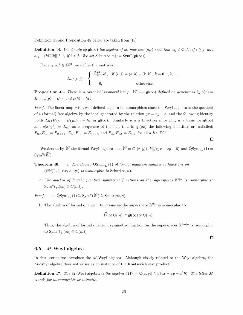
Definition 44 and Proposition 45 below are taken from [18].

Definition 44. We denote by gl(∞) the algebra of all matrices (aij) such that aij ∈ C[[~]] if i ≥ j, and

aij ∈ (~C[[~]])j−i, if i < j. We set Schur(∞, n) := Symn(gl(∞)).

For any a, b ∈ Z≥0, we define the matrices

Ea,b(i, j) =

(b+k)!k! ~b, if (i, j) = (a, b) + (k, k), k = 0, 1, 2, . . .

0, otherwise.

Proposition 45. There is a canonical isomorphism ρ : W −→ gl(∞) defined on generators by ρ(x) =

E1,0, ρ(y) = E0,1 and ρ(~) = ~I.

Proof. The linear map ρ is a well defined algebra homomorphism since the Weyl algebra is the quotient

of a (formal) free algebra by the ideal generated by the relation yx = xy + ~, and the following identity

holds E0,1E1,0 = E1,0E0,1 + ~I in gl(∞). Similarly ρ is a bijection since Ea,b is a basis for gl(∞)

and ρ(xayb) = Ea,b as consequence of the fact that in gl(∞) the following identities are satisfied:

E0,aE0,1 = E0,a+1, Ea,0E1,0 = Ea+1,0 and Ea,0E0,b = Ea,b, for all a, b ∈ Z≥0.

We denote by W the formal Weyl algebra, i.e. W = C〈〈x, y〉〉[[~]]/〈yx − xy − ~〉 and QSymAn(1) =

Symn(W ).

Theorem 46. a. The algebra QSymAn(1) of formal quantum symmetric functions on

((R2)n,∑

dxi ∧ dyi) is isomorphic to Schur(∞, n).

b. The algebra of formal quantum symmetric functions on the superspaces R2|n is isomorphic to

Symn(gl(∞) ⊗ C(m)).

Proof. a. QSymAn(1) ∼= Symn(W ) ∼= Schur(∞, n).

b. The algebra of formal quantum functions on the superspace R2|n is isomorphic to

W ⊗ C(m) ∼= gl(∞) ⊗ C(m).

Thus, the algebra of formal quantum symmetric function on the superspaces R2m|n is isomorphic

to Symn(gl(∞) ⊗ C(m)).

6.5 M-Weyl algebra

In this section we introduce the M -Weyl algebra. Although closely related to the Weyl algebra, the

M -Weyl algebra does not arises as an instance of the Kontsevich star product.

Definition 47. The M -Weyl algebra is the algebra MW = C〈x, y〉[[~]]/〈yx − xy − x2~〉. The letter M

stands for meromorphic or mimetic.

26

We have the following analogue of Proposition 29

Proposition 48. The map ρ : MW −→ End(C[x][[~]]) given by ρ(x)(f) = x−1f and ρ(y)(f) = −~∂f∂x

,

for any f ∈ C[x][[~]] defines a representation of the M -Weyl algebra.

We order the letters of the M -Weyl algebra as follows: x < y < ~. Assume we are given Ai =

(ai, bi) ∈ N2, for i ∈ [n]. Set A = (A1, . . . , An) ∈ (N2)n and XAi = xaiybi , for i ∈ [n]. Using this

notation we have

Definition 49. The normal coordinates NM (A, k) of

n∏

i=1

XAi ∈ MW are defined through the identity

n∏

i=1

XAi =

min∑

k=0

NM (A, k)x|A|+(k,−k)~

k (11)

where 0 ≤ k ≤ min = min(|a|, |b|). For k > min, we set NM (A, k) = 0.

Theorem 50. Let A, k be as in the previous definition, the following identity holds

a.

NM (A, k) =∑

p⊢k

(b

p

) n−1∏

i=1

(|a>i| + |p>i|)(pi). (12)

b. Let E1, . . . , En, F1, . . . , Fn be disjoint sets such that ♯(Fi) = ai, ♯(Ei) = bi, for i ∈ [n]. Set

E = ∪Ei, F = ∪Fi and consider the set Mk of all functions f : F −→ P (E) such that

• f(x) ∩ f(y) = ∅, for all x, y ∈ F .

• If x ∈ Fi, y ∈ Ej, and y ∈ f(x), then j < i.

•∑

a∈F

♯(f(a)) = k.

then NM (A, k) = ♯(Mk).

Proof. Using induction one show that the following identity hold in the M -Weyl algebra

ybxa =

min∑

k=0

(b

k

)a(k)xa+kyb−k

~k, (13)

where min = min(a, b) . Several application of the identity (13) imply a. Notice that for given sets E, F

such that |F | = a and |E| = b,(

bk

)a(k) is equal to ♯({f : F −→ P (E) : f(x) ∩ f(y) = ∅, for all x, y ∈

F, and∑

a∈F

♯(f(a)) = k}). This shows b, for n = 1. The general formula follows from induction.

Figure 5 illustrate the combinatorial interpretation of the normal coordinates NM (A, 6) of3∏

i=1

XAi ∈ MW , it shows an example of a function contributing to NM (A, 6).

27

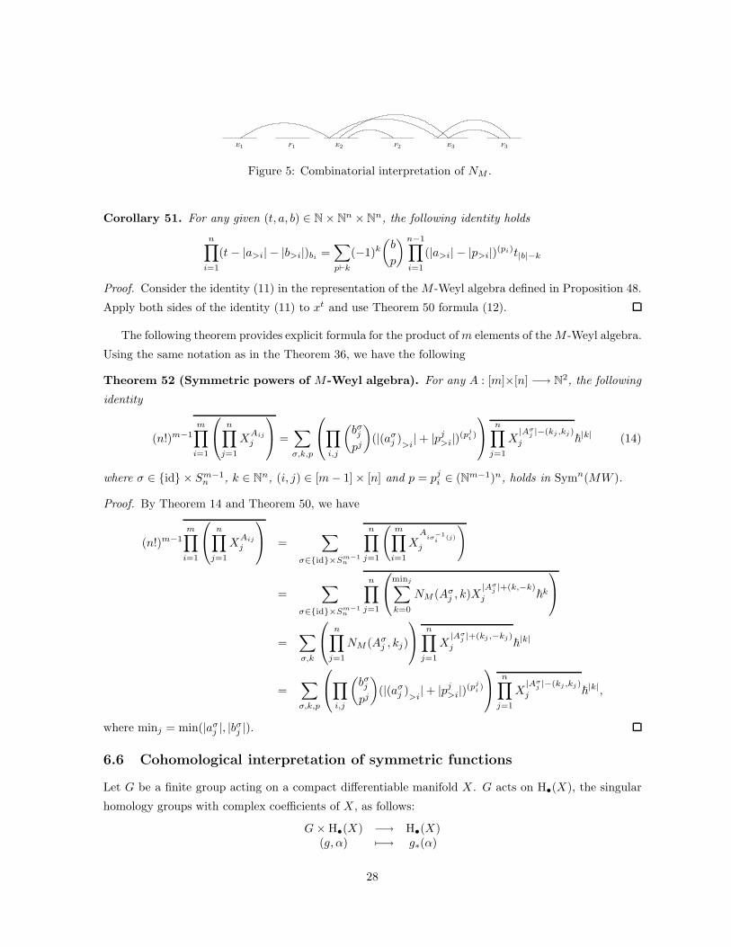
E1 F1 E2 F2 E3 F3

Figure 5: Combinatorial interpretation of NM .

Corollary 51. For any given (t, a, b) ∈ N × Nn × Nn, the following identity holds

n∏

i=1

(t − |a>i| − |b>i|)bi=∑

p⊢k

(−1)k

(b

p

) n−1∏

i=1

(|a>i| − |p>i|)(pi)t|b|−k

Proof. Consider the identity (11) in the representation of the M -Weyl algebra defined in Proposition 48.

Apply both sides of the identity (11) to xt and use Theorem 50 formula (12).

The following theorem provides explicit formula for the product of m elements of the M -Weyl algebra.

Using the same notation as in the Theorem 36, we have the following

Theorem 52 (Symmetric powers of M-Weyl algebra). For any A : [m]×[n] −→ N2, the following

identity

(n!)m−1m∏

i=1

n∏

j=1

XAij

j

=∑

σ,k,p

∏

i,j

(bσj

pj

)(|(aσ

j )>i| + |pj

>i|)(pj

i )

n∏

j=1

X|Aσ

j|−(kj ,kj)

j ~|k| (14)

where σ ∈ {id} × Sm−1n , k ∈ Nn, (i, j) ∈ [m − 1] × [n] and p = pj

i ∈ (Nm−1)n, holds in Symn(MW ).

Proof. By Theorem 14 and Theorem 50, we have

(n!)m−1m∏

i=1

n∏

j=1

XAij

j

=∑

σ∈{id}×Sm−1n

n∏

j=1

(m∏

i=1

XA

iσ−1i

(j)

j

)

=∑

σ∈{id}×Sm−1n

n∏

j=1

minj∑

k=0

NM (Aσj , k)X

|Aσj|+(k,−k)

j ~k

=∑

σ,k

n∏

j=1

NM (Aσj , kj)

n∏

j=1

X|Aσ

j|+(kj ,−kj)

j ~|k|

=∑

σ,k,p

∏

i,j

(bσj

pj

)(|(aσ

j )>i| + |pj

>i|)(pj

i)

n∏

j=1

X|Aσ

j|−(kj ,kj)

j ~|k|,

where minj = min(|aσj |, |b

σj |).

6.6 Cohomological interpretation of symmetric functions

Let G be a finite group acting on a compact differentiable manifold X . G acts on H•(X), the singular

homology groups with complex coefficients of X , as follows:

G × H•(X) −→ H•(X)(g, α) 7−→ g∗(α)

28

where g∗(α) denotes the push-forward of α by the map g. Similarly G acts on H•(X), the singular

cohomology groups with complex coefficients of X , as follows:

G × H•(X) −→ H•(X)(g, α) 7−→ g∗(α)

where g∗(α) denotes the pull-back of α by the map g. It is well-known that H•(X/G) = H•(X)G, see

[11]. Identifying H•(X)G with H•(X)G, we obtain H•(X/G) = H•(X)G. Consider Xn/Gn ⋊ K where

K ⊂ Sn and Xn = X × X × · · · × X . We have that

H•(Xn/Gn⋊ K) ∼= H•(X)⊗n/Gn

⋊ K ∼= PG,K(H•(X)).

Next theorem shows how symmetric and supersymmetric functions arise as the cohomology groups of

global orbifolds (quotient of manifolds by finite group actions). We denote by CP∞ the inductive limit

of the complex projective spaces CPn. Also, we let S1 be the unit circle in C.

Theorem 53. a. H•(((CP∞)m)n/Sn) ∼= SymAn

(m).

b. H•(((S1)m)n/Sn) ∼= Symn(∧

[θ1, . . . , θm]).

c. H•(((CP∞)m × (S1)k)n/Sn) ∼= Symn(C[x1, . . . , xn] ⊗

∧[θ1, . . . , θk]).

Proof. Recall that H•(CPn) = C[x]/(xn), see [2], which implies that H•(CP

∞) = C[x]. Thus, by the

remarks above

H•(((CP∞)m)n/Sn) ∼= ((H•(CP

∞)⊗m)⊗n)Sn∼= H•((C[x]⊗m)⊗n)Sn

∼= (C[x1, . . . , xm])⊗n/Sn∼= SymAn

(m).

Since H•(S1) ∼= C[θ]/〈θ2〉 as graded superalgebras with θ of degree 1, then

H•(((S1)m)n/Sn) ∼= ((H•(S1)⊗m)⊗n)Sn∼= (∧

[θ1, . . . , θm]⊗n)Sn∼= Symn(

∧[θ1, . . . , θm]).

Finally

H•(((CP∞)m×(S1)k)n/Sn) ∼= (H•(CP

∞)⊗m⊗H•(S1)⊗k)⊗n/Sn∼= Symn(C[x1, . . . , xm]⊗

∧[θ1, . . . , θk]).

Theorem 53 together with the quantizations of SymAn(2m) and of Symn(

∧[θ1, . . . , θm]) provided in

Sections 6.2 and 6.4 respectively, give a quantum product on the cohomology of ((CP∞)2m)n/Sn and

((S1)m)n/Sn respectively . Notice that the quantum product on H•(((CP∞)m)n/Sn) is non-commutative

and therefore is different to the quantum cohomology product defined for example in [7].

Acknowledgment

We thank Nicolas Andruskiewitsch for his advices and encouragement. We also thank Delia Flores de

Chela.

29

References

[1] J. Alev, T. J. Hodges, and J. D. Velez, Fixed rings of the Weyl algebra A1(C), Journal of algebra

130 (1990), 83–96.

[2] Raoul Bott and Loring W. Tu, Diferential forms in algebraic topology, no. 82, Springer-Velarg, New

York, 1982.

[3] P. Deligne, P. Etingof, D. Freed, L. Jeffrey, D. Kazhdan, J. Morgan, D. Morrison, and E. Witten,

Quantum fields and strings: A course for mathematicians, vol. 1, American mathematical society,

1999.

[4] Rafael Dıaz and Eddy Pariguan, Super, quantum and non-commutative species, Work in progress,

2003.

[5] , Symmetric quantum Weyl algebras, Annales Mathematiques Blaise Pascal 11 (2004), 155–

171.

[6] Vasily Dolgushev, Covariant and equivariant formality theorems, math. QA/0307212, 2003.

[7] D. Mc Duff and D. Salamon, J-holomorphic curves and quantum cohomology, vol. 6, Univesity

lecture series. AMS, Providence, Rhode Island, 1991.

[8] P. Etingof and V. Ginzburg, Symplectic reflection algebras, Calogero-Moser space, and deformed

Harish-Chandra homomorphism, Invent. Math 147 (2002), no. 2, 243–348.

[9] R. Gopakumar, S. Minwalla, and A. Strominger, Noncommutative Solitons, J. High Energy Phys.

JHEP 05-020 (2000).

[10] J. A. Green, Polynomial representations of GLn, no. 830, Lecture notes in mathematics. Springer-

Velarg, New York, 1980.

[11] F. Hirzebruch and T. Hofer, On the Euler number of an orbifold, Mathematische Annalen 286

(2002), 255–260.

[12] A. Joyal, Une theorie combinatoire des series formelles, Advances in mathematics (1981), no. 42,

1–82.

[13] , Foncteurs analytiques et especies de structures, Combinatoire enumerative. Lecture notes

in mathematics, 1234 (1986), 126–159.

[14] M. Kontsevich, Deformation Quantization of Poisson Manifolds I, math. q-alg/9709040, 1997.

[15] I. Kriz and J. P. May, Operads, algebras, modules and motives, Asterisque (1995), no. 233.

[16] I. G. Macdonald, Symmetric functions and Hall polynomials, Oxford Mathematical Monographs,

New York, 1995.

30

[17] Emil Martinec and Gregory Moore, Noncommutative Solitons on Orbifolds, hep-th/0101199, 2001.

[18] S. A. Merkulov, The Moyal product in the matrix product, math-ph/0001039, 2000.

[19] Gian-Carlo Rota, Gian-Carlo Rota on Combinatorics. Introductory papers and commentaries,

Birkhauser, Boston, 1995.

[20] R. P. Stanley, Enumerative combinatorics, vol. 2, Cambridge University Press, 1999.

[21] F. Vaccarino, The vector invariants of symmetric groups, RA/0205233, 2002.

[22] K. H. Wehrhahn, Combinatorics. An introduction, vol. 2, Carslaw Publications, Australia, 1990.

Rafael Dıaz. Instituto Venezolano de Investigaciones Cientıficas (IVIC). radiaz@ivic.ve

Eddy Pariguan. Universidad Central de Venezuela (UCV). eddyp@euler.ciens.ucv.ve

31