arX

iv:1

402.

5553

v1 [

mat

h.Q

A]

22

Feb

2014

Quantum Symmetric Functions II

Rafael Dıaz and Eddy Pariguan

February 25, 2014

Abstract

We provide an explicit description of the quantum product of multi-symmetric functionsusing the elementary multi-symmetric functions introduced by Vaccarino.

1 Introduction

Fix a characteristic zero field K. The algebro-geometric duality allow us to identify affine al-

gebraic varieties with the K-algebra of polynomial functions on it, and reciprocally, a finitely

generated algebra without nilpotent elements may be identified with its spectrum, provided

with the Zarisky topology. Affine space Kn is thus identified with the algebra of polynomials

in n-variables K[x1, ..., xn]. Consider the action of the symmetric group Sn on Kn by permu-

tation of vector entries. The quotient space Kn/Sn is the configuration space of n unlabeled

points with repetitions in K. Polynomial functions on Kn/Sn may be identified with the algebra

K[x1, ..., xn]Sn of Sn-invariant polynomials in K[x1, ..., xn]. A remarkable classical fact is that

Kn/Sn is again a n-dimensional affine space [11], indeed we have an isomorphism of algebras

K[x1, ..., xn]Sn ≃ K[e1, ..., en]

where, for α ∈ [n] = {1, ..., n}, eα is the elementary symmetric polynomial given by

eα(x1, ..., xn) =∑

|a|=α

xα =∑

a⊆[n], |a|=α

∏

j∈a

xj.

The elementary symmetric polynomials are determined by the identity

n∏

i=1

(1 + xit) =

n∑

α=0

eα(x1, ..., xn)tα.

Using characteristic functions one shows for α1, ..., αm ∈ [n] that

eα1· · · eαm =

∑

a∈Nn

c(α1, ..., αm, a)xa

1

where c(α1, ..., αm, a) is the cardinality of the subset of matrices of format n ×m with entries

in {0, 1} such that

n∑

j=1

Aij = αi for i ∈ [m],

m∑

i=1

Aij = aj for j ∈ [n].

A subtler situation arises when one considers the configuration space

(Kd)n/Sn

of n unlabeled points with repetitions in Kd, for d ≥ 2. In this case (Kd)n/Sn is not longer an

affine space, instead it is an affine algebraic variety. Polynomial functions on (Kd)n/Sn are the

so-called multi-symmetric functions, also known as vector symmetric functions or MacMahon

symmetric functions [9, 11], and coincides with the algebra of invariant polynomials

K[x11, ..., x1d, ......, xn1, ..., xnd]Sn ,

which admits a presentation of the following form

K[ eα | |α| ∈ [n] ] / In,d,

where the elementary multi-symmetric functions eα, for α = (α1, ..., αd) ∈ Nd a vector such

that |α| = α1 + ...+ αd ≤ n, are defined by the identity

n∏

i=1

(1 + xi1t1 + · · ·+ xidtd) =∑

α∈Nd, |α|≤n

eα(x11, ..., x1d, ......, xn1, ..., xnd)tα1

1 ...tαd

d .

Explicitly, the multi-symmetric function eα is given by

eα(x11, ..., x1d, ......, xn1, ..., xnd) =∑

a

xa =∑

|a|=α

∏

j∈[d]

∏

i∈aj

xij ,

where in the middle term we regard a ∈ Mn×d({0, 1}) as a matrix such that

n∑

i=1

aij = αj for j ∈ [d],

d∑

j=1

aij ≤ 1 for i ∈ [n]; and xa =

n∏

i=1

d∏

j=1

xaijij ;

and in the right hand side term we let a = (a1, ..., ad) be a d-tuple of disjoint sets aj ⊆ [n] such

that

|a| = (|a1|, ..., |ad|) = (α1, ..., αd).

It is not difficult to check that any multi-symmetric function can be written (not uniquely) as

a linear combination of products of elementary multi-symmetric functions. The non-uniqueness

is controlled by the ideal In,d. For an explicit description of In,d the reader may consult Dalbec

2

[4] and Vaccarino [12].

One checks for α1, ..., αm ∈ Nd that:

eα1· · · eαm =

∑

a∈Mn×d(N)

c(α1, ..., αm, a)xa,

where c(α1, ..., αm, a) counts the number of cubical matrices

A = (Aijl) ∈ Map([m]× [n]× [d], {0, 1})

such that

m∑

i=1

Aijl = ajl for j ∈ [n], l ∈ [d],

d∑

l=1

Aijl ≤ 1 for i ∈ [m], j ∈ [n], and

n∑

j=1

Aijl = (αi)l for i ∈ [m], l ∈ [d].

Recall that an algebra may be analyzed by describing it by generators and relations or alter-

natively, as emphasized by Rota and his collaborators, by finding a suitable basis such that the

structural coefficients are positive integers with preferably a nice combinatorial interpretation.

The second approach for the case of multi-symmetric functions was undertaken by Vaccarino

[12], and his results will be reviewed in Section 2. The main goal of this work, see Section 5,

is to generalize this combinatorial approach to multi-symmetric functions from the classical to

the quantum setting.

Quantum mechanics, the century old leading small distances physical theory, is still not

quite fully understood by mathematicians. The transition from classical to quantum mechanics

has been particularly difficult to grasp. An appealing approach to this problem is to characterize

the process of quantization as a process of deformation of a commutative Poisson algebra into

a non-commutative algebra [2]. In this approach classical phase space is replaced by quantum

phase space, where an extra dimension parametrized by a formal variable ~ is added.

The classical phase space of a Lagrangian theory is naturally endowed with a closed two-

form. In the non-degenerated case (i.e. in the symplectic case) this two-form can be inverted

given rise to a Poisson brackect on the algebra of smooth functions on phase space. In a sense,

the Poisson bracket may be regarded as a tangent vector in the space of deformations of the

algebra of functions on phase space, i.e. as an infinitesimal deformation. That this infinitesimal

deformation can be integrated into a formal deformation is a result due to Fedosov [7] for the

symplectic case, and to Kontsevich [10] for arbitrary Poisson manifolds.

3

Many Lagrangian physical theories are invariant under a continuous group of transforma-

tions; in that case the two-form on phase space is necessarily degenerated. Nevertheless, a

Lagrangian theory might be invariant under a finite group and still retain its non-degenerated

character. In the latter scenario all the relevant constructions leading to the quantum algebra

of functions on phase space are equivariant, and thus give rise to a quantum algebra of invariant

functions under the finite group. We follow this path along this work, being as explicit and

calculative as possible. Our main aim is thus to provide foundations as well as practical tools

for dealing with quantum symmetric functions.

2 Multi-Symmetric Functions

In this section we introduce Vaccarino’s multi-symmetric functions eα(p) which are defined in

analogy with the elementary multi-symmetric functions of the Introduction, a yet the definition

is general enough to account for the symmetrization of arbitrary polynomial functions [12].

Fix a, n, d ∈ N+. Let y1, ..., yd and t1, ..., ta be a pair of sets of commuting independent

variables over K. For α = (α1, ..., αa) ∈ Na we set

|α| =a∑

i=1

αi and tα =

a∏

i=1

tαi

i .

For q ∈ K[y1, ..., yd] and i ∈ [n] we let q(i) = q(xi1, ..., xid) be the polynomial obtained

by replacing each appearance of yj in q by xij , for j ∈ [d]. For example, for n = 2 and

q = y1y2y3 ∈ R[y1, y2, y3] we have that

q(1) = x11x12x13 and q(2) = x21x22x23.

Definition 1. Consider α ∈ Na such that |α| ≤ n, and p = (p1, ..., pa) ∈ K[y1, ..., yd]

a. The

multi-symmetric functions eα(p) ∈ K[(Kd)n]Sn are determined by the identity:

n∏

i=1

(1 + p1(i)t1 + · · ·+ pa(i)ta) =∑

|α|≤n

eα(p)tα.

Example 2. For n = 3 and p = (y1y2, y3y4), we have that e(1,1)(y1y2, y3y4) is equal to

x13x14x21x22 + x21x22x33x34 + x23x24x31x32+x11x12x33x34 + x13x14x31x32 + x11x12x23x24,

and e(2,1)(y1y2, y3y4) = x11x12x21x22x33x34 + x11x12x23x24x31x32 + x13x14x21x22x31x32.

Example 3. For p = (y1, ..., yd) and α ∈ Nd with |α| ∈ [n], the multi-symmetric functions

eα(y1, ..., yd) are the elementary multi-symmetric functions defined in the Introduction.

Next couple of Lemmas follow directly from Definition 1.

4

Lemma 4. Let α ∈ Na be such that |α| ≤ n, and let p = (p1, ..., pa) ∈ K[y1, ..., yd]

a. The

multi-symmetric function eα(p) is given by the combinatorial identity

eα(p) =∑

c

a∏

l=1

∏

i∈cl

pl(i),

where c = (c1, ..., ca) is a tuple of disjoint subsets of [n], with |c| = (|c1|, ..., |ca|) = α.

Recall that the symmetrization map K[(Kd)n] −→ K[(Kd)n]Sn sends f to

∑

σ∈Sn

f ◦ σ,

where we regard σ ∈ Sn as a map σ : (Kd)n −→ (Kd)n.

Lemma 5. Let α ∈ Na be such that |α| ≤ n, and p = (p1, ..., pa) ∈ K[y1, ..., yd]

a. The multi-

symmetric function eα(p) is the symmetrization of the polynomial

p1(1)...p1(α1)......pi(i−1∑

l=1

αl + 1)...pi(i∑

l=1

αl)......pa(a−1∑

l=1

αl + 1)...pa(a∑

l=1

αl).

Lemma 6. Let p = (p1, ..., pa) ∈ K[y1, ..., yd]a be expanded in monomials as

p1 =∑

j1∈[k1]

c1j1m1j1 , ........, pa =∑

ja∈[ka]

cajamaja.

Then

eα(p) =∑

β∈N|k|, r(β)=α

eβ(m)cβ ,

where m = (m11, ...,m1k1 , ......,ma1, ...,maja), c = (c11, ..., c1k1 , ......., ca1 , ..., caka), and for

β = (β11, ..., β1k1 , ......., βa1 , ..., βaka) ∈ N|k| we set

r(β) = (β11 + · · · + β1k1 , ........., βa1 + · · ·+ βaka).

Proof. Let |k| = k1 + · · ·+ ka and ct = (c11t1, ..., c1k1t1, ......., ca1t1, ..., caka ta). Then

∑

α∈Na, |α|≤n

eα(p)tα =

n∏

i=1

1 +∑

j1∈[k1]

c1j1m1j1(i)t1 + · · ·+∑

ja∈[ka]

cajamaja(i)ta

=∑

β∈N|k|, |β|≤n

eβ(m)(ct)β =∑

β∈N|k|, |β|≤n

eβ(m)cβtr(β).

Thus we get that

eα(p) =∑

β∈N|k|, r(β)=α

eβ(m)cβ .

5

The following result due to Vaccarino [12] provides an explicit formula for the product of

multi-symmetric functions. We include the proof since the same technique carries over to the

more involved quantum case.

Theorem 7. Fix a, b, n ∈ N+, p ∈ K[y1, ..., yd]

a, and q ∈ K[y1, ..., yd]b. Let α ∈ N

a and β ∈ Nb

be such that |α|, |β| ≤ n. Then we have that:

eα(p)eβ(q) =∑

γ∈L(α,β,n)

eγ(p, q, pq), where:

• (p, q, pq) = (p1, ..., pa, q1, ..., qb, p1q1, ..., p1qb, ......, paq1, ..., paqb).

• L(α, β, n) is the set of matrices γ ∈ Map([0, a] × [0, b],N) such that:

γ00 = 0, |γ| =a∑

l=0

b∑

r=0

γlr ≤ n,

b∑

r=0

γlr = αl for l ∈ [a], and

a∑

l=0

γlr = βr for r ∈ [b].

Proof. Identify the matrix γ with the vector

γ = (0, γ01, ..., γ0b, γ10, ..., γa0, γ20, ..., γ2b, ......, γa0, ..., γab).

We have that∑

|α|,|β|≤n

eα(p)eβ(q)tαsβ

is equal to

=

∑

|α|≤n

eα(p)tα

∑

|β|≤n

eβ(q)sβ

=

n∏

i=1

(

1 +

a∑

l=1

pl(i)tl

)

n∏

i=1

(

1 +

b∑

r=1

qr(i)sr

)

=

n∏

i=1

(

1 +

a∑

l=1

pl(i)tl

)(

1 +

b∑

r=1

qr(i)sr

)

=n∏

i=1

(

1 +a∑

l=1

pl(i)tl +b∑

r=1

qr(i)sr +a∑

l=1

b∑

r=1

pl(i)qr(i)tlsr

)

=

n∏

i=1

(

1 +

a∑

l=1

pl(i)wl0 +

b∑

r=1

qr(j)w0r +

a∑

l=1

b∑

r=1

pl(i)qr(i)wlr

)

=∑

γ

eγ(p, q, pq)wγ ,

where for γ ∈ L(α, β, n) we set

wγ =a∏

l=0

b∏

r=0

wγlrlr =

a∏

l=0

b∏

r=0

(tlsr)γlr =

a∏

l=0

b∏

r=0

tγlrl sγlrr ,

6

using the conventions

t0 = s0 = 1, wlr = tlsr for l, r ≥ 0.

For wγ to be equal to tαsβ we must have that

wγ =

a∏

l=0

b∏

r=0

tγlrl sγlrr =

a∏

l=1

t

b∑

r=0

γlr

l

b∏

r=1

s

a∑

l=0

γlr

r

=

(

a∏

l=1

tαl

l

)(

b∏

k=1

sβrr

)

.

Thus we conclude that

b∑

r=0

γlr = αl for l ∈ [a], anda∑

l=0

γlr = βr for r ∈ [b].

Graphically, a matrix γ ∈ L(α, β, n) is represented as

0 γ01 γ02 γ03 · · · γ0bγ10 γ11 γ12 γ13 · · · γ1b −→ α1

γ20 γ21 γ22 γ23 · · · γ2b −→ α2...

......

......

......

......

...γa0 γa1 γa2 γa3 · · · γab −→ αa

↓ ↓ ↓ ↓β1 β2 β3 · · · βb

where the horizontal and vertical arrows represent, respectively, row and column sums.

Example 8. For n = 3, p = (y1y2, y1) and q = (y1y2, y3) we have that:

e(1,1)(y1y2, y1)e(2,1)(y1y2, y3) =∑

γ

eγ(y1y2, y1, y1y2, y3, y21y

22, y1y2y3, y

21y2, y1y3),

where γ = (γ10, γ20, γ01, γ02, γ11, γ12, γ21, γ22) ∈ N8 is such that |γ| ≤ 3 and

γ10 + γ11 + γ12 = 1, γ20 + γ21 + γ22 = 1, γ01 + γ11 + γ21 = 2, γ02 + γ12 + γ22 = 1.

Looking at the solutions in N of the system of linear equations above we obtain that:

e(1,1)(y1y2, y1)e(2,1)(y1y2, y3) =

e(1,1,1)(y3, y21y

22 , y

21y2) + e(1,1,1)(y1y2, y1y2y3, y

21y2) + e(1,1,1)(y1y2, y

21y

22, y1y3).

7

Example 9. For n = 4, p = (y21y2, y32y3, y1y2y3) and q = (y31y

22y3, y

21y3, y2y3) we have that:

e(1,1,1)(y21y2, y

32y3, y1y2y3)e(1,2,1)(y

31y

22y3, y

21y3, y2y3) =

∑

γ

eγ(y21y2, y

32y3, y1y2y3, y

31y

22y3, y

21y3, y2y3, y

51y

32, y

41y2y3,

y21y22y3, y

31y

52y

23 , y

42y

23 , y1y

42y3, y

41y

32y

23 , y

31y2y

23, y

21y

22y3),

where γ = (γ10, γ20, γ30, γ01, γ02, γ03, γ11, γ12, γ13, γ21, γ22, γ23, γ31, γ32, γ33) ∈ N15 is such that

|γ| ≤ 4 and

γ10 + γ11 + γ12 + γ13 = 1, γ20 + γ21 + γ22 + γ23 = 1, γ30 + γ31 + γ32 + γ33 = 1,

γ01 + γ11 + γ21 + γ31 = 1, γ02 + γ12 + γ22 + γ32 = 2, γ03 + γ13 + γ23 + γ33 = 1.

Looking at the solutions in N of the system of linear equations above we obtain that:

e(1,1,1)(y21y2, y

32y3, y1y2y3)e(1,2,1)(y

31y

22y3, y

21y3, y2y3) =

e(1,1,1,1)(y2y3, y41y2y3, y

42y

23, y1y2y3) + e(1,1,1,1)(y2y3, y

41y2y3, y

31y

52y

23 , y

31y2y

23) +

e(1,1,1,1)(y2y3, y51y

32 , y

42y

23 , y

31y2y

23) + e(1,1,1,1)(y

21y3, y

21y

22y3, y

42y

23 , y

41y

32y

23) +

e(1,1,1,1)(y21y3, y

21y

22y3, y

31y

52y

23, y

31y2y

23) + e(1,1,1,1)(y

21y3, y

41y2y3, y1y

42y3, y

41y

32y

23) +

e(1,1,1,1)(y21y3, y

41y2y3, y

31y

52y

23, y

21y

22y3) + e(1,1,1,1)(y

21y3, y

51y

32, y1y

42y3, y

31y2y

23) +

e(1,1,1,1)(y21y3, y

51y

32, y

42y

23, y

21y

22y3) + e(1,1,1,1)(y

31y

22y3, y

21y

22y3, y

42y

23, y

31y2y

23) +

e(1,1,1,1)(y31y

22y3, y

41y2y3, y1y

32y

23, y

21y

22y3) + e(1,1,1,1)(y

31y

22y3, y

41y2y3, y

32y

23 , y

21y

22y3).

3 Review of Deformation Quantization

In this section we review a few needed notions on deformation quantization. We assume the

reader to be somewhat familiar with Kontsevich’s work [10], although that level of generality

is not necessary to understand the applications to the quantization of canonical phase space.

A Poisson bracket [6, 13] on a smooth manifold M is a R-bilinear antisymmetric map

{ , } : C∞(M)×C∞(M) −→ C∞(M),

where C∞(M) is the space of real-valued smooth functions on M , and for f, g, h ∈ C∞(M) the

following identities hold:

{f, gh} = {f, g}h + g{f, h} and {f, {g, h}} = {{f, g}, h} + {g, {f, h}}.

A manifold equipped with a Poisson bracket is called a Poisson manifold. The Poisson bracket

{ , } is determined by an antisymmetric bilinear form α on T ∗M , i.e. by the Poisson bi-vector

α ∈∧2 TM given in local coordinates (x1, x2, · · · , xd) on M by

αij = {xi, xj}.

8

The bi-vector α determines the Poisson bracket as follows

{f, g} = α(df, dg) =∑

i,j∈[d]

αij∂f

∂xi

∂g

∂xj, for f, g ∈ C∞(M).

If the Poisson bi-vector αij is non-degenerated (i.e. det(αi,j) 6= 0) the Poisson manifold M is

called symplectic.

Example 10. The space R2d is a symplectic Poisson manifold with Poisson bracket given in

the linear coordinates (x1, ..., xd, y1, ..., yd) by

{f, g} =

d∑

i=1

(

∂f

∂xi

∂g

∂yi−

∂f

∂yi

∂g

∂xi

)

, for f, g ∈ C∞(R2d).

Equivalently, the Poisson bracket { , } on C∞(R2d) is determined by the identities:

{xi, xj} = 0, {yi, yj} = 0, and {xi, yj} = δij , for i, j ∈ [d].

This example is the so-called canonical phase space with n degrees of freedom.

Example 11. Let (g, [ , ]) be a Lie algebra over R of dimension d. The dual vector space g∗

is a Poisson manifold with Poisson bracket given on f, g ∈ C∞(g∗) by

{f, g}(α) = 〈α, [dαf, dαg]〉,

where α ∈ g∗, and the differentials dαf and dαg are regarded as elements of g via the identifi-

cations T ∗αg

∗ = g∗∗ = g. Choose a linear basis e1, ..., ed for g. The structural coefficients ckij

of g are given, for i, j, k ∈ [d], by

[ei, ej ] =d∑

k=1

ckijek.

Let (x1, ..., xd) be the linear system of coordinates on g∗ relative to the basis e1, ..., ed of g. The

Poisson bracket is determined by continuity and the identities

{xi, xj} =d∑

k=1

ckijxk.

A formal deformation, or deformation quantization, of a Poisson manifold M is an associa-

tive product, called the star product,

⋆ : C∞(M)[[~]] ⊗R[[~]] C∞(M)[[~]] −→ C∞(M)[[~]]

defined on the space C∞(M)[[~]] of formal power series in ~ with coefficients in C∞(M) such

that the following conditions hold for f, g ∈ C∞(M):

9

• f ⋆ g =

∞∑

n=0

Bn(f, g)~n, where the maps

Bn( , ) : C∞(M)× C∞(M) −→ C∞(M)

are bi-differential operators.

• f ⋆ g = fg + 12{f, g}~ + O(~2), where O(~2) stand for terms of order 2 and higher in

the variable ~.

Kontsevich in [10] constructed a ⋆-product for any finite dimensional Poisson manifold. For

linear Poisson manifolds the Kontsevich ⋆-product goes as follows. Fix a Poisson manifold

(Rd, α), the Kontsevich ⋆-product is given on f, g ∈ C∞(M) by

f ⋆ g =∞∑

n=0

Bn(f, g)~n

n!=

∞∑

n=0

(

∑

Γ∈Gn

ωΓBΓ(f, g)

)

~n

n!, where:

• Gn is a collection of graphs, called admissible graphs, each with 2n edges.

• For each graph Γ ∈ Gn, the constant ωΓ ∈ R is independent of d and α, and its computed

trough an integral in an appropriated configuration space.

• BΓ( , ) : C∞(Rd)× C∞(Rd) −→ C∞(Rd) is a bi-differential operator associated to the

graph Γ ∈ Gn and the Poisson bi-vector α. The definition of the operators BΓ( , ) is

quite explicit and fairly combinatorial in nature.

Remark 12. Kontsevich himself have highlighted the fact that explicitly computing the inte-

grals defining the constants ωΓ is a daunting task currently beyond reach. One can however use

the symbols ωΓ as variables, and they will defined a deformation quantization (with an extended

ring of constants) as soon as this variables satisfy a certain system of quadratic equations [5].

We are going to use the Kontsevich ⋆-product in a slightly modified form.

Let G =∞⊔

n=0

Gn and for Γ ∈ G, set Γ = n if and only if Γ ∈ Gn.

With this notation the Kontsevich ⋆-product is given on functions f, g ∈ C∞(Rd) by

f ⋆ g =∑

Γ∈G

ωΓ

Γ!BΓ(f, g)~

Γ.

Remark 13. The Kontsevich ⋆-product is defined over R since cΓ ∈ R. If α is a regular

Poisson bi-vector, i.e. the entries αij of the Poisson bi-vector are polynomial functions, then

the ⋆-product on C∞(Rd) restricts to a well-defined ⋆-product on the space R[x1, ..., xd] of

polynomial functions on Rd. We are interested in the quantization of symmetric polynomial

functions, thus we assume that α is regular Poisson bi-vector and work with quantum algebra

(R[x1, ..., xd], ⋆).

10

4 Quantum Symmetric Functions

Let Sn be the symmetric group on n letters. For each subgroup K ⊆ Sn, consider the Polya

functor PK : R-alg −→ R-alg from the category of associative R-algebras to itself, defined on

objects as follows [5]. Let A be a R-algebra, the underlying vector space of PKA is given by

PKA = (A⊗n)K = A⊗n / 〈 a1 ⊗ · · · ⊗ an − aσ1 ⊗ · · · ⊗ aσn | ai ∈ A, σ ∈ K 〉.

Elements of PKA are written as a1 ⊗ · · · ⊗ an. For aij ∈ A, the following identity determines

the product on PKA:

|K|m−1m∏

i=1

n⊗

j=1

aij

=∑

σ∈{1}×Km−1

n⊗

j=1

(

m∏

i=1

aiσ−1

i(j)

)

.

The Polya functor PK is also known as the co-invariants functor. The invariants functor

IK : R-alg −→ R-algA −→ (A⊗n)K

is given on objects by

(A⊗n)K = { a ∈ A⊗n | ga = a for g ∈ K }.

The product on (A⊗n)K comes from the inclusion (A⊗n)K ⊂ A⊗n.

The functors IK and PK are naturally isomorphic to each other [5].

Suppose a finite group K acts on a Poisson manifold M , and that the induced action of

K on (C∞(M)[[~]], ⋆) is by algebra automorphisms, then we define the algebra of quantum

K-symmetric functions on M as

(C∞(M)[[~]], ⋆)K ≃ (C∞(M)[[~]], ⋆)K .

Let (Rd, α) be a regular Poisson manifold. The Cartesian product of Poisson manifolds

is naturally endowed with the structure of a Poisson manifold, thus we get a regular Poisson

manifold structure on (Rd)n. We use the following coordinates on the n-fold Cartesian product

of Rd with itself:

(Rd)n = { (x1, ..., xn) | xi = (xi1, ..., xid) ∈ Rd, xij ∈ R, (i, j) ∈ [n]× [d] }.

The ring of regular functions on (Rd)n is the ring of polynomials on dn commutative variables:

R[(Rd)n] = R[x11, ..., x1d, ......, xn1, ..., xnd].

11

Consider another set of commutative variables y1, ..., yd. Recall from Section 2 that for f ∈

R[y1, ..., yd] and i ∈ [n] we set f(i) = f(xi1, ..., xid) ∈ R[xi1, ..., xid] ⊆ R[(Rd)n].

The Poisson bracket on (Rd)n is determined by the following identities

{xki, xlj} = δklαij(k), for i, j ∈ [d] and k, l ∈ [n]

where the coordinates αij of the Poisson bivector α =∑

αij∂i∧∂j are regarded as polynomials

in R[y1, ..., yn]. The Poisson bracket on (Rd)n is Sn-invariant, indeed for σ ∈ Sn we have that:

{xσki, xσlj} = δσk,σlαij(σk) = σ(δklαij(k)).

Next results [5] provide a natural construction of groups acting as algebra automorphisms

on the algebras (R[Rd][[~]], ⋆).

Theorem 14. Let (Rd, { , }) be a regular Poisson manifold, and K be a subgroup of Sd such

that the Poisson bracket { , } is K-equivariant. Then the action of K on (R[Rd][[~]], ⋆) is by

algebra automorphisms.

Corollary 15. Let (Rd, { , }) be a regular Poisson manifold and consider a subgroup K ⊆ Sn.

Then K acts by algebra automorphisms on (R[(Rd)n][[~]], ⋆).

Definition 16. Let (Rd, { , }) be a regular Poisson manifold. The algebra of quantum sym-

metric functions on (Rd)n is given by

(R[(Rd)n][[~]], ⋆)Sn ≃ (R[(Rd)n][[~]], ⋆)Sn .

Example 17. Consider R2d with its canonical symplectic Poisson structure, then (R2d)n is also

a symplectic Poisson manifold. Choose coordinates on (R2d)n as follows:

(R2d)n = { (x1, y1, ..., xn, yn) | xi = (xi1, ..., xid), yi = (yi1, ..., yid), xij , yij ∈ R } .

The Sn-invariant Poisson bracket on (R2d)n is given for i, j ∈ [d] and k, l ∈ [n] by

{xki, xlj} = 0, {yki, ylj} = 0 and {xki, ylj} = δklδij .

Example 18. Let g be a d-dimensional Lie algebra over R and g∗ its dual vector space. Then g

∗

is a Poisson manifold, and therefore (g∗)n is also a Poisson manifold. The Sn-invariant Poisson

bracket on (g∗)n is given, for i, j ∈ [d] and k, l ∈ [n], by

{xki, xlj} = δkl

d∑

m=0

cmijxkm

where cmij are the structural coefficients of g.

12

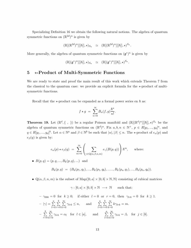
Specializing Definition 16 we obtain the following natural notions. The algebra of quantum

symmetric functions on (R2d)n is given by

(R[(R2d)n][[~]], ⋆)Sn ≃ (R[(R2d)n][[~]], ⋆)Sn .

More generally, the algebra of quantum symmetric functions on (g∗)n is given by

(R[(g∗)n][[~]], ⋆)Sn ≃ (R[(g∗)n][[~]], ⋆)Sn .

5 ⋆-Product of Multi-Symmetric Functions

We are ready to state and proof the main result of this work which extends Theorem 7 from

the classical to the quantum case: we provide an explicit formula for the ⋆-product of multi-

symmetric functions.

Recall that the ⋆-product can be expanded as a formal power series en ~ as:

f ⋆ g =

∞∑

n=0

Bn(f, g)~n

n!.

Theorem 19. Let (Rd, { , }) be a regular Poisson manifold and (R[(Rd)n][[~]], ⋆)Sn be the

algebra of quantum symmetric functions on (Rd)n. Fix a, b, n ∈ N+, p ∈ R[y1, ..., yd]

a, and

q ∈ R[y1, ..., yd]b. Let α ∈ N

a and β ∈ Nb be such that |α|, |β| ≤ n. The ⋆-product of eα(p) and

eβ(q) is given by:

eα(p) ⋆ eβ(q) =

∞∑

m=0

∑

γ∈Q(α,β,n,m)

eγ(B(p, q))

~m, where:

• B(p, q) = (p, q, ..., Bk(p, q), ...) and

Bk(p, q) = (Bk(p1, q1), ..., Bk(p1, qb), ......, Bk(pa, q1), ..., Bk(pa, qb)).

• Q(α, β, n,m) is the subset of Map([0, a] × [0, b]× N,N) consisting of cubical matrices

γ : [0, a]× [0, b] × N −→ N such that:

– γ00k = 0 for k ≥ 0; if either l = 0 or r = 0, then γlrk = 0 for k ≥ 1.

– |γ| =a∑

l=0

b∑

r=0

∞∑

k=0

γlrk ≤ n, anda∑

l=0

b∑

r=0

∞∑

k=0

kγlrk = m.

–b∑

r=0

∞∑

k=0

γlrk = αl for l ∈ [a], anda∑

l=0

∞∑

k=0

γlrk = βr for j ∈ [b].

13

Proof. We have that

∑

|α|,|β|≤n

∞∑

m=0

Bm(eα(p), eβ(q))tαsβ~m =

∑

|α|,|β|≤n

(eα(p) ⋆ eβ(q)) tαsβ =

∑

|α|≤n

eα(p)tα

⋆

∑

|β|≤n

eβ(q)sβ

=

n∏

i=1

(

1 +

a∑

l=1

pl(i)tl

)

⋆

n∏

i=1

(

1 +

b∑

r=1

qr(i)sr

)

=

n∏

i=1

(

1 +

a∑

l=1

pl(i)tl

)

⋆

(

1 +

b∑

r=1

qr(i)sr

)

=

n∏

i=1

(

1 +

a∑

l=1

pl(i)tl +

b∑

r=1

qr(i)sr +

a∑

l=1

b∑

r=1

pl(i) ⋆ qr(i)tlsr

)

=

n∏

i=1

(

1 +a∑

l=1

pl(i)tl +b∑

r=1

qr(i)sr +a∑

l=1

b∑

r=1

∞∑

k=0

Bk(pl(i), qr(i))tlsr~k

)

=

n∏

i=1

(

1 +

a∑

l=1

pl(i)wl00 +

b∑

r=1

qr(i)w0r0 +

a∑

l=1

b∑

r=1

∞∑

k=0

Bk(pl(i), qr(i))wlrk

)

=

∑

γ∈Q(α,β,n,m)

eγ(B(p, q))wγ , where:

wγ =

a∏

l=0

b∏

r=0

∞∏

k=0

wγlrklrk =

a∏

l=0

b∏

r=0

∞∏

k=0

(tlsr~k)γlrk =

a∏

l=0

b∏

r=0

∞∏

k=0

tγlrkl sγlrkr ~kγlrk ,

and we are using the conventions

t0 = s0 = 1, wruk = trsu~k for r, u,m ≥ 0.

For wγ to be equal to tαsβ~m we must have

(

a∏

l=0

tαl

l

)(

b∏

r=0

sβrr

)

~m =

a∏

l=0

b∏

r=0

∞∏

k=0

tγlrkl sγlrkr ~kγlrk =

(

a∏

l=0

b∏

r=0

∞∏

k=0

tγlrkl

)(

a∏

l=0

b∏

r=0

∞∏

k=0

sγlrkr

)(

a∏

l=0

b∏

r=0

∞∏

k=0

~kγlrk

)

=

a∏

l=1

t

b∑

r=0

∞∑

k=0

γlrk

l

b∏

r=1

s

a∑

l=0

∞∑

k=0

γlrk

r

~

a∑

l=0

b∑

r=0

∞∑

k=0

kγlrk.

and thus we conclude that

b∑

r=0

∞∑

k=0

γlrk = αl for l ∈ [a],a∑

l=0

∞∑

k=0

γlrk = βr for j ∈ [b],a∑

l=0

b∑

r=0

∞∑

k=0

kγlrk = m.

14

Corollary 20. With the assumptions of Theorem 19, the Poisson bracket of the multi-symmetric

functions eα(p) and eβ(q) is given by

{eα(p), eβ(q)} = 2∑

γ∈Q(α,β,n,1)

eγ(B(p, q)).

Proof. Follows from Theorem 19 and the identity

{eα(p), eβ(q)} = 2∂

∂~(eα(p) ⋆ eα(q)) |~=0 .

For our next result we regard (R[(Rd)n][[~]], ⋆)Sn as a topological algebra with topology

induced by the inclusion

(R[(Rd)n][[~]], ⋆)Sn ⊆ (R[(Rd)n][[~]], ⋆),

where a fundamental system of neighborhoods of 0 ∈ R[(Rd)n][[~]] is given by the decreasing

family of sub-algebras

R[(Rd)n][[~]] ⊇ ~R[(Rd)n][[~]] ⊇ ......... ⊇ ~nR[(Rd)n][[~]] ⊇ ..........

Recall from the introduction that the elementary multi-symmetric functions ek, for k ∈ Nd

with |k| ≤ n, are defined by the identity

n∏

i=1

(1 + xi1t1 + · · ·+ xidtd) =∑

k∈Nd, |k|≤n

ektk.

Similarly, the homogeneous multi-symmetric functions hk, for k = (k1, ..., kd) ∈ Nd, are

defined by the identityn∏

i=1

1

1− xi1t1 − · · · − xidtd=

∑

k∈Nd

hktk.

Let Md be the set of (non-trivial) monomials in the variables y1, ..., yd. The power sum

symmetric function e1(m) is given, for m ∈ Md, by

e1(m) = m(1) + · · · + m(d).

Theorem 21. The elementary multi-symmetric functions ek for |k| ≤ n, the homogeneous

multi-symmetric functions hk for |k| ≤ n, and the power sum multi-symmetric functions e1(m)

with m ∈ Md a monomial of degree less than or equal to n, together with ~ generate, respec-

tively, the topological algebra (R[(Rd)n][[~]], ⋆)Sn .

15

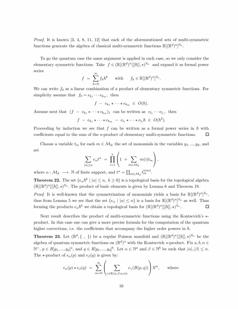
Proof. It is known [3, 4, 8, 11, 12] that each of the aforementioned sets of multi-symmetric

functions generate the algebra of classical multi-symmetric functions R[(Rd)n]Sn .

To go the quantum case the same argument is applied in each case, so we only consider the

elementary symmetric functions. Take f ∈ (R[(Rd)n][[~]], ⋆)Sn and expand it as formal power

series

f =∞∑

k=0

fk~k with fk ∈ R[(Rd)n]Sn .

We can write f0 as a linear combination of a product of elementary symmetric functions. For

simplicity assume that f0 = ek1 · · · ekm , then

f − ek1 ⋆ · · · ⋆ ekm ∈ O(~).

Assume next that (f − ek1 ⋆ · · · ⋆ ekm)1 can be written as el1 · · · elr , then

f − ek1 ⋆ · · · ⋆ ekm − el1 ⋆ · · · ⋆ elr~ ∈ O(~2).

Proceeding by induction we see that f can be written as a formal power series in ~ with

coefficients equal to the sum of the ⋆-product of elementary multi-symmetric functions.

Choose a variable tm for each m ∈ Md, the set of monomials in the variables y1, ..., yd, and

set∑

|α|≤n

eαtα =

n∏

i=1

1 +∑

m∈Md

m(i)tm

,

where α : Md −→ N of finite support, and tα =∏

m∈Mdtα(m)m .

Theorem 22. The set {eα~k | |α| ≤ n, k ≥ 0} is a topological basis for the topological algebra

(R[(Rd)n][[~]], ⋆)Sn . The product of basic elements is given by Lemma 6 and Theorem 19.

Proof. It is well-known that the symmetrization of monomials yields a basis for R[(Rd)n]Sn ,

thus from Lemma 5 we see that the set {eα | |α| ≤ n} is a basis for R[(Rd)n]Sn as well. Thus

forming the products eα~k we obtain a topological basis for (R[(Rd)n][[~]], ⋆)Sn .

Next result describes the product of multi-symmetric functions using the Kontsevich’s ⋆-

product. In this case one can give a more precise formula for the computation of the quantum

higher corrections, i.e. the coefficients that accompany the higher order powers in ~.

Theorem 23. Let (Rd, { , }) be a regular Poisson manifold and (R[(Rd)n][[~]], ⋆)Sn be the

algebra of quantum symmetric functions on (Rd)n with the Kontsevich ⋆-product. Fix a, b, n ∈

N+, p ∈ R[y1, ..., yd]

a, and q ∈ R[y1, ..., yd]b. Let α ∈ N

a and β ∈ Nb be such that |α|, |β| ≤ n.

The ⋆-product of eα(p) and eβ(q) is given by:

eα(p) ⋆ eβ(q) =∞∑

m=0

∑

γ∈K(α,β,n,m)

eγ(B(p, q))

~m, where:

16

• B(p, q) = (p, q, ......, ωΓ

Γ!BΓ(p, q), ......) and

BΓ(p, q) = (BΓ(p1, q1), ..., BΓ(p1, qb), ..., BΓ(pa, q1), ..., BΓ(pa, qb)) .

The polynomial BΓ(pi, qj) results of applying Kontsevich’s bi-differential operator BΓ to

the pair (pi, qj).

• K(α, β, n,m) is the subset of Map([0, a] × [0, b]×G,N) consisting of maps

γ : [0, a] × [0, b]×G −→ N such that:

– γ00Γ = 0; if either l = 0 or r = 0, then γlrΓ = 0 for Γ ≥ 1.

– |γ| =a∑

l=0

b∑

r=0

∑

Γ∈GγlrΓ ≤ n, and

a∑

l=0

b∑

r=0

∑

Γ∈GΓγlrΓ = m.

–b∑

r=0

∑

Γ∈GγlrΓ = αl for l ∈ [a], and

a∑

l=0

∑

Γ∈GγlrΓ = βr for j ∈ [b].

Proof. We have that

∑

|α|,|β|≤n

∞∑

m=0

Bm(eα(p), eβ(q))tαsβ~m =

∑

|α|,|β|≤n

(eα(p) ⋆ eβ(q)) tαsβ =

∑

|α|≤n

eα(p)tα

⋆

∑

|β|≤n

eβ(q)sβ

=n∏

i=1

(

1 +a∑

l=1

pl(i)tl

)

⋆

(

1 +b∑

r=1

qr(i)sr

)

=

n∏

i=1

(

1 +

a∑

l=1

pl(i)tl +

b∑

r=1

qr(i)sr +

a∑

l=1

b∑

r=1

pl(i) ⋆ qr(i)tlsr

)

=

n∏

i=1

(

1 +

a∑

l=1

pl(i)tl +

b∑

r=1

qr(i)sr +

a∑

l=1

b∑

r=1

∑

Γ∈G

ωΓ

Γ!BΓ(pl(i), qr(i))tlsr~

Γ

)

=

n∏

i=1

(

1 +a∑

l=1

pl(i)wl0∅ +b∑

r=1

qr(i)w0r∅ +a∑

l=1

b∑

r=1

∑

Γ∈G

ωΓ

Γ!BΓ(pl(i), qr(i))wrkΓ

)

=

∑

γ∈K(α,β,n,m)

eγ(B(p, q))wγ , where:

wγ =a∏

l=0

b∏

r=0

∏

Γ∈G

wγlrΓlrΓ =

a∏

l=0

b∏

r=0

∞∏

Γ∈G

tγlrkl sγlrkr ~ΓγlrΓ ,

by convention ∅ stands for the unique graph in G with no edges (representing the classical

product), and

t0 = s0 = 1, wruΓ = trsu~Γ for r, u ≥ 0, Γ ∈ G.

17

For tαsβ~m = wγ we must have

(

a∏

l=0

tαl

l

)(

b∏

r=0

sβrr

)

~m =

a∏

l=0

b∏

r=0

∏

Γ∈G

tγlrkl sγlrkr ~ΓγlrΓ =

a∏

l=1

t

b∑

r=0

∑

Γ∈G

γlrΓ

l

b∏

r=1

s

a∑

l=0

∑

Γ∈G

γlrΓ

r

~

a∑

l=0

b∑

r=0

∑

Γ∈G

ΓγlrΓ.

Thus we conclude that:

b∑

r=0

∑

Γ∈G

γlrΓ = αl for l ∈ [a],

a∑

l=0

∑

Γ∈G

γlrΓ = βr for j ∈ [b],

a∑

l=0

b∑

r=0

∑

Γ∈G

ΓγlrΓ = m.

6 Symmetric Powers of the Weyl Algebras

In this section we study the case of two dimensional canonical phase space, i.e. the symplectic

manifold R2 with the canonical Poisson bracket given by

{f, g} =∂f

∂x

∂g

∂y−

∂f

∂y

∂g

∂x.

Definition 24. The Weyl algebra is given by generators and relations by

W = R〈x, y〉[[~]]/〈yx − xy − ~〉.

The deformation quantization of (R2, { , }) is well-known to be given by the Moyal product

[1]. Moreover, one has the following result.

Theorem 25. The Weyl algebra is isomorphic to the deformation quantization of polynomial

functions on R2 with the canonical Poisson structure.

Our goal in this section is to study the deformation quantization of (R2)n/Sn, which can be

identified the algebra of quantum symmetric functions

(R[x1, ..., xn, y1, ..., yn][[~]], ⋆)Sn ,

or equivalently, with the symmetric powers of the Weyl algebra

(W⊗n)/Sn.

One shows by induction [5] that the following identity holds in the Weyl algebra:

(xcyd) ⋆ (xfyg) =

min∑

k=0

Bk(xcyd, xfyg)~k =

min∑

k=0

(

d

k

)

(f)kxc+f−kyd+g−k

~k,

where min = min(d, f) and (f)k = f(f − 1)(f − 2)(f − k + 1).

18

Theorem 26. Consider R2 with its canonical Poisson structure. Fix a, b ∈ N+, and let

(xc1yd1 , ..., xcayda) ∈ R[x, y]a and (xf1yg1 , ..., xfbygb) ∈ R[x, y]b.

For α ∈ Na and β ∈ N

b we have that:

eα(xc1yd1 , ..., xcayda) ⋆ eβ(x

f1yg1 , ..., xfbygb) =

∞∑

m=0

∑

γ∈Q(α,β,n,m)

eγ(B(xc1yd1 , ..., xcayda , xf1yg1 , ..., xfbygb))

~m,

where:

B(xc1yd1 , ..., xca , yda , xf1yg1 , ..., xfbygb) =

(xc1yd1 , ..., xca , yda , xf1yg1 , ..., xfbygb , .....,

(

drk

)

(fr)kxcl+fr−kydl+gr−k, .....).

Proof. We have that:

∑

|α|,|β|≤n

∞∑

m=0

Bm(eα(xc1yd1 , ..., xcayda), eβ(x

f1yg1 , ..., xfbygb))tαsβ~m =

∑

|α|,|β|≤n

(

eα(xc1yd1 , ..., xcayda) ⋆ eβ(x

f1yg1 , ..., xfbygb))

tαsβ =

∑

|α|≤n

eα(xc1yd1 , ..., xcayda)tα

⋆

∑

|β|≤n

eβ(xf1yg1 , ..., xfbygb)sβ

=

n∏

i=1

(

1 +

a∑

l=1

xcli ydli tl

)

⋆

(

1 +

b∑

r=1

xfri ygri sr

)

=

n∏

i=1

(

1 +

a∑

l=1

xcli ydli tl +

b∑

r=1

xfri ygri sr +

a∑

l=1

b∑

r=1

xcli ydli ⋆ xfri ygri tlsr

)

=

n∏

i=1

(

1 +a∑

l=1

xcli ydli tl +

b∑

r=1

xfri ygri sr +a∑

l=1

b∑

r=1

min∑

k=0

(

drk

)

(fr)kxcl+fr−ki ydl+gr−k

i tlsr~k

)

=

n∏

i=1

(

1 +

a∑

l=1

xcli ydli wl00 +

b∑

r=1

xfri ygri w0r0 +

a∑

l=1

b∑

r=1

min∑

k=0

(

drk

)

(fr)kxcl+fr−ki ydl+gr−k

i wlrk

)

=

∑

γ∈Q(α,β,n,m)

eγ(B(xc1yd1 , ..., xca , yda , xf1yg1 , ..., xfbygb))wγ ,

where min = min{dl, fr} and wlrk = tlsr~k.

19

Corollary 27. With the assumptions of Theorem 26, the Poisson bracket of the multi-symmetric

functions eα(p) and eβ(q) is given by

{eα(p), eβ(q)} = 2∑

γ∈Q(α,β,n,1)

eγ(B(xc1yd1 , ..., xca , yda , xf1yg1 , ..., xfbygb)).

Example 28. Let p = y, q = x ∈ R[x, y]. We have that:

eα(y) ⋆ eβ(x) =∑

m≥0

∑

γ∈Q(α,β,n,m)

eγ(y, x, xy, 1)~m,

where the vectors γ = (γ100, γ010, γ110, γ111) ∈ N4 are such that |γ| ≤ n and

γ100 + γ110 + γ111 = α, γ010 + γ110 + γ111 = β, and γ111 = m.

For example, for n = 3, α = 2, β = 3, we have

e2(y) ⋆ e3(x) = e(1,2)(x, xy) + e(1,1,1)(x, xy, 1)~ + e(1,2)(x, 1)~2

since in this case γ = (γ100, γ010, γ110, γ111) ∈ N4 is such that

γ100 + γ010 + γ110 + γ111 ≤ 3, γ100 + γ110 + γ111 = 2, γ010 + γ110 + γ111 = 3, γ111 = m.

Solving this equation for m = 0, 1, 2 we, respectively, obtain

γ = (0, 1, 2, 0), γ = (0, 1, 1, 1), and γ = (0, 1, 0, 2),

yielding the desired result.

On the other hand, from Definition 1 we get that

e2(y) = y1y2 + y1y3 + y2y3, e3(x) = x1x2x3, and thus

e2(y) ⋆ e3(x) = (y1y2 + y1y3 + y2y3) ⋆ (x1x2x3) =

(x1x2x3y1y2 + x1x2x3y1y3 + x1x2x3y2y3) +

(x1x3y1 + x1x2y1 + x2x3y2 + x1x2y2 + x2x3y3 + x1x3y3)~ + (x1 + x2 + x3)~2,

which indeed is equal to

e(1,2)(x, xy) + e(1,1,1)(x, xy, 1)~ + e(1,2)(x, 1)~2.

Note that {e2(y), e3(x)} = 2e(1,1,1)(x, xy, 1).

20

Example 29. Let p = q = xy ∈ R[x, y], then we have that

eα(xy) ⋆ eβ(xy) =∑

m≥0

∑

γ∈QL(α,β,n,m)

eγ(xy, xy, x2y2, xy)~m,

where the vector γ = (γ100, γ010, γ110, γ111) ∈ N4 is such that |γ| ≤ n and

γ100 + γ110 + γ111 = α, γ010 + γ110 + γ111 = β and γ111 = m.

Thus for n = 2, α = 2, β = 1, we get

e2(xy) ⋆ e1(xy) = e(1,1)(xy, x2y2) + e(1,1)(xy, xy)~

since in this case γ = (γ100, γ010, γ110, γ111) ∈ N4 is such that

γ100 + γ010 + γ110 + γ111 ≤ 2, γ100 + γ110 + γ111 = 2, γ010 + γ110 + γ111 = 1, γ111 = m.

Solving this equation for m = 0, 1 we, respectively, obtain

γ = (1, 0, 1, 0) and γ = (1, 0, 0, 1), yielding the desired result.

From Definition 1 we have e2(xy) = x1y1x2y2, e1(xy) = x1y1 + x2y2, and thus

e2(xy) ⋆ e1(xy) = (x1y1x2y2) ⋆ (x1y1 + x2y2) = (x21y21x2y2 + x1y1x

22y

22) + 2(x1y1x2y2)~,

which indeed is equal to e(1,1)(xy, x2y2) + e(1,1)(xy, xy)~.

Note that {e2(xy), e1(xy)} = 2e(1,1)(xy, xy).

Example 30. Let n = 2, α = β = 2, then

e2(xay) ⋆ e2(xy

b) = e2(xa+1yb+1) + e(1,1)(x

a+1yb+1, xayb)~ + e2(xayb)~2.

Using Theorem 19 we have that

e2(xay) ⋆ e2(xy

b) =∑

γ∈QL(2,2,2,m)

eγ(xay, xyb, xa+1yb+1, xayb)~m,

where γ = (γ100, γ010, γ110, γ111) ∈ N4 is such that

γ100 + γ010 + γ110 + γ111 ≤ 2, γ100 + γ110 + γ111 = 2, γ010 + γ110 + γ111 = 2, γ111 = m.

Solving this equation for m = 0, 1, 2 we, respectively, obtain

γ = (0, 0, 2, 0), γ = (0, 0, 1, 1) and γ = (0, 0, 0, 2).

21

Thus we get that

e2(xay) ⋆ e2(xy

b) = e2(xa+1yb+1) + e(1,1)(x

a+1yb+1, xayb)~ + e2(xayb)~2.

On the other hand from Definition 1 we have that

e2(xay) = xa1y1x

a2y2 and e2(xy

b) = x1yb1x2y

b2.

Computing directly the ⋆-product we obtain

e2(xay) ⋆ e2(xy

b) = (xa1y1xa2y2) ⋆ (x1y

b1x2y

b2) =

xa+11 yb+1

1 xa+12 yb+1

2 + (xa1yb1x

a+12 yb+1

2 + xa+11 yb+1

1 xa2yb2)~ + xa1y

b1x

a2y

b2~

2 =

e2(xa+1yb+1) + e(1,1)(x

a+1yb+1, xayb)~ + e2(xayb)~2.

Note that {e2(xay), e2(xy

b)} = 2e(1,1)(xa+1yb+1, xayb).

We close this work stating the main problem that our research opens.

Problem 31. Describe the relations in the algebra of quantum symmetric functions.

Acknowledgment

We thank Camilo Ortiz and Fernando Novoa for helping us to develop the software used in the

examples.

References

[1] M. Bartlett, J. Moyal, The Exact Transition Probabilities of Quantum-Mechanical Oscil-

lators Calculated by the Phase-Space Method, Proc. Camb. Phil. Soc. 45 (1949) 545-553.

[2] F. Bayen, M. Flato, C. Frønsdal, A. Lichnerowicz, D. Sternheimer, Deformation theory

and quantization. I. Deformation of symplectic structures, Ann. Physics 111 (1978) 61-110.

[3] E. Briand, When is the algebra of Multisymmetric Polynomials generated by the Elemen-

tary Multisymmetric polynomials?, Beitr. Algebra Geom. 45 (2004) 353-368.

[4] J. Dalbec, Multisymmetric functions, Beitrage Algebra Geom. 40 (1999) 27-51.

[5] R. Dıaz, E. Pariguan, Quantum symmetric functions, Comm. Alg. 33 (2005) 1947-1978.

[6] J.-P. Dufour, N. Zung, Poisson Structures and Their Normal Forms, Progress in Mathe-

matics, Birkhauser, Boston 2005.

22

[7] B. Fedosov, A simple geometrical construction of deformation quantization, J. Diff. Geom.

40 (1994) 213-238.

[8] P. Fleischmann, A new degree bound for vector invariants of symmetric groups, Trans.

Amer. Math. Soc. 350 (1998) 1703-1712.

[9] I. Gelfand, M. Kapranov, A. Zelevinsky, Discriminants, Resultants, and Multidimensional

Determinants, Birkhauser, Boston 1994.

[10] M. Kontsevich, Deformation Quantization of Poisson Manifolds I, Lett. Math. Phys. 66

(2003) 157-216.

[11] I. Macdonald, Symmetric Functions and Hall Polynomials, Oxford Math. Monograph, Ox-

ford Univ. Press, Oxford 1995.

[12] F. Vaccarino, The ring of multisymmetric functions, Ann. Inst. Fourier 55 (2005) 717-731.

[13] I. Vaisman, Lectures on Geometry of Poisson Manifolds, Progress in Mathematics,

Birkhauser, Boston 1994.

ragadiaz@gmail.com

Instituto de Matematicas y sus Aplicaciones, Universidad Sergio Arboleda, Bogota, Colombia

epariguan@javeriana.edu.co

Departamento de Matematicas, Pontificia Universidad Javeriana, Bogota, Colombia

23