arX

iv:g

r-qc

/001

1111

v2 1

3 Fe

b 20

01

Quantum correlation functions and the classical

limit

Charis Anastopoulos ∗

Department of Physics, University of Maryland, College Park, MD20742, USA

February 7, 2008

Abstract

We study the transition from the full quantum mechanical descriptionof physical systems to an approximate classical stochastic one. Our maintool is the identification of the closed-time-path (CTP) generating func-tional of Schwinger and Keldysh with the decoherence functional of theconsistent histories approach. Given a degree of coarse-graining in whichinterferences are negligible, we can explicitly write a generating functionalfor the effective stochastic process in terms of the CTP generating func-tional. This construction gives particularly simple results for Gaussianprocesses. The formalism is applied to simple quantum systems, quan-tum Brownian motion, quantum fields in curved spacetime. Perturbationtheory is also explained. We conclude with a discussion on the problemof backreaction of quantum fields in spacetime geometry.

1 Classical vs. quantum probability

1.1 Introduction

The emergence of classical behaviour in quantum systems is a very importantquestion on the foundations of quantum theory. An explanation of how theclassical world emerges is absolutely essential for any scheme that has ambitionsto go beyond the operational description of the Kopenhagen interpretation. Inrecent years the programme of decoherence has provided some insight on howthis transition is effected and suggested branches of physics, where relevantphenomena are important, like quantum optics and mesoscopic physics.

From another perspective, the issue of classicalisation is of significance incosmology. We want to know how the perceived classical world is obtained froman underlying description, that is of a (presumably) quantum nature: in the

∗charis@physics.umd.edu

1

early universe, processes are assumed to be governed by quantum field theory,but later a classical hydrodynamics description suffices to capture all relevantphysics. The same question is asked for quantum gravity: only now the focusis on the emergence of classical spacetime rather than of the matter fields. Ata more technical level one is interested to know, when the semiclassical gravityapproximation (coupling classical metric variables to quantum fields) is valid.

In all such discussions, the first step is to establish what is meant by classicalbehaviour. The notion of classicality can be defined in different ways, accordingto the context. For instance:

- the absence of interferences in a given basis: in other words an approximatediagonalisation of the density matrix [1, 2, 3].- determinism or approximate determinism or some form of predictability [4, 5,6].- the validity of a hydrodynamic or thermodynamic description for a many-bodysystem [5, 7, 8].- the existence of exact or approximate superselection rules [9].

Whatever the definition of classicality might be, there is a consensus abouthow it appears. Coarse-graining is necessary. Since the underlying theory is as-sumed to be quantum theory (which is by definition non-classical), one can geta different behaviour only by examining a truncated version of the theory. Theintuitive picture for emergent classicality is that of a random phase approxima-tion: the coarser the description of the system, the more the interference phasecancel out when averaged within the coarse-grained observable. The generalquestion is then, which types of coarse-graining can regularly lead to classicalbehaviour.

In this paper, we take the attitude that a system exhibits classical behaviour,if it admits an approximate description in terms of classical probability theory.Since we are interested in systems changing in time, we ask that the evolutionof coarse-grained observables is described by probability theory: in other wordsthat it should be modeled by a stochastic process.

Quantum processes have an important difference from stochastic processes:their correlation functions are complex-valued rather than real-valued. This isequivalent to the fact that quantum mechanical evolution cannot be describedby a probability measure. In this paper, we focus on how classical correla-tion functions can be constructed from the quantum mechanical ones throughcoarse-graining, thus providing an effective stochastic description for a quan-tum system. A part of the relevant material has appeared previously in [10].This presentation is simultaneously an elaboration and a simplification of themathematical constructions performed in this reference, with an eye to possibleapplications.

2

We shall then apply this formalism in various cases. We will show that inGaussian systems, the classical limit is mostly determined by the real part ofthe quantum two-point function. We shall verify this in a number of examples:simple harmonic oscillators, the Caldeira-Leggett model of quantum Brownianmotion, scalar fields in curved spacetime. We shall then discuss the perturba-tion expansion, from which we shall infer that a perturbation expansion of thequantum theory does not imply a perturbation expansion for the correspondingstochastic one. We conclude with a discussion of the validity of the semiclassi-cal approximation in quantum gravity. This is a topic, which our formalism isparticularly adequate to address.

The first step is, however, a brief summary of classical probability theory.

1.2 Classical probability

In classical probability one assumes that at a single moment of time the possibleelementary alternatives lie in a space Ω, the sample space. Observables arefunctions on Ω, and are usually called random variables.

The outcome of any measurement can be phrased as a statement that thesystem is found in a given subset C of Ω. Hence, the set of certain well-behaved(measurable) subsets of Ω is identified with the set of all coarse-grained alterna-tives of the system. To each subset C, there corresponds an observable χC(x),the characteristic function of the set C. It is defined as χC(x) = 1 if x ∈ C andχC(x) = 0 otherwise. It is customary to denote the characteristic function of Ωas 1 and of the empty set as 0.

Note that if an observable f takes values fi in subsets Ci of Ω, we have that

f(x) =∑

i

fiχCi(x) (1. 1)

A state is intuitively thought of as a preparation of a system. Mathematicallyit is represented by a measure on Ω, i.e a map that to each alternative C, itassigns its probability p(C). It has to satisfy the following properties

- for all subsets C of Ω, 0 ≤ p(C) ≤ 1- p(0) = 0; p(1) = 1.- for all disjoint subsets C and D of ω, p(C ∪ D) = p(C) + p(D)

Due to (1.1) one can define p(f) =∑

i fip(Ci); p(f) is then clearly the meanvalue of f . The usual notation for the mean value is f , however the expressionp(f) is used, when we want to stress, the state with respect to which the meanvalue is taken. When Ω is a subset of Rn, the probability measures are definedin terms of a probability distribution, i.e. a positive function on Ω, which weshall (abusingly) denote as p(x).

p(f) =

∫

dx p(x)f(x) (1. 2)

3

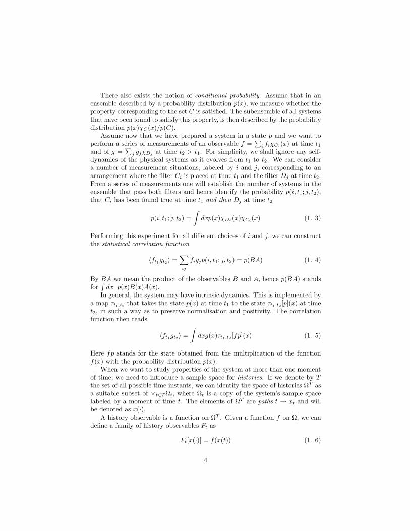
There also exists the notion of conditional probability: Assume that in anensemble described by a probability distribution p(x), we measure whether theproperty corresponding to the set C is satisfied. The subensemble of all systemsthat have been found to satisfy this property, is then described by the probabilitydistribution p(x)χC(x)/p(C).

Assume now that we have prepared a system in a state p and we want toperform a series of measurements of an observable f =

∑

i fiχCi(x) at time t1

and of g =∑

j gjχDjat time t2 > t1. For simplicity, we shall ignore any self-

dynamics of the physical systems as it evolves from t1 to t2. We can considera number of measurement situations, labeled by i and j, corresponding to anarrangement where the filter Ci is placed at time t1 and the filter Dj at time t2.From a series of measurements one will establish the number of systems in theensemble that pass both filters and hence identify the probability p(i, t1; j, t2),that Ci has been found true at time t1 and then Dj at time t2

p(i, t1; j, t2) =

∫

dxp(x)χDj(x)χCi

(x) (1. 3)

Performing this experiment for all different choices of i and j, we can constructthe statistical correlation function

〈ft1gt2〉 =∑

ij

figjp(i, t1; j, t2) = p(BA) (1. 4)

By BA we mean the product of the observables B and A, hence p(BA) standsfor

∫

dx p(x)B(x)A(x).In general, the system may have intrinsic dynamics. This is implemented by

a map τt1,t2 that takes the state p(x) at time t1 to the state τt1,t2 [p](x) at timet2, in such a way as to preserve normalisation and positivity. The correlationfunction then reads

〈ft1gt2〉 =

∫

dxg(x)τt1,t2 [fp](x) (1. 5)

Here fp stands for the state obtained from the multiplication of the functionf(x) with the probability distribution p(x).

When we want to study properties of the system at more than one momentof time, we need to introduce a sample space for histories. If we denote by Tthe set of all possible time instants, we can identify the space of histories ΩT asa suitable subset of ×t∈T Ωt, where Ωt is a copy of the system’s sample spacelabeled by a moment of time t. The elements of ΩT are paths t → xt and willbe denoted as x(·).

A history observable is a function on ΩT . Given a function f on Ω, we candefine a family of history observables Ft as

Ft[x(·)] = f(x(t)) (1. 6)

4

The state is represented by a probability measure P on ΩT . It containsinformation about both initial condition and the dynamics and for any functionF on ΩT it gives its mean value P (F ) or simply F . We can, abusingly, write itin terms of a probability distribution on ΩT

P (F ) =

∫

Dx(·)P [x(·)]F [x(·)] (1. 7)

The correlation functions 〈ft1gt2〉 can then be written as P (Ft1Gt2) in terms ofthe functions Ft and Gt defined by (1.6). The information of the correlationfunctions of a single observable f is contained in the generating functional

Zf [J(·)] =

∞∑

n=0

in

n!

∫

dt1 . . . dtn〈ft1 . . . ftn〉J(t1) . . . J(tn) =

∫

Dx(·)P [x(·)] exp

(

i

∫

dtFt[x(·)]J(t)

)

, (1. 8)

in terms of a function of time J(t), commonly referred to as the ”source”.The generating functional is essentially the Fourier transform of the proba-

bility measures. The definition can be extended for families of observables fi.Since correlation functions can be operationally determined, it is possible, inprinciple, to determine the probability measure with arbitrary accuracy.

1.3 Quantum correlations

In the previous section we gave a summary of classical probability theory, thusestablishing our notation, and identified the operational meaning of correlationfunctions in classical probability.

The corresponding structures for a single moment of time are well-knownin standard quantum theory. Elementary alternatives are rays on a complexHilbert space H , observables are self-adjoint operators on H , a general propertycorresponds to a projection operator and a state to a density matrix.

Let us now consider an ensemble of quantum systems prepared in a statedescribed by a density matrix ρ and try to operationally construct the correla-tion function of two observables A =

∑

aiPi and B =∑

j bjQj at times t1 and

t2 > t1 respectively. Here Pi refers to an exhaustive (∑

i Pi = 1 ) and exclusive

(PiPj = Piδij) set of projectors, and so does Qj .

Let the Hamiltonian of the system be H and ρ0 the state of the systemat time t = 0. Then a series of measurements will enable us to identify theprobability that Pi is found true and then Qj is found true. According to therules of quantum theory this will be

p(i, t1; j, t2) = Tr(

Qje−iH(t2−t1)Pie

−iHt1 ρ0eiHt1 Pie

iH(t2−t1))

=

Tr(

Qj(t2)Pi(t1)ρ0Pi(t1))

, (1. 9)

5

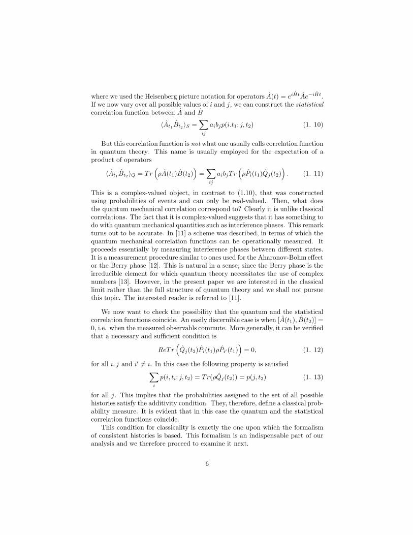
where we used the Heisenberg picture notation for operators A(t) = eiHtAe−iHt.If we now vary over all possible values of i and j, we can construct the statisticalcorrelation function between A and B

〈At1Bt2〉S =∑

ij

aibjp(i.t1; j, t2) (1. 10)

But this correlation function is not what one usually calls correlation functionin quantum theory. This name is usually employed for the expectation of aproduct of operators

〈At1Bt2〉Q = Tr(

ρA(t1)B(t2))

=∑

ij

aibjTr(

ρPi(t1)Qj(t2))

. (1. 11)

This is a complex-valued object, in contrast to (1.10), that was constructedusing probabilities of events and can only be real-valued. Then, what doesthe quantum mechanical correlation correspond to? Clearly it is unlike classicalcorrelations. The fact that it is complex-valued suggests that it has something todo with quantum mechanical quantities such as interference phases. This remarkturns out to be accurate. In [11] a scheme was described, in terms of which thequantum mechanical correlation functions can be operationally measured. Itproceeds essentially by measuring interference phases between different states.It is a measurement procedure similar to ones used for the Aharonov-Bohm effector the Berry phase [12]. This is natural in a sense, since the Berry phase is theirreducible element for which quantum theory necessitates the use of complexnumbers [13]. However, in the present paper we are interested in the classicallimit rather than the full structure of quantum theory and we shall not pursuethis topic. The interested reader is referred to [11].

We now want to check the possibility that the quantum and the statisticalcorrelation functions coincide. An easily discernible case is when [A(t1), B(t2)] =0, i.e. when the measured observabls commute. More generally, it can be verifiedthat a necessary and sufficient condition is

ReTr(

Qj(t2)Pi(t1)ρPi′(t1))

= 0, (1. 12)

for all i, j and i′ 6= i. In this case the following property is satisfied∑

i

p(i, ti; j, t2) = Tr(ρQj(t2)) = p(j, t2) (1. 13)

for all j. This implies that the probabilities assigned to the set of all possiblehistories satisfy the additivity condition. They, therefore, define a classical prob-ability measure. It is evident that in this case the quantum and the statisticalcorrelation functions coincide.

This condition for classicality is exactly the one upon which the formalismof consistent histories is based. This formalism is an indispensable part of ouranalysis and we therefore proceed to examine it next.

6

2 Quantum processes

2.1 Consistent histories

The consistent histories approach to quantum theory was developed by Griffiths[14], Omnes [4], Gell-Mann and Hartle [15, 5, 6]. The basic object is a history,which corresponds to properties of the physical system at successive instants oftime. A discrete-time history α will then correspond to a string Pt1 , Pt2 , . . . Ptn

of projectors, each labeled by an instant of time. From them, one can constructthe class operator

Cα = U †(t1)Pt1 U(t1) . . . U †(tn)PtnU(tn) (2. 1)

where U(s) = e−iHs is the time-evolution operator. The probability for therealisation of this history is

p(α) = Tr(

C†αρ0Cα

)

, (2. 2)

where ρ0 is the density matrix describing the system at time t = 0.But this expression does not define a probability measure in the space of all

histories, because the Kolmogorov additivity condition cannot be satisfied: if αand β are exclusive histories, and α∨β denotes their conjunction as propositions,then it is not true that

p(α ∨ β) = p(α) + p(β). (2. 3)

The histories formulation of quantum mechanics does not, therefore, enjoy thestatus of a genuine probability theory.

However, an additive probability measure is definable, when we restrict toparticular sets of histories. These are called consistent sets. They are moreconveniently defined through the introduction of a new object: the decoherencefunctional. This is a complex-valued function of a pair of histories given by

d(α, β) = Tr(

C†β ρ0Cα

)

. (2. 4)

A set of exclusive and exhaustive alternatives is called consistent, if for all pairsof different histories α and β, we have

Re d(α, β) = 0. (2. 5)

In that case one can use equation (2.2) to assign a probability measure to this set.The consistent histories interpretation then proceeds by postulating that anyprediction or retrodiction, we can make using probabilities, has always to makereference to a given consistent set. This leads to counter-intuitive situations,of getting mutually incompatible predictions, when reasoning within differentconsistent sets . The predictions of this theory are therefore contextual: but

7

in any case, this is a general feature of all realist interpretations of quantumtheory.

Except for trivial cases, it is only coarse-grained observables that satisfy anexact (or approximate) consistency condition. This means that the histories areconstructed out of projectors P , whose trace is much larger than unity.

2.2 The Closed-Time-Path generating functional

We saw that in quantum theories probabilities and statistical correlations arecontained in the decoherence functional; in fact, in its diagonal elements. Weshall now show that the same is true for the quantum correlation functions.

Recall that in the decoherence functional projectors enter in a time-orderedseries. This suggests that it would be best to use time-ordered correlationfunctions. Let Aa denote a family of commuting operators. Then the time-ordered two-point correlation function is defined as

G2,0(a1, t1; a2, t2) = θ(t2 − t1)Tr[ρ0Aa1(t1)A

a2(t2)] +

θ(t1 − t2)Tr[ρ0Aa2(t2)A

a1 (t1)]. (2. 6)

Here, we have denoted by θ(t) the step function.One can similarly define time-ordered n-point functions, or anti-time-ordered

G0,2(a1, t1; a2, t2) = θ(t1 − t2)Tr[ρ0Aa1(t1)A

a2(t2)] +

θ(t2 − t1)Tr[ρ0Aa2(t2)A

a1 (t1)] (2. 7)

In general, one can define mixed correlation functions Gr,s, with r time-orderedand s anti-time-ordered entries, as for instance

G2,1(a1, t1; a2, t2|b1, t′1) = θ(t2 − t1)Tr[Ab1 (t′1)ρ0A

a1(t1)Aa2(t2)] +

θ(t1 − t2)Tr[Ab1(t′1)ρ0Aa2(t2)A

a1 (t1)] (2. 8)

These correlation functions are generated by the Closed-Time-Path (CTP) gen-erating functional associated to the family Aa

ZA[J+, J−] =

∞∑

n,m=0

in(−i)m

n!m!

∫

dt1 . . . dtndt′1 . . . dt′m

Gn,m(a1, t1; . . . an, tn|b1, t′1; . . . ; bm, t′m)

Ja1

+ (t1) . . . Jan

+ (tn)Jb1− (t′1) . . . Jbm

− (t′m) (2. 9)

here Ja+ and Ja

− are functions of time, that play the role of sources, similar tothe ones in equation (1.8) for the classical stochastic processes.

The name closed-time arose, because in the original conception (by Schwinger[16] and Keldysh [17] the time path one follows is from some initial time t = 0

8

to t → ∞, thus covering all time-ordered points and then back from infinity to0 covering the anti-time-ordered points. The total time-path is in effect closed.

Conversely the correlation functions can be read from ZA

Gn,mA (a1, t1; . . . ; an, tn|b1, t

′1; . . . ; bm, t′m)

= (−i)nimδn

δJa1

+ (t1) . . . δJan

+ (tn)

δm

δJb1− (t1) . . . δJbm

− (tm)Z[J+, J−]|J+=J−=0.(2. 10)

2.3 Relation between the functionals

Clearly there must be a relation between the decoherence functional and theCTP one. One can see in the correlation functions, if we assume a singleoperator A =

∑

i aiPi and consider a pair of histories α(i1, t1; . . . ; in, tn) =

Pi1 , t1; . . . ; Pin, tn and β(i1, t

′1; . . . ; in, t′m) = Pj1 , t

′1; . . . ; Pjm

, tm. Then onecan easily verify that

Gn,mA (t1, . . . , tn; t′1, . . . , t

′m) =

∑

i1...in

∑

j1...jm

ai1 . . . ainbj1 . . . bjm

×d[α(i1, t1; . . . ; in, tn), β(j1, t1; . . . ; jm, tm)] (2. 11)

The straightforward relation is nonetheless not possible to show in an ele-mentary fashion. One needs to consider correlation functions at all times t andthis necessitates a description in terms of histories that can have temporal sup-port over the whole of the real line, or at least a continuous subset of it. Thiscan be achieved in the framework of continuous-time histories [18, 19, 20, 21].However, this requires a significant upgrading of the formalism of quantum me-chanical histories. The key idea is to represent histories by projectors on atensor product of Hilbert spaces ⊗t∈T Ht [22] in analogy to the construction ofthe history sample space classically. A suitable Hilbert space (not a genuine ten-sor product) can be constructed [18] for the case that T is a continuous set andthe decoherence functional can be defined as a bilinear, hermitian functional onthis space. It can then be shown that as a functional it is essentially a double”Fourier transform” of the CTP generating functional.

This proof is to be found in [10] and is elementary once one follows the logicof the construction. Here we shall restrict ourselves to a convenient statementof this result.

Let us assume that we have a family of commuting self-adjoint operators Ai.Their spectrum is then a subset Ω of some vector space Rn. Any operator thatcommutes with Ai is in one-to-one correspondence to functions f(x) with x ∈ Ωand can be written as f(A). Like the classical case we can construct a space ofhistories ΩT as a suitable subset of ×t∈T Ωt. Subsets of of ΩT are histories ofthe quantum mechanical observables Ai.

The decoherence functional is then a map that to each pair of subsets Cand C′ of ΩT it assigns a complex number in such a fashion that the following

9

properties are satisfied [6, 23]

- d(C′, C) = d∗(C, C′), hermiticity- d(0, C) = 0, null triviality- d(1, 1) = 1, normalisation- d(C ∪ C′, D) = d(C, D) + d(C′, D) for disjoint C and C′, additivity.

Such a decoherence functional can be constructed as a continuum-limit of thediscrete-time expressions (2.2). Because of the additivity condition, one canformally write the decoherence functional as an integral over ΩT × ΩT

d(C, D) =

∫

Dx(·)Dx′(·) ∆[x(·)|x′(·)] χC [x(·)]χD [x′(·)], (2. 12)

in terms of a function D : ΩT ×ΩT , that plays the role of an integration kernel.This is in complete analogy to the stochastic probability measure P [x(·)] ofequation (1.7).

One can view ∆[x(·)|x′(·)] as the decoherence functional between a pair offine-grained histories x(·) and x′(·), only that such histories cannot be repre-sented by projectors on a Hilbert space. For example, if these histories wheredefined on the configuration space for the time interval [ti, tf ], one could writethe standard expression [6]

∆[x(·)|x′(·)] = ρ0[x(ti), x′(tf )]δ[x(tf ), x′(tf )] eiS[x(·)]−iS[x′(·0], (2. 13)

in terms of the matrix elements of the initial density matrix ρ0, the standardconfiguration space action and a delta-funtion for the final-time points of thepaths.

If ZA[J+, J−] is the CTP generating functional associated to Ai we have

ZA[J+, J−] =

∫

Dx(·)Dx′(·)ei∫

dtJa+(t)xa(t)e−i

∫

dtJa−

(t)x′a(t)∆[x(·)|x′(·)](2. 14)

In other words viewed as a bi-functional over the functions on ΩT the deco-herence functional is identical to the CTP generating functional. The onlydifference is on the type of functions upon which they take values - the first oncharacteristic functions, the second on complex valued functions of unit norm.In fact, equation (2.12) amounts to

Gn,m(a1, t1; . . . ; an, tn|b1, t1; . . . ; bm, tm) =

∫ ∫

Dx(·)Dx′(·)

×xa1(t1) . . . xan(tn)x′b1 (t′1)x′bm (tm)∆[x(·)|x′(·)] (2. 15)

Hence there exists the following correspondence between classical and quan-tum probability

10

Quantum → ClassicalProbabilities d(C, C′) → p(C)Correlations Z[J+, J−] → Zcl[J ]

The probability measure is a real-valued functional on functions of ΩT , whilethe decoherence functional is a hermitian bilinear functional on the functions ofΩT . In a given system, one goes from d to p, when the decoherence condition(2.5) is satisfied, while in both cases one goes from probabilities to correlationsthrough a Fourier transform.

What we will next show is how to effect the transition from the CTP generat-ing functional to a stochastic process for the coarse-grained variables. Workingat the level of the correlation functions makes the construction of stochasticdifferential equations easier than working at the level of probabilities.

3 From quantum to classical

3.1 The basic choice for coarse graining

In order to study the transition from quantum to classical, we need to choosethe variables, upon which we shall concentrate. This amounts to a choice ofa family Ai of intercommuting operators. Now, a maximal family of intercom-muting operators generically contains full information about the evolution ofthe quantum system. (Possible exceptions to this rule are trivial cases, as, forinstance, when the Hamiltonian and the initial density matrix commutes withall Ai).

One can implement a coarse-graining procedure even at this stage. It suf-fices to take for Ai a non-maximal family of operators. This is the case, forinstance, in quantum Brownian motion models. If we assume that the totalsystem consists of a large number of harmonic oscillators, a maximal familyof intercommuting operators consists of the position operators of all particles.When we choose to focus on a single one of them, we effectively coarse-grain bytreating the remaining degrees of freedom as an environment. This is the type ofcoarse-graining associated with the studies of environment-induced decoherence.

However, this type of coarse-graining does not suffice. One has usually toconsider smeared values of the relevant observables. This is effected by consid-ering projectors, which are sufficiently smeared over Ω. We shall take Ω to beRs so its points will be vectors xa.

In general, it is difficult to work with characteristic functions, so we willwork with smeared characteristic functions. If we denote by |x| their Euclidean

11

distance, then a good choice for the projector is the function

fx(x) = exp(− 1

2σ2|x − x|2) (3. 1)

This Gaussian is not a sharp projector; it is strongly peaked in a sphere of lengthσ around the point x, hence it is a good approximation to a true projector fornot very large values of σ.

We can construct discrete-time histories, consisting of projectors fxticen-

tered around xti, at each time ti . One such history can be viewed as a discretised

approximation to a coarse-grained history in continuous-time, centered arounda path t → x(t).

We now consider two such discretised histories, centered at the same timepoints ti each corresponding to a different path x(·) and x′(·). Let us denotethem by αx(·) and αx′(·). If we expect our system to exhibit classical behaviour,then the off-diagonal elements of the decoherence functional will fall rapidly,whenever δ2 = ||x(·) − x′(·)||2 :=

∑

i |xti− x′(ti)|2 is much larger than N × σ2.

(Here N is the number of time-steps). Typically one has

d(αx(·), αx′(·)) = O(e−δ2/Nσ2

), (3. 2)

or some other type of rapid fall-off. For pure initial states, this behaviour isexpected, when σ2 much larger than the uncertainties of the initial state andthe Hamiltonian evolution preserves this property [24]. In this case, the diagonalelements are close to defining probabilities for coarse-grained histories centeredaround x(·) and with a spread σ at each moment of time.

Now, we want to find a probability distribution that would give these valuesfor the probabilities of these histories. A single-time projector is centered in avolume of Ω of size

∫

dxfx(x) = (2πσ2)r/2. (3. 3)

A probability distribution on the space of (discretised) paths that reproducesthese expressions for probabilities of these coarse grained sets is

p[x(·)] =1

(2πσ2)rn/2d(αx(·), αx(·)), (3. 4)

where n is the number of time-steps assumed. (Dividing by the volume turnsthe probabilities of events into a density.)

One can use equation (2.12) to write

d(αx(·), αx(·)) =

∫

Dx(·)Dx′(·)

× exp(− 1

2σ2||x(·) − x(·)||2 − 1

2σ2||x′(·) − x(·)||2)∆[x(·)|x′(·)] (3. 5)

12

Note that our expressions are still defined with respect to discrete time.From equation (2.13) we see that the kernel ∆ can be obtained from the

inverse Fourier transform of the CTP generating functional. This yields

p[x(·)] =

∫

DJ+(·)DJ−(·)e−1/4π(J+·J++J−·J−)−i/√

2πx·(J+−J−)

×Z[J+/(√

2πσ), J−/(√

2πσ)] (3. 6)

There is now no multiplicative term, that depends on the number of timesteps. Hence, one can safely go to the continuum limit from this expression. Wehave denoted as J ·x =

∑

i J(ti)x(ti) and at the continuum limit this expressionwill become an integral.

To get the generating functional for the classical correlation functions oneFourier transforms the probability measure to get (we now drop the index thatrefers to our choice of variables for the correlation functions)

Zcl[J ] = e−σ2

8J·J

∫

dR(·)e−1/2πR·RZ[R√2πσ

+J

2,

R√2πσ

− J

2], (3. 7)

with R = 12 (J+ + J−).

This generating functional needs to be normalised to unity by assuming thatZcl[0] = 1. The normalisation condition is not kept, because we have employedapproximate characteristic functions. Had we used a sharp characteristic func-tion, the construction would automatically guarantee normalisation. Now thereis a deviation from unity of the order of σ2.

The expression (3.7) can be simplified. Assume that we have a classicalstochastic process for the variables x(·), with a generating functional Z0[J ]. Letus follow the same procedure for coarse-graining as before, using the approxi-mate projectors (3.1). The coarse-grained generating functional would be

Zcl[J ] = e−σ2

2J·JZ0[J ] (3. 8)

This means, that we can consider the generating functional in equation (3.7)as coming from coarse-graining a classical stochastic process, with twice thedegree of coarse graining as the one from quantum theory. One can then dropthe term outside the integral in (3.7) as coming from coarse-graining of anunderlying stochastic process given by

Zcl[J ] =

∫

dR(·)e−1/2πR·RZ[R√2πσ

+J

2,

R√2πσ

− J

2] (3. 9)

This equation gives the stochastic correlation functions in the classical limitof the quantum system described by the CTP generating functional Z[J+, Z−].It should be always kept in mind, that this process gives reliable results only onscales much larger than σ2.

13

We should now pause for a minute and examine the assumptions we used inorder to arrive here.

First, one should ask what is the meaning of the parameter σ. Is it arbi-trary or not? In principle it is not. It is the degree of coarse-graining, thatis necessary in order that the fall-off (2.5) of the off-diagonal elements of thedecoherence functional is manifested. It, therefore, has to be much larger thanthe natural scale associated with microscopic processes; however, it ought to besmall compared to macroscopic scales.

In principle, σ can be determined from a full study of the decoherence func-tional. Usually a measure of coarse-graining is the trace of the correspondingpositive operator. However, we have here considered only commuting variableswith continuous spectrum and the trace of the operators corresponding to (3.7)is infinite. This is related to the fact that there is no default universal scale,by which to judge whether σ is large. This problem is remedied by consideringphase space coarse-grainings as we shall see shortly. In this case the naturalscale is h = 1 and one can say that σ2 >> 1 in order to have consistency ofhistories. It should nonetheless be much smaller than a macroscopic time scaleby which we observe phenomena.

More precisely , the stochastic approximation (3.9) is accurate within anorder of (lmic/σ)2, where lmic is the microscopic scale that is determined by thedynamics or the initial state. However, there is also an error proportional to(σ/Lmac)

2, where Lmac is the macroscopic scale of observation, i.e. the scaleof accuracy we are interested in having. This is due to the use of the Gaussianapproximation for the projectors. Overall we have an error of the order of

c1(lmic/σ)2 + c2(σ/Lmac)2, (3. 10)

where c1 and c2 are constants of the order of unity. It is, therefore, evident thata separation of scales is necessary, if the stochastic description is to make anysense.

Second, the general logic of this construction is to identify a stochastic pro-cess that adequately describes the evolution of the classicalised coarse-grainedobservables. There is a subtle difference from the consistent histories scheme,in that we do not seek to construct consistent sets for the system and hencemake statements about individual quantum systems. Our approach is more op-erational. Given that quantum theory is a model that provides the statisticalbehaviour of physical systems, we ask to construct a different model based onprobability theory that describes some regime of the same physical system. Forthis purpose we utilise the consistency condition in order to identify the valid-ity of our approximation. Then, we build the probability distribution from thediagonal elements of the decoherence functional.

14

3.2 Phase space coarse grainings

One does not have to restrict to correlation functions of a family of commutingoperators in order to construct the CTP generating functional. By consideringcorrelation functions in both position and momentum, it is possible to generalisethe definition (2.9). Indeed in this equation it is not necessary to assume that theoperators Aa are commuting. We assumed commutativity, because we wanteda description in terms of paths on the common spectrum of these operators.

However, in any Hilbert space, that carries a representation of the canonicalcommutation relations

[qi, pj ] = iδij (3. 11)

it is possible to assign a function on the phase space Γ = (qi, pi) for eachoperator by means of the Wigner transform

A → FA(q, p) =

∫

dξdχe−iqξ−ipχTr(

Aeiqξ+ipχ)

:= Tr(

A∆(q, p))

(3. 12)

An important property of this transform is that it preserves the trace:

TrA =

∫

dqdpFA(q, p) (3. 13)

However, the Wigner transform does not preserve multiplication of operators.The defining condition P 2 = P for projectors is therefore not preserved and aprojector is mapped into some general positive function, rather than a charac-teristic function of a subset of Γ.

Since any operator can be represented by a function of Ω, histories wouldbe represented by functions on a space ΓT , which will be a suitable subspaceof ×t∈T Γt. In reference [10] it was shown that a decoherence functional canbe constructed as an hermitian bilinear functional on the space of functions onΓT . And it is related to the CTP generating functional by means of a Fouriertransform.

All the formulas in the previous paragraph can then be reinterpreted to fitthe phase space context, by allowing the variables x to denote both q and p.(The dimension of Γ is clearly even). The main difference is that the Gaussianfunction fx corresponds to an operator F with a finite trace. By virtue of (2.1)and (2.13)

TrF = (2πσ2)r/2 (3. 14)

The parameter σ has units of action and is an absolute measure of the degree ofcoarse-graining on phase space. Consistency occurs whenever σ2 >> h, whereh provides the natural length scale on phase space. In fact, in the study, ofa large class of closed quantum systems, Omnes has showed [25] that the off-diagonal elements of the decoherence functional are of the order of (h/σ)r/4,where r = 2k is the dimension of Γ. Hence, even if h/σ ∼ 10−8 there isa substantial degree of decoherence to justify the use of classical probability

15

and σ is still sufficiently small compared to some external macroscopic scalesto justify the use of the Gaussian approximation for the projector. From amacroscopic perspective it would be sufficient to consider the leading order inσ2 of the correlation functions.

The study of phase space histories is more intricate, because one has tochoose proper units for position and momentum, by which to write Euclideannorm in the coarse-grained projector (2.1). For classicality it is not only neces-sary to have a large value of σ, but the choice of units has to be preserved by thedynamical evolution [25, 26]. This is a non-trivial condition that largely dependson the system’s Hamiltonian. For this we shall prefer to employ configurationspace coarse-grainings.

Whenever we have a representation of the canonical commutation relationswe can define the coherent states

|z〉 = |χξ〉 = eiqξ+ipχ|0〉, (3. 15)

where |0〉 is a fiducial vector, often taken to be the lowest energy eigenstate.The important point is that one can assign to a large class of density matricesρ a function fρ(χ, ξ) (its P-symbol) defined by

ρ =

∫

dχdξf(χ, ξ)|χξ〉〈χξ|. (3. 16)

If one then denotes by Zχ0ξ0[J+, J−] the CTP generating functional corre-

sponding to an initial state given by |χ0ξ0〉 then the CTP generating functionalfor the same system but a different initial state ρ

Z[J+, Z−] =

∫

dχ0dξ0fρ(χ0, ξ0)Zχ0ξ0[J+, J−] (3. 17)

and a similar equation would hold for the classical limit, provided that thedegree of coarse-graining necessary for decoherence is determined by the studyof the state ρ rather than the coherent states.

3.3 Gaussian processes

Let us now consider a quantum system described by a Gaussian CTP generatingfunctional. Its most general form would be

Z[J+, J−] = exp

(

− i

2J+ · L · J+ +

i

2J− · L · J−

+iJ+ · K · J− + i(J+ − J−) · X) (3. 18)

Here we have denoted by L kernels of the form Lab(t, t′), by J · L · J ′ =∫

dtdt′Ja(t)Lab(t, t′)Jb(t′) and the bar denotes complex conjugation. X denotes

16

the one-point function G10 = G01 and

iLab(t, t′) = G2,0(a, t; b, t′) − X(a, t)X(b, t′) (3. 19)

iKab(t, t′) = G1,1(a, t|b, t′) + G1,1(b, t′|a, t) − 2X(a, t)X(b, t′) (3. 20)

We can write L = L1 − iL2 and K = K1 − iK2, in terms of the real-valued kernels L1, L2, K1, K2. The hermiticity condition on the CTP generatingfunctional would then entail

LT1 = L1 LT

2 = L2 (3. 21)

K1 = 0 K2 = 2L2 (3. 22)

Evaluating the integral (3.7) yields

Zcl[J ] = e−J·Ξ·J+iJ·X (3. 23)

where

Ξ = L2 +1

4σ2L1 · L1 (3. 24)

It is worth noticing, that whenever the term L2 is dominant, the classicaltwo-point function is independent of the coarse-graining scale and equal to thereal part of the quantum two-point function. However, this simplification canoccur only in Gaussian systems.

4 Examples

4.1 Harmonic oscillators

For a single harmonic oscillator with frequency ω and mass m in a thermal state,we have for the configuration space correlation functions

L1(t, t′) = − 1

2mωsin ω|t − t′| (4. 1)

L2(t, t′) =

1

2mωcoth(βω/2) cosω(t − t′) (4. 2)

(4. 3)

and equation (3.24) gives Ξ(t, t′).One should recall that the smearing scale σ is determined by the condition

(2.5) on the fall-off of the diagonal elements of the decoherence functional. Hereσ2 should be much larger than (2mω)−1, the position uncertainty of the groundstate. This can be verified by direct evaluation, but it is made plausible by thefollowing observation: a thermal state has a positive P-symbol, and hence itsquantum behaviour is identical to the one of the coherent states, which in aGaussian system is identical with that of the vacuum.

17

The term L1 · L1 is proportional to (σ2mω)−1, hence comparatively small.In particular, at high temperature βω << 1 the L2 term is dominant, thecorrelation function is σ-independent and one recovers the classical result.

Let us recall that this system does not describe a harmonic oscillator incontact with a heat bath; it describes a closed system, evolving unitarily andprepared in a thermal state (whatever that might mean). Physically more rel-evant is the case of an oscillator undergoing quantum Brownian motion, to betaken up later.

But we shall first examine the case, where the system is initially prepared ina squeezed state. A squeezed state |r, φ〉 is the zero eigenstate of the operator

b = cosh r/2a + sinh r/2eiφa†, (4. 4)

where r ≥ 0. The correlation function L1 is identical to the one for the vacuumcase, while

L2(t, t′) =

1

2mω(cosh r cosω(t − t′) + sinh r cosω(t + t′ − φ)) (4. 5)

Clearly it is necessary that σ2 >> cosh r2mω in order to have decoherence. In

that case the L21 term is again negligible. For values of r at the order of unity,

it is not different from the vacuum case, but for large r the degree of coarse-graining necessary for classicality might become too large to allow us to obtainany useful information. This is what is meant, when we say that squeezed statesare highly non-classical states.

4.2 Quantum Brownian motion

We shall study here the Caldeira-Leggett model [27, 28, 29], i.e. a single har-monic oscillator of mass M and frequency ω coupled linearly to a bath of har-monic oscillators in a thermal state. More precisely the system is defined by theHamiltonian

H =p2

2M+

1

2Mω2x2 + x

∑

i

ciqi +∑

i

(p2

i

2mi+

1

2miω

2i q2

i ). (4. 6)

From the Heisenberg equations of motion we get

Md2

dt2x + Mω2x2 = −

∑

i

ciqi, (4. 7)

d2

dt2qi + ω2

i q2i = − ci

mix. (4. 8)

The second equation has a solution

qi(t) = q0i cosωit +p0i

miωisinωit −

ci

miωi

∫ t

0

ds sin ωi(s − s′)x(s), (4. 9)

18

which when substituted into (4.7) yields

d2

dt2x + ω2x − 2

M

∫ t

0

dsη(t − s)x(s) = − 1

M

∑

i

ciqi(t) (4. 10)

Here

η(s) =∑

i

c2i

2miωisin ωis, (4. 11)

is known as the dissipation kernel. Let us denote by u(t) the solution of thehomogeneous equation corresponding to (4.10) with the initial conditions u(0) =1 and u(0) = 0. It can be identified as the inverse Laplace transform of thefunction

u(s) =1

s2 + ω2 − 2/Mη(s), (4. 12)

where η is the Laplace transform of the dissipation kernel. We can then writethe solution of (4.10) as

x(t) = x0u(t) +p0

Mu(t)

− 1

M

∑

i

ci[q0i

∫ t

0

dsu(t − s) cosωis +p0i

miωi

∫ t

0

dsu(t − s) sin ωis] (4. 13)

Now we assume that the initial state of the system is factorisable to a thermalstate at temperature T = β−1 for the environment and a density matrix ρ0 forthe distinguished oscillator. In this case, we can easily see that the expectationvalue

x(t) = Tr[ρ0x(t)] = x0u(t) +p0

Mu(t), (4. 14)

is a solution of the dissipative equations of motion , while the two-point functionreads

Tr[ρ0x(t)x(t′)] = (∆x0)2u(t)u(t′) +

(∆p0)2

M2u(t)u(t′) +

Cpq

M[u(t)u(t′) + u(t′)u(t)] +

i

2M[u(t)u(t′) − u(t′)u(t)]

+1

M2[

∫ t

0

ds

∫ t′

0

ds′u(s)ν(s − s′)u(s′) + i

∫ t

0

ds

∫ t′

0

ds′u(s)η(s − s′)u(s′)](4. 15)

Here ∆x0, ∆p0 and Cpq are the uncertainties and correlation between positionand momenta at t = 0. Also,

ν(s) =∑

i

c2i

2miωicoth

βωi

2cosωis (4. 16)

is known as the noise kernel.

19

From this equation, it is easy to determine the kernels L and K. If we writethe last line in equation (4.15) as 1

M2 [N(t, t′) + iH(t, t′)] we have

L1(t, t′) = θ(t − t′)[

1

M[u(t)u(t′) − u(t′)u(t)] +

1

M2H(t, t′)]

+θ(t′ − t)[1

M[u(t′)u(t) − u(t)u(t′)] +

1

M2H(t′, t)] (4. 17)

L2(t, t′) = (∆x0)

2u(t)u(t′) +(∆p0)

2

M2u(t)u(t′)

+Cpq

M[u(t)u(t′) + u(t′)u(t)] +

1

M2N(t, t′) (4. 18)

Now we want to derive the stochastic limit, to which these quantum corre-lation functions correspond. We shall use equation (3.24). Note however, thatthe necessary degree of coarse-graining in order to achieve decoherence must bein a phase space region much larger than the one occupied by the initial state.Hence we take the coarse-graining scale to be much larger than the uncertaintiesand correlations of the initial state. This allows us to drop all terms but N(t, t′)in equation (4.15). The semiclassical equations are then largely independent ofthe details of the initial state.

To see this in more detail we need to specify a given distribution of modesand couplings in the environment. This information is encoded in the spectraldensity

I(k) =∑

i

c2i

2miωiδ(k − ωi) (4. 19)

If the spectral density is specified, then we can fully determine the noise anddissipation kernels as

η(s) =

∫

dkI(k) sin ks (4. 20)

ν(s) =

∫

dkI(k) coth(βk

2) cos ks. (4. 21)

A large class of physically interesting choices for spectral density are

I(k) =2Mγ

πk

(

k

Θ

)s−1

, k ≤ Λ

0 , k > Λ, (4. 22)

where Λ is a high-frequency cut-off. The exponent s determines the infra-redbehaviour of the bath. For s = 1 the environment is called ohmic, for s < 1subohmic and for s > 1 supraohmic.

20

High temperature For high temperature βΛ << 1, the L2 term is pro-portional to β−1 and dominates the classical correlation function. The classi-cal stochastic process will be then independent of the precise choice of coarse-graining. The two point function for x will then be

Ξ(t, t′) =1

M2

∫ t

0

dsu(t − s)

∫ t′

0

ds′u(t′ − s′)ν(s − s′) (4. 23)

But this is the correlation function for the solution of the classical stochasticdifferential equation

Md2

dt2x(t) + Mω2x(t) −

∫ t

0

dsη(t − s)x(s) = f(t), (4. 24)

where f(t) is a Gaussian process with two-point function

〈f(t)f(t′)〉 = η(t − t′). (4. 25)

The noise kernel then gives the correlation function for an external noise per-turbing the classical dissipative equations of motion. This justifies its name andrecover results suggested by path integral techniques [28], or explicitly provedonly in particular regimes [6, 24]. Note, however, that this is true only whenthe L2 term in (3.24) dominates, as is the case of high temperature. In theprevious paragraph it is by necessity that the L‘21 term is small. Here it is notthe case, because L1 contains also a contribution from the environment degreesof freedom that might give a substantial contribution in certain regimes. In thegeneral case the L2

1 term might be of importance, something that implies thatthe stochastic limit will not be given by such a simple expression in terms of anexternal force guided by the noise kernel.

4.3 Scalar field

Consider now the case of a free, massive scalar field in vacuum. The correlationfunctions read

L1(x, t;x′, t′) = −∫

d3k

(2π)31

2ωk

e−ik·x sin ωk|t − t′| (4. 26)

L2(x, t;x′, t′) = −∫

d3k

(2π)31

2ωk

e−ik·x cosωk(t − t′) (4. 27)

Since ωk ≥ m, coarse-grainings with σ2m2 >> 1 for each mode will manifest asuppression of the interferences. As in the harmonic oscillator the L2

1 term, willbe negligible and the L2 will provide the classical correlation function.

For a massless field, there is no natural coarse-graining scale for all modes.One needs to take larger values of σ to adequately deal with the infra-red modes.

21

Configuration space coarse-graining is clearly bad in such a case. The analysishas to be performed in phase space and provides the same results as the m 6= 0case [30].

Consider now the case of a free scalar field in a general globally hyperbolicspacetime. The reader is referred to the standard treatments of Birrell andDavies [31] and Wald [32]. Let us by t denote the time coordinate in a spacelikefoliation, by x the spatial coordinates and let us use a collective index α to labelthe modes. The Heisenberg-picture field will read then

φ(x, t) =∑

α

[

aαuα(x, t) + a†αuα(x, t)

]

, (4. 28)

where uα(x, t) are some complex-valued solutions to the Klein-Gordon equationand

[aα, a†β] = δαβ . (4. 29)

Let us assume that the system is found in a Gaussian state |Ω〉, which isannihilated by the operator aα. The action of a† on |Ω〉 produces all states ofthe Fock space. It is easy to compute

〈Ω|φ(x, t)φ(x′, t′)|Ω〉 =∑

α

uα(x′, t′)uα(x, t) (4. 30)

Let us now consider a particular instant t = 0 as reference time, in whichthe mode functions u0

α(x) = uα(x, t) form an orthonormal basis

∫

dxu0α(x)u0

β(x) = δαβ (4. 31)

∫

dxu0α(x)u0

β(x) = 0. (4. 32)

Here, we wrote as dx the volume element of the push-backed spacetime metricin the spacelike surface t = 0. Any scalar function on a instant of time can bedecomposed in modes

uα(x, t) = Aαβ(t)u0β(x) + Bαβ(t)u0

β(x) (4. 33)

The matrices A and B are the Bogolubov coefficients and satisfy the matrixidentity

A†A − B†B = 1, (4. 34)

which essentially means that time evolution is given (classically) by a symplectictransformation. The correlation function (4.30) reads then

〈Ω|φ(x, t)φ(x′, t′)|Ω〉 =

u0(x′)A†(t′)A(t)u0(x) + u0(x′)B†(t′)B(t)u0(x)

+u0(x′)A†(t′)B(t)u0(x) + u0(x′)B†(t′)A(t)u0(x), (4. 35)

22

where a matrix notation has been employed.This gives for the kernels

L1(t,x; t′,x′) = −2θ(t − t′) Im u0(x′)[A†(t′)A(t) − B†(t′)B(t)]u0(x)

− 2θ(t′ − t) Im u0(x)[A†(t)A(t′) − B†(t)B(t′)]u0(x′)(4. 36)

L2((t,x; t′,x′) = 2 Re u0(x′)[A†(t′)A(t) + B†(t′)B(t)]u0(x)

+ 2 Re u0(x′)A†(t′)B(t)u0(x) (4. 37)

The Bogolubov transformation is a generalisation of the squeezing transfor-mation we studied earlier. For a single mode we had to coarse-grain in regions ofconfiguration space much larger than the uncertainty. It is similar in this case.We can coarse-grain each mode separately at a scale σ2. From equation (4.35)we can read the uncertainty for each mode (defined using the mode functionsu0

α). This will be equal to

(∆φα)2 = [A†A + B†B]αα(t) + [A†B + B†A]αα(t) (4. 38)

The first term is always larger in norm than the second due to Schwarzinequality. The degree of coarse-graining in each mode must be much largerthan (A†A + B†B)αα(t) for all t. To have a uniform coarse-graining scale forall modes it is necessary that σ2 has to be much larger than the norm of thematrix

||A†A + B†B||(t) = ||2A†A − 1||(t) < 2||A||2(t) (4. 39)

The matrix A has a finite norm be virtue of the Bogolubov identity (4.34). Now,in order to have a meaningful coarse-graining procedure it is necessary that thenorms of the Bogolubov matrices must be bounded in time. Hence one canwrite a sufficient condition for the possibility of a coarse-graining scale σ2 validfor all modes is that

σ2 >> supt

||A(t)||2 (4. 40)

We can then employ equation (3.24) to identify the correlation function for theclassicalised field. Due to (4.40) the L2

1 term will in general be smaller, as in thecase of the squeezed system hence the distribution (4.37) gives the correlationfunction of the classical stochastic process.

4.4 Perturbative expansion

So far we have considered only the case of Gaussian processes. We shall nowstudy the case of non-quadratic systems through the use of perturbation theory.Let us by Z0[J+, J−] denote a CTP generating functional that can be exactlyevaluated, e.g. a Gaussian. In general, a perturbative expansion around Z0 willbe of the form

Z[J+, J−] = exp

(

iF [iδ

δJ+,−i

δ

δJ−]

)

Z[J+, J−], (4. 41)

23

in terms of a functional F [x(·), x′(·)], that depends on some coupling constant.In the case that the CTP generating functional depends on configuration spacevariables, the Hamiltonian is of the form H0 + V (x) and the initial state is thevacuum, then we have

Z[J+, J−] = exp

(

i

∫

dtV [iδ

δJ+(t)] − iV [−i

δ

δJ−(t)]

)

Z0[J+, J−] (4. 42)

Substituting J± = R/(√

2πσ) ± J/2 in equations (4.42) yields for the classicalgenerating functional

Zcl[J ] =

∫

dR(·)e− 12π

R·R

exp

(

i

∫

dt(V [i

2

δ

δJ(t)+ i

√

π/2σδ

δR(t)]

−V [i

2

δ

δJ(t)+ i

√

π/2σδ

δR(t)])

)

Z0[R√2πσ

+J

2,

R√2πσ

− J

2] (4. 43)

If we assume that the length scale by which the potential varies is much largerthan σ we can keep the lower order term in σ in the exponential to get

Zcl[J ] =

∫

dR(·)e− 12π

R·R

× exp

(

−∫

dt√

π/2σV ′[i

2

δ

δJ(t)]

δ

δR(t)

)

Z0[R, J ]

≃ Zcl0 [J ] −

∫

dt1

2√

2πσV ′[

i

2

δ

δJ(t)]

∫

dR(t)R(t)e−14π

R·RZ0[R, J ], (4. 44)

where Z0[J ] is defined from Z0[J+, J−] via (3.9) and we wrote for brevityZ0[R, J ] = Z0[R/

√2πσ + J/2, R/

√2πσ − J/2].

The above expression is the leading order in σ of the generating functionaland is valid only when the potential V is assumed to vary in macroscopic scales.

Note, that as we see from (4.44), a perturbation expansion of the quan-tum theory does not generically amount to a perturbative expansion in thecorresponding classical limit. These results are of relevance for the study ofperturbation theory in quantum Brownian motion [33, 34].

5 Concluding remarks

Let us now summarise our results. We first showed that the quantum mechanicalcorrelation functions do not correspond to the statistical properties of a physicalsystem and hence do not correspond to a classical stochastic process. Then weexplained the relation of Schwinger and Keldysh’s CTP generating functionalto the decoherence functional of the consistent histories approach to quantum

24

theory. This enabled us to use the decoherence condition for histories in orderto develop a procedure of going from a quantum process to a stochastic processthat corresponds to a given degree of coarse-graining for a class of observables.The end result was equation (3.9) that gives the relation between the classicalgenerating functional and the CTP generating functional. But we should keepin mind that any results of the stochastic description that give some detailedstructure in scales smaller than σ are unreliable.

We then proceeded to study examples. We showed that in Gaussian pro-cesses the classical limit is a Gaussian process, with a correlation function givenby the real part of the quantum two-point function plus a term that dependson the coarse-graining scale. The second term is negligible in general, but thisis not necessary in the case of quantum Brownian motion at low temperatures,because then it largely depends on properties of the bath, rather than the initialcondition of the distinguished system.

Now, what is the use of these results? The answer is that a stochasticdescription might be more amenable to our intuition than a quantum one. Forinstance, given a stochastic process, one can simulate the evolution of individualsystems and identify typical behaviours. This is something that cannot be donein quantum theory. We have no (uncontroversial) way to describe the randomevolution of an individual system’s observables, while in classical probabilitywe can write equations of the Langevin type. In this sense, the stochasticapproximation captures an aspect of the quantum mechanical randomness thatmight be manifested on macroscopic or even intermediate scales. Hence forBrownian particle, the knowledge of the noise due to the environment might besufficient for certain applications.

Substituting the full quantum behaviour for an approximate description interms of Langevin equation is necessary in cases, where the quantum system actsas a driving force term for another classical one. This is the case, for instance,of any detector coupled to a quantum field. While one often uses a quantumdescription for a detector, this is clearly inappropriate for realistic systems: adetector is a macroscopic system and the description of its effective behaviour interms of a simple Schrodinger equation is an idealisation that is hardly justifiedfrom first principles. On the other hand a detector can be treated as a classicalsystem - e.g. with respect to its center of mass- that is coupled to a stochasticdriving force, that arises from the fluctuation of the quantum system, with whichit is coupled. In this case the stochastic description of a quantum system is notonly convenient, but necessary.

The situation is similar in the case of quantum field theory in curved space-time as far as the issue of backreaction is concerned. The quantum field actsas a source for the classical gravitational field via its stress-energy tensor. Onewrites then the semiclassical gravity equation

Gµν = κ〈Tµν〉 (5. 1)

25

There is an underlying assumption in any use of this equation. As it stands itis nonsensical: on the left hand side is an observable for an individual systemand on the right hand side an ensemble average. What is implied is that i) thebehaviour of the quantum field is in some regime approximately deterministicand ii) the corresponding classical value of the stress energy tensor is equal tothe expectation value over the field’s state.

Of course these two assumptions need to be verified. In order for the quan-tum field to behave classically, coarse-graining is necessary. Even with coarse-graining it is not necessary that the system will classicalise. For instance, inthe one-dimensional case, time evolution might cause a continuous increase ofthe squeeze parameter in a given mode. In this case no fixed degree of coarse-graining is good at all times and it is very little we can do with a classicaldescription. Let us assume, however, that this is not the case. According toour earlier analysis, this would mean that we can choose a coarse-graining scalesatisfying equation (4.40). Then, one might expect that the system will exhibitstochastic behaviour for at least some of its properties.

In order for assumption i) to be valid, the stochastic process for the stress-energy tensor should have small deviations from its mean. This is rarely true, asin simple spacetimes one can show that the quantum fluctuations of the stress-energy tensor are of the same order of magnitude as its mean value [35]. Thisleads to the point that the semiclassical description of backreaction of quantumfields onto geometry ought to have a stochastic component [36, 37, 38, 39, 40,41, 42].

This is where our results in section 4.3 are of relevance. First, we arguedthat the condition (4.40) is sufficient to obtain classicality; then we showed thatit is essentially the real part of the two-point function of the fields that givesthe two-point function at the classical limit. Now the stress energy tensor is aquadratic functional of the fields

T µν(x) =1

2∇µφ(x)∇νφ(x) − 1

2gµνφ(x)(−∇ρ∇ρ + m2)φ(x) (5. 2)

Its expectation value can be read from the two-point function via pointsplitting and renormalisation. This means that we can define

〈T µν(x)〉 = limx′→x

1

2[1/2(∇µ

x∇νx′ + ∇µ

x∇νx′)

−1/2[gµν(x) + gµν(x′)](∇ρx∇x′ρ + m2)∆2(x, x′) (5. 3)

Now, the imaginary point of the two point function vanishes as t → t′ ascan be easily checked by equation (4.35). Since this part is antisymmetric thesymmetrisation of the derivatives in the definition (5.3) implies that it vanishes.Hence, the quantum mechanical expectation of the stress energy tensor equalsthe classical stochastic expectation . However, as we said before, one needs totake the higher order correlations into account in order to have a consistent

26

backreaction. In this case, the naive prescription of using the quantum me-chanical correlation functions of the stress energy tensor breaks down. Thecorrect higher order correlation functions for the stress energy tensor ought tobe constructed from the classical correlations (4.37). And clearly the stochasticprocess for the stress energy tensor is not Gaussian, even though it is obtainedfrom the Gaussian process for the field φ.

The general conclusion in this description is that the backreaction of quan-tum fields to geometry can be described by a stochastic differential equation ofthe type

Gµν = κTµν [φ] (5. 4)

where T µν is a random variable, a functional of the classicalised field φ(·) thatis defined by a Gaussian stochastic process with generating functional given by(4.37). This result is conditional upon (4.40) holding that defines the possibilityof having a robust coarse-graining.

Acknowledgments: Research was supported partly by NSF and partly bythe Onassis Foundation.

References

[1] W. H. Zurek. Pointer Basis of Quantum Apparatus: Into What Mixture Doesthe Wave Packet Collapse? Phys. Rev. D 24: 1516, 1981.

[2] E. Joos and H. D. Zeh. The Emergence of Classical Properties ThroughInteraction with the Environment. Z. Phys. B59: 223, 1985.

[3] D. Giulini, K. Kiefer, H. D. Zeh, J. Kupsch, I. O. Stamatescu and H. D. Zeh.Decoherence and the Appearance of a Classical World in Quantum Theory. (Springer, Berlin), 1996.

[4] R. Omnes. Logical Reformulation of Quantum Mechanics: I Foundations.J. Stat. Phys. 53: 893 (1988); The Interpretation of Quantum Mechanics. (Princeton University Press, Princeton), 1994.

[5] M. Gell-Mann and J. B. Hartle. Classical Equations for Quantum Systems.Phys. Rev. D 47: 3345, 1993.

[6] J. B. Hartle. Spacetime Quantum Mechanics and the Quantum Mechanicsof Spacetime. In Proceedings on the 1992 Les Houches School, Gravitationand Quantisation, 1993.

[7] J. J. Halliwell. Decoherent Histories and Hydrodynamic Equations Phys.Rev. D58: 105015, 1998. Decoherent Histories and the Emergent Classicalityof Local Densities. Phys. Rev. Lett. 83: 2481, 1999.

27

[8] T. A. Brun and J. B. Hartle. Classical Dynamics of the Quantum HarmonicChain. Phys.Rev. D60: 123503, 1999.

[9] W. H. Zurek. Environment Induced Superselection Rules. Phys. Rev. D 26:1862, 1982.

[10] C. Anastopoulos. Continuous-time Histories: Observables, Probabilities,Phase Space Structure and the Classical Limit. quant-ph/0008052.

[11] C. Anastopoulos. Quantum Theory Without Hilbert Spaces. quant-ph/0008126.

[12] M. V. Berry. Quantal Phase Factors Accompanying Adiabatic Changes.Proc. Roy. Soc. Lond. A392:45, 1984.

[13] C. Anastopoulos and K. Savvidou. Quantum mechanical histories and theBerry Phase. quant-ph/0007093.

[14] R. B. Griffiths. Consistent Histories and the Interpretation of QuantumMechanics. J. Stat. Phys. 36: 219 (1984).

[15] M. Gell-Mann and J. B. Hartle. Quantum mechanics in the Light of Quan-tum Cosmology. In Complexity, Entropy and the Physics of Information,edited by W. Zurek. ( Addison Wesley, Reading), 1990.

[16] J. S. Schwinger. Brownian Motion of a Quantum Oscillator. J. Math. Phys.2: 407, 1961.

[17] L. V. Keldysh. Diagram Technique for Nonequilibrium Processes. Zh. Eksp.Teor. Fiz. 47: 1515, 1964.

[18] C.J.Isham and N. Linden. Continuous Histories and the History Group inGeneralised Quantum Theory. J. Math. Phys. 36: 5392, 1995.

[19] C. Isham, N. Linden, K. Savvidou and S. Schreckenberg. Continuous Timeand Consistent Histories. J. Math. Phys. 37:2261, 1998.

[20] K. Savvidou. The Action Operator in Continuous Time Histories. J. Math.Phys. 40: 5657, 1999.

[21] K. Savvidou and C. Anastopoulos. Histories Quantisation of ParameterisedSystems: I. Development of a General Algorithm. Class. Quant. Grav. 17:2463, 2000.

[22] C.J. Isham. Quantum Logic and the Histories Approach to Quantum The-ory. J. Math. Phys. 35:2157, 1994.

[23] C.J. Isham and N. Linden. Quantum Temporal Logic and DecoherenceFunctionals in the Histories Approach to Generalised Quantum Theory. J.Math. Phys. 35:5452, 1994.

28

[24] H. F. Dowker and J. J. Halliwell. The Quantum Mechanics of History:the Decoherence Functional in Quantum Mechanics. Phys. Rev. D 46: 1580,1992.

[25] R. Omnes. Logical Reformulation of Quantum Mechanics. 4. Projectors inSemiclassical Physics. J. Stat. Phys. 57: 357, 1989.

[26] C. Anastopoulos. Information Measures and Classicality in Quantum Me-chanics. Phys. Rev. D 59: 045001, 1999.

[27] A. O. Caldeira and A. J. Leggett. Path Integral Approach to QuantumBrownian Motion. Physica A121: 587, 1983.

[28] B. L. Hu, J. P. Paz and Y. Zhang. Quantum Brownian Motion in a GeneralEnvironment: Exact Master Equation with Nonlocal Dissipation and ColoredNoise. Phys. Rev. D 45: 2843, 1992.

[29] J.J.Halliwell and T.Yu. Alternative Derivation of the Hu-Paz-Zhang MasterEquation for Quantum Brownian Motion. Phys.Rev. D53: 2012, 1996.

[30] M. Blencowe. The Consistent Histories Interpretation of Quantum Fieldsin Curved Spacetime. Annals Phys. 211: 87, 1991.

[31] N.D. Birrell, P.C.W. Davies. Quantum Fields in Curved Space. ( CambridgeUniversity Press, Cambridge), 1982.

[32] R. M. Wald. Quantum Field Theory in Curved Space-time and Black HoleThermodynamics. ( Chicago University Press, Chicago), 1994.

[33] B. L. Hu, J. P. Paz and Y. Zhang. Quantum Brownian motion in a generalenvironment. II. Nonlinear coupling and perturbative approach. Phys.Rev.D47:1576, 1993.

[34] T. Brun. Quasiclassical Equations of Motion for Nonlinear Brownian Sys-tems. Phys.Rev. D 47:3383, 1993.

[35] B. L. Hu and N. G. Phillips. Fluctuations of Energy Density and Validityof Semiclassical Gravity. gr-qc/0004006.

[36] B. L. Hu. Dissipation in Quantum Fields and Semiclassical Gravity. Phys-ica A 158: 399, 1989.

[37] E. Calzetta and B. L. Hu. Noise and Fluctuations in Semiclassical Gravity.Phys. Rev. D 49: 6636, 1994.

[38] B. L. Hu and S. Sinha. A Fluctuation-Dissipation Relation for SemiclassicalCosmology. Phys. Rev. D 51: 1587,1995.

29

[39] B. L. Hu and A. Matacz. Back Reaction in Semiclassical Gravity: TheEinstein-Langevin Equation. Phys. Rev. D 51: 1577, 1995.

[40] A. Campos and E. Verdaguer. Stochastic Semiclassical Equations forWeakly Inhomogeneous Cosmologies. Phys. Rev. D 53: 1927, 1996.

[41] R. Martin and E. Verdaguer. On the Semiclassical Einstein-Langevin Equa-tion. Phys.Lett. B 465 113, 1999.

[42] R.Martin and E. Verdaguer. Stochastic Semiclassical Gravity. Phys.Rev.D60 084008, 1999.

30