arX

iv:1

007.

0938

v1 [

mat

h-ph

] 6

Jul

201

0

Semi-classical signal analysis

Taous-Meriem Laleg Kirati∗ Emmanuelle Crépeau†

Michel Sorine‡

Abstract: This study introduces a new signal analysis method called SCSA, basedon a semi-classical approach. The main idea in the SCSA is to interpret a pulse-shaped signal as a potential of a Schrödinger operator and then to use the discretespectrum of this operator for the analysis of the signal. We present some numericalexamples and the first results obtained with this method on the analysis of arterialblood pressure waveforms.

Keywords: Signal analysis, Schrödinger operator, semi-classical, arterial bloodpressure

AMS: 00A69, 94A12, 92C55

1 Introduction

This paper considers a new signal analysis method where the main idea is tointerpret a signal y as a multiplication operator, φ → y.φ, on some function space.The spectrum of a (formally) regularized version of this operator, denoted Hh(y) anddefined by

Hh(y)ψ = −h2d2ψ

dx2− yψ, ψ ∈ H2(R), h > 0, (1)

∗INRIA, Bordeaux sud Ouest, Université de Pau et des Pays de l’Adour, UFR Sciences, Bât B1,BP 1155, 64013, Pau cedex, (Taous-Meriem.Laleg@inria.fr).

†Versailles Saint Quentin en Yvelines University, Bât Fermat, 78035, Versailles cedex,(emmanuelle.crepeau@math.uvsq.fr).

‡INRIA, centre Paris-Rocquencourt, Domaine de Voluceau, BP 105, 78153 Le Chesnay cedex,(Michel.Sorine@inria.fr).

1

for small h, is then used for the analysis instead of the Fourier transform of y.Here H2(R) denotes the Sobolev space of order 2. In this method, the signal isinterpreted as a potential of a Schrödinger operator. This point of view seems usefulwhen associated inverse spectral problem is well posed as it will be the case for somepulse shaped signals.

We define Hh on a space B such that

B = {y ∈ L11(R), y(x) ≥ 0, ∀x ∈ R,

∂my

∂xm∈ L1(R), m = 1, 2}, (2)

with, L11(R) = {V |

∫ +∞

−∞

|V (x)|(1 + |x|)dx <∞}. L11(R) is known as the Faddeev

class [9].For λ ≤ 0, we denote Nh(λ; y) the number of eigenvalues of the operator Hh(y)

below λ. Under hypothesis (2), there is a non-zero finite number Nh = Nh(0; y), asit is described in proposition 2.1. We denote −κ2nh the negative eigenvalues of Hh(y)with κnh > 0 and κ1h > κ2h > · · · > κnh, n = 1, · · · , Nh. Let ψnh, n = 1, · · · , Nh bethe associated L2-normalized eigenfunctions.

In this study, we focus our interest in representing the signal y with the discretespectrum of Hh(y) using the following formula (3)

yh(x) = 4h

Nh∑

n=1

κnhψ2nh(x), x ∈ R. (3)

As we will see, the parameter h plays an important role in our approach. Indeed,as h decreases as the approximation of y by yh improves. Our method is based onsemi-classical concepts i.e h → 0 and we will call it Semi-Classical Signal Analysis(SCSA).

In the next section, we will present some properties of the SCSA. In section 3, wewill consider a particular case of an exact representation for a fixed h and show itsrelation to a signal representation using the so called reflectionless potentials of theSchrödinger operator. Section 4 will deal with some numerical examples and section5 will present some results obtained on the analysis of Arterial Blood Pressure (ABP)signals using the SCSA. A discussion will summarize the main results and comparethe SCSA to related studies. In appendices A, B and C some known results on directand inverse scattering transforms are presented.

2

2 SCSA properties

To begin, we focuss our attention on the behavior of the number Nh of negativeeigenvalues of Hh(y) according to h as described by the following proposition.

Proposition 2.1. Let y be a real valued function satisfying hypothesis (2). Then,

i) The number Nh of negative eigenvalues of Hh(y) is a decreasing function of h.

ii) Moreover if y ∈ L12 (R), then,

limh→0

hNh =1

π

∫ +∞

−∞

√

y(x)dx, (4)

Proof.

i) The proof of this item is based on the following lemma.

Lemme 2.1. [2][28] For λ ≤ 0, let N1(λ;V ) be the number of negative eigen-values of H1(V ) less than λ. Let V and W be two potentials of the Schrödingeroperator such that W ≤ V , then

N1(λ;W ) ≤ N1(λ;V ), ∀λ ≤ 0. (5)

Let y ∈ B. We put V =1

h21y, W =

1

h22y, with 0 < h1 ≤ h2.

For λ = 0, we obtain N1(0;1

h22y) ≤ N1(0;

1

h21y), and we have N1(0;

1h2j

y) = Nhj,

j = 1, 2, which proves the result.

ii) Let y ∈ B ∩ L 12 (R) and λ ∈]− ymax, 0]. We denote

Sγ(h, λ) =∑

κ2nh

≤λ

(

λ+ κ2nh)γ, γ ≥ 0 (6)

the Riesz means of the values −κ2nh less than λ. Remark that S0(h, λ) =Nh(λ; y).

Property ii) results from the following lemma 2.2

3

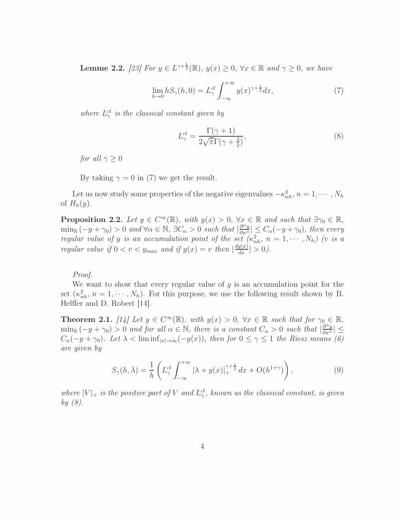
Lemme 2.2. [23] For y ∈ Lγ+ 12 (R), y(x) ≥ 0, ∀x ∈ R and γ ≥ 0, we have

limh→0

hSγ(h, 0) = Lclγ

∫ +∞

−∞

y(x)γ+12dx, (7)

where Lclγ is the classical constant given by

Lclγ =

Γ(γ + 1)

2√πΓ(γ + 3

2), (8)

for all γ ≥ 0

By taking γ = 0 in (7) we get the result.

Let us now study some properties of the negative eigenvalues −κ2nh, n = 1, · · · , Nh

of Hh(y).

Proposition 2.2. Let y ∈ C∞(R), with y(x) > 0, ∀x ∈ R and such that ∃γ0 ∈ R,minR (−y + γ0) > 0 and ∀α ∈ N, ∃Cα > 0 such that | ∂αy

∂xα | ≤ Cα(−y+ γ0), then everyregular value of y is an accumulation point of the set (κ2nh, n = 1, · · · , Nh) (v is a

regular value if 0 < v < ymax and if y(x) = v then |dy(x)dx

| > 0).

Proof.We want to show that every regular value of y is an accumulation point for the

set (κ2nh, n = 1, · · · , Nh). For this purpose, we use the following result shown by B.Helffer and D. Robert [14].

Theorem 2.1. [14] Let y ∈ C∞(R), with y(x) > 0, ∀x ∈ R such that for γ0 ∈ R,minR (−y + γ0) > 0 and for all α ∈ N, there is a constant Cα > 0 such that | ∂αy

∂xα | ≤Cα(−y + γ0). Let λ < lim inf |x|→∞(−y(x)), then for 0 ≤ γ ≤ 1 the Riesz means (6)are given by

Sγ(h, λ) =1

h

(

Lclγ

∫ +∞

−∞

|λ+ y(x)|γ+12

+ dx+O(h1+γ)

)

, (9)

where |V |+ is the positive part of V and Lclγ , known as the classical constant, is given

by (8).

4

We put γ = 0 in (6). We notice that S0(h, λ) = Nh(λ, y). Substituting γ by 0 in(9), we get

S0(h, λ) =1

hLcl0

∫ +∞

−∞

√

|λ+ y(x)|+dx+O(1). (10)

We suppose that there is a regular value y0 of y that is not an accumulation pointof the set (κ2nh, n = 1, · · · , Nh). So there is a neighborhood V (y0) of y0 and a valueh0, small enough such that ∀h < h0, V (y0) does not contain any element element κ2nh.

Moreover, we can choose V (y0) small enough such that

inf{|dy(x)dx

|, for x such that y(x) ∈ V (y0)} = c > 0. (11)

Then, we can take V (y0) = [y1, y2[, with y1 and y2 some regular values of y and0 < y1 < y2.

For all h < h0, the difference S0(h,−y1) − S0(h,−y2) represents the number ofelements of (−κ2nh, n = 1, · · · , Nh) in the interval ] − y2,−y1]. However this set isempty because there is no element in the neighborhood of y0.

Denoting X(λ) = {x|y(x) + λ ≥ 0}, we have from (10)

S0(h,−y1)−S0(h,−y2) =1

hLcl0

(∫

X(−y1)

√

y(x)− y1dx−∫

X(−y2)

√

y(x)− y2dx

)

+ O(1), (12)

so, as the left quantity is null, we obtain∫

X(−y1)

√

y(x)− y1dx =

∫

X(−y2)

√

y(x)− y2dx, (13)

and we have X(−y1) = X(−y2) ∪ y−1([y1, y2[), so∫

X(−y2)

√

y(x)− y1dx+

∫

y−1([y1,y2[)

√

y(x)− y1dx =

∫

X(−y2)

√

y(x)− y2dx, (14)

∫

X(−y2)

(√

y(x)− y1 −√

y(x)− y2)dx+

∫

y−1([y1,y2[)

√

y(x)− y1dx = 0. (15)

Hence as these two integrals are positives, we get∫

y−1([y1,y2[)

√

y(x)− y1dx = 0, (16)

5

therefore |y(x)− y1| = 0 almost everywhere in y−1([y1, y2[), then y1 = y2, which is acontradiction.

Now, proposition 2.2 introduces an interesting property of the SCSA. Indeed,remembering that

− h2d2ψnh(x)

dx2− y(x)ψnh(x) = −κ2nhψnh(x). (17)

and by multiplying the previous equation by ψnh(x) and integrating it by part weget

κ2nh =

∫ +∞

−∞

yψ2nh(x)dx− h2

∫ +∞

−∞

(

dψnh(x)

dx

)2

dx. (18)

Then, we notice that −ymax ≤ −κ2nh < 0 as it is illustrated in figure 1. Hence, fora fixed value of h, κ2nh can be interpreted as particular values of y which define anew quantization approach that can be interpreted by semi-classical concepts. TheSCSA appears then as a new way to quantify a signal.

1.6 1.8 2 2.2 2.4 2.6 2.8 3−45

−40

−35

−30

−25

−20

−15

−10

−5

0

x

−y(

x)

−κ1h2

−κ2h2

−κ3h2

−κ11h2

Figure 1: The negative spectrum of the Schrödinger operator −h2 d2

dx2−y(x) provides

a quantization of the signal y

To finish this section, we examine the convergence of the first two momentums ofκnh when h→ 0 through proposition 2.3. These quantities could be very interestingin signal analysis as it is mentioned in section 5 and also in a recent study [20].

6

Proposition 2.3. Under hypothesis (2), we have

limh→0

h

Nh∑

n=1

κnh =1

4

∫ +∞

−∞

y(x)dx, (19)

and remembering that

yh(x) = 4h

Nh∑

n=1

κnhψ2nh(x), x ∈ R, (20)

we have

limh→0

∫ +∞

−∞

yh(x)dx =

∫ +∞

−∞

y(x)dx. (21)

Moreover if y ∈ L2(R), then,

limh→0

h

Nh∑

n=1

κ3nh =3

16

∫ +∞

−∞

y2(x)dx. (22)

Proof. The limits (19) and (22) are deduced from lemma 2.2 for γ =1

2and γ =

3

2respectively,

limh→0

h

Nh∑

n=1

κnh =1

4

∫ +∞

−∞

y(x)dx, (23)

limh→0

h

Nh∑

n=1

κ3nh =3

16

∫ +∞

−∞

y2(x)dx. (24)

By integrating (3) we have

∫ +∞

−∞

yh(x)dx = 4h

Nh∑

n=1

κnh. (25)

Then, combining (25) and (19), we get (21).

7

3 Exact representation and reflectionless potentials

In this section, we are interested in an exact representation of a signal for a fixedh and its relation to reflectionless potentials (reflectionless potentials are definedin the appendix B) of the Schrödinger operator as it is described in the followingproposition:

Proposition 3.1. The following properties are equivalent,

i) Equality in (19) holds for a finite h ;

ii) ∃h such that yh = y ;

iii) ∃h such thaty

h2is a reflectionless potential of H1(V ).

ProofThe following proof uses some concepts and results from scattering transform

theory that are recalled in the appendix. First, we suppose that i) is fulfilled then

∃h,∫ +∞

−∞

y(x)dx = 4h

Nh∑

n=1

κnh. (26)

Writing the first invariant 56 (see the appendix C) for the potential − y

h2we have

∫ +∞

−∞

y(x)dx = 4h

Nh∑

n=1

κnh +h2

π

∫ +∞

−∞

ln (1− |Rr(l)h(k)|2)dk, (27)

where Rr(l)h(k) is the reflection coefficient (see the appendix A).Using (25), we get

∫ +∞

−∞

y(x)dx =

∫ +∞

−∞

yh(x)dx+h2

π

∫ +∞

−∞

ln (1− |Rr(l)h(k)|2)dk. (28)

Then, from (30) and (28) we obtain

∫ +∞

−∞

ln (1− |Rr(l)h(k)|2)dk = 0. (29)

The reflection coefficient of a Schrödinger operator satisfies |Rr(l)h(k)| ≤ 1, ∀k ∈ R

(see for exemple [6]). Then, we get ln (1− |Rr(l)h(k)|2) ≤ 0. Equality (29) is then

8

fulfilled if and only if ln (1− |Rr(l)h(k)|2) = 0, k ∈ R a.e; which is true only if|Rr(l)h(k)| = 0, k ∈ R a.e. This property defines a reflectionless potential. So,i) ⇒ iii).

Now, using the Deift-Trubowitz formula (52) (see appendix B) that we rewrite

for the potential − y

h2and taking Rr(l)h(k) = 0, we can deduce that statement (iii)

implies statement (ii).Then, if we suppose that yh = y for a given value of h we have

∫ +∞

−∞

yh(x)dx =

∫ +∞

−∞

y(x)dx, (30)

hence ii) ⇒ i)

4 Numerical results

In this section, we are interested in the validation of the SCSA through somenumerical examples. For this purpose, it will be more convenient to consider the

problem associated to H1(y

h2). Therefore, in order to simplify the notations, we put

1

h2= χ, Nh = Nχ and

κ2nhh2

= κ2nχ, n = 1, · · · , Nχ. We denote the L2-normalized

eigenfunctions ψnχ, n = 1, · · · , Nχ. Formula (3) is then rewritten

yχ(x) =4

χ

Nχ∑

n=1

κnχψ2nχ(x), x ∈ R, (31)

We start by giving the numerical scheme used to estimate a signal with theSCSA. Then, the sech-squared function will be considered. This example illustratesthe influence of the parameter χ on the approximation. Gaussian, sinusoidal andchirp signals will be also considered.

4.1 The numerical scheme

The first step in the SCSA is to solve the spectral problem of a one dimensionalSchrödinger operator. Its discretization leads to an eigenvalue problem of a matrix.In this work, we propose to use a Fourier pseudo-spectral method [15], [30]. Thelatter is well-adapted for periodic problems but in practice it gives good results forsome non-periodic problems for instance, rapid decreasing signals.

9

We consider a grid of M equidistant points xj , j = 1, · · · ,M such that

a = x1 < x2 < · · · < xM−1 < xM = b. (32)

Let ∆x =b− a

M − 1be the distance between two consecutive points. We denote yj and

ψj the values of y and ψ at the grid points xj , j = 1, · · · ,Myj = y(xj), ψj = ψ(xj), j = 1, · · · ,M. (33)

Therefore, the discretization of the Schrödinger eigenvalue problem leads to thefollowing eigenvalue matrix problem

(−D2 − χ diag (Y ))ψ = λψ, (34)

where diag(Y ) is a diagonal matrix whose elements are yj, j = 1, · · · ,M and ψ =

[ψ1 ψ2, · · · ψM−1 ψM ]T . D2 is the second order differentiation matrix given by [30],

• If M is even

D2(k, j) =∆2

(∆x)2

−π2

3∆2− 1

6for k = j,

− (−1)k−j 1

2

1

sin2(

(k−j)∆2

) for k 6= j.(35)

• If M is odd

D2(k, j) =∆2

(∆x)2

−π2

3∆2− 1

12pour k = j,

− (−1)k−j 1

2

1

sin(

(k−j)∆2

) cot(

(k−j)∆2

)

pour k 6= j,

(36)

with ∆ =2π

M. the matrix D2 is symmetric and definite negative. To solve the

eigenvalue problem of the matrix (−D2 − χ diag(Y )) we use the Matlab routine eig.The final step in the SCSA algorithm is to find an optimal value of the parameter

χ. So we look for a value χ̂ that gives a good approximation of y with a small numberof negative eigenvalues. From the numerical tests, we noticed that the number Nχ

is in general a step by step function of χ. So, we optimize the following criteria ineach interval [χ1, χ2] where Nχ is constant,

J(χ) =1

M

M∑

i=1

(yi − yχi)2, yχi =

4

χ

Nχ∑

n=1

κnχψ2niχ, i = 1, · · · ,M. (37)

10

Figure 2: The SCSA algorithm

For χ large enough (equivalently h small enough), we know an approximate relationbetween the number of negative eigenvalues and χ thanks to proposition 2.1. Then,we can deduce approximate values of χ1 and χ2 according to a given number ofnegative eigenvalues. Fig. 2 summarizes the SCSA algorithm.

Remark: In practice, we often omit the optimization step and just fix Nχ to alarge enough value.

4.2 The sech-squared function

In order to illustrate the influence of the parameter χ on the SCSA, we first studya sech-squared function given by

y(x) = sech2(x− x0), x ∈ R. (38)

11

The potential of the Schrödinger operatorH1(χy) is given in this case by: −χ sech2(x−x0). This potential is called in quantum physics Pöschl-Teller potential.

It is well-known that the Pöschl-Teller potential belongs to the class of reflec-tionless potentials if,

χ = χp = N(N + 1), N = 1, 2, 3, · · · , (39)

N being the number of negative eigenvalues of H1(χy) [22].So, for example, if χ = 2, the Schrödinger operator spectrum is negative and

consists of a single negative eigenvalue given by λ = −1. If χ = 6, there are twonegative eigenvalues: λ1 = −4, λ2 = −1 and so on.

Let us now apply the SCSA to reconstruct y. For this purpose, we must truncatethe signal and consider it on a finite interval so that the numerical computationscould be possible.

Figure 3.a illustrates the variation of the mean square error and Nχ according toχ. We notice that,

• Nχ is an increasing function of χ as described in proposition (2.1). Moreover,Nχ is a step by step function.

• There are some particular values of χ for which the error is minimal. Thesevalues are in fact the particular values χp = Nχ(Nχ + 1), Nχ = 1, 2, · · · forwhich −χy is a reflectionless potential.

• For all ǫ > 0, there is a value χ = χǫ such that ∀χ > χǫ, J(χ) < ǫ.

Figure 3.b illustrates the variation of the first four eigenvalues of the matrix−D2 −χ diag(Y ), settled in an increasing way, according to χ. We notice that theseeigenvalues, initially positive, are decreasing functions of χ and at every passage fromNχ to Nχ + 1, a positive eigenvalue becomes negative.

Otherwise, in figure 4, the first four squared eigenfunctions ψ2nχ, n = 1, · · · , 4 are

represented for χ = 20. Each ψ2nχ has n− 1 zeros.

Figure 5 shows a satisfactory reconstruction of y for Nχ = 1, 2, 3 and 4.

12

0 5 10 15 20 25 301

2

3

4

5

χ

Number of negative eigenvalues

0 5 10 15 20 25 300

1

2

3

4x 10

−3

χ

Mean square error

0 5 10 15 20 25 30−30

−25

−20

−15

−10

−5

0

5

χ

The

four

firs

t eig

enva

lues

(a) (b)

Figure 3: (a) Mean square error and number of negative eigenvalues according toχ for y(x) = sech2(x − 6) in [0, 15]. (b) Four first eigenvalues according to χ fory(x) = sech2(x− 6) in [0, 15]

0 5 10 150

0.2

0.4

0.6

0.8

1

1.2

1.4

x

ψ12 (x

)

0 5 10 150

0.1

0.2

0.3

0.4

0.5

0.6

0.7

x

ψ22 (x

)

0 5 10 150

0.1

0.2

0.3

0.4

0.5

0.6

0.7

x

ψ32 (x

)

0 5 10 150

0.05

0.1

0.15

0.2

0.25

0.3

0.35

x

ψ42 (x

)

Figure 4: Four first eigenfunctions ψ2nχ for χ = 20 for y(x) = sech2(x− 6) in [0, 15]

13

0 5 10 150

0.1

0.2

0.3

0.4

0.5

0.6

0.7

0.8

0.9

1

x

y(x)

Nχ=1

Real signal

Estimated signal

0 5 10 150

0.1

0.2

0.3

0.4

0.5

0.6

0.7

0.8

0.9

1

x

y(x)

Nχ=2

Real signal

Estimated signal

0 5 10 150

0.1

0.2

0.3

0.4

0.5

0.6

0.7

0.8

0.9

1

x

y(x)

Nχ=3

Real signal

Estimated signal

0 5 10 150

0.2

0.4

0.6

0.8

1

1.2

1.4

x

y(x)

Nχ=4

Real signal

Estimated signal

Figure 5: Estimation of y(x) = sech2(x − 6) in [0, 15], from the left to the right:Nχ = 1, Nχ = 2 (top). Nχ = 3, Nχ = 4 (bottom)

14

4.3 Estimation of some signals

In this section, we are interested in the estimation of some signals with the SCSA.In each case, we represent the estimation error, the number of negative eigenvaluesaccording to χ and the real and estimated signals for different values of χ.

We start with a gaussian signal given by:

y(x) =1

σ√2πe−

(x−µ)2

2σ2 . (40)

For the numerical tests we take σ = 0.1 and µ = 0.75.Figures 6 and 7 illustrate the results. We notice that with Nχ = 2, the estimation

is satisfactory and as Nχ increases better is the approximation.

0 50 100 150 200 250 300 350 4001

2

3

4

5

χ

Number of negative eigenvalues

0 50 100 150 200 250 300 350 4000

0.05

0.1

0.15

0.2

χ

Mean square error

Figure 6: Mean square error and number of negative eigenvalues according to χ fora gaussian signal

Now we are interested in a sinusoidal signal defined in a finite interval I,

y(x) =

{

A sin(ωx+ φ) x ∈ I

0 otherwise(41)

This signal has negative values, so to apply the SCSA, we must translate the signalby ymin = −A such that y − ymin > 0. The Schrödinger operator potential to beconsidered is then given by −χ(y − ymin). For the numerical tests, we took A = 2,ω = π and φ = −0.5.

15

0 0.2 0.4 0.6 0.8 1 1.2 1.4 1.6 1.8 20

0.5

1

1.5

2

2.5

3

3.5

4

4.5

x

y(x)

Nχ=1

Real signal

Estimated signal

0 0.2 0.4 0.6 0.8 1 1.2 1.4 1.6 1.8 20

0.5

1

1.5

2

2.5

3

3.5

4

x

y(x)

Nχ=2

Real signal

Estimated signal

0 0.2 0.4 0.6 0.8 1 1.2 1.4 1.6 1.8 20

0.5

1

1.5

2

2.5

3

3.5

4

4.5

x

y(x)

Nχ=3

Real signal

Estimated signal

0 0.2 0.4 0.6 0.8 1 1.2 1.4 1.6 1.8 20

0.5

1

1.5

2

2.5

3

3.5

4

x

y(x)

Nχ=4

Real signal

Estimated signal

Figure 7: Estimation of a gaussian signal, from the left to the right: Nχ = 1, Nχ = 2(top). Nχ = 3, Nχ = 4 (bottom)

16

The results are represented in figures 8, 9 and 10. In 9, a single period of thesignal is considered while in 10, four periods are represented. In the last case wenoticed that the negative eigenvalues are of multiplicity 4, they are repeated in eachperiod.

0 50 100 150 200 250 300 350 4000

5

10

15

20

χ

Number of negative eigenvalues

0 50 100 150 200 250 300 350 4000

0.02

0.04

0.06

χ

Mean square error

Figure 8: Mean square error and number of negative eigenvalues according to χ fora sinusoidal signal

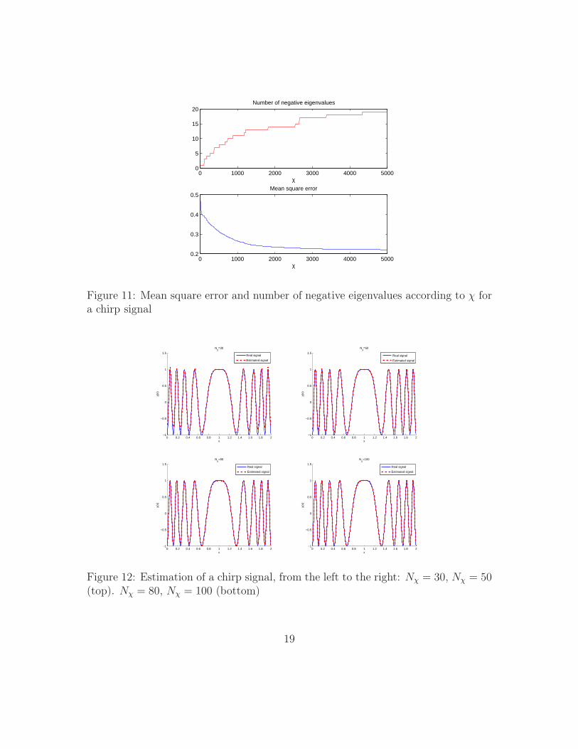
Finally, figures 11 and 12 illustrate the results obtained in the case of a chirpsignal. We recall that a chirp signal is usually defined by a time varying frequencysinusoid. In our tests, we considered a linear variation of the frequency.

5 Arterial blood pressure analysis with the SCSA

ABP plays an important role in the cardiovascular system. So many studies weredone aiming at proposing mathematical models in order to understand the cardio-vascular system both in healthy and pathological cases. Despite the large numberof ABP models, the interpretation of ABP in clinical practice is often restricted tothe interpretation of the maximal and the minimal values called respectively thesystolic pressure and the diastolic pressure. None information on the instantaneousvariability of the pressure is given in this case. However, pertinent information canbe extracted from ABP waveform. The SCSA seems to provide a new tool for theanalysis of ABP waveform. This section presents some obtained results.

17

0 0.2 0.4 0.6 0.8 1 1.2 1.4 1.6 1.8 2−2

−1.5

−1

−0.5

0

0.5

1

1.5

2

x

y(x)

Nχ=4

Real signal

Estimated signal

0 0.2 0.4 0.6 0.8 1 1.2 1.4 1.6 1.8 2−2

−1.5

−1

−0.5

0

0.5

1

1.5

2

x

y(x)

Nχ=6

Real signal

Estimated signal

0 0.2 0.4 0.6 0.8 1 1.2 1.4 1.6 1.8 2−2

−1.5

−1

−0.5

0

0.5

1

1.5

2

x

y(x)

Nχ=8

Real signal

Estimated signal

0 0.2 0.4 0.6 0.8 1 1.2 1.4 1.6 1.8 2−2

−1.5

−1

−0.5

0

0.5

1

1.5

2

x

y(x)

Nχ=10

Real signal

Estimated signal

Figure 9: Estimation of a sinusoidal signal, from the left to the right: Nχ = 4, Nχ = 6(top). Nχ = 8, Nχ = 10 (bottom)

0 1 2 3 4 5 6 7 8−2

−1.5

−1

−0.5

0

0.5

1

1.5

2

x

y(x)

Real signal

Estimated signal

Figure 10: Estimation of 4 sinusoidal signal periods with Nχ = 10

18

0 1000 2000 3000 4000 50000

5

10

15

20

χ

Number of negative eigenvalues

0 1000 2000 3000 4000 50000.2

0.3

0.4

0.5

χ

Mean square error

Figure 11: Mean square error and number of negative eigenvalues according to χ fora chirp signal

0 0.2 0.4 0.6 0.8 1 1.2 1.4 1.6 1.8 2−1

−0.5

0

0.5

1

1.5

x

y(x)

Nχ=30

Real signal

Estimated signal

0 0.2 0.4 0.6 0.8 1 1.2 1.4 1.6 1.8 2−1

−0.5

0

0.5

1

1.5

x

y(x)

Nχ=50

Real signal

Estimated signal

0 0.2 0.4 0.6 0.8 1 1.2 1.4 1.6 1.8 2−1

−0.5

0

0.5

1

1.5

x

y(x)

Nχ=80

Real signal

Estimated signal

0 0.2 0.4 0.6 0.8 1 1.2 1.4 1.6 1.8 2−1

−0.5

0

0.5

1

1.5

x

y(x)

Nχ=100

Real signal

Estimated signal

Figure 12: Estimation of a chirp signal, from the left to the right: Nχ = 30, Nχ = 50(top). Nχ = 80, Nχ = 100 (bottom)

19

We denote the ABP signal P and P̂ its estimation using the SCSA such that

P̂ (t) =4

χ

Nχ∑

n=1

κnχψ2nχ(t), (42)

where −κ2nχ, n = 1, · · · , Nχ are the Nχ negative eigenvalues of H1(χP ) and ψnχ theassociated L2−normalized eigenfunctions. As ABP signal is a function of time, weuse the time variable t in the Schrödinger equation instead of the space variable x.

The ABP signal was estimated for several values of the parameter χ and henceNχ. Figure 13 illustrates the measured and estimated pressures for one beat of ABPand the estimated error with Nχ = 9. Signals measured at the aorta level and thefinger respectively were considered. We point out that 5 to 9 negative eigenvaluesare sufficient for a good estimation of ABP signals [17], [19].

A first interest in using the SCSA for ABP analysis is to decompose the signalinto its systolic and diastolic parts respectively. This application was inspired froma reduced model of ABP based on solitons introduced in [4], [18]. Solitons are in factsolutions of some nonlinear partial derivative equations for instance the Korteweg-deVries (KdV) equation which was considered in this reduced model [4]. This modelproposes to write the ABP as the sum of two terms: and N-soliton, solution of theKdV equation describing fast phenomena that predominate during the systolic phaseand a two-elements windkessel model that describes slow phenomena during thediastolic phase. Moreover the KdV equation can be solved with the Inverse ScatteringTransform (IST) whose definition is recalled in appendix A. In this approach, theKdV equation is associated to a one dimensional Schrödinger potential parameterizedby time where the potential is given by the solution of the KdV equation at a giventime. Therefore a relation between the Schrödinger operator and solitons was found[10]: solitons are reflectionless potentials. Then according to proposition 3.1, theSCSA coincides with a soliton representation of a signal for a finite χ when −χy isan Nχ-soliton, where Nχ denotes the number of negative eigenvalues 1 of H1(χy).So each spectral component represents a single soliton. We know that solitons arecharacterized by their velocity which is determined by the negative eigenvalues −κ2nχ,n = 1, · · · , Nχ of the Schrödinger operator. The largest values κnχ characterize fastcomponents and the small values of κnχ characterize slow components. From theseremarks, we propose to decompose equation (31) into two partial sums: the first one,composed of the Ns (Ns = 1, 2, 3 in general) largest κnχ and the second partial sumcomposed of the remaining components. The first partial sum describes the systolic

1Each soliton is characterized by a negative eigenvalue

20

1.6 1.8 2 2.2 2.4 2.6 2.8 350

55

60

65

70

75

80

85

90

95

t (s)

Art

eria

l blo

od p

ress

ure

(mm

Hg)

Estimated pressureMeasured pressure

1.6 1.8 2 2.2 2.4 2.6 2.8 30

0.5

1

1.5

2

2.5

t (s)

Rel

ativ

e er

ror

(%)

(a) Aorta

1.6 1.8 2 2.2 2.4 2.6 2.8 350

60

70

80

90

100

110

120

130

140

t (s)

Are

tria

l blo

od p

ress

ure

(m

mH

g)

Estimated pressureMeasured pressure

1.6 1.8 2 2.2 2.4 2.6 2.8 30

0.5

1

1.5

2

2.5

3

t (s)

Rel

ativ

e er

ror

(%)

(b) Finger

Figure 13: Reconstruction of the pressure at the aorta and the finger level with theSCSA and Nχ = 9. On the left the estimated and measured pressures, On the rightthe relative error

21

phase and the second one describes the diastolic phase. We denote P̂s and P̂d thesystolic pressure and the diastolic pressure respectively estimated with the SCSA.Then we have

P̂s(t) =4

χ

Ns∑

n=1

κnχψ2nχ(t), P̂d(t) =

4

χ

Nχ∑

n=Ns+1

κnχψ2nχ(t). (43)

Figure 14 represents the measured pressure and the estimated systolic and di-astolic pressures respectively. We notice that P̂s and P̂d are respectively localizedduring the systole and the diastole.

1.6 1.8 2 2.2 2.4 2.6 2.8 30

10

20

30

40

50

60

70

80

90

100

t (s)

Art

eria

l blo

od p

ress

ure

(mm

Hg)

Estimated systolic pressure

Measured pressure

1.6 1.8 2 2.2 2.4 2.6 2.8 320

30

40

50

60

70

80

90

100

t (s)

Art

eria

l blo

od p

ress

ure

(m

mH

g)

Estimated diastolic pressureMeasured pressure

Figure 14: On the left the estimated systolic pressure. On the right estimateddiastolic pressure

6 Discussion

The spectral analysis of the Schrödinger operator introduces two inverse prob-lems: an inverse spectral problem and an inverse scattering problem.

On the one hand, the inverse spectral problem aims at reconstructing the po-tential of a Schrödinger operator with its spectrum (spectral function). It has beenextensively studied for instance by Borg, Gel’Fand, Levitan and Marchenko [11] ormore recently by Ramm [27]. They considered the half-line case and used two spectraof the Schrödinger operator with two different boundary conditions in order to recon-struct the potential. The inverse spectral problem for a semi-classical Schrödingeroperator Hh(y) have been recently considered for example by Colin de Verdiére [5]

22

who proposed to reconstruct the potential locally with a single spectrum or Guilleminand Uribe [13] who showed that under some assumptions, the low-lying eigenvaluesof the operator determine the Taylor series of the potential at the minimum.

In this work we have studied an inverse spectral approach that is different fromclassical inverse spectral problems. Indeed, we used more information to reconstructthe potential by including the eigenfunctions as illustrated by equation (3).

On the other hand, the inverse scattering problem aims at recovering the potentialfrom the scattering data (see appendix A). Many studies considered this questionfor instance those of Marchenko [25] who proved that under some conditions onthe scattering data, a potential in L1

1(R) can be reconstructed from these scatteringdata and gave an algorithm for recovering the potential. We can also quote worksof Faddeev [9], Deift and Trubowitz [6] considering potentials in L1

1(R), Dubrovin,Matveev and Novikov [7] for periodic potentials.

The convergence of the SCSA when h→ 0 is not easy to study. Using the Deift-Trubowitz formula (52) we have tried to consider this problem. However, despiteinteresting results obtained regarding the convergence of some quantities dependingonly on the continuous spectrum of the Schrödinger operator to zero, we did notsucceed in finding a result of convergence for yh. A study supported by semi-classicalconcepts is now under consideration. The latter is based on the generalization of theresults of G. Karadzhov [16].

The SCSA method has given promising results in the analysis of arterial bloodpressure waveforms. More than a good reconstruction of these signals, the SCSAintroduces interesting parameters that give relevant physiological information. Theseparameters are the negative eigenvalues and the invariants which are given by themomentums of κnχ, n = 1, · · · , Nχ introduced in proposition 2.3. For example,these new cardiovascular indices allow the discrimination between healthy patientsand heart failure subjects [21]. A recent study [20] shows that the first systolicmomentum (associated to the systolic phase) gives information on stroke volumevariation, a physiological parameter of great interest.

We have seen in proposition 3.1 that for a fixed value of h the SCSA coincideswith a reflectionless potentials approximation. This point seems to be an interestingavenue of research. Indeed, thanks to the relation between reflectionless potentialsand solitons, the approximation by reflectionless potentials could have interestingapplications in signal analysis and in particular in data compression. As we said inthe previous section, solitons are reflectionless potentials of the Schrödinger opera-tor. Gardner et al [10] showed that an N -soliton is completely determined by thediscrete scattering data and in particular by 2N parameters which are the negativeeigenvalues and the normalizing constants. Hence, if −χy is an Nχ-soliton, it is given

23

by the following formula:

y(x) =2

χ

∂2

∂x2ln (det (I + Aχ))(x), x ∈ R, (44)

Aχ(x) is an Nχ×Nχ matrix of coefficients

Aχ(x) =

[

cmχcnχ

κmχ+κnχe−(κmχ+κnχ)x

]

n,m

, n,m = 1, · · · , Nχ, (45)

where −κ2nχ and cnχ, n = 1, · · · , Nχ are the negative eigenvalues and the normaliz-ing constants of H1(χy). Hence, this formula provides a parsimonious representationof a signal.

The convergence of the approximation by solitons (or reflectionless potentials)when χ → +∞ (equivalently h → 0) was studied by Lax and Levermore [24] in adifferent context. Indeed they studied the small dispersion limit of the KdV equationand approached the initial condition of the KdV equation by an N -soliton thatdepends on the small dispersion parameter which is in our case h. They showedthe results in the mono-well potential case and affirmed without prove that theresult remain still true for multi-well potentials. However the main limitation of thisapproach is the difficulty to compute the normalizing constants. This difficulty canbe explained by the fact that these constants are defined at infinity which can notbe handled in the numerical implementation. At the best of our knowledge there isno study enabling the computation of these parameters apart a recent attempt bySorine et al [29].

7 Conclusion

A new method for signal analysis based on a semi-classical approach has beenproposed in this study: the signal is considered as a potential of a Schrödingeroperator and then represented using the discrete spectrum of this operator. Somespectral parameters are then computed leading to a new approach for signal analysis.This study is a first step in the validation of the SCSA. Indeed, we have assessed herethe ability of the SCSA to reconstruct some signals. We have studied particularly achallenging application which is the analysis of the arterial blood pressure waveforms.The SCSA introduces a novel approach for arterial blood pressure waveform analysisand enables the estimation of relevant physiological parameters. A theoretical studyis now under consideration regarding the convergence of the SCSA for h → 0. Thework must be orientated at a second step to the comparison between the performance

24

of the SCSA and other signal analysis methods like Fourier transform or the waveletsand also to the generalization of the SCSA to other fields.

Acknowledgments

The authors thank Doctor Yves Papelier from the Hospital Béclère in Clamartfor providing us arterial blood pressure data.

A Direct and inverse scattering transforms

These appendices recall some known concepts on direct and inverse scatteringtransforms of a one-dimensional Schrödinger operator. For more details, the readercan refer to the large number of references on this subject for instance [1], [3], [6],[8], [9].

We consider here the spectral problem of a Schrödinger operator H1(−V ), givenby

− d2ψ

dx2+ V (x, t)ψ = k2ψ, k ∈ C

+, x ∈ R, (46)

where the potential V such that V ∈ B. For simplicity, we will omit the indice 1 ofthe spectral parameters in the following.

For k2 > 0, we introduce the solutions ψ± of equation (46) such that

ψ−(k, x) =

{

T (k)e−ikx x→ −∞,

e−ikx +Rr(k)e+ikx x→ +∞,

(47)

ψ+(k, x) =

{

T (k)e+ikx x→ +∞,

e+ikx +Rl(k)e−ikx x→ −∞,

(48)

where T (k) is called the transmission coefficient and Rl(r)(k) are the reflection coeffi-cients from the left and the right respectively. The solution ψ− for example describesthe scattering phenomenon for a wave e−ikx of amplitude 1, sent from +∞. Thiswave hit an obstacle which is the potential so that a part of the wave is transmittedT (k)e−ikx and the other part is reflected Rr(k)e

+ikx. ψ+ describes the scatteringphenomenon for a wave e+ikx sent from −∞.

For k2 < 0, the Schrödinger operator spectrum has N negative eigenvalues de-noted −κ2n, n = 1, · · · , N . The associated L2-normalized eigenfunctions are such

25

that

ψn(x) = clne−κnx, x → +∞, (49)

ψn(x) = (−1)N−ncrne+κnx, x→ −∞, (50)

cln and crn are the normalizing constants from the left and the right respectively.The spectral analysis of the Schrödinger operator introduces two transforms:

• The direct scattering transform (DST) which consists in determining the socalled scattering data for a given potential. Let us denote Sl(V ) and Sr(V ) thescattering data from the left and the right respectively:

Sj(V ) := {Rj(k), κn, cjn, n = 1, · · · , N}, j = l, r, (51)

where j = r if j = l and j = l if j = r.

• The inverse scattering transform (IST) that aims at reconstructing a potentialV using the scattering data.

The scattering transforms have been proposed to solve some partial derivativeequations for instance the KdV equation [10].

B Reflectionless potentials

Deift and Trubowitz [6] showed that when the Schrödinger operator potential Vsatisfies hypothesis (2) then it can be reconstructed using an explicit formula givenby

V (x) = −4N∑

n=1

κnψ2n(x) +

2i

π

∫ +∞

−∞

kRr(l)(k) f2±(k, x)dk, x ∈ R. (52)

This formula is called the Deift-Trubowitz trace formula. It is given by the sum oftwo terms: a sum of κnψ

2n that characterizes the discrete spectrum, and an integral

term that characterizes the contribution of the continuous spectrum.There is a special classe of potentials called reflectionless potentials for which the

problem is simplified. A reflectionless potential is defined by Rl(r)(k) = 0, ∀k ∈ R.According to the Deift-Trubowitz formula, a reflectionless potential can be writtenusing the discrete spectrum only,

V (x, t) = −4N∑

n=1

κnψ2n(x, t), (53)

26

C An infinite number of invariants

There is an infinite number of time invariants for the KdV equation given bythe conserved quantities [10], [12], [26]. Let us denote these invariants Im(V ), m =0, 1, 2, · · · . They are of the form

Im(V ) = (−1)m+12m+ 1

22m+2

∫ +∞

−∞

Pm(V,∂V

∂x,∂2V

∂x2, · · · )dx, (54)

where Pm, m = 0, 1, 2, · · · are known polynomials in V and its successive derivativeswith respect to x ∈ R [3].

A general formula relates Im(V ) to the scattering data of H1(−V ) [3], [12], [26]as follows:

Im(V ) =N∑

n=1

κ2m+1n +

2m+ 1

2π

∫ +∞

−∞

(−k2)m ln (1− |Rr(l)(k)|2)dk, (55)

m = 0, 1, 2, · · · . So, for m = 0, P0(V, · · · ) = V , we get with (54) and (55):

∫ +∞

−∞

V (x)dx = −4N∑

n=1

κn −1

π

∫ +∞

−∞

ln (1− |Rr(l)(k)|2)dk. (56)

References

[1] T. Aktosun and M. Klaus, Inverse theory: problem on the line, AcademicPress, London, 2001, ch. 2.2.4, pp. 770–785.

[2] Ph. Blanchard and J. Stubbe, Bound states for Schrödinger Hamiltonians:phase space methods and applications, Rev. Math. Phys., 35 (1996), pp. 504–547.

[3] F. Calogero and A. Degasperis, Spectral Transform and Solitons, NorthHolland, 1982.

[4] E. Crépeau and M. Sorine, A reduced model of pulsatile flow in an arterialcompartment, Chaos Solitons & Fractals, 34 (2007), pp. 594–605.

[5] Y. Colin de Verdière, A semi-classical inverse problem ii: Reconstructionof the potential, Preprint, (2008).

[6] P. A. Deift and E. Trubowitz, Inverse scattering on the line, Communica-tions on Pure and Applied Mathematics, XXXII (1979), pp. 121–251.

27

[7] B. A Dubrovin, V. B. Matveev, and S. P. Novikov, Nonlinear equationsof Korteweg-de Vries type, finite-zone linear operators, and Abelian varieties,Russian Math. Surveys, 31 (1976), pp. 59–146.

[8] W. Eckhaus and A. Vanharten, The Inverse Scattering Transformationand the Theory of Solitons, North-Holland, 1983.

[9] L. D. Faddeev, Properties of the S-matrix of the one-dimensional Schrödingerequation, Trudy Mat. Inst. Steklov, 73 (1964), pp. 314–336.

[10] C. S. Gardner, J. M. Greene, M. D. Kruskal, and R. M. Miura,Korteweg-de Vries equation and generalizations VI. Methods for exact solution,in Communications on Pure and Applied Mathematics, vol. XXVII, J.Wiley &Sons, 1974, pp. 97–133.

[11] I. M. Gel’fand and B. M. Levitan, On the determination of a differentialequation from its spectral function, Amer. Math. Soc. Transl., 2 (1955), pp. 253–304.

[12] F. Gesztesy and H. Holden, Trace formulas and conservation laws for non-linear evolution equations, Reviews in Mathematical Physics, 6 (1994), pp. 51–95.

[13] V. Guillemin and A. Uribe, Some inverse spectral results for semi-classicalschrödinger operators, Preprint, (2005).

[14] B. Helffer and D. Robert, Riesz means of bound states and semiclassi-cal limit connected with a Lieb-Thirring’s conjecture I, Asymptotic Analysis, 3(1990), pp. 91–103.

[15] M.Y. Hussaini, D. Gottlieb, and S. A. Orszag, Theory and applications ofspectral methods, in Spectral Methods for Partial Differential Equations, D. Got-tlieb R. Voigt and M. Hussaini, eds., 1984, pp. 1–54.

[16] G. Karadzhov, Asymptotique semi-classique uniforme de la fonction spectraled’opérateurs de Schrödinger. C.R. Acad. Sci. Paris, t. 310, Série I, p. 99-104(1990).

[17] T. M. Laleg, E. Crépeau, Y. Papelier, and M. Sorine, Arterial bloodpressure analysis based on scattering transform I, in Proc. EMBC, Sciences andTechnologies for Health, Lyon, France, August 2007.

28

[18] T. M. Laleg, E. Crépeau, and M. Sorine, Separation of arterial pressureinto a nonlinear superposition of solitary waves and a windkessel flow, Biomed-ical Signal Processing and Control Journal, 2 (2007), pp. 163–170.

[19] , Travelling-wave analysis and identification. A scattering theory framework,in Proc. European Control Conference ECC, Kos, Greece, July 2007.

[20] T. M. Laleg, C. Médigue, Y. Papelier, F. Cottin, and A. Van

de Louw, Validation of a new method for stroke volume variation assessment:a comparison with the picco technique, to appear in Annals of biomedical engi-neering.

[21] T. M. Laleg, C. Médigue, F. Cottin, and M. Sorine, Arterial bloodpressure analysis based on scattering transform II, in Proc. EMBC, Lyon, France,August 2007.

[22] L. D. Landau and E. M. Lifshitz, Quantum Mechanics: Non-RelativisticTheory, vol. 3, Pergamon Press, 1958.

[23] A. Laptev and T. Weidl, Sharp Lieb-Thirring inequalities in high dimen-sions, Acta Mathematica, 184 (2000), pp. 87–111.

[24] P. D. Lax and C. D. Levermore, The small dispersion limit of the Korteweg-de Vries equation I, II, III, Comm. Pure. & Appl. Math., 36 (1983), pp. 253–290,571–593, 809–828.

[25] V. A. Marchenko, Sturm-Liouville operators and applications, Birkhäuser,Basel, 1986.

[26] S. Molchanov, M. Novitskii, and B. Vainberg, First KdV integrals andabsolutely continuous spectrum for 1-d Schrödinger operator, Commun. Math.Phys, 216 (2001), pp. 195–213.

[27] A. G. Ramm, A new approach to the inverse scattering and spectral problemsfor the strum-liouville equation, Annal. der Physik, 7 (1998), pp. 321–338.

[28] M. Reed and B. Simon, Methods of modern mathematical physics, IV. Anal-ysis of operators theory, Academic Press, New York, 1978.

[29] M. Sorine, Q. Zhang, T. M. Laleg, and E. Crepeau, Parsimoniousrepresentation of signals based on scattering transform, in IFAC’08, July 2008.

[30] L. N. Trefethen, Spectral Methods in Matlab, SIAM, 2000.

29