ARTICLE IN PRESS

0278-4343/$ - se

doi:10.1016/j.cs

�Correspondi

902-494-2885.

E-mail addre

(R.J. Greatbatc

Continental Shelf Research 24 (2004) 2149–2165

www.elsevier.com/locate/csr

The semi-prognostic method

Richard J. Greatbatcha,�, Jinyu Shenga, Carsten Edenb, Liqun Tanga,Xiaoming Zhaia, Jun Zhaoa

aDepartment of Oceanography, Dalhousie University, Halifax, Nova Scotia, Canada B3H 4J1bIFM-GEOMAR Kiel, Dusternbrooker Weg 20, D-24105 Kiel, Germany

Available online 4 October 2004

Abstract

An overview is given of the semi-prognostic method, a new and novel technique that can be used for adjusting models

to correct for systematic error. Applications of the method to a regional model of the northwest Atlantic Ocean, and to

an eddy-permitting model of the entire North Atlantic, show improvement in the handling of the Gulf Stream/North

Atlantic Current systems, especially in the ‘‘northwest corner’’ region southeast of Newfoundland where prognostic

models show systematic errors of as much as 10 1C in the temperature field. Use of the semi-prognostic method also

leads to improvement in the modelled flow over the eastern Canadian shelf. An advantage of the semi-prognostic

method is that it is adiabatic; in particular, in spite of the improvement seen in the modelled hydrography, the potential

temperature and salinity equations carried by the model are unchanged by the method. Rather, the method introduces a

correction term to the horizontal momentum equations carried by the model. Adiabaticity ensures that the method does

not compromise the requirement for the flow in the ocean interior to be primarily in the neutral tangent plane, and also

ensures that the method is well-suited for tracer studies. The method is also easy to implement, requiring only an

adjustment in the hydrostatic equation carried by the model. We also describe the use of the method as a diagnostic

tool, for probing the important dynamic processes governing a phenomenon, and finally as a technique for transferring

information between the different subcomponents of a nested modelling system.

r 2004 Elsevier Ltd. All rights reserved.

Keywords: Continental shelf; Modelling; Ocean basin; Ocean circulation; Atlantic Ocean; Scotian Shelf

1. Introduction

Models are often prone to systematic error.Examples are the tendency for the Gulf Stream to

e front matter r 2004 Elsevier Ltd. All rights reserve

r.2004.07.009

ng author. Tel.: +1-902-494-6674; fax: +1-

ss: richard.greatbatch@dal.ca

h).

separate too far to the north, and for a poorrepresentation of the region to the southeast ofNewfoundland known as the ‘‘northwest corner’’(Lazier, 1994), where the North Atlantic Currentturns first northward and then abruptly eastwardtowards Europe (see e.g. Willebrand et al., 2001).Associated with the poor representation of theGulf Stream system, the model sea surface

d.

ARTICLE IN PRESS

R.J. Greatbatch et al. / Continental Shelf Research 24 (2004) 2149–21652150

temperature (SST) can differ by as much as 10 1Cover large areas of the northwest Atlantic Ocean.Such large errors in SST can be expected to impactnegatively on both the North Atlantic storm trackin a coupled atmosphere/ocean modelling system(Hoskins and Valdes, 1990), and on the uptake oftracers such as carbon, both issues of importancefor climate modelling. In addition, poor represen-tation of ocean current systems in models can leadto erroneous pathways for tracers in models, andimpact negatively on the overall tracer budget (seeZhao et al., 2004, for an example).

In this paper, we describe a new and noveltechnique that can be used to correct models forsystematic error. The method, called ‘‘the semi-prognostic method’’, is a technique for transferringdata into a model or between models and wasoriginally introduced by Sheng et al. (2001). Shenget al. used a regional model for the northwesternpart of the North Atlantic Ocean, including theeastern Canadian shelf, to show that application ofthe semi-prognostic method leads to a significantimprovement in the representation of the GulfStream and the North Atlantic Current, includingthe circulation along the shelf break. Subse-quently, Eden et al. (2004) showed the success ofmodified versions of the method for improving theperformance of a 1=3� � 1=3� eddy-permittingmodel of the whole North Atlantic Ocean. Thebiggest improvements are again in the pathways ofthe Gulf Stream and the North Atlantic Currentsystem, but with the added bonus that the pole-ward heat transport by the model is brought intobetter accord with observational estimates. Themodifications introduced by Eden et al. (2004)avoid spurious damping of mesoscale eddy varia-bility and distortion of the model physics that are abyproduct of the method as it appeared in Shenget al. (2001). Eden and Greatbatch (2003) used themethod in a different context, this time exploitingthe distortion of the model physics to determinethe essential dynamics governing the behaviour ofa damped, decadal oscillation in a model of theNorth Atlantic. However, the method has applica-tion beyond it’s use as an adjustment or diagnostictechnique. In particular, it can be used in a nestedmodelling system as a means of transferringinformation between the different submodels (Zhai

et al., 2004). This is a new and exciting applicationof the method that is discussed in Section 4.

The principal advantages of the semi-prognosticmethod are (i) its simplicity and (ii) the fact it isadiabatic. The latter property arises because theadjustments to the model are made in thehorizontal momentum equations, leaving themodel tracer equations (in particular, the con-servation equations for potential temperature andsalinity) unchanged. As such, the method is idealfor tracer studies (see Zhao et al., 2004) since, likethe conservation equations for an active tracer, theconservation equations for a passive tracer areunchanged by the method. The semi-prognosticmethod can be contrasted with the robust diag-nostic method of Sarmiento and Bryan (1982). Inthe latter, the model tracer equations are adjustedby the addition of Newtonian relaxation terms.These relaxation terms hold the model tempera-ture and salinity close to climatology, but are alsoassociated with strong sources and sinks in themodel potential temperature and salinity equa-tions, with the result that the method is highlydiabatic. The advantages of using an adiabaticadjustment technique are discussed in Section 2.3.In Section 2.2, we note that the robust diagnosticmethod is an example of ‘‘nudging’’ (the diabaticrelaxation terms ‘‘nudge’’ the model potentialtemperature and salinity towards climatology). Inthe semi-prognostic method, on the other hand,the correction applied to the horizontal momen-tum equations does not have the form of arelaxation term. It follows that while the correc-tion term does ‘‘nudge’’, the direction of thenudging is not specified.

In this overview, we begin in Section 2.1 bydescribing the method as it appeared in Sheng etal. (2001). The interpretation of the method isdiscussed in Section 2.2, the advantages of anadiabatic approach in Section 2.3, and the distor-tion of the model physics and the use of themethod as a diagnostic technique (Eden andGreatbatch, 2003) in Section 2.4. This naturallyleads to a discussion of modified versions of themethod in Section 2.5, following Eden et al.(2004). Some applications of the semi-prognosticmethod are shown in Section 3, illustrating theimprovements in model performance. In Section 4,

ARTICLE IN PRESS

R.J. Greatbatch et al. / Continental Shelf Research 24 (2004) 2149–2165 2151

we briefly describe the use of the semi-prognosticmethod as a technique for nesting models, andfinally, in Section 5, we provide a summary andconclusions.

2. Formulation and interpretation

2.1. The standard method

The semi-prognostic method is applicable tohydrostatic models. For simplicity, we begin byconsidering models that use height coordinates inthe vertical, that is the common z-coordinate,where z measures geopotential height from areference level, or sigma-coordinate in which themodel vertical coordinate varies between 0 at thesea surface to �1 at the ocean bottom (seeGreatbatch and Mellor (1999) for a review of thedifferent vertical coordinates used in models).Application to models using other vertical coordi-nate systems are discussed briefly in Section 2.7.As applied to height coordinate models, the semi-prognostic method involves replacing the instan-taneous density variable in the model hydrostaticequation by a linear combination of the modeldensity, rm; and the input density rc: Usually thelatter is computed from climatological hydro-graphic data,1 but it might also be density fromthe same model (as when the method is being usedas a diagnostic tool; Eden and Greatbatch, 2003)or a different model (as in a nested modellingsystem, e.g. Zhai et al. (2004)). For simplicity, inthis and the next section, we assume that rc is theclimatological density unless stated otherwise. Itfollows that the model hydrostatic equation ischanged from

@p

@z¼ �grm (1)

to

@p

@z¼ �g½arm þ ð1� aÞrc; (2)

1In the applications to be described, we have used gridded

data. Use of the ‘‘smoothed’’ and ‘‘tapered’’ methods described

in Section 2.5 helps to reduce the effects of mismatches between

the input data and the bottom topography.

where p is the pressure variable carried by themodel and a is a parameter with 0pap1: If r ¼

rðy;S; pref Þ is the model equation of state (here y ispotential temperature, S is salinity), then

rm ¼ rðym;Sm; pref Þ (3)

and

rc ¼ rðyc;Sc; pref Þ; (4)

where ym;Sm are the instantaneous, prognosticpotential temperature and salinity variables car-ried by the model and yc;Sc are the inputclimatological potential temperature and salinitydata. It should be noted that (2) is applied at eachtime step, so that ym;Sm are evolving with time,and yc;Sc are usually seasonally varying. Here, wehave assumed a simplified equation of state inwhich the pressure dependence is replaced by anapproximation, pref ; to the actual pressure, withpref depending only on height, z (Dewar et al.,1998). However, there is no restriction thatprevents using the full equation of state in whichpref is replaced by the physical pressure, p: (Asnoted below, p is not the same as the pressurevariable, p, carried by the model.)

We next note that if a ¼ 1; the model is a pureprognostic model, and there is no influence fromthe input density, rc: On the other hand, puttinga ¼ 0 turns the model into a diagnostic model (seeGreatbatch and Mellor (1999) for a discussion of‘‘diagnostic’’ versus ‘‘prognostic’’ models). Indiagnostic models, the model density, rm; playsno role in the model dynamics; in fact, in this limit,the potential temperature and salinity fields carriedby the model act as passive tracers. In all theapplications to be discussed, a ¼ 0:5 (Sheng et al.(2001) provide some justification for this choice).The issue of choosing a is one we return to inSection 2.6.

In order to understand the effect of using Eq.(2), rather than the conventional Eq. (1), we firstwrite Eq. (2) in the form

@p

@z¼ �grm þ gð1� aÞðrm � rcÞ: (5)

We now divide the pressure variable, p, into twoparts p ¼ p þ p; where p is the physical pressureand p is a new variable associated with the

ARTICLE IN PRESS

R.J. Greatbatch et al. / Continental Shelf Research 24 (2004) 2149–21652152

correction term, gð1� aÞðrm � rcÞ: Since p is thephysical pressure, it satisfies the standard hydro-static equation

@p

@z¼ �grm (6)

with

p ¼ groZ (7)

at z ¼ 0: Here Z is the upwards displacement of thesea surface from mean sea level, z ¼ 0; and ro is arepresentative density for sea water. It is importantto appreciate that although the method is im-plemented in the model by adjustment of thedensity variable that is seen in the model hydro-static equation, the method does not disturb thehydrostatic balance, Eq. (6), associated with thephysical pressure, p: In view of Eqs. (6) and (7),and since the model pressure variable, p, satisfiesp ¼ groZ at z ¼ 0; it follows that p satisfies

@p

@z¼ gð1� aÞðrm � rcÞ (8)

with

p ¼ 0 (9)

at z ¼ 0: Substituting for the model pressurevariable in the model’s horizontal momentumequations then gives

@v

@tþ � � � þ f � v ¼ �

1

ro

rp �1

ro

rp þ � � � ; (10)

where v is the horizontal velocity vector, f is avector that points in the upwards vertical directionand has magnitude equal to the local value of theCoriolis parameter, and r is the horizontalgradient operator. It follows from Eq. (10) thatthe semi-prognostic method adjusts the model byadding the term �1=rorp to the horizontalmomentum equation carried by the model.

2.2. Interpreting the correction term

We first note that the correction term,�ð1=roÞrp; is an ‘‘interactive’’ forcing, by whichwe mean that it depends on the model state, inparticular the difference between the modeldensity, rm; and the input density, rc: It is for thisreason that use of the semi-prognostic method in

its standard form distorts the model dynamics, anissue discussed further in Section 2.4. It shouldalso be noted that the correction term is notequivalent to adding a relaxation term to themomentum equations (in this sense the semi-prognostic method differs from the standard formof ‘‘nudging’’). In particular, the semi-prognosticmethod does not attempt to constrain the modelhorizontal velocity to remain close to an inputhorizontal velocity field, as, for example, in thesuggestion of Holloway (1992). Indeed, there is nodirect constraint placed on the model velocity field.Rather, the method relies on the impact of thecorrection term on the ‘‘balanced’’ flow; that is,that part of the flow that evolves on time scaleslong compared to 1=f : To see this, consider thelinearised horizontal momentum equation with thelocal time derivative term neglected; that is

f � v ¼ �1

ro

rp �1

ro

rp þ � � � : (11)

We can then divide the horizontal velocity intotwo parts v ¼ vu þ vc where

f � vc ¼ �1

ro

rp; f � vu ¼ �1

ro

rp þ � � � :

(12)

Here, vc is the instantaneous correction to thevelocity field associated with the semi-prog-nostic correction term, and is analogous toan Ekman contribution to the velocity (as dis-cussed in Chapter 9 of Gill (1982)). This is quitedifferent from the ‘‘nudging’’ approach discussedby Woodgate and Killworth (1997), or theassimilation technique of Oschlies and Willebrand(1996).

In view of Eqs. (8) and (9), it is clear that thecorrection term is zero at the surface, z ¼ 0; butcan be non-zero below. It is of interest to note thatin writing Eqs. (7) and (9), it was assumed that thesea surface height variable, Z; carried by the modelis the physical sea surface height. A differentchoice, such as putting Z ¼ Z þ Z by analogy withthe decomposition applied to the model pressurevariable, has no effect on the model solution.There is, therefore, an ambiguity as to exactly howthe sea surface height variable carried by themodel should be interpreted and, in the absence of

ARTICLE IN PRESS

R.J. Greatbatch et al. / Continental Shelf Research 24 (2004) 2149–2165 2153

any compelling reason to do otherwise, we take Zto be the physical sea surface height.

It should also be noted that the vertical averageof the correction term, �1=rorp; is, in general,nonzero. It follows that when there is variablebottom topography (as in the real ocean), therewill be a contribution from this term to thebarotropic mode (that is the forcing for thevertically averaged flow in the model) that hasthe same form as the JEBAR term (see Mertz andWright (1992) and Greatbatch et al. (1991) for adiscussion of JEBAR). This aspect of the correc-tion term can play an important role in the modeladjustment (although there is also an importantbaroclinic component). It is also of interest thatbecause the correction term appears as a horizon-tal gradient, it does not appear explicitly in thevorticity equation (although it does contribute tothe vorticity balance through the JEBAR-like termand through nonlinear and frictional coupling).On the other hand, the divergence of the correc-tion term appears in the equation for thehorizontal divergence.

The correction term, �1=rorp; should beinterpreted as a simple way to take account ofprocesses that are missing from the model physics.Some authors have advocated implementing para-meterisations for mesoscale eddy processes in thehorizontal momentum equations of a model (e.g.Holloway, 1992; Greatbatch and Lamb, 1990;Greatbatch, 1998; Greatbatch and McDougall,2003). However, because the correction termappears as a horizontal gradient, and has no curl,it does not correspond to a flux of potentialvorticity, as in Greatbatch (1998) (in fact, the semi-prognostic method does not interfere directly withpotential vorticity conservation). Rather, it has thesame form as the term arising from the gradient ofthe eddy kinetic energy (EKE) that appears in theaveraged horizontal momentum equations (seeSection 5 in Greatbatch (1998)). If the correctionterm can be interpreted as including a contributionfrom the unresolved EKE, then an argument canbe made for splitting the sea surface heightvariable, Z; as Z ¼ Z þ Z; with Z correspondingto the EKE of the unresolved flow at the surface.However, as noted above, making this interpreta-tion does not in any way affect the model solution.

2.3. The advantages of an adiabatic approach

It was noted earlier that the robust diagnosticmethod has the disadvantage that it is stronglydiabatic because of the source terms �gðym � yCÞ

and �gðSm � SCÞ that are added to the prognosticequations for potential temperature, y; and sali-nity, S, where here g is a Newtonian relaxationcoefficient (Sarmiento and Bryan, 1982). Theseterms interact nonlinearly with the mixing pro-cesses that are resolved by the model physics (e.g.convective overturning) and make the methoddifficult to use in studies of passive tracers. Moreseriously, since diapycnal mixing is known to beweak in the ocean interior (e.g. Gregg, 1989;Ledwell et al., 1998), the circulation pathwaysshould be contrained, to a good first approxima-tion, to be in the neutral tangent plane (McDou-gall, 1987), whereas the relaxation terms allowstrong diapycnal flow. An extreme case is the useof a sponge layer along the open boundaries of anocean model, where model temperature andsalinity are contrained to be close to observedvalues and strong water mass conversion takesplace to mimic the inflow and outflow of waterthrough what is often a closed boundary in themodel code. Even in the coastal ocean, whereexplicit diapycnal mixing might be expected to belarger, observations suggest that diapycnal mixingcan sometimes be surprisingly weak (Sundermeyerand Ledwell, 2001).

2.4. Distortion of the model physics

To see how the standard method distorts themodel physics, it is helpful to cast the semi-prognostic method in terms of the shallow waterequations. For this purpose, we consider a twodensity layer system in which the lower layer isinfinitely deep and at rest (the so-called 1 1

2-layer

model). The linearised equations for the activeupper layer of mean depth H, including the semi-prognostic correction, are then

@u

@t� fv ¼ �ag0 @h

@x� ð1� aÞg0 @hc

@x� Ku þ F x;

(13)

ARTICLE IN PRESS

R.J. Greatbatch et al. / Continental Shelf Research 24 (2004) 2149–21652154

@v

@tþ fu ¼ �ag0 @h

@y� ð1� aÞg0 @hc

@y� Kv þ F y;

(14)

@h

@tþ H

@u

@xþ

@v

@y

� �¼ �gh; (15)

where g0 is reduced gravity, K and g are Rayleighfriction and Newtonian damping coefficients (in-cluded to mimic damping effects), and F x;Fy

represent the model forcing (e.g. surface windstress). Here, h is the downward displacement ofthe interface between the two layers, hc corre-sponds to the input hydrographic data (that is, rc

in Eq. (2)), and it has been assumed that correctionfactor a is spatially uniform.

It is clear from Eqs. (13)–(15) that the effect ofusing the standard method is to change the gravitywave speed, c, from

ffiffiffiffiffiffiffiffig0H

pto

ffiffiffiffiffiffiffiffiffiffiffiag0H

p: In other

words, the gravity wave speed is changed by afactor of

ffiffiffia

p: Likewise, the propagation speed for

non-dispersive, long, baroclinic Rossby waves,which depends on c2; is changed by a factor of a:It is also apparent from the modification to thehorizontal pressure gradient term in Eqs. (13)–(15)that the mesoscale eddy field is damped by themethod (although not necessarily eliminated, asshown in Fig. 2). The modifications to the methodintroduced by Eden et al. (2004) are designed toovercome these drawbacks, as discussed in theSection 2.5.

Another interesting aspect of Eqs. (13)–(15) isthat the semi-prognostic ‘‘forcing’’ term,ð�@hc=@x;�@hc=@yÞ has the same form as atmo-spheric pressure forcing of the barotropic mode(see Gill, 1982, Chapter 9). In the limit of zerodamping (i.e. K ¼ g ¼ 0), the equilibrium solutionto this forcing corresponds to the inverse barom-eter solution with h ¼ �ðð1� aÞhcÞ=a (implyingsloping isopycnals) and u ¼ v ¼ 0: In reality, thisequilibrium solution is never achieved, partlybecause of the damping that is present (combinedwith the long, decadal adjustment time associatedwith the baroclinic modes), but also because of theforcing that is applied to the barotropic modethrough the equivalent of the JEBAR term (seeabove). A particularly interesting case is the limita ! 0: In this limit the model becomes ‘‘diagnos-

tic’’; that is, the flow field depends on the inputdensity field, rc; but not the model density field,rm: In this limit, the model velocities are non-zero,even when K ¼ g ¼ 0; which appears to contradictthe inverse barometer solution. It should be noted,however, that as a ! 0; so does the gravity wavespeed

ffiffiffiffiffiffiffiffiffiffiffiag0H

p; which, in turn, implies that the time

required to reach the inverse barometer solutionbecomes infinite, and the inverse barometer solu-tion is never achieved.

Eden and Greatbatch (2003) show how thedistortion of the model physics can be turned toadvantage and used as a diagnostic tool. Theseauthors describe perturbation experiments inwhich a model of the North Atlantic is perturbedby adding forcing corresponding to the positiveand negative phases of the North AtlanticOscillation (NAO) (see Greatbatch (2000) andHurrell et al. (2003) for reviews of the NAO).Following the switch-on of the anomalous forcing,the meridional overturning circulation in themodel adjusts on a decadal time scale to a newequilibrium. Eden and Greatbatch (2003) used thestandard semi-prognostic method to determinewhether the decadal adjustment is achieved bywave propagation (e.g. boundary waves and/orlong, baroclinic Rossby waves) or by advectiveprocesses. To do this, they applied the standardmethod using the unperturbed model density fieldas the input density, rc; with a ¼ 0:5: Repeatingthe perturbation experiment on the semi-prognos-tic model shows an adjustment with a very similartime scale to that found in the fully-prognosticmodel, showing that wave propagation cannot beimportant (since otherwise the adjustment timewould be greatly increased), and establishing theimportance of advective processes. By carrying outperturbation experiments with different signs forthe perturbation forcing, the authors were alsoable to establish that anomalous advection plays arole in modulating the adjustment time scale (thisis because anomalous geostrophic advection isreduced by a factor of

ffiffiffia

p; as can be seen from

Eqs. (13) and (14)).Finally, we note that there is no direct effect on

barotropic adjustment, although coastal trappedwaves that depend on the density stratification canbe affected.

ARTICLE IN PRESS

R.J. Greatbatch et al. / Continental Shelf Research 24 (2004) 2149–2165 2155

2.5. Modified methods

It was noted above that use of the standardsemi-prognostic method distorts the model physicsand damps the mesoscale eddy field. To overcomethese disadvantages, Eden et al. (2004) introduceda number of modifications to the standardmethod. In what they call the ‘‘smoothed’’method, the correction term, gð1� aÞðrm � rcÞ; inEq. (5) is smoothed so that it applies only on largespatial scales (typically several hundred kilo-meters). Use of the ‘‘smoothed’’ method avoidsdamping of the mesoscale eddy field and alsotransient waves with spatial scales smaller than thesmoothing scale. The ‘‘smoothed’’ method also hasthe advantage that small scale features in the inputhydrographic data, and which are often unreliable,are also smoothed out and do not feed into themodel.

To avoid interaction with the model boundaries,Eden et al. introduced the ‘‘tapered’’ method inwhich the correction term is tapered to zero nearto sloping bottom topography. Tapering avoidsspurious interaction between the input densityfield, rc; and the model bottom topography, anissue that plagued the early diagnostic calculationsand was one of the original motivations for therobust diagnostic model of Sarmiento and Bryan(1982). Since both the smoothed and taperedmethods involve spatial smoothing of the correc-tion term, they are often used in combination.

In what Eden et al. call the ‘‘mean’’ method, thecorrection term gð1� aÞðrm � rcÞ is computedusing only annual means for rm and rc: Strictly,these should be running annual means (i.e. theannual mean of rm should be updated every timestep), but in practice, this may not be necessary(see Eden et al. (2004) for discussion on this point).The ‘‘mean’’ method avoids damping or distortingany physical processes with time scales shorterthan annual (including the mesoscale eddy fieldand coastal trapped waves) and leaves the modelfree to compute it’s own seasonal cycle. Eden et al.show results obtained using combinations of thesemethods, and also when the correction term isapplied only in a limited depth range (e.g. between800 and 200m depth, as seems to be sufficient forthe North Atlantic model they consider).

Finally Eden et al. discussed the ‘‘corrected-prognostic method’’ in which the time history ofthe correction term from a spin-up run is storedand then substituted for the correction term insubsequent model runs. In this approach, thecorrection is no longer flow-interactive, and all thedamping and distortion effects associated with thestandard method are eliminated.

2.6. Choosing a

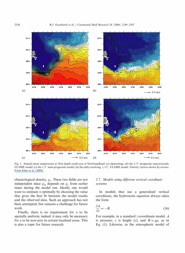
Sheng et al. (2001) applied the standard methodto a limited area model of the northwest AtlanticOcean. The use of the semi-prognostic method ledto a dramatic improvement in the model perfor-mance, especially in the representation of the GulfStream and the ‘‘northwest corner’’ to the south-east of Newfoundland. Particularly pleasing is theimprovement in the unconstrained potential tem-perature, y; and salinity, S, fields. One by-productis that the magnitude of the semi-prognosticcorrection, which depends on the differencebetween the model ym;Sm-fields and the inputclimatology, yc;Sc; is much less than would besupposed by directly comparing the y;S-fieldsfrom the prognostic model run with the climatol-ogy (see Fig. 1).

In their calculations, Sheng et al. put a ¼ 0:5;although they also note that the model results arenot sensitive to choosing a in the range 0:4 to 0:6:Sheng et al. argued that a ¼ 0:5 is a reasonablechoice based on the so-called best linear unbiasedestimator (BLUE) method. BLUE can be used tooptimally blend two independent model runs. InSheng et al., the diagnostic and prognostic modelruns are taken as being independent, and themodel velocities on the eastern Canadian shelfcompared with the inventory of current meter dataheld at the Bedford Institute of Oceanography.The error variance based in the difference betweenmonthly mean model (in Year 2) and observedcurrents is found to be about the same for both thediagnostic and prognostic model runs. BLUE canthen be used to argue that the two models can beblended with equal weights. However, a difficultyin trying to apply BLUE to a semi-prognosticmodel is that in Eq. (2), it is the instantaneousmodel density, rm; that is ‘‘blended’’ with the

ARTICLE IN PRESS

0.5 m/s

0.5 m/s0.5 m/s

(a) (b)

(c) (d)

Fig. 1. Annual mean temperature at 50m depth south-east of Newfoundland: (a) climatology; (b) the 1=3� prognostic (uncorrected),

FLAME model; (c) the 1=3� semi-prognostic model; (d) the eddy-resolving, 1=12�; FLAME model. Velocity vectors shown by arrows.

From Eden et al. (2004).

R.J. Greatbatch et al. / Continental Shelf Research 24 (2004) 2149–21652156

climatological density, rc: These two fields are notindependent since rm depends on rc from earliertimes during the model run. Ideally one wouldwant to estimate a optimally by choosing the valuethat gives the best fit between the model resultsand the observed data. Such an approach has notbeen attempted, but remains a challenge for futurework.

Finally, there is no requirement for a to bespatially uniform; indeed, it may only be necessaryfor a to be non-zero in certain localised areas. Thisis also a topic for future research.

2.7. Models using different vertical coordinate

systems

In models that use a generalised verticalcoordinate, the hydrostatic equation always takesthe form

@A

@s¼ �R: (16)

For example, in a standard z-coordinate model, A

is pressure, s is height (z), and R ¼ gr; as inEq. (1). Likewise, in the atmospheric model of

ARTICLE IN PRESS

R.J. Greatbatch et al. / Continental Shelf Research 24 (2004) 2149–2165 2157

Hoskins and Simmons (1975), A is geopotentialheight, s is lnðsÞ and R ¼ T ; where T is tempera-ture and s is pressure normalised by the surfacepressure. In a model that uses density as its verticalcoordinate (e.g. MICOM—see Bleck and Boudra,1981), A is the Montgomery potential and R is thegeopotential. In all these cases, the semi-prognos-tic method can be applied exactly as describedabove; that is by replacing (16) by

@A

@s¼ �aRm � ð1� aÞRc: (17)

When the input data is from a climatological dataset, it is important that Rc has been averaged in thesame coordinate system as the model. So, forexample, if the semi-prognostic method is appliedto the atmospheric model of Hoskins and Sim-mons (1975), the input temperature climatology,Tc; should consist of temperature data that hasbeen averaged in the normalised-pressure coordi-nate system used by the model. Likewise, forapplication to the MICOM model, the input datashould be the geopotential height averaged onconstant density surfaces.

3. Applications of the method

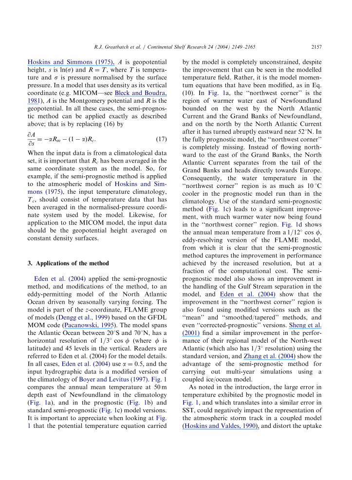
Eden et al. (2004) applied the semi-prognosticmethod, and modifications of the method, to aneddy-permitting model of the North AtlanticOcean driven by seasonally varying forcing. Themodel is part of the z-coordinate, FLAME groupof models (Dengg et al., 1999) based on the GFDLMOM code (Pacanowski, 1995). The model spansthe Atlantic Ocean between 201S and 701N, has ahorizontal resolution of 1=3� cos f (where f islatitude) and 45 levels in the vertical. Readers arereferred to Eden et al. (2004) for the model details.In all cases, Eden et al. (2004) use a ¼ 0:5; and theinput hydrographic data is a modified version ofthe climatology of Boyer and Levitus (1997). Fig. 1compares the annual mean temperature at 50mdepth east of Newfoundland in the climatology(Fig. 1a), and in the prognostic (Fig. 1b) andstandard semi-prognostic (Fig. 1c) model versions.It is important to appreciate when looking at Fig.1 that the potential temperature equation carried

by the model is completely unconstrained, despitethe improvement that can be seen in the modelledtemperature field. Rather, it is the model momen-tum equations that have been modified, as in Eq.(10). In Fig. 1a, the ‘‘northwest corner’’ is theregion of warmer water east of Newfoundlandbounded on the west by the North AtlanticCurrent and the Grand Banks of Newfoundland,and on the north by the North Atlantic Currentafter it has turned abruptly eastward near 521N. Inthe fully prognostic model, the ‘‘northwest corner’’is completely missing. Instead of flowing north-ward to the east of the Grand Banks, the NorthAtlantic Current separates from the tail of theGrand Banks and heads directly towards Europe.Consequently, the water temperature in the‘‘northwest corner’’ region is as much as 10 1Ccooler in the prognostic model run than in theclimatology. Use of the standard semi-prognosticmethod (Fig. 1c) leads to a significant improve-ment, with much warmer water now being foundin the ‘‘northwest corner’’ region. Fig. 1d showsthe annual mean temperature from a1=12� cos f;eddy-resolving version of the FLAME model,from which it is clear that the semi-prognosticmethod captures the improvement in performanceachieved by the increased resolution, but at afraction of the computational cost. The semi-prognostic model also shows an improvement inthe handling of the Gulf Stream separation in themodel, and Eden et al. (2004) show that theimprovement in the ‘‘northwest corner’’ region isalso found using modified versions such as the‘‘mean’’ and ‘‘smoothed/tapered’’ methods, andeven ‘‘corrected-prognostic’’ versions. Sheng et al.(2001) find a similar improvement in the perfor-mance of their regional model of the North-westAtlantic (which also has 1=3� resolution) using thestandard version, and Zhang et al. (2004) show theadvantage of the semi-prognostic method forcarrying out multi-year simulations using acoupled ice/ocean model.

As noted in the introduction, the large error intemperature exhibited by the prognostic model inFig. 1, and which translates into a similar error inSST, could negatively impact the representation ofthe atmospheric storm track in a coupled model(Hoskins and Valdes, 1990), and distort the uptake

ARTICLE IN PRESS

R.J. Greatbatch et al. / Continental Shelf Research 24 (2004) 2149–21652158

of tracers by the ocean model. As noted by Eden etal. (2004), the error in SST leads to a region of heatuptake by the ocean model in the ‘‘northwestcorner’’ region. This region of heat uptake is notfound in heat flux products generated by atmo-spheric models, but is a common feature in heatfluxes generated by ocean models due to thesystematic error in the path of the North AtlanticCurrent.

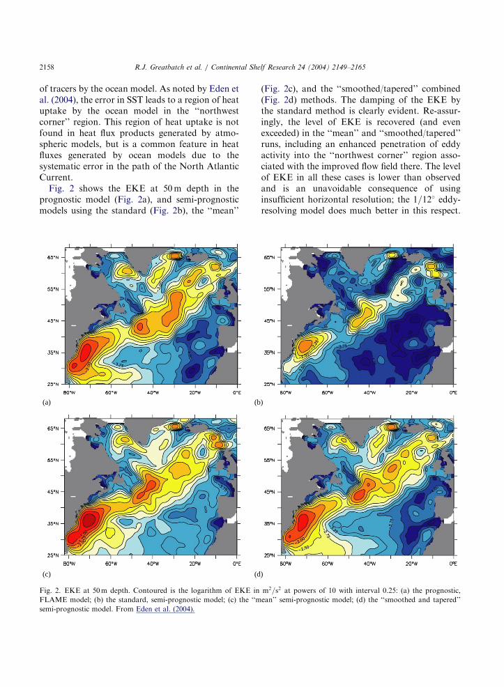
Fig. 2 shows the EKE at 50m depth in theprognostic model (Fig. 2a), and semi-prognosticmodels using the standard (Fig. 2b), the ‘‘mean’’

(a) (b

(c) (d

Fig. 2. EKE at 50m depth. Contoured is the logarithm of EKE in

FLAME model; (b) the standard, semi-prognostic model; (c) the ‘‘m

semi-prognostic model. From Eden et al. (2004).

(Fig. 2c), and the ‘‘smoothed/tapered’’ combined(Fig. 2d) methods. The damping of the EKE bythe standard method is clearly evident. Re-assur-ingly, the level of EKE is recovered (and evenexceeded) in the ‘‘mean’’ and ‘‘smoothed/tapered’’runs, including an enhanced penetration of eddyactivity into the ‘‘northwest corner’’ region asso-ciated with the improved flow field there. The levelof EKE in all these cases is lower than observedand is an unavoidable consequence of usinginsufficient horizontal resolution; the 1=12� eddy-resolving model does much better in this respect.

)

)

m2=s2 at powers of 10 with interval 0.25: (a) the prognostic,

ean’’ semi-prognostic model; (d) the ‘‘smoothed and tapered’’

ARTICLE IN PRESS

10 0 10 20 30 40 50 600

0.1

0.2

0.3

0.4

0.5

0.6

0.7

0.8

0.9

1

Fig. 4. Northward heat transport in PW (ordinate) as a

function of latitude (abscissa) using modified versions of the

semi-prognostic method. Results from the corresponding

‘‘corrected-prognostic’’ versions are shown by the dashed lines,

and are almost indistinguishable. Red is for the ‘‘mean’’

method, blue for the ‘‘mean+smoothed+tapered’’ method,

and magenta is for the ‘‘mean+smoothed+tapered’’ method,

but with the correction applied only above 800m depth. From

Eden et al. (2004).

R.J. Greatbatch et al. / Continental Shelf Research 24 (2004) 2149–2165 2159

On the other hand, the horizontal distribution ofnear surface EKE is in general agreement withobservational estimates (Stammer et al., 1996).

Fig. 3 shows the poleward heat transport as afunction of latitude in the standard semi-prognos-tic model, the prognostic version of the samemodel, the eddy resolving (1=12�) model, and the1=3� model used for the DYNAMO modelintercomparison study (Willebrand et al., 2001).Also shown for comparison are estimates based onobservations. Disappointingly, the standard semi-prognostic model has the weakest and mostunrealistic heat transport of all the cases shown.As noted by Eden et al., the standard semi-prognostic method being used here is causing ashortcut in the meridional overturning circulationassociated with spurious upwelling at the latitudeof the Gulf Stream separation. The problemresults from a mismatch between the input densityfield, rc; and the model bottom topography,leading to spurious vertical velocities and anenhanced ‘‘Veronis effect’’ (Boning et al., 1995).The problem is cured by using the tapered method.This is illustrated in Fig. 4 which shows the

10 0 10 20 30 40 50 600

0.2

0.4

0.6

0.8

1

1.2

1.4

Fig. 3. Northward heat transport in PW (ordinate) as a

function of latitude (abscissa) in the eddy-permitting prognostic

model (black line), the DYNAMO model (red line), the eddy-

resolving, 1=12� model (green line), and the standard, semi-

prognostic model (blue line). Also shown are observational

estimates of oceanic heat transports given by MacDonald and

Wunsch (1996) (black circles and error bars), Ganachaud and

Wunsch (2000) (red circles and error bars) and by Trenberth

and Caron (2001) (dashed, magenta line). 1PW ¼ 1015 W:From Eden et al. (2004).

poleward heat transport when modified versions ofthe semi-prognostic method are used (including‘‘corrected-prognostic’’ model versions). This timeonly the ‘‘mean’’, and the ‘‘mean, corrected-prognostic’’ versions show the reduced heattransport, these being the two cases shown in thefigure that do not use tapering, while the othercases all give heat transports comparable to thatfrom the 1=12� eddy-resolving model shown inFig. 3.

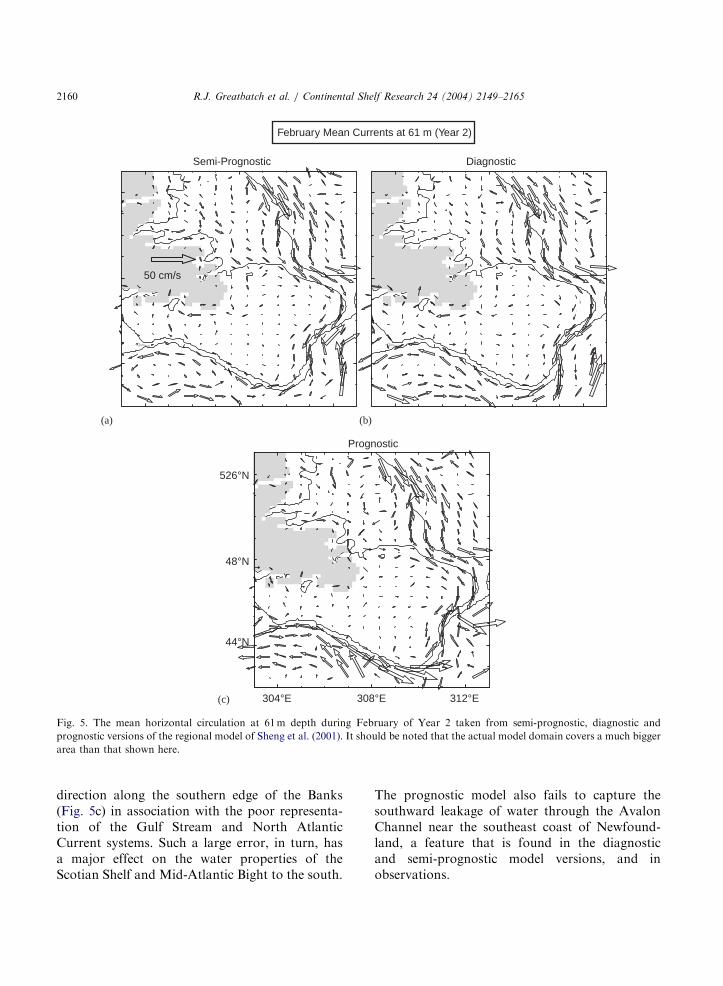
Finally in this section, Fig. 5 compares thehorizontal flow field in diagnostic, prognostic andstandard semi-prognostic versions of the regionalmodel of Sheng et al. (2001), showing thecirculation over and around the Grand Banks ofNewfoundland (the actual model domain is con-siderable bigger than the region shown in thefigure). In the diagnostic and semi-prognosticmodels, the offshore branch of the LabradorCurrent follows the shelf break around the Banksand feeds southwestward to the Scotian shelf,much as observed (e.g. Loder et al., 1998). Theprognostic model, on the other hand, is seriouslyin error, with flow in the opposite (incorrect)

ARTICLE IN PRESS

February Mean Currents at 61 m (Year 2)

Semi-Prognostic Diagnostic

Prognostic

50 cm/s

526°N

48°N

44°N

304°E 308°E 312°E

(a) (b)

(c)

Fig. 5. The mean horizontal circulation at 61m depth during February of Year 2 taken from semi-prognostic, diagnostic and

prognostic versions of the regional model of Sheng et al. (2001). It should be noted that the actual model domain covers a much bigger

area than that shown here.

R.J. Greatbatch et al. / Continental Shelf Research 24 (2004) 2149–21652160

direction along the southern edge of the Banks(Fig. 5c) in association with the poor representa-tion of the Gulf Stream and North AtlanticCurrent systems. Such a large error, in turn, hasa major effect on the water properties of theScotian Shelf and Mid-Atlantic Bight to the south.

The prognostic model also fails to capture thesouthward leakage of water through the AvalonChannel near the southeast coast of Newfound-land, a feature that is found in the diagnosticand semi-prognostic model versions, and inobservations.

ARTICLE IN PRESS

R.J. Greatbatch et al. / Continental Shelf Research 24 (2004) 2149–2165 2161

4. Use of the semi-prognostic method as a nested-

modelling technique

In this section we briefly describe the use of thesemi-prognostic method as a means of transferringinformation between the different submodelscomprising a nested modelling system. Often,detailed small-scale information is required withina limited area domain (e.g. in support of the oiland gas industry on the shelf), and it makes senseto nest a high-resolution, inner model inside acoarser-resolution, outer model. Sometimes, also,a model domain may contain choke points (e.g.the Gulf Stream separation region) where veryhigh resolution would be an advantage, eventhough such high resolution is not necessary overthe rest of the domain. The use of a two-waynested modelling system may then be desirable,with the inner, high-resolution model feeding backinformation to the coarser-resolution outer model.

A difficulty in developing a two-way nestingscheme is the compatibility problem (e.g., massconservation) at the grid interface (Ginis et al.,1998). Furthermore, undesirable numerical noisemay result from the change of the grid resolutionat the grid interface and an additional damping isrequired (Fox and Maskell, 1995). Kurihara et al.(1979) proposed a nesting technique in whichinformation is exchanged between the two modelsin a narrow zone (dynamic interface) near the gridinterface. The Kurihara et al. (1979) scheme hasbeen successfully applied to the ocean by Ginis etal. (1998). An alternative nesting technique devel-oped by Oey and Chen (1992) is to embed a finegrid (inner model) inside a coarse grid (outermodel) and use the inner model variables toupdate the outer model variables over the sub-region where the two grids overlap. Oey andChen’s scheme has the advantage of allowing atwo-way interaction not only at the grid interfacebut also directly inside the common subregionwhere the two grids overlap.

The use of the semi-prognostic method as anesting technique is illustrated below (more detailcan be found in Zhai et al., 2004). In the semi-prognostic approach, the focus is not on theexchange of information around the boundaries ofthe inner model, but rather on the exchange of

information between the inner and outer modelswithin the interior of the inner model domain.Indeed, in the applications shown in Fig. 6, there isnothing special about the treatment of the openboundaries of the inner model (the treatment is, infact, the same as in Sheng et al. (2001), but usingouter model output rather than climatologicaldata as input). As illustrated in Fig. 6 (see below),a virtue of the semi-prognostic method is its abilityto keep the inner model ‘‘on track’’ with the outermodel (and vica versa). But perhaps the principaladvantage of the semi-prognostic method overother nesting techniques is its simplicity and easeof implementation.

For the examples shown in Fig. 6, the outermodel is the same as that described in Sheng et al.(2001) and has roughly 25 km resolution, while theinner model has the domain shown in the figure,and has a resolution of roughly 7 km. Climatolo-gical, seasonally varying forcing is used, as inSheng et al. (2001). (The use of the same nestedmodelling system to simulate the passage of asevere storm over the shelf is described in Zhai(2004).) In the COW (Conventional One-Waynesting) case, the inner model is connected to theouter model only through the specification of theopen boundary conditions for the inner model,these being taken from the outer model. In theOSP (Original Semi-Prognostic) case, in additionto applying open boundary conditions to the innermodel as in the COW case, information is alsotransferred between the interiors of the modelsusing the version of the semi-prognostic methoddescribed in Sheng et al. (2001); that is usingEq. (2),

@p

@z¼ �g½arm þ ð1� aÞrc; (18)

where rm is the instantaneous model densityvariable and rc is now the density carried by theother submodel over their common domain (in thiscase, the domain of the high-resolution submodel).In two-way nesting (used to produce Fig. 6),Eq. (18) is used to transfer information from boththe outer to the inner model, and back again, fromthe inner to the outer model. (The method can alsobe used for one-way nesting, in which case thefeedback from the inner to the outer model is

ARTICLE IN PRESS

OUTER

OSP COW

SSP

0 5 10 15 20 25 30 35100 cm/s

(z = 50m) (z = 50m)

(z = 50m)(z = 50m)

(a) (b)

(c) (d)

Fig. 6. An instantaneous snapshot over the inner model domain of the temperature (gray image, �C) and horizontal velocity (arrows)

at 50m depth produced by (a) the outer model and (b) the inner model using the SSP nesting technique; (c) the inner model using the

OSP nesting technique and (d) the conventional one-way nested inner model. Velocity vectors are plotted at every four model grid

points for the inner model and every two model grid points for the outer model. From Zhai et al. (2004).

R.J. Greatbatch et al. / Continental Shelf Research 24 (2004) 2149–21652162

suppressed). Writing Eq. (18) as

@p

@z¼ �grm þ gð1� aÞðrm � rcÞ; (19)

the term gð1� aÞðrm � rcÞ is clearly the termresponsible for the information transfer betweenthe models. In the smoothed semi-prognostic(SSP) case, this term is smoothed spatially, as inthe ‘‘smoothed’’ method described Section 2.5. Forthe case shown in Fig. 6, the correction termapplied to the inner model is smoothed over 16

grid points (that is 112 km) so that inner modelfeels the outer model only on large spatial scales.(One consequence of this is that physical processesthat are captured by the inner model on scales lessthan 112 km will not be adversely affected by thenesting procedure). On the other hand, no spatialfiltering is applied to the correction term felt by theouter model.

The most striking feature of the instantaneoussnapshots shown in Fig. 6 is the very different flowfield in the COW case compared to both the outer

ARTICLE IN PRESS

R.J. Greatbatch et al. / Continental Shelf Research 24 (2004) 2149–2165 2163

model and also the SSP and OSP cases. Thisdifference is quite systematic and is also present intime-averaged fields (see Zhai et al., 2004). Indeed,in the COW case, the flow field within the innermodel domain has drifted away from that in theouter model, even though the outer model is usedto provide the boundary conditions for the innermodel. The result is that the Gulf Stream is too farto the north and is banked up against thecontinental slope in an unrealistic fashion. In theOSP and SSP cases, on the other hand, whereinformation is being exchanged between the innerand outer models in the interior of the inner modeldomain, the flow field is quite similar to that in theouter model, showing the usefulness of the semi-prognostic method for keeping the inner model ontrack with the outer model (and vica-versa whenthere is two-way nesting, as here). The greaterdetail apparent in the SSP case illustrates theadvantage of using the smoothed method in orderto gain the full advantage of the higher resolutionused in the inner model. For an example of thenesting technique applied to the Caribbean Sea,readers are referred to Sheng and Tang (2004).

5. Summary and discussion

In the preceding sections, we have reviewed thesemi-prognostic method, as it appeared in Sheng etal. (2001) and as subsequently modified by Eden etal. (2004). The method was introduced by Sheng etal. (2001) as a technique for adjusting hydrostaticocean models to correct for systematic error. Theresults shown in Sheng et al. (2001), Eden et al.(2004) and in Section 3 of this paper confirm thesuccess of the method, on both the regional (theeastern Canadian shelf, northwest Atlantic) andthe basin (North Atlantic Ocean) scale. What isparticularly pleasing is the improvement in themodelled temperature and salinity fields, despitethe fact the tracer equations carried by the modelare completely unmodified by the method. Rather,the correction is applied to the horizontal mo-mentum equations, with the advantage that themethod is adiabatic. The semi-prognostic methodcan be contrasted with the robust diagnosticmethod of Sarmiento and Bryan (1982), in which

sources and sinks are added to model’s potentialtemperature and salinity equations, making thatmethod highly diabatic. Adiabaticity, on the otherhand, ensures (i) that there is no compromise tothe requirement that the flow be primarily in theneutral tangent plane in the ocean interior, and (ii)that the method is well-suited for use in tracerstudies (e.g. Zhao et al., 2004). The semi-prog-nostic method is also easy to implement in modelcode, since all that is required is to adjust thedensity that is used in the model’s hydrostaticequation (see Section 2.7 for models that do notuse height coordinates in the vertical).

We noted in Section 2, that the standard methodused by Sheng et al. (2001) distorts the modeldynamics by reducing wave propagation speedsand damping the mesoscale eddy field. Themodified methods introduced by Eden et al.(2004) overcome these drawbacks, while maintain-ing the benefits of the standard method (seeSections 2.4 and 2.5 for the details). We alsonoted that Eden and Greatbatch (2003) turn thedistortion to advantage by using it to diagnose theimportant dynamical processes in a model of theNorth Atlantic Ocean.

The semi-prognostic method is a technique fortransferring information into and between models.As such, it is really a data assimilation technique.The adiabaticity of the semi-prognostic methodpoints to a certain kinship with the assimilationscheme of Cooper and Haines (1996). Theseauthors describe a method for assimilating satellitealtimeter data into a model that involves applyinguniform vertical displacements to the model’ssubsurface isopycnals. As such, the Cooper andHaines method preserves water mass properties aswell as the (planetary geostrophic) potentialvorticity field on isopycnal surfaces, two propertiesit shares with the semi-prognostic method. It isinteresting to speculate on the use of the semi-prognostic method as tool for ocean data assim-ilation. For example, the displaced isopycnal fieldof Cooper and Haines could be taken as the inputhydrography, rc in Eq. (2). Clearly, the use of thesemi-prognostic method as an assimilation techni-que is a topic for future research. Further workis also required to perfect the use of thesemi-prognostic method as a nested modelling

ARTICLE IN PRESS

R.J. Greatbatch et al. / Continental Shelf Research 24 (2004) 2149–21652164

technique, as described in Section 4 (see Zhai et al.,2004), and on the modified methods described inSection 2.5 in a search for ways to further mitigatethe distortion to the model physics inherent in thestandard method (see Section 2.4). Another areawhere future research is required is in the choice ofthe parameter a (see Eq. (2)), a topic discussed inSection 2.6. In particular, it may not be necessaryfor a to be spatially uniform. Indeed, there areprobably parts of the model domain where we canput a ¼ 1; so that the model is purely prognostic inthose regions. The spatial distribution of the semi-prognostic correction term (see Eqs. (5) and (8))may also provide insight into model deficiencies,and may therefore provide useful information onhow to improve the model physics.

Acknowledgements

This work has been supported by funding fromNSERC, CFCAS and CICS in support of theCanadian CLIVAR Research Network and byNSERC, MARTEC (a Halifax based company)and the Meteorological Service of Canada (MSC)in support of the NSERC/MARTEC/MSC In-dustrial Research Chair. Conversations with ClausBoning, Klaus Fraedrich, Chris Hughes, YouyuLu, Frank Lunkeit, Andreas Oschlies, DrewPeterson, Jurgen Willebrand and Dan Wrighthelped clarify our thinking about the semi-prog-nostic method and are gratefully acknowledged.Comments from two anonymous referees werehelpful when revising the manuscript. We are alsograteful to the MSC for the use of supercomputerfacilities at the Canadian Meteorological Centre inDorval, Quebec.

References

Bleck, R., Boudra, D.B., 1981. Initial testing of a numerical

ocean circulation model using a hybrid (quasi-isopycnic)

vertical coordinate. Journal of Physical Oceanography 11,

755–770.

Boning, C.W., Holland, W.R., Bryan, F.O., Danabasoglu, G.,

McWilliams, J.C., 1995. Deep-water formation and mer-

idional overturning in a high resolution model of the North

Atlantic. Journal of Climate 8, 515–523.

Boyer, T.P., Levitus, S., 1997. Objective analyses of tempera-

ture and salinity for the world ocean on a 1=4� grid.

Technical Report, NOAA Atlas NESDIS 11, US Govern-

ment Printing Office, Washington DC, USA.

Cooper, M., Haines, K., 1996. Altimetric assimilation with

water property conservation. Journal of Geophysical

Research 101, 1059–1077.

Dengg, J., Boning, C.W., Ernst, U., Redler, R., Beckmann, A.,

1999. Effects of an improved model representation of

overflow water on the subpolar North Atlantic. WOCE

Newsletter 37.

Dewar, W.K., Hsueh, Y., McDougall, T.J., Yuan, D., 1998.

Calculation of pressure in ocean simulations. Journal of

Physical Oceanography 28, 577–588.

Eden, C., Greatbatch, R.J., 2003. A damped, decadal oscilla-

tion in the North Atlantic climate system. Journal of

Climate 16, 4043–4060.

Eden, C., Greatbatch, R.J., Boning, C.W., 2004. Adiabatically

correcting an eddy-permitting model using large-scale

hydrographic data: application to the Gulf Stream and the

North Atlantic Current. Journal of Physical Oceanography

34, 701–719.

Fox, A.D., Maskell, S.J., 1995. Two-way interactive nesting of

primitive equation ocean models with topography. Journal

of Physical Oceanography 25, 2977–2996.

Ganachaud, A., Wunsch, C., 2000. Improved estimates of

global ocean circulation, heat transport and mixing from

hydrographic data. Nature 408, 453–457.

Gill, A.E., 1982. Atmosphere-Ocean Dynamics. Academic

Press, San Diego, CA, 662pp.

Ginis, I., Richardson, A., Rothstein, L., 1998. Design of a

multiply nested primitive equation ocean model. Monthly

Weather Review 126, 1054–1079.

Greatbatch, R.J., 1998. Exploring the relationship between

eddy-induced transport velocity, vertical mixing of momen-

tum and the isopycnal flux of potential vorticity. Journal of

Physical Oceanography 28, 422–432.

Greatbatch, R.J., 2000. The North Atlantic Oscillation.

Stochastic Environmental Research and Risk Assessment

14, 213–242.

Greatbatch, R.J., Lamb, K.G., 1990. On parameterizing

vertical mixing of momentum in non-eddy-resolving ocean

models. Journal of Physical Oceanography 20, 1634–1637.

Greatbatch, R.J., McDougall, T.J., 2003. The non-Boussinesq

temporal-residual-mean. Journal of Physical Oceanography

33, 1231–1239.

Greatbatch, R.J., Mellor, G.L., 1999. An overview of coastal

ocean models. In: Mooers, C.N.K. (Ed.), Coastal Ocean

Prediction, American Geophysical Union, Coastal and

Estuarine Studies 56, 31–57.

Greatbatch, R.J., Fanning, A.F., Goulding, A., Levitus, S.,

1991. A diagnosis of interpentadal circulation changes in the

North Atlantic. Journal of Geophysical Research 96,

22009–22023.

Gregg, M.C., 1989. Scaling turbulent dissipation in the

thermocline. Journal of Geophysical Research 94,

9686–9698.

ARTICLE IN PRESS

R.J. Greatbatch et al. / Continental Shelf Research 24 (2004) 2149–2165 2165

Holloway, G., 1992. Representing topographic stress for large-

scale ocean models. Journal of Physical Oceanography 22,

1033–1046.

Hoskins, B.J., Simmons, A.J., 1975. A multi-layer spectral

model and the semi-implicit method. Quarterly Journal of

the Royal Meteorological Society 101, 637–655.

Hoskins, B.J., Valdes, P.J., 1990. On the existence of storm-

tracks. Journal of Atmospheric Sciences 47, 1854–1864.

Hurrell, J.W., Kushnir, Y., Ottersen, G., Visbeck, M., 2003. An

overview of the North Atlantic Oscillation. In: Hurrell, J.W.,

Kushnir, Y., Ottersen, G., Visbeck, M. (Eds.), The North

Atlantic Oscillation: Climatic Significance and Environmen-

tal Impact, AGU Geophysical Monograph 134, 1–35.

Kurihara, Y., Tripoli, G.J., Bender, M.A., 1979. Design of a

movable nested-mesh primitive equation model. Monthly

Weather Review 107, 239–249.

Lazier, J.R.N., 1994. Observations in the northwest corner of

the North Atlantic Current. Journal of Physical Oceano-

graphy 24, 1449–1463.

Ledwell, J.R., Watson, A.J., Law, C.S., 1998. Mixing of a tracer

in the pycnocline. Journal of Geophysical Research 103,

21499–21529.

Loder, J.W., Petrie, B., Gawarkiewicz, G., 1998. The coastal

ocean off northeastern North America: a large-scale view.

In: Robinson, A.R., Brink, K.H. (Eds.), The Sea, vol. 11.

Wiley, New York, pp. 105–133.

MacDonald, A.M., Wunsch, C., 1996. An estimate of global

ocean circulation and heat fluxes. Nature 382, 436–439.

McDougall, T.J., 1987. Neutral surfaces. Journal of Physical

Oceanography 17, 1950–1964.

Mertz, G., Wright, D.G., 1992. Interpretations of the JEBAR

term. Journal of Physical Oceanography 22, 301–305.

Oey, L.Y., Chen, P., 1992. A nested-grid ocean model: with

application to the simulation of meanders and eddies in the

Norwegian Coastal Current. Journal of Geophysical Re-

search 97, 20063–20086.

Oschlies, A., Willebrand, J., 1996. Assimilation of Geosat

altimeter data into an eddy-resolving primitive equation

model of the North Atlantic Ocean. Journal of Geophysical

Research 101, 14,175–14,190.

Pacanowski, R.C., 1995. MOM-2 Documentation, User’s

Guide and Reference Manual. Technical Report, GFDL

Ocean Group, GFDL, Princeton, USA.

Sarmiento, J.L., Bryan, K., 1982. An ocean transport model for

the North Atlantic. Journal of Geophysical Research 87,

394–408.

Sheng, J., Tang, L., 2004. A two-way nested-grid ocean

circulation model for the Meso-American Barrier Reef

System. Ocean Dynamics, 54, 10.1007/s10236-003-0074-3,

232–242.

Sheng, J., Greatbatch, R.J., Wright, D.G., 2001. Improving the

utility of ocean circulation models through adjustment of

the momentum balance. Journal of Geophysical Research

106, 16711–16728.

Stammer, D., Tokmakian, P.R., Semtner, A., Wunsch, C.,

1996. How well does a 1/4 deg global model simulate large-

scale oceanic observations? Journal of Geophysical Re-

search 101, 25779–25811.

Sundermeyer, M.A., Ledwell, J.R., 2001. Lateral disper-

sion over the continental shelf: analysis of dye-release

experiments. Journal of Geophysical Research 106,

9603–9622.

Trenberth, K., Caron, J., 2001. Estimates of meridional

atmosphere and ocean heat transports. Journal of Climate

14, 3433–3443.

Willebrand, J., Barnier, B., Boning, C.W., Dieterich, C.,

Killworth, P., LeProvost, C., Jia, Y., Molines, J.M., New,

A.L., 2001. Circulation characteristics in three eddy-

permitting models of the North Atlantic. Progress in

Oceanography 48, 123–161.

Woodgate, R., Killworth, P., 1997. The effect of assimilation on

the physics of an ocean model. Part I: theoretical model and

barotropic results. Journal of Atmospheric and Oceanic

Technology 14, 897–909.

Zhai, X., 2004. Studying storm-induced circulation on the

Scotian Shelf and slope using a two-way nested-grid model.

M.Sc. Thesis, Department of Oceanography, Dalhousie

University, Halifax, Nova Scotia, Canada.

Zhai, X., Sheng, J., Greatbatch, R.J., 2004. A new two-way

nested-grid ocean modelling technique applied to the

Scotian Shelf and Slope Water. Proceedings of the Eighth

International Conference on Estuarine and Coastal Model-

ing, in press.

Zhang, S., Sheng, J., Greatbatch, R.J., 2004. A coupled ice-

ocean modelling study of the northwest Atlantic Ocean.

Journal of Geophysical Research, 109, C04009, 10.1029/

2003JC001924.

Zhao, J., Greatbatch, R.J., Sheng, J., Eden, C., Azestu-Scott,

K., 2004. Impact of an adiabatic correction technique on the

simulation of CFC-12 in a model of the North Atlantic

Ocean. Geophysical Research Letters 31, L12309, 10.1029/

2004GL020206.