Extension of the zonal method to inhomogeneous non-grey semi-transparent medium

This article appeared in a journal published by Elsevier. The attachedcopy is furnished to the author for internal non-commercial researchand education use, including for instruction at the authors institution

and sharing with colleagues.

Other uses, including reproduction and distribution, or selling orlicensing copies, or posting to personal, institutional or third party

websites are prohibited.

In most cases authors are permitted to post their version of thearticle (e.g. in Word or Tex form) to their personal website orinstitutional repository. Authors requiring further information

regarding Elsevier’s archiving and manuscript policies areencouraged to visit:

http://www.elsevier.com/copyright

http://www.elsevier.com/copyright

Author's personal copy

Extension of the zonal method to inhomogeneous non-greysemi-transparent medium

Rachid Mechi a, Habib Farhat a,*, Kamel Guedri a, Kamel Halouani b, Rachid Said a

a Unite de Recherche Etude des Milieux Ionises et Reactifs (EMIR), Rue Ibn El Jazzar, 5019 Monastir, Tunisieb METS–ENIS–IPEIS, Route Menzel Chaker, B.P. 805, 3000 Sfax, Tunisie

a r t i c l e i n f o

Article history:Received 22 February 2009Received in revised form17 June 2009Accepted 17 June 2009Available online 13 November 2009

Keywords:Exchange areasInhomogeneousNon-isothermalSemi-transparent mediumSmoothingWSGG modelZonal method

a b s t r a c t

A radiation model is proposed to extend the zonal method of Hottel to semi-transparent inhomogeneousreal combusting gas–soot mixture in a 2-D black-walled rectangular enclosure. The direct exchange areasare carried out by direct numerical integration and then adjusted to meet the conservation constraintsusing two smoothing processes namely the Larsen and Howell’s least squares and generalized Lawson’simproved smoothing methods, which has not been previously done to the best knowledge of the authors.The predicted net radiative heat flux distributions compare favorably with benchmark solutions for twotest cases dealing with isothermal and non-isothermal homogeneous mediums. It is concluded from thisinvestigation that there is no significant effect of the smoothing method on the computed wall heatfluxes for the homogeneous and inhomogeneous test cases using different grey gases number. The griddependence study depicts that the numerical solutions fully achieve grid independence. It is worthnoting that it can be proceeded with the present extended zonal method and computer code to morecomplex cases. The results based on the generalized Lawson’s smoothing method compare favorablywith those yielded by the popular least squares method and, consequently, can be considered asa benchmark solution for other investigations.

� 2009 Published by Elsevier Ltd.

1. Introduction

In many thermal industrial processes such as boilers andfurnaces or other gas-fired combustion systems, radiation heattransfer plays an important role in over all heat transfer. The heattransfer process in such participating media is described using theRTE (radiative transfer equation). Thus, for a wide range ofcombustion situations with non-uniform mixtures of soot and gasin a non-isothermal field, solution of the RTE is difficult due to itsspectral and angular dependency so that no analytical solution ishandled. Therefore, some approximated solution methods aredeveloped in the last decades taking into account the multi-dimensional geometries, anisotropically scattering media [1,2], andnon-grey behaviour of both the gaseous combustion products andsurrounding walls [3,4] allowing the simulation of the gas radiativeproperties in sooting non-grey and inhomogeneous participatingmedia.

The radiative heat transfer was always a challenge for theengineers and researchers who attempted for many years toprovide accurate solutions of the RTE through many developedsolution methods. Among the most powerful numerical tools, thezoning method due to Hottel and Cohen [5] and Hottel and Sarofim[6] has been widely used as a solution for the RTE in many practicalengineering calculations. The radiating gaseous combustion prod-ucts in the most industrial natural-gas or fuel combustion furnacesare mainly the CO2 (carbon dioxide) and the H2O (water vapour).Several studies have thoroughly dealt with heat transfer in indus-trial processes intervening H2O such as the steam generators [7,8].When the H2O is over-heated, it is regarded as a non-grey gas dueto its large absorption bands [7]. Recently, entropy generation studyhas been achieved in two parallel plates between them a laminarflow of H2O is maintained at high temperature [7]. The radiativepart of this investigation has been performed with the ray tracingmethod through S4 directions associated with the hybrid SNB-CK(statistical narrow band correlated-k) model taking into account,thus, the non-greyness of the over-heated steam.

Among the accurate spectral gas radiative properties models,the SNB (statistical narrow band) model and the WBM (wideband model) are the most known. These models achieve a good

* Corresponding author. Tel.: þ968 26720101x106; fax: þ968 26720102.E-mail addresses: [email protected] (R. Mechi), [email protected]

(H. Farhat), [email protected] (K. Guedri), [email protected](K. Halouani), [email protected] (R. Said).

Contents lists available at ScienceDirect

Energy

journal homepage: www.elsevier .com/locate/energy

0360-5442/$ – see front matter � 2009 Published by Elsevier Ltd.doi:10.1016/j.energy.2009.06.040

Energy 35 (2010) 1–15


approximation degree; however they are time consuming andconsequently not practical for engineering calculations.

On the other hand, good progress has been made in predictingradiation from isothermal mixtures of combustion products con-taining soot, CO2 and H2O of known composition. In this context,several non-grey gas models have been developed such as theModak’s gas emissivity model [9] for a homogeneous andisothermal CO2–H2O and soot mixture, Leckner’s model for firecombustion products [10] and Hottel’s WSGG (weighted sum ofgrey gases) model [6]. The latter require only available levels ofcomputing power but to the detriment of accuracy. The theoreticalbasis exists for extending these models to the more realistic non-isothermal combustion situations as that due to Grosshandler andModak [11], simple to apply for non-isothermal and inhomoge-neous gas–soot mixture. However, similarly convenient and generalmodels haven’t yet been developed. The object here is to developsuch a model, which is inexpensive and of proven accuracy, fortreating non-isothermal and non-grey mixtures of CO2, H2O and

soot. During the last decade, the WSGG model has been shown to bea good bridge between accuracy and computing time as comparedto the SNB and the correlated-k (C-K) distribution methods [11–13].The most used WSGG model parameters are those of Truelove [14],Farag [15], Smith et al. [16] and Soufiani and Djavdan [17].

The main goal of this study is to compare the current results,given by a 2-D computational code of radiation heat transfercalculations allowing the estimation of the normalized DEAs (directexchange areas) in isothermal and non-isothermal black-walledrectangular enclosure, with the benchmark solutions provided byGoutiere et al. [12] for two test case problems. Furthermore, theradiation model is extended to achieve flux calculations for inho-mogeneous gas–soot mixture with non-uniform radiative proper-ties. Therefore, the bilinear interpolation technique, taking intoaccount the spatial dependence of the gas–soot mixture absorptioncoefficient, has been introduced within a new numerical procedure.

The initial estimates of DEAs are computed by the so-calleddirect numerical integration and then enforced to meet the

Nomenclature

A area of a surface zone (m2)ag WSGG weighting factorsC mass soot concentration (kg m�3)d differentiation (Eqs. (2) and (13))E+ ¼sT4, blackbody emissive power (W m�2)fg, fs Murty’s constants (Eq. (29))i, I, j, J increments related to a given mesh, defining the

position of a discretized volume zone in x-directionand y-direction respectively

k, k� k number of subdivisions in a surface and volume zonesrespectively

kg specific absorption coefficient for a grey gas(m�1 atm�1)

ks specific absorption coefficient for soot (m2 kg�1)Kg grey gas absorption coefficient (m�1)Kt attenuation coefficient of the medium (m�1)L gas path length (m)M number of increments (or zones) in y-directionMx total number of surface and volume zones in the

enclosureN number of increments (or zones) in x-directionn! unit outward normal vector at a surface elementP gas partial pressure (atm)q total wall heat flux or wall heat flux per unit area (W/

W m�2)r distance between the centres of two zones (m)ss, sg and gg surface-to-surface, surface-to-gas and gas-to-gas

direct exchange areas respectively (m2)SiSj;GiSj surface-to-surface and gas-to-surface total exchange

areas respectively (m2)SiSj��!

;GiSj��!

surface-to-surface and gas-to-surface directed fluxareas respectively (m2)

s curvilinear coordinate (m)s’ integration variable (Eqs. (12), (23) and (25))T temperature (K)u, v spatial interpolation coefficientsV volume of a gas zone (m3)wij weighting coefficients used in the least squares

method[X] global matrix of direct exchange areas estimates for all

the types of radiative exchange

x, y coordinate directions (m)xij element from the matrix of the direct exchange areas

estimates (m2)xij0 element from the matrix of adjusted direct exchange

areas (m2)Dx, Dy the step of discretization along x and y directions,

respectively[ ] matrix

Greek symbolsan volumetric coefficient of interpolation (m�3) (Eqs. (18),

(19) and (23))bn squared gas–soot interpolated absorption coefficient

(m�2) (Eqs. (18), (19) and (23))gn interpolated gas–soot absorption coefficient (m�1)

(Eqs. (18), (19) and (23))G number of surface or volume zones3 total gas emissivityh, x direction cosinesq angle between the normal to a surface and the path

between the centre points in two surfaces (rad)l Lagrange multiplierm ¼cos q, direction cosines ¼5.67� 10�8 W m�2 K�4, Stefan–Boltzmann constants transmissivity for a given column gasU!

ray direction

Subscriptsg gasi, j, k surface or volume zonem mth zone subdivision elementn nth grey gas, zone subdivision element or entry point

of a ray crossed grid cellnþ 1 exit point of a ray crossed grid cells surface or soot

Superscripts+ blackbodyp, pþ 1 old and recent iteration respectivelyT matrix transpose0 smoothed exchange areas or revised estimates

R. Mechi et al. / Energy 35 (2010) 1–152


conservation constraints. For this purpose, the well known leastsquares method associated to the Lagrange multipliers [18] hasbeen used. Besides, the Lawson’s smoothing method [19], analternative to the Leersum’s algorithm [20], has been generalizedhereafter to the case of semi-transparent medium for the first timeto the best knowledge of the authors. Results of both iterativesmoothing processes are presented and discussed in each test caseproblem for different grey gases number and grid cells.

2. Mathematical radiation model

2.1. Introduction

Perhaps the most accurate method for calculating radiativetransfer in non-isothermal media and unusual geometries is thezone method as developed by Hottel and Cohen [5] and Hottel andSarofim [6]. Application of the zone method requires the whole gasvolume to be divided into a given number of smaller surfaces andvolumes with uniform properties such as temperature, composi-tion, emissivity and transmissivity. The basic idea of the zonemethod is to deal with DEAs for a grey gas. These grey gas exchangeareas are temperature-independent and are the basic ingredients inthe formulation of real-gas spectral models [6]. Physically, in thecase of an enclosure, the DEAs consider only direct radiantexchange between black surface zones and/or non-scatteringvolume zones. Alternatively, the TEAs (total exchange areas) alsoaccount for additional exchange between zone pairs arising frommultiple reflections on the walls and/or isotropic scatter fromintervening volume elements. The TEAs are explicit functions of theDEAs, albedo of the medium, and the emissivity profile of theenclosure [21]. Finally, allowance for non-grey gas behaviour iseffected by use of DFAs (directed flux areas). More details for theradiative pattern used in this work have been reported in a numberof surveys [22–28].

2.2. The WSGG model

The WSGG model has been initially developed by Hottel andSarofim within the framework of the zonal method [6]. Modest hasshown that this model may be extended to be used with any RTEsolution method [29]. The WSGG model consists in replacing thereal gas by a set of several virtual gas components, each one with itsown constant absorption coefficient. Through the choice of anappropriate set of weights and absorption coefficients, the radiativebehaviour of the hypothetical gas is made somewhat like the realgas. The WSGG model has drawn more and more survey amonginvestigators as a practical non-grey gas model owing to itssimplicity when incorporated in any RTE solution solvers, itsreasonable accuracy and relatively rapid execution time for theengineering applications. Recently, new mathematical models havebeen developed to handle radiative heat transfer in combustionsystems based on the concept of WSGG model [25,26,28,30]. Thetotal gas emissivity is obtained by summation of all the grey gasemissivities over a small number of grey gases. One of the latter,namely clear gas, has its absorption coefficient assigned zero valuein order to account for the windows in the spectrum between thespectral regions that have absorption. Two or three grey gases plusone clear gas are quite sufficient [12,13,17,23]. Thus, the total gasemissivity is given by [25,26,28]

3gðTÞ ¼X

nag;nðTÞ

h1� eKg;nL

i(1)

The weighting factors ag,n are temperature polynomialsobtained by fitting the total emissivity of emission/absorption

contributors (mainly CO2 and H2O in gas-fired combustionsystems) to those calculated by the EWB (exponential wide band)model or by other spectral models [14,16]. Kg,n is the absorptioncoefficient for the nth grey gas (Kg,n¼ kg,nP). For a gas mixture,P is the sum of the partial pressures of the radiatively absorbingspecies. The weighting factors ag,n and the specific grey gasabsorption coefficient kg,n are the WSGG model parameters[14–17,25,26].

The so-called WSGG model is a highly attractive and practicalnumerical tool to be used in the full modelling of gas-firedcombustion systems since the former is formulated in terms of theabsorption coefficient of radiating species. It is restricted to greywalled enclosures but for industrial problems this is usually anacceptable, even necessary, simplification [22]. Also, it is used topredict radiation heat transfer in semi-transparent medium con-taining CO2, H2O or mixture of these two species with knowncomposition.

In this paper, the most popular WSGG model parameters due toTruelove [14], Farag [15] and Smith et al. [16] are employed. Fora given grey gas absorption property Kg,n, the DEAs are estimatedbased on the Hottel’s zone method and the Olsommer et al’salternative [31]. Extension of this radiation model usually used inhomogeneous combustion configurations, to non-uniform mixtureof more realistic combustion products in different engineeringapplications, will be presented hereafter starting where twohomogenous test cases are considered.

2.3. The zoning method of Hottel

In the standard zone method, the enclosure is divided into gasand surface zones which are small enough to justify the assumptionthat the properties in each zone are uniform [6,23,31]. First, theDEAs are numerically estimated for each grey gas and thennormalized. The least squares associated to the Lagrange multi-pliers due to Larsen and Howell [18] and the improved Lawsonsmoothing method [19] are the most widely used smoothingmethods. The smoothed DEAs are stored as a set of data and used toevaluate the TEAs by matrix relations [6,21,31,32]. We notice thatthe TEAs are systematically normalized and don’t need to besmoothed. For a given grey gas absorption coefficient, the DEAs andTEAs are independent of the gas zone temperatures. Hence, theyneed only be assessed once for each single grey gas before solvingthe governing energy balance equations over all the surface andvolume zones. These equations are formulated for the radiationinterchanges between all surface-to-surface, surface-to-volume,volume-to-surface and volume-to-volume zones. The DEAs,expressed by the following multiple integrals, verify the reciprocityconditions [2,32]

8>>>>>>>>>>>>>>><>>>>>>>>>>>>>>>:

sisj ¼ZAi

ZAj

mimj e�Ktrij

pr2ij

dAi dAj ¼ sjsi

gisj ¼ZVi

ZAj

Ktmj e�Kt rij

pr2ij

dVi dAj ¼ sjgi

gigj ¼ZVi

ZVj

K2t e�Ktrij

pr2ij

dVi dVj ¼ gjgi

(2)

Physically, these exchange areas should obey the conservationconstraints or summation rules which are written for a surfacezone j [5]

R. Mechi et al. / Energy 35 (2010) 1–15 3


Xi

sjsi þX

i

sjgi ¼ Aj j ¼ 1;.;Gs (3)

and for a volume zone k

Xi

gksi þX

i

gkgi ¼ 4KtVk k ¼ 1;.;Gg (4)

In this work, the surface and volume zones are further subdividedinto smaller volume and surface elements. Then, the DEAs betweentwo finite surface or volume zones are evaluated with directnumerical integration by making a simple summation of the DEAsbetween these smaller elements [31,33,34]. With such numericaltechnique, DEAs are evaluated with inherent numerical errors.Since the eqs. (3) and (4) hold in the limit of zero numerical errors,smoothing methods may be indispensable to overcome thisdrawback. Also, with a finer grid cells, the direct numerical inte-gration yields sufficiently accurate results [31,32]. This method willbe detailed when treating the case of inhomogeneous media(Section 3.2.1).

The TEAs are deduced from the adjusted DEAs using someexplicit matrix relations [21,32,35]. Then, energy balances aredrawn up on each zone and a set of nonlinear algebraic equations ofunknown temperatures is obtained. The simultaneous solution ofthese equations allows the temperature distribution in the enclo-sure. Substitution of these temperatures into the energy equationsfor the surface zones enables the surface heat fluxes to be assessedintroducing the so-called DFAs [3]. The net radiative heat flux ona surface zone Ai may be specified as [3,23,25,31]

qi ¼XGs

j¼1

SjSi�!

E+s;j þ

XGg

j¼1

GjSi��!

E+g;j � Ai3iE

+s;i (5)

Es and Eg, in the right hand side of the eq. (5), are the blackbodyemissive powers of the surface zones and the gas zones respectivelywhereas SiSj

��!and GiSj

��!are the DFAs for surface-to-surface and gas-

to-surface radiative exchange respectively given by [3,25,31]

8>>><>>>:

SiSj�! ¼

Xn

ag;nðTiÞ�

SiSj

�Kg;n

GiSj��!

¼X

nag;nðTiÞ

�GiSj

�Kg;n

(6)

These temperature-dependent exchange areas are obtained bya simple summation of the TEAs over all the grey gases (a smallnumber of 3 or 4 grey gases is quite sufficient) weighted by thecoefficients ag,n which are polynomials on the local temperatures ofsurface or gas zones. Similar expressions of the DFAs can be writtenfor surface-to-gas and gas-to-gas radiative exchange [3,23,31].

2.4. Smoothing methods of DEA

2.4.1. LSSM (least squares smoothing method)Larsen and Howell [18] have suggested a least squares

smoothing procedure using Lagrange multipliers for adjusting theexchange areas in order to satisfy the conservation constraints. Theinitial estimates of DEAs may be stored in a single Mx�Mx

symmetric matrix

½X� ¼� ½ss�½sg�

½sg�T ½gg�

�(7)

The minimisation of an objective function defined in [18] leads tothe revised estimates

x0ij ¼ xij þwij�li þ lj

�(8)

We note that wij are the weighting factors and must be symmetric topreserve the symmetry of the adjusted DEAs. In this paper, theweights used in the smoothing process of the DEAs are assigned thevalues of the initial estimates, i.e. wij ¼ xij. The Lagrange multiplierscan be obtained by solving a system of simultaneous linearequations [18]. Equation (8) was solved by successive-overrelaxation with a relaxation factor of 1.25. Convergence wasachieved such that

XMX

i¼1

�lpþ1

i � lpi

�2< 10�10 (9)

A more extensive review of the LSSM was provided in [24] whichincluded a survey of the smoothing weighting factors wij.

2.4.2. GLSM (generalized Lawson’s smoothing method)It has been proposed by Lawson [19] as an alternative method to

the Leersum [20] one. It stands up by the possibility to modify eachDEA according to its size and guarantees that no modified value isnegative avoiding, consequently, the shortcomings of the conven-tional smoothing algorithm. Lawson [19] has developed animproved method for only a set of surface-to-surface DEAs (trans-parent medium), given by [19]

sisj0 ¼ sisj

AiPk

sisk(10)

Nevertheless, this method can be extended to an absorbingsemi-transparent medium when the DEAs for surface-to-gas andgas-to-gas are not zero. Thus, additional constraints for each gasvolume Vi must be written. Analogous expressions of the smoothedDEAs for surface-to-surface, surface-to-gas and gas-to-gas radiativeexchange are respectively

8>>>>>>>>>>>>>>><>>>>>>>>>>>>>>>:

sisj0 ¼ sisj

AiPk

sisk þPk

sigk

sigj0 ¼ sigj

AiPk

sisk þPk

sigk

gigj0 ¼ gigj

4KtViPk

gisk þPk

gigk

(11)

We must work on each row of the original matrix using eq. (11)which will alter the reciprocity. So, the reciprocity property isapplied to restore the symmetry of the new calculated DEAs foreach row. The next adjusted DEAs of the next rows are computedeach time with the new values of DEAs. In this paper, the wholecorrection process is repeated until the maximum discrepancybetween the set of the current and previous modified DEAs for allthe zone pairs is less than 10�10. The exchange areas smoothingeffect on the zone method predictions is studied hereafter based onthe least squares method and the GLSM. A detailed description ofthe latter is reported in [18,19,24,32].

3. Extension of the zonal method to an inhomogeneousmedia

3.1. Introduction

In this section, we set out to adapt the conventional zonalmethod in terms of exchange areas in order to take into accountthe inhomogeneous behaviour of semi-transparent media, case



encountered in many processes at high temperatures, furnaces andcombustors, notably involving combustion products of hydrocarbonfuels. During the last few decades, attention is being focused bymany researchers and engineers on how to deal with the radiativeheat transfer phenomenon in such practical applications thatshould yield accurate simulations of the over all heat transfer. Theinhomogeneous combusting media comprise principally CO2, H2Oand soot particles. The transmissivity of the real medium is anexponential term intervening in the integral expressions of theDEAs, the most important ingredients that should be evaluated withthe zonal method of analysis [2,36–39]. This fundamental propertywas recently carried out by using the narrow band model of Malk-mus [37] to evaluate the non-grey characteristics of the inhomo-geneous gas mixture. Yuen and Takara [1] proposed a generalizedformulation of the zonal method allowing the prediction of radia-tive transfer solutions within a rectangular enclosure containinga non-isothermal mixture of non-grey gases and scattering sootparticles with non-uniform compositions. On the other hand, Tianand Chiu [40] have extended the Hottel’s zone method to calculateDEAs between gas and surface zones separated by inhomogeneousmedia where the absorption coefficient is not uniform along the gaspaths. Yuen and Takara [41] suggested a generalized formulation ofthe zone method of Hottel by introducing the so-called GEFs(generic exchange factors). The authors considered a constantabsorption coefficient for the emitting zone element, another forthe absorbing zone element and a single average absorption coef-ficient for the intervening medium to check the GEFs for everyvolume zone pairs in the inhomogeneous zoned enclosure. It hasbeen shown that with a single average absorption coefficient, thegeneralized zone method yields not too accurate predictions.Improvements to this method have been recently presented basedon the GEF tabulated in [41] for inhomogeneous and non-isothermal rectangular enclosures. The underlying of the improvedextended zonal method [2] is using several average absorptioncoefficients for the intervening medium by taking into account allthe possible optical paths between any zone pairs. Therefore, theGEFs are handled by superposition of the partial exchange factorsevaluated for each single average absorption coefficient. TheMACZM (multiple absorption coefficient zonal method) wasdemonstrated to be an efficient computational approach ofradiative heat transfer in multi-dimensional and inhomogeneousnon-grey media in any discretized domain [2]. More realistictechniques of varying complexity attempt to express the localproperties as a function of gas and soot concentrations and ontemperature.

In this work, a new mathematical formulation is presented toshow how to calculate the DEAs in real participating gas and sootmixtures. A bilinear interpolation scheme is used to evaluate theglobal absorption characteristic of the inhomogeneous mediumalong a given path length. For that, a numerical procedure isdeveloped to recognize the entry and exit of a volume zone locatedon the path line relating the centres of a given pair of volume zones(i, j). As the particles are non-uniformly distributed in the inciner-ator (recovery region of wood carbonisation fumes, the incineratorcentre, region close to the chimney, .) and since their concentra-tion varies temporarily according to the advance of the incinerationthermo-chemical process [42], the absorption coefficient of thegas–soot mixture depends, consequently, on time and space. Byassuming the permanent thermal mode is established, this prop-erty depends only upon location. In the forgoing description,attention is focused on the rather particular mathematical formu-lation of the zonal method specifically the modifications in theexchange areas to evaluate the transfer of energy by thermalradiation in an inhomogeneous medium surrounded by a two-dimensional Cartesian geometry.

3.2. The real-gas formulation

3.2.1. Exchange areasThe medium transmissivity is closely related to the absorption

coefficient of the gas–soot mixture in the following manner

sði/jÞ ¼ s�0/rij

�¼ exp

0@�

Zrij

0

Ktðs0Þds0

1A (12)

The DEAs, verifying the reciprocity relations, are given by

8>>>>>>>>>>>>>>><>>>>>>>>>>>>>>>:

sisj ¼ZAi

ZAj

sði/jÞ

�mimj

�pr2

ij

dAi dAj

gisj ¼ZVi

ZAj

sði/jÞ

�Kimj

�pr2

ij

dVi dAj

gigj ¼ZVi

ZVj

sði/jÞ�KiKj

�pr2

ij

dVi dVj

(13)

As the exchange areas must be evaluated for each concentrationdistribution of the present species which depends on temperature,reciprocity minimizes significantly the computing time. It is worthnoting that this does not imply the symmetry of the matricesassociated to the three exchange area types (volume-to-volume,volume-to-surface and surface-to-surface).

DEAs are evaluated by means of the numerical method sug-gested by Olsommer et al. [31]. It consists in transforming each ofthe previous integrals (Eq. (13)) into discrete sum of the integrand,assumed to be constant for a uniform mesh sufficiently fine

8>>>>>>>>><>>>>>>>>>:

smsn ¼mmmnsð0/rmnÞ

pr 2mn

AmAn

gmsn ¼Kt;mmnsð0/rmnÞ

pr 2mn

VmAn

gmgn ¼Kt;mKt;nsð0/rmnÞ

pr 2mn

VmVn

(14)

where m and n are subdivisions of the zones i and j, respectively[38]. Therefore, the DEAs for surface-to-surface, volume-to-surfaceand volume-to-volume are evaluated by summation over all thesubdivisions of the surface and/or volume zones

8>>>>>>>>>>><>>>>>>>>>>>:

sisj ¼Xk

m¼1

Xk

n¼1

smsn

sigj ¼Xk

m¼1

Xk�k

n¼1

smgn

gigj ¼Xk�k

m¼1

Xk�k

n¼1

gmgn

(15)

Fig. 1 illustrates the Olsommer et al’s alternative [31] that has beenapplied in this work. In this figure, the DEA in the case of twosurface zones may be evaluated by choosing one subdivisionelement from zone 1 and checking the exchange with all thesubdivision elements in the surface zone 2. Then the procedure isrepeated with all the other subdivisions of the emitter zone. Thus,the DEA between two arbitrary surface zones is simply thesummation of the individual finite DEAs over all the subdivisionpairs from both zones.



3.2.2. Absorption coefficient evaluation by bilinearinterpolation method

The inhomogeneous medium is divided into a finite number ofelementary volume zones (Gg) with suspended soot particles wherenon-uniform mass concentration distribution could be determinedby using a numerical code involving the chemical kinetic of gaseousspecies.

The absorption coefficient of the gas–soot mixture at a givenpoint M(x, y) placed on the path, in direction U

!ðh; xÞ, joining the

entry and exit of a grid cell n, is evaluated using a bilinear inter-polation [43,44]. The weighting factors, included in the interval [0,1], are expressed according to the directing cosines (h, x) anddistance on the path s as

8>>><>>>:

u ¼ ðxn þ shÞ � xðIÞxðI þ 1Þ � xðIÞ ¼

sh

Dxþ ðxn � xðIÞÞ

Dx

v ¼ ðyn þ sxÞ � y1ðJÞyðJ þ 1Þ � yðJÞ ¼

sx

Dyþ ðyn � yðJÞÞ

Dy

(16)

In Fig. 2, radiation crossing one control volume in direction U!ðh; xÞ

intercepts it in two points at the entry and exit. The absorptioncoefficient of the gas–soot mixture within this volume zone n isgiven by

KnðMÞ ¼ ð1� uÞð1� vÞKnð1Þ þ uð1� vÞKnð2Þ þ uvKnð3Þþ ð1� uÞvKnð4Þ (17)

where the coefficients Kn (i¼ 1, .,4) are evaluated by using thecorrelation suggested by Truelove [14]. The spatial and angulardependence of the absorption coefficient is carried out using theinterpolation coefficients as

KnðMÞ ¼ KnðsÞ ¼ ans2 þ bnsþ gn (18)

therefore

8>>>>>>>><>>>>>>>>:

an ¼ hxDxDy

X4

i¼1

ð�1Þiþ1KtðiÞ

bn ¼X4

i¼1

an;iKtðiÞ

gn ¼X4

i¼1

bn;iKtðiÞ

(19)

The weighting factors an,i and bn,i are given as follows

8>>>>>>>>>>>><>>>>>>>>>>>>:

an;1 ¼h

Dx

ðyn � yðJÞÞ

Dy� 1þ x

Dy

xn � xðIÞ

Dx� 1

an;2 ¼h

Dx

1� ðyn � yðJÞÞ

Dy

� x

Dy

xn � xðIÞ

Dx

¼ �an;1 �

x

Dy

an;3 ¼h

Dx

yn � yðJÞ

Dy

þ x

Dy

xn � xðIÞ

Dx

¼ �an;2 þ

h

Dx

an;4 ¼ �h

Dx

yn � yðJÞ

Dy

þ x

Dy

�1�

xn � xðIÞ

Dx

�¼ �an;3 þ

x

Dy

(20)

and

8>>>>>>>><>>>>>>>>:

bn;1 ¼h1� ðxn�xðIÞÞ

Dx

i h1� ðyn�yðJÞÞ

Dy

ibn;2 ¼

hxn�xðIÞ

Dx

i h1� ðyn�yðJÞÞ

Dy

ibn;3 ¼

hxn�xðIÞ

Dx

i hyn�yðJÞ

Dy

ibn;4 ¼

h1� ðxn�xðIÞÞ

Dx

i hyn�yðJÞ

Dy

i(21)

They obey the conditions

X4

i¼1

an;i ¼ 0X4

i¼1

bn;i ¼ 1 (22)

Integration of the absorption coefficient allows the establish-ment of the following analytical transmissivity expression

sðsn/snþ1Þ ¼ exp

0@�

Zsnþ1

sn

Knðs0Þds0

1A

¼ exp��

an

3

ns2

nþ1 þ snsnþ1 þ s2n

o

þ bn

2fsnþ1 þ sng þ gn

�Ds

(23)

Thus, in the case of a homogeneous medium, one can easilyretrieve the transmissivity expression along a path Ds¼ snþ1� sn

sðsn/snþ1Þ ¼ e�Kt Ds (24)

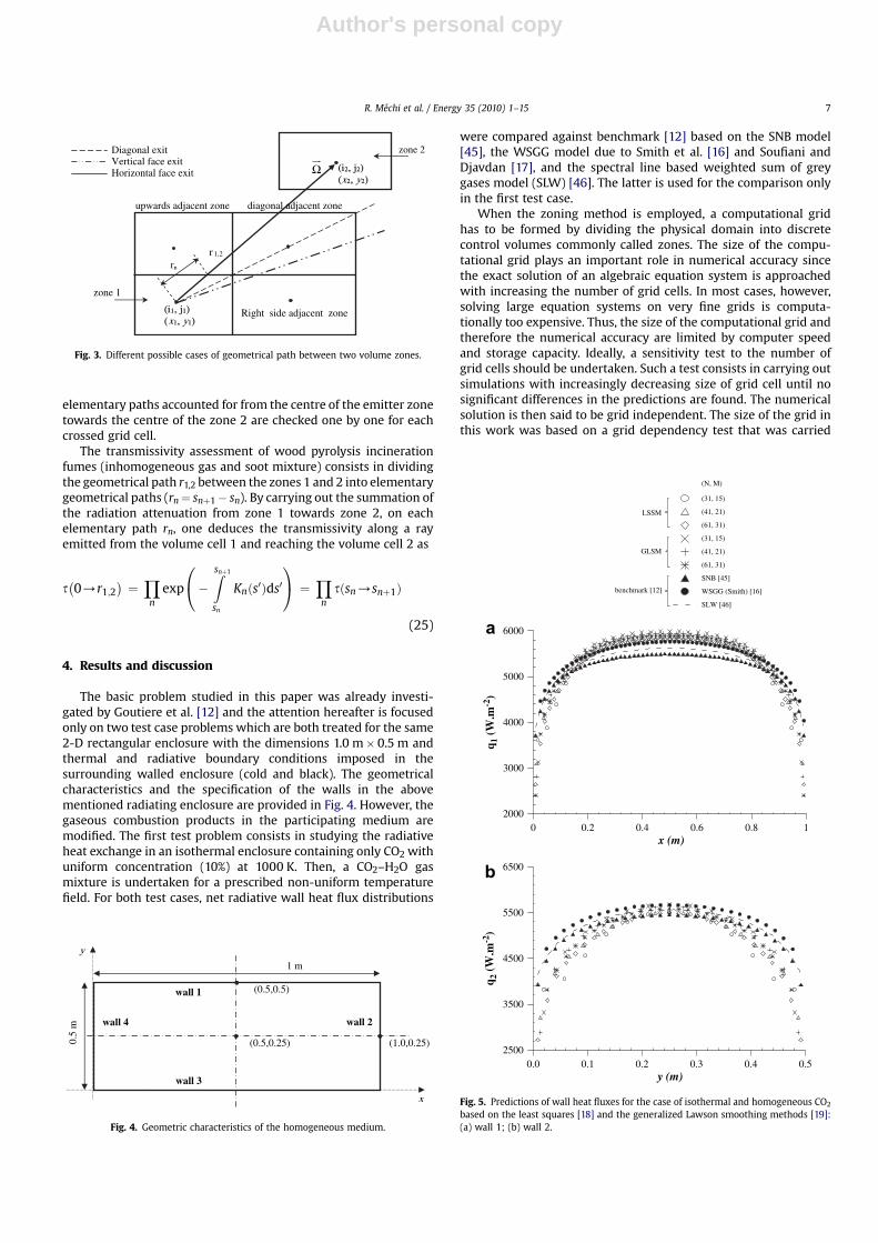
To calculate the DEAs between a pair of finite volume zonesaffected of numbers 1 and 2, a numerical method is developed fordetection of the entry and exit of a volume zone n located on thepath of an emitted amount of radiation by the zone 1 and directlyintercepted by the zone 2. Fig. 3 illustrates the case of radiativeexchange between an arbitrary pair of volume zones. The emitterone indicated by ‘‘zone 1’’ is surrounded by three neighbouredzones situated at the right, the top and the diagonal positions. The

mn

Discretized surface zone

rmn

One surface element subdivision

dAm

dAn

mn

nn

Fig. 1. Direct numerical integration technique: case of two surface zones [31].

),( ξηΩ

J

J+1

I+1

M(x, y)

x

y

44 33

2211

⎪⎪⎩

⎪⎪⎨

⎧

=

=

v

u

y(J+1) − y(J)

y − y(J)x(I+1) − x(I)

x − x(I)

I

s

sn(xn, yn)

O

sn+1 (xn+1 ,yn+1 )

Fig. 2. Definition of the bilinear interpolation of the global absorption coefficient ofa gas–soot mixture at a point M [43,44].



elementary paths accounted for from the centre of the emitter zonetowards the centre of the zone 2 are checked one by one for eachcrossed grid cell.

The transmissivity assessment of wood pyrolysis incinerationfumes (inhomogeneous gas and soot mixture) consists in dividingthe geometrical path r1,2 between the zones 1 and 2 into elementarygeometrical paths (rn¼ snþ1� sn). By carrying out the summation ofthe radiation attenuation from zone 1 towards zone 2, on eachelementary path rn, one deduces the transmissivity along a rayemitted from the volume cell 1 and reaching the volume cell 2 as

s�0/r1;2

�¼Y

nexp

0@�

Zsnþ1

sn

Knðs0Þds0

1A ¼ Y

nsðsn/snþ1Þ

(25)

4. Results and discussion

The basic problem studied in this paper was already investi-gated by Goutiere et al. [12] and the attention hereafter is focusedonly on two test case problems which are both treated for the same2-D rectangular enclosure with the dimensions 1.0 m� 0.5 m andthermal and radiative boundary conditions imposed in thesurrounding walled enclosure (cold and black). The geometricalcharacteristics and the specification of the walls in the abovementioned radiating enclosure are provided in Fig. 4. However, thegaseous combustion products in the participating medium aremodified. The first test problem consists in studying the radiativeheat exchange in an isothermal enclosure containing only CO2 withuniform concentration (10%) at 1000 K. Then, a CO2–H2O gasmixture is undertaken for a prescribed non-uniform temperaturefield. For both test cases, net radiative wall heat flux distributions

were compared against benchmark [12] based on the SNB model[45], the WSGG model due to Smith et al. [16] and Soufiani andDjavdan [17], and the spectral line based weighted sum of greygases model (SLW) [46]. The latter is used for the comparison onlyin the first test case.

When the zoning method is employed, a computational gridhas to be formed by dividing the physical domain into discretecontrol volumes commonly called zones. The size of the compu-tational grid plays an important role in numerical accuracy sincethe exact solution of an algebraic equation system is approachedwith increasing the number of grid cells. In most cases, however,solving large equation systems on very fine grids is computa-tionally too expensive. Thus, the size of the computational grid andtherefore the numerical accuracy are limited by computer speedand storage capacity. Ideally, a sensitivity test to the number ofgrid cells should be undertaken. Such a test consists in carrying outsimulations with increasingly decreasing size of grid cell until nosignificant differences in the predictions are found. The numericalsolution is then said to be grid independent. The size of the grid inthis work was based on a grid dependency test that was carried

zone 2

zone 1

Diagonal exit Vertical face exit Horizontal face exit

r 1,2

rn

(i1, j1)(x1, y1)

(i2, j2)(x2, y2)

upwards adjacent zone

Right side adjacent zone

Ω

diagonal adjacent zone

Fig. 3. Different possible cases of geometrical path between two volume zones.

1 m

(0.5,0.5)

(0.5,0.25) (1.0,0.25)

wall 1

wall 2

wall 3

wall 4

x

y

0.5

m

Fig. 4. Geometric characteristics of the homogeneous medium.

0 0.2 0.4 0.6 0.8 1x (m)

2000

3000

4000

5000

6000

LSSM

GLSM

benchmark [12]

(N, M)

(31, 15)

(41, 21)

(61, 31)

(31, 15)

(41, 21)

(61, 31)

SNB [45]

WSGG (Smith) [16]

SLW [46]

0.0 0.1 0.2 0.3 0.4 0.5y (m)

2500

3500

4500

5500

6500

q 2 (

W.m

-2)

q 1 (

W.m

-2)

a

b

Fig. 5. Predictions of wall heat fluxes for the case of isothermal and homogeneous CO2

based on the least squares [18] and the generalized Lawson smoothing methods [19]:(a) wall 1; (b) wall 2.



out by Goutiere et al. [12] for the two-dimensional rectangularfurnace (Fig. 4).

4.1. Case of homogeneous media

4.1.1. First test caseThe CO2 concentration is supposed to be uniform in all the

rectangular enclosure where the partial pressure is 0.1 atm (firsttest case in [12]). The WSGG model parameters evaluated fromFarag [15] are incorporated into the developed 2-D computationalcode.

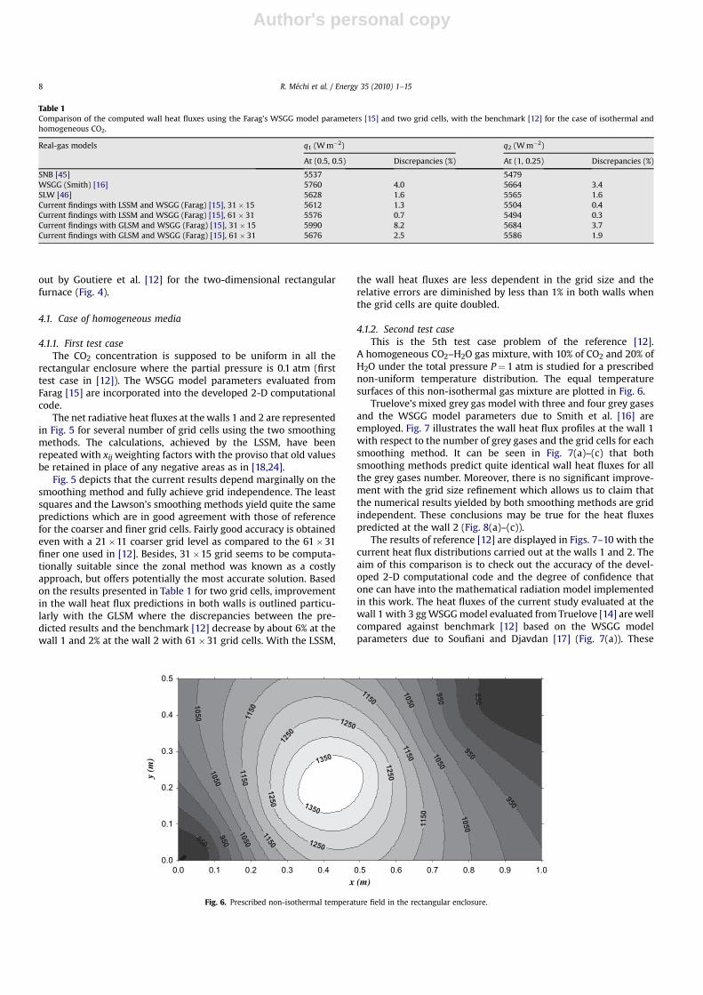
The net radiative heat fluxes at the walls 1 and 2 are representedin Fig. 5 for several number of grid cells using the two smoothingmethods. The calculations, achieved by the LSSM, have beenrepeated with xij weighting factors with the proviso that old valuesbe retained in place of any negative areas as in [18,24].

Fig. 5 depicts that the current results depend marginally on thesmoothing method and fully achieve grid independence. The leastsquares and the Lawson’s smoothing methods yield quite the samepredictions which are in good agreement with those of referencefor the coarser and finer grid cells. Fairly good accuracy is obtainedeven with a 21�11 coarser grid level as compared to the 61�31finer one used in [12]. Besides, 31�15 grid seems to be computa-tionally suitable since the zonal method was known as a costlyapproach, but offers potentially the most accurate solution. Basedon the results presented in Table 1 for two grid cells, improvementin the wall heat flux predictions in both walls is outlined particu-larly with the GLSM where the discrepancies between the pre-dicted results and the benchmark [12] decrease by about 6% at thewall 1 and 2% at the wall 2 with 61�31 grid cells. With the LSSM,

the wall heat fluxes are less dependent in the grid size and therelative errors are diminished by less than 1% in both walls whenthe grid cells are quite doubled.

4.1.2. Second test caseThis is the 5th test case problem of the reference [12].

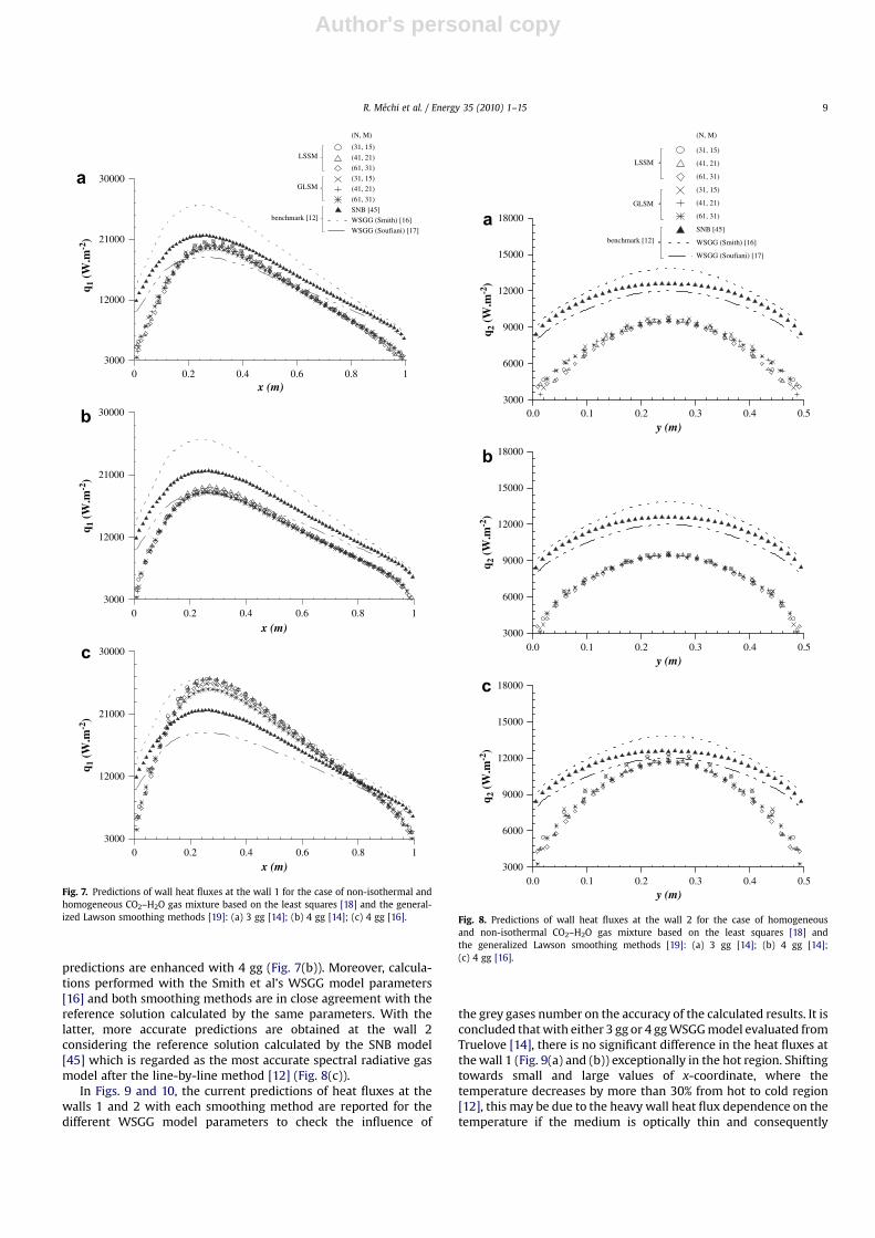
A homogeneous CO2–H2O gas mixture, with 10% of CO2 and 20% ofH2O under the total pressure P¼ 1 atm is studied for a prescribednon-uniform temperature distribution. The equal temperaturesurfaces of this non-isothermal gas mixture are plotted in Fig. 6.

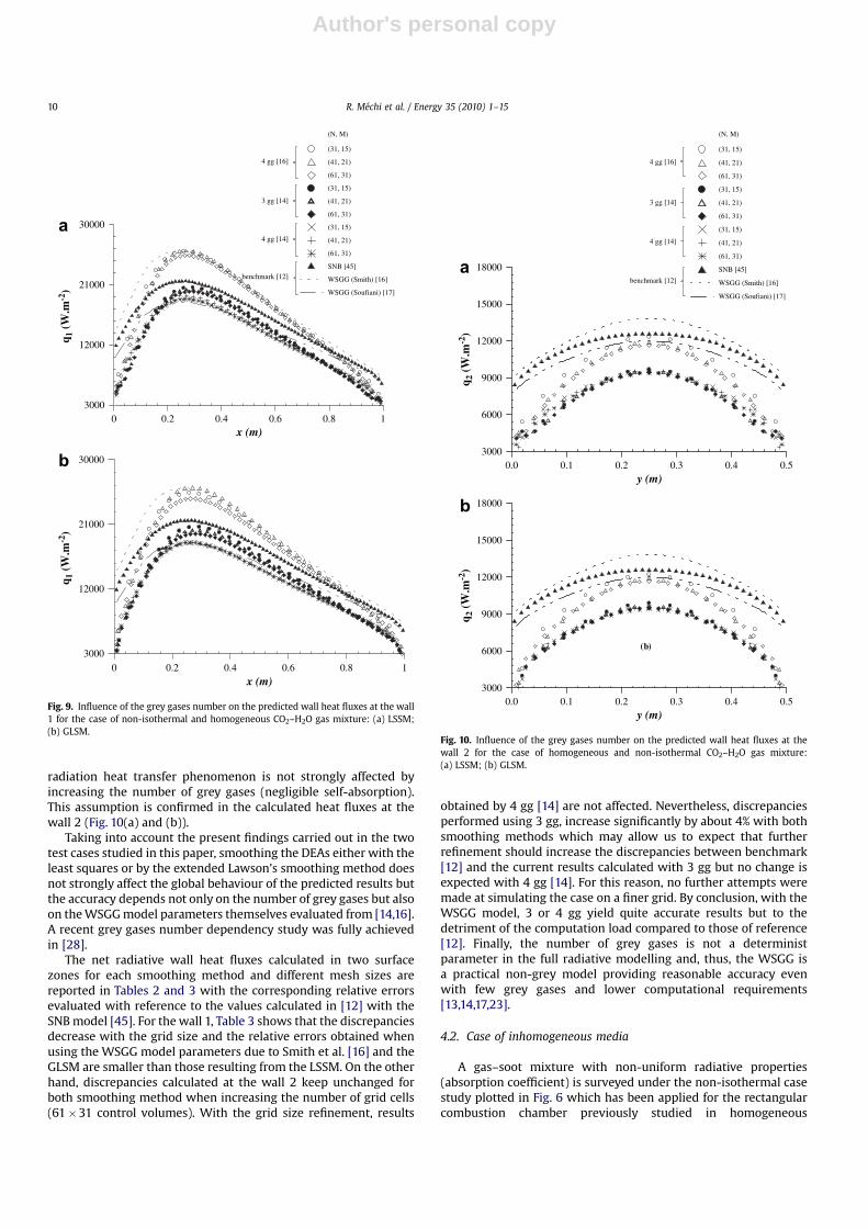
Truelove’s mixed grey gas model with three and four grey gasesand the WSGG model parameters due to Smith et al. [16] areemployed. Fig. 7 illustrates the wall heat flux profiles at the wall 1with respect to the number of grey gases and the grid cells for eachsmoothing method. It can be seen in Fig. 7(a)–(c) that bothsmoothing methods predict quite identical wall heat fluxes for allthe grey gases number. Moreover, there is no significant improve-ment with the grid size refinement which allows us to claim thatthe numerical results yielded by both smoothing methods are gridindependent. These conclusions may be true for the heat fluxespredicted at the wall 2 (Fig. 8(a)–(c)).

The results of reference [12] are displayed in Figs. 7–10 with thecurrent heat flux distributions carried out at the walls 1 and 2. Theaim of this comparison is to check out the accuracy of the devel-oped 2-D computational code and the degree of confidence thatone can have into the mathematical radiation model implementedin this work. The heat fluxes of the current study evaluated at thewall 1 with 3 gg WSGG model evaluated from Truelove [14] are wellcompared against benchmark [12] based on the WSGG modelparameters due to Soufiani and Djavdan [17] (Fig. 7(a)). These

Table 1Comparison of the computed wall heat fluxes using the Farag’s WSGG model parameters [15] and two grid cells, with the benchmark [12] for the case of isothermal andhomogeneous CO2.

Real-gas models q1 (W m�2) q2 (W m�2)

At (0.5, 0.5) Discrepancies (%) At (1, 0.25) Discrepancies (%)

SNB [45] 5537 5479WSGG (Smith) [16] 5760 4.0 5664 3.4SLW [46] 5628 1.6 5565 1.6Current findings with LSSM and WSGG (Farag) [15], 31� 15 5612 1.3 5504 0.4Current findings with LSSM and WSGG (Farag) [15], 61� 31 5576 0.7 5494 0.3Current findings with GLSM and WSGG (Farag) [15], 31� 15 5990 8.2 5684 3.7Current findings with GLSM and WSGG (Farag) [15], 61� 31 5676 2.5 5586 1.9

0.0 0.1 0.2 0.3 0.4 0.5 0.6 0.7 0.8 0.9 1.0x (m)

0.0

0.1

0.2

0.3

0.4

0.5

y (m

)

Fig. 6. Prescribed non-isothermal temperature field in the rectangular enclosure.



predictions are enhanced with 4 gg (Fig. 7(b)). Moreover, calcula-tions performed with the Smith et al’s WSGG model parameters[16] and both smoothing methods are in close agreement with thereference solution calculated by the same parameters. With thelatter, more accurate predictions are obtained at the wall 2considering the reference solution calculated by the SNB model[45] which is regarded as the most accurate spectral radiative gasmodel after the line-by-line method [12] (Fig. 8(c)).

In Figs. 9 and 10, the current predictions of heat fluxes at thewalls 1 and 2 with each smoothing method are reported for thedifferent WSGG model parameters to check the influence of

the grey gases number on the accuracy of the calculated results. It isconcluded that with either 3 gg or 4 gg WSGG model evaluated fromTruelove [14], there is no significant difference in the heat fluxes atthe wall 1 (Fig. 9(a) and (b)) exceptionally in the hot region. Shiftingtowards small and large values of x-coordinate, where thetemperature decreases by more than 30% from hot to cold region[12], this may be due to the heavy wall heat flux dependence on thetemperature if the medium is optically thin and consequently

0 0.2 0.4 0.6 0.8 1x (m)

x (m)

x (m)

3000

12000

21000

30000

LSSM

GLSM

benchmark [12]

(N, M)

(31, 15)

(41, 21)

(61, 31)

(31, 15)

(41, 21)

(61, 31)

SNB [45]

WSGG (Smith) [16]

WSGG (Soufiani) [17]

0 0.2 0.4 0.6 0.8 13000

12000

21000

30000

0 0.2 0.4 0.6 0.8 13000

12000

21000

30000

q 1 (

W.m

-2)

q 1 (

W.m

-2)

q 1 (

W.m

-2)

a

b

c

Fig. 7. Predictions of wall heat fluxes at the wall 1 for the case of non-isothermal andhomogeneous CO2–H2O gas mixture based on the least squares [18] and the general-ized Lawson smoothing methods [19]: (a) 3 gg [14]; (b) 4 gg [14]; (c) 4 gg [16].

0.0 0.1 0.2 0.3 0.4 0.5y (m)

3000

6000

9000

12000

15000

18000

(N, M)

(31, 15)

(41, 21)

(61, 31)

(31, 15)

(41, 21)

(61, 31)

SNB [45]

WSGG (Smith) [16]


benchmark [12]

LSSM

GLSM

q 2 (

W.m

-2)

0.0 0.1 0.2 0.3 0.4 0.5y (m)

3000

6000

9000

12000

15000

18000

q 2 (

W.m

-2)

0.0 0.1 0.2 0.3 0.4 0.5y (m)

3000

6000

9000

12000

15000

18000

q 2 (

W.m

-2)

a

b

c

Fig. 8. Predictions of wall heat fluxes at the wall 2 for the case of homogeneousand non-isothermal CO2–H2O gas mixture based on the least squares [18] andthe generalized Lawson smoothing methods [19]: (a) 3 gg [14]; (b) 4 gg [14];(c) 4 gg [16].



radiation heat transfer phenomenon is not strongly affected byincreasing the number of grey gases (negligible self-absorption).This assumption is confirmed in the calculated heat fluxes at thewall 2 (Fig. 10(a) and (b)).

Taking into account the present findings carried out in the twotest cases studied in this paper, smoothing the DEAs either with theleast squares or by the extended Lawson’s smoothing method doesnot strongly affect the global behaviour of the predicted results butthe accuracy depends not only on the number of grey gases but alsoon the WSGG model parameters themselves evaluated from [14,16].A recent grey gases number dependency study was fully achievedin [28].

The net radiative wall heat fluxes calculated in two surfacezones for each smoothing method and different mesh sizes arereported in Tables 2 and 3 with the corresponding relative errorsevaluated with reference to the values calculated in [12] with theSNB model [45]. For the wall 1, Table 3 shows that the discrepanciesdecrease with the grid size and the relative errors obtained whenusing the WSGG model parameters due to Smith et al. [16] and theGLSM are smaller than those resulting from the LSSM. On the otherhand, discrepancies calculated at the wall 2 keep unchanged forboth smoothing method when increasing the number of grid cells(61�31 control volumes). With the grid size refinement, results

obtained by 4 gg [14] are not affected. Nevertheless, discrepanciesperformed using 3 gg, increase significantly by about 4% with bothsmoothing methods which may allow us to expect that furtherrefinement should increase the discrepancies between benchmark[12] and the current results calculated with 3 gg but no change isexpected with 4 gg [14]. For this reason, no further attempts weremade at simulating the case on a finer grid. By conclusion, with theWSGG model, 3 or 4 gg yield quite accurate results but to thedetriment of the computation load compared to those of reference[12]. Finally, the number of grey gases is not a deterministparameter in the full radiative modelling and, thus, the WSGG isa practical non-grey model providing reasonable accuracy evenwith few grey gases and lower computational requirements[13,14,17,23].

4.2. Case of inhomogeneous media

A gas–soot mixture with non-uniform radiative properties(absorption coefficient) is surveyed under the non-isothermal casestudy plotted in Fig. 6 which has been applied for the rectangularcombustion chamber previously studied in homogeneous

0 0.2 0.4 0.6 0.8 1x (m)

0 0.2 0.4 0.6 0.8 1x (m)

3000

12000

21000

30000

3000

12000

21000

30000

a

b

(N, M)

(31, 15)

(41, 21)

(61, 31)

(31, 15)

(41, 21)

(61, 31)

(31, 15)

(41, 21)

(61, 31)

SNB [45]

WSGG (Smith) [16]


4 gg [16]

3 gg [14]

4 gg [14]

benchmark [12]

q 1 (

W.m

-2)

q 1 (

W.m

-2)

Fig. 9. Influence of the grey gases number on the predicted wall heat fluxes at the wall1 for the case of non-isothermal and homogeneous CO2–H2O gas mixture: (a) LSSM;(b) GLSM.

0.0 0.1 0.2 0.3 0.4 0.5y (m)

3000

6000

9000

12000

15000

18000benchmark [12]

4 gg [16]

3 gg [14]

a

b

(N, M)

(31, 15)

(41, 21)

(61, 31)

(31, 15)

(41, 21)

(61, 31)

(31, 15)

(41, 21)

(61, 31)

SNB [45]

WSGG (Smith) [16]


4 gg [14]

(b)

q 2 (

W.m

-2)

0.0 0.1 0.2 0.3 0.4 0.5y (m)

3000

6000

9000

12000

15000

18000

q 2 (

W.m

-2)

Fig. 10. Influence of the grey gases number on the predicted wall heat fluxes at thewall 2 for the case of homogeneous and non-isothermal CO2–H2O gas mixture:(a) LSSM; (b) GLSM.



conditions. The DEAs are carried out by using two temperature-dependent absorption coefficient models of the gas–soot mixture,taking into account the dependence on temperature of the local gascomposition at each volume zone and, thus, of all the inhomoge-neous paths in the medium. In this section, the radiation model(WSGG model together with the zone method) will be extended topredict the net radiative wall heat fluxes at walls 1 and 2 of therectangular combustion chamber (Fig. 4). The numerical procedurefor the detection of entry and exit of the ray emitted from onevolume zone to another one at crossed volume zones in such raydirection is applied in conjunction with the technique of bilinearinterpolation.

In this paper, the inhomogeneous aspect of the semi-trans-parent medium (gas–soot mixture) is undertaken by using twocomponents’ absorption coefficient; one for the soot particlesand another for the gas mixture. This approach was suggestedby many authors among them one can refer to Johnson andBeer [23], Truelove [14] and Murty et al. [47]. Truelove chosea temperature-independent specific absorption coefficient kg ofthe gas mixture and one order polynomial function intemperature for the specific absorption coefficient ks of the soot(thermal equilibrium is assumed). Thus, for a gas–soot mixture,we obtain

Kgas�soot ¼ Kg þ Ks ¼ kg�PCO2

þ PH2O�þ ksðTÞC (26)

where

ksðTÞ ¼ b1½1þ bT ðT � 2000Þ� (27)

with b1¼1232.4 m2 kg�1 and bT z 4.8� 10�4 K�1.Murty et al. [47] have proposed one grey gas to deal with

non-grey semi-transparent gas–soot mixture. This may allow theevaluation of the DEAs with reasonable computational require-ments since the DFAs are not only equal to the TEAs but also

to the DEAs (black-walled enclosure). The specific absorptioncoefficients (kg and ks) are expressed by two polynomials intemperature as

Kgas�soot ¼ kgðTÞ�PCO2

þ PH2O�þ ksðTÞC (28)

where

8>>><>>>:

kgðTÞ ¼X5

n¼1

fg;nTn�1

ksðTÞ ¼X3

n¼1

fs;nTn�1

(29)

The constants fg,n and fs,n are obtained from [47].Hereafter, the effect of the number of grey gases on the

numerical predictions will be checked by using one grey gasabsorption coefficient model due to Murty et al. [47] and that ofTruelove [14] with several grey gases (3 and 4 gg).

The net radiative wall heat flux distributions at the walls 1 and 2of the rectangular enclosure (Fig. 4), for the inhomogeneous CO2–H2O–soot mixture, are represented in Figs. 11–13 and 12–14respectively. The same behaviour is obtained using the least squaresand the Lawson’s smoothing methods for all number of grid cellsand the calculated heat fluxes can be considered as grid indepen-dent. The mesh refinement did not affect sensitively the computedfluxes and satisfactory results can be reached with relatively smallnumber of grids and the discrepancies at this level are lower in theinhomogeneous case by comparison to the homogeneous one. Infact, with 31�15 and 41�21 control volumes, we attain perhapsthe same findings and no significant change is expected whenincreasing enough the grid size (Figs. 11(a), (b) and 12(a)–(c)).

The same test problem is studied by introducing the parametersof Murty et al. [47]. Tests have shown an over-estimation of theresults based on these parameters as compared to those obtainedwith several grey gases based on the parameters of Truelove [14].With the Murty et al’s model [47], the tendencies of the two

Table 2Comparison of the computed wall heat fluxes using the Truelove’s WSGG model parameters (3 gg and 4 gg) [14] and the Smith et al’s parameters [16] with 31�15 grid cells,with benchmark [12] for the case of non-isothermal and homogeneous CO2–H2O gas mixture.



SNB [45] 21,630 12,668WSGG (Smith) [16] 26,030 20.3 13,868 9.5WSGG (Soufiani) [17] 18,330 �15.3 11,936 �5.8Current findings with LSSM and WSGG (Truelove) [14], 3 gg 20,377 �5.8 9694 �23.4Current findings with LSSM and WSGG (Truelove) [14], 4 gg 18,758 �13.2 9581 �24.3Current findings with LSSM and WSGG (Smith) [16], 4 gg 25,920 19.8 12,333 �2.6Current findings with GLSM and WSGG (Truelove) [14], 3 gg 20,456 �5.4 9891 �21.9Current findings with GLSM and WSGG (Truelove) [14], 4 gg 18,418 �14.8 9556 �24.5Current findings with GLSM and WSGG (Smith) [16], 4 gg 25,306 16.9 12,229 �3.4

Table 3Comparison of the computed wall heat fluxes using the Truelove’s WSGG model parameters (3 gg and 4 gg) [14] and the Smith et al’s parameters [16] with 61�31 grid cells,with benchmark [14] for the case of non-isothermal and homogeneous CO2–H2O gas mixture.



SNB [45] 21,630 12,668WSGG (Smith) [16] 26,030 20.3 13,868 9.5WSGG (Soufiani) [17] 18,330 �15.3 11,936 �5.8Current findings with LSSM and WSGG (Truelove) [14], 3 gg 19,779 �8.5 9433 �23.4Current findings with LSSM and WSGG (Truelove) [14], 4 gg 18,818 �13.0 9404 �24.3Current findings with LSSM and WSGG (Smith) [16], 4 gg 25,313 17.0 11,667 �7.9Current findings with GLSM and WSGG (Truelove) [14], 3 gg 19,520 �9.7 9505 �24.9Current findings with GLSM and WSGG (Truelove) [14], 4 gg 18,421 �14.8 9401 �25.7Current findings with GLSM and WSGG (Smith) [16], 4 gg 24,512 13.3 11,666 �7.9



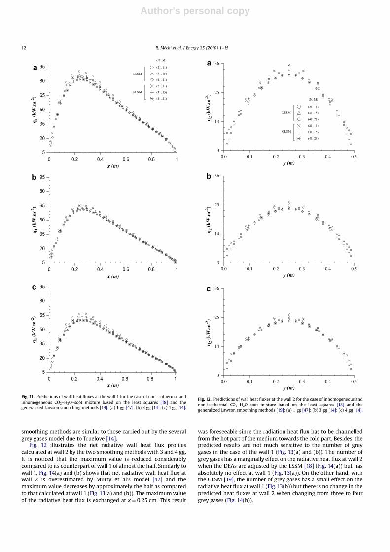
smoothing methods are similar to those carried out by the severalgrey gases model due to Truelove [14].

Fig. 12 illustrates the net radiative wall heat flux profilescalculated at wall 2 by the two smoothing methods with 3 and 4 gg.It is noticed that the maximum value is reduced considerablycompared to its counterpart of wall 1 of almost the half. Similarly towall 1, Fig. 14(a) and (b) shows that net radiative wall heat flux atwall 2 is overestimated by Murty et al’s model [47] and themaximum value decreases by approximately the half as comparedto that calculated at wall 1 (Fig. 13(a) and (b)). The maximum valueof the radiative heat flux is exchanged at x¼ 0.25 cm. This result

was foreseeable since the radiation heat flux has to be channelledfrom the hot part of the medium towards the cold part. Besides, thepredicted results are not much sensitive to the number of greygases in the case of the wall 1 (Fig. 13(a) and (b)). The number ofgrey gases has a marginally effect on the radiative heat flux at wall 2when the DEAs are adjusted by the LSSM [18] (Fig. 14(a)) but hasabsolutely no effect at wall 1 (Fig. 13(a)). On the other hand, withthe GLSM [19], the number of grey gases has a small effect on theradiative heat flux at wall 1 (Fig. 13(b)) but there is no change in thepredicted heat fluxes at wall 2 when changing from three to fourgrey gases (Fig. 14(b)).

0 0.2 0.4 0.6 0.8 1x (m)

5

20

35

50

65

80

95 (N , M)

(21, 11)

(31, 15)

(41, 21)

(21, 11)

(31, 15)

(41, 21)

LSSM

GLSM

a

b

c

q 1 (

kW.m

-2)

0 0.2 0.4 0.6 0.8 1x (m)

5

20

35

50

65

80

95

q 1 (

kW.m

-2)

0 0.2 0.4 0.6 0.8 1x (m)

5

20

35

50

65

80

95

q 1 (

kW.m

-2)

Fig. 11. Predictions of wall heat fluxes at the wall 1 for the case of non-isothermal andinhomogeneous CO2–H2O–soot mixture based on the least squares [18] and thegeneralized Lawson smoothing methods [19]: (a) 1 gg [47]; (b) 3 gg [14]; (c) 4 gg [14].

0.0y (m)

3

14

25

36

(N, M)

(21, 11)

(31, 15)

(41, 21)

(21, 11)

(31, 15)

(41, 21)

LSSM

GLSM

3

14

25

36

3

14

25

36

q 2 (

kW.m

-2)

q 2 (

kW.m

-2)

q 2 (

kW.m

-2)

0.1 0.2 0.3 0.50.4

0.0y (m)

0.1 0.2 0.3 0.50.4

0.0y (m)

0.1 0.2 0.3 0.50.4

a

b

c

Fig. 12. Predictions of wall heat fluxes at the wall 2 for the case of inhomogeneous andnon-isothermal CO2–H2O–soot mixture based on the least squares [18] and thegeneralized Lawson smoothing methods [19]: (a) 1 gg [47]; (b) 3 gg [14]; (c) 4 gg [14].



According to Figs. 11–14, the grid refinement does not result ina significant improvement of the predicted radiative wall heatfluxes with all the WSGG model parameters [14,47] and with bothsmoothing methods. This result is of a great interest since it makesit possible to reduce the memory size allocated for the matriceswithout too much influence on the results, alleviating thus theprohibitive computing times. The results predicted with bothsmoothing methods show that the presence of soot even witha weak concentration (10�3 kg m�3) assigns considerably the netradiative wall heat fluxes, which is in concordance with the liter-ature [22,26,27,48,49]. Therefore, the presence of soot accentuatesthe radiative transfers towards the walls and thus decreases thetemperature in the medium (temperature of the luminous flame)due to the continuous heating of the walls by radiative exchangebetween the gas species and the soot particles on one hand, and theenclosing walls on the other side.

The discrepancies between model predictions and bench-mark results arise, inter alia, because the surface temperatures,or so-called irradiation temperatures Ts in all calculation casesare set at 0 K, while the WSGG model used here [14,16] isdesigned and is good for region 600< Ts < 2400 K. Irradiationtemperature Ts plays important role for the evaluation of totalgas absorptivity and, thus, the wall heat fluxes, particularly inthe case of CO2–H2O gas mixture due to the large absorptionbands of H2O [7,16]. This shortcoming of the WSGG model was

also outlined by Soufiani and Djavdan [17] and more recentlyby Trivic [28].

5. Conclusions

Two smoothing methods of the DEAs have been presented andguessed within a computer code allowing radiative calculationsin 2-D black-walled rectangular enclosure and the currentnumerical predictions for two homogeneous test cases have beenassessed against benchmark solutions. In a second time, theproposed radiation model based on the zonal method of Hottel inconjunction with the most attractive WSGG model parametershas been extended to inhomogeneous semi-transparent medium.For this reason, temperature-dependent absorption coefficients ofgas–soot mixture were used, taking into account the spatialdependence of the radiative properties of the semi-transparentmedium. With the results of the present study based on theradiative pattern mentioned above, the following conclusions arereached:

(1) The predicted wall radiative heat fluxes are fairly wellcompared against benchmark [12], calculated by the SNBmodel [45], in two homogeneous test cases respectively with

5

20

35

50

65

80

951 gg [47]

3 gg [14]

4 gg [14]

(N, M)

(21, 11)

(31, 15)

(41, 21)

(21, 11)

(31, 15)

(41, 21)

(21, 11)

(31, 15)

(41, 21)

0

x (m)

5

20

35

50

65

80

95

0.2 0.4 0.6 0.8 1

0

x (m)0.2 0.4 0.6 0.8 1

q 1 (

kW.m

-2)

q 1 (

kW.m

-2)

a

b

Fig. 13. Influence of the grey gases number on the predicted wall heat fluxes at thewall 1 for the case of non-isothermal and inhomogeneous CO2–H2O–soot mixture: (a)LSSM; (b) GLSM.

3

14

25

36

(N, M)

(21, 11)

(31, 15)

(41, 21)

(21, 11)

(31, 15)

(41, 21)

(21, 11)

(31, 15)

(41, 21)

3 gg [14]

4 gg [14]

1 gg [47]

0.0

y (m)

3

14

25

36

0.50.40.30.20.1

0.0

y (m)0.50.40.30.20.1

q 2 (

kW.m

-2)

q 2 (

kW.m

-2)

b

a

Fig. 14. Influence of the grey gases number on the predicted wall heat fluxes at thewall 2 for the case of inhomogeneous and non-isothermal CO2–H2O–soot mixture:(a) LSSM; (b) GLSM.



isothermal and single participating gas CO2 and then with non-isothermal CO2–H2O gas mixture. Although the LSSM givessatisfactory results as shown in the comparisons done all theway through this paper, this smoothing method has a majordrawback namely the negativity of some adjusted DEA esti-mates as pointed out by Larsen and Howell [18]. Thisproblem has been withdrawn here by taking the old values(raw data) in place of any negative areas. Also, the techniqueof reset to zero of the negative adjusted values during thesmoothing iterative process may be well used solution inseveral similar cases. Besides, with the GLSM, the abovementioned problem is far away (no negative values arereturned with this algorithm). Even so, the marginaldiscrepancies between the results of both smoothingmethods may arise from the numerical errors of eachsmoothing procedure which will lead to different adjustedDEAs initially not accurately estimated (direct numericalintegration). Since the initial estimates are evaluatednumerically, this will result in considerable duration of thecomputation of these areas and, thus, in an uncontrollableloss of accuracy [50]. Moreover, as the exact nature of thedeficiencies in the raw exchange area data is often notknown, particularly for the large equation systems, someindividual areas may move away from their true values afteradjustment as it was intended in [18] and confirmed later in[24]. Furthermore, it was demonstrated that the improve-ment in the wall heat fluxes did not occur when using theLSSM unless particular boundary conditions have to beconsidered [18], explaining so the good agreement reached inthe first isothermal test case (cold walls and isothermalmedium) and the discrepancies, outlined in the secondhomogeneous test case, between the least squares’ currentresults and those provided in [12].

(2) The non-greyness nature of the considered real species withuniform and non-uniform radiative properties which may beencountered in the most industrial combustor systems (CO2,CO2–H2O gas mixture, CO2–H2O–soot mixture) operating athigh temperature has been seriously investigated by usingseveral WSGG model parameters [14–16]. This should bea good standard against which the efficiency of thecomputer code can be checked and hence the accuracy ofthe Hottel’s zonal method even when it is associated withless accurate radiative properties models compared to theexcessive computationally spectral methods (SLW, SNB, SNB-CK, .).

(3) The mathematical model equations presented in the case ofinhomogeneous media based on the bilinear interpolation ofthe absorption coefficient of the participating media are easy toimplement in any computer code for the calculations of radi-ative heat transfer, providing fully grid independent solutionswith lower computational cost. The general concept of thatmodel joins simultaneously the advancements of both thediscrete transfer method and those of the conventional zonalmethod allowing the extension of the latter to inhomogeneoussemi-transparent media.

(4) The new mathematical radiation model and the numericalcode developed in this paper enable radiative transfer calcu-lations with quite reasonable accuracy which greatly dependson the accuracy of the gas radiative properties. Therefore, it isexpected that the present results can be perfected whenadopting more accurate non-grey gas models such as the SLW[51] which has been recently applied to non-isothermal andnon-homogeneous gas mixtures in multi-dimensional enclo-sures [49] as an efficient and accurate alternative to theconventional WSGG model due to Hottel.

References

[1] Yuen WW, Takara EE. Development of a generalized zonal method for analysisof radiative transfer in absorbing and anisotropically scattering media. NumerHeat Transf B 1994;25(1):75–96.

[2] Yuen WW. The multiple absorption coefficient zonal method (MACZM), anefficient computational approach for the analysis of radiative heat transfer inmultidimensional inhomogeneous nongrey media. Numer Heat Transf B2006;49(2):89–103.

[3] Khan YU, Lawson DA, Tucker RJ. Banded radiative heat transfer analysis.Commun Numer Methods Eng 1997;13(10):803–13.

[4] Goyhenehe JM, Sacadura JF. The zone method: a new explicit matrix relation tocalculate the total exchange areas in anisotropically scattering medium boundedby anisotropically reflecting walls. ASME J Heat Transf 2002;124(4):696–703.

[5] Hottel HC, Cohen ES. Radiant heat exchange in a gas-filled enclosure: allow-ance for non-uniformity of gas temperature. AIChE J 1958;4(1):3–14.

[6] Hottel HC, Sarofim AF. Radiative transfer. New York: McGraw-Hill; 1967.[7] Ben Nejma F, Mazgar A, Abadallah N, Charrada K. Entropy generation through

combined non-grey gas radiation and forced convection between two parallelplates. Energy 2008;33(7):1169–78.

[8] Bejan A, Dan N, Cacuci DG, Schutz W. On the thermodynamic efficiency ofenergy conversion during the expansion of a mixture of hot particles, steamand liquid water. Energy 1997;22(12):1119–33.

[9] Modak AT. Radiation from products of combustion. Fire Saf J 1979;1(6):339–61.

[10] Leckner B. Spectral and total emissivity of water vapor and carbon dioxide.Combust Flame 1972;19(1):33–48.

[11] Grosshandler WL, Modak AT. Radiation from nonhomogeneous combustionproducts. In: Proceedings of the eighteenth symposium (international) oncombustion. Pittsburgh, PA: The Combustion Institute; 1981. p. 601–9.

[12] Goutiere V, Liu F, Charette A. An assessment of real-gas modelling in 2Denclosures. J Quant Spectrosc Radiat Transf 2000;64(3):299–326.

[13] Coelho PJ. Numerical simulation of radiative heat transfer from non-grey gasesin three dimensional enclosures. J Quant Spectrosc Radiat Transf 2002;74(3):307–28.

[14] Truelove JS. A mixed grey gas model for flame radiation. Report AERE-R-8494.United Kingdom Atomic Energy Authority Harwell; 1976.

[15] Farag IH. Non-luminous gas radiation: approximate emissivity models (A83-42663 20-34). In: Munich, West GermanyProceedings of the seventh heattransfer (international) conference, vol. 2. Washington: DC: HemispherePublishing Corp.; 1982. p. 487–92.

[16] Smith FT, Shen ZF, Friedman JN. Evaluation of coefficients for the weightedsum of grey gases model. J Heat Transf 1982;104(4):602–8.

[17] Soufiani A, Djavdan EA. Comparison between weighted-sum-of-grey-gasesand statistical narrow-band models for combustion applications. CombustFlame 1994;97(2):240–50.

[18] Larsen ME, Howell JR. Least-squares smoothing of direct exchange areas inzonal analysis. J Heat Transf 1986;108(1):239–42.

[19] Lawson DA. An improved method for smoothing approximate exchange areas.Int J Heat Mass Transf 1995;38(16):3109–10.

[20] Leersum JV. A method for determining a consistent set of radiation view factorfrom a set generated by a nonexact method. Int J Heat Fluid Flow1989;10(1):83–5.

[21] Noble JJ. The zone method: explicit matrix relations for total exchange areas.Int J Heat Mass Transf 1975;108(2):261–9.

[22] Liu F, Becker HA, Bindar YA. Comparative study of radiative heat transfermodelling in gas-fired furnaces using the simple grey gas and theweighted-sum-of-grey-gases models. Int J Heat Mass Transf 1998;41(22):3357–71.

[23] Johnson TR, Beer JM. Radiative heat transfer in furnaces: further developmentof the zone method of analysis. In: Proceedings of the fourteenth symposium(international) on combustion. Pennsylvania, USA: The Combustion Institute;1973. p. 639–49.

[24] Murty CVS, Murty BSN. Significance of exchange area adjustment in zonemodelling. Int J Heat Mass Transf 1991;34(2):499–503.

[25] Khan YU, Lawson DA, Tucker RJ. Simple models of spectral radiative propertiesof carbon dioxide. Int J Heat Mass Transf 1997;40(15):3581–93.

[26] Bressloff NW. The influence of soot loading on weighted sum of grey gasessolutions to the radiative transfer equation across mixtures of gases and soot.Int J Heat Mass Transf 1999;42(18):3469–80.

[27] Yu MJ, Beak SW, Park JH. An extension of the weighted sum of grey gases non-grey gas radiation model to a two phase mixture of non-grey gas withparticles. Int J Heat Mass Transf 2000;43(10):1699–713.

[28] Trivic DN. Modeling of 3D non-grey gases radiation by coupling the finitevolume method with weighted sum of grey gases model. Int J Heat MassTransf 2004;47(6–7):1367–82.

[29] Modest MF. The weighted-sum-of-grey-gases model for arbitrary solutionmethods in radiative transfer. ASME J Heat Transf 1991;113(3):650–6.

[30] Cumber PS, Fairweather M. Evaluation of flame emission models combinedwith the discrete transfer method for combustion system simulation. Int JHeat Mass Transf 2005;48(25–26):5221–39.

[31] Olsommer B, Spakovsky MV, Favrat D. Transfert de chaleur par rayonnementdans un four d’incineration industriel: application de la methode des zones.Int J Therm Sci 1997;36(2):125–34.



[32] Mechi R, Farhat H, Halouani K, Radhouani MS. Modelisation des transfertsradiatifs dans un incinerateur des emissions polluantes de la pyrolyse du bois.Int J Therm Sci 2004;43(7):697–708.

[33] Rhine JM, Tucker RJ. Modelling of gas-fired furnaces and boilers. New York:McGraw-Hill; 1991.

[34] Batu A, Selçuk N. Modelling of radiative transfer in the freeboard of a fluidizedcombustor using the zone method analysis. Turk J Eng Environ Sci2002;26(1):49–58.

[35] Kim TK, Smith TF. Radiative and conductive transfer for a real gas ina cylindrical enclosure with grey walls. Int J Heat Mass Transf 1985;28(12):2269–77.

[36] De Lataillade AG. Modelisation detaillee des transferts radiatifs et couplageavec la cinetique chimique dans les systemes en combustion. These de doc-torat en Energetique, Laboratoire de Genie des Procedes des Solides Divises,France; 2001.

[37] Bharadwaj SP. Medium resolution transmission measurements of CO2 and H2Oat high temperature and a multiscaled Malkmus model for treatment ofinhomogeneous gas paths. Ph.D. thesis, Mechanical Department, University ofPennsylvania, USA; 2005.

[38] Tucker RJ, Ward J. Use of a Monte-Carlo technique for the determination ofradiation exchange areas in long furnace models. In Proceedings of theeighth heat transfer (international) conference, San Francisco, CA, USA; 1986.p. 391–396.

[39] Bouguerra H. Etude des transferts couples conduction-convection-rayonne-ment dans les milieux semi-transparents par la methode des ordonneesdiscretes. These de doctorat, Universite de Poitiers, France; 1993.

[40] Tian W, Chiu WKS. Calculation of direct exchange areas for non-uniform zonesusing a reduced integration scheme. ASME J Heat Transf 2003;125(5):839–44.

[41] Yuen WW, Takara EE. The zonal method: a practical solution method forradiative transfer in non-isothermal inhomogeneous media. In: Annual reviewof heat transfer, vol. 8. Begell House, Inc.; 1997. p. 153–215 [chapter 4].

[42] Gargouri T. Etude theorique et experimentale de la combustion-incinerationdes effluents atmospheriques engendres par la carbonisation du bois. Thesede doctorat, Universite de Sfax, Tunisie; 2004.

[43] Press WH, Teukolsky SA, Vetterling WT, Flannery BP. Numerical recipes in C.In: The art of scientific computing. 2nd ed. Cambridge; 1992.

[44] Farhat H, Radhouani MS. Etude tridimensionnelle du transfert radiatif dans unmilieu semi-transparent diffusant anisotrope par la methode des transfertsdiscrets modifiee. Rev Gen Therm 1997;36(5):330–44.

[45] Soufiani A, Taine J. High temperature gas radiative property parameters ofstatistical narrow-band model for H2O, CO2 and CO and correlated-K modelfor H2O and CO2. Int J Heat Mass Transf 1997;40(4):987–99.

[46] Denison MK. A spectral line-based weighted-sum-of-grey-gases model forarbitrary RTE solvers. Ph.D. thesis, Brigham Young University, Provo, Utah; 1994.

[47] Murty CVS, Richter W, Murthy MVK. Modeling of thermal radiation in firedheaters. Chem Eng Res Des 1989;67(2):134–44.

[48] Abbassi MA, Farhat H, Halouani K, Radhouani MS. A parametric study ofradiative heat transfer of wood carbonisation fumes in an industrialcombustor. Numer Heat Transf A 2005;47(8):825–47.

[49] Borjini MN, Guedri K, Said R. Modeling of radiative heat transfer in 3Dcomplex boiler with non-grey sooting media. J Quant Spectrosc Radiat Transf2007;105(2):167–79.

[50] Sika J. Evaluation of direct exchange areas for a cylindrical enclosure. ASME JHeat Transf 1991;113(44):1040–4.

[51] Kim OJ, Song TH. Data base of WSGGM-based spectral method for radiation ofcombustion products. J Quant Spectrosc Radiat Transf 2000;64(4):379–94.


Extension of the zonal method to inhomogeneous non-grey semi-transparent medium

Documents

Transcript of Extension of the zonal method to inhomogeneous non-grey semi-transparent medium