SYSTEMS & SIGNAL PROCESSING
164
SYSTEMS & SIGNAL PROCESSING Lecture Notes B.TECH (IIIYEAR –II SEM) (2020-21) Prepared by: K.L.N.PRASAD, Asst.Prof Department of Electrical and Electronics Engineering MALLA REDDY COLLEGE OF ENGINEERING & TECHNOLOGY (Autonomous Institution – UGC, Govt. of India) Recognized under 2(f) and 12 (B) of UGC ACT 1956 (AffiliatedtoJNTUH,Hyderabad,ApprovedbyAICTE-AccreditedbyNBA&NAAC–‘A’Grade-ISO9001:2015Certified) Maisammaguda,Dhulapally(PostVia.Kompally),Secunderabad–500100,TelanganaState,India
-
Upload
khangminh22 -
Category
Documents
-
view
3 -
download
0
Transcript of SYSTEMS & SIGNAL PROCESSING
SYSTEMS & SIGNAL PROCESSING
Lecture Notes
B.TECH (IIIYEAR –II SEM) (2020-21)
Prepared by:
K.L.N.PRASAD, Asst.Prof
Department of Electrical and Electronics Engineering
MALLA REDDY COLLEGE OF ENGINEERING & TECHNOLOGY
(Autonomous Institution – UGC, Govt. of India) Recognized under 2(f) and 12 (B) of UGC ACT 1956
(AffiliatedtoJNTUH,Hyderabad,ApprovedbyAICTE-AccreditedbyNBA&NAAC–‘A’Grade-ISO9001:2015Certified)
Maisammaguda,Dhulapally(PostVia.Kompally),Secunderabad–500100,TelanganaState,India
SYSTEMS & SIGNAL PROCESSING
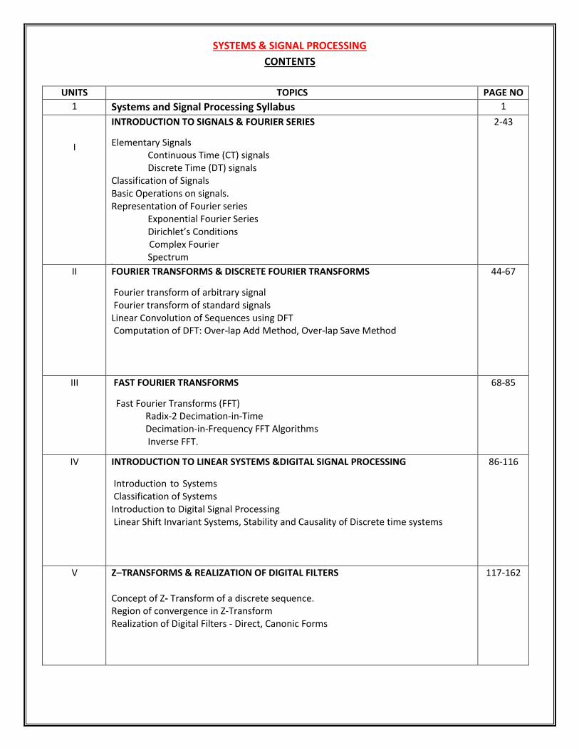
CONTENTS
UNITS TOPICS PAGE NO
1 Systems and Signal Processing Syllabus 1
I
INTRODUCTION TO SIGNALS & FOURIER SERIES
Elementary Signals Continuous Time (CT) signals Discrete Time (DT) signals
Classification of Signals Basic Operations on signals. Representation of Fourier series
Exponential Fourier Series Dirichlet’s Conditions
Complex Fourier Spectrum
{{{
2-43
II FOURIER TRANSFORMS & DISCRETE FOURIER TRANSFORMS
Fourier transform of arbitrary signal Fourier transform of standard signals Linear Convolution of Sequences using DFT Computation of DFT: Over-lap Add Method, Over-lap Save Method
44-67
III FAST FOURIER TRANSFORMS
Fast Fourier Transforms (FFT) Radix-2 Decimation-in-Time Decimation-in-Frequency FFT Algorithms Inverse FFT.
68-85
IV INTRODUCTION TO LINEAR SYSTEMS &DIGITAL SIGNAL PROCESSING
Introduction to Systems Classification of Systems Introduction to Digital Signal Processing Linear Shift Invariant Systems, Stability and Causality of Discrete time systems
86-116
V Z–TRANSFORMS & REALIZATION OF DIGITAL FILTERS
Concept of Z- Transform of a discrete sequence. Region of convergence in Z-Transform Realization of Digital Filters - Direct, Canonic Forms
117-162

1
MALLA REDDY COLLEGE OF ENGINEERING AND TECHNOLOGY
III B.Tech EEE IISEM
OBJECTIVES:
(PROFESSIONAL ELECTIVE – II)
SYSTEMS & SIGNAL PROCESSING SUBJECT CODE (R18A0463)
The main objectives of the course are:
• To understand the basic concepts of basic elementary signals and Fourier Series representation.
• To Master the representation of signals in the frequency domain using Fourier transforms and Discrete Fourier transform
• To learn the Mathematical and computational skills needed to understand the principal of Linear System and digital signal processing fundamentals.
• To understand the implementation of the DFT in terms of the FFT. • To learn the Realization of Digital Filters
UNIT I:
INTRODUCTION TO SIGNALS: Elementary Signals- Continuous Time (CT) signals, Discrete Time (DT) signals, Classification of Signals, Basic Operations on signals. FOURIER SERIES: Exponential Fourier Series, Dirichlet’s conditions, Complex Fourier Spectrum. UNIT II:
FOURIER TRANSFORMS: Fourier transform of arbitrary signal, Fourier transform of standard signals. Discrete Fourier Transforms: Properties of DFT. Linear Convolution of Sequences using DFT. Computation of DFT: Over-lap Add Method, Over-lap Save Method. UNIT III:
FAST FOURIER TRANSFORMS: Fast Fourier Transforms (FFT) - Radix-2 Decimation-in-Time and
Decimation-in-Frequency FFT Algorithms, Inverse FFT.
UNIT IV:
INTRODUCTION TO LINEAR SYSTEMS: Introduction to Systems, Classification of Systems, INTRODUCTION TO DIGITAL SIGNAL PROCESSING: Introduction to Digital Signal Processing, Linear Shift Invariant Systems, Stability, and Causality of Discrete time systems UNIT V:
Z–TRANSFORMS: Concept of Z- Transform of a discrete sequence. Region of convergence in
Z- Transform REALIZATION OF DIGITAL FILTERS: Realization of Digital Filters - Direct, Canonic forms. TEXT BOOKS:
1. Signals, Systems & Communications - B.P. Lathi, BS Publications, 2003. 2. Signals and Systems – A. Anand Kumar, PHI Publications, 3rd edition.
2
3. Digital Signal Processing, Principles, Algorithms, and Applications: John G. Proakis, Dimitris G. Manolakis, Pearson Education / PHI, 2007.
4. Digital Signal ProcessingA. Anand Kumar, PHI Publications.
REFERENCE BOOKS:
1. Signals & Systems - Simon Haykin and Van Veen,Wiley, 2nd Edition. 2. Fundamentals of Signals and Systems Michel J. Robert, MGH International Edition, 2008. 3. Digital Signal Processing – S.Salivahanan, A.Vallavaraj and C.Gnanapriya, TMH, 2009. 4. Discrete Time Signal Processing – A. V. Oppenheim and R.W. Schaffer, PHI, 2009.
OUTCOMES:
After completion of the course, the student would be able to:
• Understand the basic elementary signals.
• Represent signals in the frequency domain using Fourier Series, Discrete Fourier series, Fourier transform and Discrete Fourier transform techniques.
• Understand the principle of Linear System and digital signal processing fundamentals.
• Implement DFT of any signal using FFT algorithm.
• Realize Digital Filters

3
UNIT I
INTRODUCTION TO SIGNALS& FOURIER SERIES
➢ Elementary Signals
Continuous Time (CT) signals
Discrete Time (DT) signals
➢ Classification of Signals ➢ Basic Operations on signals. ➢ Representation of Fourier Series
Exponential Fourier Series
Discrete Fourier Series
Properties of Discrete Fourier Series

4
1. INTRODUCTION
Anything that carries information can be called a signal. Signals constitute an important part of
our daily life. A signal is defined as a single-valued function of one or more independent variable
which contains some information. A signal may also defined be defined as any physical quantity
that varies with time, space or any other independent variable. A signal may be represented in
time domain or frequency domain. A signal can be function of one or more independent variable.
A signal may be a function of time, temperature, pressure, distance etc. If a signal depends on
only one independent variable, it is called a one dimensional signal and If a signal depends on two
independent variable, it is called a two-dimensional signal. Examples of on1D and 2D signals are
shown in figure.
Examples of signals include: 1. A voltage signal: voltage across two points varying as a function of time. 2. A force pattern: force varying as a function of 2-dimensional space. 3. A photograph: color and intensity as a function of 2-dimensional space 4. A video signal: color and intensity as a function of 2-dimensional space and time
Figure 1.1 a) One Dimensional EEG Signal b) One Dimensional DNA Signal c)Two Dimensional Signal

5
ELEMENTARY SIGNALS
There are several elementary signals which plays vital role in the study of signals and systems.
These elementary signals serve as basic building blocks for the construction of more complex
signals. Infact, these elementary signals may be used to model a large number of physical signals
which occur in nature. These elementary signals are also called standard signals.
The standard signals are:
1. Unit step function
2. Unit ramp function
3. Unit parabolic function
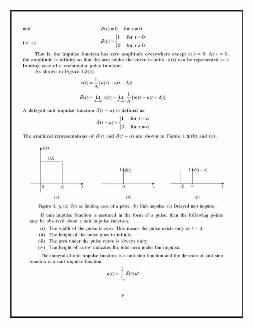
4. Unit impulse function
5. Sinusoidal function
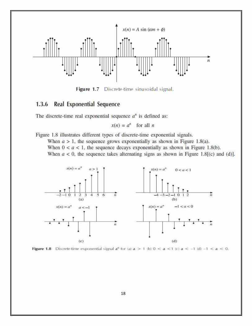
6. Real exponential function
7. Complex exponential function, etc
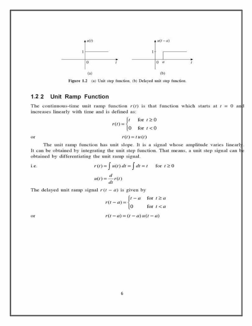
1.2.1 Unit Step Function
The step function is an important signal used for analysis of many systems. The step function is
that type of elementary function which exists only for positive time and is zero for negative time.
It is equivalent to applying a signal whose amplitude suddenly changes and remains constant
forever after application.
6

7

8
9

10

11

12

13

14

15

16

17
18

19
Classification of the Signals:
Based upon their nature characteristics in the time domain, the signals may be broadly
classified as under (a) Continuous0time signals
(b) Discrete –time signals
• Continuous-Time (CT) Signals: They may be de ned as continuous in time and continuous
in amplitude as shown in Figure 1.5.1. Ex: Speech, audio signals etc..
• Discrete Time (DT) Signals: Discretized in time and Continuous in amplitude. They may also be defined as sampled version of continuous time signals. Ex: Rail track signals.

20
• Digital Signals: Discretized in time and quantized in amplitude. They may also be defined as quantized version of discrete signals.
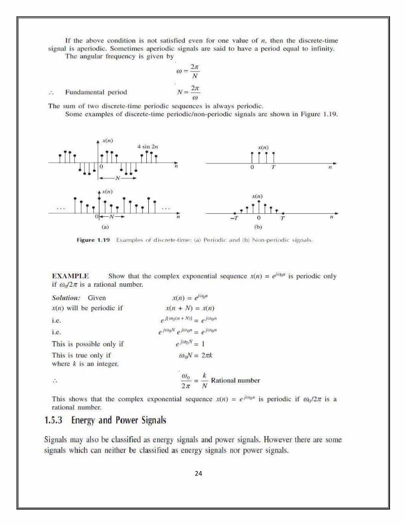
x(n) = x (n + N0) (1.2)
Figure :Description of Continuous, Discrete and Digital Signals
Both Continuous, Discrete and Digital Signals may be further classified into several categories
depending upon the criteria and for its classification. Broadly the signals are classified into the
following categories
1. Deterministic and Random signals
2. Periodic and Aperiodic Signals
3. Even and Odd Signals
4. Power and Energy Signals
5. Causal and non causal
Continuous-time and Discrete-time Signals:
Deterministic and Random signal A deterministic signal is a signal in which each value of the signal is fixed and can be determined by a mathematical expression, rule, or table. Because of this the future values of the signal can be calculated from past values with complete confidence. On the other hand, a random signal has lot of uncertainty about its behavior. The future values of a random signal cannot be accurately predicted and can usually only be guessed based on the averages of sets of signals.
Periodic Signals
A CT signal x(t) is said to be periodic if it satisfies the following condition
21
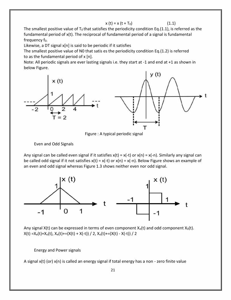
x (t) = x (t + T0) (1.1) The smallest positive value of T0 that satisfies the periodicity condition Eq.(1.1), is referred as the fundamental period of x(t). The reciprocal of fundamental period of a signal is fundamental frequency f0. Likewise, a DT signal x[n] is said to be periodic if it satisfies The smallest positive value of N0 that satis es the periodicity condition Eq.(1.2) is referred to as the fundamental period of x [n]. Note: All periodic signals are ever lasting signals i.e. they start at -1 and end at +1 as shown in below Figure.
Figure : A typical periodic signal
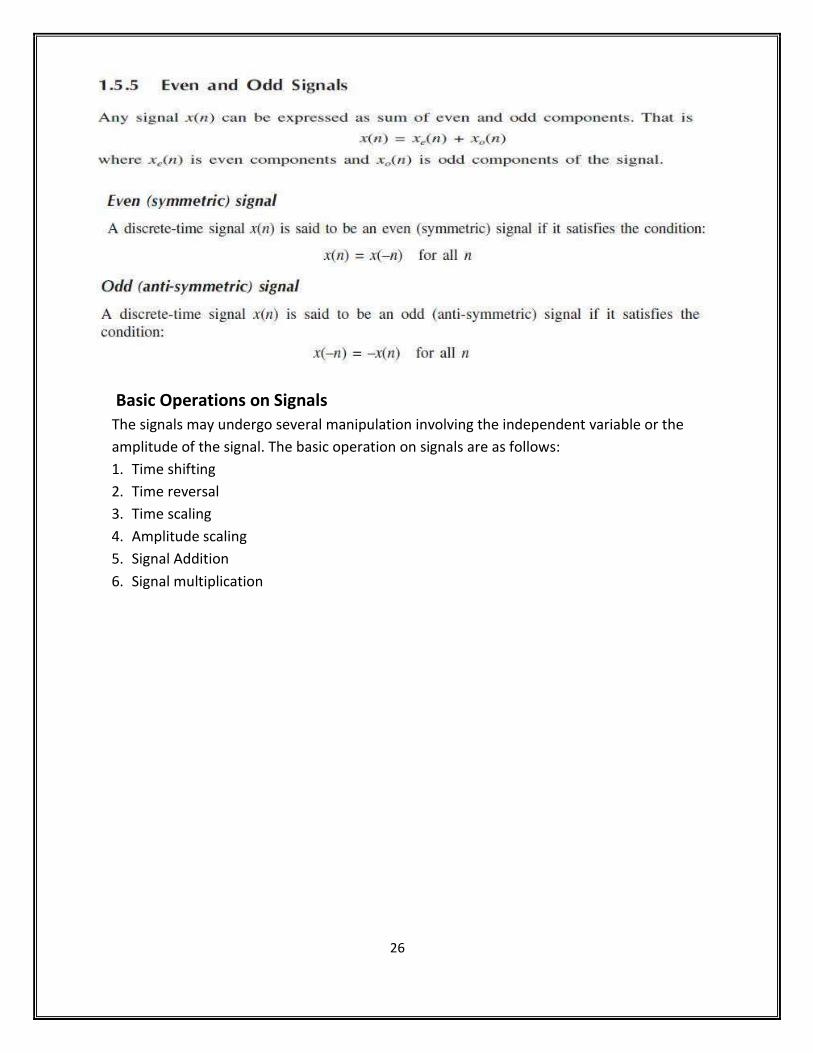
Even and Odd Signals
Any signal can be called even signal if it satisfies x(t) = x(-t) or x(n) = x(-n). Similarly any signal can be called odd signal if it not satisfies x(t) = x(-t) or x(n) = x(-n). Below Figure shows an example of an even and odd signal whereas Figure 1.3 shows neither even nor odd signal.
Any signal X(t) can be expressed in terms of even component Xe(t) and odd component X0(t). X(t) =Xe(t)+Xo(t), Xe(t)+=(X(t) + X(-t)) / 2, Xo(t)+=(X(t) - X(-t)) / 2
Energy and Power signals
A signal x(t) (or) x(n) is called an energy signal if total energy has a non - zero finite value

22
i.e. 0 < Ex < 1 and Pavg = 0 A signal is called a power signal if it has non - zero nite power i.e. 0 < Px < 1 and E = 1. A signal can't be both an energy and power signal simultaneously. The term instantaneous power is reserved for the true rate of change of energy in a system. All periodic signals are power signals and all finite durations signals are energy signals.
Causal and non causal
A continuous time signal xt) is said to be causal if x(t)=0 fort<= otherwise the signal is non causal

23
24

25
26
Basic Operations on Signals
The signals may undergo several manipulation involving the independent variable or the
amplitude of the signal. The basic operation on signals are as follows:
1. Time shifting
2. Time reversal
3. Time scaling
4. Amplitude scaling
5. Signal Addition
6. Signal multiplication

27

28

29

30

31

32

33

34

35

36
37

38
FOURIER SERIES
INTRODUCTION:
The representation of signals over a certain interval of time in terms of the linear combination of
orthogonal functions is called Fourier series. The Fourier analysis is also sometimes called the
harmonic analysis. Fourier series is applicable only for periodic signals. It cannot be applied to
non periodic signals. A periodic signal is one which repeats itself at regular intervals of time, i.e
periodically over -∞ to ∞. Three important classes of Fourier series methods are available. They
are
1. Trigonometric Form
2. Exponential Form
3. Cosine Form
In the representation of signals over a certain interval of time in terms of the linear combination
of orthogonal functions, if the orthogonal functions are exponential functions, then it is called
exponential Fourier series. Similarly, in the representation of signals over a certain interval of
time in terms of the linear combination of orthogonal functions, if the orthogonal functions are
trigonometric functions, then it is called trigonometric Fourier series.
Exponential Fourier series: The exponential Fourier series is the most widely used form of Fourier series. In this,
the function x(t) is expressed as a weighted sum of the complex exponential functions. The
complex exponential form is more general and usually more convenient and more compact. So, it

39
is used almost exclusively, and it finds extensive application in communication theory.
1) Obtain the exponential Fourier Series for the wave form shown in below figure
Solution: The periodic waveform shown in fig with a period T= 2π can be expressed as:
2) Find the exponential Fourier series for the full wave rectified sine wave given in below figure.

40

41
Complex Fourier Spectrum
The Fourier spectrum of a periodic signal x(t) is a plot of its Fourier coefficients versus
frequency ω. It is in two parts: (a) Amplitude spectrum and (b) phase spectrum. The plot of
the amplitude of Fourier coefficients verses frequency is known as the amplitude spectra, and
the plot of the phase of Fourier coefficients verses frequency is known as phase spectra. The
two plots together are known as Fourier frequency spectra of x(t).This type of representation
is also called frequency domain representation. The Fourier spectrum exists only at discrete
frequencies nωo, where n=0,1,2,….. Hence it is known as discrete spectrum or line spectrum.
The envelope of the spectrum depends only upon the pulse shape, but not upon the period of
repetition.
The below figure (a) represents the spectrum of a trigonometric Fourier series extending
from 0 to ∞, producing a one-sided spectrum as no negative frequencies exist here. The figure
(b) represents the spectrum of a complex exponential Fourier series extending from -∞𝑡𝑜∞,
producing a two-sided spectrum. The amplitude spectrum of the exponential Fourier series is
symmetrical Fourier series is symmetrical about the vertical axis. This is true for all periodic
functions.
Fig: Complex frequency spectrum for (a) Trigonometric Fourier series and (b) complex
exponential Fourier series. If Cn is a general complex number, then
Cn = Cn⎸𝑒𝑗𝜃𝑛& C-n = Cn⎸𝑒−𝑗𝜃𝑛&Cn = C-n
The magnitude spectrum is symmetrical about the vertical axis passing through
the origin, and the phase spectrum is ant symmetrical about the vertical axis passing through the
origin. So the magnitude spectrum exhibits even symmetry and phase spectrum exhibits odd
symmetry. When x(t) is real , then C- , the complex conjugate of Cn.

42
DISCRETE FOURIER SERIES
The Fourier series representation of a periodic discrete-time sequence is called discrete Fourier
series(DFS).Consider the discrete time signal x(n) that is periodic with period N defined by
x(n)=x(n+KN) for any integer value of k. The periodic function x(n) can be synthesized as a linear
combination of complex exponentials.
Exponential form of Discrete Fourier Series
A real periodic discrete time signal x(n) of period N can be expressed as a weighted sum of
complex exponential sequences. The exponential form of the Fourier series for a periodic discrete
time signal is given by

43
44
UNIT-II
FOURIER TRANSFORMS & DISCRETE FOURIER TRANSFORMS
➢ Fourier transform of arbitrary signal, ➢ Fourier transform of standard signals ➢ Properties of Fourier Transform. ➢ Discrete Fourier Transform ➢ Properties of DFT ➢ Linear Convolution of Sequences using DFT ➢ Computation of DFT: Over-lap Add Method & Over-lap Save Method.

45
FOURIER TRANSFORM
INTRODUCTION:
Using exponential form of Fourier series, any continuous –time periodic signal x(t) can be represented as a
linear combination of complex exponentials and the Fourier coefficients are discrete. Fourier series can
deal only with the periodic signals. This is the major drawback of Fourier series. However, all the naturally
produced signals which need processing will be in the form of non-periodic or aperiodic signals. Therefore,
the applicability of the Fourier series is limited.
Fourier Transform is a transformation technique which transforms signals from the continuous-time
domain to the corresponding frequency domain and vice versa and which applies for both periodic as well
as aperiodic signals. Fourier transform can be developed by finding the Fourier series of a periodic
function and then tending to infinity. The Fourier Transform derived in this chapter is called the
continuous-time Fourier transform (CTFT) . The Fourier Transform is an extremely useful mathematical
tool and is extensively used in the analysis of linear time –invariant (LTI) systems, cryptography, signal
analysis, signal processing, astronomy etc. Several applications ranging from RADAR to spread spectrum
communication employ Fourier transform.
The magnitude of X(w) is given by
The phase of X(w) is given by
X (w) =
= tan−1 X I (w)
XR (w)
The plot of X (w) versus w is known as amplitude spectrum and the plot of versus w is known as
phase spectrum. The amplitude spectrum and phase spectrum together is called frequency spectrum.
EXISTANCE FOURIER TRANSFORM:
The Fourier Transform does not exist for all aperiodic functions. The conditions for function x(t) to have
Fourier Transform, called Dirichlet’s conditions are:
1. x(t) is absolutely integrable over the interval- ∞ to ∞, that is
x(t)dt −
2.x(t) has a finite number of discontinuities in every finite time interval, Further, each of these
discontinuities must be finite.
3.x(t) has a finite number of maxima and minima in every finite time interval.
Dirichlet’s condition is a sufficient condition but necessary condition. This means, Fourier transform will
definitely exist for functions which satisfy these conditions. On the other hand, in some cases, Fourier
transform can be found with the use of impulses even for functions like step functions, sinusoidal
function, etc which do not satisfy the convergence condition.
X (w) + X (w) 2 2
R I
X (w)
X (w)

46
FOURIER TRANSFORM OF STANDARD SIGNALS
1. Impulse Function
Given δ ,
Then
= e−jωt⎸t=0 = 1
Hence , the Fourier Transform of a unit impulse function is unity.
w
w w
The impulse functions with its magnitude and phase spectra are shown in below figure:
Similarly,
2. Single Sided Real exponential function 𝐞−𝐚𝐭𝐮(𝐭)
Given
Then

47
Now,
Figure shows the single-sided exponential function with its magnitude and phase spectra.
3. Double sided real exponential function 𝐞−𝐚𝐭
Given
or
48
Where
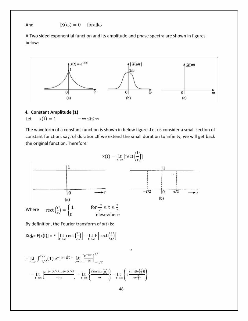
And
A Two sided exponential function and its amplitude and phase spectra are shown in figures
below:
4. Constant Amplitude (1)
Let ∞ ≤t≤ ∞
The waveform of a constant function is shown in below figure .Let us consider a small section of
constant function, say, of duration .If we extend the small duration to infinity, we will get back
the original function.Therefore
By definition, the Fourier transform of x(t) is:
X( ) = F[x(t)] = F
dt =

49
Using the sampling property of the delta function , we get
X(
5. Signum function (sgn(t))
The signum function is denoted by sgn(t) and is defined by
sgn(t) =
This function is not absolutely integrable. So we cannot directly find its Fourier transform.
Therefore, let us consider the function e−a⎹t⎸sgn(t) and substitute the limit a 0 to obtain the
above sgn(t)
Given x(t) = sgn(t) = sgn(t) =
X( ) = F[sgn(t)] = dt
and
Figure below shows the signum function and its magnitude and phase spectra

50
6. Unit step function u(t)
The unit step function is defined by
u(t)
since the unit step function is not absolutely integrable, we cannot directly find its Fourier
transform. So express the unit step function in terms of signum function as: u(t) =
x(t)= u(t) =
X( ) = F[u(t)] = F
We know that F[1] = 2𝜋𝛿(𝜔) and F[sgn(t)] =
F[u(t)]=
u(t)
∴⎹X(⍵)⎸=∞ at ⍵=0 and is equal to 0 at ⍵=−∞ and ⍵=∞
7. Rectangular pulse ( Gate pulse) or rect
Consider a rectangular pulse as shown in below figure. This is called a unit gate function and is
defined as
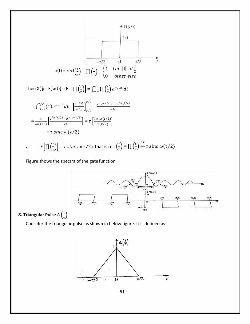
51
x(t) = rect
Then X( ) = F[ x(t)] = F
=
∴ F , that is rect
Figure shows the spectra of the gate function
8. Triangular Pulse
Consider the triangular pulse as shown in below figure. It is defined as:

52
x
i.e. as x(t) =
Then X( ) = F[ x(t)] = F
F Or
Figure shows the amplitude spectrum of a triangular pulse.
53
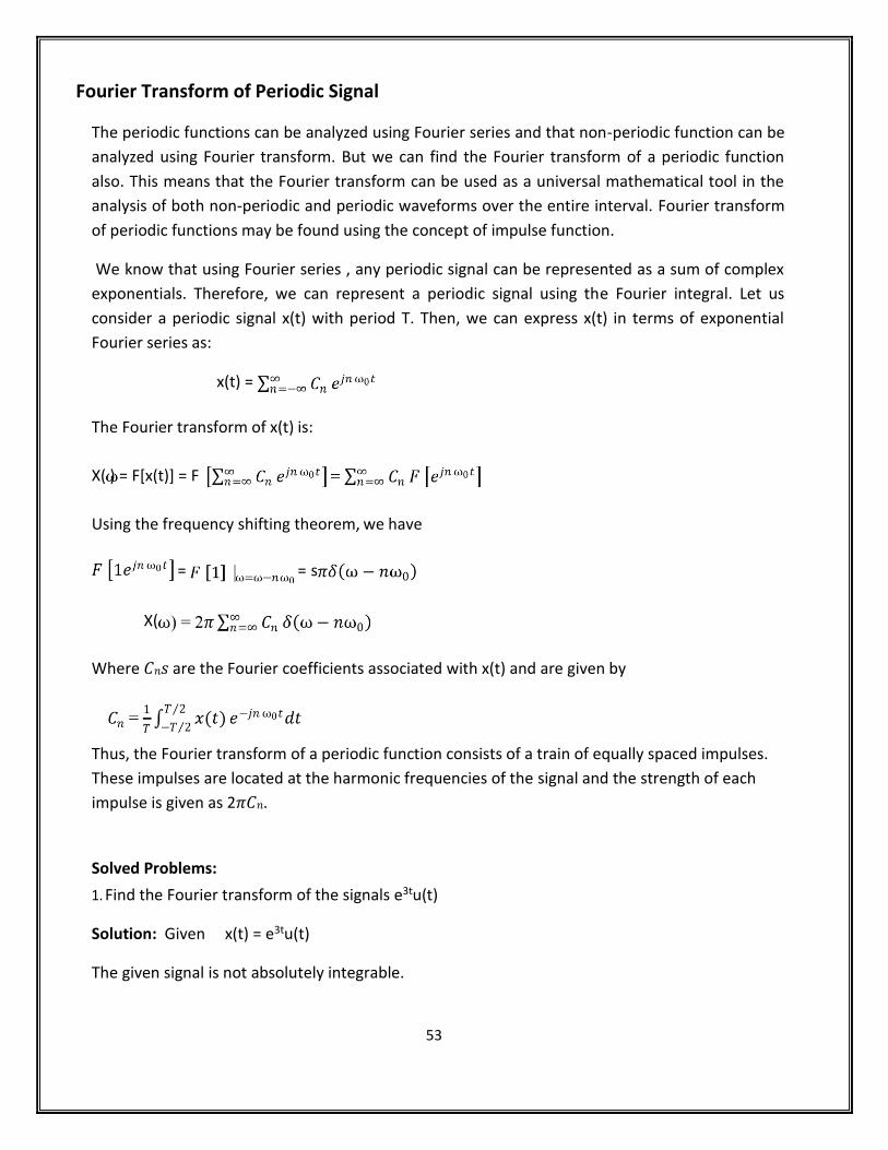
Fourier Transform of Periodic Signal
The periodic functions can be analyzed using Fourier series and that non-periodic function can be
analyzed using Fourier transform. But we can find the Fourier transform of a periodic function
also. This means that the Fourier transform can be used as a universal mathematical tool in the
analysis of both non-periodic and periodic waveforms over the entire interval. Fourier transform
of periodic functions may be found using the concept of impulse function.
We know that using Fourier series , any periodic signal can be represented as a sum of complex
exponentials. Therefore, we can represent a periodic signal using the Fourier integral. Let us
consider a periodic signal x(t) with period T. Then, we can express x(t) in terms of exponential
Fourier series as:
x(t) =
The Fourier transform of x(t) is:
X( ) = F[x(t)] = F
Using the frequency shifting theorem, we have
= = s
X(
Where 𝐶𝑛𝑠 are the Fourier coefficients associated with x(t) and are given by
Thus, the Fourier transform of a periodic function consists of a train of equally spaced impulses.
These impulses are located at the harmonic frequencies of the signal and the strength of each
impulse is given as 2𝜋𝐶𝑛.
Solved Problems:
1. Find the Fourier transform of the signals e3tu(t)
Solution: Given x(t) = e3tu(t)
The given signal is not absolutely integrable.

54
That is .
Therefore, Fourier transform of x(t) = e3tu(t) does not exist.
2. Find the Fourier transform of the signals cosωotu(t)
Solution:
Given x(t) = cosωot u(t)
i.e. u(t)
X( ) = F[cosωot u(t)] = dt
With impulses of strength at ω=ωo and ω=−ωo
X(
3: Find the Fourier transform of the signals sinωot u(t)
Solution:
Given x(t) = sinωot u(t)
i.e. u(t)
X( ) = F[sinωot u(t)] = dt

55
With impulses of strength at ω=ωo and ω=−ωo
X(
4. Find the Fourier transform of the signals e−tsin5t u(t)
Solution:
Given x(t) = e−tsin5t u(t)
x(t) = u(t)
X( ) = F[e−t sin5t u(t)]
)u(t)] e−jωt dt
[neglecting impulses]
5. Find the Fourier transform of the signals e−2tcos5t u(t)
Solution:
Given x(t) = e−2tcos5t u(t)
x(t) = u(t)
X( ) = F[e−2t cos5t u(t)]

56
)u(t)] e−jωt dt
[neglecting impulses]

57
DISCRETE FOURIER TRANSFORM

58

59

60

61

62

63
64

65
66

67

68
UNIT III
FAST FOURIER TRANSFORM
➢ Decimation-in-Time FFT Algorithm ➢ Decimation-in-Frequency FFT Algorithms ➢ Decimation-in-Time Inverse FFT. ➢ Decimation-in-Frequency Inverse FFT

69
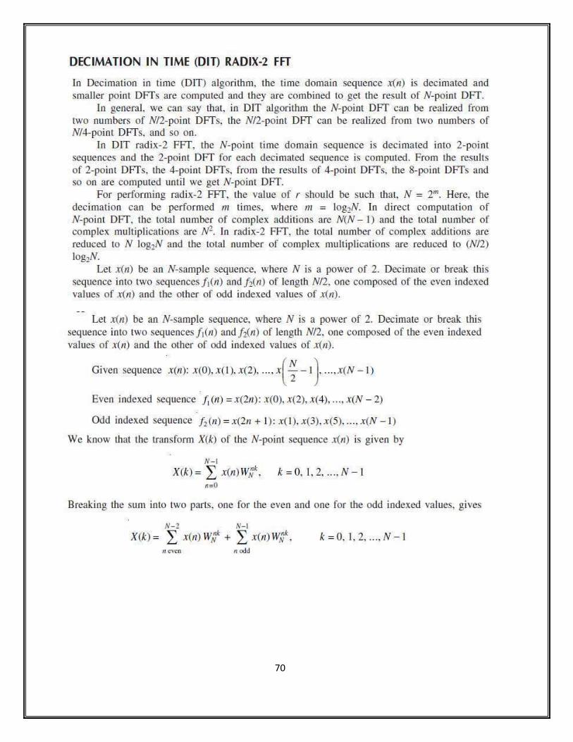
70

71

72

73

74

75

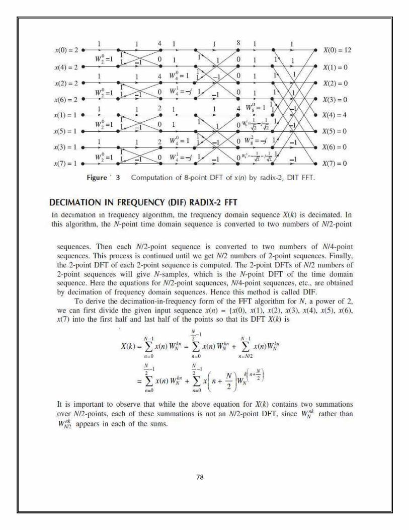
76
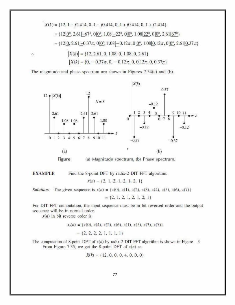
77
78
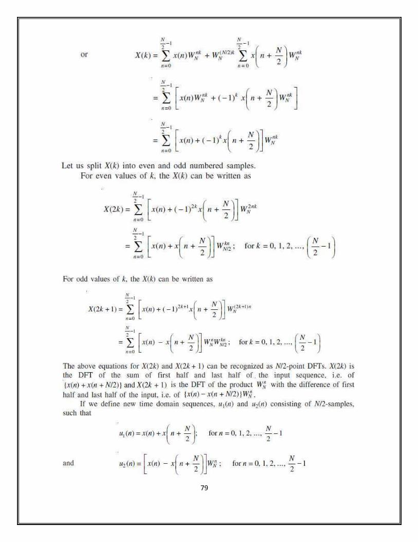
79
80
81

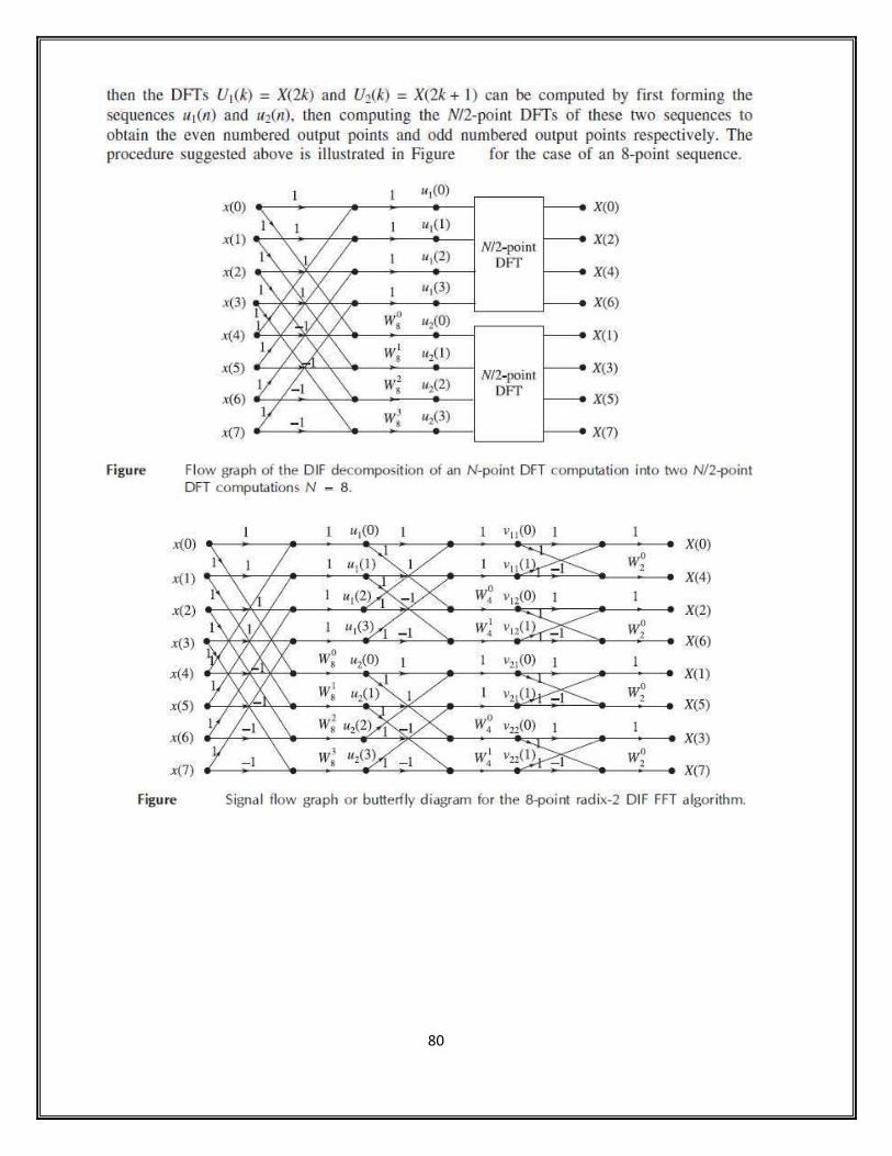
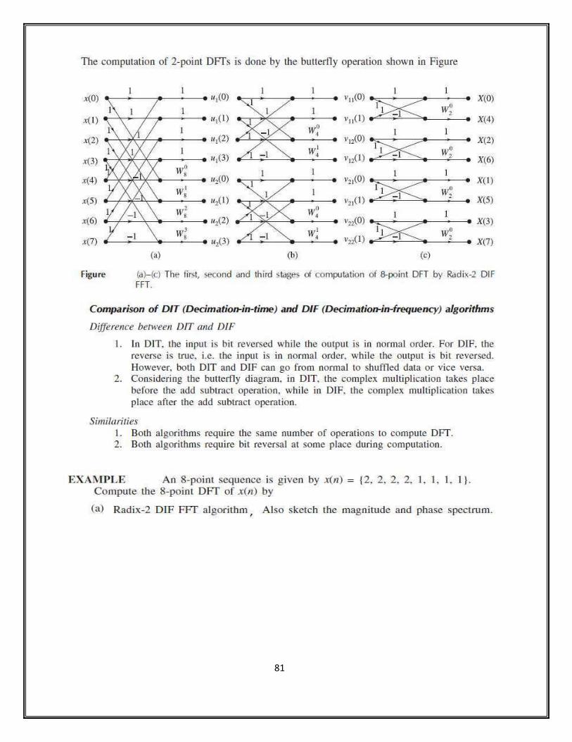
82
83

84

85
86
UNIT IV
INTRODUCTION TO LINEAR SYSTEMS & DIGITAL SIGNAL PROCESSING
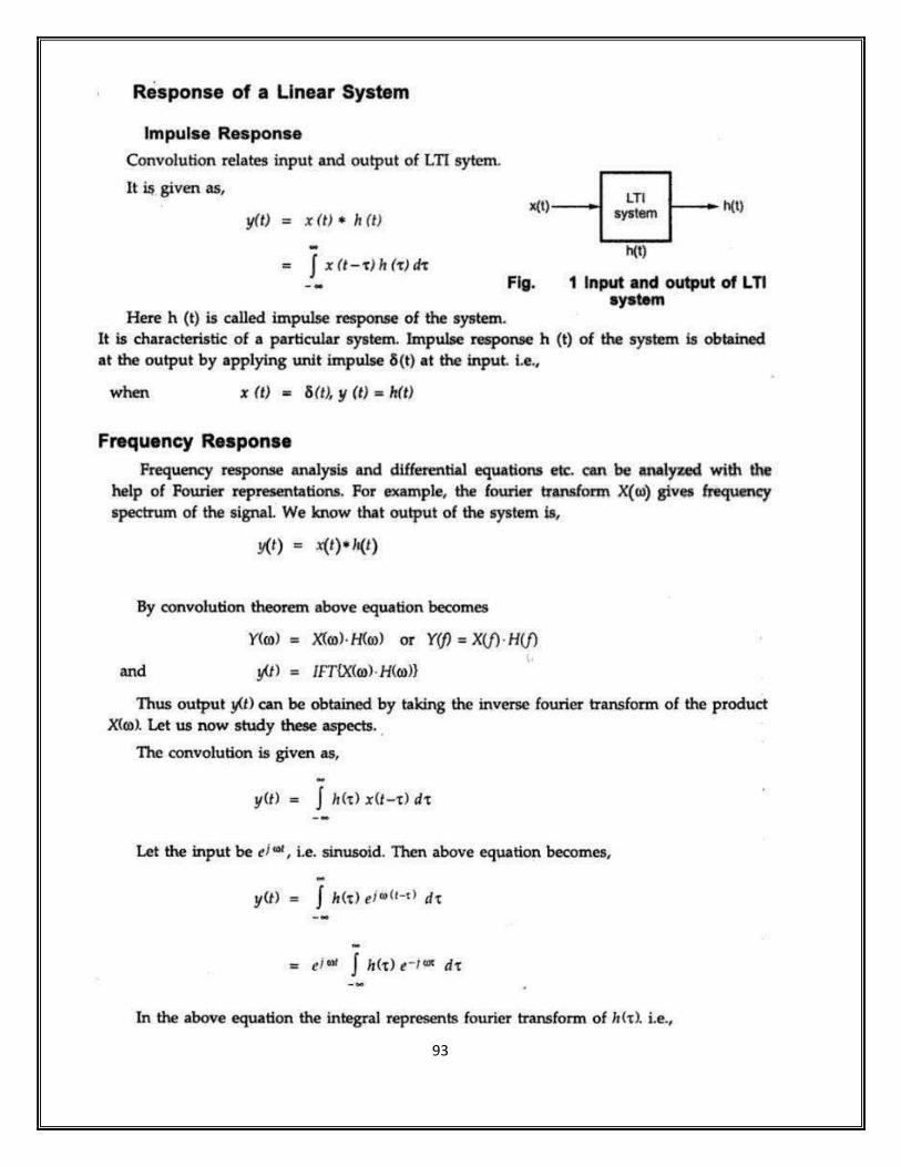
➢ Introduction to Systems ➢ Classification of Systems ➢ Impulse response ➢ Transfer function of a LTI system. ➢ Introduction to Digital Signal Processing ➢ Linear Shift Invariant Systems, ➢ Stability and Causality of Discrete time systems

87
INTRODUCTION TO LINEAR SYSTEMS

88

89

90

91
92
93

94

95

96

97
98

99
INTRODUCTION TO DIGITAL SIGNAL PROCESSING
Introduction

100

101

102
103

104

105
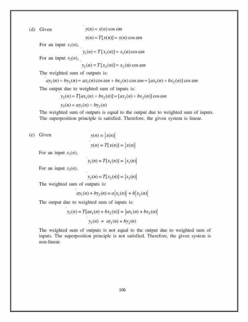
106

107

108

109
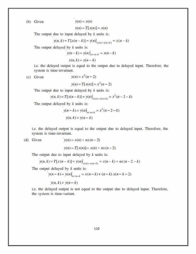
110
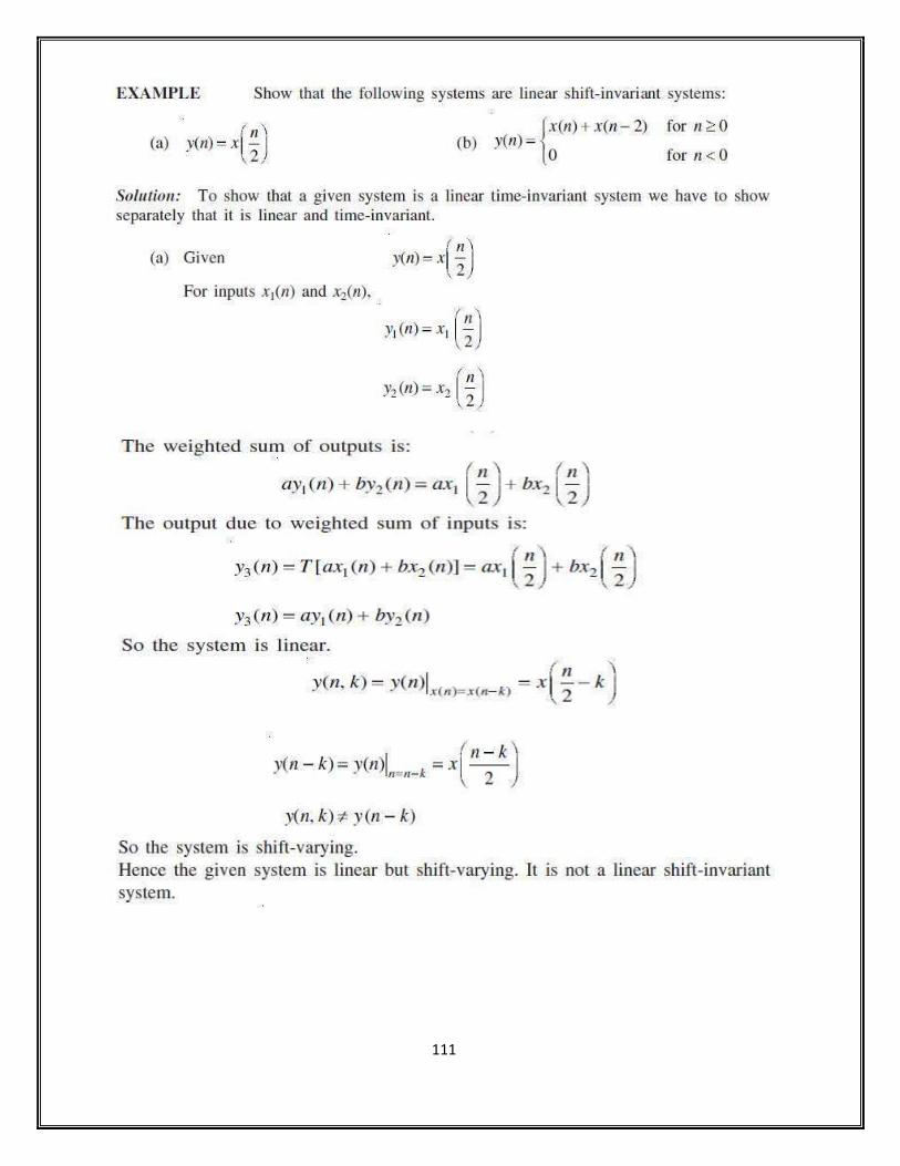
111

112

113

114

115
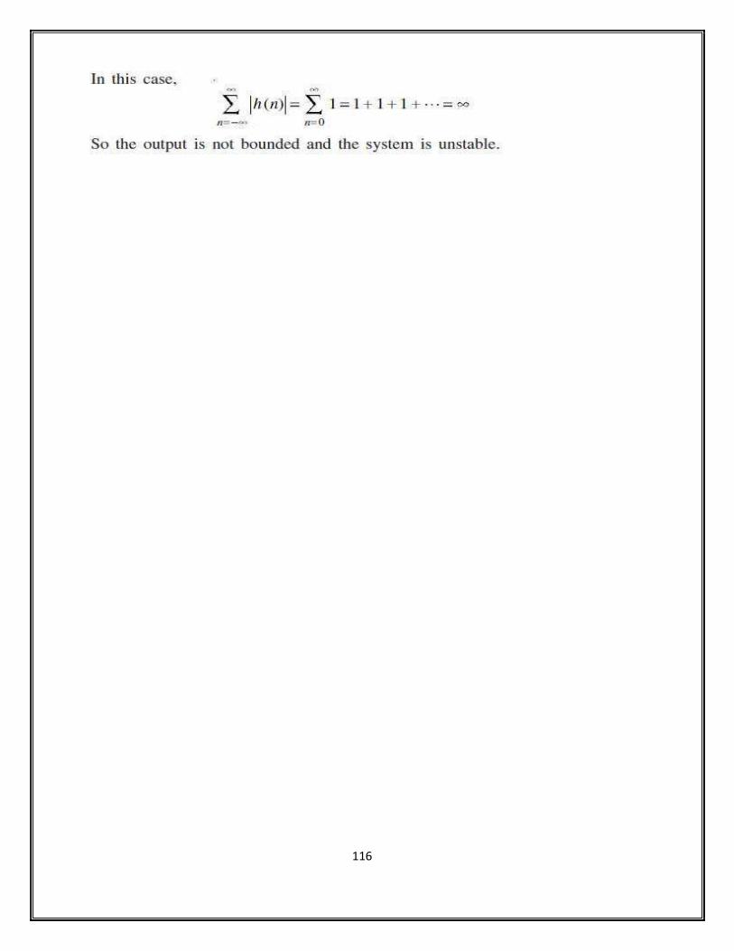
116
117
UNIT V
Z–TRANSFORMS & REALIZATION OF DIGITAL FILTERS
➢ Concept of Z- Transform of a discrete sequence. ➢ Region of convergence in Z-Transform ➢ Inverse Z- Transform. ➢ Solution of Difference Equations Using Z-Transform ➢ Realization of Digital Filters - Direct and Canonic forms.

118
INTRODUCTION

119

120
121
122

123
124

125

126
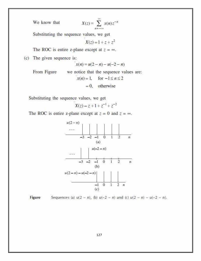
127

128

129

130

131

132
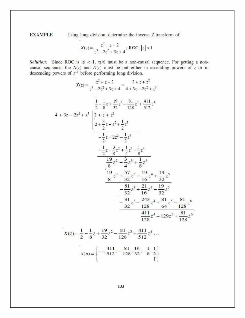
133

134
\

135
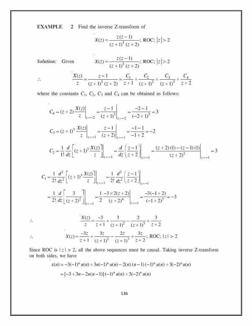
136

137
138

139

140
\

141
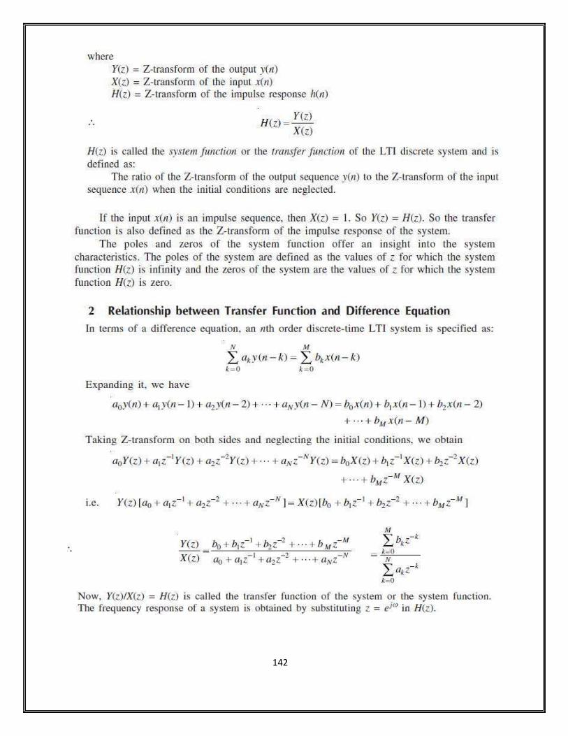
142

143

144
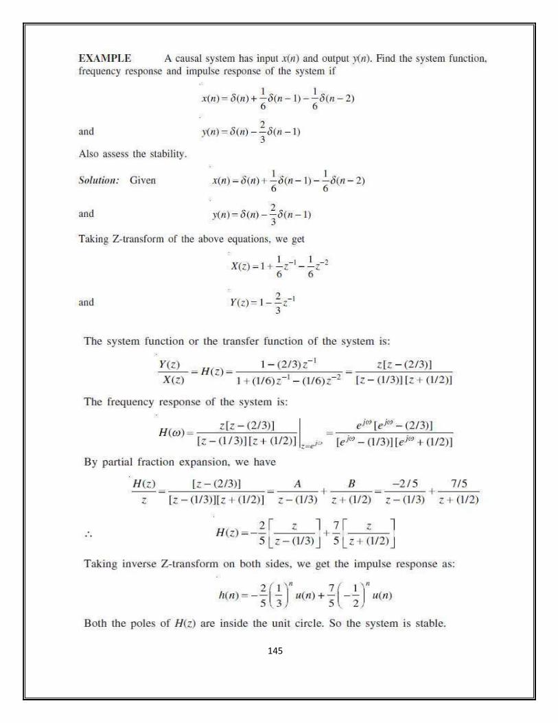
145

146
REALIZATION OF DIGITAL FILTERS

147

148
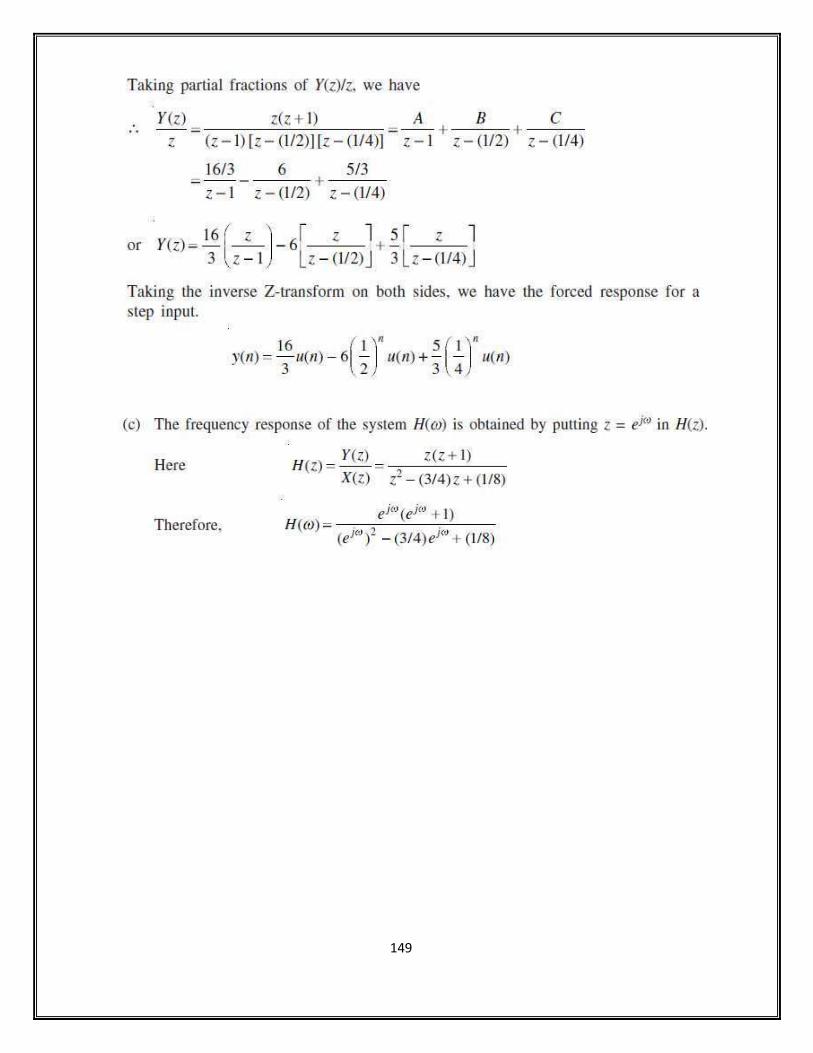
149

150

151

152

153

154

155

156

157

158

159

160
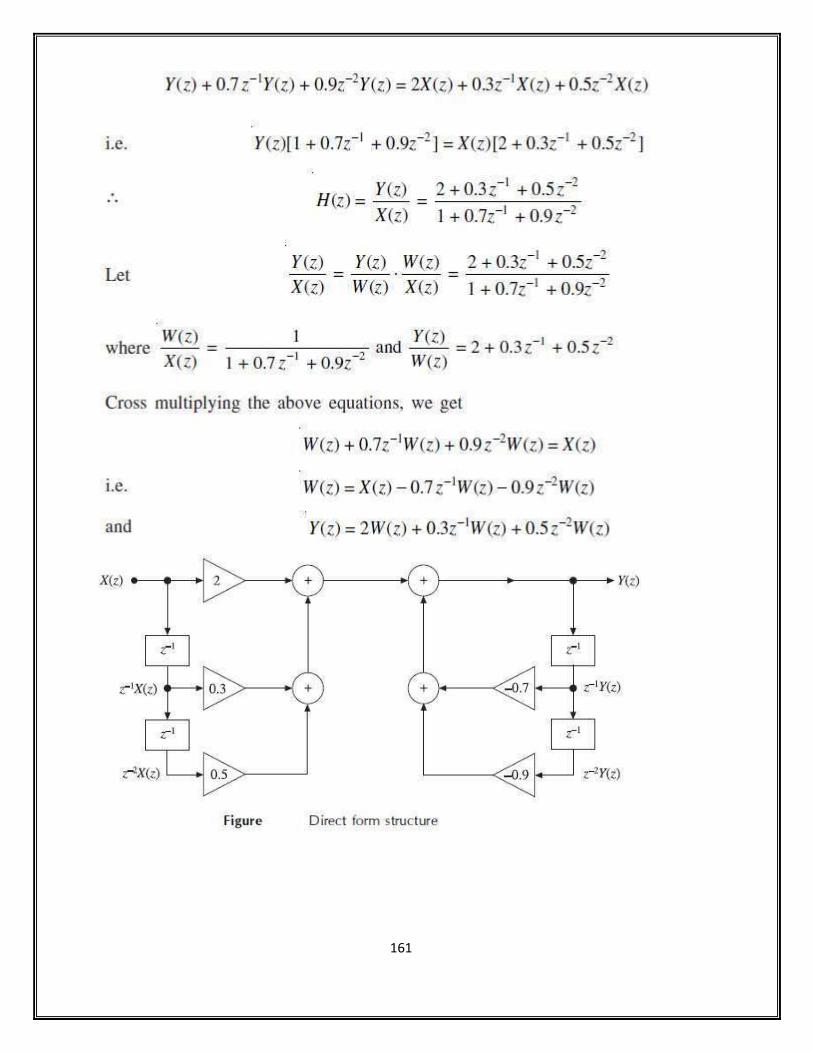
161

162