Signal Processing With Scilab
74
-
Upload
khangminh22 -
Category
Documents
-
view
1 -
download
0
Transcript of Signal Processing With Scilab


Signal
Processing
With
Scilab
Scilab Group
-1
100
101
102
103
10
-160
-150
-140
-130
-120
-110
-100
-90Magnitude
Hz
db
-1
100
101
102
103
10
-180
-90
0Phase
Hz
degrees
4.64 7.44 10.23 13.02 15.82 18.61 21.41 24.20 27.00 29.79 32.58
0.19
1.51
2.84
4.16
5.49
6.81
8.14
9.47
10.79
12.12
13.44
×
×
×
×
×
×
×
××
×
×
⊕
⊕
⊕
⊕
⊕
⊕
⊕⊕
⊕ ⊕⊕
-->a=-2*%pi;b=1;c=18*%pi;d=1;
-->sl=syslin('c',a,b,c,d);
-->bode(sl,.1,100);
-->s=poly(0,'s');
-->S1=s+2*%pi*(15+100*%i);
-->S2=s+2*%pi*(15-100*%i);
-->h1=1/real(S1*S2)
h1 =
1-------------------------
2403666.82 + 188.49556s + s
-->h1=syslin('c',h1);
-->bode(h1,10,1000,.01);
-->h2=ss2tf(sl);
-->bode(h1*h2,.1,1000,.01);

SIGNAL
PROCESSING
WITH
Lab
Scilab GroupINRIA Meta2 Project/ENPC Cergrene
INRIA - Unit�e de recherche de Rocquencourt - Projet Meta2Domaine de Voluceau - Rocquencourt - B.P. 105 - 78153 Le Chesnay Cedex (France)E-mail : [email protected]

Acknowledgement
This document is the new version of a primary work by Carey Bunks, Fran�cois Delebecque,Georges Le Vey and Serge Steer

Contents
1 Description of the Basic Tools 1
1.1 Introduction : : : : : : : : : : : : : : : : : : : : : : : : : : : : : : : : : : : : : : : : : 11.2 Signals : : : : : : : : : : : : : : : : : : : : : : : : : : : : : : : : : : : : : : : : : : : : 1
1.2.1 Saving, Loading, Reading, and Writing Files : : : : : : : : : : : : : : : : : : 21.2.2 Simulation of Random Signals : : : : : : : : : : : : : : : : : : : : : : : : : : 3
1.3 Polynomials and System Transfer Functions : : : : : : : : : : : : : : : : : : : : : : : 41.3.1 Evaluation of Polynomials : : : : : : : : : : : : : : : : : : : : : : : : : : : : : 81.3.2 Representation of Transfer Functions : : : : : : : : : : : : : : : : : : : : : : : 9
1.4 State Space Representation : : : : : : : : : : : : : : : : : : : : : : : : : : : : : : : : 91.5 Changing System Representation : : : : : : : : : : : : : : : : : : : : : : : : : : : : : 101.6 Interconnecting systems : : : : : : : : : : : : : : : : : : : : : : : : : : : : : : : : : : 111.7 Discretizing Continuous Systems : : : : : : : : : : : : : : : : : : : : : : : : : : : : : 111.8 Filtering of Signals : : : : : : : : : : : : : : : : : : : : : : : : : : : : : : : : : : : : : 141.9 Plotting Signals : : : : : : : : : : : : : : : : : : : : : : : : : : : : : : : : : : : : : : : 151.10 Development of Signal Processing Tools : : : : : : : : : : : : : : : : : : : : : : : : : 19
2 Representation of Signals 21
2.1 Frequency Response : : : : : : : : : : : : : : : : : : : : : : : : : : : : : : : : : : : : 212.1.1 Bode Plots : : : : : : : : : : : : : : : : : : : : : : : : : : : : : : : : : : : : : 212.1.2 Phase and Group Delay : : : : : : : : : : : : : : : : : : : : : : : : : : : : : : 272.1.3 Appendix: Lab Code Used to Generate Examples : : : : : : : : : : : : : : : 35
2.2 Sampling : : : : : : : : : : : : : : : : : : : : : : : : : : : : : : : : : : : : : : : : : : 372.3 Decimation and Interpolation : : : : : : : : : : : : : : : : : : : : : : : : : : : : : : : 41
2.3.1 Introduction : : : : : : : : : : : : : : : : : : : : : : : : : : : : : : : : : : : : 412.3.2 Interpolation : : : : : : : : : : : : : : : : : : : : : : : : : : : : : : : : : : : : 442.3.3 Decimation : : : : : : : : : : : : : : : : : : : : : : : : : : : : : : : : : : : : : 442.3.4 Interpolation and Decimation : : : : : : : : : : : : : : : : : : : : : : : : : : : 442.3.5 Examples using intdec : : : : : : : : : : : : : : : : : : : : : : : : : : : : : : 46
2.4 The DFT and the FFT : : : : : : : : : : : : : : : : : : : : : : : : : : : : : : : : : : 462.4.1 Introduction : : : : : : : : : : : : : : : : : : : : : : : : : : : : : : : : : : : : 462.4.2 Examples Using the fft Primitive : : : : : : : : : : : : : : : : : : : : : : : : 52
2.5 Convolution : : : : : : : : : : : : : : : : : : : : : : : : : : : : : : : : : : : : : : : : : 552.5.1 Introduction : : : : : : : : : : : : : : : : : : : : : : : : : : : : : : : : : : : : 552.5.2 Use of the convol function : : : : : : : : : : : : : : : : : : : : : : : : : : : : 56
2.6 The Chirp Z-Transform : : : : : : : : : : : : : : : : : : : : : : : : : : : : : : : : : : 572.6.1 Introduction : : : : : : : : : : : : : : : : : : : : : : : : : : : : : : : : : : : : 572.6.2 Calculating the CZT : : : : : : : : : : : : : : : : : : : : : : : : : : : : : : : : 582.6.3 Examples : : : : : : : : : : : : : : : : : : : : : : : : : : : : : : : : : : : : : : 59
iii

3 FIR Filters 63
3.1 Windowing Techniques : : : : : : : : : : : : : : : : : : : : : : : : : : : : : : : : : : : 63
3.1.1 Filter Types : : : : : : : : : : : : : : : : : : : : : : : : : : : : : : : : : : : : : 64
3.1.2 Choice of Windows : : : : : : : : : : : : : : : : : : : : : : : : : : : : : : : : : 66
3.1.3 How to use wfir : : : : : : : : : : : : : : : : : : : : : : : : : : : : : : : : : : 69
3.1.4 Examples : : : : : : : : : : : : : : : : : : : : : : : : : : : : : : : : : : : : : : 70
3.2 Frequency Sampling Technique : : : : : : : : : : : : : : : : : : : : : : : : : : : : : : 72
3.3 Optimal �lters : : : : : : : : : : : : : : : : : : : : : : : : : : : : : : : : : : : : : : : 74
3.3.1 Minimax Approximation : : : : : : : : : : : : : : : : : : : : : : : : : : : : : : 75
3.3.2 The Remez Algorithm : : : : : : : : : : : : : : : : : : : : : : : : : : : : : : : 76
3.3.3 Function remezb : : : : : : : : : : : : : : : : : : : : : : : : : : : : : : : : : : 77
3.3.4 Examples Using the function remezb : : : : : : : : : : : : : : : : : : : : : : : 78
3.3.5 Lab function eqfir : : : : : : : : : : : : : : : : : : : : : : : : : : : : : : : 81
4 IIR Filters 85
4.1 Analog �lters : : : : : : : : : : : : : : : : : : : : : : : : : : : : : : : : : : : : : : : : 85
4.1.1 Butterworth Filters : : : : : : : : : : : : : : : : : : : : : : : : : : : : : : : : 85
4.1.2 Chebyshev �lters : : : : : : : : : : : : : : : : : : : : : : : : : : : : : : : : : : 88
4.1.3 Elliptic �lters : : : : : : : : : : : : : : : : : : : : : : : : : : : : : : : : : : : : 94
4.2 Design of IIR Filters From Analog Filters : : : : : : : : : : : : : : : : : : : : : : : : 106
4.3 Approximation of Analog Filters : : : : : : : : : : : : : : : : : : : : : : : : : : : : : 107
4.3.1 Approximation of the Derivative : : : : : : : : : : : : : : : : : : : : : : : : : 107
4.3.2 Approximation of the Integral : : : : : : : : : : : : : : : : : : : : : : : : : : : 108
4.4 Design of Low Pass Filters : : : : : : : : : : : : : : : : : : : : : : : : : : : : : : : : : 109
4.5 Transforming Low Pass Filters : : : : : : : : : : : : : : : : : : : : : : : : : : : : : : 112
4.6 How to Use the Function iir : : : : : : : : : : : : : : : : : : : : : : : : : : : : : : : 114
4.7 Examples : : : : : : : : : : : : : : : : : : : : : : : : : : : : : : : : : : : : : : : : : : 114
4.8 Another Implementation of Digital IIR Filters : : : : : : : : : : : : : : : : : : : : : : 116
4.8.1 The eqiir function : : : : : : : : : : : : : : : : : : : : : : : : : : : : : : : : 116
4.8.2 Examples : : : : : : : : : : : : : : : : : : : : : : : : : : : : : : : : : : : : : : 117
5 Spectral Estimation 123
5.1 Estimation of Power Spectra : : : : : : : : : : : : : : : : : : : : : : : : : : : : : : : 123
5.2 The Modi�ed Periodogram Method : : : : : : : : : : : : : : : : : : : : : : : : : : : : 124
5.2.1 Example Using the pspect function : : : : : : : : : : : : : : : : : : : : : : : 125
5.3 The Correlation Method : : : : : : : : : : : : : : : : : : : : : : : : : : : : : : : : : : 128
5.3.1 Example Using the function cspect : : : : : : : : : : : : : : : : : : : : : : : 128
5.4 The Maximum Entropy Method : : : : : : : : : : : : : : : : : : : : : : : : : : : : : : 129
5.4.1 Introduction : : : : : : : : : : : : : : : : : : : : : : : : : : : : : : : : : : : : 129
5.4.2 The Maximum Entropy Spectral Estimate : : : : : : : : : : : : : : : : : : : : 130
5.4.3 The Levinson Algorithm : : : : : : : : : : : : : : : : : : : : : : : : : : : : : : 131
5.4.4 How to Use mese : : : : : : : : : : : : : : : : : : : : : : : : : : : : : : : : : : 131
5.4.5 How to Use lev : : : : : : : : : : : : : : : : : : : : : : : : : : : : : : : : : : : 132
5.4.6 Examples : : : : : : : : : : : : : : : : : : : : : : : : : : : : : : : : : : : : : : 132

v
6 Optimal Filtering and Smoothing 135
6.1 The Kalman Filter : : : : : : : : : : : : : : : : : : : : : : : : : : : : : : : : : : : : : 1356.1.1 Conditional Statistics of a Gaussian Random Vector : : : : : : : : : : : : : : 1356.1.2 Linear Systems and Gaussian Random Vectors : : : : : : : : : : : : : : : : : 1366.1.3 Recursive Estimation of Gaussian Random Vectors : : : : : : : : : : : : : : : 1376.1.4 The Kalman Filter Equations : : : : : : : : : : : : : : : : : : : : : : : : : : : 1396.1.5 Asymptotic Properties of the Kalman Filter : : : : : : : : : : : : : : : : : : : 1406.1.6 How to Use the Macro sskf : : : : : : : : : : : : : : : : : : : : : : : : : : : : 1416.1.7 An Example Using the sskf Macro : : : : : : : : : : : : : : : : : : : : : : : : 1416.1.8 How to Use the Function kalm : : : : : : : : : : : : : : : : : : : : : : : : : : 1426.1.9 Examples Using the kalm Function : : : : : : : : : : : : : : : : : : : : : : : : 143
6.2 The Square Root Kalman Filter : : : : : : : : : : : : : : : : : : : : : : : : : : : : : : 1526.2.1 The Householder Transformation : : : : : : : : : : : : : : : : : : : : : : : : : 1546.2.2 How to Use the Macro srkf : : : : : : : : : : : : : : : : : : : : : : : : : : : : 155
6.3 The Wiener Filter : : : : : : : : : : : : : : : : : : : : : : : : : : : : : : : : : : : : : 1556.3.1 Problem Formulation : : : : : : : : : : : : : : : : : : : : : : : : : : : : : : : 1566.3.2 How to Use the Function wiener : : : : : : : : : : : : : : : : : : : : : : : : : 1596.3.3 Example : : : : : : : : : : : : : : : : : : : : : : : : : : : : : : : : : : : : : : : 159
7 Optimization in �lter design 163
7.1 Optimized IIR �lters : : : : : : : : : : : : : : : : : : : : : : : : : : : : : : : : : : : : 1637.1.1 Minimum Lp design : : : : : : : : : : : : : : : : : : : : : : : : : : : : : : : : 163
7.2 Optimized FIR �lters : : : : : : : : : : : : : : : : : : : : : : : : : : : : : : : : : : : 173
8 Stochastic realization 177
8.1 The sfact primitive : : : : : : : : : : : : : : : : : : : : : : : : : : : : : : : : : : : : 1788.2 Spectral Factorization via state-space models : : : : : : : : : : : : : : : : : : : : : : 179
8.2.1 Spectral Study : : : : : : : : : : : : : : : : : : : : : : : : : : : : : : : : : : : 1798.2.2 The Filter Model : : : : : : : : : : : : : : : : : : : : : : : : : : : : : : : : : : 180
8.3 Computing the solution : : : : : : : : : : : : : : : : : : : : : : : : : : : : : : : : : : 1818.3.1 Estimation of the matrices H F G : : : : : : : : : : : : : : : : : : : : : : : : 1818.3.2 computation of the �lter : : : : : : : : : : : : : : : : : : : : : : : : : : : : : : 182
8.4 Levinson �ltering : : : : : : : : : : : : : : : : : : : : : : : : : : : : : : : : : : : : : : 1858.4.1 The Levinson algorithm : : : : : : : : : : : : : : : : : : : : : : : : : : : : : : 186
9 Time-Frequency representations of signals 189
9.0.2 The Wigner distribution : : : : : : : : : : : : : : : : : : : : : : : : : : : : : : 1899.0.3 Time-frequency spectral estimation : : : : : : : : : : : : : : : : : : : : : : : : 190
Bibliography 193

Chapter 1
Description of the Basic Tools
1.1 Introduction
The purpose of this document is to illustrate the use of the Lab software package in a signalprocessing context. We have gathered a collection of signal processing algorithms which have beenimplemented as Lab functions.
This manual is in part a pedagogical tool concerning the study of signal processing and in parta practical guide to using the signal processing tools available in Lab. For those who are alreadywell versed in the study of signal processing the tutorial parts of the manual will be of less interest.
For each signal processing tool available in the signal processing toolbox there is a tutorialsection in the manual explaining the methodology behind the technique. This section is followedby a section which describes the use of a function designed to accomplish the signal processingdescribed in the preceding sections. At this point the reader is encouraged to launch a Labsession and to consult the on-line help related to the function in order to get the precise andcomplete description (syntax, description of its functionality, examples and related functions). Thissection is in turn followed by an examples section demonstrating the use of the function. In general,the example section illustrates more clearly than the syntax section how to use the di�erent modesof the function.
In this manual the typewriter-face font is used to indicate either a function name or anexample dialogue which occurs in Lab.
Each signal processing subject is illustrated by examples and �gures which were demonstratedusing Lab. To further assist the user, there exists for each example and �gure an executable �lewhich recreates the example or �gure. To execute an example or �gure one uses the following Labcommand
-->exec('file.name')
which causes Lab to execute all the Lab commands contained in the �le called file.name.To know what signal processing tools are available in Lab one would type
-->disp(siglib)
which produces a list of all the signal processing functions available in the signal processing library.
1.2 Signals
For signal processing the �rst point to know is how to load and save signals or only small portionsof lengthy signals that are to be used or are to be generated by Lab. Finally, the generation of
1

2 CHAPTER 1. DESCRIPTION OF THE BASIC TOOLS
synthetic (random) signals is an important tool in the development in implementation of signalprocessing tools. This section addresses all of these topics.
1.2.1 Saving, Loading, Reading, and Writing Files
Signals and variables which have been processed or created in the Lab environment can be savedin �les written directly by Lab. The syntax for the save primitive is
-->save(file_name[,var_list])
where file name is the �le to be written to and var list is the list of variables to be written. Theinverse to the operation save is accomplished by the primitive load which has the syntax
-->load(file_name[,var_list])
where the argument list is identical that used in save.Although the commands save and load are convenient, one has much more control over the
transfer of data between �les and Lab by using the commands read and write. These twocommands work similarly to the read and write commands found in Fortran. The syntax of thesetwo commands is as follows. The syntax for write is
-->write(file,x[,form])
The second argument, x, is a matrix of values which are to be written to the �le.The syntax for read is
-->x=read(file,m,n[,form])
The arguments m and n are the row and column dimensions of the resulting data matrix x. andform is again the format speci�cation statement.
In order to illustrate the use of the on-line help for reading this manual we give the result ofthe Lab command
-->help read
read(1) Scilab Function read(1)
NAME
read - matrices read
CALLING SEQUENCE
[x]=read(file-name,m,n,[format])
[x]=read(file-name,m,n,k,format)
PARAMETERS
file-name : string or integer (logical unit number)
m, n : integers (dimensions of the matrix x). Set m=-1 if you dont
know the numbers of rows, so the whole file is read.
1.2. SIGNALS 3
format : string (fortran format). If format='(a)' then read reads a vec-
tor of strings n must be equal to 1.
k : integer
DESCRIPTION
reads row after row the mxn matrix x (n=1 for character chain) in the file
file-name (string or integer).
Two examples for format are : (1x,e10.3,5x,3(f3.0)),(10x,a20) ( the default
value is *).
The type of the result will depend on the specified form. If form is
numeric (d,e,f,g) the matrix will be a scalar matrix and if form contains
the character a the matrix will be a matrix of character strings.
A direct access file can be used if using the parameter k which is is the
vector of record numbers to be read (one record per row), thus m must be
m=prod(size(k)).
To read on the keyboard use read(%io(1),...).
EXAMPLE
A=rand(3,5); write('foo',A);
B=read('foo',3,5)
B=read('foo',-1,5)
read(%io(1),1,1,'(a)') // waits for user's input
SEE ALSO
file, readb, write, %io, x_dialog
1.2.2 Simulation of Random Signals
The creation of synthetic signals can be accomplished using the Lab function rand which generatesrandom numbers. The user can generate a sequence of random numbers, a random matrix with theuniform or the gaussian probability laws. A seed is possible to re-create the same pseudo-randomsequences.
Often it is of interest in signal processing to generate normally distributed random variables witha certain mean and covariance structure. This can be accomplished by using the standard normalrandom numbers generated by rand and subsequently modifying them by performing certain linearnumeric operations. For example, to obtain a random vector y which is distributed N(my,�y)from a random vector x which is distributed standard normal (i.e. N(0,I)) one would perform thefollowing operation
y = �1=2y x+my (1.1)
where �1=2y is the matrix square root of �y. A matrix square root can be obtained using the chol
primitive as follows
4 CHAPTER 1. DESCRIPTION OF THE BASIC TOOLS
-->//create normally distributed N(m,L) random vector y
-->m=[-2;1;10];
-->L=[3 2 1;2 3 2;1 2 3];
-->L2=chol(L);
-->rand('seed');
-->rand('normal');
-->x=rand(3,1)
x =
! - 0.7616491 !
! 1.4739762 !
! 0.8529776 !
-->y=L2'*x+m
y =
! - 3.319215 !
! 2.0234185 !
! 12.161519 !
taking note that it is the transpose of the matrix obtained from chol that is used for the squareroot of the desired covariance matrix. Sequences of random numbers following a speci�c normallydistributed probability law can also be obtained by �ltering. That is, a white standard normalsequence of random numbers is passed through a linear �lter to obtain a normal sequence with aspeci�c spectrum. For a �lter which has a discrete Fourier transform H(w) the resulting �lteredsequence will have a spectrum S(w) = jH(w)j2. More on �ltering is discussed in Section 1.8.
1.3 Polynomials and System Transfer Functions
Polynomials, matrix polynomials and transfer matrices are also de�ned and lab permits thede�nition and manipulation of these objects in a natural, symbolic fashion. Polynomials are easilycreated and manipulated. The poly primitive in lab can be used to specify the coe�cients of apolynomial or the roots of a polynomial.
A very useful companion to the poly primitive is the roots primitive. The roots of a polynomialq are given by :
-->a=roots(q);
The following examples should clarify the use of the poly and roots primitives.
-->//illustrate the roots format of poly

1.3. POLYNOMIALS AND SYSTEM TRANSFER FUNCTIONS 5
--> q1=poly([1 2],'x')
q1 =
2
2 - 3x + x
--> roots(q1)
ans =
! 1. !
! 2. !
-->//illustrate the coefficients format of poly
--> q2=poly([1 2],'x','c')
q2 =
1 + 2x
--> roots(q2)
ans =
- 0.5
-->//illustrate the characteristic polynomial feature
--> a=[1 2;3 4]
a =
! 1. 2. !
! 3. 4. !
--> q3=poly(a,'x')
q3 =
2
- 2 - 5x + x
--> roots(q3)
ans =
! - 0.3722813 !
! 5.3722813 !
Notice that the �rst polynomial q1 uses the 'roots' default and, consequently, the polynomialtakes the form (s� 1)(s� 2) = 2� 3s+ s2. The second polynomial q2 is de�ned by its coe�cients

6 CHAPTER 1. DESCRIPTION OF THE BASIC TOOLS
given by the elements of the vector. Finally, the third polynomial q3 calculates the characteristicpolynomial of the matrix a which is by de�nition det(sI � a). Here the calculation of the roots
primitive yields the eigenvalues of the matrix a.Lab can manipulate polynomials in the same manner as other mathematical objects such
as scalars, vectors, and matrices. That is, polynomials can be added, subtracted, multiplied,and divided by other polynomials. The following Lab session illustrates operations betweenpolynomials
-->//illustrate some operations on polynomials
--> x=poly(0,'x')
x =
x
--> q1=3*x+1
q1 =
1 + 3x
--> q2=x**2-2*x+4
q2 =
2
4 - 2x + x
--> q2+q1
ans =
2
5 + x + x
--> q2-q1
ans =
2
3 - 5x + x
--> q2*q1
ans =
2 3
4 + 10x - 5x + 3x
--> q2/q1
ans =
2

1.3. POLYNOMIALS AND SYSTEM TRANSFER FUNCTIONS 7
4 - 2x + x
----------
1 + 3x
--> q2./q1
ans =
2
4 - 2x + x
----------
1 + 3x
Notice that in the above session we started by de�ning a basic polynomial element x (which shouldnot be confused with the character string 'x' which represents the formal variable of the polyno-mial). Another point which is very important in what is to follow is that division of polynomialscreates a rational polynomial which is represented by a list (see help list and help type inLab).
A rational is represented by a list containing four elements. The �rst element takes the value'r' indicating that this list represents a rational polynomial. The second and third elements ofthe list are the numerator and denominator polynomials, respectively, of the rational. The �nalelement of the list is either [] or a character string (More on this subject is addressed later in thischapter (see Section 1.3.2). The following dialogue illustrates the elements of a list representing arational polynomial.
-->//list elements for a rational polynomial
--> p=poly([1 2],'x')./poly([3 4 5],'x')
p =
2
2 - 3x + x
------------------
2 3
- 60 + 47x - 12x + x
--> p(1)
ans =
r
--> p(2)
ans =
2
2 - 3x + x

8 CHAPTER 1. DESCRIPTION OF THE BASIC TOOLS
--> p(3)
ans =
2 3
- 60 + 47x - 12x + x
--> p(4)
ans =
[]
1.3.1 Evaluation of Polynomials
A very important operation on polynomials is their evaluation at speci�c points. For example,perhaps it is desired to know the value the polynomial x2 + 3x � 5 takes at the point x = 17:2.Evaluation of polynomials is accomplished using the primitive freq. The syntax of freq is asfollows
-->pv=freq(num,den,v)
The argument v is a vector of values at which the evaluation is needed.For signal processing purposes, the evaluation of frequency response of �lters and system transfer
functions is a common use of freq. For example, a discrete �lter can be evaluated on the unit circlein the z-plane as follows
-->//demonstrate evaluation of discrete filter
-->//on the unit circle in the z-plane
--> h=[1:5,4:-1:1];
--> hz=poly(h,'z','c');
--> f=(0:.1:1);
--> hf=freq(hz,1,exp(%pi*%i*f));
--> hf'
ans =
! 25. !
! 6.3137515 - 19.431729i !
! - 8.472136 - 6.1553671i !
! - 1.9626105 + 1.42592i !
! 1.110D-16 - 4.441D-16i !
! 1. - 7.499D-33i !
! 0.4721360 - 1.4530851i !

1.4. STATE SPACE REPRESENTATION 9
! - 0.5095254 - 0.3701919i !
! - 5.551D-17i !
! 0.1583844 + 0.4874572i !
! 1. + 4.899D-16i !
Here, h is an FIR �lter of length 9 with a triangular impulse response. The transfer function of the�lter is obtained by forming a polynomial which represents the z-transform of the �lter. This isfollowed by evaluating the polynomial at the points exp(2�in) for n = 0; 1; : : : ; 10 which amountsto evaluating the z-transform on the unit circle at ten equally spaced points in the range of angles[0; �].
1.3.2 Representation of Transfer Functions
Signal processing makes use of rational polynomials to describe signal and system transfer functions.These transfer functions can represent continuous time signals or systems or discrete time signals orsystems. Furthermore, discrete signals or systems can be related to continuous signals or systemsby sampling.
The function which processes a rational polynomial so that it can be represented as a transferfunction is called syslin:
-->sl=syslin(domain,num,den)
Another use for the function syslin for state-space descriptions of linear systems is describedin the following section.
1.4 State Space Representation
The classical state-space description of a continuous time linear system is :
_x(t) = Ax(t) +Bu(t)
y(t) = Cx(t) +Du(t)
x(0) = x0
where A, B, C, and D are matrices and x0 is a vector and for a discrete time system takes the form
x(n+ 1) = Ax(n) + Bu(n)
y(n) = Cx(n) +Du(n)
x(0) = x0
State-space descriptions of systems in Lab use the syslin function :
-->sl=syslin(domain,a,b,c [,d[,x0]])
The returned value of sl is a list where s=list('lss',a,b,c,d,x0,domain).The value of having a symbolic object which represents a state-space description of a system
is that functions can be created which operate on the system. For example, one can combinetwo systems in parallel or in cascade, transform them from state-space descriptions into transferfunction descriptions and vice versa, and obtain discretized versions of continuous time systemsand vice versa. The topics and others are discussed in the ensuing sections.

10 CHAPTER 1. DESCRIPTION OF THE BASIC TOOLS
1.5 Changing System Representation
Sometimes linear systems are described by their transfer function and sometimes by their stateequations. In the event where it is desirable to change the representation of a linear system thereexists two Lab functions which are available for this task. The �rst function tf2ss convertssystems described by a transfer function to a system described by state space representation. Thesecond function ss2tf works in the opposite sense.
The syntax of tf2ss is as follows
-->sl=tf2ss(h)
An important detail is that the transfer function h must be of minimum phase. That is, thedenominator polynomial must be of equal or higher order than that of the numerator polynomial.
-->h=ss2tf(sl)
The following example illustrates the use of these two functions.
-->//Illustrate use of ss2tf and tf2ss
-->h1=iir(3,'lp','butt',[.3 0],[0 0])
h1 =
2 3
- 0.2569156 - 0.7707468z - 0.7707468z - 0.2569156z
------------------------------------------------
2 3
0.0562972 + 0.4217870z + 0.5772405z + z
-->h1=syslin('d',h1);
-->s1=tf2ss(h1)
s1 =
s1(1) (state-space system:)
lss
s1(2) = A matrix =
! 0.1885381 - 0.5295125 1.527D-16 !
! 0.5652611 - 0.3696295 - 0.2846464 !
! 0.0793729 0.4230663 - 0.3961492 !
s1(3) = B matrix =
! - 1.3233236 !
! 0.7457050 !
! - 0.0391397 !

1.6. INTERCONNECTING SYSTEMS 11
s1(4) = C matrix =
! 0.4703647 0. - 4.857D-16 !
s1(5) = D matrix =
- 0.2569156
s1(6) = X0 (initial state) =
! 0. !
! 0. !
! 0. !
s1(7) = Time domain =
d
Here the transfer function of a discrete IIR �lter is created using the function iir (see Section 4.2).The fourth element of h1 is set using the function syslin and then using tf2ss the state-spacerepresentation is obtained in list form.
1.6 Interconnecting systems
Linear systems created in the Lab environment can be interconnected in cascade or in parallel.There are four possible ways to interconnect systems illustrated in Figure 1.1. In the �gure thesymbols s1 and s2 represent two linear systems which could be represented in Lab by transferfunction or state-space representations. For each of the four block diagrams in Figure 1.1 theLab command which makes the illustrated interconnection is shown to the left of the diagram intypewriter-face font format.
1.7 Discretizing Continuous Systems
A continuous-time linear system represented in Lab by its state-space or transfer function de-scription can be converted into a discrete-time state-space or transfer function representation byusing the function dscr.
Consider for example an input-output mapping which is given in state space form as:
(C)
(_x(t) = Ax(t) + Bu(t)y(t) = Cx(t) +Du(t)
(1.2)
From the variation of constants formula the value of the state x(t) can be calculated at any time tas
x(t) = eAtx(0) +
Z t
0eA(t��)Bu(�)d� (1.3)

12 CHAPTER 1. DESCRIPTION OF THE BASIC TOOLS
s1*s2a - s1 - s2 - a
s1+s2a q
-
-
s2
s1?
6
i+ - a
[s1,s2]
a
a -
-
s2
s1?
6
i+ - a
[s1;s2]a q
-
-
s2
s1
-
-
a
a
Figure 1.1: Block Diagrams of System Interconnections
Let h be a time step and consider an input u which is constant in intervals of length h. Thenassociated with (1.2) is the following discrete time model obtained by using the variation of constantsformula in (1.3),
(D)
(x(n+ 1) = Ahx(n) +Bhu(n)y(n) = Chx(n) +Dhu(n)
(1.4)
whereAh = exp(Ah)
Bh =Z h
0eA(h��)Bd�
Ch = C
Dh = D
Since the computation of a matrix exponent can be calculated using the Lab primitive exp,it is straightforward to implement these formulas, although the numerical calculations needed tocompute exp(Ah) are rather involved ([30]).
If we take
G =
8>>:A B
0 0
9>>;where the dimensions of the zero matrices are chosen so that G is square then we obtain
exp(Gh) =
8>>:Ah Bh
0 I
9>>;

1.7. DISCRETIZING CONTINUOUS SYSTEMS 13
When A is nonsingular we also have that
Bh = A�1(Ah � I)B:
This is exactly what the function dscr does to discretize a continuous-time linear system in state-space form.
The function dscr can operate on system matrices, linear system descriptions in state-spaceform, and linear system descriptions in transfer function form. The syntax using system matricesis as follows
-->[f,g[,r]]=dscr(a,b,dt[,m])
where a and b are the two matrices associated to the continuous-time state-space description
_x(t) = Ax(t) +Bu(t) (1.5)
and f and g are the resulting matrices for a discrete time system
x(n+ 1) = Fx(n) + Gu(n) (1.6)
where the sampling period is dt. In the case where the fourth argument m is given, the continuoustime system is assumed to have a stochastic input so that now the continuous-time equation is
_x(t) = Ax(t) + Bu(t) + w(t) (1.7)
where w(t) is a white, zero-mean, Gaussian random process of covariance m and now the resultingdiscrete-time equation is
x(n+ 1) = Fx(n) + Gu(n) + q(n) (1.8)
where q(n) is a white, zero-mean, Gaussian random sequence of covariance r.The dscr function syntax when the argument is a linear system in state-space form is
-->[sld[,r]]=dscr(sl,dt[,m])
where sl and sld are lists representing continuous and discrete linear systems representations,respectively. Here m and r are the same as for the �rst function syntax. In the case where thefunction argument is a linear system in transfer function form the syntax takes the form
-->[hd]=dscr(h,dt)
where now h and hd are transfer function descriptions of the continuous and discrete systems,respectively. The transfer function syntax does not allow the representation of a stochastic system.
As an example of the use of dscr consider the following Lab session.
-->//Demonstrate the dscr function
--> a=[2 1;0 2]
a =
! 2. 1. !
! 0. 2. !
--> b=[1;1]

14 CHAPTER 1. DESCRIPTION OF THE BASIC TOOLS
b =
! 1. !
! 1. !
--> [sld]=dscr(syslin('c',a,b,eye(2,2)),.1);
--> sld(2)
ans =
! 1.2214028 0.1221403 !
! 0. 1.2214028 !
--> sld(3)
ans =
! 0.1164208 !
! 0.1107014 !
1.8 Filtering of Signals
Filtering of signals by linear systems (or computing the time response of a system) is done by thefunction flts which has two formats . The �rst format calculates the �lter output by recursion andthe second format calculates the �lter output by transform. The function syntaxes are as follows.The syntax of flts is
-->[y[,x]]=flts(u,sl[,x0])
for the case of a linear system represented by its state-space description (see Section 1.4) and
-->y=flts(u,h[,past])
for a linear system represented by its transfer function.In general the second format is much faster than the �rst format. However, the �rst format
also yields the evolution of the state. An example of the use of flts using the second format isillustrated below.
-->//filtering of signals
-->//make signal and filter
-->[h,hm,fr]=wfir('lp',33,[.2 0],'hm',[0 0]);
-->t=1:200;
-->x1=sin(2*%pi*t/20);
-->x2=sin(2*%pi*t/3);

1.9. PLOTTING SIGNALS 15
-->x=x1+x2;
-->z=poly(0,'z');
-->hz=syslin('d',poly(h,'z','c')./z**33);
-->yhz=flts(x,hz);
-->plot(yhz);
Notice that in the above example that a signal consisting of the sum of two sinusoids of di�erentfrequencies is �ltered by a low-pass �lter. The cut-o� frequency of the �lter is such that after�ltering only one of the two sinusoids remains. Figure 1.2 illustrates the original sum of sinusoidsand Figure 1.3 illustrates the �ltered signal.
1.0 20.9 40.8 60.7 80.6 100.5 120.4 140.3 160.2 180.1 200.0
-1.866
-1.493
-1.120
-0.746
-0.373
0.000
0.373
0.746
1.120
1.493
1.866
Figure 1.2: exec('flts1.code') Sum of Two Sinusoids
1.9 Plotting Signals
Here we describe some of the features of the simplest plotting command. A more complete descrip-tion of the graphics features are given in the on-line help.
Here we present several examples to illustrate how to construct some types of plots.To illustrate how an impulse response of an FIR �lter could be plotted we present the following
Lab session.
-->//Illustrate plot of FIR filter impulse response

16 CHAPTER 1. DESCRIPTION OF THE BASIC TOOLS
1.0 20.9 40.8 60.7 80.6 100.5 120.4 140.3 160.2 180.1 200.0
-1.001
-0.799
-0.598
-0.397
-0.196
0.006
0.207
0.408
0.609
0.811
1.012
Figure 1.3: exec('flts2.code') Filtered Signal
-->[h,hm,fr]=wfir('bp',55,[.20.25],'hm',[0 0]);
-->plot(h)
Here a band-pass �lter with cut-o� frequencies of .2 and .25 is constructed using a Hammingwindow. The �lter length is 55. More on how to make FIR �lters can be found in Chapter 3.The resulting plot is shown in Figure 1.4.
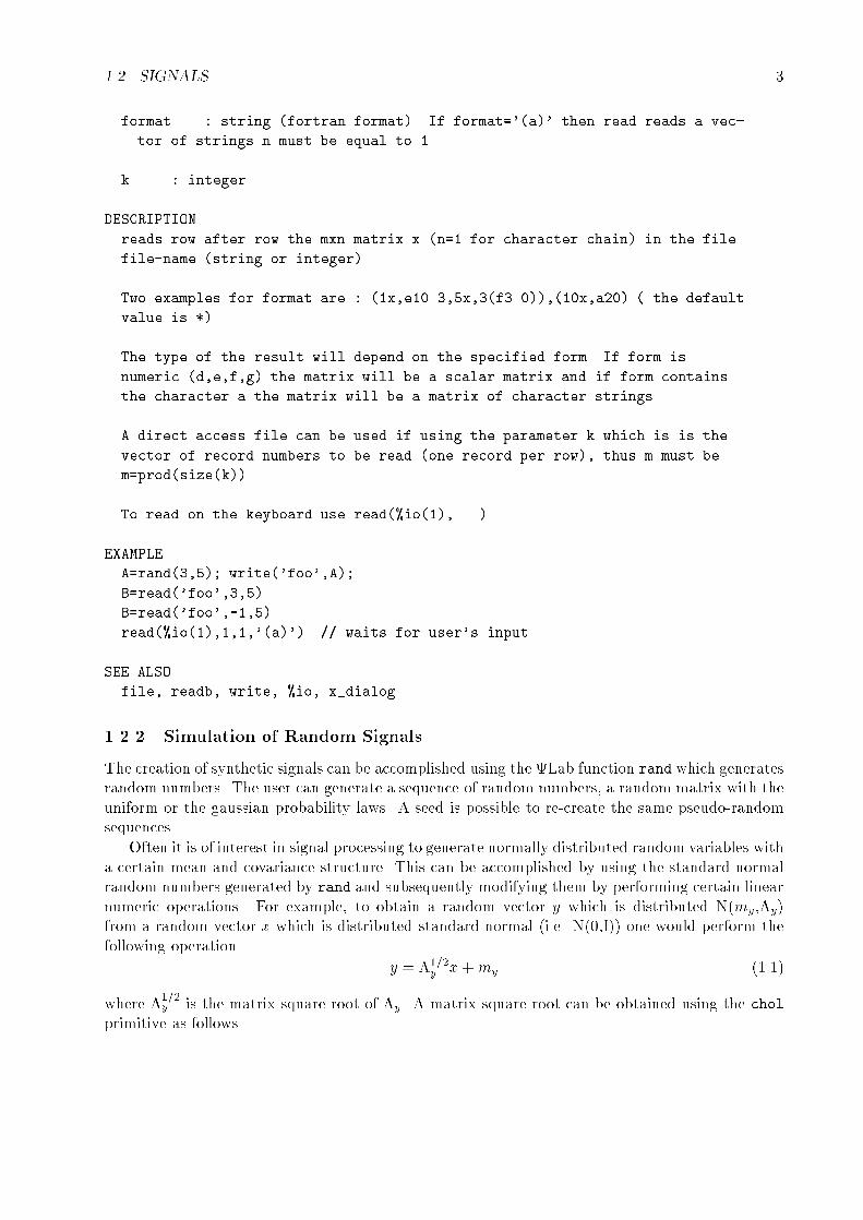
The frequency response of signals and systems requires evaluating the s-transform on the j!-axis or the z-transform on the unit circle. An example of evaluating the magnitude of the frequencyresponse of a continuous-time system is as follows.
-->//Evaluate magnitude response of continuous-time system
-->hs=analpf(4,'cheb1',[.1 0],5)
hs =
161.30794
---------------------------------------------------
2 3 4
179.23104 + 96.905252s + 37.094238s + 4.9181782s + s
-->fr=0:.1:15;
-->hf=freq(hs(2),hs(3),%i*fr);
-->hm=abs(hf);
1.9. PLOTTING SIGNALS 17
1.00 6.40 11.80 17.20 22.60 28.00 33.40 38.80 44.20 49.60 55.00
-0.0924
-0.0732
-0.0539
-0.0347
-0.0154
0.0038
0.0230
0.0423
0.0615
0.0808
0.1000
Figure 1.4: exec('plot1.code') Plot of Filter Impulse Response
-->plot(fr,hm),
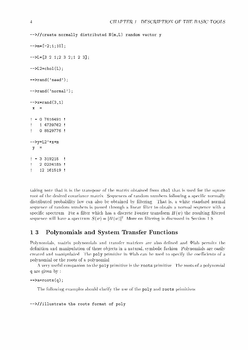
Here we make an analog low-pass �lter using the functions analpf (see Chapter 4 for more details).The �lter is a type I Chebyshev of order 4 where the cut-o� frequency is 5 Hertz. The primitivefreq (see Section 1.3.1) evaluates the transfer function hs at the values of fr on the j!-axis. Theresult is shown in Figure 1.5
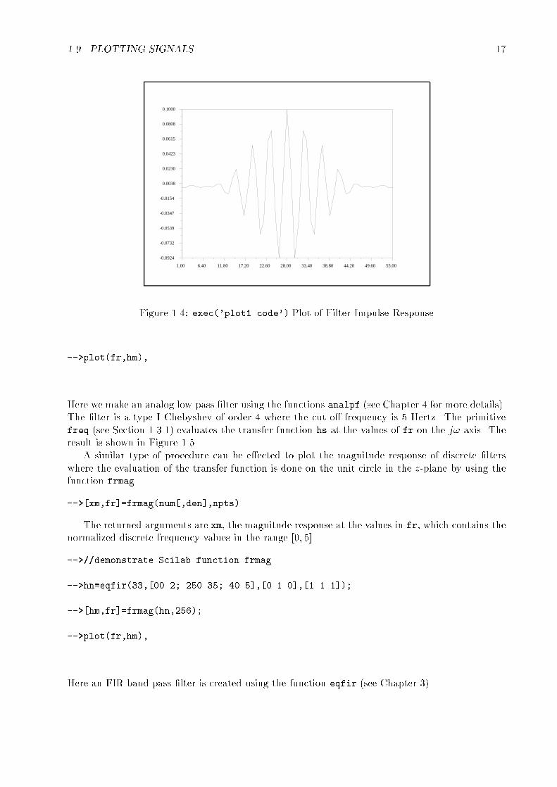
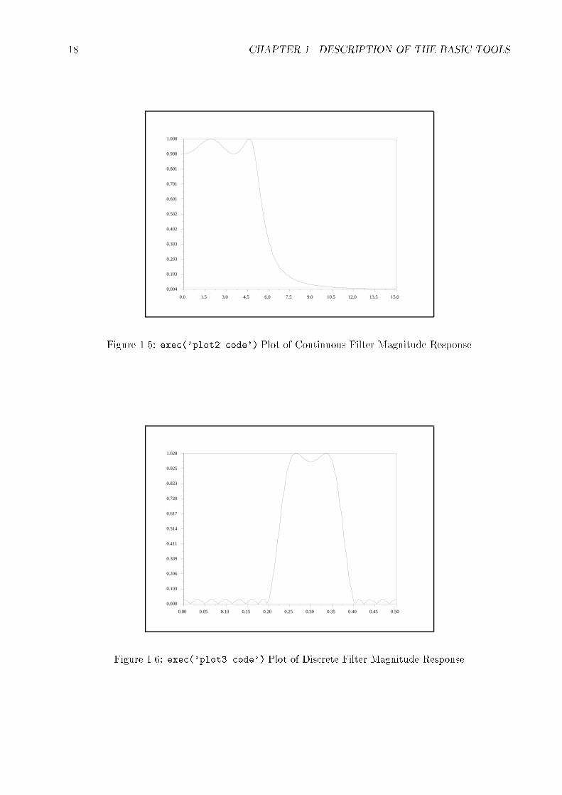
A similar type of procedure can be e�ected to plot the magnitude response of discrete �lterswhere the evaluation of the transfer function is done on the unit circle in the z-plane by using thefunction frmag.
-->[xm,fr]=frmag(num[,den],npts)
The returned arguments are xm, the magnitude response at the values in fr, which contains thenormalized discrete frequency values in the range [0; 5].
-->//demonstrate Scilab function frmag
-->hn=eqfir(33,[00.2;.250.35;.40.5],[0 1 0],[1 1 1]);
-->[hm,fr]=frmag(hn,256);
-->plot(fr,hm),
Here an FIR band-pass �lter is created using the function eqfir (see Chapter 3).
18 CHAPTER 1. DESCRIPTION OF THE BASIC TOOLS
0.0 1.5 3.0 4.5 6.0 7.5 9.0 10.5 12.0 13.5 15.0
0.004
0.103
0.203
0.303
0.402
0.502
0.601
0.701
0.801
0.900
1.000
Figure 1.5: exec('plot2.code') Plot of Continuous Filter Magnitude Response
0.00 0.05 0.10 0.15 0.20 0.25 0.30 0.35 0.40 0.45 0.50
0.000
0.103
0.206
0.309
0.411
0.514
0.617
0.720
0.823
0.925
1.028
Figure 1.6: exec('plot3.code') Plot of Discrete Filter Magnitude Response

1.10. DEVELOPMENT OF SIGNAL PROCESSING TOOLS 19
Other speci�c plotting functions are bode for the Bode plot of rational system transfer functions(see Section 2.1.1), group for the group delay (see Section 2.1.2) and plzr for the poles-zeros plot.
-->//Demonstrate function plzr
-->hz=iir(4,'lp','butt',[.25 0],[0 0])
hz =
2 3 4
0.0939809 + 0.3759234z + 0.5638851z + 0.3759234z + 0.0939809z
-------------------------------------------------------------
2 3 4
0.0176648 + 1.859D-17z + 0.4860288z + 4.163D-17z + z
-->plzr(hz)
Here a third order, low-pass, IIR �lter is created using the function iir (see Section 4.2). Theresulting pole-zero plot is illustrated in Figure 1.7
-1.562 -1.250 -0.938 -0.626 -0.314 -0.002 0.310 0.622 0.934 1.246 1.558
-1.104
-0.884
-0.663
-0.443
-0.223
-0.002
0.218
0.439
0.659
0.880
1.100
ΟΟΟΟ
ZerosΟ-1.562 -1.250 -0.938 -0.626 -0.314 -0.002 0.310 0.622 0.934 1.246 1.558
-1.104
-0.884
-0.663
-0.443
-0.223
-0.002
0.218
0.439
0.659
0.880
1.100
×
×
×
×
Poles×
imag. axis
real axis
transmission zeros and poles
Figure 1.7: exec('plot4.code') Plot of Poles and Zeros of IIR Filter
1.10 Development of Signal Processing Tools
Of course any user can write its own functions like those illustrated in the previous sections. Thesimplest way is to write a �le with a special format . This �le is executed with two Lab primitivesgetf and exec. The complete description of such functionalities is given in the reference manualand the on-line help. These functionalities correspond to the button File Operations.

20 CHAPTER 1. DESCRIPTION OF THE BASIC TOOLS
Chapter 2
Time and Frequency Representation
of Signals
2.1 Frequency Response
2.1.1 Bode Plots
The Bode plot is used to plot the phase and log-magnitude response of functions of a single complexvariable. The log-scale characteristics of the Bode plot permitted a rapid, \back-of-the-envelope"calculation of a system's magnitude and phase response. In the following discussion of Bode plotswe consider only real, causal systems. Consequently, any poles and zeros of the system occur incomplex conjugate pairs (or are strictly real) and the poles are all located in the left-half s-plane.
For H(s) a transfer function of the complex variable s, the log-magnitude of H(s) is de�ned by
M(!) = 20 log10 jH(s)s=j!j (2.1)
and the phase of H(s) is de�ned by
�(!) = tan�1[Im(H(s)s=j!)
Re(H(s)s=j!)] (2.2)
The magnitude, M(!), is plotted on a log-linear scale where the independent axis is marked indecades (sometimes in octaves) of degrees or radians and the dependent axis is marked in decibels.The phase, �(!), is also plotted on a log-linear scale where, again, the independent axis is markedas is the magnitude plot and the dependent axis is marked in degrees (and sometimes radians).
When H(s) is a rational polynomial it can be expressed as
H(s) = C
QNn=1(s� an)QMm=1(s� bm)
(2.3)
where the an and bm are real or complex constants representing the zeros and poles, respectively,of H(s), and C is a real scale factor. For the moment let us assume that the an and bm are strictlyreal. Evaluating (2.3) on the j!-axis we obtain
H(j!) = C
QNn=1(j! � an)QMm=1(j! � bm)
= C
QNn=1
p!2 + a2ne
j tan�1 !=(�an)QMm=1
p!2 + b2me
j tan�1 !=(�bm)(2.4)
21

22 CHAPTER 2. REPRESENTATION OF SIGNALS
and for the log-magnitude and phase response
M(!) =NXn=1
20 logq!2 + a2n �
MXm=1
q!2 + b2m (2.5)
and
�(!) =NXn=1
tan�1(!=(�an))�MXm=1
tan�1(!=(�bm)): (2.6)
To see how the Bode plot is constructed assume that both (2.5) and (2.6) consist of single termscorresponding to a pole of H(s). Consequently, the magnitude and phase become
M(!) = �20 logp!2 + a2 (2.7)
and�(!) = �j tan�1(!=(�a)): (2.8)
We plot the magnitude in (2.7) using two straight line approximations. That is, for j!j � jaj wehave thatM(!) � �20 log jaj which is a constant (i.e., a straight line with zero slope). For j!j � jajwe have that M(!) � �20 log j!j which is a straight line on a log scale which has a slope of -20db/decade. The intersection of these two straight lines is at w = a. Figure 2.1 illustrates these twostraight line approximations for a = 10.
0
101
102
10
-40
-25
-10
Log scale
Figure 2.1: exec('bode1.code') Log-Magnitude Plot of H(s) = 1=(s� a)
When ! = a we have that M(!) = �20 logp2a = �20 log a � 20 logp2. Since 20 log
p2 = 3:0
we have that at ! = a the correction to the straight line approximation is �3db. Figure 2.1illustrates the true magnitude response of H(s) = (s � a)�1 for a = 10 and it can be seen thatthe straight line approximations with the 3db correction at ! = a yields very satisfactory results.The phase in (2.8) can also be approximated. For ! � a we have �(!) � 0 and for ! � a wehave �(!) � �90�. At ! = a we have �(!) = �45�. Figure 2.2 illustrates the straight lineapproximation to �(!) as well as the actual phase response.
2.1. FREQUENCY RESPONSE 23
0
101
102
103
10
-90
-45
0
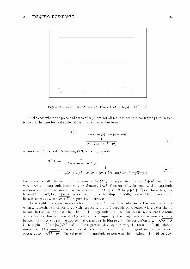
Figure 2.2: exec('bode2.code') Phase Plot of H(s) = 1=(s� a)
In the case where the poles and zeros ofH(s) are not all real but occur in conjugate pairs (whichis always the case for real systems) we must consider the term
H(s) =1
[s� (a+ jb)][s� (a� jb)]
=1
s2 � 2as + (a2 + b2)(2.9)
where a and b are real. Evaluating (2.9) for s = j! yields
H(s) =1
(a2 + b2 � !2)� 2aj!
=1p
!4 + 2(a2 � b2)!2 + (a2 + b2) exp(j tan�1[ �2a!a2+b2�!2 ])
: (2.10)
For ! very small, the magnitude component in (2.10) is approximately 1=(a2 + b2) and for !very large the magnitude becomes approximately 1=!2. Consequently, for small ! the magnituderesponse can be approximated by the straight line M(!) � �20 log10 ja2 + b2j and for ! large wehaveM(!) � �20 log j!2j which is a straight line with a slope of -40db/decade. These two straightlines intersect at ! =
pa2 + b2. Figure 2.3 illustrates
the straight line approximations for a = 10 and b = 25. The behavior of the magnitude plotwhen ! is neither small nor large with respect to a and b depends on whether b is greater than a
or not. In the case where b is less than a, the magnitude plot is similar to the case where the rootsof the transfer function are strictly real, and consequently, the magnitude varies monotonicallybetween the two straight line approximations shown in Figure 2.3. The correction at ! =
pa2 + b2
is -6db plus �20 log ja=(pa2 + b2)j. For b greater than a, however, the term in (2.10) exhibitsresonance. This resonance is manifested as a local maximum of the magnitude response whichoccurs at ! =
pb2 � a2. The value of the magnitude response at this maximum is �20 log j2abj.

24 CHAPTER 2. REPRESENTATION OF SIGNALS
0
101
102
10
-80
-65
-50
Figure 2.3: exec('bode3.code') Log-Magnitude Plot of H(s) = (s2 � 2as+ (a2 + b2))�1
The e�ect of resonance is illustrated in Figure 2.3 as the upper dotted curve. Non-resonant behavioris illustrated in Figure 2.3 by the lower dotted curve.
The phase curve for the expression in (2.10) is approximated as follows. For ! very smallthe imaginary component of (2.10) is small and the real part is non-zero. Thus, the phase isapproximately zero. For ! very large the real part of (2.10) dominates the imaginary part and,consequently, the phase is approximately �180�. At ! =
pa2 + b2 the real part of (2.10) is zero
and the imaginary part is negative so that the phase is exactly �90�. The phase curve is shown inFigure 2.4.
How to Use the Function bode
The description of the transfer function can take two forms: a rational polynomial or a state-spacedescription .
For a transfer function given by a polynomial h the syntax of the call to bode is as follows
-->bode(h,fmin,fmax[,step][,comments])
When using a state-space system representation sl of the transfer function the syntax of thecall to bode is as follows
-->bode(sl,fmin,fmax[,pas][,comments])
where
-->sl=syslin(domain,a,b,c[,d][,x0])
The continuous time state-space system assumes the following form
_x(t) = ax(t) + bu(t)
y(t) = cx(t) + dw(t)

2.1. FREQUENCY RESPONSE 25
0
101
102
103
10
-180
-135
-90
-45
0
Figure 2.4: exec('bode4.code') Phase Plot of H(s) = (s2 � 2as+ (a2 + b2))�1
and x0 is the initial condition. The discrete time system takes the form
x(n+ 1) = ax(n) + bu(n)
y(n) = cx(n) + dw(n)
Examples Using bode
Here are presented examples illustrating the state-space description, the rational polynomial case.These two previous systems connected in series forms the third example.
In the �rst example, the system is de�ned by the state-space description below
_x = �2�x+ u
y = 18�x+ u:
The initial condition is not important since the Bode plot is of the steady state behavior of thesystem.
-->//Bode plot
-->a=-2*%pi;b=1;c=18*%pi;d=1;
-->sl=syslin('c',a,b,c,d);
-->bode(sl,.1,100);
The result of the call to bode for this example is illustrated in Figure 2.5.The following example illustrates the use of the bode function when the user has an explicit
rational polynomial representation of the system.

26 CHAPTER 2. REPRESENTATION OF SIGNALS
-1
100
101
102
10
0
5
10
15
20 db
Hz
Magnitude
-1
100
101
102
10
-90
0 degrees
Hz
Phase
Figure 2.5: exec('bode5.code') Bode Plot of State-Space System Representation
-->//Bode plot; rational polynomial
-->s=poly(0,'s');
-->h1=1/real((s+2*%pi*(15+100*%i))*(s+2*%pi*(15-100*%i)))
h1 =
1
-------------------------
2
403666.82 + 188.49556s + s
-->h1=syslin('c',h1);
-->bode(h1,10,1000,.01);
The result of the call to bode for this example is illustrated in Figure 2.6.
The �nal example combines the systems used in the two previous examples by attaching themtogether in series. The state-space description is converted to a rational polynomial descriptionusing the ss2tf function.
-->//Bode plot; two systems in series
-->a=-2*%pi;b=1;c=18*%pi;d=1;
-->sl=syslin('c',a,b,c,d);
2.1. FREQUENCY RESPONSE 27
0
101
102
103
10
-160
-150
-140
-130
-120
-110
-100 db
Hz
Magnitude
0
101
102
103
10
-180
-90
0 degrees
Hz
Phase
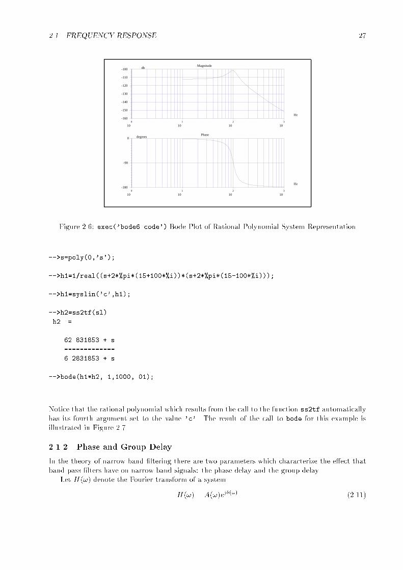
Figure 2.6: exec('bode6.code') Bode Plot of Rational Polynomial System Representation
-->s=poly(0,'s');
-->h1=1/real((s+2*%pi*(15+100*%i))*(s+2*%pi*(15-100*%i)));
-->h1=syslin('c',h1);
-->h2=ss2tf(sl)
h2 =
62.831853 + s
-------------
6.2831853 + s
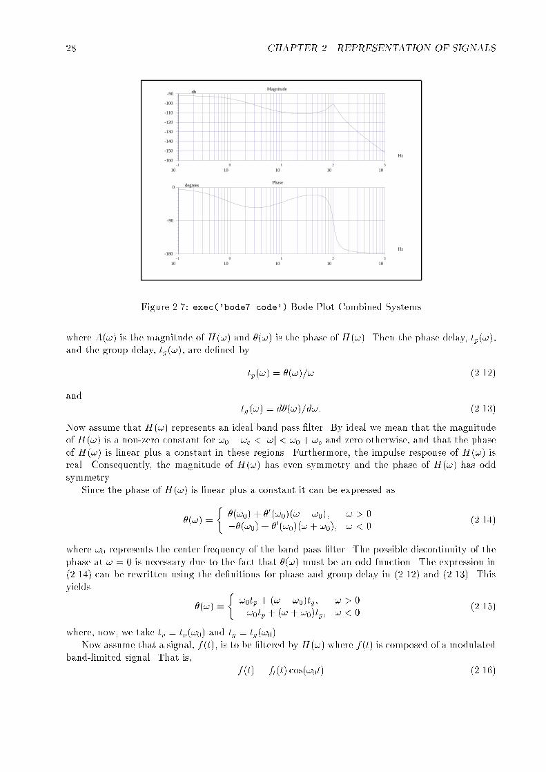
-->bode(h1*h2,.1,1000,.01);
Notice that the rational polynomial which results from the call to the function ss2tf automaticallyhas its fourth argument set to the value 'c'. The result of the call to bode for this example isillustrated in Figure 2.7.
2.1.2 Phase and Group Delay
In the theory of narrow band �ltering there are two parameters which characterize the e�ect thatband pass �lters have on narrow band signals: the phase delay and the group delay.
Let H(!) denote the Fourier transform of a system
H(!) = A(!)ej�(!) (2.11)
28 CHAPTER 2. REPRESENTATION OF SIGNALS
-1
100
101
102
103
10
-160
-150
-140
-130
-120
-110
-100
-90 db
Hz
Magnitude
-1
100
101
102
103
10
-180
-90
0 degrees
Hz
Phase
Figure 2.7: exec('bode7.code') Bode Plot Combined Systems
where A(!) is the magnitude of H(!) and �(!) is the phase of H(!). Then the phase delay, tp(!),and the group delay, tg(!), are de�ned by
tp(!) = �(!)=! (2.12)
and
tg(!) = d�(!)=d!: (2.13)
Now assume that H(!) represents an ideal band pass �lter. By ideal we mean that the magnitudeof H(!) is a non-zero constant for !0 � !c < j!j < !0 + !c and zero otherwise, and that the phaseof H(!) is linear plus a constant in these regions. Furthermore, the impulse response of H(!) isreal. Consequently, the magnitude of H(!) has even symmetry and the phase of H(!) has oddsymmetry.
Since the phase of H(!) is linear plus a constant it can be expressed as
�(!) =
(�(!0) + �0(!0)(! � !0); ! > 0��(!0) + �0(!0)(! + !0); ! < 0
(2.14)
where !0 represents the center frequency of the band pass �lter. The possible discontinuity of thephase at ! = 0 is necessary due to the fact that �(!) must be an odd function. The expression in(2.14) can be rewritten using the de�nitions for phase and group delay in (2.12) and (2.13). Thisyields
�(!) =
(!0tp + (! � !0)tg; ! > 0�!0tp + (! + !0)tg; ! < 0
(2.15)
where, now, we take tp = tp(!0) and tg = tg(!0).Now assume that a signal, f(t), is to be �ltered by H(!) where f(t) is composed of a modulated
band-limited signal. That is,
f(t) = fl(t) cos(!0t) (2.16)
2.1. FREQUENCY RESPONSE 29
where !0 is the center frequency of the band pass �lter and Fl(!) is the Fourier transform a thebandlimited signal fl(t) (Fl(!) = 0 for j!j > !c). It is now shown that the output of the �lter dueto the input in (2.16) takes the following form
g(t) = fl(t+ tg) cos[!0(t+ tp)]: (2.17)
To demonstrate the validity of (2.17) the Fourier transform of the input in (2.16) is written as
F (!) =1
2[Fl(! � !0) + Fl(! + !0)] (2.18)
where (2.18) represents the convolution of Fl(!) with the Fourier transform of cos(!0t). The Fouriertransform of the �lter, H(!), can be written
H(!) =
8><>:
e!0tp+(!�!0)tg ; !0 � !c < ! < !0 + !ce�!0tp+(!+!0)tg ; �!0 � !c < ! < �!0 + !c0; otherwise
(2.19)
Thus, since G(!) = F (!)H(!),
G(!) =
(12Fl(! � !0)e!0tp+(!�!0)tg ; !0 � !c < ! < !0 + !c12Fl(! + !0)e
�!0tp+(!+!0)tg ; �!0 � !c < ! < �!0 + !c(2.20)
Calculating g(t) using the inverse Fourier transform
g(t) =1
2�
Z1
�1
F (!)H(!)
=1
2
1
2�[
Z !0+!c
!0�!cFl(! � !0)e
j[(!�!0)tg+!0tp]ej!td!
+
Z�!0+!c
�!0�!cFl(! + !0)e
j[(!+!0)tg�!0tp]ej!td!] (2.21)
Making the change in variables u = ! � !0 and v = ! + !0yields
g(t) =1
2
1
2�[
Z !c
�!cFl(u)e
j[utg+!0tp]ejutej!0tdu
+Z !c
�!cFl(v)e
j[vtg�!0tp]ejvte�j!0tdv] (2.22)
Combining the integrals and performing some algebra gives
g(t) =1
2
1
2�
Z !c
�!cFl(!)e
j!tgej!t[ej!0tpej!0t + e�j!0tpe�j!0t]d!
=1
2�
Z !c
�!cFl(!) cos[!0(t+ tp)]e
j!(t+tg)d!
= cos[!0(t+ tp)]1
2�
Z !c
�!cFl(!)e
j!(t+tg)d!
= cos[!0(t+ tp)]fl(t+ tg) (2.23)
which is the desired result.The signi�cance of the result in (2.23) is clear. The shape of the signal envelope due to fl(t)
is unchanged and shifted in time by tg . The carrier, however, is shifted in time by tp (which in

30 CHAPTER 2. REPRESENTATION OF SIGNALS
1.00 6.40 11.80 17.20 22.60 28.00 33.40 38.80 44.20 49.60 55.00
-1.0
-0.8
-0.6
-0.4
-0.2
0.0
0.2
0.4
0.6
0.8
1.0
Figure 2.8: exec('group1 5.code') Modulated Exponential Signal
general is not equal to tg). Consequently, the overall appearance of the ouput signal is changedwith respect to that of the input due to the di�erence in phase shift between the carrier and theenvelope. This phenomenon is illustrated in Figures 2.8-2.12. Figure 2.8 illustrates
a narrowband signal which consists of a sinusoid modulated by an envelope. The envelope isan decaying exponential and is displayed in the �gure as the dotted curve.
Figure 2.9 shows the band pass �lter used to �lter the signal in Figure 2.8. The �lter magnitudeis plotted as the solid curve and the �lter phase is plotted as the dotted curve.
Notice that since the phase is a constant function that tg = 0. The value of the phase delay istp = �=2. As is expected, the �ltered output of the �lter consists of the same signal as the inputexcept that the sinusoidal carrier is now phase shifted by �=2. This output signal is displayed inFigure 2.10 as the solid curve. For reference the input signal is plotted as the dotted curve.
To illustrate the e�ect of the group delay on the �ltering process a new �lter is constructed asis displayed in Figure 2.11.
Here the phase is again displayed as the dotted curve. The group delay is the slope of the phasecurve as it passes through zero in the pass band region of the �lter. Here tg = �1 and tp = 0.The result of �ltering with this phase curve is display in Figure 2.12. As expected, the envelope isshifted but the sinusoid is not shifted within the reference frame of the window. The original inputsignal is again plotted as the dotted curve for reference.
The Function group
As can be seen from the explanation given in this section, it is preferable that the group delay ofa �lter be constant. A non-constant group delay tends to cause signal deformation. This is dueto the fact that the di�erent frequencies which compose the signal are time shifted by di�erentamounts according to the value of the group delay at that frequency. Consequently, it is valuableto examine the group delay of �lters during the design procedure. The function group accepts �lterparameters in several formats as input and returns the group delay as output. The syntax of thefunction is as follows:

2.1. FREQUENCY RESPONSE 31
1.00 6.40 11.80 17.20 22.60 28.00 33.40 38.80 44.20 49.60 55.00
-4.0
-3.2
-2.4
-1.6
-0.8
0.0
0.8
1.6
2.4
3.2
4.0
Figure 2.9: exec('group1 5.code') Constant Phase Band Pass Filter
1.00 6.40 11.80 17.20 22.60 28.00 33.40 38.80 44.20 49.60 55.00
-1.0
-0.8
-0.6
-0.4
-0.2
0.0
0.2
0.4
0.6
0.8
1.0
Figure 2.10: exec('group1 5.code') Carrier Phase Shift by tp = �=2

32 CHAPTER 2. REPRESENTATION OF SIGNALS
1.00 6.40 11.80 17.20 22.60 28.00 33.40 38.80 44.20 49.60 55.00
-15
-12
-9
-6
-3
0
3
6
9
12
15
Figure 2.11: exec('group1 5.code') Linear Phase Band Pass Filter
1.00 6.40 11.80 17.20 22.60 28.00 33.40 38.80 44.20 49.60 55.00
-1.0
-0.8
-0.6
-0.4
-0.2
0.0
0.2
0.4
0.6
0.8
1.0
Figure 2.12: exec('group1 5.code') Envelope Phase Shift by tg = �1

2.1. FREQUENCY RESPONSE 33
-->[tg,fr]=group(npts,h)
The group delay tg is evaluated in the interval [0,.5) at equally spaced samples contained in fr. Thenumber of samples is governed by npts. Three formats can be used for the speci�cation of the �lter.The �lter h can be speci�ed by a vector of real numbers, by a rational polynomial representing thez-transform of the �lter, or by a matrix polynomial representing a cascade decomposition of the�lter. The three cases are illustrated below.
The �rst example is for a linear-phase �lter designed using the function wfir
-->[h w]=wfir('lp',7,[.2,0],'hm',[0.01,-1]);
-->h'
ans =
! - 0.0049893 !
! 0.0290002 !
! 0.2331026 !
! 0.4 !
! 0.2331026 !
! 0.0290002 !
! - 0.0049893 !
-->[tg,fr]=group(100,h);
-->plot2d(fr',tg',1,'011',' ',[0,2,0.5,4.])
as can be seen in Figure 2.13the group delay is a constant, as is to be expected for a linear phase �lter. The second example
speci�es a rational polynomial for the �lter transfer function:
-->z=poly(0,'z');
-->h=z/(z-0.5)
h =
z
-------
- 0.5 + z
-->[tg,fr]=group(100,h);
-->plot(fr,tg)
The plot in Figure 2.14 gives the result of this calculation.Finally, the third example gives the transfer function of the �lter in cascade form.

34 CHAPTER 2. REPRESENTATION OF SIGNALS
0.00 0.05 0.10 0.15 0.20 0.25 0.30 0.35 0.40 0.45 0.50
2.0
2.2
2.4
2.6
2.8
3.0
3.2
3.4
3.6
3.8
4.0
++++++++++++++++++++++++++++++++++++++++++++++++++++++++++++++++++++++++++++++++++++++++++++++++++++
Figure 2.13: exec('group6 8.code') Group Delay of Linear-Phase Filter
0.0000 0.0495 0.0990 0.1485 0.1980 0.2475 0.2970 0.3465 0.3960 0.4455 0.4950
-0.333
-0.200
-0.067
0.067
0.200
0.333
0.467
0.600
0.733
0.867
1.000
Figure 2.14: exec('group6 8.code') Group Delay of Filter (Rational Polynomial)

2.1. FREQUENCY RESPONSE 35
-->h=[1 1.5 -1 1;2 -2.5 -1.7 0;3 3.5 2 5]';
--> cels=[];
--> for col=h,
nf=[col(1:2);1];
nd=[col(3:4);1];
cels=[cels,list('r',poly(nf,'z','c'),poly(nd,'z','c'),[])];
end,
Warning : use of standard list to define typed structures
is obsolete. Use tlist
-->[tg,fr]=group(100,cels);
-->//plot(fr,tg)
The result is shown in Figure 2.15. The cascade realization is known for numerical stability.
0.0000 0.0495 0.0990 0.1485 0.1980 0.2475 0.2970 0.3465 0.3960 0.4455 0.4950
-1.133
-0.680
-0.226
0.228
0.682
1.136
1.590
2.044
2.497
2.951
3.405
Figure 2.15: exec('group6 8.code') Group Delay of Filter (Cascade Realization)
2.1.3 Appendix: Lab Code Used to Generate Examples
The following listing of Lab code was used to generate the examples of the this section.
//exec('group1_5.code')
//create carrier and narrow band signal

36 CHAPTER 2. REPRESENTATION OF SIGNALS
xinit('group1.ps');
wc=1/4;
x=sin(2*%pi*(0:54)*wc);
y=exp(-abs(-27:27)/5);
f=x.*y;
plot([1 1 55],[1 -1 -1]),
nn=prod(size(f))
plot2d((1:nn)',f',[-2],"000"),
nn=prod(size(y))
plot2d((1:nn)',y',[-3],"000"),
plot2d((1:nn)',-y',[-3],"000"),
xend(),
xinit('group2.ps');
//make band pass filter
[h w]=wfir('bp',55,[maxi([wc-.15,0]),mini([wc+.15,.5])],'kr',60.);
//create new phase function with only phase delay
hf=fft(h,-1);
hm=abs(hf);
hp=%pi*ones(1:28);//tg is zero
hp(29:55)=-hp(28:-1:2);
hr=hm.*cos(hp);
hi=hm.*sin(hp);
hn=hr+%i*hi;
plot([1 1 55],[4 -4 -4]),
plot2d([1 55]',[0 0]',[-1],"000"),
nn=prod(size(hp))
plot2d((1:nn)',hp',[-2],"000"),
nn=prod(size(hm))
plot2d((1:nn)',2.5*hm',[-1],"000"),
xend(),
xinit('group3.ps');
//filter signal with band pass filter
ff=fft(f,-1);
gf=hn.*ff;
g=fft(gf,1);
plot([1 1 55],[1 -1 -1]),
nn=prod(size(g))
plot2d((1:nn)',real(g)',[-2],"000"),
nn=prod(size(f))
plot2d((1:nn)',f',[-1],"000"),
xend(),
//create new phase function with only group delay

2.2. SAMPLING 37
xinit('group4.ps');
tg=-1;
hp=tg*(0:27)-tg*12.*ones(1:28)/abs(tg);//tp is zero
hp(29:55)=-hp(28:-1:2);
hr=hm.*cos(hp);
hi=hm.*sin(hp);
hn=hr+%i*hi;
plot([1 1 55],[15 -15 -15]),
plot2d([1 55]',[0 0]',[-1],"000"),
nn=prod(size(hp))
plot2d((1:nn)',hp',[-2],"000"),
nn=prod(size(hm))
plot2d((1:nn)',10*hm',[-1],"000"),
xend(),
xinit('group5.ps');
//filter signal with band pass filter
ff=fft(f,-1);
gf=hn.*ff;
g=fft(gf,1);
plot([1 1 55],[1 -1 -1]),
nn=prod(size(g))
plot2d((1:nn)',real(g)',[-2],"000"),
nn=prod(size(f))
plot2d((1:nn)',f',[-1],"000"),
xend(),
2.2 Sampling
The remainder of this section explains in detail the relationship between continuous and discretesignals.
To begin, it is useful to examine the Fourier transform pairs for continuous and discrete timesignals. For x(t) and X() a continuous time signal and its Fourier transform, respectively, wehave that
X() =
Z1
�1
x(t)e�jtdt (2.24)
x(t) =1
2�
Z1
�1
X()ejtd: (2.25)
For x(n) and X(!) a discrete time signal and its Fourier transform, respectively, we have that
X(!) =1X
n=�1
x(n)e�j!n (2.26)
x(n) =1
2�
Z �
��X(!)ej!nd!: (2.27)
38 CHAPTER 2. REPRESENTATION OF SIGNALS
The discrete time signal, x(n), is obtained by sampling the continuous time signal, x(t), at regularintervals of length T called the sampling period. That is,
x(n) = x(t)jt=nT (2.28)
We now derive the relationship between the Fourier transforms of the continuous and discrete timesignals. The discussion follows [21].
Using (2.28) in (2.25) we have that
x(n) =1
2�
Z1
�1
X()ejnTd: (2.29)
Rewriting the integral in (2.29) as a sum of integrals over intervals of length 2�=T we have that
x(n) =1
2�
1Xr=�1
Z (2�r+�)=T
(2�r��)=TX()ejnTd (2.30)
or, by a change of variables
x(n) =1
2�
1Xr=�1
Z �=T
��=TX(+
2�r
T)ejnT ej2�nrd: (2.31)
Interchanging the sum and the integral in (2.31) and noting that ej2�nr = 1 due to the fact that nand r are always integers yields
x(n) =1
2�
Z �=T
��=T[
1Xr=�1
X(+2�r
T)]ejnTd: (2.32)
Finally, the change of variables ! = T gives
x(n) =1
2�
Z �
��[1
T
1Xr=�1
X(!
T+
2�r
T)]ej!nd! (2.33)
which is identical in form to (2.27). Consequently, the following relationship exists between theFourier transforms of the continuous and discrete time signals:
X(!) =1
T
1Xr=�1
X(!
T+2�r
T)
=1
T
1Xr=�1
X(+2�r
T): (2.34)
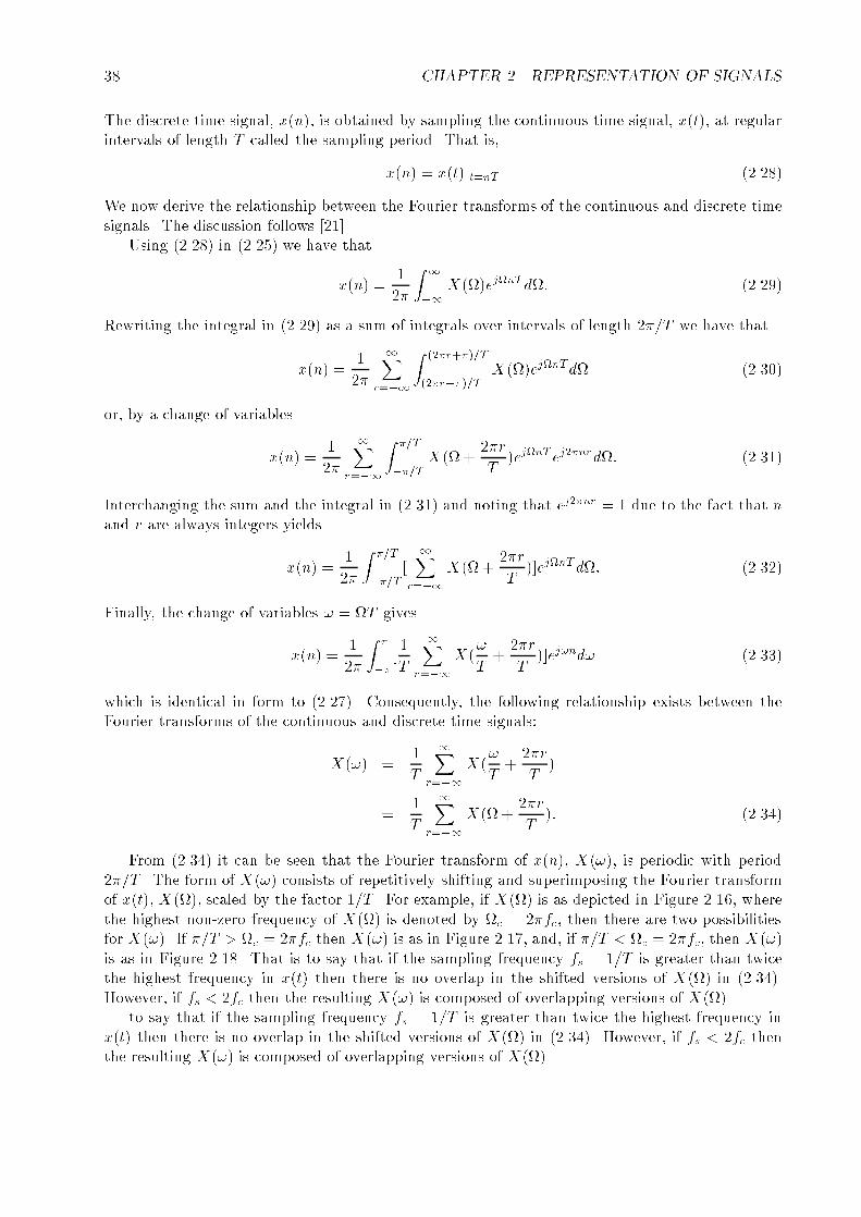
From (2.34) it can be seen that the Fourier transform of x(n), X(!), is periodic with period2�=T . The form of X(!) consists of repetitively shifting and superimposing the Fourier transformof x(t), X(), scaled by the factor 1=T . For example, if X() is as depicted in Figure 2.16, wherethe highest non-zero frequency of X() is denoted by c = 2�fc, then there are two possibilitiesfor X(!). If �=T > c = 2�fc then X(!) is as in Figure 2.17, and, if �=T < c = 2�fc, then X(!)is as in Figure 2.18. That is to say that if the sampling frequency fs = 1=T is greater than twicethe highest frequency in x(t) then there is no overlap in the shifted versions of X() in (2.34).However, if fs < 2fc then the resulting X(!) is composed of overlapping versions of X().
to say that if the sampling frequency fs = 1=T is greater than twice the highest frequency inx(t) then there is no overlap in the shifted versions of X() in (2.34). However, if fs < 2fc thenthe resulting X(!) is composed of overlapping versions of X().

2.2. SAMPLING 39
-5 -4 -3 -2 -1 0 1 2 3 4 5
-2.0
-1.3
-0.6
0.1
0.8
1.5
2.2
2.9
3.6
4.3
5.0
Wc -Wc
X(W)
W
X(0)
Figure 2.16: exec('sample1.code') Frequency Response X()
-5 -4 -3 -2 -1 0 1 2 3 4 5
-2.0
-1.3
-0.6
0.1
0.8
1.5
2.2
2.9
3.6
4.3
5.0
pi/T
X(W)
W
X(0)/T
Figure 2.17: exec('sample2.code') Frequency Response x(!) With No Aliasing
40 CHAPTER 2. REPRESENTATION OF SIGNALS
-5 -4 -3 -2 -1 0 1 2 3 4 5
-2.0
-1.3
-0.6
0.1
0.8
1.5
2.2
2.9
3.6
4.3
5.0
pi/T
X(W)
W
X(0)/T
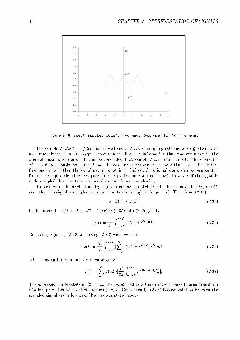
Figure 2.18: exec('sample3.code') Frequency Response x(!) With Aliasing
The sampling rate T = 1=(2fc) is the well known Nyquist sampling rate and any signal sampledat a rate higher than the Nyquist rate retains all of the information that was contained in theoriginal unsampled signal. It can be concluded that sampling can retain or alter the characterof the original continuous time signal. If sampling is performed at more than twice the highestfrequency in x(t) then the signal nature is retained. Indeed, the original signal can be recuperatedfrom the sampled signal by low pass �ltering (as is demonstrated below). However, if the signal isundersampled this results in a signal distortion known as aliasing.
To recuperate the original analog signal from the sampled signal it is assumed that c < �=T(i.e., that the signal is sampled at more than twice its highest frequency). Then from (2.34)
X() = TX(!) (2.35)
in the interval ��=T � � �=T . Plugging (2.35) into (2.25) yields
x(t) =1
2�
Z �=T
��=TTX(!)ejtd: (2.36)
Replacing X(!) by (2.26) and using (2.28) we have that
x(t) =T
2�
Z �=T
��=T[1X�1
x(nT )e�jnT ]ejtd: (2.37)
Interchanging the sum and the integral gives
x(t) =1X�1
x(nT )[T
2�
Z �=T
��=Tej(t�nT )d]: (2.38)
The expression in brackets in (2.38) can be recognized as a time shifted inverse Fourier transformof a low pass �lter with cut-o� frequency �=T . Consequently, (2.38) is a convolution between thesampled signal and a low pass �lter, as was stated above.

2.3. DECIMATION AND INTERPOLATION 41
We now illustrate the e�ects of aliasing. Since square integrable functions can always be de-composed as a sum of sinusoids the discussion is limited to a signal which is a cosine function. Theresults of what happens to a cosine signal when it is undersampled is directly extensible to morecomplicated signals.
We begin with a cosine signal as is illustrated in Figure 2.19.
0 500 1000 1500 2000 2500 3000 3500 4000 4500 5000
-1.5
-1.2
-0.9
-0.6
-0.3
0.0
0.3
0.6
0.9
1.2
1.5
Figure 2.19: exec('sample4.code') Cosine Signal
The cosine in Figure 2.19 is actually a sampled signal which consists of 5000 samples. Oneperiod of the cosine in the �gure is 200 samples long, consequently, the Nyquist sampling raterequires that we retain one sample in every 100 to retain the character of the signal. By samplingthe signal at a rate less than the Nyquist rate it would be expected that aliasing would occur.That is, it would be expected that the sum of two cosines would be evident in the resampled data.Figure 2.20 illustrates the data resulting from sampling the cosine in Figure 2.19 at a rate of onesevery 105 samples.
As can be seen in Figure 2.20, the signal is now the sum of two cosines which is illustrated bythe beat signal illustrated by the dotted curves.
2.3 Decimation and Interpolation
2.3.1 Introduction
There often arises a need to change the sampling rate of a digital signal. The Fourier transform of acontinuous-time signal, x(t), and the Fourier transform of the discrete-time signal, x(nT ), obtainedby sampling x(t) with frequency 1=T . are de�ned, respectively, in (2.39) and (2.40) below
X̂(!) =Z1
�1
x(t)e�j!tdt (2.39)
X(ej!T) =1X
n=�1
x(nT )e�j!T : (2.40)
42 CHAPTER 2. REPRESENTATION OF SIGNALS
0.0 4.8 9.6 14.4 19.2 24.0 28.8 33.6 38.4 43.2 48.0
-1.5
-1.2
-0.9
-0.6
-0.3
0.0
0.3
0.6
0.9
1.2
1.5
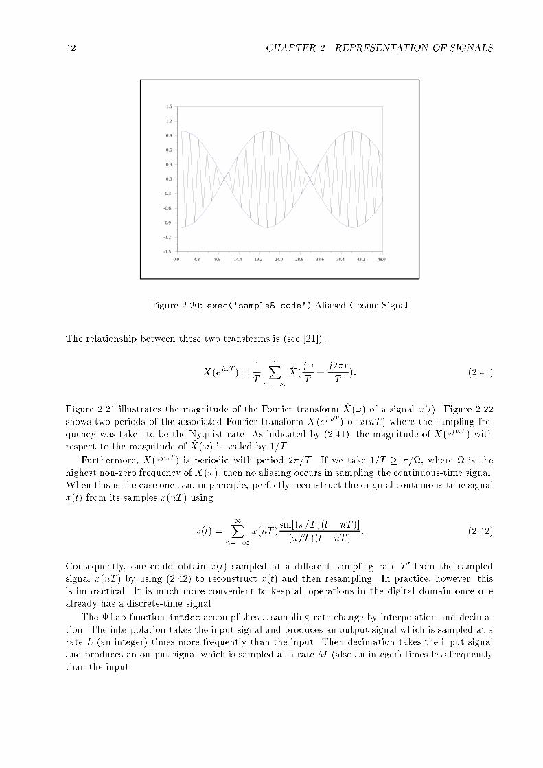
Figure 2.20: exec('sample5.code') Aliased Cosine Signal
The relationship between these two transforms is (see [21]) :
X(ej!T ) =1
T
1Xr=�1
X̂(j!
T+j2�r
T): (2.41)
Figure 2.21 illustrates the magnitude of the Fourier transform X̂(!) of a signal x(t). Figure 2.22shows two periods of the associated Fourier transform X(ejwT ) of x(nT ) where the sampling fre-quency was taken to be the Nyquist rate. As indicated by (2.41), the magnitude of X(ejwT ) withrespect to the magnitude of X̂(!) is scaled by 1=T .
Furthermore, X(ejwT ) is periodic with period 2�=T . If we take 1=T � �=, where is thehighest non-zero frequency of X(!), then no aliasing occurs in sampling the continuous-time signal.When this is the case one can, in principle, perfectly reconstruct the original continuous-time signalx(t) from its samples x(nT ) using
x(t) =1X
n=�1
x(nT )sin[(�=T )(t� nT )]
(�=T )(t� nT ): (2.42)
Consequently, one could obtain x(t) sampled at a di�erent sampling rate T 0 from the sampledsignal x(nT ) by using (2.42) to reconstruct x(t) and then resampling. In practice, however, thisis impractical. It is much more convenient to keep all operations in the digital domain once onealready has a discrete-time signal.
The Lab function intdec accomplishes a sampling rate change by interpolation and decima-tion. The interpolation takes the input signal and produces an output signal which is sampled at arate L (an integer) times more frequently than the input. Then decimation takes the input signaland produces an output signal which is sampled at a rateM (also an integer) times less frequentlythan the input.

2.3. DECIMATION AND INTERPOLATION 43
-60 -48 -36 -24 -12 0 12 24 36 48 60
0.0
0.1
0.2
0.3
0.4
0.5
0.6
0.7
0.8
0.9
1.0
Figure 2.21: exec('intdec1 4.code') Fourier Transform of a Continuous Time Signal
-6.28 -5.03 -3.77 -2.51 -1.26 0.00 1.26 2.51 3.77 5.03 6.28
0.0
0.1
0.2
0.3
0.4
0.5
0.6
0.7
0.8
0.9
1.0
Figure 2.22: exec('intdec1 4.code') Fourier Transform of the Discrete Time Signal

44 CHAPTER 2. REPRESENTATION OF SIGNALS
2.3.2 Interpolation
In interpolating the input signal by the integer L we wish to obtain a new signal x(nT 0) wherex(nT 0) would be the signal obtained if we had originally sampled the continuous-time signal x(t)at the rate 1=T 0 = L=T . If the original signal is bandlimited and the sampling rate f = 1=T isgreater than twice the highest frequency of x(t) then it can be expected that the new sampledsignal x(nT 0) (sampled at a rate of f 0 = 1=T 0 = L=T = Lf) could be obtained directly from thediscrete signal x(nT ).
An interpolation of x(nT ) to x(nT 0) where T 0 = T=L can be found by inserting L � 1 zerosbetween each element of the sequence x(nT ) and then low pass �ltering. To see this we constructthe new sequence v(nT 0) by putting L� 1 zeros between the elements of x(nT )
v(nT 0) =
(x(nT=L); n = 0;�L;�2L; : : :0; otherwise:
(2.43)
Since T 0 = T=L, v(nT 0) is sampled L times more frequently than x(nT ). The Fourier transform of(2.43) yields
V (ej!T0
) =1X
n=�1
v(nT 0)e�j!nT0
=1X
n=�1
x(nT )e�j!nLT0
=1X
n=�1
x(nT )e�j!nT
= X(ej!T ): (2.44)
From (2.44) it can be seen that V (ej!T0
) is periodic with period 2�=T and, also, period 2�=T 0 =2�L=T . This fact is illustrated in Figure 2.23 where L = 3. Since the sampling frequency of V is1=T 0 we see that by �ltering v(nT 0) with a low
pass �lter with cut-o� frequency at �=T we obtain exactly the interpolated sequence, x(nT 0),which we seek (see Figure 2.24), except for a scale factor of L (see (2.41)).
2.3.3 Decimation
Where the object of interpolation is to obtain x(nT 0) from x(nT ) where T 0 = L=T , the object ofdecimation is to �nd x(nT 00) from x(nT ) where T 00 = MT , M an integer. That is, x(nT 00) shouldbe equivalent to a sequence obtained by sampling x(t)M times less frequently than that for x(nT ).Obviously this can be accomplished by keeping only every M th sample of x(nT ). However, if thesampling frequency 1=T is close to the Nyquist rate then keeping only every M th sample resultsin aliasing. Consequently, low pass �ltering the sequence x(nT ) before discarding M � 1 of eachM points is advisable. Assuming that the signal x(nT ) is sampled at the Nyquist rate, the cut-o�frequency of the low pass �lter must be at �=(MT ).
2.3.4 Interpolation and Decimation
To change the sampling rate of a signal by a non-integer quantity it su�ces to perform a combinationof the interpolation and decimation operations. Since both operations use a low-pass �lter they canbe combined as illustrated in the block diagram of Figure 2.25. The Lab function intdec beginsby designing a low-pass �lter for the diagram illustrated in the �gure. It accomplishes this by using

2.3. DECIMATION AND INTERPOLATION 45
-18.85 -15.08 -11.31 -7.54 -3.77 0.00 3.77 7.54 11.31 15.08 18.85
0.0
0.3
0.6
0.9
1.2
1.5
1.8
2.1
2.4
2.7
3.0
Figure 2.23: exec('intdec1 4.code') Fourier Transform of v(nT 0)
-6.28 -5.03 -3.77 -2.51 -1.26 0.00 1.26 2.51 3.77 5.03 6.28
0.0
0.1
0.2
0.3
0.4
0.5
0.6
0.7
0.8
0.9
1.0
Figure 2.24: exec('intdec1 4.code') Fourier Transform of x(nT 0)

46 CHAPTER 2. REPRESENTATION OF SIGNALS
x(nT )-Put
L-1 ZerosBetween
Each Sample
- LPF -Discard
M-1 of EveryM Samples
- x(nMT=L)
Figure 2.25: Block Diagram of Interpolation and Decimation
the wfir �lter design function. This is followed by taking the Fourier transform of both the inputsignal and the low-pass �lter (whose magnitude is �rst scaled by L) by using the fft function.Care must be taken to obtain a linear convolution between the two sequences by adding on anappropriate number of zeros to each sequence before the FFT is performed. After multiplying thetwo transformed sequences together an inverse Fourier transform is performed. Finally, the outputis obtained by discarding M � 1 of each M points. The cut-o� frequency of the low pass �lter is�=T if L > M and is (L�)=(MT ) if L < M .
The practical implementation of the interpolation and decimation procedure is as follows. Ifthe length of the input is N then after putting L� 1 zeros between each element of x the resultingsequence will be of length (N�1)L+1. This new sequence is then lengthened by K�1 zeros whereK is the length of the low pass �lter. This lengthening is to obtain a linear convolution betweenthe input and the low pass �lter with the use of the FFT. The cut-o� frequency of the low pass�lter is chosen to be (:5N)=[(N � 1)L+K] if L > M and (:5NL)=(M [(N � 1)L+K]) if L < M .The FFT's of the two modi�ed sequences are multiplied element by element and then are inverseFourier transformed. The resulting sequence is of length (N � 1)L+ K. To obtain a sequence oflength of (N � 1)L+ 1 elements, (K � 1)=2 elements are discarded o� of each end. Finally, M � 1out of every M elements are discarded to form the output sequence.
2.3.5 Examples using intdec
Here we take a 50-point sequence assumed to be sampled at a 10kHz rate and change it to asequence sampled at 16kHz. Under these conditions we take L = 8 and M = 5. The sequence,x(nT ), is illustrated in Figure 2.26. The discrete Fourier transform of x(nT) is shown in
Figure 2.27. As can be seen, x(nT ) is a bandlimited sequence. A new sequence v(nT 0) is createdby putting 7 zeros between each element of x(nT ). We use a Hamming windowed lowpass �lter oflength 33 (Figure 2.28)
to �lter v(nT 0). The discrete Fourier transform of v(nT 0) is illustrated in Figure 2.29. As is tobe expected, the Fourier transform of v(nT 0) looks like the Fourier transform of x(nT ) repeated 8times.
The result of multiplying the magnitude response of the �lter with that of the sequence v(nT 0)is shown in Figure 2.30. Since the low pass �lter is not ideal the resulting �ltered sequence hassome additional high frequency energy in it (i.e., the small lobes seen in Figure 2.30).
Finally, after taking the inverse discrete Fourier transform and discarding 4 out of every 5samples we obtain the sequence illustrated in Figure 2.31.
2.4 The DFT and the FFT
2.4.1 Introduction
The FFT (\Fast Fourier Transform") is a computationally e�cient algorithm for calculating theDFT ("Discrete Fourier Transform") of �nite length discrete time sequences. Calculation of the

2.4. THE DFT AND THE FFT 47
1.0 5.9 10.8 15.7 20.6 25.5 30.4 35.3 40.2 45.1 50.0
-0.0
1.2
2.4
3.6
4.8
6.0
7.2
8.4
9.6
10.8
12.0
Figure 2.26: exec('intdec5 10.code') The Sequence x(nT )
1.0 5.9 10.8 15.7 20.6 25.5 30.4 35.3 40.2 45.1 50.0
0.0
2.4
4.8
7.2
9.6
12.0
14.4
16.8
19.2
21.6
24.0
Figure 2.27: exec('intdec5 10.code') The DFT of x(nT )

48 CHAPTER 2. REPRESENTATION OF SIGNALS
1 43 86 128 171 213 255 298 340 383 425
0.00
0.80
1.60
2.41
3.21
4.01
4.81
5.62
6.42
7.22
8.02
Figure 2.28: exec('intdec5 10.code') Low Pass Filter
1 43 86 128 171 213 255 298 340 383 425
0.0
2.4
4.8
7.2
9.6
12.0
14.4
16.8
19.2
21.6
24.0
Figure 2.29: exec('intdec5 10.code') DFT of v(nT 0)
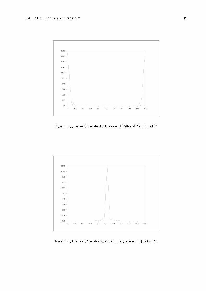
2.4. THE DFT AND THE FFT 49
1 43 86 128 171 213 255 298 340 383 425
0.0
19.3
38.5
57.8
77.0
96.3
115.5
134.8
154.0
173.3
192.5
Figure 2.30: exec('intdec5 10.code') Filtered Version of V
1.0 8.8 16.6 24.4 32.2 40.0 47.8 55.6 63.4 71.2 79.0
-0.00
1.16
2.32
3.48
4.65
5.81
6.97
8.13
9.29
10.45
11.61
Figure 2.31: exec('intdec5 10.code') Sequence x(nMT=L)

50 CHAPTER 2. REPRESENTATION OF SIGNALS
DFT from its de�nition requires order N2 multiplications whereas the FFT requires order N log2Nmultiplications. In this section we discuss several uses of the DFT and some examples of itscalculation using the FFT primitive in Lab.
We begin with the de�nition of the DFT for a �nite length sequence, x(n), of length N ,
X(k) =N�1Xn=0
x(n)e�j2�Nnk : (2.45)
A careful examination of (2.45) reveals that X(k), the DFT of x(n), is periodic with period N (dueto the fact that for �xed n the term exp(�j2�nk=N) is periodic with period N). That X(k) isperiodic also follows from the fact that (2.45) can be interpreted as samples of the z-transform ofx(n) at N equally spaced spaced samples on the unit circle. For reasons of symmetry, the DFT isde�ned to consist of the N distinct points of X(k) for k = 0; 1; : : : ; N � 1.
The N points of the sequence x(n) can be recovered from N points of X(k). This recovery iscalled the inverse DFT and takes the form
x(n) =1
N
N�1Xk=0
X(k)ej2�Nnk: (2.46)
It should be noted that (2.46) yields a periodic sequence in n of period N and that it is the Nvalues of x(n), n = 0; 1; : : : ; N � 1 which yield the desired �nite length sequence.
In order to better understand the DFT, one can think of (2.45) as being represented by a matrixcomputation
266664
X(1)X(2)...
X(N � 1)
377775 =
2666666664
1 1 1 � � � 1
1 e�j2�N e�j
4�N � � � e�j
2(N�1)�N
1 e�j4�N e�j
8�N � � � e�j
4(N�1)�N
......
......
1 e�j2(N�1)�
N e�j4(N�1)�
N � � � e�j(N�1)2�
N
3777777775
266664
x(1)x(2)...
x(N � 1)
377775 : (2.47)
The inverse DFT can be calculated in a similar fashion, where the matrix used is the Hermitiantranspose of that in (2.47) times a factor of 1=N . From (2.47) it can be seen that the DFTrequires order N2 multiplications. The most direct application of the DFT is the calculation ofthe spectrum of �nite length discrete signals. In fact, the DFT is a projection of x(n) onto theorthogonal basis consisting of the N complex exponentials exp(�j2�nk=N) indexed by k. Anotherimportant property of the DFT has to do with the inverse DFT of the product of two transformedsequences. Taking x(n) and h(n) to be two sequences of length N the DFT's of these two sequencesare
X(k) =N�1Xn=0
x(n)e�j2�Nnk (2.48)
and
H(k) =N�1Xn=0
h(n)e�j2�Nnk : (2.49)
Taking the inverse DFT of the product Y (k) = H(k)X(k) yields
y(n) =1
N
N�1Xk=0
H(k)X(k)ej2�Nnk

2.4. THE DFT AND THE FFT 51
=N�1Xm=0
h(m)N�1Xr=0
x(r)1
N
N�1Xk=0
ej2�N(n�m�r)k
=N�1Xm=0
h(m)x(n�m) (2.50)
where the last equality follows from the fact that
1
N
N�1Xk=0
ej2�N(n�m�r)k =
(1; r = n �m
0; otherwise: (2.51)
In (2.50) it should be noted that when the argument of x is outside of the the range [0; N � 1]that the value of x is obtained from evaluating the argument modulo N (which follows from theperiodicity of the x obtained by using the inverse DFT). A very important application of the DFTis for calculating the interaction of discrete signals and discrete linear systems. When a discretesignal is introduced to the input of a linear system, the resulting output is a convolution of theinput signal with the impulse response of the linear system. The convolution operation, which isdiscussed in more detail in the section on convolution, requires order N2 multiplications where thesignal and system impulse response are both of length N . Calculating the convolution by FFTrequires order N log2N multiplications.
It is equally possible to compute a multi-dimensional DFT. For a multi-dimensional sequencex(n1; n2; : : : ; nM) the multi-dimensional DFT is de�ned by
X(k1; k2; : : : ; kM) =N1�1Xn1=1
e�j 2�
N1n1k1
N2�1Xn2=1
e�j 2�
N2n2k2 � � �
NM�1XnM=1
e�j 2�
NMnMkMx(n1; n2; : : : ; nM): (2.52)
The inverse multi-dimensional DFT is analogous to the calculation above with a change of sign forthe complex exponentials and a factor of 1=(N1N2 � � �NM).
The FFT algorithm is a computationally e�cient way of calculating the DFT. The computa-tional savings realized by the FFT are obtained by exploiting certain symmetries and periodicitieswhich exist in the calculation of the DFT. To show how the FFT exploits these properties of theDFT we assume that N = 2 for a positive integer and we calculate the DFT of x(n) as follows
X(k) =N�1Xn=0
x(n)e�j2�Nnk
=X
n=even
x(n)e�j2�Nnk +
Xn=odd
x(n)e�j2�Nnk
=
N2 �1Xr=0
x(2r)e�j 2�
N=2 rk + ej2�Nk
N2 �1Xr=0
x(2r+ 1)e�j 2�
N=2 rk (2.53)
where the �nal equality is obtained by making the change of variables n = 2r. The expression in(2.53) is composed of a sum of two N=2 point DFT's, one for the N=2 point sequence x(0), x(2),: : :, x(N � 2), and the other for the N=2 point sequence x(1), x(3), : : :, x(N � 1). An addition tothe two N=2 point DFT's in (2.53), the calculation also requires N additional multiplications forthe N terms exp(j2�k=N), k = 0; 1; : : : ; N � 1.
The purpose of calculating the DFT as in (2.53) is that a computational savings has beenrealized. As has already been shown the calculation of the N point DFT from (2.45) requires order

52 CHAPTER 2. REPRESENTATION OF SIGNALS
N2 multiplications. Since (2.53) requires the calculation of two N=2 point DFT's plus N additionalmultiplications, the computational load is of order 2(N=2)2 + N = N2=2 + N . For > 1 (i.e.,for N � 4) we have realized a computational savings by using (2.53). Furthermore, the operationin (2.53) can be repeated in that each of the N=2 point DFT's can be split into two N=4 pointDFT's plus N additional multiplications. This yields a computational complexity of 4(N=4)2+2Nmultiplications. Continuing in this way = log2N times, the �nal result is an algorithm withcomputational complexity of N log2N multiplications.
The above discussion of the computational advantages of the FFT is based on the assumptionthat N = 2 . Similar developments of the FFT can be derived based on any prime factorization ofN . The more prime factors N has the greater computational e�ciency can be obtained in using theFFT. In fact, it may be useful in some applications to arti�cially extend the length of a sequence(by adding on zeros) in order that the length of the sequence will be more factorable. The FFTprimitive in Lab automatically accounts for the prime factorization of the sequence length.
2.4.2 Examples Using the fft Primitive
Two examples are presented in this section. The �rst example illustrates how to use the fft
primitive to calculate a one-dimensional DFT. The second example calculates a three-dimensionalDFT.
For the �rst example, data from a cosine function is passed to the fft primitive.
-->//Simple use of fft
-->x=0:63;y=cos(2*%pi*x/16);
-->yf=fft(y,-1);
-->plot(x,real(yf)');
-->xend(),
The cosine data is displayed in Figure 2.32. resulting output from the fft primitive is displayed inFigure 2.33. Figure 2.33 displays the magnitude of the DFT.
Note, however, that since the cosine function is an even symmetric function, the DFT of thecosine is strictly real and, thus, the magnitude and the real part of the DFT are the same. Further-more, since we are calculating a 64-point DFT of a cosine with frequency 2�=16 it is expected thatthe DFT should have peaks at k = 4 and k = 60. This follows from the fact that the value k = 64of the DFT corresponds to a frequency of 2� and, consequently, the value k = 4 must correspondto the frequency 2�=16, which is the frequency of the signal under examination.
The second example calculates the DFT of a three-dimensional signal. The calculation proceedsas follows.
-->y1=matrix(1:6,2,3)
y1 =
! 1. 3. 5. !
! 2. 4. 6. !

2.4. THE DFT AND THE FFT 53
0.00 6.30 12.60 18.90 25.20 31.50 37.80 44.10 50.40 56.70 63.00
-1.0
-0.8
-0.6
-0.4
-0.2
0.0
0.2
0.4
0.6
0.8
1.0
Figure 2.32: exec('fft1.code') Cosine Signal
0.00 6.30 12.60 18.90 25.20 31.50 37.80 44.10 50.40 56.70 63.00
-0.0
3.2
6.4
9.6
12.8
16.0
19.2
22.4
25.6
28.8
32.0
Figure 2.33: exec('fft2.code') DFT of Cosine Signal

54 CHAPTER 2. REPRESENTATION OF SIGNALS
-->y2=matrix(7:12,2,3)
y2 =
! 7. 9. 11. !
! 8. 10. 12. !
-->y=matrix([y1,y2],1,12)
y =
column 1 to 11
! 1. 2. 3. 4. 5. 6. 7. 8. 9. 10. 11. !
column 12
! 12. !
-->yf=mfft(y,-1,[2 3 2])
yf =
column 1 to 7
! 78. - 6. - 12. + 6.9282032i 0 - 12. - 6.9282032i 0 - 36. !
column 8 to 12
! 0 0 0 0 0 !
-->yf1=matrix(yf(1:6),2,3)
yf1 =
! 78. - 12. + 6.9282032i - 12. - 6.9282032i !
! - 6. 0 0 !
-->yf2=matrix(yf(7:12),2,3)
yf2 =
! - 36. 0 0 !
! 0 0 0 !
In the above series of calculations the signal y is three-dimensional and is represented by the twomatrices y1 and y2. The �rst dimension of y are the rows of the matrices, the second dimensionof y are the columns of the matrices, and the third dimension of y are the sequence of matricesrepresented by y1 and y2. The signal y is represented by the vector y which is in vector form. The

2.5. CONVOLUTION 55
x(t) - h(t) -y(t) =Rh(t� u)x(u)du
Figure 2.34: Convolution Performed by Linear System
DFT of y is calculated using the function mfft where flag = �1 and dim = [2 3 2]. Naturally, theDFT of the three-dimensional signal is itself three-dimensional. The result of the DFT calculationis represented by the two matrices yf1 and yf2.
2.5 Convolution
2.5.1 Introduction
Given two continuous time functions x(t) and h(t), a new continuous time function can be obtainedby convolving x(t) with h(t).
y(t) =Z1
�1
h(t� u)x(u)du: (2.54)
An analogous convolution operation can be de�ned for discrete time functions. Letting x(n)and h(n) represent discrete time functions, by the discrete time convolution gives y(n) is :
y(n) =1X
k=�1
h(n � k)x(k): (2.55)
If h(t) represents the impulse response of a linear, time-invariant system and if x(t) is an inputto this system then the output of the system, y(t), can be calculated as the convolution betweenx(t) and h(t) (i.e., as in (2.54). Figure 2.34 illustrates how convolution is related to linear systems.If the system, h(t) is causal (i.e., h(t) = 0 for t < 0) and, in addition, the signal x(t) is applied tothe system at time t = 0, then (2.54) becomes
y(t) =
Z t
0h(t� u)x(u)du: (2.56)
Similarly, for h(n) a time invariant, causal, discrete linear system with input x(n) starting at timen = 0, the output y(n) is the convolution
y(n) =nX
k=0
h(n� k)x(k): (2.57)
An important property of the convolution operation is that the calculation can be e�ected byusing Fourier transforms. This is due to the fact that convolution in the time domain is equivalentto multiplication in the frequency domain. Let X(!), H(!), and Y (!) represent the Fouriertransforms of x(t), h(t), and y(t), respectively, where
Y (!) =Z1
�1
y(t)e�j!tdt: (2.58)
If the relationship in (2.54) is valid, then it also follows that
Y (!) = H(!)X(!): (2.59)
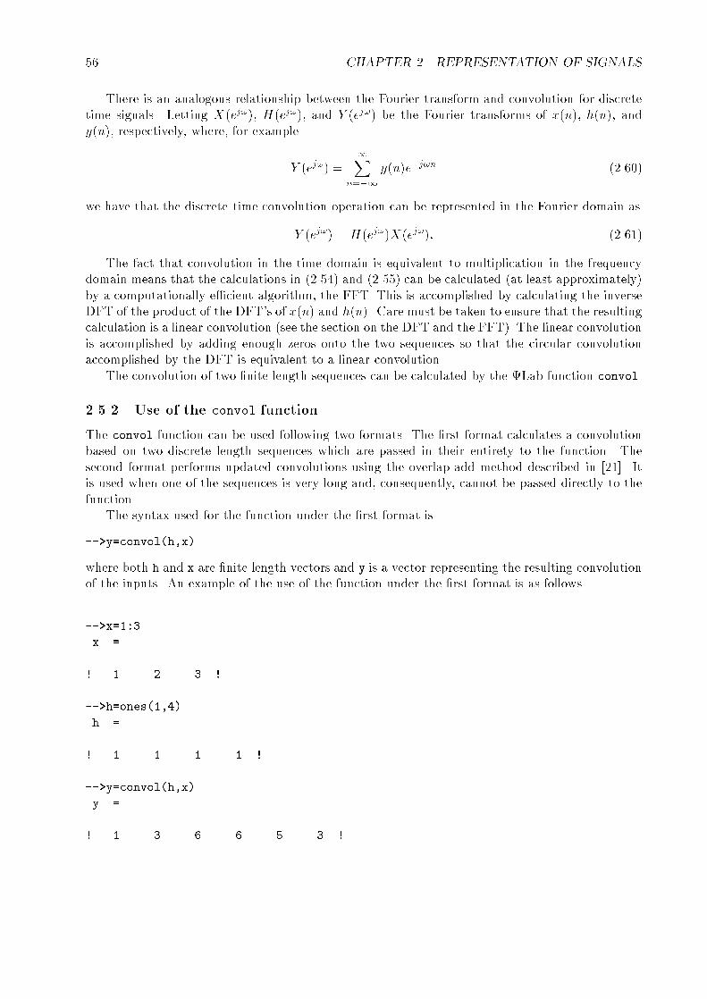
56 CHAPTER 2. REPRESENTATION OF SIGNALS
There is an analogous relationship between the Fourier transform and convolution for discretetime signals. Letting X(ej!), H(ej!), and Y (ej!) be the Fourier transforms of x(n), h(n), andy(n), respectively, where, for example
Y (ej!) =1X
n=�1
y(n)e�j!n (2.60)
we have that the discrete time convolution operation can be represented in the Fourier domain as
Y (ej!) = H(ej!)X(ej!): (2.61)
The fact that convolution in the time domain is equivalent to multiplication in the frequencydomain means that the calculations in (2.54) and (2.55) can be calculated (at least approximately)by a computationally e�cient algorithm, the FFT. This is accomplished by calculating the inverseDFT of the product of the DFT's of x(n) and h(n). Care must be taken to ensure that the resultingcalculation is a linear convolution (see the section on the DFT and the FFT). The linear convolutionis accomplished by adding enough zeros onto the two sequences so that the circular convolutionaccomplished by the DFT is equivalent to a linear convolution.
The convolution of two �nite length sequences can be calculated by the Lab function convol.
2.5.2 Use of the convol function
The convol function can be used following two formats. The �rst format calculates a convolutionbased on two discrete length sequences which are passed in their entirety to the function. Thesecond format performs updated convolutions using the overlap-add method described in [21]. Itis used when one of the sequences is very long and, consequently, cannot be passed directly to thefunction.
The syntax used for the function under the �rst format is
-->y=convol(h,x)
where both h and x are �nite length vectors and y is a vector representing the resulting convolutionof the inputs. An example of the use of the function under the �rst format is as follows.
-->x=1:3
x =
! 1. 2. 3. !
-->h=ones(1,4)
h =
! 1. 1. 1. 1. !
-->y=convol(h,x)
y =
! 1. 3. 6. 6. 5. 3. !

2.6. THE CHIRP Z-TRANSFORM 57
The syntax used for the function under the second format is
-->[y,y1]=convol(h,x,y0)
where y0 and y1 are required to update the calculations of the convolution at each iteration andwhere the use of the second format requires the following function supplied by the user.
//exec('convol1.code')
x1=getx(xlen_1,xstart_1);
[y,y1]=convol(h,x1);
for k=2:nsecs-1,
xk=getx(xlen_k,xstart_k);
[y,y1]=convol(h,xk,y1);
end,
xn=getx(xlen_n,xstart_n);
y=convol(h,xn,y1);
where, nsecs is the number of sections of x to be used in the convolution calculation and, inaddition, the user must supply a function getx which obtains segments of the data x following theformat.
function [xv]=getx(xlen,xstart)
.
.
.
where xlen is the length of data requested and xstart is the length of the data vector to be used.
2.6 The Chirp Z-Transform
2.6.1 Introduction
The discrete Fourier transform (DFT) of a �nite length, discrete time signal, x(n), is de�ned by
X(k) =N�1Xn=0
x(n)e�j(2�nk)=N (2.62)
k = 0; 1; : : : ; N � 1
and the z-transform of x(n) is given by
X(z) =1X
n=�1
x(n)z�n
=N�1Xn=0
x(n)z�n (2.63)
The N�1 points of the DFT of x(n) are related to the z-transform of x(n) in that they are samplesof the z-transform taken at equally spaced intervals on the unit circle in the z-plane.
There are applications [25] where it is desired to calculate samples of the z-transform at locationseither o� the unit circle or at unequally spaced angles on the unit circle. The chirp z-transform

58 CHAPTER 2. REPRESENTATION OF SIGNALS
(CZT) is an e�cient algorithm which can be used for calculating samples of some of these z-transforms. In particular, the CZT can be used to e�ciently calculate the values of the z-transformof a �nite-length, discrete-time sequence if the z-transform points are of the form
zk = AW�k (2.64)
where
A = A0ej�
W = W0e�j� (2.65)
and where A0 and W0 are real valued constants and � and � are angles. The set of points
◊
◊
◊◊
◊◊◊◊◊
◊
◊◊◊◊◊◊◊
◊◊
◊
Figure 2.35: exec('czt1.code') Samples of the z-transform on Spirals
fzkg lie on a spiral where z0 is at distance A0 from the origin and at angle � from the x-axis. Theremaining points are located at equally spaced angles, �, and approach the origin for W0 > 1, moveaway from the origin for W0 < 1, and remain on a circle of radius A0 for W0 = 1. Figure 2.35shows the location of samples of the z-transform for W0 < 1 on the left hand side of the �gure andof W0 < 1 on the right hand side of the �gure. In both parts of the �gure the position of z0 isindicated by the sample connected to the origin by a straight line.
2.6.2 Calculating the CZT
Calculating samples of the z-transform of x(n) at the M points designated in (2.65) requires that
X(zk) =N�1Xn=0
x(n)A�nWnk ; k = 0; 1; : : : ;M � 1 (2.66)
where N is the length of x(n). Using the identity
nk =1
2[n2 + k2 � (k � n)2] (2.67)

2.6. THE CHIRP Z-TRANSFORM 59
x(n) - i- h(n) - i-X(k)6
1=h(k)
6
A�n=h(n)
Figure 2.36: Filter Realization of CZT
in (2.66) yields
X(zk) =N�1Xn=0
x(n)A�nW12n
2W
12k
2W�
12 (k�n)
2
= W12k
2N�1Xn=0
[x(n)A�nW12n
2W�
12 (k�n)
2]: (2.68)
It can be seen that imbedded in (2.68) is a convolution of two sequences g(n) and h(n) where
g(n) = x(n)A�nW12n
2(2.69)
andh(n) = W�
12n2 : (2.70)
Consequently, (2.68) can be represented by the block diagram in Figure 2.36. (The circular junctionsin Figure 2.36 represent multiplication of the two incoming signals).
The convolution in (2.68) can be e�ciently implemented using an FFT. Since the input sequenceis of length N and the output sequence is of length M , it is necessary to use N +M � 1 elementsfrom h(n). These N +M�1 elements are h(�N+1); h(�N+2); : : : ; h(n); : : : ; h(M�2); h(M�1).After taking the product of the N+M �1 point FFT of h(n) and of g(n) (whereM �1 zero pointshave been added to the end of g(n)), the inverse FFT yields a circular convolution of h(n) andg(n). Care must be taken to choose the correct M points corresponding to the linear convolutiondesired. The function czt implements the chirp z-transform.
2.6.3 Examples
The �rst example presented here calculates the CZT of the sequence x(n) = n for n = 0; 1; : : : ; 9where ten points are calculated in the z-plane and the parameter values are W = 1, � = 2�=10,A = 1, and � = 0. This example should yield results identical to those obtained by taking the FFTof the sequence x(n). The sequence of commands is as follows,

60 CHAPTER 2. REPRESENTATION OF SIGNALS
-->[czx]=czt((0:9),10,1,2*%pi/10,1,0);
-->czx'
ans =
! 45. + 4.996D-15i !
! - 5. - 15.388418i !
! - 5. - 6.8819096i !
! - 5. - 3.6327126i !
! - 5. - 1.6245985i !
! - 5. + 6.860D-15i !
! - 5. + 1.6245985i !
! - 5. + 3.6327126i !
! - 5. + 6.8819096i !
! - 5. + 15.388418i !
As can be veri�ed using the function fft, the above result is identical to that obtained by takingthe FFT of the sequence x(n) which is shown below,
-->fft((0:9),-1)'
ans =
! 45. !
! - 5. - 15.388418i !
! - 5. - 6.8819096i !
! - 5. - 3.6327126i !
! - 5. - 1.6245985i !
! - 5. !
! - 5. + 1.6245985i !
! - 5. + 3.6327126i !
! - 5. + 6.8819096i !
! - 5. + 15.388418i !
The second example calculates the DFT of the same sequence, x(n), above, however, just at�ve equally spaced points in [��=4; �=4] on the unit circle in the z-plane. The spacing between thepoints is �=8 for �ve points in [��=4; �=4]. The result is
-->x=0:9;
-->[czx]=czt(x,5,1,%pi/8,1,-%pi/4);
-->czx'
ans =

2.6. THE CHIRP Z-TRANSFORM 61
! 10.363961 + 3.2928932i !
! - 25.451987 - 16.665207i !
! 45. + 4.619D-14i !
! - 25.451987 + 16.665207i !
! 10.363961 - 3.2928932i !
Now taking a sixteen point FFT of the sequence x(n) (accomplished by adding six zeros to theend of the sequence x(n)) it can be seen that the CZT computed above yields exactly the desiredpoints on the unit circle in the z-plane. That is to say that the last three points of czx correspondto the �rst three points of the FFT of x(n) and the �rst two points of czx correspond to the lasttwo points of the FFT.
-->y=0*ones(1:16);
-->y(1:10)=0:9;
-->fft(y,-1)'
ans =
! 45. !
! - 25.451987 + 16.665207i !
! 10.363961 - 3.2928932i !
! - 9.0640653 - 2.3284927i !
! 4. + 5.i !
! - 1.2790805 - 5.6422012i !
! - 2.363961 + 4.7071068i !
! 3.7951327 - 2.6485014i !
! - 5. !
! 3.7951327 + 2.6485014i !
! - 2.363961 - 4.7071068i !
! - 1.2790805 + 5.6422012i !
! 4. - 5.i !
! - 9.0640653 + 2.3284927i !
! 10.363961 + 3.2928932i !
! - 25.451987 - 16.665207i !

62 CHAPTER 2. REPRESENTATION OF SIGNALS

Chapter 3
Design of Finite Impulse Response
Filters
3.1 Windowing Techniques
In theory, the design of FIR �lters is straightforward. One takes the inverse Fourier transform ofthe desired frequency response and obtains the discrete time impulse response of the �lter accordingto (3.1)
h(n) =1
2�
Z �
��H(!)ej!nd! �1 < n <1 (3.1)
The problem, in practice, is that for many �lters of interest the resulting impulse response is in�niteand non-causal. An example of this is the low pass �lter which, given its cut-o� frequency, !c, isde�ned by
H(!j!c) =(
1; j!j � !c0; otherwise
(3.2)
The associated impulse response is obtained by applying (3.1) to (3.2) which yields
h(nj!c) = 1
�nsin(!cn) �1 < n <1 (3.3)
A technique for obtaining a �nite length implementation to (3.3) is to take the N elements of h(n)which are centered around n = 0 and to discard all the remaining elements. This operation can berepresented by multiplying the sequence in (3.3) by an appropriately shifted version of a rectangularwindow of the form
RN(n) =
(1; 0 � n � N � 10; otherwise
(3.4)
The magnitude of the resulting windowed sequence frequency response is depicted in Figure 3.1superimposed on the ideal frequency response (the dotted curve). The �lter illustrated in Figure 3.1has length N = 33 and a cut-o� frequency of !c = :2. As can be seen, the approximation ismarked by a ripple in both the pass and stop bands. This ripple �nds its greatest deviations nearthe discontinuity at !c. The observed ripple is due to the convolution of the ideal frequency responsegiven by (3.2) with the frequency response of the rectangular window. For many applications theripples in the frequency response of Figure 3.1 are unacceptable.
It is possible to decrease the amount of rippling by using di�erent types of windows. Theperformance of a window is governed by its frequency response. Since the frequency response of thewindow is convolved with the desired frequency response the objective is to �nd a window which
63

64 CHAPTER 3. FIR FILTERS
0.00 0.05 0.10 0.15 0.20 0.25 0.30 0.35 0.40 0.45 0.50
0.000
0.108
0.216
0.324
0.433
0.541
0.649
0.757
0.865
0.973
1.081
Figure 3.1: exec('fir1.code') Rectangularly windowed low-pass �lter
has a frequency response which is as impulsive as possible. That is, the frequency response shouldhave a narrow main lobe with most of the energy in this lobe and side lobes which are as smallas possible. The width of the main lobe governs, for example, the width of the transition bandbetween the pass and stop bands of a low pass �lter. The side lobes govern the amount ripple inthe pass and stop bands. The area under the main lobe governs the amount of rejection availablein the stop bands.
The choice of window in the design process is a matter of trading o�, on one hand, the e�ectsof transition band width, ripple, and rejection in the stop band with, on the other hand, the �lterlength and the window type.
3.1.1 Filter Types
The Lab function wfir designs four di�erent types of FIR linear phase �lters: low pass, high pass,band pass, and stop band �lters. The impulse response of the three latter �lters can be obtainedfrom the low pass �lter by simple relations and the impulse response of the low pass �lter is givenin (3.3).
To show the relationship between the four �lter types we �rst examine Figure 3.2 which illus-trates the frequency response of a low pass �lter with cut o� frequency denoted by !l. Thefrequency response of a high pass �lter is illustrated in Figure 3.3 where !h denotes, also, thecut o� frequency. Taking the functional form of the low pass �lter to be H(!j!l) and that of thehigh pass �lter to be G(!j!h), the relationship between these two frequency responses is
G(!j!h) = 1�H(!j!h): (3.5)
Using the result in (3.3), the impulse response of the high pass �lter is given by
g(nj!h) = �(n)� h(nj!h) (3.6)
= �(n)� 1
n�sin(!hn) (3.7)

3.1. WINDOWING TECHNIQUES 65
-3.14 -2.51 -1.88 -1.26 -0.63 0.00 0.63 1.26 1.88 2.51 3.14
-0.125
0.000
0.125
0.250
0.375
0.500
0.625
0.750
0.875
1.000
1.125
Figure 3.2: exec('fir2 5.code') Frequency response of a low pass �lter
-3.14 -2.51 -1.88 -1.26 -0.63 0.00 0.63 1.26 1.88 2.51 3.14
-0.125
0.000
0.125
0.250
0.375
0.500
0.625
0.750
0.875
1.000
1.125
Figure 3.3: exec('fir2 5.code') Frequency response of a high pass �lter

66 CHAPTER 3. FIR FILTERS
where �(n) = 1 when n = 0 and is zero otherwise.For a band pass �lter, as illustrated in Figure 3.4, the functional form of the frequency
-3.14 -2.51 -1.88 -1.26 -0.63 0.00 0.63 1.26 1.88 2.51 3.14
-0.125
0.000
0.125
0.250
0.375
0.500
0.625
0.750
0.875
1.000
1.125
Figure 3.4: exec('fir2 5.code') Frequency response of a band pass �lter
response, F (!j!l; !h) can be obtained by shifting the low pass �lter two times as follows
F (!j!l; !h) = H(! � !1j!2) +H(! + !1j!2) (3.8)
!1 =1
2(!l + !h) (3.9)
!2 =1
2(!l � !h): (3.10)
Thus, the impulse response of the band pass �lter is
f(nj!l; !h) = ej!1nh(nj!2) + e�j!1nh(nj!2) (3.11)
=2
n�cos(!1n) sin(!2n): (3.12)
Finally, the stop band �lter illustrated in Figure 3.5 can be obtained from the band pass�lter by the relation
D(!j!l; !h) = 1� F (!j!l; !h) (3.13)
where D(!j!l; !h) is the frequency response of the stop band �lter. The impulse response of this�lter is
d(nj!l; !h) = �(n)� f(nj!l; !h) (3.14)
= �(n)� 2
n�cos(!1n) sin(!2n): (3.15)
3.1.2 Choice of Windows
Four types of windows are discussed here. They are the triangular, generalized Hamming, Kaiser,and Chebyshev windows. As was noted in the introduction it is the frequency response of a window

3.1. WINDOWING TECHNIQUES 67