A Pragmatic Introduction to Signal Processing

with applications in Chemical Analysis

An illustrated essay with software available for free download

Last updated April 30, 2014. Latest version available online at:

PDF format: http://terpconnect.umd.edu/~toh/spectrum/IntroToSignalProcessing.pdf

Web address: http://terpconnect.umd.edu/~toh/spectrum/TOC.html

Tom O'HaverProfessor Emeritus

Department of Chemistry and BiochemistryUniversity of Maryland at College Park

E-mail: toh@umd.edu

© T. C. O'Haver, 1997, 2014

Table of ContentsIntroduction 2Signal arithmetic 3Signals and noise 6Smoothing 11Differentiation 17Resolution enhancement 26Harmonic analysis 28Convolution 31Deconvolution 32Fourier filter 34Integration and peak area measurement 35Linear least-squares curve fitting 37Multicomponent spectroscopy 49Non-linear iterative curve fitting 54Software details: SPECTRUM for Macintosh OS8 70Software details: Matlab and Octave for PC/Mac/Linux 73 Peak finding and measurement: findpeaks and iPeak 74 Interactive smooth, derivative, sharpen, etc: iSignal 85 Iterative peak fitting: peakfit and ipf 90Hyperlinear absorption spectroscopy 103Appendix: More on Smoothing 110Case Studies 112References 117Alphabetical Index 119

1

IntroductionThe interfacing of analytical measurement instrumentation to small computers for the purpose of on-line data acquisition has now become standard practice in the modern laboratory. Using widely-available, low-cost microcomputers and off-the-shelf add-in components, it is now easier than ever to acquire data quickly in digital form.

Computerized digital data acquisition has some obvious advantages over old methods, such as archival storage and retrieval of data and post-run re-plotting with adjustable scale expansion. Computer memory is cheaper that paper and digital data can be more easily duplicated without error. Plus, there is the possibility of performing post-run data analysis and signal processing. There are a large number of computer-based numerical methods that can be used to transform signals into more useful forms, detect and measure peaks, reduce noise, improve the resolution of overlapping peaks, compensate for instrumental artifacts, test hypotheses, optimize measurement strategies, diagnose measurement difficulties, and decompose complex signals into their component parts. These techniques can often make difficult measurements easier by extracting more information from the available data. Many of these techniques are based on laborious mathematical procedures that were not practical before the advent of computerized instrumentation. As computers have become faster, cheaper, and more widely available, many of these techniques are now routine. It is important for students to appreciate the capabilities as well as the limitations of these signal processing techniques.

In the chemistry curriculum, signal processing may be covered as part of a course on instrumental analysis (1, 2), electronics for chemists (3), laboratory interfacing (4), or basic chemometrics (5). The purpose of this paper is to give a practical introduction to some of the most widely used signal processing techniques and to give illustrations of their applications in analytical chemistry. This essay covers only elementary topics and is limited to mathematics only through elementary calculus and matrix math. (For the math-phobic, this paper contains more than twice as many figures as equations). At the present time, this work does not yet cover wavelet transforms, pattern recognition, or factor analysis. For more advanced topics and for a more rigorous treatment of the underlying mathematics, refer to the extensive literature on chemometrics (references, page 117).

This tutorial makes extensive use of Matlab, a high-performance commercial numerical computing environment and programming language that is widely used by scientists, researchers, and engineers, and Octave, a free Matlab alternative that runs almost all of the Matlab examples in this document without change (see page 73). There are Windows, Mac, and Unix versions of Octave; the Windows version can be downloaded from Octave Forge. (Installation of Octave is somewhat more laborious than installing a commercial package like Matlab; be sure to install all the Octave Forge “packages” that add essential functions. Octave is also slower that Matlab computationally - about half as fast for computations and about 5 times slower for 2D graphics).

Some of the examples were developed in spreadsheets such as Excel and OpenOffice Calc and an old freeware Macintosh signal-processing program called SPECTRUM (see page 70).

Paragraphs in gray at the end of each section in this essay describe the related capabilities of each of these programs, including my own signal-processing modules written for Matlab and Octave that you can download for your own use. For descriptions and download links to the latest versions of my downloadable spreadsheets and Matlab/Octave scripts and functions, go to http://tinyurl.com/cey8rwh. Pages 70 to 111 of this document contain instructions for the operation of these software modules and many examples of their applications. Descriptions of my downloadable interactive signal processing tools (for Matlab only) are described on http://terpconnect.umd.edu/~toh/spectrum/SignalProcessingTools.html

This document and its associated software are undated regularly. If you are reading this off-line, there is probably a newer version already. For the latest on-line version, in printed and on-line formats, go to http://terpconnect.umd.edu/~toh/spectrum/.

2

Signal arithmeticThe most basic signal processing functions are those that involve simple signal arithmetic: point-by-point addition, subtraction, multiplication, or division of two signals or of one signal and a constant. Despite their mathematical simplicity, these functions can be very useful. For example, in the left part of the figure below, the top curve is the absorption spectrum of an extract of a sample of oil shale, a kind of rock that is a source of petroleum.

A simple point-by-point subtraction of two signals allows the background (bottom curve on the left) to be subtracted from a complex sample (top curve on the left), resulting in a clearer picture of what is

really in the sample (right).

This spectrum exhibits two absorption bands, at about 515 nm and 550 nm, that are due to a class of molecular fossils of chlorophyll called porphyrins. (Porphyrins are used as geomarkers in oil exploration). These bands are superimposed on a background absorption caused by the extracting solvents and by non-porphyrin compounds extracted from the shale. The bottom curve is the spectrum of an extract of a shale that does not contain porphyrins, showing only the background absorption.

To obtain the spectrum of the shale extract without the background, the background (bottom curve) is simply subtracted from the sample spectrum (top curve). The difference is shown in the right in Window 2 (note the change in Y-axis scale). In this case the removal of the background is not perfect, because the background spectrum is measured on a separate shale sample. However, it works well enough that the two bands are now seen more clearly and it is easier to measure precisely their absorbances and wavelengths.

In this example and the one below, the assumption is being made that the two signals in Window 1 have the same x-axis values, that is, that both spectra are digitized at the same set of wavelengths. This operation would not be valid if the two spectra were digitized over different wavelength ranges or with different intervals between adjacent points. The x-axis values much match up point for point. In practice, this is very often the case with data sets acquired within one experiment on one instrument, but the experimenter must take care if the instruments settings are changed or if data from two experiments or two instrument are combined. (Note: It is possible to use the mathematical technique of interpolation to change the number of points or the x-axis intervals of signals; the results are only approximate but often close enough in practice. The Matlab program iSignal, page 85, includes a convenient interpolation function).

Sometimes you might like to know whether two signals have the same shape, for example in comparing the spectrum of an unknown to a stored reference spectrum. Most likely the concentrations of the unknown and reference, and thus the amplitudes of the spectra, will be different. Therefore a direct overlay or subtraction of the two spectra will not be useful. One

3

possibility is to compute the point-by-point ratio of the two signals; if they have the same shape, the ratio will be a constant. For example, examine this figure:

Do the two spectra on the left have the same shape? They certainly do not look the same, but that may simply be due to that fact that one is much weaker that the other. The ratio of the two spectra, shown in

the right part (Window 2), is relatively constant from 300 to 440 nm, with a value of 10 +/- 0.2. This means that the shape of these two signals is very nearly identical over this wavelength range.

The left part (Window 1) shows two superimposed spectra, one of which is much weaker than the other. But do they have the same shape? The ratio of the two spectra, shown in the right part (Window 2), is relatively constant from 300 to 440 nm, with a value of 10 +/- 0.2. This means that the shape of these two signals is the same, within about +/-2 %, over this wavelength range, and that top curve is about 10 times more intense than the bottom one. Above 440 nm the ratio is not even approximately constant; this is caused by random noise, which is the topic of the next section (page 6).

Simple signal arithmetic operations such as these are easily done in any spreadsheet (e.g. Excel or the freely downloadable OpenOffice Calc), any general-purpose programming language, in a dedicated signal-processing program such as SPECTRUM (Page 70), or (most easily) in a vector-matrix programming language such as Matlab or Octave (Page 73).

Popular spreadsheet programs Excel and Open Office Calc have built-in functions for all common math operations, named variables, x,y plotting, text formatting, basic matrix math, etc. Cells can contain numerical values, text, mathematical expressions (formulas), or references to other cells. A vector of values such as a spectrum can be represented as a row or column of cells; a rectangular array of values such as a set of spectra can be represented as a rectangular block of cells. User-created names can be assigned to individual cells or to ranges of cells, then referred to in formulas by name, which makes the formulas easier to understand. Formulas can be easily copied across a range of cells, with the cell references changing or not as desired. Plots of various types can be created by menu selection. See http://www.youtube.com/watch?v=nTlkkbQWpVk for a nice video demonstration.

The latest versions of both Excel (Excel 2013) and OpenOffice Calc (4.0) can open and save spreadsheet file formats of the other (.xls and .ods, respectively). Simple spreadsheets in either format are compatible with the other program. However, there are small differences in the way that certain functions are interpreted, and for that reason I supply most of my spreadsheets in both .xls (for Excel) and in .ods (for Calc) formats. Basically, Calc 4.0 can do most everything Excel can do, but Calc is free to download and is more Windows-standard in terms of look-and-feel. (Not every science worker who needs a spreadsheet can afford to buy, or has access to a site license for, expensive Microsoft products).

In Matlab and in Octave, math operations on signals are especially powerful because the variables can be either scalar (single values), vector (like a row or a column in a spreadsheet), representing one entire signal, spectrum or chromatogram, or matrix (like a rectangular block of cells in a spreadsheet), representing a set of signals. For example, you could define two vectors a=[1 2 5 2 1] and b=[4 3 2 1 0]. Then to subtract B from A you would just type a-b, which gives the result [-3 -1 3 1

4

1]. To multiply A times B point by point, you would type a.*b, which gives the result [4 6 10 2 0]. If you have an entire spectrum in the variable a, you can plot it just by typing plot(a). And if you also had a vector w of x-axis values (such as wavelengths), you can plot a vs w by typing plot(w,a).

The subtraction of two spectra a and b, as in the figure on page 3, can be performed simply by writing a-b. To plot the difference, you would write plot(w,a-b). Likewise, to plot the ratio of two spectra, as in the figure on page 4, you would write plot(w,a./b). Typing b\a in Matlab will compute the "matrix right divide", in effect the weighted average ratio of the amplitudes of the two vectors - a type of least-squares best-fit solution (page 37) - which in the example in the figure on page 4 will be a single scalar number very close to 10.

The point here is that Matlab and Octave don't require you to deal with vectors and matrices as collections of numbers; it knows when you are dealing with matrices and adjusts your calculations accordingly. See http://www.mathworks.com/help/matlab/matlab_prog/array-vs-matrix-operations.html.

Both Matlab and Octave can be used to automate complex sequences of operations by saving them as scripts and functions (text files saved with a “.m” file name extension). Matlab and Octave are also considerably faster in computations and in graphing than spreadsheets. You can easily import your own data into Matlab or Octave by using the load command. Data can be imported from text files and from spreadsheets. Matlab has a convenient Import Wizard (click File > Import Data).

Spreadsheet or Matlab/Octave? For signal processing, Matlab/Octave is faster and more powerful than spreadsheets, but spreadsheets have their advantages: they are easier for novices and they offer very flexible presentation and user interface design. Spreadsheets are concrete and more low-level, showing every single value explicitly in a cell. In contrast, Matlab/Octave is more high level and abstract, because a single variable or function can do so much. Also, user-defined functions can call other built-in or user-defined functions, which in turn can call other functions, and so on, allowing very complex high-level functions to be built up in layers.

The bottom line is that spreadsheets are easier at first, but sooner or later the Matlab/Octave approach is more productive for most applications. This point is demonstrated by comparing both approaches to multilinear regression in multicomponent spectroscopy (page 51), and especially by the dramatic difference between the spreadsheet and Matlab/Octave approaches to finding and measuring peaks in signals (page 83), i.e. a 250Kbyte spreadsheet vs a 7Kbyte Matlab/Octave script that actually does more.

Both spreadsheets and Matlab/Octave programs have a huge advantage over commercial end-user programs and compiled freeware programs such as SPECTRUM (page 70); they can be inspected and modified by the user to customize the routines for specific needs. Simple changes are easy to make with only modest knowledge of programming. For example, you could easily change the titles or colors or line style of graphs - in Matlab or Octave programs, search for "title(" or "plot(", respectively. My code contains comments that indicate places where specific changes can easily be made: just search for the word "change".

5

Signals and noiseExperimental measurements are never perfect, even with sophisticated modern instruments. Two main types or measurement errors are recognized: (a) systematic error, in which every measurement is consistently less than or greater than the correct value by a certain amount or relative percentage, and (b) random error, in which there are unpredictable variations in the measured signal from moment to moment or from measurement to measurement. This latter type of error is often called noise, by analogy to acoustic noise. Sources of noise in measurements might include such things as building vibrations, air currents, electric power fluctuations, stray radiation from nearby electrical apparatus, static electricity, interference from radio and TV transmissions, electrical storms, turbulence in the flow of gases or liquids, random thermal motion of electrons or molecules, background radiation from naturally occurring radioactive elements in the environment, “cosmic rays” from outer space (seriously), and even the basic quantum nature of matter and energy itself.

One of the fundamental problems in signal measurement is distinguishing the noise from the signal. It's not always easy. The signal is the “important” part of the data that you want to measure - it might be the average of the signal over a certain time period or the height of a peak or the area under a peak that occurs in the data. For example, in the absorption spectrum in the right-hand half of the figure on page 3 in the previous section, the “important” parts of the data are probably the absorption peaks located at 520 and 550 nm. The height of either of those peaks might be considered the signal, depending on the application. In this example, the height of the largest peak is about 0.08 absorbance units. The noise would be the standard deviation of that peak height from spectrum to spectrum (if you had access to repeat measurements of the same spectrum). But what if you had only one recording of that spectrum? In that case, you'd be forced to estimate the noise in that single recording, based on the visible short-term fluctuations in the signal (the little random wiggles superimposed on the smooth signal), which we assume are noise, based on previous observations that no samples of that type ever exhibit reproducible short-term “fine structure” in their signals. In this case, those fluctuations amount to about 0.005 units peak-to-peak or a standard deviation of 0.001. For random fluctuations, the rule of thumb is that the peak-to-peak variation between the highest and the lowest readings is approximately 5 times the standard deviation, as demonstrated by this line of Matlab code: rn=randn(1,100);(max(rn)-min(rn))/std(rn). As another example, the data on the right half of the figure on the next page has a peak in the center with a height of about 1.0. The peak-to-peak noise on the baseline is also about 1.0, so the standard deviation of the noise is about 1/5th of that, or 0.2.

The quality of a signal is often expressed quantitatively as the signal-to-noise ratio (SNR), which is the ratio of the true signal amplitude (e.g. the average amplitude or the peak height) to the standard deviation of the noise. Thus the signal-to-noise ratio of the spectrum on page 3 is about 0.08/0.001 = 80, and the signal on page 7 has a signal-to-noise ratio of 1.0/0.2 = 5. So we would say that the signal-to-noise ratio of the signal on page 3 is better than that on page 7. Signal-to-noise ratio is inversely proportional to the relative standard deviation of the signal amplitude. Measuring the signal-to-noise ratio is much easier if the noise can be measured separately, in the absence of signal. The relationship between signal-to-noise ratio and the relative standard deviation of the signal amplitude depends on how the signal amplitude is measured, specifically how may data points can be averaged or otherwise used; often (but not always), the relative standard deviation varies with the square root of the number of noisy data points averaged.Depending on the type of experiment, it may be possible to acquire readings of the noise alone,

6

for example on a segment of the baseline before or after the occurrence of the signal. However, if the magnitude of the noise depends on the level of the signal, then the experimenter must try to produce a constant signal level to allow measurement of the noise on the signal. In some cases, where it is possible to model the shape of the signal exactly by means of a mathematical function, the noise may be estimated by subtracting the model signal from the experimental signal, for example by least-squares curve fitting (see page 37). If practical, it's always better to determine the standard deviation of repeated measurements of the quantity that you want to measure, rather than trying to estimate the noise from a single recording of the data.

Window 1 (left) is a single measurement of a very noisy signal. There is actually a broad peak at the center of this signal, but it is not possible to measure its position, width, and height accurately because the signal-to-noise ratio is very poor (less than 1). Window 2 (right) is the average of 9 repeated measurements of this signal, clearly showing the reduction in the amplitude of the noise. The expected improvement in signal-to-noise ratio is 3 (the square root of 9). In some cases it is possible to average hundreds of measurements, resulting in even more substantial improvement.

One key thing that really distinguishes signal from noise is that random noise is not the same from one measurement of the signal to the next, whereas the genuine signal is at least partially reproducible. So if the signal can be measured more than once, use can be made of this fact by measuring the signal over and over again, as fast as is practical, and adding up all the measurements point-by-point, then dividing by the number of signal averaged. This is called ensemble averaging, and it is one of the most powerful methods for improving signals, when it can be applied. For this to work properly, the noise must be random and the signal must occur at the same time in each repeat. An example is shown in the figure above. The signal-to-noise ratio improves with the square root of the number of independent signals added.Sometimes the signal and the noise can be partly distinguished on the basis of frequency components (page 28), that is, how rapidly it changes with time: for example, the signal may contain mostly low-frequency components and most of the noise may be located at higher frequencies. This is the basis of filtering and smoothing (page 11). In the figures above, the peaks contain mostly low-frequency components, whereas the noise is distributed over a much wider frequency range. The frequency characteristic of noise is described by its frequency spectrum. White noise has equal power at all frequencies; it derives its name from white light, which has equal brightness at all wavelengths in the visible region. The noise in the example above, and in the upper left quadrant of the figure on page 8, is white. In the acoustical domain, white noise sounds like a “hiss”. This is a commonly encountered type of noise in measurement science; for example photon noise and Johnson noise are nearly white. Another common type of noise has a low-frequency-weighted character; it has more power at low frequencies that at high frequencies. This is often called “pink noise”. In the acoustical domain, pink noise sounds more like a “roar”. (A sub-species of that type of noise is “1/f noise”, where the noise power in inversely proportional to frequency, shown in the upper right quadrant of the figure on the left, below). Conversely, noise that has more power at high frequencies

7

would be called “blue” noise; it's less common in experimental work and fortunately it's easily reduced by smoothing (page 11).

Pink noise is more troublesome than white or blue noise, because a given standard deviation of pink noise has a greater effect on the accuracy of most measurements than the same standard deviation of white noise (as demonstrated by the Matlab/Octave function noise test.m mentioned on page 10). Moreover, the application of smoothing (page 11) and low-pass filter i ng to reduce noise is more effective for white noise than for pink noise. When pink noise is present, it is sometimes beneficial to apply modulation techniques, such as o ptical chopping or wavelength modulation, to convert a direct-current (DC) signal into an alternating current (AC) signal, thereby increasing the frequency of the signal to a frequency region where the noise is lower. In such cases it is common to use a lock-in amplifier, or the digital equivalent thereof, to measure the amplitude of the signal. (You can download a Matlab/Octave function that demonstrates the appearance of white, pink, proportional, and square-root noise, and their effect on signal measurement, from h ttp://terpconnect.umd.edu/~toh/spectrum/ noise test.m).

Noise can also be characterized by the way it varies with the signal amplitude. It may be a constant “background” noise that is independent of the signal amplitude, or it may vary with the signal, perhaps increasing directly or with the square root of the signal amplitude. For example, in optical spectroscopy, three fundamental types of noise are recognized, based on their origin and on how they vary with light intensity: photon noise, detector noise, and flicker (fluctuation) noise. Photon noise (often the limiting noise in instruments that use photomultiplier detectors) is white and is proportional to the square root of light intensity (illustrated in the lower right quadrant of the figure

above), and therefore the SNR is proportional to the square root of light intensity and directly proportional to the monochromator slit width. Detector noise (often the limiting noise in instruments that use solid-state photodiode or thermal detectors) is independent of the light intensity and therefore the detector SNR is directly proportional to the light intensity and to the square of the monochromator slit width. Flicker noise, caused by light source instability, vibration, sample cell positioning errors, sample turbulence, light scattering by suspended particles, dust, bubbles, etc., is directly proportional to the light intensity (illustrated in the lower left quadrant of the figure above), so the flicker signal-to-noise ratio is not decreased by increasing the slit width. Flicker noise is usually pink rather than white. In practice, the total noise observed is likely to have some contribution of all three types of amplitude dependence, as well as a mixture of white and pink noises.

The key to reducing noise in an experimental system is first to understand the possible sources of noise, break down the system into its parts and measure the noise generated by each part separately, then seek to reduce or compensate for as much of each noise source as possible. For example, in optical spectroscopy, source flicker noise can be reduced by feedback stabilization, choosing an alternative source, using and internal standard, or using specialized instrument designs such as double-beam, dual wavelength, derivative, and wavelength modulation. The effect of photon noise and detector noise can be reduced by increasing the light intensity at the detector, and electronics noise can be reduced by cooling or upgrading the detector and/or electronics.

8

Another property that distinguishes noise is its amplitude probability distribution, the function that describes the probability of a random variable falling within a certain range of values. In physical measurements, the most common distribution is the “Gaussian curve” (also called a “bell” or “haystack” curve) and is described by y = e^(-(x-m)^2/(2 s^2))/(sqrt(2 p) s), where m is the mean (average) value and s is the standard deviation. In this type of distribution, the most common noise errors are small (that is, close to the mean) and the errors become less common the greater their deviation. This is such a commonly-encountered type of distribution that it is called a “normal” distribution.

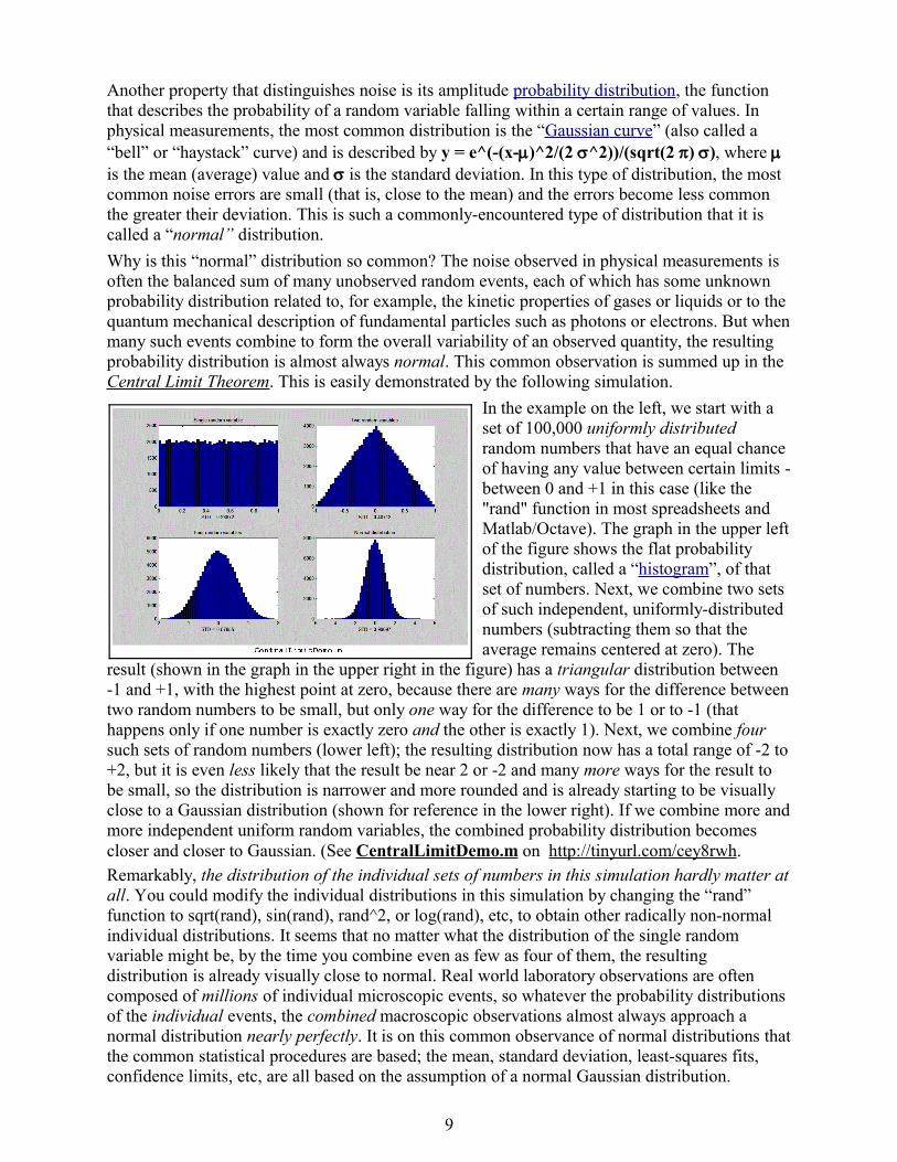
Why is this “normal” distribution so common? The noise observed in physical measurements is often the balanced sum of many unobserved random events, each of which has some unknown probability distribution related to, for example, the kinetic properties of gases or liquids or to the quantum mechanical description of fundamental particles such as photons or electrons. But when many such events combine to form the overall variability of an observed quantity, the resulting probability distribution is almost always normal. This common observation is summed up in the Central Limit Theorem. This is easily demonstrated by the following simulation.

In the example on the left, we start with a set of 100,000 uniformly distributed random numbers that have an equal chance of having any value between certain limits - between 0 and +1 in this case (like the "rand" function in most spreadsheets and Matlab/Octave). The graph in the upper left of the figure shows the flat probability distribution, called a “histogram”, of that set of numbers. Next, we combine two sets of such independent, uniformly-distributed numbers (subtracting them so that the average remains centered at zero). The

result (shown in the graph in the upper right in the figure) has a triangular distribution between -1 and +1, with the highest point at zero, because there are many ways for the difference between two random numbers to be small, but only one way for the difference to be 1 or to -1 (that happens only if one number is exactly zero and the other is exactly 1). Next, we combine four such sets of random numbers (lower left); the resulting distribution now has a total range of -2 to +2, but it is even less likely that the result be near 2 or -2 and many more ways for the result to be small, so the distribution is narrower and more rounded and is already starting to be visually close to a Gaussian distribution (shown for reference in the lower right). If we combine more and more independent uniform random variables, the combined probability distribution becomes closer and closer to Gaussian. (See CentralLimitDemo.m on http://tinyurl.com/cey8rwh.Remarkably, the distribution of the individual sets of numbers in this simulation hardly matter at all. You could modify the individual distributions in this simulation by changing the “rand” function to sqrt(rand), sin(rand), rand^2, or log(rand), etc, to obtain other radically non-normal individual distributions. It seems that no matter what the distribution of the single random variable might be, by the time you combine even as few as four of them, the resulting distribution is already visually close to normal. Real world laboratory observations are often composed of millions of individual microscopic events, so whatever the probability distributions of the individual events, the combined macroscopic observations almost always approach a normal distribution nearly perfectly. It is on this common observance of normal distributions that the common statistical procedures are based; the mean, standard deviation, least-squares fits, confidence limits, etc, are all based on the assumption of a normal Gaussian distribution.

9

It important to understand that the three characteristics of noise just discussed in the paragraphs above - the frequency distribution, the signal dependence, and the amplitude distribution - are mutually independent; a noise may in principle have any combination of those properties.

SPECTRUM (page 70) includes several functions for measuring signals and noise, plus a signal-generator that can be used to generate artificial signals with Gaussian and Lorentzian bands, sine waves, and normally-distributed random noise. Popular spreadsheets, such as Excel or Open Office Calc, have built-in functions that can be used for measuring and plotting signals and noise, such as AVERAGE, MAX, MIN, STDEV (or STD), and RAND. Some spreadsheets have only a uniformly-distributed random number function (rand) and not a normally-distributed random number function (randn), but it's much more realistic to simulate errors that are normally distributed. In that case it's convenient to make use of the Central Limit Theorem to create normally distributed random numbers by combining several uniformly-distributed RAND functions. For example, the expression 1.73*(RAND()-RAND()+RAND()-RAND()) creates nearly normal random numbers with a mean of zero, a standard deviation very close to 1, and a maximum range of ±4. (The alternating + and – signs simply insures that the result averages to zero, and the factor of 1.73 makes the average standard deviation equal to 1.00, as is the case for the normally-distributed RANDN function). The spreadsheets RandomNumbers.xls/.ods and the Matlab/Octave script RANDtoRANDN.m demonstrate how this works. Download from http://tinyurl.com/cey8rwh.Matlab and Octave have built-in functions that are used for measuring and plotting signals and noise, such as plot, mean, max, min, std, hist, histfit, rand, and randn. Just type “help” and the function name at the command prompt, e.g. “help mean”. Most of these Matlab and Octave functions apply to vectors and matrices as well as scalar variables. You can subtract a scalar number from a vector (for example, v = v-min(v) sets the lowest value of vector v to zero). If you have a set of signals in the rows of a matrix S, where each column represents the value of each signal at the same value of the independent variable (for example, time), you can compute the ensemble average of all the columns of S just by typing “mean(S)”.You can also create user-defined functions in Matlab or Octave to automate commonly-used algorithms. For an explanation and a simple worked example, type “help function” at the command prompt. I have created some Matlab/Octave functions related to signal processing: plotfit.m, a simple function for plotting and fitting x,y data in matrices or in separate vectors; a set of functions for peak shapes commonly encountered in analytical chemistry (Gaussian, Lorentzian, etc.) and functions for different types of random noise (white noise, pink noise, proportional noise, and square root noise). There is also a function that applies exponential broadening (ExpBroaden.m) to a signal; a function that computes the i nterquartile range (Iqrange.m); a function that removes “not-a-number” entries from vectors (rmnan.m); and a function that returns the index and the value of the element of vector x that is closest to a particular value (val2ind.m). These functions can be downloaded from http://tinyurl.com/cey8rwh. Once you have downloaded those functions and placed them in the Matlab / Octave path, you can use them just like any other built-in function. For example, you can get help for any function by typing “help <name>”. You can plot a simulated noisy peak Gaussian such as that on page 8: x=[1:256];y=gaussian(x,128,64)+0.2*whitenoise(x);plotfit(x,y)noise test.m is a self-contained Matlab/Octave function that demonstrates different noise types and their effects. It creates a set of Gaussian peaks with different types of added noise: constant white noise, constant pink (1/f) noise, proportional white noise, and square-root white noise. It then fits a Gaussian to each noisy data set and computes the average and the standard deviation of repeated measurements of best-fit peak height, position, width, and area for each noise type.iSignal (page 85) can plot signals with pan and zoom controls, measure signal and noise amplitudes in selected regions of the signal, compute the signal-to-noise ratio of peaks, perform variable smoothing, differentiation, interpolation, peak sharpening, and measurement of the positions, heights, widths, and areas or noisy peaks. It's operated by simple keypresses.For a complete list of my downloadable Matlab and Octave functions, demonstration scripts, and spreadsheets, see http://tinyurl.com/cey8rwh

10

SmoothingIn many experiments in physical science, the true signal amplitudes (y-axis values) change rather smoothly as a function of the x-axis values, whereas many kinds of noise are seen as rapid, random changes in amplitude from point to point within the signal. In the latter situation it is common practice to attempt to reduce the noise by a process called smoothing. In smoothing, the data points of a signal are modified so that individual points that are higher than the immediately adjacent points (presumably because of noise) are reduced, and points that are lower than the adjacent points are increased. This naturally leads to a smoother signal. As long as the true underlying signal is actually smooth, then the true signal will not be much distorted by smoothing, but the noise will be reduced. Smoothing algorithms. Most smoothing algorithms are based on the "shift and multiply" technique, in which a group of adjacent points in the original data are multiplied point-by-point by a set of numbers (coefficients) that defines the smooth shape, the products are added up to become one point of smoothed data, then the set of coefficients is shifted one point down the original data and the process is repeated. The simplest smoothing algorithm is the rectangular or unweighted sliding-average smooth; it simply replaces each point in the signal with the average of m adjacent points, where m is a positive integer called the smooth width. For example, for a 3-point smooth (m=3):

The triangular smooth is like the rectangular smooth, above, except that it implements a weighted smoothing function. For a 5-point smooth (m=5):

for j = 3 to n-2, and similarly for other smooth widths.

It is often useful to apply a smoothing operation more than once, that is, to smooth an already smoothed signal, in order to build longer and more complicated smooths. For example, the 5-point triangular smooth above is equivalent to two passes of a 3-point rectangular smooth. Three passes of a 3-point rectangular smooth result in a 7-point "pseudo-Gaussian" or haystack smooth, for which the coefficients are in the ratio 1 3 6 7 6 3 1. The general rule is that p passes of a m-width smooth results in a combined smooth width of p*m-p+1. For example, 3 passes of a 17-point smooth results in a 49-point smooth. These multipass smooths are more effective at reducing high-frequency noise in the signal than a single rectangular smooth of the same width.In all of these smooths, the width of the smooth m is usually chosen to be an odd integer, so that the smooth coefficients are symmetrically balanced around the central point, which is important point because it preserves the x-axis position of peaks and other features in the signal. (This is especially critical for some analytical and spectroscopic applications because the peak positions are important measurement objectives).

Note that we are assuming here that the x-axis intervals of the signal is uniform, that is, that the difference between the x-axis values of adjacent points is the same throughout the signal. This is also assumed in many of the other signal-processing techniques described in this essay, and it is a very common (but not necessary) characteristic of signals that are acquired by automated and

11

computerized equipment. The Savitzky-Golay smooth is based on the least-squares fitting of polynomials to segments of the data. Compared to the sliding-average smooths, the Savitzky-Golay smooth is less effective at reducing noise, but more effective at retaining the shape of the original signal. The algorithm is more complex and the computational times are greater than the smooth types discussed above, but with modern computers the difference is usually not significant (see page 110). It is capable of differentiation as well as smoothing. Code in various languages is widely available online. Noise reduction. Smoothing can reduce the apparent noise in a signal. If the noise is “white” (that is, evenly distributed over all frequencies) and its standard deviation is s, then the standard deviation of the noise remaining in the signal after one pass of a triangular smooth will be approximately s*0.8/sqrt(m), where m is the smooth width. Smoothing operations can be applied more than once: that is, a previously-smoothed signal can be smoothed again. In some cases this can be useful if there is a great deal of high-frequency noise in the signal. However, the noise reduction for white noise is less less in each successive smooth; three passes of a rectangular smooth reduces white noise by a factor of s*0.7/sqrt(m), only a slight improvement over two passes. Edge effects and the lost points problem. Note in the equations above that the 3-point rectangular smooth is defined only for j = 2 to n-1. There is not enough data in the signal to define a complete 3-point smooth for the first point in the signal (j = 1) or for the last point (j = n) , because there are no data points before the first point or after the last point. Similarly, a 5-point smooth is defined only for j = 3 to n-2, and therefore a smooth can not be calculated for the first two points or for the last two points. In general, for an m-width smooth, there will be (m-1)/2 points at the beginning of the signal and (m-1)/2 points at the end of the signal for which a complete m-width smooth can not be calculated like the other points. What to do? There are two approaches. One is to accept the loss of points and trim off those points or replace them with zeros in the smooth signal. The other approach is to use progressively smaller smooths at the ends of the signal, for example to use 2, 3, 5, 7... point smooths for signal points 1, 2, 3,and 4..., and for points n, n-1, n-2, n-3..., respectively. The later approach may be preferable if the edges of the signal contain critical information, but it increases execution time. Examples of smoothing. A simple example of smoothing is shown in the figure below. The left half of this signal is a noisy peak. The right half is the same peak after undergoing a triangular smoothing algorithm. The noise is greatly reduced while the peak itself is hardly changed. Smoothing increases the signal-to-noise ratio. The larger the smooth width, the greater the noise reduction, but also the greater the possibility that the signal will be distorted by the smoothing operation.

The left half of this signal is a noisy peak. The right half is the same peak after undergoing a smoothing algorithm. The noise is greatly reduced while the peak itself is hardly changed, resulting in a nicer looking signal and making it easier to estimate the peak position, height, and width directly by graphical or visual in-spection (but it doesn't improve measurements of peak parameters made by least-squares curve-fitting methods; see page 69).

The optimum choice of smooth width depends upon the width and shape of the signal and the digitization interval. For peak-type signals, the critical factor is the smoothing ratio, the ratio between the smooth width m and the number of points in the half-width of the peak. In general, increasing the smoothing ratio improves the signal-to-noise ratio but causes a reduction in amplitude and in increase in the bandwidth of the peak.

The figures above show examples of the effect of three different smooth widths on noisy Gaussian-shaped peaks. In the figure on the left, the peak has a (true) height of 2.0 and there are

12

80 points in the half-width of the peak. The red line is the original unsmoothed peak. The three superimposed green lines are the results of smoothing this peak with a triangular smooth of width (from top to bottom) 7, 25, and 51 points. Because the peak width is 80 points, the smooth ratios of these three smooths are 7/80 = 0.09, 25/80 = 0.31, and 51/80 = 0.64, respectively. As the smooth width increases, the noise is progressively reduced but the peak height is reduced and the peak width is increased. In the figure on the right, the original peak (in red) has a true height of 1.0 and a half-width of 33 points. (It is also less noisy than the example on the left.) The three superimposed green lines are the results of the same three triangular smooths of width (from top to bottom) 7, 25, and 51 points. But because the peak width in this case is only 33 points, the smooth ratios of these three smooths are larger: 0.21, 0.76, and 1.55, respectively. You can see that the peak distortion effect (reduction of peak height and increase in peak width) is greater for the narrower peak because the smooth ratios are higher. Smooth ratios of greater than 1.0 are seldom used because of excessive peak distortion.

It's very important to point out that smoothing results such as illustrated in the figure above may be deceptively impressive because they employ a single sample of a noisy signal that is smoothed to different degrees. This causes the viewer to underestimate the contribution of low-frequency noise, which is hard to estimate visually because there are so few low-frequency cycles in the signal record. This problem can visualized by recording a number of independent samples of a noisy signal, as illustrated in the two figures below. These figures shows 10 superimposed plots of a noisy peak, each in a different color, unsmoothed on the left and smoothed on the right. Inspection of the smoothed signals on the right clearly shows the variation in peak position, height, and width between the 10 samples caused by the low frequency noise remaining in the smoothed signals. Just because a signal looks smooth does not mean there is no noise. Low-frequency noise remaining will still interfere with precise measurement of peak position, height, width, and area. (The generating Matlab/Octave scripts are shown in the figure titles).

13

The figure on the right illustrates another aspect of these principles. It consists of two Gaussian peaks, one located at x=50 and the second at x=150. Both peaks have a peak height of 1.0, a peak half-width of 10, and with normally-distributed random white noise with a standard deviation of 0.1 added to the entire signal. The x-axis sampling interval, however, is different for the two peaks; it's 0.1 for the first peaks and 1.0 for the second peak. This means that the first peak is characterized by ten times more points that the second peak. It may look like the first peak is noisier than the second, but that's just an illusion; the signal-to-noise ratio for both peaks is 10. The second peak looks less noisy only because there are fewer noise samples there and people tend to underestimate the deviation of small samples. When this signal is smoothed, the second peak is much more likely to be distorted by the smooth (it becomes shorter and wider) than the first peak. The first peak can tolerate a much wider smooth width, resulting in a greater degree of noise reduction. More data is almost always better. Similarly, if both peaks are measured by least squares methods (pages 37-69), the results on the first peak will be about 3 times more accurate than the second peak, because there are 10 times more data points in that peak, and the measurement precision improves roughly with the square root of the number of data points if the noise is white. (You can download this data file (“udx”) in TXT format or in Matlab MAT format from http://tinyurl.com/cey8rwh).

Optimization of smoothing. Which is the best smooth ratio? It depends on the purpose of the peak measurement. If the objective is to measure the true peak height and width, then smooth ratios below 0.2 should be used. (In the example on the left above, the original peak (red line) has a peak height greater than the true value 2.0 because of the noise, whereas the smoothed peak with a smooth ratio of 0.09 has a peak height that is much closer to the correct value). Measuring the height of noisy peaks of known shape is much better done by curve fitting the unsmoothed data rather than by taking the maximum of the smoothed data (page 69). But if the objective of the measurement is to count the peaks or to measure their peak position (x-axis value at the peak), much larger smooth ratios can be employed if desired, because smoothing has almost no effect on the peak position of a symmetrical peak (unless the increase in peak width is so much that it causes adjacent peaks to overlap). In quantitative analysis applications where the system is calibrated with standards, the peak height reduction caused by smoothing is not so important, because if the same signal processing operations are applied to the samples and to the standards, the peak height reduction of the standard signals will be exactly the same as that of the sample signals and the effect will cancel out exactly. In such cases smooth widths from 0.5 to 1.0 can be used if necessary to further improve the signal-to-noise ratio, which is reduced by approximately the square root of the smooth width. In practical analytical chemistry, absolute peak height measurements are seldom required; calibration against standard solutions is the rule. See page 110 for supporting data.When should you smooth a signal? There are two main reasons to smooth a signal: (1) for cosmetic reasons, to prepare a nicer-looking graphic of a signal for visual presentation or publication, and (2) when the signal will be subsequently processed by an algorithm that would be adversely effected by the presence of too much high-frequency noise in the signal, for example if the heights of peaks are to be determined graphically or by using the MAX function, or if peaks, valleys, or inflection points in the signal are to be automatically determined by detecting zero-crossings in derivatives of the signal. But generally smoothing will not improve quantitative measurements of peak height, position, and width of peak-type signals when performed by least-squares methods; see page 69. Care must be used in the design of algorithms that employ smoothing. For example, in one

14

popular technique for finding and measurement peaks in signals (page 74), the peaks are located by detecting downward zero-crossings in the smoothed first derivative (page 17), but the position, height, and width of each peak is determined by least-squares curve-fitting (page 37) of a model peak (e.g. Gaussian) to a segment of original unsmoothed data in the vicinity of the zero-crossing. Thus, even if heavy smoothing is necessary to provide reliable discrimination against noise peaks, the peak parameters extracted by curve fitting are not distorted.

When should you NOT smooth a signal? One common situation where you should usually not smooth signals (reference 43) is prior to least-squares curve fitting (page 37), for four reasons:

(a) Smoothing will not significantly improve the accuracy of parameter measurement by least-squares; (b) All smoothing algorithms are at least slightly “lossy”, entailing at least some change in signal shape and amplitude, (c) It's harder to evaluate the fit by inspecting the residuals if the data are smoothed, because smoothed noise may be mistaken for an actual signal (see page 110), and (d) Smoothing will seriously underestimate the errors predicted by propagation-of-errors calculations and the bootstrap method (see page 41-42).

Dealing with spikes. Sometimes signals are contaminated with very tall, narrow “spikes” occurring at random intervals and with random amplitudes, but with widths of only one or a few points. It not only looks ugly, but it also upsets the assumptions of least-squares computations because it is not normally-distributed random noise. This type of interference is difficult to eliminate using the above smoothing methods without distorting the signal. However, a “median” filter, which replaces each point in the signal with the median (rather than the average) of m adjacent points, can completely eliminate narrow spikes with little change in the signal, if the width of the spikes is only one or a few points and less than m. The median filter should be applied prior to least-squares functions.

Condensing oversampled signals. Sometimes signals are recorded more densely (that is, with smaller x-axis intervals) than really necessary to capture all the features of the signal. This results in larger-than-necessary data sizes, which slows down signal processing procedures and may tax storage capacity. To correct this, oversampled signals can be reduced in size either by eliminating data points (say, dropping every other point or every third point) or by replacing groups of adjacent points by their averages. The later approach has the advantage of using rather than discarding data points, and it acts like smoothing to provide some measure of noise reduction. (If the noise in the original signal is white, it is reduced in the condensed signal by the square root of n, with no change in frequency distribution of the noise).SPECTRUM (page 70) includes simple rectangular and triangular smoothing functions. Spreadsheets. Smoothing can be done in spreadsheets using the "shift and multiply" technique described above. In the spreadsheets smoothing.xls/.ods the set of multiplying coefficients is contained in the formulas that calculate the values of each cell of the smoothed data in columns C and E. Column C performs a 7-point rectangular smooth (1 1 1 1 1 1 1) and column E does a 7-point triangular smooth (1 2 3 4 3 2 1), applied to the data in column A. You can type in (or Copy and Paste) any data you like into column A, and you can extend the spreadsheet to longer columns of data by dragging the last row of columns A, C, and E down as needed. However, to change the smooth width, you would have to change the equations in columns C or E and copy the changes down the entire column. The spreadsheets UnitGainSmooths.xls/.ods contain a collection of unit-gain convolution coefficients for rectangular and triangular smooths of width 3 to 29 points that you can Copy and Paste into your own spreadsheets. The spreadsheets MultipleSmoothing.xls/.ods demonstrate a more flexible method in which the coefficients are contained in a group of 17 adjacent cells (in row 5, columns I through Y), making it easier to change the smooth shape and width (up to a maximum of 17). In this spreadsheet, the smooth is applied three times in succession, resulting in an effective smooth width of 49 points applied to column G. Download these spreadsheets from http://tinyurl.com/cey8rwh.Compared to Matlab/Octave, spreadsheets are much slower, less flexible, and less easily automated. For example, in these spreadsheets, to change the signal or the number of points in the signal, or to change

15

the smooth width or type, you have to modify the spreadsheet in several places, whereas to do the same using the Matlab/Octave "fastsmooth" function (below), you need only change in input arguments of a single line of code. Combining several different techniques into one spreadsheet is more complicated than writing an equivalent Matlab/Octave script.

Smoothing in Matlab and Octave. The user-defined function “fastsmooth” implements most of the types of smooths discussed above. (If you are viewing this document on-line, you can ctrl-click on this link to inspect the code). Fastsmooth is a function of the form s=fastsmooth(a, w, type, edge) The argument “a” is the input signal vector; “w” is the smooth width; “type” determines the smooth type: type=1 gives a rectangular (sliding-average or boxcar); type=2 gives a triangular (equivalent to 2 passes of a sliding average); type=3 gives a pseudo-Gaussian (equivalent to 3 passes of a sliding average). See page 110 for a comparison of these smooth types. The argument “edge” controls how the “edges” of the signal (the first w/2 points and the last w/2 points) are handled. If edge=0, the edges are zero. (In this mode the elapsed time is independent of the smooth width. This gives the fastest execution time). If edge=1, the edges are smoothed with progressively smaller smooths the closer to the end. (In this mode the execution time increases with increasing smooth widths). The smoothed signal is returned as the vector “s”. (You can leave off the last two input arguments: tsmooth(Y,w,type) smooths with edge=0 and fastsmooth(Y,w) smooths with type=1 and edge=0). Compared to convolution-based smooths, fastsmooth usually gives faster execution times, especially for large smooth widths; it can smooth a 10^6 point signal with a 1,000 point sliding average in 0.1 sec.

Here's an experiment in Matlab or Octave that creates a Gaussian peak, smooths it with “fastsmooth”, compares the smoothed and unsmoothed version, then uses the peakfit.m function (see page 90) to show that smoothing reduces the peak height (from 1 to 0.786), increases the peak width (from 1.66 to 2.12), but has little effect on the total peak area. (Actually, there is no need to smooth the data if the peak parameters will be measured by least-squares methods, because the results obtained on the unsmoothed data will be more accurate. See page 69).

x=[0:.1:10]';y=exp(-(x-5).^2);ysmoothed=fastsmooth(y,11,3,1);plot(x,y,x,ysmoothed,'r')[FitResults,FitError]=peakfit([x y]) Peak Position Height Width AreaFitResults = 1 5 1 1.6651 1.7725FitError = 3.817e-005>> [FitResults,FitError]=peakfit([x ysmoothed]) Peak Position Height Width AreaFitResults = 1 5 0.78608 2.1224 1.7759FitError = 0.13409

The Matlab/Octave user-defined function condense.m, condense(y,n), returns a condensed version of y in which each group of n points is replaced by its average, reducing the length of y by the factor n. (Use this function on both independent variable x and dependent variable y so that the features of y will appear at the same x values). The function medianfilter.m performs a median filter operation that replaces each value of y with the median of w adjacent values. It is useful for removing spike artifacts.

iSignal (page 85) performs smoothing for time-series signals using the fastsmooth and Savitzky-Golay algorithms. It has keystrokes that allow you to adjust the smoothing parameters continuously while observing the effect on your signal dynamically. It also condenses oversampled signals, interpolates signals to change their sampling intervals, and it has a median filter for removing spikes.

Download any of these Matlab/Octave functions above from http://tinyurl.com/cey8rwh.

16

DifferentiationThe symbolic differentiation of functions is a topic that is introduced in all elementary Calculus courses. The numerical differentiation of digitized signals is an application of this concept that has many uses in analytical signal processing. The first derivative of a signal is the rate of change of y with x, that is, dy/dx, which is interpreted as the slope of the tangent to the signal at each point. Assuming that the x-interval between adjacent points is constant, the simplest algorithm for computing a first derivative is:

(for 1< j <n-1).

where X'j and Y'j are the X and Y values of the jth point of the derivative, n = number of points in the signal, and DX is the difference between the X values of adjacent data points. A commonly used variation of this algorithm computes the average slope between three adjacent points:

(for 2 < j <n-1).

This is called a central-difference formula; it has the advantage that the X values are not changed.

The second derivative is the derivative of the derivative: it is a measure of the curvature of the signal, that is, the rate of change of the slope of the signal. It can be calculated by applying the first derivative calculation twice in succession. The simplest algorithm for direct computation of the second derivative in one step is

(for 2 < j <n-1).

Similarly, higher derivative orders can be computed using the appropriate sequence of coefficients: for example +1, -2, +2, -1 for the third derivative and +1, -4, +6, -4, +1 for the 4th

derivative. Any derivative of order m can also be computed simply by taking m successive first-order derivatives.

The Savitzky-Golay smooth can also be used for differentiation with the appropriate choice of input arguments; it combines differentiation and smoothing (page 11) into one algorithm, which is sensible because smoothing is always required with differentiation.

Basic Properties of Derivative SignalsThe figure on the left shows the results of the successive differentiation of a computer-generated signal. The signal in each of the four windows is the first derivative of the one before it; that is, Window 2 is the first derivative of Window 1, Window 3 is the first derivative of Window 2, Window 3 is the second derivative of Window 1, and so on. You can predict the shape of each signal by recalling that the derivative is simply the slope of the original signal: where a signal slopes up, its derivative is positive; where a signal slopes down, its derivative is negative;

and where a signal has zero slope, its derivative is zero. The sigmoidal signal shown in Window 1 has an inflection point (point where the slope is maximum) at the center of the x axis range. This corresponds to the maximum in its first derivative (Window 2) and to the zero-crossing

17

(point where the signal crosses the x-axis going either from positive to negative or vice versa) in the second derivative in Window 3. This behavior can be useful for precisely locating the inflection point in a sigmoid signal, by computing the location of the zero-crossing in its second derivative. Similarly, the location of maximum in a peak-type signal can be computed precisely by computing the location of the zero-crossing in its first derivative.

Another important property of the differentiation of peak-type signals is the effect of the peak width on the amplitude of derivatives. The figure on the left shows the results of the successive differentiation of two computer-generated Gaussian peaks. The two peaks have the same amplitude (peak height) but second one has exactly twice the width of the first. As you can see, the wider peak has the smaller derivative amplitude, and the effect becomes more noticeable at higher derivative orders. In general, the amplitude of the nth derivative of a peak is inversely proportional to the nth power of its width. Thus differentiation in effect discriminates against wider peaks and

the higher the order of differentiation the greater the discrimination. This behavior can be useful in quantitative analytical applications for detecting peaks that are superimposed on and obscured by stronger but broader background peaks.

Applications of DifferentiationA simple example of the application of differentiation of experimental signals is shown below.

The signal on the left seems to be a more-or-less straight line, but its numerically calculated derivative (dx/dy), plotted on the right, shows that the line actually has several approximately

straight-line segments with distinctly different slopes and with well-defined breaks between each segment.

This signal is typical of the type of signal recorded in amperometric titrations and some kinds of thermal analysis and kinetic experiments: a series of straight line segments of different slope. The objective is to determine how many segments there are, where the breaks between then fall, and the slopes of each segment. This is difficult to do from the raw data, because the slope differences are small and the resolution of the computer screen display is limiting. The task is much simpler if the first derivative (slope) of the signal is calculated (Window 2). Each segment is now clearly seen as a separate step whose height (y-axis value) is the slope. The y-axis now takes on the units of dy/dx. Note that in this example the steps in the derivative signal are not completely flat, indicating that the line segments in the original signal were not perfectly straight. This is most likely due to random noise in the original signal. Although this noise was not particularly evident in the original signal, it is much more noticeable in the derivatives.

18

It is commonly observed that differentiation degrades signal-to-noise ratio, unless the differentiation algorithm includes smoothing (page 11) that is carefully optimized for each application. Numerical algorithms for differentiation are as numerous as for smoothing and must be carefully chosen to control signal-to-noise degradation.

A classic use of second differentiation in chemical analysis is in the location of endpoints in potentiometric titration. In most titrations, the titration curve has a sigmoidal shape and the endpoint is indicated by the inflection point, the point where the slope is maximum and the curvature is zero. The first derivative of the titration curve will therefore exhibit a maximum at the inflection point, and the second derivative will exhibit a zero-crossing at that point. Maxima and zero crossings are easier to locate precisely than inflection points.

The signal on the left is the pH titration curve of a very weak acid with a strong base, with volume in mL on the X-axis and pH on the Y-axis. The endpoint is the point of greatest slope;

this is also an inflection point, where the curvature of the signal is zero. With a weak acid such as this, it is difficult to locate this point precisely from the original titration curve. The endpoint is much more easily located in the second derivative, shown on the right, as the zero crossing.

This figure shows a pH titration curve of a very weak acid with a strong base, with volume in mL on the X-axis and pH on the Y-axis. The volumetric equivalence point (the “theoretical” endpoint) is 20 mL. The endpoint is the point of greatest slope; this is also an inflection point, where the curvature of the signal is zero. With a weak acid such as this, it is difficult to locate this point precisely from the original titration curve. The second derivative of the curve is shown on the right. The zero crossing of the second derivative corresponds to the endpoint and is much more precisely measurable. Note that in the second derivative plot, both the x-axis and the y-axis scales have been expanded to show the zero crossing point more clearly. The dotted lines show that the zero crossing is about 19.4 mL, fairly close to the theoretical value of 20 mL.

Another common use of differentiation is in the detection of peaks in a signal. It's clear from the basic properties described in the previous section that the first derivative of a peak has a downward-going zero-crossing at the peak maximum, which can be used to locate the x-value of the peak. But the presence of random noise in real experimental signal will cause many false zero-crossings simply due to the noise. To avoid this problem, one popular technique (page 74) smooths the first derivative of the signal first, before looking for downward-going zero-crossings, and then takes only those zero crossings whose slope exceeds a certain predetermined minimum (called the “slope threshold”) at a point where the original signal amplitude exceeds a certain minimum (called the “amplitude threshold”). By carefully adjusting the smooth width, slope threshold, and amplitude threshold, it is possible to detect only the desired peaks and ignore peaks that are too small, too wide, or too narrow. Moreover, because smoothing can distort peak signals, reducing peak heights, and increasing peak widths (see page 11), this technique determines the position, height, and width of each peak by least-squares curve-fitting (page 37) of a segment of original unsmoothed signal in the vicinity of the zero-crossing. Even if

19

heavy smoothing is necessary to provide reliable discrimination against noise peaks, the peak parameters extracted by curve fitting are not distorted.

Derivative SpectroscopyIn spectroscopy, the differentiation of spectra is a widely used technique, particularly in infra-red, u.v.-visible absorption, fluorescen ce, and reflectance spectrophotometry, referred to as derivative spectroscopy (references 29-32). Derivative methods have been used in analytical spectroscopy for three main purposes: (a) spectral discrimination, as a qualitative fingerprinting technique to accentuate small structural differences between nearly identical spectra; (b) spectral resolution enhancement, as a technique for increasing the apparent resolution of overlapping spectral bands in order to more easily determine the number of bands and their wavelengths; (c) quantitative analysis, as a technique for the correction for irrelevant background absorption and as a way to facilitate multicomponent analysis. (Because differentiation is a linear technique, the amplitude of a derivative is proportional to the amplitude of the original signal, which allows quantitative analysis applications employing any of the standard calibration techniques). Most commercial spectrophotometers now have built-in derivative capability. Some instruments are designed to measure the spectral derivatives optically, by means of dual wavelength or wavelength modulation designs.

Because of the fact that the amplitude of the nth derivative of a peak-shaped signal is inversely proportional to the nth power of the width of the peak, differentiation may be employed as a general way to discriminate against broad spectral features in favor of narrow components. This is the basis for the application of differentiation as a method of correction for background signals in quantitative spectrophotometric analysis. Very often in the practical applications of spectrophotometry to the analysis of complex samples, the spectral bands of the analyte (i.e. the compound to be measured) are superimposed on a broad, gradually curved background caused by the sides of off-scale peaks originating from other components or by light scattering.

This is illustrated by the figure above, which shows a simulated UV spectrum (absorbance vs wavelength in nm), with the green curve representing the spectrum of the pure analyte and the red line representing the spectrum of a mixture containing the analyte plus other compounds that give rise to the large sloping background absorption. The first derivatives of these two signals are shown in the center; you can see that the difference between the pure analyte spectrum (green) and the mixture spectrum (red) is reduced. This effect is considerably enhanced in the second derivative, shown on the right. In this case the spectra of the pure analyte and of the mixture are almost identical. In order for this technique to work, it is necessary that the background absorption be broader (that is, have lower curvature) than the analyte spectral peak, but this turns out to be a rather common situation. Because of their greater discrimination against broad background, second and higher-order derivatives are often used for such purposes. It is sometimes (mistakenly) said that differentiation “increases the sensitivity” of analysis. You can see how it would be tempting to say something like that by inspecting the three figures above; it does seems that the signal amplitude of the derivatives is greater (at least graphically)

20

than that of the original analyte signal. However, it is not valid to compare the amplitudes of signals and their derivatives because they have different units. The units of the original spectrum are absorbance; the units of the first derivative are absorbance per nm, and the units of the second derivative are absorbance per nm2. You can't compare absorbance to absorbance per nm any more than you can compare miles to miles per hour. (It's meaningless, for instance, to say that 30 miles per hour is greater than 20 miles.) You can, however, compare the signal-to-background ratio and the signal-to-noise ratio. For instance, in the above example, it would be valid to say that the signal-to-background ratio is increased in the derivatives.

It is also often said that “differentiation increases the noise”. That is true, but it is not the main problem. In fact, computing the unsmoothed first derivative of a set of random numbers increases its standard deviation by only the square root of 2, simply due to the usual propagation of errors in the difference of two numbers. But even the slightest degree of smoothing applied to that derivative will reduce this standard deviation greatly. More important is that the signal-to-noise ratio of an unsmoothed derivative is almost always much lower (poorer) than that of the original signal, but smoothing is always used in any practical application to control this problem (See “The Importance of Smoothing Derivatives” below).

Trace AnalysisOne of the widest uses of the derivative signal processing technique in practical analytical work is in the measurement of small amounts of substances in the presence of large amounts of potentially interfering materials. In such applications it is common that the analytical signals are weak, noisy, and superimposed on large background signals. Measurement precision is often degraded by sample-to-sample baseline shifts due to non-specific broadband interfering absorption, non-reproducible sample cell positioning in the light beam, dirt or fingerprints on the cell walls, imperfect cell transmission matching, and solution turbidity. Baseline shifts from these sources are usually either wavelength-independent (light blockage caused by bubbles or large suspended particles) or exhibit a gradual wavelength dependence (small-particle turbidity). Therefore it can be expected that differentiation will in general help to discriminate relevant absorption from these sources of baseline shift. An obvious benefit of the suppression of broad background by differentiation is that variations in the background amplitude from sample to sample are also reduced. This can result in improved precision or measurement in many instances, especially when the analyte signal is small compared to the background and if there is a lot of uncontrolled variability in the background. An example of the improved ability to detect a trace component in the presence of a strong background is shown on page 22.

The spectrum on the left shows a weak shoulder near the center due to a small concentration of the substance that is to be measured (e.g. the active ingredient in a pharmaceutical

preparation). It is difficult to measure the intensity of this peak because it is obscured by the strong background caused by other substances in the sample. The smoothed fourth derivative of this spectrum is shown on the right. The background has been almost completely suppressed and

the analyte peak now stands out clearly, facilitating measurement.

21

The spectrum on the left shows a weak shoulder near the center due to the analyte. The signal-to-noise ratio is very good in this spectrum, but in spite of that the broad, sloping background obscures the peak and makes quantitative measurement very difficult. The smoothed fourth derivative of this spectrum is shown on the right. The background has been almost completely suppressed and the analyte peak now stands out clearly, facilitating measurement. An even more dramatic case is shown next.

Similar to the figure above, but in the case the peak is 10 times lower than previously, so that it can not even be seen in the spectrum on the left. The fourth derivative (right) shows that a peak

is still there, but reduced in amplitude (note the smaller y-axis scale).

This is essentially the same spectrum as before, except that the concentration of the analyte is even lower. Is there a detectable amount of analyte in this spectrum? This is quite impossible to say from the normal spectrum, but inspection of the fourth derivative (right) shows that the answer is yes. Some noise is clearly evident here, but even so the signal-to-noise ratio is good ehough for a reasonable quantitative measurement.

This use of signal differentiation has become widely used in quantitative spectroscopy, particularly for quality control in the pharmaceutical industry. In that application the analyte would typically be the active ingredient in a pharmaceutical preparation and the background interferences might arise from the presence of fillers, emulsifiers, flavoring or coloring agents, buffers, stabilizers, or other excipients (“inactive ingredients”). Of course, in trace analysis applications, care must be taken to optimize signal-to- noise ratio of the instrument as much as possible, possibly including differentiation and smoothing.

The Importance of Smoothing DerivativesWith most data, smoothing is more a matter of cosmetics (see page 14). However, for the successful application of differentiation in quantitative analytical applications, it is essential to use differentiation in combination with sufficient smoothing, in order to optimize the signal-to-noise ratio. This is illustrated in the figure on the left. Window 1 shows a Gaussian band with a small amount of added noise. Windows 2, 3, and 4, show the first derivative of that signal with increasing smooth widths. As you can see, without sufficient smoothing, the signal-to-noise ratio of the

derivative can be substantially poorer than the original signal. However, with adequate amounts of smoothing, the signal-to-noise ratio of the smoothed derivative can be better than that of the

22

unsmoothed original.

This effect is even more striking in the second derivative, as shown on the right. In this case, the signal-to-noise ratio of the unsmoothed second derivative (Window 2) is so poor you can not even see the signal visually.

It makes no difference whether the smooth operation is applied before or after the differentiation. What is important, however, is the nature of the smooth, its smooth ratio (ratio of the smooth width to the width of the original peak), and the number of times the signal is smoothed. When a noisy signal is differentiated, the noise in that signal is also differentiated. If the noise was white in the original signal (upper left quadrant), it becomes 'blue' (page 8) in the derivative (upper right quadrant). Blue noise has more power at high frequencies than at low frequencies (see page 8). Fortunately, blue noise is very easy to reduce by smoothing; even modest amounts of smoothing will greatly reduce the amplitude of blue noise.

The optimum values of smooth ratio for derivative signals is approximately 0.5 to 1.0. For a first derivative, two applications of a simple rectangular smooth or one application of a triangular smooth is adequate. For a second derivative, three applications of a simple rectangular smooth or two applications of a triangular smooth is adequate. The general rule is: for the nth derivative, use at least n+1 applications of rectangular smooth (or half that number of triangular smooths). Such heavy amounts of smoothing result in substantial attenuation of the derivative amplitude; in the figure on the right, the amplitude of the most heavily smoothed derivative (in Window 4, above) is much less than its less-smoothed version (Window 3). However, this won't be a problem, as long as the standard (analytical) curve is prepared using the exact same derivative, smoothing, and measurement procedure as is applied to the unknown samples. (Because differentiation and smoothing are both linear techniques, the amplitude of a smoothed derivative is proportional to the amplitude of the original signal and can be used as the basis for quantitative analysis employing any of the standard calibration techniques).

Interestingly, the failure to smooth a derivative was ultimately responsible for the crash of the first spacecraft of N ASA's Mariner program on July 22, 1962, which was reported in InfoWorld's “11 infamous software bugs”. In his 1968 book “The Promise of Space”, Arthur C. Clarke described the mission as “wrecked by the most expensive hyphen in history.” The “hyphen” was actually superscript bar over a radius symbol, handwritten in a notebook, which was reportedly overlooked or misinterpreted. The overbar signifies a smoothing or averaging function, so the formula should have calculated the smoothed value of the time derivative of a radius. Without the smoothing function, even minor variations in velocity would trigger the corrective boosters to kick in, causing the rocket's flight to become unstable.

SPECTRUM (page 70), for Macintosh OS 8, includes first and second derivative functions, which can be applied successively to compute derivatives of any order. Differentiation in Spreadsheets. Differentiation operations such as described above can be performed in spreadsheets such as Excel or OpenOffice Calc. Both the derivative and the required smoothing operations can be performed by the shift-and-multiply method described in the section on smoothing. There are two approaches: (a) You can combine any degree of differentiation and smoothing into one large set of shift-and-multiply coefficients, as illustrated in CombinedDerivativesAndSmooths.txt, or

23

(b) You can compute the derivatives and each stage of smoothing separately in successive columns, as illustrated by DerivativeSmoothing.ods/.xls), which computes the smoothed first derivative, then applies that process successively three times to compute the second and third derivatives. (Note that in order to compute a symmetrical first derivative, the coefficients in columns J to Q must be the negatives of the positive coefficients in columns S to Z). The second approach is more flexible and easier to adjust.Another example of a derivative application is the spreadsheet SecondDerivativeXY2.xlsx, which locates and measures changes in the second derivative (a measure of curvature or acceleration) of a time-changing signal. This spreadsheet shows the apparent increase in noise caused by differentiation and the extent to which the noise can be reduced by smoothing (in this case by two passes of a 5-point triangular smooth). In this example, the smoothed second derivative shows a large peak the point at which the acceleration changes (at x=30) and plateaus on either side showing the magnitude of the acceleration before and after the change (y=2 and 4, respectively). Download any of these spreadsheets from http://tinyurl.com/cey8rwh.In Matlab or in Octave, differentiation functions such as described above can easily be created. Some simple examples that you can download include: deriv, a first derivative using the 2-point central-difference method, deriv2, a simple second derivative using the 3-point central-difference method, a third derivative deriv3 using a 4-point formula, and deriv4, a 4th derivative using a 5-point formula. Each of these is a simple function of the form d=deriv(a); the input argument is a signal vector “a”, and the differentiated signal is returned as the vector “d”. For data that are not equally-spaced on the independent variable (x) axis, there are versions of the first and second derivative functions, derivxy and secderivxy, that take two input arguments (x,y), where x and y are vectors containing the independent and dependent variables.

Derivative and smoothing functions are easily combined by nesting the basic functions: deriv(fastsmooth(y,w,type,edge)) computes the smoothed first derivative of the vector y, with a smooth of width “w” and type “type”. The value of “type” should be one more than the derivative order to insure that high-frequency noise is reduced, so that if you want to compute smoothed derivatives of higher order, you must nest multiple smooth operations so the sum of the “type” values is at least one more than the derivative order. Alternatively, you can use ProcessSignal.m, a Matlab/Octave command-line function that performs variable smoothing and differentiation on the time-series data set x,y (column or row vectors). Type "help ProcessSignal". It returns the processed signal as a vector that has the same shape as x, regardless of the shape of y. The syntax is Processed= ProcessSignal(x, y, DerivativeMode, w, type, ends, Sharpen, factor1, factor2, SlewRate, MedianWidth).

DerivativeDemo.m (shown on the left) is a self-contained Matlab/Octave demo function that demonstrates an application of differentiation to the quantitative analysis of a peak buried in an unstable background (e.g. as in various forms of spectroscopy). The object is to derive a measure of peak amplitude that varies linearly with the actual peak amplitude and that is minimally effected by the background and the noise. To run it, just type DerivativeDemo at the command prompt. You can change several of the internal variables (e.g. Noise, BackgroundAmplitude) to make the problem harder or easier. Note that, despite the fact that the magnitude of the derivative is numerically smaller than the original signal (because it has different units), the signal-to-noise ratio of the derivative is better and it is much less effected by the background instability.

24

iSignal (page 85, shown on the right) performs differentiation and smoothing for time-series signals, up to the 5th derivative, using the fastsmooth and Savitzky-Golay algorithms, plus several other signal-processing functions described in this essay. It has simple key-strokes that allow you to adjust the differentiation and smoothing parameters continuously while observing the effect on your signal dynamically. Download from http://tinyurl.com/cey8rwh.

Derivative-based Peak Finding and MeasurementPage 74 describes a Matlab/Octave algorithm for locating and measuring the peaks in noisy time-series data sets which detects peaks by looking for downward zero-crossings in the smoothed first derivative, and determines the position, height, and width of each peak by least-squares curve-fitting. (This is useful primarily for signals that have several data points in each peak, not for spikes that have only one or two points). It can find and measure 1000 peaks in a 1,000,000 point signal in 8 seconds. The routine is available in several different versions: including command-line functions (page 74); an interactive keypress-operated function ( ipeak .m ) for adjusting the peak detection criteria in real-time to optimize for any particular peak type (page 78); and a spreadsheet (page 83) in Excel and OpenOffice formats. See Software Details 3, page 74-84.

You may download any of these functions or spreadsheets from http://tinyurl.com/cey8rwh.

25

Resolution enhancement (Peak Sharpening)The figure below shows a signal that consists of several poorly-resolved (that is, partly overlapping) bands. The extensive overlap of the bands makes the accurate measurement of their intensities and positions impossible, even though the signal-to-noise ratio is very good. Things would be easier if the bands were more completely resolved, that is, if the bands were narrower.

A resolution enhancement algorithm has been applied to the signal on the left to artificially improve the apparent resolution of the peaks. In the resulting signal, right, the component

bands are narrowed so that the intensities and positions can be measured.

Here use can be made of resolution enhancement algorithms to artificially improve the apparent resolution of the peaks. One of the simplest such algorithms is based on the weighted sum of the original signal and the negative of its second derivative:

where Rj is the resolution-enhanced signal, Y is the original signal, Y'' is the second derivative of Y, and k is a user-selected weighting factor. The key is selecting the weighting factor k that gives the best trade-off between resolution enhancement, signal-to-noise degradation, and baseline undershoot. The optimum choice depends upon the width, shape, and digitization interval of the signal. As a starting point, a reasonable value for k is w2/25 for peaks of Gaussian shape, or w2/6 for peaks of Lorentzian shape, where w is the number of data points in the half-width of the component peaks.The result of the application of this algorithm is shown on the right in Figure 9. The component bands have been artificially narrowed so that the intensities and positions can be measured. However, the signal-to-noise ratio is degraded.

Here's how it works. The figure above shows, in Window 1, a computer-generated peak (with a Lorentzian shape) in red, superimposed on the negative of its second derivative in green). The second derivative is amplified (by multiplying it by an adjustable constant) so that the negative sides of the inverted second derivative (from approximately X = 0 to 100 and from X = 150 to 250) are a mirror image of the sides of the original peak over those regions. In this way, when the original peak is added to the inverted second derivative, the two signals will approximately cancel out in the two side regions but will reinforce each other in the central region (from X = 100 to 150). The result, shown in Window 2, is a substantial (about 50%) reduction in the width, and an increase in height, of the peak. This works best with Lorentzian shaped peaks; with Gaussian-shaped peaks, the resolution enhancement is less dramatic (only about 20%). An

26

interesting property of this procedure is that it does not change the total peak area (that is, the area under the peak) because the total area under the curve of the derivative of a peak-shaped signal is zero (the area under the negatives lobes cancels the area under the positive lobes).

Because differentiation and smoothing are both linear techniques, the amplitude of a sharpened signal is therefore proportional to (but usually greater than) the amplitude of the original signal, which allows quantitative analysis applications employing any of the standard calibration techniques). As long as you apply the same signal-processing techniques to the standards as well as to the samples, everything works.

Note: Another technique that can increase the resolution of overlapping peaks is deconvolution (page 32), which is applicable when the broadening function responsible for the overlap of the peaks is known. Deconvolution of the broadening function from the broadened peaks is in principle capable of extracting the underlying peaks shapes, whereas this resolution enhancement technique can not be expected to do that.

SPECTRUM (page 70) includes this simple resolution-enhancement algorithm, with adjustable weighting factor and derivative smoothing width.

Resolution enhancement in Matlab and Octave. The user-defined Matlab/Octave function enhance.m uses a slightly more advanced algorithm that extends the above approach by adding in a small amount of the 4th derivative of the signal:

R = Y - k2Y'' + k4Y''''

This function has the form: Enhancedsignal=enhance(signal,k2,k4,SmoothWidth),

where signal is the original signal vector, the arguments k2 and k4 are 2nd and 4th derivative weighting factors, and SmoothWidth is the width of the built-in smooth. The resolution-enhanced signal is returned in the vector Enhancedsignal. Here's a simple example for Matlab or Octave that creates a signal consisting of four Gaussian peaks, applies the enhance function, and compares a plot (shown on the right) of the original signal (in blue) to the sharpened resolution-enhanced version (in red): x=[0:.01:18]; y=exp(-(x-4).^2)+exp(-(x-9).^2)+exp(-(x-12).^2)+exp(-(x-13.7).^2); SharpenedSignal=enhance(y,1000,1000000,3) plot(x,y,x,SharpenedSignal,'r')

iSignal (page 85) performs resolution enhancement for time-series signals, using the above enhance function, with key-strokes that allow you to adjust the 2nd and 4th derivative weighting factors and the smoothing continuously while observing the effect on your signal dynamically. The E key turns the resolution enhancement function on and off. View the code here or download the ZIP file with sample data for testing. iSignal calculates the sharpening and smoothing settings for Gaussian and for Lorentzian peak shapes using the Y and U keys, respectively. Just isolate a single typical peak in the upper window using the pan and zoom keys, then press Y

for Gaussian or U for Lorentzian peaks. (The optimum settings depends on the width of the peak, so if your signal has peaks of widely different widths, one setting will not be optimum for all the peaks). You can fine-tune the sharpening with the F/V and G/B keys and the smoothing with the A/Z keys. See http://terpconnect.umd.edu/~toh/spectrum/ iSignal .html. iPeak (page 78) also has a resolution enhancement mode.

27

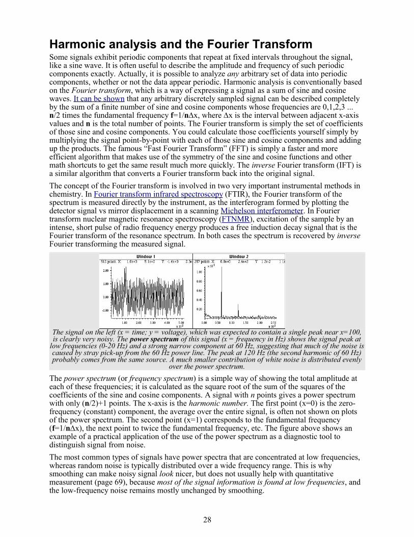
Harmonic analysis and the Fourier TransformSome signals exhibit periodic components that repeat at fixed intervals throughout the signal, like a sine wave. It is often useful to describe the amplitude and frequency of such periodic components exactly. Actually, it is possible to analyze any arbitrary set of data into periodic components, whether or not the data appear periodic. Harmonic analysis is conventionally based on the Fourier transform, which is a way of expressing a signal as a sum of sine and cosine waves. It can be shown that any arbitrary discretely sampled signal can be described completely by the sum of a finite number of sine and cosine components whose frequencies are 0,1,2,3 ... n/2 times the fundamental frequency f=1/nDx, where Dx is the interval between adjacent x-axis values and n is the total number of points. The Fourier transform is simply the set of coefficients of those sine and cosine components. You could calculate those coefficients yourself simply by multiplying the signal point-by-point with each of those sine and cosine components and adding up the products. The famous “Fast Fourier Transform” (FFT) is simply a faster and more efficient algorithm that makes use of the symmetry of the sine and cosine functions and other math shortcuts to get the same result much more quickly. The inverse Fourier transform (IFT) is a similar algorithm that converts a Fourier transform back into the original signal.

The concept of the Fourier transform is involved in two very important instrumental methods in chemistry. In Fourier transform infrared spectroscopy (FTIR), the Fourier transform of the spectrum is measured directly by the instrument, as the interferogram formed by plotting the detector signal vs mirror displacement in a scanning Michelson interferometer. In Fourier transform nuclear magnetic resonance spectroscopy (FTNMR), excitation of the sample by an intense, short pulse of radio frequency energy produces a free induction decay signal that is the Fourier transform of the resonance spectrum. In both cases the spectrum is recovered by inverse Fourier transforming the measured signal.

The signal on the left (x = time; y = voltage), which was expected to contain a single peak near x=100, is clearly very noisy. The power spectrum of this signal (x = frequency in Hz) shows the signal peak at

low frequencies (0-20 Hz) and a strong narrow component at 60 Hz, suggesting that much of the noise is caused by stray pick-up from the 60 Hz power line. The peak at 120 Hz (the second harmonic of 60 Hz) probably comes from the same source. A much smaller contribution of white noise is distributed evenly

over the power spectrum.

The power spectrum (or frequency spectrum) is a simple way of showing the total amplitude at each of these frequencies; it is calculated as the square root of the sum of the squares of the coefficients of the sine and cosine components. A signal with n points gives a power spectrum with only (n/2)+1 points. The x-axis is the harmonic number. The first point (x=0) is the zero-frequency (constant) component, the average over the entire signal, is often not shown on plots of the power spectrum. The second point (x=1) corresponds to the fundamental frequency (f=1/nDx), the next point to twice the fundamental frequency, etc. The figure above shows an example of a practical application of the use of the power spectrum as a diagnostic tool to distinguish signal from noise.

The most common types of signals have power spectra that are concentrated at low frequencies, whereas random noise is typically distributed over a wide frequency range. This is why smoothing can make noisy signal look nicer, but does not usually help with quantitative measurement (page 69), because most of the signal information is found at low frequencies, and the low-frequency noise remains mostly unchanged by smoothing.

28

The figures below show a classic example of harmonic analysis: the annual variation in the number of observed sunspots, which have been recorded since the year 1700! In this case the

time axis is in years. A plot of the power spectrum (bottom window) shows a strong peak at 0.09 cycles/year. If the data are plotted (on the bottom right) with time on the x-axis, the plot more clearly shows the well-known 11-year sunspot cycle (plus some evidence of a weaker cycle at around a 100-year period). These power spectra were plotted with iSignal (see page 85). The zeroth harmonic is not shown.

In the example illustrated on the right, the signal (in the top window) contains no visually evident periodic components; it seems to be only random noise. However, the frequency spectrum (in the bottom window) shows that there is much more to this signal than meets the eye. There are in fact two major frequency components: one at low frequencies around 0.02 and a stronger one at high frequencies between 0.5 and 5. (If the x-axis units of the signal plot is in seconds, the units of the frequency spectrum plot would be cycles per second; note that the x-axis is logarithmic). In this particular case, the lower frequency component is in fact the signal, and the higher frequency component is residual “blue” noise left over from previous signal processing. The two components are fortunately well separated on the frequency axis, suggesting that low-pass filtering (i.e. smoothing) will able to remove the noise without distorting the signal.

It is possible to compute the Fourier transform and power spectrum of any signal, such as an optical spectrum, where the independent variable might be wavelength or wavenumber, or an electrochemical signal, where the independent variable might be volts. The units of the x-axis of the power spectrum are simply the reciprocal of the units of the x-axis of the original signal (e.g. nm-1 for a signal whose x-axis is in nm).

Harmonic analysis provides another way to understand signal-to-noise ratio, filtering, smoothing, and differentiation. Smoothing (page 11) is a form of low-pass filtering, reducing the high-frequency components of a signal. If a signal consists of smooth features, such as Gaussian peaks, then its power spectrum will be concentrated at low frequencies. If that signal is con-taminated with white noise (spread out evenly over all frequencies), then smoothing will make the signal look better, because it reduces the high-frequency components of the noise. However, the low-frequency noise will remain in the signal after smoothing, where it will continue to interfere with the measurement of signal parameters such as peak heights, positions, widths, and areas. This can be demonstrated by least-squares measurement (page 69).

Conversely, differentiation (page 17) is a form of high-pass filtering, reducing the low frequency components of a signal and emphasizing any high-frequency components in the signal. As successive orders of differentiation are applied, the frequency spectrum shifts progressively to higher frequencies. So the optimum range for signal information of a differentiated signal is

29

restricted to an intermediate frequency range, with little useful information above and below that range. Real experimental signals are often contaminated with drift and baseline shift, which are essentially low-frequency effects, and with random noise, which is usually spread out over all frequencies. For these reasons, differentiation is always used in conjunction with smoothing. Working together, they act as a kind of frequency-selective bandpass filter that optimally passes the band of frequencies containing the signal information but reduces both the lower-frequency drift and background, as well as the high-frequency noise. SPECTRUM includes a power spectrum function and forward and reverse Fourier transforms. Matlab and Octave have built-in functions for computing the Fast Fourier Transform and its inverse (FFT and IFFT). A “Slow Fourier Transform” function has also been published. iSignal version 2.8 (page 86) has a Frequency Spectrum mode, toggled on and off by the Shift-S key, which computes the frequency spectrum of the segment of the signal isolated in the upper window and displays it in the lower window. Use the pan and zoom keys to adjust the region of the signal to be viewed. Press Shift-A to cycle through four plot modes (linear, semilog X, semilog Y, or log-log) and press Shift-X to toggle between a frequency on the x axis and time on the x-axis. The frequency (or time) and the harmonic number of the largest component of the spectrum is displayed on the left. All signal processing functions remain active in the frequency spectrum mode (smooth, derivative, etc) so you can observe the effect of these functions on the frequency spectrum of the signal. Press Shift-S again to return to the normal mode.

iPower is a keyboard-controlled Matlab interactive power spectrum demonstrator, useful for teaching and learning about the power spectra of different types of signals and the effect of signal duration and sampling rate. Single keystrokes allow you to select the type of signal (12 different signals included), the total duration of the signal, the sampling rate, and the global variables “f1” and “f2” which are used in different ways in the different signals. When the Enter key is pressed, the signal (y) is sent to the Windows WAVE audio device. Press K to see a list of all the keyboard commands. Tested in Matlab version 7.8 (R2009a). See http://tinyurl.com/cey8rwh.

KEYBOARD CONTROLS: Adjust signal duration 10% up/down.........A,Z Adjust sampling rate 10% up/down...........S,X Adjust first variable 10% up/down......... D,C Adjust second variable 10% up/down........ F,V Cycle through Linear/Log plot modes..........L Switch X-axis scale of power spectrum........H Print keyboard commands......................K Play signal as sound................Enter or P

SIGNAL TYPES, selected by the top row of keys from ` to Backspace:

Sine wave of frequency F1 (Hz) and phase F2........................ ` Square wave of frequency F1 (Hz) and phase F2....................... 1 Sawtooth wave of frequency F1(Hz)................................... 2 Triangle wave of frequency F1 (Hz) and phase F2..................... 3 Sine wave burst of frequency F1 (Hz)and length F2................... 4 440 Hz carrier amplitude modulated by sine wave..................... 5 440 Hz carrier frequency modulated by sine wave..................... 6 Sine wave of frequency F1 (Hz) modulated with Gaussian.............. 7 Sine wave of frequency F1 (Hz) with non-linear transfer function ... 8 Sine wave sweep from 0 to f1 (Hz)................................... 9 Sine wave of plus random white noise................................ 0 Pink (1/f) noise.................................................... - Sine wave of frequency F1 (Hz) and amplitude F2 plus pink noise..... = Used-defined signal waveform........................................Backspace

Note: you can change the user-defined waveform, selected by the Backspace key, by editing lines 256 and 257 to any other expression of y=f(x) using f1 and f2 as adjustable parameters.

30

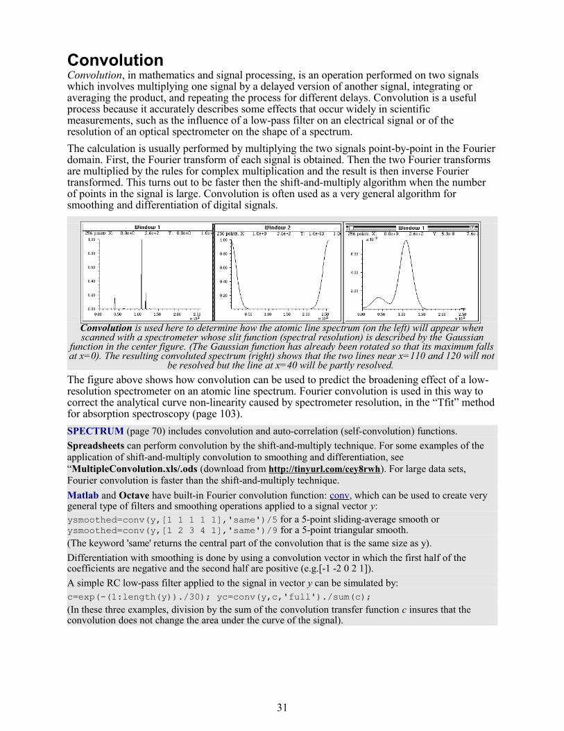
ConvolutionConvolution, in mathematics and signal processing, is an operation performed on two signals which involves multiplying one signal by a delayed version of another signal, integrating or averaging the product, and repeating the process for different delays. Convolution is a useful process because it accurately describes some effects that occur widely in scientific measurements, such as the influence of a low-pass filter on an electrical signal or of the resolution of an optical spectrometer on the shape of a spectrum.

The calculation is usually performed by multiplying the two signals point-by-point in the Fourier domain. First, the Fourier transform of each signal is obtained. Then the two Fourier transforms are multiplied by the rules for complex multiplication and the result is then inverse Fourier transformed. This turns out to be faster then the shift-and-multiply algorithm when the number of points in the signal is large. Convolution is often used as a very general algorithm for smoothing and differentiation of digital signals.

Convolution is used here to determine how the atomic line spectrum (on the left) will appear when scanned with a spectrometer whose slit function (spectral resolution) is described by the Gaussian

function in the center figure. (The Gaussian function has already been rotated so that its maximum falls at x=0). The resulting convoluted spectrum (right) shows that the two lines near x=110 and 120 will not

be resolved but the line at x=40 will be partly resolved.

The figure above shows how convolution can be used to predict the broadening effect of a low-resolution spectrometer on an atomic line spectrum. Fourier convolution is used in this way to correct the analytical curve non-linearity caused by spectrometer resolution, in the “Tfit” method for absorption spectroscopy (page 103).

SPECTRUM (page 70) includes convolution and auto-correlation (self-convolution) functions.

Spreadsheets can perform convolution by the shift-and-multiply technique. For some examples of the application of shift-and-multiply convolution to smoothing and differentiation, see “MultipleConvolution.xls/.ods (download from http://tinyurl.com/cey8rwh). For large data sets, Fourier convolution is faster than the shift-and-multiply technique.

Matlab and Octave have built-in Fourier convolution function: conv, which can be used to create very general type of filters and smoothing operations applied to a signal vector y: ysmoothed=conv(y,[1 1 1 1 1],'same')/5 for a 5-point sliding-average smooth or ysmoothed=conv(y,[1 2 3 4 1],'same')/9 for a 5-point triangular smooth. (The keyword 'same' returns the central part of the convolution that is the same size as y).

Differentiation with smoothing is done by using a convolution vector in which the first half of the coefficients are negative and the second half are positive (e.g.[-1 -2 0 2 1]).

A simple RC low-pass filter applied to the signal in vector y can be simulated by: c=exp(-(1:length(y))./30); yc=conv(y,c,'full')./sum(c); (In these three examples, division by the sum of the convolution transfer function c insures that the convolution does not change the area under the curve of the signal).

31

DeconvolutionDeconvolution is the converse of convolution in the sense that division is the converse of multiplication*. In fact, the deconvolution of one signal from another is usually performed by point-by-point division of the two signals in the Fourier domain**, that is, dividing the Fourier transforms of the two signals and then inverse-transforming the result.

The practical significance of deconvolution is that it can be used as an artificial (i.e. compu-Ztational) way to reverse the result of a convolution occurring in the physical domain, for example, to reverse the signal distortion effect of an electrical filter or of the finite resolution of a spectrometer. Two different examples of the application of deconvolution are shown in the two figures on this page

Deconvolution is used here to remove the distorting influence of an exponential tailing transfer function from a recorded signal (Window 1, left) that is the result of an unavoidable RC low-pass filter action in the electronics. The transfer function (Window 2, center) is usually either calculated on the basis of some theoretical model or is measured experimentally as the output signal produced by applying an impulse (delta) function to the input of the system. The response function, with its maximum at x=0, is deconvoluted from the original signal . The result (right) shows a closer approximation to the real shape of the peaks; however, the signal-to-noise ratio is unavoidably degraded.

A different application of the deconvolution function is to reveal the nature of an unknown data trans-formation function that has been applied to a data set by the measurement instrument itself. In this example, the first signal (from left to right) is a uv-visible absorption spectrum recorded from a commercial photodiode array spectrometer (X-axis: nanometers; Y-axis: milliabsorbance). The second signal is the first derivative of this spectrum produced by an (unknown) algorithm in the software supplied with the spectrometer. The objective here is to understand the nature of the differentiation/ smoothing algorithm that the instrument's software uses. The third signal is the result of deconvoluting the derivative spectrum (top right) from the original spectrum (top left). This therefore must be the convolution function used by that differentiation algorithm. Shifting and expanding it on the x-axis makes the function easier to see (last signal). Expressed in terms of the smallest whole numbers, the convolution series is seen to be +2, +1, 0, -1, -2. This simple example of “reverse engineering” would make it possible to compare results from other instruments or to duplicate these result on other equipment.

When applying deconvolution to experimental data, to remove the effect of a known broadening or low-pass filter operator caused by the experimental system, a very serious signal-to-noise degradation commonly occurs. Any noise added to the signal by the system after the convolution by the broadening or low-pass filter operator will be greatly amplified when the Fourier transform of the signal is divided by the Fourier transform of the broadening operator, because the high frequency components of the broadening operator (the denominator in the division of the Fourier transforms) are typically very small, resulting in a great amplification of high frequency noise in the resulting deconvoluted signal. (See the Matlab/Octave code example at

32

the bottom of this page). This can be controlled but not completely eliminated by smoothing and by constraining the deconvolution to a frequency region where the signal has a sufficiently high signal-to-noise ratio. You can see this noise amplification happening in the example in the first example above. However, this is not observed in the example in the second example, because in that case the noise is introduced before the convolution by the differentiation; high frequency components of the denominator in the division of the Fourier transforms are typically much larger, and the only additional noise comes from numerical round-off errors in the computations, which are almost always much smaller than the noise in the experimental signals.

Note: The term “deconvolution” is sometimes also used for the process of resolving or decomposing a set of overlapping peaks into their separate components, usually by the technique of iterative least-squares curve fitting (page 54) of a peak model to the data set. The process is actually conceptually distinct from Fourier deconvolution discussed here, because in deconvolution the underlying peak shape is unknown but the broadening function is assumed to be known; whereas in iterative least-squares curve fitting the underlying peak shape is assumed to be known but the broadening function is unknown. * If you know that mx equals n, where m and n are known but x is unknown, then x equals n/m. Conversely if you know that m convoluted with x equals n, where m and n are known but x is unknown, then x equals m deconvoluted from n.

** Fourier transforms are usually expressed in terms of complex numbers, with real and imaginary parts. If the Fourier transform of the first signal is a + ib, and the Fourier transform of the second signal is c + id, then the ratio of the two Fourier transforms is

by the rules for the division of complex numbers.

SPECTRUM (page 70) includes a Fourier deconvolution function.

Matlab and Octave have a built-in function for Fourier deconvolution: deconv. An example of its application is shown here. The vector yc (line 6) represents a noisy signal (y) that has been previously convoluted with a known transfer function c before being measured as yc. In line 7, c is deconvoluted from yc, to try to recover the original signal y before the convolution (as ydc). This works only if the transfer function c is known. Moreover, noise that is added after the convolution by the transfer function (line 6) will be significantly amplified in the recovered signal ydc.

x=0:.01:20;y=zeros(size(x)); % Start with 2000 zerosy(900:1100)=1; % Add a rectangular pulse 200 points widey=y+.01.*randn(size(y)); % Add some random noise before the convolutionc=exp(-(1:length(y))./30); % exponential trailing convolution functionyc=conv(y,c,'full')./sum(c); % Create exponential rectangular function ycyc=yc+.01.*randn(size(yc)); % Add some random noise after the convolutionydc=deconv(yc,c).*sum(c); % Deconvolute exponential function c from ycsubplot(2,2,1);plot(x,y);title('original y');subplot(2,2,2);plot(x,c);title('c')subplot(2,2,3);plot(x,yc(1:2001));title('yc');subplot(2,2,4);plot(x,ydc);title('recovered y')

33

Fourier filterThe Fourier filter is a type of filtering or smoothing function that is based on the frequency components of a signal. It works by taking the Fourier transform of the signal, manipulating the amplitudes of the frequency components, then inverse transforming the result. A simple example of the application of the Fourier filter is given in the figure below. In this case, the assumption is made that the frequency components of the signal fall predominantly at low frequencies and those of the noise fall predominantly at high frequencies, so all the frequency components above a certain limit are simply cut off (multiplied by zero). The cut-off frequency is adjusted so that it will allow most of the noise to be eliminated while not distorting the signal significantly.

The signal at the far left seems to be only random noise, but its power spectrum (Window 2, second from left) shows that high-frequency components dominate the signal. The power spectrum is expanded in the X and Y directions to show more clearly the low-frequency region (Window 1, right). Working on the hypothesis that the components above the 20th harmonic are noise, simple Fourier cut-off function can be used to delete the higher harmonics and to reconstruct the signal from the first 20 harmonics. The result (far right) shows the signal contains two bands at about x=200 and x=300 that were totally obscured by noise in the original signal.

SPECTRUM includes a simple Fourier low-pass filter function with adjustable harmonic cut-off. Matlab and Octave: FouFilter.m is a more flexible Fourier filter that can serve as a low-pass, high-pass, band-pass, or band-reject (notch) filter with variable cut-off rate. It has the form:

ry=FouFilter(y,samplingtime,centerfrequency,frequencywidth,shape,mode)

where y is the time-series signal vector, 'samplingtime' is the total duration of sampled signal in seconds, milliseconds, or microseconds; 'centerfrequency' and 'frequencywidth' are the center frequency and width of the filter in Hz, KHz, or MHz, respectively; 'Shape' determines the sharpness of the cut-off. If shape = 1, the filter is Gaussian; as shape increases the filter shape becomes more and more rectangular. Set mode = 0 for bandpass filter, mode = 1 for band-reject (notch) filter. FouFilter returns the filtered signal in ry. It can handle signals of virtually any length, limited only by the memory in your computer.

Example: plot(FouFilter(tan(1:1000),19,2,2,0))

iFilter, an Interactive Fourier Filter for Matlab shown on the right, allows you to adjust the Fourier filter parameters (center frequency, filter width, and cut-off rate) while observing the effect on the signal output dynamically. This is a self-contained Matlab function that does not require any toolboxes or add-on functions.

Download any of these functions from http://tinyurl.com/cey8rwh.

See http://terpconnect.umd.edu/~toh/spectrum/InteractiveFourierFilter.htm for instructions.

34

Integration and peak area measurement The symbolic integration of functions and the calculation of definite integrals are topics that are introduced in elementary Calculus courses. The numerical integration of digitized signals finds application in analytical signal processing mainly as a method for measuring the areas under the curves of peak-type signals. Peak area measurements are very important in chromatography. Quantitative measurement in chromatography is customarily carried out on the basis of peak area rather than peak height measurement, because peak area is less sensitive to the influence of peak broadening (dispersion) mechanisms. These broadening effects, which arise from many sources, cause chromatographic peaks to become shorter, broader, and more unsymmetrical, but they have little effect on the total area under the peak. If the detector response is linear, the peak area remains proportional to the total quantity of substance passing into the detector. For this reason peak area measurements are often found to be more reliable than peak height measurement.

The simple numeric integration of a digital, for example by Simpson's rule, will convert a series of peaks into a series of steps, the height of each of which is proportional to the area under that peak. This is a commonly used method in proton NMR spectroscopy, where the area under each peak or multiplet is proportional to the number of equivalent hydrogen atoms responsible for that peak. But this works well only if the peaks are well separated from each other.

In chromatographic analysis there is often the problem of measuring the area under the curve of the peaks when they are not well resolved or are superimposed on a background. For example, the figure below shows a series of four computer-synthesized Gaussian peaks that all have the same height, width, and area, but the separation between the peaks on the right is insufficient to achieve complete resolution.

Peak area measurement for overlapping peaks, using the perpendicular drop method.

The classical way to handle this problem is to draw two vertical lines from the left and right bounds of the peak down to the x-axis and then to measure the total area bounded by the signal curve, the x-axis (y=0 line), and the two vertical lines. This is often called the perpendicular drop method; it's an easy task for a computer, although tedious to do by hand. The idea is illustrated for the second peak from the left in the figure. The left and right bounds of the peak are usually taken as the valleys (minima) between the peaks or as the point half-way between the peak center and the centers of the peaks to the left and right. Using this method it is possible to estimate the area of the second peak to an accuracy of about 0.3% and the second and third peak to an accuracy of better than 4%.

However, that simple method works well only if the peaks are symmetrical, not very different in height, and not too highly overlapped (as is the case for the first two peaks in this example). In the special case where a peak is superimposed on a broader curved baseline, one can use the tangent skim method, in which a linear baseline is interpolated between the tangent points on both sides of the peak and subtracted. But in general, the most accurate way to measure the area of overlapping peaks is to use some type of least-squares curve fitting, discussed on pages 37-69. If the peak shapes, positions, and widths are known beforehand, and only the peak amplitudes are unknown, the method of multiple linear regression can be used (page 49). If the peak

35

positions, widths, and amplitudes are unknown, and only the fundamental peak shapes are known, then the iterative least-squares method can be employed (page 54). In any case, the peak shape must be known in order to use least-squares curve fitting methods.Software details.Matlab and Octave have built-in commands for the sum of elements (“sum”, “cumsum”), trapezoidal numerical integration (“trapz”), and adaptive Simpson quadrature (“quad”). For example:>> x=-5:.1:5; y=exp(-(x).^2);trapz(x,y)

accurately computes the area under the curve of an isolated Gaussian, which is theoretically predicted to be the square root of p (that is, 1.7725). By itself, however, these simple functions do not solve the problem of measuring areas of overlapping peaks or peaks superimposed on a background signal.

iSignal (page 85) performs several of the signal processing functions described in this tutorial, including measurement of peak area using Simpson's Rule and the perpendicular drop and tangent skim methods. It can also subtract the baseline from a series of peaks using a manual piecewise-linear approximation.

The figure on the left shows a Matlab/Octave experiment that creates a signal containing 5 peaks with the same peak areas but broadened by increasing degrees of exponential

broadening, similar to the broadening of peaks commonly encountered in chromatography:>> x=5:.1:65;>> y=modelpeaks2(x,[1 5 5 5 5],[1 1 1 1 1],[10 20 30 40 50],[3 3 3 3 3],...[0 -5 -10 -15 -20]);>> plot(x,y)To use iSignal to measure the areas of each of these peaks by the perpendicular drop method, use the pan and zoom keys to position the two outer cursor lines (dotted magenta lines) in the valley on either side of each peak. The area is displayed below the upper window. The peak heights are different but the areas are almost exactly the same; this is why peak areas are better than peak heights in chromatography.

The functions peakfit.m (page 90) and ipf.m (page 95) also measure peak area of the best-fit overlapping-peak models; a practical chromatography example is given on page 96. The following code generates four Gaussian peaks, just like the figure on page 35, all with the same height, width, and area, and measures it with peakfit.m:>> x=[0:.01:18];>> y=exp(-(x-4).^2)+exp(-(x-9).^2)+exp(-(x-12).^2)+exp(-(x-13.7).^2);>> peakfit([x;y],9,18,4,1,0,10,0,0,0)

iPeak (page 74) can also be used to estimate peak areas. It uses the same Gaussian curve fitting method as iSignal, and it has the advantage that it can detect and measure all the peaks in a signal in one operation, but the areas are accurate only if the peaks are Gaussian and well separated. In general, the most accurate peak area measurements can be made with iterative least-squares peak fitting (page 54), for example using peakfit.m or ipf.m (page 90, 95, 96). In all of these methods, the presence of a background signal on which the peaks are superimposed will greatly influence the measured peak area if not corrected or compensated. iSignal, iPeak, and peakfit all have four automatic baseline correction modes (page 62), and iSignal and iPeak have a multipoint piecewise linear background subtraction function (page 86). See http://tinyurl.com/cey8rwh.

For gas chromatography and mass spectrometry specifically, I recommend Philip Wenig's OpenChrom software, shown on the left, an open source data system that can import binary and textual chromatographic data files directly in several common formats. It includes methods to detect baselines and peaks and to integrate peaks in a chromatogram, and it can be set to ignore specific mass fragments (m/z) such as nitrogen (28) or water (18). Extensive documentation is available. It is available for Windows, Linux, Solaris and Mac OS X.

36

Curve fitting A: Linear Least SquaresThe objective of curve fitting is to find the parameters of a mathematical model that describes a set of (usually noisy) data in a way that minimizes the difference between the model and the data. The most common approach is the “linear least squares” method, also called “polynomial least squares”, a well-known mathematical procedure for finding the coefficients of polynomial equations that are a “best fit” to a set of X,Y data. A polynomial equation expresses the dependent variable Y as a polynomial in the independent variable X, for example as a straight line (Y = a + bX, where a is the intercept and b is the slope), or a quadratic (Y = a + bX + cX2), or a cubic (Y = a + bX + cX2 + dX3), or higher-order polynomial. Those coefficients (a, b, c, etc) can be used to predict values of Y for each X. “Best fit” simply means that the squares of the differences between the actual measured Y values and the Y values predicted by that equation are minimized.

In all these cases, Y is a linear function of the parameters a,b,c, etc. This is why we call it a “linear” least-squares fit, not because the plot of X vs Y is linear. Only for the first-order polynomial is the plot of X vs Y linear.

Least-squares fits can be calculated by some hand-held calculators and smartphones, by spreadsheets, and by dedicated computer programs (see page 46 for details). Although it is possible to estimate the best-fit straight line by visual estimation and a straightedge, the least-squares method is more objective and easier to automate. (If you were to give a set of data to five different people and ask them to estimate the best-fit line visually, you'd get five slightly different answers, but it you gave that data set to five different computer programs, you'd get the exact same answer every time).

Here's a very simple example: the historical prices of different sizes of SD memory cards advertised in the February 19, 2012, issue of the New York Times.

Memory Capacity in GBytes

Price in US dollars

2 $9.99

4 $10.99

8 $19.99

16 $29.99

What's the relationship between memory capacity and cost? Of course, we expect that the larger-capacity cards should cost more than the smaller-capacity ones, and if we plot cost vs capacity (graph on the right), we can see a rough straight-line relationship. Using a linear least-squares calculation, where X = capacity and Y = cost, the straight-line equation that most simply describes these data (rounding to the nearest penny) is: Cost = $6.56 + Capacity * $1.49 So, 1.49 is the slope (b) and 6.56 is the intercept (a). (The equation is plotted as the solid line that passes among the data points in the figure). Basically, this is saying that the cost of a memory card consists of a fixed cost of $6.56 plus $1.49 for each Gbyte of capacity. How can we interpret this? The $6.56 represents the costs that are the same regardless of the memory capacity: a reasonable guess is that it includes things like

37

packaging (the different cards are the same physical size and are packaged the same way), shipping, marketing, advertising, and retail shop shelf space. The $1.49 (actually 1.49 dollars/Gbyte) represents the increasing retail price of the larger integrated circuit chips inside the larger capacity cards, primarily because they have more value for the consumer but also may cost more to make because they use more silicon, are more complex, and have a higher chip-testing rejection rate in the production line. So in this case the slope and intercept have real physical and economic meanings.

What can we do with this information? First, we can see how closely the actual prices conform to this equation: pretty well but not perfectly. The line of the equation passes among the data points but does not go exactly through each one. That's because actual retail prices are also influenced by several factors that are unpredictable and random: local competition, supply, demand, and even rounding to the nearest “neat” number; all those factors constitute the “noise” in these data. The least squares procedure also calculates R2, called the coefficient of determination or the correlation coefficient, which is an indicator of the “goodness of fit”. R2 is exactly 1.0000 when the fit is perfect, less than that when the fit is imperfect. The closer to 1.0000 the better. An R2 value of 0.99 means a fairly good fit; 0.999 is a very good fit.

The second way we can use these data is to predict the likely prices of other card capacities, if they were available, by putting in the capacity into the equation and evaluating the cost. For example, a 12 Gbyte card would be expected to cost $24.44 according to this model. And a 32 Gbyte card would be predicted to cost $54.29, but beware, that would be predicting beyond the range of the available data. That's called “extrapolation”- and it's very risky because you don't really know what other factors may influence the data beyond the last data point. You could also solve the equation for capacity as a function of cost and use it to predict how much capacity could be expected to be bought for a given amount of money (if such a product were available).

Here's another related example: the historical prices of flat-screen LCD TVs as a function of screen size, as they were advertised on the Web in 2012. The prices of five selected models, similar except for screen size, are plotted against the screen size in inches, in the figure on the left, and are fit to a first-order (straight-line) model. As for the previous example, the fit is not perfect. The equation of the best-fit model is shown at the top of the graph, along with the R2

value (0.9649) indicating that the fit is not particularly good. (Worse, you can see from the best-fit line that a 40 inch set would be predicted to have a negative cost! They would pay you to take these sets? I don't think so. Clearly something is wrong here).

The goodness of fit is shown even more clearly in the little graph at the bottom of the figure, with the red dots, which shows the “residuals” - the differences between each data point and the least-squares fit at that point. You can see that the deviations from zero are fairly large (±10%), but more important, they are not completely random; they form a clearly visible U-shaped curve. This is a tip-off that the straight-line model we have used here may not be ideal and that we might get a better fit with another model. (Or it might be just chance: the first and last points might be higher than expected because those were unusually expensive TVs for those sizes. How would you really know for sure, unless your data collection was very careful?).

38

Least-squares calculations can fit not only straight-line data, but any set of data that can be described by a polynomial, for example a second-order (quadratic) equation (Y = a + bX + cX2). Applying a second-order (“quadratic”) fit to these data, we get the graph on the right. Now the R2

value is higher, 0.9985, indicating that the fit is much better (but again not perfect), and also the residuals (the red dots at the bottom) are smaller and more random.

The observation that a quadratic fits the data better is not really surprising, because the size of a TV screen is quoted as the length of the diagonal (from one corner of the screen to its opposite corner), but the quantity of material, the difficulty of manufacture, the weight, and the power supply requirements of the screen should all scale with the screen area. Area is proportional to the square of the linear measure, so the inclusion of an X2 term in the model is quite reasonable in this case. With this quadratic fit, the 40 inch set would be predicted to cost under $500, which is more sensible than the linear fit. In this case a quadratic (rather than linear) model is justified not simply because it fits the data better, but because it is expected in principal on the basis of the relationship between length and area.

The graph on the left shows a third example, taken from analytical chemistry: a straight-line calibration data set where X = concentration and Y = instrument reading (Y = a + bX). (If you are viewing this on-line, click to download that data). The blue dots are the data points. They don't all fall in a perfect straight line because of random noise and measurement error in the instrument readings and possibly also volumetric errors in the concentrations of the standards (which are usually prepared in the laboratory by diluting a stock solution). For this set of data, the measured slope is 9.7926 and the intercept is 0.199.

In analytical chemistry, the slope of the calibration curve is often called the “sensitivity”. The intercept indicates the instrument reading that would be expected if the concentration were zero. Ordinarily instruments are adjusted (“zeroed”) by the operator to give a reading of zero for a concentration of zero, but random noise and instrument drift can cause the intercept to be non-zero for any particular calibration set. In fact, this data set is computer-generated; the “true” value of the slope was exactly 10 and of the intercept was exactly zero before noise was added, and the noise was added by a random-number generator with zero mean. So in this case the presence of the noise caused this particular measurement of slope to be off by about 2%. Had there been a larger number of points in this data set, the calculated values of slope and intercept would almost certainly have been better. (On average, the accuracy of measurements of slope and intercept improve with the square root of the number of points in the data set).

Once the calibration curve is established, it can be used to determine the concentrations of unknown samples that are measured on the same instrument, for example by solving the equation for concentration as a function of instrument reading. The concentration and the instrument readings can be recorded in any convenient units, as long as the same units are used for calibration and for the measurement of unknowns.

A plot of the “residuals” for the calibration data (below, left) shows results that are questionable; they don't seem to be particularly random. Except for the 6th data point (at a

39

concentration of 0.6), the other points seem to form a rough U-shaped curve, indicating that a quadratic equation might be a better model for those points that a straight line. Can we reject the 6th point as being an “outlier”, perhaps caused by a mistake in preparing that solution standard or in reading the

instrument for that point? The only way to know for sure is to repeat that standard solution preparation and calibration and see if that U shape persists in the residuals. Many instruments do give a very linear calibration response, but others show a slightly non-linear response under some circumstances. But in fact, the calibration data used for this particular example were computer-generated to be perfectly linear, with normally-distributed random numbers added to simulated noise. So in fact that 6th point is really not an outlier and the curve is not non-linear, but you would not know that in a real application. It would have been a mistake to discard that 6th point and use a quadratic fit. Moral: don't throw out data points just because they seem a little off, unless you have good reason, and don't use higher-order polynomial fits just to get better fits if the instrument is known to give linear response under those circumstances. Even perfect normally-distributed random errors can occasionally give individual deviations that are quite far from the average and might tempt you into thinking that they are outliers.

Reliability of curve fitting resultsHow reliable are the slope, intercept and other polynomial coefficients obtained from least-squares calculations on experimental data? The single most important factor is the appropriateness of the model chosen; it's critical that the model (e.g. linear, quadratic, etc) be a good match to the actual underlying shape of the data. You can do that either by choosing a model based on the known and expected behavior of that system (like using a linear calibration model for an instrument that is known to give linear response under those conditions) or by choosing a model that always gives randomly-scattered residuals that do not exhibit a regular shape. But even with a perfect model, the least-squares procedure applied to repetitive sets of measurements will not give the same results every time because of random error (“noise”) in the data. If you were to repeat the entire set of measurements many times and do least-squares calculations on each data set, the standard deviations of the coefficients would vary directly with the standard deviation of the noise and inversely with the square root of the number of data points in each fit, all else being equal. The problem, obviously, is that it is not always possible to repeat the entire set of measurements many times. You may have only one set of measurements, and each experiment may be very expensive to repeat. So, it would be good to have some sort of short-cut method that would predict the standard deviations of the coefficients without actually repeating the measurements. Here I will describe three general ways to predict the standard deviations of the polynomial coefficients.

Algebraic Propagation of errors. The classical way is based on the rules for mathematical error propagation. The propagation of errors of the entire curve-fitting method can be described in closed-form algebra by breaking down the method into a series of simple differences, sums, products, and ratios, and applying those rules to each step. The result of this procedure for a first-order (straight line) least-squares fit are shown in the last two lines of the set of equations on page 46. Essentially, these equations make use of the deviations from the least-squares line (the “residuals”) to estimate the standard deviations of the slope and intercept, based on the assumption that the deviations in that single data set are random and representative of the deviations that would be obtained upon repeated measurements. Because these predictions are based only on a single data set, they are good only insofar as that data set is typical of others that might be obtained in repeated measurements. If your random deviations happen to be small when you acquire your data set, you'll get a deceptively good-looking fit, but then your estimates of the standard deviation of the slope and intercept will be too low, on average. If your random deviations happen to be large in that data set, you'll get a deceptively bad-looking fit, but then your estimates of the standard deviation will be too high, on average. This problem becomes worse when the number of data points is small. This is not to say that it is not worth the trouble

40

to calculate the predicted standard deviations of slope and intercept, but keep in mind that these predictions are accurate only if the number of data points is large (and only if the deviations are random and normally distributed).

Monte Carlo simulation. Another way of estimating the standard deviations of the least-squares coefficients is to perform a random-number simulation (a type of Monte Carlo simulation). This requires that you know (by previous measurements) the average standard deviation of the random noise in the data. Using a computer, you construct a model of your data over the normal range of X and Y values (for example Y = intercept + slope*X + noise, where noise is the noise in the data), compute the slope and intercept of each simulated noisy data set, then repeat that process many times (usually a few thousand) with different sets of random noise, and finally compute the standard deviation of all the resulting slopes and intercepts. This is ordinarily done with normally-distributed random white noise, using the RANDN function that many programing languages have. If the model is good and the noise is white and well-characterized, the results will be a very good estimate of the expected standard deviations of the least-squares coefficients. (If the noise is is not white or is not constant, but rather varies with the X or Y values, or if the data have been smoothed, then that must be included in the simulation).

Obviously this method requires a computer and prior knowledge of the noise, and it is not so convenient as evaluating a simple algebraic expression. But there are two important advantages to this method: (1) is has great generality; it can be applied to curve fitting methods that are too complicated for the classical closed-form algebraic propagation of error calculations, even iterative non-linear methods; and (2) its predictions are based on the average noise in the data, not the noise in just a single data set. For that reason, it gives more reliable estimations, particularly when the number of data points in each data set is small. Nevertheless, you can not

41

always apply this method because you don't always know the average standard deviation or the frequency distribution of the noise in the data.

A Matlab/Octave script that compares the Monte Carlo simulation to the algebraic method above can be downloaded (LinearFiMC.m, from http://tinyurl.com/cey8rwh. By running this script with different sizes of data sets (NumPoints in line 10), you can see that the standard deviation predicted by the algebraic method fluctuates a lot from run to run when NumPoints is small (e.g. 10), but the Monte Carlo predictions are much more steady. When NumPoints is large (e.g. 1000), both methods agree very well.

The Bootstrap. The third method is the “bootstrap”, a procedure that involves choosing random data points with replacement from a single data set and analyzing each data set the same way (e.g. by a least-squares fit). Every data point is returned to the data set after sampling, so that (a) a particular data point from the original data set could appear multiple times in a given sample, and (b) the number of elements in each bootstrap sub-sample equals the number of elements in the original data set. As a simple example, consider a data set with 10 x,y pairs assigned the letters a through j. The original data set is represented as [a b c d e f g h i j], and some typical bootstrap sub-samples might be [a b b d e f f h i i] or [a a c c e f g g i j], each bootstrap sample containing the same number of data points, but with about half of the data pairs skipped and the others duplicated.

You would use a computer to generate hundreds or thousands of bootstrap samples like that and apply the calculation procedure under investigation (in this case a linear least-squares, but it could be any calculation) to each set. If there were no noise in the data set, and if the model were perfectly chosen, then all the points in the original data set and in all the bootstrap sub-samples would fall exactly on the model line, and the least-squares results would be the same for every sub-sample. But if there is noise in the data set, each bootstrap sample would give a slightly different result (e.g. the least-squares polynomial coefficients), because each one has a different subset of the random noise. The greater the amount of random noise in the data set, the greater would be the range of results from the bootstrap sub-samples. This enables you to estimate the uncertainty of the quantity you are estimating, just as in the Monte-Carlo method above. The difference is that the Monte-Carlo method is based on the assumption that the noise is can be accurately simulated by a random-number generator on a computer (i.e. is random, normally distributed, and has a known standard deviation), whereas the bootstrap method uses the actual noise in the data set at hand, like the algebraic method, except that it does not need an algebraic solution of error propagation. The bootstrap method thus shares its generality with the Monte Carlo approach, but like the algebraic method is limited by the assumption that the noise in that (possibly small) single data set is unsmoothed and is representative of the noise that would be obtained upon repeated measurements. Bootstrap computations can be done in Matlab/Octave (page 48) or in spreadsheets.

The Matlab/Octave script TestLinearFit.m (which you can download from http://tinyurl.com/cey8rwh) compares all three of these methods (the algebraic method, Monte Carlo simulation, and the bootstrap method) for a 100-point first-order linear least-squares fit. Each method is repeated on different data sets with the same average slope, intercept, and random noise, then the standard deviations (SD) of the slopes (SDslope) and intercepts (SDint) were compiled:NumPoints = 100 SD Noise = 9.236 x-range = 30 Simulation Algebraic equation Bootstrap method SDslope SDint SDslope SDint SDslope SDintMean SD: 0.1140 4.1158 0.1133 4.4821 0.1096 4.0203SD of SDs: 0.0026 0.0927 0.0081 0.3185 0.0122 0.4552

On average, the mean standard deviations (“Mean SD”) of the three methods agree very well, but the algebraic and bootstrap methods fluctuate more than the Monte Carlo simulation each time this script is run (the “SD of the SDs” is higher), because those methods are based on the noise

42

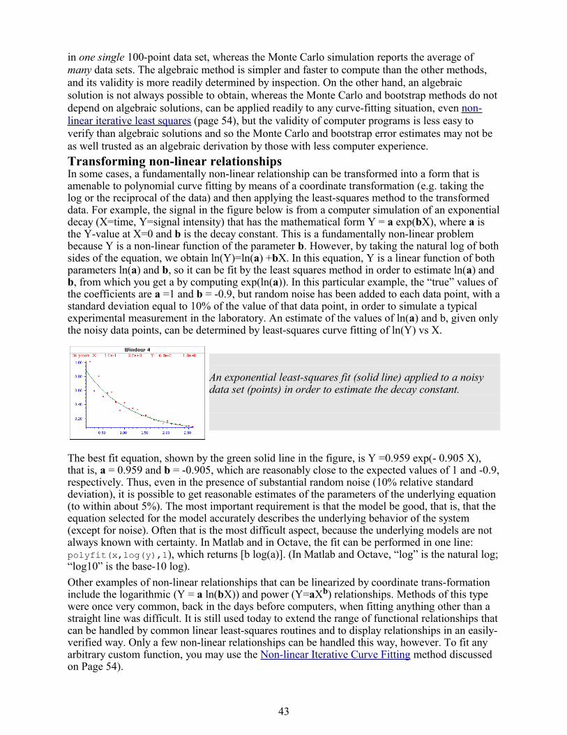
in one single 100-point data set, whereas the Monte Carlo simulation reports the average of many data sets. The algebraic method is simpler and faster to compute than the other methods, and its validity is more readily determined by inspection. On the other hand, an algebraic solution is not always possible to obtain, whereas the Monte Carlo and bootstrap methods do not depend on algebraic solutions, can be applied readily to any curve-fitting situation, even non-linear iterative least squares (page 54), but the validity of computer programs is less easy to verify than algebraic solutions and so the Monte Carlo and bootstrap error estimates may not be as well trusted as an algebraic derivation by those with less computer experience.

Transforming non-linear relationshipsIn some cases, a fundamentally non-linear relationship can be transformed into a form that is amenable to polynomial curve fitting by means of a coordinate transformation (e.g. taking the log or the reciprocal of the data) and then applying the least-squares method to the transformed data. For example, the signal in the figure below is from a computer simulation of an exponential decay (X=time, Y=signal intensity) that has the mathematical form Y = a exp(bX), where a is the Y-value at X=0 and b is the decay constant. This is a fundamentally non-linear problem because Y is a non-linear function of the parameter b. However, by taking the natural log of both sides of the equation, we obtain ln(Y)=ln(a) +bX. In this equation, Y is a linear function of both parameters ln(a) and b, so it can be fit by the least squares method in order to estimate ln(a) and b, from which you get a by computing exp(ln(a)). In this particular example, the “true” values of the coefficients are a =1 and b = -0.9, but random noise has been added to each data point, with a standard deviation equal to 10% of the value of that data point, in order to simulate a typical experimental measurement in the laboratory. An estimate of the values of ln(a) and b, given only the noisy data points, can be determined by least-squares curve fitting of ln(Y) vs X.

An exponential least-squares fit (solid line) applied to a noisy data set (points) in order to estimate the decay constant.

The best fit equation, shown by the green solid line in the figure, is Y =0.959 exp(- 0.905 X), that is, a = 0.959 and b = -0.905, which are reasonably close to the expected values of 1 and -0.9, respectively. Thus, even in the presence of substantial random noise (10% relative standard deviation), it is possible to get reasonable estimates of the parameters of the underlying equation (to within about 5%). The most important requirement is that the model be good, that is, that the equation selected for the model accurately describes the underlying behavior of the system (except for noise). Often that is the most difficult aspect, because the underlying models are not always known with certainty. In Matlab and in Octave, the fit can be performed in one line: polyfit(x,log(y),1), which returns [b log(a)]. (In Matlab and Octave, “log” is the natural log; “log10” is the base-10 log).

Other examples of non-linear relationships that can be linearized by coordinate trans-formation include the logarithmic (Y = a ln(bX)) and power (Y=aXb) relationships. Methods of this type were once very common, back in the days before computers, when fitting anything other than a straight line was difficult. It is still used today to extend the range of functional relationships that can be handled by common linear least-squares routines and to display relationships in an easily-verified way. Only a few non-linear relationships can be handled this way, however. To fit any arbitrary custom function, you may use the Non-linear Iterative Curve Fitting method discussed on Page 54).

43

Fitting Gaussian and Lorentzian peaks. A useful example of transformation to convert a non-linear relationship into a form that is amenable to polynomial curve fitting is the use of the natural log (ln) transformation to convert a Gaussian peak (y = h*exp(-((x-p)/(0.6005612*w)) ^2), where h is peak height, p is peak maximum position, and w is the full width at half maximum) into a quadratic (y = a + bx + cx2) that can be fit to the data by quadratic least squares. All three parameters of the Gaussian (h, p, and w) can be calculated from the three quadratic coefficients a, b, and c by solving 3 equations in 3 unknowns (for example, using Wolfram Alpha), resulting in h = exp(a-c*(b/(2*c))^2), p = -b/(2*c), and w = 2.35703/(sqrt(2)*sqrt(-c)). This is called “Caruana's algorithm”; see reference 46 on page 116.

One advantage of this type of Gaussian curve fitting, as opposed to simple visual estimation, is shown in the figure on the left, below. The signal is a Gaussian peak with a true peak height of 100 units, a true peak position of 100 units, and a true half-width of 100 units, but it is sparsely sampled only every 31 units on the x-axis. The resulting data set, shown by the red points in the upper left quadrant, has only 6 data points on the peak itself. If we were to take the maximum of those 6 points (the 3rd point from the left, with x=87, y=95) as the peak maximum, that would

not be very close to the true values of peak position (100) and peak height (100). If we were to take the distance between the 2nd the 5th data points as the peak width, we'd get 3*31=93, compared to the true value of 100.

However, taking the natural log of the data (upper right) produces a parabola that can be fit with a quadratic least-squares fit (shown by the blue line in the lower left). From the three coefficients of the quadratic fit we can calculate much more accurate values of the Gaussian peak parameters, shown at the

bottom of the figure (height=100.57; position=98.96; width=99.2). The plot in the lower right shows the resulting Gaussian fit (in blue) displayed with the original data (red points). The accuracy of those calculated peak parameters (about 1% in this example) is far better than the previous estimates and is limited only by the noise in the data. This figure was generated in Matlab/Octave, using the script “QuadFitToGaussian.m”. Note: in order for this method to work properly, the data set must not contain any zeros or negative points; if the signal-to-noise ratio is very poor, it may be useful to smooth the data slightly to prevent this problem. Moreover, the original Gaussian peak signal must have a zero baseline, that is, must tend to zero far from the peak center. In practice this means that any non-zero baseline must be subtracted from the data set before using this method.

A similar method can be derived for a Lorentzian peak, which has the form y=h/(1+((x-p)/(0.5*w))^2), by fitting a quadratic to the reciprocal of the y values. Just as for the Gaussian peak, all three parameters of the peak (height h, maximum position p, and width w) can be calculated from the three quadratic coefficients a, b, and c of the quadratic fit: h=4*a/((4*a*c)-b^2), p= -b/(2*a), and w= sqrt(((4*a*c)-b^2)/a)/sqrt(a), and the data set must not contain any zero or negative y values.

A more general approach to fitting peaks, which works for data sets with zeros and negative numbers and also for data with multiple overlapping peaks, is the non-linear iterative curve fitting method, discussed on Page 54.

But there is a downside to using coordinate transformation methods to convert non-linear relationships into simple polynomial form, and that is that the noise is also effected by the transformation, with the result that the propagation of error from the original data to the final results is often difficult to predict. For example, in the method just described for measuring the peak height, position, and width of Gaussian peaks, the results depends not only on the amplitude of noise in the signal, but also on how many points across the peak are taken for

44

fitting. In particular, as you take more points far from the peak center, where the y-values approach zero, the natural log of those points approaches negative infinity as y approaches zero. The result is that the noise of those low-magnitude points is unduly magnified and has a disproportional effect on the curve fitting. This runs counter the usual expectation that the quality of the parameters derived from curve fitting improves with the square root of the number of data points.

A reasonable compromise in this case is to take only the points in the top half of the peak, with Y-values down to one-half of the peak maximum. If you do that, the error propagation (predicted by a Monte Carlo simulation with constant normally-distributed random noise) shows that the relative standard deviations of the measured peak parameters are predicted by the following empirical expressions:

Relative standard deviation of the peak position =noise/sqrt(N),Relative standard deviation of the peak height = 1.73*noise/sqrt(N),Relative standard deviation of the peak width = 3.62*noise/sqrt(N),

where noise is the standard deviation of the noise in the data and N in the number of data points taken for the least-squares fit. You can see from these results that the measurement of peak position is most precise, followed by the peak height, with the peak width being the least precise. If one were to include points far from the peak maximum, where the signal-to-noise ratio is very low, the results would be poorer than predicted. These predictions depend on knowledge of the noise in the signal; if only a single sample of that noise is available for measurement,

there is no guarantee that sample is a representative sample, especially if the total number of points in the measured signal is small; the standard deviation of small samples is notoriously variable. Moreover, these predictions are based on a simulation with constant normally-distributed white noise; had the actual noise varied with signal level or with x-axis value, or if the probability distribution had been non-normal, those predictions would not necessarily have been accurate. The bootstrap method has the advantage that it samples the actual noise in the signal. You can download the Matlab/Octave code for this Monte Carlo simulation from http://tinyurl.com/cey8rwh. A similar simulation (GaussFitMC2.m) compares this method to fitting the entire Gaussian peak with the iterative method on pages 54 - 69, finding that the precision of the results is slightly better with the slower iterative method. Note 1: If you are viewing this document on-line, you can right-click on any of the m-file links above and select Save Link As... to download them for use within Matlab/Octave.

Note 2: In the curve fitting techniques described here and in the next two sections, there is no requirement that the x-axis interval between data points be uniform, as is the assumption in many of the other signal processing techniques previously covered. Curve fitting algorithms typically accept a set of arbitrarily-spaced x-axis values and a corresponding set of y-axis values.Note 3: It's important that the noisy signal not be smoothed before the least-squares calculations, because doing so will not improve the reliability of the least-squares results, but it will cause both the algebraic propagation-of-errors and the bootstrap calculations to seriously underestimate the standard deviation of the least-squares results. You can demonstrate using the most recent version of the script TestLinearFit.m by setting SmoothWidth in line 10 to something higher than 1, which will smooth the data before the least-squares calculations. This has no significant effect on the actual standard deviation as calculated by the Monte Carlo method, but causes the predicted standard deviation calculated by the algebraic propagation-of-errors and the bootstrap method to be much too low. (If the data are contaminated with large narrow spikes, it may be best to apply a median filter, page 15, before least-squares computations).

45

Math detailsThe least-squares best fit for an x,y data set can be computed using only basic arithmetic. Here are the relevant equations for computing the slope and intercept of the first-order best-fit equation, y = intercept + slope*x, , as well as the predicted standard deviation (SD) of the slope and intercept, and the coefficient of determination, “R2”, which is an indicator of the “goodness of fit”. ( R2 is 1.0000 if the fit is perfect and less than that if the fit is imperfect): n = number of x,y data points sumx = Σx sumy = Σy sumxy = Σx*y sumx2 = Σx*x meanx = sumx / n meany = sumy / n slope = (n*sumxy - sumx*sumy) / (n*sumx2 - sumx*sumx intercept = meany-(slope*meanx) ssy = Σ(y-meany)^2 ssr = Σ(y-intercept-slope*x)^2 R2 = 1-(ssr/ssy) SD of slope = SQRT(ssr/(n-2))*SQRT(n/(n*sumx2 - sumx*sumx)) SD of intercept = SQRT(ssr/(n-2))*SQRT(sumx2/(n*sumx2 - sumx*sumx)) (In these equations, Σ represents summation; for example, Σx means the sum of all the x values, and Σx*y means the sum of all the x*y products, etc).

The last two lines predict the standard deviation of the slope and intercept, based only on that data sample, assuming that the noise is normally distributed. These are estimates of the variability of slopes and intercepts you are likely to get if you repeated the data measurements over and over multiple times under the same conditions, assuming that the deviations from the straight line are due to random variability and not systematic error caused by non-linearity. If the deviations are random, they will be slightly different from time to time, causing the slope and intercept to vary from measurement to measurement, with a standard deviation predicted by these last two equations. However, if the deviations are caused by systematic non-linearity, they will be the same from from measurement to measurement, in which case the prediction of these last two equations will not be relevant, and you might be better off using a polynomial fit such as a quadratic or cubic. The reliability of these standard deviation estimates depends also on the number of data points n in the curve fit; they improve with the square root of n.

These calculations could be performed step-by-step by hand, with the aid of a calculator or a spreadsheet, with a program written in any programming language, a math Web page such as Wolfram Alpha (using the “linear fit” command), or with a Matlab / Octave script. A similar set of equations can be written to fit a second-order (quadratic or parabolic) equations to a set of data. The minimum number of data points required for a polynomial least-squares fit depends on the polynomial order: you need a minimum of two points for a first-order (straight-line) fit, a minimum of three points for a second-order (quadratic or parabolic) fit, a minimum of four points for a third-order (cubic) fit, etc, always one more than the polynomial order. With that minimum number of points, the fit will always be artificially perfect, no matter how large the errors in the data might be; so you get no hint of possible errors in the data because the best-fit line will always go right though all the points. The greater the number of points the better, because (a) you can see when there are errors in the data, and (b) because the errors have a greater changes of partially “canceling out” and resulting in a slope, intercept, and other coefficients that are closer to the true long-term average.Popular spreadsheets have facilities for computing polynomial least-squares curve fits. For example, the LINEST function in both Excel and OpenOffice Calc can be used to compute polynomial and other curvilinear least-squares fits. (In addition to the best-fit polynomial coefficients, the LINEST function also calculates at the same time the standard error values, the determination coefficient (R2), the standard error value for the y estimate, the F statistic, the number of degrees of freedom, the regression sum of squares, and the residual sum of squares).

46

For some examples of applications to calibration in analytical chemistry, see “Calibration Curve Fitting Methods in Absorption Spectroscopy” and “Error propagation in Analytical Calibration” on http://terpconnect.umd.edu/~toh/models/ .

You can also download the spreadsheets pictured above, in Excel or OpenOffice Calc format, that automate the computation of those equations, plot the data and the best-fit line, and compute the expected standard deviation of the slope and intercept, requiring only that you type in (or paste in) the x-y data. There is one for linear fits (LeastSquares.xls/ods) and one for quadratic (parabolic) fits (QuadraticLeastSquares.xls/ods). See http://tinyurl.com/cey8rwh.

For the application to analytical calibration, there are specific versions of these spreadsheets that also calculate the concentrations of the unknowns. For more on this, see http://terpconnect.umd.edu/~toh/models/ Calibration Curve.html.

GaussianLeastSquares.odt/.xls are spreadsheets that fits a quadratic function to the natural log of y(x) and computes the height, position, and width of the best-fit Gaussian. A similar spreadsheet LorentzianLeastSquares.ods/.xls fits a quadratic function to the reciprocal of y(x) and computes the height, position, and width of the best-fit Lorentzian. Note that the data may not contain zeros or negative points, and the baseline (value that y approaches far from the peak center) must be zero. See page 43. Download from http://tinyurl.com/cey8rwh.

SPECTRUM (page 70) includes least-squares curve fitting for polynomials of order 1 through 5, plus exponential, logarithmic, and power relationships.

Matlab and Octave have simple built-in functions for polynomial least-squares curve fitting: polyfit and polyval. For example, if you have a set of x,y data points in the vectors “x” and “y”, then the coefficients for the least-squares fit are given by coef=polyfit(x,y,n), where “n” is the order of the polynomial fit: n = 1 for a straight-line fit, 2 for a quadratic (parabola) fit, etc. For a straight-line fit (n=1), coef(1) is the slope (“b”) and coef(2) is the intercept (“a”). For a quadratic fit (n=2), coef(1) is the x2 term (“c”), coef(2) is the x term (“b”) and coef(3) is the constant term (“a”). The fit equation can be evaluated using the function polyval, for example fity= polyval(coef,x). This works for any order of polynomial fit (“n”). You can plot the data and the fitted equation together using the plot function: for example plot(x,y,'ob',x,polyval(coef,x),'-r' plots the data as blue circles and the fitted equation as a red line. Plot the residuals by writing plot(x,y-polyval(coef,x)). When the number of data points is small, you can get a smoother plot of the fitted equation, evaluated at more finely-divided values of x, by defining xx=linspace(min(x),max(x)); and then using xx rather than x to evaluate and plot the fit. For example plot(x,y,'ob',xx,polyval(coef,xx),'-r').Fitting peaks. The function gaussfit.m performs a least-squares fit of a single Gaussian function to an x,y data set, returning the height, position, and width of the best-fit Gaussian. The syntax is [Height,Position,Width] = gaussfit(x,y). See page 43. Plotgaussfit.m does the same thing but also plots the data and the fit. The similar function lorentzfit.m performs an analogous calculation for a Lorentzian peak shape. An expanded variant of gaussfit.m, is bootgaussfit.m, which does the same thing but also optionally plots the data and the fit and computes estimates of the random error in the height, width, and position of the fitted Gaussian function by the bootstrap sampling method (page 41-42). For example:>> x=50:150;y=100.*gaussian(x,100,100)+10.*randn(size(x));

>> [Height,Position,Width,BootResults]=bootgaussfit(x,y,1);

returns the same height, position, and width results but also error estimates displayed in a table and returned in the 3x5 matrix “BootResults”. Type “help bootgaussfit” for help.

47

Height Position WidthBootstrap Mean: 100.84 101.325 98.341Bootstrap STD: 1.3458 0.63091 2.0686Bootstrap IQR: 1.7692 0.86874 2.9735Percent RSD: 1.3346 0.62266 2.1035Percent IQR: 1.7543 0.85737 3.0237

The graph on the left was generated by a simple but very convenient user-defined function plotfit(x,y,polyorder) that uses all the techniques mentioned in the previous paragraph. It accepts data in the form of a single vector, or a pair of vectors “x” and “y”, or a 2xn or nx2 matrix with x in the first row or column and y in the second, and plots the data points as red dots. If the optional input argument “polyorder” is provided, it fits a polynomial of order “polyorder” to the data and plots the fit as a green line and displays the fit coefficients and the goodness-of-fit measure R2 (R-squared) in the upper left corner of the graph. Some examples:

x=[1 2 3 4 5]; y=[ 0 2 3 2 0];plotting only: plotfit(y) or plotfit(x,y) or plotfit([x;y]) or plotfit([x;y]'); Including a number as the last input argument triggers the polynomial fitting routine:plotfit(y,1); plots y vs its index and fits to first order (linear) equation, no fit.plotfit(x,y,2); plots x vs y and fits to second order (quadratic) polynomialplotfit([x;y],3); plots and fits data in matrix [x;y] and fits to third order polynomial[coef,RSquared]=plotfit([x;y],2) returns fit coefficients and r-squaredYou can use plotfit.m to linearize and plot other nonlinear relationships (page 43) such asy = a exp(bx): [coeff,R2]=plotfit(x,log(y),1);a=exp(coeff(2));b=coeff(1); y = a ln(bx) : [coeff,R2]=plotfit(log(x),y,1);a=coeff(1);b=log(coeff(2));y=axb : [coeff,R2]=plotfit(log(x),log(y),1);a=exp(coeff(2));b=coeff(1);

Don't forget that in Matlab/Octave, "log" means natural log; the base-10 log is "log10".

Plotfit even has a built-in bootstrap routine (page 41-42) that computes coefficient error estimates and returns the results in the matrix “BootResults” (of size 5 x polyorder+1). The bootstrap calculation is triggered by including a third output argument, e.g.[coef, Rsquared, BootResults]= plotfit(x,y,polyorder). This works for any polynomial order. You can change the number of bootstrap samples in line 108 (the default is 100). The variation plotfita animates the bootstrap process for instructional purposes. The variation logplotfit plots and fits log(x) vs log(y), for data that follows a power law relationship or that covers a very wide numerical range. Download any of these functions or spreadsheets from http://tinyurl.com/cey8rwh.Recent versions of Matlab have a convenient tool for interactive manually-controlled (rather than programmed) polynomial curve fitting in the Figure window. The add-on Matlab Curve Fitting Toolbox includes an excellent curvefit function. The Matlab Statistics Toolbox includes two types of bootstrap functions, “bootstrp” and “jackknife”. To open the reference page in Matlab's help browser, type “doc bootstrp” or “doc jackknife”. If you do not have the Matlab Curve Fitting Toolbox, you may still use any of my curve fitting functions described here.

48

Curve fitting B: Multicomponent SpectroscopyThe spectroscopic analysis of mixtures, when the spectra of the components overlap considerably, require special calibration methods based on a type of linear least squares called multiple linear regression. This method is widely used in multiwavelength techniques such as diode-array, Fourier transform, and automated scanning spectrometers. Definitions:

A = analytical signal c1, c2 = species 1, species 2, etc. (up to n)e = analytical sensitivity l1, l2 = wavelength 1, wavelength 2, etc. (up to w)c = molar concentration s1,s2 = sample 1, sample 2, etc. (up to s)s = number of samples n = number of distinct chemical species in the mixture.w = number of wavelengths at which signal is measured

Assumptions: The analytical signal, A (such as absorbance in absorption spectroscopy, fluorescence intensity in fluorescence spectroscopy, and reflectance in reflectance spectroscopy) is directly proportional to concentration, c. The proportionality constant, which is the slope of a plot of A vs c, is e.

A = ecThe total signal is the sum of the signals for each component in a mixture:

Atotal = Ac1 + Ac2 + ... for all n species.

Classical Least Squares (CLS) calibration. This method is applicable to the quantitative analysis of a mixture of species when the spectra of the individual species are known. Measurement of the spectra of known concentrations of the separate species allows their analytical sensitivity e at each wavelength to be determined. Then it follows that:

Al1=ec1,l1 cc1 + ec2,l1 cc2 + ec3,l1 cc3 + ... for all n species.

Al2=ec1,l2 cc1 + ec2,l2 cc2 + ec3,l2 cc3 + ...

and so on for all wavelengths. This set of linear equations is written compactly in matrix form:A = eC

where A is the w-length vector of measured signals (i.e. the signal spectrum) of the mixture, e is the n x w rectangular matrix of the known e-values for each of the n species at each of the w wavelengths, and C is the n-length vector of concentrations of all the species.

If you have a sample solution containing unknown amounts of those species, then you measure its spectrum A and seek to calculate the concentration vector C. In order to solve the above matrix equation for C, the number of wavelengths w must be equal to or greater than the number of species n. If w = n, then we have a system of n equations in n unknowns which can be solved by pre-multiplying both sides of the equation by e-1, the matrix inverse of e, and using the property that any matrix times its inverse is unity:

C = e-1A

Because real experimental spectra are subject to random noise (e.g. photon noise and detector noise), the solution will be more precise if signals at a larger number of wavelengths are used, i.e. if w > n. But then the equation can not be solved by matrix inversion, because the e matrix is a w x n matrix and a matrix inverse exists only for square matrices. A solution can be obtained in this case by pre-multiplying both sides of the equation by the expression (eTe)

-1eT:

(eTe)-1eTA = (eTe)

-1eTeC = (eTe)-1

(eTe)C

But the quantity (eTe)-1(eTe) is a matrix times its inverse and is therefore unity. Thus:

C = (eTe)-1eTA

In this expression, eTe is a square matrix of order n, the number of species. In most practical

49

applications, n is typically only 2 to 5, this is not a very big matrix to invert, no matter how many wavelengths are used. In general, the more wavelengths are used the more effectively the random noise will be averaged out (although it won’t help to use wavelengths in spectral regions where none of the components produce analytical signals). The optimum wavelength region must usually be determined empirically.

Two extensions of the CLS method are commonly made. First, in order to account for baseline shift caused by drift, background, and light scattering, a column of 1s is added to the e matrix. This has the effect of introducing into the solution an additional component with a flat spectrum; this is referred to as “background correction”. Second, in order to account for the fact that the precision of measurement may vary with wavelength, it is common to perform a weighted least squares solution that de-emphasizes wavelength regions where precision is poor:

C = (eT V-1e)

-1 eT V

-1 A

where V is an w x w diagonal matrix of variances at each wavelength. In absorption spectroscopy, where the precision of measurement is poor in spectral regions where the absorbance is very high (and the light level and signal-to-noise ratio therefore low), it is common to use the transmittance T or its square T2 as weighting factors.The classical least-squares method is in principle applicable to any number of overlapping components. Its accuracy is limited by how accurately the spect ra of the individual components are known, the amount of noise in the signal, the extent of overlap of the spectra, and the linearity of the analytical curves of each component (the extent to which the signal amplitudes are proportional to concentration). The method is widely applied in absorption spectrophotometry, where the well-known deviations from analytical curve linearity set a limit to the performance to this method (and which can be circumvented by applying curve fitting to the transmission spectra. See page 103).

Inverse Least Squares (ILS) calibration. Inverse Least Squares is a method that can be used to measure the concentration of an analyte in samples in which the spectrum of the analyte in the sample is not known beforehand. Whereas the classical least squares (CLS) method models the signal at each wavelength as the sum of the concentrations of the analyte times the analytical sensitivity, the inverse least squares methods use the reverse approach and models the analyte concentration c in each sample as the sum of the signals A at each wavelength times calibration coefficients m that express how the concentration of that species is related to the signal at each wavelength:

cs1 = ml1As1,l1 + ml2As1,l2 + ml2As1,l2 + ... for all w wavelengths.

cs2 = ml1As2,l1 + ml2As2,l2 + ml2As2,l2 + ...

and so on for all s samples. In matrix formC = AM

where C is the s-length vector of concentrations of the analyte in the s samples, A is the w x s matrix of measured signals at the w wavelengths in the s samples, and M is the w-length vector of calibration coefficients.

Now, suppose that you have a set of standard samples that are typical of the type of sample that you wish to be able to measure and which contain a range of analyte concentrations that span the range of concentrations expected to be found in other samples of that type. This will serve as the calibration set. You measure the spectrum of each of the samples in this calibration set and put these data into a w x s matrix of measured signals A. You then measure the analyte concentrations in each of the samples by some reliable and independent analytical method and put those data into a s-length vector of concentrations C. Together these data allow you to calculate the calibration vector M by solving the above equation. This only works if the number of samples in the calibration set is greater than the number of wavelengths at which the samples

50

are measured. The least-squares solution is:

M = (ATA)-1

ATC

(Note that ATA is a square matrix of size w, the number of wavelengths, which must be less than s). This calibration vector can be used to compute the analyte concentrations of other samples, which are similar to but not in the calibration set, from the measured spectra of the samples:

C = AMClearly this will work well only if the analytical samples are similar to the calibration set. However, this is a very common analytical situation in commerce, for example in industrial quality control and in agricultural foodstuffs analysis, where large numbers of samples of a similar predictable type must be analyzed quickly and cheaply.

Math details. Most modern spreadsheets have basic matrix manipulation capabilities and can be used for multicomponent calibration, for example Excel, OpenOffice Calc. The spreadsheets RegressionDemo.xls /.ods demonstrate the classical least squares procedure for a simulated spectrum of a 5-component mixture measured at 100 wavelengths. (Download these spreadsheets from http://tinyurl.com/cey8rwh). The matrix calculations described above that solves for the concentration of the components on the unknown mixture:

C = (eTe)-1eTA

are performed in these spreadsheets by the TRANSPOSE (matrix transpose), MMULT (matrix multiplication), and MINVERSE (matrix inverse) array functions, laid out step-by-step in rows 123 to 158 of this spreadsheet. These array operations may be combined into one cell equation:

C = MMULT(MMULT(MINVERSE(MMULT(TRANSPOSE(e);e));TRANSPOSE(e));A)

where C is the vector of the 5 concentrations of all the components in the mixture, e is the 5 x 100 rectangular matrix of the known sensitivities (e.g. absorptivities) for each of the 5 species at each of the 100 wavelengths, and A is the vector of measured signals at each of the 100 wavelengths (i.e. the signal spectrum) of the unknown mixture. (Note: spreadsheet array functions like this must be entered by typing Ctrl-Shift-Enter, not just Enter as usual, See http://www.openofficetips.com/blog/archives/2004/10/array_formulas.html)

Matlab and Octave are really the natural computer approach to multicomponent analysis because it handles all types of matrix math so easily, compactly, and quickly. In these languages, the notation is very compact. In Matlab or Octave, the notation is a little different: the transpose of a matrix A is A', the inverse of A is inv(A), and matrix multiplication is designated by *. Thus the solution to the classical least squares method above is written C = inv(E'*E)*E'*A, where E is the rectangular matrix of sensitivities at each wavelength for each component and A is the observed spectrum of the mixture. Note that the Matlab/Octave notation is not only shorter than the spreadsheet notation, it's also closer to the traditional mathematical notation. Alternatively, you can write C = A * pinv(E')' or C = A/E, which use

51

different internal mathematics to yield essentially the same results in the same execution time. The script RegressionDemo.m (for Matlab or Octave) demonstrates the classical least squares procedure for a simulated absorption spectrum of a 5-component mixture, illustrated on the left. In this example the dots represent the observed spectrum of the mixture (with noise) and the five colored bands represent the five components in the mixture, whose spectra are known but whose concentrations in the mixture are unknown. The black line represents the “best fit” to the observed spectrum calculated by the program. In this example the concentrations of the five components are measured to an accuracy of about 1% relative (limited by the noise in the observed spectrum).

Comparing RegressionDemo.m to its spreadsheet equivalent, RegressionDemo.ods, both running the same computer, you can see that the Matlab/Octave code computes and plots the results quicker that the spreadsheet, although neither takes no more than a fraction of a second for this example.

The extension to “background correction” is easily accomplished in Matlab/Octave by adding a column of 1s to the A matrix containing the absorption spectrum of each of the components.:

background=ones(size(ObservedSpectrum)); A=[background A1 A2 A3];

where A1, A2, A3... are the absorption spectra of the individual components. Performing a T-weighted regression is also readily performed:

weight=T; MeasuredAmp=([weight weight] .* A)\(ObservedSpectrum .* weight);

where T is the transmission spectrum. Here, the matrix division backslash “\” is used as a short-cut to the classical least-squares matrix solution (See http://www.mathworks.com/help/techdoc/ref/mldivide.html).

Ordinarily, the calibration matrix M is assembled from the experimentally measured signals (e.g. spectra) of the individual components of the mixture, but it is also possible to fit a computer-generated model of basic peak shapes (e.g. Gaussians, Lorentzians, etc) to a signal to determine if that signal can be represented as the weighted sum of overlapping basic peak shapes. The function cls.m computes such a model consisting of the sum of any number of peaks of known shape, width, and position, but of unknown height, and fit it to noisy x,y data sets. The syntax is

heights=cls(x,y,NumPeaks,PeakShape,Positions,Widths,extra)

where x and y are the vectors of measured data (e.g. x might be wavelength and y might be the absorbance at each wavelength), 'NumPeaks' is the number of peaks, 'PeakShape' is the peak shape number (1=Gaussian, 2=Lorentzian, 3=logistic, 4=Pearson, 5=exponentially broadened Gaussian; 6=equal-width Gaussians; 7=Equal-width Lorentzians; 8=exponentially broadened equal-width Gaussian, 9=exponential pulse, 10=sigmoid, 11=Fixed-width Gaussian, 12=Fixed-width Lorentzian; 13=Gaussian/Lorentzian blend; 14=BiGaussian, 15=BiLorentzian), 'Positions' is the vector of peak positions on the x axis (one entry per peak), 'Widths' is the vector of peak widths in x units (one entry per peak), and 'extra' is the additional shape parameter required by the exponentially broadened, Pearson, Gaussian/Lorentzian blend, BiGaussian and BiLorentzian shapes. Cls.m returns a vector of measured peak heights for each peak. The demo script clsdemo.m creates a noisy signal, fits it with

52

cls.m, plots the original signal and the fit, computes the accuracy of the measured peak heights, and compares the results to peakfit.m (page 90).

Another example of the classical least squares procedure is “Tfit3Demo.m”, which simulates the measurement of three overlapping components in absorption spectrophotometry by weighted linear regression, demonstrating the effect of the amount of noise in the signal, the extent of overlap of the spectra, and the linearity of the analytical curves of each component, and also comparing the results to another calibration method that applies convolution and curve fitting to the transmission spectra rather than to the absorbance spectra (page 103).

You may download any of these functions from http://tinyurl.com/cey8rwh.

The Inverse Least Squares (ILS) technique is demonstrated by the Matlab/Octave example located at http://terpconnect.umd.edu/~toh/spectrum/wheatILS.zip and the graph on the right. This is a real data set derived from the near infrared (NIR) reflectance spectroscopy of agricultural wheat samples analyzed for protein content. In this example there are 50 calibration samples measured at 6 carefully chosen wavelengths. The samples had already been analyzed by a reliable, but laborious and time-consuming, wet-chemical reference method.

The purpose of this calibration is to establish whether near-infrared reflectance spectroscopy, which can be measured much more quickly on wheat paste preparations, correlates to their protein content. These results indicate that it does, at least for this set of 50 wheat samples, and therefore is it likely that near-infrared spectroscopy should do a pretty good job of estimating the protein content of similar unknown samples. The key is that the unknown samples must be similar to the calibration samples (except for the protein content). Cf. http://en.wikipedia.org/wiki/Near-infrared_spectroscopy

53

Curve fitting C: Non-linear Iterative Curve Fitting (“spectral deconvolution” or “peak deconvolution”)The linear least squares curve fitting described in “Curve Fitting A” is simple and fast, but it is limited to situations where the dependent variable can be modeled as a polynomial with linear coefficients. We saw that in some cases a non-linear situation can be converted into a linear one by a coordinate transformation, but this is possible only in some special cases and, in any case, the resulting coordinate transformation of the noise in the data can result in inaccuracies in the parameters measured in this way.

The most general way of fitting any model to a set of data is the iterative method, a kind of “trial and error” procedure in which the parameters of the model are adjusted in a systematic fashion until the equation fits the data as close as required. This sounds like a brute-force approach, and it is. In the days before computers, this method was only grudgingly applied. But its great generality, coupled with huge advances in computer speed and algorithm efficiency, means that iterative methods are more widely used now than ever before.

Iterative methods proceed in the following general way: (1) you select a model for the data (e.g, a straight line, parabola, Gaussian, etc); (2) you make first guesses of all the variable parameters (e.g. slopes, intercepts, positions, widths); (3) a computer program computes the model and compares it to the data set, calculating a fitting error; (4) if the fitting error is greater than the required fitting accuracy, the program systematically changes one or more of the parameters and loops back around to step 3. This continues until the fitting error is less than the specified acceptable error. One popular technique for doing this is called the Nelder-Mead Modified Simplex. This is essentially a way of organizing and optimizing the changes in parameters (step 4, above) to shorten the time required to fit the function to the required degree of accuracy. With contemporary personal computers, the entire process typically takes only a fraction of a second.

The reliability of iterative fitting, like classical least-squares fitting (page 37), depends strongly on the suitability of the model, the signal-to-noise ratio of the data, and the number of independent non-linear variables that must be adjusted. It is not possible to predict the standard deviations of the measured model parameters using the algebraic approach, but both the Monte Carlo simulation and bootstrap method (page 41-42) are applicable. (See #15 on page 91 for a specific example of a bootstrap statistics function in an iterative curve fitting program).

The main difficulty of the interactive methods is that they sometime fail to converge at an optimum solution in difficult cases. The standard approach to handle this is to restart the algorithm with a slightly different set of first guesses. Iterative curve fitting also takes longer than linear regression - with typical modern personal computers, an iterative fit might take fractions of a second where a multilinear regression might take fractions of a millisecond. Still, this is fast enough for many purposes.

Note: the term “spectral deconvolution” or “band deconvolution” is often used to refer to this technique, but in this essay, “deconvolution” specifically means Fourier deconvolution, an independent concept that is treated on page 32.

It's instructive to compare this method with classical least-squares curve fitting, discussed on Page 49, which can also fit peaks in a signal. The difference is that in the classical least squares method, the positions, widths, and shapes of all the individual components are all known beforehand; the only unknowns are the amplitudes (e.g. peak heights) of the components in the mixture. In non-linear iterative curve fitting, on the other hand, the positions, widths, and heights of the peaks are all unknown beforehand; the only thing that is known is the fundamental

54

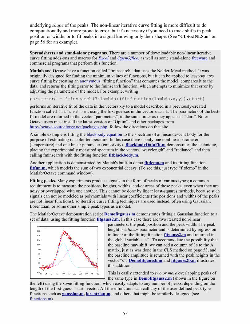
underlying shape of the peaks. The non-linear iterative curve fitting is more difficult to do computationally and more prone to error, but it's necessary if you need to track shifts in peak position or widths or to fit peaks in a signal knowing only their shape. (See “CLSvsINLS.m” on page 56 for an example).

Spreadsheets and stand-alone programs. There are a number of downloadable non-linear iterative curve fitting adds-ons and macros for Excel and OpenOffice, as well as some stand-alone freeware and commercial programs that perform this function.

Matlab and Octave have a function called “fminsearch” that uses the Nelder-Mead method. It was originally designed for finding the minimum values of functions, but it can be applied to least-squares curve fitting by creating an anonymous “fitting function” that computes the model, compares it to the data, and returns the fitting error to the fminsearch function, which attempts to minimize that error by adjusting the parameters of the model. For example, writing

parameters = fminsearch(@(lambda)(fitfunction(lambda,x,y)),start)

performs an iterative fit of the data in the vectors x,y to a model described in a previously-created function called fitfunction, using the first guesses in the vector start. The parameters of the best-fit model are returned in the vector “parameters”, in the same order as they appear in “start”. Note: Octave users must install the latest version of “Optim” and other packages from http:// octave .sourceforge.net/packages.php; follow the directions on that site.

A simple example is fitting the blackbody equation to the spectrum of an incandescent body for the purpose of estimating its color temperature. In this case there is only one nonlinear parameter (temperature) and one linear parameter (emissivity). BlackbodyDataFit.m demonstrates the technique, placing the experimentally measured spectrum in the vectors “wavelength” and “radiance” and then calling fminsearch with the fitting function fitblackbody.m.

Another application is demonstrated by Matlab's built-in demo fitdemo.m and its fitting function fitfun.m , which models the sum of two exponential decays. (To see this, just type “fitdemo” in the Matlab/Octave command window).

Fitting peaks. Many experiments produce signals in the form of peaks of various types; a common requirement is to measure the positions, heights, widths, and/or areas of those peaks, even when they are noisy or overlapped with one another. This cannot be done by linear least-squares methods, because such signals can not be modeled as polynomials with linear coefficients (the positions and widths of the peaks are not linear functions), so iterative curve fitting techniques are used instead, often using Gaussian, Lorentzian, or some other simple peak types as a model.

The Matlab/Octave demonstration script Demofitgauss.m demonstrates fitting a Gaussian function to a set of data, using the fitting function fitgauss2.m. In this case there are two iterated non-linear

parameters: the peak position and the peak width. The peak height is a linear parameter and is determined by regression in line 9 of the fitting function fitgauss2.m and returned in the global variable “c”. To accommodate the possibility that the baseline may shift, we can add a column of 1s to the A matrix, just as was done in the CLS method on page 53, and the baseline amplitude is returned with the peak heights in the vector “c”; Demofitgaussb.m and fitgauss2b.m illustrates this addition.

This is easily extended to two or more overlapping peaks of the same type in Demofitgauss2.m (shown in the figure on

the left) using the same fitting function, which easily adapts to any number of peaks, depending on the length of the first-guess “start” vector. All these functions can call any of the user-defined peak type functions such as gaussian .m, lorentzian .m, and others that might be similarly designed (see functions.m).

55

Variable shapes, such as the Voigt profile, Pearson, and the exponentially-broadened types, are defined not only by a peak position, height, and width, but also by an additional parameter that fine tunes the shape of the peak. If that parameter is equal for all peaks in a group, it can be passed as an additional input argument to the peak function, as shown in VoigtFixedAlpha.m. If the shape parameter is allowed to be different for each peak in the group and is to be determined by iteration (just as is position and width), then the routine must be modified to accommodate three, rather than two, iterated variables, as shown in VoigtVariableAlpha.m. Although the fitting error is lower with variable alphas, the execution time is longer and the alphas values so determined are not very stable, especially for multiple peaks.

Signals with peaks of different shape types in one signal can be fit by the fitting function fitmultiple.m, which takes as input arguments a vector of peak types and a vector of shape variables (To see how this is used, see Demofitmultiple.m).

For the quantitative measurement of peaks, it's instructive to compare the iterative least-squares method with simpler, less computationally-intensive, methods. For example, the measurement of the peak height of a single peak of uncertain width and position could be done simply by taking the maximum of the signal in that region. If the signal is noisy, a more accurate peak height will be obtained if the signal is smoothed beforehand. But smoothing can distort the signal and reduce peak heights. Using an iterative peak fitting method, assuming only that the peak shape is known, can give the best possible accuracy and precision, without requiring smoothing even under high noise conditions, e.g. when the signal-to-noise ratio is 1, as in the demo script SmoothVsFit.m:

True peak height = 1 NumTrials = 100 SmoothWidth = 50 Method Maximum y Max Smoothed y PeakfitAverage peak height 3.65 0.96625 1.0165Standard deviation 0.36395 0.10364 0.11571

If peak area is measured rather than peak height, smoothing is unnecessary (unless to locate the peak beginning and end) but peak fitting still yields the best precision. See SmoothVsFitArea.m.

The Matlab/Octave scipt “CLSvsINLS.m” compares the classical least-squares (CLS) method with three different variations of the iterative method (INLS) method for measuring the peak heights of three Gaussian peaks in a noisy test signal, demonstrating that the fewer the number of unknown parameters, the faster and more accurate is the peak height calculation.

Method Positions Widths Execution time Accuracy CLS known known 0.00133 0.30831 INLS unknown unknown 0.61289 0.6693 INLS known unknown 0.16385 0.67824 INLS unknown known 0.24631 0.33026 INLS unknown known (equal) 0.15883 0.31131

The uncertainty of the peak parameters determined by iterative least-squares fitting is readily determined by the bootstrap sampling method (p. 40-41), as long as the data are unsmoothed. A demonstration of this method is given by the Matlab/Octave function “BootstrapIterativeFit.m”, which creates a single x,y data set consisting of a single noisy gaussian peak, extracts bootstrap samples from that data set, performs an iterative fit to the peak on each of the bootstrap samples, and plots the histograms of peak height, position, and width of the bootstrap samples. The syntax is BootstrapIterativeFit (TrueHeight,TruePosition,TrueWidth, NumPoints,Noise,NumTrials) where TrueHeight is the true peak height of the Gaussian peak, TruePosition is the true x-axis value at the peak maximum, TrueWidth is the true half-width (FWHM) of the peak, NumPoints is the number of points taken for the least-squares fit, Noise is the standard deviation of (normally-distributed) random noise, and NumTrials is the number of bootstrap samples. An typical example for BootstrapIterativeFit (100,100,100,20,10,100); is

56

displayed on the right.

Peak Height Peak Position Peak Width mean: 93.543 97.0227 99.8805 STD: 4.7441 3.8025 5.6621

If you were to run this simulation again, you'd get different results, but the mean peak parameters will always be within two standard deviations of the true values. “BootstrapIterativeFit2.m” is a similar demonstration function for two overlapping Gaussian peaks.

You can create your own fitting functions for any purpose; they are not limited to single algebraic expressions, but can be any complex multistep algorithm. (For example, in the Tfit method in absorption spectroscopy, page 103, a model of the instrumentally-broadened transmission spectrum is fit to the observed transmission data, using a fitting function that performs Fourier convolution of the transmission spectrum with the slit function of the spectrometer, resulting in an extension of the dynamic range and calibration linearity beyond the normal limits). The bootstrap sampling method can be used to predict the precision of the measured model parameters in complicated methods such as this where the algebraic method is impossible. Note: You can download any of the m-files mentioned here from http://tinyurl.com/cey8rwh.

Peak Fitter functions for Matlab and OctaveThese are Matlab or Octave peak fitting programs for time-series signals, which uses an unconstrained non-linear optimization algorithm to decompose a complex, overlapping-peak signal into its component parts. The objective is to determine whether your signal can be represented as the sum of fundamental underlying peaks shapes. They accept signals of any length, including those with non-integer and non-uniform x-values, and can fits groups of peaks with many different peak shape models. There are two different versions, peakfit.m, a command line version for Matlab and Octave (page 90), and ipf.m, a

keypress operated interactive version for Matlab only (page 95). The latest versions of these functions can optionally estimate the expected standard deviation and interquartile range of the peak parameters using the bootstrap sampling method (Page 41 – 42).

Accuracy and precision of peak parameter measurementThis section describes the major sources of error in measuring the peak parameters (peak positions, heights, widths, and areas) by iterative curve fitting.

a. Model errors. Peak shape. If you have the wrong model for your peaks, the results can't be expected to be accurate; for instance, if your actual peaks are Lorentzian in shape, but you fit them with a Gaussian model, or vice versa. For example, a single isolated Gaussian peak at x=5, with a height of 1.000 fits a Gaussian model virtually perfectly, using the Matlab/Octave user-defined peakfit.m function, as shown on the right. The 5th input argument for the peakfit function specifies the shape of peaks to be used in the fit; “1” means Gaussian. (In the following examples, the text after >> is what you type or paste into the command line in Matlab or Octave).>> x=[0:.1:10];y=exp(-(x-5).^2);>> [FitResults,FitError]=peakfit([x' y'],5,10,1,1)

Peak # Position Height Width Area

57

FitResults =1 5 1 .6649 1.7724FitError = 0.001679

The “FitResults” are, from left to right, peak number, peak position, peak height, peak width, and peak area. The fitting error “FitError” is the root mean square difference between the data and the best-fit model, as a percentage of the maximum signal in the fitted region. Note the good agreement of the area measurement (1.7724 with the theoretical area under the curve of exp(-x2), which is the square root of p, or 1.7725.

But this same peak, when fit with a Logistic model (peak shape number 3), gives a fitting error of 1.4% and height and width errors of 3% and 6%, respectively: When fit with a Lorentzian model (peak shape 2), this peak gives a 6% fitting error and height and width errors of 8% and 20%, respectively. So clearly the larger the fitting errors, the larger are the parameter errors, but the parameter errors are of course not equal to the fitting error (that would just be too easy). Also, clearly the peak width and area are the parameters most susceptible to errors. The peak positions, as you can see here, are measured accurately (and will be, even if the model is way wrong, as long as the peak is symmetrical and not highly overlapping with other peaks).

If you do not know the shape of your peaks, you can use use peakfit.m or ipf.m to try different shapes to see if one of the standard shapes included in those programs fits the data; try to find a peak in your data that is typical, isolated, and that has a good signal-to-noise ratio. For example, the Matlab function ShapeTest.m (download from http://tinyurl.com/cey8rwh) creates a test signal consisting of a single peak, adds random white noise, fits it with six different candidate model peak shapes using peakfit.m, plots each fit in a separate figure window, and prints out a table of fitting errors in the command window. In this particular case, the last two shapes fit almost equally well.

Number of peaks. Another source of model error occurs if you have the wrong number of peaks in your model, for example if the signal actually has two peaks but you try to fit it with only one peak. In the example below, a bit of Matlab/Octave code generates a simulated signal with of two Gaussian peaks at x=4 and x=6 with peaks heights of 1.000 and 0.5000 respectively and widths of 1.665, plus random noise with a standard deviation 5% of the height of the largest peak (a signal-to-noise ratio of 20): >> x=[0:.1:10];>> y=exp(-(x-6).^2)+.5*exp(-(x-4).^2) +.05*randn(size(x));

In a real experiment you would not usually know the peak positions, heights, and widths; you would be using curve fitting to measure those parameters. Let's assume that, on the basis of previous experience or some preliminary trial fits, you have established that the optimum peak shape model is Gaussian, but you don't know for sure how many peaks are in this group. If you fit this signal with a single-peak Gaussian model, you get:

>> [FitResults,FitError]=peakfit([x' y'],5,10,1,1)

Peak # Position Height Width Area FitResults = 1 5.5291 0.86396 2.9789 2.7392FitError = 10.467

The residual plot shows a “wavy” structure that's visible in the random scatter of points due to

58

the random noise in the signal. This means that the fitting error is not limited by the random noise; it is a clue that the model is not quite right.

But a fit with two peaks yields much better results (The 4th input argument for the peakfit function specifies the number of peaks to be used in the fit).

>> [FitResults,FitError]=peakfit([x' y'],5,10,2,1)

FitResults =Peak # Position Height Width Area 1 4.0165 0.50484 1.6982 0.91267 2 5.9932 1.0018 1.6652 1.7759FitError = 4.4635

Now the residuals have a random scatter of points, as would be expected if the signal is accurately fit except for the random noise. Moreover, the fitting error is much lower (less than half) of the error with only one peak. In fact, the fitting error is just about what we would expect in this case based on the 5% random noise in the signal (estimating the relative standard deviation of the points in the baseline visible at the edges of the signal).

Because this is a simulation, in which we know beforehand the true values of the peak parameters (peaks at x=4 and x=6 with peaks heights of 1.0 and 0.50 respectively and widths of 1.665), we can actually calculate the parameter errors (the difference between the real peak positions, heights, and widths and the measured values). We see that they are quite accurate (in this case within about 1% relative on the peak height and 2% on the widths), which is actually better than the 5% random noise in this signal because of the averaging effect of fitting to multiple data points in the signal.

In real experimental work, of course, you usually don't know the right answers beforehand, so that's why it's important to use methods that work well when you do know.

But if going from one peak to two peaks gave us a better fit, why not go to three peaks? Changing the number of peaks to three (second-to-last argument) gives these results:

>> [FitResults,FitError]=peakfit([x' y'],5,10,3,1)

Peak # Position Height Width AreaFitResults = 1 4.0748 0.51617 1.7874 0.98212 2 6.7799 0.089595 2.0455 0.19507 3 5.9711 0.94455 1.53 1.5384FitError = 4.3878

The fitting algorithm has now tried to fit an additional low-amplitude peak (numbered peak 2 in this case) located at x=6.78. The fitting error is actually lower than for the 2-peak fit, but only slightly lower, and the residuals are no less visually random that with a 2-peak fit. So, knowing nothing else, a 3-peak fit might be rejected on that basis alone. In fact, there is a serious downside to fitting more peaks than are present in the signal: it increases the parameter measurement errors of the peaks that are

59

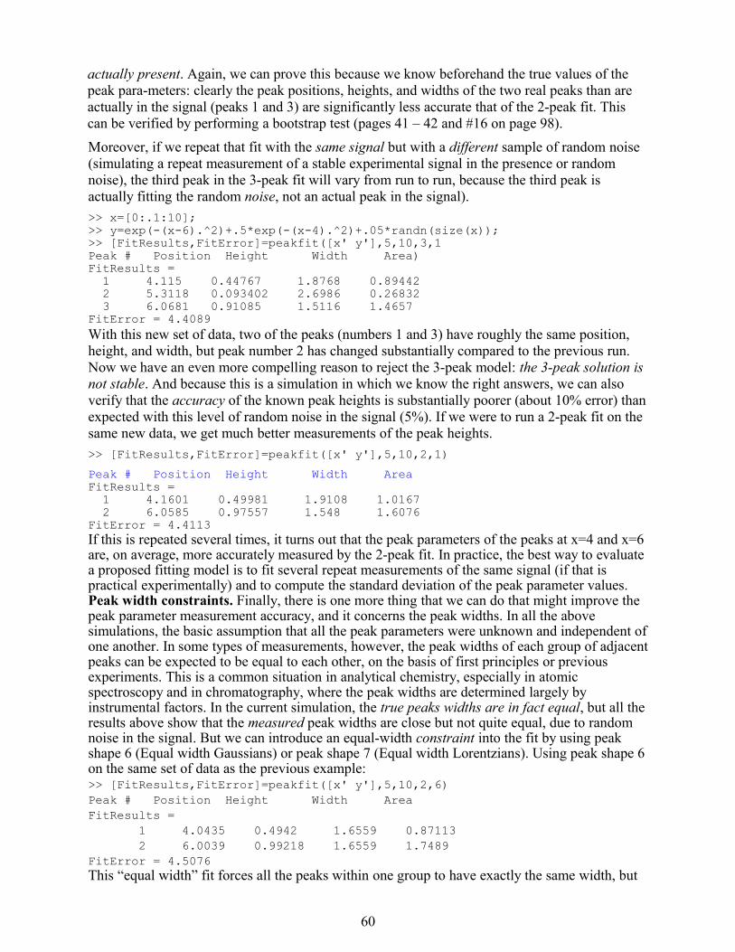
actually present. Again, we can prove this because we know beforehand the true values of the peak para-meters: clearly the peak positions, heights, and widths of the two real peaks than are actually in the signal (peaks 1 and 3) are significantly less accurate that of the 2-peak fit. This can be verified by performing a bootstrap test (pages 41 – 42 and #16 on page 98).

Moreover, if we repeat that fit with the same signal but with a different sample of random noise (simulating a repeat measurement of a stable experimental signal in the presence or random noise), the third peak in the 3-peak fit will vary from run to run, because the third peak is actually fitting the random noise, not an actual peak in the signal).

>> x=[0:.1:10];>> y=exp(-(x-6).^2)+.5*exp(-(x-4).^2)+.05*randn(size(x));>> [FitResults,FitError]=peakfit([x' y'],5,10,3,1Peak # Position Height Width Area)FitResults = 1 4.115 0.44767 1.8768 0.89442 2 5.3118 0.093402 2.6986 0.26832 3 6.0681 0.91085 1.5116 1.4657FitError = 4.4089With this new set of data, two of the peaks (numbers 1 and 3) have roughly the same position, height, and width, but peak number 2 has changed substantially compared to the previous run. Now we have an even more compelling reason to reject the 3-peak model: the 3-peak solution is not stable. And because this is a simulation in which we know the right answers, we can also verify that the accuracy of the known peak heights is substantially poorer (about 10% error) than expected with this level of random noise in the signal (5%). If we were to run a 2-peak fit on the same new data, we get much better measurements of the peak heights.

>> [FitResults,FitError]=peakfit([x' y'],5,10,2,1)

Peak # Position Height Width AreaFitResults = 1 4.1601 0.49981 1.9108 1.0167 2 6.0585 0.97557 1.548 1.6076FitError = 4.4113If this is repeated several times, it turns out that the peak parameters of the peaks at x=4 and x=6 are, on average, more accurately measured by the 2-peak fit. In practice, the best way to evaluate a proposed fitting model is to fit several repeat measurements of the same signal (if that is practical experimentally) and to compute the standard deviation of the peak parameter values. Peak width constraints. Finally, there is one more thing that we can do that might improve the peak parameter measurement accuracy, and it concerns the peak widths. In all the above simulations, the basic assumption that all the peak parameters were unknown and independent of one another. In some types of measurements, however, the peak widths of each group of adjacent peaks can be expected to be equal to each other, on the basis of first principles or previous experiments. This is a common situation in analytical chemistry, especially in atomic spectroscopy and in chromatography, where the peak widths are determined largely by instrumental factors. In the current simulation, the true peaks widths are in fact equal, but all the results above show that the measured peak widths are close but not quite equal, due to random noise in the signal. But we can introduce an equal-width constraint into the fit by using peak shape 6 (Equal width Gaussians) or peak shape 7 (Equal width Lorentzians). Using peak shape 6 on the same set of data as the previous example:>> [FitResults,FitError]=peakfit([x' y'],5,10,2,6)Peak # Position Height Width AreaFitResults = 1 4.0435 0.4942 1.6559 0.87113 2 6.0039 0.99218 1.6559 1.7489FitError = 4.5076This “equal width” fit forces all the peaks within one group to have exactly the same width, but

60

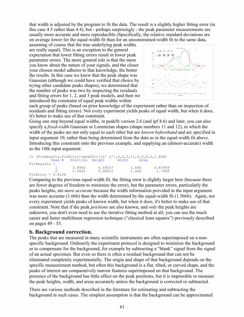
that width is adjusted by the program to fit the data. The result is a slightly higher fitting error (in this case 4.5 rather than 4.4), but - perhaps surprisingly - the peak parameter measurements are usually more accurate and more reproducible (Specifically, the relative standard deviations are on average lower for the equal-width fit than for an unconstrained-width fit to the same data, assuming of course that the true underlying peak widths are really equal). This is an exception to the general expectation that lower fitting errors result in lower peak parameter errors. The more general rule is that the more you know about the nature of your signals, and the closer your chosen model adheres to that knowledge, the better the results. In this case we knew that the peak shape was Gaussian (although we could have verified that choice by trying other candidate peaks shapes), we determined that the number of peaks was two by inspecting the residuals and fitting errors for 1, 2, and 3 peak models, and then we introduced the constraint of equal peak widths within each group of peaks (based on prior knowledge of the experiment rather than on inspection of residuals and fitting errors). Not every experiment yields peaks of equal width, but when it does, it's better to make use of that constraint.

Going one step beyond equal widths, in peakfit version 2.6 (and ipf 8.6) and later, you can also specify a fixed-width Gaussian or Lorentzian shapes (shape numbers 11 and 12), in which the width of the peaks are not only equal to each other but are known beforehand and are specified in input argument 10, rather than being determined from the data as in the equal-width fit above. Introducing this constraint onto the previous example, and supplying an (almost-accurate) width as the 10th input argument:

>> [FitResults,FitError]=peakfit([x' y'],0,0,2,11,0,0,0,0,1.666) Peak # Position Height Width Area FitResults = 1 3.9943 0.49537 1.666 0.87849 2 5.9924 0.98612 1.666 1.7488FitError = 4.8128

Comparing to the previous equal-width fit, the fitting error is slightly larger here (because there are fewer degrees of freedom to minimize the error), but the parameter errors, particularly the peaks heights, are more accurate because the width information provided in the input argument was more accurate (1.666) than the width determined by the equal-width fit (1.5666). Again, not every experiment yields peaks of known width, but when it does, it's better to make use of that constraint. Note that if the peak positions are also known, and only the peak heights are unknown, you don't even need to use the iterative fitting method at all; you can use the much easier and faster multilinear regression technique (“classical least squares”) previously described on pages 49 - 53.

b. Background correction. The peaks that are measured in many scientific instruments are often superimposed on a non-specific background. Ordinarily the experiment protocol is designed to minimize the background or to compensate for the background, for example by subtracting a “blank” signal from the signal of an actual specimen. But even so there is often a residual background that can not be eliminated completely experimentally. The origin and shape of that background depends on the specific measurement method, but often this background is a flat, tilted, or curved shape, and the peaks of interest are comparatively narrow features superimposed on that background. The presence of the background has little effect on the peak positions, but it is impossible to measure the peak heights, width, and areas accurately unless the background is corrected or subtracted.

There are various methods described in the literature for estimating and subtracting the background in such cases. The simplest assumption is that the background can be approximated

61

as a simple function in the local region of group of peaks being fit together, for example as a constant (flat), straight line (linear), or curved line (quadratic). This is the basis of the "autozero" modes in the ipf.m, iSignal.m, and iPeak.m functions, which are selected by the T key to cycle thorough none, linear, quadratic, and flat modes. In the flat mode, a constant baseline is included in the curve fitting calculation, as described on page 55. In linear mode, a straight-line baseline connecting the two ends of the signal segment in the upper panel will be automatically subtracted. In quadratic mode, a parabolic baseline is subtracted. (In the last two modes, you must adjust the pan and zoom controls to isolate the group of overlapping peaks to be fit, so that the signal returns to the local background at the left and right ends of the window).

Example of an experimental chromatographic signal. From left to right, (1) Raw data with peaks superimposed on a sloping baseline. One group of peaks is selected using the pan and zoom controls, adjusted so that the signal returns to the local background at the edges of the segment displayed in the upper window; (2) The linear baseline is subtracted when the “autozero” mode 1 in ipf.m; (3) the signal in this region is fit with a three-peak Gaussian model, activated by pressing the keys: 3, G, F (3 peaks, Gaussian, Fit).

Left: Raw data with peaks superimposed on baseline. Right: Background subtracted from the entire signal using the multi-point background subtraction function in iPeak .m (ipf.m and iSignal have the same function).

Alternatively, it's possible to subtract the background from the entire signal first, before further operations are performed. The simplest assumption is that the back-ground is piecewise linear, that is, can be approximated as a series of small straight line segments. This is the basis of the multi-point background subtraction mode in ipf.m (page 95), iPeak.m (page 76), and in iSignal.m (page 85). The user enters the number of points that is thought to be sufficient to define the baseline, then clicks where the baseline is thought to be along the entire length of the signal in the lower whole-signal display (e.g. on the valleys between the peaks), and the program interpolates between the clicked points and subtracts the piecewise linear background from the original signal.Sometimes, even without an actual baseline present, the peaks may overlap enough so that the signal never return to the baseline, making it seem that there is a baseline to be corrected. This is not an uncommon situation with peaks shapes that have gradually sloping sides, such as the Lorentzian, as shown in this example. Curve fitting without baseline correction will work in that case. In some cases the background may be caused by a broad peak whose maximum falls outside of the range of data acquired. It may still be possible to fit the off-screen peak simply by

62

including extra peak in the model to account for the baseline. (Don't use the equal-width shapes for this, because it's likely that the background peak is broader than the measured peaks).

c. Random noise in the signal. Any experimental signal has a certain amount of random noise, which means that the individual data points scatter randomly above and below their mean values. The assumption is ordinarily made that the scatter is equally above and below the true signal, so that the long-term average approaches the true mean value; the noise “averages to zero”, as it is often said. The practical problem is that any given recording of the signal contains only one finite sample of the noise. If another recording of the signal is made, it will contain another independent sample of the noise. These noise samples are not infinitely long and therefore do not represent the true long-term nature of the noise. This presents two problems: (1) an individual sample of the noise will not “average to zero” and thus the parameters of the best-fit model will not necessarily equal the true values, and (2) the magnitude of the noise during one sample might not be typical; the noise might have been randomly greater or smaller than average during that time. This means that the mathematical “propagation of error” methods, which seek to estimate the likely error in the model parameters based on the noise in the signal, will underestimate the error if the noise in that sample happens to be lower than average and overestimate the error if the noise happens to be larger than average in that sample.

A better way to estimate the parameter errors is to record multiple samples of the signal, fit each of those separately, compute the models parameters from each fit, and calculate the standard error of each parameter. This is exactly what the script Demo Peakfit .m does (which requires the peakfit .m function) for simulated noisy peak signals such as those illustrated in the figure below. It's easy to demonstrate that, as expected, the average fitting error precision and the relative standard deviation of the parameters increases directly with the random noise level in the signal. But the precision and the accuracy of the measured parameters also depend on which parameter it is (peak positions are always measured more accurately than their heights, widths, or areas) and on the peak height and extent of peak overlap (the two left-most peaks in this example are not only weaker but also more overlapped that the right-most peak, and therefore exhibit poorer parameter measurements). In this example, the fitting error is 1.6% and the percent relative standard deviation of the parameters ranges from 0.05% for the peak position of the largest peak to 12% for the peak area of the smallest peak.

The errors in the values of peak parameters measured by curve fitting depend not only on the characteristics of the peaks in question and the signal-to-noise ratio, but also upon other peaks that are overlapping it. From left to right: (1) a single peak at x=100 with a peak height of 1.0 and width of 30 is fit with a Gaussian model, yielding a relative fit error of 4.9% and relative standard deviation of peak position, height, and width of 0.2%, 0.95%, and 1.5% , respectively. (2) The same peak, with the same noise level but with another peak overlapping it, reduces the relative fit error to 2.4% (because the addition if the second peak increases overall signal amplitude), but increases the relative standard deviation of peak position, height, and width to 0.84%, 5%, and 4% - a seemingly better fit, but with poorer precision for the first peak. (3) The addition of a third peak further reduces the fit error to 1.6% , but the relative standard deviation of peak position, height, and width of the first peak are still 0.8%, 5.8%, and 3.64%, about the same as with two peaks, because the third peak does not overlap the first one significantly

63

If it is not possible to record multiple samples of the signal, or if the average noise in the signal is not known, or if its probability distribution is uncertain, it is still possible to use the bootstrap sampling method to estimate the uncertainty of the peak heights, positions, and widths, as described on page 41 - 42, as long as the data are unsmoothed. The latest versions of peakfit.m (page 93, example 15) and of ipf.m (page 95) have a function that estimates the expected standard deviation of the peak parameters from a single signal, using the bootstrap method (#16 on page 98). Don't smooth the data before curve fitting; it will not actually reduce the accuracy of peak parameter measurement and it will cause the bootstrap method to seriously underestimate the parameter errors. The same thing occurs if the noise is “pink” (page 8) ; the errors will be underestimated by the bootstrap.

One way to reduce the effect of noise is to take more data per signal. If the experiment makes it possible to reduce the x-axis interval between points, or to take multiple readings at each x-axis value, then the resulting increase in the number of data points in each peak should help reduce the effect of noise. As a demonstration, using the script Demo Peakfit .m to create a simulated overlapping peak signal like that shown above right, it's possible to change the interval between x values and thus the total number of data points in the signal. With a noise level of 1% and 75 points in the signal, the fitting error is 0.35 and the average parameter error is 0.8%. With 300 points in the signal and the same noise level, the fitting error is essentially the same, but the average parameter error drops to 0.4%, suggesting that the accuracy of the measured parameters varies inversely with the square root of the number of data points in the peaks.

The figure on the right below illustrates the importance of sampling interval and data density. The signal consists of two Gaussian peaks, one located at x=50 and the second at x=150. Both peaks have a peak height of 1.0 and a peak half-width of 10 units, and normally-distributed random white noise with a standard deviation of 0.1 has been added to the entire signal. The x-axis sampling interval, however, is different for the two peaks; it's 0.1 for the first peaks and 1.0 for the second peak. This means that the first peak is characterized by ten times more data points that the second peak. When you fit these peaks to a Gaussian model (e.g. using peakfit.m or ipf.m), you will find that the parameters of the first peak are measured more accurately than the second, even though the fitting error is not much different (because the noise is the same): First peak: Second peak: Percent Fitting Error = 7.6434% Percent Fitting Error = 8.8827% Position Height Width Position Height Width 49.95 1.005 10.11 149.64 1.0313 9.94

Iterative fitting errors. Unlike multiple linear regression curve fitting, iterative methods may not converge on the exact same model parameters each time the fit is repeated with slightly different starting values (first guesses). The Interactive Peak Fitter (ipf.m, page 95) makes it easy to test this, because it uses slightly different starting values each time the signal is fit (by pres-sing the F key in ipf.m, for example). Even better, by pressing the X key, the ipf.m func-tion silently computes 10 fits with different starting values and takes the one with the lowest fitting error. A basic assumption of any curve fitting operation is that the fitting error (the RMS difference between the model and the data) is minimized, the parameter errors (the difference between the actual parameters and the parameters of the best-fit model) will also be minimized. This is usually a good assumption. For example, the graph on the right shows typical percent parameters errors as a function of fitting error for the left-most peak in one sample of the simulated signal generated by the script

64

Demo Peakfit .m (shown in the previous section). The variability of the fitting error here is caused by random small variations in the first guesses, rather than by random noise in the signal. In many practical cases there is enough random noise in the signals that the iterative fitting errors within one sample of the signal are small compared to the random noise errors between samples.

Remember that the variability in measured peak parameters from fit to fit of a single sample of the signal is not a good estimate of the precision or accuracy of those parameters, for the simple reason that those results represent only one sample of the signal, noise, and background. The sample-to-sample variations are likely to be much greater than the within-sample variations due to the iterative curve fitting. (In this case, a “sample” is a single recording of signal). To estimate the contribution of random noise to the variability in measured peak parameters when only a single sample if the signal is available, use the bootstrap method (page 41 – 42).

So, to sum up, we can make the following observations about the accuracy of peak parameters: (1) the errors depend on the appropriateness of the model and number of peaks; (2) the errors increase as the noise in the data and the fitting error increases; (3) the errors are typically least for peak position and worse for peak width and area; (4) the errors depend on the accuracy of the baseline correction, the data density (number of independent data points in the width of each peak), and the extent of peak overlap (the parameters of isolated peaks are easier to measure than highly overlapped peaks); (5) if only a single signal is available, the effect of noise on the standard deviation of the peak parameters can be predicted approximately by the bootstrap method.

65

Fitting signals that are subject to exponential broadening. Data Matrix2 (right) is a computer-generated test signal consisting of 16 symmetrical Gaussian peaks with random white noise added. The peaks occur in groups of 1, 2, or 3 overlapping peaks, and the peak maxima are located at exactly integer values of x from 300 to 3900 (on the 100's) and the peak widths are always exactly 60 units. The peak heights vary from 0.06 to 1.85. The standard deviation of the noise is 0.01. (You can use this signal to test curve-fitting programs and to determine the accuracy of their measurements of peak parameters. Download these mat files from the bottom of http://tinyurl.com/cey8rwh, put it in the Matlab/Octave path, then type “load Data Matrix2” to load it into the workspace). Data Matrix3 (below left) is an exponentially broadened version of DataMatrix2, with a “time constant” of 33 points on the x-axis. The result of the exponential broadening is that all the peaks

in this signal are asymmetrical, their peak maxima are shifted slightly to longer x values, and their peak heights are smaller and their peak widths are larger than the corresponding peaks in DataMatrix2. Also, the random noise is damped in this signal compared to the original and is no longer “white”, as a consequence of the broadening. This type of effect is common in physical measurements and often arises from some physical or

electrical effect in the measurement system that is apart from the fundamental peak characteristics. In such cases it is usually desirable to compensate for the effect of the broadening, either by Fourier deconvolution (page 32) or by curve fitting, in an attempt to measure what the peak parameters would have been before the broadening (and also to measure the broadening itself). This can be done for Gaussian peaks that are exponentially broadened by using the “ExpGaussian” peak shape in peakfit.m and ifp.m. The example illustrated on the right above focuses on the single isolated peak whose “true” peak position, height, width, and area in the original unbroadened signal, are 2800, 0.52, 60, and 33.2 respectively. (The relative standard deviation of the noise is 0.01/0.52=2%.) In the broadened signal, the peak is visibly asymmetrical, the peak maximum is shifted to larger x values, and it has a shorter height and larger width, as demonstrated by the attempt to fit a normal (symmetrical) Gaussian to the broadened peak. (Note that the peak area, in contrast, is not much effected).

>> load DataMatrix3>> (DataMatrix3);

Peak Shape = GaussianAutozero ONNumber of peaks = 1Fitted range = 2640 - 2979.5 (339.5) (2809.75) Percent Error = 1.2084Peak # Position Height Width Area1 2814.832 0.4510 68.4412 32.8594

66

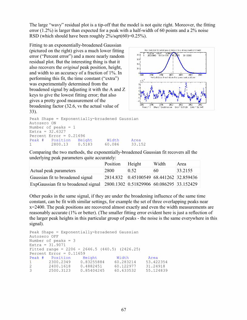
The large “wavy” residual plot is a tip-off that the model is not quite right. Moreover, the fitting error (1.2%) is larger than expected for a peak with a half-width of 60 points and a 2% noise RSD (which should have been roughly 2%/sqrt(60)=0.25%).

Fitting to an exponentially-broadened Gaussian (pictured on the right) gives a much lower fitting error (“Percent error”) and a more nearly random residual plot. But the interesting thing is that it also recovers the original peak position, height, and width to an accuracy of a fraction of 1%. In performing this fit, the time constant (“extra”) was experimentally determined from the broadened signal by adjusting it with the A and Z keys to give the lowest fitting error; that also gives a pretty good measurement of the broadening factor (32.6, vs the actual value of 33).

Peak Shape = Exponentially-broadened GaussianAutozero ONNumber of peaks = 1Extra = 32.6327Percent Error = 0.21696Peak # Position Height Width Area1 2800.13 0.5183 60.086 33.152

Comparing the two methods, the exponentially-broadened Gaussian fit recovers all the underlying peak parameters quite accurately:

Position Height Width Area

Actual peak parameters 2800 0.52 60 33.2155

Gaussian fit to broadened signal 2814.832 0.45100549 68.441262 32.859436

ExpGaussian fit to broadened signal 2800.1302 0.51829906 60.086295 33.152429

Other peaks in the same signal, if they are under the broadening influence of the same time constant, can be fit with similar settings, for example the set of three overlapping peaks near x=2400. The peak positions are recovered almost exactly and even the width measurements are reasonably accurate (1% or better). (The smaller fitting error evident here is just a reflection of the larger peak heights in this particular group of peaks - the noise is the same everywhere in this signal).

Peak Shape = Exponentially-broadened GaussianAutozero OFFNumber of peaks = 3Extra = 31.9071Fitted range = 2206 - 2646.5 (440.5) (2426.25) Percent Error = 0.11659Peak # Position Height Width Area1 2300.2349 0.83255884 60.283214 53.4223542 2400.1618 0.4882451 60.122977 31.249183 2500.3123 0.85404245 60.633532 55.124839

67

The residual plots in both of these examples still have some “wavy” character, rather than being completely random and “white”. The exponential broadening smooths out any white noise in the original signal that was introduced before the exponential effect, acting as a low-pass filter in the time domain and resulting in a low-frequency dominated “pink” noise, which is what remains in the residuals after the broadened peaks have been fit as well as possible. On the other hand, white noise that is introduced after the exponential effect would continue to appear white and random on the residuals. In real experimental data, both types of noise may be present in varying amounts.

One final caveat: peak asymmetry similar to exponential broadening can in principle be the result a pair of closely-spaced peaks of different peak heights. In fact, a single exponential broadened Gaussian peak can be fit with two or three symmetrical Gaussians to a fitting error at least as low as a single exponential broadened Gaussian fit. This makes it hard to distinguish between these two models on the basis of fitting error alone. However, this can usually be decided by inspecting the other peaks in the signal: in many experiments, the same exponential broadening applies to every peak in the signal, and the broadening is either constant or changes gradually over the length of the signal. On the other hand, it is less likely that every peak in the signal will be accompanied by a smaller side peak that varies in exactly this way. So, if a only one or a few peaks exhibit asymmetry, and the others are symmetrical, it's most likely that the asymmetry is due to closely-spaced peaks of different peak heights. If all peaks have the same or similar asymmetry, it's more likely to be caused by a broadening factor that applies to the entire signal. Human judgment, based on knowledge of the experimental system and the types of signals it generates, is always valuable and is often essential.

More generally, it is technically possible to fit any arbitrary peak, symmetrical or not, with the sum of a number of Gaussians; and the greater the number of Gaussians, the lower will be the fitting error. But the Gaussian peak parameters so determined will usually not be reproducible with respect to small changes in starting values or to variations in the noise in the data.

68

Effect of smoothing: to smooth or not to smooth In general, it is not advisable to smooth a signal before applying least-squares fitting (reference 43), because doing so might distort the signal, make it hard to evaluate the residuals properly, and bias the results of bootstrap sampling estimations of precision, causing it to underestimate the between-signal variations in peak parameters.

The Matlab/Octave script SmoothOptimization.m (download from http://tinyurl.com/cey8rwh) compares the effect of smoothing on the measurements of peak height of a Gaussian peak with a half-width of 166 points, plus white noise with a signal-to-noise ratio (SNR) of 10, using three different methods:

(a) simply taking the single point at the center of the peak as the peak height; (b) using the gaussfit method to fit the top half of the peak (page 43), and (c) fitting the entire signal with a Gaussian using the iterative method (page 54).

The results of 150 trials with independent white noise samples are shown on the left: a typical raw signal is shown in the upper left. The other three plots show the effect of the SNR of the measured peak height vs the smooth ratio (the ratio of the smooth width to the half-width of the peak) for those three measurement methods.

The results show that the simple single-point measurement is indeed much improved by smoothing, as would be expected; however, the optimum SNR is achieved only when the smooth ratio approaches 1.0 (which improves the SNR by roughly the square root of the peak width of 166 points), but that much smoothing distorts the peak shape

significantly, reducing the peak height by about 40%. The curve-fitting methods are much less effected by smoothing and the iterative method hardly at all. In terms of harmonic analysis (page 26), smoothing removes only the high-frequency noise, leaving the low-frequency noise where most of the signal information is concentrated, resulting in no real improvement. Smoothing just makes things look better.

So the conclusion is that you should not smooth prior to curve-fitting, because it will distort the peak and will not gain any significant SNR advantage. The only situation where it might be advantageous so smooth is when the noise in the signal is high-frequency weighted (page 7) or if the signal is contaminated with high-amplitude narrow spike artifacts, in which case a median-based pre-filter is useful (page 14).

69

Software details1. SPECTRUM for Macintosh OS 7 or 8Some of the figures in this essay are screen images from S.P.E.C.T.R.U.M. (Signal Processing for Experimental Chemistry Teaching and Research/ University of Maryland), a simple Macintosh program that I developed in 1989 for teaching signal processing to chemistry students. Unfortunately it runs only in Mac OS 8.1 and earlier.

SPECTRUM is designed for post-run (rather than real-time) processing of “spectral” or time- series data (y values at equally-spaced x intervals), such as spectra, chromatograms, electrochemical signals, etc. The program enhances the information content of instrument signals, for example by reducing noise, improving resolution, compensating for instrumental artifacts, and testing hypotheses.

SPECTRUM was the winner of two EDUCOM/NCRIPTAL national software awards in 1990, for Best Chemistry software and for Best Design.

Features

• Reads one- or two- column (y-only or x-y) text data tables with either tab or space separators

• Displays fast, labeled plots in standard re-sizable windows with full x- and y-axis scale expansion and a mouse-controlled measurement cursor

• Addition, subtraction, multiplication, and division of two signals• Two kinds of smoothing. • Three kinds of differentiation• Integration• Resolution enhancement• Interpolation • Fused peak area measurement by perpendicular drop or tangent skim methods, with

mouse-controlled setting of start and end points• Fourier transformation • Power spectra

70

• Fourier filtering • Convolution and deconvolution • Cross- and auto-correlation • Built-in signal simulator with Gaussian and Lorentzian bands, sine wave and normally-

distributed random noise• A number of other useful functions, including: inspect and edit individual data points,

normalize, histogram, interpolate, zero fill, group points by 2s, bridge segment, superimpose, extract subset of points, concatenate, reverse X-axis, rotate, set X axis values, reciprocal, log, ln, antilog, antiln, standard deviation, absolute value, square root

SPECTRUM can be used both as a research tool and as an instructional aid in teaching signal processing techniques. The program and its associated tutorial was originally developed for students of analytical chemistry, but the program could be used in any field in which instrumental measurements are used: e.g. chemistry, biochemistry, physics, engineering, medical research, clinical psychology, biology, environmental and earth sciences, agricultural sciences, or materials testing.

SPRECTUM performs only polynomial curve fitting and does not include non-linear iterative curve fitting.

Machine Requirements: SPECTRUM runs only on older Macintosh models running OS 7 or 8, minimum 1 MByte RAM, any standard printer. Color screen desirable. SPECTRUM has been tested on most Macintosh models and on all versions of the operating system through OS 8.1. No PC version or more recent Mac version is available or planned, but if you have some older model Macs laying around, you might find this program useful. SPECTRUM was written in Borland's Turbo Pascal in 1989; that firm had long been out of business, neither Turbo Pascal nor the executable code generated by that compiler runs on current Macs, and therefore there is no way for me to update SPECTRUM without completely re-writing it in another language.

The full version of SPECTRUM 1.1 is now available as freeware, and can be downloaded from http://terpconnect.umd.edu/~toh/spectrum/. There are two versions:

SPECTRUM 1.1e: Signals are stored internally as extended-precision real variables and there is a limit of 1024 points per signal. This version performs all its calculations in extended precision and thus has the best dynamic range and the smallest numeric round-off errors. The download address of this version in HQX format is http://terpconnect.umd.edu/~toh/spectrum/SPECTRUM11e.hqx.

SPECTRUM 1.1b: Signals are stored internally as single-precision real variables and there is a limit of 4000 points per signal. This version is less precise in its calculations (has more numerical round-off error) than the other version, but allows signals with data more points. The download address of this version in HQX format is http://terpconnect.umd.edu/~toh/spectrum/SPECTRUM11b.hqx.

The two versions are otherwise identical.

There is also a documentation package (located at http://terpconnect.umd.edu/~toh/spectrum/SPECTRUMdemo.hqx) consisting of:

a. Reference manual. Macwrite format (Can be opened from within MacWrite, Microsoft Word, ClarisWorks, WriteNow, and most other full-featured Macintosh word processors). Explains each menu selection and describes the algorithms and mathematical formulae for each operation. The SPECTRUM Reference Manual is also available separately in PDF format at http://terpconnect.umd.edu/~toh/spectrum/SPECTRUMReferenceManual.pdf.

71

b. Signal processing tutorial. Macwrite format (Can be opened from within MacWrite, Microsoft Word, ClarisWorks, WriteNow, and most other full-featured Macintosh word processors). Self-guided tutorial on the applications of signal processing in analytical chemistry. This tutorial is also available on the Web at (http://terpconnect.umd.edu/~toh/Chem498C/SignalProces sing.html)

c. Tutorial signals: A library of prerecorded data files for use with the signal processing tutorial. These are plain decimal ASCII (tab-delimited) data files.

These files are binhex encoded: use Stuffit Expander to decode and decompress as usual. If you are downloading on a Macintosh, all this should happen completely automatically. If you are viewing this on-line, shift-click on the download links above to begin the download. If you are using the ARDI Executor Mac simulator, download the “HQX” files to your C drive, launch Executor, then open the downloaded HQX files with Stuffit Expander, which is pre-loaded into the Executor Macintosh environment. Stuffit Expander will automatically decode and decompress the downloaded files.

Note: Because it was developed for academic teaching application where the most modern and powerful models of computers may not be available, SPECTRUM was designed to be “lean and mean” - that is, it has a simple Macintosh-type user interface and very small memory and disk space requirements. It will work quite well on Macintosh models as old as the Macintosh II, and will even run on older monochrome models (with some cramping of screen space). It does not require a math co-processor.

(c) 1989 T. C. O'Haver. This program is free and may be freely distributed. It may be included on CD-ROM collections or other archives.

72

2. Matlab and OctaveMatlab is a high-performance commercial numerical computing environment and programming language that is very widely used in research and education. See http://en.wikipedia.org/wiki/ MATLAB for a general description. There are several good on-line tutorials, YouTube videos, and collections of sample code:

a. Video Tutorials for New MATLAB Users (http://www.youtube.com/results?search_query= matlab +tutorial&aq=f ).

b. A Brief Introductory Guide to MATLAB. (http://www.cs.unc.edu/~snoeyink/c/c205/matlab.htm)

c. Matlab Summary and Tutorial. (http://www.math.ufl.edu/help/ matlab -tutorial/)

d. A Practical Introduction to Matlab (http://www.math.mtu.edu/~msgocken/intro/intro.html)

e. Matlab Chemometrics Index http://www.mathworks.com/ matlab central/linkexchange/?term=chemometrics

f. Introduction to Matlab: http://homepages.math.uic.edu/~jan/mcs320s07/

g. Practical Statistical Signal Processing using MATLAB: http://www.aticourses.com/sampler/Practical%20Signal%20Processing%20using %20 MATLAB .pdf.

i. Multivariate Curve Resolution. http://www.mcrals.info/

h. MATLAB Tutorials and Learning Resources: http://www.mathworks.com/academia/student_center/tutorials/launchpad.html

A Google or YouTube search for “signal processing” or “matlab” will often prove useful in turning up recently available tutorial materials. Several experienced Matlab users, as well as the MathWorks company itself, have produced many tutorial YouTube videos.

A collection of downloadable Matlab modules that I have written is available on http://terpconnect.umd.edu/~toh/spectrum/SignalProcessingTools.html. These are described in the following sections of this document.

Octave. There are free alternatives to the relatively expensive Matlab that operate in much the same way. I recommend Octave (http://www.gnu.org/software/ octave /); it's free and almost completely compatible with Matlab; in fact, all of my command-line functions, scripts, demos, and examples will work in the latest version of Octave without change. (The keyboard-operated interactive functions of iPeak, iSignal, iFilter, and ipf do not currently work in Octave). There are Windows, Mac, and Unix versions; you can download Windows versions from Octave Forge (http://sourceforge.net/projects/ octave /). Be sure to install all the “packages”. Installation of Octave is somewhat more laborious than installing a commercial package like Matlab, and Octave is slower that Matlab computationally (see http://terpconnect.umd.edu/~toh/spectrum/TimeTrial.txt for specific execution time comparisons for typical signal processing tasks). There is lots of help online: Google “GNU Octave” or see the YouTube videos for help.

SciLab (http://www.scilab.org/ ) and FreeMat (http://freemat.sourceforge.net/) are other programs similar to Matlab. For a discussion of other possibilities, see http://www.dspguru.com/dsp/links/ matlab -clones.

73

3. Peak Finding and MeasurementA common requirement in signal processing is to detect peaks in a signal and to measure their positions, heights, and widths. A common way to do this is to make use of the fact that the first derivative (page 17) of a peak has a downward-going zero-crossing at the peak maximum. But the presence of random noise in real experimental signal will cause many false zero-crossing simply due to the noise. To avoid this problem, the technique described here first smooths (page 11) the first derivative of the signal, before looking for downward-going zero-crossings, and then it takes only those zero crossings whose slope exceeds a certain predetermined minimum called the “slope threshold”) at a point where the original signal exceeds a certain minimum (called the “amplitude threshold”). By optimizing the smooth width, slope threshold, and amplitude threshold, it's possible to detect only the desired peaks and ignore peaks that are too small, too wide, or too narrow. Moreover, because smoothing can distort peak signals, reducing peak heights and increasing peak widths (page 11), this technique estimates the position, height, and width of each peak by least-squares curve-fitting (page 37) of a segment of the original unsmoothed signal in the vicinity of the zero-crossing. As a result, even if heavy smoothing of the first derivative is necessary to provide reliable discrimination against noise peaks, the peak parameters extracted by curve fitting are not distorted. (This is useful primarily for signals that have several data points in each peak, not for spikes that have only one or two points). The technique is capable of measuring peak positions and heights quite accurately, but the measurements of peak widths and areas is accurate only if the peaks are approximately Gaussian (or Lorentzian, using findpeaksL.m) in shape. (For the most accurate measurement of highly overlapped peaks of any shape, iPeak version 3 or 4 is capable of utilizing non-linear iterative curve fitting. See Page 54). The routine is available in two different versions: (1) a command-line function, avail-able in several different variations; (2) an interactive keypress-operated function ( ipeak .m) for adjusting the peak detection criteria in real-time to optimize for any particular peak type. If you are viewing this on-line, click here to download the ZIP file “Peakfinder.zip” that includes supporting functions, several self-contained demos to show how it works, and two interactive versions. Download from http://tinyurl.com/cey8rwh.

The findpeaks and findvalleys functions (findpeaks .m and findvalleys.m)P=findpeaks(x,y,SlopeThreshold,AmpThreshold,SmoothWidth,FitWidth, smoothtype)

This is the basic function for Matlab or Octave to locate and measure the positive peaks in a noisy data sets. It is an alternative to the findpeaks function in the Signal Processing Toolkit. It detects peaks by looking for downward zero-crossings in the smoothed first derivative that exceed SlopeThreshold and peak amplitudes that exceed AmpThreshold, and determines the position, height, and approximate width of each peak by least-squares curve-fitting the top part of the peak. The function returns a peak table matrix P containing the peak number and the estimated position, height, width, and area of each peak. The signal is passed to the function in the vectors x and y (x = independent variable, y = dependent variable). The other parameters are user-adjustable:SlopeThreshold - Slope of the smoothed first-derivative that is taken to indicate a peak. This discriminates on the basis of peak width. Larger values of this parameter will neglect broad features of the signal. A reasonable value for Gaussian peaks is 0.7*WidthPoints^-2, where WidthPoints is the number of data points in the half-width of the peak.AmpThreshold - Discriminates on the basis of peak height. Any peaks with height less than this value are ignored.SmoothWidth - Width of the smooth function that is applied to data before the slope is measured. Larger values of SmoothWidth will neglect small, sharp features. A reasonable value is about equal to 1/2 of the number of data points in the half-width of the peaks. FitWidth - The number of points around the “top part” of the (unsmoothed) peak that are taken to estimate the peak heights, positions, and widths. A reasonable value is typically about equal to 1/2 of the number of data points in the half-width of the peaks. The minimum value is 3.

74

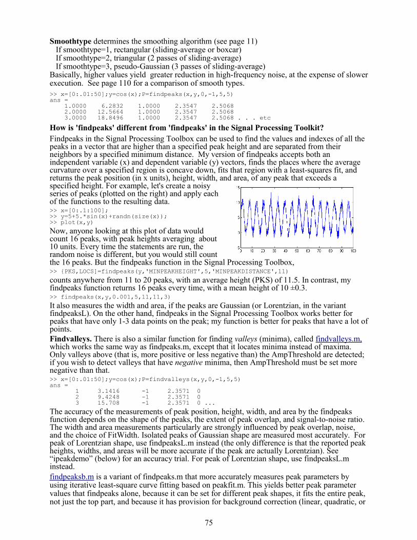
Smoothtype determines the smoothing algorithm (see page 11) If smoothtype=1, rectangular (sliding-average or boxcar) If smoothtype=2, triangular (2 passes of sliding-average) If smoothtype=3, pseudo-Gaussian (3 passes of sliding-average)Basically, higher values yield greater reduction in high-frequency noise, at the expense of slower execution. See page 110 for a comparison of smooth types.>> x=[0:.01:50];y=cos(x);P=findpeaks(x,y,0,-1,5,5)ans = 1.0000 6.2832 1.0000 2.3547 2.5068 2.0000 12.5664 1.0000 2.3547 2.5068 3.0000 18.8496 1.0000 2.3547 2.5068 . . . etc

How is 'findpeaks' different from 'findpeaks' in the Signal Processing Toolkit?Findpeaks in the Signal Processing Toolbox can be used to find the values and indexes of all the peaks in a vector that are higher than a specified peak height and are separated from their neighbors by a specified minimum distance. My version of findpeaks accepts both an independent variable (x) and dependent variable (y) vectors, finds the places where the average curvature over a specified region is concave down, fits that region with a least-squares fit, and returns the peak position (in x units), height, width, and area, of any peak that exceeds a specified height. For example, let's create a noisy series of peaks (plotted on the right) and apply each of the functions to the resulting data.>> x=[0:.1:100];>> y=5+5.*sin(x)+randn(size(x));>> plot(x,y)

Now, anyone looking at this plot of data would count 16 peaks, with peak heights averaging about 10 units. Every time the statements are run, the random noise is different, but you would still count the 16 peaks. But the findpeaks function in the Signal Processing Toolbox,>> {PKS,LOCS]=findpeaks(y,'MINPEAKHEIGHT',5,'MINPEAKDISTANCE',11)

counts anywhere from 11 to 20 peaks, with an average height (PKS) of 11.5. In contrast, my findpeaks function returns 16 peaks every time, with a mean height of 10 ±0.3. >> findpeaks(x,y,0.001,5,11,11,3)

It also measures the width and area, if the peaks are Gaussian (or Lorentzian, in the variant findpeaksL). On the other hand, findpeaks in the Signal Processing Toolbox works better for peaks that have only 1-3 data points on the peak; my function is better for peaks that have a lot of points. Findvalleys. There is also a similar function for finding valleys (minima), called findvalleys.m, which works the same way as findpeaks.m, except that it locates minima instead of maxima. Only valleys above (that is, more positive or less negative than) the AmpThreshold are detected; if you wish to detect valleys that have negative minima, then AmpThreshold must be set more negative than that.>> x=[0:.01:50];y=cos(x);P=findvalleys(x,y,0,-1,5,5)ans = 1 3.1416 -1 2.3571 0 2 9.4248 -1 2.3571 0 3 15.708 -1 2.3571 0 ...

The accuracy of the measurements of peak position, height, width, and area by the findpeaks function depends on the shape of the peaks, the extent of peak overlap, and signal-to-noise ratio. The width and area measurements particularly are strongly influenced by peak overlap, noise, and the choice of FitWidth. Isolated peaks of Gaussian shape are measured most accurately. For peak of Lorentzian shape, use findpeaksL.m instead (the only difference is that the reported peak heights, widths, and areas will be more accurate if the peak are actually Lorentzian). See “ipeakdemo” (below) for an accuracy trial. For peak of Lorentzian shape, use findpeaksL.m instead. findpeaksb.m is a variant of findpeaks.m that more accurately measures peak parameters by using iterative least-square curve fitting based on peakfit.m. This yields better peak parameter values that findpeaks alone, because it can be set for different peak shapes, it fits the entire peak, not just the top part, and because it has provision for background correction (linear, quadratic, or

75

flat). This function works best with isolated peaks that do not overlap. For version 3, the syntax is P = findpeaksb(x,y, SlopeThreshold, AmpThreshold, smoothwidth, peakgroup, smoothtype, windowspan, PeakShape, extra, autozero). The first seven input arguments are exactly the same as for the findpeaks.m function; if you have been using findpeaks or iPeak to find and measure peaks in your signals, you can use those same input argument values for findpeaksb.m. The remaining four input arguments of are for the peakfit function: "windowspan" specifies the number of data points over which each peak is fit to the model shape (it must be large enough to cover the entire peak and get down to the background on both sides of the peak); "PeakShape" specifies the model peak shape (1=Gaussian, 2=Lorentzian, etc), "extra" is the shape modifier variable for the Voigt, Pearson, exponentially broadened Gaussian and Lorentzian, Gaussian/Lorentzian blend, and bifurcated Gaussian and Lorentzian shapes to fine-tune the peak shape; “autozero” is 0, 1, 2, or 3 for no, linear, quadratic, or flat background subtraction. The peak table returned by the function has a 6th column listing the percent fitting errors for each peak. This example, of three Gaussian peaks on a linear background, illustrates the accuracy advantages of this function over findpeaks.m:x=1:.2:100;Heights=[1 2 3];Positions=[20 50 80];Widths=[3 3 3];y=2-(x./50)+modelpeaks(x,3,1,Heights,Positions,Widths)+.02*randn(size(x));plot(x,y);disp(' Peak Position Height Width Area % error')PlainFindpeaks=findpeaks(x,y,.00005,.3,15,15,3)NoBackgroundSubtraction=findpeaksb(x,y,.00005,.5,30,20,3,150,1,0)LinearBackgroundSubtraction=findpeaksb(x,y,.00005,.5,30,20,3,150,1,1)

findpeaksb3.m is a variant of findpeaksb.m that fits each detected peak along with the previous and following peaks found by findpeaks.m, so as to deal better with overlapping peaks. Type “help findpeaksb3.m” for syntax and examples. See this example graphic.

findpeaks plot.m is a simple variant of findpeaks.m that also plots the x,y data and numbers the peaks on the graph (if any are found).

FindpeaksE.m is a variant of findpeaks.m that additionally estimates the percent relative fitting error of each peak (assuming a Gaussian peak shape) and returns it in the 6th column of the peak table. Example: x=[0:.01:5];findpeaksnr(x,x.*sin(x.^2).^2+.1*whitenoise(x),.001,1,15,10)

Peak start and end. Defining the "start" and "end" of the peak (the x-values where the peak begins and ends), is a bit arbitrary because typical peak shapes approach the baseline asymptotically far from the peak maximum. You might define the peak start and end points as where the y values is low, say, 1% of the peak height. But then the random noise on the baseline will often be a large fraction of the signal amplitude at that point. Smoothing to reduce noise is known to distort and broaden peaks, effectively changing their start and end points. One solution is to fit each peak to a model shape, then calculate the peak start and end from the model expression. That minimizes the noise problem by fitting the data over the entire peak, but it works only if the peaks can be accurately modeled by available fitting programs. For example, Gaussian peaks reach a fraction a of the peak height of x=p±sqrt(w^2 log(1/a))/(2 sqrt (log(2))) where p is the peak position and w is the peak width. So, for example if a=.01 (that is, 1%), x=p±1.288784*w. Lorentzian peaks reach a fraction a of the peak height of x=p±sqrt[(w^2 - a w^2)/a]/2. If a=.01, x=p±4.97493*w. The findpeaks variants findpeaksGSS.m and findpeaksLSS.m, for Gaussian and Lorentzian peaks respectively, compute the 1% peak start and end positions in this manner and return them in the 6th and 7th columns of the peak table.findpeaksfit.m is a findpeaks variant that is essentially a serial combination of findpeaks.m and peakfit.m. It uses the number of peaks found and the peak positions and widths determined by findpeaks as input for the peakfit.m function, which then fits the entire signal with the specified peak model. This yields better values that findpeaks alone, because peakfit fits the entire peak, not just the top part, and it deals with non-Gaussian and overlapped peaks. But, it fits only those peaks that are found by findpeaks. peakstats.m uses the same algorithm as findpeaks.m, but it computes and returns a table of summary statistics of the peak intervals (the x-axis interval between adjacent detected peaks), heights, widths, and areas, listing the maximum, minimum, average, and percent standard deviation of each, and optionally plotting the x,y data with numbered peaks in figure window 1, printing the table of peak statistics in the command window, and plotting histograms of the peak

76

intervals, heights, widths, and areas in figure window 2.>> x=[0:.1:1000];y=5+5.*cos(x)+randn(size(x));PS=peakstats(x,y,0,-1,15,23,3,1);Peak Summary Statistics15 peaks detected Interval Height Width AreaMaximum 6.6552 10.7393 4.2968 47.1482Minimum 5.8525 9.5884 2.2744 26.0028Mean 6.272 10.1845 3.0942 33.4194% STD 3.1852 3.4479 18.3062 16.5684

Demo scripts: DemoFindPeak.m and DemoFindPeaksb.mThese are demonstration scripts using the findpeaks and findpeaksb functions on noisy synthetic peak data. They number the peaks and print out the P matrix in the Matlab/Octave command window. He difference between them is that DemoFindPeaksb.m uses findpeaksb, which has the ability to correct for background. (The findpeaks function would not give accurate measurements of peak height, width, and area for this signal, because it does not correct for background). Demo FindPeak S NR is a variant of DemoFindPeak.m that uses

findpeaksnr.m to compute the signal-to-noise ratio (SNR) of each peak and returns it in the 5th column.

Using the peak table matrix. The above functions return the peak table as a matrix, in the order peak number, position, height, width, (and, for findpeaksb.m, the percent fitting error), which you can assign to a variable (e.g. P) and then use Matlab/Octave functions to extract specific information from that matrix. For example:[P(:,2) P(:,3)] is the time series of peak heights (peak position in the 1st column and peak height in the 2nd column); mean(P(:,3)) returns the average peak height (because peak height is in the 3rd column); max(P(:,3)) returns the maximum peak height; hist(P(:,3)) displays the histogram of peak heights; std(P(:,4))/mean(P(:,4)) returns the relative standard deviation of the peak widths (column 4); for n=1:length(P)-1;d(n)=max(P(n+1,2)-P(n,2));end creates "d" as the vector of x-axis distance between peaks. Using my downloadable val2ind.m function: val2ind(P(:,3),7.5) returns the peak number of the peak whose height is closest to 7.5; P(val2ind(P(:,2),18.85),3) returns the peak height (3rd column) whose position (2nd column) is closest to 18.85; and so on.

Peak Identification The command line function idpeaks.m is used for identifying peaks according to their x-axis maximum positions. The syntax is [IdentPeaks,AllPeaks]=idpeaks(M,AmpT,SlopeT,sw,fw,maxerror,Positions,Names)

It finds peaks in the signal “M” (x-values in column 1 and y-values in column 2), according to the peak detection parameters AmpT, SlopeT, sw, fw (see the “findpeaks” function above), then compares the found peak positions (x-values) to a database of known peaks, in the form of an array of known peak maximum positions (“Positions”) and matching cell array of names (“Names”). If the position of a peak found in the signal is closer to one of the known peaks by less than the specified maximum error “maxerror”, that peak is considered a match and its peak position, name, error, and peak amplitude (height) are entered into the output cell array “IdentPeaks”. The full list of detected peaks, identified or not, is returned in “AllPeaks”. You can use “cell2mat” to access numeric elements of IdentPeaks, e.g. cell2mat(IdentPeaks(2,1)) returns the position of the first identified peak, cell2mat(IdentPeaks(2,2))returns its name, and so forth for the peak position error and peak height. (The interactive iPeak function, discussed in the next section, also has the same peak identification feature; see page 80). Example: Download idpeaks.zip, extract it, and place the extracted files in the Matlab or Octave path. This contains a high-resolution atomic emission spectrum of copper ('spectrum') and a data table of known Cu I and II atomic lines ('DataTable') containing their positions and names.

>> load DataTable

77

>> load spectrum>> idpeaks(Cu,0.01,.001,5,5,.01,Positions,Names)

ans= 'Position' 'Name' 'Error' 'Amplitude' [ 221.02] 'Cu II 221.027' [ -0.0025773] [ 0.019536] [ 221.46] 'Cu I 221.458' [ -0.0014301] [ 0.4615] [ 221.56] 'Cu I 221.565' [-0.00093125] [ 0.13191]

The lower the settings of the AmpThreshold, SlopeThreshold, and SmoothWidth, the more peaks will be detected; and the higher the setting of "MaxError", the more peaks will be close enough to the reference peaks to be considered identified. Of course, the accuracy of identifi-ation depends on the x-axis calibration of the measuring instrument (e.g. the wavelength accuracy of a spectrometer). For atomic emission or absorption spectroscopy, tables of known atomic lines can be obtained from NIST, the National Institute for Standards and Technology, and from ASTM, the American Society for Testing and Materials. (See reference 47, page 118). Rectangular pulses. Flat-topped pulses require a different approach, based on a simple amplitude threshold rather than differentiation. The function "findsquarepulse.m" (syntax S=findsquarepulse(t,y,threshold) locates the rectangular pulses in the signal t,y that exceed a y-value of "threshold" and determines their start time, average height (relative to the baseline) and width. Returns the start time, height, and width of each pulse. DemoFindsquare.m creates a test signal and calls findsquarepulse.m. The iPeak Function (ipeak .m), version 5.9, for MatlabZIP file available at http://terpconnect.umd.edu/~toh/spectrum/ ipeak 5.zip Animated step-by-step instructions at http://terpconnect.umd.edu/~toh/spectrum/ipeak.html

iPeak is a Matlab keyboard-operated Interactive Peak Finder for time series data, based on the “findpeaks.m” function. It displays the entire signal in the lower half of the Figure window and an adjustable zoomed-in section in the upper window. (Press the Enter key to change the plot color.) Simple keystrokes allow you to adjust the peak detection parameters AmpThreshold (A/Z keys), SlopeThreshold (S/X keys), SmoothWidth (D/C keys), FitWidth (F/V keys), and other controls. (See list of Keyboard Controls, below). This function can be used to determine experimentally what values of those parameters give the most reliable peak detection for a particular type of data, detecting the desired peaks and ignoring those that are too small, too broad, or too narrow to be of interest. Detected peaks are numbered from left to right. Returns the peak table in a matrix (columns: peak #, position, height, width, area, and percent fitting error; one row for each peak detected). Press P to display a labeled peak table of all the detected peaks in the command window. Press Shift-P to save peak table as disc file. EXAMPLE 1: Two input arguments; data in separate x and y vectors >> x=[0:.1:100];y=(x.*in(x)).^2;ipeak(x,y); EXAMPLE 2: One input argument; data in two columns of a matrix >> x=[0:.01:5]';y=x.*in(x.^2).^2;ipeak([x y]) EXAMPLE 3: One input argument; data in single vector >> y=cos(.1:.1:100);ipeak(y) Keystrokes allow you to pan and zoom the upper window, to inspect each peak in detail if desired. You can set the initial values of pan and zoom in optional input arguments 7 ('xcenter') and 8 ('xrange'). See example 6 below.

78

EXAMPLE 4: Additional scalar argument (after the data) to control peak sensitivity. >> x=[0:.1:100];y=5+5.*cos(x)+randn(size(x));ipeak(x,y,10); or >> ipeak([x;y],10); or >> ipeak(humps(0:.01:2),3) or >> x=[0:.1:10];y=exp(-(x-5).^2);ipeak([x' y'],1)The additional argument is an estimate of the ratio of the typical peak width to the length of the entire data record. Small values detect fewer peaks; larger values detect more peaks. It effects only the starting values for the peak detection parameters. (This is just a quick way to set reasonable initial values for the peak detection parameters, rather than specifying each one individually as in the following example). EXAMPLE 5: Six input arguments. As above, but input arguments 3 to 6 directly specify the initial values of PeakD, AmpT, SlopeT, SmoothW, FitW. (PeakD is ignored in this case, so just type a '0' as the second argument after the data atrix). >> ipeak(datamatrix,0,.5,.0001,20,20);

EXAMPLE 6: Eight input arguments. As above, but input arguments 7 and 8 specify the initial pan and zoom settings, 'xcenter' and 'xrange', respectively. In this example, the x-axis data are wavelengths in nanometers (nm), and the upper window zooms in on a very small 0.4 nm region centered on 249.7 nm. (These data, provided in the ZIP file mentioned above, are from a high-resolution atomic spectrum). >> load ipeakdata.mat >> ipeak(Sample1,0,110,0.06,3,4,249.7,0.4);

EXAMPLE 7: Nine input arguments. As example 6, but the 9th input argument controls the baseline correction mode (equivalent to pressing the T key), which can be 0 (none), 1 (linear), 2 (quadratic), or 3 (flat). If not specified, it is 0 (none). >> ipeak(Sample1,0,110,0.06,3,4,249.7,0.4,1);

The Spacebar/Tab keys jump to the next/previous detected peak and displays it in the upper window at the current zoom setting (use the up and down cursor arrow keys to adjust the zoom range). Or you can press the J key to jump directly to a specified peak number. The L key turns off and on peak parameter labeling. The Y key toggles between linear and log y-axis scale in the lower window (a log axis is good for inspecting signals with high dynamic range; it effects only the lower window display and has no effect on the peak detection or measurements). The U key switches between peak and valley detection mode. Shift-G switches between Gaussian and Lorentzian peak modes.

The T key cycles the baseline correction mode through four modes: OFF, linear, quadratic, and flat. When OFF, peak heights are measured relative to zero. (If the peaks are superimposed on a background, use the baseline subtract keys - B and G - first to subtract the background). In linear and quadratic modes, peak heights are automatically measured relative to a calculated baseline that is linearly or quadratically interpolated from the signal at the edges of the signal in the upper window; use the zoom controls to isolate the peaks so that the signal returns to the local baseline between the peaks as displayed in the upper window. (In those modes, the peak heights, widths, and areas in the peak table (R or P keys) will be automatically corrected for the baseline. OFF will give better results when the baseline is zero, or has been subtracted using the B key, even if the peaks are partly overlapped. Linear and quadratic will work best if the peaks are well separated so that the signal returns to the local baseline between the peaks. Flat mode applies only to the curve fitting operation (N and M keys); it corrects for a flat baseline shift even if the signal does not return to the baseline.

Peak summary statistics table. The E key command prints a table of summary statistics of the peak intervals (the x-axis interval between adjacent detected peaks), heights, widths, and areas, listing the maximum, minimum, average, and percent standard deviation, and displaying the histogram of each of these in figure windows 2.

Normal and Multiple Curve fitting: If the peaks are highly overlapped, or if they are not Gaussian in shape, the best results will be obtained by using the curve fitting function - the N or M keys). The N key applies iterative curve fitting to the detected peaks that are displayed in the upper window (referred to here as “Normal” curve fitting). The use of the iterative least-squares

79

function can result in more accurate peak parameter measurements that the normal peak table (R or P keys), especially if the peaks are non-Gaussian in shape or are highly overlapped. If the peaks are superimposed on a background, use the T key to set the baseline correction mode to flat, linear, or quadratic. Then use the pan and zoom keys to select a peak or a group of overlapping peaks in the upper window, with the signal returning all the way to the local baseline at the ends of the upper window. Make sure that AmpThreshold, SlopeThreshold, SmoothWidth are adjusted so that each peak is numbered once. Then press the N key, type a number for the desired peak shape at the prompt in the Command window and press Enter (1=Gaussian (default), 2=Lorentzian, 3=logistic, 4=Pearson, 5=exponentially broadened Gaussian; 6=equal-width Gaussians; 7=Equal-width Lorentzians; 8=exponentially broadened equal-width Gaussian, 9=exponential pulse, 10=sigmoid, 11=Fixed-width Gaussian, 12=Fixed-width Lorentzian; 13=Gaussian/ Lorentzian blend; 14=bifurcated Gaussian; 15=bifurcated Lorentzian); 16=Fixed-position Gaussians; 17=Fixed-position Lorentzians; 18= exponentially broadened Lorentzian; 19=alpha function; 20=Voigt profile, then type in a number of repeat trial fits and press Enter (the default is 1; start with that and then increase if necessary). If you have selected a variable-shape peak (numbers 4, 5, 8 ,13, 14, or 15), the program will ask you to type in a number that controls the shape (“extra” in the peakfit input arguments). The program will then perform the fit, display the results graphically in Figure window 2, and print out a table of results in the command window:Peak shape (1-8): 1 Number of trials: 1Least-squares fit to Gaussian peak model using this peakfit function:>> peakfit(DataMatrix,355,292,3,1,1,1,[225 54 274 55 323 45],0); Fitting Error 0.23243% Peak# Position Height Width Area 2 224.63 214.31 60.949 10106 3 276.35 278.66 47.409 14057 4 324.67 403.88 50.321 21634The use of the iterative least-squares function can result in more accurate peak parameter measurements that the normal peak table (R or P keys), especially if the peaks are non-Gaussian in shape or are highly overlapped.

There is also a “Multiple” peak fit function (M key) that will apply iterative curve fitting to all the detected peaks in the signal simultaneously. Before using this function, it's best to set the baseline mode to 'none' (T key) and use the multi-segment baseline correction function (B key) to remove the background (because the autozero function will probably not be able to subtract the baseline from the entire signal). Then press M and proceed as for the normal curve fit. A multiple curve fit may take a minute or so to complete if the number of peaks is large, possibly longer than the Normal curve fitting function on each group of peaks separately. It will attempt to fit only those peaks that it finds.

The N and M key fitting functions perform non-linear iterative curve fitting (page 54) using the peakfit .m function (page 90). The number of peaks and the starting values of peak positions and widths for the curve fit function are automatically supplied by the findpeaks function, so it is essential that the peak detection variables in iPeak be adjusted so that all the peaks in the selected region are detected and numbered once. (For more flexible curve fitting, use ipf.m, page 95). Pressing the H key may help to detect overlapped peaks.Note 1: If the peaks are too overlapped to be detected and numbered separately, try pressing the H key to activate the sharpen function before pressing M. Note 2: If you plan to use a variable-shape peak (numbers 4, 5, 8 ,13, 14, or 15) for the Multiple peak fit, it's a good idea to obtain a reasonable value for the requested “extra” shape parameter by performing a Normal peak fit on an isolated single peak (or small group of partly-overlapping peaks) of the same shape, then use that value for the Multiple curve fit of the entire signal. Note 3: Although the peak widths can vary from peak to peak, the curve fit routines assume that the peak shape is the same for all peaks in one fitting operation, so if the peak shape varies across the signal, use the Normal peak fit to fit each section with a different shape rather than the Multiple peak fit.

80

Note 4: If the density of data points on the peaks is too low - less than about 4 points - the peaks may not be reliably detected; you can improve reliability by using the interpolation command (Shift-I) to re-sample the data by linear interpolation to a larger number of points. Conversely, if the density of data points on the peaks is very high - say, more than 100 points per peak - then you can speed up the operation of iPeak by re-sampling to a smaller number of points. Peak identification: There is an optional “peak identification” function if optional input arguments 9 (“MaxError”), 10 (“Positions”), and 11 (“Names”) are included. The “i” key toggles this function ON and OFF. This function compares the found peak positions (maximum x-values) to a database of known peaks, in the form of an array of known peak maximum positions (“Positions”) and matching cell array of names (“Names”). If the position of a found peak in the signal is closer to one of the known peaks by less than the specified maximum error (“MaxError”), then that peak is considered a match and its name is displayed next to the peak in the upper window. When the “o” key is pressed, the peak positions, names, errors, and amplitudes are printed out in a table in the command window. EXAMPLE 8: Eleven input arguments. As above, but also specifies “MaxError”, “Positions”, and “Names” in optional input arguments 9, 10, and 11, for peak identification function. Pressing the “i” key toggles off and on the peak identification labels in the upper window. Pressing “o” prints the peak positions, names, errors, and amplitudes in a table in the command window. These data (provided in the ZIP file mentioned above) are from a high-resolution atomic spectrum (x-axis in nanometers). >> load ipeakdata.mat >> ipeak(Sample1,0,120,0.06,3,6,296,5,0.1,Positions,Names);

Note: The ZIP file contains the latest version of the iPeak function as well as some sample data to demonstrate peak identification (Example 7 and 8). Obviously for your own applications, it's up to you to provide your own array of known peak maximum positions ('Positions') and matching cell array of names ('Names') for your particular types of signals.

IPeak 5.96 Keyboard Controls Pan signal left and right...Coarse pan: < and > keys Fine pan: left and right cursor arrow keys Nudge left and right: [ and ] keys Zoom in and out............Coarse zoom: / and ' keys Fine zoom: up and down cursor arrow keys Resets pan and zoom.........ESC Change plot color...........Enter Adjust AmpThreshold.........A,Z (Larger values ignore short peaks) Type in AmpThreshold........Shift-A Adjust SlopeThreshold.......S,X (Larger values ignore broad peaks) Type in SlopeThreshold......Shift-S Adjust SmoothWidth..........D,C (Larger values ignore sharp peaks} Adjust FitWidth.............F,V (Adjust to cover just top part of peaks) Toggle sharpen mode ........H Helps detect overlapped peaks. Baseline correction.........B, then click baseline at multiple points Restore original signal.....G to cancel previous background subtraction Invert signal...............- Invert (negate) the signal (flip + and -) Set minimum to zero.........0 (Zero) Sets minimum signal to zero Interpolate signal..........Shift-I Interpolate (re-sample) to N points Toggle log y mode OFF/ON....Y Plot log Y axis on lower graph Cycles baseline modes.......T 0=none; 1=linear; 2=quadratic; 3=Flat. Toggle valley mode OFF/ON...U Switch between peak and valley modes Gaussian/Lorentzian switch..Shift-G Switch between Gaussian/Lorentzian Print peak table............P Prints Peak #, Position, Height, Width Save peak table.............Shift-P Saves peak table as disc file Step through peaks..........Space/Tab Jumps to next/previous peak Jump to peak number.........J Type peak number and press Enter. Normal peak fit.............N Fit peaks in upper window with peakfit.m Multiple peak fit...........M Fit all peaks in signal with peakfit.m Print keyboard commands.....K Prints this list Print findpeaks arguments...Q Prints findpeaks function with arguments. Print ipeak arguments.......W Prints ipeak function with all arguments. Print report................R Prints Peak table and parameters Print peak statistics.......E prints mean, std of peak intervals, heights... Peak labels ON/OFF......... L Label all peaks detected in upper window. Peak ID ON/OFF..............I Identifies closest peaks in 'Names' database. Print peak IDs..............O Prints table of peaks IDs

81

iPeak Demo functions The ZIP file at http://terpconnect.umd.edu/~toh/spectrum/ ipeak 5.zip contains several demo functions (ipeakdemo.m, ipeakdemo1.m, etc) that illustrate various aspect of the iPeak function and how it can be used effectively. Run them by typing their name at the Matlab command windows prompt.Which to use: iPeak or Peakfit? To help decide, you may wish to download the ZIP file at http://terpconnect.umd.edu/~toh/spectrum/idemos.zip that contains some Matlab demo functions comparing iPeak.m with Peakfit.m for signals with a few peaks and signals with many peaks and that shows how to adjust iPeak to detect broad or narrow peaks. These are self-contained demos that include all required Matlab functions. Just place them in your path and click Run or type their name at the command prompt.

ipeakdemo.m ipeakdemo: effect of the peak detection parametersFour Gaussian peaks with the same heights but different widths (10, 30, 50 and 70 units). This demonstrates the effect of SlopeThreshold and SmoothWidth on peak detection. Increasing SlopeThreshold (S key) will discriminate against the broader peaks. Increasing SmoothWidth (D key) will discriminate against the narrower peaks and noise. FitWidth (F/V keys) controls the number of points around the “top part” of the (unsmoothed) peak that are taken to estimate the peak heights, positions, and widths. A reasonable value is about equal to 1/2 of the number of data points in the half-width of the peaks. In this case, where the peak widths are quite different, set it to about 1/2 of the number of data points in the narrowest peak.

ipeakdemo1.m

ipeakdemo1: the background correction modesDemonstration of background correction, for separated, narrow peaks on a large baseline. A table of the actual peak positions, heights, widths, and areas is printed out in the command window. Jump to the next/previous peaks using the Spacebar/Tab keys. Hint: Use the T key to set the baseline correction mode to “Linear” or “Quadratic”, adjust the zoom setting so that the peaks are shown one at a time in the upper window, then press the P key to display the peak table. (Each time you run this demo, you will get a different set of peaks and noise).

ipeakdemo2.m

ipeakdemo2: peak overlap and the curve fitting functions. Demonstration of error caused by overlapping peaks on a large offset baseline. A table of the actual peak positions, heights, widths, and areas is printed out in the command window. Jump to the next/previous peaks using the Spacebar/Tab keys. Hint: Use the B key and click on the baseline points, then press the P key to display the peak table. Or turn on the baseline correction mode (T key) and use the Normal curve fit (N key) or Multiple curve fit (M key). (Each time you run this demo, you will get a different set of peaks and noise).

ipeakdemo3.m

ipeakdemo3: Non-Gaussian peak shapes Demonstration of overlapping Lorentzian peaks, without an added background. Overlap of peaks causes significant errors in peak height, width, and area. Jump to the next/previous peaks using the Spacebar/Tab keys. Each time you run this demo, you will get a different set of noise. A table of the actual peak positions, heights, widths, and areas is printed out in the command window. Hint: Press Shift-G to switch to Lorentzian mode; set the baseline correction mode to OFF (T key) and use the Normal curve fit (N key) with peak shape 2 (Lorentzian).

82

240 260 280 300 320 340

0

1

2

3

4

iPeak 3.5. Autozero ON. Press K for keyboard commands 4

8

11

1314 15

16

18

Peak 1Position: 300.4918Height: 3.9459Width: 27.9814

500 1000 1500 2000 2500 3000 3500 4000

5

10

15

Adjustment Keys: AmpT: A/Z SlopeT: S/X SmoothWidth: D/C FitWidth: F/V

Line

ar m

ode

AmpT: 0.89678 SlopeT: 0.00077778 SmoothW: 15 FitW: 15

1

2

3

4

5 6

7

8

9

10

11

12

13 141516

17

18

40 60 80 100 120 140 160

0

0.5

1

iPeak 3.5. Autozero OFF. Press K for keyboard commands

1

Peak 1Position: 100.1629Height: 0.93683Width: 13.1152

100 200 300 400 500 600 700 800 900 1000 1100 12000

5

10

Adjustment Keys: AmpT: A/Z SlopeT: S/X SmoothWidth: D/C FitWidth: F/V

Line

ar m

ode

AmpT: 0.54237 SlopeT: 0.00066272 SmoothW: 16 FitW: 16

1 2

3 4

5 6

7 8

9 10

40 60 80 100 120 140 160

0.2

0.4

0.6

0.8

1

iPeak 3.5. Autozero OFF. Press K for keyboard commands

1 2 3 4Peak 1Position: 100Height: 1Width: 10.0004

50 100 150 200 250 300 350 400 450 500

0.2

0.4

0.6

0.8

1Adjustment Keys: AmpT: A/Z SlopeT: S/X SmoothWidth: D/C FitWidth: F/V

Line

ar m

ode

AmpT: 0.050175 SlopeT: 0.0004375 SmoothW: 20 FitW: 20

1 2 3 4

400 420 440 460 480 500 520 540 560 580

6

8

10

iPeak 3.5. Autozero OFF. Press K for keyboard commands

1

2 3

4 5

6

7

8

9 10

11

12

13

14

15

16

17

Peak 1Position: 500.0927Height: 10.7729Width: 81.856

500 1000 1500 2000 2500 3000 3500 4000

2

4

6

8

10

Adjustment Keys: AmpT: A/Z SlopeT: S/X SmoothWidth: D/C FitWidth: F/V

Line

ar m

ode

AmpT: 0.53983 SlopeT: 0.00019444 SmoothW: 30 FitW: 30

1

2 3

4 5

6

7

8

910

11

12

13

14

15

1617

ipeakdemo4.m

ipeakdemo4: dealing with very noisy signalsDetection and measurement of four peaks in a very noisy signal. The signal-to-noise ratio of first peak is 2. A table of the actual peak positions, heights, widths, and areas is printed out in the command window. Jump to the next/previous peaks using the Spacebar/Tab keys. The peak at x=100 is usually detected, but the accuracy of peak parameter measurement is poor because of the low signal-to-noise ratio. Hint: Increase SmoothWidth and FitWidth to help reduce the effect of the noise. Each time you run this demo, you will get a different set of noise.

ipeakdemo5.m

ipeakdemo5: dealing with highly overlapped peaksIn this demo the peaks are so highly overlapped that only one or two of the highest peaks yield distinct maxima that are detected by iPeak. The height, width, and area estimates are highly inaccurate because of this overlap. The normal peak fit function ('N' key) would be useful in this case, but it depends on iPeak for the number of peaks and for the initial guesses, and so it would fit only the peaks that were found and numbered. To help in this case, pressing the 'H' key will activate the peak sharpen function that decreases peak width and increases peak height of all the peaks, making it easier for Findpeaks to detect and number them for use by the peakfit function. Note: peakfit fits the original unmodified peaks; the sharpening is used only to help locate the peaks.

Note: The ZIP file available at http://terpconnect.umd.edu/~toh/spectrum/ ipeak 5.zip contains findpeaks, DemoFindPeaks, ipeak.m, all the ipeakdemos described above, and the ipeakdata.mat file with the high-resolution atomic spectrum used in example 8.

Peak Finding and Measurement Spreadsheet

The spreadsheet pictured above implements the "findpeaks" peak finding and measurement method in a spreadsheet. The input x,y data are contained in Sheet1, column A and B, rows 8 to 263. You can Copy and Paste your own data there. The amplitude threshold and slope threshold are set in cells B3 and E3, respectively.

Smoothing and differentiation are performed by the convolution technique used by the spreadsheet DerivativeSmoothing.xls described previously. The Smooth Width and the Fit Width are both controlled by the number of non-zero convolution coefficients in row 5, columns J through Z. (In order to compute a symmetrical first derivative, the coefficients in columns J to

83

40 60 80 100 120 140 160

-1

0

1

2iPeak 3.5. Autozero OFF. Press K for keyboard commands

1

2

3

Peak 1Position: 99.6398Height: 1.0711Width: 21.5707

50 100 150 200 250 300 350 400 450 500

0

2

4

Adjustment Keys: AmpT: A/Z SlopeT: S/X SmoothWidth: D/C FitWidth: F/V

Line

ar m

ode

AmpT: 0.21827 SlopeT: 0.00077778 SmoothW: 30 FitW: 30

12

34

Q must be the negatives of the positive coefficients in columns S to Z). The original data and the smoothed derivative are shown in the two charts on Sheet1.

To detect peaks in the data, a series of three conditions are tested for each data point in columns F, G, and H, corresponding to the three nested loops in findpeaks.m:

1. Is the signal greater than Amplitude Threshold? (line 45 of findpeaks.m; column F in the spreadsheet)

2. Is there a downward directed zero crossing in the smoothed first derivative? (line 43 of findpeaks.m; column G in the spreadsheet)

3. Is the slope of the derivative at that point greater than the Slope Threshold? (line 44 of findpeaks.m; column H in the spreadsheet)

If the answer to all three questions is yes (highlighted by blue cell coloring), a peak is registered at that point (column I), counted in column J, and assigned an index number in column K.

For the first 10 peaks found, the x,y original unsmoothed data are copied to Sheet2 through Sheet11, where that segment of data is subjected to a Gaussian least-squares fit, using the technique described on page 43. The best-fit Gaussian parameter results are copied back to Sheet1, in the table in columns AH-AK. (In its present form, the spreadsheet is limited to measuring 10 peaks, although it can detect any number of peaks. It's also limited in Smooth Width and Fit Width by the 17-point convolution coefficients).

This spreadsheet is available in OpenOffice (.ods) and in Excel (.xls) and (.xlsx) formats. They are functionally equivalent and differ only in minor cosmetic aspects. An example spreadsheet, with data, is available. A demo version, with a calculated noisy waveform that you can modify, is also available. Download from http://tinyurl.com/cey8rwh.

To expand this spreadsheet to larger numbers of data points, simply drag down row 263, columns A through K, so that the formulas in those rows are replicated for the required number of additional rows, then adjust the charts to accommodate the extra rows. Expanding the spreadsheet to larger numbers of measured peaks is more difficult: (1) drag down row 17, columns AC through AK, and adjust the formulas in those rows for the required number of additional peaks; (2) copy all of Sheet11 and paste it into a series of new sheets (Sheet12, Sheet13, etc), one for each additional peak; (3) adjust the formulas in columns B and C in each of these additional sheets to refer to the appropriate row in Sheet1; (4) carefully modify these additional equations in the added sheets, using the same pattern as those for peaks 1-10.

A comparison of this spreadsheet to its Matlab/Octave equivalent “findpeaksplot.m” is instructive. On the positive side, the spreadsheet literally "spreads out" the data and the calculations spatially over a large number of cells and sheets, breaking down the discrete steps in a very graphic way. In particular, the use of conditional formatting in columns F through K make the peak detection decision process more evident for each peak, and the least-squares sheets 2 through 11 lay out every detail of those calculations. Spreadsheet programs have many flexible formatting options to make displays more attractive.

On the down side, a spreadsheet as complicated as this one is far more difficult to construct than its Matlab/Octave equivalent. Much more serious, the spreadsheet is less flexible and harder to expand to larger signals and larger number of peaks. In contrast, the Matlab/Octave equivalent, while requiring some understanding of programming to construct initially, is faster in operation, more flexible, can easily handle signals and smooth/fit widths of any size, and can detect and measure any number of peaks. Moreover, because it is written as a Matlab/Octave function, it can readily be employed as an element in your own custom Matlab/Octave programs to perform even larger tasks.

84

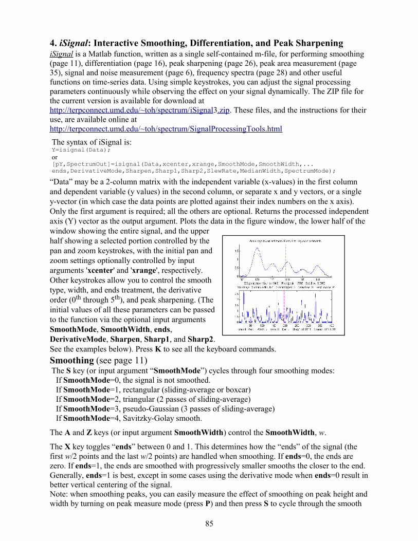
4. iSignal: Interactive Smoothing, Differentiation, and Peak Sharpening iSignal is a Matlab function, written as a single self-contained m-file, for performing smoothing (page 11), differentiation (page 16), peak sharpening (page 26), peak area measurement (page 35), signal and noise measurement (page 6), frequency spectra (page 28) and other useful functions on time-series data. Using simple keystrokes, you can adjust the signal processing parameters continuously while observing the effect on your signal dynamically. The ZIP file for the current version is available for download at http://terpconnect.umd.edu/~toh/spectrum/ iSignal3.zip. These files, and the instructions for their use, are available online at http://terpconnect.umd.edu/~toh/spectrum/SignalProcessingTools.html

The syntax of iSignal is:Y=isignal(Data);or[pY,SpectrumOut]=isignal(Data,xcenter,xrange,SmoothMode,SmoothWidth,... ends,DerivativeMode,Sharpen,Sharp1,Sharp2,SlewRate,MedianWidth,SpectrumMode);

“Data” may be a 2-column matrix with the independent variable (x-values) in the first column and dependent variable (y values) in the second column, or separate x and y vectors, or a single y-vector (in which case the data points are plotted against their index numbers on the x axis). Only the first argument is required; all the others are optional. Returns the processed independent axis (Y) vector as the output argument. Plots the data in the figure window, the lower half of the window showing the entire signal, and the upper half showing a selected portion controlled by the pan and zoom keystrokes, with the initial pan and zoom settings optionally controlled by input arguments 'xcenter' and 'xrange', respectively. Other keystrokes allow you to control the smooth type, width, and ends treatment, the derivative order (0th through 5th), and peak sharpening. (The initial values of all these parameters can be passed to the function via the optional input arguments SmoothMode, SmoothWidth, ends, DerivativeMode, Sharpen, Sharp1, and Sharp2. See the examples below). Press K to see all the keyboard commands.

Smoothing (see page 11) The S key (or input argument “SmoothMode”) cycles through four smoothing modes: If SmoothMode=0, the signal is not smoothed. If SmoothMode=1, rectangular (sliding-average or boxcar) If SmoothMode=2, triangular (2 passes of sliding-average) If SmoothMode=3, pseudo-Gaussian (3 passes of sliding-average) If SmoothMode=4, Savitzky-Golay smooth.

The A and Z keys (or input argument SmoothWidth) control the SmoothWidth, w.

The X key toggles “ends” between 0 and 1. This determines how the “ends” of the signal (the first w/2 points and the last w/2 points) are handled when smoothing. If ends=0, the ends are zero. If ends=1, the ends are smoothed with progressively smaller smooths the closer to the end. Generally, ends=1 is best, except in some cases using the derivative mode when ends=0 result in better vertical centering of the signal.Note: when smoothing peaks, you can easily measure the effect of smoothing on peak height and width by turning on peak measure mode (press P) and then press S to cycle through the smooth

85

modes. There are two special functions for removing or reducing sharp spikes in signals: the M key, which implements a median filter (it asks you to enter the spike width, e.g. 1, 2, 3... points). The ~ key limits the maximum rate of change (slew rate), which can reduce the amplitude of sharp spikes and steps.

Differentiation (see page 17)The D / Shift-D keys (or optional input argument “DerivativeMode”) increase/decrease the derivative order. The default is 0. Careful optimization of smoothing of derivatives is critical for acceptable signal-to-noise ratio.

Peak sharpening or resolution enhancement (see page 26)The E key (or optional input argument “Sharpen”) turns off and on peak sharpening (resolution enhancement). The sharpening strength is controlled by the F and V keys (or optional input argument “Sharp1”) and B and G keys (or optional argument “Sharp2”). The optimum values depend on the peak shape and width. For peaks of Gaussian shape, a reasonable value for Sharp1 is PeakWidth2/25 and for Sharp2 is PeakWidth4/800 (or PeakWidth2/6 and PeakWidth4/700 for Lorentzian peaks), where PeakWidth is the full-width at half maximum of the peaks expressed in number of data points. However, you don't need to do the math yourself; iSignal 1.6 and later can calculate sharpening and smoothing settings for Gaussian and for Lorentzian peak shapes using the Y and U keys, respectively. Just isolate a single typical peak in the upper window using the pan and zoom keys, then press Y for Gaussian or U for Lorentzian peaks. (The optimum settings depends on the width of the peak, so if your signal has peaks of widely different widths, one setting will not be optimum for all the peaks).

You can fine-tune the sharpening with the F/V and G/B keys and the smoothing with the A/Z keys. You can expect a decrease in peak width (and corresponding increase in peak height) of about 20% - 50%, depending on the shape of the peak (the peak area is largely unchanged). Excessive sharpening leads to baseline artifacts and increased noise. iSignal allows you to experimentally determine the values of these parameters that give the best trade-off between sharpening, noise, and baseline artifacts, for your purposes. You can easily measure the effect of sharpening on peak width by turning on peak measure mode (press P) and then press E to toggle the sharpen mode off and on.

Signal measurementThe cursor keys control the position of the green cursor and the dotted red cursors that mark the selected range displayed in the upper graph window. The label under the top graph window shows the value of the signal (y) at the green cursor, the peak-to-peak (min and max) signal range, the area under the signal, and the standard deviation within the selected range (the dotted cursors). Pressing the Q key prints out a table of the signal information in the command window.

Background correctionBackground (or baseline) correction is important because the peak heights, widths, and areas measured by the Peak Measure (P) command are based on the assumption that the baseline under the peaks is zero. There are two methods: manual and automatic. The Backspace key starts manual background correction operation. In the command window, type in the number of background points to click and press the Enter key. The cursor changes to cross hairs; click along the presumed background, starting to the left of the x axis and placing the last click to the right of the x axis. When the last point is clicked, the linearly interpolated baseline between those points is subtracted from the signal. To restore the original background (i.e. to correct an error or to try again), press the '\' key (just below the backspace key).

To select the automatic baseline correction, press the T key repeatedly; it cycles thorough four modes: No baseline correction, linear, quadratic, and flat mode. In linear mode, a straight-line

86

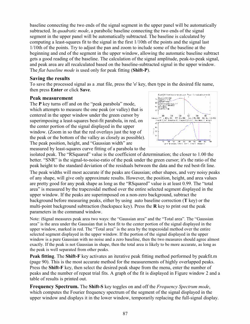
baseline connecting the two ends of the signal segment in the upper panel will be automatically subtracted. In quadratic mode, a parabolic baseline connecting the two ends of the signal segment in the upper panel will be automatically subtracted. The baseline is calculated by computing a least-squares fit to the signal in the first 1/10th of the points and the signal last 1/10th of the points. Try to adjust the pan and zoom to include some of the baseline at the beginning and end of the segment in the upper window, allowing the automatic baseline subtract gets a good reading of the baseline. The calculation of the signal amplitude, peak-to-peak signal, and peak area are all recalculated based on the baseline-subtracted signal in the upper window. The flat baseline mode is used only for peak fitting (Shift-P).

Saving the resultsTo save the processed signal as a .mat file, press the 'o' key, then type in the desired file name, then press Enter or click Save.

Peak measurementThe P key turns off and on the “peak parabola” mode, which attempts to measure the one peak (or valley) that is centered in the upper window under the green cursor by superimposing a least-squares best-fit parabola, in red, on the center portion of the signal displayed in the upper window. (Zoom in so that the red overlays just the top of the peak or the bottom of the valley as closely as possible). The peak position, height, and “Gaussian width” are measured by least-squares curve fitting of a parabola to the isolated peak. The “RSquared” value is the coefficient of determination; the closer to 1.00 the better. “SNR” is the signal-to-noise-ratio of the peak under the green cursor; it's the ratio of the peak height to the standard deviation of the residuals between the data and the red best-fit line.The peak widths will most accurate if the peaks are Gaussian; other shapes, and very noisy peaks of any shape, will give only approximate results. However, the position, height, and area values are pretty good for any peak shape as long as the “RSquared” value is at least 0.99. The “total area” is measured by the trapezoidal method over the entire selected segment displayed in the upper window. If the peaks are superimposed on a non-zero background, subtract the background before measuring peaks, either by using auto baseline correction (T key) or the multi-point background subtraction (backspace key). Press the R key to print out the peak parameters in the command window.

Note: iSignal measures peak area two ways: the “Gaussian area” and the “Total area”. The “Gaussian area” is the area under the Gaussian that is best fit to the center portion of the signal displayed in the upper window, marked in red. The “Total area” is the area by the trapezoidal method over the entire selected segment displayed in the upper window. If the portion of the signal displayed in the upper window is a pure Gaussian with no noise and a zero baseline, then the two measures should agree almost exactly. If the peak is not Gaussian in shape, then the total area is likely to be more accurate, as long as the peak is well separated from other peaks.

Peak fitting. The Shift-F key activates an iterative peak fitting method performed by peakfit.m (page 90). This is the most accurate method for the measurements of highly overlapped peaks. Press the Shift-F key, then select the desired peak shape from the menu, enter the number of peaks and the number of repeat trial fits. A graph of the fit is displayed in Figure window 2 and a table of results is printed out.

Frequency Spectrum. The Shift-S key toggles on and off the Frequency Spectrum mode, which computes the Fourier frequency spectrum of the segment of the signal displayed in the upper window and displays it in the lower window, temporarily replacing the full-signal display.

87

Pan and zoom to adjust the region of the signal to be viewed. Shift-A cycles through four plot modes (linear, semilog X, semilog Y, or log-log) and Shift-X toggles between a frequency on the x axis and time on the x-axis. The frequency (or time) and the harmonic number of the largest component of the spectrum is displayed on the left. All signal processing functions remain active in the frequency spectrum mode (smooth, derivative, etc) so you can observe the effect of these functions on the frequency spectrum of the signal. Click here for an animated example. Press Shift-S again to return to the normal mode. To save the spectrum as a new variable, call iSignal with output arguments [pY,SpectrumOut] and set the 13th input argument 'SpectrumMode' to 1. Version 3 adds the Shift-W command to display the 3D waterfall spectrum, useful for signals whose frequency spectrum varies over the duration of the signal.

Other keystroke controls. The L key toggles off and on the Overlay mode, which overlays the current processed signal with the original signal as a dotted line, for the purposes of comparison. The tab key restores the original signal and cursor settings. The “-” (minus sign) key is used to negate the signal (flip + for -). Press H to toggle the display between a linear y and semilog y plot in the lower window, which is useful for signals with very wide dynamic range (zero and negative points are ignored in the log plot). The 0 key (number 0) removes offset from the signal; sets minimum y value to zero. The semicolon (;) key sets the selected region (between the dotted red cursor lines) to zero; use it to remove uninteresting regions of the signal. The C key condenses the signal by the specified factor n, replacing each group of n points with their average, prompts the user to enter the value of n. (typically, 2,3, 4, etc). The I key replaces the signal with a linearly interpolated version containing m data points, prompts the user to enter the value of m. This can be used to increase or decrease the sampling density or to change an unevenly sampled signal to an evenly sampled one. In version 2.96 you can press Shift-C, then click on the graph to print out the x,y coordinates of that point. This works on both the upper and lower panels, and on the frequency spectrum as well. In Version 3.2, Shift-P plays the the signal segment in the upper panel as audio via computer's sound output (you can type a sample rate or just press Enter for the default sample rate of 8kHz)EXAMPLE 1: Single input argument; data in two columns [x;y] or in a single y vector >> isignal(y); >> isignal([x;y]);EXAMPLE 2: Two input arguments. Data in separate x and y vectors. >> isignal(x,y);

EXAMPLE 3: Three or four input arguments. The last two arguments specify the initial values of pan (xcenter) and zoom (xrange) in the last two input arguments. Using data in the ZIP file: >> load data.mat >> isignal(DataMatrix,180,40); or >> isignal(x,y,180,40);

EXAMPLE 4: As above, but additionally specifies initial values of SmoothMode, SmoothWidth, ends, and DerivativeMode in the last four input arguments. >> isignal(DataMatrix,180,40,2,9,0,1);

EXAMPLE 5: As above, but additionally specifies initial values of the peak sharpening parameters Sharpen, Sharp1, and Sharp2 in the last three input arguments. Press the E key to toggle sharpening on and off for comparison. >> isignal(DataMatrix,180,40,2,9,0,0,1,51,6000);

EXAMPLE 6: Using the built-in “humps” function: >> x=[0:.005:2];y=humps(x);Data=[x;y];4th derivative of the peak at x=0.9: >> isignal(Data,0.9,0.5,1,3,1,4);Peak sharpening applied to the peak at x=0.3:

88

>> isignal(Data,0.3,0.5,1,3,1,0,1,220,5400);Press 'E' key to toggle sharpening ON/OFF to compare)EXAMPLE 7: Measurement of peak area. >> x=[0:.01:20]; >> y=exp(-(x-4).^2)+exp(-(x-9).^2)+exp(-(x-13).^2)+exp(-(x-15).^2); >> isignal(x,y); This example generates four Gaussian peaks with the exact same peak height (1.00) and area (1.77). The first peak (at x=4) is isolated, the second peak (x=9) is slightly overlapped with the third one, and the last two peaks (at x= 13 and 15) are strongly overlapped. To measure the area under a peak using the perpendicular drop method, position the dotted red marker lines straddling the peak at the minimum of the valley between the overlapped peaks.

EXAMPLE 8: Measurement of single peak with random noise spikes. Compare smoothing vs spike filter (M key). Alternatively, use the slew rate limit (~ key) to reduce spike amplitude.>> x=-5:.01:5;>> y=exp(-(x).^2);for n=1:1000,if randn()>2,y(n)=rand()+y(n);,end,end;>> isignal(x,y);

iSignal 3.2 keyboard controls Pan left and right........... Coarse pan: < and > Fine pan: left and right cursor arrows Nudge one point left or right: [ and ]

Zoom in and out.............. Coarse zoom: / and " Fine zoom: up and down cursor arrows Reset pan and zoom........... ESC (resets to initial default values) Adjust smooth width.......... A,Z (A=>more smoothing, Z=>less smoothing) Adjust smooth type........... S (Cycles through None, Rectangular, Triangle, Gaussian, Savitzky-Golay) Toggle smooth ends........... X Flips between 0=ends zeroed 1=ends smoothed Adjust derivative order...... D/Shift-D (Increase/Decrease derivative order) Toggle peak sharpening....... E (flips between 0=OFF 1=ON) Sharpening for Gaussian...... Y Set sharpen settings for Gaussians Sharpening for Lorentzian.... U Set sharpen settings for Lorentzians Adjust sharp1................ F,V F=>sharper, V=>less sharpening Adjust sharp2................ G,B G=>sharper, B=>less sharpening Slew rate limit (0=OFF)...... ~ Largest allowed y change between points Spike filter width (0=OFF)... M spike filter eliminates sharp spikes Toggle peak labeling......... P Labels center peak in upper window Fits peak in upper window.... Shift-F (Asks for shape, number of peaks, etc) Toggle Spectrum mode on/off.. Shift-S (Shift-A and Shift-X to change axes) Display Waterfall spectrum....Shift-W in mesh, surf, contour, or pcolor form Click graph to print out x,y..Shift-C Click graph to print coordinates Toggle overlay mode.......... L Overlays original signal in upper window Toggle log y mode............ H Display semilog y plot in lower window Select baseline mode......... T none, linear, quadratic, or flat baseline mode Restores original signal..... Tab key resets to original signal and modes Baseline subtraction......... Backspace, then click baseline at 8 points Restore background........... \ to cancel previous background subtraction Invert signal................ - Invert (negate) the signal (flip + and -) Remove offset................ 0 (zero) set minimum signal) to zero Trim region to zero.......... ; sets selected region to zero. Absolute value................+ Computes absolute value of entire signal Condense signal.............. C Condense oversampled signal by factor of N Interpolate signal........... i Interpolate (re-sample) to N points Print keyboard commands...... K prints this list Print signal report.......... Q prints signal info and current settings Print iSignal arguments...... W prints iSignal (with current arguments) Save output to disk.......... O Save .mat file containing processed signal Play signal as sound..........Shift-P Play signal in the upper panel through computer sound system (type in sample rate).

89

5. Peak Fitter This section describes Matlab and Octave peak fitting program for time-series signals that uses an unconstrained non-linear optimization algorithm (Page 54). The objective is to determine whether your signal can be represented as the sum of fundamental underlying peaks shapes. The program accepts signals of any length, including those with non-integer and non-uniform x-values and fits any number of peaks at a time with 20 selectable peak shapes (expandable to other shapes).

a. Command line function: peakfit.m, for Matlab or OctaveP eakfit .m is a user-defined command-line window peak fitting function, usable from a remote terminal. It is written as a self-contained Matlab/Octave function in a single m-file. The screen display is shown on the right; the upper panel shows the data as blue dots, the combined model as a red line (ideally overlapping the blue dots), and the model components as green lines. The residuals are shown in the lower panel. Download peakfit.m and related files from from http://terpconnect.umd.edu/~toh/spectrum/ ipf10.zip

Peakfit has flexible input argument requirements:

peakfit(S);Performs an iterative least-squares fit of a single Gaussian peak to the entire data matrix “S”, which has X values in row 1 and Y values in row 2 (e.g. [x y]) or which may be a single signal vector.

peakfit(S,center,window);Fits a single Gaussian peak to a portion of the matrix “S” centered on the x-value “center” and has width “window” (in x units). All input arguments (except the signal itself) can be replaced by zeros to use their default values. peakfit(S, center, window, NumPeaks); “NumPeaks” = number of peaks in the model (Any positive integer,1 if not specified).

peakfit(S,center,window,NumPeaks,peakshape);Specifies the peak shape of the model: “peakshape” = 1-20. (1=Gaussian, 2=Lorentzian, 3=logistic, 4=Pearson, 5=exponentially broadened Gaussian; 6=equal-width Gaussians, 7=equal-width Lorentzians, 8=exponentially broadened equal-width Gaussians, 9=exponential pulse, 10=sigmoid, 11=fixed-width Gaussians, 12=fixed-width Lorentzians, 13=Gaussian/Lorentzian blend; 14=bifurcated Gaussian, 15=bifurcated Lorentzian; 16=Fixed-position Gaussians; 17=Fixed-position Lorentzians; 18= exponentially broadened Lorentzian; 19=alpha function; 20=Voigt profile. (Shapes 11, 12, 16, and 17 require the width or position be specified in the 10th

input argument). Note: In version 5, “peakshape” can be a vector of different shapes for each peak, e.g. [1 2 1] for a Gaussian, Lorentzian, Gaussian sequence). See Example 22 on page 94.

peakfit(S,center,window,NumPeaks,peakshape,extra) Specifies the value of the 'extra' variable that is used in shapes 4, 5, 8, 13, 14,15, 18, and 20 to fine-tune the peak shape. In version 5, 'extra' can be a vector of different values for each peak. See Example 23 on page 94.

peakfit(S,center,window,NumPeaks,peakshape,extra,NumTrials); Performs “NumTrials” trial fits and selects the best one (with lowest fitting error). NumTrials can be any positive integer (default is 1).

peakfit(S,center,window,NumPeaks,peakshape,extra,NumTrials,start)

90

Specifies the first guesses vector “firstguess” for the peak positions and widths, e.g. start=[position1 width1 position2 width2 ...]peakfit(S,center,window,NumPeaks,peakshape,extra,...NumTrials,start,autozero) Specifies the autozero mode in the 9th argument: autozero=0 (default) does not subtract baseline from data segment; autozero=1 interpolates a linear baseline from the edges of the data segment and subtracts it from the signal (assumes that the peak returns to the baseline at the edges of the signal); autozero=2, like mode 1 except that it computes a quadratic curved baseline; newly added autozero=3 corrects for a flat baseline without reference to the signal itself (best if the peak does not return to the baseline at the edges).

[FitResults,FitError]=peakfit(S,center,window...) Returns the FitResults vector in the order peak number, peak position, peak height, peak width, and peak area), and the FitError (the percent RMS difference between the data and the model in the selected segment of that data) of the best fit.

peakfit(S,0,0,0,0,0,0,0,2) Use zeros as placeholders to use the default values of input arguments. In this case, autozero is set to 2, but all others are the default values (Version 2.5 and later).

peakfit(S,center,window,NumPeaks,peakshape,extra,NumTrials, start,autozero,fixedwidth,0)Uses 11th input argument set to 0 to suppress plotting and printing (default is 1).

peakfit(S,center,window,NumPeaks,peakshape,extra,NumTrials,start,autozero,fixedwidth,plot,1)12th input argument set to 1 (default is 0) to allow negative as well as positive peak heights in the fit.

Optional output parameters:[FitResults,LowestError,Baseline,BestStart,xi,yi,BootstrapErrors]=peakfit1. FitResults: a table of model peak parameters, one row for each peak, listing Peak number, Peak position, Height, Width, and Peak area.2. LowestError: The rms fitting error of the best trial fit.3. Baseline: the value of the flat baseline determined by baseline correction mode 3. 4. BestStart: the starting guesses that gave the best fit.5. xi: vector containing 100 interpolated x-values for the model peaks. 6. yi: matrix containing the y values of model peaks at each xi. Type plot(xi,yi(1,:)) to plot peak 1 or plot(xi,yi) to plot all the peaks.7. BootstrapErrors: a matrix containing bootstrap standard deviations and interquartile ranges for each peak parameter of each peak in the fit.

Example 1: Signal is a single vector: Create a small data set and fit Gaussian model to the data:>> peakfit([0 0 0 1 2 4 6 7 6 4 2 1 0 0 0]) Peak number Peak position Height Width Peak area ans = 1 7.9741 6.8279 4.4068 32.023

Example 2: Signal is a matrix: Fits exp(-x)^2 with a single Gaussian peak model. > x=[0:.1:10];y=exp(-(x-5).^2);peakfit([x' y']) ans = 1 5 1 1.665 1.7725

Example 3: Measurement of very noisy peak with signal-to-noise ratio = 1. (Try several times).> x=[0:.01:10];y=exp(-(x-5).^2)+randn(size(x));peakfit([x;y])

91

ans= 1 5.0951 1.0699 1.6668 1.8984

Example 4: Fits a noisy two-peak signal with a double Gaussian model (NumPeaks=2). > x=[0:.1:10];y=exp(-(x-5).^2)+.5*exp(-(x-3).^2)+.1*randn(1,length(x)); > peakfit([x' y'],5,19,2,1,0,1) ans = 1 3.0001 0.4948 1.642 0.86504 2 4.9927 1.0016 1.6597 1.7696

Example 5: Fits a portion of the “humps” function, 0.7 units wide and centered on x=0.3, with a single (NumPeaks=1) Pearson function (peakshape=4) with extra=3 (controls shape of Pearson function). > x=[0:.005:1];y=humps(x);peakfit([x' y'],.3,.7,1,4,3);Example 6: Creates a data matrix 'smatrix', fits a portion to a two-peak Gaussian model, takes the best of 10 trials. Returns FitResults and FitError. > x=[0:.005:1];y=(humps(x)+humps(x-.13)).^3;smatrix=[x' y']; > [FitResults,FitError]=peakfit(smatrix,.4,.7,2,1,0,10)

Example 7: As above, but specifies the first-guess position and width of the two peaks, in the order [position1 width1 position2 width2] > peakfit([x' y'],.4,.7,2,1,0,10,[.3 .1 .5 .1]);Example 8: As above, returns the vector x1 containing 100 interpolated x-values for the model peaks and the matrix y1 containing the y values of each model peak at each xi. Type plot(xi,yi(1,:)) to plot peak 1 or plot(xi,yi) to plot all peaks.> [FitResults,LowestError,BestStart,xi,yi]=peakfit(smatrix,.4,.7,2,1,0,10)

Example 9: Sets the baseline correction mode (0, 1, 2, or 3) in the last argument. >> peakfit([x' y'],.4,.7,2,1,0,10,[.3 .1 .5 .1],mode);

Example 10: Fits a group of three peaks near x=2400 in DataMatrix3 with three equal-width exponentially-broadened Gaussians.>> [FitResults,FitError]=peakfit(DataMatrix3,2400,440,3,8,31,1)

Example 11: Example of an unstable fit to a signal consisting of two Gaussian peaks of equal height (1.0). The peaks are too highly overlapped for a stable fit, even though the fit error is small and the residuals are unstructured. Each time you re-generate this signal, it gives a different fit, with the peaks heights varying about 15% from signal to signal. >> x=[0:.1:10]';y=exp(-(x-5.5).^2)+exp(-(x-4.5).^2)+.01*randn(size(x));[FitResults,FitError]=peakfit([x y],5,19,2,6,0,10)

Much more stable results can be obtained using the equal-width Gaussian model (peak shape 6), but that is justified only if the experiment is legitimately expected to yield peaks of equal width. See page 60-62.

Example 12: Baseline correction mode 3 (9th input argument), which subtracts a flat baseline automatically without requiring that the signal return to the baseline at the edges. Flat baseline with single Gaussian: position=10, height=1, width=1.66, >> x=8:.05:12;y=1+exp(-(x-10).^2); >> [FitResults,FitError,Baseline]=peakfit([x;y],0,0,1,1,0,1,0,3) FitResults = 1 10 0.99999 1.6651 1.7641 FitError =0.0012156 Baseline=0.99985

Example 13: Same as example 4, with fixed-width Gaussian (shape 11), width=1.666. >> x=[0:.1:10];y=exp(-(x-5).^2)+.5*exp(-(x-3).^2)+.1*randn(size(x));>> [FitResults,FitError]=peakfit([x' y'],0,0,2,11,0,0,0,0,1.666)FitResults = 1 3.9943 0.49537 1.666 0.87849 2 5.9924 0.98612 1.666 1.7488

Example 14: Peak area measurements. Same as the example in the figure on page 34. All four peaks have the same theoretical peak area (1.772). The four peaks can be fit together in one fitting operation using a 4-peak Gaussian model, with only rough estimates of the first-guess

92

positions and widths. The peak areas thus measured are much more accurate than the perpendicular drop method:.>> x=[0:.01:18];>> y=exp(-(x-4).^2)+exp(-(x-9).^2)+exp(-(x-12).^2)+exp(-(x-13.7).^2);>> peakfit([x;y],0,0,4,1,0,1,[4 2 9 2 12 2 14 2],0,0)

Peak# Position Height Width Area 1 4 1 1.6651 1.7725 2 9 1 1.6651 1.7725 3 12 1 1.6651 1.7724 4 13.7 1 1.6651 1.7725This works well even in the presence of substantial amounts of random noise:>> x=[0:.01:18];y=exp(-(x-4).^2)+exp(-(x-9).^2)+exp(-(x-12).^2)+... exp(-(x-13.7).^2)+.1.*randn(size(x));>> peakfit([x;y],0,0,4,1,0,1,[4 2 9 2 12 2 14 2],0,0)ans = 1 4.0086 0.98555 1.6693 1.7513 2 9.0223 1.0007 1.669 1.7779 3 11.997 1.0035 1.6556 1.7685 4 13.701 1.0002 1.6505 1.7573

Sometimes experimental peaks are effected by exponential broadening, which does not by itself change the true peak areas, but does shift peak positions and increases peak width, overlap, and asymmetry, making it harder to separate the peaks. Peakfit.m (and ipf.m) have an exponentially-broadened Gaussian peak shape (shape #5) that works well in those cases, recovering the original peak positions, heights, and widths:>> y1=ExpBroaden(y',-50);>> peakfit([x;y1'],0,0,4,5,50,1,[4 2 9 2 12 2 14 2],0,0)ans= 1 4 1 1.6651 1.7725 2 9 1 1.6651 1.7725 3 12 1 1.6651 1.7725 4 13.7 0.99999 1.6651 1.7716

Example 15: Prints out a table of peak parameter errors (“PErrors”). (See DemoPeakfitBootstrap for a self-contained demo of this function.)x=0:.05:9;y=exp(-(x-5).^2)+.5*exp(-(x-3).^2)+.01*randn(1,length(x));Results,FitError,Baseline,Start,xi,yi,PErrors]=peakfit([x;y],0,0,2,6,0,1,0,0,0);

Peak #1 Position Height Width AreaBootstrap Mean: 2.9987 0.49717 1.6657 0.88151Percent RSD: 0.13175 0.37726 0.15769 0.37047Percent IQR: 0.18271 0.55234 0.19502 0.50658 Peak #2 Position Height Width AreaBootstrap Mean: 4.9997 0.99466 1.6657 1.7636Percent RSD: 0.031241 0.14938 0.15769 0.14387Percent IQR: 0.042875 0.23637 0.19502 0.20014Example 16: (Version 3.2 or later) >> x=[0:.1:10];y=exp(-(x-4).^2)+.5*exp(-(x-5).^2)+.01*randn(size(x)); >> [FitResults,FitError]=peakfit([x' y'],0,0,1,14,45,10,0,0,0) FitResults = 1 4.2028 1.2315 4.077 2.6723 FitError = 0.84461

Fits a slightly asymmetrical peak with a bifurcated Gaussian (shape 14). The 'Extra' argument (=45) controls the peak asymmetry (50 is symmetrical).Example 17: (Version 3.3 or later) >> x=[0:.1:10]';y=exp(-(x-5).^2);peakfit([x y],0,0,1,1,0,0,0,0,0,0)Example 1 without plotting or command window printing (11th input argument = 0)Example 18: (Version 3.6 or later). Same as example 4, but with fixed-position Gaussian (shape 16), positions=[3 5].

93

>> x=[0:.1:10];y=exp(-(x-5).^2)+.5*exp(-(x-3).^2)+.1*randn(size(x));>> [FitResults,FitError]=peakfit([x' y'],0,0,2,16,0,0,0,0,[3 5])FitResults = 1 3 0.49153 1.6492 0.86285 2 5 1.0114 1.6589 1.786FitError = 8.2693

Example 19: (Version 4.2). “Humps” function fit with two Voigts, flat baseline mode.[FitResults,FitError]=peakfit(humps(0:.01:2),71,140,2,20,1.7,1,...[31 4.7 90 8.8],3) FitResults = 1 31.047 96.762 4.6785 2550.1 2 90.09 22.935 8.8253 1089.5 FitError = 0.80501

Example 20: peakfitdemob.m Measures the heights of three weak Gaussian peaks (true heights 1, 2, and 3), buried in a very strong Gaussian baseline plus noise. The peakfit function actually fits four peaks, treating the baseline as an 4th peak whose peak position is negative. You can stress the method by changing the peak parameters in lines 11, 12, and 13 and see if the peakfit function will successfully track those changes and give accurate results for the three peaks without having to change the start vector. Example 21: (Version 4.3 or later) 12th input argument (+/- mode) set to 1 (bipolar) to allow negative as well as positive peak heights. (Default is 0) >> x=[0:.1:10];y=exp(-(x-5).^2)-.5*exp(-(x-3).^2)+.1*randn(size(x)); >> peakfit([x' y'],0,0,2,1,0,1,0,0,0,1,1) FitResults = 1 3.1636 -0.5433 1.62 -0.9369 2 4.9487 0.96859 1.8456 1.9029 FitError = 8.2757

Example 22: Version 5 or later. Fits humps function to a model consisting of one Lorentzian and one Gaussian peak (5th input argument is a vector = [1 2]). >> x=[0:.005:1.2];y=humps(x);[FitResults,FitError]=peakfit([x' y'],0,0,2,[2 1],[0 0])

Example 23 Version 5 or later: Five peaks, five different shapes, all heights = 1, all widths = 3, "extra" vector has values for peaks 4 and 5. Click for graphic. >> x=0:.1:60; >> y=modelpeaks2(x,[1 2 3 4 5],[1 1 1 1 1],[10 20 30 40 50],[3 3 3 3 3],[0 0 0 2 -20])+.01*randn(size(x)); peakfit([x' y'],0,0,5,[1 2 3 4 5],[0 0 0 2 -20])

Demo PeakFit .m is an accuracy demonstration script for peakfit.m. It generates an overlapping Gaussian peak signal, adds random noise, fits it with the peakfit .m function (in line 78), repeats this several times (NumRepeats in line 20), then compares the peak parameters (position, height, width, and area) of the measurements to their actual values and computes the accuracy and relative standard deviation). You can change any of the initial values in lines 13-30. Here is a typical result for three Gaussians:Percent errors of measured parameters:Position Height Width Area 0.048404 0.07906 0.12684 0.19799 0.023986 0.38235 -0.36158 -0.067655Average Percent Parameter Error for all peaks: 0.036195 0.2307 0.24421 0.13282In these results, you can see that the accuracy and precision (%RSD) of the peak position measurements are always the best, followed by peak height, and then the peak width and peak

94

area, which are usually the worst.DemoPeakFitTime.m is a simple script that demonstrates how to apply multiple curve fits to a signal that is changing with time. The signal (x,y) contains two noisy Gaussian peaks (similar to the illustration above) in which the peak position of the second peak increases with time and the other parameters remain constant (except for the noise). The script creates a set of 100 noisy signals (on line 5) containing two Gaussian peaks where the position of the second peak changes with time (from x=6 to 8) and the first peak remains the same. Then it fits a 2-Gaussian model to each of those signals (on line 8), displays the signals and the fits graphically with time as a kind of animation, then plots the measured peak position of the two peaks vs time on line 12. Which to use: Peakfit or iPeak? You can download some Matlab demos that compare Peakfit.m with iPeak.m for signals with a few peaks and signals with many peaks. DemoPeakfitBootstrap demonstrates the ability of peakfit version 3 to compute estimates of the errors in the measured peak parameters. These are self-contained demos that include all required Matlab functions. Just place them in your path and click Run or type their name at the command prompt. You can download all these demos together in http://terpconnect.umd.edu/~toh/spectrum/idemos.zip.

findpeaksfit.m (page 76) is combination of findpeaks.m (page 74) and peakfit.m (page 90). It uses the number of peaks found and the peak positions and widths determined by findpeaks as input for the peakfit.m function, which then fits the entire signal with the specified peak model. This combination yields better values that findpeaks alone, because peakfit fits the entire peak, not just the top part, and it deals with non-Gaussian and overlapped peaks. However, it fits only those peaks that are found by findpeaks.

b. Interactive keypress-operated version: ipf.m, for Matlabipf.m is an Interactive Peak Fitter that uses keyboard commands and the mouse cursor. It is written as a self-contained Matlab function, in a single m-file. The syntax is ipf(x,y), where x and y are the independent and dependent variables of your data set, or ipf(M) where “M” is a matrix that has x values in row 1 and y values in row 2. Like iPeak and iSignal, ipf starts out by showing the entire signal in the lower panel and the selected region in the upper panel (adjusted by the same cursor controls keys as iPeak and iSignal). After performing a fit (figure on the right), the upper panel shows the data as blue dots, the total model as a red line, and the model components as green lines; the lower panel shows the residuals (difference between the data and the total model).

Example 1: Test with pure Gaussian function, default settings of all input arguments..>> x=[0:.1:10];y=exp(-(x-5).^2);ipf(x,y)In this case, the fit is essentially perfect. However, the peak area (the last fit result reported) includes only the area within the upper window, so it varies with the pan and zoom settings. (If there were noise in the data or if the model were imperfect, then all the fit results will depend on the exact the pan and zoom settings). Example 2: x=[0:.005:1];y=humps(x).^3;ipf(x,y)fits the entire signal; ipf(x,y,0.335,0.39) focuses on first peak; ipf(x,y,0.91,0.18) focuses on second peak

Example 3: x=1:.1:1000;y=sin(x).^2;ipf(x,y,843.5,5) focuses on a narrow segment toward the end of the signal.

95

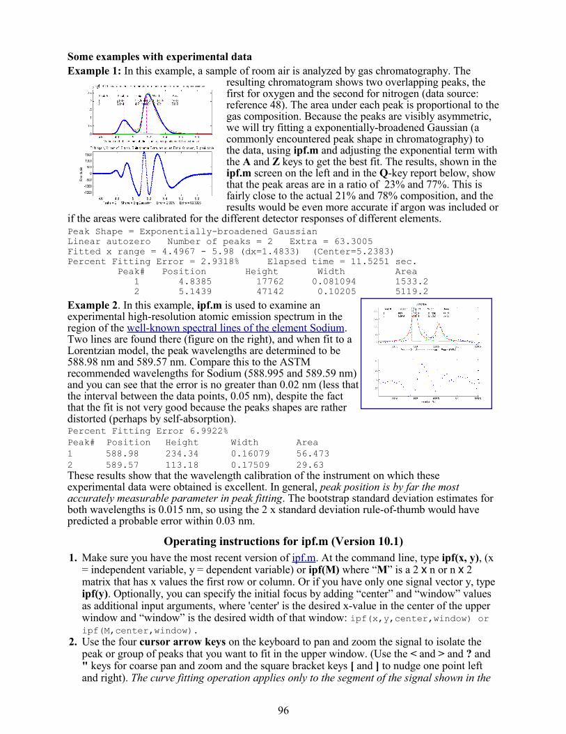
Some examples with experimental dataExample 1: In this example, a sample of room air is analyzed by gas chromatography. The

resulting chromatogram shows two overlapping peaks, the first for oxygen and the second for nitrogen (data source: reference 48). The area under each peak is proportional to the gas composition. Because the peaks are visibly asymmetric, we will try fitting a exponentially-broadened Gaussian (a commonly encountered peak shape in chromatography) to the data, using ipf.m and adjusting the exponential term with the A and Z keys to get the best fit. The results, shown in the ipf.m screen on the left and in the Q-key report below, show that the peak areas are in a ratio of 23% and 77%. This is fairly close to the actual 21% and 78% composition, and the results would be even more accurate if argon was included or

if the areas were calibrated for the different detector responses of different elements.Peak Shape = Exponentially-broadened GaussianLinear autozero Number of peaks = 2 Extra = 63.3005Fitted x range = 4.4967 - 5.98 (dx=1.4833) (Center=5.2383) Percent Fitting Error = 2.9318% Elapsed time = 11.5251 sec. Peak# Position Height Width Area 1 4.8385 17762 0.081094 1533.2 2 5.1439 47142 0.10205 5119.2

Example 2. In this example, ipf.m is used to examine an experimental high-resolution atomic emission spectrum in the region of the well-known spectral lines of the element Sodium. Two lines are found there (figure on the right), and when fit to a Lorentzian model, the peak wavelengths are determined to be 588.98 nm and 589.57 nm. Compare this to the ASTM recommended wavelengths for Sodium (588.995 and 589.59 nm) and you can see that the error is no greater than 0.02 nm (less that the interval between the data points, 0.05 nm), despite the fact that the fit is not very good because the peaks shapes are rather distorted (perhaps by self-absorption). Percent Fitting Error 6.9922%Peak# Position Height Width Area1 588.98 234.34 0.16079 56.4732 589.57 113.18 0.17509 29.63These results show that the wavelength calibration of the instrument on which these experimental data were obtained is excellent. In general, peak position is by far the most accurately measurable parameter in peak fitting. The bootstrap standard deviation estimates for both wavelengths is 0.015 nm, so using the 2 x standard deviation rule-of-thumb would have predicted a probable error within 0.03 nm.

Operating instructions for ipf.m (Version 10.1)1. Make sure you have the most recent version of ipf.m. At the command line, type ipf(x, y), (x

= independent variable, y = dependent variable) or ipf(M) where “M” is a 2 x n or n x 2 matrix that has x values the first row or column. Or if you have only one signal vector y, type ipf(y). Optionally, you can specify the initial focus by adding “center” and “window” values as additional input arguments, where 'center' is the desired x-value in the center of the upper window and “window” is the desired width of that window: ipf(x,y,center,window) or ipf(M,center,window).

2. Use the four cursor arrow keys on the keyboard to pan and zoom the signal to isolate the peak or group of peaks that you want to fit in the upper window. (Use the < and > and ? and " keys for coarse pan and zoom and the square bracket keys [ and ] to nudge one point left and right). The curve fitting operation applies only to the segment of the signal shown in the

96

top plot. The bottom plot shows the entire signal. Try not to get any undesired peaks in the upper window or the program may try to fit them.

3. Press the number keys (1– 9) to choose the number of model peaks, that is, the minimum number of peaks that you think will suffice to fit this segment of the signal. For more than 9 peaks, press 0 , type the number of peaks, and press Enter.

4. Select the desired model peak shape by pressing the '-' key and selecting the desired shape by number from the menu that is displayed. Or you can also type in a vector of shape numbers with a different shape for each peak, e.g. [1 2 1]. Or you can select single-shape models directly by pressing the following keys: Gaussian (lower case g), equal-width Gaussians (lower case h), fixed-width Gaussians (Shift-G), fixed-position Gaussians (Shift-P), exponentially-broadened Gaussian (e), exponentially-broadened equal-width Gaussians (j); bifurcated Gaussian (Shift-H), Lorentzian (lower case L), exponentially-broadened Lorentzian (Shift-E); fixed-width Lorentzians (Shift-L), fixed-position Lorentzians (Shift [ ), equal-width Lorentzians (lower case ;), bifurcated Lorentzian (:), Voigt (Shift-V) , logistic (lower case o), Pearson (lower case p), exponential pulse (u); alpha function (Shift-U) sigmoid (s); and Gaussian/Lorentzian blend (`). If the peak widths of each group of peaks is expected to be the same or nearly so, select the Equal- width or fixed-width fits (available only for the Gaussian and Lorentzian shapes), which are faster, easier, and much more stable than regular variable-width fits, especially if the number of model peaks is greater than 3 (because there are fewer variable parameters for the program to adjust).

5. A set of vertical dashed lines are shown on the plot, one for each model peak. Try to fine-tune the Pan and Zoom keys so that the signal drops down to the baseline at both ends of the upper plot and so that the peaks (or bumps) in the signal roughly line up with the vertical dashed lines. This does not have to be exact.

6. If you want to allow negative peaks as well as positive peaks, press the + key to flip to the +/- mode (indicated by the +/- sign in the y-axis label of the upper panel). Press it again to return to the + mode (positive peaks only). You can switch at any time.

7. Press F to initiate the curve-fitting calculation. Each time press F, another fit of the selected model to the data is performed with slightly different starting positions, so that you can judge the stability of the fit with respect to starting guesses. (To judge the stability of the fit with respect to noise in the data, press N. See #16). Keep your eye on the residuals plot and on the “Error” display. Do this several times, trying for the lowest error and the most unstructured random residuals plot. If the fit is unstable, try pressing X, which takes longer to compute but may give better results. At any time, you can refine the signal region to be fit (step 2), change the number or peaks (step 3), peak shape (step 4), or change the baseline correction mode (T key) to get a better fit.

8. The model parameters of the last fit are shown the upper window. For a 3-peak fit:Peak# Position Height Width Area 1 5.33329 14.8274 0.262253 4.13361 2 5.80253 26.825 0.326065 9.31117 3 6.27707 22.1461 0.249248 5.87425

The column are, left to right: the peak number, peak position, peak height, peak width, and the peak area. Press R to print this table out in the command window. Peaks are numbered from left to right. (The area of each component peak within the upper window is computed using the trapezoidal method). Pressing Q prints out a report of settings and results in the command window, like so:Peak Shape = GaussianPositive peaks onlyFlat baseline modeNumber of peaks = 3Fitted range = 5 - 6.64Percent Error = 7.4514Peak# Position Height Width Area1 5.33329 14.8274 0.262253 4.13361

97

2 5.80253 26.825 0.326065 9.311173 6.27707 22.1461 0.249248 5.87425

9. To select the baseline correction mode, press the T key repeatedly; it cycles thorough None, linear, quadratic, and flat. In linear mode, a straight-line baseline connecting the two ends of the signal segment in the upper panel will be automatically subtracted. In quadratic mode, a parabolic baseline connecting the two ends of the signal segment in the upper panel will be automatically subtracted. (Use quadratic mode if the baseline is curved). Use the flat mode if the signal does not return to the baseline at the ends.

10. If you prefer to set the baseline manually, press the B key, then click on the baseline to the LEFT of the peak(s), then click on the baseline to the RIGHT of the peak(s). The new baseline will be subtracted and the fit re-calculated. (The new baseline remains in effect until you use the pan or zoom controls). Alternatively, you may use the multi-point background correction for the entire signal: press the Backspace key, type in the desired number of background points and press the Enter key, then click on the baseline starting at the left of the lowest x-value and ending to the right of the highest x-value. Press \ to restore the previous background to start over.

11. If the peaks are not approximately lined up with the dotted magenta marker lines, it may help to manually customize the first-guess peak positions: press C, then click on your estimates of the peak positions in the upper graph, once for each peak. The fit is automatically performed after the last click. Peaks are numbered in the order clicked. Or type Shift-C to type or paste in the start vector, e.g. “[pos1 wid1 pos2 wid2 ...]”. (The custom start values remain in effect until you change the number of peaks or use the pan or zoom controls).

12. The A and Z keys control the “extra” parameter that is used only if you are using Pearson, exponentially-broadened Gaussian and Lorentzian (ExpGaussian and ExpLorentzian), bifurcated Gaussian or Lorentzian, Gaussian/Lorentzian blend, or Voigt models. For the Pearson shape, an “extra” value of 1.0 gives a Lorentzian shape, a value of 2.0 gives a shape roughly half-way between a Lorentzian and a Gaussian, and a larger values give a nearly Gaussian shape. For the exponentially broadened Gaussian shapes, “extra” controls the exponential “time constant” (expressed as the number of points). For the Gaussian/Lorentzian blend and the bifurcated Gaussian and Lorentzian shapes, “extra” controls the peak asymmetry (a values of 50 gives a symmetrical peak). You can also enter an initial value of “extra” directly by pressing Shift-X , typing in a value (or vector, for multiple shape models), and pressing the Enter key. Then you can adjust this value using the A and Z keys (hold down the Shift key to fine tune). Seek to minimize the Error % or set it to a previously-determined value. (Note: if fitting multiple overlapping peaks with an “extra” parameter, it's easier to fit a single peak first, to get a rough value for the “extra” parameter, then just fine-tune that parameter for the multi-peak fit if necessary).

13. For difficult fits, press X, which performs ten silent trial fits with slightly different first guesses and takes the one with positive peaks heights and the lowest fitting error. This also resets the starting points for subsequent fits, so pressing X repeatedly will usually converge on the best fit. (You can change the number of trials,”NumTrials”, in or near line 222 in ipf.m; the default is 10). Remember: equal-width Gaussian (H key) and Lorentzian (; key) shapes, and exponentially-broadened equal-width Gaussian (J key) peak shapes and fixed-width Gaussian (Shift-G key) shapes Lorentzian (Shift-L key) shapes, are both faster, easier, and much more stable than regular variable-width fits, so use equal-width fits whenever the peak widths are expected to be equal or nearly so, or fixed-width fits when the peak widths are known.

14. Press Y to display the entire signal full screen without cursors, with the last fit displayed in green. The residual is displayed in red, on the same y-axis scale.

15. Press M to switch the Y-axis of the full-signal plot in the bottom window between log and linear scales. This does not effect the fit, only the full-signal plot. It's useful for inspecting the signal if the amplitude range is very large.

98

16. Press the D key to print out a table of model data in the command window (x, y1, y2, ..., where x is the column of x values of the fitted region and the y's are the y-values of each component, one for each peak in the model. You can then Copy and Paste this table into a spreadsheet or data plotting program of your choice.

17. Press W to print out the ipf.m function in the command window with the current values of 'center' and 'window' as input arguments. This is useful when you want to return to that specific data segment later. Also prints out peakfit.m with all input arguments, including the last best-fit values of the first guess vector. You can copy and Paste the peakfit.m function into your own code.

18. ipf.m versions 8.12 and above can estimate the expected variability of the peak position, height, width, and area from the signal, by using the bootstrap sampling method (see page 41 - 42). This involves extracting 100 bootstrap samples from the signal, fitting each of those samples with the model, then computing the percent relative standard deviation (RSD) and the interquartile range (IQR) of the parameters of each peak. Basically this method calculates weighted fits to a single data set, using a different set of different weights for each fit. (The process is computationally intensive can take several minutes to complete, especially if the number of peaks in the model is high or if you are using an exponentially broadened shape). To activate this process, press the V key. It first asks you to type in the number of “best-of-x” trial fits per bootstrap sample (the default is 1, but you may will need a higher number here if the fits are too unstable). The results are displayed in the command window. For example, for a three-peak fit (to the same three peaks used by the Demoipf demonstration script described in the next section):

>> Number of fit trials per bootstrap sample (0 to cancel): 10

Computing bootstrap sampling statistics....May take several minutes. Peak #1 Position Height Width Area Bootstrap Mean: 800.5387 2.969539 31.0374 98.10405 Bootstrap STD: 0.20336 0.02848 0.5061 1.2732 Bootstrap IQR: 0.21933 0.027387 0.5218 1.1555 Percent RSD: 0.025402 0.95908 1.6309 1.2978 Percent IQR: 0.027398 0.92226 1.6812 1.1778 Peak #2 Position Height Width Area Bootstrap Mean: 850.0491 1.961368 36.4809 75.98684 Bootstrap STD: 6.4458 0.14622 3.0657 4.7596 Bootstrap IQR: 0.52358 0.058845 1.4303 3.9161 Percent RSD: 0.75828 7.4549 8.4035 6.2637 Percent IQR: 0.061594 3.0002 3.9205 5.1537 (Peak #3, etc.....) Elapsed time is 98.394381 seconds. Min/Max Fitting Error of the 100 bootstrap samples: 3.0971/2.5747

Observe that the percent RSD and IRQ of the peak positions are lowest, followed by heights and widths and areas. This is a typical pattern. Also, remember that these results depend on the assumption that the noise in the signal is unsmoothed and is representative of the average noise in repeated measurements. If the number of data points in the signal is small, these estimates can be very approximate. Don't smooth the data beforehand; that will cause the bootstrap to underestimate the variability drastically.

One pitfall with the bootstrap method when applied to iterative fits is the possibility that one (or more) of the bootstrap fits will go astray, that is, will result in peak parameters that are wildly different from the norm, causing the estimated variability of the para-meters to be too high. For that reason, in ipf 8.7, the interquartile range (IQR) as well as the standard deviation (STD) is reported. The IQR is more robust to outliers. For a normal distribution, the interquartile range is equal to 1.34896 times the standard deviation. But if one or more of the bootstrap sample fits fails, resulting in a distribution of peak parameters with large outliers, the STD will be much greater than the IQR. In that case, a more realistic estimate of standard deviation without the outliers is IRQ/1.34896.

99

It's best to try to increase the fit stability by choosing a better model (for example, using an equal-width of fixed-width model, if appropriate), adjusting the fitted range (pan and zoom keys), the background subtraction (T or B keys), or the start positions (C key), and/or selecting a higher number of fit trials per bootstrap (which will increase the computation time). As a quick preliminary test of bootstrap fit stability, the N key will perform a single fit to a single random bootstrap sample and plot the result; do that several times to see whether the bootstrap fits are stable enough to be worth computing the statistics of 100 bootstrap samples. Note: it's normal for the stability of the bootstrap sample fits (N key) to be poorer than the full-sample fits (F key) because the latter includes only the variability caused by changing the starting positions for one set of data and noise, whereas the N and V keys aim to include the variability caused by the random noise in the sample by fitting bootstrap sub-samples. Moreover, the best estimates of the measured peak parameters are those obtained by the normal fits of the full signal (F and X keys), not the means reported for the bootstrap samples (V and N keys), because there are more independent data points in the full fits and because the bootstrap means are influenced by the outliers that occur more commonly in the bootstrap fits. Use the bootstrap results for estimating the variability of the peak parameters, not for estimating their mean values.

Demo ipf.m Demo ipf.m is a demonstration script for ipf.m, with a built-in simulated signal generator. The true values of the simulated peak positions, heights, and widths are displayed in the Matlab command window, for comparison to the Fit Results obtained by peak fitting. The default simulated signal contains six independent groups of peaks that you can use for practice: a triplet near x = 150, a singlet at 400, a doublet near 600, a triplet near 850, and two broad single peaks at 1200 and 1700. Run this demo and see how close to the actual true peak parameters you can get. The useful thing about a simulation like this is that you can get a feel for the accuracy of peak parameter measurements, that is, the difference between the true and measured values of peak parameters. To run it it, place both ipf.m and Demo ipf in the Matlab path, then type Demoipf at the Matlab command prompt. A ZIP file containing peakfit.m, DemoPeakFit.m, ipf.m, Demoipf.m, and some data for testing is available at from http://terpconnect.umd.edu/~toh/spectrum/ipf10.zip .

An example of the use of this script is shown above. Here we focus in on the 3 fused peaks located near x=850. The true peak parameters (before the addition of the noise) are: Position Height Width Area 800 3 30 95.808 850 2 40 85.163 900 1 50 53.227

When these peaks are isolated in the upper window and fit with three Gaussians, the typical measured peak parameters are: Position Height Width Area 800.04 3.0628 29.315 95.583 850.15 1.9881 41.014 86.804 901.3 0.9699 46.861 48.376

So you can see that the accuracy of the measurements are excellent for peak position, good for peak height, and least good for peak width and area. The least accurate measurements are for the smallest peak with the poorest signal-to-noise ratio. Note: The expected standard deviations of these peak parameters can be determined by the bootstrap sampling method (page 41 - 42), as described in the previous section. We would expect that the measured values of the peak parameters (comparing the true to the measured values) would be within about 2 standard deviations of the true values listed above).

100

In this example with experimental data, pan and zoom controls are used to isolate a segment of a chromatogram that contains three very weak peaks near 5.8 minutes The lower plot shows the whole chromatogram and the upper

plot shows the segment. Only the peaks in that segment are subjected to the fit. Pan and zoom are adjusted so that the

signal returns to the local baseline at the ends of the segment.

Pressing T sets the baseline mode to linear, causing the program to compute and subtract a linear baseline between the ends of the upper segment. Pressing 3, E, F performs a

3-peak exponentially-broadened Gaussian fit. The time constant of the exponential is adjusted by the A and Z keys.

The randomness and lack of obvious structure of the residuals indicates that the fit is as good as possible with

this level of noise.

Execution timeBy “execution time” I mean the time it takes for one fit to be performed, exclusive of plotting or printing the results. The major factors that determine the execution time are the peak shape, the number of peaks, and the speed of the computer:

a) The execution time varies greatly (sometimes by a factor of 100 or more) with the peak shape, with the exponentially-broadened Gaussian being the slowest and the fixed-width Gaussian being the fastest. See Peakfit TimeTest2.m and Peakfit TimeTest2a.m. The equal-width and fixed-width shape variations are always faster than the corresponding variable-width models.

b) The execution time typically increases with the square of the number of peaks in the model.

c) The execution time can vary over a factor of 4 or 5 or more between different computers, for example, between a small laptop with 1.6 GHz, dual core Athlon CPU and 4 Gbytes RAM, compared to a big desktop with a 3.4 GHz i7 CPU and 16 Gbytes RAM). Run the Matlab “bench.m” benchmark test to see how your computer stacks up compared to other computers.

d) The execution time increases directly with NumTrials in peakfit.m; the “Best of 10 trials” function (X key in ipf.m) takes about 10 times longer than a single fit.

e) Other factors that influence execution time but are less important are (1) the number of data points in the fitted region (see Peakfit TimeTest3.m) and (2) the starting values (good starting values can reduce execution time slightly; Peakfit TimeTest2.m and Peakfit TimeTest2a.m have examples. (Some of these scripts need Data Matrix2.mat and Data Matrix3.mat).

Note 1: Matlab and Octave have “tic” and “toc” functions that are useful for determining execution time of your code. Note that the ipf.m version 8.92 and above displays the elapsed time to the reports printed by the Q and R keys. Note 2: All these scripts (m-files) and data files (mat-files) can be downloaded from http://tinyurl.com/cey8rwh.

101

ipf 10.1 Keyboard Controls Pan signal left and right...Coarse: < and > Fine: left and right cursor arrow keys Nudge: [ ] Zoom in and out.............Coarse zoom: / and " Fine zoom: up and down cursor arrow keys Resets pan and zoom.........ESC Select # of peaks...........Number keys 1-9, or press 0 key to enter manually Select peak shape from menu - (minus or hyphen), type number or vector*, Enter Select peak shape by key....g Gaussian h equal-width Gaussians G (Shift-G) fixed-width Gaussians P (Shift P) fixed-position Gaussians H (Shift-H) bifurcated Gaussians (a,z keys adjust) e Exponential-broadened Gaussian j exponential-broadened equal-width Gaussians (a,z keys adjust broadening) l Lorentzian E (Shift-e) Exponential-broadened Lorentzian ; equal-width Lorentzians Shift [ fixed-position Lorentzians : bifurcated Lorentzians (a,z keys adjust shape) L (Shift-L) Fixed-width Lorentzians o LOgistic p Pearson (a,z keys adjust shape) u pUlse y=exp(-tau1.*x).*(1-exp(-tau2.*x)) U Alpha y=(x-spoint)./pos.*exp(1-(x-spoint)./pos) s Sigmoid: y=1/2 + 1/2*erf((x-t1)/sqrt(2*t2)) ~ Gauss/Lorentz blend (a/z keys adjust shape) V (Shift-V) Voigt profile (a/z adjusts shape) Fit.........................f Perform a single fit of the selected region. + or +/- peak mode..........+ Flips between + peaks only and +/- peak mode Cycle baseline mode.........t Cycles baseline correction (“autozero” mode) Toggle log y mode OFF/ON....m Plot linear or log Y axis on lower graph 2-point Baseline............b, then click left and right baseline Background subtraction......Backspace, then click baseline at multiple points Restore original baseline...\ to cancel previous background subtraction Cursor start positions......c, then click on each peak position Type in start vector........C (Shift-C) Type or Paste [pos1 wid1 pos2 wid2 ...] Enter value of 'Extra'......Shift-x, type value or vector*, press Enter. Adjust 'Extra' up/down......a,z: 5% change. Upper case A,Z: 0.5% change**. Print parameters & results..q Print fit results only......r Compute bootstrap stats.....v Estimates standard deViations of parameters. Fit single bootstrap........n Extracts and Fits siNgle bootstrap sub-sample. Plot signal in figure 2.....y Print model data table......d Refine fit..................x Takes best of 10 trial fits (change in line 177) Print ipf and peakfit ......w Print ipf and peakfit with all input arguments Display current settings....Shift-? displays table of current values

* To specify a multiple shape model, press '-', type a vector of "Shape" values, one for every peak, enclosed in square brackets, e.g. [1 1 3], and press Enter.** The A and Z keys adjust the “extra” variable that controls the alpha of the Voigt profile, the time constant of the exponentially broadened Gaussian and Lorentzian, the peak shape of the Pearson, bifurcated Gaussian and Lorentzian, and the % Gaussian character of the Gaussian-Lorentzian blend. Notes concerning ipeak.m, isignal.m, and ipf.m: (a) Make sure you don't click on the “Show Plot Tools” button in the toolbar above the figure; that will disable normal program functioning. If you do; close the Figure window and start again. (b) To make it easier for you to transfer settings from one of these functions to another or to a command-line version, all these functions use the W key to print out the syntax of other related functions, with the pan and zoom settings and other numerical input arguments specified, ready for you to Copy, Paste and edit into your own scripts or back into the command window. For example, you can convert a curve fitting operation performed in ipf.m into the command-line peakfit.m function; or you can convert a peak finding operation performed in ipeak.m into a command-line findpeaks.m or findpeaksb.m or findpeaksb3.m functions.

102

6. Hyperlinear analytical absorption spectroscopyThis is a Matlab implementation of a computational method for quantitative analysis by multi-wavelength absorption spectroscopy, called the transmission-fitting or “TFit” method, based on fitting a model of the instrumentally-broadened transmission spectrum to the observed transmission data, rather than the conventional calculation of absorbance as log10(Izero/I). The method is described in References 25, 26, and 27 on page 116. It is included here because it combines several important concepts that are covered in this essay: signal-to-noise ratio (page 6), Fourier convolution (page 31), multicomponent spectroscopy (page 49), iterative least-squares fitting (page 54), and calibration (page 47).

Advantages of the TFit method compared to conventional absorbance-based methods are:

(a) much wider dynamic range;

(b) greatly improved calibration linearity;

(c) ability to operate under conditions that are optimized for signal-to-noise ratio rather than for absorbance linearity (e.g. small spectrometers with low dispersion and large slit widths).

Just like the multilinear regression (classical least squares) methods conventionally used in absorption spectroscopy (Page 49), the Tfit method (a) requires an accurate reference spectrum of each analyte, (b) utilizes multi-wavelength data such as would be acquired on diode-array, Fourier transform, or automated scanning spectrometers, and (c) applies both to single-component and multi-component mixture analysis.

The disadvantages of the TFit method are:

(a) it is computationally more intensive than the multilinear regression methods (but, on a typical personal computer, calculations take only a fraction of a second, even for the analysis of a mixture of three components);

(b) it requires knowledge of the instrument function, i.e., the slit function or the resolution function of an optical spectrometer (however, this is a fixed characteristic of the instrument and is easily measured beforehand by scanning the spectrum of a narrow atomic line source such as a hollow cathode lamp); and

(c) it is an iterative method that can under unfavorable circumstances converge on a local optimum (but this is handled by proper selection of the starting values, based on preliminary approximations calculated by conventional methods). If you are viewing this on-line, click here to download a self-contained demo m-file that works in recent versions of Matlab. (You can also download the ZIP file “ TFit.zip” that contains both the newer version and the older one for Matlab 6.5) and you can also download it from the Matlab File Exchange.

BackgroundIn a bsorption spectroscopy, the intensity I of light passing through an absorbing sample is given (in Matlab/Octave notation) by the Beer-Lambert Law:

I = Izero.*10^-(alpha*L*c)where “Izero” is the intensity of the light incident on the sample, “alpha” is the absorption coefficient of the absorber, “L” is the distance that the light travels through the material (the path length), and “c” is the concentration of absorber in the sample. The variables I, Izero, and alpha are all functions of wavelength; L and c are scalar.

In conventional applications, measured values of I and Izero are used to compute the quantity called “absorbance”, defined as

A = log10(Izero./I)

103

Absorbance is defined in this way so that, when you combine this definition with the Beer-Lambert law, you get:

A = alpha*L*c

So, absorbance is proportional to concentration, ideally, which simplifies analytical calibration. However, any real spectrometer has a finite spectral resolution, meaning that the light beam passing through the sample is not truly monochromatic, with the result that an intensity reading at one wavelength setting is actually an average over a small spectral interval. More exactly, what is actually measured is the convolution of the true spectrum of the absorber and the instrument function. If the absorption coefficient “alpha” varies over that interval, then the calculated absorbance will no longer be linearly proportional to concentration (this is called the “polychromicity” error). The effect is most noticeable at high absorbances. In practice, many instruments will become non-linear starting at an absorbance of 2 (~1% Transmission). As the absorbance increases, the effect of unabsorbed stray light and instrument noise also becomes more significant. Traditionally, there was no way to circumvent these problems, and the non-linearity so produced made calibration more complex and less certain.

The theoretical best signal-to-noise ratio and absorbance precision for a photon-noise limited optical absorption instrument can be shown to be close to an absorbance of 1.0 (see http://terpconnect.umd.edu/~toh/models/AbsSlitWidth.html#Best Absorbance). However, if one attempts to arrange sample dilutions and absorption cell path lengths to obtain a working range centered on an absorbance of 1.0 , for example over the range .1 – 10, or 0.01 – 100, the measurements will obviously fail at the high end. (Clearly, the direct measurement of an absorbance of 100 is unthinkable, as it implies the measurement of light attenuation of 100 powers of ten - no real measurement system has a dynamic range remotely close to that). In practice, it is difficult to achieve an dynamic range even as high as 5 or 6 absorbance, so that much of the theoretically optimum absorbance range is actually unusable. (c.f. http://en.wikipedia.org/wiki/ Absorbance). So, in conventional practice, greater sample dilutions and shorter path lengths are required to force the absorbance range to lower values, even if this means poorer signal-to-noise ratio and measurement precision at the low end.

It is true that the non-linearity caused by polychromicity can be reduced by operating the instrument at the highest resolution setting (reducing the instrumental slit width). However, this has a serious undesired side effect: in dispersive instruments, reducing the slit width to increase the spectral resolution degrades the signal-to-noise substantially. The optimum signal-to-noise ratio is often achieved when the resolution of the instrument approximately matches the width of the analyte absorption, but operating the instrument in that way would result in very substantial non-linearity over most of the absorbance range because of the “polychromicity” error.

The Fit method sidesteps the above problems by calculating the absorbance in a completely different way: it starts with the reference spectra (an accurate absorption spectrum for each analyte, recorded in the linear absorbance range, which is also required by the multilinear regression methods described on page 49), normalizes them to unit height, multiplies each by an adjustable coefficient (usually equal to the conventional absorbance measurement for that component in the mixture), adds them up, computes the transmission spectrum by taking the antilog, and convolutes it (page 31) with the previously-measured slit function. The result, representing the instrumentally broadened transmission spectrum, is compared to the observed transmission spectrum. The adjustable coefficients (one for each unknown component in the mixture) are adjusted by Simplex Optimization (page 54) until the computed transmission model is a least-squares best fit to the observed transmission spectrum. The best-fit coefficients are then equal to the absorbances that would have been observed under ideal optical conditions. Provision is also made to compensate for unabsorbed stray light and changes in background

104

intensity (background absorption). The Fit method gives measurements of absorbance that are much closer to the “true” peak absorbance that would have been measured in the absence of stray light and polychromatic light errors, and it allows linear and wide dynamic range measurements to be made even if the slit width of the instrument is increased to optimize the signal-to-noise ratio. (The calculations are performed by the function fitM, which is used as a fitting function for the iterative non-linear fitting function fminsearch.m in Matlab or Octave).

The TFit method does not guarantee a perfectly linear analytical curve under all conditions, despite the impression given by these simulations. It simply removes the non-linearity caused by unabsorbed stray light and the polychromatic light effect. Other sources of non-linearity remain - in particular, chemical effects such as photolysis, equilibrium shifts, temperature effects, pH effects, binding, dimerization, polymerization, molecular phototropism, fluorescence, etc.

Note: It's important to understand that the TFit method is based on the Beer-Lambert Law, but it just calculates the absorbance in a different way that does not require the assumption that stray light and polychromatic radiation effects are zero. Because it allows larger slit widths to be used, it is possible to obtain greater signal-to-noise ratios, while still achieving a much wider linear dynamic range than usual.

The fitM.m function

function err = fitM(lam,yobsd,Spectra,InstFun,StrayLight)

fitM is a fitting function for the Tfit method, for use with the fminsearch function (page 55). The input arguments of fitM are:

lam = vector of adjustable parameters (in this case, peak absorbances) that are varied to obtained the best fit.yobsd = observed transmission spectrum of the mixture sample over the spectral range (column vector)Spectra = reference spectra for each component, over the same spectral range, one column/component, normalized to 1.00. InstFun = Zero-centered instrument function or slit function (column vector)StrayLight = fractional stray light (scalar or column vector, if it varies with wavelength)

Note: yobsd, Spectra, and InstFun must have the same number of rows (wavelengths). Spectra must have one column for each absorbing component.

Typical use: absorbance=fminsearch(@(lambda)(fitM(lambda, yobsd, TrueSpectrum, InstFunction, straylight)), start);

where start is the first guess (or guesses) of the absorbance(s) of the analyte(s); it's convenient to use the conventional log10(Izero/I) estimate of absorbance(s) for start. The other arguments (described above) are passed on to FitM. In this example, fminsearch returns the value of absorbance that would have been measured in the absence of stray light and polychromatic light errors (which is either a single value or a vector of absorbances, if it is a multicomponent analysis). The absorbance can then be converted into concentration by any of the usual calibration procedures (Beer's Law, external standards, standard addition, etc.)

Iterative least-squares methods (page 54) are ordinarily considered to be more difficult and less reliable than multilinear regression methods (page 49), and this can be true if there are more than one nonlinear variable that must be iterated, especially if those variables are correlated. However, in the TFit method, there is only one iterated variable (absorbance) per measured component, and reasonable first guesses are easily available from the conventional single-wavelength absorbance calculation or multiwavelength regression methods. As a result, an

105

iterative least-squares method works very well in this case. Comparing the expression for absorbance given above for the TFit method to that for the weighted regression method:

absorbance=([weight weight].*[Background ReferenceSpectra])\(-log10(yobsd).*weight)

You can see that, in addition to the ReferenceSpectra and observed transmission spectrum (yobsd), the TFit method also requires a measurement of the Instrument function (spectral bandpass) and the stray light (which the linear regression methods assume to be zero), but these are characteristics of the spectrometer and need be done only once for a given spectrometer. Finally, although the TFit method does make the computer work harder, the computation time on a typical laboratory personal computer is only a fraction of a second (roughly 25 µsec per spectral data point per component analyzed), using Matlab as the computational environment.

Basic demo of the Tfit method: TfitDemo.m (Matlab) and tfit.m (Octave)

The Matlab-only script TfitDemo is an interactive explorer for the Tfit method applied to the measurement of a single component with a Lorentzian or Gaussian absorption peak, with keystroke controls for adjusting the parameters while observing the effects graphically and numerically. The adjustable parameters are: the true absorbance, “True A” (adjusted with the A/Z keys), the spectral width of the absorption peak, “AbsWidth”, (adjusted with the S/X keys), the spectral width of the slit function, “SlitWidth” (adjusted with the D/C keys), the percent stray light, “Straylight” (adjusted with the F/V keys), and the noise level, “Noise” (adjusted with the G/B keys). (The wavelength scale, and the values of both AbsWidth and SlitWidth, are in arbitrary units).

The equivalent function for Octave users is tfit.m; the true absorbance is specified in the single input argument of that function, while the other parameters are set in lines 28-33.

The simulation includes the effect of photon noise, unabsorbed stray light, and random background intensity shifts (light source flicker), and it compares observed absorbances computed by the single-wavelength, “Single”, weighted multilinear regression, “WReg” (sometimes called Classical Least Squares in the chemometrics literature), and the TFit methods. If you are viewing this on-line, right-click TFitDemo.m click “Save link as...”, save it in a folder in the Matlab path, then type “TFitDemo” at the Matlab command prompt. With the figure window topmost, press K to get a list of the keypress functions. In the example shown in the figure above, the true peak absorbance is exactly 1.000, the absorption widths and slit function widths are equal, the unabsorbed stray light is 0.5%., and the photon noise is 5%. The results below the graphs show that the TFit method gives a much more accurate measurement (1.0056) than the single-wavelength method (0.6246) or weighted multilinear regression method (0.8883).

106

TFitDemo KEYBOARD COMMANDSPeak shape....Q.....Toggles between Gaussian and Lorentzian shapesTrue peak A...A/Z...True absorbance of analyte at peak center, without instrumental broadening, stray light, or noise.AbsWidth......S/X...Width of absorption peakSlitWidth.....D/C...Width of instrument function (spectral bandpass)Straylight....F/V...Fractional unabsorbed stray light.Noise.........G/B...Random noise levelRe-measure....Spacebar Re-measure signalSwitch mode...W.....Switch between transmission and absorbance displayStatistics....Tab...Prints table of statistics of 50 repeatsCal. Curve....M.....Displays analytical calibration curve in Figure 2Keys..........K.....Print this list of keyboard commands

Why does the noise on the graph change if I change the instrument function (slit width or InstWidth)? In the most common type of absorption spectrometer, the spectrometer's spectral bandwidth (InstWidth) is changed by changing the slit width, which also effects the light intensity and thus the signal-to-noise ratio. Therefore, in all these programs, when you change InstWidth, the photon noise is automatically changed accordingly just as it would in a real spectrophotometer.

TFitStats.m: Statistics of methods compared (Matlab or Octave)The Matlab/Octave script TFitStats computes the statistics of the TFit method compared to single- wavelength (SingleW), simple regression (SimpleR), and weighted regression (WeightR) methods. Simulates photon noise, unabsorbed stray light and random background intensity shifts. Estimates the precision and accuracy of the four methods by repeating the calculations 50 times with different random noise samples. Computes the mean, relative percent standard deviation, and relative percent deviation from true absorbance. Parameters are easily changed in lines 19 - 26. Results are displayed in the MATLAB command window. Note: This statistics function is included as a keypress command (Tab key) in the Matlab interactive demo TFitDemo.m. In the typical results shown below (for a simulation with AbsWidth=10; SlitWidth=20; Straylight=0.5%, and Noise=5% of Izero) results for true absorbances of 0.001. 1.00, and 100 are compared, demonstrating that the accuracy and the precision of these methods over a 10,000-fold concentration range.

True A SingleW SimpleR WeightR TFit

Mean result* .0010 .0003 .00057 .00070 .00097

% RSD** 435% 275% 40% 38%

% Accuracy*** -70% -40% -30% 2.30%

Mean result* 1.0000 0.599 0.656 0.841 1.001

% RSD** 0.69% 0.33% 0.27% 0.32%

% Accuracy*** -40% -34% -16% 0.07%

Mean result* 100 2.0038 3.7013 57.1530 99.9967

% RSD** 22.00% 23.00% 78.00% 6.80%

% Accuracy*** -98.00% -96.00% -43.00% 0.33%* Average value of the 50 measured absorbances** Percent relative standard deviation of the 50 measured absorbances*** Percent difference between the average of the 50 measured absorbances and the true absorbance

107

TFitCalDemo.m: Comparison of analytical curves (Matlab or Octave)

Matlab/Octave function that compares the analytical curves for single-wavelength, simple regression, weighted regression, and the TFit method over any specified absorbance range (specified by the vector “absorbancelist” in line 20). Simulates photon noise, unabsorbed stray light and random background intensity shifts. Plots a log-log scatter plot with each repeat measurement plotted as a separate point (so you can see the scatter of points at low absorbances). The parameters can be changed in lines 43 - 51.

In the sample result shown above, analytical curves for the four methods are computed over a 10,000-fold range, up to a peak absorbance of 100, demonstrating that the TFit method (shown by the green circles) is much more nearly linear over the whole range than the single-wavelength, simple regression, or weighted regression methods. Note: This calibration curve function is included as a keypress command (M key) in the Matlab interactive demo function TFitDemo.m.

Application to a three-component mixture: TFit3Demo.m and Tfit3.m

Tfit3Demo is a Matlab interactive demonstration function of the T-Fit method applied to the multicomponent absorption spectroscopy of a mixture of three absorbers, with keystrokes that allow you to adjust the parameters continuously while observing the effect dynamically. The adjustable parameters are: the absorbances of the three components (A1, A2, and A3, adjusted by the A/Z, S/X, and D/C keys respectively), spectral overlap between the component spectra (“Sepn”, adjusted by the F/V keys), width of the instrument function (“InstWidth” adjusted by the G/B keys), and the noise level (“Noise”, adjusted by the H/N keys). The equivalent function for Octave users is Tfit.m, which has the syntax Tfit(AbsorbanceVector), where

108

AbsorbanceVector is the vector of the three true absorbances in the mixture, e.g.: TFit3([3 .1 5]).

This demonstration compares quantitative measurement by weighted regression (page 50) and TFit methods. It simulates photon noise, unabsorbed stray light and random background intensity shifts. Note: After executing this m-file, slide the “Figure 1” and “Figure 2” windows side-by-side so that they don't overlap. Figure 1 shows a log-log scatter plot of the true vs. measured absorbances, with the three absorbers plotted in different colors and symbols. Figure 2 shows the transmission spectra of the three absorbers plotted in the corresponding colors. As you adjust the variable parameters in Figure No. 1, both graphs change accordingly.

In the sample calculation shown above, component 2 (shown in blue) is almost completely buried by the stronger absorption bands on either side, giving a much weaker absorbance (0.1) that the other two components (3 and 5, respectively). Even in this case the TFit method gives a result within 1 to 2% of the correct value (A2=0.1). In fact, over most combinations of the three concentrations, the TFit method works better, although of course nothing works if the spectral differences between the components is too small. (In this program, as in all of the above, when you change InstWidth, the photon noise is automatically changed accordingly just as it would in a real spectrophotometer).

TFitDemo3 KEYBOARD COMMANDSA1..........A/Z Increase/decrease true absorbance of component 1A2..........S/X Increase/decrease true absorbance of component 2A3..........D/C Increase/decrease true absorbance of component 3Sepn........F/V Increase/decrease spectral separation of the componentsInstWidth...G/B Increase/decrease width of spectral bandpassNoise.......H/N Increase/decrease random noise level when InstWidth = 1Peak shape..Q Toggles between Gaussian and Lorentzian absorption peak shapeTable.......Tab Print table of resultsKeys........K Print this list of keyboard commands

Another run of the same simulation, showing the sample table of results obtained by pressing the Tab key: True Weighted TFit absorbance Regression methodComponent 1 3.00 2.06 3.001 Component 2 0.10 0.4316 0.098 Component 3 5.00 2.464 4.998 Note for Octave users: the current versions of fitM.m, tfit.m, TfitStats.m and TfitCalDemo.m work in Octave as well as in Matlab. However, the interactive features of TfitDemo.m and Tfit3Demo.m work only in Matlab; Octave users should use the command-line functions tfit.m and Tfit3.m. See http://tinyurl.com/cey8rwh for a list of and links to these and other Matlab and Octave functions.

109

Appendix: More on smoothing This section presents additional supporting information related to smoothing (page 11).

A. Can smoothed noise may be mistaken for an actual signal? Here are two examples that show that the answer to this question is yes. The first example is shown on the left. This shows iSignal (page 85) displaying a computer-generated 4000-point signal consisting of pure random noise, smoothed with a 19-point Gaussian smooth. The upper window shows a tiny slice of this signal that looks like a Gaussian peak with a calculated SNR over 1000. Only by looking at the entire signal (bottom window) do you see the true picture; that “peak” is just part of the noise, smoothed to look nice. Don't fool yourself.

The second example is a simple series of three Matlab commands that uses the 'randn' function to generate a 10000-point data set containing only normally-

distributed white noise. Then it uses 'fastmooth' (page 15-16) to smooth that noise, resulting in a 'signal' with a standard deviation of about 0.3 and a maximum value around 1.0. That signal is then submitted to iPeak (page 78). If the peak detection criteria (e.g. AmpThreshold and SmoothWidth) are set too low, many peaks will be found. But setting the AmpThreshold to 3 times the standard deviation (3 x 0.3 = 0.9) will greatly reduce the incidence of these false peaks. >> noise=randn(1,10000);>> signal=fastsmooth(noise,13);>> ipeak([1:10000;signal],0,0.6,1e-006,17,17)

The peak identification function, described on page 77 and 80, which identifies peaks based on their exact x-axis peak position, is even less likely to be fooled by random noise, because in addition to the peak detection detection criteria of the findpeaks algorithm, any detected peak must also match closely to a peak position in the table of known peaks.

B. Smoothing performance comparison. The Matlab/Octave function “smoothdemo.m” (on http://tinyurl.com/cey8rwh) is a self-contained function that compares the performance of four types of smooth operations: (1) sliding-average, (2) triangular, (3) pseudo-Gaussian (equivalent

110

to three passes of a sliding-average), and (4) Savitzky-Golay. These are the four smooth types discussed on page 11, corresponding to the four values of the SmoothMode input argument of the iSignal function (page 85). These four smooth operations are applied to a 2000-point signal consisting of a Gaussian peak with a FWHM (full-width at half-maximum) of 322 points and to a noise array consisting of 107 samples of normally-distributed random white noise with a mean of zero and a standard deviation of 1.0. The peak height of the smoothed peak, the standard deviation of the smoothed noise, and the signal-to-noise ratio are all measured as a function of smooth width, for each smooth type. Smooth width is expressed in terms of “smooth ratio”, the ratio of the width of the smooth to the width (FWHM) of the peak. You may download this smooth demo function from http://tinyurl.com/cey8rwh.

The results, when “smoothdemo.m” is run (with a noise array length of 107 to insure accurate sampling of the noise), are shown by the figure and text print-out below. The four quadrants of the graph are: (upper left) the original Gaussian peak before smoothing and without noise; (upper right) the peak height of the smoothed signal as a function of smooth ratio; (lower left) the standard deviation of the noise as a function of smooth ratio; the signal-to-noise ratio (SNR) as a function of smooth ratio (lower right). The different smooth types are indicated by color: blue - sliding-average; green - triangular; red - pseudo-Gaussian, and cyan - Savitzky-Golay.

The function also calculates and prints out the elapsed time for a each smooth type and the maximum in the SNR plot.

1. Sliding-average:Elapsed Time: 0.2615; Optimum SNR: 15.1 at a smooth width of 1.26

2. Triangular:Elapsed Time: 0.5956; Optimum SNR: 15.8 at a smooth width of 1.11

3. Pseudo-Gaussian:Elapsed Time: 0.8695; Optimum SNR: 15.6 at a smooth width of 0.94

4. Savitzky-Golay:Elapsed Time: 4.4995; Optimum SNR: 20.3 at a smooth width of 1.74

These results clearly show that the Savitzky-Golay smooth gives the smallest peak distortion (smallest reduction in peak height), but, on the other hand, it gives the smallest reduction in noise amplitude and the longest computation time (by a factor of five or more). The pseudo-Gaussian smooth gives the greatest noise reduction and, below a smooth ratio of about 1.0, the highest signal-to-noise ratio, but the Savitzky-Golay smooth gives the highest SNR above a smooth ratio of 1.0.

For applications where speed is not an issue and where the shape of the signal must be preserved as much as possible, the Savitzky-Golay is clearly the method of choice. In the peak detection function described in page 74, on the other hand, the purpose of smoothing is to reduce the noise in the derivative signal and the retention of the shape of that derivative is less important. Therefore the triangular or pseudo-Gaussian smooth is well suited to this purpose and has the additional advantage of faster computation speed.

The conclusions are essentially the same for a Lorentzian peak, as demonstrated by a similar function “smoothdemoL.m”, the main difference being that the peak height reduction is greater for the Lorentzian at a given smooth ratio.

111

Case Studies A. An unusual signal.The experimental signal in this case was unusual in that it did not look like a typical signal when

plotted. In fact, at first glance it looked a lot like noise. The figure on the left compares the raw signal (bottom) with the same number of points of normally-distributed white noise (top) with a mean of zero and a standard deviation of 1.0 (obtained from the Matlab/ Octave 'randn' function). As you can see, the main difference is that the experimental signal has more large 'spikes', especially in the positive direction. This difference is evident when you look at the descriptive statistics of the signal and the randn function:

DESCRIPTIVE STATISTICS Raw signal random noise (randn function)

Mean 0.4 0

Maximum 38 about 5

Standard deviation (std) 1.05 1.0

Interquartile Range (iqr) 1.04 1.3489

Kurtosis 38 3

Skewness 1.64 0

Even though the standard deviation of these two are about the same, the other statistics (especially the kurtosis and skewness) indicate that the probability distribution of the signal is far from normal; in particular, there are far more positive spikes in the signal than expected for pure noise. Most of these are actually the peaks of interest for this signal; they look like spikes only

because the length of the signal (over 1,000,000 points) causes the peaks to be compressed into one screen pixel or less when the entire signal is plotted on the screen. In the figures on the left, iSignal (page 85) is used to “zoom in” on some of the larger of these peaks. The peaks are very sparsely separated (by an average of 1000 half-widths between peaks) and are well above the level of background noise (which has a standard deviation of roughly 0.9 throughout the signal).

The researcher who obtained this signal said that a 'good' peak was 'bell shaped', with an amplitude above 5 and a width of 500-1000 x-axis units. So that means that we can expect the signal-to-background-noise ratio to be at least 5/0.9 = 5.5. You can see in the three example peaks on the left that the peak widths do indeed meet those expectations. The interval between adjacent x-axis points is 25, so that means the we can expect the peaks to have about 20 to 40 points in their widths. Based on that, we can expect that the positions, heights and

widths of the peaks should be able to be measured fairly accurately using least-squares methods (which reduce the uncertainty of measured parameters by about the square root of the number of

112

points used, about a factor of 5 in this case). However, the noise appears to be signal-dependent (page 8); the noise on the top of the peaks is distinctly greater than the noise on the baseline. The result is that the actual signal-to-noise ratio of the peak parameter measurements for the larger peaks will not be as good as might be expected based on the ratio of the peak height to the noise on the background. Most likely, the total noise in this signal is the sum of at least two major components, one with a fixed standard deviation of 0.9 and the other equal to about 10% of the peak height.

To automate the detection of large numbers of peaks, we can use the findpeaks function (page 74). Reasonable initial values values of the input arguments AmplitudeThreshold, SlopeThreshold, SmoothWidth, and FitWidth for those functions can be estimated based on the expected peak height (5) and width (20 to 40 data points) of the “good” peaks. For example, using AmplitudeThreshold=5, SlopeThreshold=.001, SmoothWidth=25, and FitWidth=25, findpeaks detects 76 peaks above an amplitude of 5 and with an average peak width of 523.

iPeak (page 76) is especially convenient for exploring the effect of these peak detection parameters and for graphically inspecting the peaks that it finds. Ideally the objective is to find a set of peak detection arguments that detect and accurately measure all the peaks that you would consider 'good' and skip all the 'bad' ones. But in reality the criteria for good and bad peaks is at least partly subjective, so it's usually best to err on the side of caution and avoid skipping 'good' peaks at the risk of including a few 'bad' peaks, which can be weeded out manually based on unusual position, height, width, or appearance.

Of course it must be expected that the values of the peak position, height, and width given by the findpeaks or iPeak functions will only be approximate and will vary depending on the exact setting of the peak detection arguments; the noisier the data, the greater the uncertainty in the peak parameters. In this regard the peak-fitting functions peakfit.m and ipf.m (page 90, 95) may give slightly more accurate results, because they make use of all the data across the peak, not just the top of the peak as do findpeaks and iPeak. Also, the peak fitting functions are better for dealing with overlapping peaks, and they have the ability to estimate the uncertainty of the measured peak parameters, using the bootstrap options of those functions (pages 42 and 96). Using that method, the largest peak in the signal is found to have an x-axis position of 2.8683e+007, height of 32, and width of 500, with standard deviations of 4, 0.92, and 9.3, respectively.

Because the signal in the case study was so large (over 1,000,000 points), the interactive programs such as iPeak (page 74), iSignal (page 85), and ipf (page 95) may be sluggish in operation, especially if your computer is not especially fast computationally or graphically. If this is a serious problem, it may be best to break the signal up into two or more segments, deal with each segment separately, then combine the results. Alternatively, you can use the condense function to average the entire signal into a smaller number of points by a factor of 2 or 3, at the risk of slightly reducing peak heights and increasing peak widths, but then you should adjust “SmoothWidth” and “FitWidth” to compensate for the reduced number of data points across the peaks.

113

Case Studies B. Buried treasure.The experimental signal in this case, shown on the right, had a number of clearly visible narrow spikes above a seemingly flat baseline.

Using iSignal to investigate the signal, it was found that the positive spikes were single points of very large amplitude (up to 106), whereas the regions between the spikes contained bell-shaped peaks so small they can't be seen on this scale.

For example, using iSignal to zoom in to the region around x=26300, you can see one of those bell-shaped peaks, with a single-point negative spike near its peak, in the plot on the left.

Very narrow spikes like this are common artifacts in some experimental signals; they are easy to eliminate by using a median filter (page 15). iSignal has such a filter (the “M” key). The result, in

the plot on the right, shows that the single-point spike artifacts have been eliminated, with little effect on the character of the bell-shaped peak. Other filter types, like most forms of smoothing, would be far less effective than a median filter for this type of artifact and would distort the peaks. The negative spikes in this signal turned out to be negative-going steps, which can either be reduced by using iSignal's slew rate limit function (the ` key) or manually eliminated by using the

semicolon key (;) to set the selected region between the dotted red cursor lines to zero. Using the latter approach, the entire cleaned-up signal is shown on the left. The remaining peaks are all positive, smooth, bell-shaped and have amplitudes from about 6 to about 750.

iPeak can automate the estimation of peak positions, heights, and widths

for the entire signal, finding 50 peaks above the amplitude threshold (see figure on right). Individual peaks can be measured more accurately by

fitting the whole peak with iPeak's “N” key or with peakfit.m or ipf.m. The peaks are all slightly asymmetrical, fitting an exponentially-broadened Gaussian model (page 66) to a fitting error less than about 0.5%, as shown on the left. The smooth residual plots suggests that the signal was smoothed before the spikes were introduced.

114

Case Studies C. The Battle Rounds: a comparison of methods.This study simulates the application of several techniques described in this paper to the quantitative measurement of a noisy peak buried in an unstable background, a common problem in the quantitative analysis applications of various forms of spectroscopy (ref 49) and remote sensing. The object is to derive a measure of peak amplitude that varies linearly with the actual peak amplitude but that is not effected by the changes in the back-ground and the random noise. In this example, the peak to be measured is located at a fixed location in the center of the recorded signal, at x=100, and has a fixed shape (Gaussian) and width (30). The background, on the other hand, is highly variable, both in amplitude and in shape. The simulation shows six superimposed recordings of the signal with six increasing peak amplitudes and with randomly varying background amplitudes and shapes (top row left in the figures below). The signal processing techniques that are used here include smoothing (page 10), differentiation (page 16), classical least squares multicomponent method (CLS, page 48), and iterative non-linear curve fitting (page 53).

This case study is illustrated by CaseStudyC.m, a self-contained Matlab/Octave function (download from http://tinyurl.com/cey8rwh.and place in the Matlab path). To run it, just type “CaseStudyC” at the command prompt. Each time you run it, you get the same series of true peak amplitudes (set by the vector “SignalAmplitudes”) but a different set of noise, background shapes and amplitudes. The background is modeled as a Gaussian peak of randomly varying amplitude, position, and width; you can control the average amplitude of the background by changing the variable “BackgroundAmplitude” and the average change in the background by changing the variable “BackgroundChange”.

The five methods compared here are:1: Top row center. A simple zero-to-peak measurement of the smoothed signal, which will be

accurate only if the background is zero.2: Top row right. The difference between the peak signal and the average background on both

sides of the peak (both smoothed), which assumes that the background is flat.3: Bottom row left. A derivative-based method, based on the assumption that the background is

very broad compared to the measured peak.4: Bottom row center. Classical least squares (CLS, page 48), which assumes that the

background is a peak of known shape, width, and position (but not height).5: Bottom row right. iterative non-linear curve fitting (INLS, page 53), which assumes that the

background is a peak of known shape but unknown width and position. This method can track changes in the background peak position and width (within limits), as long as the measured peak and the background shapes are known.

115

These five methods are compared by plotting the actual peak heights (defined by the vector “SignalAmplitudes”) vs the measure derived from that method, fitting the data to a straight line, and computing the coefficient of determination, R2 which ideally is 1.0000.

For the first test (shown in the figure on the page 115), both “BackgroundAmplitude” and “BackgroundChange” are set to zero, so that only the random noise is present. In that case all the methods work well, with R2.values all very close to 1.0000.

For the second test (shown in the figure immediately above), the background is allowed to have significant amplitude variation but a fixed shape, position, and width, so we set “BackgroundAmplitude”=1 and “BackgroundChange”=0. In that case, the first two methods fail completely, but the derivative and INLS methods still work well.

For the third test, shown in the figure above, “BackgroundAmplitude”=1 and “BackgroundChange”=100, so the background varies in position, width, and amplitude (but remains broad compared to the signal). In that case, the CLS methods fails as well, because it assumes that the background varies only in amplitude. However, if we go one step further and set “BackgroundChange”=1000, the background shape is now so unstable that even the INLS method fails, but still the derivative method remains effective as long as the background is broader that the measured peak, whatever its shape. On the other hand, if the width and position of the measured peak changes from sample to sample, the derivative method will fail and the INLS method is more effective, as long as the basic shape of both measured peak and the background are accurately modeled.

116

References1. Douglas A. Skoog, Principles of Instrumental Analysis, Third Edition, Saunders, Philadelphia, 1984.

Pages 73-76.

2. Gary D. Christian and James E. O'Reilly, Instrumental Analysis, Second Edition, Allyn and Bacon, Boston, 1986. Pages 846-851.

3. Howard V. Malmstadt, Christie G. Enke, and Gary Horlick, Electronic Measurements for Scientists, W. A. Benjamin, Menlo Park, 1974. Pages 816-870.

4. Stephen C. Gates and Jordan Becker, Laboratory Automation using the IBM PC, Prentice Hall, Englewood Cliffs, NJ, 1989.

5. Muhammad A. Sharaf, Deborah L Illman, and Bruce R. Kowalski, Chemometrics, John Wiley and Sons, New York, 1986.

6. Peter D. Wentzell and Christopher D. Brown, Signal Processing in Analytical Chemistry, in Encyclopedia of Analytical Chemistry, R.A. Meyers (Ed.), p. 9764–9800, John Wiley & Sons Ltd, Chichester, 2000 (http://myweb.dal.ca/pdwentze/papers/c2.pdf)

7. Constantinos E. Efstathiou, Educational Applets in Analytical Chemistry, Signal Processing, and Chemometrics. (http://www.chem.uoa.gr/Applets/Applet_Index2.htm)

8. A. Felinger, Data Analysis and Signal Processing in Chromatography, Elsevier Science (1998).

9. Matthias Otto, Chemometrics: Statistics and Computer Application in Analytical Chemistry, Wiley-VCH (March 19, 1999). Some parts viewable in Google Books.

10. Steven W. Smith, The Scientist and Engineer's Guide to Digital Signal Processing. (PDF format: http://www.dspguide.com/pdfbook.htm).

11. Robert de Levie, How to use Excel in Analytical Chemistry and in General Scientific Data Analysis, Cambridge University Press; 1 edition (February 15, 2001), PDF excerpt .

12. Scott Van Bramer, Statistics for Analytical Chemistry, http://science.widener.edu/svb/stats/stats.html.

13. Numerical Analysis for Chemical Engineers, Taechul Lee (http://www.cheric.org/ippage/e/ipdata/2001/13/lecture.html)

14. Educational Matlab GUIs, Center for Signal and Image Processing (CSIP), Georgia Institute of Technology. (http://users.ece.gatech.edu/mcclella/ matlab GUIs/)

15. Digital Signal Processing Demonstrations in Matlab, Jan Allebach, Charles Bouman, and Michael Zoltowski, Purdue University (http://www.ecn.purdue.edu/VISE/ee438/demos/Demos.html)

16. Chao Yang, Zengyou He and Weichuan Yu, Comparison of public peak detection algorithms for MALDI mass spectrometry data analysis, http://www.biomedcentral.com/1471-2105/10/4

17. Michalis Vlachos, A practical Time-Series Tutorial with MATLAB, http://alumni.cs.ucr.edu/~mvlachos/PKDD05/PKDD05_Handout.pdf

18. Larry Larson, Evaluation of Calibration Curve Linearity, http://www.deq.state.va.us/waterguidance/pdf/96007.pdf.

19. Tobin A. Driscoll, A crash course in Matlab, http://www.math.umn.edu/~lerman/math5467/ matlab _adv.pdf

20. P. E. S. Wormer, Matlab for Chemists, http://www.math.ru.nl/dictaten/ Matlab / matlab _diktaat.pdf

21. Martin van Exter, Noise and Signal Processing, http://www.physics.leidenuniv.nl/sections/cm/ip/Onderwijs/SVR/bestanden/ noise -final.pdf

22. Scott Sinex, Developer's Guide to Excelets, http://academic.pgcc.edu/~ssinex/ excel ets/

23. R. de Levie, Advanced Excel for scientific data analysis, Oxford Univ. Press, N.Y. (2004)

24. S. K. Mitra, Digital Signal Processing, a computer-based approach, 4th edition, McGraw-Hill, New York, 2011.

117

25. “Calibration in Continuum-Source AA by Curve Fitting the Transmission Profile” , T. C. O'Haver and J. Kindervater, J. of Analytical Atomic Spectroscopy 1, 89 (1986)

26. “Estimation of Atomic Absorption Line Widths in Air-Acetylene Flames by Transmission Profile Modeling”, T. C. O'Haver and J-C. Chang, Spectrochim. Acta 44B, 795-809 (1989)

27. “Effect of the Source/Absorber Width Ratio on the Signal-to-Noise Ratio of Dispersive Absorption Spectrometry”, T. C. O'Haver, Anal. Chem. 68, 164-169 (1991).

28. “Derivative Luminescence Spectrometry”, Green and O'Haver, Anal. Chem. 46, 2191 (1974).

29. “Derivative Spectroscopy”, T. C. O'Haver and G. L. Green, American Lab. 7, 15 (1975).

30. “Numerical Error Analysis of Derivative Spectroscopy for the Quantitative Analysis of Mixtures”, T. C. O'Haver and G. L. Green, Anal. Chem. 48, 312 (1976).

31. “Derivative Spectroscopy: Theoretical Aspects”, T. O'Haver, Anal. Proc. 19, 22-28 (1982).

32. “Derivative and Wavelength Modulation Spectrometry,” T. C. O'Haver, Anal. Chem. 51, 91A (1979).

33. “A Microprocessor-based Signal Processing Module for Analytical Instrumentation”, T. C. O'Haver and A. Smith, American Lab. 13, 43 (1981).

34. “Introduction to Signal Processing in Analytical Chemistry”, T. C. O'Haver, J. Chem. Educ. 68 (1991)

35. “Applications of Computers and Computer Software in Teaching Analytical Chemistry”, T. C. O'Haver, Anal. Chem. 68, 521A (1991).

36. “The Object is Productivity”, T. C. O'Haver, Intelligent Instruments and Computers March-April, 1992, p 67-70.

37. Analysis software for spectroscopy and mass spectrometry, Spectrum Square Associates (http://www.spectrumsquare.com/).

38. Fityk, a program for data processing and nonlinear curve fitting. (http://fityk.nieto.pl/)39. Peak fitting in Origin (http://www.originlab.com/index.aspx?go=Products/Origin/DataAnalysis/PeakAnalysis/ PeakFit ting)

40. IGOR Pro 6, software for signal processing and peak fitting (http://www.wavemetrics.com)

41. PeakFIT, peak separation analysis (http://www.sigmaplot.com/products/ peakfit / peakfit .php)

42. OpenChrom, open source software for chromatography and mass spectrometry. (http://www.openchrom.net/main/content/index.php)

43. W. M. Briggs, Do not smooth times series, you hockey puck!, http://wmbriggs.com/blog/?p=195;

44. Nate Silver, The Signal and the Noise: Why So Many Predictions Fail-but Some Don't , Penguin Press, 2012. ISBN 159420411X. A much broader look at “signal” and “noise”. Worth reading. 45. Stats Tutorial - Instrumental Analysis and Calibration, David C. Stone, Dept. of Chemistry, U. of Toronto, http://www.chem.utoronto.ca/coursenotes/analsci/stats/index.html46. Streamlining Digital Signal Processing: A Tricks of the Trade Guidebook, Richard G. Lyons, John Wiley & Sons, 2012.

47. http://physics.nist.gov/PhysRefData/ASD/ and http://www.astm.org/Standards/C1301.htm

48. Curve fitting to get overlapping peak areas (http://matlab.cheme.cmu.edu/2012/06/22/curve-fitting-to-get-overlapping-peak-areas/#13)

49. Tony Owen, “Fundamentals of Modern UV-Visible Spectroscopy”, Agilent Corp, 2000. http://www.chem.agilent.com/Library/primers/Public/59801397_020660.pdf

118

Alphabetical Index1/f noise............................................................8Absolute value..........................................71, 87Absorbance.....3, 6, 14, 21, 32, 49p., 53, 103pp.Absorption spectroscopy. 31, 47, 49p., 56, 103, 109Absorption spectrum................3, 6, 32, 52, 104Accuracy and precision of peak parameter measurement...................................................57Adaptive Simpson quadrature........................36Amplitude........4, 6pp., 10p., 13, 15, 18, 20pp., 27p., 30, 34, 36, 44, 50, 54, 59, 64, 69, 74, 77, 80p., 83p., 86, 89, 111pp.AmpThreshold.........................74, 78p., 81, 110Analytical Chemistry. .2, 10, 14, 39, 41, 47, 61, 71p., 117p.Analytical curve..................31, 50, 53, 105, 108Applications of differentiation.......................18Applications of signal processing.....................2Auto baseline correction (autozero).......36, 62, 67p., 79pp., 87, 89, 91p., 95, 97, 102Background.3, 6, 8, 18, 20pp., 30, 35p., 50, 52, 62p., 66, 79pp., 86p., 89, 92, 97, 99, 102pp., 106pp., 112p., 115p.Background correction. . .50, 52, 62, 82, 86, 97, 75, 77Background subtraction........................3, 75, 77Bandpass filter..........................................30, 34Baseline......6p., 21p., 26, 36, 44, 47, 50, 59, 62p., 79pp., 86p., 89, 91p., 95pp., 102, 113p.Baseline shift............................................21, 50Basic properties of derivative Signals............17Beer-Lambert Law................................103, 105Bell-shaped.......................................9, 112, 114Blackbody equation........................................55Bootstrap....15, 41, 45, 48, 54, 56p., 60, 64, 66, 93, 98, 100, 102, 113Calc.............................................................4, 10Calibration. 14, 20, 24, 27, 39pp., 47, 49pp., 56, 103pp., 107p., 117p.Case studies..................................................112Central Limit Theorem..................................9p.Chemometrics...................................................2Chromatog........................4, 35, 61p., 95, 117p.Classical least squares. 49pp., 62, 103, 106, 115CLS.................................................................49Coefficient of determination.......38, 46, 87, 116Comparison of methods................................115Comparison of smooth types........................110Condense.m....................................................15

Condensing oversampled signals...................15Convolution...15p., 24, 31pp., 53, 56, 71, 83p., 103p.Create user-defined functions.........................10Curve fitting...........7, 14p., 20, 32, 36p., 40pp., 47pp., 53pp., 57, 64pp., 71, 74, 79p., 82, 87, 96, 115, 118Custom Matlab and Octave functions............10Dealing with spikes........................................15Deconvolution.....................27, 32p., 54, 67, 71Derivative spectroscopy..................................20Detector noise...................................................8Differentiation................................................17Differentiation in spreadsheets.......................24Download. .2, 4, 8, 10, 13, 16, 24p., 27, 31, 34, 36, 39, 41p., 45, 47p., 51, 53, 55pp., 66p., 69, 71pp., 77, 81, 84p., 95, 101, 103, 110, 115Drift....................................................30, 39, 50Edge effects....................................................12Effect of smoothing............................24, 69, 86Ensemble averaging..........................................7Error propagation...........................40pp., 45, 47Examples of smoothing..................................12Excel. 2, 4, 10, 15, 24p., 31, 46, 51, 55, 84, 100, 117p.Exponential broadening............................10, 66Exponential pulse...................10, 53, 79, 90, 96Extrapolation..................................................38Fast Fourier Transform.............................28, 30fastsmooth.m..................................................16findpeaks..........................74pp., 80p., 83p., 113findpeaksb.m............................................75, 77findpeaksfit.m ..........................................76, 95Fitting error.....54p., 57pp., 61p., 64pp., 75, 77, 80, 90p., 98p., 114Fitting Gaussian and Lorentzian peaks...........43Fitting peaks.............................................44, 55Flicker noise.............................................8, 106fminsearch..............................................55, 105Fourier convolution..........................31, 56, 103Fourier filter....................................................34Fourier transform...................28pp., 49, 70, 103Frequency components......................7, 29, 33p.Frequency spectra of noise. 2pp., 18, 21, 23pp., 33pp., 38pp., 52pp., 64pp., 73, 74, 76pp., 81p., 84pp., 105pp.Frequency spectra of noise...............................7Frequency spectrum......................7, 28pp., 87p.Gaussian..........9p., 13, 16, 18, 23, 26p., 29pp.,

119

34pp., 43pp., 47p., 53, 55pp., 61p., 64pp., 71, 74pp., 79p., 82, 84pp., 89pp., 106p., 109pp., 114p.Goodness of fit...................................38, 46, 48Harmonic analysis..........................................28High-frequency.....11p., 14, 25, 29p., 34, 69, 75High-frequency components of a signal.........29High-pass filter...............................................29Histogram..............................9, 56, 71, 76p., 79IFilter, Interactive Fourier Filter ....................34ILS..................................................................50Inflection point....................................14, 17pp.INLS.................................................55p., 115p.Integration..............................................35p., 70Interactive Fourier Filter (iFilter.m)...............34Interactive Peak Finder (iPeak.m)..................78Interactive Peak Fitter (ipf.m)........................90Interactive Power Spectrum Demo.................30Interactive signal processing function............85Intercept............................................37pp., 46p.Interpolation......................................................3Interquartile Range............10, 57, 91, 98p., 112Inverse Fourier transform.........................28, 31Inverse Least Square.......................................50iPeak. 25, 36, 62p., 73pp., 78pp., 95, 110, 113p.ipf.m.......36, 61pp., 73, 80, 90, 93, 95p., 98pp., 113p.iSignal.......3, 10, 15p., 25, 27, 29p., 36, 63, 73, 85pp., 110, 112pp.Iterative fitting errors...................................65p.Iterative least-squares fitting..................56, 103Latest on-line version.......................................2Light scattering...............................................50Linear Least Squares.......................................37Linearity...................31, 50, 53, 56, 103pp., 117LINEST..........................................................46Lorentzian.10, 26p., 43p., 47, 53, 55pp., 61, 63, 71, 75p., 79, 82, 86, 89p., 96, 98, 102, 106p., 109, 111Low-frequency noise......................................13Low-pass filter...........................8, 29, 31pp., 68Low-pass filtering.............................................8Math operations in Matlab and Octave.............4Mathematics requirements................................2Matlab.......2pp., 8, 10, 13, 15p., 24p., 27, 30p., 33p., 36, 41pp., 52p., 55pp., 66p., 69, 73, 74, 76pp., 81, 84p., 90, 95, 100p., 103, 105pp., 112, 115, 117Matlab alternatives.....................................2, 73Matlab and Octave..........................................73

Matlab and Octave built-in functions.............10MATLAB Tutorials........................................73Matlab/Octave, differentiation........................24Matrix algebra.................2, 4, 10, 49pp., 76, 78Matrix inverse...........................................49, 51Matrix multiplication...................................51p.Matrix transpose.............................................51Median filter............................15p., 46, 86, 114Model errors...................................................57Monte Carlo simulation...................41p., 45, 54Multicomponent Spectroscopy........6, 8, 17pp., 23pp., 32pp., 40p., 47, 49p., 55, 103, 108, 115, 117Multiwavelength techniques...........................49Nelder-Mead Modified Simplex.....................54Noise......2, 4, 6pp., 18pp., 28pp., 32pp., 38pp., 49p., 52pp., 56, 58pp., 63pp., 74pp., 82, 85pp., 91, 93p., 96, 99p., 103pp., 115pp.Noise reduction...............................................12Noise, variation with signal amplitude.............8Non-linear iterative curve fitting....................54Number of data points. 14, 26, 40pp., 45pp., 54, 65, 74p., 82, 86, 99, 101, 113Number of peaks.....53, 55, 58p., 61, 63, 66pp., 80, 83p., 87, 89p., 96pp., 101Octave..2, 4p., 8, 10, 15p., 24p., 27, 30p., 33p., 36, 41pp., 52p., 55pp., 66p., 69, 73p., 76p., 84, 90, 101, 103, 105pp., 112, 115OpenOffice Calc......................2, 4, 24, 46p., 51Optimization of smoothing.............................14Peak amplitude.....................25, 36, 74, 77, 115Peak area.....16, 27, 35p., 57, 64, 67, 70, 85pp., 89, 91, 93, 96p.Peak area measurement..................................35Peak deconvolution........................................54Peak detection.......25, 74, 77pp., 82, 84, 110p., 113, 117Peak finding and measurement.......................74Peak height. 6, 10, 13pp., 18, 20, 29, 35, 43pp., 53pp., 59p., 62, 64pp., 68p., 74pp., 79, 82p., 86p., 89, 91, 97, 100, 110p., 113, 116Peak identification.................................77, 80p.Peak position.....11pp., 36, 44p., 53, 55pp., 62, 64, 66pp., 74p., 77, 80pp., 87, 91, 93, 97pp., 102, 113pp.Peak sharpening..............................................26Peak start and end...........................................76Peak summary statistics............................76, 79Peak width.....12pp., 16, 18, 20p., 27, 44p., 53, 56pp., 60p., 66, 69, 74p., 77p., 80, 82p., 86p.,

120

91, 93, 96pp., 100, 112p.Peak width constraint.....................................60Peakfit.14, 16, 36, 53, 57pp., 64p., 67, 80p., 83, 87, 90pp., 98, 100pp., 113p., 118Pearson.........10, 53, 57, 79, 90, 92, 96, 98, 102Perpendicular drop method..............35p., 89, 93Photon noise.....................................................8Pink noise.........................................................8Plotfit.m..........................................................10Point-by-point division.....................................4Point-by-point subtraction................................3Power spectrum...................................28pp., 34Probability distribution.................9, 45, 64, 112Propagation of errors................................21, 40Quantitative spectroscopic analysis..............115R2...........................25, 30, 38p., 41, 46pp., 116RAND and RANDN.......................................10Random error....................................................6Random noise in the signal.........59pp., 63, 65p.RC low-pass filter........................................31p.Reducing noise.....................................8, 11, 70Regression. .5, 36, 47, 49, 51pp., 62, 65, 103pp.Residual. 15, 38pp., 47, 59, 61p., 67pp., 76, 87, 92, 96pp., 114Resolution enhancement.................................26Sample cell.................................................8, 22Savitzky-Golay ….......11, 16, 25, 85, 89, 110p.Shift-and-multiply convolution..........15, 24, 31Sigmoid...............10, 17pp., 53, 79, 90, 96, 102Signal arithmetic............................................3p.Signal-to-background.............................21, 112Signal-to-noise ratio. 6pp., 10, 12pp., 19, 21pp., 29, 32p., 44p., 50, 54, 58, 64, 69, 75pp., 82, 86, 100, 103pp., 107, 110p., 113Signals and noise..............................................6Simplex...........................................................54Simpson's Rule............................................35p.Sine function...............15, 19, 28, 40, 76, 78, 96Sine wave......................................10, 28, 30, 71Slope. .17pp., 37pp., 46p., 49, 74, 77pp., 81pp., 113SlopeThreshold.....................74, 78p., 81p., 113Smooth type.................11, 16, 75, 85, 89, 110p.Smoothed noise......................................15, 110Smoothing........................................................8Smoothing algorithms....................................11Smoothing derivatives....................................23

Smoothing in Matlab and Octave...................15Smoothing in spreadsheets.............................15Smoothing performance comparison............110Smoothing ratio..............................................12SNR..............................6, 8, 69, 76p., 87, 110p.Software details..............................................70Spectral bandpass..............................106p., 109Spectral deconvolution...................................54Spectrophotometry.................................20p., 50SPECTRUM for Macintosh OS 7 or 8...........70Speed of execution.........................54, 101, 111Spikes.........15p., 25, 46, 74, 86, 88p., 112, 114Spreadsheet.......2, 4p., 10, 15, 24p., 31, 37, 41, 46pp., 51p., 55, 83p., 98Spreadsheet for convolution.....................24, 31Spreadsheet for peak finding..........................83Spreadsheets for differentiation................24, 83Spreadsheets for smoothing............................15Spreadsheets vs Matlab/Octave..................5, 84Standard deviation...6pp., 10pp., 14, 21, 40pp., 45pp., 54, 56pp., 64pp., 71, 76p., 79, 86p., 91, 94, 98pp., 107p., 110, 112p.Std.............6, 10, 48, 56, 76p., 81, 93p., 99, 112Stray light................................................104pp.Sunspots..........................................................29Systematic error................................................6TFit method.....................10, 31, 53, 56, 103pp.Titration.....................................................18pp.Trace analysis.................................................21Transfer function.......................................30pp.Transforming non-linear relationships...........42Transmission spectrum................52, 56, 103pp.Transmission-fitting method........................103Trapezoidal numerical integration..................36Unstable background..............................25, 115Val2ind.m.......................................................10Voigt profile..............56, 75, 89, 90, 97, 102Waterfall frequency spectrum........................88Wavelength Modulation..................8p., 20, 118Weighted least squares...................................50Weighted regression..........................52, 106pp.When not to smooth.......................................15When to smooth..............................................14White noise . .7p., 12, 14, 28p., 65p., 68p., 110, 112Zero-crossing........................14p., 18pp., 25, 74

121