Finite Frames for Sparse Signal Processing
33
Finite Frames for Sparse Signal Processing Waheed U. Bajwa and Ali Pezeshki Abstract Over the last decade, considerable progress has been made towards de- veloping new signal processing methods to manage the deluge of data caused by advances in sensing, imaging, storage, and computing technologies. Most of these methods are based on a simple but fundamental observation. That is, high- dimensional data sets are typically highly redundant and live on low-dimensional manifolds or subspaces. This means that the collected data can often be represented in a sparse or parsimonious way in a suitably selected finite frame. This observation has also led to the development of a new sensing paradigm, called compressed sens- ing, which shows that high-dimensional data sets can often be reconstructed, with high fidelity, from only a small number of measurements. Finite frames play a cen- tral role in the design and analysis of both sparse representations and compressed sensing methods. In this chapter, we highlight this role primarily in the context of compressed sensing for estimation, recovery, support detection, regression, and de- tection of sparse signals. The recurring theme is that frames with small spectral norm and/or small worst-case coherence, average coherence, or sum coherence are well-suited for making measurements of sparse signals. Key words: approximation theory, coherence property, compressed sensing, detec- tion, estimation, Grassmannian frames, model selection, regression, restricted isom- etry property, typical guarantees, uniform guarantees, Welch bound Waheed U. Bajwa Department of Electrical and Computer Engineering, Rutgers, The State University of New Jersey, 94 Brett Rd, Piscataway, NJ 08854, USA e-mail: [email protected] Ali Pezeshki Department of Electrical and Computer Engineering, Colorado State University, Fort Collins, CO 80523, USA e-mail: [email protected] 1
-
Upload
khangminh22 -
Category
Documents
-
view
1 -
download
0
Transcript of Finite Frames for Sparse Signal Processing

Finite Frames for Sparse Signal Processing
Waheed U. Bajwa and Ali Pezeshki
Abstract Over the last decade, considerable progress has been made towards de-veloping new signal processing methods to manage the deluge of data causedby advances in sensing, imaging, storage, and computing technologies. Most ofthese methods are based on a simple but fundamental observation. That is, high-dimensional data sets are typically highly redundant and live on low-dimensionalmanifolds or subspaces. This means that the collected data can often be representedin a sparse or parsimonious way in a suitably selected finite frame. This observationhas also led to the development of a new sensing paradigm, called compressed sens-ing, which shows that high-dimensional data sets can often be reconstructed, withhigh fidelity, from only a small number of measurements. Finite frames play a cen-tral role in the design and analysis of both sparse representations and compressedsensing methods. In this chapter, we highlight this role primarily in the context ofcompressed sensing for estimation, recovery, support detection, regression, and de-tection of sparse signals. The recurring theme is that frames with small spectralnorm and/or small worst-case coherence, average coherence, or sum coherence arewell-suited for making measurements of sparse signals.
Key words: approximation theory, coherence property, compressed sensing, detec-tion, estimation, Grassmannian frames, model selection, regression, restricted isom-etry property, typical guarantees, uniform guarantees, Welch bound
Waheed U. BajwaDepartment of Electrical and Computer Engineering, Rutgers, The State University of New Jersey,94 Brett Rd, Piscataway, NJ 08854, USA e-mail: [email protected]
Ali PezeshkiDepartment of Electrical and Computer Engineering, Colorado State University, Fort Collins, CO80523, USA e-mail: [email protected]
1

2 Waheed U. Bajwa and Ali Pezeshki
1 Introduction
It was not too long ago that scientists, engineers, and technologists were complain-ing about data starvation. In many applications, there never was sufficient dataavailable to reliably carry out various inference and decision making tasks in realtime. Technological advances during the last two decades, however, have changedall of that. So much in fact that data deluge, instead of data starvation, is now be-coming a concern. If left unchecked, the rate at which data is being generated innumerous applications will soon overwhelm the associated systems’ computationaland storage resources.
During the last decade or so, there has been a surge of research activity in the sig-nal processing and statistics communities to deal with the problem of data deluge.The proposed solutions to this problem rely on a simple but fundamental principleof redundancy. Massive data sets in the real world may live in high-dimensionalspaces, but information embedded within these data sets almost always live nearlow-dimensional (often linear) manifolds. There are two ways in which the princi-ple of redundancy can help us better manage the sheer abundance of data. First, wecan represent the collected data in a parsimonious (or sparse) manner in carefullydesigned bases and frames. Sparse representations of data help reduce their (com-putational and storage) footprint and constitute an active area of research in signalprocessing [12]. Second, we can redesign the sensing systems to acquire only a smallnumber of measurements by exploiting the low-dimensional nature of the signals ofinterest. The term compressed sensing has been coined for the area of research thatdeals with rethinking the design of sensing systems under the assumption that thesignal of interest has a sparse representation in a known basis or frame [1, 16, 27].
There is a fundamental difference between the two aforementioned approachesto dealing with the data deluge; the former deals with the collected data while thelatter deals with the collection of data. Despite this difference, however, there existsa great deal of mathematical similarity between the areas of sparse signal repre-sentation and compressed sensing. Our primary focus in this chapter will be on thecompressed sensing setup and the role of finite frames in its development. However,many of the results discussed in this context can be easily restated for sparse signalrepresentation. We will therefore use the generic term sparse signal processing inthis chapter to refer to the collection of these results.
Mathematically, sparse signal processing deals with the case when a highly re-dundant frame Φ = (ϕi)
Mi=1 in H N is used to make (possibly noisy) measure-
ments of sparse signals.1 Consider an arbitrary signal x ∈H M that is K-sparse:‖x‖0 :=∑
Mi=1 1xi 6=0(x)≤K <NM. Instead of measuring x directly, sparse signal
processing uses a small number of linear measurements of x, given by y = Φx+n,where n ∈H N corresponds to deterministic perturbation or stochastic noise. Givenmeasurements y of x, the fundamental problems in sparse signal processing include:(i) recovering/estimating the sparse signal x, (ii) estimating x for linear regression,
1 Sparse signal processing literature often uses the terms sensing matrix, measurement matrix, anddictionary for the frame Φ in this setting.
Finite Frames for Sparse Signal Processing 3
(iii) detecting the locations of the nonzero entries of x, and (iv) testing for the pres-ence of x in noise. In all of these problems, certain geometrical properties of theframe Φ play crucial roles in determining the optimality of the end solutions. Inthis chapter, our goal is to make explicit these connections between the geometry offrames and sparse signal processing.
The four geometric measures of frames that we focus on in this chapter includethe spectral norm, worst-case coherence, average coherence, and sum coherence.Recall that the spectral norm ‖Φ‖ of a frame Φ is simply a measure of its tight-ness and is given by the maximum singular value: ‖Φ‖= σmax (Φ). The worst-casecoherence µΦ , defined as
µΦ := maxi, j∈1,...,M
i6= j
|〈ϕi,ϕ j〉|‖ϕi‖‖ϕ j‖
, (1)
is a measure of the similarity between different frame elements. On the other hand,the average coherence is a new notion of frame coherence, introduced recently in[2, 3] and analyzed further in [4]. In words, the average coherence νΦ , defined as
νΦ :=1
M−1max
i∈1,...,M
∣∣∣∣∣∣∣M
∑j=1j 6=i
〈ϕi,ϕ j〉‖ϕi‖‖ϕ j‖
∣∣∣∣∣∣∣ , (2)
is a measure of the spread of normalized frame elements (ϕi/‖ϕi‖)Mi=1 in the unit
ball. The sum coherence, defined as
M
∑j=2
j−1
∑i=1
|〈ϕi,ϕ j〉|‖ϕi‖‖ϕ j‖
, (3)
is a notion of coherence that arises in the context of detecting the presence of asparse signal in noise [76, 77].
In the following sections, we show that different combinations of these geometricmeasures characterize the performance of a multitude of sparse signal processing al-gorithms. In particular, a theme that emerges time and again throughout this chapteris that frames with small spectral norm and/or small worst-case coherence, averagecoherence, or sum coherence are particularly well-suited for the purposes of makingmeasurements of sparse signals.
Before proceeding further, we note that the signal x in some applications is sparsein the identity basis, in which case Φ represents the measurement process itself. Inother applications, however, x can be sparse in some other orthonormal basis or anovercomplete dictionary Ψ . In this case, Φ corresponds to a composition of Θ , theframe resulting from the measurement process, and Ψ , the sparsifying dictionary,i.e., Φ = ΘΨ . We do not make a distinction between the two formulations in thischapter. In particular, while the reported results are most readily interpretable in aphysical setting for the former case, they are easily extendable to the latter case.

4 Waheed U. Bajwa and Ali Pezeshki
We note that this chapter provides an overview of only a small subset of currentresults in sparse signal processing literature. Our aim is simply to highlight the cen-tral role that finite frame theory plays in the development of sparse signal processingtheory. We refer the interested reader to [34] and the references therein for a morecomprehensive review of sparse signal processing literature.
2 Sparse Signal Processing: Uniform Guarantees andGrassmannian Frames
Recall the fundamental system of equations in sparse signal processing: y = Φx+n.Given the measurements y, our goal in this section is to specify conditions on theframe Φ and accompanying computational methods that enable reliable inferenceof the high-dimensional sparse signal x from the low-dimensional measurementsy. There has been a lot of work in this direction in the sparse signal processingliterature. Our focus in this section is on providing an overview of some of thekey results in the context of performance guarantees for every K-sparse signal inH M using a fixed frame Φ . It is shown in the following that uniform performanceguarantees for sparse signal processing are directly tied to the worst-case coherenceof frames. In particular, the closer a frame is to being a Grassmannian frame—defined as one that has the smallest worst-case coherence for given N and M—thebetter its performance is in the uniform sense.
2.1 Recovery of Sparse Signals via `0 Minimization
We consider the simplest of setups in sparse signal processing, corresponding to therecovery of a sparse signal x from noiseless measurements y = Φx. Mathematicallyspeaking, this problem is akin to solving an underdetermined system of linear equa-tions. Although an underdetermined system of linear equations has infinitely manysolutions in general, one of the surprises of sparse signal processing is that recoveryof x from y remains a well-posed problem for large classes of random and determin-istic frames because of the underlying sparsity assumption. Since we are lookingto solve y for a K-sparse x, an intuitive way of obtaining a candidate solution fromy is to search for the sparsest solution x0 that satisfies y = Φ x0. Mathematically,this solution criterion can be expressed in terms of the following `0 minimizationprogram
x0 = arg minz∈H M
‖z‖0 subject to y = Φz. (P0)
Despite the apparent simplicity of (P0), the conditions under which it can beclaimed that x0 = x for any x ∈H M are not immediately obvious. Given that (P0)is a highly nonconvex optimization, there is in fact little reason to expect that x0

Finite Frames for Sparse Signal Processing 5
should be unique to begin with. It is because of these roadblocks that a rigorousmathematical understanding of (P0) alluded the researchers for a long time. Thesemathematical challenges were eventually overcome through surprisingly elementarymathematical tools in [28, 41]. In particular, it is argued in [41] that a propertytermed Unique Representation Property (URP) of Φ is the key to understanding thebehavior of the solution obtained from (P0).
Definition 1 (Unique Representation Property). A frame Φ = (ϕi)Mi=1 in H N is
said to have the unique representation property of order K if any K frame elementsof Φ are linearly independent.
It has been shown in [28, 41] that the URP of order 2K is both a necessary and asufficient condition for the equivalence of x0 and x.2
Theorem 1 ([28, 41]). An arbitrary K-sparse signal x can be uniquely recoveredfrom y = Φx as a solution to (P0) if and only if Φ satisfies the URP of order 2K.
The proof of Theorem 1 is simply an exercise in elementary linear algebra. Itfollows from the simple observation that K-sparse signals in H M are mapped in-jectively into H N if and only if the nullspace of Φ does not contain nontrivial2K-sparse signals. In order to understand the significance of Theorem 1, note thatrandom frames with elements distributed uniformly at random on the unit sphere inH N are almost surely going to have the URP of order 2K as long as N ≥ 2K. Thisis rather powerful, since this signifies that sparse signals can be recovered from anumber of random measurements that is only linear in the sparsity K of the signal,rather than the ambient dimension M. Despite this powerful result, however, Theo-rem 1 is rather opaque in the case of arbitrary (not necessarily random) frames. Thisis because the URP is a local geometric property of Φ and explicitly verifying theURP of order 2K requires a combinatorial search over all
(M2K
)possible collections
of frame elements. Nevertheless, it is possible to replace the URP in Theorem 1 withthe worst-case coherence of Φ , which is a global geometric property of Φ that canbe easily computed in polynomial time. The key to this is the classical GersgorinCircle Theorem [40] that can be used to relate the URP of a frame Φ to its worst-casecoherence.
Lemma 1 (Gersgorin). Let ti, j, i, j = 1, . . . ,M, denote the entries of an M×M ma-trix T . Then every eigenvalue of T lies in at least one of the M circles defined below
Di(T ) =
z ∈ C : |z− ti,i| ≤M
∑j=1j 6=i
|ti, j|, i = 1, . . . ,M. (4)
The Gersgorin Circle Theorem seems to have first appeared in 1931 in [40] andits proof can be found in any standard text on matrix analysis such as [50]. Thistheorem allows one to relate the worst-case coherence of Φ to the URP as follows.2 Theorem 1 has been stated in [28] using the terminology of spark, instead of the URP. The sparkof a frame Φ is defined in [28] as the smallest number of frame elements of Φ that are linearlydependent. In other words, Φ satisfies the URP of order K if and only if spark(Φ)≥ K +1.

6 Waheed U. Bajwa and Ali Pezeshki
Theorem 2 ([28]). Let Φ be a unit-norm frame and K ∈ N. Then Φ satisfies theURP of order K as long as K < 1+µ
−1Φ
.
The proof of this theorem follows by bounding the minimum eigenvalue of anyK×K principal submatrix of the Gramian matrix GΦ using Lemma 1. We can nowcombine Theorem 1 with Theorem 2 to obtain the following theorem that relates theworst-case coherence of Φ to the sparse signal recovery performance of (P0).
Theorem 3. An arbitrary K-sparse signal x can be uniquely recovered from y = Φxas a solution to (P0) provided
K <12(1+µ
−1Φ
). (5)
Theorem 3 states that `0 minimization enables unique recovery of every K-sparsesignal measured using a frame Φ as long as K = O(µ−1
Φ).3 This dictates that frames
that have small worst-case coherence are particularly well suited for measuringsparse signals. It is also instructive to understand the fundamental limitations ofTheorem 3. In order to do so, we recall the following fundamental lower bound onthe worst-case coherence of unit-norm frames.
Lemma 2 (The Welch Bound [75]). The worst-case coherence of any unit-normframe Φ = (ϕi)
Mi=1 in H N satisfies the inequality µΦ ≥
√M−N
N(M−1) .
It can be seen from the Welch bound that µΦ = Ω(N−1/2) as long as M > N. There-fore, we have from Theorem 3 that even in the best of cases `0 minimization yieldsunique recovery of every sparse signal as long as K = O(
√N). This implication is
weaker than the K = O(N) scaling that we observed earlier for random frames. Anatural question to ask therefore is whether Theorem 3 is weak in terms of the rela-tionship between K and µΦ . The answer to this question however is in the negative,since there exist frames such as union of identity and Fourier bases [30] and Steinerequiangular tight frames [36] that have certain collections of frame elements withcardinality O(
√N) that are linearly dependent. We therefore conclude from the pre-
ceding discussion that Theorem 3 is tight from the frame-theoretic perspective and,in general, frames with small worst-case coherence are better suited for recovery ofsparse signals using (P0). In particular, this highlights the importance of Grassman-nian frames in the context of sparse signal recovery in the uniform sense.
2.2 Recovery and Estimation of Sparse Signals via ConvexOptimization and Greedy Algorithms
The implications of Sect. 2.1 are quite remarkable. We have seen that it is possible torecover an K-sparse signal x using a small number of measurements that is propor-
3 Recall, with big-O notation, that f (n) = O(g(n)) if there exists positive C and n0 such thatfor all n > n0, f (n) ≤ Cg(n). Also, f (n) = Ω(g(n)) if g(n) = O( f (n)), and f (n) = Θ(g(n)) iff (n) = O(g(n)) and g(n) = O( f (n)).

Finite Frames for Sparse Signal Processing 7
tional to µ−1Φ
; in particular, for large classes of frames such as Gabor frames [3], wesee that O(K2) number of measurements suffice to recover a sparse signal using `0minimization. This can be significantly smaller than the N = M measurements dic-tated by the classical signal processing when KM. Despite this, however, sparsesignal recovery using (P0) is something that one cannot be expected to use for prac-tical purposes. The reason for this is the computational complexity associated with`0 minimization; in order to solve (P0), one needs to exhaustively search through allpossible sparsity levels. The complexity of such exhaustive search is clearly expo-nential in M and it has been shown in [54] that (P0) is in general an NP-hard problem.Alternate methods of solving y = Φx for a K-sparse x that are also computationallyfeasible therefore has been of great interest to the practitioners. The recent interest inthe literature on sparse signal processing partly stems from the fact that significantprogress has been made by numerous researchers in obtaining various practical al-ternatives to (P0). Such alternatives range from convex optimization-based methods[18, 22, 66] to greedy algorithms [25, 51, 55]. In this subsection, we review the per-formance guarantees of two such seminal alternative methods that are widely usedin practice and once again highlight the role Grassmannian frames play in sparsesignal processing.
2.2.1 Basis Pursuit
A common heuristic approach taken in solving nonconvex optimization problemsis to approximate them with a convex problem and solve the resulting optimizationprogram. A similar approach can be taken to convexify (P0) by replacing the `0“norm” in (P0) with its closest convex approximation, the `1 norm: ‖z‖1 = ∑i |zi|.The resulting optimization program, which seems to have been first proposed as aheuristic in [59], can be formally expressed as follows:
x1 = arg minz∈H M
‖z‖1 subject to y = Φz. (P1)
The `1 minimization program (P1) is termed as Basis Pursuit (BP) [22] and is in facta linear optimization program [11]. To this date, a number of numerical methodshave been proposed for solving BP in an efficient manner; we refer the reader to[72] for a survey of some of the numerical methods.
Even though BP has existed in the literature since at least [59], it is only in thelast decade that results concerning its performance have been reported. Below, wepresent one such result that is expressed in terms of the worst-case coherence of theframe Φ [28, 42].
Theorem 4 ([28, 42]). An arbitrary K-sparse signal x can be uniquely recoveredfrom y = Φx as a solution to (P1) provided
K <12(1+µ
−1Φ
). (6)

8 Waheed U. Bajwa and Ali Pezeshki
Algorithm 1 Orthogonal Matching PursuitInput: Unit-norm frame Φ and measurement vector yOutput: Sparse OMP estimate xOMP
Initialize: i = 0, x0 = 0, K = /0, and r0 = ywhile ‖ri‖ ≥ ε do
i← i+1 Increment counterz←Φ∗ri−1 Form signal proxy`← argmax j |z j| Select frame elementK ← K ∪` Update the index setxiK←Φ
†K
y and xiK c ← 0 Update the estimate
ri← y−Φ xi Update the residueend whilereturn xOMP = xi
The reader will notice that the sparsity requirements in both Theorem 3 and The-orem 4 are the same. This does not mean however that (P0) and (P1) always yieldthe same solution. This is because the sparsity requirements in the two theorems areonly sufficient conditions. Regardless, it is rather remarkable that one can solve anunderdetermined system of equations y = Φx for an K-sparse x in polynomial timeas long as K = O(µ−1
Φ). In particular, we can once again draw the conclusion from
Theorem 4 that frames with small worst-case coherence in general and Grassman-nian frames in particular are highly desirable in the context of recovery of sparsesignals using BP.
2.2.2 Orthogonal Matching Pursuit
Basis pursuit is arguably a highly practical scheme for recovering an K-sparse signalx from the set of measurements y = Φx. In particular, depending upon the particu-lar implementation, the computational complexity of convex optimization methodslike BP for general frames is typically O(M3+NM2), which is much better than thecomplexity of (P0), assuming P 6= NP. Nevertheless, BP can be computationally de-manding for large-scale sparse recovery problems. Fortunately, there do exist greedyalternatives to optimization-based approaches for sparse signal recovery. The oldestand perhaps the most well-known among these greedy algorithms goes by the nameof Orthogonal Matching Pursuit (OMP) in the literature [51]. Note that just likeBP, OMP has been in practical use for a long time, but it is only recently that itsperformance has been characterized by the researchers.
The OMP algorithm obtains an estimate K of the indices of the frame elementsϕi : xi 6= 0 that contribute to the measurements y = ∑i:xi 6=0 ϕixi. The final OMPestimate xOMP then corresponds to a least-squares estimate of x using the frameelements ϕii∈K : xOMP = Φ
†K
y, where (·)† denotes the Moore–Penrose pseudoin-verse. In order to estimate the indices, the OMP starts with an empty set and greed-ily expands that set by one additional frame element in each iteration. A formal

Finite Frames for Sparse Signal Processing 9
description of the OMP algorithm is presented in Algorithm 1, in which ε > 0 is astopping threshold. The power of OMP stems from the fact that if the estimate deliv-ered by the algorithm has exactly K nonzeros then its computationally complexity isonly O(NMK), which is typically much better than the computationally complexityof O(M3 +NM2) for convex optimization based approaches. We are now ready tostate a theorem characterizing the performance of the OMP algorithm in terms ofthe worst-case coherence of frames.
Theorem 5 ([29, 68]). An arbitrary K-sparse signal x can be uniquely recoveredfrom y = Φx as a solution to the OMP algorithm with ε = 0 provided
K <12(1+µ
−1Φ
). (7)
Theorem 5 shows that the guarantees for the OMP algorithm in terms of theworst-case coherence match those for both (P0) and BP; OMP too requires that K =O(µ−1
Φ) in order for it to successfully recover a K-sparse x from y=Φx. It cannot be
emphasized enough however that once K = Ω(µ−1Φ
), we start to see a difference inthe empirical performance of (P0), BP, and OMP. Nevertheless, the basic insight ofTheorems 3–5 that frames with smaller worst-case coherence improve the recoveryperformance remains valid in all three cases.
2.2.3 Estimation of Sparse Signals
Our focus in this section has so far been on recovery of sparse signals from themeasurements y = Φx. In practice, however, it is seldom the case that one obtainsmeasurements of a signal without any additive noise. A more realistic model formeasurement of sparse signals in this case can be expressed as y = Φx+ n, wheren represents either deterministic or random noise. In the presence of noise, one’sobjective changes from sparse signal recovery to sparse signal estimation; the goalbeing an estimate x that is to close to the original sparse signal x in an `2-sense.
It is clear from looking at (P1) that BP in its current form should not be used forestimation of sparse signals in the presence of noise, since y 6=Φx in this case. How-ever, a simple modification of the constraint in (P1) allows us to gracefully handlenoise in sparse signal estimation problems. The modified optimization program canbe formally described as
x1 = arg minz∈H M
‖z‖1 subject to ‖y−Φz‖ ≤ ε (Pε1 )
where ε is typically chosen to be equal to the noise magnitude: ε = ‖n‖. The opti-mization (Pε
1 ) is often termed as Basis Pursuit with Inequality Constraint (BPIC).It is easy to check that BPIC is also a convex optimization program, although itis no longer a linear program. Performance guarantees based upon the worst-casecoherence for BPIC in the presence of deterministic noise alluded the researchers

10 Waheed U. Bajwa and Ali Pezeshki
for quite some time. The problem was settled recently in [29], and the solution issummarized in the following theorem.
Theorem 6 ([29]). Suppose that an arbitrary K-sparse signal x satisfies the sparsity
constraint K <1+µ
−1Φ
4 . Given y = Φx+n, BPIC with ε = ‖n‖ can be used to obtainan estimate x1 of x such that
‖x− x1‖ ≤2ε√
1−µΦ(4K−1). (8)
Theorem 6 states that BPIC with an appropriate ε results in a stable solution,despite the fact that we are dealing with an underdetermined system of equations.In particular, BPIC also handles sparsity levels that are O(µ−1
Φ) and results in a
solution that differs from the true signal x by O(‖n‖).In contrast with BP, OMP in its original form can be run for both noiseless sparse
signal recovery and noisy sparse signal estimation. The only thing that changes inOMP in the latter case is the value of ε , which typically should also be set equal tothe noise magnitude. The following theorem characterizes the performance of OMPin the presence of noise [29, 67, 69].
Theorem 7 ([29, 67, 69]). Suppose that y=Φx+n for an arbitrary K-sparse signalx and OMP is used to obtain an estimate xOMP of x with ε = ‖n‖. Then the OMPsolution satisfies
‖x− xOMP‖ ≤ε√
1−µΦ(K−1)(9)
provided x satisfies the sparsity constraint
K <1+µ
−1Φ
2−
ε ·µ−1Φ
xmin. (10)
Here, xmin denotes the smallest (in magnitude) nonzero entry of x: xmin =mini:xi 6=0 |xi|.It is interesting to note that unlike the case of sparse signal recovery, OMP in the
noisy case does not have guarantees similar to that of BPIC. In particular, while theestimation error in OMP is still O(‖n‖), the sparsity constraint in the case of OMPbecomes restrictive as the smallest (in magnitude) nonzero entry of x decreases.
The estimation error guarantees provided in Theorem 6 and Theorem 7 are near-optimal for the case when the noise n follows an adversarial (or deterministic)model. This is since the noise n under the adversarial model can always be alignedwith the signal x, making it impossible to guarantee an estimation error smaller thanthe size of n. However, if one is dealing with stochastic noise then it is possible toimprove upon the estimation error guarantees for sparse signals. In order to do that,we first define a Lagrangian relaxation of (Pε
1 ), which can be formally expressed as
x1,2 = arg minz∈H M
12‖y−Φx‖+ τ‖z‖1. (P1,2)

Finite Frames for Sparse Signal Processing 11
The mixed-norm optimization program (P1,2) goes by the name of Basis PursuitDenoising (BPDN) [22] as well as Least Absolute Shrinkage and Selection Op-erator (LASSO) [66]. In the following, we state estimation error guarantees forboth LASSO and OMP under the assumption of an Additive White Gaussian Noise(AWGN): n∼N
(0,σ2Id
).
Theorem 8 ([6]). Suppose that y = Φx+ n for an arbitrary K-sparse signal x, thenoise n is distributed as N
(0,σ2Id
), and the LASSO is used to obtain an esti-
mate x1,2 of x with τ = 4√
σ2 log(M−K). Then under the assumption that x satis-
fies the sparsity constraint K <µ−1Φ
3 , the LASSO solution satisfies support(x1,2) ⊂support(x) and
‖x− x1,2‖ ≤(√
3+3√
4log(M−K))2
Kσ2 (11)
with probability exceeding(
1− 1(M−K)2
)(1− e−K/7
).
A few remarks are in order now concerning Theorem 8. First, note that the re-sults of the theorem hold with high probability since there exists a small probabilitythat the Gaussian noise aligns with the sparse signal. Second, (11) shows that theestimation error associated with the LASSO solution is O(
√σ2K logM). This es-
timation error is within a logarithmic factor of the best unbiased estimation errorO(√
σ2K) that one can obtain in the presence of stochastic noise.4 Ignoring theprobabilistic aspect of Theorem 8, it is also worth comparing the estimation error ofTheorem 6 with that of the LASSO. It is a tedious but simple exercise in probabil-ity to show that ‖n‖ = Ω(
√σ2M) with high probability. Therefore, if one were to
apply Theorem 6 directly to the case of stochastic noise, then one obtains that thesquare of the estimation error scales linearly with the ambient dimension M of thesparse signal. On the other hand, Theorem 8 yields that the square of the estimationerror scales linearly with the sparsity (modulo a logarithmic factor) of the sparsesignal. This highlights the differences that exist between guarantees obtained undera deterministic noise model versus a stochastic (random) noise model.
We conclude this subsection by noting that it is also possible to obtain betterOMP estimation error guarantees for the case of stochastic noise provided one in-puts the sparsity of x to the OMP algorithm and modifies the halting criterion inAlgorithm 1 from ‖ri‖ ≥ ε to i≤ K (i.e., the OMP is restricted to K iterations only).Under this modified setting, the guarantees for the OMP algorithm can be stated interms of the following theorem.
Theorem 9 ([6]). Suppose that y = Φx+ n for an arbitrary K-sparse signal x, thenoise n is distributed as N
(0,σ2Id
), and the OMP algorithm is input the sparsity
K of x. Then under the assumptions that x satisfies the sparsity constraint
4 It is worth pointing out here that if one is willing to tolerate some bias in the estimate, then theestimation error can be made smaller than O(
√σ2K); see, e.g., [18, 31].

12 Waheed U. Bajwa and Ali Pezeshki
K <1+µ
−1Φ
2−
2√
σ2 logM ·µ−1Φ
xmin, (12)
the OMP solution obtained by terminating the algorithm after K iterations satisfiessupport(xOMP) = support(x) and
‖x− xOMP‖ ≤ 4√
σ2K logM (13)
with probability exceeding 1− 1M√
2π logM . Here, xmin again denotes the smallest (inmagnitude) nonzero entry of x.
2.3 Remarks
Recovery and estimation of sparse signals from a small number of linear measure-ments y=Φx+n is an area of immense interest to a number of communities such assignal processing, statistics, and harmonic analysis. In this context, numerous recon-struction algorithms based upon either optimization techniques or greedy methodshave been proposed in the literature. Our focus in this section has primarily beenon two of the most well known methods in this regard, namely, BP (and BPIC andLASSO) and OMP. Nevertheless, it is important for the reader to realize that thereexist other methods in the literature, such as the Dantzig Selector [18], CoSaMP[55], subspace pursuit [25], and IHT [7], that can also be used for recovery and es-timation of sparse signals. These methods primarily differ from each other in termsof computational complexity and explicit constants, but offer error guarantees thatappear very similar to the ones in Theorems 4–9.
We conclude this section by noting that our focus in here has been on providinguniform guarantees for sparse signals and relating those guarantees to the worst-case coherence of frames. The most important lesson of the preceding results inthis regard is that there exist many computationally feasible algorithms that enablerecovery/estimation of arbitrary K-sparse signals as long as K = O(µ−1
Φ). There
are two important aspects of this lesson. First, frames with small worst-case coher-ence are particularly well-suited for making observations of sparse signals. Second,even Grassmannian frames cannot be guaranteed to work well if K = O(N1/2+δ )for δ > 0, which follows trivially from the Welch bound. This second observationseems overly restrictive, and there does exist literature based upon other propertiesof frames that attempts to break this “square-root” bottleneck. One such property,which has found widespread use in the compressed sensing literature, is termed asthe Restricted Isometry Property (RIP) [14].Definition 2 (Restricted Isometry Property). A unit-norm frame Φ = (ϕi)
Mi=1 in
H N is said to have the RIP of order K with parameter δK ∈ (0,1) if for every K-sparse x, the following inequalities hold:
(1−δK)‖x‖22 ≤ ‖Φx‖2
2 ≤ (1+δK)‖x‖22. (14)

Finite Frames for Sparse Signal Processing 13
The RIP of order K is essentially a statement concerning the minimum and max-imum singular values of all N ×K submatrices of Φ . However, even though theRIP has been used to provide guarantees for numerous sparse recovery/estimationalgorithms such as BP, BPDN, CoSaMP, and IHT, explicit verification of this prop-erty for arbitrary frames appears to be computationally intractable. In particular,the only frames that are known to break the square-root bottleneck (using the RIP)for uniform guarantees are random (Gaussian, random binary, randomly subsam-pled partial Fourier, etc.) frames.5 Still, it is possible to verify the RIP indirectlythrough the use of the Gersgorin Circle Theorem [5, 44, 71]. Doing so, however,yields results that match the ones reported above in terms of the sparsity constraint:K = O(µ−1
Φ).
3 Beyond Uniform Guarantees: Typical Behavior
The square-root bottleneck in sparse recovery/estimation problems is hard to over-come in part because of our insistence that the results hold uniformly for all K-sparse signals. In this section, we take a departure from uniform guarantees andinstead focus on typical behavior of various methods. In particular, we demonstratein the following that the square-root bottleneck can be shattered by (i) imposing astatistical prior on the support and/or the nonzero entries of sparse signals and (ii)considering additional geometric measures of frames in conjunction with the worst-case coherence. In the following, we will focus on recovery, estimation, regression,and support detection of sparse signals using a multitude of methods. In all of thesecases, we will assume that the support K ⊂ 1, . . . ,M of x is drawn uniformly atrandom from all
(MK
)size-K subsets of 1, . . . ,M. In some sense, this is the simplest
statistical prior one can put on the support of x; in words, this assumption simplystates that all supports of size K are equally likely.
3.1 Typical Recovery of Sparse Signals
In this section, we focus on typical recovery of sparse signals and provide guaranteesfor both `0 and `1 minimization (cf. (P0) and (P1)). The statistical prior we imposeon the nonzero entries of sparse signals for this purpose however will differ for thetwo optimization schemes. We begin by providing a result for typical recovery ofsparse signals using (P0). The following theorem is due to Tropp and follows fromcombining results in [70] and [71].
5 Recently Bourgain et al. in [10] have reported a deterministic construction of frames that satisfiesthe RIP of K = O(N1/2+δ ). However, the constant δ in there is so small that the scaling can beconsidered K = O(N1/2) for all practical purposes.

14 Waheed U. Bajwa and Ali Pezeshki
Theorem 10 ([70, 71]). Suppose that y = Φx for a K-sparse signal x whose supportis drawn uniformly at random and whose nonzero entries have a jointly continuousdistribution. Further, let the frame Φ be such that µΦ ≤ (c1 logM)−1 for numericalconstant c1 = 240. Then under the assumption that x satisfies the sparsity constraint
K < min
µ−2Φ√2,
Mc2
2‖Φ‖2 logM
, (15)
the solution of (P0) satisfies x0 = x with probability exceeding 1−M−2log2. Here,c2 = 148 is another numerical constant.
In order to understand the significance of Theorem 10, let us focus on the caseof an approximately tight frame Φ : ‖Φ‖2 ≈Θ(M
N ). In this case, ignoring the log-arithmic factor, we have from (15) that `0 minimization can recover an K-sparsesignal with high probability as long as K = O(µ−2
Φ). This is in stark contrast to The-
orem 3 that only allows K = O(µ−1Φ
); in particular, Theorem 10 implies recovery of“most” K-sparse signals with K = O(N/ logM) using frames such as Gabor frames.In essence, shifting our focus from uniform guarantees to typical guarantees allowsus to break the square-root bottleneck for arbitrary frames.
Even though Theorem 10 allows us to obtain near-optimal sparse recovery re-sults, it is still a statement about the computationally infeasible `0 optimization. Wenow shift our focus to the computationally tractable BP optimization and presentguarantees concerning its typical behavior. Before proceeding further, it is worthpointing out that typicality in the case of `0 minimization is defined by a uniformlyrandom support and a continuous distribution of the nonzero entries. In contrast,typicality in the case of BP will be defined in the following by a uniformly randomsupport but nonzero entries whose phases are independent and uniformly distributedon the unit circle C = w ∈C : |w|= 1.6 The following theorem is once again dueto Tropp and follows from combining results in [70] and [71].
Theorem 11 ([70, 71]). Suppose that y = Φx for a K-sparse signal x whose supportis drawn uniformly at random and whose nonzero entries have independent phasesdistributed uniformly on C . Further, let the frame Φ be such that µΦ ≤ (c1 logM)−1.Then under the assumption that x satisfies the sparsity constraint
K < min
µ−2Φ
16logM,
Mc2
2‖Φ‖2 logM
, (16)
the solution of BP satisfies x1 = x with probability exceeding 1−M−2log2−M−1.Here, c1 and c2 are the same numerical constants specified in Theorem 10.
It is worth pointing out that there exists another variant of Theorem 11 that in-volves sparse signals whose nonzero entries are independently distributed with zeromedian. Theorem 11 once again provides us with a powerful typical behavior result.
6 Recall the definition of the phase of a number r ∈ C: sgn(r) = r|r| .

Finite Frames for Sparse Signal Processing 15
Given approximately tight frames, it is possible to recover with high probability K-sparse signals using BP as long as K = O(µ−2
Φ/ logM). It is interesting to note here
that unlike Section 2, which dictates the use of Grassmannian frames for best uni-form guarantees, both Theorem 10 and Theorem 11 dictate the use of Grassmannianframes that are also approximately tight for best typical guarantees. Heuristicallyspeaking, insisting on tightness of frames is what allows us to break the square-rootbottleneck in the typical case.
3.2 Typical Regression of Sparse Signals
Instead of shifting the discussion to typical sparse estimation, we now focus on an-other important problem in the statistics literature, namely, sparse linear regression[32, 38, 66]. We will return to the problem of sparse estimation in Sect. 3.4. Giveny=Φx+n for a K-sparse vector x∈RM , the goal in sparse regression is to obtain anestimate x of x such that the regression error ‖Φx−Φ x‖2 is small. It is important tonote that the only nontrivial result that can be provided for sparse linear regression isin the presence of noise, since the regression error in the absence of noise is alwayszero. Our focus in this section will be once again on the AWGN n with variance σ2
and we will restrict ourselves to the LASSO solution (cf. (P1,2)). The following the-orem provides guarantees for the typical behavior of LASSO as reported in a recentwork of Candes and Plan [15].
Theorem 12 ([15]). Suppose that y = Φx+ n for a K-sparse signal x ∈ RM whosesupport is drawn uniformly at random and whose nonzero entries are jointly inde-pendent with zero median. Further, let the noise n be distributed as N (0,σ2Id),the frame Φ be such that µΦ ≤ (c3 logM)−1, and x satisfies the sparsity constraintK ≤ M
c4‖Φ‖2 logM for some positive numerical constants c3 and c4. Then the solution
x1,2 of LASSO computed with τ = 2√
2σ2 logM satisfies
‖Φx−Φ x‖2 ≤ c5√
2σ2K logM (17)
with probability at least 1−6M−2log2−M−1(2π logM)−1/2. Here, the constant c5may be taken as 8(1+
√2)2.
There are two important things to note about Theorem 12. First, it states that theregression error of the LASSO is O(
√σ2K logM) with very high probability. This
regression error is in fact very close to the near-ideal regression error of O(√
σ2K).Second, the performance guarantees of Theorem 12 are a strong function of ‖Φ‖but only a weak function of the worst-case coherence µΦ . In particular, Theorem 12dictates that the sparsity level accommodated by the LASSO is primarily a functionof ‖Φ‖ provided µΦ is not too large. If, for example, Φ was an approximatelytight frame, then the LASSO can handle K ≈ O(N/ logM) regardless of the valueof µΦ , provided µΦ = O(1/ logM). In essence, the above theorem signifies the useof approximately tight frames with small-enough coherence in regression problems.

16 Waheed U. Bajwa and Ali Pezeshki
We conclude this subsection by noting that some of the techniques used in [15] toprove this theorem can in fact be used to also relax the dependence of BP on µΦ andobtain BP guarantees that primarily require small ‖Φ‖.
3.3 Typical Support Detection of Sparse Signals
It is often the case in many signal processing and statistics applications that oneis interested in obtaining locations of the nonzero entries of a sparse signal x froma small number of measurements. This problem of support detection or model se-lection is of course trivial in the noiseless setting; exact recovery of sparse signalsin this case implies exact recovery of the signal support: support(x) = support(x).Given y = Φx+ n with nonzero noise n, however, the support detection problembecomes nontrivial. This is because a small estimation error in this case does notnecessarily imply a small support detection error. Both exact support detection(support(x) = support(x)) and partial support detection (support(x)⊂ support(x))in the case of deterministic noise are very challenging (perhaps impossible) tasks. Inthe case of stochastic noise, however, both these problems become feasible, and wealluded to them in Theorem 8 and Theorem 9 in the context of uniform guarantees.In this subsection, we now focus on typical support detection in order to overcomethe square-root bottleneck.
3.3.1 Support Detection Using the LASSO
The LASSO is arguably one of the standard tools used for support detection by thestatistics and signal processing communities. Over the years, a number of theoreticalguarantees have been provided for the LASSO support detection in [53, 73, 79]. Theresults reported in [53, 79] established that the LASSO asymptotically identifies thecorrect support under certain conditions on the frame Φ and the sparse signal x.Later, Wainwright in [73] strengthened the results of [53, 79] and made explicitthe dependence of exact support detection using the LASSO on the smallest (inmagnitude) nonzero entry of x. However, apart from the fact that the results reportedin [53, 73, 79] are only asymptotic in nature, the main limitation of these works isthat explicit verification of the conditions (such as the irrepresentable condition of[79] and the incoherence condition of [73]) that an arbitrary frame Φ needs to satisfyis computationally intractable for K = Ω(µ−1−δ
Φ),δ > 0.
The support detection results reported in [53, 73, 79] suffer from the square-rootbottleneck because of their focus on uniform guarantees. Recently, Candes and Planreported typical support detection results for the LASSO that overcome the square-root bottleneck of the prior work in the case of exact support detection [15].
Theorem 13 ([15]). Suppose that y = Φx+ n for a K-sparse signal x ∈ RM whosesupport is drawn uniformly at random and whose nonzero entries are jointly inde-pendent with zero median. Further, let the noise n be distributed as N (0,σ2Id),

Finite Frames for Sparse Signal Processing 17
the frame Φ be such that µΦ ≤ (c6 logM)−1, and let x satisfy the sparsity constraintK ≤ M
c7‖Φ‖2 logM for some positive numerical constants c6 and c7. Finally, let K bethe support of x and suppose that
mini∈K|xi|> 8
√2σ2 logM. (18)
Then the solution x1,2 of LASSO computed with τ = 2√
2σ2 logM satisfies
support(x1,2) = support(x) and sgn(xK ) = sgn(xK ) (19)
with probability at least 1−2M−1((2π logM)−1/2 +KM−1
)−O(M−2log2).
This theorem states that if the nonzero entries of the sparse signal x are signif-icant in the sense that they roughly lie (modulo the logarithmic factor) above thenoise floor σ , then the LASSO successfully carries out exact support detection forsufficiently sparse signals. Of course if any nonzero entry of the signal lies belowthe noise floor, then it is impossible to tell that entry apart from the noise itself.Theorem 13 is nearly optimal for exact model selection in this regard. In terms ofthe sparsity constraints, the statement of this theorem matches that of Theorem 12.Therefore, we once again see that frames that are approximately tight and haveworst-case coherence that is not too large are particularly well-suited for sparse sig-nal processing when used in conjunction with the LASSO.
3.3.2 Support Detection Using One-Step Thresholding
Although the support detection results reported in Theorem 13 are near optimal,it is desirable to investigate alternative solutions to the problem of typical supportdetection. This is because:
1. The LASSO requires the minimum singular value of the subframe of Φ corre-sponding to the support K to be bounded away from zero [15, 53, 73, 79]. Whilethis is a plausible condition for the case when one is interested in estimating x, itis arguable whether this condition is necessary for the case of support detection.
2. Theorem 13 still lacks guarantees for K = Ω(µ−1−δ
Φ),δ > 0 in the case of deter-
ministic nonzero entries of x.3. Computational complexity of the LASSO for arbitrary frames tends to be O(M3+
NM2). This makes the LASSO computationally demanding for large-scale model-selection problems.
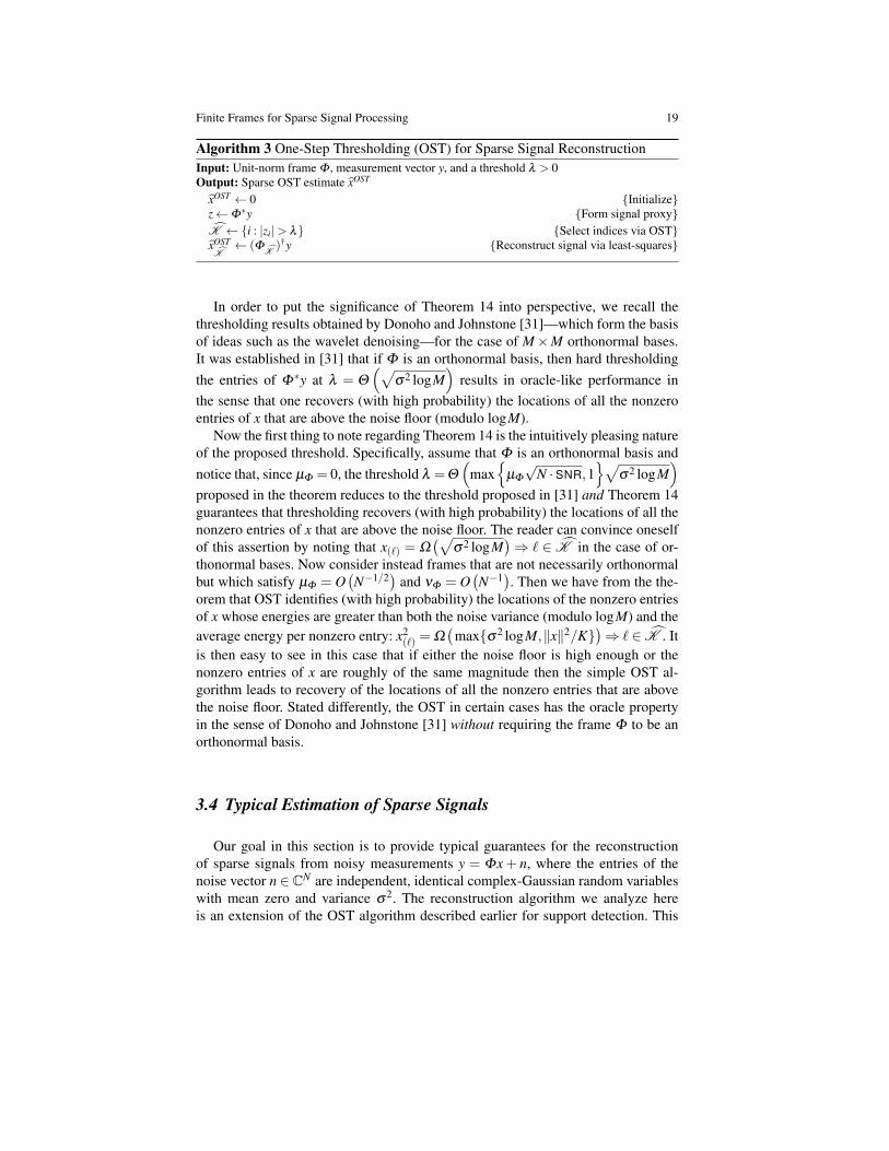
In light of these concerns, a few researchers recently revisited the much older(and oft-forgotten) method of thresholding for support detection [2, 3, 37, 39, 57,61]. The One-Step Thresholding (OST) algorithm, described in Algorithm 2, hascomputational complexity of only O(NM) and it has been known to be nearly op-timal for M×M orthonormal bases [31]. In this subsection, we focus on a recentresult of Bajwa et al. [2, 3] concerning typical support detection using OST. The

18 Waheed U. Bajwa and Ali Pezeshki
Algorithm 2 The One-Step Thresholding (OST) Algorithm for Support DetectionInput: Unit-norm frame Φ , measurement vector y, and a threshold λ > 0Output: Estimate of signal support K ⊂ 1, . . . ,M
z←Φ∗y Form signal proxyK ←i ∈ 1, . . . ,M : |zi|> λ Select indices via OST
forthcoming theorem in this regard relies on a notion of the coherence property,defined below.
Definition 3 (The Coherence Property [2, 3]). We say a unit-norm frame Φ satis-fies the coherence property if
(CP-1) µΦ ≤ 0.1√2logM and (CP-2) νΦ ≤ µΦ√
N.
In words, (CP-1) roughly states that the frame elements of Φ are not too sim-ilar, while (CP-2) roughly states that the frame elements of a unit-norm Φ aresomewhat distributed within the N-dimensional unit ball. Note that the coher-ence property (i) does not require the singular values of the submatrices of Φ tobe bounded away from zero and (ii) can be verified in polynomial time since itsimply requires checking ‖GΦ − Id‖max ≤ (200logM)−1/2 and ‖(GΦ − Id)1‖∞ ≤‖GΦ − Id‖max(M−1)N−1/2.
The implications of the coherence property are described in the following the-orem. Before proceeding further, however, we first define some notation. We useSNR
.= ‖x‖2/E[‖n‖2] to denote the signal-to-noise ratio associated with the sup-
port detection problem. Also, we use x(`) to denote the `-th largest (in magnitude)nonzero entry of x. We are now ready to state the typical support detection perfor-mance of the OST algorithm.
Theorem 14 ([3]). Suppose that y = Φx+ n for a K-sparse signal x ∈ CM whosesupport K is drawn uniformly at random. Further, let M ≥ 128, the noise n be dis-tributed as complex Gaussian with mean 0 and covariance σ2Id, n∼C N (0,σ2Id),and the frame Φ satisfy the coherence property. Finally, fix a parameter t ∈ (0,1)and choose the threshold
λ = max1
t10µΦ
√N · SNR,
11− t
√2√
2σ2 logM.
Then, under the assumption that K ≤N/(2logM), the OST algorithm (Algorithm 2)guarantees with probability exceeding 1− 6M−1 that K ⊂ K and
∣∣K \ K∣∣ ≤
(K−L), where L is the largest integer for which the following inequality holds:
x(L) > maxc8σ ,c9µΦ‖x‖√
logM. (20)
Here, c8.= 4(1− t)−1, c9
.= 20
√2 t−1, and the probability of failure is with respect
to the true model K and the Gaussian noise n.
Finite Frames for Sparse Signal Processing 19
Algorithm 3 One-Step Thresholding (OST) for Sparse Signal ReconstructionInput: Unit-norm frame Φ , measurement vector y, and a threshold λ > 0Output: Sparse OST estimate xOST
xOST ← 0 Initializez←Φ∗y Form signal proxyK ←i : |zi|> λ Select indices via OSTxOSTK← (Φ
K)†y Reconstruct signal via least-squares
In order to put the significance of Theorem 14 into perspective, we recall thethresholding results obtained by Donoho and Johnstone [31]—which form the basisof ideas such as the wavelet denoising—for the case of M×M orthonormal bases.It was established in [31] that if Φ is an orthonormal basis, then hard thresholdingthe entries of Φ∗y at λ = Θ
(√σ2 logM
)results in oracle-like performance in
the sense that one recovers (with high probability) the locations of all the nonzeroentries of x that are above the noise floor (modulo logM).
Now the first thing to note regarding Theorem 14 is the intuitively pleasing natureof the proposed threshold. Specifically, assume that Φ is an orthonormal basis andnotice that, since µΦ = 0, the threshold λ =Θ
(max
µΦ
√N · SNR,1
√σ2 logM
)proposed in the theorem reduces to the threshold proposed in [31] and Theorem 14guarantees that thresholding recovers (with high probability) the locations of all thenonzero entries of x that are above the noise floor. The reader can convince oneselfof this assertion by noting that x(`) = Ω
(√σ2 logM
)⇒ ` ∈ K in the case of or-
thonormal bases. Now consider instead frames that are not necessarily orthonormalbut which satisfy µΦ = O
(N−1/2
)and νΦ = O
(N−1
). Then we have from the the-
orem that OST identifies (with high probability) the locations of the nonzero entriesof x whose energies are greater than both the noise variance (modulo logM) and theaverage energy per nonzero entry: x2
(`) = Ω(
maxσ2 logM,‖x‖2/K)⇒ ` ∈ K . It
is then easy to see in this case that if either the noise floor is high enough or thenonzero entries of x are roughly of the same magnitude then the simple OST al-gorithm leads to recovery of the locations of all the nonzero entries that are abovethe noise floor. Stated differently, the OST in certain cases has the oracle propertyin the sense of Donoho and Johnstone [31] without requiring the frame Φ to be anorthonormal basis.
3.4 Typical Estimation of Sparse Signals
Our goal in this section is to provide typical guarantees for the reconstructionof sparse signals from noisy measurements y = Φx+ n, where the entries of thenoise vector n ∈CN are independent, identical complex-Gaussian random variableswith mean zero and variance σ2. The reconstruction algorithm we analyze hereis an extension of the OST algorithm described earlier for support detection. This

20 Waheed U. Bajwa and Ali Pezeshki
OST algorithm for reconstruction is described in Algorithm 3, and has been recentlyanalyzed in [4]. The following theorem is due to Bajwa et al. [4] and shows thatthe OST algorithm leads to near-optimal reconstruction error for certain importantclasses of sparse signals.
Before a formal statement of the theorem, however, we need to define some morenotation. We use Tσ (t) := i : |xi|> 2
√2
1−t
√2σ2 logM for any t ∈ (0,1) to denote
the locations of all the entries of x that, roughly speaking, lie above the noise floorσ . Also, we use Tµ(t) := i : |xi|> 20
t µΦ‖x‖√
2logM to denote the locations ofentries of x that, roughly speaking, lie above the self-interference floor µΦ‖x‖. Fi-nally, we also need a stronger version of the coherence property for reconstructionguarantees.
Definition 4 (The Strong Coherence Property [3]). We say a unit norm frame Φ
satisfies the strong coherence property if
(SCP-1) µΦ ≤ 1164logM and (SCP-2) νΦ ≤ µΦ√
N.
Theorem 15 ([4]). Take a unit-norm frame Φ which satisfies the strong coherenceproperty, pick t ∈ (0,1), and choose λ =
√2σ2 logM max 10
t µΦ
√N SNR,
√2
1−t .Further, suppose x ∈ CM has support K drawn uniformly at random from all pos-sible K-subsets of 1, . . . ,M. Then provided
K ≤ Mc2
10‖Φ‖2 logM, (21)
Algorithm 3 produces K such that Tσ (t)∩Tµ(t)⊆ K ⊆K and xOST such that
‖x− xOST‖ ≤ c11
√σ2|K | logM+ c12‖xK \K ‖ (22)
with probability exceeding 1− 10M−1. Finally, defining T := |Tσ (t)∩Tµ(t)|, wefurther have
‖x− x‖ ≤ c11√
σ2K logM+ c12‖x− xT‖ (23)
in the same probability event. Here, c10 = 37e, c11 =2
1−e−1/2 , and c12 = 1+ e−1/2
1−e−1/2
are numerical constants.
A few remarks are in order now for Theorem 15. First, if Φ satisfies the strongcoherence property and Φ is nearly tight, then OST handles sparsity that is almostlinear in N: K = O(N/ logM) from (21). Second, the `2 error associated with theOST algorithm is the near-optimal (modulo the log factor) error of
√σ2K logM
plus the best T -term approximation error caused by the inability of the OST al-gorithm to recover signal entries that are smaller than O(µΦ‖x‖
√2logM). In par-
ticular, if the K-sparse signal x, the worst-case coherence µΦ , and the noise n to-gether satisfy ‖x− xT‖ = O(
√σ2K logM), then the OST algorithm succeeds with
a near-optimal `2 error of ‖x− x‖= O(√
σ2K logM). To see why this error isnear-optimal, note that a K-dimensional vector of random entries with mean zero

Finite Frames for Sparse Signal Processing 21
and variance σ2 has expected squared norm σ2K; in here, the OST pays an ad-ditional log factor to find the locations of the K nonzero entries among the en-tire M-dimensional signal. It is important to recognize that the optimality condition‖x−xT‖= O(
√σ2K logM) depends on the signal class, the noise variance, and the
worst-case coherence of the frame; in particular, the condition is satisfied whenever‖xK \Tµ (t)‖= O(
√σ2K logM), since
‖x− xT‖ ≤ ‖xK \Tσ (t)‖+‖xK \Tµ (t)‖= O(√
σ2K logM)+‖xK \Tµ (t)‖. (24)
We conclude this subsection by stating a lemma from [4] that provides classes ofsparse signals which satisfy ‖xK \Tµ (t)‖= O(
√σ2K logM) given sufficiently small
noise variance and worst-case coherence.
Lemma 3. Take a unit-norm frame Φ with worst-case coherence µΦ ≤ c13√N
forsome c13 > 0, and suppose that K ≤ M
c214‖Φ‖2 logM
for some c14 > 0. Fix a con-stant β ∈ (0,1], and suppose the magnitudes of βK nonzero entries of x are someα = Ω(
√σ2 logM), while the magnitudes of the remaining (1−β )K nonzero en-
tries are not necessarily same, but are smaller than α and scale as O(√
σ2 logM).Then ‖xK \Tµ (t)‖= O(
√σ2K logM), provided c13 ≤ tc14
20√
2.
In words, Lemma 3 states that OST is near-optimal for those K-sparse signalswhose entries above the noise floor have roughly the same magnitude. This sub-sumes a very important class of signals that appears in applications such as multi-label prediction [47], in which all the nonzero entries take values ±α .
4 Finite Frames for Detecting the Presence of Sparse Signals
In the previous sections, we discussed the role of frame theory in recovering andestimating sparse signals in different settings. We now consider a different problem,namely the problem of detecting the presence of a sparse signal in noise. In thesimplest form, the problem is to decide whether an observed data vector is a realiza-tion from a hypothesized noise-only model or from a hypothesized signal-plus-noisemodel, where in the latter model the signal is sparse but the indices and the valuesof its nonzero elements are unknown. The problem is a binary hypothesis test of theform
H0 : y = ΦnH1 : y = Φ(x+n) , (25)
where x ∈ RM is a deterministic but unknown K-sparse signal, the measurementmatrix Φ = ϕiM
i=1 is a frame for RN , N ≤M, which we get to design, and n ∈RM
is a white Gaussian noise vector with covariance matrix E[nnT ] = (σ2n /M)Id.
We assume here that the number of measurements N allowed for detection isfixed and pre-specified. We wish to decide whether the measurement vector y ∈ RN
belongs to model H0 or H1. This problem is fundamentally different from that of

22 Waheed U. Bajwa and Ali Pezeshki
estimating a sparse signal, as the objective in detection typically is to maximize theprobability of detection, while maintaining a low false alarm rate, or to minimizethe total error probability or a Bayes risk, rather than to find the sparsest signal thatfits a linear observation model. Unlike the signal estimation problem, the detectionof sparse signals has received very little attention so far, with notable exceptionsbeing [45, 56, 74]. But in particular, the design of optimal or near-optimal compres-sive measurement matrices for detection of sparse signals has only been scarcelyaddressed [76, 77]. In this section, we provide an overview of selected results byZahedi et al. [76, 77], concerning the necessary and sufficient conditions for a frameΦ to optimize a measure of detection performance.
We look at the general problem of designing the measurement frame Φ to maxi-mize the measurement signal-to-noise ratio (SNR), under H1, which is given by
SNR =‖Φx‖2
σ2n /M
. (26)
This is motivated by the fact that for the class of linear log-likelihood ratio detectors,where the log-likelihood ratio is a linear function of the data, the detection perfor-mance is improved by increasing SNR. In particular, for a Neyman-Pearson detector(see, e.g., [60]) with false alarm rate PF ≤ γ , the probability of detection
Pd = Q(Q−1(γ)−√
SNR) (27)
is monotonically increasing in SNR, where Q(·) is the Q-function, given by
Q(z) =∞∫
z
e−w2/2dw. (28)
In addition, maximizing SNR leads to maximum detection probability at a pre-specified false alarm rate in an energy detector, which simply tests the energy ofthe measured vector y against a threshold. Without loss of generality, we assumethat σ2
n = 1 and ‖x‖2 = 1, and we design Φ to maximize the measured signal en-ergy ‖Φx‖2. To avoid coloring the noise vector n, that is, to keep the noise vectorwhite, we constrain the measurement frame Φ to be Parseval, or tight with framebound equal to one. That is, we only consider frames for which the frame opera-tor SΦ = ΦΦT is identity. From here on we simply refer to these frames as tightframes, but it is understood that all tight frames we consider in this section are infact Parseval.
In solving the problem, one approach is to assume a value for the sparsity levelK and design the measurement frame Φ based on this assumption. This approach,however, runs the risk that the true sparsity level might be different. An alternativeapproach is not to assume any specific sparsity level. Instead, when designing Φ ,we prioritize the level of importance of different values of sparsity. In other words,we first find a set of solutions that are optimal for a K1-sparse signal. Then, withinthis set, we find a subset of solutions that are also optimal for K2-sparse signals. We

Finite Frames for Sparse Signal Processing 23
follow this procedure until we find a subset that contains a family of optimal solu-tions for sparsity levels K1, K2, K3, · · · . This approach is known as a lexicographicoptimization method (see, e.g., [33, 43, 48]). The measurement frame design natu-rally depends on one’s assumptions about the unknown vector x. In the subsequentsection, we review two different design problems, namely a worst-case SNR designand an average SNR design, following the developments of [76, 77].
We note that lexicographic optimizations have been employed earlier in [46] inthe design of frames that have maximal robustness to erasures of frame coefficients.The analysis used in deriving the main results for the worst-case SNR design issimilar in nature to that used in [46].
4.1 Wort-Case SNR Design
In the worst-case design for a sparsity level K, we consider the vector x that mini-mizes the SNR among all K-sparse signals and design the frame Φ to maximize thisminimum SNR. Of course, when minimizing the SNR with respect to x, we haveto find the minimum SNR with respect to both the locations and the values of thenonzero entries in x. To combine this with the lexicographic approach, we design thematrix Φ to maximize the worst-case detection SNR, where the worst-case is takenover all subsets of size Ki of elements of x, where Ki is the sparsity level consideredat the ith level of lexicographic optimization. This is a design for robustness withrespect to the worst sparse signal that can be produced.
Consider the Kth step of the lexicographic approach. In this step, the vector x isassumed to have up to K nonzero entries, and we assume ‖x‖2 = 1. But otherwise,we do not impose any constraints on the locations and the values of the nonzeroentries of x. We wish to maximize the minimum (worst-case) SNR, produced byassigning the worst possible locations and values to the nonzero entries of the K-sparse vector x. Since we assume σ2
n = 1, this corresponds to a worst-case designfor maximizing the signal energy ‖Φx‖2.
Let B0 be the set containing all (N×M) tight frames. We recursively define theset BK , K = 1,2, . . ., as the set of solutions to the following worst-case optimizationproblem [77]:
maxΦ
minx‖Φx‖2,
s.t. Φ ∈BK−1,‖x‖= 1,x is K-sparse.
(29)
The optimization problem for the Kth stage (29) involves a worst-case objective re-stricted to the set of solutions BK−1 from the (K−1)th problem. So, BK ⊂BK−1 ⊂·· · ⊂B0.
Now let Ω = 1,2, . . . ,M, and define ΩK to be ΩK = ω ⊂ Ω : |ω|= K. Forany T ∈ΩK , let xT be the subvector of size (K×1) that contains all the componentsof x corresponding to indices in T . Similarly, given a frame Φ , let ΦT be the
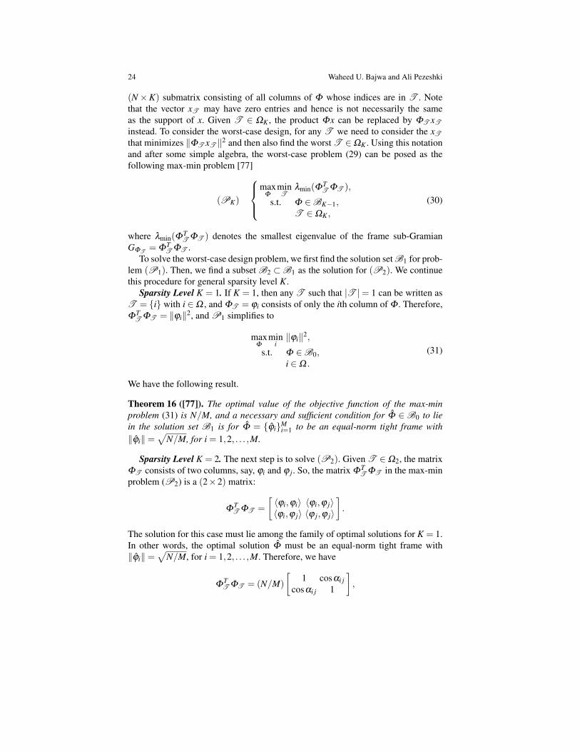
24 Waheed U. Bajwa and Ali Pezeshki
(N×K) submatrix consisting of all columns of Φ whose indices are in T . Notethat the vector xT may have zero entries and hence is not necessarily the sameas the support of x. Given T ∈ ΩK , the product Φx can be replaced by ΦT xT
instead. To consider the worst-case design, for any T we need to consider the xT
that minimizes ‖ΦT xT ‖2 and then also find the worst T ∈ΩK . Using this notationand after some simple algebra, the worst-case problem (29) can be posed as thefollowing max-min problem [77]
(PK)
max
ΦminT
λmin(ΦTT ΦT ),
s.t. Φ ∈BK−1,T ∈ΩK ,
(30)
where λmin(ΦTT ΦT ) denotes the smallest eigenvalue of the frame sub-Gramian
GΦT= ΦT
T ΦT .To solve the worst-case design problem, we first find the solution set B1 for prob-
lem (P1). Then, we find a subset B2 ⊂B1 as the solution for (P2). We continuethis procedure for general sparsity level K.
Sparsity Level K = 1. If K = 1, then any T such that |T |= 1 can be written asT = i with i ∈Ω , and ΦT = ϕi consists of only the ith column of Φ . Therefore,ΦT
T ΦT = ‖ϕi‖2, and P1 simplifies to
maxΦ
mini‖ϕi‖2,
s.t. Φ ∈B0,i ∈Ω .
(31)
We have the following result.
Theorem 16 ([77]). The optimal value of the objective function of the max-minproblem (31) is N/M, and a necessary and sufficient condition for Φ ∈B0 to liein the solution set B1 is for Φ = ϕiM
i=1 to be an equal-norm tight frame with‖ϕi‖=
√N/M, for i = 1,2, . . . ,M.
Sparsity Level K = 2. The next step is to solve (P2). Given T ∈Ω2, the matrixΦT consists of two columns, say, ϕi and ϕ j. So, the matrix ΦT
T ΦT in the max-minproblem (P2) is a (2×2) matrix:
ΦTT ΦT =
[〈ϕi,ϕi〉 〈ϕi,ϕ j〉〈ϕi,ϕ j〉 〈ϕ j,ϕ j〉
].
The solution for this case must lie among the family of optimal solutions for K = 1.In other words, the optimal solution Φ must be an equal-norm tight frame with‖ϕi‖=
√N/M, for i = 1,2, . . . ,M. Therefore, we have
ΦTT ΦT = (N/M)
[1 cosαi j
cosαi j 1
],
Finite Frames for Sparse Signal Processing 25
where αi j is the angle between vectors ϕi and ϕ j. The minimum possible eigenvalueof this matrix is
λmin(ΦTT ΦT ) = (N/M)(1−µΦ). (32)
where µΦ is the worst-case coherence of the frame Φ = ϕiMi=1 ∈B1, as defined
in (1).Now, let µmin be the minimum worst-case coherence
µmin = minΦ∈B1
µΦ (33)
for all frames in B1. We refer to the element of B1 that has the worst-case coherenceµmin as a Grassmannian equal-norm tight frame.
We have the following theorem.
Theorem 17 ([77]). The optimal value of the objective function of the max-minproblem (P2) is (N/M)(1− µmin). A frame Φ is in B2 if and only if the columnsof Φ form an equal-norm tight frame with norm values
√N/M and µ
Φ= µmin.
In other words, the solution to (P2) is an N×M Grassmannian equal-norm tightframe.
Sparsity Level K > 2. We now consider the case where K > 2. In this case, T ∈ΩK can be written as T = i1, i2, . . . , iK ⊂Ω . From the previous results, we knowthat an optimal frame Φ ∈ BK must be a Grassmannian equal-norm tight frame,with norms
√N/M and worst-case coherence µmin.Taking this into account, the
(K×K) matrix ΦTT ΦT in (PK), K > 2, can be written as ΦT
T ΦT = (N/M)[Id +AT ] where AT is given by
AT =
0 cos αi1i2 . . . cos αi1ik
cos αi1i2 0 . . . cos αi2ik...
.... . .
...cos αi1ik cos αi2ik . . . 0
, (34)
and cos αihi f is the cosine of the angle between frame elements ϕih and ϕi f , ih 6= i f ∈T . It is easy to see that
λmin(ΦTT ΦT ) = (N/M)(1+λmin(AT )). (35)
So, the problem (PK), K > 2, simplifies to
(PK)
max
ΦminT
λmin(AT ),
s.t. Φ ∈BK−1,T ∈ΩK .
(36)
Solving the above problem however is not trivial. But we can at least bound theoptimum value. Given T ∈ΩK , let δihi f and ∆min be

26 Waheed U. Bajwa and Ali Pezeshki
δihi f = µmin−|cosαihi f |, ih 6= i f ∈T , (37)
∆min = minT ∈ΩK
∑ih 6=i f∈T
δihi f . (38)
Also, define ∆ in the following way:
∆ = minT ∈ΩK
∑ih 6=i f∈T
δihi f .
We have the following theorem.
Theorem 18 ([77]). The optimal value of the objective function of the max-minproblem (PK) for K > 2 lies between (N/M)(1−
(K2
)µmin +∆min) and (N/M)(1−
µmin).
Before we conclude the worst-case SNR design, a few remarks are in order.
1. Examples of uniform tight frames and their methods of construction can be foundin [8, 13, 19, 20], and the references therein.
2. In the case where K = 2, ΦTT ΦT associated with the frame Φ identified in The-
orem 17, has the largest minimum eigenvalue (N/M)(1−µmin) and the smallestmaximum eigenvalue (N/M)(1+ µmin) among all Φ ∈B1 and T ∈ Ω2. Thismeans that the solution Φ to (P2) is an RIP matrix of order 2 with optimal RICδ2 = µmin.
3. In general, the minimum worst-case coherence µmin of the solution Φ to (PK),K ≥ 2, is bounded below by the Welch bound (see Lemma 2). However, when1≤ N ≤M−1 and
M ≤minN(N +1)/2,(M−N)(M−N +1)/2 (39)
the Welch bound can be met [64]. For such a case, all frame angles are equal andthe solution to (PK) for K ≥ 2 is an equiangular equal-norm tight frame. Suchframes are Grassmannian line packings (see, e.g., [8, 21, 24, 49, 52, 58, 63, 64,65]).
4.2 Average-Case Design
Let us now assume that in (25) the locations of nonzero entries of x are randombut their values are deterministic and unknown. We wish to find the frame Φ thatmaximizes the expected value of the minimum SNR. The expectation is taken withrespect to a random index set with uniform distribution over the set of all possiblesubsets of size Ki of the index set 1,2, . . . ,M of elements of x. The minimumSNR, whose expected value we wish to maximize, is calculated with respect to thevalues of the entries of the vector x for each realization of the random index set.

Finite Frames for Sparse Signal Processing 27
Let TK be a random variable that is uniformly distributed over ΩK . ThenpTK (t) = 1/
(MK
)is the probability that TK = t for t ∈ΩK . Our goal is to find a mea-
surement frame Φ that maximizes the expected value of the minimum SNR, wherethe expectation is taken with respect to the random TK , and the minimum is takenwith respect to the entries of the vector x on TK . Taking into account the simplify-ing steps used earlier for the worst-case problem and also adopting the lexicographicapproach, the problem of maximizing the average SNR can then be formulated inthe following way.
Let N0 be the set containing all (N ×M) tight frames. Then for K = 1,2, . . . ,recursively define the set NK as the solution set to the following optimization prob-lem:
maxΦ
ETK minxK‖ΦTK xK‖2,
s.t. Φ ∈NK−1,‖xK‖= 1,
(40)
where ETK is the expectation with respect to TK . As before, the (N ×K) matrixΦTK is a submatrix of Φ whose column indices are in TK . The above problem canbe simplified to the following [77]:
(FK)
max
ΦETK λmin(Φ
TTK
ΦTK ),
s.t. Φ ∈NK−1.(41)
To solve the lexicographic problems (FK), we follow the same method we usedearlier for the worst-case problem, i.e., we begin by solving problem (F1). Then,from the solution set N1, we find optimal solutions for the problem (F2), and soon.
Sparsity Level K = 1. Assume that the signal x is 1-sparse. So, there are(M
1
)= M
different possibilities to build the matrix ΦT1 from the matrix Φ . The expectationin problem (F1) can be written as:
ET1λmin(ΦTT1
ΦT1) = ∑t∈Ω1
pT1(t)λmin(ΦTt Φt) =
M
∑i=1
pT1(i)‖ϕi‖2 =NM. (42)
The following result holds.
Theorem 19 ([77]). The optimal value of the objective function of problem (F1) isN/M. This value is obtained by using any Φ ∈N0, i.e., any tight frame.
Theorem 19 shows that unlike the worst-case problem, any tight frame is anoptimal solution for the problem (F1). Next, we study the case where the signal xis 2-sparse.
Sparsity Level K = 2. For problem (F2), the expected value term ET2λmin(ΦTT2
ΦT2)is equal to
∑t∈Ω2
pT2(t)λmin(ΦTt Φt) =
2M(M−1)
M
∑j=2
j−1
∑i=1
λmin(ΦTi, jΦi, j). (43)

28 Waheed U. Bajwa and Ali Pezeshki
In general, solving the family of problems (FK), K = 2,3, . . . , is not trivial. How-ever, if we constrain ourselves to the class of equal-norm tight frames, which alsoarise in solving the worst-case problem, we can establish necessary and sufficientconditions for optimality. These conditions are different from those for the worst-case problem and as we will show next the optimal solution here is an equal-normtight frame for which a cumulative measure of coherence is minimal.
Let M1 be defined as M1 = Φ : Φ ∈N1,‖ϕi‖ =√
N/M,∀i ∈ Ω. Also, forK = 2,3, . . . , recursively define the set MK as the solution set to the following opti-mization problem:
(F′K)
max
ΦETK λmin(Φ
TTK
ΦTK ),
s.t. Φ ∈MK−1.(44)
We will concentrate on solving the above family of problems instead of (FK), K =2,3, . . .. We have the following results.
Theorem 20 ([77]). The frame Φ is in M2 if and only if the sum coherence of Φ ,i.e., ∑
Mj=2 ∑
j−1i=1 |〈ϕi,ϕ j〉|/(‖ϕi‖‖ϕ j‖), is minimized.
Theorem 20 shows that for problem (F′2), angles between elements of the equal-
norm tight frame Φ should be designed in a different way than for the worst-caseproblem. For example, an equiangular tight frame of M = 2N in N dimensions, withvectors of equal norm
√1/2, has worst-case coherence 1/(2
√2N−1) and sum co-
herence N√
2N−1/2, while two copies of an orthonormal basis form a frame withworst-case coherence 1/2 and sum coherence N/2. While it is not clear whethercopies of orthonormal bases form tight frames with minimal sum coherence, thisexample certainly illustrates that Grassmannian frames do not, in general, result inminimal sum coherence. To the best of our knowledge, no general method for con-structing tight frames with minimal sum coherence has been proposed so far.
The following lemma provides bounds on the sum coherence of an equal-normtight frame.
Lemma 4 ([77]). For an equal-norm tight frame Φ with norm values√
N/M, thefollowing inequalities hold:
c|(M/N−1)−2(M−1)µ2Φ | ≤
M
∑j=2
j−1
∑i=1|〈ϕi,ϕ j〉| ≤ c(M−1)µ2
Φ ,
where
c =(
(N/M)2
1−2(N/M)
)(M(M−2)
2
).
Sparsity Level K > 2. Similar to the worst-case problem, solving problems (F′K)
for K > 2 is not trivial. This is because the solution sets for these problems all liein M2, and (F
′2) is still an open problem. The following lemma provides a lower
bound for the optimal objective function of (F′K), K > 2.

Finite Frames for Sparse Signal Processing 29
Lemma 5 ([77]). The optimal value of the objective function for problem (F′K),
K > 2, is bounded below by (N/M)(1− (K(K−1)/2)µΦ).
We conclude this section by giving a summary. In the worst-case SNR prob-lem, the optimal measurement matrix is a Grassmannian equal-norm tight frame formost—and a equal-norm tight frame for all—sparse signals. In the average SNRproblem, we limited ourselves to the class of equal-norm tight frames and showedthat the optimal measurement frame is an equal-norm tight frame that has minimumsum coherence.
5 Other Topics
As mentioned earlier, this chapter covers only a small subset of the results in thesparse signal processing literature. Our aim has been to simply highlight the centralrole that finite frames and their geometric measures, such as spectral norm, worst-case coherence, average coherence, and sum coherence, play in the developmentof sparse signal processing methods. But many developments, which also involvefinite frames, have not been covered. For example, there is a large body of workon signal processing of compressible signals. These are signals that are not sparse,but their entries decay in magnitude according to a particular power law. Many ofthe results covered in this chapter on estimating sparse signals have counterpartsfor compressible signals. The reader is referred to [17, 23, 26, 27] for examplesof such results. Another example is the estimation and recovery of block-sparsesignals, where the nonzero entries of the signal to be estimated are either clusteredor the signal has a sparse representation in a fusion frame. Again, the majority of theresults on the estimation and recovery of sparse signals can be extended to block-sparse signals. The reader is referred to [9, 35, 62, 78] and the references therein.
References
1. IEEE signal processing mag., special issue on compressive sampling (2008)2. Bajwa, W.U., Calderbank, R., Jafarpour, S.: Model selection: Two fundamental measures of
coherence and their algorithmic significance. In: Proc. IEEE Intl. Symp. Information Theory(ISIT’10), pp. 1568–1572. Austin, TX (2010)
3. Bajwa, W.U., Calderbank, R., Jafarpour, S.: Why Gabor frames? Two fundamental measuresof coherence and their role in model selection. J. Commun. Netw. 12(4), 289–307 (2010)
4. Bajwa, W.U., Calderbank, R., Mixon, D.G.: Two are better than one: Fundamental parametersof frame coherence. Appl. Comput. Harmon. Anal. (2011). DOI doi:10.1016/j.acha.2011.09.005. URL http://arxiv.org/abs/1103.0435. In press
5. Bajwa, W.U., Haupt, J., Raz, G., Nowak, R.: Compressed channel sensing. In: Proc. 42ndAnnu. Conf. Information Sciences and Systems (CISS’08), pp. 5–10. Princeton, NJ (2008)
6. Ben-Haim, Z., Eldar, Y.C., Elad, M.: Coherence-based perfromance guarantees for estimatinga sparse vector under random noise. IEEE Trans. Signal Processing 58(10), 5030–5043 (2010)
7. Blumensath, T., Davies, M.E.: Iterative hard thresholding for compressed sensing. Appl. Com-put. Harmon. Anal. 27(3), 265–274 (2009)

30 Waheed U. Bajwa and Ali Pezeshki
8. Bodmann, B.G., Paulsen, V.I.: Frames, graphs and erasures. Linear Algebra and its Applica-tions 404, 118–146 (2005)
9. Boufounos, P., Kutynio, G., Rahut, H.: Sparse recovery from combined fusion frame measure-ments. IEEE Trans. Info. Theory 57(6), 3864–3876 (2011)
10. Bourgain, J., Dilworth, S.J., Ford, K., Konyagin, S.V., Kutzarova, D.: Breaking the k2 barrierfor explicit RIP matrices. In: Proc. 43rd Annu. ACM Symp. Theory Computing (STOC’11),pp. 637–644. San Jose, California (2011)
11. Boyd, S., Vandenberghe, L.: Convex Optimization. Cambridge University Press, Cambridge,U.K. (2004)
12. Bruckstein, A.M., Donoho, D.L., Elad, M.: From sparse solutions of systems of equations tosparse modeling of signals and images. SIAM Review 51(1), 34–81 (2009)
13. Calderbank, R., Casazza, P., Heinecke, A., Kutyniok, G., Pezeshki, A.: Sparse fusion frames:existence and construction. Advances in Computational Mathematics 35, 1–31 (2011)
14. Candes, E.J.: The restricted isometry property and its implications for compressed sensing.In: C. R. Acad. Sci., Ser. I, vol. 346, pp. 589–592. Paris (2008)
15. Candes, E.J., Plan, Y.: Near-ideal model selection by `1 minimization. Ann. Statist. 37(5A),2145–2177 (2009)
16. Candes, E.J., Romberg, J., Tao, T.: Robust uncertainty principles: Exact signal reconstructionfrom highly incomplete frequency information. IEEE Trans. Inform. Theory 52(2), 489–509(2006)
17. Candes, E.J., Tao, T.: Near-optimal signal recovery from random projections: Universal en-coding strategies? IEEE Trans. Inform. Theory 52(12), 5406–5425 (2006)
18. Candes, E.J., Tao, T.: The Dantzig selector: Statistical estimation when p is much larger thann. Ann. Statist. 35(6), 2313–2351 (2007)
19. Casazza, P., Fickus, M., Mixon, D., Wang, Y., Zhou, Z.: Constructing tight fusion frames.Applied and Computational Harmonic Analysis 30, 175–187 (2011)
20. Casazza, P., Leon, M.: Existence and construction of finite tight frames. J. Concr. Appl. Math4(3), 277–289 (2006)
21. Casazza, P.G., Kovacevic, J.: Equal-norm tight frames with erasures. Appl. Comput. Harmon.Anal. 18(2–4), 387–430 (2003)
22. Chen, S.S., Donoho, D.L., Saunders, M.A.: Atomic decomposition by basis pursuit. SIAM J.Scientific Comput. 20(1), 33–61 (1998)
23. Cohen, A., Dahmen, W., Devore, R.A.: Compressed sensing and best k-term approximation.J. Amer. Math. Soc. 22(1), 211–231 (2009)
24. Conway, J.H., Hardin, R.H., Sloane, N.J.A.: Packing lines, planes, etc.: Packings in Grass-mannian spaces. Experimental Mathematics 5(2), 139–159 (1996)
25. Dai, W., Milenkovic, O.: Subspace pursuit for compressive sensing signal reconstruction.IEEE Trans. Inform. Theory 55(5), 2230–2249 (2009)
26. Devore, R.A.: Nonlinear approximation. In: A. Iserles (ed.) Acta Numerica, vol. 7, pp. 51–150. Cambridge University Press, Cambridge, U.K. (1998)
27. Donoho, D.L.: Compressed sensing. IEEE Trans. Inform. Theory 52(4), 1289–1306 (2006)28. Donoho, D.L., Elad, M.: Optimally sparse representation in general (nonorthogonal) dictio-
naries via `1 minimization. Proc. Natl. Acad. Sci. 100(5), 2197–2202 (2003)29. Donoho, D.L., Elad, M., Temlyakov, V.N.: Stable recovery of sparse overcomplete represen-
tations in the presence of noise. IEEE Trans. Inform. Theory 52(1), 6–18 (2006)30. Donoho, D.L., Huo, X.: Uncertainty principles and ideal atomic decomposition. IEEE Trans.
Inform. Theory 47(7), 2845–2862 (2001)31. Donoho, D.L., Johnstone, I.M.: Ideal spatial adaptation by wavelet shrinkage. Biometrika
81(3), 425–455 (1994)32. Efron, B., Hastie, T., Johnstone, I., Tibshirani, R.: Least angle regression. Ann. Statist. 32(2),
407–451 (2004)33. Ehrgott, M.: Multicriteria Optimization, 2nd edn. Springer (2005)34. Eldar, Y., Kutyniok, G.: Compressed Sensing: Theory and Applications. Cambridge Univer-
sity Press (in press)

Finite Frames for Sparse Signal Processing 31
35. Eldar, Y.C., Kuppinger, P., Bolcskei, H.: Block-sparse signals: Uncertainty relations and effi-cient recovery. IEEE Trans. Signal Processing 58(6), 3042–3054 (2010)
36. Fickus, M., Mixon, D.G., Tremain, J.C.: Steiner equiangular tight frames. Linear AlgebraAppl. (2011). DOI 10.1016/j.laa.2011.06.027
37. Fletcher, A.K., Rangan, S., Goyal, V.K.: Necessary and sufficient conditions for sparsity pat-tern recovery. IEEE Trans. Inform. Theory 55(12), 5758–5772 (2009)
38. Foster, D.P., George, E.I.: The risk inflation criterion for multiple regression. Ann. Statist.22(4), 1947–1975 (1994)
39. Genovese, C., Jin, J., Wasserman, L.: Revisiting marginal regression (2009). URLhttp://arxiv.org/abs/0911.4080. Submitted for publication (arXiv:0911.4080v1[math.ST])
40. Gersgorin, S.A.: Uber die Abgrenzung der Eigenwerte einer Matrix. Izv. Akad. Nauk SSSRSer. Fiz.-Mat. 6, 749–754 (1931)
41. Gorodnitsky, I.F., Rao, B.D.: Sparse signal reconstruction from limited data using FOCUSS: Are-weighted minimum norm algorithm. IEEE Trans. Signal Processing 45(3), 600–616 (1997)
42. Gribonval, R., Nielsen, M.: Sparse representations in unions of bases. IEEE Trans. Inform.Theory 49(12), 3320–3325 (2003)
43. Hajek, B., Seri, P.: Lex-optimal online multiclass scheduling with hard deadlines. Mathemat-ics of Operations Research 30(3), 562–596 (2005)
44. Haupt, J., Bajwa, W.U., Raz, G., Nowak, R.: Toeplitz compressed sensing matrices with appli-cations to sparse channel estimation. IEEE Trans. Inform. Theory 56(11), 5862–5875 (2010)
45. Haupt, J., Nowak, R.: Compressive sampling for signal detection. In: Proc. IEEE InternationalConference on Acoustics, Speech and Signal Processing (ICASSP), vol. 3, pp. III–1509–III–1512 (2007)
46. Holmes, R.B., Paulsen, V.I.: Optimal frames for erasures. Linear Algebra and its Applications377(15), 31–51 (2004)
47. Hsu, D., Kakade, S., Langford, J., Zhang, T.: Multi-label prediction via compressed sensing.In: Advances in Neural Information Processing Systems, pp. 772–780 (2009)
48. Isermann, H.: Linear lexicographic optimization. OR Spectrum 4(4), 223–228 (1982)49. Kutyniok, G., Pezeshki, A., Calderbank, R., Liu, T.: Robust dimension reduction, fusion
frames, and Grassmannian packings. Appl. Comput. Harmon. Anal. 26(1), 64–76 (2009)50. Lancaster, P., Tismenetsky, M.: The Theory of Matrices, second edn. Academic Press, Or-
lando, FL (1985)51. Mallat, S.G., Zhang, Z.: Matching pursuits with time-frequency dictionaries. IEEE Trans.
Signal Processing 41(12), 3397–3415 (1993)52. Malozemov, V.N., Pevnyi, A.B.: Equiangular tight frames. Journal of Mathematical Sciences
157(6), 789–815 (2009)53. Meinshausen, N., Buhlmann, P.: High-dimensional graphs and variable selection with the
lasso. Ann. Statist. 34(3), 1436–1462 (2006)54. Natarajan, B.K.: Sparse approximate solutions to linear systems. SIAM J. Comput. 24(2),
227–234 (1995)55. Needell, D., Tropp, J.A.: CoSaMP: Iterative signal recovery from incomplete and inaccurate
samples. Appl. Comput. Harmon. Anal. 26(3), 301–321 (2009)56. Paredes, J., Wang, Z., Arce, G., Sadler, B.: Compressive matched subspace detection. In: Proc.
17th European Signal Processing Conference, pp. 120–124. Glasgow, Scotland (2009)57. Reeves, G., Gastpar, M.: A note on optimal support recovery in compressed sensing. In: Proc.
43rd Asilomar Conf. Signals, Systems and Computers. Pacific Grove, CA (2009)58. Renes, J.: Equiangular tight frames from Paley tournaments. Linear Algebra Appl. 426(2–3),
497–501 (2007)59. Santosa, F., Symes, W.W.: Linear inversion of band-limited reflection seismograms. SIAM J.
Sci. Statist. Comput. 7(4), 1307–1330 (1986)60. Scharf, L.L.: Statistical Signal Processing. Addison-Wesley, Cambridge, MA (1991)61. Schnass, K., Vandergheynst, P.: Average performance analysis for thresholding. IEEE Signal
Processing Lett. 14(11), 828–831 (2007)

32 Waheed U. Bajwa and Ali Pezeshki
62. Stojnic, M., Parvaresh, F., Hassibi, B.: On the representaton of block-sparse signals with anoptimal number of meausrements. IEEE Trans. Signal Processing 57(8), 3075–3085 (2009)
63. Strohmer, T.: A note on equiangular tight frames. Linear Algebra and its Applications 429(1),326–330 (2008)
64. Strohmer, T., Heath Jr., R.W.: Grassmannian frames with applications to coding and commu-nication. Appl. Comput. Harmon. Anal. 14(3), 257–275 (2003)
65. Sustik, M., Tropp, J.A., Dhillon, I.S., Heath Jr., R.W.: On the existence of equiangular tightframes. Linear Algebra Appl. 426(2–3), 619–635 (2007)
66. Tibshirani, R.: Regression shrinkage and selection via the lasso. J. Roy. Statist. Soc. Ser. B58(1), 267–288 (1996)
67. Tropp, J., Gilbert, A., Muthukrishnan, S., Strauss, M.: Improved sparse approximation overquasiincoherent dictionaries. In: Proc. IEEE Conf. Image Processing (ICIP’03), pp. 37–40(2003)
68. Tropp, J.A.: Greed is good: Algorithmic results for sparse approximation. IEEE Trans. Inform.Theory 50(10), 2231–2242 (2004)
69. Tropp, J.A.: Just relax: Convex programming methods for identifying sparse signals in noise.IEEE Trans. Inform. Theory 52(3), 1030–1051 (2006)
70. Tropp, J.A.: Norms of random submatrices and sparse approximation. In: C. R. Acad. Sci.,Ser. I, vol. 346, pp. 1271–1274. Paris (2008)
71. Tropp, J.A.: On the conditioning of random subdictionaries. Appl. Comput. Harmon. Anal.25, 1–24 (2008)
72. Tropp, J.A., Wright, S.J.: Computational methods for sparse solution of linear inverse prob-lems. Proc. IEEE 98(5), 948–958 (2010)
73. Wainwright, M.J.: Sharp thresholds for high-dimensional and noisy sparsity recovery using `1-constrained quadratic programming (lasso). IEEE Trans. Inform. Theory 55(5), 2183–2202(2009)
74. Wang, Z., Arce, G., Sadler, B.: Subspace compressive detection for sparse signals. In: IEEEInt. Conf. Acoust., Speech, Signal Process. (ICASSP), pp. 3873–3876 (2008)
75. Welch, L.: Lower bounds on the maximum cross correlation of signals. IEEE Trans. Inform.Theory 20(3), 397–399 (1974)
76. Zahedi, R., Pezeshki, A., Chong, E.K.P.: Robust measurement design for detecting sparse sig-nals: Equiangular uniform tight frames and Grassmannian packings. In: Proc. 2010 AmericanControl Conference (ACC). Baltimore, MD (2010)
77. Zahedi, R., Pezeshki, A., Chong, E.K.P.: Measurement design for detecting sparse signals.Physical Communications (2011). DOI 10.1016/j.phycom.2011.09.007
78. Zelnik-Manor, L., Rosenblum, K., Eldar, Y.C.: Sensing matrix optimization for block-sparsedecoding. IEEE Trans. Signal Processing 59(9), 4300–4312 (2011)
79. Zhao, P., Yu, B.: On model selection consistency of lasso. J. Machine Learning Res. 7, 2541–2563 (2006)

Index
basis pursuit, 7–10, 12–16denoising, see LASSOwith inequality constraint, 9, 10, 12
coherence, see frame coherencecoherence property, 18
strong coherence property, 20compressed sensing, 2, 12
square-root bottleneck, see square-rootbottleneck, sparse signal processing
frame coherenceaverage coherence, 3, 29sum coherence, 3, 28, 29worst-case coherence, 3–9, 12, 13, 15, 17,
20, 21, 25, 26, 28, 29
Gabor frame, 7, 14Gersgorin circle theorem, 5, 13Grassmannian frame, 4, 6–8, 12, 15, 25, 28Grassmannian line packings, 26
LASSO, 11, 12, 15–17
Neyman-Pearson detector, 22
one-step thresholding, 17–21orthogonal matching pursuit, 8–12
restricted isometry property, 12
spark, see unique representation propertysparse signal processing, 2–4, 7, 17, 29
square-root bottleneck, 12–16sparse signals
estimationaverage guarantees, 19–21uniform guarantees, 9–12
recoveryaverage guarantees, 13–15uniform guarantees, 4–9
regressionaverage guarantees, 15–16
signal detectionaverage design, 26–29worst-case SNR design, 23–26
support detectionaverage guarantees, 16–19
unique representation property, 5, 6
Welch bound, 6, 12, 26
33