Variational Autoencoders for Sparse and Overdispersed ...

Variational Autoencoders for Sparse and OverdispersedDiscrete Data

He Zhao∗ Piyush Rai† Lan Du∗

Wray Buntine∗ Dinh Phung∗ Mingyuan Zhou‡∗Faculty of Information Technology, Monash University, Australia

†Department of Computer Science and Engineering, IIT Kanpur, India‡McCombs School of Business, The University of Texas at Austin, USA

Abstract

Many applications, such as text modelling,high-throughput sequencing, and recom-mender systems, require analysing sparse,high-dimensional, and overdispersed discrete(count or binary) data. Recent deep proba-bilistic models based on variational autoen-coders (VAE) have shown promising resultson discrete data but may have inferior mod-elling performance due to the insufficientcapability in modelling overdispersion andmodel misspecification. To address these is-sues, we develop a VAE-based framework us-ing the negative binomial distribution as thedata distribution. We also provide an anal-ysis of its properties vis-a-vis other mod-els. We conduct extensive experiments onthree problems from discrete data analysis:text analysis/topic modelling, collaborativefiltering, and multi-label learning. Our mod-els outperform state-of-the-art approaches onthese problems, while also capturing the phe-nomenon of overdispersion more effectively.1

1 INTRODUCTION

Discrete data are ubiquitous in many applications. Forexample, in text analysis, a collection of documentscan be represented as a word-document count ma-trix; in recommender systems, users’ shopping history

1Code at https://github.com/ethanhezhao/NBVAE

Proceedings of the 23rdInternational Conference on Artifi-cial Intelligence and Statistics (AISTATS) 2020, Palermo,Italy. PMLR: Volume 108. Copyright 2020 by the au-thor(s).

can be represented as a binary (or count) item-usermatrix, with each entry indicating whether or not auser has bought an item (or its purchase count); inextreme multi-label learning problems, data samplescan be tagged with a large set of labels, presentedas a binary label matrix. Such kinds of data are of-ten characterised by high-dimensionality and extremesparsity. With the ability to handle high-dimensionaland sparse matrices, Probabilistic Matrix Factorisa-tion (PMF) (Mnih and Salakhutdinov, 2008) has beena key method of choice for such problems. PMF gen-erates data from a suitable probability distribution,parameterised by some low-dimensional latent factors.For modelling discrete data, Latent Dirichlet Alloca-tion (LDA) (Blei et al., 2003) and Poisson Factor Anal-ysis (PFA) (Canny, 2004; Zhou et al., 2012) are tworepresentative models that generate data samples us-ing the multinomial and Poisson distributions, respec-tively. Originally, LDA and PFA can be seen as single-layer models, whose modelling expressiveness may belimited. Several prior works have focused on extend-ing them with hierarchical/deep Bayesian priors (Bleiet al., 2010; Paisley et al., 2015; Gan et al., 2015b;Zhou et al., 2016; Lim et al., 2016; Zhao et al., 2018a).However, increasing model complexity with hierarchi-cal priors can also complicate inference, which hinderstheir usefulness in analysing large-scale data.

The recent success of deep generative models suchas Variational Autoencoders (VAEs) (Kingma andWelling, 2014; Rezende et al., 2014) on modelling real-valued data such as images has motivated machinelearning practitioners to adapt VAEs to discrete data,as done in recent works (Miao et al., 2016, 2017; Kr-ishnan et al., 2018; Liang et al., 2018). Instead of us-ing the Gaussian distribution as the data distributionfor real-valued data, the multinomial distribution hasbeen used for discrete data (Miao et al., 2016; Krish-nan et al., 2018; Liang et al., 2018). Following Liang

https://github.com/ethanhezhao/NBVAE

VAEs for Sparse and Overdispersed Discrete Data

et al. (2018), we refer to these VAE-based models as“MultiVAE” (Multi for multinomial)2. MultiVAE canbe viewed as a deep nonlinear PMF model, with non-linearity modelled by deep neural networks. Comparedwith conventional hierarchical Bayesian models, Mul-tiVAE enjoys better modelling capacity without sacri-ficing the scalability, with the use of amortized varia-tional inference (AVI) (Rezende et al., 2014). In thiswork, we address some key shortcomings of these ex-isting models; in particular, 1) insufficient capabilityof modelling overdispersion in count-valued data, and2) model misspecification for binary data.

Specifically, overdispersion (i.e., variance larger thanmean) describes the phenomenon that the data vari-ability is large, a key aspect in large-scale count-valueddata. For example, overdispersion in text data can be-have as word burstiness (Church and Gale, 1995; Mad-sen et al., 2005; Doyle and Elkan, 2009; Buntine andMishra, 2014): When a word is seen in a document,it may excite both itself and related ones. Burstinesscan cause overdispersion in text data because in a doc-ument, it is common that a few bursty words occurmultiple times while other words only show up onceor never, resulting in high variance in the word countsof the document. As shown in Zhou (2018), the deep-seated cause of the insufficient capability of modellingoverdispersion in existing PMF models is their limitedability to handle self- and cross-excitation. Specifi-cally, in the text data example, self-excitation cap-tures the effect that if a word occurs in a document,it is likely to occur more times in the same document;while cross-excitation models the effect that if a wordsuch as “puppy” occurs, it will likely excite the oc-currences of the related words such as “dog.” It canbe shown that existing PMF models (including VAEs)with Poisson/multinomial likelihood cannot explicitlycapture self- and cross-excitations.

Besides count-valued observations, binary-valued dataare also prevalent in many applications, such as in col-laborative filtering and graph analysis. It may notbe proper to directly use multinomial or Poisson tomodel binary data, which is a common misspecifica-tion in many existing models. This is because a multi-nomial or Poisson may assign more than one count toone position, ignoring the binary nature of data. Themisspecification could result in inferior modelling per-formance (Zhou, 2015; Zhao et al., 2017a).

To address the aforementioned challenges, we proposea Bayesian approach using the negative binomial (NB)distribution as the data distribution in a VAE-baseddeep generative model, so as to exploit its power in

2The generative process (decoder) in Miao et al. (2016);Krishnan et al. (2018); Liang et al. (2018) is similar, whilethe inference process (encoder) is different.

learning nonlinearity from high-dimensional and com-plex data spaces. We show that using NB as the like-lihood can explicitly capture self-excitation, which ex-isting VAE-based methods for discrete data are un-able to deal with properly. The use of deep struc-tures further boosts our model capacity for captur-ing cross-excitation. By sufficiently capturing bothkinds of excitations, our proposed method is able tobetter handle overdispersion. Moreover, the use ofNB (instead of multinomial as in Liang et al. (2018);Krishnan et al. (2018)) facilitates developing a linkfunction between the Bernoulli and NB distributions,which enjoys better modelling performance and effi-ciency for binary data. Putting this together, our re-sulting Negative-Binomial Variational AutoEncoder(NBVAE for short) is a VAE-based framework gen-erating data with a NB distribution. This can be effi-ciently trained and achieves superior performance onvarious tasks on discrete data, including text analysis,collaborative filtering, and multi-label learning.

2 PROPOSED METHOD

We start with the introduction of our proposedNBVAE model for count-valued data in Section 2.1,and then give a detailed analysis on how self- andcross-excitations are captured in different models andwhy NBVAE is capable of better handling them in Sec-tion 2.2. Finally, we describe the variants of NBVAEfor modelling binary data and for multi-label learningin Sections 2.3 and 2.4, respectively.

2.1 Negative-Binomial VariationalAutoencoder (NBVAE)

Like the standard VAE model, NBVAE consists oftwo components: a decoder for the generative pro-cess and an encoder for the inference process. Herewe focus on the generative process and discuss theinference procedure in Section 3. Without loss ofgenerality, we present our model in text analysis onword counts, but the model can work with any kindof count-valued matrices. Suppose the word countsof a text corpus are stored in a V × N count matrixY ∈ NV×N = [y1, · · · ,yN ], where N = {0, 1, 2, · · · },N and V are the number of documents and size ofthe vocabulary, respectively. To generate the occur-rences of the words for the jth (j ∈ {1, · · ·N}) doc-ument, yj ∈ NV , we draw a K dimensional latentrepresentation zj ∈ RK from a standard multivariatenormal prior. Given zj , yj is drawn from a (multi-variate) negative-binomial distribution with rj ∈ RV+(R+ = {x : x ≥ 0}) and pj ∈ (0, 1)V as the parame-ters. Moreover, rj and pj are obtained by transform-ing zj from two nonlinear functions, fθr (·) and fθp(·),

He Zhao∗, Piyush Rai†, Lan Du∗, Wray Buntine∗, Dinh Phung∗, Mingyuan Zhou‡

parameterised by θr and θp, respectively. To generatevalid NB parameters, the output of fθr (·) and fθp(·) isfed into exp(·) and sigmoid(·), respectively. The abovegenerative process can be formulated as follows:

zj ∼ N (0, IK),

rj = exp (fθr (zj)) , pj = sigmoid (fθp(zj)),

yj ∼ NB(rj ,pj). (1)

Due to the equivalence of the draws between a multi-variate negative-binomial distribution and a Dirichlet-multinomial distribution (Zhou, 2018, Theorem 1),the proposed NBVAE can be viewed as a deep non-linear generalisation of the models built upon theDirichlet-Multinomial distribution, which effectivelycapture word burstiness in topic modelling (Doyle andElkan, 2009; Buntine and Mishra, 2014).

2.2 How NBVAE Captures Self- andCross-Excitations

We now compare our NBVAE model and other PMFmodels in terms of their ability of capturing self- andcross-excitations in count-valued data. For easy com-parison, we present the related models with a unifiedframework and show our analysis in the case of gener-ating word counts. In general, yj can be explicitly gen-erated from the data distribution by yj ∼ p(yj | lj),where lj ∈ RV+ is the model parameter. Alterna-tively, one can first generate the token of each wordin document j, {wij}

y·ji=1 (wij ∈ {1, · · · , V }), and then

we count the occurrences of different tokens by yvj =∑y·ji=1 1(wij = v), where 1(·) is the indicator function.

It can be seen that the two ways are equivalent. Asshown later, in both ways, lj takes a factorised form.Now if we look at the predictive distribution of a word,wij , conditioned on the other words’ occurrences in thecorpus, Y−ij , it can be presented as follows:

p(wij = v | Y−ij) ∝∫p(wij = v | l′j) p(l′j | Y−ij)dl

′j =

Ep(l′j |Y−ij)

[p(wij = v | l′j)

], (2)

where l′j is the predictive rate computed with the pa-rameters obtained from the posterior.

With the above notation, we can relate (as specialcases) various existing models for discrete data to ourproposed NBVAE model, such as PFA (Canny, 2004;Zhou et al., 2012), LDA (Blei et al., 2003), Multi-VAE (Miao et al., 2016; Krishnan et al., 2018; Lianget al., 2018), and Negative-Binomial Factor Analysis(NBFA) (Zhou, 2018), as follows:

PFA: It is easy to see that PFA directly fits into thisframework, where p(yj | lj) is the Poisson distribution

and lj = Φθj . Here Φ ∈ RV×K+ = [φ1, · · · ,φK ] is the

factor loading matrix and Θ ∈ RK×N+ = [θ1, · · · ,θN ]is the factor score matrix. Their linear combinationsdetermine the probability of the occurrence of v indocument j.

LDA: Originally, LDA explicitly assigns a topiczij ∈ {1, · · · ,K} to wij , with the following process:

zij ∼ Cat(θj/θ·j) and wij ∼ Cat(φzij ), where θ·j =∑Kk θkj and “Cat” is the categorical distribution. By

collapsing all the topics, we can derive an equivalentrepresentation of LDA, in line with the general frame-work: yj ∼ Multi(y·j , lj), where lj = Φθj/θ·j .

MultiVAE: MultiVAE generates data from a multi-nomial distribution, whose parameters are constructedby the decoder: yj ∼ Multi(y·j , lj), where lj =softmax(fθ(zj)). As shown in Krishnan et al. (2018),MultiVAE can be viewed as a nonlinear PMF model.

NBFA: NBFA uses a NB distribution as the datadistribution, the generative process of which can berepresented as: yj ∼ NB(lj , pj), where lj = Φθj .

The above comparisons on the data distributions andpredictive distributions of those models are shown inTable 1. In particular, y−ivj denotes the number of oc-

currences of word v in document j, excluding the ith

word. Now we can show a model’s capacity of cap-turing self- and cross-excitations by analysing its pre-dictive distribution. 1) Self-excitation: If we com-pare PFA, LDA, and MultiVAE against NBFA andNBVAE, it can be seen that the latter two modelswith NB as their data distributions explicitly captureself-excitation via the term y−ivj in the predictive dis-tributions. Specifically, if v appears more in documentj, y−ivj will be larger, leading to larger probability thatv shows up again. Therefore, the latter three mod-els directly capture word burstiness with y−ivj . How-ever, PFA, LDA, and MultiVAE cannot do this be-cause they predict a word purely based on the interac-tions of the latent representations and pay less atten-tion to the existing word frequencies. Therefore, evenwith deep structures, their potential for modelling self-excitation is still limited. 2) Cross-excitation: Forthe models with NB, i.e., NBVAE and NBFA, as self-excitation is explicitly captured by y−ivj , the interac-tions of the latent factors are only responsible to modelcross-excitation. Specifically, NBFA applies a single-layer linear combination of the latent representations,i.e.,

∑Kk φvkθkj , while NBVAE can be viewed as a

deep extension of NBFA, using deep neural networksto conduct multi-layer nonlinear combinations of thelatent representations, i.e, rvj = exp (fθr (zj))v andpvj = sigmoid (fθp(zj))v. Therefore, NBVAE enjoysricher modelling capacity than NBFA on capturingcross-excitation. 3) Summary: We summarise our


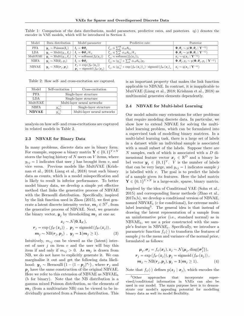
Table 1: Comparison of the data distributions, model parameters, predictive rates, and posteriors. q(·) denotes theencoder in VAE models, which will be introduced in Section 3.

Model Data distribution Model parameter Predictive rate Posterior

PFA yj ∼ Poisson(lj) lj = Φθj l′vj ∝∑Kk φvkθkj Φ,θj ∼ p(Φ,θj | Y−ij)

LDA yj ∼ Multi(y·j , lj) lj = Φθj/θ·j l′vj ∝∑Kk φvkθkj/θ·j Φ,θj ∼ p(Φ,θj | Y−ij)

MultiVAE yj ∼ Multi(y·j , lj) lj = softmax(fθ(zj)) l′vj ∝ softmax(fθ(zj))v zj ∼ q(zj | Y−ij)NBFA yj ∼ NB(lj , pj) lj = Φθj l′vj ∝ (y−ivj +

∑Kk φvkθkj)pj Φ,θj , pj ∼ p(Φ,θj , pj | Y−ij)

NBVAE yj ∼ NB(rj ,pj)rj = exp (fθr (zj))pj = sigmoid (fθp(zj)

l′vj ∝ (y−ivj + exp (fθr (zj))v) · sigmoid (fθp(zj)v zj ∼ q(zj | Y−ij)

Table 2: How self- and cross-excitation are captured.

Model Self-excitation Cross-excitation

PFA Single-layer structureLDA Single-layer structure

MultiVAE Multi-layer neural networks

NBFA y−ivj Single-layer structure

NBVAE y−ivj Multi-layer neural networks

analysis on how self- and cross-excitations are capturedin related models in Table 2.

2.3 NBVAE for Binary Data

In many problems, discrete data are in binary form.For example, suppose a binary matrix Y ∈ {0, 1}V×Nstores the buying history of N users on V items, whereyvj = 1 indicates that user j has brought item v, andvice versa. Previous models like MultiVAE (Krish-nan et al., 2018; Liang et al., 2018) treat such binarydata as counts, which is a model misspecification andis likely to result in inferior performance. To bettermodel binary data, we develop a simple yet effectivemethod that links the generative process of NBVAEwith the Bernoulli distribution. Specifically, inspiredby the link function used in Zhou (2015), we first gen-erate a latent discrete intensity vector, mj ∈ NV , fromthe generative process of NBVAE. Next, we generatethe binary vector, yj by thresholding mj at one as:

zj ∼ N (0, IK),

rj = exp (fθr (zj)) , pj = sigmoid (fθp(zj)) ,

mj ∼ NB(rj ,pj) , yj = 1(mj ≥ 1). (3)

Intuitively, mvj can be viewed as the (latent) inter-est of user j on item v and the user will buy thisitem if and only if mvj > 0. As mj is drawn fromNB, we do not have to explicitly generate it. We canmarginalise it out and get the following data likeli-hood: yj ∼ Bernoulli

(1− (1− pj)rj

), where rj and

pj have the same construction of the original NBVAE.Here we refer to this extension of NBVAE as NBVAEb

(b for binary). Note that the NB distribution is agamma mixed Poisson distribution, so the elements ofmj (from a multivariate NB) can be viewed to be in-dividually generated from a Poisson distribution. This

is an important property that makes the link functionapplicable to NBVAE. In contrast, it is inapplicable toMutiVAE (Liang et al., 2018; Krishnan et al., 2018) asmultinomial generates elements dependently.

2.4 NBVAE for Multi-label Learning

Our model admits easy extensions for other problemsthat require modeling discrete data. In particular, weshow how to extend NBVAE for solving the multi-label learning problem, which can be formulated intoa supervised task of modelling binary matrices. In amulti-label learning task, there is a large set of labelsin a dataset while an individual sample is associatedwith a small subset of the labels. Suppose there areN samples, each of which is associated with a D di-mensional feature vector xj ∈ RD and a binary la-bel vector yj ∈ {0, 1}V . V is the number of labelsthat can be very large, and yvj = 1 indicates sample jis labelled with v. The goal is to predict the labelsof a sample given its features. Here the label matrixY ∈ {0, 1}V×N is a large-scale, sparse, binary matrix.

Inspired by the idea of Conditional VAE (Sohn et al.,2015) and corresponding linear methods (Zhao et al.,2017a,b), we develop a conditional version of NBVAE,named NBVAEc (c for conditional), for extreme multi-label learning3. The general idea is that instead ofdrawing the latent representation of a sample froman uninformative prior (i.e., standard normal) as inNBVAEb, we use a prior constructed with the sam-ple’s feature in NBVAEc. Specifically, we introduce aparametric function fψ(·) to transform the features ofsample j to the mean and variance of the normal prior,formulated as follows:

µj ,σj = fψ(xj), zj ∼ N (µj ,diag{σ2j}),

rj = exp (fθr (zj)),pj = sigmoid (fθp(zj)) ,

mj ∼ NB(rj ,pj),yj = 1(mj ≥ 1). (4)

Note that fψ(·) defines p(zj | xj), which encodes the

3Other approaches that incorporate super-vised/conditional information in VAEs can also beused in our model. The main purpose here is to demon-strate our model’s appealing potential for modellingbinary data as well its model flexibility.


features of a sample into the prior of its latent repre-sentation. Intuitively, we name it the feature encoder.With the above construction, given the feature vectorof a testing sample j∗, we can feed xj∗ into the featureencoder to sample the latent representation, zj∗ , thenfeed it into the decoder to predict its labels.

3 VARIATIONAL INFERENCE

The inference of NBVAE and NBVAEb follows thestandard amortized variational inference procedure ofVAEs, where a data-dependent variational distribu-tion q(zj | yj) (i.e., encoder) is used to approximatethe true posterior, p(zj | yj), as follows:

µj , σj = fφ(yj), zj ∼ N (µj ,diag{σ2j}). (5)

Given q(zj | yj), the learning objective is to maximisethe Evidence Lower BOund (ELBO) of the marginallikelihood of the data: Eq(zj |yj)

[log p(yj | zj)

]−

KL[q(zj | yj) ‖ p(zj)

], in terms of the decoder pa-

rameters θr, θp and the encoder parameter φ. Here thereparametrization trick (Kingma and Welling, 2014;Rezende et al., 2014) is used to sample from q(zj | yj).

For NBVAEc, there are two differences of inferencefrom the above two models: 1) Due to the use of the in-formative prior conditioned on features, the Kullback-Leiber (KL) divergence on the RHS of the ELBO iscalculated between two non-standard multivariate nor-mal distributions: KL

[q(zj | yj) ‖ p(zj | xj)

]. Thus,

the KL divergence of the ELBO does not only serveas a regularizer for q(zj | yj) but also helps learn thefeature encoder, fψ(·). 2) In NBVAEc, the feature en-coder plays an important role, as it is the one thatgenerates the latent representations for test samples.To get more opportunities to train it, when samplingzj in the training phase, we propose to alternativelydraw it between zj ∼ q(zj | yj) and zj ∼ p(zj | xj).This enables the feature encoder to directly contributeto the generation of labels, which improves its perfor-mance in the testing phase.

4 RELATED WORK

Probabilistic matrix factorisation models fordiscrete data. Several well-known models fall intothis category, including LDA (Blei et al., 2003) andPFA (Zhou et al., 2012), as well as their hierarchi-cal extensions such as those in Blei et al. (2010);Teh et al. (2012); Paisley et al. (2015); Gan et al.(2015a); Ranganath et al. (2015); Henao et al. (2015);Lim et al. (2016); Zhou et al. (2016); Zhao et al.(2017b, 2018b). Among various models, the clos-est ones to ours are NBFA (Zhou, 2018) and non-parametric LDA (Buntine and Mishra, 2014), which

generate data with the negative-binomial distributionand Dirichlet-multinomial distribution, respectively.Our models can be viewed as a deep generative exten-sions to them, providing better model expressiveness,flexibility, as well as inference scalability.

VAEs for discrete data. Miao et al. (2016) pro-posed Neural Variational Document Model (NVDM),which extended the standard VAE with multinomiallikelihood for document modelling. Miao et al. (2017)further built a VAE to generate the document-topicdistributions in the LDA framework. Srivastava andSutton (2017) developed an AVI algorithm for the in-ference of LDA, which can be viewed as a VAE model.Card et al. (2018) introduced a general VAE frame-work for topic modelling with meta-data. Grønbechet al. (2019) recently proposed a Gaussian mixtureVAE with negative-binomial for gene-expression data,which has a different construction to ours and does notconsider binary data, multi-label learning, or in-depthanalysis. Burkhardt and Kramer (2019) proposed aVAE framework for topic modelling, the latent repre-sentations of which are drawn from Dirichlet insteadof Gaussian. Krishnan et al. (2018) found that us-ing the standard training algorithm of VAEs in largesparse discrete data may suffer from model underfit-ting and proposed a stochastic variational inference(SVI) (Hoffman et al., 2013) algorithm initialised byAVI to mitigate this issue. In the collaborative filteringdomain, Liang et al. (2018) noticed a similar issue andalleviated it by proposing MultiVAE with a trainingscheme based on KL annealing (Bowman et al., 2016).Note that NVDM, NFA, and MultiVAE are the closestones to ours, their generative processes are very simi-lar but their inference procedures are different. NFA isreported to outperform NVDM on text analysis (Kr-ishnan et al., 2018) while MultiVAE is reported to havebetter performance than NFA on collaborative filter-ing tasks (Liang et al., 2018). Compared with them,we improve the modelling performance in a differentway, i.e., by better capturing self- and cross-excitationsso as to better handle overdispersion. Moreover, NFAand MultiVAE use the multinomial likelihood, whichmay not work well for binary data.

VAEs for multi-label learning. In various applica-tions, such as image/document tagging, recommendersystem, ad-placement, multi-label learning/extremeclassification problems have drawn a significant atten-tion (Yu et al., 2014; Mencia and Furnkranz, 2008;Yen et al., 2016; Bhatia et al., 2015; Rai et al., 2015;Jain et al., 2016; Prabhu et al., 2018a; You et al., 2018;Prabhu et al., 2018b). Most of the existing state-of-the-art methods adopt either multiple steps of process-ing of the labels and features or complex optimisationalgorithms. In contrast, NBVAEc achieves compara-


ble performance but with much simpler model struc-tures. To our knowledge, the adaptation of VAEs tothe multi-label learning area is rare, because most ex-isting VAE models are unable to deal with large-scalesparse binary label matrices effectively.

5 EXPERIMENTS

In this section, we evaluate the proposed models onthree important applications of large-scale discretedata: text analysis, collaborative filtering, and multi-label learning. We run our models multiple times andreport the average results. The details of the datasets,evaluation metrics, experimental settings, and runningtime comparison are provided in the appendix.

5.1 Experiments on Text Analysis

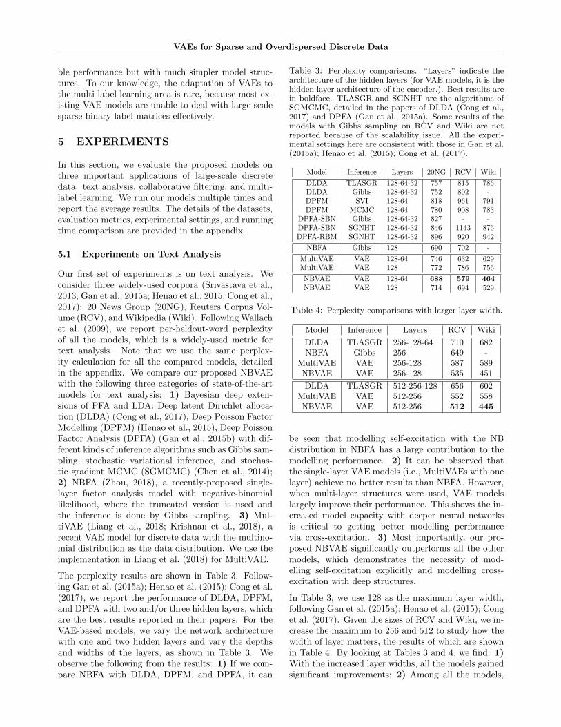
Our first set of experiments is on text analysis. Weconsider three widely-used corpora (Srivastava et al.,2013; Gan et al., 2015a; Henao et al., 2015; Cong et al.,2017): 20 News Group (20NG), Reuters Corpus Vol-ume (RCV), and Wikipedia (Wiki). Following Wallachet al. (2009), we report per-heldout-word perplexityof all the models, which is a widely-used metric fortext analysis. Note that we use the same perplex-ity calculation for all the compared models, detailedin the appendix. We compare our proposed NBVAEwith the following three categories of state-of-the-artmodels for text analysis: 1) Bayesian deep exten-sions of PFA and LDA: Deep latent Dirichlet alloca-tion (DLDA) (Cong et al., 2017), Deep Poisson FactorModelling (DPFM) (Henao et al., 2015), Deep PoissonFactor Analysis (DPFA) (Gan et al., 2015b) with dif-ferent kinds of inference algorithms such as Gibbs sam-pling, stochastic variational inference, and stochas-tic gradient MCMC (SGMCMC) (Chen et al., 2014);2) NBFA (Zhou, 2018), a recently-proposed single-layer factor analysis model with negative-binomiallikelihood, where the truncated version is used andthe inference is done by Gibbs sampling. 3) Mul-tiVAE (Liang et al., 2018; Krishnan et al., 2018), arecent VAE model for discrete data with the multino-mial distribution as the data distribution. We use theimplementation in Liang et al. (2018) for MultiVAE.

The perplexity results are shown in Table 3. Follow-ing Gan et al. (2015a); Henao et al. (2015); Cong et al.(2017), we report the performance of DLDA, DPFM,and DPFA with two and/or three hidden layers, whichare the best results reported in their papers. For theVAE-based models, we vary the network architecturewith one and two hidden layers and vary the depthsand widths of the layers, as shown in Table 3. Weobserve the following from the results: 1) If we com-pare NBFA with DLDA, DPFM, and DPFA, it can

Table 3: Perplexity comparisons. “Layers” indicate thearchitecture of the hidden layers (for VAE models, it is thehidden layer architecture of the encoder.). Best results arein boldface. TLASGR and SGNHT are the algorithms ofSGMCMC, detailed in the papers of DLDA (Cong et al.,2017) and DPFA (Gan et al., 2015a). Some results of themodels with Gibbs sampling on RCV and Wiki are notreported because of the scalability issue. All the experi-mental settings here are consistent with those in Gan et al.(2015a); Henao et al. (2015); Cong et al. (2017).

Model Inference Layers 20NG RCV Wiki

DLDA TLASGR 128-64-32 757 815 786DLDA Gibbs 128-64-32 752 802 -DPFM SVI 128-64 818 961 791DPFM MCMC 128-64 780 908 783

DPFA-SBN Gibbs 128-64-32 827 - -DPFA-SBN SGNHT 128-64-32 846 1143 876DPFA-RBM SGNHT 128-64-32 896 920 942

NBFA Gibbs 128 690 702 -

MultiVAE VAE 128-64 746 632 629MultiVAE VAE 128 772 786 756

NBVAE VAE 128-64 688 579 464NBVAE VAE 128 714 694 529

Table 4: Perplexity comparisons with larger layer width.

Model Inference Layers RCV Wiki

DLDA TLASGR 256-128-64 710 682NBFA Gibbs 256 649 -

MultiVAE VAE 256-128 587 589NBVAE VAE 256-128 535 451

DLDA TLASGR 512-256-128 656 602MultiVAE VAE 512-256 552 558NBVAE VAE 512-256 512 445

be seen that modelling self-excitation with the NBdistribution in NBFA has a large contribution to themodelling performance. 2) It can be observed thatthe single-layer VAE models (i.e., MultiVAEs with onelayer) achieve no better results than NBFA. However,when multi-layer structures were used, VAE modelslargely improve their performance. This shows the in-creased model capacity with deeper neural networksis critical to getting better modelling performancevia cross-excitation. 3) Most importantly, our pro-posed NBVAE significantly outperforms all the othermodels, which demonstrates the necessity of mod-elling self-excitation explicitly and modelling cross-excitation with deep structures.

In Table 3, we use 128 as the maximum layer width,following Gan et al. (2015a); Henao et al. (2015); Conget al. (2017). Given the sizes of RCV and Wiki, we in-crease the maximum to 256 and 512 to study how thewidth of layer matters, the results of which are shownin Table 4. By looking at Tables 3 and 4, we find: 1)With the increased layer widths, all the models gainedsignificant improvements; 2) Among all the models,


200 400 600 800 10000

1000

2000MultiVAE

200 400 600 800 10000

1000

2000NBFA

200 400 600 800 10000

1000

2000NBVAEdm

200 400 600 800 10000

1000

2000NBVAE

200 400 600 800 10000

1000

2000MultiVAE

200 400 600 800 10000

1000

2000NBFA

200 400 600 800 10000

1000

2000NBVAEdm

200 400 600 800 10000

1000

2000NBVAE

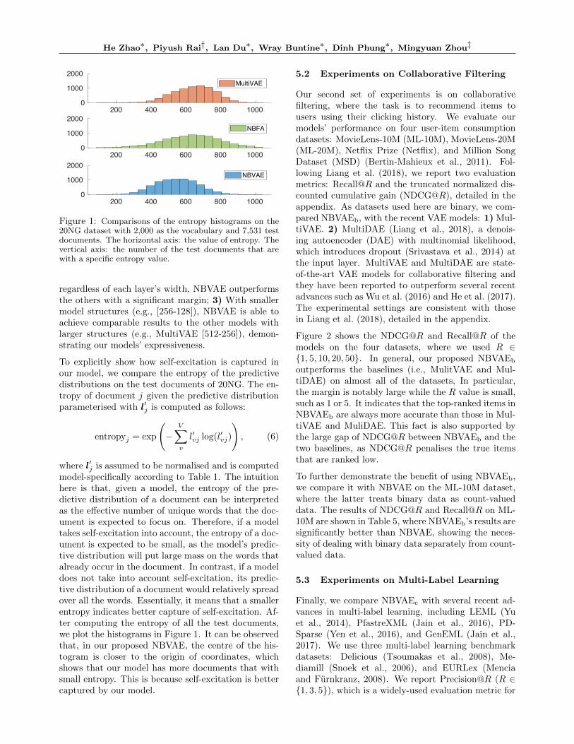
Figure 1: Comparisons of the entropy histograms on the20NG dataset with 2,000 as the vocabulary and 7,531 testdocuments. The horizontal axis: the value of entropy. Thevertical axis: the number of the test documents that arewith a specific entropy value.

regardless of each layer’s width, NBVAE outperformsthe others with a significant margin; 3) With smallermodel structures (e.g., [256-128]), NBVAE is able toachieve comparable results to the other models withlarger structures (e.g., MultiVAE [512-256]), demon-strating our models’ expressiveness.

To explicitly show how self-excitation is captured inour model, we compare the entropy of the predictivedistributions on the test documents of 20NG. The en-tropy of document j given the predictive distributionparameterised with l′j is computed as follows:

entropyj = exp

(−

V∑v

l′vj log(l′vj)

), (6)

where l′j is assumed to be normalised and is computedmodel-specifically according to Table 1. The intuitionhere is that, given a model, the entropy of the pre-dictive distribution of a document can be interpretedas the effective number of unique words that the doc-ument is expected to focus on. Therefore, if a modeltakes self-excitation into account, the entropy of a doc-ument is expected to be small, as the model’s predic-tive distribution will put large mass on the words thatalready occur in the document. In contrast, if a modeldoes not take into account self-excitation, its predic-tive distribution of a document would relatively spreadover all the words. Essentially, it means that a smallerentropy indicates better capture of self-excitation. Af-ter computing the entropy of all the test documents,we plot the histograms in Figure 1. It can be observedthat, in our proposed NBVAE, the centre of the his-togram is closer to the origin of coordinates, whichshows that our model has more documents that withsmall entropy. This is because self-excitation is bettercaptured by our model.

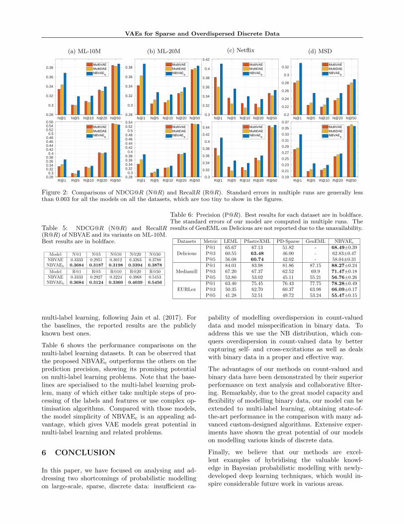
5.2 Experiments on Collaborative Filtering

Our second set of experiments is on collaborativefiltering, where the task is to recommend items tousers using their clicking history. We evaluate ourmodels’ performance on four user-item consumptiondatasets: MovieLens-10M (ML-10M), MovieLens-20M(ML-20M), Netflix Prize (Netflix), and Million SongDataset (MSD) (Bertin-Mahieux et al., 2011). Fol-lowing Liang et al. (2018), we report two evaluationmetrics: Recall@R and the truncated normalized dis-counted cumulative gain (NDCG@R), detailed in theappendix. As datasets used here are binary, we com-pared NBVAEb, with the recent VAE models: 1) Mul-tiVAE. 2) MultiDAE (Liang et al., 2018), a denois-ing autoencoder (DAE) with multinomial likelihood,which introduces dropout (Srivastava et al., 2014) atthe input layer. MultiVAE and MultiDAE are state-of-the-art VAE models for collaborative filtering andthey have been reported to outperform several recentadvances such as Wu et al. (2016) and He et al. (2017).The experimental settings are consistent with thosein Liang et al. (2018), detailed in the appendix.

Figure 2 shows the NDCG@R and Recall@R of themodels on the four datasets, where we used R ∈{1, 5, 10, 20, 50}. In general, our proposed NBVAEb

outperforms the baselines (i.e., MulitVAE and Mul-tiDAE) on almost all of the datasets, In particular,the margin is notably large while the R value is small,such as 1 or 5. It indicates that the top-ranked items inNBVAEb are always more accurate than those in Mul-tiVAE and MuliDAE. This fact is also supported bythe large gap of NDCG@R between NBVAEb and thetwo baselines, as NDCG@R penalises the true itemsthat are ranked low.

To further demonstrate the benefit of using NBVAEb,we compare it with NBVAE on the ML-10M dataset,where the latter treats binary data as count-valueddata. The results of NDCG@R and Recall@R on ML-10M are shown in Table 5, where NBVAEb’s results aresignificantly better than NBVAE, showing the neces-sity of dealing with binary data separately from count-valued data.

5.3 Experiments on Multi-Label Learning

Finally, we compare NBVAEc with several recent ad-vances in multi-label learning, including LEML (Yuet al., 2014), PfastreXML (Jain et al., 2016), PD-Sparse (Yen et al., 2016), and GenEML (Jain et al.,2017). We use three multi-label learning benchmarkdatasets: Delicious (Tsoumakas et al., 2008), Me-diamill (Snoek et al., 2006), and EURLex (Menciaand Furnkranz, 2008). We report Precision@R (R ∈{1, 3, 5}), which is a widely-used evaluation metric for


(a) ML-10M

N@1 N@5 N@10 N@20 [email protected]

0.3

0.32

0.34

0.36

0.38MultiVAEMultiDAENBVAE

b

(b) ML-20M


0.3

0.32

0.34

0.36


b

(c) Netflix


0.32

0.34

0.36

0.38

0.4


b

(d) MSD


0.22

0.24

0.26

0.28

0.3


b

R@1 R@5 R@10 R@20 [email protected]

0.30.320.340.360.38

0.40.420.440.460.48

0.50.520.540.56

MultiVAEMultiDAENBVAE

b


0.30.320.340.360.38

0.40.420.440.460.48

0.50.520.54

MultiVAEMultiDAENBVAE

b


0.32

0.34

0.36

0.38

0.4

0.42

0.44 MultiVAEMultiDAENBVAE

b


0.21

0.23

0.25

0.27

0.29

0.31

0.33

0.35


b

Figure 2: Comparisons of NDCG@R (N@R) and RecallR (R@R). Standard errors in multiple runs are generally lessthan 0.003 for all the models on all the datasets, which are too tiny to show in the figures.

Table 5: NDCG@R (N@R) and RecallR(R@R) of NBVAE and its variants on ML-10M.Best results are in boldface.

Model N@1 N@5 N@10 N@20 N@50NBVAE 0.3333 0.2951 0.3012 0.3263 0.3788NBVAEb 0.3684 0.3187 0.3198 0.3394 0.3878

Model R@1 R@5 R@10 R@20 R@50NBVAE 0.3333 0.2927 0.3224 0.3968 0.5453NBVAEb 0.3684 0.3124 0.3360 0.4039 0.5456

Table 6: Precision (P@R). Best results for each dataset are in boldface.The standard errors of our model are computed in multiple runs. Theresults of GenEML on Delicious are not reported due to the unavailability.

Datasets Metric LEML PfastreXML PD-Sparse GenEML NBVAEc

DeliciousP@1P@3P@5

65.6760.5556.08

67.1363.4860.74

51.8246.0042.02

---

68.49±0.3962.83±0.4758.04±0.31

MediamillP@1P@3P@5

84.0167.2052.80

83.9867.3753.02

81.8662.5245.11

87.1569.955.21

88.27±0.2471.47±0.1856.76±0.26

EURLexP@1P@3P@5

63.4050.3541.28

75.4562.7052.51

76.4360.3749.72

77.7563.9853.24

78.28±0.4966.09±0.1755.47±0.15

multi-label learning, following Jain et al. (2017). Forthe baselines, the reported results are the publiclyknown best ones.

Table 6 shows the performance comparisons on themulti-label learning datasets. It can be observed thatthe proposed NBVAEc outperforms the others on theprediction precision, showing its promising potentialon multi-label learning problems. Note that the base-lines are specialised to the multi-label learning prob-lem, many of which either take multiple steps of pro-cessing of the labels and features or use complex op-timisation algorithms. Compared with those models,the model simplicity of NBVAEc is an appealing ad-vantage, which gives VAE models great potential inmulti-label learning and related problems.

6 CONCLUSION

In this paper, we have focused on analysing and ad-dressing two shortcomings of probabilistic modellingon large-scale, sparse, discrete data: insufficient ca-

pability of modelling overdispersion in count-valueddata and model misspecification in binary data. Toaddress this we use the NB distribution, which con-quers overdispersion in count-valued data by bettercapturing self- and cross-excitations as well as dealswith binary data in a proper and effective way.

The advantages of our methods on count-valued andbinary data have been demonstrated by their superiorperformance on text analysis and collaborative filter-ing. Remarkably, due to the great model capacity andflexibility of modelling binary data, our model can beextended to multi-label learning, obtaining state-of-the-art performance in the comparison with many ad-vanced custom-designed algorithms. Extensive exper-iments have shown the great potential of our modelson modelling various kinds of discrete data.

Finally, we believe that our methods are excel-lent examples of hybridising the valuable knowl-edge in Bayesian probabilistic modelling with newly-developed deep learning techniques, which would in-spire considerable future work in various areas.


Acknowledgements: MZ was supported in part byNSF IIS-1812699. PR acknowledges support fromVisvesvaraya Young Faculty Fellowship. DP gratefullyacknowledges funding support from the Australian Re-search Council under the ARC DP160109394 Project.

References

T. Bertin-Mahieux, D. P. Ellis, B. Whitman, andP. Lamere. The million song dataset. In Interna-tional Conference on Music Information Retrieval,2011.

K. Bhatia, H. Jain, P. Kar, M. Varma, and P. Jain.Sparse local embeddings for extreme multi-labelclassification. In NIPS, pages 730–738, 2015.

D. M. Blei, A. Y. Ng, and M. I. Jordan. Latent Dirich-let allocation. JMLR, 3:993–1022, 2003.

D. M. Blei, T. L. Griffiths, and M. I. Jordan. Thenested Chinese restaurant process and Bayesiannonparametric inference of topic hierarchies. Jour-nal of the ACM, 57(2):7, 2010.

S. R. Bowman, L. Vilnis, O. Vinyals, A. Dai, R. Joze-fowicz, and S. Bengio. Generating sentences from acontinuous space. In CoNLL, pages 10–21, 2016.

W. L. Buntine and S. Mishra. Experiments with non-parametric topic models. In SIGKDD, pages 881–890, 2014.

S. Burkhardt and S. Kramer. Decoupling sparsity andsmoothness in the Dirichlet variational autoencodertopic model. JMLR, 20(131):1–27, 2019.

J. Canny. GaP: a factor model for discrete data. InSIGIR, pages 122–129, 2004.

D. Card, C. Tan, and N. A. Smith. Neural modelsfor documents with metadata. In ACL, pages 2031–2040, 2018.

T. Chen, E. Fox, and C. Guestrin. Stochastic gradientHamiltonian Monte Carlo. In ICML, pages 1683–1691, 2014.

K. W. Church and W. A. Gale. Poisson mixtures.Natural Language Engineering, 1(2):163–190, 1995.

Y. Cong, B. Chen, H. Liu, and M. Zhou. Deep la-tent Dirichlet allocation with topic-layer-adaptivestochastic gradient Riemannian MCMC. In ICML,pages 864–873, 2017.

G. Doyle and C. Elkan. Accounting for burstiness intopic models. In ICML, pages 281–288, 2009.

Z. Gan, C. Chen, R. Henao, D. Carlson, and L. Carin.Scalable deep Poisson factor analysis for topic mod-eling. In ICML, pages 1823–1832, 2015a.

Z. Gan, R. Henao, D. Carlson, and L. Carin. Learningdeep sigmoid belief networks with data augmenta-tion. In AISTATS, pages 268–276, 2015b.

C. H. Grønbech, M. F. Vording, P. N. Timshel, C. K.Sønderby, T. H. Pers, and O. Winther. scVAE: Vari-ational auto-encoders for single-cell gene expressiondata. bioRxiv, page 318295, 2019.

X. He, L. Liao, H. Zhang, L. Nie, X. Hu, and T.-S. Chua. Neural collaborative filtering. In WWW,pages 173–182, 2017.

R. Henao, Z. Gan, J. Lu, and L. Carin. Deep Poissonfactor modeling. In NIPS, pages 2800–2808, 2015.

M. D. Hoffman, D. M. Blei, C. Wang, and J. Paisley.Stochastic variational inference. JMLR, 14(1):1303–1347, 2013.

H. Jain, Y. Prabhu, and M. Varma. Extreme multi-label loss functions for recommendation, tagging,ranking & other missing label applications. In KDD,2016.

V. Jain, N. Modhe, and P. Rai. Scalable generativemodels for multi-label learning with missing labels.In ICML, pages 1636–1644, 2017.

D. P. Kingma and M. Welling. Auto-encoding varia-tional Bayes. In ICLR, 2014.

R. Krishnan, D. Liang, and M. Hoffman. On the chal-lenges of learning with inference networks on sparse,high-dimensional data. In AISTATS, pages 143–151,2018.

D. Liang, R. G. Krishncan, M. D. Hoffman, and T. Je-bara. Variational autoencoders for collaborative fil-tering. In WWW, pages 689–698, 2018.

K. W. Lim, W. Buntine, C. Chen, and L. Du. Non-parametric Bayesian topic modelling with the hier-archical Pitman-Yor processes. International Jour-nal of Approximate Reasoning, 78:172–191, 2016.

R. E. Madsen, D. Kauchak, and C. Elkan. Modelingword burstiness using the Dirichlet distribution. InICML, pages 545–552, 2005.

E. L. Mencia and J. Furnkranz. Efficient pairwise mul-tilabel classification for large-scale problems in thelegal domain. In ECML/PKDD, pages 50–65, 2008.

Y. Miao, L. Yu, and P. Blunsom. Neural variationalinference for text processing. In ICML, pages 1727–1736, 2016.

Y. Miao, E. Grefenstette, and P. Blunsom. Discov-ering discrete latent topics with neural variationalinference. In ICML, pages 2410–2419, 2017.

A. Mnih and R. R. Salakhutdinov. Probabilistic ma-trix factorization. In NIPS, pages 1257–1264, 2008.

J. Paisley, C. Wang, D. M. Blei, and M. I. Jordan.Nested hierarchical Dirichlet processes. TPAMI, 37(2):256–270, 2015.


Y. Prabhu, A. Kag, S. Gopinath, K. Dahiya, S. Har-sola, R. Agrawal, and M. Varma. Extreme multi-label learning with label features for warm-start tag-ging, ranking & recommendation. In WSDM, 2018a.

Y. Prabhu, A. Kag, S. Harsola, R. Agrawal, andM. Varma. Parabel: Partitioned label trees forextreme classification with application to dynamicsearch advertising. In WWW, 2018b.

P. Rai, C. Hu, R. Henao, and L. Carin. Large-scalebayesian multi-label learning via topic-based labelembeddings. In NIPS, 2015.

R. Ranganath, L. Tang, L. Charlin, and D. Blei. Deepexponential families. In AISTATS, pages 762–771,2015.

D. J. Rezende, S. Mohamed, and D. Wierstra. Stochas-tic backpropagation and approximate inference indeep generative models. In ICML, pages 1278–1286,2014.

C. G. Snoek, M. Worring, J. C. Van Gemert, J.-M.Geusebroek, and A. W. Smeulders. The challengeproblem for automated detection of 101 semanticconcepts in multimedia. In ACM MM, pages 421–430, 2006.

K. Sohn, H. Lee, and X. Yan. Learning structured out-put representation using deep conditional generativemodels. In NIPS, pages 3483–3491. 2015.

A. Srivastava and C. Sutton. Autoencoding variationalinference for topic models. In ICLR, 2017.

N. Srivastava, R. Salakhutdinov, and G. Hinton. Mod-eling documents with a deep Boltzmann machine. InUAI, pages 616–624, 2013.

N. Srivastava, G. Hinton, A. Krizhevsky, I. Sutskever,and R. Salakhutdinov. Dropout: a simple way toprevent neural networks from overfitting. JMLR, 15(1):1929–1958, 2014.

Y. Teh, M. Jordan, M. Beal, and D. Blei. HierarchicalDirichlet processes. Journal of the American Statis-tical Association, 101(476):1566–1581, 2012.

G. Tsoumakas, I. Katakis, and I. Vlahavas. Effec-tive and efficient multilabel classification in domainswith large number of labels. In ECML/PKDDWorkshop on Mining Multidimensional Data, vol-ume 21, pages 53–59, 2008.

H. M. Wallach, I. Murray, R. Salakhutdinov, andD. Mimno. Evaluation methods for topic models.In ICML, pages 1105–1112, 2009.

Y. Wu, C. DuBois, A. X. Zheng, and M. Ester. Col-laborative denoising auto-encoders for top-n recom-mender systems. In WSDM, pages 153–162, 2016.

I. E.-H. Yen, X. Huang, P. Ravikumar, K. Zhong, andI. Dhillon. PD-sparse: A primal and dual sparseapproach to extreme multiclass and multilabel clas-sification. In ICML, pages 3069–3077, 2016.

R. You, S. Dai, Z. Zhang, H. Mamitsuka, and S. Zhu.AttentionXML: Extreme multi-label text classifi-cation with multi-label attention based recurrentneural networks. arXiv preprint arXiv:1811.01727,2018.

H.-F. Yu, P. Jain, P. Kar, and I. Dhillon. Large-scalemulti-label learning with missing labels. In ICML,pages 593–601, 2014.

H. Zhao, L. Du, and W. Buntine. Leveraging nodeattributes for incomplete relational data. In ICML,pages 4072–4081, 2017a.

H. Zhao, L. Du, W. Buntine, and G. Liu. MetaLDA:A topic model that efficiently incorporates meta in-formation. In ICDM, pages 635–644, 2017b.

H. Zhao, L. Du, W. Buntine, and M. Zhou. Dirich-let belief networks for topic structure learning. InNeurIPS, pages 7966–7977, 2018a.

H. Zhao, L. Du, W. Buntine, and M. Zhou. Interand intra topic structure learning with word em-beddings. In ICML, pages 5887–5896, 2018b.

M. Zhou. Infinite edge partition models for overlap-ping community detection and link prediction. InAISTATS, pages 1135–1143, 2015.

M. Zhou. Nonparametric Bayesian negative binomialfactor analysis. Bayesian Analysis, 2018.

M. Zhou, L. Hannah, D. B. Dunson, and L. Carin.Beta-negative binomial process and Poisson factoranalysis. In AISTATS, pages 1462–1471, 2012.

M. Zhou, Y. Cong, and B. Chen. Augmentable gammabelief networks. JMLR, 17(163):1–44, 2016.

Variational Autoencoders for Sparse and Overdispersed ...

Documents

Transcript of Variational Autoencoders for Sparse and Overdispersed ...