mathematics

Article

R-Adaptive Multisymplectic and Variational Integrators

Tomasz M. Tyranowski 1,2,*,† and Mathieu Desbrun 2,†

1 Max-Planck-Institut für Plasmaphysik, Boltzmannstraße 2, 85748 Garching, Germany2 Department of Computing and Mathematical Sciences, California Institute of Technology, Pasadena,

CA 91125, USA* Correspondence: tomasz.tyranowski@ipp.mpg.de† These authors contributed equally to this work.

Received: 30 May 2019; Accepted: 9 July 2019; Published: 18 July 2019

Abstract: Moving mesh methods (also called r-adaptive methods) are space-adaptive strategies usedfor the numerical simulation of time-dependent partial differential equations. These methods keepthe total number of mesh points fixed during the simulation but redistribute them over time tofollow the areas where a higher mesh point density is required. There are a very limited numberof moving mesh methods designed for solving field-theoretic partial differential equations, and thenumerical analysis of the resulting schemes is challenging. In this paper, we present two ways toconstruct r-adaptive variational and multisymplectic integrators for (1+1)-dimensional Lagrangianfield theories. The first method uses a variational discretization of the physical equations, and themesh equations are then coupled in a way typical of the existing r-adaptive schemes. The secondmethod treats the mesh points as pseudo-particles and incorporates their dynamics directly intothe variational principle. A user-specified adaptation strategy is then enforced through Lagrangemultipliers as a constraint on the dynamics of both the physical field and the mesh points. We discussthe advantages and limitations of our methods. Numerical results for the Sine–Gordon equation arealso presented.

Keywords: geometric numerical integration; variational integrators; multisymplectic integrators;field theory; moving mesh methods; moving mesh partial differential equations; solitons;Sine–Gordon equation

1. Introduction

The purpose of this work is to design, analyze, and implement variational and multisymplecticintegrators for Lagrangian partial differential equations with space-adaptive meshes. In this paper, wecombine geometric numerical integration and r-adaptive methods for the numerical solution of PartialDifferential Equations (PDEs). We show that these two fields are compatible, mostly due to the factthat, in r-adaptation, the number of mesh points remains constant and we can treat them as additionalpseudo-particles of which the dynamics are coupled to the dynamics of the physical field of interest.

Geometric (or structure-preserving) integrators are numerical methods that preserve geometricproperties of the flow of a differential equation (see Reference [1]). This encompasses symplecticintegrators for Hamiltonian systems, variational integrators for Lagrangian systems, and numericalmethods on manifolds, including Lie group methods and integrators for constrained mechanicalsystems. Geometric integrators proved to be extremely useful for numerical computations inastronomy, molecular dynamics, mechanics, and theoretical physics. The main motivation fordeveloping structure-preserving algorithms lies in the fact that they show excellent numerical behavior,especially for long-time integration of equations possessing geometric properties.

An important class of structure-preserving integrators are variational integrators for Lagrangiansystems [1,2]. This type of integrator is based on discrete variational principles. The variational

Mathematics 2019, 7, 642; doi:10.3390/math7070642 www.mdpi.com/journal/mathematics

Mathematics 2019, 7, 642 2 of 52

approach provides a unified framework for the analysis of many symplectic algorithms and ischaracterized by a natural treatment of the discrete Noether theorem, as well as forced, dissipative, andconstrained systems. Variational integrators were first introduced in the context of finite-dimensionalmechanical systems, but later, Marsden, Patrick, and Shkoller [3] generalized this idea to field theories.Variational integrators have since been successfully applied in many computations, for example inelasticity [4], electrodynamics [5], or fluid dynamics [6]. Existing variational integrators so far havebeen developed on static, mostly uniform spatial meshes. The main goal of this paper is to design andanalyze variational integrators that allow for the use of space-adaptive meshes.

Adaptive meshes used for the numerical solution of partial differential equations fall into threemain categories: h-adaptive, p-adaptive, and r-adaptive. R-adaptive methods, which are also knownas moving mesh methods [7,8], keep the total number of mesh points fixed during the simulationbut relocate them over time. These methods are designed to minimize the error of the computations byoptimally distributing the mesh points, contrasting with h-adaptive methods for which the accuracy ofthe computations is obtained via insertion and deletion of mesh points. Moving mesh methods are alarge and interesting research field of applied mathematics, and their role in modern computationalmodeling is growing. Despite the increasing interest in these methods in recent years, they are still in arelatively early stage of their development compared to the more matured h-adaptive methods.

1.1. Overview

There are three logical steps to r-adaptation:

• Discretization of the physical PDE• Mesh adaptation strategy• Coupling the mesh equations to the physical equations

The key ideas of this paper regard the first and the last step. Following the general spiritof variational integrators, we discretize the underlying action functional rather than the PDEitself and then derive the discrete equations of motion. We base our adaptation strategies on theequidistribution principle and the resulting moving mesh partial differential equations (MMPDEs).We interpret MMPDEs as constraints, which allows us to consider novel ways of coupling them to thephysical equations. Note that we will restrict our explanations to one time and one space dimensionfor the sake of simplicity.

Let us consider a (1+1)-dimensional scalar field theory with the action functional

S[φ] =∫ Tmax

0

∫ Xmax

0L(φ, φX , φt) dX dt, (1)

where φ : [0, Xmax]× [0, Tmax] −→ R is the field and L : R× R× R −→ R its Lagrangian density.For simplicity, we assume the following fixed boundary conditions

φ(0, t) = φL,

φ(Xmax, t) = φR. (2)

In order to further consider moving meshes let us perform a change of variables X = X(x, t)such that for all t the map X(., t) : [0, Xmax] −→ [0, Xmax] is a “diffeomorphism”—more precisely,we only require that X(., t) is a homeomorphism such that both X(., t) and X(., t)−1 are piecewiseC1. In the context of mesh adaptation, the map X(x, t) represents the spatial position at time t ofthe mesh point labeled by x. Define ϕ(x, t) = φ(X(x, t), t). Then, the partial derivatives of φ areφX(X(x, t), t) = ϕx/Xx and φt(X(x, t), t) = ϕt − ϕxXt/Xx. Plugging these equations in Equation (1),we get

S[φ] =∫ Tmax

0

∫ Xmax

0L(

ϕ,ϕx

Xx, ϕt −

ϕxXt

Xx

)Xx dx dt =: S[ϕ], S[ϕ, X] (3)

Mathematics 2019, 7, 642 3 of 52

where the last equality defines two modified, or “reparametrized”, action functionals. For the first one,S is considered as a functional of ϕ only, whereas in the second one we also treat it as a functional of X.This leads to two different approaches to mesh adaptation, which we dub the control-theoretic strategyand the Lagrange multiplier strategy, respectively. The “reparametrized” field theories defined by S[ϕ]and S[ϕ, X] are both intrinsically covariant; however, it is convenient for computational purposes towork with a space-time split and to formulate the field dynamics as an initial value problem.

1.2. Outline

This paper is organized as follows. In Sections 2 and 3 we take the view of infinite dimensionalmanifolds of fields as configuration spaces and develop the control-theoretic and Lagrange multiplierstrategies in that setting. It allows us to discretize our system in space first and consider timediscretization later on. It is clear from our exposition that the resulting integrators are variational.In Section 4, we show how similar integrators can be constructed using the covariant formalism ofmultisymplectic field theory. We also show how the integrators from the previous sections can beinterpreted as multisymplectic. In Section 5, we apply our integrators to the Sine–Gordon equation andwe present our numerical results. We summarize our work in Section 6 and discuss several directionsin which it can be extended.

2. Control-Theoretic Approach to r-Adaptation

At first glance, it appears that the simplest and most straightforward way to construct anr-adaptive variational integrator would be to discretize the physical system in a similar mannerto the general approach to variational integration, i.e., discretize the underlying variational principle,then derive the mesh equations, and couple them to the physical equations in a way typical of theexisting r-adaptive algorithms. We explore this idea in this section and show that it indeed leads tospace adaptive integrators that are variational in nature. However, we also show that those integratorsdo not exhibit the behavior expected of geometric integrators, such as good energy conservation.We will refer to this strategy as control-theoretic, since, in this description, the field ϕ represents thephysical state of the system, while X can be interpreted as a control variable and the mesh equationscan be interpreted as feedback (see, e.g., Reference [9]).

2.1. Reparametrized Lagrangian

For the moment, let us assume that X(x, t) is a known function. We denote by ξ(X, t) the functionsuch that ξ(., t) = X(., t)−1, that is ξ(X(x, t), t) = x (We allow a little abuse of notation here: X denotesboth the argument of ξ and the change of variables X(x, t). If we wanted to be more precise, we wouldwrite X = h(x, t).). We thus have S[ϕ] = S[ϕ(ξ(X, t), t)].

Proposition 1. Extremizing S[φ] with respect to φ is equivalent to extremizing S[ϕ] with respect to ϕ.

Proof. The variational derivatives of S and S are related by the formula

δS[ϕ] · δϕ(x, t) = δS[ϕ(ξ(X, t), t)] · δϕ(ξ(X, t), t). (4)

Suppose φ(X, t) extremizes S[φ], i.e., δS[φ] · δφ = 0 for all variations δφ. Given the functionX(x, t), define ϕ(x, t) = φ(X(x, t), t). Then, by the formula above, we have δS[ϕ] = 0, so ϕ extremizesS. Conversely, suppose ϕ(x, t) extremizes S, that is δS[ϕ] · δϕ = 0 for all variations δϕ. Since we assumeX(., t) is a homeomorphism, we can define φ(X, t) = ϕ(ξ(X, t), t). Note that an arbitrary variationδφ(X, t) induces the variation δϕ(x, t) = δφ(X(x, t), t). Then, we have δS[φ] · δφ = δS[ϕ] · δϕ = 0 forall variations δφ, so φ(X, t) extremizes S[φ].

Mathematics 2019, 7, 642 4 of 52

The corresponding instantaneous Lagrangian L : Q×W ×R −→ R is

L[ϕ, ϕt, t] =∫ Xmax

0L(ϕ, ϕx, ϕt, t) dx (5)

with the Lagrangian density

L(ϕ, ϕx, ϕt, x, t) = L(

ϕ,ϕx

Xx, ϕt −

ϕxXt

Xx

)Xx. (6)

The function spaces Q and W must be chosen appropriately for the problem at hand so that theLagrangian in Equation (5) makes sense. For instance, for a free field, we will have Q = H1([0, Xmax])

and W = L2([0, Xmax]). Since X(x, t) is a function of t, we are looking at a time-dependent system.Even though the energy associated with the Lagrangian in Equation (5) is not conserved, the energy ofthe original theory associated with the action functional in Equation (1)

E =∫ Xmax

0

(φt

∂L∂φt

(φ, φX , φt)−L(φ, φX , φt))

dX (7)

=∫ Xmax

0

[(ϕt −

ϕxXt

Xx

) ∂L∂φt

(ϕ,

ϕx

Xx, ϕt −

ϕxXt

Xx

)−L

(ϕ,

ϕx

Xx, ϕt −

ϕxXt

Xx

)]Xx dx (8)

is conserved. To see this, note that if φ(X, t) extremizes S[φ], then dE/dt = 0 (computed fromEquation (7)). Trivially, this means that dE/dt = 0 when Equation (8) is invoked as well. Moreover,as we have noted earlier, φ(X, t) extremizes S[φ] iff ϕ(x, t) extremizes S[ϕ]. This means that the energy(Equation (8)) is constant on solutions of the reparametrized theory.

2.2. Spatial Finite Element Discretization

We begin with a discretization of the spatial dimension only, thus turning the originalinfinite-dimensional problem into a time-continuous finite-dimensional Lagrangian system.Let ∆x = Xmax/(N + 1), and define the reference uniform mesh xi = i · ∆x for i = 0, 1, ..., N + 1and the corresponding piecewise linear finite elements

ηi(x) =

x−xi−1

∆x , if xi−1 ≤ x ≤ xi,− x−xi+1

∆x , if xi ≤ x ≤ xi+1,0, otherwise.

(9)

We now restrict X(x, t) to be of the form

X(x, t) =N+1

∑i=0

Xi(t)ηi(x) (10)

with X0(t) = 0, XN+1(t) = Xmax, and arbitrary Xi(t), i = 1, 2, ..., N as long as X(., t) is ahomeomorphism for all t. In our context of numerical computations, the functions Xi(t) represent thecurrent position of the ith mesh point. Define the finite element spaces

QN = WN = span(η0, ..., ηN+1) (11)

and assume that QN ⊂ Q, WN ⊂W. Let us denote a generic element of QN by ϕ and a generic elementof WN by ϕ. We have the decompositions

ϕ(x) =N+1

∑i=0

yiηi(x), ϕ(x) =N+1

∑i=0

yiηi(x). (12)

Mathematics 2019, 7, 642 5 of 52

The numbers (yi, yi) thus form natural (global) coordinates on QN × WN . We can nowapproximate the dynamics of the system described by Equation (5) in the finite-dimensional spaceQN ×WN . Let us consider the restriction LN = L|QN×WN×R of the Lagrangian of Equation (5) toQN ×WN ×R. In the chosen coordinates, we have

LN(y0, ..., yN+1, y0, ..., yN+1, t) = L[ N+1

∑i=0

yiηi(x),N+1

∑i=0

yiηi(x), t]. (13)

Note that, given the boundary conditions (Equation (2)), y0, yN+1, y0, and yN+1 are fixed. We willthus no longer write them as arguments of LN .

The advantage of using a finite element discretization lies in the fact that the symplectic structureinduced on QN ×WN by LN is strictly a restriction (i.e., a pull-back) of the (pre-)symplectic structure(In most cases, the symplectic structure of (Q×W, L) is only weakly nondegenerate; see Reference [10])on Q×W. This establishes a direct link between symplectic integration of the finite-dimensionalmechanical system (QN ×WN , LN) and the infinite-dimensional field theory (Q×W, L).

2.3. Differential-Algebraic Formulation and Time Integration

We now consider time integration of the Lagrangian system (QN ×WN , LN). If the functionsXi(t) are known, then one can perform variational integration in the standard way, that is, define thediscrete Lagrangian Ld : R×QN ×R×QN → R and solve the corresponding discrete Euler–Lagrangeequations (see References [1,2]). Let tn = n · ∆t for n = 0, 1, 2, . . . be an increasing sequence of timesand y0, y1, . . . be the corresponding discrete path of the system in QN . The discrete Lagrangian Ld isan approximation to the exact discrete Lagrangian LE

d , such that

Ld(tn, yn, tn+1, yn+1) ≈ LEd (tn, yn, tn+1, yn+1) ≡

∫ tn+1

tnLN(y(t), y(t), t) dt, (14)

where yn = (yn1 , ..., yn

N), yn+1 = (yn+11 , ..., yn+1

N ), and y(t) are the solutions of the Euler–Lagrangeequations corresponding to LN with boundary values y(tn) = yn and y(tn+1) = yn+1. Dependingon the quadrature we use to approximate the integral in Equation (14), we obtain different typesof variational integrators. As will be discussed below, in r-adaptation, one has to deal with stiffdifferential equations or differential-algebraic equations; therefore, higher order implicit integrationin time is advisable (see References [11,12]). We will employ variational partitioned Runge–Kuttamethods. An s-stage Runge–Kutta method is constructed by choosing

Ld(tn, yn, tn+1, yn+1) = (tn+1 − tn)s

∑i=1

bi LN(Yi, Yi, ti), (15)

where ti = tn + ci(tn+1 − tn); the right-hand side is extremized under the constraintyn+1 = yn + (tn+1 − tn)∑s

i=1 biYi; and the internal stage variables Yi and Yi are related byYi = yn + (tn+1 − tn)∑s

j=1 aijYj. It can be shown that the variational integrator with the discreteLagrangian defined by Equation (15) is equivalent to an appropriately chosen symplectic partitionedRunge–Kutta method applied to the Hamiltonian system corresponding to LN (see Reference [1,2]).With this in mind, we turn our semi-discrete Lagrangian system (QN ×WN , LN) into the Hamiltoniansystem (QN ×W∗N , HN) via the standard Legendre transform

HN(y1, ..., yN , p1, ..., pN ; X1, ..., XN , X1, ..., XN) =N

∑i=1

pi yi − LN(y1, ..., yN , y1, ..., yN , t), (16)

where pi = ∂LN/∂yi and we explicitly stated the dependence on the positions Xi and velocities Xi ofthe mesh points. The Hamiltonian equations take the form (It is computationally more convenient

Mathematics 2019, 7, 642 6 of 52

to directly integrate the implicit Hamiltonian system pi = ∂LN/∂yi, pi = ∂LN/∂yi, but as long as thesystem described by Equation (1) is at least weakly nondegenerate, there is no theoretical issue withpassing to the Hamiltonian formulation, which we do for the clarity of our exposition.)

yi =∂HN∂pi

(y, p; X(t), X(t)

),

pi = −∂HN∂yi

(y, p; X(t), X(t)

).

(17)

Suppose that the function Xi(t) is C1 and that HN is smooth as a function of the yi’s, pi’s, Xi’s,and Xi’s (note that these assumptions are used for simplicity and can be easily relaxed, if necessary,depending on the regularity of the considered Lagrangian system). Then, the assumptions of Picard’stheorem are satisfied and there exists a unique C1 flow Ft0,t = (Fy

t0,t, Fpt0,t) : QN ×W∗N → QN ×W∗N for

Equation (17). This flow is symplectic.However, in practice, we do not know the Xi’s and we in fact would like to be able to adjust them

“on the fly”, based on the current behavior of the system. We will do that by introducing additionalconstraint functions gi(y1, ..., yN , X1, ..., XN) and demanding that the conditions gi = 0 be satisfied atall times (In the context of Control Theory, the constraints gi = 0 are called strict static state feedback.See Reference [9].). The choice of these functions will be discussed in Section 2.4. This leads to thefollowing system of differential-algebraic equations (DAEs) of index 1 (see References [11–13])

yi =∂HN∂pi

(y, p; X, X

),

pi = −∂HN∂yi

(y, p; X, X

),

0 = gi(y, X),

yi(t0) = y(0)i ,

pi(t0) = p(0)i

(18)

for i = 1, ..., N. Note that an initial condition for X is fixed by the constraints. This system is of index 1because one has to differentiate the algebraic equations with respect to time once in order to reduce itto an implicit system of ordinary differential equations (ODEs). In fact, the implicit system will takethe form

y =∂HN∂p

(y, p; X, X

),

p = −∂HN∂y

(y, p; X, X

),

0 =∂g∂y

(y, X)y +∂g∂X

(y, X)X,

y(t0) = y(0),

p(t0) = p(0),

X(t0) = X(0),

(19)

where X(0) is a vector of arbitrary initial condition for the Xi’s. Suppose again that HN is a smoothfunction of y, p, X, and X. Futhermore, suppose that g is a C1 function of y and X and that ∂g

∂X −∂g∂y

∂2 HN∂X∂p is invertible with its inverse bounded in a neighborhood of the exact solution. (Again, these

assumptions can be relaxed if necessary.) Then, by the Implicit Function Theorem, Equation (19) canbe solved explicitly for y, p, and X and the resulting explicit ODE system will satisfy the assumptions

Mathematics 2019, 7, 642 7 of 52

of Picard’s theorem. Let (y(t), p(t), X(t)) be the unique C1 solution to this ODE system (and hence toEquation (19)). We have the trivial result

Proposition 2. If g(y(0), X(0)) = 0, then (y(t), p(t), X(t)) is a solution to Equation (18). (Note thatthere might be other solutions, as for any given y(0), there might be more than one X(0) that solves theconstraint equations.)

In practice, we would like to integrate Equation (18). A question arises in what sense is the systemdefined by this equation symplectic and in what sense a numerical integration scheme for this systemcan be regarded as variational. Let us address these issues.

Proposition 3. Let (y(t), p(t), X(t)) be a solution to Equation (18) and use this X(t) to form the Hamiltoniansystem (17). Then, we have

y(t) = Fyt0,t(y

(0), p(0)), p(t) = Fpt0,t(y

(0), p(0))

andg(

Fyt0,t(y

(0), p(0)), X(t))= 0,

where Ft0,t(y, p) is the symplectic flow for Equation (17).

Proof. Note that the first two equations of Equation (18) are the same as Equation (17); therefore(y(t), p(t)) trivially satisfies Equation (17) with the initial conditions y(t0) = y(0) and p(t0) = p(0).Since the flow map Ft0,t is unique, we must have y(t) = Fy

t0,t(y(0), p(0)) and p(t) = Fp

t0,t(y(0), p(0)).

Then, we also must have g(

Fyt0,t(y

(0), p(0)), X(t))= 0, that is, the constraints are satisfied along one

particular integral curve of Equation (17) that passes through (y(0), p(0)) at t0.

Suppose we now would like to find a numerical approximation of the solution to Equation (17)using an s-stage partitioned Runge–Kutta method with coefficients aij, bi, aij, bi, and ci [1,14].The numerical scheme will take the form

Yi =∂HN∂p

(Yi, Pi; X(tn + ci∆t), X(tn + ci∆t)

),

Pi = −∂HN∂y

(Yi, Pi; X(tn + ci∆t), X(tn + ci∆t)

),

Yi = yn + ∆ts

∑j=1

aijY j,

Pi = pn + ∆ts

∑j=1

aij Pj,

yn+1 = yn + ∆ts

∑i=1

biYi,

pn+1 = pn + ∆ts

∑i=1

bi Pi,

(20)

where Yi, Yi, Pi, and Pi are the internal stages and ∆t is the integration timestep. Let us apply the samepartitioned Runge–Kutta method to Equation (18). In order to compute the internal stages Qi, Qi ofthe X variable, we use the state–space form approach, that is, we demand that the constraints and their

Mathematics 2019, 7, 642 8 of 52

time derivatives be satisfied (see Reference [12]). The new step value Xn+1 is computed by solving theconstraints as well. The resulting numerical scheme is thus

Yi =∂HN∂p

(Yi, Pi; Qi, Qi

),

Pi = −∂HN∂y

(Yi, Pi; Qi, Qi

),

Yi = yn + ∆ts

∑j=1

aijY j,

Pi = pn + ∆ts

∑j=1

aij Pj,

0 = g(Yi, Qi),

0 =∂g∂y

(Yi, Qi) Yi +∂g∂X

(Yi, Qi) Qi,

yn+1 = yn + ∆ts

∑i=1

biYi,

pn+1 = pn + ∆ts

∑i=1

bi Pi,

0 = g(yn+1, Xn+1).

(21)

We have the following trivial observation.

Proposition 4. If X(t) is defined to be a C1 interpolation of the internal stages Qi, Qi at times tn + ci∆t(that is, if the values X(tn + ci∆t) and X(tn + ci∆t) coincide with Qi and Qi), then the schemes defined byEquations (20) and (21) give the same numerical approximations yn and pn to the exact solution y(t) and p(t).

Intuitively, Proposition 4 states that we can apply a symplectic partitioned Runge–Kutta methodto the DAE system in Equation (18), which solves both for X(t) and (y(t), p(t)), and the result will bethe same as if we performed a symplectic integration of the Hamiltonian system in Equation (17) for(y(t), p(t)) with a known X(t).

2.4. Moving Mesh Partial Differential Equations

The concept of equidistribution is the most popular paradigm of r-adaptation (see References [7,8]).Given a continuous mesh density function ρ(X), the equidistribution principle seeks to find a mesh0 = X0 < X1 < ... < XN+1 = Xmax such that the following holds

∫ X1

0ρ(X) dX =

∫ X2

X1

ρ(X) dX = ... =∫ Xmax

XN

ρ(X) dX, (22)

that is, the quantity represented by the density function is equidistributed among all cells. In thecontinuous setting, we will say that the reparametrization X = X(x) equidistributes ρ(X) if

∫ X(x)

0ρ(X) dX =

xXmax

σ, (23)

where σ =∫ Xmax

0 ρ(X) dX is the total amount of the equidistributed quantity. Differentiate this equationwith respect to x to obtain

ρ(X(x))∂X∂x

=1

Xmaxσ. (24)

Mathematics 2019, 7, 642 9 of 52

It is still a global condition in the sense that σ has to be known. For computational purposes, it isconvenient to differentiate this relation again and to consider the following partial differential equation

∂

∂x

(ρ(X(x))

∂X∂x

)= 0 (25)

with the boundary conditions X(0) = 0, X(Xmax) = Xmax. The choice of the mesh density functionρ(X) is typically problem-dependent and the subject of much research. A popular example is thegeneralized solution arclength given by

ρ =

√1 + α2

( ∂φ

∂X

)2=

√1 + α2

( ϕx

Xx

)2. (26)

It is often used to construct meshes that can follow moving fronts with locally high gradients [7,8].With this choice, Equation (25) is equivalent to

α2 ϕx ϕxx + XxXxx = 0, (27)

assuming Xx > 0, which we demand anyway. A finite difference discretization on the mesh xi = i · ∆xgives us the set of constraints

gi(y1, ..., yN ,X1, ..., XN) =

α2(yi+1 − yi)2 + (Xi+1 − Xi)

2 − α2(yi − yi−1)2 − (Xi − Xi−1)

2 = 0,(28)

with the previously defined yi’s and Xi’s. This set of constraints can be used in Equation (18).

2.5. Example

To illustrate these ideas, let us consider the Lagrangian density

L(φ, φX , φt) =12

φ2t −W(φX). (29)

The reparametrized Lagrangian in Equation (5) takes the form

L[ϕ, ϕt, t] =∫ Xmax

0

[12

Xx

(ϕt −

ϕx

XxXt

)2−W

( ϕx

Xx

)Xx

]dx. (30)

Let N = 1 and φL = φR = 0. Then

ϕ(x, t) = y1(t)η1(x), X(x, t) = X1(t)η1(x) + Xmax η2(x). (31)

The semi-discrete Lagrangian is

LN(y1, y1, t) =X1(t)

6

(y1 −

y1

X1(t)X1(t)

)2

+Xmax − X1(t)

6

(y1 +

y1

Xmax − X1(t)X1(t)

)2

−W(

y1

X1(t)

)X1(t)−W

(− y1

Xmax − X1(t)

)(Xmax − X1(t)

).

(32)

Mathematics 2019, 7, 642 10 of 52

The Legendre transform gives p1 = ∂LN/∂y1 = Xmax y1/3; hence, the semi-discreteHamiltonian is

HN(y1, p1; X1, X1) =3

2Xmaxp2

1 −16

XmaxX21

X1(Xmax − X1)y2

1

+ W( y1

X1

)X1 + W

(− y1

Xmax − X1

)(Xmax − X1).

(33)

The corresponding DAE system is

y1 =3

Xmaxp1,

p1 =13

XmaxX21

X1(Xmax − X1)y1 −W ′

( y1

X1

)+ W ′

(− y1

Xmax − X1

),

0 = g1(y1, X1).

(34)

This system is to be solved for the unknown functions y1(t), p1(t), and X1(t). It is of index 1because we have three unknown functions and only two differential equations—the algebraic equationhas to be differentiated once in order to obtain a missing ODE.

2.6. Backward Error Analysis

The true power of symplectic integration of Hamiltonian equations is revealed through backwarderror analysis: It can be shown that a symplectic integrator for a Hamiltonian system with theHamiltonian H(q, p) defines the exact flow for a nearby Hamiltonian system, of which the Hamiltoniancan be expressed as the asymptotic series

H (q, p) = H(q, p) + ∆tH2(q, p) + ∆t2H3(q, p) + . . . (35)

Owing to this fact, under some additional assumptions, symplectic numerical schemes nearlyconserve the original Hamiltonian H(q, p) over exponentially long time intervals. See Reference [1]for details.

Let us briefly review the results of backward error analysis for the integrator defined byEquation (21). Suppose g(y, X) satisfies the assumptions of the Implicit Function Theorem. Then,at least locally, we can solve the constraint X = h(y). The Hamiltonian DAE system in Equation (18)can be then written as the following (implicit) ODE system for y and p

y =∂HN∂p

(y, p; h(y), h′(y)y

), (36)

p = −∂HN∂y

(y, p; h(y), h′(y)y

).

Since we used the state–space formulation, the numerical scheme of Equation (21) is equivalent toapplying the same partitioned Runge–Kutta method to Equations (36), that is, we have Qi = h(Yi) andQi = h′(Yi)Yi. We computed the corresponding modified equation for several symplectic methods,namely Gauss and Lobatto IIIA–IIIB quadratures. Unfortunately, none of the quadratures resulted ina form akin to Equation (36) for some modified Hamiltonian function HN related to HN by a seriessimilar to Equation (35). This hints at the fact that we should not expect this integrator to showexcellent energy conservation over long integration times. One could also consider the implicit ODEsystem of Equation (19), which has an obvious triple partitioned structure and could apply a differentRunge–Kutta method to each variable y, p, and X. Although we did not pursue this idea further,it seems unlikely it would bring a desirable result.

Mathematics 2019, 7, 642 11 of 52

We therefore conclude that the control-theoretic strategy, while yielding a perfectly legitimatenumerical method, does not take the full advantage of the underlying geometric structures. Let us pointout that, while we used a variational discretization of the governing physical PDE, the mesh equationswere coupled in a manner that is typical of the existing r-adaptive methods (see References [7,8]).We now turn our attention to a second approach, which offers a novel way of coupling the meshequations to the physical equations.

3. Lagrange Multiplier Approach to r-Adaptation

As we saw in Section 2, discretization of the variational principle alone is not sufficient if wewould like to accurately capture the geometric properties of the physical system described by the actionfunctional in Equation (1). In this section, we propose a new technique of coupling the mesh equationsto the physical equations. Our idea is based on the observation that, in r-adaptation, the number ofmesh points is constant; therefore, we can treat them as pseudo-particles and we can incorporate theirdynamics into the variational principle. We show that this strategy results in integrators that muchbetter preserve the energy of the considered system.

3.1. Reparametrized Lagrangian

In this approach, we treat X(x, t) as an independent field, that is, another degree of freedom,and we will treat the “modified” action defined by Equation (3) as a functional of both ϕ and X:S = S[ϕ, X]. For the purpose of the derivations below, we assume that ϕ(., t) and X(., t) are continuousand piecewise C1. One could consider the closure of this space in the topology of either the Hilbert orBanach spaces of sufficiently integrable functions and interpret differentiation in a sufficiently weaksense, but this functional-analytic aspect is of little importance for the developments in this section.We refer the interested reader to References [15,16]. As in Section 2.1, let ξ(X, t) be the function suchthat ξ(., t) = X(., t)−1, that is ξ(X(x, t), t) = x. Then, S[ϕ, X] = S[ϕ(ξ(X, t), t)]. We begin with twopropositions and one corollary which will be important for the rest of our exposition.

Proposition 5. Extremizing S[φ] with respect to φ is equivalent to extremizing S[ϕ, X] with respect to both ϕ

and X.

Proof. The variational derivatives of S and S are related by the formula

δ1S[ϕ, X] · δϕ(x, t) = δS[ϕ(ξ(X, t), t)] · δϕ(ξ(X, t), t),

δ2S[ϕ, X] · δX(x, t) = δS[ϕ(ξ(X, t), t)] ·(− ϕx(ξ(X, t), t)

Xx(ξ(X, t), t)δX(ξ(X, t), t)

),

(37)

where δ1 and δ2 denote differentiation with respect to the first and second arguments, respectively.Suppose φ(X, t) extremizes S[φ], i.e., δS[φ] · δφ = 0 for all variations δφ. Choose an arbitraryX(x, t) such that X(., t) is a (sufficiently smooth) homeomorphism, and define ϕ(x, t) = φ(X(x, t), t).Then, by the formula above, we have δ1S[ϕ, X] = 0 and δ2S[ϕ, X] = 0, so the pair (ϕ, X)

extremizes S. Conversely, suppose the pair (ϕ, X) extremizes S, that is δ1S[ϕ, X] · δϕ = 0 andδ2S[ϕ, X] · δX = 0 for all variations δϕ and δX. Since we assume X(., t) is a homeomorphism,we can define φ(X, t) = ϕ(ξ(X, t), t). Note that an arbitrary variation δφ(X, t) induces the variationδϕ(x, t) = δφ(X(x, t), t). Then, we have δS[φ] · δφ = δ1S[ϕ, X] · δϕ = 0 for all variations δφ, so φ(X, t)extremizes S[φ].

Proposition 6. The equation δ2S[ϕ, X] = 0 is implied by the equation δ1S[ϕ, X] = 0.

Proof. As we saw in the proof of Proposition 5, the condition δ1S[ϕ, X] · δϕ = 0 implies δS = 0.By Equation (37), this in turn implies δ2S[ϕ, X] · δX = 0 for all δX. Note that this argument cannot bereversed: δ2S[ϕ, X] · δX = 0 does not imply δS = 0 when ϕx = 0.

Mathematics 2019, 7, 642 12 of 52

Corollary 1. The field theory described by S[ϕ, X] is degenerate, and the solutions to the Euler–Lagrangeequations are not unique.

3.2. Spatial Finite Element Discretization

The Lagrangian of the “reparametrized” theory L : Q× G×W × Z −→ R,

L[ϕ, X, ϕt, Xt] =∫ Xmax

0L(

ϕ,ϕx

Xx, ϕt −

ϕxXt

Xx

)Xx dx, (38)

has the same form as in Equation (5) (we only treat it as a functional of X and Xt as well), where Q,G, W, and Z are spaces of continuous and piecewise C1 functions, as mentioned before. We again let∆x = Xmax/(N + 1) and define the uniform mesh xi = i · ∆x for i = 0, 1, ..., N + 1. Define the finiteelement spaces

QN = GN = WN = ZN = span(η0, ..., ηN+1), (39)

where we used the finite elements introduced in Equation (9). We have QN ⊂ Q, GN ⊂ G, WN ⊂W,and ZN ⊂ Z. In addition to Equation (12), we also consider

X(x) =N+1

∑i=0

Xiηi(x), X(x) =N+1

∑i=0

Xiηi(x). (40)

The numbers (yi, Xi, yi, Xi) thus form natural (global) coordinates on QN×GN×WN×ZN .We again consider the restricted Lagrangian LN = L|QN×GN×WN×ZN . In the chosen coordinates

LN(y1, ..., yN , X1, ..., XN , y1, ..., yN , X1, ..., XN) = L[

ϕ(x), X(x), ϕ(x), X(x)], (41)

where ϕ(x), X(x), ϕ(x), X(x) are defined by Equations (12) and (40). Once again, we refrain fromwriting y0, yN+1, y0, yN+1, X0, XN+1, X0, and XN+1 as arguments of LN in the remainder of thissection, as those are not actual degrees of freedom.

3.3. Invertibility of the Legendre Transform

For simplicity, let us restrict our considerations to Lagrangian densities of the form

L(φ, φX , φt) =12

φ2t − R(φX , φ). (42)

We chose a kinetic term that is most common in applications. The corresponding “reparametrized”Lagrangian is

L[ϕ, X, ϕt, Xt] =∫ Xmax

0

12

Xx

(ϕt −

ϕx

XxXt

)2dx− . . . , (43)

where we kept only the terms that involve the velocities ϕt and Xt. The semi-discreteLagrangian becomes

LN =N

∑i=0

Xi+1 − Xi6

[(yi −

yi+1 − yiXi+1 − Xi

Xi

)2+(

yi −yi+1 − yiXi+1 − Xi

Xi

)(yi+1 −

yi+1 − yiXi+1 − Xi

Xi+1

)+(

yi+1 −yi+1 − yiXi+1 − Xi

Xi+1

)2]− . . .

(44)

Let us define the conjugate momenta via the Legendre Transform

pi =∂LN∂yi

, Si =∂LN

∂Xi, i = 1, 2, ..., N. (45)

Mathematics 2019, 7, 642 13 of 52

This can be written as p1

S1...

pNSN

= MN(y, X) ·

y1

X1...

yNXN

, (46)

where the 2N × 2N mass matrix MN(y, X) has the following block tridiagonal structure

MN(y, X) =

A1 B1

B1 A2 B2

B2 A3 B3. . . . . . . . .

. . . . . . BN−1

BN−1 AN

, (47)

with the 2× 2 blocks

Ai =

(13 δi−1 +

13 δi − 1

3 δi−1γi−1 − 13 δiγi

− 13 δi−1γi−1 − 1

3 δiγi13 δi−1γ2

i−1 +13 δiγ

2i

), Bi =

(16 δi − 1

6 δiγi− 1

6 δiγi16 δiγ

2i

), (48)

whereδi = Xi+1 − Xi, γi =

yi+1 − yiXi+1 − Xi

. (49)

From now on, we will always assume δi > 0, as we demand that X(x) = ∑N+1i=0 Xiηi(x) be a

homeomorphism. We also have

det Ai =19

δi−1δi(γi−1 − γi)2. (50)

Proposition 7. The mass matrix MN(y, X) is non-singular almost everywhere (as a function of the yi’s andXi’s) and singular iff γi−1 = γi for some i.

Proof. We will compute the determinant of MN(y, X) by transforming it into a block upper triangularform by zeroing the blocks Bi below the diagonal. Let us start with the block B1. We use linearcombinations of the first two rows of the mass matrix to zero the elements of the block B1 below thediagonal. Suppose γ0 = γ1. Then, it is easy to see that the first two rows of the mass matrix arenot linearly independent, so the determinant of the mass matrix is zero. Assume γ0 6= γ1. Then byEquation (50), the block A1 is invertible. We multiply the first two rows of the mass matrix by B1 A−1

1and subtract the result from the third and fourth rows. This zeroes the block B1 below the diagonaland replaces the block A2 by

C2 = A2 − B1 A−11 B1. (51)

We now zero the block B2 below the diagonal in a similar fashion. After n − 1 steps of thisprocedure, the mass matrix is transformed into

Mathematics 2019, 7, 642 14 of 52

C1 B1

C2 B2. . . . . .

Cn Bn

Bn An+1. . .

. . . . . . BN−1

BN−1 AN

. (52)

In a moment we will see that Cn is singular iff γn−1 = γn, and in that case, the two rows of thematrix above that contain Cn and Bn are linearly dependent, thus making the mass matrix singular.Suppose γn−1 6= γn, so that Cn is invertible. In the next step of our procedure the block An+1 isreplaced by

Cn+1 = An+1 − BnC−1n Bn. (53)

Together with the condition C1 = A1, this gives us a recurrence. By induction on n, we find that

Cn =

(14 δn−1 +

13 δn − 1

4 δn−1γn−1 − 13 δnγn

− 14 δn−1γn−1 − 1

3 δnγn14 δn−1γ2

n−1 +13 δnγ2

n

)(54)

anddet Ci =

112

δi−1δi(γi−1 − γi)2, (55)

which justifies our assumptions on the invertibility of the blocks Ci. We can now express thedeterminant of the mass matrix as det C1 · ... · det CN . The final formula is

det MN(y, X) =δ0δ2

1 ...δ2N−1δN

9× 12N−1 (γ0 − γ1)2...(γN−1 − γN)

2. (56)

We see that the mass matrix becomes singular iff γi−1 = γi for some i, and this condition definesa measure zero subset of R2N .

Remark 1. This result shows that the finite-dimensional system described by the semi-discrete Lagrangianof Equation (44) is non-degenerate almost everywhere. This means that, unlike in the continuous case,the Euler–Lagrange equations corresponding to the variations of the yi’s and Xi’s are independent of eachother (almost everywhere) and the equations corresponding to the Xi’s are in fact necessary for the correctdescription of the dynamics. This can also be seen in a more general way. Owing to the fact we are considering afinite element approximation, the semi-discrete action functional SN is simply a restriction of S, and therefore,Equation (37) still holds. The corresponding Euler–Lagrange equations take the form

δ1S[ϕ, X] · δϕ(x, t) = 0,

δ2S[ϕ, X] · δX(x, t) = 0,(57)

which must hold for all variations δϕ(x, t)=∑Ni=1 δyi(t)ηi(x) and δX(x, t)=∑N

i=1 δXi(t)ηi(x). Since we areworking in a finite dimensional subspace, the second equation now does not follow from the first equation. To seethis, consider a particular variation δX(x, t) = δXk(t)ηk(x) for some k, where δXk 6≡ 0. Then, we have

− ϕx

XxδXk(t) =

−γk−1 δXk(t) ηk(x), if xk−1 ≤ x ≤ xk,−γk δXk(t) ηk(x), if xk ≤ x ≤ xk+1,

0, otherwise,(58)

Mathematics 2019, 7, 642 15 of 52

which is discontinuous at x = xk and cannot be expressed as ∑Ni=1 δyi(t)ηi(x) for any δyi(t) unless γk−1 = γk.

Therefore, we cannot invoke the first equation to show that δ2S[ϕ, X] · δX(x, t) = 0. The second equationbecomes independent.

Remark 2. It is also instructive to realize what exactly happens when γk−1 = γk. This means that, locallyin the interval [Xk−1, Xk+1], the field φ(X, t) is a straight line with the slope γk. It also means that there areinfinitely many values (Xk, yk) that reproduce the same local shape of φ(X, t). This reflects the arbitrarinessof X(x, t) in the infinite-dimensional setting. In the finite element setting, however, this holds only when thepoints (Xk−1, yk−1), (Xk, yk), and (Xk+1, yk+1) line up. Otherwise any change to the middle point changes theshape of φ(X, t). See Figure 1.

X

φ

X

φ

(Xk−1

,yk−1)

(Xk,yk)

(X’k,y’k)

(Xk+1

,yk+1)

(X’k,y’k)

(Xk,yk)

(Xk−1

,yk−1)

(Xk+1

,yk+1)

Figure 1. (Left) If γk−1 6= γk, then any change to the middle point changes the local shape of φ(X, t).(Right) If γk−1 = γk, then there are infinitely many possible positions for (Xk, yk) that reproduce thelocal linear shape of φ(X, t).

3.4. Existence and Uniqueness of Solutions

Since the Legendre Transform in Equation (46) becomes singular at some points, this raises aquestion about the existence and uniqueness of the solutions to the Euler–Lagrange Equation (57).In this section, we provide a partial answer to this problem. We will begin by computing the Lagrangiansymplectic form

ΩN =N

∑i=1

dyi ∧ dpi + dXi ∧ dSi, (59)

where pi and Si are given by Equation (45). For notational convenience, we will collectivelydenote q = (y1, X1, ..., yN , XN)

T and q = (y1, X1, ..., yN , XN)T . Then, in the ordered basis

( ∂∂q1

, ..., ∂∂q2N

, ∂∂q1

, ..., ∂∂q2N

), the symplectic form can be represented by the matrix

ΩN(q, q) =

(∆N(q, q) MN(q)−MN(q) 0

), (60)

where the 2N × 2N block ∆N(q, q) has the further block tridiagonal structure

Mathematics 2019, 7, 642 16 of 52

∆N(q, q) =

Γ1 Λ1

−ΛT1 Γ2 Λ2

−ΛT2 Γ3 Λ3

. . . . . . . . .. . . . . . ΛN−1

−ΛTN−1 ΓN

(61)

with the 2× 2 blocks

Γi =

(0 − yi+1−yi−1

3 − Xi−1+2Xi3 γi−1 +

2Xi+Xi+13 γi

yi+1−yi−13 +

Xi−1+2Xi3 γi−1 −

2Xi+Xi+13 γi 0

),

Λi =

(− Xi+Xi+1

2 − yi+1−yi6 +

Xi+2Xi+13 γi

yi+1−yi6 +

2Xi+Xi+13 γi − Xi+Xi+1

2 γ2i

).

(62)

In this form, it is easy to see that

det ΩN(q, q) =(

det MN(q))2

, (63)

so the symplectic form is singular whenever the mass matrix is.The energy corresponding to the Lagrangian in Equation (44) can be written as

EN(q, q) =12

qT MN(q) q +N

∑k=0

∫ xk+1

xk

R(

γk, ykηk(x) + yk+1ηk+1(x))Xk+1 − Xk

∆xdx. (64)

In the chosen coordinates, dEN can be represented by the row vector dEN = (∂EN/∂q1, ..., ∂EN/∂q2N).It turns out that

dETN(q, q) =

(ξ

MN(q)q

), (65)

where the vector ξ has the following block structure

ξ =

ξ1...

ξN

. (66)

Each of these blocks has the form ξk = (ξk,1, ξk,2)T . Through basic algebraic manipulations and

integration by parts, one finds that

ξk,1 =yk+1(2Xk+1 + Xk) + yk(Xk+1 − Xk−1)− yk−1(Xk + 2Xk−1)

6

+X2

k + XkXk−1 + X2k−1

3γk−1 −

X2k+1 + Xk+1Xk + X2

k3

γk

+1

∆x

∫ xk

xk−1

∂R∂φX

(γk−1, yk−1ηk−1(x) + ykηk(x)

)dx

− 1∆x

∫ xk+1

xk

∂R∂φX

(γk, ykηk(x) + yk+1ηk+1(x)

)dx

+1

γk−1

[R(γk−1, yk)−

1∆x

∫ xk

xk−1

R(

γk−1, yk−1ηk−1(x) + ykηk(x))

dx]

− 1γk

[R(γk, yk)−

1∆x

∫ xk+1

xk

R(

γk, ykηk(x) + yk+1ηk+1(x))

dx],

(67)

Mathematics 2019, 7, 642 17 of 52

and

ξk,2 =y2

k−1 + yk−1yk − yk yk+1 − y2k+1

6

−X2

k + XkXk−1 + X2k−1

6γ2

k−1 +X2

k+1 + Xk+1Xk + X2k

6γ2

k

− γk−1∆x

∫ xk

xk−1

∂R∂φX

(γk−1, yk−1ηk−1(x) + ykηk(x)

)dx

+γk∆x

∫ xk+1

xk

∂R∂φX

(γk, ykηk(x) + yk+1ηk+1(x)

)dx

+1

∆x

∫ xk

xk−1

R(

γk−1, yk−1ηk−1(x) + ykηk(x))

dx

− 1∆x

∫ xk+1

xk

R(

γk, ykηk(x) + yk+1ηk+1(x))

dx.

(68)

We are now ready to consider the generalized Hamiltonian equation

iZΩN = dEN , (69)

which we solve for the vector field Z = ∑2Ni=1 αi ∂/∂qi + βi ∂/∂qi. In the matrix representation, this

equation takes the form

ΩTN(q, q) ·

(α

β

)= dET

N(q, q). (70)

Equations of this form are called (quasilinear) implicit ODEs (see References [17,18]). If thesymplectic form is non-singular in a neighborhood of (q(0), q(0)), then the equation can be solveddirectly via

Z = [ΩTN(q, q)]−1dET

N(q, q)

to obtain the standard explicit ODE form, and standard existence/uniqueness theorems (Picard’s,Peano’s, etc.) of ODE theory can be invoked to show local existence and uniqueness of the flow of Z ina neighborhood of (q(0), q(0)). If, however, the symplectic form is singular at (q(0), q(0)), then there aretwo possibilities. The first case is

dETN(q

(0), q(0)) 6∈ Range ΩTN(q

(0), q(0)) (71)

and it means there is no solution for Z at (q(0), q(0)). This type of singularity is called an algebraic one,and it leads to so-called impasse points (see References [17–19]).

The other case isdET

N(q(0), q(0)) ∈ Range ΩT

N(q(0), q(0)) (72)

and it means that there exists a nonunique solution Z at (q(0), q(0)). This type of singularity iscalled a geometric one. If (q(0), q(0)) is a limit of regular points of Equation (70) (i.e., points wherethe symplectic form is nonsingular), then there might exist an integral curve of Z passing through(q(0), q(0)). See References [17–23] for more details.

Proposition 8. The singularities of the symplectic form ΩN(q, q) are geometric.

Proof. Suppose that the mass matrix (and thus the symplectic form) is singular at (q(0), q(0)). Using theblock structures described by Equations (60) and (65), we can write Equation (70) as the system

−∆N(q(0), q(0)) α− MN(q(0)) β = ξ,

MN(q(0)) α = MN(q(0)) q(0).(73)

Mathematics 2019, 7, 642 18 of 52

The second equation implies that there exists a solution α = q(0). In fact, this is the only solutionwe are interested in, since it satisfies the second order condition: The Euler–Lagrange equationsunderlying the variationl principle are second order, so we are only interested in solutions of the formZ = ∑2N

i=1 qi ∂/∂qi + βi ∂/∂qi. The first equation can be rewritten as

MN(q(0)) β = −ξ − ∆N(q(0), q(0)) q(0). (74)

Since the mass matrix is singular, we must have γk−1 = γk for some k. As we saw in Section 3.3,this means that the two rows of the kth “block row” of the mass matrix (i.e., the rows containing theblocks Bk−1, Ak, and Bk) are not linearly independent. In fact, we have

(Bk−1)2∗ = −γk(Bk−1)1∗, (Ak)2∗ = −γk(Ak)1∗, (Bk)2∗ = −γk(Bk)1∗, (75)

where am∗ denotes the mth row of the matrix a. Equation (74) will have a solution forβ iff the right-hand side satisfies a similar scaling condition in the the kth “block element”.Using Equations (62), (67) and (68), we show that −ξ − ∆N q(0) indeed has this property. Hence,dET

N(q(0), q(0)) ∈ Range ΩT

N(q(0), q(0)), and (q(0), q(0)) is a geometric singularity. Moreover, since

γk−1 = γk defines a hypersurface in R2N ×R2N , (q(0), q(0)) is a limit of regular points.

Remark 3. Numerical time integration of the semi-discrete equations of motion (Equation (70)) has to deal withthe singularity points of the symplectic form. While there are some numerical algorithms allowing one to getpast singular hypersurfaces (see Reference [17]), it might not be very practical from the application point of view.Note that, unlike in the continuous case, the time evolution of the meshpoints Xi’s is governed by the equationsof motion, so the user does not have any influence on how the mesh is adapted. More importantly, there is nobuilt-in mechanism that would prevent mesh tangling. Some preliminary numerical experiments show that themesh points eventually collapse when started with nonzero initial velocities.

Remark 4. The singularities of the mass matrix of Equation (47) bear some similarities to the singularities of themass matrices encountered in the Moving Finite Element method. In References [24,25], the authors proposedintroducing a small “internodal” viscosity which penalizes the method for relative motion between the nodesand thus regularizes the mass matrix. A similar idea could be applied in our case: One could add some small ε

kinetic terms to the Lagrangian in Equation (44) in order to regularize the Legendre Transform. In light of theremark made above, we did not follow this idea further and decided to take a different route instead, as describedin the following sections. However, investigating further similarities between our variational approach and theMoving Finite Element method might be worthwhile. There also might be some connection to the r-adaptivemethod presented in Reference [26]: The evolution of the mesh in that method is also set by the equations ofmotion, although the authors considered a different variational principle and different theoretical reasoning tojustify the validity of their approach.

3.5. Constraints and Adaptation Strategy

As we saw in Section 3.4, upon discretization, we lose the arbitrariness of X(x, t) and the evolutionof Xi(t) is governed by the equations of motion, while we still want to be able to select a desiredmesh adaptation strategy, like Equation (28). This could be done by augmenting the Lagrangianin Equation (44) with Lagrange multipliers corresponding to each constraint gi. However, it is notobvious that the dynamics of the constrained system as defined would reflect in any way the behaviorof the approximated system with the Lagrangian density given in Equation (42). We will show that theconstraints can be added via Lagrange multipliers already at the continuous level (Equation (42)) andthe continuous system as defined can be then discretized to arrive at the Lagrangian of Equation (44)with the desired adaptation constraints.

Mathematics 2019, 7, 642 19 of 52

3.5.1. Global Constraint

As mentioned before, eventually we would like to impose the constraints

gi(y1, ..., yN , X1, ..., XN) = 0 i = 1, ..., N (76)

on the semi-discrete system defined by the Lagrangian in Equation (44). Let us assume that g :R2N −→ RN , g = (g1, ..., gN)

T is C1 and 0 is a regular value of g, so that Equation (76) defines asubmanifold. To see how these constraints can be introduced at the continuous level, let us selectuniformly distributed points xi = i · ∆x, i = 0, ..., N + 1, and ∆x = Xmax/(N + 1) and demand thatthe constraints

gi

(ϕ(x1, t), ..., ϕ(xN , t), X(x1, t), ..., X(xN , t)

)= 0, i = 1, ..., N (77)

be satisfied by ϕ(x, t) and X(x, t). One way of imposing these constraints is solving the system

δ1S[ϕ, X] · δϕ(x, t) = 0 for all δϕ(x, t),

gi

(ϕ(x1, t), ..., ϕ(xN , t), X(x1, t), ..., X(xN , t)

)= 0, i = 1, ..., N.

(78)

This system consists of one Euler–Lagrange equation that corresponds to extremizing S withrespect to ϕ (we saw in Section 3.1 that the other Euler–Lagrange equation is not independent) and aset of constraints enforced at some preselected point xi. Note, that upon finite element discretizationon a mesh coinciding with the preselected points, this system reduces to the approach presented inSection 2: We minimize the discrete action with respect to the yi’s only and supplement the resultingequations with the constraints of Equation (76).

Another way that we want to explore consists in using Lagrange multipliers. Define the auxiliaryaction functional as

SC[ϕ, X, λk] = S[ϕ, X]−N

∑i=1

∫ Tmax

0λi(t) · gi

(ϕ(x1, t), ..., ϕ(xN , t), X(x1, t), ..., X(xN , t)

)dt. (79)

We will assume that the Lagrange multipliers λi(t) are at least continuous in time. According tothe method of Lagrange multipliers, we seek the stationary points of SC. This leads to the followingsystem of equations:

δ1S[ϕ, X] · δϕ(x, t)−N

∑i=1

N

∑j=1

∫ Tmax

0λi(t)

∂gi∂yj

δϕ(xj, t) dt = 0 for all δϕ(x, t),

δ2S[ϕ, X] · δX(x, t)−N

∑i=1

N

∑j=1

∫ Tmax

0λi(t)

∂gi∂Xj

δX(xj, t) dt = 0 for all δX(x, t),

gi

(ϕ(x1, t), ..., ϕ(xN , t), X(x1, t), ..., X(xN , t)

)= 0, i = 1, ..., N,

(80)

where, for clarity, we suppressed writing the arguments of ∂gi∂yj

and ∂gi∂Xj

.

Equation (78) is more intuitive because we directly use the arbitrariness of X(x, t) and simplyrestrict it further by imposing constraints. It is not immediately obvious how the solutions ofEquations (78) and (80) relate to each other. We would like both systems to be “equivalent” in somesense or at least their solution sets to overlap. Let us investigate this issue in more detail.

Suppose (ϕ, X) satisfies Equation (78). Then, it is quite trivial to see that (ϕ, X, λ1, ..., λN) suchthat λk ≡ 0 satisfies Equation (80): The second equation is implied by the first one and the other

Mathematics 2019, 7, 642 20 of 52

equations coincide with those of Equation (78). At this point, it should be obvious that Equation (80)may have more solutions for ϕ and X than Equation (78).

Proposition 9. The only solutions (ϕ, X, λ1, ..., λN) to Equation (80) that satisfy Equation (78) as well arethose with λk ≡ 0 for all k.

Proof. Suppose (ϕ, X, λ1, ..., λN) satisfy both Equations (78) and (80). Equation (78) implies thatδ1S · δϕ = 0 and δ2S · δX = 0. Using this in Equation (80) gives

N

∑j=1

∫ Tmax

0dt δϕ(xj, t)

N

∑i=1

λi(t)∂gi∂yj

= 0 for all δϕ(x, t),

N

∑j=1

∫ Tmax

0dt δX(xj, t)

N

∑i=1

λi(t)∂gi∂Xj

= 0 for all δX(x, t).

(81)

In particular, this has to hold for variations δϕ and δX such that δϕ(xj, t) = δX(xj, t) = ν(t) · δkj,where ν(t) is an arbitrary continuous function of time. If we further assume that for all x ∈ [0, Xmax]

the functions ϕ(x, .) and X(x, .) are continuous, both ∑Ni=1 λi(t)

∂gi∂yk

and ∑Ni=1 λi(t)

∂gi∂Xk

are continuousand we get

Dg(

ϕ(x1, t), ..., ϕ(xN , t), X(x1, t), ..., X(xN , t))T· λ(t) = 0 (82)

for all t, where λ = (λ1, ..., λN)T and the N × 2N matrix Dg =

[∂gi∂yk

∂gi∂Xk

]i,k=1,...,N

is the derivative of

g. Since we assumed that 0 is a regular value of g and the constraint g = 0 is satisfied by ϕ and X,we have that for all t the matrix Dg has full rank—that is, there exists a non-singular N × N submatrixΞ. Then, the equation ΞTλ(t) = 0 implies λ ≡ 0.

We see that considering Lagrange multipliers in Equation (79) makes sense at the continuouslevel. We can now perform a finite element discretization. The auxiliary Lagrangian LC : Q×G×W ×Z×RN −→ R corresponding to Equation (79) can be written as

LC[ϕ, X, ϕt, Xt, λk] = L[ϕ, X, ϕt, Xt]−N

∑i=1

λi · gi

(ϕ(x1), ..., ϕ(xN), X(x1), ..., X(xN)

), (83)

where L is the Lagrangian of the unconstrained theory and has been defined by Equation (38). Let uschoose a uniform mesh coinciding with the preselected points xi. As in Section 3.2, we consider therestriction LCN = LC|QN×GN×WN×ZN×RN and we get

LCN(yi, Xj, yk, Xl , λm) = LN(yi, Xj, yk, Xl)−N

∑i=1

λi · gi(y1, ..., yN , X1, ..., XN). (84)

We see that the semi-discrete Lagrangian LCN is obtained from the semi-discrete LagrangianLN by adding the constraints gi directly at the semi-discrete level, which is exactly what we set outto do at the beginning of this section. However, in the semi-discrete setting, we cannot expect theLagrange multipliers to vanish for solutions of interest. This is because there is no semi-discretecounterpart of Proposition 9. On one hand, the semi-discrete version of Equation (78) (that is, theapproach presented in Section 2) does not imply that δ2S · δX = 0, so the above proof will not work.On the other hand, if we supplement Equation (78) with the equation corresponding to variationsof X, then the finite element discretization will not have solutions, unless the constraint functionsare integrals of motion of the system described by LN(yi, Xj, yk, Xl), which generally is not the case.Nonetheless, it is reasonable to expect that if the continuous system given by Equation (78) has a

Mathematics 2019, 7, 642 21 of 52

solution, then the Lagrange multipliers of the semi-discrete system defined by the Lagrangian inEquation (84) should remain small.

Defining constraints by Equation (77) allowed us to use the same finite element discretizationfor both L and the constraints and to prove some correspondence between the solutions ofEquations (78) and (80). However, the constraints of Equation (77) are global in the sense that theydepend on the values of the fields ϕ and X at different points in space. Moreover, these constraintsdo not determine unique solutions to Equations (78) and (80), which is a little cumbersome whendiscussing multisymplecticity (see Section 4).

3.5.2. Local Constraint

In Section 2.4, we discussed how some adaptation constraints of interest can be derived fromcertain partial differential equations based on the equidistribution principle, for instance Equation (27).We can view these PDEs as local constraints that only depend on pointwise values of the fields ϕ, Xand their spatial derivatives. Let G = G(ϕ, X, ϕx, Xx, ϕxx, Xxx, ...) represent such a local constraint.Then, similarly to Equation (78), we can write our control-theoretic strategy from Section 2 as

δ1S[ϕ, X] · δϕ(x, t) = 0 for all δϕ(x, t),

G(ϕ, X, ϕx, Xx, ϕxx, Xxx, ...) = 0.(85)

Note that higher-order derivatives of the fields may require the use of higher degree basisfunctions than the ones in Equation (9) or of finite differences instead.

The Lagrange multiplier approach consists in defining the auxiliary Lagrangian:

LC[ϕ, X, ϕt, Xt, λ] = L[ϕ, X, ϕt, Xt]−∫ Xmax

0λ(x) · G(ϕ, X, ϕx, Xx, ϕxx, Xxx, ...) dx. (86)

Suppose that the pair (ϕ, X) satisfies Equation (85). Then, much like in Section 3.5.1, one can easilycheck that the triple (ϕ, X, λ ≡ 0) satisfies the Euler–Lagrange equations associated with Equation (86).However, an analog of Proposition 9 does not seem to be very interesting in this case; therefore, we arenot proving it here.

Introducing the constraints this way is convenient because the Lagrangian given in Equation (86)then represents a constrained multisymplectic field theory with a local constraint, which makesthe analysis of multisymplecticity easier (see Section 4). The disadvantage is that discretization ofthe Lagrangian in Equation (86) requires mixed methods. We will use the linear finite elementsof Equation (9) to discretize L[ϕ, X, ϕt, Xt], but the constraint term will be approximated via finitedifferences. This way, we again obtain the semi-discrete Lagrangian of Equation (84), where girepresents the discretization of G at the point x = xi.

In summary, the methods presented in Sections 3.5.1 and 3.5.2 both lead to the same semi-discreteLagrangian but have different theoretical advantages.

3.6. DAE Formulation of the Equations of Motion

The Lagrangian (84) can be written as

LCN(q, q, λ) =12

qT MN(q) q− RN(q)− λT g(q), (87)

where

RN(q) =N

∑k=0

∫ xk+1

xk

R(

γk, ykηk(x) + yk+1ηk+1(x))Xk+1 − Xk

∆xdx. (88)

Mathematics 2019, 7, 642 22 of 52

The Euler–Lagrange equations thus take the form

q = u,

MN(q) u = f (q, u)− Dg(q)T λ,

g(q) = 0,

(89)

where

fk(q, u) = −∂RN∂qk

+2N

∑i,j=1

(12

∂(MN)ij

∂qk− ∂(MN)ki

∂qj

)uiuj. (90)

Equation (89) is to be solved for the unknown functions q(t), u(t) and λ(t). This is a DAE systemof index 3, since we are lacking a differential equation for λ(t) and the constraint equation has tobe differentiated three times in order to express λ as a function of q, u, and λ, provided that certainregularity conditions are satisfied. Let us determine these conditions. Differentiate the constraintequation with respect to time twice to obtain the acceleration level constraint.

Dg(q) u = h(q, u), (91)

where

hk(q, u) = −2N

∑i,j=1

∂2gk∂qi∂qj

uiuj. (92)

We can then write Equation (91) and the second equation of Equation (89) together as(MN(q) Dg(q)T

Dg(q) 0

)(uλ

)=

(f (q, u)h(q, u)

). (93)

If we could solve this equation for u and λ in terms of q and u, then we could simply differentiatethe expression for λ one more time to obtain the missing differential equation, thus showingEquation (89) is of index 3. Equation (93) is solvable if its matrix is invertible. Hence, for Equation (89)to be of index 3, the following condition

det

(MN(q) Dg(q)T

Dg(q) 0

)6= 0 (94)

has to be satisfied for all q or at least in a neighborhood of the points satisfying g(q) = 0. Note that,with suitably chosen constraints, this condition allows the mass matrix to be singular.

We would like to perform time integration of this mechanical system using the symplectic(variational) Lobatto IIIA-IIIB quadratures for constrained systems (see References [1,2,12,27–31]).However, due to the singularity of the Runge–Kutta coefficient matrices (aij) and (aij) for the LobattoIIIA and IIIB schemes, the assumption stated in Equation (94) does not guarantee that these quadraturesdefine a unique numerical solution: The mass matrix would need to be invertible. To circumvent thisnumerical obstacle, we resort to a trick described in Reference [28]. We embed our mechanical systemin a higher dimensional configuration space by adding slack degrees of freedom r and r and form theaugmented Lagrangian LA

N by modifying the kinetic term of LN to read

LAN(q, r, q, r) =

12

(qT rT

)·(

MN(q) Dg(q)T

Dg(q) 0

)·(

qr

)− RN(q). (95)

Mathematics 2019, 7, 642 23 of 52

Assuming Equation (94) holds, the augmented system has a non-singular mass matrix. If wemultiply out the terms we obtain simply

LAN(q, r, q, r) = LN(q, q) + rT Dg(q) q. (96)

This formula in fact holds for general Lagrangians, not only for Equation (44). In addition tog(q) = 0, we further impose the constraint r = 0. Then, the augmented constrained Lagrangian takesthe form

LACN(q, r, q, r, λ, µ) = LN(q, q) + rT Dg(q) q− λT g(q)− µTr. (97)

The corresponding Euler–Lagrange equations are

q = u,

r = w,

MN(q) u + Dg(q)T w = f (q, u)− Dg(q)T λ,

Dg(q) u = h(q, u)− µ,

g(q) = 0,

r = 0.

(98)

It is straightforward to verify that r(t) = 0, w(t) = 0, and µ(t) = 0 are the exact solutionand that the remaining equations reduce to Equation (89), that is, the evolution of the augmentedsystem coincides with the evolution of the original system by construction. The advantage is thatthe augmented system is now regular and we can readily apply the Lobatto IIIA–IIIB method forconstrained systems to compute a numerical solution. It should be intuitively clear that this numericalsolution will approximate the solution of Equation (89) as well. What is not immediately obviousis whether a variational integrator based on the Lagrangian in Equation (96) can be interpreted as avariational integrator based on LN . This can be elegantly justified with the help of exact constraineddiscrete Lagrangians. LetN ⊂ QN ×GN be the constraint submanifold defined by g(q) = 0. The exactconstrained discrete Lagrangian LC,E

N : N ×N −→ R is defined by

LC,EN(q(1), q(2)

)=∫ ∆t

0LN(q(t), q(t)

)dt, (99)

where q(t) is the solution to the constrained Euler–Lagrange Equation (89) such that it satisfies theboundary conditions q(0) = q(1) and q(∆t) = q(2). Note that N × 0 ⊂ (QN × GN)× RN is theconstraint submanifold defined by g(q) = 0 and r = 0. Since necessarily r(1) = r(2) = 0, we can definethe exact augmented constrained discrete Lagrangian LA,C,E

N : N ×N −→ R by

LA,C,EN

(q(1), q(2)

)=∫ ∆t

0LA

N(q(t), r(t), q(t), r(t)

)dt, (100)

where q(t) and r(t) are the solutions to the augmented constrained Euler–Lagrange Equation (98) suchthat the boundary conditions q(0) = q(1), q(∆t) = q(2), and r(0) = r(∆t) = 0 are satisfied.

Proposition 10. The exact discrete Lagrangians LA,C,EN and LC,E

N are equal.

Proof. Let q(t) and r(t) be the solutions to Equation (98) such that the boundary conditions q(0) = q(1),q(∆t) = q(2), and r(0) = r(∆t) = 0 are satisfied. As argued before, we in fact have r(t) = 0 and q(t)satisfies Equation (89) as well. By Equation (96), we have

LAN(q(t), r(t), q(t), r(t)

)= LN

(q(t), q(t)

)

Mathematics 2019, 7, 642 24 of 52

for all t ∈ [0, ∆t], and consequently, LA,C,EN = LC,E

N .

This means that any discrete Lagrangian Ld : (QN × GN) × RN × (QN × GN) × RN −→ Rthat approximates LA,C,E

N to order s also approximates LC,EN to the same order, that is, a variational

integrator for Equation (98), in particular our Lobatto IIIA–IIIB scheme, is also a variational integratorfor Equation (89).

3.7. Backward error analysis

The advantage of the Lagrange multiplier approach is the fact that upon spatial discretizationwe deal with a constrained mechanical system. Backward error analysis of symplectic/variationalnumerical schemes for such systems shows that the modified equations also describe a constrainedmechanical system for a nearby Hamiltonian (see Theorem 5.6 in Section IX.5.2 of Reference [1]).Therefore, we expect the Lagrange multiplier strategy to demonstrate better performance in termsof energy conservation than the control-theoretic strategy. The Lagrange multiplier approach makesbetter use of the geometry underlying the field theory we consider, the key idea being to treatthe reparametrization field X(x, t) as an additional dynamical degree of freedom on equal footingwith ϕ(x, t).

4. Multisymplectic Field Theory Formalism

In Sections 2 and 3, we took the view of infinite dimensional manifolds of fields as configurationspaces and presented a way to construct space-adaptive variational integrators in that formalism.We essentially applied symplectic integrators to semi-discretized Lagrangian field theories. In thissection, we show how r-adaptive integrators can be described in the more general framework ofmultisymplectic geometry. In particular, we show that some of the integrators obtained in the previoussections can be interpreted as multisymplectic variational integrators. Multisymplectic geometryprovides a covariant formalism for the study of field theories in which time and space are treated onequal footing, as a conseqence of which multisymplectic variational integrators allow for more generaldiscretizations of spacetime, such that, for instance, each element of space may be integrated witha different timestep (see Reference [4]). For the convenience of the reader, below, we briefly reviewsome background material and provide relevant references for further details. We then proceed toreformulate our adaptation strategies in the language of multisymplectic field theory.

4.1. Background Material

4.1.1. Lagrangian Mechanics and Veselov-Type Discretizations

Let Q be the configuration manifold of a certain mechanical system and TQ be its tangentbundle. Denote the coordinates on Q by qi and on TQ by (qi, qi), where i = 1, 2, ..., n. The systemis described by defining the Lagrangian L : TQ −→ R and the corresponding action functionalS[q(t)] =

∫ ba L(qi(t), qi(t)

)dt. The dynamics are obtained through Hamilton’s principle, which seeks

the curves q(t) for which the functional S[q(t)] is stationary under variations of q(t) with fixedendpoints, i.e., we seek q(t) such that

dS[q(t)] · δq(t) =ddε

∣∣∣∣ε=0

S[qε(t)] = 0 (101)

for all δq(t) with δq(a) = δq(b) = 0, where qε(t) is a smooth family of curves satisfying q0 = q andddε

∣∣ε=0qε = δq. By using integration by parts, the Euler–Lagrange equations follow as

∂L∂qi −

ddt

∂L∂qi = 0. (102)

Mathematics 2019, 7, 642 25 of 52

The canonical symplectic form Ω on T∗Q, the 2n-dimensional cotangent bundle of Q, is givenby Ω = dqi ∧ dpi, where summation over i is implied and (qi, pi) is the canonical coordinates onT∗Q. The Lagrangian defines the Legendre transformation FL : TQ −→ T∗Q, which in coordinates isgiven by (qi, pi) = (qi, ∂L

∂qi ). We then define the Lagrange 2-form on TQ by pulling back the canonicalsymplectic form, i.e., ΩL = FL∗Ω. If the Legendre transformation is a local diffeomorphism, then ΩLis a symplectic form. The Lagrange vector field is a vector field XE on TQ that satisfies XEyΩL = dE,where the energy E is defined by E(vq) = FL(vq) · vq − L(vq) and y denotes the interior product,i.e., the contraction of a differential form with a vector field. It can be shown that the flow Ft of thisvector field preserves the symplectic form, that is, F∗t ΩL = ΩL. The flow Ft is obtained by solving theEuler–Lagrange Equation (102).

For a Veselov-type discretization, we essentially replace TQ with Q × Q, which serves as adiscrete approximation of the tangent bundle. We define a discrete Lagrangian Ld as a smooth mapLd : Q × Q −→ R and the corresponding discrete action S = ∑N−1

k=0 Ld(qk, qk+1). The variationalprinciple now seeks a sequence q0, q1, ..., qN that extremizes S for variations holding the endpoints q0

and qN fixed. The discrete Euler–Lagrange equations follow

D2Ld(qk−1, qk) + D1Ld(qk, qk+1) = 0. (103)

This implicitly defines a discrete flow F : Q× Q −→ Q× Q such that F(qk−1, qk) = (qk, qk+1).

One can define the discrete Lagrange 2-form on Q×Q by ωL = ∂2Ld

∂qi0∂qj

1

dqi0 ∧ dqj

1, where (qi0, qj

1) denotes

the coordinates on Q×Q. It then follows that the discrete flow F is symplectic, i.e., F∗ωL = ωL.Given a continuous Lagrangian system with L : TQ −→ R. one chooses a corresponding discrete

Lagrangian as an approximation Ld(qk, qk+1) ≈∫ tk+1

tkL(q(t), q(t)

)dt, where q(t) is the solution of the

Euler–Lagrange equations corresponding to L with the boundary values q(tk) = qk and q(tk+1) = qk+1.For more details regarding Lagrangian mechanics, variational principles, and symplectic geometry,

see Reference [32]. Discrete Mechanics and variational integrators are discussed in Reference [2].

4.1.2. Multisymplectic Geometry and Lagrangian Field Theory

Let X be an oriented manifold representing the (n + 1)-dimensional spacetime with localcoordinates (x0, x1, . . . , xn) ≡ (t, x), where x0 ≡ t is time and (x1, . . . , xn) ≡ x are space coordinates.Physical fields are sections of a configuration fiber bundle πXY : Y −→ X , that is, continuousmaps φ : X −→ Y such that πXY φ = idX . This means that for every (t, x) ∈ X , φ(t, x) isin the fiber over (t, x), which is Y(t,x) = π−1

XY((t, x)). The evolution of the field takes place onthe first jet bundle J1Y, which is the analog of TQ for mechanical systems. J1Y is defined as theaffine bundle over Y such that, for y ∈ Y(t,x), the fiber J1

yY consists of linear maps ϑ : T(t,x)X →TyY satisfying the condition TπXY ϑ = idT(t,x)X . The local coordinates (xµ, ya) on Y induce

the coordinates (xµ, ya, vaµ) on J1Y. Intuitively, the first jet bundle consists of the configuration

bundle Y and of the first partial derivatives of the field variables with respect to the independentvariables. Let φ(x0, . . . , xn) = (x0, . . . , xn, y1, . . . , ym) in coordinates and let va

µ = ya,µ = ∂ya/∂xµ

denote the partial derivatives. We can think of J1Y as a fiber bundle over X . Given a sectionφ : X −→ Y, we can define its first jet prolongation j1φ : X −→ J1Y, in coordinates given byj1φ(x0, x1, . . . , xn) = (x0, x1, . . . , xn, y1, . . . , ym, y1

,0, . . . , ym,n), which is a section of the fiber bundle J1Y

over X . For higher-order field theories, we consider higher order jet bundles, defined iteratively byJ2Y = J1(J1Y) and so on. The local coordinates on J2Y are denoted (xµ, ya, va

µ, waµ, κa

µν). The secondjet prolongation j2φ : X −→ J2Y is given in coordinates by j2φ(xµ) = (xµ, ya, ya

,µ, ya,µ, ya

,µ,ν).

Mathematics 2019, 7, 642 26 of 52

Lagrangian density for first-order field theories is defined as a map L : J1Y −→ R.The corresponding action functional is S[φ] =

∫U L(j1φ) dn+1x, where U ⊂ X . Hamilton’s principle

seeks fields φ(t, x) that extremize S, that is

ddλ

∣∣∣∣λ=0

S[ηλY φ] = 0 (104)

for all ηλY that keep the boundary conditions on ∂U fixed, where ηλ

Y : Y −→ Y is the flow of a verticalvector field V on Y. This leads to the Euler–Lagrange equations

∂L∂ya (j1φ)− ∂

∂xµ

(∂L

∂vaµ(j1φ)

)= 0. (105)

Given the Lagrangian density L, one can define the Cartan (n + 1)-form ΘL on J1Y inlocal coordinates given by ΘL = ∂L

∂vaµ

dya ∧ dnxµ + (L − ∂L∂va

µva

µ)dn+1x, where dnxµ = ∂µ y dn+1x.

The multisymplectic (n + 2)-form is then defined by ΩL = −dΘL. Let P be the set of solutions of theEuler–Lagrange equations, that is, the set of sections φ satisfying Equation (104) or Equation (105). Fora given φ ∈ P , let F be the set of first variations, that is, the set of vector fields V on J1Y such that(t, x) → ηε

Y φ(t, x) is also a solution, where ηεY is the flow of V. The multisymplectic form formula

states that if φ ∈ P then for all V and W in F ,∫∂U(j1φ)∗

(j1V y j1W yΩL

)= 0, (106)

where j1V is the jet prolongation of V, that is, the vector field on J1Y in local coordinates given byj1V = (Vµ, Va, ∂Va

∂xµ + ∂Va

∂yb vbµ − va

ν∂Vν

∂xµ ), where V = (Vµ, Va) in local coordinates. The multisymplecticform formula is the multisymplectic counterpart of the fact that, in finite-dimensional mechanics,the flow of a mechanical system consists of symplectic maps.

For a kth-order Lagrangian field theory with the Lagrangian density L : JkY −→ R, analogousgeometric structures are defined on J2k−1Y. In particular, for a second-order field theory themultisymplectic (n + 2)-form ΩL is defined on J3Y and a similar multisymplectic form formulacan be proven. If the Lagrangian density does not depend on the second-order time derivatives of thefield, it is convenient to define the subbundle J2

0Y ⊂ J2Y such that J20Y = ϑ ∈ J2Y | κa

00 = 0.For more information about the geometry of jet bundles, see Reference [33]. The multisymplectic

formalism in field theory is discussed in Reference [34]. The multisymplectic form formula forfirst-order field theories is derived in Reference [3] and generalized for second-order field theories inReference [35]. Higher-order field theory is considered in Reference [36].

4.1.3. Multisymplectic Variational Integrators

Veselov-type discretization can be generalized to multisymplectic field theory. We takeX = Z×Z = (j, i), where for simplicity we consider dimX = 2, i.e., n = 1. The configuration fiberbundle is Y = X ×F for some smooth manifold F . The fiber over (j, i) ∈ X is denoted Yji and itselements are yji. A rectangle of X is an ordered 4-tuple of the form =

((j, i), (j, i + 1), (j + 1, i +

1), (j + 1, i))= (1,2,3,4). The set of all rectangles in X is denoted X. A point (j, i) is touched

by a rectangle if it is a vertex of that rectangle. Let U ⊂ X . Then (j, i) ∈ U is an interior point of Uif U contains all four rectangles that touch (j, i). The interior intU is the set of all interior points ofU . The closure clU is the union of all rectangles touching interior points of U . The boundary of U isdefined by ∂U = (U ∩ clU )\intU . A section of Y is a map φ : U ⊂ X → Y such that φ(j, i) ∈ Yji. Wecan now define the discrete first jet bundle of Y as

Mathematics 2019, 7, 642 27 of 52

J1Y =(yji, yj i+1, yj+1 i+1, yj+1 i)

∣∣ (j, i) ∈ X , yji, yj i+1, yj+1 i+1, yj+1 i ∈ F

= X ×F 4.(107)

Intuitively, the discrete first jet bundle is the set of all rectangles together with four values assignedto their vertices. Those four values are enough to approximate the first derivatives of a smooth sectionwith respect to time and space using, for instance, finite differences. The first jet prolongation ofa section φ of Y is the map j1φ : X → J1Y defined by j1φ() = (, φ(1), φ(2), φ(3), φ(4)).For a vector field V on Y, let Vji be its restriction to Yji. Define a discrete Lagrangian L : J1Y → R,L = L(y1, y2, y3, y4), where for convenience we omit writing the base rectangle. The associated discreteaction is given by

S[φ] = ∑⊂U

L j1φ().

The discrete variational principle seeks sections that extremize the discrete action, that is,mappings φ(j, i) such that

ddλ

∣∣∣∣λ=0

S[φλ] = 0 (108)

for all vector fields V on Y that keep the boundary conditions on ∂U fixed, where φλ(j, i) = FVjiλ (φ(j, i))

and FVjiλ is the flow of Vji on F . This is equivalent to the discrete Euler–Lagrange equations

∂L∂y1

(yji, yj i+1, yj+1 i+1, yj+1 i) +∂L∂y2

(yj i−1, yji, yj+1 i, yj+1 i−1)+

∂L∂y3

(yj−1 i−1, yj−1 i, yji, yj i−1) +∂L∂y4

(yj−1 i, yj−1 i+1, yj i+1, yji) = 0(109)

for all (j, i) ∈ intU , where we adopt the convention φ(j, i) = yji. In analogy to the Veselov discretizationof mechanics, we can define four 2-forms Ωl

L on J1Y, where l = 1, 2, 3, 4 and Ω1L + Ω2

L + Ω3L + Ω4

L = 0,that is, only three 2-forms of these forms are independent. The 4-tuple (Ω1

L, Ω2L, Ω3

L, Ω4L) is the

discrete analog of the multisymplectic form ΩL. We refer the reader to the literature for details,e.g., Reference [3]. By analogy to the continuous case, let P be the set of solutions of the discreteEuler–Lagrange Equation (109). For a given φ ∈ P , let F be the set of first variations, that is, the set ofvector fields V on J1Y defined similarly as in the continuous case. The discrete multisymplectic formformula then states that if φ ∈ P then for all V and W in F ,

∑

∩U 6=∅

(∑

ll∈∂U

[(j1φ)∗(j1V y j1W yΩl

L)]()

)= 0, (110)

where the jet prolongations are defined to be

j1V(y1 , y2 , y3 , y4) =(V1(y1), V2(y2), V3(y3), V4(y4)

). (111)

The discrete multisymplectic form formula given in Equation (110) is in direct analogy to themultisymplectic form formula that holds in the continuous case (Equation (106)).

Given a continuous Lagrangian density L, one chooses a corresponding discrete Lagrangian asan approximation L(y1 , y2 , y3 , y4) ≈

∫ L j1φ dx dt, where is the rectangular region of the

continuous spacetime that contains and φ(t, x) is the solution of the Euler–Lagrange equationscorresponding to L with the boundary values at the vertices of corresponding to y1 , y2 , y3 ,and y4 .

The discrete second jet bundle J2Y can be defined by considering ordered 9-tuples

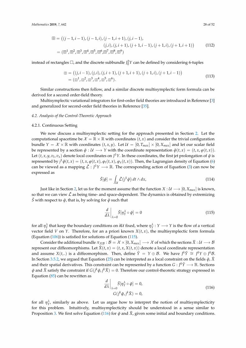
Mathematics 2019, 7, 642 28 of 52

=((j− 1, i− 1), (j− 1, i), (j− 1, i + 1), (j, i− 1),

(j, i), (j, i + 1), (j + 1, i− 1), (j + 1, i), (j + 1, i + 1))

= (1,2,3,4,5,6,7,8,9)

(112)

instead of rectangles , and the discrete subbundle J20Y can be defined by considering 6-tuples

=((j, i− 1), (j, i), (j, i + 1), (j + 1, i + 1), (j + 1, i), (j + 1, i− 1)

)= (1, 2, 3, 4, 5, 6).

(113)

Similar constructions then follow, and a similar discrete multisymplectic form formula can bederived for a second order-field theory.

Multisymplectic variational integrators for first-order field theories are introduced in Reference [3]and generalized for second-order field theories in Reference [35].

4.2. Analysis of the Control-Theoretic Approach

4.2.1. Continuous Setting

We now discuss a multisymplectic setting for the approach presented in Section 2. Let thecomputational spacetime be X = R×R with coordinates (t, x) and consider the trivial configurationbundle Y = X × R with coordinates (t, x, y). Let U = [0, Tmax] × [0, Xmax] and let our scalar fieldbe represented by a section ϕ : U −→ Y with the coordinate representation ϕ(t, x) = (t, x, ϕ(t, x)).Let (t, x, y, vt, vx) denote local coordinates on J1Y. In these coordinates, the first jet prolongation of ϕ isrepresented by j1 ϕ(t, x) = (t, x, ϕ(t, x), ϕt(t, x), ϕx(t, x)). Then, the Lagrangian density of Equation (6)can be viewed as a mapping L : J1Y −→ R. The corresponding action of Equation (3) can now beexpressed as

S[ϕ] =∫UL(

j1 ϕ)

dt ∧ dx, (114)

Just like in Section 2, let us for the moment assume that the function X : U −→ [0, Xmax] is known,so that we can view L as being time- and space-dependent. The dynamics is obtained by extremizingS with respect to ϕ, that is, by solving for ϕ such that

ddλ

∣∣∣∣λ=0

S[ηλY ϕ] = 0 (115)

for all ηλY that keep the boundary conditions on ∂U fixed, where ηλ

Y : Y −→ Y is the flow of a verticalvector field V on Y. Therefore, for an a priori known X(t, x), the multisymplectic form formula(Equation (106)) is satisfied for solutions of Equation (115).

Consider the additional bundle πXB : B = X × [0, Xmax] −→ X of which the sections X : U −→ Brepresent our diffeomorphisms. Let X(t, x) = (t, x, X(t, x)) denote a local coordinate representationand assume X(t, .) is a diffeomorphism. Then, define Y = Y ⊕ B. We have JkY ∼= JkY ⊕ JkB.In Section 3.5.2, we argued that Equation (25) can be interpreted as a local constraint on the fields ϕ, Xand their spatial derivatives. This constraint can be represented by a function G : JkY −→ R. Sectionsϕ and X satisfy the constraint if G(jk ϕ, jkX) = 0. Therefore our control-theoretic strategy expressed inEquation (85) can be rewritten as

ddλ

∣∣∣∣λ=0

S[ηλY ϕ] = 0,

G(jk ϕ, jkX) = 0,(116)

for all ηλY, similarly as above. Let us argue how to interpret the notion of multisymplecticity

for this problem. Intuitively, multisymplecticity should be understood in a sense similar toProposition 3. We first solve Equation (116) for ϕ and X, given some initial and boundary conditions.

Mathematics 2019, 7, 642 29 of 52

Then, we substitute this X into Equation (115). Let P be the set of solutions to this problem. Naturally,ϕ ∈ P . The multisymplectic form formula (Equation (106)) will be satisfied for all fields in P , but theconstraint G = 0 will be satisfied only for ϕ.

4.2.2. Discretization

Discretize the computational spacetime R×R by picking the discrete set of points tj = j · ∆t,xi = i · ∆x, and define X = (j, i) | j, i ∈ Z. Let X and X be the set of rectangles and 6-tuples inX , respectively. The discrete configuration bundle is Y = X ×R, and for convenience of notation, letthe elements of the fiber Yji be denoted by yj

i . Let U = (j, i) | j = 0, 1, . . . , M + 1, i = 0, 1, . . . , N + 1,where ∆x = Xmax/(N + 1) and ∆t = Tmax/(M + 1). Suppose we have a discrete Lagrangian L :J1Y −→ R and the corresponding discrete action S that approximates the action in Equation (114),where we assume that X(t, x) is known and of the form (10). A variational integrator is obtainedby solving

ddλ

∣∣∣∣λ=0

S[ϕλ] = 0 (117)

for a discrete section ϕ : U −→ Y, as described in Section 4.1. This integrator is multisymplectic, i.e.,the discrete multisymplectic form formula (Equation (110)) is satisfied.

Example: Midpoint rule.

In Equation (20), consider the 1-stage symplectic partitioned Runge–Kutta method with thecoefficients a11 = a11 = c1 = 1/2 and b1 = b1 = 1. This method is often called the midpoint rule andis a 2nd order member of the Gauss family of quadratures. It can be easily shown (see References [1,2])that the discrete Lagrangian of Equation (15) for this method is given by

Ld(tj, yj, tj+1, yj+1) = ∆t · LN

(yj + yj+1

2,

yj+1 − yj

∆t, tj +

12

∆t)

, (118)

where ∆t = tj+1 − tj and yj = (yj1, . . . , yj

N). Using Equations (5) and (13), we can write

Ld(tj, yj, tj+1, yj+1) =N

∑i=0

L(yj

i , yji+1, yj+1

i+1 , yj+1i), (119)

where we defined the discrete Lagrangian L : J1Y −→ R by the formula

L(yji , yj

i+1, yj+1i+1 , yj+1

i ) = ∆t∫ xi+1

xi

L(

ϕ(x), ϕx(x), ϕt(x), x, tj +12

∆t)

dx (120)

with

ϕ(x) =yj

i + yj+1i

2ηi(x) +

yji+1 + yj+1

i+12

ηi+1(x),

ϕx(x) =12

yji+1 − yj

i∆x

+12

yj+1i+1 − yj+1

i∆x

,

ϕt(x) =yj+1

i − yji

∆tηi(x) +

yj+1i+1 − yj

i+1∆t

ηi+1(x).

(121)

Given the Lagrangian density L as in Equation (6) and assuming X(t, x) is known, one canevaluate the integral in Equation (120) explicitly. It is now a straightforward calculation to showthat the discrete variational principle of Equation (117) for the discrete Lagrangian L as defined isequivalent to the discrete Euler–Lagrange Equation (103) for Ld and consequently to Equation (20).

This shows that the 2nd order Gauss method applied to Equation (20) defines a multisymplecticmethod in the sense of Equation (110). However, for other symplectic partitioned Runge–Kutta

Mathematics 2019, 7, 642 30 of 52

methods of interest to us, namely the 4th order Gauss and the 2nd/4th order Lobatto IIIA–IIIBmethods, it is not possible to isolate a discrete Lagrangian L that would only depend on four values yj

i ,

yji+1, yj+1

i+1 , and yj+1i . The mentioned methods have more internal stages, and Equation (20) couples

them in a nontrivial way. Effectively, at any given time step, the internal stages depend on all the valuesyj

1, . . . , yjN and yj+1

1 , . . . , yj+1N , and it is not possible to express the discrete Lagrangian of Equation (15)

as a sum similar to Equation (119). The resulting integrators are still variational, since they are derivedby applying the discrete variational principle of Equation (117) to some discrete action S, but thisaction cannot be expressed as the sum of L over all rectangles. Therefore, these integrators are notmultisymplectic, at least not in the sense of Equation (110).

Constraints.

Let the additional bundle be B = X × [0, Xmax], and denote by Xnj the elements of the fiber Bji.

Define Y = Y⊕B. We have JkY ∼= JkY⊕ JkB. Suppose G : JkY −→ R represents a discretization ofthe continuous constraint. For instance, one can enforce a uniform mesh by defining G : J1Y → R,G(j1 ϕ, j1X) = Xx − 1 at the continuous level. The discrete counterpart will be defined on the discretejet bundle J1Y by the following formula:

G(yji , yj

i+1, yj+1i+1 , yj+1

i , X ji , X j

i+1, X j+1i+1 , X j+1

i ) =X j

i+1 − X ji

∆x− 1. (122)

Arclength equidistribution can be realized by enforcing Equation (27), that is, G : J20 Y → R,

G(j20 ϕ, j20X) = α2 ϕx ϕxx + XxXxx. The discrete counterpart will be defined on the discrete sub-bundleJ20 Y by the following formula:

G(yl , Xr ) = α2(y3 − y2)2 + (X3 − X2)2 − α2(y2 − y1)2 − (X2 − X1)2, (123)

where, for convenience, we used the notation introduced in Equation (113) and l, r = 1, . . . , 6. Notethat Equation (123) coincides with Equation (28). In fact, gi in Equation (28) is nothing else but Gcomputed on an element of J2

0 Y over the base 6-tuple such that 2 = (j, i). The only difference isthat, in Equation (28), we assumed gi might depend on all the field values at a given time step, whileG only takes arguments locally, i.e., it depends on at most 6 field values on a given 6-tuple.

A numerical scheme is now obtained by simultaneously solving the discrete Euler–LagrangeEquation (109) resulting from Equation (117) and the equation G = 0. If we know yj−1

i , X j−1i , yj

i , and X ji

for i = 1, . . . , N, this system of equations allows us to solve for yj+1i , X j+1

i . This numerical scheme ismultisymplectic in the sense similar to Proposition 4. If we take X(t, x) to be a sufficiently smoothinterpolation of the values X j

i and substitute it in Equation (117), then the resulting multisymplectic

integrator will yield the same numerical values yj+1i .

4.3. Analysis of the Lagrange Multiplier Approach

4.3.1. Continuous Setting

We now turn to describing the Lagrange multiplier approach in a multisymplectic setting.Similarly as in Section 4.2, let the computational spacetime be X = R × [0, Xmax] withcoordinates (t, x) and consider the trivial configuration bundles πXY : Y = X × R −→ X andπXB : B = X × [0, Xmax] −→ X . Let our scalar field be represented by a section ϕ : X −→ Y withthe coordinate representation ϕ(t, x) = (t, x, ϕ(t, x)) and our diffeomorphism be represented by asection X : X −→ B with the local representation X(t, x) = (t, x, X(t, x)). Let the total configuration

Mathematics 2019, 7, 642 31 of 52

bundle be Y = Y ⊕ B. Then, the Lagrangian density of Equation (6) can be viewed as a mappingL : J1Y ∼= J1Y⊕ J1B −→ R. The corresponding action of Equation (3) can now be expressed as

S[ϕ, X] =∫UL(

j1 ϕ, j1X)

dt ∧ dx, (124)

where U = [0, Tmax]× [0, Xmax]. As before, the MMPDE constraint can be represented by a functionG : JkY −→ R. Two sections ϕ and X satisfy the constraint if

G(jk ϕ, jkX) = 0. (125)

Vakonomic formulation.

We now face the problem of finding the right equations of motion. We want to extremize theaction functional of Equation (124) in some sense, subject to the constraint in Equation (125). Note thatthe constraint is essentially nonholonomic, as it depends on the derivatives of the fields. AssumingG is a submersion, G = 0 defines a submanifold of JkY, but this submanifold will not in general bethe kth jet of any subbundle of Y. Two distinct approaches are possible here. One could follow theLagrange–d’Alembert principle and take variations of S first but choose variations V (vertical vectorfields on Y) such that the jet prolongations jkV are tangent to the submanifold G = 0 and then enforcethe constraint G = 0. On the other hand, one could consider the variational nonholonomic problem(also called vakonomic), and minimize S over the set of all sections (ϕ, X) that satisfy the constraintG = 0, that is, enforce the constraint before taking the variations. If the constraint is holonomic,both approaches yield the same equations of motion. However, if the constraint is nonholonomic,the resulting equations are in general different. Which equations are correct is really a matter ofexperimental verification. It has been established that the Lagrange–d’Alembert principle gives theright equations of motion for nonholonomic mechanical systems, whereas the vakonomic setting isappropriate for optimal control problems (see References [37–40]).

We will argue that the vakonomic approach is the right one in our case. In Proposition 5,we showed that in the unconstrained case extremizing S[φ] with respect to φ was equivalent toextremizing S[ϕ, X] with respect to ϕ, and in Proposition 6, we showed that extremizing with respectto X did not yield new information. This is because there was no restriction on the fields ϕ andX and, for any given X, there was a one-to-one correspondence between φ and ϕ given by theformula ϕ(t, x) = φ(t, X(t, x)), so extremizing over all possible ϕ was equivalent to extremizingover all possible φ. Now, let N be the set of all smooth sections (ϕ, X) that satisfy Equation (125)such that X(t, .) is a diffeomorphism for all t. It should be intuitively clear that, under appropriateassumptions on the mesh density function ρ, for any given smooth function φ(t, X), Equation (25)together with ϕ(t, x) = φ(t, X(t, x)) define a unique pair (ϕ, X) ∈ N (since our main purpose here isto only justify the application of the vakonomic approach, we do not attempt to specify those analyticassumptions precisely). Conversely, any given pair (ϕ, X) ∈ N defines a unique function φ throughthe formula φ(t, X) = ϕ(t, ξ(t, X)), where ξ(t, .) = X(t, .)−1, as in Section 3.1. Given this one-to-onecorrespondence and the fact that S[φ] = S[ϕ, X] by definition, we see that extremizing S with respectto all smooth φ is equivalent to extremizing S over all smooth sections (ϕ, X) ∈ N . We conclude thatthe vakonomic approach is appropriate in our case, since it follows from Hamilton’s principle for theoriginal, physically meaningful, action functional S.

Let us also note that our constraint depends on spatial derivatives only. Therefore, in the settingpresented in Sections 2 and 3 it can be considered holonomic, as it restricts the infinite-dimensionalconfiguration manifold of fields that we used as our configuration space. In that case, it is valid touse Hamilton’s principle and to minimize the action functional over the set of all allowable fields,i.e., those that satisfy the constraint G = 0. We did that by considering the augmented instantaneousLagrangian (86).

Mathematics 2019, 7, 642 32 of 52

In order to minimize S over the set of sections satisfying Equation (125), we will use thebundle-theoretic version of the Lagrange multiplier theorem, which we cite below after Reference [41].

Theorem 1 (Lagrange multiplier theorem). Let πM,E : E −→ M be an inner product bundle over asmooth manifold M, Ψ be a smooth section of πM,E , and h : M −→ R be a smooth function. SettingN = Ψ−1(0), the following are equivalent:

1. σ ∈ N is an extremum of h|N ,2. There exists an extremum σ ∈ E of h : E −→ R such that πM,E (σ) = σ,

where h(σ) = h(πM,E (σ))−⟨σ, Ψ(πM,E (σ))

⟩E .

Let us briefly review the ideas presented in Reference [41], adjusting the notation to our problemand generalizing when necessary. Let

C∞U (Y) = σ = (ϕ, X) : U ⊂ X −→ Y (126)

be the set of smooth sections of πX Y on U . Then, S : C∞U (Y) −→ R can be identified with h in

Theorem 1, whereM = C∞U (Y). Furthermore, define the trivial bundle

πXV : V = X ×R −→ X (127)

and let C∞U (V) be the set of smooth sections λ : U −→ V , which represent our Lagrange multipliers

and in local coordinates have the representation λ(t, x) = (t, x, λ(t, x)). The set C∞U (V) is an inner

product space with 〈λ1, λ2〉 =∫U λ1λ2 dt ∧ dx. Take

E = C∞U (Y)× C∞

U (V). (128)

This is an inner product bundle over C∞U (Y) with the inner product defined by⟨

(σ, λ1), (σ, λ2)⟩E= 〈λ1, λ2〉. (129)

We now have to construct a smooth section Ψ : C∞U (Y) −→ E that will realize our constraint of

Equation (125). Define the fiber-preserving mapping G : JkY −→ V such that for ϑ ∈ JkY

G(ϑ) =(πX ,JkY(ϑ), G(ϑ)

). (130)

For instance, for k = 1, in local coordinates, we have G(t, x, y, vt, vx) = (t, x, G(t, x, y, vt, vx)).Then, we can define

Ψ(σ) = (σ, G jkσ). (131)

The set of allowable sections N ⊂ C∞U (Y) is now defined by N = Ψ−1(0). That is, (ϕ, X) ∈ N

provided that G(jk ϕ, jkX) = 0.The augmented action functional SC : E −→ R is now given by

SC[σ] = S[πM,E (σ)]−⟨σ, Ψ(πM,E (σ))

⟩E , (132)

or denoting σ = (ϕ, X, λ)

SC[ϕ, X, λ] = S[ϕ, X]−⟨λ, G (jk ϕ, jkX)

⟩=∫UL(

j1 ϕ, j1X)

dt ∧ dx−∫U

λ(t, x) G(jk ϕ, jkX) dt ∧ dx

=∫U

[L(

j1 ϕ, j1X)− λ(t, x) G(jk ϕ, jkX)

]dt ∧ dx.

(133)

Mathematics 2019, 7, 642 33 of 52

Theorem 1 states that, if (ϕ, X, λ) is an extremum of SC, then (ϕ, X) extremizes S over the setN of sections satisfying the constraint G = 0. Note that using the multisymplectic formalism weobtained the same result as Equation (86) in the instantaneous formulation, where we could treat G asa holonomic constraint. The dynamics is obtained by solving for a triple (ϕ, X, λ) such that

ddε

∣∣∣∣ε=0

SC[ηεY ϕ, ηε

B X, ηεV λ] = 0 (134)

for all ηεY, ηε

B , ηεV that keep the boundary conditions on ∂U fixed, where ηε denotes the flow of vertical

vector fields on respective bundles.Note that we can define YC = Y ⊕ B ⊕ V and LC : JkYC −→ R by setting LC = L − λ · G,

i.e., we can consider a kth-order field theory. If k = 1, 2 then an appropriate multisymplectic formformula in terms of the fields ϕ, X, and λ will hold. Presumably, this can be generalized for k > 2 usingthe techniques put forth in Reference [35]. However, it is an interesting question whether there existsany multisymplectic form formula defined in terms of ϕ, X, and objects on JkY only. It appears to bean open problem. This would be the multisymplectic analog of the fact that the flow of a constrainedmechanical system is symplectic on the constraint submanifold of the configuration space.

4.3.2. Discretization

Let us use the same discretization as discussed in Section 4.2. Assume we have a discreteLagrangian L : J1Y −→ R, the corresponding discrete action S[ϕ, X], and a discrete constraintG : J1Y −→ R or G : J2

0 Y −→ R. Note that S is essentially a function of 2MN variables and thatwe want to extremize it subject to the set of algebraic constraints G = 0. The standard Lagrangemultiplier theorem proved in basic calculus textbooks applies here. However, let us work out a discretecounterpart of the formalism introduced at the continuous level. This will facilitate the discussion ofthe discrete notion of multisymplecticity. Let

CU (Y) = σ = (ϕ, X) : U ⊂ X −→ Y (135)

be the set of discrete sections of πX Y : Y −→ X . Similarly, define the discrete bundle V = X ×R,and let CU0(V) be the set of discrete sections λ : U0 −→ V representing the Lagrange multipliers,

where U0 ⊂ U is defined below. Let λ(j, i) = (j, i, λ(j, i)) with λji ≡ λ(j, i) be the local representation.

The set CU0(V) is an inner product space with 〈λ, µ〉 = ∑(j,i)∈U0λ

jiµ

ji . Take E = CU (Y) × CU0(V).

Just like at the continuous level, E is an inner product bundle. However, at the discrete level, it is moreconvenient to define the inner product on E in a slightly modified way. Since there are some nuancesin the notation, let us consider the cases k = 1 and k = 2 separately.

Case k = 1.

Let U0 = (j, i) ∈ U | j ≤ M, i ≤ N. Define the trivial bundle V = X ×R and let CU(V) bethe set of all sections of V defined on U. For a given section λ ∈ CU0(V), we define its extensionλ ∈ CU(V) by

λ() =(, λ(1)

), (136)

that is, λ assigns to the square the value that λ takes on the first vertex of that square. Note that thisoperation is invertible: Given a section of CU(V), we can uniquely determine a section of CU0(V).We can define the inner product

〈λ, µ〉 = ∑⊂U

λ(1)µ(1). (137)

One can easily see that we have 〈λ, µ〉 = 〈λ, µ〉, so by a slight abuse of notation, we can use thesame symbol 〈., .〉 for both inner products. It will be clear from the context which definition should beinvoked. We can now define an inner product on the fibers of E as

Mathematics 2019, 7, 642 34 of 52

⟨(σ, λ), (σ, µ)

⟩E= 〈λ, µ〉 = 〈λ, µ〉. (138)

Let us now construct a section Ψ : CU (Y) −→ E that will realize our discrete constraint G. First,in analogy to Equation (130), define the fiber-preserving mapping G : J1Y −→ V such that

G(yl , Xr ) =(, G(yl , Xr )

), (139)

where l, r = 1, 2, 3, 4. We now define Ψ by requiring that for σ ∈ CU (Y) the extension of Ψ(σ), definedsimilar to Equation (136), is given by

Ψ(σ) = (σ, G j1σ). (140)

The set of allowable sections N ⊂ CU (Y) is now defined by N = Ψ−1(0)—that is, (ϕ, X) ∈ N ,provided that G(j1 ϕ, j1X) = 0 for all ∈ U. The augmented discrete action SC : E −→ R is therefore

SC[σ, λ] = S[σ]−⟨(σ, λ), Ψ(σ)

⟩E

= S[σ]−⟨

λ, G j1σ⟩

= ∑⊂U

L(j1σ)− ∑⊂U

λ(1)G(j1σ)

= ∑⊂U

(L(j1σ)− λ(1)G(j1σ)

).

(141)

By the standard Lagrange multiplier theorem, if (ϕ, X, λ) is an extremum of SC, then (ϕ, X) isan extremum of S over the set N of sections satisfying the constraint G = 0. The discrete Hamiltonprinciple can be expressed as

ddε

∣∣∣∣ε=0

SC[ϕε, Xε, λε] = 0 (142)

for all vector fields V on Y, W on B, and Z on V that keep the boundary conditions on ∂U fixed,

where ϕε(j, i) = FVjiε (ϕ(j, i)) and F

Vjiε is the flow of Vji on R, and similarly for Xε and λε. The discrete

Euler–Lagrange equations can be conveniently computed if in Equation (142) one focuses on some(j, i) ∈ intU . With the convention ϕ(j, i) = yj

i , X(j, i) = X ji , and λ(j, i) = λ

ji , we write the terms of SC

containing yji , X j

i and λji explicitly as

SC = . . . + L(yj

i , yji+1, yj+1

i+1 , yj+1i , X j

i , X ji+1, X j+1

i+1 , X j+1i)

+ L(yj

i−1, yji , yj+1

i , yj+1i−1 , X j

i−1, X ji , X j+1

i , X j+1i−1

)+ L

(yj−1

i−1 , yj−1i , yj

i , yji−1, X j−1

i−1 , X j−1i , X j

i , X ji−1

)+ L

(yj−1

i , yj−1i+1 , yj

i+1, yji , X j−1

i , X j−1i+1 , X j

i+1, X ji)

+ λji G(yj

i , yji+1, yj+1

i+1 , yj+1i , X j

i , X ji+1, X j+1

i+1 , X j+1i)

+ λji−1G

(yj

i−1, yji , yj+1

i , yj+1i−1 , X j

i−1, X ji , X j+1

i , X j+1i−1

)+ λ

j−1i−1G

(yj−1

i−1 , yj−1i , yj

i , yji−1, X j−1

i−1 , X j−1i , X j

i , X ji−1

)+ λ

j−1i G

(yj−1

i , yj−1i+1 , yj

i+1, yji , X j−1

i , X j−1i+1 , X j

i+1, X ji)+ . . .

(143)

The discrete Euler–Lagrange equations are obtained by differentiating with respect to yji , X j

i ,

and λji and can be written compactly as

Mathematics 2019, 7, 642 35 of 52

∑l,

(j,i)=l

[∂L∂yl (y1 , . . . , y4 ,X1 , . . . , X4)+

λ1∂G∂yl (y1 , . . . , y4 , X1 , . . . , X4)

]= 0,

∑l,

(j,i)=l

[∂L∂Xl (y1 , . . . , y4 ,X1 , . . . , X4)+

λ1∂G∂Xl (y1 , . . . , y4 , X1 , . . . , X4)

]= 0,

G(yj

i , yji+1, yj+1

i+1 , yj+1i , X j

i , X ji+1, X j+1

i+1 , X j+1i)= 0

(144)

for all (j, i) ∈ intU . If we know yj−1i , X j−1

i , yji , X j

i , and λj−1i for i = 1, . . . , N, this system of equations

allows us to solve for yj+1i , X j+1

i , and λji .

Note that we can define YC = Y ⊕ B ⊕ V and the augmented Lagrangian LC : J1YC −→ Rby setting

LC(j1 ϕ, j1X, j1λ) = L(j1 ϕ, j1X)− λ(1) · G(j1 ϕ, j1X), (145)

we can consider an unconstrained field theory in terms of the fields ϕ, X, and λ. Then, the solutions ofEquation (144) satisfy the multisymplectic form formula (Equation (110)) in terms of objects definedon J1YC.

Case k = 2.

Let U0 = (j, i) ∈ U | j ≤ M, 1 ≤ i ≤ N. Define the trivial bundle V = X ×R, and let CU(V)be the set of all sections of V defined on U. For a given section λ ∈ CU0(V), we define its extensionλ ∈ CU(V) by

λ() =(, λ(2)

), (146)

that is, λ assigns to the 6-tuple the value that λ takes on the second vertex of that 6-tuple. Like before,this operation is invertible. We can define the inner product

〈λ, µ〉 = ∑⊂U

λ(2)µ(2) (147)

and the inner product on E as in Equation (138). Define the fiber-preserving mapping G : J20 Y −→ V

such thatG(yl , Xr ) =

(, G(yl , Xr )

), (148)

where l, r = 1, . . . , 6. We now define Ψ by requiring that, for σ ∈ CU (Y), the extension of Ψ(σ), definedsimilar to Equation (146), is given by

Ψ(σ) = (σ, G j20σ). (149)

Again, the set of allowable sections is N = Ψ−1(0). That is, (ϕ, X) ∈ N , provided thatG(j20 ϕ, j20X) = 0 for all ∈ U. The augmented discrete action SC : E −→ R is therefore

Mathematics 2019, 7, 642 36 of 52

SC[σ, λ] = S[σ]−⟨(σ, λ), Ψ(σ)

⟩E

= S[σ]−⟨

λ, G j20σ⟩

= ∑⊂U

L(j1σ)− ∑⊂U

λ(2)G(j20σ).

(150)

Writing out the terms involving yji , X j

i , and λji explicitly, as in Equation (143), and invoking the

discrete Hamilton principle (142), one obtains the discrete Euler–Lagrange equations, which can becompactly expressed as

∑l,

(j,i)=l

∂L∂yl (y1 , . . . , y4 ,X1 , . . . , X4)+

∑l,

(j,i)=l

λ2∂G∂yl (y1 , . . . , y6 , X1 , . . . , X6) = 0,

∑l,

(j,i)=l

∂L∂Xl (y1 , . . . , y4 ,X1 , . . . , X4)+

∑l,

(j,i)=l

λ2∂G∂Xl (y1 , . . . , y6 , X1 , . . . , X6) = 0,

G(yj

i−1, yji , yj

i+1, yj+1i+1 , yj+1

i , yj+1i−1 , X j

i−1, X ji , X j

i+1, X j+1i+1 , X j+1

i , X j+1i−1

)= 0

(151)

for all (j, i) ∈ intU . If we know yj−1i , X j−1

i , yji , X j

i , and λj−1i for i = 1, . . . , N, this system of equations

allows us to solve for yj+1i , X j+1

i and λji .

Let us define the extension Lext : J20 Y −→ R of the Lagrangian density L by setting

Lext(y1 , . . . , X6) =

L(y1 , . . . , X4) if 2 = (j, 0), (j, N + 1),

where = ∩ U ,12 ∑⊂ L(y1 , . . . , X4) otherwise.

(152)

Let us also set G(y1 , . . . , X4) = 0 if 2 = (j, 0), (j, N + 1). Define A = |2, 5 ∈ U. Then,Equation (150) can be written as

SC[σ, λ] = ∑∈A

[Lext(j20σ)− λ(2)G(j20σ)

]= ∑

∈ALC(j20σ, j20λ), (153)

where the last equality defines the augmented Lagrangian LC : J20 YC −→ R for YC = Y ⊕ B ⊕ V .

Therefore, we can consider an unconstrained second-order field theory in terms of the fields ϕ, X,and λ, and the solutions of Equation (151) will satisfy a discrete multisymplectic form formula verysimilar to the one proved in Reference [35]. The only difference is the fact that the authors analyzed adiscretization of the Camassa–Holm equation and were able to consider an even smaller sub-bundleof the second jet of the configuration bundle. As a result, it was sufficient for them to consider adiscretization based on squares rather than 6-tuples . In our case, there will be six discrete 2-formsΩl

LCfor l = 1, . . . , 6 instead of just four.

Mathematics 2019, 7, 642 37 of 52

Remark 5. In both cases, we showed that our discretization leads to integrators that are multisymplectic on theaugmented jets JkYC. However, just like in the continuous setting, it is an interesting problem whether thereexists a discrete multisymplectic form formula in terms of objects defined on JkY only.

Example: Trapezoidal rule.

Consider the semi-discrete Lagrangian in Equation (44). We can use the trapezoidal rule to definethe discrete Lagrangian in Equation (14) as

Ld(yj, X j, yj+1, X j+1) =∆t2

LN

(yj, X j,

yj+1 − yj

∆t,

X j+1 − X j

∆t

)+

∆t2

LN

(yj+1, X j+1,

yj+1 − yj

∆t,

X j+1 − X j

∆t

),

(154)

where yj = (yj1, . . . , yj

N) and X j = (X j1, . . . , X j

N). The constrained version (see Reference [2]) of theDiscrete Euler–Lagrange Equation (103) takes the form

D2 Ld(qj−1, qj) + D1 Ld(qj, qj+1) = Dg(qj)Tλj,

g(qj+1) = 0,(155)

where for brevity qj = (yj1, X j

1, . . . , yjN , X j

N), λj = (λj1, . . . , λ

jN) and g is an adaptation constraint,

for instance Equation (28). If qj−1, qj are known, then Equation (155) can be used to compute qj+1

and λj. It is easy to verify that the condition of Equation (94) is enough to ensure solvability ofEquation (155), assuming the time step ∆t is sufficiently small, so there is no need to introduceslack degrees of freedom as in Equation (95). If the mass matrix of Equation (47) was constant andnon-singular, then Equation (155) would result in the SHAKE algorithm, or in the RATTLE algorithmif one passes to the position-momentum formulation (see References [1,2]).

Using Equations (38) and (41), we can write

Ld(yj, X j, yj+1, X j+1) =N

∑i=0

L(yj

i , yji+1, yj+1

i+1 , yj+1i , X j

i , X ji+1, X j+1

i+1 , X j+1i), (156)

where we defined the discrete Lagrangian L : J1Y −→ R by the formula

L(

yji , yj

i+1, yj+1i+1 , yj+1

i , X ji , X j

i+1, X j+1i+1 , X j+1

i

)=

∆t2

∫ xi+1

xi

L(

ϕj(x), X j(x), ϕjx(x), X j

x(x), ϕt(x), Xt(x))

dx

+∆t2

∫ xi+1

xi

L(

ϕj+1(x), X j+1(x), ϕj+1x (x), X j+1

x (x), ϕt(x), Xt(x))

dx

(157)

withϕj(x) = yj

iηi(x) + yji+1ηi+1(x),

ϕjx(x) =

yji+1 − yj

i∆x

,

ϕt(x) =yj+1

i − yji

∆tηi(x) +

yj+1i+1 − yj

i+1∆t

ηi+1(x),

(158)

and similarly for X(x). Given the Lagrangian density L as in Equation (43), one can compute theintegrals in Equation (157) explicitly. Suppose that the adaptation constraint g has a “local” structure,for instance

gi(yj, X j) = G(yji , yj

i+1, yj+1i+1 , yj+1

i , X ji , X j

i+1, X j+1i+1 , X j+1

i ), (159)

Mathematics 2019, 7, 642 38 of 52

as in Equation (122) or

gi(yj, X j) = G(yl , Xr ), where 2 = (j, i), (160)

as in Equation (123). It is straightforward to show that Equation (144) or Equation (151) are equivalentto Equation (155), that is, the variational integrator defined by Equation (155) is also multisymplectic.

For reasons similar to the ones pointed out in Section 4.2, the 2nd and 4th order Lobatto IIIA–IIIBmethods that we used for our numerical computations are not multisymplectic.

5. Numerical Results

5.1. The Sine–Gordon Equation

We applied the methods discussed in the previous sections to the Sine–Gordon equation

∂2φ

∂t2 −∂2φ

∂X2 + sin φ = 0. (161)

This equation results from the (1+1)-dimensional scalar field theory with the Lagrangian density

L(φ, φX , φt) =12

φ2t −

12

φ2X − (1− cos φ). (162)

The Sine–Gordon equation arises in many physical applications. For instance, it governs thepropagation of dislocations in crystals, the evolution of magnetic flux in a long Josephson-junctiontransmission line, or the modulation of a weakly unstable baroclinic wave packet in a two-layer fluid.It also has applications in the description of one-dimensional organic conductors, one-dimensionalferromagnets, and liquid crystals or in particle physics as a model for baryons (see References [42,43]).

The Sine–Gordon equation has interesting soliton solutions. A single soliton traveling at the speedv is given by

φS(X, t) = 4 arctan[

exp(

X− X0 − vt√1− v2

)]. (163)

It is depicted in Figure 2. The backscattering of two solitons, each traveling with the velocity v,is described by the formula

φSS(X, t) = 4 arctan

[v sinh( X√

1−v2 )

cosh( vt√1−v2 )

]. (164)

0

X

φ π

2π

X0+vt

Figure 2. The single soliton solution of the Sine–Gordon equation.

Mathematics 2019, 7, 642 39 of 52

It is depicted in Figure 3. Note that if we restrict X ≥ 0, then this formula also gives a single solitonsolution satisfying the boundary condition φ(0, t) = 0, that is, a soliton bouncing from a rigid wall.

0

φ

0

φ

0

X

φ

t<0

t=0

t>0

−2π

−π

0

π

2π

−2π

−π

0

π

2π

−2π

−π

π

2π

0

Figure 3. The two-soliton solution of the Sine–Gordon equation.

5.2. Generating Consistent Initial Conditions

Suppose we specify the following initial conditions

φ(X, 0) = a(X),

φt(X, 0) = b(X),(165)

and assume they are consistent with the boundary conditions stated in Equation (2). In order todetermine appropriate consistent initial conditions for Equations (18) and (98), we need to solveseveral equations. First, we solve for the yi’s and Xi’s. We have y0 = φL, yN+1 = φR, X0 = 0,and XN+1 = Xmax. The rest are determined by solving the system

yi = a(Xi),

0 = gi(y1, . . . , yN , X1, . . . , XN),(166)

for i = 1, . . . , N. This is a system of 2N nonlinear equations for 2N unknowns. We solve it usingNewton’s method. Note, however, that we do not a priori know good starting points for Newton’s

Mathematics 2019, 7, 642 40 of 52

iterations. If our initial guesses are not close enough to the desired solution, the iterations may convergeto the wrong solution or may not converge at all. In our computations, we used the constraints givenin Equation (28). We found that a very simple variant of a homotopy continuation method workedvery well in our case. Note that for α = 0 Equation (28) generates a uniform mesh. In order tosolve Equation (166) for some α > 0, we split [0, α] into d subintervals by picking αk = (k/d) · αfor k = 1, . . . , d. We then solved Equation (166) with α1 using the uniformly spaced mesh pointsX(0)

i = (i/(N + 1)) ·Xmax as our initial guess, resulting in X(1)i and y(1)i . Then, we solved Equation (166)

with α2 using X(1)i and y(1)i as the initial guesses, resulting in X(2)

i and y(2)i . Continuing in this fashion,

we got X(d)i and y(d)i as the numerical solution to Equation (166) for the original value of α. Note that

for more complicated initial conditions and constraint functions, predictor–corrector methods shouldbe used—see Reference [44] for more information. Another approach to solving Equation (166) couldbe based on relaxation methods (see References [7,8]).

Next, we solve for the initial values of the velocities yi and Xi. Since ϕ(x, t) = φ(X(x, t), t),we have ϕt(x, t) = φX(X(x, t), t)Xt(x, t) + φt(X(x, t), t). We also require that the velocities beconsistent with the constraints. Hence, the linear system is

yi = a′(Xi)Xi + b(Xi), i = 1, . . . , N

0 =∂g∂y

(y, X)y +∂g∂X

(y, X)X.(167)

This is a system of 2N linear equations for the 2N unknowns yi and Xi, where y = (y1, . . . , yN) andX = (X1, . . . , XN). We can use those velocities to compute the initial values of the conjugate momenta.For the control-theoretic approach, we use pi = ∂LN/∂yi, as in Section 2.3, and for the Lagrangemultiplier approach, we use Equation (46). In addition, for the Lagrange multiplier approach, we alsohave the initial values for the slack variables ri = 0 and their conjugate momenta Bi = ∂LA

N/∂ri = 0.It is also useful to use Equation (93) to compute the initial values of the Lagrange multipliers λi thatcan be used as initial guesses in the first iteration of the Lobatto IIIA–IIIB algorithm. The initial guessesfor the slack Lagrange multipliers are trivially µi = 0. Note that both λ and µ are algebraic variables,so their values at each time step are completely determined by the Lobatto IIIA–IIIB algorithm (seeReferences [1,27,28] for details), and therefore no further initial or boundary conditions are necessary.

5.3. Convergence

In order to test the convergence of our methods as the number of mesh points N is increased,we considered a single soliton bouncing from two rigid walls at X = 0 and X = Xmax = 25.We imposed the boundary conditions φL = 0 and φR = 2π, and as initial conditions we usedEquation (163) with X0 = 12.5 and v = 0.9. It is possible to obtain the exact solution to this problem byconsidering a multi-soliton solution to Equation (161) on the whole real line. Such a solution can beobtained using a Bäcklund transformation (see References [42,43]). However, the formulas quicklybecome complicated and, technically, one would have to consider an infinite number of solitons.Instead, we constructed a nearly exact solution by approximating the boundary interactions with (164):

φexact(X, t) =

φSS(X− Xmax, t− (4n + 1)T

)+ 2π if t ∈

[4nT, (4n + 2)T

),

φSS(X, t− (4n + 3)T

)if t ∈

[(4n + 2)T, (4n + 4)T

),

(168)

where n is an integer number and T satisfies φSS(Xmax/2, T) = π (we numerically found T ≈ 13.84).Given how fast the functions given in Equations (163) and (164) approach their asymptotic values, onemay check that Equation (168) can be considered exact to machine precision.

We performed numerical integration with the constant time step ∆t = 0.01 up to the timeTmax = 50. For the control-theoretic strategy, we used the 1-stage and 2-stage Gauss method (2nd and4th order, respectively), and the 2-stage and 3-stage Lobatto IIIA–IIIB method (also 2nd/4th order).

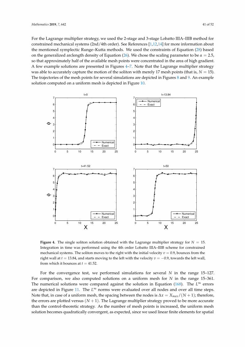
Mathematics 2019, 7, 642 41 of 52

For the Lagrange multiplier strategy, we used the 2-stage and 3-stage Lobatto IIIA–IIIB method forconstrained mechanical systems (2nd/4th order). See References [1,12,14] for more information aboutthe mentioned symplectic Runge–Kutta methods. We used the constraints of Equation (28) basedon the generalized arclength density of Equation (26). We chose the scaling parameter to be α = 2.5,so that approximately half of the available mesh points were concentrated in the area of high gradient.A few example solutions are presented in Figures 4–7. Note that the Lagrange multiplier strategywas able to accurately capture the motion of the soliton with merely 17 mesh points (that is, N = 15).The trajectories of the mesh points for several simulations are depicted in Figures 8 and 9. An examplesolution computed on a uniform mesh is depicted in Figure 10.

0 5 10 15 20 25

0

1

2

3

4

5

6

7

φ

t=0

Numerical

Exact

0 5 10 15 20 25

0

1

2

3

4

5

6

7

t=13.84

0 5 10 15 20 25

0

1

2

3

4

5

6

7

t=41.52

X

φ

0 5 10 15 20 25

0

1

2

3

4

5

6

7

t=50

X

Numerical

Exact

Numerical

Exact

Numerical

Exact

Figure 4. The single soliton solution obtained with the Lagrange multiplier strategy for N = 15.Integration in time was performed using the 4th order Lobatto IIIA–IIIB scheme for constrainedmechanical systems. The soliton moves to the right with the initial velocity v = 0.9, bounces from theright wall at t = 13.84, and starts moving to the left with the velocity v = −0.9, towards the left wall,from which it bounces at t = 41.52.

For the convergence test, we performed simulations for several N in the range 15–127.For comparison, we also computed solutions on a uniform mesh for N in the range 15–361.The numerical solutions were compared against the solution in Equation (168). The L∞ errorsare depicted in Figure 11. The L∞ norms were evaluated over all nodes and over all time steps.Note that, in case of a uniform mesh, the spacing between the nodes is ∆x = Xmax/(N + 1); therefore,the errors are plotted versus (N + 1). The Lagrange multiplier strategy proved to be more accuratethan the control-theoretic strategy. As the number of mesh points is increased, the uniform meshsolution becomes quadratically convergent, as expected, since we used linear finite elements for spatial

Mathematics 2019, 7, 642 42 of 52

discretization. The control-theoretic strategy also shows near quadratic convergence, whereas theLagrange multiplier method seems to converge slightly slower. While there are very few analyticalresults regarding the convergence of r-adaptive methods, it has been observed that the rate ofconvergence depends on several factors, including the chosen mesh density function. Our results areconsistent with the convergence rates reported in References [45,46]. Both papers deal with the viscousBurgers’ equation but consider different initial conditions. Computations with the arc-length densityfunction converged only linearly in Reference [45] but quadratically in Reference [46].

0 5 10 15 20 25

0

1

2

3

4

5

6

7

φ

t=0

Numerical

Exact

0 5 10 15 20 25

0

1

2

3

4

5

6

7

t=13.84

0 5 10 15 20 25

0

1

2

3

4

5

6

7

t=41.52

X

φ

0 5 10 15 20 25

0

1

2

3

4

5

6

7

t=50

X

Numerical

Exact

Numerical

Exact

Numerical

Exact

Figure 5. The single soliton solution obtained with the Lagrange multiplier strategy for N = 31:Integration in time was performed using the 4th-order Lobatto IIIA–IIIB scheme for constrainedmechanical systems.

Version July 3, 2019 submitted to Mathematics 45 of 56

0 5 10 15 20 25

0

1

2

3

4

5

6

7

φ

t=0

NumericalExact

0 5 10 15 20 25

0

1

2

3

4

5

6

7t=13.84

0 5 10 15 20 25

0

1

2

3

4

5

6

7t=41.52

X

φ

0 5 10 15 20 25

0

1

2

3

4

5

6

7t=50

X

NumericalExact

NumericalExact

NumericalExact

Figure 6. The single soliton solution obtained with the control-theoretic strategy for N = 22. Integrationin time was performed using the 4-th order Gauss scheme. Integration with the 4-th order LobattoIIIA-IIIB yields a very similar level of accuracy.

Figure 6. Cont.

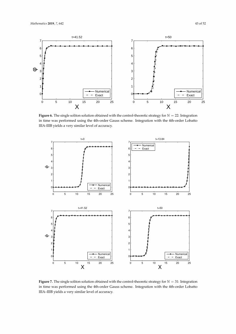
Mathematics 2019, 7, 642 43 of 52

Version July 3, 2019 submitted to Mathematics 45 of 56

0 5 10 15 20 25

0

1

2

3

4

5

6

7

φ

t=0

NumericalExact

0 5 10 15 20 25

0

1

2

3

4

5

6

7t=13.84

0 5 10 15 20 25

0

1

2

3

4

5

6

7t=41.52

X

φ

0 5 10 15 20 25

0

1

2

3

4

5

6

7t=50

X

NumericalExact

NumericalExact

NumericalExact

Figure 6. The single soliton solution obtained with the control-theoretic strategy for N = 22. Integrationin time was performed using the 4-th order Gauss scheme. Integration with the 4-th order LobattoIIIA-IIIB yields a very similar level of accuracy.

Figure 6. The single soliton solution obtained with the control-theoretic strategy for N = 22: Integrationin time was performed using the 4th-order Gauss scheme. Integration with the 4th-order LobattoIIIA-IIIB yields a very similar level of accuracy.

0 5 10 15 20 25

0

1

2

3

4

5

6

7

φ

t=0

Numerical

Exact

0 5 10 15 20 25

0

1

2

3

4

5

6

7

t=13.84

0 5 10 15 20 25

0

1

2

3

4

5

6

7

t=41.52

X

φ

0 5 10 15 20 25

0

1

2

3

4

5

6

7

t=50

X

Numerical

Exact

Numerical

Exact

Numerical

Exact

Figure 7. The single soliton solution obtained with the control-theoretic strategy for N = 31: Integrationin time was performed using the 4th-order Gauss scheme. Integration with the 4th-order LobattoIIIA–IIIB yields a very similar level of accuracy.

Mathematics 2019, 7, 642 44 of 52

0 5 10 15 20 250

5

10

15

20

25

30

35

40

45

50

X

t

0 5 10 15 20 250

5

10

15

20

25

30

35

40

45

50

X

t

Figure 8. The mesh point trajectories (with zoomed-in insets) for the Lagrange multiplier strategyfor N = 22 (left) and N = 31 (right): Integration in time was performed using the 4th-order LobattoIIIA–IIIB scheme for constrained mechanical systems.

0 5 10 15 20 250

5

10

15

20

25

30

35

40

45

50

X

t

0 5 10 15 20 250

5

10

15

20

25

30

35

40

45

50

X

t

Figure 9. The mesh point trajectories (with zoomed-in insets) for the control-theoretic strategy forN = 22 (left) and N = 31 (right): Integration in time was performed using the 4th-order Gauss scheme.Integration with the 4th-order Lobatto IIIA–IIIB yields a very similar result.

5.4. Energy Conservation

As we pointed out in Section 2.6, the true power of variational and symplectic integratorsfor mechanical systems lies in their excellent conservation of energy and other integrals of motion,even when a big time step is used. In order to test the energy behavior of our methods, we performedsimulations of the Sine–Gordon equation over longer time intervals. We considered two solitonsbouncing from each other and from two rigid walls at X = 0 and Xmax = 25. We imposed the boundaryconditions φL = −2π and φR = 2π, and as initial conditions we used φ(X, 0) = φSS(X − 12.5,−5)with v = 0.9. We ran our computations on a mesh consisting of 27 nodes (N = 25). Integration wasperformed with the time step ∆t = 0.05, which is rather large for this type of simulations. The scalingparameter in Equation (28) was set to α = 1.5, so that approximately half of the available mesh pointswere concentrated in the areas of high gradient. An example solution is presented in Figure 12.

Mathematics 2019, 7, 642 45 of 52

0 5 10 15 20 25

0

1

2

3

4

5

6

7

φ

t=0

Numerical

Exact

0 5 10 15 20 25

0

1

2

3

4

5

6

7

t=13.84

0 5 10 15 20 25

0

1

2

3

4

5

6

7

t=41.52

X

φ

0 5 10 15 20 25

0

1

2

3

4

5

6

7

t=50

X

Numerical

Exact

Numerical

Exact

Numerical

Exact

Figure 10. The single soliton solution computed on a uniform mesh with N = 31: Integration in timewas performed using the 4th-order Gauss scheme. Integration with the 4th-order Lobatto IIIA–IIIByields a very similar level of accuracy.

16 23 32 45 64 91 128 181 256 362

10−2

10−1

100

101

N+1

L∞

err

or

Lagrange multiplier

Control−theoretic

Uniform

~(N+1)−1.88

~(N+1)−1.88

~(N+1)−1.62

Figure 11. Comparison of the convergence rates of the discussed methods: Integration in time wasperformed using the 4th-order Lobatto IIIA–IIIB method for constrained systems in case of the Lagrangemultiplier strategy and the 4th-order Gauss scheme in case of both the control-theoretic strategy and theuniform mesh simulation. The 4th-order Lobatto IIIA–IIIB scheme for the control-theoretic strategy andthe uniform mesh simulation yield a very similar level of accuracy. Also, using 2nd-order integratorsgives very similar error plots.

Mathematics 2019, 7, 642 46 of 52

0 5 10 15 20 25

−6

−4

−2

0

2

4

6φ

t=0

Lagrange multiplier

Control−theoretic

Exact

0 5 10 15 20 25

−6

−4

−2

0

2

4

6

t=170.45

0 5 10 15 20 25

−6

−4

−2

0

2

4

6

t=322.1

X

φ

0 5 10 15 20 25

−6

−4

−2

0

2

4

6

t=494.45

X

Lagrange multiplier

Control−theoretic

Exact

Lagrange multiplier

Control−theoretic

Exact

Lagrange multiplier

Control−theoretic

Exact

Figure 12. The two-soliton solution obtained with the control-theoretic and Lagrange multiplierstrategies for N = 25. Integration in time was performed using the 4th-order Gauss quadraturefor the control-theoretic approach and the 4th-order Lobatto IIIA–IIIB quadrature for constrainedmechanical systems in case of the Lagrange multiplier approach. The solitons initially move towardseach other with the velocities v = 0.9, then bounce off of each other at t = 5 and start movingtowards the walls, from which they bounce at t = 18.79. The solitons bounce off of each other again att = 32.57. This solution is periodic in time with the period Tperiod = 27.57. The nearly exact solutionwas constructed in a similar fashion as Equation (168). As the simulation progresses, the Lagrangemultiplier solution gets ahead of the exact solution, whereas the control-theoretic solution lags behind.

The exact energy of the two-soliton solution can be computed using Equation (7). It is possible tocompute that integral explicitly to obtain E = 16/

√1− v2 ≈ 36.71. The energy associated with the

semi-discrete Lagrangian in Equation (44) can be expressed by the formula

EN =12

qT MN(q) q + RN(q), (169)

where RN was defined in Equation (88) and for our Sine–Gordon system is given by

RN(q) =N

∑k=0

[12

(yk+1 − ykXk+1 − Xk

)2

+ 1− sin yk+1 − sin ykyk+1 − yk

](Xk+1 − Xk), (170)

and MN is the mass matrix in Equation (47). The energy EN is an approximation to Equation (7) if theintegrand is sampled at the nodes X0, . . ., XN+1 and then piecewise linearly approximated. Therefore,we used EN to compute the energy of our numerical solutions.

Mathematics 2019, 7, 642 47 of 52

The energy plots for the Lagrange multiplier strategy are depicted in Figure 13. We can see thatthe energy stays nearly constant in the presented time interval, showing only mild oscillations, whichare reduced as a higher order of integration in time is used. The energy plots for the control-theoreticstrategy are depicted in Figure 14. In this case, the discrete energy is more erratic and not as nearlypreserved. Moreover, the symplectic Gauss and Lobatto methods show virtually the same energybehavior as the non-symplectic Radau IIA method, which is known for its excellent stability propertieswhen applied to stiff differential equations (see Reference [12]). It seems that we do not gain much byperforming symplectic integration in this case. It is consistent with our observations in Section 2.6 andshows that the control-theoretic strategy does not take the full advantage of the underlying geometry.

0 50 100 150 200 250 300 350 400 450 500

35.54

35.55

35.56

35.57

35.58

35.59

35.6

35.61

35.62

En

erg

y

0 50 100 150 200 250 300 350 400 450 50035.5828

35.583

35.5832

35.5834

35.5836

35.5838

35.584

t

Energ

y

Figure 13. The discrete energy EN for the Lagrange multiplier strategy: Integration in time wasperformed with the 2nd (top) and 4th (bottom) order Lobatto IIIA–IIIB method for constrainedmechanical systems. The spikes correspond to the times when the solitons bounce off of each other orof the walls.

As we did not use adaptive time-stepping and did not implement any mesh smoothing techniques,the quality of the mesh deteriorated with time in all the simulations, eventually leading to meshcrossing, i.e., two mesh points collapsing or crossing each other. The control-theoretic strategy, eventhough less accurate, retained good mesh quality longer, with the breakdown time Tbreak > 1000,as opposed to Tbreak ∼ 600 in case of the Lagrange multiplier approach (both using a rather largeconstant time step). We discuss extensions to our approach for increased robustness in Section 6.

Mathematics 2019, 7, 642 48 of 52

0 50 100 150 200 250 300 350 400 450 50035

36

37

38E

ne

rgy

0 50 100 150 200 250 300 350 400 450 50035

36

37

38

En

erg

y

0 50 100 150 200 250 300 350 400 450 50035

36

37

38

t

En

erg

y

Figure 14. The discrete energy EN for the control-theoretic strategy: Integration in time was performedwith the 4th-order Gauss (top), 4th-order Lobatto IIIA–IIIB (middle), and non-symplectic 5th-orderRadau IIA (bottom) methods.

6. Summary and Future Work

We have proposed two general ideas on how r-adaptive meshes can be applied in geometricnumerical integration of Lagrangian partial differential equations. We have constructed severalvariational and multisymplectic integrators and discussed their properties. We have used theSine–Gordon model and its solitonic solutions to test our integrators numerically.

Our work can be extended in many directions. Interestingly, it also opens many questions ingeometric mechanics and multisymplectic field theory. Addressing those questions may have a broadimpact on the field of geometric numerical integration.

6.1. Non-Hyperbolic Equations

The special form of the Lagrangian density considered in Equation (42) leads to a hyperbolicPDE, which poses a challenge to r-adaptive methods, as at each time step the mesh is adapted globallyin response to local changes in the solution. Causality and the structure of the characteristic linesof hyperbolic systems make r-adaptation prone to instabilities, and integration in time has to beperformed carefully. The literature on r-adaptation almost entirely focuses on parabolic problems(see References [7,8] and references therein). Therefore, it would be interesting to apply our methodsto PDEs that are first-order in time, for instance the Korteweg-de Vries, Nonlinear Schrödinger,or Camassa-Holm equations. All three equations are first-order in time and are not hyperbolic in nature.Moreover, all can be derived as Lagrangian field theories (see References [35,42,47–51]). The NonlinearSchrödinger equation has applications to optics and water waves, whereas the Korteweg-de Vries

Mathematics 2019, 7, 642 49 of 52

and Camassa-Holm equations were introduced as models for waves in shallow water. All equationspossess interesting solitonic solutions. The purpose of r-adaptation would be to improve resolution,for instance, to track the motion of solitons by placing more mesh points near their centers and makingthe mesh less dense in the asymptotically flat areas.

6.2. Hamiltonian Field Theories

Variational multisymplectic integrators for field theories have been developed in the Lagrangiansetting [3,35]. However, many interesting field theories are formulated in the Hamiltonian setting.They may not even possess a Lagrangian formulation. It would be interesting to construct Hamiltonianvariational integrators for multisymplectic PDEs by generalizing the variational characterization ofdiscrete Hamiltonian mechanics. This would allow to handle Hamiltonian PDEs without the needfor converting them to the Lagrangian framework. Recently Leok and Zhang [52] and Vankerschaver,Ciao, and Leok [53] have laid foundations for such integrators. It would also be interesting tosee if the techniques we used in our work could be applied in order to construct r-adaptiveHamiltonian integrators.

6.3. Time Adaptation Based on Local Error Estimates

One of the challenges of r-adaptation is that it requires solving differential-algebraic or stiffordinary differential equations. This is because there are two different time scales present: one definedby the physics of the problem and one following from the strategy we use to adapt the mesh. Stiff ODEsand DAEs are known to require time integration with an adaptive step size control based on localerror estimates (see References [11,12]). In our work, we used constant time-stepping, as adaptive stepsize control is difficult to combine with geometric numerical integration. Classical step size control isbased on past information only; time symmetry is destroyed and with it the qualitative properties ofthe method. Hairer and Söderlind [54] developed explicit, reversible, symmetry-preserving, adaptivestep size selection algorithms for geometric integrators, but their method is not based on local errorestimation, thus it is not useful for r-adaptation. Symmetric error estimators are considered inReference [28] and some promising results are discussed. Hopefully, the ideas presented in thosepapers could be combined and generalized. The idea of Asynchronous Variational Integrators (seeReference [4]) could also be useful here, as this would allow the use of a different time step for eachcell of the mesh.

6.4. Constrained Multisymplectic Field Theories

The multisymplectic form formula stated in Equation (106) was first introduced in Reference [3].The authors, however, consider only unconstrained field theories. In our work, we start with theunconstrained field theory of Equation (1), but upon choosing an adaptation strategy represented bythe constraint G = 0, we obtain a constrained theory, as described in Sections 3 and 4.3. Moreover,this constraint is essentially non-holonomic, as it contains derivatives of the fields and the equationsof motion are obtained using the vakonomic approach (also called variational nonholonomic) ratherthan the Lagrange–d’Alembert principle. All that gives rise to many very interesting and generalquestions. Is there a multisymplectic form formula for such theories? Is it derived in a similar fashion?Do variational integrators obtained this way satisfy some discrete multisymplectic form formula?These issues have been touched upon in Reference [41] but are by no means resolved.

6.5. Mesh Smoothing and Variational Nonholonomic Integrators

The major challenge of r-adaptive methods is mesh crossing, which occurs when two meshpoints collapse or cross each other. In order to avoid mesh crossing and to retain good mesh quality,mesh smoothing techniques were developed [7,8]. They essentially attempt to regularize the exactequidistribution constraint G = 0 by replacing it with the condition ε ∂X/∂t = G, where ε is asmall parameter. This can be interpreted as adding some attraction and repulsion pseudoforces

Mathematics 2019, 7, 642 50 of 52

between mesh points. If one applies the Lagrange multiplier approach to r-adaptation as described inSection 3, then upon finite element discretization, one obtains a finite dimensional Lagrangian systemwith a non-holonomic constraint. This constraint is enforced using the vakonomic (non-holonomicvariational) formulation. Variational integrators for systems with non-holonomic constraints havebeen developed mostly in the Lagrange–d’Alembert setting, but there have also been some resultsregarding discrete vakonomic mechanics. The ideas presented in References [55–57] may be used todesign structure-preserving mesh smoothing techniques.

Author Contributions: Our contributions were equally balanced in a true collaboration.

Funding: This research received no external funding.

Acknowledgments: We would like to extend our gratitude to Michael Holst, Eva Kanso, Patrick Mullen, TudorRatiu, Ari Stern, and Abigail Wacher for the useful comments and suggestions. We are particularly indebted toJoris Vankerschaver and Melvin Leok for their support, discussions, and interest in this work. We dedicate thispaper in memory of Jerrold E. Marsden, who began this project with us.

Conflicts of Interest: The authors declare no conflict of interest.

References

1. Hairer, E.; Lubich, C.; Wanner, G. Geometric Numerical Integration: Structure-Preserving Algorithms for OrdinaryDifferential Equations; Springer Series in Computational Mathematics; Springer: New York, NY, USA, 2002.

2. Marsden, J.E.; West, M. Discrete mechanics and variational integrators. Acta Numer. 2001, 10, 357–514.[CrossRef]

3. Marsden, J.E.; Patrick, G.W.; Shkoller, S. Multisymplectic geometry, variational integrators, and nonlinearPDEs. Commun. Math. Phys. 1998, 199, 351–395. [CrossRef]

4. Lew, A.; Marsden, J.E.; Ortiz, M.; West, M. Asynchronous variational integrators. Arch. Ration. Mech. Anal.2003, 167, 85–146. [CrossRef]

5. Stern, A.; Tong, Y.; Desbrun, M.; Marsden, J.E. Variational integrators for Maxwell’s equations with sources.PIERS Online 2008, 4, 711–715. [CrossRef]

6. Pavlov, D.; Mullen, P.; Tong, Y.; Kanso, E.; Marsden, J.E.; Desbrun, M. Structure-preserving discretization ofincompressible fluids. Phys. D: Nonlinear Phenom. 2011, 240, 443–458. [CrossRef]

7. Budd, C.J.; Huang, W.; Russell, R.D. Adaptivity with moving grids. Acta Numer. 2009, 18, 111–241. [CrossRef]8. Huang, W.; Russell, R. Adaptive Moving Mesh Methods. In Applied Mathematical Sciences; Springer:

New York, NY, USA, 2011; Volume 174.9. Nijmeijer, H.; van der Schaft, A. Nonlinear Dynamical Control Systems; Springer: New York, NY, USA, 1990.10. Gotay, M. Presymplectic Manifolds, Geometric Constraint Theory and the Dirac-Bergmann Theory of

Constraints. Ph.D. Thesis, University of Maryland, College Park, MD, USA, 1979.11. Brenan, K.; Campbell, S.; Petzold, L. Numerical Solution of Initial-Value Problems in Differential-Algebraic

Equations; Classics in Applied Mathematics, Society for Industrial and Applied Mathematics; Siam:Philadelphia, PA, USA, 1996.

12. Hairer, E.; Wanner, G. Solving Ordinary Differential Equations II: Stiff and Differential-Algebraic Problems, 2nd ed.;Springer Series in Computational Mathematics; Springer: New York, NY, USA, 1996; Volume 14.

13. Hairer, E.; Lubich, C.; Roche, M. The Numerical Solution of Differential-Algebraic Systems by Runge-KuttaMethods; Lecture Notes in Math. 1409; Springer: New York, NY, USA, 1989.

14. Hairer, E.; Nørsett, S.; Wanner, G. Solving Ordinary Differential Equations I: Nonstiff Problems, 2nd ed.; SpringerSeries in Computational Mathematics; Springer: New York, NY, USA, 1993; Volume 8.

15. Ebin, D.G.; Marsden, J. Groups of Diffeomorphisms and the Motion of an Incompressible Fluid. Ann. Math.1970, 92, 102–163. [CrossRef]

16. Evans, L. Partial Differential Equations; Graduate Studies in Mathematics; American Mathematical Society:Providence, RI, USA, 2010.

17. Rabier, P.J.; Rheinboldt, W.C. Theoretical and Numerical Analysis of Differential-Algebraic Equations. In Handbookof Numerical Analysis; Ciarlet, P.G., Lion, J.L., Eds.; Elsevier Science B.V.: Amsterdam, The Netherlands, 2002;Volume 8, pp. 183–540.

Mathematics 2019, 7, 642 51 of 52

18. Reißig, G.; Boche, H. On singularities of autonomous implicit ordinary differential equations. IEEE Trans.Circuits Syst. I: Fundam. Theory Appl. 2003, 50, 922–931. [CrossRef]

19. Rabier, P.J. Implicit differential equations near a singular point. J. Math. Anal. Appl. 1989, 144, 425–449.[CrossRef]

20. Rabier, P.J.; Rheinboldt, W.C. A general existence and uniqueness theory for implicit differential-algebraicequations. J. Differ. Integral Equ. 1991, 4, 563–582.

21. Rabier, P.J.; Rheinboldt, W.C. A geometric treatment of implicit differential-algebraic equations. J. Differ. Equ.1994, 109, 110–146. [CrossRef]

22. Rabier, P.J.; Rheinboldt, W.C. On impasse points of quasilinear differential-algebraic equations.J. Math. Anal. Appl. 1994, 181, 429–454. [CrossRef]

23. Rabier, P.J.; Rheinboldt, W.C. On the computation of impasse points of quasilinear differential-algebraicequations. Math. Comput. 1994, 62, 133–154. [CrossRef]

24. Miller, K.; Miller, R.N. Moving finite elements I. SIAM J. Numer. Anal. 1981, 18, 1019–1032. [CrossRef]25. Miller, K. Moving finite elements II. SIAM J. Numer. Anal. 1981, 18, 1033–1057. [CrossRef]26. Zielonka, M.; Ortiz, M.; Marsden, J. Variational r-adaption in elastodynamics. Int. J. Numer. Methods Eng.

2008, 74, 1162–1197. [CrossRef]27. Jay, L. Symplectic partitioned Runge-Kutta methods for constrained Hamiltonian systems. SIAM J.

Numer. Anal. 1996, 33, 368–387. [CrossRef]28. Jay, L.O. Structure Preservation for Constrained Dynamics with Super Partitioned Additive Runge–Kutta

Methods. SIAM J. Sci. Comput. 1998, 20, 416–446. [CrossRef]29. Leimkuhler, B.J.; Skeel, R.D. Symplectic Numerical Integrators in Constrained Hamiltonian Systems.

J. Comput. Phys. 1994, 112, 117–125. [CrossRef]30. Leimkuhler, B.; Reich, S. Simulating Hamiltonian Dynamics; Cambridge Monographs on Applied and

Computational Mathematics; Cambridge University Press: Cambridge, UK, 2004.31. Leyendecker, S.; Marsden, J.; Ortiz, M. Variational integrators for constrained dynamical systems. ZAMM—

J. Appl. Math. Mech./Z. Angew. Math. Mech. 2008, 88, 677–708. [CrossRef]32. Marsden, J.; Ratiu, T. Introduction to Mechanics and Symmetry; Texts in Applied Mathematics; Springer:

New York, NY, USA, 1994; Volume 17.33. Saunders, D. The Geometry of Jet Bundles; London Mathematical Society Lecture Note Series; Cambridge

University Press: Cambridge, UK, 1989; Volume 142.34. Gotay, M.; Isenberg, J.; Marsden, J.; Montgomery, R. Momentum Maps and Classical Relativistic Fields.

Part I: Covariant Field Theory. Unpublished. arXiv:physics/9801019.35. Kouranbaeva, S.; Shkoller, S. A variational approach to second-order multisymplectic field theory. J. Geom. Phys.

2000, 35, 333–366. [CrossRef]36. Gotay, M. A multisymplectic framework for classical field theory and the calculus of variations I: covariant

Hamiltonian formulation. In Mechanics, Analysis and Geometry: 200 Years after Lagrange; Francavigila, M., Ed.;North-Holland: Amsterdam, The Netherlands, 1991; pp. 203–235.

37. Bloch, A. Nonholonomic Mechanics and Control; Interdisciplinary Applied Mathematics; Springer:New York, NY, USA, 2003.

38. Bloch, A.M.; Crouch, P.E. Optimal Control, Optimization, and Analytical Mechanics. In Mathematical ControlTheory; Baillieul, J., Willems, J., Eds.; Springer: New York, NY, USA, 1999; pp. 268–321. [CrossRef]

39. Bloch, A.M.; Krishnaprasad, P.; Marsden, J.E.; Murray, R.M. Nonholonomic mechanical systems withsymmetry. Arch. Ration. Mech. Anal. 1996, 136, 21–99. [CrossRef]

40. Cortés, J.; de León, M.; de Diego, D.; Martínez, S. Geometric Description of Vakonomic and NonholonomicDynamics. Comparison of Solutions. SIAM J. Control. Optim. 2002, 41, 1389–1412. [CrossRef]

41. Marsden, J.E.; Pekarsky, S.; Shkoller, S.; West, M. Variational methods, multisymplectic geometry andcontinuum mechanics. J. Geom. Phys. 2001, 38, 253–284. [CrossRef]

42. Drazin, P.; Johnson, R. Solitons: An Introduction; Cambridge Computer Science Texts; Cambridge UniversityPress: Cambridge, UK, 1989.

43. Rajaraman, R. Solitons and Instantons: An Introduction to Solitons and Instantons in Quantum Field Theory;North-Holland personal library, North-Holland Publishing Company: Amsterdam, The Netherlands, 1982.

44. Allgower, E.; Georg, K. Introduction to Numerical Continuation Methods; Classics in Applied Mathematics,Society for Industrial and Applied Mathematics; SIAM: Philadelphia, PA, USA, 2003.

Mathematics 2019, 7, 642 52 of 52

45. Beckett, G.; Mackenzie, J.; Ramage, A.; Sloan, D. On The Numerical Solution of One-Dimensional PDEsUsing Adaptive Methods Based on Equidistribution. J. Comput. Phys. 2001, 167, 372–392. [CrossRef]

46. Wacher, A. A comparison of the String Gradient Weighted Moving Finite Element method and a ParabolicMoving Mesh Partial Differential Equation method for solutions of partial differential equations. Cent. Eur.J. Math. 2013, 11, 642–663. [CrossRef]

47. Camassa, R.; Holm, D.D. An integrable shallow water equation with peaked solitons. Phys. Rev. Lett. 1993,71, 1661–1664. [CrossRef]

48. Camassa, R.; Holm, D.D.; Hyman, J. A new integrable shallow water equation. Adv. Appl. Mech. 1994, 31, 1–31.49. Chen, J.B.; Qin, M.Z. A multisymplectic variational integrator for the nonlinear Schrödinger equation.

Numer. Methods Partial. Differ. Equ. 2002, 18, 523–536. [CrossRef]50. Faou, E. Geometric Numerical Integration and Schrödinger Equations; Zurich Lectures in Advanced Mathematics;

European Mathematical Society: Zurich, Switzerland, 2012.51. Gotay, M. A multisymplectic approach to the KdV equation. In Differential Geometric Methods in Theoretical

Physics; NATO Advanced Science Institutes Series C: Mathematical and Physical Sciences; Springer:Dordrecht, The Netherlands, 1988; Volume 250, pp. 295–305.

52. Leok, M.; Zhang, J. Discrete Hamiltonian variational integrators. IMA J. Numer. Anal. 2011, 31, 1497–1532.[CrossRef]

53. Vankerschaver, J.; Leok, M. A novel formulation of point vortex dynamics on the sphere: Geometrical andnumerical aspects. J. Nonlinear Sci. 2014, 24, 1–37. [CrossRef]

54. Hairer, E.; Söderlind, G. Explicit, time reversible, adaptive step size control. SIAM J. Sci. Comput. 2005, 26, 1838–1851.[CrossRef]

55. Benito, R.; Martín de Diego, D. Discrete vakonomic mechanics. J. Math. Phys. 2005, 46, 083521. [CrossRef]56. García, P.L.; Fernández, A.; Rodrigo, C. Variational integrators in discrete vakonomic mechanics. Rev. Real

Acad. Cienc. Exactas Fis. Nat. Ser. A Mat. 2012, 106, 137–159. [CrossRef]57. Colombo, L.; Martín de Diego, D.; Zuccalli, M. Higher-order discrete variational problems with constraints.

J. Math. Phys. 2013, 54, 093507. [CrossRef]

c© 2019 by the authors. Licensee MDPI, Basel, Switzerland. This article is an open accessarticle distributed under the terms and conditions of the Creative Commons Attribution(CC BY) license (http://creativecommons.org/licenses/by/4.0/).