VARIATIONAL INEQUALITY MODELS

OF RESTRUCTURED ELECTRICITY SYSTEMS

Olivier DAXHELET1 and Yves SMEERS2

August 1999

1ELECTRABEL R-D Energy Markets, Louvain-la-Neuve, Belgium.2CORE, Universite Catholique de Louvain, Louvain-la-Neuve, Belgium.

1 Introduction

Electricity systems are being restructured throughout the world (see (Huntand Shuttleworth (1996) and Yajima (1997) for general overviews of the phe-nomenon). Restructing models follow different paradigms and have differentimpacts. Economic theory sheds light on these questions but does not providequantification. Computable models that simulate restructured systems maythus help deepen our insight. The objective of this paper is to show that Vari-ational Inequalities Problems provide a natural tool for modeling electricityrestructuring in a wide range of relevant situations. Besides being a conveni-ent modeling tool, variational inequalities can also be used as an analyticalinstrument for assessing properties of different restructuring models. Last butnot least, variational inequality models lend themselves to computation andhence to quantitative evaluations.

The literature on restructuring is now plentiful. Besides overview treatiessuch as Hunt and Shuttleworth (1996) and Yajima (1997), an abundant streamof information can be found in the regulatory and antitrust cases (FERC, PUC,Courts ruling, ...). This provides the empirical basis of the subject. Extensiveeconomic analysis of quite different level of technicality can also be found injournals such as the Journal of Regulatory Economics, Utilities Policy, En-ergy Economics, .... A computation oriented literature is also emerging (seethe introduction of Hobbs (1999) for a recent survey). This paper belongs tothis latter stream.

The paper is structured as follows. Section ?? provides some general back-ground to the problem. It introduces a description of the physical system,basically the electrical network and the load flow equations. A major thrustof electricity restructuring has consisted in unbundling the traditional regu-lated utility into a vast diversity of agents and services. Section ?? thereforealso provides a description of the relevant economic system in terms of goodsand services as well as economic agents. Section ?? analyses a bilateral organ-isation of the market. It first considers models for the case where there areno transmission constraint and where there are transmission constraints butno market for transmission services. It then proceeds to introduce transmis-sion services and various congestion charges that have been proposed to pricethese services. The various possible organisations of the market for transmis-sion services are also discussed in this section. Alternative organisations ofthe energy market are described in Section ??. A nodal model is first derivedfrom the bilateral model. This allows one to introduce the notion of a pool

1

and some associated models. The relation between the pool and the bilateralmodel is then analysed through the variational inequality framework. Sec-tion ?? discusses regulatory regimes in transmission markets. The notion ofnetwork infrastructure cost is introduced and its coverage through differentaccess pricing charges briefly discussed. Two models, one dealing wih a sep-arate postage stamp charge to recover infrastructure cost, the other, based onzonal prices, are presented. The paper concludes with some numerical results.In order to streamline the presentation, all proofs are given in Appendix.

2 Background

2.1 The physical system

Consider an electrical network (N, L) where n ∈ N designates the nodes (orbus) and � ∈ L the lines. Lines have physical characteristics (impedances,thermal limits, ...). Flows in the network are commonly described by the DCapproximation of Kirchoff’s laws. This can be stated as

−f � ≤∑n∈N

Γ�nin = f� ≤ f � � ∈ L

where f � is the thermal limit of line �Γ�n is the “distribution factor” into line � of an injection at noden and a withdrawal at some arbitrary but fixed swing busin is the net injection at node n (unconstrained).

Losses are neglected in this formulation. This implies that∑

n∈N in = 0. Theset of flows satisfying the above constraints is referred to as NC (for networkcapacity). An intuitive understanding of Kirchoff’s laws can be gained byreferring to the standard three nodes example (Schweppe et al (1988), Hogan(1992)) depicted on Figure 1.

The example assumes that all lines of the network have identical charac-teristics. Take node 3 as the swing bus. According to Kirchoff’s law, a unitaryinjection in 1 associated to a unitary withdrawal from 3 will generate flowsrespectively equal to 2/3 on line 1–3 and 1/3 on lines 1–2 and 2–3. Similarlya unitary injection at node 2 and withdrawal at node 3 induce flows of 2

3 inline 2–3, −1

3 in line 1–2 and 13 in line 1–3. For this network the matrix Γ has

the form

23 +1

313 −1

313

23

2

1

2

3

1

1

Figure 1: : A simple three node example

For simplicity of notation in the rest of this presentation we only refer to theupper bound constraints and define NC as

NC ≡ {i | Γi ≤ f}.

2.2 Goods, services and economic agents

2.2.1 Goods and services

We consider an electrical system where goods and services are limited to energyand transmission services. We neglect ancillary services such as reactive poweror frequency control in this paper.

2.2.2 Economic agents

The following agents interact in this system

(i) Generators are located at a subset NG of nodes G. They generate gn,n ∈ NG according to a marginal cost function mcn(g) (where g = (gn, n ∈NG)). Note that this marginal cost function is here stated as a functionof the whole vector g and not necessarily of the sole gn. This more generalformulation allows one to model certain externalities (see note 1). It isassumed that generators do not have market power (they sell at theirmarginal cost mcn(g)). An alternative interpretation is to suppose thatmcn(g) is a supply curve that already encompasses the market powerof the generators. The relevant assumption in this paper is that thismarket power is exogenously specified and does not come as a result ofthe model.

3

(ii) Consumers (demand) are located at a subset ND of nodes N . They con-sume dn, n ∈ ND, according to a marginal willingness to pay functionmwn(d) (where d = (dn, n ∈ ND)). Note again that this marginal will-ingness to pay is specified as a function of the whole demand vector dand not necessarily of the sole dn (see note 2). It is again assumed thatconsumers do not have market power (they buy at marginal willingnessto pay mwn(d) or alternatively their market power is imbedded in therepresentation of mwn(d)). As for generators the relevant assumptionfor this paper is that this market power is exogenously specified.

(iii) Traders (power marketers) play a fundamental role in this model. Atrader p trades between a set of generation and demand nodes, respect-ively NG and ND. This involves the following transactions

- On the energy market; power marketer p trades enmp from node n ∈NG to node m ∈ ND. This corresponds to a bilateral representationof energy trade.

- Trader p also pays for transmission services. This will be representedby the generic expression tbnmpenmp where tbnmp will take on differ-ent interpretation depending on the organisation of transmissionservices.

(iv) The network operator or ISO coordinates real time transactions. Thedescription of its (possible) economic role is postponed as long as possible(see Oren (1998) for a discussion of these roles). This role is introducedlater through some propositions.

It is assumed throughout this paper that mwm and mcn are differenti-able. This assumption is not strictly necessary but drastically simplifies thepresentation.

2.2.3 Traders and market power

Traders are of two types

- Competitive traders, p ∈ P c do not exert market power. Their marginalloss on a transaction between n and m is defined as

−mwm(d) + mcn(g) + tbnm

- Oligopolistic traders, p ∈ P o exert market power and behave a la Cournotboth with respect to generators and consumers. Their marginal loss on

4

a transaction between n and m is defined as

−(

mwm(d) + enmp∂mwm

∂dm

)+

(mcn(g) + enmp

∂mcn

∂gn

)+ tbnm

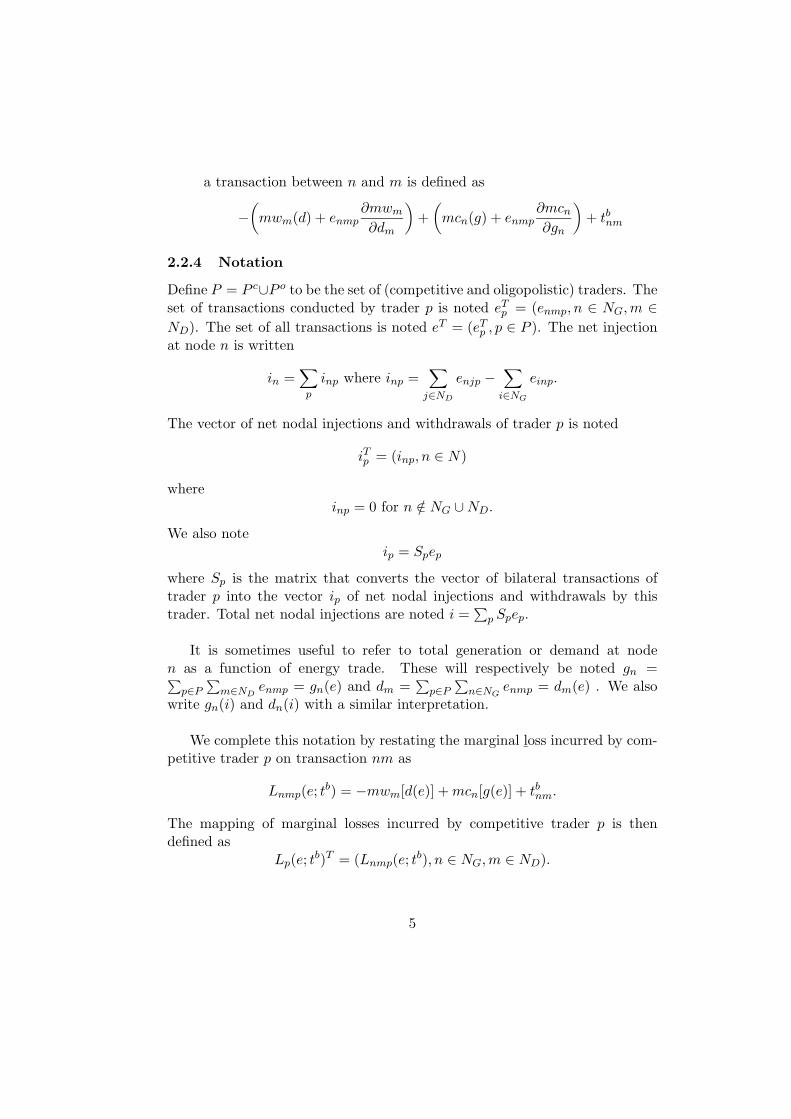
2.2.4 Notation

Define P = P c∪P o to be the set of (competitive and oligopolistic) traders. Theset of transactions conducted by trader p is noted eT

p = (enmp, n ∈ NG, m ∈ND). The set of all transactions is noted eT = (eT

p , p ∈ P ). The net injectionat node n is written

in =∑p

inp where inp =∑

j∈ND

enjp −∑

i∈NG

einp.

The vector of net nodal injections and withdrawals of trader p is noted

iTp = (inp, n ∈ N)

whereinp = 0 for n /∈ NG ∪ ND.

We also noteip = Spep

where Sp is the matrix that converts the vector of bilateral transactions oftrader p into the vector ip of net nodal injections and withdrawals by thistrader. Total net nodal injections are noted i =

∑p Spep.

It is sometimes useful to refer to total generation or demand at noden as a function of energy trade. These will respectively be noted gn =∑

p∈P

∑m∈ND

enmp = gn(e) and dm =∑

p∈P

∑n∈NG

enmp = dm(e) . We alsowrite gn(i) and dn(i) with a similar interpretation.

We complete this notation by restating the marginal loss incurred by com-petitive trader p on transaction nm as

Lnmp(e; tb) = −mwm[d(e)] + mcn[g(e)] + tbnm.

The mapping of marginal losses incurred by competitive trader p is thendefined as

Lp(e; tb)T = (Lnmp(e; tb), n ∈ NG, m ∈ ND).

5

Similarly the marginal loss of oligopolistic trader p on transaction nm is re-formulated as

Lnmp(e; tb) = −(mwm[d(e)] + enmp

∂mwm∂dm

|d(e)

)

+(mcn[g(e)] + enmp

∂mcn∂gn

|g(e)

)+ tbnm

and the mapping of the marginal losses incurred by trader p is defined as

Lp(e; tb)T = (Lnmp(e; tb), n ∈ NG, m ∈ ND).

3 Bilateral models of restructured electricity sys-tems

3.1 There are no transmission constraints

3.1.1 The equilibrium

Definitions. An equilibrium without transmission constraints is a pair ofvectors (g∗, d∗, e∗), π∗ = (π∗

n, n ∈ N) such that

- g∗n maximises the profit of generator n at price π∗n, n ∈ NG

(this implies π∗n = mcn(g∗) when g∗n > 0 and π∗

n ≤ mcn(g∗) when g∗n = 0)

- d∗m maximises the surplus of consumer m at price π∗m, m ∈ ND

(this implies π∗m = mwm(d∗) when d∗m > 0 and π∗

m ≥ mwm(d∗) whend∗m = 0)

- e∗p maximises the profit of competitive trader p at the price π∗

- e∗p maximises the profit of oligopolistic trader p, given the transactionse∗−p = (e∗p′ , p

′ ∈ P, p′ = p) of the other traders, p ∈ P o.

A competitive equilibrium without transmission constraints is an equilib-rium without transmission constraints where oligopolistic traders are inactive(e∗p = 0, p ∈ P o) or do not exert market power ( ∂

∂dmmwm(d∗) = ∂

∂gnmcn(g∗) =

0).

The prices π∗ are commonly referred to as the nodal prices of electricity.

6

3.1.2 Computation

In order to compute this equilibrium we introduce the variational inequalityproblem

V I1: Seek e∗ ≥ 0 such that∑p∈P

Lp(e∗; tb)T (ep − e∗p) ≥ 0 for all ep ≥ 0.

3.1.3 Properties

Assumption. We impose the following assumptions already introduced inMurphy et al (1983):

· for all m, the revenue function [mwm(enm + K)]enm obtained by sellingenergy to consumer m is concave in enm ∀ K > 0;

· for all n, the procurement cost function [mcn(enm + K)]enm obtained bybuying energy from the generator n is convex in enm ∀ K > 0.

This assumption guarantees the monotonicity of the mappings Lp (seeHarker and Pang (1990) for a definition of monotonicity). Recall that strictmonotonicity is equivalent to coercivity when case mwm and mcn are affine.The following propositions can then be established.

Proposition 1 Assume Lp(e; tb) is monotone and coercive for all p ∈ P ,then V I1 has a compact convex, non empty solution set. If Lp(e; tb) is strictlymonotone, the solution is unique.

Proposition 2 A solution to V I1 is an equilibrium of the bilateral modelwithout transmission constraint.

Proposition 3 If competitive traders can engage in the same bilateral trans-actions as oligopolistic traders, then the equilibrium is competitive.

3.1.4 Discussion

An obvious question is whether it makes sense to compute equilibria withouttransmission constraints ? This may look doubtful in theory but is relevantin practice. Specifically the constraints imposed by the network have longbeen ignored explicitly or implicitly by many both in Europe and the US.A commonly heard claim is that the network is overbuild and transmission

7

constraints are irrelevant (Boucher et al (1998)). The contract path approachwhich is so common in transmission practice implicitly neglects transmissionconstraints (see Harvey et al (1997) for an extensive discussion of the subject).Also barter deals were commonly used in the old regulatory days to handleoccasional congestion at border between control areas. It is sometimes sug-gested that they can still be used to remedy transmission constraints in therestructured industry (EC Energy Monthly (1999) reports that the EuropeanCommission helds such a position). In brief transmission constraints are oftenthought to be irrelevant.

The fallacy of both the diagnostic and the remedy is progressively realized,but the full consequences of network constraints are not for that matter fullytaken into consideration. It is indeed sometimes stated that is suffices to pre-vent access to the network when transmission capacity is limited. The onlyrequirement to fulfill would be that this restriction be non discriminatory. Asargued below achieving non discriminatory restriction in access without prop-erly pricing network constraints may be an impossible task in practice. In orderto discuss this point we first introduce a bilateral model where transmissionconstraints are explicitly recognised, even though no market for transmissionservices is introduced.

3.2 There are transmission constraints but no market for trans-mission services

The following notation will be useful to state the problem. We redefine thenetwork capacity NC as NCb (network capacity in the bilateral representa-tion) to make the reference to bilateral transactions explicit

NCb ≡ {e | e ≥ 0,∑p

ΓSpep ≤ f}.

The residual network capacity NCbp(e−p) (network capacity available to p when

e−p is given) can then be defined as

{ep | ep ≥ 0,ΓSpep +∑p′ �=p

ΓSp′ ep′ ≤ f}.

3.2.1 The equilibrium

It is possible to analyse the equilibria achievable when there are transmissionconstraints but no market for transmission services by resorting to the notion

8

of generalized equilibrium (Rosen (1965)). Specifically

Definitions. A generalized equilibrium is a pair of vectors (g∗, d∗, e∗), π∗ suchthat

- g∗n maximises the profit of generator n at price π∗n, n ∈ NG

- d∗m maximises the surplus of consumer m at price π∗m, m ∈ ND

- e∗p maximises the profit of competitive trader p at the price π∗, given thenetwork capacity NCb

p(e∗−p) available to p when the transactions e∗−p are

given

- e∗p maximises the profit of oligopolistic trader p, given the transactions e∗−p ofthe other power marketers and the residual network capacity NCb

p(e∗−p)

available to p as a result of these transactions.

A social equilibrium (Debreu (1952)) is a generalised equilibrium where oligo-polistic traders are inactive or cannot exert market power.

3.2.2 Computation

Define the following quasi variational inequality problem (see Chan and Pang(1989))

QV I: Seek e∗ ∈ NCb such that∑p∈P

Lp(e∗; tb)T (ep − e∗p) ≥ 0 for all ep ∈ NCbp(e

∗−p).

3.2.3 Properties

Proposition 4 Assume Lp(e; tb) is monotone. QVI has a solution but it willgenerally not be unique.

Proposition 5 A solution to QVI is a generalised equilibrium.

Proposition 6 Suppose that competitive traders can engage in the same trans-actions as oligopolistic traders. Then both competitive and oligopolistic traderscan be active on the same markets.

9

3.2.4 Discussion

The relevance of the generalised equilibrium, and hence of the associated QV Iproblem has been introduced above by referring to general attitudes with re-spect to network constraints. Various developments both in the theoreticalliterature and in the restructuring practice provide additional ground to thisjustification. The importance of tradable transmission rights and of a marketfor transmission rights in restructured electricity systems has been extensivelydebated by Oren (1997) and Stoft (1999). It is impossible to do justice to thisdiscussion in a few lines here. It suffices to say that the absence of a marketfor transmission markets creates a fundamental indeterminacy in the outcomeof the energy market and that this uncertainty can exacerbate the marketpower of some of the agents. Generalised equilibria might thus be a very rel-evant concept for analysing systems designed without markets for transmissionrights. In practice markets for transmission rights are introduced in many sys-tems in the US (PJM, California, NEPOOL, ...) while EU documents do notseem to mention them. An other illustration of the relevance of generalisedequilibria can be found in the discussion of Harvey et al (1997), Oren et al(1995) and Wu et al (1996) relative to the definition and uniqueness of theequilibrium in restructured electricity systems.

Because of the importance given to non discriminatory access to the net-work both in the EU and the US, we believe that the following proposition maycontribute to further justify analysing equilibria without markets for trans-mission services in case these are effectively implemented in practice. Theproposition is stated in this section and discussed in more detail later on.

Proposition 7 Markets without tradable transmission rights lead to implicitdiscriminatory access prices.

3.3 The equilibrium when there are network constraints anda market for transmission services

3.3.1 Computation

Consider the following variational inequality problems

V I2: Seek e∗ ∈ NCb such that∑p∈P Lp(e∗; tb)T (ep − e∗p) ≥ 0 for all e ∈ NCb

10

or equivalently (see for instance Harker and Pang (1990) for the proof of theequivalence.)

V I2 : Seek e∗ ∈ NCb, λ∗ ≥ 0 such that∑p∈P [Lp(e∗; tb) + λ∗Γ

∑p Sp]

T (ep − e∗p) + (f − Γ∑

p Spe∗p)

T

(λ − λ∗) ≥ 0 for all e ∈ NCb, λ ≥ 0

where, for a solution λ∗ of V I2, e∗ also solves

˜V I2: Seek e∗p ≥ 0 such that∑

p∈P (Lp(e∗; tb) + λ∗ΓSp)T (ep − e∗p) ≥ 0 for all ep ≥ 0.

3.3.2 Congestion charges

Let (e∗, λ∗) be a solution of V I2. λ∗ΓSp defines congestion charges which canbe given different interpretations

(i) λ∗� , � ∈ L is the congestion charge on line �, � ∈ L (Chao and Peck (1996),(1997), (1998), Wilson (1997)). In this interpretation traders pay for theutilisation of the lines. This utilisation is computed from their energytransactions using the distribution factors of the Γ matrix. λ∗

� is the unitprice for the utilisation of line �.

(ii) λ∗Γ = τ∗ is the vector of nodal charge to withdraw/inject at node n(Schweppe et al (1988), Hogan (1992)) . In this interpretation, traderspay for the right to inject and withdraw electricity. −τ∗

n and +τ∗n are

respectively the charges to inject and withdraw at node n. The totalinjection and withdrawal services required by trader p are given by Spep.

(iii) λ∗ΓSp = ε∗ where ε∗nm is the bilateral charge between n and m (Schweppeet al (1986), Hogan (1992)). In this interpretation traders pay for a pairof injection and withdrawal rights. Note that ε∗nm = τ∗

m−τ∗n. The vector

of transmission services required by trader p is given by ep.

Setting tb = ε∗ = +λ∗ΓSp, it is easy to see that ˜V I2 becomes the Vari-

ational Inequality problem associated to a bilateral market without transmis-sion constraints but where transmission charges are given by ε∗, namely

V I1: Seek e∗ ≥ 0 such that∑p∈P Lp(e∗; ε∗)T (ep − e∗p) ≥ 0 for all ep ≥ 0.

11

3.3.3 Discussion

The relation between the solution to QV I and V I2 is easily established fromthe following result which is a direct adaptation of Theorem 4 in Harker (1991).

Lemma 1 e∗ is a solution to QV I iff there exists λ∗p, p ∈ P such that

e∗, (λ∗p, p ∈ P ) is a solution to the following VI problem.

V I: Seek e∗ ≥ 0, λ∗p ≥ 0, p ∈ P such that∑

p∈P

[Lp(e∗; tb)T + λ∗

pΓSp

](ep − e∗p) +

∑p∈P (f − Γ

∑p′ Sp′e

∗p′)

(λp − λ∗p) ≥ 0 for all e ≥ 0, λp ≥ 0, p ∈ P .

This lemma shows that a solution to QV I can be interpreted as an equi-librium of the bilateral market without transmission constraints where powermarketers are charged (possibly) different transmission levies ε∗p = λ∗

pΓSp. Inbrief a generalised equilibrium is an equilibrium without transmission con-straints where access to the network is priced in a discriminatory way exceptfor some very special cases. This special case which corresponds to non dis-criminatory access pricing is characterised in Lemma ??.

Lemma 2 A solution e∗ to QV I is a solution to V I2 iff λ∗p = λ∗ for all p.

This lemma is an adaptation of Theorem 6 in Harker (1991). It fullycharacterises the relationship between solutions to QV I and V I2.

3.3.4 The equilibrium

The following property generalises results found in Hogan (1992) and Chaoand Peck (1996)) to the oligopolistic case.

Proposition 8 Let e∗ be a solution to V I2 and i∗ and f∗ the correspondingnet injections and flows. Let ε∗, τ∗ and λ∗ be defined as before. Then thefollowing holds

(i) e∗ maximises∑

p ε∗pep s.t. ep ≥ 0,Γ∑

p Spep ≤ f

(ii) i∗ maximises τ∗ ∑p i∗p s.t. Γ

∑p ip ≤ f

(iii) f∗ maximises λ∗�f� s.t. f� ≤ f �.

12

Properties (i) and (ii) can be interpreted as the behaviour of an ISO whichsells transmission rights so as to maximise the value of the network. Not-withstanding its monopoly position, this ISO is supposed to take the price ofthese services as given. This interpretation is advocated by Hogan(1992) andHarvey et al (1997). Property (iii) can be interpreted as the behaviour of aline owner that tries to maximise the value accruing from selling line services.This line owner also takes prices as given. This interpretation is advocated byChao and Peck (1996), (1997).Using Proposition ?? the following alternative definitions of equilibria can bestated.

Definitions. An equilibrium of the energy and transmission service marketsis a pair of vectors (g∗, d∗, e∗), (π∗, λ∗

p, p ∈ P ) such that

(i) there is equilibrium on the energy market in the sense introduced below,

(ii) there is equilibrium on the transmission service market in one of theinterpretations introduced below.

The energy market. (g∗, d∗, e∗)(π∗, λ∗p, p ∈ P ) is an equilibrium on the

energy market iff

- g∗n maximises the profit of generator n at price π∗n, n ∈ NG

- d∗m maximises the surplus of consumer m at price π∗m, m ∈ ND

- e∗p maximises the profit of the competitive trader p at the price π∗, giventhe bilateral transmission charges t∗p = +λ∗

pΓSp

- e∗p maximises the profit of oligopolistic trader p, given the transactions e∗−p

of the other traders and the transmission charges t∗p = +λ∗pΓSp.

The transmission market. (e∗p, λ∗p), p ∈ P is an equilibrium on the trans-

mission service market iff any one of the following alternative definitions holds

- λ∗p(f − Γ

∑p Spe

∗p) = 0 and λ∗

p = λ∗ ≥ 0 ∀p (traders exchange bilateraltransmission rights on a bilateral market (Boucher and Smeers (1999))

- λ∗p = λ∗ ≥ 0 ∀p and e∗ maximises

∑p(λ

∗ΓSp)ep | ep ≥ 0,Γ∑

p Spep ≤ f (theISO maximises the value accruing from sales of bilateral transmissionrights compatible with the network capacity (Hogan (1992))

- λ∗p = λ∗ ≥ 0 ∀p and i∗p = Spe

∗p maximises

∑p λ∗Γip | Γ

∑p ip ≤ f (the ISO

maximises the value accruing from the sales of nodal transmission rightscompatible with the network capacity (Hogan (1992))

13

- λ∗p = λ∗ ≥ 0 ∀ p and f∗

� = Γ∑

p Spe∗p maximises λ∗

�f� | f� ≤ f � for all �(line owners maximise the value of their assets by selling line utilisationservices (Chao and Peck(1996)).

The relation between these definitions is established through the followingproposition.

Proposition 9 All definitions of equilibria are equivalent.

Proposition 10 An equilibrium of the energy and transmission service mar-ket is a generalised equilibrium where congestion charges are priced in a nondiscriminatory way.

Finally Proposition ?? relates the preceding material to the usual char-acterisation of nodal prices in competitive electricity market (Schweppe et al(1988), Hogan (1992)). Specifically transmission prices are in these conditionsdirectly derived from nodal electricity prices.

Proposition 11 Suppose that there is no oligopolistic traders or that they areinactive, then τ∗ = −π∗.

4 Alternative organisations of the market

4.1 Preliminaries: nodal and bilateral models

A nodal representation of the bilateral model can easily be obtained usingthe notion of balanced schedules. Let u = (1, 1, . . . , 1) be a vector of dimen-sion equal to the number of nodes. Because losses are neglected, the vectorof net injection of trader p, ip = Spep satisfies uip = 0. By definition ip is abalanced schedule. This notion has played a key role in the Californian reform.

In order to proceed towards the nodal reformulation of the bilateral modelwe first rewrite the marginal loss mappings Lp(e; t) in terms of net injections.As a preliminary replace the vector tb of bilateral transmission charges by avector tno = (tno

n , n ∈ N) of nodal transmission charges. Marginal losses canthen be introduced as follows.

Lnp(i; tno) = −mwn(d(i)) + tnon , n ∈ ND, and

Lnp(i; tno) = mc(g(i)) + tnon , n ∈ NG,

14

are respectively the marginal losses due to a withdrawal and injection of com-petitive trader p ∈ P c at node n.

Similarly,

Lnp(i; tno) = −(mwn(d(i)) + inp

∂mwn∂dn

)+ tno

n , n ∈ ND, and

Lnp(i; tno) =(mcn(g(i)) + inp

∂mcn∂gn

)+ tno

n , n ∈ NG

are respectively the marginal losses due to a withdrawal and injection of theoligopolistic traders p ∈ P 0 at node n.

Finally,Lp(i; tno)T = (Lnp(i; tno), n ∈ N)

is the mapping of nodal marginal losses of trader p.

Using this notation, the bilateral models introduced in Section 3 can becast in terms of balanced schedules. We accordingly state the following prob-lems

No transmission constraint

V Ino1 : Seek i∗, ui∗p = 0, p ∈ P , such that∑

p∈P Lp(i∗; tno)(ip − i∗p) ≥ 0 for all i such that uip = 0, p ∈ P.

Transmission constraints but no market for transmission services

Define the residual network capacity NCnop (i−p) ≡ {ip | Γip +

∑p′ �=p Γip′ ≤ f}

QV Ino: Seek i∗ ∈ NC, ui∗p = 0, p ∈ P such that∑p∈P Lp(i∗; tno)(ip − i∗p) ≥ 0 for all i such that uip = 0 and

ip ∈ NCnop (i∗−p).

Transmission constraints and market for transmission services

V Ino2 : Seek i∗ ∈ NCno, ui∗p = 0, p ∈ P , such that∑

p∈P Lp(i∗; tno)(ip − i∗p) ≥ 0 for all i such that uip = 0 andi ∈ NC.

Properties stated in Section 3 carry through with straightforward adapt-ations to these nodal formulations. Taking stock of these formulations, weintroduce a first pool model.

15

4.2 A first pool model

In order to define a Pool, we concentrate on the particular situation wherethere is a single competitive trader hereafter noted c (P c = {c}). Considerthe problem

V Ino2 : Seek i∗ ∈ NCno, ui∗p = 0, p ∈ P such that∑

p∈P Lp(i∗; tno)(ip − i∗p) ≥ 0 for all i such that uip = 0, p ∈ Pand i ∈ NC

V Ino2 is equivalent to

V Ino

2 : Seek i∗, ui∗p = 0 for p ∈ P , λ∗ ≥ 0 such that∑p∈P [(Lp(i∗; tno) + λ∗Γ]T (ip − i∗p) + (f − Γi∗)T (λ − λ∗) ≥ 0

for all i, uip = 0 for p ∈ P , λ ≥ 0.

A solution i∗, λ∗ of V Ino

2 is also a solution of the two following problems

˜V I

no

2,c:

˜V I

no

2,P o :

Seek i∗c , ui∗c = 0 such that[Lc(i∗; tno) + λ∗Γ]T (ic − i∗c) ≥ 0 for all ic, uic = 0

Seek i∗p, ui∗p = 0 for p ∈ P o, such that∑p∈P 0 [Lp(i∗; tno)+λ∗Γ]T (ip−i∗p) ≥ 0 for all ip, uip = 0, p ∈ P o.

Problem ˜V I

no

2,c describes the behaviour of the competitive trader. As before,note τ∗ = λ∗Γ and define π∗ as a vector of nodal prices that satisfy thefollowing complementary slackness conditions (see section ??).

π∗n − mcn(g(i∗)) ≤ 0 and [π∗

n − mcn(g(i∗))]gn(i∗) = 0, n ∈ NG

−π∗n + mwn(d(i∗)) ≤ 0 and [−π∗

n + mwn(d(i∗))]d(i∗) = 0, n ∈ ND

It is easy to see from the statement of problem ˜V I

no

2,c that π∗ = τ∗+β∗c (where

β∗o is the dual variable of the constraint uic = 0 at the solution i∗c) satisfies

these complementary slackness conditions and hence defines a set of nodalprices in the sense of Schweppe et al (1988), Hogan (1992) and many others.Also, transmission between two nodes is priced at a level equal to the differ-ence between τ∗

n and hence also between nodal prices π∗n.

These two properties (the existence of nodal prices and the above relationbetween transmission and nodal prices) characterise a pool. They are satisfiedby the solution to problem V Ino

2 . To see that they are not satisfied in general,

16

consider problem ˜V I

no

2,P when there is no competitive trader. The equilibriumconditions associated to an oligopolistic trader active at nodes n and m (i∗np >0 and i∗mp < 0) can be stated as

mcn(g∗) + i∗np∂mcn∂gn

= τ∗n + β∗

p n ∈ NC

mwm(d∗) + i∗mp∂mwm∂dm

= τ∗m + β∗

p m ∈ ND

where β∗p is the dual variable of the balance schedule constraint uip = 0.

Transmission between nodes n and m is priced at

τ∗m − τ∗

n = +mwm(d∗) − mcn(g∗) − i∗np∂mcn∂gn

+ i∗mp∂mwm∂dm

< mwm(d∗) − mcn(g∗).

In conclusion a pure oligopolistic market does not satisfy the pool conditions.

The preceding discussion suggests that it suffices to have a competitivetrader accessing all generators and consumers to make the system equivalentto a pool. This result is not satisfactory though. Indeed Proposition 3 tells usthat a competitive trader makes the system not only a pool by also a competit-ive market. In fact, the competitive trader drives the oligopolistic traders outof the market. Because pools are generally not exempt from market power (seeall the theory of supply curve equilibrium) in practice, it would be interestingto be able to model pools that are not perfectly competitive. A first result inthis direction is achieved by assuming that the competitive trader(s) do(es) notaccess the same generators and consumers as the oligopolistic traders. Nodalprices would then be derived from supply and willingness to pay functions ofthose generators and consumers trading through the competitive marketer(s)while oligopolistic traders would have access to other agents and hence wouldsee different supply and willingness to pay functions. The reasoning leadingto Proposition ?? would no longer hold and we would have a pool which is notcompetitive. Such a situation would be achieved in practice if one were to as-sume that small generators and consumers (or their representative distributioncompanies) trade through the pool while large generators and consumers tradevia bilateral contracts. This system satisfies the property of a pool where nodalprices are determined by the prices paid to and by these small generators andconsumers. In this system nodal prices also determine the transmission pricespaid by the bilateral transaction that take place outside the pool. Such mixedsystems satisfy the definition of a pool and are indeed found in practice. Theirmathematical definition remains unsatisfactory though as it requires that the

17

modeler identifies the generation and consumption segments of the marketthat trade through the pool and those which do not, a dauting task indeed. Amore useful construction of a pool is in order. It has recently been provided byHobbs (1999). Hobbs model was formulated as a complementarity problem.The following presentation is cast in our variational inequality context.

Before leaving this section, note that a two stage version of the above modelhas been introduced in Hogan (1997). Our one stage version is mathematicallymuch simpler. Whether it is or not more realistic than the two stage modelin an empirical question that is not discussed here.

4.3 A Cournot pool model

4.3.1 Hobb’s artibrageur

Consider again the particular case where there is a single competitive traderh hereafter refered to as Hobbs’ trader or the arbitrageur (P c = {h}). Sup-pose P c and P o cover the same markets. Suppose that the market functionsaccording to a two stage structure similar to Hogan (1997)). In the first stage,oligopolistic traders trade a la Cournot knowing that there is a second stage.In this latter, the Hobb’s trader arbitrages between nodes to take advantage ofdifferences between nodal prices and transmission charges. As seen in section??, transmission charges in an oligopolistic market are indeed smaller thandifferences between nodal prices. This creates an opportunity for profit thatthe arbitrageur takes advantage of. The end result of Hobb’s trader activityis that the difference of nodal prices between two arbitrary nodes at the equi-librium of the second stage game is always equal to the transmission chargebetween these nodes. This satisfies the characteristic of a pool as all bilat-eral transactions pay transmission prices equal to difference of nodal prices.Needless to say oligopolistic traders loose some of their market power in theprocess as they can no longer (price) discriminate between generators and cus-tomers. In contrast with the result of the preceding section, the oligopolisticand the arbitrageur can both operate on the same segments of the marketwithout making the market purely competitive. The main differences (and amathematically essential one) between this model and the one of section ??is that these traders do not operate in the same stage of the market. We nowexplore this process in more details.

18

4.3.2 A two stage equilibrium approach

The preceding discussion can be formalised as an equilibrium problem sub-ject to equilibrium constraints. The following characterises the second stageequilibrium. For the sake of simplification we drop all references to tno in therest of this section. We also write i = (iP o , ih) where iP o = (ip, p ∈ P o) todistinguish between the injection of the oligopolistic traders and those of thearbitrageur.

Second stage problem of Hobbs’ trader

- Let (i∗p, p ∈ P o) be given from the first stage. Trader h solves the problem:

Seek i∗h, ui∗h = 0 such that [Lh(i∗P o , i∗h) + τ∗] (ih− i∗h) ≥ 0 for all ih, uih =0.

- Suppose that Lc is affine and coercive in ih. This variational inequalityproblem has a unique solution ih(iP o) which is itself an affine functionof iP o . It is the solution of the affine system of equations

Lh(iP o , ih) + τ∗ + βh = 0, uih = 0 where (βh(balance) is the dual variableof uih = 0.

In order to move from the second to the first stage, one needs to model theassumption that trader p ∈ P o takes the reaction ih(ioP ) of the arbitrageurinto account in the first stage. This is done as follows.

First stage problem of an oligopolistic trader

Consider a trader p ∈ P o. Note P o/p the set of oligopolistic traders dif-ferent from p and define Lo and La (respectively o for oligopolistic, a forarbitrage) the respective contributions to the marginal loss of trader p fromhis/her action (inp) and from the arbitrageur’s actions (inh):

Lonp = −

(mwn(d(i)) + inp

∂mwn∂inp

), La

np = −inp∂mvn∂inh

if n ∈ ND

Lonp = mcn(g(i)) + inp

∂mcn∂inp

, Lanp = inp

∂mcn∂inh

if n ∈ NG

Trader p ∈ P o then solves the problem:

Seek i∗p, i∗h, ui∗p = 0, ui∗h = 0 and L(i

∗p, i

∗P o/p, i

∗h) + τ∗ + β∗

h = 0 such that[Lo

p(i∗p, i

∗P o/p, i

∗h) + τ∗

]T(ip−i∗p)+

[La

p(i∗p, i

∗P o/p, i

∗h)

]T(ih−i∗h) ≥ 0 for all ip, ih, uip =

0, uih = 0 and Lh(ip, i∗P o/p, ih) + τ∗ + β = 0.

19

An equivalent first stage problem

Combining the behaviour of all traders, we state the following variationalinequality problem.

V Ipool : Seek i∗P o , i∗h, λ∗ ≥ 0 satisfying ui∗p = 0, p ∈ P o, ui∗h = 0,(i∗P o , i∗h) ∈ NC, Lh(i∗P o , i∗h) + λ∗Γ + β∗

h = 0 such that∑p∈P o

{[Lo

p(i∗P o , i∗h) + λ∗Γ]T (ip − i∗p)

+[Lap(i

∗P o , i∗h)]T (ih − i∗h)]

}+[f − λ∗Γ(

∑p∈P o∪{h} i∗p)]

T (λ − λ∗) ≥ 0for all λ ≥ 0 and iP o , ih, satisfying uip = 0, p ∈ P o, uih = 0,Lh(iP o , ih) + λΓ + β0 = 0.

Proposition 12 Suppose the mappings Lop, La

p, p ∈ P o are monotone andcoercive and Lc is affine and coercive, then V Ipool has a single solution. Thissolution is a Pool with Cournot players in the sense of Hobbs.

4.4 The pool and bilateral models

The relation between the bilateral and pool organisations of the market re-ceived considerable attention in the literature. The discussion probably peakedat the time of the restructuring in California. The general conclusion of thisdiscussion is that the two systems are equivalent when there is no marketpower. To the best of our knowledge this conclusion was never proved form-ally and no analysis of the relation between the two systems is available for thecase where there is market power. This subsection takes stock of the preced-ing variational inequality formulations to formally establish the equivalencebetween the Pool and the bilateral model when there is no market power.It also establishes that this equivalence does not hold when there is marketpower. This is stated in the following proposition.

Proposition 13 The bilateral and pool models are equivalent when there isno market power. They are not equivalent when there is market power.

The following proposition was first hinted in Smeers and Wei (1997). Itgeneralises a standard result of imperfect competition to the case of electricitymarkets with transmission constraints.

20

Proposition 14 The bilateral and pool models can be made almost equival-ent, and almost equivalent to the competitive equilibrium when the number ofoligopolistic traders is large enough.

5 Regulated transmission markets

5.1 Infrastrusture costs: background

Congestion charges are due to limitations of transmission capacities. It iscommonly admitted that congestion charges do not provide revenue sufficientto cover infrastructure costs. These latter, or their fraction not covered bycongestion charges, must then be recovered through other levies.

A wide variety of charges have been introduced (access charge, networkservices ...) to recover infrastructure costs. A natural question is whether onecan tackle both congestion and these other charges in a single computationalframework. The answer is that computational models can still be devised eventhough solution existence and uniqueness become much more difficult if notimpossible to establish on a simple basis.

For the sake of simplification in this presentation, we assume a single net-work service charge collected through a postage stamp, that is a uniform, perKwh, charge.

5.2 Separate congestion and network service charges

5.2.1 Computation

The following model considers the situations where two types of charges arerecovered from the user of the network (here the power marketers). The firstcharge is the standard congestion charge discussed in the preceding sections.The second levy is a postage stamp which is supposed to cover the revenuerequirement of the network. Altogether, these charges add up to more thanthe total costs incurred by the transmission activity. This decomposition ofcharges is common. It can be found, for instance, in Eurelectric (1998) wherenetwork infrastructure costs and measures for dealing with congestion are in-deed seen as two separate matters. This model is constructed on the basis ofthe nodal version of the equilibrium problem.

Consider the nodal model where we initially assume tno = 0.

21

V Ino2 : Seek i∗ ∈ NCno, ui∗p = 0, p ∈ P , such that∑

p∈P Lp(i∗; 0)(ip − i∗p) ≥ 0 for all i such that uip = 0 andi ∈ NCno

Let RRN be the (revenue requirement of the network) to be collectedthrough a postage stamp ts (a unique charge independent of the node). It isassumed that this postage stamp is only charged at the consumption sites. Thecovering of the revenue requirement is expressed by the constraintts

∑n∈ND

∑p inp = −NNR (recall inp ≤ 0 for n ∈ ND). Introducing this

constraint in V Ino2 leads to the following mixed variational inequality problem.

MV I: Seek i∗ ∈ NCn, t∗s, ui∗p = 0, p ∈ P such that∑p∈P [Lp(i∗; ts∗)]T (ip−i∗p) ≥ 0 for all i such that uip = 0, p ∈ P ,

and i ∈ NCno and ts∗∑

n∈ND

∑p i∗np = −NNR.

5.2.2 The equilibrium

Transmission charges at some node thus consist of two parts: ts∗ which is onlycollected (in this version of the model) at the demand node and τ∗

n which isthe congestion charge. The definitions of the equilibrium presented in section3 are readily adapted to this new context. We only mention the adaptation tothe case where the ISO maximises the revenue accruing from nodal congestioncharges.

Definition. An equilibrium of the energy and transmission service marketswith coverage of infrastructure cost is a pair of vectors (g∗, d∗, i∗), (π∗, λ∗, ts∗)such that

(i) there is equilibrium on the energy market in the sense introduced below

(ii) there is equilibrium on the transmission service market in the sense in-troduced below

The energy market (g∗, d∗, e∗)(π∗, λ∗, t∗) is an equilibrium on the energymarket iff

- g∗n maximises the profit of generator n at price π∗n, n ∈ NG

- d∗m maximises the profit of consumer m at price π∗m, m ∈ ND

- i∗p maximises the profit of the competitive trader p at the price π∗, giventhe nodal transmission charges τ∗ = λ∗Γ and the infrastructure chargets∗

22

- i∗p maximises the profit of oligopolistic trader p, given the transactions e∗−p

of the other traders, the nodal transmission charges τ∗ = λ∗Γ and theinfrastructure charge ts∗.

Transmission market (i∗p, τ∗, ts∗) is an equilibrium on the transmission

service market iff the following holds

- i∗ maximises {τ∗ ∑p ip | Γ

∑p ip ≤ f} (the ISO maximises the value accruing

from the sales of nodal transmission rights compatible with the networkcapacity)

- ts∗∑

n∈ND

∑p i∗np ≥ −NNR (the infrastructure costs are covered).

The existence and uniqueness of this equilibrium are established throughthe following proposition. The proof of this proposition follows from notingthat ts∗

∑n∈ND

∑p i∗np = −NNR can be replaced by ts∗(−∑

n∈ND

∑p i∗np) ≥

NNR which defines a convex set.

Proposition 15 Suppose that the loss mappings are monotone and coercive.Then the solution to MVI exists and is unique. It is also an equilibrium in theabove sense.

5.3 Nodal and zonal systems

5.3.1 Background

Distinguishing electricity prices on a nodal basis is not a readily accepted idea.The common wisdom has been for a long time that nodal systems are too com-plex to be implemented in practice (even though they were already operatingin some countries). This attitude prevailed in the early days in the US andthe issue is still heavily debated today. This belief is certainly the rule inEurope as no nodal system is envisaged at this stage on the continent. Zonalprices have been proposed as an alternative to nodal prices. By definitionzonal pricing associates prices, not to individual nodes but to zones of nodes.The limit case of the zonal system is the single node zone or nodal system.

The following shows that the variational inequality framework allows oneto model zonal systems. As an example we consider the case where conges-tion is charged according to a zonal pattern and no other charge (such asinfrastructure cost) is recovered. At least two approaches can be envisagedfor zonal prices. The first one consists of distributing zonal congestion coststhrough each zone. In the second approach the ISO engages is countertrading

23

and distributes the cost accruing from this countertrading activity. We limitourselves to the first case.

5.3.2 The equilibruim

The definition of the equilibrium associated to the solution of this variationalinequality problem is readily derived from the bilateral equilibria discussed insection 3. An illustration of this type of adaptation is given in section ??. Thesame procedure applies here.

5.3.3 Computation

Consider a partitioning N = ∪z∈ZNz (z for zones) of the nodes into zones.Zonal charges are obtained by perturbing nodal prices so as to make all nodalprices in a zone equal. Zonal charges should also cover congestion cost in eachzone. We achieve both requirements by appropriately choosing the additionalnodal charge tno

n . Consider the nodal problem V Ino2 .

V Ino2 : Seek i∗ ∈ NC, ui∗p = 0, p ∈ P such that∑

p∈P Lp[(i∗; tno)](ip−i∗p) ≥ 0 for all i such that uip = 0, p ∈ P ,and i ∈ NCno

At equilibrium i∗ solves the problem

˜V I

no

2 : Seek i∗, ui∗p = 0, p ∈ P such that∑p∈P [Lp(i∗; tno) + λ∗Γ](ip − i∗p) ≥ 0 for all i such that uip =

0, p ∈ P .

A zonal pricing scheme is achieved for a tno∗ such that

(i) tno∗n + (λ∗Γ)n = atno∗

z (where atnoz stands for average nodal transmission

charge) for all nodes n, n ∈ Nz, and

(ii) atno∗z

∑n∈Nz

∑p i∗np =

∑n∈Nz

(λ∗Γ)n(∑

p i∗np) (all congestion charges arecovered).

Under these conditions all nodal charges in a zone are identical and turnout to be averages of nodal congestion charges.

Define tno = (tnon , n ∈ N) and atno = (atno

z , z ∈ Z). These conditions canbe cast in the following single variational inequality problem

24

V Izo2 : Seek i∗ ∈ NC, ui∗p = 0, p ∈ P , tno∗, atno∗ such that∑

p∈P [Lp(i∗; tno∗)]T (ip − i∗p) +∑

z∈Z

∑n∈Nz

[tno∗n − (λ∗Γ)n −

atno∗z ]T (tno

n −tno∗n )

+∑

z∈Z [atno∗z

∑n∈Nz

i∗n − ∑n∈Nz

(λ∗Γ)ni∗n]T (atnoz − atno∗

z ) ≥ 0for all i ∈ NC, uip = 0, p ∈ P , tno, atno.

While the existence and uniqueness of the solution of the models of Sec-tions 3 and 4 can easily be derived from standard results, this is no longerthe case here. The mapping appearing in problem V Izo does not have anymonotonicity property. Solutions may thus fail to exist or multiple solutionsmay also exist. The algorithmic situation is also much bleaker even thoughprocedures for handling this problem may be found in the literature (and seento be working quite well). Two approaches coming from quite different origins(Dafermos (1983), Greenberg and Murphy (1985)) can be used and lead tosimilar approaches. Specifically both will require to solve the following se-quence of problems

V I2(tno,k): Seek ik∗ ∈ NC, uik∗p = 0, p ∈ P such that∑p∈P Lp(ik∗; tno,k)(ikp − ik∗p ) ≥ 0 for all ik such that uikp =

0, p ∈ P, ik ∈ NC

Update tno,k into tno,k+1 by solving the system

atno,k+1z

∑n∈Nz

ik∗n =∑

n∈Nz(λk∗Γ)nik∗n

tno,k+1n = (λk∗Γ)n + atno,k+1

z .

Convergence conditions for this approach can be found in Dafermos (1983).

6 Numerical results

The following results illustrate the relevance of being able to model alternativemarket designs and to simulate their operation.

We consider a problem with 13 nodes and 21 lines. Four generators arelocated on these nodes. They are supposed to be owned by 4 power marketers.This formulation is slightly different from the one analysed in the paper: firstpower marketers only exert market power towards consumers and not towardsgenerators as they own them. Second two markets segments are located at

25

each node, each represented by a demand curve. In order to illustrate the im-pact of market design, we consider two alternative assumptions of competitionand three alternative regimes of transmission pricing. Specifically we modelthe case where power marketers do not exert market power and the one wherethey behave a la Cournot. As to transmission we successively consider the casewhere congestion charges constitute the only payment for transmission servicesand the one where both congestion charges and the cost of the infrastructureare recovered in a single transmission charge. In this latter case we distinguishthe case where the total transmission charges only cover infrastructure costand the one where they cover the sum of congestion and infrastructure costs.

The following abbreviations summarize the different cases:

per perfect competitionimp imperfect competitionno Nodal PricingZo Inf Single zone, infrastructure coverageZo Inf Co Single zone, infrastructure + congestion

For each run we report numerical results (in Belgian Francs (38BF = 1US$))in term of

Average Electricity AVER PTotal Quantity exchanged TOT QNConsumer’s Utility Function UTILITYTotal Amount received by agents INCOMEVariable Production Costs VARCSTFixed Production Costs FIXCSTTotal Profit of Grid Operator + Agents PROFITGlobal Welfare WLFARE

The results clearly indicate that market design and market power matter alot. This is true wether we consider average prices, total quantities,.... Globalwelfare is the only quantity that is not drastically affected. But its allocationamong agents varies a lot depending on the situation on hand.

26

AV

ER

PT

OT

QN

UT

ILIT

YIN

CO

ME

VA

RC

STF

IXC

STP

RO

FIT

WL

FAR

EM

AR

GIN

Per.

No

1.07

912

4341

.431

1293

805.

353

1298

86.5

4470

220.

208

3628

3.20

823

383.

128

1317

188.

481

0.00

0

Per.

Zo

Inf

1.35

712

1920

.377

1259

807.

459

1204

56.4

1867

982.

617

3628

3.20

816

190.

593

1275

998.

052

0.33

8

Per.

Zo

Inf

Co

1.38

512

1679

.051

1256

463.

220

1196

86.7

7667

756.

232

3628

3.20

815

647.

336

1272

110.

556

0.37

0

Imp.

No

6.01

893

705.

176

7581

77.8

5356

3897

.382

5392

9.93

236

283.

208

4736

84.2

4212

3186

2.09

50.

000

Imp.

Zo

Inf

6.23

192

120.

788

7505

79.7

8557

3972

.784

5241

7.91

736

283.

208

4852

71.6

5912

2585

1.44

40.

266

Per.

Zo

Inf

Co

6.42

290

701.

466

7250

99.1

3458

2501

.355

5106

8.66

836

283.

208

4951

49.4

7912

2024

8.61

30.

496

27

References

[1] Boucher, J. and Y. Smeers (1999). Alternative models of restructuredelectricity systems. Part 1: No market power. Mimeo, CORE, Universitecatholique de Louvain, Louvain-la-Neuve, Belgium.

[2] Boucher, J., Ghilain, B. and Y. Smeers (1998). Security-constrained dis-patch gives financially and economically significant nodal prices. The Elec-tricity Journal, 53–59.

[3] Chan, D. and J.S. Pang (1989). The Generalised quasi-variational in-equality problem. Mathematics of Operations Resarch, 212–222.

[4] Chao, H.-p. and S. Peck (1996). A market mechanism for electric powertransmission. Journal of Regulatory Economics, 10, 25–60.

[5] Chao, H.-p. and S. Peck (1997). An institutional design for an electricitycontract market with central dispatch. Energy Journal, 18(1), 85–110.

[6] Chao, H.-p. and S. Peck (1998). Reliability management in competitiveelectricity markets. Journal of Regulatory Economics, 3, 189–200.

[7] Dafermos, S. (1983). An iterative scheme for variational inequalities.Mathematical Programming, 26, 40–47.

[8] Debreu, G. (1952). A social equilibrium existence theorem. Proceedingsof the National Academy of Sciences U.S.A., 38, 886–893.

[9] EC Energy Monthly (1999). Commission, industry rift over transmissionpricing. Financial Times, 122/9.

[10] Eurelectric (1998). Draft report on national transmission tariffs. Uni-pede/Eurelectric, Brussels, November 18, 1998.

[11] Greenberg, H.J. and F.H. Murphy (1985). Computing regulated marketequilibria with mathematical programming. Operations Research, 35(5),935–955.

[12] Harker Patrick T (1991). Generalized Nash Games and Quasi-VariationalInequalities. European Journal of Operations Research, 54, 81-94.

[13] Harker P. T. and J.S. Pang (1990). Finite-dimensional variational in-equality and non-linear complementarity problems: a survey of theory,algorithm and applications. Mathematical Programming, 48B, 161-220.

28

[14] Harvey, S.M., Hogan, W.W. and S. Pope (1997). Transmission capacityreservations and transmission congestion contracts. Center for Businessand Government, Harvard University, Cambridge (Mass.).

[15] Hobbs, B.F. (1999). Linear complementarity models of Nash Cournotcompetition in bilateral and POOLCO power markets. Submitted toIEEE Transactions on Power Systems, June 1999.

[16] Hogan, W. (1992). Contract networks for electric power transmission.Journal of Regulatory Economics, 4, 211-242.

[17] Hogan, W. (1997). A market power model with strategic interaction inelectricity network. The Energy Journal, 18(4), 107–141.

[18] Hunt, S. and G. Shuttleworth (1996). Competition and choice in electri-city. New York, John and Wiley and Sons.

[19] Murphy, F.H., Sherali, H.D. and A.L. Soyster (1983). Stackelberg-Nash-Cournot equilibria: Characterisation and computation. Operations Re-search, 31(3), 253–276.

[20] Oren, S.S. (1997). Economic inefficiency of passive transmission rightsin congested electricity systems with competitive generation. The EnergyJournal, 18(1), 63–84.

[21] Oren, S.S. (1998). Authority and responsibility of the ISO: objectives,options and tradeoffs. In H.-p. Chao and H.Huntington (eds.), DesigningCompetitive Electricity Markets. Kluwer’s International Series.

[22] Oren, S., Spiller, P. Varariya, P. and F. Wu. Nodal prices and transmissionrights: a critical appraisal. Electricity Journal, 8, 24–35.

[23] Rosen, J.B. (1965). Existence and uniqueness of equilibrium points forconcave n-person game. Econometrica, 33, 520–534.

[24] Schweppe, F.C., Caramanis, M.C. and R.E. Bohm (1986). The costs ofwheeling and optimal wheeling rates. IEEE Transactions on Power Sys-tem, Volume PWRS-1, No. 1.

[25] Schweppe, F.C., Caramanis, M.C. Tabors, R.E. and R.E. Bohn (1988).Spot pricing of electricity. Boston, Kluwer Academic Publishers.

[26] Smeers, Y. and J.-Y. Wei (1997). Do we need a power exchange if thereare enough power marketers. CORE Discussion Paper 9760, Universitecatholique de Louvain, Louvain-la-Neuve, Belgium.

29

[27] Stoft, S. (1999). Financial transmission rights meet Cournot: How TCCScurb market power. The Energy Journal, 20(1), 1–23.

[28] Wu, F. Varaiya, P., Spiller, P. and S. Oren (1996). Folk theorems ontransmission access: Proofs and counterexample. Journal of RegulatoryEconomics, 10(1), 5–24.

[29] Yajima Masajyuki (1997). Deregulatory reforms of the electricity supplyindustry. Quorum books, Westport Connecticut.

30

Notes.

1. Suppose for the three nodes example that plants 1 and 2 are locatedalong a river. Plant 1 is upstream and plant 2 downstream. Supposefurther that both plants are thermal units using the water stream ascold source. The efficienty of each plant and hence its marginal costdepend on the temperature of the stream. While the temperature ofthe water used by unit 1 is unaffected by the operation of plant 2,the converse is not true. Indeed a higher operations level of plant1 increases the temperature of the water used by plant 2. This de-creases the efficiency of plant 2 and hence increases its marginal cost.This externality is modelled by letting the marginal cost of plant 2be a function of both g1 and g2.

2. This allows to represent cross price elasticities between demand atdifferent nodes. This possibility may be relevant to model activityrelocation phenomena.

31

Appendix: Proofs

Proposition 1. The proposition is an adaptation of standard results(e.g. see Harker and Pang (1990)).

Proposition 2. The proof is a special case of the proof of Proposition 9.

Proposition 3. Suppose that pc ∈ P c and po ∈ P o both trade betweennodes n and m, that is e∗nmpc > 0 and e∗nmpo ≥ 0. The solution of V I1

implies

0 = −mwm[d(e∗)] + mcn[g(e∗)] + tbnm (trader pc)0 = −mwm[d(e∗)] + mcn[g(e∗)] + tbnm + e∗nmpo( − ∂mwm

∂dm+ ∂mcn

∂gn) trader po.

Because of the assumption, −∂mw∂dm

and ∂mcn∂gn

are both ≥ 0. Thesecombined wih the two above equalities imply either e∗nmpo = 0 or−∂mwn

∂dm= ∂mcn

∂gn= 0.

Proposition 4. The proof follows from well established results (seeChan and Pang (1989) and/or Harker (1991)).

Proposition 5. The proof follows from well established reasoning (SeeTheorem 4 in Harker (1991) applied in the context of the proof ofProposition 9).

Proposition 6. The following example proves the proposition.

Take a single line network (line 1–2 between nodes 1 and 2). There isone generator of marginal cost 20 + q at node 1 and one consumer ofdemand curve 120 − q at node 2. The capacity of the line is 40. Thereare two power marketers trading between these two nodes. Trader 1 iscompetitive and buys and sells at marginal cost. Trader 2 is oligopolistic.Consider the situation where power marketers 1 and 2 respectively trade30 and 10 between nodes 1 and 2. Nodal prices are respectively 60 and80 at nodes 1 and 2. One easily checks that 30 maximises the profit

(80 − 60)q1 subject to 0 ≤ q1 ≤ 40 − 10

of competitive trader 1 given the residual capacity 30 of line 1–2. Similarly10 maximises the profit

[120 − (30 + q2)]q2 − [20 + (30 + q2)]q2 subject to 0 ≤ q2 ≤ 40 − 30

32

of oligopolistic (here monopolistic) trader 2 given the residual capacity10 of line 1–2.

Proposition 7. The proof of this proposition is directly derived fromthe forthcoming Lemma 1, as explained in the text of section 3.3.3.

Proposition 8. We prove (i) (the proof of (ii) and (iii) are establishedin a similar way). Consider the pair of primal and dual problems

maxe≥0

{λ∗Γ

∑p Spep | Γ

∑p Spep ≤ f

}minλ≥0

{λT f | λ(Γ

∑p Sp) ≥ λ∗(Γ

∑p Sp)

}.

e∗ is feasible for the primal and λ∗ is feasible for the dual. Becausef

Tλ∗ = λ∗Γ

∑p Spe

∗p their objective functions are equal. Therefore e∗

is an optimal solution of the primal and hence maximises the revenueaccruing from the network.

Proposition9. Denote iTND= (in, n ∈ ND) and iTNG

= (in, n ∈ NG).Define the mapping H(i) and Λp(e), p ∈ P as

Hn(i) = mwn(−iND) if n ∈ ND

= mcn(iNG) if n ∈ NG.

(Recall in = 0 when n /∈ NG ∪ ND).

Λnmp(e) = enmp

(−∂mwm

∂dm+ ∂mcn

∂gn

)+ tbnm if p ∈ P o

= tbnm if p ∈ P c

Note that∑p[Lp(e∗; tb)]T (ep − e∗p) = H(i∗)(i − i∗) +

∑p Λp(e∗)(ep − e∗p)

where i =∑

p Spep and i∗ =∑

p Spe∗p

V I2 can then be restated as

V I ′2: Seek e∗ ≥ 0, i∗, e∗ ∈ NCb, i∗ =∑

p Spe∗p such that

H(i∗)(i − i∗) +∑

p Λp(e∗)(ep − e∗p) ≥ 0 for all e ≥ 0,

i, e ∈ NCb, i =∑

p Spep.Let π denote the dual variable of the constraints −i +

∑p Spep = 0 and

33

λ be defined as before. V I ′2 is equivalent to

V I ′′2 : Seek e∗ ≥ 0, i∗, π∗, λ∗ ≥ 0 such that[H(i∗) − π∗](i − i∗) +

∑p[Λp(e∗) + π∗Sp + λ∗ΓSp]T (ep − e∗p)

+ (−i∗ +∑

p Spe∗p)

T (π − π∗) + (f − Γ∑

p Spe∗p)

T (λ − λ∗) ≥ 0for all e ≥ 0, i, π, λ ≥ 0.

This reformulation of the problem is used to prove the proposition.

A. We first show that a solution to V I ′′2 is an equilibrium. A solution toV I ′′2 satisfies the following properties

(i) [H(i∗) − π∗](i − i∗) ≥ 0 ∀ i or Hn(i∗) = π∗n, n ∈ Ng ∪ ND.

This shows that generators maximise their profit and con-sumers their surplus at the nodal prices π∗

n for net injec-tions/withdrawals i∗.

(ii) [Λp(e∗) + π∗pSp + λ∗ΓSp]T (ep − e∗p) ≥ 0 ∀ ep ≥ 0.

This shows that power marketers, whether competitive or oligo-polistic maximise their profit after paying transmission chargesλ∗ΓSp (use (i) to prove the proposition for oligopolistic traders).

(iii) (−i∗+∑

p Spe∗p)

T (π−π∗) ≥ 0 ∀π implies that i∗ =∑

p Spe∗p and

hence that quantities produced, traded and consumed balance.(iv) (f − Γ

∑p Spe

∗p)

T (λ − λ∗) ≥ 0 implies that

f ≥ Γ∑p

Spe∗p and f

Tλ∗ = λ∗T Γ

∑p

Spe∗p.

The inequality implies that e∗ is feasible for the network. Con-sider the pair of primal and dual problems

maxe≥0

{λ∗T Γ

∑p Spep | Γ

∑p Spep ≤ f

}minλ≥0

{λT f | λT (Γ

∑p Sp) ≤ λ∗T (Γ

∑p Sp)

}.

e∗ is feasible for the primal and λ∗ is feasible for the dual. Be-cause f

Tλ∗ = λ∗Γ

∑p Spe

∗p their objective functions are equal.

Therefore e∗ maximises the revenue accruing from the network.This proves equilibrium on the transmission system. It is easyto show that any of the three other statements of equilibriumon the transmission system also hold true.

B. Consider now the reverse statement. Using the same notation as be-fore we have

34

(i) Generators and consumers respectively maximise their profitand surplus. This implies

mcn(i∗NG) = π∗

n if i∗n > 0 and mcn(i∗) ≥ π∗n if i∗n = 0

mwn(−i∗ND) = π∗

n if i∗n < 0 and mwn(i∗) ≥ π∗n if i∗n = 0

(ii) Competitive traders maximise their profit at the current pricesπ∗ after paying for transmission. This implies

(π∗n−π∗

m+λ∗T ΓSp+tnm)(enmp−e∗nmp) ≥ 0 for all enmp, n ∈ NG, m ∈ ND.

e∗nmp > 0 implies i∗n > 0 and i∗m < 0. Using (i) one can replaceπ∗

n by mcn(i∗NG), n ∈ NG and π∗

m by mwm(−i∗ND), m ∈ ND.

This leads to

(−mw(d(e∗)) + mcn(g(e∗)) + λ∗ΓSp + tmn)(enmp − e∗nmp) ≥ 0.

Suppose now e∗nmp = 0. This implies mcn(i∗) ≥ π∗n and

mwn(i∗) ≤ π∗n. The same replacement of the π∗ by mc and

mw can thus be still performed while keeping the inequality.Therefore one has for a competitive trader

Lp(e∗; tb)(ep − e∗p) ≥ 0.

(iii) Oligopolistic trader. By definition an oligopolistic trader atoptimality satisfies

Lp(e∗; tb)(ep − e∗p) ≥ 0.

(iv) It is easy to see that any of the condition defining the equilib-rium in transmission implies

λ∗ ≥ 0, (f − Γ∑p

e∗p) ≥ 0 and (f − Γ∑p

Spe∗p)λ

∗ = 0

and hence(f − Γ

∑p

e∗p)T (λ − λ∗) ≥ 0.

Summing these different variational inequalities one obtain that e∗, λ∗

solve the variational inequality problem V I2 and hence is also a solutionto V I2.

35

Proposition 10. This proposition is a restatement of Lemma 2.

Proposition 11. Take an electricity system where competitive tradersalso cover the markets of the oligopolistic traders. Then oligopolistictraders are either absent or do not exert market power. Consider nowthe behaviour of the competitive traders in the proof of Proposition 9.One has ∑

p∈P [π∗Sp + λ∗ΓSp]T (ep − e∗p) ≥ 0, or(π∗ + λ∗Γ)T (i − i∗) ≥ 0, ∀ i.

This implies that π∗n = −τ∗

n for all n ∈ ND ∪ NG. One can complete thedefinition of π∗ by setting π∗

n = −τ∗n for n /∈ NG ∪ ND.

Proposition 12. First note that the solution of V Ipool satisfies

Lh(i∗P o , i∗h) + λ∗Γ + β∗h = 0.

The nodal prices can be defined as

π∗ = −λ∗Γ − β∗h.

The transmission charge between two nodes is thus equal to the differencebetween two nodal prices. The solution of V Ipool is thus a pool. To seethat it also satisfies the definition of a Cournot equilibrium in the senseof Hobbs, set ip = i∗p for p = p. V Ipool then reduces to the optimalbehaviour of oligopolistic trader p.

Proposition 13. Consider a system where there are only competitivetraders. The equivalence between the pool and the bilateral model comesfrom the fact that V Ino

2 boils down to a rewriting of V I2 and V Ino2 is a

pool when there is no market power.

To see that the Pool and the bilateral model are not equivalent whenthere is market power consider a single node network with a singlegenerator and two customers. Assume a single power marketer that be-haves as a monopoly. The bilateral model boils down to a discriminatorymonopoly charging different monopoly prices to the two consumers. Thepool boils down to a non discriminating monopoly charging a single priceto both segments of the market. As is well know from standard economictheory, these are not equivalent.

36

Proposition 14. Consider a system with only oligopolistic tradersand define the following sequence of problems V Ik

2 . To each oligo-polistic trader p of the original problem V I2 associate k identicaloligopolistic traders. Keep the rest of the system (generators, con-sumers, network) as such. Define e�

nmp, � = 1, . . . , k and e�p, � = 1, . . . , k

the trades and vector of trades of power marketer � of type p. LeteT = {[(e�

p)T , � = 1, . . . , k], p ∈ P}. Let L�

p(e) be the loss function oftrader (p, �).

Define the problemV Ik

2 : Seek e∗ ≥ 0, e∗ ∈ NCb such that∑p

∑k�=1 L�

p(e∗)(e�

p − e�∗p ) ≥ 0 for all e ≥ 0, e ∈ NCb.

By symmetry the e�∗p are identical for all � = 1, . . . , k. Let eo∗

p be thiscommon value and let ek∗

p = keo∗p . The L�

p(ek∗) are also identical for

all � = 1, . . . , k. Let Lop(e

k∗) be this common expression. V Ik2 can be

rewritten asV Ik

2 : Seek ek∗ ≥ 0, ek∗ ∈ NCb such that∑p Lo

p(ek∗)(ek

p − ek∗p ) ≥ 0 for all ek ≥ 0, ek ∈ NCb.

Denote Lcp(e

k∗) the mapping of a competitive trader if it existed in thissystem. One can verify that

Lope

k∗) = Lcp(e

k∗) +1kdiag

{ek∗nmp

[− (

∂mwm

∂dn)dn(ek∗ + (

∂mcn

∂gn)gn(ek∗

]}

Suppose now that ek∗ → e∗ when k → ∞. At the limit, e∗ ≥ 0 ande∗ ∈ NCb. Moreover e∗ satisfies∑

p

Lcp(e

∗)(ep − e∗p) ≥ 0 for all e ≥ 0, e ∈ NCb.

Therefore e∗ satisfies the variational inequality problem associated to amarket where there are only competitive traders. Selecting k large enoughmakes thus the oligopolistic market arbitrary close to the competitivemarket.

The proof the the proposition of the pool model follows similar lines.Consider a sequence of problems V Ipool,k where oligopolistic traders aresubject to the same treatment as in the definition of V Ik

2 . No change isimposed to Hobbs trader which remains unique. The reaction of Hobbstrader to a given set of injections from the oligopolistic traders is thus in-variant whatever the number of oligopolistic traders. The same reasoning

37

as before shows that the first stage problem becomes at the limit identicalto the problem of a competitive trader. The two stage problem becomesone where the first stage and second stage problems are identical. Becausethe first stage already satisfies the Pool condition, the reaction of the ar-bitrageur vanishes and the second stage problem becomes redundant. Thelimit is thus a single stage problem V I2 with only competitive traders.

38