2009 Third International Conference on Power Systems, Kharagpur, INDIA December 27-29Paper ID: 1018225

Artificial Neural Network basedShort Term Load Forecasting for Restructured

Power SystemMohan Akole

Electrical Engineering DepartmentIndian Institute of Technology

Roorkee, Indiamohanakole@gmail.com

Abstract - Load forecasting is an important component inthe economic and secure operation of the restructuredpower system energy management. This paper presents theuse of an artificial neural network to half hourly loadforecasting and a day ahead load forecasting application.By using historical weather, load consumption, price andcalendar data, a multi-layer feed forward (FF) neuralnetwork trained with Back propagation (BP) algorithmwas developed for the half hour and a day aheadforecasting. The developed algorithm for a day aheadforecasting has been tested with lIT Roorkee campus data.The half hourly forecasting algorithm has been tested withAustralian market data. The results of ANN forecastingmodel is compared with the conventional MultipleRegression (MR) forecasting model.

Keywords- Short Term Load Forecasting, electricity market,Selection of variables, Multiple Regression (MR), and ArtificialNeural Network (ANN).

I. INTRODUCTION

Electric load forecasting is the process of analyzing thecurrent and historical data to estimate or predict the futuretrends. Electricity is one of the necessities in the ordinarybusiness of life and major driving force for country'seconomic growth and development. The un- storable nature ofelectricity means that the supply of electricity must be alwaysavailable to satisfy the growing demand. Load forecastinghelps an electric utility company to make important decisionsincluding decisions on purchasing, load switching, control thenumber of running generator units and schedule devicemaintenance plan properly. The development of an accurate,fast and robust short-term load forecasting methodology is ofimportance to both the electric utility and its customers.

The electric utility industry is undergoing unprecedentedchanges in its structure worldwide. With the advent of an openmarket environment and competition in the industry, andrestructuring of the industry into separate generation,transmission and distribution entities, new issues in powersystem operation and planning are inevitable. One of the majorconsequences of this new electric utility environment is the

978-1-4244-4331-4/09/$25.00 ©2009 IEEE

Barjeev TyagiElectrical Engineering Department

Indian Institute of TechnologyRoorkee, India

btyagfee@iitr.ernet.in

greater emphasis on reliability and secure operation of thepower system.

In the ongoing deregulation of electricity market, the shortterm load forecasting (STLF) is a important and necessarydaily task to forecast the next half hour, hours and days aheadload demand. With accurate forecasted load, the marketoperators can operate the system in an economical manner andutilities can optimize their resources for better profit.

Many researchers have studied and applied differenttechniques to improve the prediction accuracy. Short term loadforecasting has engaged the attention of most researchers [3­10], because of its influence in the daily operation ofrestructured power systems. It has become a basic tool forcompanies that sell and buy electric energy in power markets.This forecasting process tries to estimate the load or energythat will be demanded in the next half hour and days.

Several techniques have been traditionally used forelectric energy demand forecasting. Between them, the so­called classical techniques, Auto Regressive IntegratedMoving Average (ARIMA) [1, 2] and regression [3] werewidely used in the earliest works. However, their lowadaptability, mainly to solve problems with highly non linearseries, has promoted an increasing interest on artificialintelligence techniques such as neural networks [4-7], expertsystem [8] or hybrid methods such as neuro-fuzzy systems[12], wavelets [9] or genetic algorithms [10]. Neural networkshave provided very reliable prediction because of their greatability to identify the behavior of non-linear systems. Manyauthors have written about the advantages of neural networksin the load forecasting for restructured power system [4, 5, and11].

In this paper, load is forecasted by two differenttechniques, the classical multiple regression method andartificial neural network method. The proposed approaches aretested on two different regions.

For the first region, a next day load is forecasted ofthe Indian Institute of Technology, Roorkee (IITR) campusand the input parameters used for this purpose are meantemperature, humidity, wind velocity, previous day load, dayof the week and square of mean temperature. Historical loaddata are collected from the llKVA substation situated in IITR

2009 Third International Conference on Power Systems, Kharagpur, INDIA December 27-29Paper ID: 1018225

campus and historical weather data are collected from theNational Institute of Hydrology, Roorkee which is situatednear the IITR campus. For this region eight months historicaldata i.e. 242 samples of Jan.08 to June 08, Sep.08 and Nov.08months are used for training. July 08 and October 08 monthare used for testing this model.

In the present competitive markets, system load mayalso be significantly affected by prices. Since electricity mustbe produced and consumed instantaneously, electricity pricesvary depending on place and time, presenting relatively highvariations as compared to other commodities [13]. Consumers,especially price-elastic consumers, can adjust theirconsumption behavior according to the price information toachieve maximum benefits . From Fig. 1, it is also seen thathow load and price trends varies with respect to time of a day.Hence, price should be factored in the relationship betweensystem load and its influencing factors, i.e.

L =!(weather, calendar, time, special, price, random) (1)

Due to non availability of price parameter for firstregion, second region is used for forecasting the load withprice as one of the independent variable. In the second region,next half hour load is forecasted of the New South Wales(NSW) state of Australia . The input-independent variablesused for this region are shown in Table I. This data is collectedfrom the publicly available data of the Australia's NationalElectricity Market Management Company (NEMMCO) website [17]. For this second region one year historical data i.e.17568 samples of the year 2008 are used for training theforecasting model and January 2009 month are used for testingthis model.

II. SELECTION OF INDEPENDENT (INPUT) VARIABLES

Selection of input i.e. independent variables is one of theimportant tasks of analysis . The choice of variables dependson data availability, its quality and their correlation . Betweendependent (output) and independent (input) variables therewill be strong correlations and between independent variables,there will be no multi co-linearity. The independent variablesselection for the present study was made in consideration ofthose parameters that directly affect the electricity load. In thispaper, two data sets of region 1 (IITR campus) and region 2(NSW - Australia) are used. At the end, the results of bothregions are discussed. To provide a sound analytical basis forthe choice of variables , a statistical analysis was also carriedout for both regions. Following, only region 2 statisticalanalysis are presented .

For NSW state, region 2: total six independentvariables (X) were used. These variables and its keycharacteristics are shown in Table I. The time of each halfhour i.e. 0.0, 0.30, 1.30,2.00,... 23.30 are considered as 0, 1,2, 3,. ,47. The day of a week are considered as: Sunday=l,Saturday=2, Monday=3, and Tuesday to Friday= 4 as perweekend and weekday .

978-1-4244-4331-4/09/$25.00 ©2009 IEEE

TABLE IDESCRIPTIVE STATISTICS FOR THE NS W STATE

Mean Std. Dev, Min. Max.

Y: Load (MW) 8968.70 1383.00 5632.00 14274.00XI : Price ($) 36.06 47.49 1.61 2000.00X2: Previous I hr.Load (MW) 8968.70 1383.00 5632.00 14274.00X3: Min. Temn, ° C 14.12 4.32 5.40 23.30X4: Max. temp ° C 21.78 4.74 11.80 36.80X5: Time 23.50 13.85 0.00 47.00X6: Day of week 3.14 1.12 1.00 4.00

1O00l 50

r····· ~10 15 20 25 30 35 40 45 5d O

Time

Fig. I Characteristics ofload and price with respect to time of the NSW state

III. STLF MODELLING BY MULTIPLE REGRESSION

Multiple regressions are a statistical data analysistechnique . Basic multiple regression may be used whenever aquantitative variable, the dependent variable, is to be studiedas a function of, or in relationship to, any factor of interest ,the independent variables. This conventional multipleregression model involves the multiple regression between theload demand and various other variables that can beinfluenced on the load demand.The general multiple regression model can be expressed as[14]:

• II ~

Where i = 1,2,3, n = size of population (ithobservation), k = Number of independent variables , Y=Dependent variable (regressand) , X= Independent variables

(regressor), Po = intercept, ~k = regression coefficients, u =stochastic disturbance term. For estimation of regressioncoefficients Ordinary Least Square method is used.

IV. STLF MODELLING AND PROCEDURE BY ANN

Artificial Neural Network (ANN) is composed ofmany computing elements, usually denoted as neurons,working in parallel. The neuron elements in each layer arefully interconnected by connection (synaptic) strength calledweights which, along with network architecture, store theknowledge of a trained network . In addition to the processingneuron, there is a bias neuron connected to each processingunit in the hidden and output layers. The bias neuron has avalue of positive one and serves a similar purpose as theintercept in regression models. The neurons and bias terms are

2

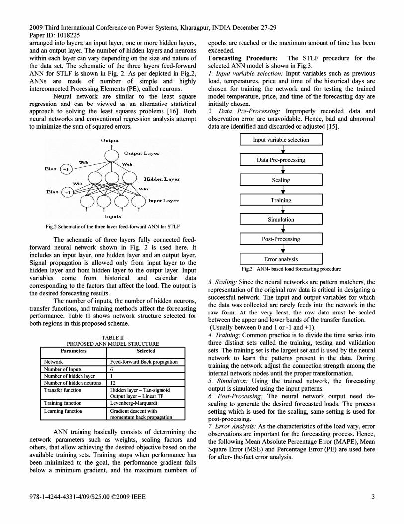
epochs are reached or the maximum amount of time has beenexceeded.Forecasting Procedure: The STLF procedure for theselected ANN model is shown in Fig.3.1. Input variable selection: Input variables such as previousload, temperatures, price and time of the historical days arechosen for training the network and for testing the trainedmodel temperature, price, and time of the forecasting day areinitially chosen.2. Data Pre-Processing: Improperly recorded data andobservation error are unavoidable. Hence, bad and abnormaldata are identified and discarded or adjusted [15].

2009 Third International Conference on Power Systems, Kharagpur, INDIA December 27-29Paper ID: 1018225arranged into layers; an input layer, one or more hidden layers,and an output layer. The number of hidden layers and neuronswithin each layer can vary depending on the size and nature ofthe data set. The schematic of the three layers feed-forwardANN for STLF is shown in Fig. 2. As per depicted in Fig.2,ANNs are made of number of simple and highlyinterconnected Processing Elements (PE), called neurons .

Neural network are similar to the least squareregression and can be viewed as an alternative statisticalapproach to solving the least squares problems [16]. Bothneural networks and conventional regression analysis attemptto minimize the sum of squared errors.

O u rp'ur Input variable selection

Bias

Bia s

O 'urpuf L a y .. r

'Hfdd .. n L ay.. r

lll},"t L a y .. r

Data Pre-processing

Scaling

Training

1l\IJuts

Fig.2 Schematic ofthe three layer feed-forward ANN for STLF

The schematic of three layers fully connected feed­forward neural network shown in Fig. 2 is used here. Itincludes an input layer, one hidden layer and an output layer.Signal propagation is allowed only from input layer to thehidden layer and from hidden layer to the output layer. Inputvariables come from historical and calendar datacorresponding to the factors that affect the load. The output isthe desired forecasting results .

The number of inputs, the number of hidden neurons,transfer functions , and training methods affect the forecastingperformance. Table II shows network structure selected forboth regions in this proposed scheme.

TABLE IIPROPOSED ANN MODEL STRUCTURE

Parameters Selected

Network Feed-forward Back propagat ion

Number oflnouts 6Number of hidden laver INumber of hidden neurons 12Transfer function Hidden layer - Tan-sigmoid

Output layer - Linear TFTraining function Levenberg-Marquardt

Learning function Gradient descent withmomentum back oronaaation

ANN training basically consists of determining thenetwork parameters such as weights , scaling factors andothers, that allow achieving the desired objective based on theavailable training sets. Training stops when performance hasbeen minimized to the goal, the performance gradient fallsbelow a minimum gradient, and the maximum numbers of

978-1-4244-4331-4/09/$25.00 ©2009 IEEE

Simulation

Post-Processing

Error analvsis

Fig.3 ANN- based load forecasting procedure

3. Scaling: Since the neural networks are pattern matchers, therepresentation of the original raw data is critical in designing asuccessful network. The input and output variables for whichthe data was collected are rarely feeds into the network in theraw form. At the very least, the raw data must be scaledbetween the upper and lower bands of the transfer function.(Usually between 0 and 1 or -1 and +1).4. Training: Common practice is to divide the time series intothree distinct sets called the training, testing and validationsets. The training set is the largest set and is used by the neuralnetwork to learn the patterns present in the data. Duringtraining the network adjust the connection strength among theinternal network nodes until the proper transformation.5. Simulation: Using the trained network, the forecastingoutput is simulated using the input patterns .6. Post-Processing: The neural network output need de­scaling to generate the desired forecasted loads. The processsetting which is used for the scaling, same setting is used forpost-processing.7. Error Analysis: As the characteristics of the load vary, errorobservations are important for the forecasting process. Hence,the following Mean Absolute Percentage Error (MAPE) , MeanSquare Error (MSE) and Percentage Error (PE) are used herefor after- the-fact error analysis .

3

which are very much better than the R square value ofmultiple regression models Le.71% oflITR and 88% ofNSW.Also MAPE and MSE values of ANN models are very low ascompared to multiple regression models. Fig.5 shows that howwell the predicted data and actual data points are close to eachother compared to Fig.4. The results depicted in Fig. 6 and 7,are of the IITR campus and Fig. 8 to 11 are of the Australia'sNSW state.

(I)

(40)

YF i is the forecasted load.

2009 Third International Conference on Power Systems, Kharagpur, INDIA December 27-29Paper ID: 1018225

:fMAP'. .!. ~ IO'dt - l'flJl Ite lOP

N 61 1At

:I NMIl. - ~O'~ - l'Ft)'N1i:Where YA I is the actual load and

1.5

)( 1 0 '"

oo

00

1T a rg et s T

1Targ et s T

O u t p u t s v s . Ta r get s . R=O.9 4245

O u -p u t s v s , Target s . R=O _9 9 3 8 8

o D a t a P c tn t s1 .4 --B e s t Line ar F it

········· A = T

° t,'=5- - - - - - - -7"-- - - - - - ----:-'

X 104

15rr:===== = === ==;-- - - - - - - -,

o Dat a P o int s1 .4 --Best Lin e ar F it

. -A = T

°t,'=5-------~-------~

x 1 04

1 . 5 Fr===:====::::::===i,------'~------,

0 .9

0 .7

« 1 .1

~.e- 1<5

1 .2

Fig.4 Correlation of actual (T) and predicted (A) load by MR for the NSWstate

....---...."...--::------,::---."....

0 .8

0 .6

0 .6

0 .7

0 8

0 .9

« 1 . 1

~-s 1C)

Fig .5 Correlation of actual (T) and predicted (A) load by ANN for NSW state.

1 .2

Fig. 6 shows the results of actual and forecasted a dayahead load of the 1sl week of Oct.08 for the IITR campus, Fig.8 and 10 shows the results of actual and forecasted half hourahead load for the 2 Jan.2009 and 6 Jan.2009 ofNSW state byMR and ANN respectively . It is clear from the results thatforecasted load patterns are very much similar to the actualone by ANN method. The % errors on load forecasting byMR and ANN for the respective week and days are shown inFig. 7 oflITR and Fig. 9 and 110fNSW state. By ANN the %errors are less than multiple regressions .

Fig.12 and 13 shows the results of half hour wiseMAPE and MSE of Friday, 2 Jan.09 day for the NSW state.Table V shows the day wise MAPE and MSE of l SI week ofOct.08 for the IITR campus.

Table VI to IX shows the average comparativeperformance results of the proposed methods for the IITRcampus and the Australia's NSW state respectively . Themaximum values of MAPE are 5.41% of IITR and 1.95% ofNSW for the case of ANN whereas it is 7.68% of IITR and

Parameters ByMR By ANN

R value 0.8484 0.9213R Souare 0.7198 0.8499MSE 2.2876 1.3183MAPE 6.4031 4.5444

Parameters By MR By ANNR value 0.9424 0.9938

R Square 0.8882 0.9879

MSE 0.2139 0.0233MAPE 4.02 1.31

From Table III and IV, we analyze that the R squarevalue of ANN models are 84% for IITR and 98% for NSW,

TABLE IVPERFORMANCE OF MR ANDANN MODELSFOR THE NSW STATE

V. TEST RESULTS

In this paper, two separate regions data are used fortesting: these are lIT Roorkee campus and Australia's NSWstate. For both regions year 2008 historical data are used forregressing and training the models: multiple regression andneural network. The performance of the developed classicalregression model and ANN model for load profile forecastingwas tested using July 08 and October 08 months for IITRcampus and January 09 month for NSW state, that were notincluded in the training and regression sets. The forecastedhalf hourly load and a day ahead load for the several dayswere estimated. But here only two days half hourly load ofJan.09 month for NSW region and next seven days load ofOct.08 month for IITR campus region are presented. Theperformance of classical multiple regression and ANN modelsare measured by MAPE, MSE and PE. In addition with theseparameters , the fitness of actual and predicted load is tested byRand R square values. R is a measure of the correlationbetween the observed (Actual) value and the predicted valueof the criterion variable i.e. load. R square is the coefficient ofdetermination which is the square of correlation R. It measuresthe goodness of fit of the fitted regression line to a set of data.The values of these R and R square should be 1 for bestmodel. In essence, this is a measure of how good a predictionof the criterion (dependent) variable we can make by knowingthe predictor (independent) variables. Table III and IV showthe performance of the multiple regression and ANN modelsfor the IITR campus and NSW state. Fig. 5 and 6 shows thecorrelation of actual load and predicted load for the NSWstate.

TABLE IIIPERFORMANCE OF MR ANDANN MODELSFOR THE IITR CAMPUS

978-1-4244-4331-4/09/$25.00 ©2009 IEEE 4

50

50

45

45

40

40

6 Jan. 2009 Tuesday

_._._.- 1 .MR

--2 .F F BP NN

Ic=J 1 M R I_ 2 .F F BP NN

7.68 5.41 2.63 1.474.84 2.58 0.79 0.22

15 20 25 3 0 3 5T im e H a lf hourl y -4 8 po in t s

By MR By ANN By MR By ANN

105

, . . , .______ • .. • L. •

, . . ., . . .: : : :

I-Oct-08 1.18 1.18 0.07 0.482-0ct-08 1.62 0.19 0.09 0.003-0ct-08 3.24 1.77 0.32 0.094-0ct-08 10.49 4.11 2.16 0.335-0ct-08 4.62 2.21 0.42 0.106-0ct-08 10.31 1.14 1.87 0.467-Oct-08 4.64 2.04 0.65 0.13

TABLE VDAY WISE MAPE AND MSE FOR THE IITR CAMPUS

I MAPE% I MSE

TABLE VIAVERAGE MAPE AND MSE FOR THE IITR CAMPUS

I MAPE% I MSEBy MR ByANN By MR By ANN

4th week ofJUL.08Ist week ofOCT.08

1 21-n-~-~-~-~--~-r=;:~~=::::c:==il

10

1 2 0 0 0

1 10 0 0

13000r - ' - ' - - '-- ' - ' - - '-- :;== = =:=:==:====j1

3 9 0 0 0

§ 10000

-4

-6

-8

-10

-12 0L---"-..L5-----,-l LO----'15,------,2LO----'25=-----,3"'0----'35L--.L..--,L-----'

Tim e Half hourl y-48 po int s

Fig.ll % Error in forecasted load by MR and ANN offor the NSW state

Fig.9 % Error in forecasted load by MR and ANN of2 Jan. 2009, Friday forthe NSW state

Fig.1O Forecasted output compared with actual load by MR and ANN of6 Jan. 2009 Tuesday for the NSW state

8 1 -----;- ----,- ;-- ;-- ,------,-- ---;;:= = ==0==11

TUE

4540

_ ._ ._ . - l.MR

--2 .F F B P N N

10

I , , , , , I ,. ~ ----,----_ ----.. ----_. ~ ---.. ------ --~ ------I , , , , , I II , , , , , I II , , , , , I II , , , , I I I

THU FR I SAT S UN MOND ays of Week 1at O et.OB to 7 t h O ct .OB

5

15,-;-- --;- --,- ---,- - ,-- ;-- :;:= = = =::'====]J

600 0

550011l0----'L---'------'---'---:.:----'L---'------'---'---5~

850 0

800 0

-5

10

-10

~ 7500

580

560

540

~ 52 0

.3 500

480

460

44 0

420W E D THU MON TUE

~w 0

""

Fig. 6 Forecasted Output compared with actual load by MR and ANN of Istweek ofOct.O8 for the IlTR campus

15 , - - - , - - - , - - - , - - -----,c-r== = = =::== =]J ~

w

""

2009 Third International Conference on Power Systems, Kharagpur, INDIA December 27-29Paper ID: 10182255.12% of NSW for the case of multiple regressions. Themaximum values ofMSE are 1.47 ofIITR and 0.053 ofNSWfor the case of ANN whereas it is 2.63 of IITR and 0.28 ofNSW for the case of multiple regressions. From Table VIIand IX, it indicates that the ANN model gives less % errorcompared to multiple regressions.

600 [:::;:::e:~-:-':---:---:---:I======'il

15 20 25 30 35Time Half hourly-48 points

Fig.8 Forecasted Output compared with actual load by MR and ANN of 2 Jan.2009, Friday for the NSW state

Fig. 7 % Error in forecasted load by MR and ANN of Ist week of Oct.08 forthe IlTR campus

90001,--:-:-:-:-~-:-:r=======j~

5 10 15 20 25 30 35Time H a lf h o u rly - 4 8 p o int s

40 45 50

2

5 10 15 20 25 30 3 5Tim e H a lf h ou rl y-48 poi nt s

40 45 50

978-1-4244-4331-4/09/$25.00 ©2009 IEEE 5

[I] Abdel-Aal RE, AI-Garni AZ. Forecasting monthly electric energyconsumption in Eastern Saudi Arabia using univariate time seriesanalysis. Energy 1997:22(11):1059-69

[2] Saab S Badr E, Nasr G. Univariate and forecasting of energyconsumption case of electricity in Lebanon. Energy 2001;26(1):1-14.

[3] Papalexopoulos , Hesterberg TC. A regression-based approach toshort-term load forecasting IEEE Trans Power Systems1990;5(4):1535-50.

[4] Peng, Hubele NF, Karadi GG. Advancement in the application ofneural networks for short-term load forecasting . IEEE Trans PowerSystems 1992;7(1):250-7.

[5] Park DC, EI-Sharkawi MA, Marks II RJ, Atlas LE, Damborg MJ.Electric load forecasting using an artificial neural network. IEEETrans Power Systems 1991; 6(2):442-9.

[6] Vermaak J, Botha EC. Recurrent neural networks for short-term loadforecasting. IEEE Trans Power Systems 1998; 13(1):126-32.

[7] Chow TWS, Leung CT. Neural network based short-term loadforecasting using weather compensation. IEEE Trans Power Systems1996;1l(4):1736-42.

[8] Rahman S, Hazim O. A generalized knowledge-based short-term loadforecasting technique. IEEE Trans Power Systems 1993;8(2):508-14.

[9] Gao R, Tsoulakas LH. Neural-wavelet methodology for loadforecasting . J Intel Robot Systems 2001; 31:149-57.

[10] Tzafestas S, Tzafestas E. Computational intelligence techniques forshort-term electric load forecasting . J Intel Robot Systems 2001;31:7-68.

[II] Jia NX, Yokoyama R, Zhou YC, Gao ZY. A flexible long-term loadforecasting approach based on new dynamic simulation theory ­GSIM. Electr Power Energy Systems 2001;23:549-56.

[I 2] Padmakumari K, Mohandas KP, Thiruvengadam S. Long termdistribution demand forecasting using neuro fuzzy computations .Electr Power Energy Systems 1999;21:315-22

[I3] F. C. Schwapper , W. C. Caramanis , R. D. Tabors, and R. E. Bohn,Spot Pricing ofElectricity, Kluwer Academic Publisher 1988.

[I4] Damodar N. Gujarati, Sangeetha , Basic Econometrics Book.[I5] H. Chen, "An Implementation of Power System Short-Term Load

Forecasting ," Power System Automation, China, Dec 1997.[I 6] H.White, A.R.gallant , K.Hornik, MStinchobe and J.Woodridge,

Artificial Neural Networks Applications and Learning Theory ,Blackwell , Cambridge, MA, 1992.

[I 7] NEMMCO web site www.nemmco.com

Barjeev Tyagi (b'1964) received B. Tech. degree in Electrical Engineeringfrom University of Roorkee (India) in 1987 and Ph. D. degree from lITKanpur in 2006. Presently, he is a faculty member in Electrical EngineeringDepartment at Indian Institute of Technology, Roorkee (India). His research

REFERENCES

Mohan Akole (b'1973) received B.E. degree in Instrumentation Engineeringfrom S.G.G.S. COE & T, Nanded in 1997 and M. Tech in SystemEngineering and Operation Research at lIT Roorkee (India) in 2009.Presently , he is a faculty member in Instrumentation Engineering Departmentat Government College of Engineering, Chandrapur (India). His researchinterests include artificial intelligence system, power system deregulation ,instrumentation and control system.

actual load. The performance evaluation parameters MAPE,MSE and percentage error have used for testing this proposedforecasting models. The values of these parameters are verylow for ANN model as compared to the regression model.Also statistical parameters such as R and R square have beenused here for checking the goodness of models and thesevalues of ANN model have much better than the regressionmodel. It is clear from the testing results that the ArtificialNeural network technique works more effectively compared tothe conventional Multiple Regression technique .

Maximum

12.82 12.127.86 4.10

ByMR ByANNByMR ByANNMinimum

5

I-Jan-09 4.1558 1.9220 0.1290 0.03312-Jan-09 3.7575 1.2372 O.1116 0.01343-Jan-09 3.2345 1.2532 0.0919 0.01304-Jan-09 3.6199 1.0168 0.0987 0.01325-Jan-09 5.0001 1.7619 0.2533 0.03726-Jan-09 5.1282 1.9561 0.2809 0.04857-Jan-09 4.8493 1.9324 0.2772 0.0538

% ErrorMinimum Maximum

ByMR By ANN ByMR By ANN

I-Jan-09 -12.2969 -7.9034 5.7260 2.87952-Jan-09 -11.8621 -2.7238 6.9905 3.20013-Jan-09 -11.7621 -4.1113 7.6775 4.03834-Jan-09 -9.0273 -5.2572 8.7933 4.51365-Jan-09 -8.9123 -4.5238 10.7668 3.75536-Jan-09 -10.6337 -4.2671 10.4173 3.68757-Jan-09 -10.2058 -6.3196 9.6701 4.7630

4th week of JUL.08 -18.75 -2.651st week of OCT.08 -10.49 -3.90

0.7

0.6

en 0.5Cl

:ii-, 0.4-g'"'0 0.3wfJ)

::;: 0.2

0.1

15 20 25 30 35Time Half hourly-48 points

Fig.13 Half hour wise MSE result of Friday, 2 Jan.09 day for the NSW state

TABLE IXCOMPARISON OF RESULTS BY % ERRORFOR THE NSW STATE

2009 Third International Conference on Power Systems, Kharagpur, INDIA December 27-29Paper ID: 1018225Fig.12 Half hour wise MAPE result of Friday, 2 Jan.09 day for the NSWstate

TABLE VlllAVERAGE MAPE AND MSE FOR THE NSW STATE

IMAPE (%) I MSE

---- By MR By ANN By MR By ANN

TABLE VIICOMPARISON OF RESULTS BY % ERRORFOR THE IITR CAMPUS

% Error

VI. CONCLUSION

An ANN based short term load forecasting methodthat uses feed-forward neural network and a back-propagationtraining method is proposed in this paper, electricity price hasbeen considered as one of the factors affecting the load inderegulated markets. Load forecasting plays a very importantrole in the restructured power system. The IITR campus dataand publicly available data of Australia 's NSW state wereused in this paper for testing and demonstrating theperformance of the multiple regression and artificial neuralnetwork models for the short term load forecasting (STLF).From the results as discussed above, it is observed that theforecasted load by ANN model is very much similar to the

978-1-4244-4331-4/09/$25.00 ©2009 IEEE 6

2009 Third International Conference on Power Systems, Kharagpur, INDIA December 27-29Paper ID: 1018225interests include control system, power system deregulation, power systemoptimization and control.

978-1-4244-4331-4/09/$25.00 ©2009 IEEE 7