AUTOMATIC LOAD FREQUENCY CONTROL

Cairo University – Faculty of EngineeringEnergy Research CenterDiploma in Control System Project

AUTOMATIC LOAD FREQUENCY CONTROL

Presented to:

Prof. Dr. M. M . EL-METWALLYProject group:

Eng. Mahmoud saad eldinEng. Hany ali husseineng. Osama othman

Load frequency control 1

eng.mohammed shabkaeng.randaeng.shimaaeng.ibrahim


Chapter 1: INTRODUCTION

Chapter 2:

2.Load frequency control of single area system

2.1Dynamics of the power generating system

2.1.1SPEED GOVERNOR

2.1.2HYDRAULIC VALVE ACTUATOR

2.1.3TURBINE – GENERATOR

2.1.4 STATIC PERFORMANCE OF SPEED GOVERNOR

2.1.5Closing the ALFC loop

2.1.6Static Response of primary ALFC loop

2.1.7Dynamic Response of ALFC loop

2.1.8PROPORTIONAL PLUS INTEGRAL CONTROL Load frequency control 3

2.2Application (Matlab & Result )

2.3discussion

Chapter 3:3.Load frequency control of Two area system

3.1 Modeling of Tow area system3.1.1 Static Response of primary ALFC

loop

3.1.2 Dynamic Response of ALFC loop

3.1.3 Tie line Bias control for two

area

3.2 Application (Matlab & Result )

3.3 Discussion

Chapter 4: Optimal load frequency control 4.1 : Optimal of single area4.2 : Optimal of two area4.3 : Application of optimal control

Chapter 5: Comparison between conventional and optimal load frequency control

Chapter 6: Conclusion References :


INTRODUCTION:

The main objective of power system operation and controlis to maintain continuous supply of power with an acceptable quality, to all the consumers in the system. The system will be in equilibrium, when there is a balance between the power demand and the power generated. As the power in AC form has real and reactivecomponents: the real power balance; as well as the reactive power balance is to be achieved.

Thus steam input to turbine must be continuously regulated to match the active power demand. The system frequency otherwise will change which is not desirable. (A change in the electric power consumption will result in a deviation of the frequency from its steady state value. The consumers require a value of frequency and voltage constant. To maintain these parameters, controlsare required on the system and must guarantee a good level of voltage with an industrial frequency).

Excitation of the generator must also be maintained continuously to match the reactive power demand; otherwise the voltage at various system buses may go beyond the specified limit. Manual regulation is not possible. There are two basic control mechanisms used to


Chapter 1

achieve reactive power balance (acceptable voltage profile) and real power balance (acceptable frequency values). The former is called the automatic voltage regulator (AVR) and the latter is called the automatic load frequency control (ALFC) or automatic generation control (AGC). Thus, Voltage is maintained by the control of excitation of the generator and frequency is maintained by the elimination of the difference in powerbetween the power provided by the turbine and the power required by the load. It is known that although the loads are time-variant, the variations are relatively slow. The controllers are set for a particular operatingcondition and they take care of small change in load demand without frequency and voltage exceeding the précised limits .As the change in load demand becomes large, the controllers must be reset either manually or automatically.

Load frequency control

The main purpose of operating the load frequencycontrol is to keep uniform the frequency changesduring the load changes. During the power systemoperation rotor angle, frequency and active power arethe main parameters to change. In multi area system a change of power in one areais met by the increase in generation in all areasassociated with a change in the tie-line power and areduction in frequency. In the normal operating state


the power system demands of areas are satisfied atthe nominal frequency.

The basic role of ALFC is:

1.To maintain the desired megawatt output powerof a generator matching with the changing load

2. To assist in controlling the frequency oflarger interconnection.

3. To keep the net interchange power between poolmembers, at the predetermined values.


Load frequency control of single area system

2.1 Dynamics of the power generating system

The real power control mechanism of a generator is shown in Fig. 1. The main parts are: 1) Speed changer 2) Speed governor 3) Hydraulic amplifier 4) Control valve. They areconnected by linkage mechanism. Their incremental movements are in vertical direction. In reality these movements are measured in millimeters; but in our analysiswe shall rather express them as power increments expressedin MW or p.u. MW as the case may be. The movements are assumed positive in the directions of arrows. Corresponding to “raise” command, linkage movements will be: “A” moves downwards; “C” moves upwards; “D” moves upwards; “E” moves downwards. This allows more steam or water flow into the turbine resulting incremental increasein generator output power. When the speed drops, linkage point “B” moves upwards and again generator output power will increase.


Chapter 2

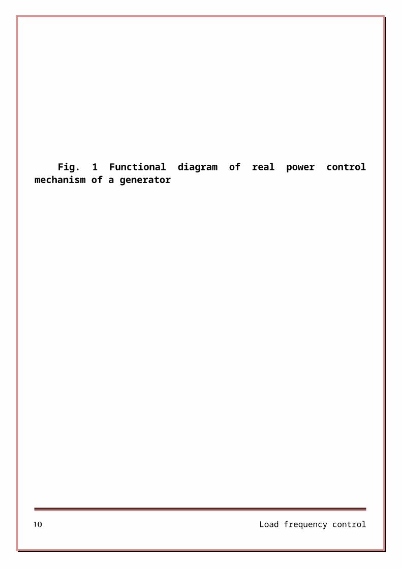
Fig. 1 Functional diagram of real power controlmechanism of a generator


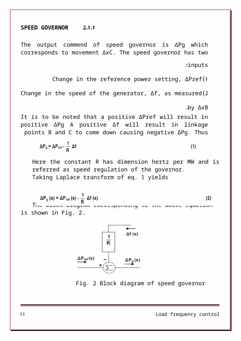
2.1.1SPEED GOVERNOR

The output commend of speed governor is ΔPg whichcorresponds to movement ΔxC. The speed governor has two

inputs :1 )Change in the reference power setting, ΔPref 2 )Change in the speed of the generator, Δf, as measured

by ΔxB.It is to be noted that a positive ΔPref will result inpositive ΔPg A positive Δf will result in linkagepoints B and C to come down causing negative ΔPg. Thus

Here the constant R has dimension hertz per MW and isreferred as speed regulation of the governor.Taking Laplace transform of eq. 1 yields

The block diagram corresponding to the above equation is shown in Fig. 2.

Fig. 2 Block diagram of speed governor


2.1.2HYDRAULIC VALVE ACTUATOR

The output of the hydraulic actuator is ΔPv. This depends on the position of main piston, which in turn depends on the quantity of oil flow in the piston. For a small change ΔxD in the pilot valve position, we have

The constant “kH” depends on the orifice, cylindergeometries and fluid pressure.

The input to ΔxD are ΔPg and ΔPv. It is to be notedthat for a positive ΔPg, the change ΔxD is positive.Further, for a positive ΔPv, more fuel is admitted,speed increases, linkage point B moves downwardscausing linkage points C and D to move downwardsresulting the change ΔxD as negative. Thus


Laplace transformation of the last two equations are:

Eliminating ΔxD and writing ΔPv (s) in terms of ΔPg (s), we get

where TH is the hydraulic time constant given by

In terms of the hydraulic valve actuator’s transfer function GH (s), eq. 5 can be written as

Hydraulic time constant TH typically assumes values around 0.1 sec. The block diagram of the speed governortogether with the hydraulic valve actuator is shown in

Fig. 3.


Fig. 3 Block diagram of speed governor together with hydraulic valve actuator

2.1.3TURBINE – GENERATOR In normal steady state, the turbine power PT keepsbalance with the electromechanical air-gap power PGresulting in zero acceleration and a constant speed and

frequency.During transient state, let the change in turbine powerbe ΔPT and the corresponding change in generator power

be ΔPG. The accelerating power in turbine generator unit = ΔPT – ΔPG


Thus accelerating power = ΔPT (s) - ΔPG (s)

)8)If ΔPT - ΔPG is negative, it will decelerate.The turbine power increment ΔPT depends entirely upon the valve power increment ΔPv and the characteristic ofthe turbine. Different type of turbines will have different characteristics. Taking transfer function with single time constant for the turbine, we can write

The generator power increment ΔPG depends entirely uponthe change ΔPD in the load PD being fed from thegenerator. The generator always adjusts its output soas to meet the demand changes ΔPD. These adjustmentsare essentially instantaneous, certainly in comparison

with the slow changes in PT.We can therefore set

In view of equations 8,9 and 10,

the block diagram developed is updated as shown in Fig.4. This corresponds to the linear model of primary ALFC

loop excluding the power system response.


Fig. 4 Block diagram corresponding to primary loop of

ALFC excluding power system response 2.1.4 .STATIC PERFORMANCE OF SPEED GOVERNOR

The present control loop shown in Fig. 4 is open. Wecan nevertheless obtain some interesting informationabout the static performance of the speed governor. Therelationship between the static signals (subscript “0”)

is obtained by letting we obtain directly from Fig. 4

Note that at steady state, ΔPT is equal to ΔPG. i.e. ΔPT 0 = ΔPG 0

We consider the following three cases.Case A The generator is synchronized to a network of verylarge size, so large in fact, that its frequency willbe essentially independent of any changes in the poweroutput of this individual generator (“infinite”

network). Since Δf0 = 0, the above eq. becomes Load frequency control 16

Thus for a generator operating at constant speed,(or frequency) there exists a direct proportionality

between turbine power and reference power setting .Thus for a generator operating at constant speed, (or frequency) there exists a direct proportionality

between turbine power and reference power setting.ΔPT 0 = ΔPref 0 i.e. when the generator is operating atconstant frequency, if the speed changer setting is INCREASED,(DECREASED) turbine output power will

increase ( decrease ) to that extent.


Case B

Now we consider the network as “finite”. i.e. itsfrequency is variable. We do, however, keep the speedchanger at constant setting. i.e. ΔPref = 0. From eq.

(11)

The above eq. shows that for a constant speed changersetting, the static increase in turbine power output is

directly proportional to the static frequency drop.

The above eq. (13) can be rewritten as Δf 0 = - R ΔPT0. This means that the plot of f 0 with respect to PT 0

(or PG 0) will be a straight line with slope of – R.We remember that the unit for R is hertz per MW. Inpractice, both the frequency and the power can be

expressed in per unit.Case C

In general case, changes may occur in both the speed changer setting and frequency in which case the

relationship


For a given speed changer setting, ΔPref 0 = 0 andhence Δf0 = - R ΔPT 0. In a frequency-generation power

graph, this represents a straight line with a slope= - R.

For a given frequency, Δf 0 = 0 and hence ΔPT 0 =ΔPref 0. This means that for a given frequency,generation power can be increased or decreased by

suitable raise or lower command . Thus the relationship

represents a family of sloping lines as depicted in Fig. 5, each line corresponding to a specific speed

changer setting.

Fig. 5 Static frequency-power response of speed governor (R = 0.04 p.u.)The thick line shows that corresponding to 100% ratedfrequency, the output power is 100 % of rated output. Butfor the new speed changer setting as shown by the dottedline, for the same 100% rated frequency, output power is50 % of rated output. Hence the power output of the


generator at a given frequency can be adjusted at will, bysuitable speed changer setting. Such adjustment will beextreme importance for implementing the load division as

decided by the optimal policy.

2.1.5 .CLOSING THE ALFC LOOP

We observed earlier that the loop in Fig. 4 is “open”. Wenow proceed now to “close” it by finding a mathematicallink between ΔPT and Δf. As our generator is supplyingpower to a conglomeration of loads in its service area, itis necessary in our following analysis to make reasonable

assumptions about the “lumped” area behavior.We make these assumptions:

1.The system is originally running in its normal statewith complete power balance, that is, PG0 = PD0 +losses. The frequency is at normal value f 0. Allrotating equipment represents a total kinetic energy

of W0kin MW sec.

2. By connecting additional load, load demand increasesby ΔPD which we shall refer to as “new” load. (If loaddemand is decreased new load is negative). The


generation immediately increases by ΔPG to match the

new load, that is ΔPG = ΔPD.

3.It will take some time for the control valve in thespeed governing system to act and increase the turbinepower. Until the next steady state is reached, theincrease in turbine power will not be equal to ΔPG.Thus there will be power imbalance in the area thatequals ΔPT - ΔPG i.e. ΔPT – ΔPD. As a result, thespeed and frequency change. This change will beassumed uniform throughout the area. The above saidpower imbalance gets absorbed in two ways. 1) By thechange in the total kinetic K.E. 2) By the change in

the load, due to change in frequency.Since the K.E. is proportional to the square of the speed, the area K.E. is

The “old” load is a function of voltage magnitude andfrequency. Frequency dependency of load can be written

as


The ΔP’s are now measured in per unit (on base Pr) and D

in pu MW per Hz.Typical H values lie in the range 2 – 8 sec.

Laplace transformation of the above equation yields


Equation (22) represents the missing link in the controlloop of Fig. 4. By adding this, block diagram of the

primary ALFC loop is obtained as shown in Fig. 6.

Fig. 6 Block diagram corresponding to primary loopof ALFC

2.1.6Static Response of primary ALFC loop

The primary ALFC loop in Fig. 6 has two inputs ΔPref and ΔPD and one output Δf.


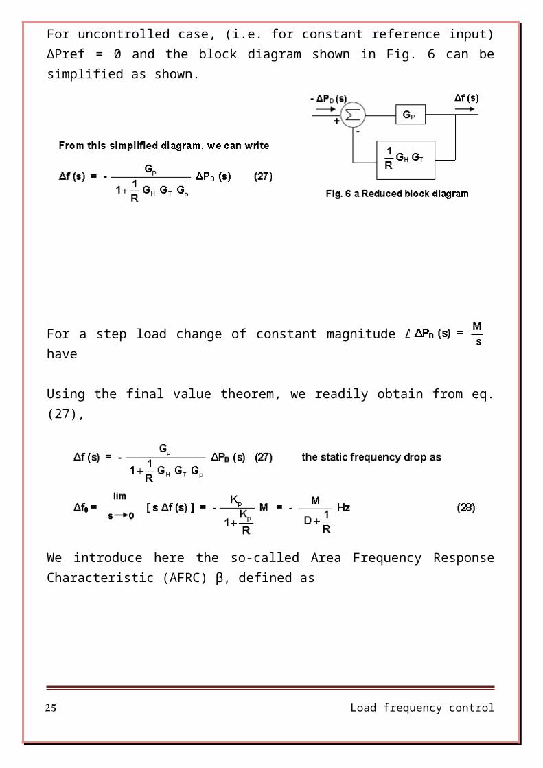
For uncontrolled case, (i.e. for constant reference input)ΔPref = 0 and the block diagram shown in Fig. 6 can besimplified as shown.

For a step load change of constant magnitude ΔPD = M, wehave

Using the final value theorem, we readily obtain from eq.(27),

We introduce here the so-called Area Frequency ResponseCharacteristic (AFRC) β, defined as


2.1.7DYNAMIC RESPONSE OF PRIMARY ALFC LOOP - UNCONTROLLEDCASE We know that

Finding the dynamic response, for a step load, is quitestraight forward. Eq. (27) upon inverse Laplacetransformation yields an expression for Δf (t). However,as GH, GT and Gp contain at least one time constant each,the denominator will be a third order polynomial resultingin unwieldy algebra.

We can simply the analysis considerably by making thereasonable assumption that the action of speed governorplus the turbine generator is “instantaneous” comparedwith the rest of the power system. The latter, asdemonstrated in Example 5 has a time constant of 20 sec,and since the other two time constants are of the order of1 sec, we will perform an approximate analysis by settingTH = TT = 0.


Making use of previous numerical values: M = 0.01 p.u. MW;R = 2.0 Hz / p.u. MW; Kp = 100 Hz / p.u. MW; Tp = 20 sec.

The approximate time response is purely exponential and isgiven by


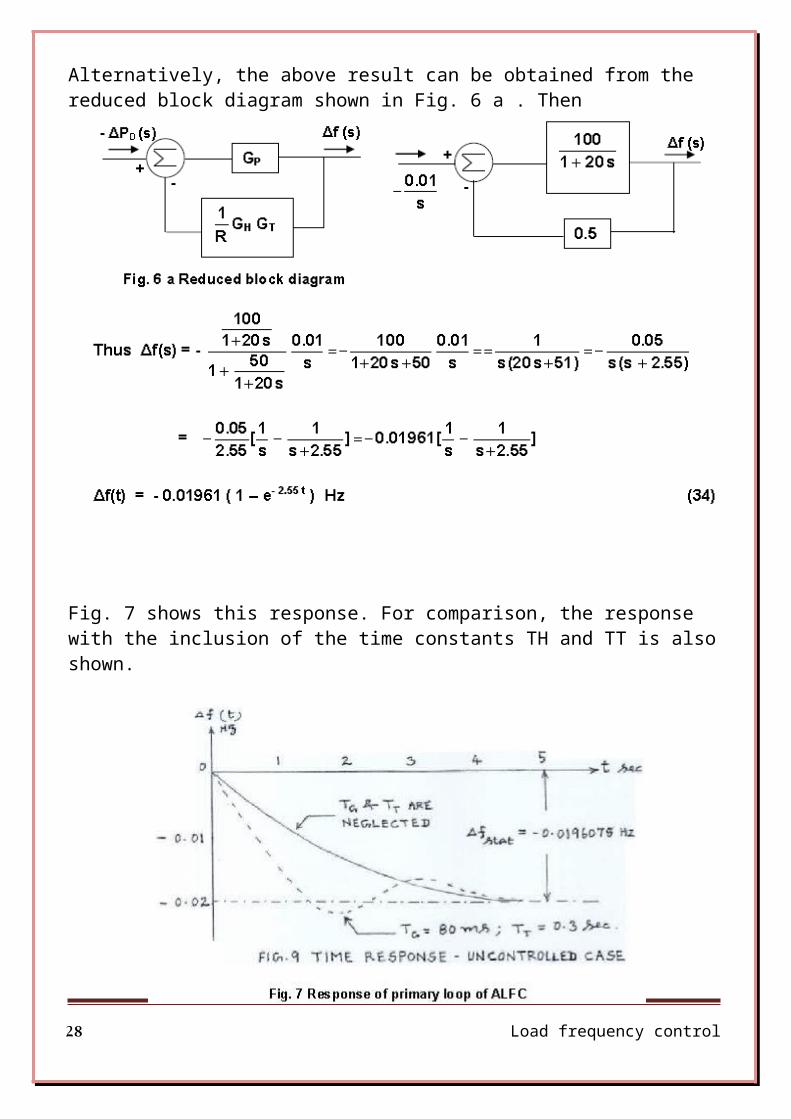
Alternatively, the above result can be obtained from the reduced block diagram shown in Fig. 6 a . Then

Fig. 7 shows this response. For comparison, the response with the inclusion of the time constants TH and TT is alsoshown.


It is to be observed that the primary loop of ALFC does not give the desired objective of maintaining the frequency constant. We need to do something more to bring the frequency error to zero. Before discussing the necessary control which can make the frequency error to zero, we shall shed some light on to the physical mechanism in the primary loop of ALFC.2.1.8 PROPORTIONAL PLUS INTEGRAL CONTROL ( Secondary ALFC

loop)

It is seen from the previous discussion that with the speed governing system installed in each area, for a givenspeed changer setting, there is considerable frequency drop for increased system load.

In the example seen, the frequency drop is 0.01961 Hz for 20 MW. Then the steady state drop in frequency from no load to full load ( 2000 MW ) will be 1.961 Hz.

System frequency specification is rather stringent and therefore, so much change in frequency cannot be tolerated. In fact, it is expected that the steady state frequency change must be zero. In order to maintain the frequency at the scheduled value, the speed changer setting must be adjusted automatically by monitoring the frequency changes.

For this purpose, INTEGRAL CONTROLLER is included. In theintegral controller the frequency error is first amplifiedand then integrated. Further, a negative polarity is alsoincluded so that a NEGATIVE frequency deviation will giverise to RAISE command. The signal fed into the integratoris referred as Area Controlled Error (ACE). For this caseACE =ΔF. Thus


Taking Laplace transformation

The gain constant KI controls the rate of integration andthus the speed of response of the loop.

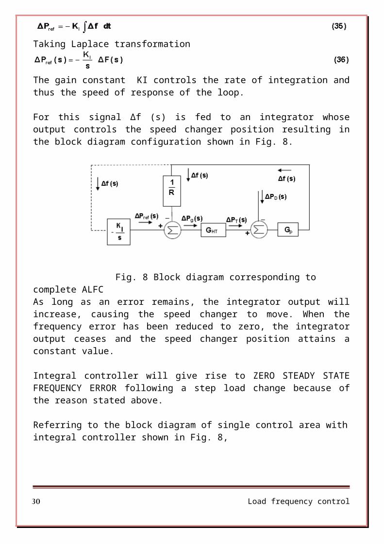
For this signal Δf (s) is fed to an integrator whoseoutput controls the speed changer position resulting inthe block diagram configuration shown in Fig. 8.

Fig. 8 Block diagram corresponding to complete ALFCAs long as an error remains, the integrator output willincrease, causing the speed changer to move. When thefrequency error has been reduced to zero, the integratoroutput ceases and the speed changer position attains aconstant value.

Integral controller will give rise to ZERO STEADY STATEFREQUENCY ERROR following a step load change because ofthe reason stated above.

Referring to the block diagram of single control area withintegral controller shown in Fig. 8,


IN STATIC FREQUENCY DROP FOLLOWING A STEP LOAD CHANGE

Thus static frequency drop due to step load change becomeszero, which is a desired feature we were looking. This is made possible because of the integral controller that has been introduced.

IN DYNAMIC ANALYSIS

Let us assume time constants TH and TT as zero


Then GH T = 1. For a step load change of ΔPD = M, from eq.(37) we get

Multiplying the numerator and denominator by s R( 1 + s Tp) we get

Dividing the numerator and denominator by R Tp the above equation becomes

We obtain the time response Δf (t)upon Laplace inverse transformation of this expression in the right hand side of above equation. Since response depends upon the poles of the denominator polynomial, let us examine it.

A second order system of type as2 + bs + c = 0 will be stable if the coefficients a, b and c are greater than


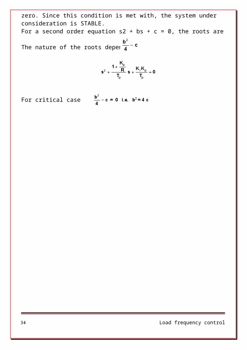
zero. Since this condition is met with, the system under consideration is STABLE.For a second order equation s2 + bs + c = 0, the roots are

The nature of the roots depends on

For critical case


Now, both the roots are real, equal and negative. For thiscritical case

Super critical case

When b2 < 4 c the roots are complex conjugate and the solution is exponentially damped sinusoidal. For this casethe integral gain constant KI is obtained from

When the system is said to be super-critical. Due to damping present, the final solution will tend to zero. However, the solution will be oscillatory type.

Sub-critical case

When b2 > 4 c the roots are real and negative. For this case, the integral gain constant KI is given by

This case is referred as sub-critical integral control. Inthis case the solution contains terms of the typeand it is non-oscillatory. However, finally the solutionwill tend to zero.


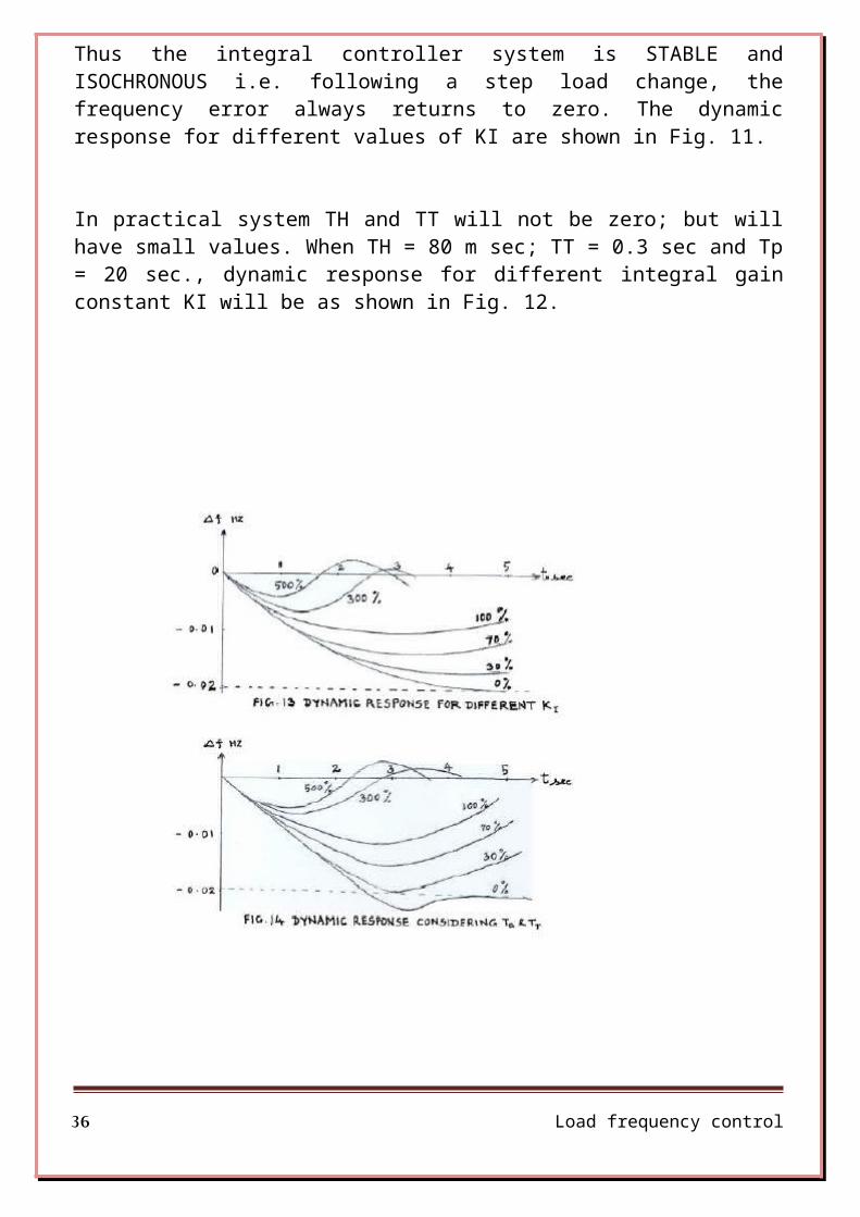
Thus the integral controller system is STABLE andISOCHRONOUS i.e. following a step load change, thefrequency error always returns to zero. The dynamicresponse for different values of KI are shown in Fig. 11.

In practical system TH and TT will not be zero; but willhave small values. When TH = 80 m sec; TT = 0.3 sec and Tp= 20 sec., dynamic response for different integral gainconstant KI will be as shown in Fig. 12.


2.2Application :Matlab simulation For uncontrolled single area by simulinkfig. shown:

Simulink model of single area as shown in the fig. contains of a model of a governer characteristic equation, turbine, load and a kind of disturbance. a case study :Turbine time constant (Tτ)=0.5s,Speed regulator time constant (τg)=0.2s,Generator inertia constant (H)= 5s,Speed regulation rate( R)=0.05


kp12.5s+1

10.5s+1

10.2s+1

1s

y

To W orkspace

-K-

H

FromW orkspace

From the previous fig. it is declared now the affection ofthe load disturbance change where we have changed the disturbance to the system by 20 MW,50MWand 700 MW where the drop in the trend show the affection of the load on the frequency curve in this case the frequency curve goes down proportional with the amount of change in the load applied to the system.

Matlab simulink for a controlled sinle area: in this case we want to check the system stability in case we added an integral term (controlled or compensated term ) to stop on the situation of the change in the frequency at a constant disturbance and changing in the inertia and mass load characteristic gain Kp by (kp=1.25,kp=1.5 ,kp=2)

Case study :


Turbine time constant (Tτ)=0.5s,Speed regulator time constant (τg)=0.2s,Generator inertia constant (H)= 6.25s,Speed regulation rate( R)=0.05


By applied the previous values to the simulink diagram andmake the change in the gain Kp we noticed that frequency behavior affected by the overshoots instantaneously and the goes to stability depending on the values of the gain Kp

2.4 Discussions:

From the previous figures of the uncontrolled ad controlled

simulation of the single area load frequency control its clear

that the effect of the integrator term on the overshot and the


stability of the system by changing in the load disturbance

the integration term reduces the overshoot time and also

the value of the over shoot .

3.Load frequency control of Two area system

3.1 Modeling of Tow area system

SIMULATION OF TWO AREA CONTROL SYSTEM USING SIMULINK:As long as the system frequency is equal to its specified

value (the assumption here),the difference between an area's

actual interchange and its scheduled interchange is known as

the “area control error” (ACE) (the area control error also

includes a term dependent on the deviation in the system

frequency from the specified value; this frequency-dependent

term is not discussed here). The ACE is the single most


Chapter 3

important number associated with control operations; it is

continuously monitored. Anytime the ACE is negative the area

is “under generating” and needs to increase its total

generation. Conversely, if the ACE is positive, the area is

“over generating” and needs to decrease its generation. Over

the last several decades, practically all control areas have

switched to an automatic process known as “automatic

generation control” (AGC). AGC automatically adjusts the

generation in an area to keep the ACE close to zero, which in

turn keeps the net area power interchange at its specified

value. Since the ACE has a small amount of almost random

"ripple" in its value due to the relentlessly changing system

load, the usual goal of AGC is not to keep the ACE exactly at

zero but rather to keep its magnitude close to zero, with an

“average” value of zero. Modern power system network consists

of a number of utilities interconnected together & power is

exchanged between utilities over tie-lines by which they are

connected. Automatic generation control (AGC) plays a very

important role in power system as its main role is to maintain

the system frequency and tie line flow at their scheduled

values during normal period and also when the system is

subjected to small step load perturbations. Many

investigations in the field of automatic generation control of

interconnected power system have been reported over the past

few decades. Literature survey shows that most of the earlier

work in the area of automatic generation control pertains to

interconnected thermal system and relatively lesser attention


has been devoted to automatic generation control (AGC) of

interconnected hydro-thermal systems involving thermal and

hydro subsystems of widely different characteristics]. These

investigations mostly pertain to two equal area thermal

systems or two equal areas hydrothermal systems considering

the system model either in continuous or continuous discrete

mode with step loads perturbation occurring in an individual

area.L

LFC in two- area systemThe AGC of multi-area system can be realized by studying firstthe LFC for atwo-area system

Consider these two areas represented by an equivalent generating unitsinterconnected by a lossless tie line with reactance Xtie . Each area is representedby voltage source behind an equivalent reactance as shown in figure


During normal operation the real power transferred over the tie line is given by:

Equation can be linearized for a small deviation in the flow ∆P12 from thenominal value, that is:

Linear representation of the tie line

Ps: the slope of the power angle curve at the initial operatingangle


Thus

Then


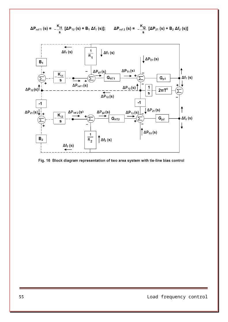
Block diagram representation of two area system with tie-line bias control

3.1.1 Static Response of primary ALFC loop


3.1.2 Dynamic Response of ALFC loop


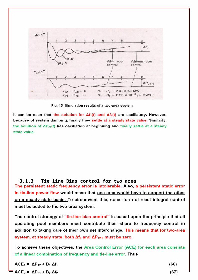
3.1.3 Tie line Bias control for two area


*-Static system response with tie line biascontrol :


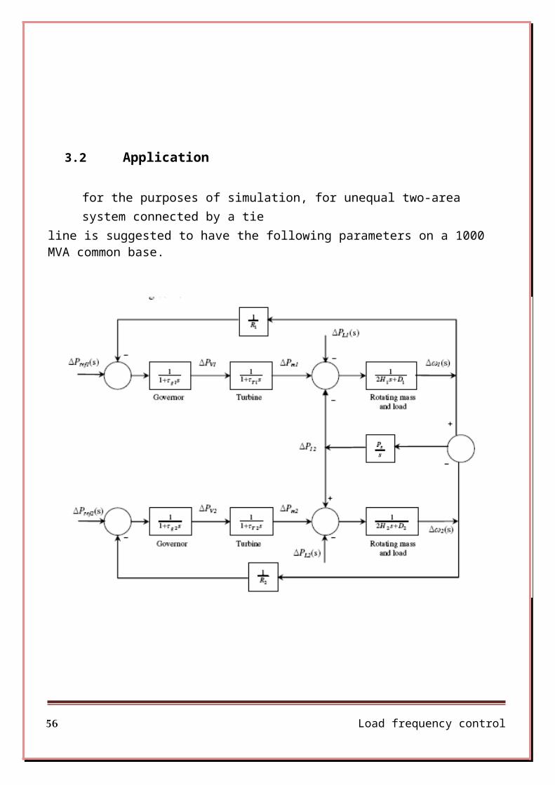
3.2 Application

for the purposes of simulation, for unequal two-area system connected by a tie

line is suggested to have the following parameters on a 1000 MVA common base.


By applying the previous data in the related simulink drawing

below:


10.3s+1

10.6s+1

110s+0.61

0.2s+1

18s+0.9

10.5s+1

1s

Step

-K-

-K-

-K-

Add4

Add3

Add2

Add1

Add

Two area simulation figure

By varying the governor speed regulation for onearea (R) we can notice its affection on the powerdeviation for the two areas and the tie linebetween them the related curve below declare howthe change in the governor speed regulation (R) canmake a power deviation in the tie line between thetwo areas and deviate also the power in the secondarea


Power deviation in two area tie line

Frequency deviation in two area tie line


1s

1s

10.3s+1

10.6s+1

110s+0.61

0.2s+1

18s+0.9

10.5s+1

1s

y1

To W orkspace1

y

To W orkspace

Step

0.3

16.9/16

0.3

20.6/20

1/0.5

1/0.0625

1/0.05

Add6

Add5 Add4

Add3

Add2

Add1

Add

MATLAB Simulation for the Two area system with tie line biased control

Tie line bias control for two areaAdding a biased gain B1=1/R1+D1 that gives theprefer ability for each area to bear its own loadand can share a part of the other load with amountdetermined by the biased gain and that is appearedin the curves below


Results

Power deviation in two area tie line biased control

Frequency deviation in two area tie line biased control


B1=1/R1+D1


4. OPTIMAL CONTROL DESIGN FOR THE LOAD FREQUENCY CONTROL AGAINTST TO LOAD CHANGES

Optimal control is the branch of the modern controltheory. The control design process is realizeddepending on system variables and high performanceoperation of the system in ensured . In the study,optimal control design for the linear systems withquadratic performance (Linear Quadratic Regulator(LQR) is established. The purpose of optimalregulator design is to determine the optimalcontrol rule u*(x,t). For the studied power system,the performance index minimized from the firstentry values to the final state values istransferred. The performance index of the system isselected to obtain the best process between thecost and performance of the control system.Performance index is widely used in optimal controldesign process. It is expressed as quadraticperformance depended on minimum fault and minimumenergy criteria. The system is identified by thestate equation given below.

The problem faced during the system controls is tofind the control rule K(t) vector. The control rulevector below is expressed with the given equation.

The control rule vector minimizes the quadraticperformance index values in the dynamic systemexpression defined in equation . Linear Quadratic


Performance index value (J) is expressed asfollows.

Where, Q is the positive semi-defined matrix and Ris the real symmetric matrix. If the marked minorsof all the elements of Q matrix are not negative, Qmatrix is positive semi-defined matrix. Selectionof Q and R elements are determined according to theweighted relations of state variables and controlentries .

To obtain the above explained solution, we may usethe Lagrange multiplies method. With using ofLagrange multiplies method, limited problem(λ)solution within definite limitations is made.Solution of this function aims to minimize thebelow given limitless function.

To calculate the optimal values, the above givenequation is equalized to zero and its partialderivatives are taken. (*) symbol in the followingexpressions expresses the optimal values.


In optimal solution, when symmetric and positivesemi-defined p(t) matrix that is variable dependingon time is considered, the following expression isgiven.

expression is expressed as equation , it gives theoptimal close cycle rule.

In solution of the above equation, Riccati equationsolution is used. The limit condition for theequation is p(tf)=0. For the time domain solutionof the Diccati equation, [τ,p,K,t,x]=riccatifunction is developed. Riccati equation matrixp(τ), optimal feed-back gaining K(τ), and stateresponse of the system at the beginning x(t) aresolved.Optimal control gaining is the feed-back and timeadjustable state variable. In many practicalapplications, it is sufficient to use the stablestate feed-back gaining. For the systems that donot change with linear time, •p=0. For the solutionof Riccati equation[k,p]=lgr2(A,B,Q,R] function inMatlab Control System Toolbox is used [4] If we usethe LQG control as optimal gaining, by using theLinear Quadratic Regulator(lqry) function, weobtain K feed-back gaining LQR design procedure issimpler and clearer than the traditional controldesign. In traditional controller, the gainingmatrix (K) may be directly selected. The controlexperts prefer Q and R parameters to design theoptimal LQR. Then by using the Riccati


equations, K feed-back gaining matrix is selected .If the system response is not stable, the new Q andR weight matrixes are determined. This is animportant advantage for all the control cycles.

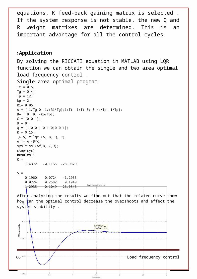
Application: By solving the RICCATI equation in MATLAB using LQR function we can obtain the single and two area optimalload frequency control .Single area optimal program:Tt = 0.5;Tg = 0.4;Tp = 12;kp = 2;R1= 0.05;A = [-1/Tg 0 -1/(R1*Tg);1/Tt -1/Tt 0; 0 kp/Tp -1/Tp];B= [ 0; 0; -kp/Tp];C = [0 0 1];D = 0;Q = [1 0 0 ; 0 1 0;0 0 1];R = 0.15;[K S] = lqr (A, B, Q, R)Af = A -B*K;sys = ss (Af,B, C,D);step(sys)Results :K = 1.4372 -0.1165 -28.9829

S = 0.1960 0.0724 -1.2935 0.0724 0.2582 0.1049 -1.2935 0.1049 26.0846

After analyzing the results we find out that the related curve show how can the optimal control decrease the overshoots and affect the system stability .


Single area optimal program:A = [0.05 6 0 -6 0 0 0; 0 -3.33 3.33 0 0 0 0 ;-5.2083 0 -12.5 0 -0.545 0 0; 0.5450 0 0 -0.05 0 0;0 0 0 6 -0.05 6 0;0 0 0 0 0 -3.33 3.33;0 0 0 0 -5.2083 0 -12.5];B = [0 0;0 0;0 12.5;0 0;0 0;0 0;12.5 0]; BPL=B*PL;C = [0 0 0 0 0 0 1];D = 0;Q = [1 0 0 0 0 0 0;0 1 0 0 0 0 0;0 0 1 0 0 0 0;0 0 0 1 0 0 0;0 0 0 0 1 0 0;0 0 0 0 0 1 0;0 0 0 0 0 0 1];R = [1 0;0 1];[K, P] = lqr2(A, B, Q, R)Af = A - B*Kt=0:0.02:20;[y, x] = step(Af, BPL, C, D, 1, t);Results: K = 0.2587 0.1618 0.0211 1.9479 0.6165 1.2311 0.6296 0.8336 1.4724 0.6685 -0.4770 0.0108 0.0997 0.0211

P = 0.6014 0.5082 0.0667 0.3635 0.0517 0.1087 0.0207 0.5082 0.7364 0.1178 -0.1081 0.0202 0.0642 0.0129 0.0667 0.1178 0.0535 -0.0382 0.0009 0.0080 0.0017 0.3635 -0.1081 -0.0382 5.8492 0.6154 0.8986 0.1558 0.0517 0.0202 0.0009 0.6154 0.4366 0.3839 0.0493 0.1087 0.0642 0.0080 0.8986 0.3839 0.6127 0.0985 0.0207 0.0129 0.0017 0.1558 0.0493 0.0985 0.0504

Af = 0.0500 6.0000 0 -6.0000 0 0 0 0 -3.3300 3.3300 0 0 0 0 -15.6278 -18.4044 -20.8567 5.9624 -0.6803 -1.2462 -0.2640 0.5450 0 0 0 -0.0500 0 0 0 0 0 6.0000 -0.0500 6.0000 0 0 0 0 0 0 -3.3300 3.3300 -3.2343 -2.0228 -0.2640 -24.3485 -12.9141 -15.3893 -20.3697


If we regarded the frequency deviation curvefor the Two area we will find a bigmodification in the behavior of the frequencyafter applying the optimal control to thesystem where the over shoots happened in alittle time and the amplitude of theovershoots become more smaller than that inthe conventional methods .


Conclusions and further work :1. Load frequency control investigated in this project has

recently come into question in operation of interconnected

power networks. Frequency is a sensitive parameter which

affects the system operation so it is controlled certainly.

Therefore, power utilities consider the frequency and active

power balance throughout their networks to sustain the

interconnection. In interconnection between

national/continental networks, providing the constant

frequency between areas is a serious operational problem.

Hence fast and no delay decision-making mechanism have to be

installed in network control units namely the LFC.

2. The load frequency control is achieved within tree levels,

considering many issues from maintaining constant frequency

and the minimization of losses through tie lines to the

optimal dispatch of generation between units or even areas.

3. The simulation techniques are very useful in studying and

predicting the response of control systems, giving the

opportunity to optimize the response and so the behavior of

the system under study.


4. The great importance of the PID controllers is recognized,

considering the facilities it offers by the different

combinations of its terms.

5. As a further work, study could be extended to consider

methods of optimal design of the gains of the PID

controllers, like considering the artificial intelligence

methods or the fussy logic giving the opportunity to obtain

an optimal response of the control systems.

6. The economic dispatch of generation plays a vital rule

in the AGC, and this issue could be studied as an

extension of this project, adding an additional

dimension to the task of our project.


REFERENCES:

[1]. Electric Machinery Fundamentals, By Stephen J. Chapman. 4th

Edition (2005).

[2]. Power System Analysis, by Hadi Saadat. 2nd Edition (2002).

[3]. PID Controllers, by K. J. Astrom and T. Hagglund (1995).

Modern Control Systems, by Richard C. Dorf and Robert H.

Bishop. 9th Edition (2000).

[5]. Demos of MATLAB program (version 7.6).

[6]. Power Generation Operation and Control, by A.J. Wood and B.F.

Wollenberg, John Wiley & Sons, New York, 1984.

[7]. Power System Stability and Control, by Kundur P, McGraw-Hill,

NewYork 1994.

[8]. Electric Energy Systems Theory: An Introduction, By Olle I. Elgerd,

University of Florida.


AUTOMATIC LOAD FREQUENCY CONTROL

Documents

Transcript of AUTOMATIC LOAD FREQUENCY CONTROL