Automatic program parallelization

Automatic Program Parallelization UTPAL BANERJEE, SENIOR MEMBER, IEEE, RUDOLF EIGENMANN, ALEXANDRU NICOLAU, MEMBER, IEEE, AND DAVID A. PADUA, SENIOR MEMBER, IEEE

Invited Paper

This paper presents an overview of automatic program parallelization techniques. It covers dependence analysis techniques, followed by a discussion of program transformations, including straight-line code parallelization, do loop transformations, and parallelization of recursive routines. The last section of the paper surveys several experimental studies on the effectiveness of parallelizing compilers.

I. INTRODUCTION The last decade has seen the coming of age of parallel

computing. Many different classes of multiprocessors have been designed and built in industry and academia, and new designs appear with increasing frequency. Despite all this activity, however, the future direction of parallel computing is not clearly defined, in part because of our lack of understanding of what constitutes effective machine organization and good programming methodology.

Developing efficient programs for many of today's parallel computers is difficult because of the architectural complexity of those machines. Furthermore, the wide variety of machine organizations often makes it more difficult to port an existing program than to reprogram completely. Several strategies to improve this situation are being developed. One approach uses problem-solving environments that generate efficient parallel programs from high-level specifications. Another approach is based on machine- independent parallel programmiiig notation, which could

Manuscript received March 15, 1992, revised September 18, 1992. The work in this paper was supported in part by the Leonard0 Fibonacci Institute, Trento, Italy, the U.S. Department of Energy under grant DOE DE FG02-85ER25001, and the U.S. Office of Naval Research under Grant "14-9 1-J- 1406

U. Banerjee is with Intel Corporation, 2200 Mission College Blvd., Santa Clara, CA 95052-81 19.

R. Eigenmann is with the Center for Supercomputing Research and Development, University of Illinois at Urbana-Champaign, 1308 West Main Street, Urbana, IL 61801-2307.

A. Nicolau is with the Department of @formation and Computer Science, University of Califomia, Irvine, 444 Computer Science Building, Irvine, CA 92717.

D. Padua is with the Center for Supercomputing Research and De velopment, University of Illinois at Urbana-Chamiagn, 1308 West Main Street, Urbana, IL 61801-2307.

IEEE Log Number 9208496.

take the form of new programming languages, language extensions, or just a collection of annotations to an existing programming language.

Whatever the programming approach, it is clear that powerful translators are necessary to generate effective code and, in this way, free the user from concerns about the specific characteristics of the target machine. This paper presents an overview of techniques for an important class of translators whose objective is to transform sequential programs into equivalent parallel programs. There are several reasons why the parallelization of sequential programs is important. The most frequently mentioned reason is that there are many sequential programs that would be convenient to execute on parallel computers. Even if the complete application cannot be translated automatically, parallelizers should be able to facilitate the task of the programmer by translating some sections of the code and by performing transformations such as those to exploit low level parallelism and increase memory locality, which are cumbersome to do by hand but may have an important influence on the overall performance.

There are, however, two other reasons that are perhaps more important. First, powerful parallelizers should facilitate programming by allowing the development of much of the code in a familiar sequential programming language such as Fortran or C. Such programs would also be portable across different classes of machines if effective compilers were developed for each class. The second reason is that the problem of parallelizing a traditional language such as For- tran subsumes many of the translation problems presented by the other programming approaches, and therefore much of what is learned about parallelization should be applicable to the other translation problems.

There are several surveys of automatic parallelization [ 11-[3] and several descriptions of experimental systems [4]-[7]. However, this paper is, hopefully, a useful contri- bution because it presents an up-to-date overview that includes references to the most recent literature and discusses both instruction-level and coarse-grain parallelization techniques.

0018-9219/93$03.00 0 1993 IEEE

PROCEEDINGS OF THE IEEE, VOL 81, NO 2, FEBRUARY 1993

.-

211

The rest of the paper is organized as follows. Section I1 introduces dependence analysis, on which many of the transformations discussed in this paper are based. Section I11 discusses the transformations, and Section IV presents a survey of the published evidence concerning the effectiveness of automatic parallelization.

We discuss transformations from a generic point of view and make only a few observations on how those techniques can be used to generate code for particular machines. Parallelizers should incorporate an economic model of the target machine [8], which is used to determine when a particular transformation is profitable or to select one from a collection of possible transformations. Except for the techniques discussed in Section III-B2 1) to manage memory hierarchies and increase data locality, nothing is said in this paper about memory management and data allocation. The focus is on techniques to detect parallelism and to map the code to computational elements. However, memory management and allocation is a very important topic, especially for distributed-memory and hierarchical shared-memory machines, and the reader should keep in mind that memory issues may have a determinant influence on the translation strategy.

11. DEPENDENCE An ordinary program specifies a certain sequence of

actions to be performed by the computer. A restructuring compiler tries to find groups of those actions such that the actions in a group can be executed simultaneously, two groups can be executed independently of each other, the executions of two groups can be overlapped, or a combination of these execution schemes can take place. Any scrambling or grouping of the original sequence of actions is permissible as long as the meaning of the program remains intact. To ensure the latter, the compiler must discover the underlying “dependence structure” of the program. This structure is determined by the different actions in the program reference (read or write) memory and by the control structure of the code. The influence of the control structure of the program on the dependence structure is represented by means of the control dependence relation which is discussed in Section 11-B. The influence of the memory references on the dependence structure is represented by the data dependence relation. The analysis of the latter, which is discussed next, consists of finding out the details of the pattern in which memory locations are accessed by the different actions. The data-dependence structure thus discovered at compile time is usually only an approximation to the true data dependence structure, but the discovered structure must alkays be conservative in the sense that it includes all the constraints of the true structure.

We will restrict the discussion to single and double loops. Most of the dependence definitions given for a single loop can be trivially generalized to more complicated programs. A few concepts are meaningful only in the case of multiple loops and they are defined for double loops.

Further generalizations are straightforward. Similarly, in the area of dependence computation there is a jump from single to double loops, while it is relatively easy (conceptually) to move from a double to a multiple loop. An imperfectly nested loop can be handled much the same way as a perfectly nested loop. A piece of code that is not within a loop can also be accommodated without any difficulty. Most of the variables in our examples are array elements. However, scalars can be covered by pretending that they are single-element arrays.

A. Data Dependence in a Single Loop The whole section is devoted to one simple, albeit

artificial, example involving a single loop containing three assignment statements. The statements are chosen so that several aspects of data-dependence analysis can be illustrated. An assignment statement has the form

S : x = E

where J is a variable and E is an expression. The output variable of S is .r, and the input variables of S are the variables in E.

Example I : Consider the single loop

L : do I = 2.200 S :

U : enddo

A ( I ) = B ( I ) + C ( I )

A ( I + 1) = B(2*I + 3 ) + 1 T : B ( I + 2) = A(I - 1) + C ( I - 1)

The index variable of loop L is I , and the index values are the 199 integers 2 ,3 , . . . ,200 that I can take as its value. If H ( I ) denotes the body of the loop, then each index value 7 defines an instance H ( z ) of the body, which is an iteration of L. In the sequential execution of L, the 199 iterations are executed in the increasing order of the index values: I =2, 3; . ., 200. In each iteration, the corresponding instances of statements S. T. U are executed in that order. The first four iterations of the loop, corresponding to the values 2, 3, 4, 5 of the index variable I , are shown below:2

S(2) : T ( 2 ) : U(2) :

A(2) = B(2) + C(2) B(4) = A(1) + C(1) A(3) = B(7) + 1

S(3 ) : T ( 3 ) : U ( 3 ) :

A ( 3 ) = B(3) + C(3) B(5) = A(2) + C(2) A(4) = B(9) + 1

S(4) : ’4(4) = B(4) + C(4) T(4) : U(4) :

B(6) = A(3) + C(3) A(5) = B(11) + 1

’The notation S ( / ) denotes the instance of the statement S for the index value I = i .

212 PROCEEDINGS OF THE JEEE, VOL. 81, NO. 2, FEBRUARY 1993

S(5) : T ( 5 ) : U ( 5 ) :

A(5) = B(5) + C(5) B(7) = A(4) + C ( 4 ) A(6) = B(13) + 1

We can make a number of observations: 1. The output variable of the instance S(2) of statement

S is an input variable of the instance T ( 3 ) of statement T , and the value computed by S(2) is actually used by T ( 3 ) . This pattern is repeated many times. In general, the value computed by the instance S ( i ) of S is used by the instance T ( j ) of T , whenever i and j are two values of the index variable I such that j - i = 1. We say that the instance T ( j ) is $ow dependent on the instance S( i ) , that statement T is $ow dependent on statement S, and that the output variable A ( I ) of S and the input variable A(I - 1 ) of T cause a flow dependence of T on S. This flow dependence is uniform since there is a constant (dependence) distance, namely 1 , such that the instance T ( i + 1) is always dependent on the instance S ( i ) whenever i and i + 1 are values of I.

2. The output variable B(I + 2) of statement T and the input variable B ( I ) of statement S cause a uniform flow dependence of S on T with distance 2.

3. The output variable of T ( 5 ) is also an input variable of U ( 2 ) , but the value of B(7) used by U ( 2 ) is the one that existed before the program segment started, and not the value computed by T ( 5 ) . This makes the instance T ( 5 ) antidependent on the instance U ( 2 ) , and statement T antidependent on statement U . The input variable B(21 + 3 ) of U and the output variable B ( I + 2) of T cause this antidependence. The other pairs of instances of the form ( U ( i ) , T ( j ) ) such that T ( j ) depends on U ( i ) , are ( U ( 3 ) , T ( 7 ) ) ,

Unlike the previous two cases, we have a number of possible distances: 3, 4, 5, 6 , . . . , 99. The minimum distance is 3 and the maximum 99; here the dependence is not uniform.

4. For 2 5 i 5 199, the instance U ( i ) of U and the instance S(z + 1 ) of S both compute a value of the variable A(i + l ) , such that the value computed by S(i + 1) is stored after the value computed by U ( i ) . We say that the instance S( i + 1 ) is output dependent on the instance U ( i ) , and that statement S is output dependent on statement U . The output variables of the two statements cause this output dependence. This dependence is uniform with the distance 1.

5. The fourth kind of data dependence is caused by a pair of input variables; it is called input dependence. Input dependence is a useful concept in some contexts (e.g., memory management), but will not be considered further in this paper. We just mention that there is an input dependence of statement T on statement S because S( i ) and T ( i + 1) both read C(i).

U

(U(4) , T ( 9 ) ) , ( U ( 5 ) , T ( 1 1 ) ) , . . ' , (U(98) , T(197)) .

Fig. 1. Statement dependence graph of loop in Example 1.

By data dependence we will mean any one of the three particular types of dependences: flow dependence, antidependence, and output dependence. These are denoted by the symbols Sf, 6", and So, respectively. The symbol delta stands for any type of dependence. In Example 1, we have: S hf T , T hf S, U Sa T , U 6" S. The relation S Sf T is read "T is flow dependent on S', and the other relations are read similarly. These relations are represented3 by the statement dependence graph of the loop L in Fig. 1. The statements forming a cycle in a statement dependence graph are said to constitute a recurrence. Note that there is a recurrence in our example formed by the statements S and T.

B. Data Dependence in a Double Loop The basic data-dependence concepts were introduced in

the previous section in terms of a single loop. Those same concepts can be extended to a general loop nest, but while some of them have obvious generalizations, others do not. In this subsection, we focus on the latter and show how certain things will change as we move from a single to a double loop. The extension to a more general nest of loops then becomes routine.

Example 2: Consider the double loop (L1, L2): L1 : do I1 = 0 ,4 L2 : do I2 = 0 ,4

S : T :

A( I1 + 1 , 1 2 ) = B(Ii, 12) + C( Ii,Iz) B(Ii ,I2 + 1 ) = A(I1,Iz + 1 ) + 1

enddo enddo

The index vector of (L1,Lz) is I = (11,122). The index values or iteration points are the values of I: ( O , O ) , (0, l), . . . , ( 4 , 3 ) , ( 4 ,4 ) . Each iteration point defines an instance of the body of ( L 1 , Lz), which is an iteration of the double loop, and the set of all iteration points is the iteration space (Fig. 2) .

In the sequential execution of the program, the iterations are executed in the increasing lexicographic order of I, that is, the iteration corresponding to an index value (i1,iz) is executed before the iteration corresponding to an index value ( j l , j 2 ) if and only if either 1) il < j1, or 2 ) il = jl and 22 < j z . In terms of Fig. 2, the columns are processed

3For quick recognition, we sometimes cross an antidependence edge and put a small circle on an output dependence edge.

BANERJEE et al.: AUTOMATIC PROGRAM PARALLELIZATION 213

12 t

- 11 0 1 2 3 4

Fig. 3. Statement dependence graph of loop in Example 2 Fig. 2. Iteration dependence graph of loop in Example 2.

from left to right, and the points in a given column are taken bottom up. Some of the iterations of the double loop are shown below in the order in which they are to be executed.

S(0,O) : T(0,O) :

A(1,O) = B(0,O) + C(0.O) B(O, 1) = A(0, 1) + 1

S(O,1) : T(O.1) :

A ( 1 , l ) = B(O, 1) + C(O.1) B(0.2) = A(0.2) + 1

S(0.2) : T(0 .2 ) :

A(1.2) = B(O. 2) + C ( 0 . 2 ) B(O,3) = A(0,3) + 1

S(1.O) : T(1,O): B(1,l) = A ( l . l ) + l

A(2.0) = B(1.O) + C(1.O)

S(1, I ) : T(l. l) :

A(2.1) = B(1.1) + C(1.1) B(l.2) = A(1.2) + 1

S(1 .2 ) : T(1 .2 ) :

A(2.2) = B(1.2) + C(l.2) B(1.3) = A(1.3) + 1

The ideas of flow, anti-, and output dependence can easily be extended to the double-loop case, and here the two statements S and T are flow dependent on each other. To see the dependence of T on S, we need only look at the instance pair ( S ( 0 , 1). T(1: 0)). Both instances reference the location A( 1. 1), and T ( 1 , O ) reads the value written by S(0 , 1). There are more instance pairs with this property: an instance of T of the form T('il+ 1. i 2 - 1) always depends on an instance of S of the form S(i1, i 2 ) . The (dependence) distance in this case is a constant vector, namely (1. -l), and the dependence is uniform.

Consider now the dependence of S on T. If (II. i 2 ) and ( i l ? i 2 + 1) are index values of the double loop, then the instance T(il .i2) of T and the instance S( i l . %:! + I ) of S both reference the location B( i l , i 2 + l), and S ( i l . i 2 + 1) reads the value written by T( i l i i 2 ) . Again, we have a case of uniform dependence with a distance vector (0. 1).

The dependence of T on S is carried by the outer loop L1 in the sense that whenever an instance of T depends on an

instance of S, they must belong to two different iterations of L1 (e.g., S(0,l) and T(l,O), S (2 ,2 ) and T ( 3 , l ) ) . Another way of saying this is that T depends on S at level 1. This is reflected in the dependence distance (1, -1) in that its first component is positive. In contrast, the dependence of S on T is carried by the inner loop Lz (and we say that it is a level-2 dependence), since an instance of S will depend on an instance of T only if they belong to the same iteration of L1, but two different iterations of L2. This information is contained in the distance vector (0 , l ) : Its first component is zero and the second component is positive.

Fig. 3 shows two statement dependence graphs for the double loop (L1. L2). The first graph has dependences at all levels; the second does not have the level-I dependence. There is a recurrence in the first graph, but none in the second graph, that is, the recurrence disappears when we focus on the loop nest for a fixed iteration of the outer loop.

We may define the relation of dependence between iterations in an obvious way. Let H(11.12) denote the body of the double loop. Then, the iteration H ( 1.0) depends on the iteration H ( 0 . 1). since the statement instance T(1.O) depends on the statement instance S(O.l). The complete

U Dependence distance vectors may be difficult to compute

in some cases, and some loop transformations do not need the complete knowledge of distance vectors. The direction vector of a distance vector is the vector of signs of the components. For example, the direction vector4 of the distance vector (2. - 5 ) is (1. -1). since 1 = sign(2) and -1 = sigri(-5); and the direction vector of ( 0 . 2 ) is (0.1). In Example 2 , the direction vectors corresponding to the two distances, (1. -1) and (0, l), are the distances themselves.

For each loop shown in this paper, we have assumed a stride of 1 . Because the stride is positive, a distance vector (and hence a direction vector) is always (lexicographically) nonnegative. For single loops, a distance is greater than or equal to zero in the usual sense. If ((11. d2) is a distance vector for a double loop, then one of the three conditions holds: 1 ) rll > 0; 2 ) d 1 = 0 and d 2 > 0; and 3)

iteration dependence graph is shown in Fig. 2.

'Many author'; use the symbols <, >, and = to denote the positive, negative, and zero sign\, respectively.

214 PROCEtDINGS OF T H t IEkE. VOL X I . NO. 2. FEBRUARY 1993

d l = d2 = 0. This set of conditions can be extended to more complicated loops in an obvious way. For dependence between iterations, the distances (and directions) are strictly (lexicographically) positive, since any dependence within a given iteration is then ignored.

Now, suppose that a loop L has a stride d where d is any nonzero integer. Define a new variable r by r = (I - p ) / d where p is the lower limit of L. Then, the iterations of L, which are labeled by the index values p , p + d , p + 2d, . . ., can also be identified by the values 0,1,2, . . of T. If we change the index variable of the loop to r , and replace each occurrence of I in it with the expression p + r d , then we would get a loop with stride 1. This is the transformation of Loop Normalization; it used to be popular in the early days of vectorization, but has fallen out of favor in recent years. However, we do not need full-scale loop normalization. By using the variable r instead of the index variable I in dependence analysis, we can keep the same methods that are applicable to the stride- 1 loops, and maintain the requirement that distance vectors be nonnegative. Whenever needed, the results would have to be translated back in terms of I.

C. Data-Dependence Computation For data-dependence computation in actual programs, the

most common situation occurs when we are comparing two variables in a single loop and those variables are elements of a one-dimensional array, with subscripts linear (affine) in the loop index variable, as in the following model: L : do I = p , q

s : T :

X ( a * I + ao) = . . . . . ‘ = .. . X ( b * I + b o ) . . .

enddo Here, X is a one-dimensional array; p , q, a, ao, b, and bo are integer constants known at compile time; and a , b are not both zero. We want to find out if the output variable of statement S and the input variable of statement T cause a flow dependence of T on S, or an antidependence of S on T, or both.5

The instance of the variable X ( a I + ao) for an index value I = i is X ( a i + ao), and the instance of the variable X ( b I + bo) for an index value I = j is X ( b j + bo). These two instances will represent the same memory location if and only if

(1)

Since i and j are values of the index variable I, they must be integers and lie in the range:

ai - b j = bo - ao.

(2 ) p l i L q P S j 5 4 .

Suppose (i, j ) is an integer solution to (1) that also satisfies (2). If i < j , then the instance S(i) of S is executed before the instance T ( j ) of T in the sequential execution of the

5The types of data dependences or the fact that the statements are shown to be distinct are not important for this analysis.

1

program. Hence, S( i ) first puts a value in the memory location defined by both X ( a i + U O ) and X ( b j + bo), and then T ( j ) uses that value. This makes the instance T ( j ) flow dependent on the instance S( i ) , and the statement T flow dependent on the statement S . Similarly, if i > j , then S( i ) is antidependent on T ( j ) and S is antidependent on T. If i = j , then we get a flow dependence of T on S, since S( i ) is executed before T( i ) for each index value i.

The problem then is to find the set of all (integer) solutions (z, j ) to (1) satisfying (2) , and then partition the solution set based on whether i < j , i > j , or i = j . Equation (1) is a linear diophantine equation in two variables. The method for solving such equations is well known and is based on the extended Euclid’s algorithm [91. Let g denote the greatest common divisor (gcd) of a and b. Then (1) has a solution if and only if g (evenly) divides bo - ao. Assume that g does divide bo - ao. (Otherwise, there is no dependence of T on S , nor of S on T.) Then, there are infinitely many solutions ( 2 , j ) to (l), all given by a formula (the general solution) of the form:

(3)

where

( i 1 , j l ) = ( (bo - ao) io /g , (bo - ao) jo /g)

io, jo are any two integers such that ai0 - bjo = g, and t is an arbitrary integer. The extended Euclid’s algorithm finds the gcd g and such a set of integers i 0 , j o .

Note that the functions i( t) = ( b / g ) t + 21 and j ( t ) = ( a / g ) t + j 1 represent straight lines (Fig. 4). If a = b # 0, then the two lines are parallel [Fig. 4(a)]. In this case, the two components of any solution ( i , j ) are related in the same way, that is, for all solutions ( i , j ) , exactly one of the following holds:

i < j (when il < j l ) i > j (when i l > j l ) i = j ( when il =jl).

Thus, the two variables X ( a I + ao) and X ( b I + bo) of S and T can cause a dependence between S and T in only one direction. Also, if a dependence exists, it is uniform and the dependence distance is Ijl - i l 1. To decide if there is a dependence in any direction, we must test to see if there is an integer t such that i , j , as given by (3), satisfy (2).

Suppose now that a # b. The straight lines i( t) = ( b / g ) t + il and j ( t ) = ( a / g ) t + j 1 now intersect. For definiteness, we will consider only the case a > b > 0 as shown in Fig. 4(b). Let denote the value o f t at the point of intersection. If < is an integer, then there is an integer solution ( i , j ) to (1) such that i = j . For all integer values o f t less than <, we get solutions ( i , j ) such that i > j , and the solutions for which i < j are obtained for values of t greater than <. So far, we have ignored the constraints of (2). They will define a range for t. If that range contains an integer t greater than <, then the instance T ( j ( t ) ) depends on the instance S( i ( t ) ) and therefore statement T depends on statement S. Each integer t greater than < will give such

BANERJEE el al.: AUTOMATIC PROGRAM PARALLELIZATION 215

i > j i > j i i < j i A

j

i

w t e t 5

(b) a > h > 0 (a) a = h > 0

Fig. 4. Graphs of functions r(tj and j ( t j

a pair of statement instances. Similarly, an integer less than < in the range of t indicates that S depends on T. If is an integer and is in the range of t , then T(<) depends on S(<) . The dependence (in either direction) in this case is not uniform, since the value of I;j - iI is not fixed.

We will illustrate the above process by a simple example. Example 3: Consider the single loop

L : do I = 2,200 s : T :

X ( 3 * I - 5) = B ( I ) + 1 C ( I ) = X ( 2 * I + 6) + D ( I - 1)

enddo and compare the two elements of the array X . The diophantine equation here is

3i - 2 j = 11

and the constraints are

The gcd of 3 and 2 is ,y = 1, and we have 3*1 - 2*1 = 1, so that ( 1 , l ) is a choice for ( i o , j 0 ) . The general solution to the equation is

( i ( t ) , j ( t ) ) = (2t + 11,3t + 11)

where t is any integer. From the inequality 2 5 2t + 11 5 200, we get -912 5 t 5 18912, or -4 5 t 5 94 since t is an integer. From the inequality 2 5 3t + 11 5 200, we get -3 5 t 5 63. Since t must satisfy both inequalities, we take the intersection of the two ranges: -3 5 t 5 63.

The point of intersection of the twp lines i ( t ) = 2t + 11 and j ( t ) = 3t + 11 is given by the value f = 0, which is in our range. For 1 5 t 5 63, we have i ( t ) < j ( t ) , and for t = -3, -2, -1, we have i ( t ) > j ( t ) . Thus, statement T is flow-dependent on statement S , and the corresponding set of instance pairs is

The dependence distances are { t : 0 5 t I 63). Also, statement S is antidependent on statement T and the corresponding set of instance pairs are

The dependence distances are { - t : -3 5 t 5 -1) or

Dependence information in a multiple-loop situation can often be computed by repeated applications of the technique explained in the above example.

{3. 2. 1). 0

Example 4: In the double loop

L1: do 11 = 1.100 L2: do 1, = 0 . 200

X(3*11 - 5,2*I2 + 1) = B ( I ) + 1 T : C ( I ) = X(%I,+6,12-2)+D(I- l ) S :

enddo enddo

if we compare the two elements of X , we will get two equations (one for each subscript):

where ( i 1 , i2) and ( j 1 . j 2 ) denote values of the index vector

Note that (4) and ( 5 ) have no variables in common. The constraints for (4), namely 1 5 '11 5 100 and 1 5 j l _< 100, and the constraints for (3, namely 0 5 '12 5 200 and 0 5 j 2 5 200, also do not have any variables in common. Thus, we can separately process (4) with its constraints and (5) with its constraints. We can find the set of all solutions ((%I. i,), (jl, j , )) to the system of equations, and also the partition of the solution set into subsets based on the signs

0

(I1 3 I,).

of j 1 - i l and 3 2 - 22. The details are omitted. ( (S (2 t + l l ) , T(3t + 11)) : 0 5 t 5 63) When subscript functions and/or loop limits are more

complicated, the method described in the above two ex- = { (S( l l ) , T(11)), . . . , (S( 137), T(200)) ) .

216 PROCEEDINGS OF THE IEEE, VOL. X I . NO 2, FEBRUARY 1993

amples will also become more complicated. We will now illustrate an approximate method of data-dependence testing that parallelizing compilers often use.

Example 5: Consider the double loop L1: do 11 = 1,100 Lz: do I2 = 0,100

s : T : C ( I ) = X(3d1+12+21)+0(1-1)

x(2*11 + 3*12 - 12) = B ( I ) -k 1

enddo enddo

Suppose that we want to find out if statement T depends on statement S at level 1. Comparing the elements of X , we get the equation

where ( i1,z~) and (j1,jz) are two values of (11~1~). Merging the inequality il < j1 with the constraints derived from the loop limits, we get the following system of inequalities:

1 5 il 5 j , -1 2 5 j, 5 100 0 5 i2 5 100 0 5 j2 5 100.

} (7)

The extreme values of the left-hand side of (6) under these constraints are found to be -398 and 296. Since 33 lies between these two values, the intermediate value theorem of advanced calculus guarantees a set of real numbers i 1 , z 2 , j l 1 j 2 that satisfy (6) and (7). From this we assume that there is probably a set of integers satisfying (6) and (7). In fact, such a set is ( z 1 , i 2 , j 1 , j 2 ) = (0,14,1,6), and there are others. Thus, T does depend on S at level 1. 0

The approximate method illustrated above can also be applied when we are comparing two elements of a multidimensional array. In this case, we treat separately each equation arising from a corresponding pair of subscripts. This adds another element of approximation in that we only know whether there are separate real solutions to individual equations satisfying the constraints, not whether there is a real solution to the system of equations satisfying the constraints.

As mentioned earlier, a linear diophantine equation [such as (6)] has an (integer) solution iff the gcd of the coefficients on the left-hand side (evenly) divides the right-hand side. This fact can sometimes be used to settle a data-dependence question; it is called the gcd test. When the gcd does divide the right-hand side, the test is inconclusive. In our example above, the gcd of the coefficients of (6) is 1, and I divides 33, so that we know that (6) has an integer solution. But, it is still unknown whether or not (6) has a solution satisfying (7). There is also a generalized gcd test that works for a system of linear diophantine equations [ 101.

The exact method of data dependence computation illustrated in Examples 3 and 4 is described in [ 111, [ 121, and [ 101 The approximate method of Example 5 is described in [ 131, [3], [ 101, and [ 141. The approximate method described

here is a very simple example of a linear programming problem. We did not have to use any general algorithm (like the simplex method, for example) since the feasible region is so simple that the comer points are obvious. Using such a general algorithm, however, we can extend this approximate method to handle the most general linear case, where the array is multidimensional and the loop limits are arbitrary linear functions of the appropriate index variables. If we go one step further and use a general integer programming algorithm (Gomory’s cutting plane method, for example), then the approximate method will become an exact method. However, it has been argued that such a general algorithm should not be included as part of a data-dependence test in the compiler, based on the following empirical facts:

1) The subscripts seen in real programs are usually very simple.

2) In a typical sequential program, the compiler must test for data dependence a large number of times.

3) Any known general integer programming method is time consuming.

A number of data-dependence tests have been proposed in recent years with the goal of extending the scope and/or accuracy of the basic methods illustrated above, without incurring the complexity of a general lineadinteger programming algorithm. The Fourier-Motzkin method [ 151 of elimination has been used in many of those tests in place of the simplex or the cutting plane method. This method of elimination is simple to understand, but it is not a polynomial method. It can be applied by hand to a small system, but can be quite time consuming for problems in many variables [15]. For a large system, the simplex method is expected to be much more efficient. Also, the elimination method decides if there is a real solution to a system of linear inequalities; it cannot say whether or not there is an integer solution. In fact, the technique illustrated in Example 5 can be derived from elimination.

The A-test [16] is an approximate test that tries to decide if there is a real solution to the whole system of data dependence equations satisfying the constraints. It assumes that no subscript tested can be formed by a linear combination of other subscripts.

The I-test [17] combines the approximate method of Example 5 and the gcd test. It isolates the case in which the approximate method is exact, and therefore can decide if there is an integer solution in that case. It is applicable when the array is one dimensional, and the coefficients of the data-dependence equation are “small” in a sense (at least one coefficient must be fl).

The %test [ 181 uses an extension of the Fourier-Motzkin method to integer programming. Although its worst-case time complexity is exponential, it is claimed to be a “fast and practical method for performing data dependence analysis.”

Two recent papers, [19] and [20], describe practical experiences with sets of data-dependence testing algorithms actually used by the authors. Brief descriptions of several


tests and a large number of references on data-dependence analysis can be found in [20].

The presence of subroutine or function invocations raises some important practical issues in relation to data- dependence analysis. One simple solution is to expand inline (or integrate) the subroutine or function [21], and then perform dependence analysis on the resulting program. The major technical difficulty in this case is that it is necessary to reflect in the inlined code the effect of aliasing between formal and actual parameters. And the main drawback is that the size of the resulting code could become unmanageable if all the subroutines are expanded. For this reason, several other techniques for interprocedural data dependence analysis have been developed. For lack of space we cannot describe them in this paper, but the reader is referred to the papers by Cooper and Kennedy [22], Triolet et al. [23], Burke and Cytron [24], and Li and Yew [25], which describe some of the better-known techniques.

D. Control Dependences As mentioned above, the control dependence relation

represents that part of the control structure of the source program that is important to determine which transformations are valid. The notion of control dependence has been discussed by several authors including Towle [26] and Banerjee [ 111. The definition that is most frequently used today is that of Ferrante et al. [27]. They assume control-flow graphs with only one sink, that is, a node with no outgoing arcs. Clearly, all control-flow graphs can be represented in this form. In such a graph, a node Y postdominates a node X if all paths from X to the sink include Y. A node T of a control-flow graph is said to be control dependent on a node S if 1) there is a path from S to T whose internal nodes are all postdominated by T (a path of length zero trivially satisfies this requirement); and 2) T does not postdominate S. Intuitively, the outcome of S determines whether or not T executes.

Example 6: Consider the following statement sequence: S : if A # 0 then T : c = c + 1 U : D = CIA

else V : D = C

end if W : X = C + D

In this sequence, the statements T, U, and V are control dependent on the if statement S, which means that these assignment statements should not be executed until the outcome of S is known. 0

Control dependences can be transformed into data dependences, and in this way the same analysis and transformation techniques can be applied to both. The transformation proceeds by first replacing the if statement at the source of the dependence with an assignment statement to a Boolean variable, say b. Next, b is added as an operand to all the

statements that are control dependent on the if as illustrated in the following example.

Example 7: The code sequence of the preceding example can be transformed into:

S : b = [ A # O ] T : U : V : w : X = C + D

C = C + 1 when b D = CIA when b D = C when not b

Here, the operator when indicates that the expression to its left is evaluated and the assignment performed only if the boolean expression to its right is true. After the transformation, the control dependences of T, U, and V on S become flow dependences generated by the variable b. 0

The previous transformation from control to data dependence was used in Parafrase [4], an experimental parallelizing compiler. The transformation is described by Banerjee [ 111 and by Allen and Kennedy [28].

In the recent past, there have been several intermediate language proposals that can be used to represent both control and data dependences in a consistent and convenient manner. The reader is referred to the papers by Ferrante et al. [27], Pingali et al. [29], and Girkar and Polychronopoulos [30] for examples of those intermediate languages.

111. PROGRAM TRANSFORMATION In this section we discuss a collection of parallelization

techniques, most of which are either based on dependence analysis or are designed to change the dependence structure of the program to increase its intrinsic parallelism. We cover in detail the static parallelization of two classes of sequential constructs that are typical of Fortran programs: acyclic code in Section 111-A and do loops in Section Ill- B. A topic not covered in this survey is the parallelization of while loops. The reader is referred to the papers by Wu and Lewis [31], and Harrison [32] for parallelization techniques that apply to this type of construct. In Section 111-C we discuss program transformations that postpone the decision of what to execute in parallel to execution time. Finally, in Section III-D we discuss translation techniques to deal with pointers and recursion. These two issues were originally studied in connection with languages for symbolic computing such as C and Scheme, but it is important to say a few words in this paper on these topics because the recent Fortran 90 standard includes both pointers and recursion.

A. Parallelization of Acyclic Code We define acyclic code as a sequence of statements

whose control-flow graph is acyclic. The components of the sequence could either be simple statements, such as assignments and if statements, or compound statements, such as loops and sequences of statements. The type of component on which the translator should operate is

218 PROCEEDINGS O F THE IEEE, VOL. R I , NO. 2, FEBRUARY 1993

compile-time scheduling algorithms are usually based on heuristics.

1 ) Coarse-Grain Parallelization: When the target machine is a conventional multiprocessor, one objective of the acyclic code parallelization techniques is to generate relatively long sequential segments of code or threads to overcome the overhead. For this reason, the parallelization techniques usually operate on compound statements such as loops, basic blocks, and sequences of these two. Furthermore, it is sometimes better to leave some of the scheduling decisions to the run-time system, especially when the statement execution time cannot be estimated at compile time [35]. In this case, it may be profitable to generate more parallel components than processors to enhance the load balance between processors and, as a consequence, decrease execution time.

It is not always convenient to generate a pair of synchronization operations for each dependence relation. This naive approach usually leads to the generation of unnecessary operations [36] because two statements may be ordered by more than one collection of dependences. Avoiding redundant control and data dependences may reduce not only the number of synchronization operations, but also the complexity of the Boolean expressions in some of the resulting if statements. Techniques to avoid redundant dependences in acyclic code have been studied by Kasahara et al. [37] and Girkar and Polychronopoulos [38]. 2 ) Instruction Level Transformations-Code Compaction: The great importance of the techniques for the extraction of instruction-level parallelism arises from today’s widespread use of superscalar and VLIW processors and from the difficulty associated with the explicit parallel programming of such machines. Programs for such multifunctional machines may be conceived as a sequence of labeled cobegin-coend blocks, called macronodes henceforth. The macronode may contain any number of components (including zero), each representing an arithmetic or logical operation. One of the components of a macronode is always an if-tree whose leaves are goto statements and whose outcome determines which macronode executes next. The arithmetic and logical operations are represented by assignment statements. In a well-formed macronode no variable is written by more than one assignment statement or written by one component and read by another. In other words, the components of a macronode have to be independent because they are executed in parallel with each other. Furthermore, only one goto statement is executed per macronode. The transfer of control caused by the goto statement takes place only after all the operations inside the macronode have completed. The rest of this section discusses transformations on sequences of macronodes that rearrange operations and if statements to shorten or compact the program graph and thereby speed up execution.

3) Trace Scheduling: Early instruction-level parallelization techniques confined their activities to basic blocks. Trace scheduling was developed by Fisher [39] and was the first technique to operate across conditional jumps

Fig. 5. Dependence graph of statement sequence in Example 8

determined by the granularity of the parallelism that is appropriate for the target architecture. Thus, superscalar and VLIW processors can exploit effectively fine-grain parallelism, and therefore their translators operate only on simple statements. On the other hand, if the target architecture is a conventional multiprocessor, it is better for the translator to operate on compound statements because of the overhead involved in starting and coordinating parallel code.

Acyclic code parallelization is done by partitioning the statements into subsets that can be executed in parallel with each other. There is a total order associated with each subset. Synchronization instructions should be inserted in such a way that the order implied by the data and control dependences is guaranteed to be followed during execution. The parallel code resulting from acyclic code will be represented below by means of the cobegin-coend construct [33], and the post and wait synchronization primitives.

Example 8: Consider the following sequence of statements

Si: A x 1 Sz: B = A + 1 s3: C = B + l 5’4: D = A + l S5 : E = D + B

From the dependence graph in Fig. 5, it can be seen that the following is a valid translation of the previous sequence

Si : A = 1 cobegin

Sz: B = A + 1 post (e>

II S3: C = B + l

S,: D = A + 1 wait ( e )

S g : E = D + B coend

Notice that the dependences S1SS2, S1SS4, S2SS3, and S,SS5 are enforced by the sequentiality of the code between the I( separators, and the dependence S2SS5 is enforced by

Parallel code generation from acyclic code is relatively simple once the partition or schedule has been chosen. However, finding a good schedule is in general more difficult. In fact, it is well known that the general problem of finding an optimal schedule is NP-hard [34] and, therefore,

a synchronization operation. 0

BANEIUEE et al.: AUTOMATIC PROGRAM PARALLELIZATION 219

M:cobegin S I 1 1 ... 1 1 s?? I1 if ...

... goto N

... ...

coend

N : cobegin s; 1 1 ... 1 1 s: /I ... j l It if ...

coend

Fig. 6. The move-op elementary transformation

=+

and jump targets enhancing in this way the process of parallelization by increasing the length of the sequence to be parallelized. Trace scheduling is discussed in detail by Fisher et al. [40], Ellis [41], and Colwell et al. [42]. A formal definition of trace scheduling and discussions of its correctness, termination, and incremental updating of dependence information is presented by Nicolau [43].

Trace scheduling uses information on the probability that the program would follow a given branch of a conditional jump6. The most probable path or trace through the code is selected and parallelized subject only to the restrictions imposed by the data dependences. Conditional jumps encountered along the traces are allowed to move like any other operations. In cases where control enters or leaves the trace, the motion of operations across basic- block boundaries may result in incorrect results. To remedy this situation, a “recovery” code is introduced at each entry and exit point whenever such motion takes place so that all operations that executed in the original program (on a corresponding path) will also execute in the compacted program. The process then repeats by choosing the next most likely (nonoverlapping) trace and compacting it. This new trace may include some of the recovery code produced in processing the previous trace and may in turn generate more recovery code.

Trace scheduling is intrinsically designed around the assumptions that conditional jump directions are statically predictable most of the time. An early technique that generalized trace scheduling by enhancing its ability to deal with conditional jumps, SRDAG compaction, is described by Linn [44].

Another technique is region scheduling, introduced by Gupta and Soffa [45]. It uses the program dependence graph to perform large, nonlocal code rilotions in a relatively inexpensive way once the dependence graph has been computed. A drawback of this method is that the region transformations are not defined at the instruction level, and some of the finer-grain transformations achievable at that level are difficult to capture within the region approach.

6These probabilities may be computed heuristically. o r based on profil- ing information.

h[’:cobegin .SI 1 1 ... 1 1 .Y,L 1 1 $5’: I1

... goto IV’ if ...

... ...

coend

N I : cobegin s; ( 1 ... 1 1 s- l ( 1 s;+, ( 1 ... ( 1 .v:,, I / if ...

coend

Also, the motion of regions as a whole may create more code duplication than strictly necessary.

Patt and Hwu (461 have designed an architecture, HPS, that attempts to utilize small-scale data-flow techniques (within a window of limited size) to dynamically dis- patch operations, while utilizing instruction-level compiler technology to reorder the code to increase the number of independent instructions within each window. More recently, Chang et al. [47] studied means of improving commercial architectures (e.g., RS6000,i860) to make better use of instruction-level parallelization techniques.

4 ) Percolation Scheduling: Percolation scheduling was developed by Nicolau from the work on trace scheduling [48],[49]. It is based on three elementary transformations that can be combined to create an effective set of parallelizing transformations. These transformations are driven by heuristics that may depend on the target machine and the nature of the source programs. The three elementary transformations are move-op, move-cj, and unz5. Move- op, illustrated in Fig. 6, moves an assignment, s,, from a macronode N in the control-flow graph to a predecessor node M-subject of course to data dependences. Move- cj, illustrated in Fig. 7, moves any subtree of the if-tree, say if-subtree-X, from a macronode N to a predecessor macronode M . In the transformed code, macro nodes NT and NF are the targets of the true and false descendants of node ij-subtree-x, respectively.

Unifi, illustrated in Fig. 8, deals with the motion of identical operations that may occur in multiple successors of a macronode hl and that could only be hoisted into M together, and merged into a single copy of the operation. To understand the need for such a transformation, consider the operation i := i + 1. If it is present in several branches, moving a single copy of it to macronode M from any one of its successor blocks is illegal, as i could then be incremented twice on one of the alternate paths through M . However, removing all copies of the operation from successors of M and placing a single copy in M achieves the desired motion. Notice that in the three transformations just described the transformed versions of the successor macronodes are renamed and the unmodified version may

220 PROCEEDINGS OF THE IEEE. VOL. 81, NO. 2. FEBRUARY 1993

M : cobegin s1 II II S“ II if ...

... goto N

... coend

N : cobegin s; I1 ... 1 1 SA, II if cc1

...

... if cc; then { i f-subtree-T } else { f -subtree-F }

... coend

if ... ... if cci

then goto NT else goto N F

..I

coend

NT: cobegin s: 1 1 ... 1 1 s;, II if cc,

...

... { i f-sabtree-T }

... coend

N F : cobegin s; 1 1 ... 11 sa, II if cc1

...

... { i f - subtrce-F }

... coend

Fig. 7. The move-cj elementary transformation.

M : cobegin s1 I I ... II s, II if ...

... goto N1

...

... goto N , coend

N I : cobegin s; II ... 1 1 s;, 11 x I I if ...

coend

... N , : cobegin

s; 1 1 ... 1 1 s:,, 1 1 x I1 if ...

coend Fig. 8. The unifL elementary transformation.

be left in the target program. This would be to guarantee correctness, in case these macronodes are a jump target.

Example 9: Consider the following code sequence:

SI:

S2 : z = 2 * x S3 :

if z > n then goto A else

if z > n’ then

M : cobegin s1 II e.. II 2% 1 1 x II if ...

e.. goto N1 ... ... goto N ,

coend

N I : cobegin =+ s; II ... 1 1 s;,

II if ...

coend

... N,: cobegin

s; II ... 1 1 s:,, II if ...

coend

S, : S5 : Sfj :

Ss :

a = e * l O if y > n” then

y = y - 1 end if

a = 2 + 1 else

end if

BANERJEE et al.: AUTOMATIC PROGRAM PARALLELKATION 22 I

end if

goto B S7 : 2 = i + l

Labels A and B are in sections of the code not listed above. Also, a, i, y, and z are alive at the end of this code segment. Before beginning the transformation, the preceding sequence is transformed into a sequence of macronodes. An assignment statement of the form a = e whose execution successor is S, is replaced by the following macronode:

cobegin

coend a = e 1 1 if true then goto S,

An if statement of the form S,: if boolexp then s, : . . .

SI, : . . .

. . . else

end if is replaced by the following macronode where noop stands for no operation:

cobegin noop

if boolezp then goto S, II

else goto SI, coend

This example will be based on a transformation, called migrate, which can be defined using the three elementary transformations listed above. Migrate moves an operation as high as it may go in the control-flow graph. A driving heuristic attempts to apply migrate to all the operations and if statements in a particular order, which, for example, could be determined by the execution probability. Let us assume that the order of operation motions for the code fragment above is S7,S2,S4,(S~),(S8),(S~),(S~),Sj. The parentheses denote an attempted motion that fails due to dependence constraints. In particular, after operation 5’4

has moved, operation S8 is not (and should not be) allowed to move. This also illustrates the need in percolation scheduling, as in trace scheduling, for the incremental updating of data-flow and dependence information: operation Sg cannot be allowed to move above S3 because it would clobber the live value of IL exposed by the motion of operation SA. However, initially either SA or 5’8 could have moved; our heuristic happened to pick SA before S8. This transformation yields the following code:

Si cobegin z = 2 * :c 1 1 (1, = c * 10 / I i = i + 1 I / if . I ’ > n then goto A

else if y > n’’ then gotoSgT else goto S : 3 ~

coend

SiT: cobegin noop

if z > n’ then goto SS else goto S8

II

coend SAF: cobegin

noop

if z > 71’ then goto B else goto SS

I1

coend S6: cobegin

y = y - 1 1 1 if true then goto B coend

Ss: cobegin n = .I; + 1 1 1 if true then goto B

coend 0

Formal definitions of the transformations, as well as proofs of correctness, termination, and completeness of percolation scheduling are discussed by Aiken [50]. A slightly different implementation of the transformations is described by Ebcioglu [51]. It is worth pointing out that in percolation scheduling and in trace scheduling, data- dependence information is computed when needed in the course of the transformations. The flow information used (live-dead and reaching definitions) are initially computed and dynamically updated as part of the percolation transformations. Also, it is possible to compose a compaction algorithm based on the three elementary operations that subsumes the effect of trace scheduling [50]. It is relatively easy to incorporate resource constrained heuristics, regis- ter allocation, and pipelined operations as well as other transformations such as renaming and tree height reduction within the percolation scheduling framework as discussed by Ebcioglu and Nicolau [52] and by Potasman 1531.

B. Parallelization of DO Loops Because of their importance in the typical supercomputer

workload, the discussion of do loops dominates the literature on automatic parallelization. In fact, do loops are the only construct that most of today’s compilers attempt to parallelize whenever the objective is to exploit coarse-grain parallelism.

Many of the do loop transformations presented in this section are described in terms of the manipulation of iteration dependence graphs. To simplify the discussion, only uniform dependences are used in the examples. How- ever, some of the techniques described also apply when the dependences are not uniform. We begin this section with a discussion of the better known loop parallelization techniques. We classify them into two groups depending on the type of parallel code generated. In Section 111-BI), we discuss techniques that generate heterogeneous parallel code, that is, parallel code whose serial components are not necessarily identical across threads. Next, in Sections

222 PROCEEDINGS OF THE I E E k VOL 81. NO. 2. FEBRUAKY 1991

homogeneous parallel code obtained by assigning the entire loop body to all the processing elements cooperating in the

- -

similarto that of a regular do-loop, except that the keyword parallel do is used in the header.

I ) Techniques that Generate Heterogeneous Parallel Code: Heterogeneous parallel code can take the form of a parallel loop body or of several different do loops executing in parallel with each other. We discuss these two cases next.

Generating a Parallel Loop Body: One way, to parallelize a do loop is to parallelize the loop body, using for example the techniques discussed in Section 111-A, as illustrated in the following example.

Example 10: Consider the loop: do I = 0 , N

SI: sa:

A ( I ) = Fl(A(I - 1)) B ( I ) = F2(C(I),B(I - 1))

enddo In this example and throughout this paper we assume that functions whose names have the form Fi are side-effect free. Under this assumption, it is easy to see that in the above loop there are no dependences between the two statements on any iteration and therefore the loop can be transformed into

do I = 0 , N cobegin

SI:

s2:

A ( I ) = F l ( A ( I - 1 ) ) II B ( I ) = F2(C(I),B(I - 1))

coend enddo

U In the preceding example and in those presented below,

the loop bodies are sequences of assignment statements. However, the reader should keep in mind that the same

or to decrease the overhead associated with the parallel execution of the loop. Finally, in Section 111-BS) we discuss two transformations-privatization and induction variable

(b) Fig. 9. Original loop; (b) skewed loop.

Iteration dependence graphs of loops in Example 11: (a)

techniques could be applied if the bodies contained sequences of do loops or other compound statements.

The parallelization of the loop body can be helped by transforming the iteration space to increase the amount of parallelism per iteration. We will discuss three such transformation techniques. The first is skewing the iteration dependence graph as illustrated next.

Example 11: Consider the loop: do I = O,N

5’1: A ( I ) = F l ( A ( I - 1)) Sa: s3: s4: D ( I ) = F4(D(I), C ( I ) )

B ( I ) = Fz(A(I) ,C(I - 1 ) ) C ( I ) = F3(C(I - l), B(1))

enddo The loop body cannot be directly parallelized because,

as shown in Fig. 9(a), the statement instances in the same iteration are linearly connected by dependence relations. However, the iteration dependence graph can be skewed as shown in Fig. 9(b). The resulting code, minus the first two and the last two iterations, is:

In this version of the loop there are fewer dependences between the statement instances in the same loop iteration. This enables the parallelization of the loop body:

BANERJEE et al.: AUTOMATIC PROGRAM PARALLELEATION 223

d o K = 2 , N cobegin

Si: A ( K ) = Fi (A(K - 1)) II

II

5’2: B ( K - 1 ) Fz(A(K-l),C(K-2)) S;1: C ( K - 1 ) = F3(C(K-2),B(K-l))

s,: D(K-2) = F,(D(K-2) . C(K-2 ) ) coend

enddo Notice that skewing also implies a change in the expres-

sions involving the loop index. Thus, because the statements S2 and 5’3 were shifted to the right by one position, all references to the loop index, I , in these two statements are replaced by K - 1. Similarly, the references to I in

0 Skewing is not valid when any of the dependence edges

points against the lexicographic order in the transformed iteration space. Thus, in the previous example, the instances of S3 cannot be skewed to the right with respect to the instances of S2 in Fig. 9(b) because of the edge from S3 to s.2.

The second technique to enhance the loop body parallelism is based on the partial unrolling of the loop. The objective here is to increase the size of the loop body in order to improve the opportunities for parallelization. The simplest case arises when there are no loop-carried dependences, and therefore the amount of parallelism in the loop body is increased proportionally to the number of times the loop is unrolled. This proportional increase also happens when the loop-carried dependence distances are all greater than or equal to a certain integer 11 > 1 and the loop is unrolled d times or less. This is illustrated in the following example.

statement S4 are replaced by K - 2 .

Example 12: Consider the loop: do I = 0.N

Si: A ( I ) Fi(A(I - 3 ) . C ( 1 ) ) 5’2: D ( I ) = F z ( A ( I ) , D ( I - 2))

enddo Because the minimum distance of the loop-carried dependences is 2, we unroll the loop twice and then parallelize the loop body in such a way that there is a thread for each iteration in the original loop.

do I = O,N,2 cobegin

Si: 5’2:

A ( I ) = F i ( A ( I - 3 ) . C ( I ) ) D ( I ) = Fz(A(I), D ( I - 2)) I I

Si: 5’;:

A ( I + 1) = F l ( A ( 1 - a), C ( I + 1 ) ) D ( I + 1) = Fz(A(I + 1). D ( I - 1))

coend enddo

0 A generalization of the technique used in this last ex-

ample, which also works for the case of multiple loops,

was developed by Polychronopoulos 1541 under the name of cycle shrinking.

Loop unrolling has also been applied in conjunction with forward substitution to increase parallelism of the loop body. Given an assignment statement I ) = expression, forward substitution replaces some or all the occurrences of TI on the right-hand sides of assignment statements with expression. Clearly, such a substitution is only done when it does not change the outcome of the program. Forward substitution increases the length of the right-hand side of assignment statements and usually enhances the opportunities for parallelization, especially if tree-height reduction is applied [ S I . Tree-height reduction techniques use asso- ciativity, commutativity, and distributivity to decrease the height of an expression tree and therefore decrease the best parallel execution time of an expression.

In the first version of Parafrase, forward substitution and tree-height reduction were used in conjunction with loop unrolling to parallelize loops with loop-carried dependences [56]. This approach, however, has been abandoned, and today forward substitution is used mostly to help expose the nature of array subscripts in order to allow a more accurate dependence analysis. A limited form of forward substitution across conditional branches can be used in conjunction with techniques for fine-grain parallelization such as percolation scheduling discussed above.

We now discuss a third technique, known as softwure pipelining, to enhance loop body parallelism. This technique is particularly useful to transform do loops into fine-grain parallel code for VLIW and superscalar processors. Software pipelining overlaps the iterations of a loop in the process of creating a new-more parallel-loop body. This process is analogous to the way in which a hardware pipeline overlaps a stream of instructions. Software pipelining achieves effects equivalent to full unrolling and compaction of a loop, with only partial unrolling. This is a non-trivial effect, as extensive unrolling of loops-the predominant approach used for instruction- level parallelization before the advent of software pipelining-is usually impractical due to statically unknown loop bounds and cache/memory considerations. Furthermore, under certain assumptions, software pipelining achieves an optimum speedup that is not always obtained with the partial unrolling techniques described above.

We will illustrate here one form of software pipelining, known as perfect pipelining, which uses a modified greedy scheduling mechanism. Let us start by assuming that a greedy scheduling mechanism can be applied to the loop to generate a sequence of macronodes of the form described in Section III-A2). If there are no conditional statements, a pure greedy scheduling strategy would start by assigning to the first macronode the statement instances with no in- coming dependence edges. Then, those statement instances that depend directly on those in the first iteration would be assigned to the second macronode. The process would be repeated until all statement instances have been assigned. This would clearly produce the fastest possible program if

224 PROCEEDINGS OF THE IEEE. VOL. 81, NO. 2. FEBRUARY 1993

we assume unlimited resources. However, a pure greedy scheduling mechanism cannot always be applied because it requires a complete unrolling of the loop, which, as mentioned above, is impractical. Perfect pipelining obtains code as fast as that produced by the greedy scheduling but without unrolling. This is done by generating a repetitive pattern of macro nodes while doing the greedy scheduling. Once the repetitive pattern has been found, the translation process terminates and the pattern becomes the new loop body.

Example 13: The sequence of macronodes resulting when applying greedy schedule to the code of Example 11 is shown in Fig. 10(a). The main objective of perfect pipelining is to create a repetitive pattern of macro nodes without increasing the execution time above the optimum. In Fig. 10(a), it can be seen that the distance between the instances of statements S1 and S2 belonging to the same iteration of the original loop grow without bound. By reassigning the instances of S1 as shown in Fig. 10(b), the overall execution time of the parallel program does not increase with respect to that in Fig. 1O(a), and a pattern can now be detected. In fact, if we ignore the first two and the last two macronodes from the graph of Fig. 10(b), we obtain the following compact parallel code:

d o K = l , N - 1 cobegin

Si: A ( K ) = Fi(A(K - 1)) II

SJ: C(K-1) = F3(C(K-2) ,B(K- l ) ) coend cobegin

Sp: B ( K ) = F 2 ( A ( K ) , C ( K - 1 ) ) II

sq: D(K-1) = F4(D(K-1), C(K-1)) coend

enddo

Notice that this code is slightly different from the one

Perfect pipelining [57],[49], when applied to loops which, like that in Example 13, do not contain conditional statements, has been proven to generate optimal code. The optimality is subject only to the availability of sufficient resources, and limited by the dependences of the initial loop. On the other hand the skewing technique discussed above does not always produce optimal parallel code. Perfect pipelining produces optimal schedules even when the source loops contain conditional jumps [57], subject to the same conditions, plus the limitations of the compaction algorithm employed7.

obtained by skewing. 0

’The technique can be used with any compaction algorithm that satisfies two (minimal) conditions: first, the compaction algorithm should not move operations from the same iteration more than a bounded distance away from the rest of the iteration; and second, that the compaction algorithm is deterministic. These constraints are necessary for convergence in the presence of conditional jumps, and are minimal in the sense that better results (i.e., absolute optimal software pipelining) are impossible to guarantee in general for such code [58 ] .

0 I 2 3 4 5 6 7

(b)

Fig. 10. Iteration dependence graphs for Example 13: (a) Iteration space after greedey scheduling; (b) instances of SI reassigned to create pattern.

The literature on software pipelining is extensive. This technique was applied by hand by microprogrammers for decades [59]. An algorithm based on the first semi-automatic software pipelining technique [60], was implemented in an FPS compiler [61]. Another early approach to software pipelining, modulo scheduling, was proposed in [62]. These techniques were limited to loops without tests. Lam [63,64] integrates within modulo scheduling, heuristics for resource constraints with a limited form of conditional handling. An alternative approach to perfect pipelining due to Ebcioglu [51] has the potential for faster compilation time at the expense of optimality. Still another approach is discussed in [65]; it operates by pipelining individual paths using a compaction technique similar to trace scheduling.

Generating Multiple Sequential Loops: The second type of technique that generates heterogeneous parallel code transforms serial do loops into two or more serial loops that execute in parallel with each other. The technique is based on a transformation called loop distribution, developed by Muraoka [66], and also described by Banerjee et al. [67] which partitions the statements in the loop body into a sequence of subsequences and creates a separate loop for each subsequence.

Example 14: Consider the loop of Example 11. We can partition the statements in the loop body into three subsequences:

do K1 = 0 , N Si: A(K1) = Fl(A(K1 - 1))

BANERJEE er al.: AUTOMATIC PROGRAM PARALLELIZATION 225

0 1 N-I N N+I N+2 2N-I ZN 2N+I 2N+2 3N- I 3 N

Fig. 11 . Iteration dependence graph of loop in Example 14

enddo do K2 = 0, N

s2:

s3:

s4: D(K3) = F4(D(K3). C ( K 3 ) )

B(K2) = FZ(A(KZ),C(K2 - 1)) C(K2) = &(C(K2 - 11, B(K2) )

enddo do K3 = 0, N

enddo 0

We can represent the dependence relation in a distributed loop as an iteration dependence graph where the statement instances in the j th loop are shifted to the right ( , j - 1) * ( N + 1) positions, where N is the upper limit of the original normalized loop. Fig. 1 1 shows the iteration dependence graph of the distributed loop in the previous example.

From this representation of the transformation, it is clear that a necessary and sufficient condition for a given loop distribution to be valid is that no edge in the resulting iteration dependence graph point opposite to the lexicographic order. This is equivalent to saying that any two statements belonging to a cycle in the statement dependence graph have to belong to the same subsequence, which is the traditional condition presented in the literature [ 14],[68]. Loop distribution in the presence of conditional statements can be done by transforming the control dependences into data dependences as discussed in Section 11-D. This was the approach followed by Parafrase. Another technique to distribute loops with conditional statements is presented by Kennedy and McKinley [69].

The last parallelization technique to be described in this section distributes the original loop and generates a thread for each resulting loop [70]. Synchronization instructions are inserted where indicated by the dependences to guarantee correctness.

Example 15: When applied to the loop of Example 11, this transformation produces the following code

cobegin do K1 0 .N

SI: A(K1) = Fl(A(K1 - 1)) post(e1 (K1) 1

enddo It do K2 = O,N

wait( e l (K2) )

B (Kz ) = F2(A(K2), c ( K 2 - 1)) Sz:

s3: C(K2) = F3(C(K2 - I) , B(K2) ) post(e2 (K2 1)

enddo I1 do K3 0.N

wait ( e2 ( K3 ) ) s4: D(K3) = F4(D(K3), C(K3) )

enddo coend

Notice that if we assume that the execution times of each statement remain constant across iterations and ignore synchronization time and loop overhead, the resulting schedule is similar to that of the loop produced by skewing in Example 11 . As can be seen in Fig. 12, both schedules produce the same execution time under ideal conditions. 0

In this paper we will refer to this strategy as distributed loop parallelization.

2) Parullelization of Single Loops: In sections III-B2) and III-B3), we discuss the generation of homogeneous parallel loops. First, let us consider single loops with no cross-iteration dependences.

Example 16: Consider the following loop: do I = 0. N

Si : 5’2 :

A(1) = B ( I ) + 1 C ( I ) = A ( I ) + 1

enddo The representation of the iteration space of this loop is shown in Fig. 13. Because there are no cross-iteration dependences, the loop can be parallelized immediately into either the form of a vector operation:

A(O : N ) = B(O : N ) + 1 C(0 : N ) = A(O : N ) + 1

or into the form of a parallel do: parallel do I = 0. N

SI: s2:

A ( 1 ) = B ( I ) + 1 C(1) = A ( I ) + 1

enddo 0

We discuss three strategies for the case when there are cross-iteration dependences. The first uses distribution to isolate those statements that are not involved in cross- iteration dependences and therefore allows their transformation into parallel form. Loop distribution is also useful

226 PROCEEDINGS OF THE IEEE. VOL. 81. NO. 2, FEBRUARY 1993

Fig. 12. Schedules for loops: (a) Example 8; and (b) Example 14.

t

0 1 N-I N

Fig. 13. Iteration dependence graph of loop in Example 16.

to isolate kernel algorithms, embedded in the loop that the compiler can recognize and then replace with a parallel version. Typically, parallelizing compilers recognize, by pattern matching, reductions, other types of linear recurrences, and even relatively complex algorithms such as matrix multiplication.

Example 17: Consider the loop of Example 11 and assume that Fl(A(K1 - 1)) = A(K1 - 1) + W(K1). The loop can be distributed as shown in the previous example and then transformed into the following vector form:

Si:

sa:

A(O : N ) = p ~ r t i ~ l s u m s ( W ( 0 : N),A(-1) ) do Kz = 0, N

B(K2) = E?(A(K2), C(K2 - 1)) s3: c(K2) = F3(C(K2 - I), B(K2))

D(0 : N ) = F4(0(0 : N ) , c(0 : N ) enddo

s4: The function partialsums(W(0 : N ) , A(-1)) computes the recurrence A(K1) = A(K1 - 1) + W(K1),K1 =

0 The second strategy is discussed by Padua er al. [71]

and Cytron [72],[73]. It transforms the original loop into a parallel do, and cross-iteration synchronization is inserted to enforce the data dependences. Parallel loops with cross- iteration synchronization are called doacross loops.

Example 18: The outcome of transforming the loop of Example 11 into doacross form is:

0 , . . . , N in parallel.

parallel do (ordered) I = 1, N wait(el(1- 1))

SI: A(I) = Fl(A(I - 1)) post(e1 ( I ) 1 wait(e2(1- 1))

Sz: B ( I ) = Fz(A(I), C ( I - 1)) s3: C ( I ) = Fs(C( I - l ) , B ( I ) )

POSt(41)) s4: D ( I ) = F4(0(I), c ( I ) )

enddo The option (ordered) identifies this do loop as a do-

In both the transformation into do-across and in the distributed loop parallelization method discussed in Sec- tion III-B2), the ordering of the statements may have an important effect on performance. Thus, in distributed loop parallelization, fully distributing the loop may not be the most efficient choice, and some packing of the statements could enhance the efficiency of the resulting code or its performance in the case of a limited number of processors. Also, in the case of transforming into doacross, reordering the statements in the loop body may impact performance. Finding an optimal solution to each of those two problems has been shown to be NP-hard [74],[72]. Simple heuristics can be used instead, but this problem has not been studied extensively.

The insertion of synchronization instructions in both these strategies could be done by just inserting a wait operation before a statement for each incident dependence, and a post for each outgoing dependence, as was done in the examples above. However, some of the synchronization operations could be redundant. Techniques to avoid this re- dundancy are described in [75],[36],[76]. Another approach to avoid unnecessary synchronization operations is to skew the loop body to decrease the number of cross-iteration dependences. This technique, also called alignment, is described in [74],[36], [77].

across loop. n

Example 19: Consider the following loop: do I = 0 , N

Si : Sa :

A(I) = B ( I ) + 1 C ( I ) = A(I - 1) + 1

enddo Its iteration dependence graph is shown in Fig. 14.

Horizontal parallelization could be applied to this program, but this would require synchronization. However, if the loop is skewed as shown in Fig. 14(b), then it can be parallelized without the need for any cross-iteration synchronization.

BANEFUEE et al.: AUTOMATIC PROGRAM PARALLELIZATION 227

f

0 1 N - l N

(a)

t

0 1 N-1 N N+1

(b)

Fig. 14. space of the original loop; and (b) iteration space after skewing.

Iteration dependence graphs for Example 19: (a) Iteration

Thus, if we ignore the first and last iteration, the resulting loop has the form:

parallel do I = 1: N S1 : A ( I - 1) B ( I - 1) + 1 S2 C ( I ) = A ( I - 1) + 1

enddo Sometimes, replicating some of the statements is neces-

sary to avoid all cross-iteration dependences. For example, if S2 were replaced by C ( I ) = A ( I - 1) + A ( I ) , then alignment would not be possible without changing the loop. However, the loop can be aligned if we change it by adding the statement X A ( I ) = B ( I ) + 1 after SI and changing S2

0 The choice of which one of the loop transformations

described in the preceding three sections to use depends on several factors. The nature of the target machine is clearly one of them. For example, perfect pipelining is particularly appropriate for VLIW uniprocessors where each instruction can be considered as a cobegin-coend with just an arithmetic operation executed on each thread. Other types of machines, such as the Alliant multiprocessor, favor the use of doacross by including hardware support for ordered loops.

If there is a wide variability in the execution time of the statements in the loop, the homogeneous parallelization could be a better choice than parallelizing the loop body, which may introduce unnecessary delays when waiting for the longest statement in each iteration to complete. Another important factor in the selection of the target parallel construct is the organization of the data in the memory system. For example, the choice between transforming into doacross or applying distributed loop parallelization could be influenced by the way in which the. data are allocated.

The third and last technique to be discussed in this section is known as partitioning. It was first discussed by Padua [74] for single loops. It works by computing the greatest common divisor of the cross-iteration dependence distances.

into C ( I ) = A ( I - 1) + X A ( I ) .

Example 20: Consider the loop: do I = 0 , N

Si: Sz:

A ( I ) = F l ( A ( I - 4), C ( I ) ) D ( I ) = Fz(A(I ) , D ( I - 2))

enddo Because the gcd of the cross-iteration dependence distances is 2, we unroll the loop twice and then distribute the loop. Each resulting loop becomes a branch of a cobegin.

cobegin do I = 0.N.2

SI : A(1) = Fi(A(I - 4): C ( I ) )

It

4 1 ) = Fl (A( I - 4), C ( I ) )

sz : D ( I ) = F2(A(I). D ( I - 2)) enddo

do I = 1,N,2 s1: s2 : D ( I ) = Fz(A( I ) . D ( I - 2 ) )

enddo coend

U

3) Parallelization of Multiple Loops: The iteration dependence graphs of a multiple loop include one dimension for each loop nest, and one extra dimension for the loop body if it includes several statements. To facilitate the graphical representation, the examples presented are all double loops with a single-statement body.

As in the case of single loops, the objective of the techniques presented here is to rearrange the loop to expose the parallelism. These techniques can be described in terms of simple transformations to the iteration dependence graph.

The first transformation to be discussed is interchanging. One of its goals is to change the order of the loop headers to generate more efficient parallel code.

Example 21: Consider the loop: do I1 = 0. N

do I2 = O , M Si: A(11.12) = Fi(A(I1 - 1 . 1 2 ) )

enddo enddo

The iteration dependence graph of this loop is presented in Fig. 15(a), from which it is clear that the inner loop can be parallelized because, if we consider only one column of the iteration dependence graph at a time, there are no cross-iteration dependences. However, the outer loop has to proceed serially because of the horizontal dependence edges.

If the inner loop is parallelized, the overhead of starting the parallel loop will have to be paid once per iteration of the outer loop. However, in this case, as shown in Fig. 15(b), we can transform the iteration dependence graph by transposing the graph along the 11 = 1 2 line. This transformation, which is valid in this case because no dependence edges in the resulting graph point opposite to the lexicographic execution order, is equivalent to interchanging the loop headers:

do K1 = 0. M do K2 = 0.N

228 PROCEEDINGS OF THE IEEE, VOL. 81, NO. 2, FEBRUARY 1993

12

t K 2

t

0 1 2 3

(a)

Fig. 15. Dependence graphs of loops in Example 21.

I2

t t t t t

0 1 2 3

(a)

Fig. 16. Dependence graphs of loops in Example 23.

s1: A ( k 2 , K1) = Fl(A(K2 - LK1)) enddo

enddo This loop has the same amount of parallelism as the

original loop, but now the outer loop is parallelized and 0

Loop interchanging is also useful for vectorization. In fact, moving to the innermost position a loop header, L, whose iterations are independent of each other is always valid and allows the vectorization along the index of L.

Example 22: Assume that the second loop in the previous example is now the input to the translator. This loop cannot be vectorized because of the cross-iteration dependences of the inner loop. However, if the loop headers are interchanged, which leads to the first loop of the previous example, the resulting code can be vectorized:

therefore the overhead is paid only once.

do 11 = 0, N

enddo 0 The correctness of loop interchanging can be determined using only direction vectors. This method was developed by Steve Chen for the Burroughs Scientific Processor. Loop interchanging is described in detail by Wolfe [ 14],[78], who also studied how it can be applied to triangular loops. Further discussions on interchanging can be found in the work of Allen and Kennedy [79].

Si: A(11, :) = Fi(A(I1 - 1, :)

0 1 2 3

@)

0 1 2 3

@)

The second technique discussed here is skewing, which is very similar to the technique of the same name presented above for single loops, except that in the present case skewing is uniform along a particular dimension.

Example 23: Consider the loop: do 1 1 = 1, N

do 1 2 = l , M S: A(I1,12) = Fl(A(11 - 1 , 1 2 - 1))

enddo enddo

Its iteration space is shown in Fig. 16(a), from where it is clear that neither the outer nor the inner loop can be parallelized. However, if the iteration space is skewed as shown in Fig. 16(b), we obtain the following loop:

doK1 = O , N f M - l do K2 = max(0, K I - N), min(M, K1)

S : A(K1 - K2,K2) = Fl(A(K1 - K2 - 1,K2 - 1))

enddo enddo

After the transformation, the inner loop can be parallelized. This can be seen by considering each column of the transformed iteration dependence graph and observing that there are no dependences across iterations. Notice that changes in the iteration space also imply changes in the

0 loop limits and the subscripts.


‘2 J2 K2

0 1 2 3 0 1

(a)

Fig. 17. Dependence graphs for Example 24

The third technique to be discussed in this section is reversal, which inverts the order in which the iterations of a given loop are executed.

Example 24: Consider the loop: do I1 = 0, N

do I2 = 0.1 5’: A(I1. I*) 1 Fi(A(I1 - 1.12 + 1))

enddo enddo

As shown in Fig. 17(a), the inner loop can be parallelized because there are no vertical dependence edges, but that does not help because the inner loop has only two iterations. The outer loop cannot be parallelized because of the cross- iteration dependences. Also notice that interchanging is illegal because in the transformed version of the iteration dependence graph, some edges would point northwest, which is opposite to the lexicographic order. However, we could reverse the order of the inner loop, Fig. 17(b), and then apply interchanging, Fig. 17(c), which is now valid thanks to the reversal. This produces the following code where the inner loop can be parallelized:

do K1 = 0.1 do K2 0. N

5’: A(K2.1-KI) = F ~ ( A ( K ~ - l . l - K I + l ) ) enddo

enddo 0

The transformations of the iteration dependence graph illustrated above are special cases of Lamport’s wavefront method [80]. Any combination of these transformations can be represented formally by an 71 x 71 unimodular matrix, where 71 is the number of loops in the perfect nest. (Here, the entire loop body is treated as a single statement.) A unimodular matrix is an integer, square matrix whose determinant has an absolute value of 1. One advantage of representing these transformations as matrix operations is that the matrices can also be used to compute directly the distance vectors, the expressions involving loop indices, and the loop limits of the resulting loop from the corresponding information in the original loop. Transformations based on operations with unimodular matrices are called unimodular transformations. Unimodular transformations have been studied by Banerjee [SI] and by Wolf and Lam [82) .

t

Determining the combination of transformations that produces the best code is the main objective of the compiler. One strategy to achieve this goal, presented by Shang and Fortes [83], uses linear programming techniques to find the loop reorganization that produces the optimum execution time assuming an unlimited number of processors and ignoring overhead.

Other transformations can be applied in addition to com- binations of the previously described three transformations to obtain parallel loops. For example, partitioning has been extended to multiple loops by Peir and Cytron [84], Shang and Fortes [83], and D’Hollander [85]. Also, multiple loops can be transformed into doacross form. One complication that arises is that there are several possible valid orderings in which the iterations of a parallel do loop can be stored in the scheduling queue. The ordering has performance implications, as discussed by Tang et al. [86]. 21) Locnlify Enhancemenr and Overhead Reduction: A number of restructuring techniques deal with the transformation of the iteration space of a loop (or multiple loops) to reduce synchronization overhead and improve data locality. Examples of such techniques are loop fusion [87], loop collapsing [4], loop coalescing [88], and tiling.

Loop fusion transforms two disjoint do loops into a single loop. If both loops are parallel, fusing them decreases the overhead because, for example, only one parallel loop has to be started instead of two. Loop fusion is also useful to increase data locality as discussed by Abu Sufah et al. [89]. Loop collapsing and loop coalescing transform multiple loops into single form. These transformations are useful to enhance vectorization and to improve load balancing at execution time.

Tiling partitions the iteration dependence of a loop graph into blocks of adjacent nodes. All the blocks have the same size and shape with the possible exception of those at the extremes of the graph. In the case of a single loop, tiling is done by strip-mining [87], a transformation that changes a single loop into a double one. The outer loop steps across the blocks, and the inner loop steps through the elements of the block. Thus, a loop of the form:

do I = 0. N . . . enddo

230 PKOCEEI>INGS OF THE IEEE. VOI.. X I . NO. 2. FEBRUARY 1993

is transformed into: do J = 0 , N , I B

do I = J , min(J + I B - 1 , N )

enddo . . .

enddo The tiling of multiple loops can be done by strip-mining

each nest level and then interchanging the loops in such a way that those that traverse the elements of the block are moved to the innermost level. An example of this is shown later.

Tiling has several applications. One is to generate several nesting levels to exploit several levels of parallelism.

Example 25: Consider the loop of Example 16. The two levels of parallelism of a multiprocessor whose components have vector capabilities can be exploited in this loop if it is first strip-mined, and then the outer loop is transformed into a parallel do and the inner loop into vector form:

paralleldo J = 0 , N , I B M = min(J + I B - 1 , N )

S1 : S2 :

A ( J : M ) = B ( J : M ) + 1 C ( J : M ) = A ( J : M ) + 1

enddo 0

Tiling can also be used to reduce, at the expense of parallelism, the frequency of synchronization and, as a consequence, the overhead.

Example 26: Consider the loop of Example 15. Synchro- nization operations are executed on each iteration of the three loops. However, if the loops are strip-mined into blocks of length B, synchronization can be performed outside the inner loop so that it takes place only once per block. 0

The final application of tiling to be discussed here is the improvement of program locality.

Example 27: Let us assume a multiprocessor with a cache on each processor. The cache (and thus the memory) is divided into blocks of I B words each, and the data are only exchanged between the main memory and the cache as whole blocks. Matrices are stored in column major order.

Now consider the loop:

do I2 = 0 , N do 11 = 0 , N

s1: B(I22,Il) = Fl(A(11,IZ)) enddo

enddo where N is much larger than IB . If the outer loop were transformed into a parallel do, there will be 1 + 1 / I B block transfers between the memory and the caches for each assignment executed.

However, we can tile the loop into I B x IB blocks by strip-mining each loop and then interchanging:

do 51 = 0, N , I B do 5 2 = 0 , N , I B

s1:

do I1 = J1, min(J1 + I B - 1, N ) do I2 = J2, min(Jz + I B - 1, N )

enddo B(I2, 11) = Fl(A(I1712))

enddo enddo

enddo Notice that this is equivalent to transposing the matrix A

by transposing each I B x I B submatrix. Now, if the outer loop is parallelized, the number of cache block transfers

0 One of the earliest discussions on program transforma-

tions to improve locality was presented by McKellar and Coffman [90]. Their work was extended and developed into automatic strategies by Abu-Sufah et al. [89]. These techniques have been used extensively. For example, they were applied by hand to improve the performance of matrix multiplication on the Alliant FW80 [91]. Tiling is discussed by Wolfe [92], Irigoin and Triolet [93], Ancourt and Irigoin [94], Wolf and Lam [82], and Schreiber and Dongma 1951.

Tiling influences the behavior of the memory hierarchy indirectly by reorganizing the code to increase the effectiveness of predefined memory management policy. An alternative strategy is to control directly the movement of data across the different levels of the memory hierarchy. Such technique have been studied by Cytron et al. [96], Gomish et al. [97], Callahan et al. [98], and Damell et al. 1991.

5 ) Dependence Breaking Techniques: In this section we discuss the two transformations most frequently used to eliminate cross-iteration dependences. The first eliminates from a loop L all assignments to induction variables. The sequence of values of an induction variable is computed by means of recurrence equations whose closed-form solution can be obtained at compile time and is a function only of loop invariant values and loop indices.8

decreases to 2/ IB per assignment.

Example 28: Consider the loop:

do J = O,M do I = 0 , N

SI : K = K + l 5’2: B ( K ) = F z ( A ( 1 , J ) )

enddo enddo

In this loop, K is an induction variable because it is computed using the equation

which has a closed-form solution. In fact, the value of K in Sz is Ko+I x ( M + 1) + J+ 1 where KO is the value of K when the loop starts execution. Clearly, the statement SI

*Notice that our definition of induction variable is more general than the traditional one [ 1001, which is restricted to the case where the sequence of values assumed by the induction variable forms an arithmetic sequence.

BANERJEE et al.: AUTOMATIC PROGRAM PARALLELIZATION 23 1

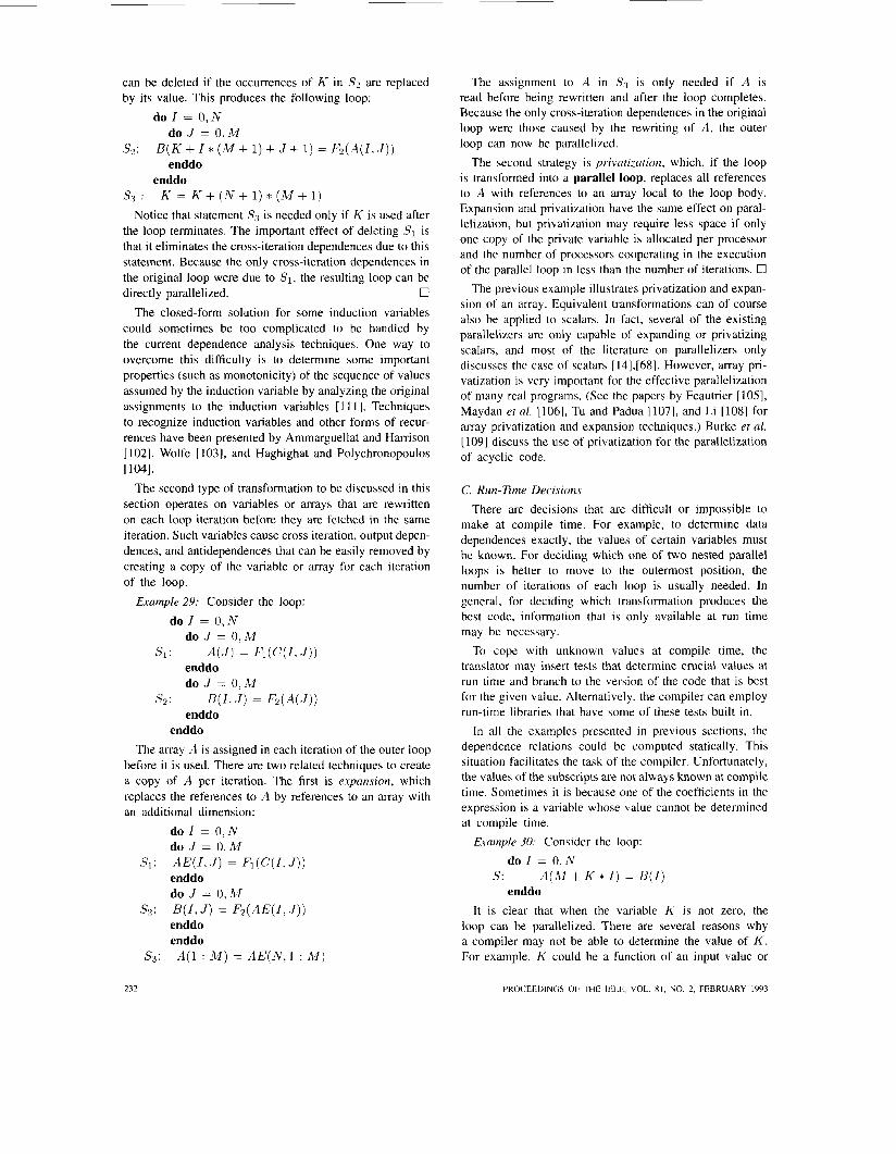
can be deleted if the occurrences of K in S2 are replaced by its value. This produces the following loop:

d o 1 = 0 , N do J = O,M

enddo S2: B ( K + I * ( M + 1) + J + 1) = F2(A(I. . J ) )

enddo S3 : K = K + ( N + 1 ) * ( M + 1 )

Notice that statement Ss is needed only if K is used after the loop terminates. The important effect of deleting SI is that it eliminates the cross-iteration dependences due to this statement. Because the only cross-iteration dependences in the original loop were due to S1, the resulting loop can be

The closed-form solution for some induction variables could sometimes be too complicated to be handled by the current dependence analysis techniques. One way to overcome this difficulty is to determine some important properties (such as monotonicity) of the sequence of values assumed by the induction variable by analyzing the original assignments to the induction variables [ 1 1 I]. Techniques to recognize induction variables and other forms of recurrences have been presented by Ammarguellat and Harrison [ 1021, Wolfe [ 1031, and Haghighat and Polychronopoulos [104].

The second type of transformation to be discussed in this section operates on variables or arrays that are rewritten on each loop iteration before they are fetched in the same iteration. Such variables cause cross iteration, output dependences, and antidependences that can be easily removed by creating a copy of the variable or array for each iteration of the loop.

directly parallelized. 0

Example 29: Consider the loop:

do .I = 0 , M

enddo

do I = 0 , N

Si: A ( J ) = Fl (C(1 .J ) )

do .I = 0 , M 5’2: B(1.J) = F2(A(J ) )

enddo enddo

The array A is assigned in each iteration of the outer loop before it is used. There are two related techniques to create a copy of A per iteration. The first is expansion, which replaces the references to A by references to an array with an additional dimension:

do I = 0. N do .I = O:M

enddo do J = 0 , M B(1, J ) = F2(AE(I, . I ) ) enddo enddo

Si: A E ( I , J ) = F1(C(I ,cJ))

S2:

5’3: A ( l : M ) = A E ( N , 1 : M )

The assignment to A in SH is only needed if A is read before being rewritten and after the loop completes. Because the only cross-iteration dependences in the original loop were those caused by the rewriting of A, the outer loop can now be parallelized.

The second strategy is privatization, which, if the loop is transformed into a parallel loop, replaces all references to A with references to an array local to the loop body. Expansion and privatization have the same effect on parallelization, but privatization may require less space if only one copy of the private variable is allocated per processor and the number of processors cooperating in the execution of the parallel loop in less than the number of iterations. 0

The previous example illustrates privatization and expansion of an array. Equivalent transformations can of course also be applied to scalars. In fact, several of the existing parallelizers are only capable of expanding or privatizing scalars, and most of the literature on parallelizers only discusses the case of scalars [ 14],[68]. However, array privatization is very important for the effective parallelization of many real programs. (See the papers by Feautrier [ 1051, Maydan et al. [ 1061, Tu and Padua [ 1071, and Li [ 1081 for array privatization and expansion techniques.) Burke et al. [ 1091 discuss the use of privatization for the parallelization of acyclic code.

C. Run-Time Decisions There are decisions that are difficult or impossible to

make at compile time. For example, to determine data dependences exactly, the values of certain variables must be known. For deciding which one of two nested parallel loops is better to move to the outermost position, the number of iterations of each loop is usually needed. In general, for deciding which transformation produces the best code, information that is only available at run time may be necessary.

To cope with unknown values at compile time, the translator may insert tests that determine crucial values at run time and branch to the version of the code that is best for the given value. Alternatively, the compiler can employ run-time libraries that have some of these tests built in.

In all the examples presented in previous sections, the dependence relations could be computed statically. This situation facilitates the task of the compiler. Unfortunately, the values of the subscripts are not always known at compile time. Sometimes i t is because one of the coefficients in the expression is a variable whose value cannot be determined at compile time.

Exumple 30: Consider the loop: do I = 0 . N

enddo 5’: A ( h l + K * I ) = B(1)

It is clear that when the variable K is not zero, the loop can be parallelized. There are several reasons why a compiler may not be able to determine the value of K . For example, K could be a function of an input value or

232 PROCEEDINGS OF THE IEEE, VOL 81, NO. 2, FEBRUARY 1993

t

0 1 2 3 4

Fig. 18. Dependence graph of loop in Example 31

the compiler may not be able to determine its value due to limitations of the analysis algorithms.

The strategy that is followed in cases like this is to generate conditional parallel code, known as two-version loops [ 1101, that is executed only when K is not zero:

if K = 0 then

else A ( M ) = B ( N )

parallel do I = 0, N

enddo A ( M + K * I ) = B ( I )

end if 0

Other cases more complex than the previous example may arise, and in some of these it is profitable to apply at run time some of the dependence tests described in Section 11. (See [ 11 11 for an example.) Multiple-version loops similar to the one used in the previous examples can be controlled by run-time dependence tests but also by other dynamic factors mentioned above. For example, the loop headers could be interchanged in several ways and one version selected for execution depending on the values of the loop limits.

Array subscripts could have a form that is impossible to analyze, using the dependence tests described in Section 11. However, if the subscript values are known before the loop starts execution, it is possible to determine at run time in which order to execute the loop in order to exploit some parallelism.

Example 31: Consider the loop: do I = 0 , 4

Si: A ( K ( I ) ) = B(1) 5'2: C ( I ) = A ( L ( I ) )

enddo The subscripts of the references to array A are themselves

array elements. If the values of K and L are not known at compile time, it is not possible to determine whether or not the loop can be parallelized. However, in many situations parallel execution of the loop would be possible. For example, if K =< 1,2 ,3 ,5 ,10 > and L =< 7,5 ,1 ,3 ,4 >, the iteration dependence graph would take the form shown in Fig. 18, from which it is clear that iterations 0,1, and 4 can execute in parallel in a first step, followed by the

0 A technique to handle, at run time, situations like the

one in the preceding example has been discussed by Zhu and Yew [ 1121. In this technique, the set of iterations that can execute in parallel and their order are computed every

parallel execution of iterations 2 and 3.

time the loop is executed. A second technique, proposed by Saltz et al. [113], assumes that the subscripts do not change between loop executions and therefore the subscript analysis is only needed the first time the loop is executed.

D. Issues in Non-Fortran languages 1) Pointer Analysis: Dependence analysis in the presence

of pointers has been found to be a particularly difficult problem. Programming languages such as C allow aliases to be created at any program point, and between memory locations allocated statically or dynamically. Much work has been done on this problem, though in general it remains unsolved. A common approach is to automatically infer the relationship between the pointers and their targets. For example, a compiler could infer that a pointer refers to a linear linked list (as opposed to a circular linked list), allowing more accurate dependence analysis during a list traversal. This approach has been taken by numerous researchers, with varying degrees of success [ 1 1414 1231; recursion and cyclic relationships have posed the greatest difficulty (the recent work of Deutsch [124] may prove more powerful). A related approach, originally focused on solving a different problem (automatic type inference or lifetime analysis, for example), can be used to provide alias information as well [125]-[127]; the viability of this approach has not been demonstrated. Finally, various language-based approaches [ 12814 1311 provide the compiler with additional information on which to base dependence decisions (or in the case of [132], represent a data structure in a more parallel form).

is seldom used today in numerical programs, partly because it is not part of the Fortran 77 standard. However, recursion is the most natural way to express some algorithms, especially nonnumerical algorithms.

We describe in this section a technique developed by Harrison [ 1331, called recursion splitting, which, although it was originally developed to parallelize Lisp programs, can be applied to programs in other languages including Fortran 90. Assume a function of the form:

2 ) Parallelization of Recursive Constructs: Recursion

function z ( P ) if q(P) then return(r(P))

return g(P, Y ) y = 4f(P>)

end Any recursive function can be cast into this form if q,

T , f , and g are chosen appropriately. Recursion splitting transforms the invocations to x (for example, z(P0) where Po could represent a sequence of parameters) into the expression

reduce(g, expand(Po,q, f, r ) )

where expand(P0, q , f, T ) returns the sequence

This sequence is just the value of the parameters in SUC- cessive invocations to 2; that is, pk = f(Pk-I). Also, m


is the depth of thg recursion; that is q(P,+l) is true and q(Pi) is false for i 5 m. It is easy to see that the value returned by the original function z is:

g(PO,...,9(P,-l,g(~,,r(~,,,+l))) .'.I which can be written as reduce(g, Po,. . . , PnE, r(P,+l)). Once the program has been written in this form, the reduce and expand functions can be parallelized.

Example 32: Consider the following function:

if A 5 B then return(C) return talc( t a k ( A - 1, B, C ) ,

function talc(A, B , C )

t&(B - 1, C, A) , talc(C - 1, A, B ) )

end This function can be cast into the form shown above in

several ways; one is: function t a k ( A , B , C )

if A 5 B then return(C)

return talc( Y, Y = tak(A - l ,B,C)

t~ lc (B - 1, C, A) , t ~ k ( C - 1, A, B ) )

end In the expandreduce form presented above, the function f corresponding to this version of tuk is just f ( A . B. C) = A - 1, B, C. Assuming that the original invocation to tulc is tuk(Ao, Bo, CO) and that A0 > Bo, then expand should generate the sequence:

Po = (Ao, Bo, CO), Pl = (Ao - 1, Bo, CO), . . . , Pnt (Bo, BO, CO)

which can be clearly computed in parallel. Also, the reduce function in this case involves two invocations of tuk for each Pi. Both of these invocations can be executed in parallel. 0

Iv . EFFECTIVENESS OF AUTOMATIC PARALLELIZATION

A. Introduction

Demonstrating the effectiveness of new approaches is a requirement in every scientific discipline. Effectiveness measures help the designer decide what new technology to adopt, what to set aside in favor of less complexity, and what topics need further study. This is particularly important in the case of parallelizing compilers, given the large number of possible transformations.

The value of effectiveness studies of traditional compiler technology is widely recognized, and there are a number of papers on the subject. For example, Cocke and Markstein [ 1341 reported the effectiveness of several traditional techniques such as common subexpression elimination, code motion, and dead code elimination.

Unfortunately, published studies on the effectiveness of parallelizing compilers are relatively sparse. The effective-

ness of new compiler techniques is usually demonstrated using simple and often artificial program segments that can be analyzed or transformed successfully. However, the papers introducing these new techniques also point out that more performance studies are necessary.

In this section we present first a survey of the available literature on the evaluation of instruction-level parallelism (Section IV-B) and loop-level parallelizing compilers (Sec- tion IV-C) followed in Section IV-D by a discussion of the implications of these evaluations.

B. Pe~ormance Evaluation of Instruction-Level Parallelism The current commercially available or soon-to-be-

available microprocessors have limited amounts of hardware parallelism. Furthermore, some of the production compilers used for these machines often lag behind the state of the art. Nevertheless, performance previously associated with supercomputers is becoming commonly available on these new processors. Thus, for example, the PA-RISC HP 730, achieves 75 SPECmarks, while the new DEC Alpha processor is projected to obtain 110 SPECmarks [ 135).

More fundamental studies that attempt to measure the potential of instruction-level transformations have also become available. Many of these studies assume some idealized circumstances, such as unlimited resources or complete compile-time knowledge of dependences and branches. An early study on numerical kernels by Nicolau and Fisher [ 1361 found an average of 90-fold parallelism available at the instruction level, given absolute dependence information and absolute branch prediction. The parallelism found was mainly limited by the problem size, which had to be kept small due to limitations of the experiment implementation.

In a more recent study Wall [ 1371 evaluated complete nu- meric and systems benchmarks under various dependence- analysis and branch-prediction conditions, ranging from idealized to realistic. The results showed instruction-level parallelism average factors of 7 for dynamic and 9 for static scheduling under idealized conditions, with factors of about 4-5 estimated to be achievable with state-of-the-art realistic compiler techniques.

Early efforts in instruction-level parallelism by Tjaden and Flynn [ 1381 and Riseman and Foster [ 1391 investigated the amounts of parallelism available at the machine instruction level for either static (compile-time) or dynamic (run- time) parallelism exploitation. The former study limited itself to finding parallelism within basic blocks,' and thus found only factors of 2-3 speedup over sequential execution. The latter study found significantly larger speedups (factors of 51 over sequential code, on average) but was based on a brute-force approach that involved cloning the hardware at each branch encountered and following all paths in parallel. The study concluded that dynamic

9 A reasonable restriction given that no global-i.e., beyond basic block boundaries-instruction-level parallelization techniques had been yet developed at the time.

234 PROCEEDINGS OF THE IEEE. VOL. 81. NO. 2, FEBRUARY 1993

exploitation of parallelism beyond basic blocks was impractical, as the hardware required to achieve significant speedups with the proposed approach was prohibitive. This study also confirmed the previous results regarding the small speedups achievable within basic blocks.

In more recent studies Ellis [41] and Lam [63] have taken into account the development of global instruction-level parallelization techniques. The former effort utilized trace scheduling in the context of simulated VLIW architectures and achieved speedups of over 10-fold over sequential code. The latter effort performed extensive experiments with software pipelining and hierarchical reduction” on the Warp machine. The results were very good in terms of the utilization of the machine, but the actual speedups were smaller (factors of three-fold over sequential) because of the resource limitations of the Warp hardware.

Other work has evaluated the applicability of instruction- level parallelism extraction techniques in systems and AI codes. Such codes are characterized by frequent and unpre- dictable control-flow. In experiments using a modification of percolation scheduling and a software pipelining scheme to generate code for a VLIW engine under construction at IBM T.J. Watson Labs, speedups of more than 10-fold versus the initial sequential code have been reported by Ebcioglu [140]. In a related paper Nakatani and Ebcioglu [141] showed that average speedups of 5.4-fold could still be obtained in systems and AI codes, even when percolation of operations is limited to a relatively small (moving) window in order to reduce code explosion and compilation- time. In an independent effort Potasman [53] evaluated the effect of percolation scheduling used in conjunction with software pipelining and various auxiliary techniques (e.g., renaming) on a variety of kernels from numerical as well as systems codes. Average speedups of 11-fold over sequential execution were obtained, given sufficient resources.

Perhaps the most robust results to date, using state- of-the-art compilation techniques for a relatively large instruction-level machine, come from the Multiflow Trace by Colwell et al. [42]. This paper reports five-fold to six-fold speedups on full scientific applications on a seven- functional-unit trace machine using their trace-scheduling compiler. This speedup was relative to a Vax 8700.” The paper also claims “based on experience with 25 million lines of scientific code” a speedup of two-fold to three- fold over “comparable” vector processors, but not enough information is provided to make an evaluation of this claim feasible. The code-size increase from trace scheduling and loop unrolling was reported to be approximately three-fold. An effective technique to further limit the code explosion in trace scheduling has also been reported by Gross and Ward [142].

‘OHierarchical reduction is a technique that combines branches of conditionals for the purpose of data and resource analysis. This allows the application of software pipelining techniques that normally work only on straight-line code, to code containing conditional control flow.

I ’ Although the the Vax 8700 and the multiflow trace have different organizations, the basic hardware of the two machines is roughly the same.

An evaluation of the dynamic exploitation of instruction- level parallelism was done by Butler et al. [ 1431, who report that with an issue rate of 8 instructions per cycle (and with a window-size limit placed on the total number of instructions currently under evaluation), speedups of 2-5.8 over sequential can be obtained on the SPEC benchmarks. Much larger potential parallelism (17-1 166fold) is found in these benchmarks if the issue and window-size limits are lifted (i.e., in an unrestricted (ideal) data-flow model).

C. Effectiveness of Loop Parallelizers Three groups of studies are presented next. First, in

Section IV-CI) we present two studies that evaluate several compilers according to the number of parallel loops that can be recognized as such. In Section IV-C2), we discuss comparisons of compilers based on the performance of the resulting codes on real machines. Next, in Section IV-C3), evaluations of the effectiveness of individual compilation techniques are presented. Finally, in Section IV-C4), we discuss several projects that, after studying the output of some parallelizers, conclude that there is much room for improvement in today’s parallelizers.

As will be seen below, the compilers most often evaluated are KAP and VAST. These are source-to-source parallelizing compilers developed by Kuck & Associates and Pacific Sierra Research, respectively. Also, there are a few evaluations of parallelizing compilers developed by individual computer companies. However, we should indicate that even though the evaluation reports do not always point this out, some of these compilers are based on VAST (e.g., Alliant FW8 optimizer, Cray Autotasking) or KAP (e.g., Alliant FW2800 optimizer).

I ) Recognizing Parallelism: One way to evaluate a parallelizing compiler is to count the number of program segments that can be parallelized. The two projects discussed here measure the number of do loops that the compilers under evaluation were able to vectorize totally or partially.

Detert [ 144,1451 used 101 short Fortran loops to evaluate the compilers of seven parallel machines. Callahan et al. [146] did a similar but more extensive study using 100 short loops. A total of 19 compilers and machines were evaluated. Both studies show that there is a wide variability in the capabilities of existing compilers. For example, in the second study, one of the compilers was only able to parallelize 24 loops, while others recognized as many as 69. Table 1 summarizes these results.

Data-dependence tests, as described in Section 11, are crucial for the successful recognition of parallel loops. Early evaluation work for these techniques was done by Shen et al. [147] who have analyzed subscript patterns that arise in real programs. Maydan et al. [19] and Goff et al. [20] present statistics on the success rates of data-dependence tests. Recently, Petersen and Padua [ 1481 have extended this work by relating these numbers to program performance of a suite of Benchmark programs.


TABLE I Number of Loops Vectorized Automatically. First Section: [I451 (101 Loops Total). Second Section: (1461 (100 Loops Total)

Machine Compiler Vectorized Partially Vectorized Not Vectorized

Alliant FW8

Convex Cl

Cray 2, Cray X-MP

Cray X-MP

ETA- 10

Fujitsu VP200

IBM 3090VF

Alliant FX/8

Amdahl VP-E Series

Ardent Titan- I

CDC Cyber 205

CDC Cyber 990E/995E

Convex C Series

Cray Series

CRAY X-MP

Cray Series

CRAY-2

ETA- 10

Gould NP1

Hitachi S-810/820

IBM 3090NF

Intel iPSC/2-VX

NEC SW2

scs-40

Stellar GS 1000

Unisys ISP

FX/Fortran V2.0.18

Fortran V 2.2

CFr 77 v1.2

CFT 1.15 BF 2

VAST-2 V 2.20H2

Fortran 77 V 1.2

Vs Fortran v 2.1.1

FXEortran V4.0

Fortran 77NP VIOL30

Fortran V 1 .0

VAST-2 V2.21

VFTN V2.1

FC 5.0

CF77 V3.0

CFT v1.15

cFr77 v3.0

CFT2 V3.la

FTN 77 V1.O

GCF 2.0

Fortran77/HAP V20-2B

VS Fortran V2.4

VAST-2 V2.23

Fortran77/SX V040

CFT x13g

Fortran77 prerelease

UFTN 4.1.2

76

81

69

75

71

79

59

68

62

62

62

25

69

69

50

50

27

62

60

67

52

56

66

24

48

67

14

I0

0

0

8

5

4

5

I I

6

5

I I

5

3

I

I

I

7

7

4

4

8

5

1

I I 13

I I

10

32

26

24

17

38

27

27

32

33

64

26

28

49

49

72

31

33

29

44

36

29

75

41

20

2) Comparing Performance Measurements: Other researchers have focussed on actual timing measurements of automatically parallelized code. Thus, Nobayashi and Eoyang [ 1491 evaluated several vectorizing compilers by translating a collection of program kernels onto three machines: Cray X-MP, Fujitsu VP, and NEC SX. They found that compilers that vectorize more loo<s do not necessarily produce faster code. They also show that kernel measurements can yield very divergent results. Table 2 summarizes one of the measurements, which compared the performance of the automatically restructured loops with that of hand-restructured loops and also shows the number of loops whose automatichand-optimized performance ratio is higher than the threshold shown in the table.

TABLE 2 Performance Ratio is higher than the Threshold in 11491

Number of Loops (out of 46) whose Automatic/Optimal

Threshold NEC SX Fujitsu VP Cray Cray X-MP X-MP C F r cFT77

90% 14 17 9 I I

80% 16 26 12 12

70% 18 26 15 15

Arnold [ 1501 reports performance improvements produced by KAP, VAST, and FTN200, the Fortran compiler of the Cyber 200 machines, on 18 Livermore Loops.

236 PROCEEDINGS OF THE IEEE, VOL. 81. NO. 2, FEBRUARY 1993

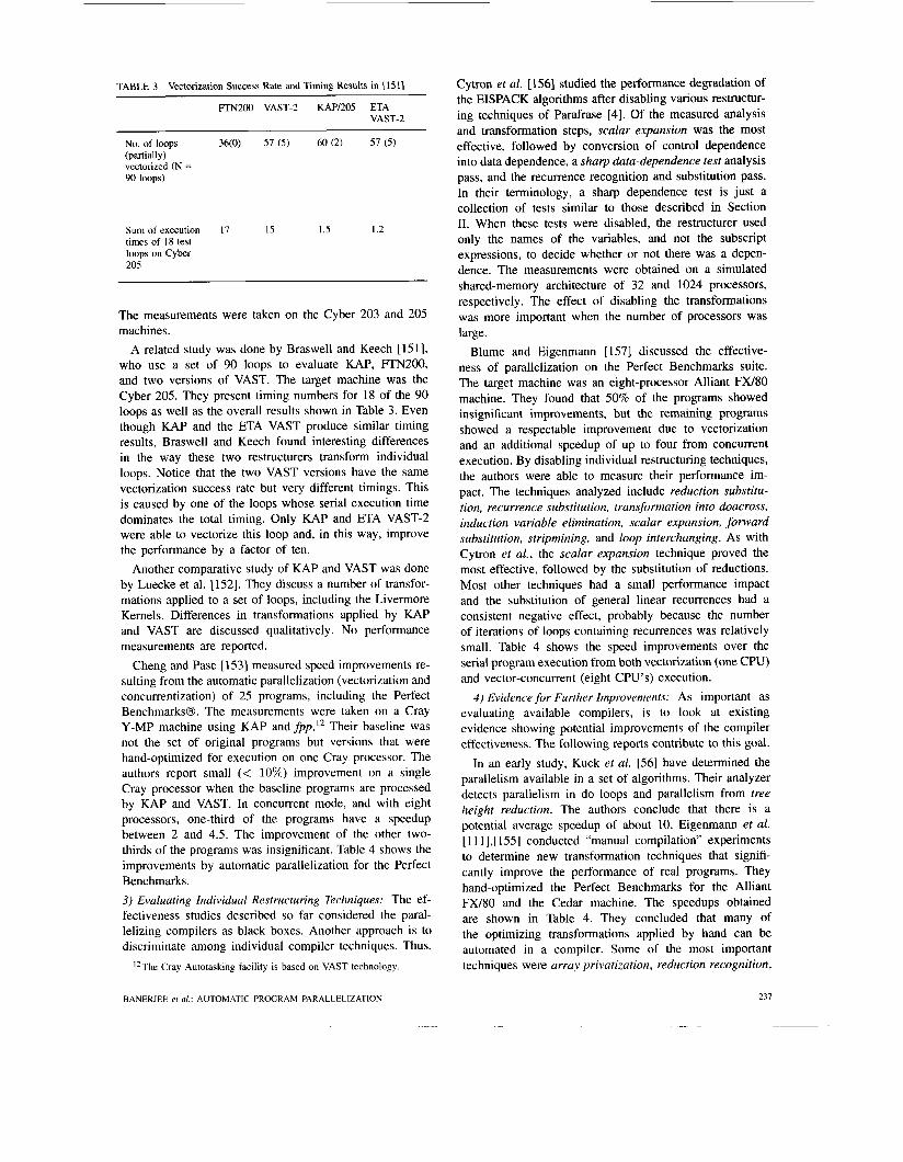
TABLE 3 Vectorization Success Rate and Timing Results in [ 15 11

FI?r1200 VAST-2 KAPl205 ETA VAST-2

No. of loops 36(0) 57 ( 5 ) 60 (2) 57 ( 5 ) (partially) vectorized (N = 90 loops)

Sum of execution 17 15 times of 18 test loops on Cyber 205

1.5 1.2

The measurements were taken on the Cyber 203 and 205 machines.

A related study was done by Braswell and Keech [151], who use a set of 90 loops to evaluate KAP, FTN200, and two versions of VAST. The target machine was the Cyber 205. They present timing numbers for 18 of the 90 loops as well as the overall results shown in Table 3. Even though KAP and the ETA VAST produce similar timing results, Braswell and Keech found interesting differences in the way these two restructurers transform individual loops. Notice that the two VAST versions have the same vectorization success rate but very different timings. This is caused by one of the loops whose serial execution time dominates the total timing. Only KAP and ETA VAST-2 were able to vectorize this loop and, in this way, improve the performance by a factor of ten.

Another comparative study of KAP and VAST was done by Luecke et al. [152]. They discuss a number of transformations applied to a set of loops, including the Livermore Kernels. Differences in transformations applied by KAP and VAST are discussed qualitatively. No performance measurements are reported.

Cheng and Pase [ 1531 measured speed improvements resulting from the automatic parallelization (vectorization and concurrentization) of 25 programs, including the Perfect Benchmarks@. The measurements were taken on a Cray Y-MP machine using KAP andfpp.12 Their baseline was not the set of original programs but versions that were hand-optimized for execution on one Cray processor. The authors report small (< 10%) improvement on a single Cray processor when the baseline programs are processed by KAP and VAST. In concurrent mode, and with eight processors, one-third of the programs have a speedup between 2 and 4.5. The improvement of the other two- thirds of the programs was insignificant. Table 4 shows the improvements by automatic parallelization for the Perfect Benchmarks. 3) Evaluating Individual Restructuring Techniques: The effectiveness studies described so far considered the parallelizing compilers as black boxes. Another approach is to discriminate among individual compiler techniques. Thus,

”The Cray Autotasking facility is based on VAST technology.

BANERJEE er al.: AUTOMATIC PROGRAM PARALLELIZATION

Cytron et al. [ 1561 studied the performance degradation of the EISPACK algorithms after disabling various restructuring techniques of Parafrase [4]. Of the measured analysis and transformation steps, scalar expansion was the most effective, followed by conversion of control dependence into data dependence, a sharp data-dependence test analysis pass, and the recurrence recognition and substitution pass. In their terminology, a sharp dependence test is just a collection of tests similar to those described in Section 11. When these tests were disabled, the restructurer used only the names of the variables, and not the subscript expressions, to decide whether or not there was a dependence. The measurements were obtained on a simulated shared-memory architecture of 32 and 1024 processors, respectively. The effect of disabling the transformations was more important when the number of processors was large.

Blume and Eigenmann [ 1571 discussed the effectiveness of parallelization on the Perfect Benchmarks suite. The target machine was an eight-processor Alliant FW80 machine. They found that 50% of the programs showed insignificant improvements, but the remaining programs showed a respectable improvement due to vectorization and an additional speedup of up to four from concurrent execution. By disabling individual restructuring techniques, the authors were able to measure their performance impact. The techniques analyzed include reduction substitution, recurrence substitution, transformation into doacross, induction variable elimination, scalar expansion, forward substitution, stripmining, and loop interchanging. As with Cytron et al., the scalar expansion technique proved the most effective, followed by the substitution of reductions. Most other techniques had a small performance impact and the substitution of general linear recurrences had a consistent negative effect, probably because the number of iterations of loops containing recurrences was relatively small. Table 4 shows the speed improvements over the serial program execution from both vectorization (one CPU) and vector-concurrent (eight CPU’s) execution.

4 ) Evidence for Further Improvements: As important as evaluating available compilers, is to look at existing evidence showing potential improvements of the compiler effectiveness. The following reports contribute to this goal.

In an early study, Kuck et al. [56] have determined the parallelism available in a set of algorithms. Their analyzer detects parallelism in do loops and parallelism from tree height reduction. The authors conclude that there is a potential average speedup of about 10. Eigenmann et al. [ 11 1],[ 1551 conducted “manual compilation” experiments to determine new transformation techniques that significantly improve the performance of real programs. They hand-optimized the Perfect Benchmarks for the Alliant FX/80 and the Cedar machine. The speedups obtained are shown in Table 4. They concluded that many of the optimizing transformations applied by hand can be automated in a compiler. Some of the most important techniques were array privatization, reduction recognition,

231

TABLE 4 programs on Cray Y-MP 11531. Third and fourth line: Improvements over serial program execution on Alliant FX8 [ 1541. Fifth line: manual improvements over serial program execution on Alliant FX8 [ 1551

Performance improvements of the Perfect Benchmarks. First two lines: Improvements over manually vector-optimized

ADM ARCZD B D N A DYFESM F L 0 5 2 MDG MG3D OCEAN QCD SPEC77 SPICE TRACK TRFD

1 1 1 Vectorized (Y-MP, 1.2 1 1 1 1 1 0.9 1.2 I 1 one CPU)

Vector-concurrent I 3.1 1 I .2 2.5 1 0.9 1 . 1 I 1.2 1 1 1 (Y-MP, eight CPU’s)

Vectorized (FW8, 1.1 2.0 1.1 3.6 3.4 1.2 2.3 1.3 1.2 2.2 1.1 1.1 2.8 one CPU)

Vector-concurrent 1.3 8.0 3.3 4.3 10.2 1.1 1.6 1.3 1.2 2.3 1.1 1.0 2.2 (FX/8, eight CPU’s)

Manually improved 7.5 10.5 4.2 7.7 16 5.5 4.4 8.3 7.0 5.5 5.1 14.3 (FX/8, eight CPU’s)

and recognition of complex forms of induction variables. They also pointed out the need for advanced interprocedural analysis techniques. It is worth noting that many of the transformations discussed in Section 111 were not found necessary to obtain good performance. Most of the loops could be transformed into completely parallel forms (i.e., vector and parallel dos without synchronization) after the transformations just mentioned were applied.

Singh and Hennessy [I581 studied the limitations of automatic parallelization using three scientific applications. They found that the time-consuming loop nests are often complex and require more sophisticated analysis and data restructuring. Recommendations for further development of automatic parallelization technology are given. These include advances in symbolic data-dependence analysis, dataflow and interprocedural analysis, and privatiza- tiodexpansion of data structures.

Petersen and Padua 11 591 have compared the parallelism found by compilers to an estimated maximum parallelism and derived potential compiler improvements. The compiler used is KAP/Concurrent. The maximum parallelism is measured by instrumenting the program so that the execution can be simulated for an ideal machine, taking into account all essential data dependences. It is found that both maximum and compiler-extracted parallelism vary widely. The authors conclude that there are potential improvements for compilers in handling unknown values at compile time, subscripted subscripts, non-parallelizable statements, and subroutine calls.

D. Discussion Table 5 summarizes the reports on loop-level paralleliza-

tion described above, including the test suites, machines, compilers, and the measurements used in each study. The earlier compiler effectiveness studies measured how successfully individual loops were parallelized. As shown in Tables 1-3, these studies agree that, under this criterion, automatic parallelization is relatively successful. However, even though many of these loops are extracted from real

programs, the measurements of how effectively they can be parallelized do not necessarily predict the behavior on real programs. In fact, recent program-level studies have drawn different conclusions: Many real programs are not improved by existing compilers. This does not mean that parallelizers fail all the time, and in fact there are some real programs on which parallelization does a very good job. The two most extensive measurements of the effectiveness of parallelization on real codes are presented in [153] and [ 1571. Both studies report small improvements from automatic parallelization for a majority of the programs studied. However, i t should be remembered that these two studies use different types of programs. Cheng and Pase [ 1531 start with hand-optimized codes whereas [I571 starts with unmodified programs. This is probably why [157] reports a higher effectiveness in a few programs whereas [ 1531 sometimes shows performance degradations. The (additional) automatic vectorization done in the latter study leads to little or even negative improvement. Apparently the automatic vectorization could not find more parallelism than the previous manual optimization, but introduced some overhead. It is not reported to what extent manual vector optimizations were applied.

Another important result is that many restructuring techniques were found ineffective [ 1571, presumably because many of the most time-consuming loops of the programs could not be parallelized. However, it was also shown that these loops can potentially be transformed into parallel code [ 1551 by advanced techniques. Hence, the existing techniques may become more effective once more powerful complementary compiler technology is developed.

The evaluation papers on instruction-level parallelism (Section IV-B) have shown that corresponding compiler technology has been developed that is able to successfully exploit multiple functional units. However, there is room for studies that evaluate this technology more comprehensively.

There exists evidence for potential improvements of parallelizing compilers. It was given by analyzing real program patterns and deriving new compiler capabilities [ 1611, by

238 PROCEEDINGS OF THE IEEE. VOL 81. NO. 2. FEBRUARY 1093

TABLE 5 Summary of Compiler Effectiveness Studies

Study Test Suite Measures Machines Compilers

K A P V N T S I F

X

X

X

X

X X

X X

X X

X X

X X X

X X

X X X

X

X

X X

X X

X

X

X

si m u 1 at e d

Cyber 20315

simulated

simulated

see Table 1

Cyber 205

see Table 1

NAS 160

see Table 2

Alliant FX/8

Cray Y-MP

X Alliant FW8

X FW8, Cedar

X simulated

FrN200, U P , VAST

Parafrase

Parafrase

FrN200, KAP, VAST

KAP, VAST

U P , VAST

U P , fPP

VAST

KAP

KAP

Note: test suite: K=Kemels; A=Algorithms; P=Application programs. Measures: V=shows rate of successfully vectorized loops; N=compares performance numbers of different compilers; T=compares transformations of different compilers; S=shows speedups due to automatic parallelization; I=evaluates individual compiler techniques; and F=discusses future compiler improvements.

optimizing programs manually and discussing the automata- bility of the transformations applied [ 11 1],[ 1551, and by comparing “best” parallelism to that found by compilers [ 1591 and deriving new restructuring capabilities. At the instruction-level potential advances have been pointed out in increasing the window size when dynamically exploiting parallelism [ 1431.

The measurements have pointed out both success and limitations of available automatic parallelizers. Improve- ments are necessary to make restructurers consistently useful tools in multiprocessor environments. The reports on potential improvements do not prove that future compilers will be much more effective; however, they give reasonable indication that significant performance improvements are possible and-perhaps more important-that efforts are worthwhile to search for and implement new, more powerful automatic parallelization techniques.

V. CONCLUSIONS Many program analysis and transformation techniques

for program parallelization have been developed, primarily

during the last decade. A program calculus is now emerging that allows the formal analysis of these transformations as well as the development of new powerful transformations. However, these techniques are only as good as their impact on the performance of the target program. As discussed in Section IV-D, there is a need for more experimental evaluation and analysis of the nature of real programs.

The ultimate goal of research in program parallelization is to develop a methodology that will be effective in translating a wide range of sequential programs for use with several classes of scalable parallel machines. Although it is not clear how close we are to that goal, it is clear is that we are not there yet and that our research effort must continue because of the great impact that effective parallelizers are bound to have on the ordinary users’ acceptance of parallel machines.

ACKNOWLEDGMENT The authors wish to thank William Blume, Keith Faigin,

John Grout, Jay Hoeflinger, Jose Moreira, Paul Petersen, and Steve Weatherford for their many useful suggestions.


REFERENCES

[ I ] D. J. Kuck, R. H. Kuhn, D. A. Padua, B. Leasure, and M. Wolfe, “Dependence graphs and compiler optimizations,” in Proc. 8th ACM Symp. on Principles of Programming Languages, Jan. 1981, pp 207-218.

121 D. Padua and M. Wolfe. “Advanced comoiler ootimization for _ _ supercomputers,” CACM, vol. 29, no. 12,‘pp. 11’84-1201, Dec. 1986.

[3] J. Allen and K. Kennedy, “Automatic translation of Fortran programs to vector form,” ACM Trans. on Programming Languages and Systems, vol. 9, no. 4, pp. 491-542, Oct. 1987.

[4] D. J. Kuck, R. H. Kuhn, B. Leasure, and M. Wolfe, “The structure of an advanced vectorizer for pipelined processors,” in Proc. COMPSAC 80, The 4th Int’l. Computer Software and Applications Con$, Oct. 1980, pp. 709-715.

[5] J.R. Allen and K. Kennedy, “Pfc: A program to convert fortran to parallel form,” in Supercompurers: Design and Ap- plicationsNew York: IEEE Computer Society Press, 1985, pp. 186-205.

161 F. Allen, M. Burke, P. Charles, R. Cytron, and J. Ferrante, “An overview of the PTRAN analysis system for multiprocessing,” in Proc. Int. Con$ on Supercomputing, 1987, pages 194-2 1 1.

[7] C. Polychronopoulos, M. Girkar, M. Reza Haghighat, C.-L. Lee, B. Leung, and D. Schouten, “Parafrase-2: A new generation parallelizing compiler,” Int. J. High Speed Computing, vol. I , no. I , pp. 45-72, May 1989.

[S] R. Cytron, J. Ferrante, and V. Sarkar, “Experiences using control dependence in PTRAN,” in Languages and Compilers for Parallel Computing. Cambridge, MA: MIT Press, 1990, pp. 186-212.

[9] D. Knuth, The Art of Computer Programming. Vol. 2: Seminu- mericul Algorithms.

[ I O ] U. Banerjee, Dependence Analysis for Supercomputing. Nor- well, MA: Kluwer Academic Publishers, 1988.

[ I I] -, “Speedup of ordinary programs,” PhD thesis, Univ. of Illinois at Urbana-Champaign, Dept. of Computer Sci., Oct. 1979.

[ 121 M. Wolfe and U. Banerjee, “Data dependence and its application to oarallel orocessing,” Int. J . Parullel Propramminp. vol. 16.

Reading, MA: Addison-Wesley, 198 I .

no.. 2, pp. i37-178,”Apr. 1987. 1131 U. Baneriee. “Data deoendence in ordinarv o r o m “ n ’ Mas- .~ + . -

ter’s thesis, Univ. of Illinois at Urbana-Champaign, Dept. of Computer Sci., Nov. 1976.

[ 141 M. Wolfe, Optimizing Supercompilers for Supercomputers. Cambridge, MA: MIT Press, 1989.

[ 151 A. Schrijver, Theory <$Linear and Integer Programming. New Yrok: John Wiley, 1987.

[I61 2. Li, P. Yew, and C. Zhu, “An efficient data dependence analysis for parallelizing compilers.” IEEE Trans. Parallel and Distributed Systems, vol. 1 , no. I , pp. 26-34, Jan. 1990.

[ 171 X. Kong, D. Klappholz, and K. Psarris, “The i test: An improved dependence test for automatic parallelization and vectorization,” IEEE Trans. Parallel and Distributed Systems, vol. 2, no. 3, July 1991.

[I81 William Pugh, “the Omega test: A fast and practical integer programming algorithm for dependence analysis,’’ in Proc. Supercomputing’YI, Nov. 1991.

[19] D. Maydan, J. Hennessy, and M. Lam, “Efficient and exact data dependence analysis,” in Proc. ACM SICPLAN 9 1 Conf: on Programming Language Design and Implementation, Toronto, June 1991.

(201 G . Goff, K. Kennedy, and C. Tseng, “Practical dependence testing,” in Proc. ACM SIGPLAN ‘91 Conj on Programming Language Design and Implementation, Toronto, June 199 I .

[21] C. A. Huson, “an in-line subroutine expander for parafrase,” Master’s thesis, Univ. of Illinois at Urbana-Champaign, Dept. of Computer Sci., Dec. 1982.

[22] K. Cooper and K. Kennedy, “Efficsnt computation of flow in- sensitive interprocedural summary information,” in Proc. ACM SlCPLAN’84 Symp. on Compiler Construction. SICPLAN No- tices , vol. 19, no. 6, June 1984.

1231 R. Triolet. F. Irigoin, and P. Feautrier, “Direct parallelization of call statements, in Proc. ACM SIGPLAN’86 Symp. on Compiler Construction, SIGPLAN Notices, vol. 21, no. 7, June 1986.

[24] M. Burke and R. Cytron, “Interprocedural dependence analysis and parallelization,” in Proc. ACM SIGPLAN’86 Symp. on Compiler Construction, SICPLAN Notices, vol. 21, no. 7, June 1986.

[25] Z. Li and P.-C. Yew, “Efficient interprocedural analysis for program parallelization and restructuring,” Proc. ACM/SIGPLAN PPEALS, July 1988, pages 85-99.

[26] R. A. Towle, ”Control and data dependence for program transformations,” PhD thesis, Univ. of Illinois at Urbana-Champaign, Dept. of Computer Sci., Mar. 1976.

[27] J. Ferrante, K. J. Ottenstein, and J. D. Warren, “The program dependency graph and its uses in optimization,” ACM Trans. Programming Languages und Systems, vol. 9, no. 3, pp. 3 19-349, June 1987.

[28] J. R. Allen and K. Kennedy, “Conversion of control dependence to data dependence,” in Proc. 10th ACM Symp. on Principles of Programming Languuges, Jan. 1983.

[29] K. Pingali, M. Beck, R. Johnson, M. Moudgill, and P. Stodghill, “Dependence flow graphs: an algebraic approach to program dependencies” n Proc. 18th ACM Symp. on Principles of Pro- gramming Languages, Jan. 1991, pp. 67-78..

[30] M. Girkar and C. D. Polychronopoulos, “The HTG: an intermediate representation for programs based on control and data dependences,” l E E E Truns. Parullel and Distributed Systems, vol. 3, no. 2, pp. 166-178, Mar. 1992.

[311 Y. Wu and T. Lewis, “Parallelizing WHILE loops,” in Proc. 1YYO In?. Conj on Purallel Processing, St. Charles, Ill., Aug 13-17, 1990, pp. 1-8.

[32] W. Ludwell Harrison, “Compiling lisp for evaluation on a tightly coupled multiprocessor,” Technical Report 565, Univ. of Illinois at Urbana-Champaign, Center for Supercomputing Res. & Dev., Mar. 1986.

[ 3 3 ] E. Dijkstra, “Co-operating sequential processes,” in Progrum- ming Languages.

1341 E. Coffman and P. Denning, Operating Systems Theory. En- glewood Cliffs, NJ: Prentice-Hall, 1973.

[35] D. D. Gajski, D. J. Kuck, and D. A. Padua, “Dependence driven computation,” in Proc. COMPCON 81 Spring Computer Con$, Feb. 1981, pp. 168-172..

[36] S. Midkiff and D. Padua, “Compiler algorithm for synchronization,” IEEE Tram. Comput.. vol. C-36. no. 12, pp. 1485-1495, 1987.

[37] H. Kasahara, H. Honda, A. Mogi, A. Ogura, K. Fujiwara, and S. Narita, “A multi-grain parallelizing compilation scheme for OSCAR (optimally scheduled advanced multiprocessor),” in Languages and Compilers for Parallel Computing, Lecture Notes in Comp. Sci., Springer Verlag, 1992.

[38] M. Girkar and C. Polychronopoulos, “Optimization of datdcontrol conditions in task graphs,” in Languages and Compilers for Parallel Coniputing, Lecture Notes in Computer Science. New York: Springer-Verlag, 1992.

[39] J. Fisher, “Trace scheduling: A technique for global microcode compaction.” IEEE Truns. Computers, vol. C-30, no. 7, pp. 478490, July 1981.

[40] J. Fisher, J . Ellis, J . Ruttenberg, and A. Nicolau, “Parallel processing: A smart compiler and a dumb machine,” in Proc. 1984 SICPLAN Symp. on Compiler Construction, June 1984,

[41] J. Ellis, “Bulldog: A compiler for VLIW architectures,” Ph.D. thesis, Yale Univ., Department of Comput. Sci., Feb. 1985.

[42] R. Colwell, R. Nix, J. O’Donnell, D. Papworth, and P. Rodman, “A VLIW architecture for a trace scheduling compiler,” in Proc. Second lnt. Cot$ on Architecturul Support for Programming Languuges and Operating Systems, Oct. 1987.

[43] A. Nicolau, “Parallelism, memory anti-aliasing, and correctness for trace scheduling compilers,” Ph.D. thesis, Yale Univ., 1984.

(441 J. L. Linn, “Srdag CompAction: A generalization of trace scheduling to increase the use of global context information,” in Proc. 16th Annual Workshop on Microprogramming, Oct. 1983.

1451 R. Gupta and M. Soffa, “Region scheduling,” in Proc. 2nd Int. Con5 on Supercomputing, May 1987.

(461 Y. Patt and W. W. Hwu, “HPSm a high performance restricted data flow architecture having minimal functionality,” in The 13th Annual Int. Symp. Comput. Arch. Conj Proc., June 1986, p. 297.

1471 P. P. Chang, S. A. Mahlke, W. Y. Chen, N. J. Warter, and W. W. Hwu, “IMPACT: An architectural framework for multiple instruction issue processors,” In Conj Proc. 18th Annual Int. Symp. Comput. Arch., May 1991, p. 266.

[48] A. Nicolau, “Uniform parallelism exploitation in ordinary programs,” in Proc. 1985 Int. Con$ Parullel Processing, Aug. 1985,

New York: Academic, 1968, pp. 43-1 12.

pp. 3 7 4 7 .

pp. 614-618.

240 PROCEEDINGS OF THE IEEE, VOL 81, NO 2 , FEBRUARY 1993

[49] A. Aiken and A. Nicolau, “A development environment for horizontal microcode,” IEEE Trans. Sofhvare Eng., vol. 14, no. 5 , pp. 584-594, May 1988.

[50] A. Aiken, “Compaction-based parallelization,” Ph.D. thesis, Come11 Univ., Dept. of Comput. Sci., 1988.

[51] K. Ebcioglu, “A compilation technique for software pipelining of loops with conditional jumps,’’ in Proc. 20th Annual Workshop on Microprogramming, December 1987, pp. 69-79.

[52] K. Ebcioglu and A. Nicolau, “A global resource-constrained parallelization technique,” in Proc. ACM SIGARCH ICs-89: Int. Con$ on Supercomputing, Crete, Greece, June 1989.

[53] R. Potasman, “Percolation-based compiling for evaluation of parallelism and hardware design tradeoffs,” Ph.D. thesis, Univ. of California, Irvine, Dec. 1991.

[54] C. Polychronopoulos, “Compiler optimizations for enhancing parallelism and their impact on architecture design,” IEEE Trans. computers, vol. C-37, no. 8, pp. 991-1004, Aug. 1988.

[55] D. J. Kuck, The Structure of Computers and Computations. New York: John Wiley, vol. 1, 1978.

[56] D. Kuck, P. Budnik, S-C. Chen, Jr., E. Davis, J. Han, P. Kraska, D. Lawrie, Y. Muraoka, R. Strebendt, and R. Towle, “Mea- surements of parallelism in ordinary FORTRAN programs,” Computer, vol. 7, no. 1, pp. 3 7 4 6 , Jan. 1974.

[57] A. Aiken and A. Nicolau, “Perfect pipelining: A new loop parallelization technique,” in Proc. 1988 European Symp. on Programming, 1988, pp. 221-235.

[58] U. Schwiegelshohn, F. Gasperoni, and K. Ebcioglu, On “Opti- mal loop parallelization,” Technical Report, IBM T.J. Watson Research Center, Yorktown Hts., NY, 1989.

[59] P. Kogge, “The microprogramming of pipelined processors,” in Proc. 4th Annual Int. Symp. on Comput. Architecture, 1977.

[60] A. Charlesworth, “An approach to scientific array processing: The architectural design of the AP-120bFPS- 164 family,” IEEE Computer, col. C-14, no. 3, pp. 18-27, 1981.

[61] R. Touzeau, “A Fortran compiler for the FPS-I64 scientific computer,” in Proc. 1984 ACM SIGPLAN Symp. on Compiler Construction, June 1984, pp. 48-57.

[62] B. Rau and C. Glaeser, “Some scheduling techniques and an easily schedulable horizontal architecture for high performance scientific computing,” in Proc. 14th Annual Workshop on Mi- croprogramming, Oct. 1981, pp. 183-198.

[63] M. Lam, ”A systolic array optimizing compiler,” Ph.D. thesis, Camegie Mellon Univ., 1987.

[64] -, “Software pipelining: An effective scheduling technique for VLIW machines,” in Proc. SIGPLAN’88 Con$ on Program- ming Language Design and Implementation, June 1988.

[65] B. Su, S. Ding, and J. Xia, “GURPR-a method for global software pipelining,” in Proc. 20th Annual Workshop on Micro- programming, pp. 88-96, Dec. 1987.

[66] Y. Muraoka, ”Parallelism exposure and exploitation in programs,” Ph.D. thesis, Univ. of Illinois at Urbana-Champaign, Dept. of Comput. Sci., Feb. 1971.

[67] U. Banerjee, S. C. Chen, D. J. Kuck, and R. A. Towle, “Time and parallel processor bounds for Fortran-like loops,” IEEE Trans. Computers, vol. C-28, no. 9, pp. 660-670, Sept. 1979.

[68] H. Zima, Supercompilers for Parallel and Vector Computers. New York ACM Press, 1991.

[69] K. Kennedy and K.S. McKinley, “Loop distribution with arbitrary control flow,” in Proc. Supercomputing ’90, IEEE Com- puter Society Press, Nov. 1990, pp. 407-417.

[70] D. J. Kuck and D. A. Padua, “High-speed multiprocessors and their compilers,” Proc. 1979 Int. Con$ on Parallel Processing,

[71] D. A. Padua, D. J. Kuck, and D. H. Lawrie, “High-speed multiprocessors and compilation techniques,” Special Issue on Parallel Processing, IEEE Trans. on Computers, vol. C-29, no. 9, pp. 763-776: Sept. 1980.

[72] R. G. Cytron, Compile-time scheduling and optimization for asynchronous machines,” Ph.D. thesis, Univ. of Illinois at Urbana-Champaign, Dept. of Comput. Sci., Oct. 1984.

[73] -, “Doacross: Beyond vectorization for multiprocessors,” in Proc. Int. Con$ on Parallel Processing, 1986, pp. 836844.

[74] D. A. Padua, “Multiprocessors: discussion of some theoretical and practical problems,” Ph.D. thesis, Univ. of Illinois at Urbana-Champaign, Dept. of Computer Sci., Oct. 1979.

[75] Zhiyuan Li and Walid Abu-Sufah, “On reducing data synchronization in multiprocessed loops,” IEEE Trans. Computers, vol. C-36, no. 1, pp. 105-109, Jan. 1987.

Aug. 1979, pp. 5-16.

[76] V. Krothapalli and P. Sadayappan, “Removal of redundant dependences in DOACROSS loops with constant dependences,” IEEE Trans. Parallel Distributed Syst., vol. 2, no. 3, pp.

[77] R. Allen, D. Callahan, and K. Kennedy, “Automatic .decompo- sition of scientific programs for parallel execution,” in Pmc. Fourteenth Annual ACM Symp. on Principles of Programming Languages, Jan. 1987, pp. 63-76.

[78] M. Wolfe, “Advanced loop interchanging,” in Proc. 1986 Int. Con$ on Parallel Processing, St. Charles, Ill., Aug. 1986, pp. 536-543.

[79] J. Allen and K. Kennedy, “Automatic loop interchange,” in Proc. 1984 SIGPLAN Symp. Compiler Construction, vol. 19, June 1984, pp. 233-246.

[80] L. Lamport, “The parallel execution of DO loops,” Comm. of the ACM, vol. 17, no. 2, pp. 83-93, Feb. 1974.

[81] U. Banerjee, “Unimodular transformations of double loops” in Advances in Languages and Compilers for Parallel Processing Cambridge, MA: MIT Press, 1991, pp 192-219.

[82] M.E. Wolf and M. Lam, “A data locality optimizing algorithm,” in SIGPLAN NOTICES: Proceedings of the ACM SIGPLAN 91 Con$ on Programming Language Design and Implementation, Toronto, Ontario, ACM Press, June 1991, pp. 30-44.

[83] W. Shang and J. Fortes, “Time optimal linear schedules for algorithms with uniform dependencies,” IEEE Trans. Computers, vol. 40, no. 6, pp. 723-742, June 1991.

[84] J.-K. Peir and R. Cytron, “Minimum distance: A method for partitioning recurrences for multiprocessors,” in Proc. 1987 Int. Con$ on Parallel Processing, Pennsylvania State University Press, 1987, pp. 217-241.

[85] E. H. D’Hollander, “Partitioning and labeling of loops by unimodular transformations,” IEEE Trans. Parallel Distributed Syst., vol. 3, no. 4, pp. 465476, 1992.

[86] P. Tang, P.-C. Yew, and C.-Q. Zhu, “Impact of self-scheduling orders on performance,” Proc 1988 Int. Conf: on Supercomput- ing, St. Malo, France, July 1988, pp. 593-603.

[87] D. Loveman, “Program improvement by source-to-source transformation,” J. ACM, vol. 24, no. I , pp. 121-145, Jan. 1977.

[88] C. Polychronopoulos, “Loop coalescing: A compiler transformation for parallel machines,” in Proc. 1987 Int. Con$ Parallel Processing, St. Charles, Ill. August 1987, pages 235-242.

[89] W. Abu-Sufah, D. J. Kuck, and D. H. Lawrie, “On the performance enhancement of paging systems through program analysis and transformations,” IEEE Trans. Computers, vol. C-30, no. 5 , pp. 341-356, May 1981.

[90] A. McKellar and Jr. E. Coffman, “Organizing matrices and matrix operations for paged memory systems,” Comm. ACM,

[91] W. Jalby and U. Meier, “Optimizing matrix operations on a parallel multiprocessor with a memory hierarchy,” in Pro 1986 Int. Con$ Parallel Processing, St. Charles, Ill., Aug. 1986, pp. 4 2 9 4 3 2.

1921 M.J. Wolfe, “More iteration space tiling,” in Proc. Supercom- puling ’89, Reno, Nevada, Nov. 13-17, 1989, pp. 655-664.

[93] F. Irigoin and R. Triolet, “Supemode partitioning,” in Proc. Fifreenth Annual ACM Symp. on Principles of Programming Languages, Jan. 1988, pp. 319-329.

[94] C. Ancourt and F. Irigoin, “Scanning polyhedra with do loops,” in Proc. Third ACM SIGPLAN Symp. on Principles and Practice of Parallel Programming (PPOPP), Apr. 1991, pp. 39-50.

[95] R. Schreiber and J. Dongma, “Automatic blocking of nested loops,” Technical report, RIACS, Aug. 1990.

[96] R. Cytron, S. Karlovsky, and K. McAuliffe, “Automatic management of programmable caches,” in Proc. 1988 Int. Con$ Parallel Processing, St. Charles, Ill., Aug. 1988, pp. 229-238.

[97] E. H. Gomish, E. D. Granston, and A. V. Veidenbaum, “Compiler-directed data prefetching in multiprocessors with memory hierarchies,” in Proc. Int. Con$ Supercomputing, vol. I , June 1990, pp. 342-353.

[98] D. Callahan, K. Kennedy, and A. Porterfield, “Software prefetching,” in Proc. Fourth Int. Con$ Architectural Support for Programming Languages and Operating Systems, Apr. 199 1, pp. 40-52.

[99] E. Damell, J. M. Mellor-Crummey, and K. Kennedy, “Auto- matic software cache coherence through vectorization” in Pro. Int. Con$ Supercomputing, 1992, pp. 129-139.

[ 1001 A. Aho and J. Ullman, The Theory ofparsing, Translation, and Compiling.

281-289, July 1991.

vol. 12, pp. 153-165, 1974.

Englewood Cliffs, NJ: Prentice-Hall, 1973.

BANERJEE et al.: AUTOMATIC PROGRAM PARALLELIZATION 24 I

1011 R. Eigenmann, J. Hoeflinger, C . Jaxon, and D. Padua, “Cedar Fortran and its restructuring compiler,” in Advances in Lan- guages and Compilers f o r Parallel Processing. Cambridge, MA: MIT Press, 1991, pp. 1-23.

1021 Z. Ammarguellat and L. Hamson, “Automatic recognition of induction & recurrence relations by abstract interpretation,” in Proc. Sigplan 1990, Yorktown Heights N. Y., Sigplan Notices, vol. 25, no. 6, pp. 283-295, June 1990.

1031 M. Wolfe, “Beyond induction variables,” in Proc. ACM SIC- PLAN’92 Conj on Programming Language Design and Imple- mentation, June 1992, pp. 162-174.

1041 M. R. Haghighat and C. D. “Polychronopoulos. symbolic program analysis and optimization for parallelizing compilers,” in Con$ Record of 5th Workshop Languages and Compilers for Parallel Computing, Ylae Univ., Dept. Comput. Scie, 1992.

1051 P. Feautrier, “Array expansion,” in Proc. Int. Con$ Supercom- puting ’88, July 1988, pp. 429441.

1061 D.E. Maydan, S.P. Amarasinghe, and M.S. Lam, “Data dependence and data-flow analysis of arrays,” in Conference Record of the 5th Workshop on Languages and Compilers for Parallel Computing, Yale Univ., Dept. of Comput. Sci., 1992,

1071 P. Tu and D. Padua, “Array privatization for shared and distributed memory machines,” in Proc. Third Workshop on Languages and Compilers f o r Distributed Memory Machines, Boulder, Colorado, 1992.

1081 Zhiyuan Li, “Array privatization for parallel execution of loops,” in Proc. 1492 Int. Con$ Supercomputing, Washington, D.C.,

1091 M. Burke, R. Cytron, J. Ferrante, and Hsieh, “Automatic generation of nested fork-join parallelism,” J . Supercomputing, vol. 2, no.3, pp. 71-88, July 1989.

1 IO] M. Byler, J. Davies, C. Huson, B. Leasure. and M. Wolfe, Mul- tiple version loops. in Proc. 1987 Int. Conf. Parallel Processing,

11 I ] R . Eigenmann, J. Hoeflinger, Z. Li, and D. A. Padua, “Experi- ence in the automatic parallelization of four perfect-benchmark programs,” in Lecture Notes in comput. Sri., springer Verlag, 1992.

1121 C.-Q. Zhu and P.-C. Yew, “A scheme to enforce data dependence on large multiprocessor systems,” IEEE Trans. Software Eng., vol. SE-13, no. 6, pp. 726-739, June 1987.

[ I 131 J. Wu, J. Saltz, S. Hiranandani, and H. Benyman, “Runtime compilation methods for multicomputers,” in Proc. 1441 Int. Con$ on Parallel Processing, St. Charles, Ill., Aug. 12-16. 1990, pages 26-30.

[I141 N. Jones and S. Muchnick, “Flow analysis and optimization of lisp-like structures,” in Program Flow Analysis, Theov and Applications Englewood Cliffs. NJ: Prentice-Hall, chapter 4,

[ I 151 V. Guarna, “A technique for analyzing pointer and structure references in parallel restructuring compilers,” in Proc. Int. Con$ Parallel Processing. vol. 2, 1988, pp. 212-220.

[ I 161 J. Larus and P. Hilfinger, “Detecting conflicts between structure accesses,” in Proc. SIGPLAN’88 Con$ on Programming Language Design and Implementation, June 1988, pp. 21-34.

[ 1 171 S. Horwitz, P. Pfeiffer, and T. Reps, “Dependence analysis for pointer variables,” in Proc. SIGPLAN’89 Con$ on Programming Language Design and Implementation, June 1989, pp. 2 8 4 0 .

[I181 D. Chase, M. Wegman, and F. Zadek, “Analysis of pointers and structures,” in Proc. SIGPLAN’90 Con$ Programming Language Design and Implementafion, 1990, pp. 296-3 IO.

[ I 191 W. L. Hamson, “The interprocedural analysis and automatic parallelization of scheme programs,” Lisp and Symbolic Com- putations, vol. 2, no. 314, pp. 179-396, 1989.

[I201 -, “Generalized iteration space and the parallelization of symbolic programs,” in Proc. Workshop Computation of Sym- bolic Languages for Parallel Computers, Argonne National Lab, Oct. 1991.

[I211 L. Hendren and A. Nicolau, “Parallelizing programs with recursive data structures,” IEEE Trans. Parallel Distributed Syst., vol. I , no. I , 1990.

[I221 J. Loeliger, R. Metzger, M. Seligman, and S. Stroud, “Pointer tracking,” in Proc. Supercomputing ’91, I99 1,

(1231 W. Landi and B. Ryder, “A safe approximation algorithm for interprocedural pointer aliasing,” in Proc. SIGPLAN’92 Conf: on Programming Language Design and Implementation. June 1992, pp. 235-248.

pp. 283-292.

July 1992, pp. 313-322.

Aug. 1987, pp. 312-318.

1981., pp. 102-131.

241 A. Deutsch, “A storeless model of aliasing and its abstractions using finite representations of right-regular equivalence relations,” in Proc. IEEE’42 Int. Conj Computer Languages, Apr. 1992.

251 C. Ruggieri and T. Murtagh, “Lifetime analysis of dynamically allocated objects,” in Pro 15th ACM Symp. on Principles of Programming Languages, 1988, pp. 285-293.

261 H. Baker, “Unify and conquer (garbage, updating, aliasing, ...) in functional languages,” in Proc. ’90 ACM Con$ on LISP and Functional Programming, June 1990,

[I271 E. Wang and P. Hilfinger, “Analysis of recursive types in Lisp-like languages,” in Proc. ’92 ACM Con$ on LISP and Functionul Programming, June 1990, pp. 2 16-225,

[I281 H. Dietz and D. Klappholz, “Refined C: A sequential language for parallel processing,” in Proc. Int. Conj Parallel Processing, 1985, pp. 442449.

[I291 D. Klappholz, A. Kallis, and X. Kang, “Refined C: An update,” in Languages and Compilers,for Parallel Computing, 1990, pp.

[130] J. Lucassen and D. Gifford, “Polymorphic effect systems,” in Proc. 15th ACM Symp. Principles of Programming Languages,

(1311 L. Hendren, J. Hummel, and A. Nicolau, “Abstractions for recursive pointer data structures: Improving the analysis and transformation of imperative programs,” in Proc. SIGPLAN’42 Con$ Programming Language Design and Implementation, June

[I321 J. Solworth, “The PARSEQ project: An interim report,” in Languages and Compilers for Parallel Computing, 1990, pp. 4 9 G 5 IO.

[I331 W. L. Harrison and D. A. Padua, “PARCEL: Project for the automatic restructuring and concurrent evaluation of lisp,” in Proc. 1488 lnt‘l. Con5 Supercomputing, St. Malo, France, July

[I341 J. Cocke and P. W. Markstein, ‘‘Measurement of Program Improvement Algorithms,” in Information Processing. North- Holland, 1980, pp. 221-228.

[ 1351 R . Comerford, “How DEC developed Alpha,” IEEE Spectrum, July 1992.

[I361 A. Nicolau and J. Fisher, “Measuring the parallelism available for very long instruction word architectures,” IEEE Trans. Computers, vol. C-33, pp. 968-976, Nov. 1984.

[ 137) D. Wall, “Limits of instruction level parallelism,” in Proc. Architectural Support ,for Prog. Lcrngs and Operating Syst., April 1991, pp. 176-189.

[ 1381 G. Tjadan and M. Flynn, “Detection and parallel execution of independent statements,” IEEE Trans. Computers, vol. C-19, no. 10, pp. 889-895, Oct. 1970.

[ 1391 E. Riseman and C. Foster, “The inhibition of potential parallelism by conditional jumps,” IEEE Trans. Computers, vol. C-21, no. 12, pp. 1405-1411, Dec. 1972.

[I401 K. Ebcioglu, “Some design ideas for a VLIW architecture for sequential natured software,” In Parallel Processing, Proc. IFlP WG 10.3 Working Conf. Parallel Processing, 1988.

[ 1411 T. Nakatani and K. Ebcioglu, “Using a lookahead window in a compaction-based parallelizing compiler,” in Proc. 23rd Annual Int. Symp. Microarchitecture, 1990.

[I421 T. Gross and M. Ward, “The supression of compensation code,” in Advances in Languages and Compilers for Parallel Processing, MIT Press, Cambridge, Mass., 1991, pp. 260-273.

[I431 M. Butler, T.-Y. Yeh, Y. Patt, M. Alsup, H. Scales, and M. Shebanow, “Single instruction stream parallelism is greater than two,” in Proc. 18th Annual I J I ~ . Symp. Computer Architecture, 1991, pp. 276286.

[ 1441 U. Detert, “Programmiertechniken fur die Vektorisierung,” in Proc. Supercomputer ‘87, Mannheim, Germany, June 1987.

[ 1451 -, “Untersuchungen an autovektorisierenden compilem,” Technical Report ZAM 111987, ZAM, KFA Juelich GmbH, Germany, 1987.

[I461 D. Callahan, J. Dongarra, and D. Levine, “Vectorizing compilers: A test suite and result,” in Proc. Supercomputing ‘88,

11471 Z. Shen, Z. Li, and P. Yew, “An empirical study on array subscripts and data dependencies,” in Proc. 1984 Int. Con$ Par- allel Processing, The Pennsylvania State Univ. Press, University Park, Penn., 1989, pp. 145-152.

[ 1481 P. M. Petersen and D. A. Padua, “Dynamic dependence analysis: A novel method for data dependence evaluation,” in

33 1-357.

1988, pp, 47-57.

1992, pp. 249-269.

1988, pp. 527-538.

1988, pp. 98-105.

242 PROCEEDINGS OF THE IEEE. VOL. X I . NO. 2. FEBRUARY 1993

Conf Record of the 5th Workshop Languages and Compilers for Parallel Computing, Yale Univ., Dept. Comput. Sci., Aug. 1992.

[ 1491 H. Nobayashi and C. Eoyang, “A comparison study of automatically vectorizing Fortran compilers,” Proc. Supercomputing ’89, 1989, pp. 820-825.

[I501 C. N. Amold, “Performance evaluation of three automatic vectorizer packages,” in Proc. Int. Conf Parallel Processing,

511 R. N. Braswell and M. S. Keech, “An evaluation of vector For- tran 200 generated by Cyber 205 and ETA-IO pre-compilation tools,” in Proc. Supercomputing ‘88, 1988, pp. 106-113.

521 G.R. Luecke, J. Coyle, W. Haque, J. Hoekstra, H. Jespersen, and R. Schmidt, “A comparative study of KAP and VAST: Two automatic preprocessors with Fortran 8x output,” Supercomputer 28, vol. V, no. 6, pp. 15-25, 1988

531 D. Y. Cheng and D. M. Pase, “An evaluation of automatic and interactive parallel programming tools, in Proc. Supercomputing ’91, 1991, pp. 412422.

[I541 R. Eigenmann and W. Blume, “An effectiveness study of parallelizing compiler techniques,” in Proc. ICPP’91, St. Charles,

[I551 R. Eigenmann, J. Hoeflinger, G. Jaxon, and D. Padua, “The Cedar Fortran project.” Technical report no. 1262, Univ. of Illinois at Urbana-Champaign, Ctr. for Supercomputing Res. and Dev., 1992.

[156] R. Cytron, D. J. Kuck, and A. V. Veidenbaum, “The effect of restructuring compilers on program performance for high-speed computers,” Special Issue of Computer Physics Communications devoted to the Proc. Conk on Vector and Parallel Processors in Computational Sci. 11, vol. 37, pp. 3 9 4 8 , 1985.

[I571 W. Blume and R. Eigenmann, “Performance analysis of parallelizing compilers on the Perfect Benchmarks@ programs,” IEEE Trans. Parallel Distributed Syst., vol. 3, no. 6, pp.

1581 J.P. Singh and J.L. Hennessy, “An empirical investigation of the effectiveness and limitations of automatic parallelization,” in Proc. Int. Symp. Shared Memory Multiprocessing, Tokyo, Apr. 1991.

1591 P. Petersen and D. Padua, “Machine-independent evaluation of parallelizing compilers,” in Advanced Compilation Techniques for Novel Architectures, Jan. 1992.

1601 G. Lee, Clyde P. Kruskal, and D. J. Kuck, “An empirical study of autoqatic restructuring of nonnumerical programs for parallel processors,” Special Issue Parallel Processing of IEEE Trans. Computers, vol. C-34, no. 10, pp. 927-933, Oct. 1985.

[161] Z. Shen, Z. Li, and P.-C. Yew, “An empirical study of Fortran programs for parallelizing compilers,” IEEE Trans. Parallel Distributed Sysr., vol. 1, no. 3, pp. 356-364, July 1990.

1982, pp. 235-242.

Ill., vol. 11, Aug. 1991, pp. 17-25,.

643-656, NOV. 1992.

Uptal Banerjee (Senior Member, IEEE) received the Ph.D. degree in mathematics from Carnegie-Mellon University in 1970, and the Ph.D. degree in computer science from the Uni- versity of Illinois at Urbana-Champaign in 1979.

He has held positions as a Principal Analyst at Honeywell Corporation (Phoenix, Arizona), a Research Staff Member at Fairchild Advanced Research Laboratory (Palo Alto, California) and a Consultant at Control Data Corporation (Sun- nyvale, California). He is currently a Senior

Researcher at Intel Corporation in Santa Clara, California. He has been working in the area of parallel processing of sequential programs since 1975. He has published a number of papers on this subject, and book on dependence analysis. His book on loop transformations for restructuring compilers was published in January 1993.

Rudolf Eigenmann received the diploma in electrical engineering and the Ph.D. in computer science form ETH Zurich, Switzerland.

He is currently a Senior Software Engineer at the Center for Supercomputing Research and Development (CSRD) and Adjunct Assistant Professor of Computer Science at the University of Illinois at Urbana-Champaign. His research interests include parallelizing compilers, parallel architectures, and programming environments.

Alexandru Nicolau (Member, IEEE) received the Ph.D. degree from Yale University in 1984, where he was a member of the ELVBulldog project.

He is currently a Professor of computer science at the University of California, Imine, where he leads the ESPPS parallelization project. His research interests are in the areas of fine-grain parallelizing compilers and environments, program transformations, and parallel architectures. He is the coorganizer of

the Workshop on Languages and Compilers for Parallel Computing, and has served on the program committees of the International Conference on Supercomputing, and the Symposium on Microarchitecture. He is on the editorial board of the Pitman/MIT Press series of Research Monographs in Parallel and Distributed Computing, and is a coeditor-in-chief of the International Journal of Parallel Programming.

David A. Padua (Senior Member, IEEE) received the Licenciatura in computer science from the Universidad Central de Venezuela in 1973, and the Ph.D. degree from the University of Illinois at the Urbana-Champaing in 1980.

From 1980 to 1984 he was with the Depart- ment of Computer Science at the Universidad Simon Bolivar, Venezuela. He has been at the University of Illinois since 1985, where he is now an Associate Director of the Center for Supercomputing Research and Development and

an Associate Professor in the Department of Computer Science. He has published over 40 papers on different aspects of parallel computing including machine organization, parallel programming languages and tools, and parallelizing compilers. His current research focuses on the experimental analysis of parallelizing compilers and on the development of the techniques needed to make these compilers more effective. A coorganizer of the Workshops on Languages and Compilers for Parallel Computing, he has served as Program Committee Chairman of the Second ACM Symposium on Parallel Processing. He serves on the editorial board of the IEEE TRANSACTIONS ON PARALLEL AND DISTRIBUTED SYSTEMS.

BANERJEE et al.: AUTOMATIC PROGRAM PARALLELEATION

I

243

Automatic program parallelization

Documents

Transcript of Automatic program parallelization