River Flow Forecasting with ANN

River Flow Forecasting with ANN

OMID BOZORG HADDAD, FARID SHARIFI, SAEED ALIMOHAMMADI Department of Civil Engineering

Iran University of Science & Technology, Shahid Abbaspour University Narmak, Tehran, Iran

Abstract: -Providing stream flow forecasting models is one of the most important problems in water resources planning and management. Traditional models in this field have been developed in the form of regression models, and time series models. Nowadays, Artificial Neural Networks (ANNs) are also used besides the classic methods. In this study, the ability of ANNs in stream flow forecasting has assessed. For this purpose, the monthly Inflow of Karoon 5 reservoir in Iran is selected. A 43-year monthly time series of inflow is available that it has been used in modeling process. 80% of data were used to develop the models and the rest of data were utilized to test the models. A Multi Layer Perceptron (MLP) with Back Propagation (BP) algorithm was applied to forecast the amount of monthly stream flow and numerous alternatives were tested to find the most suitable model. The results showed that although all 12 past months perform the best results, the combination of 1, 6 and 12 months ego has the same results as well. So the preferable option for forecasting is the second one because of the less time in training the networks with the same results. Keywords: Artificial Neural Network, Stream Flow Forecasting.

1 Introduction Hydrologists are often faced with problems such as prediction of stream flow, runoff and precipitation, which are complex due to the nonlinearity of physical process, and uncertainty in parameters estimates. One of the most important aspects in water resources planning and management is to develop a stream flow forecasting model. Traditional models in this field have been developed in the form of regression and time series models or some conceptual ones. Artificial Neural Networks (ANNs) are going to be an alternative for the previous models. An

attractive feature of ANNs is their ability to extract the relation between the inputs and outputs of a process, without the physics being explicitly provided to them (ASCE, 2000).

The goal of this study is to develop a stream flow forecasting ANN model, based on the just inflow data in order to predict 1, 2, and 12 future period’s inflow. Therefore, a wide range of possible combinations of last inflows was tested, and then the best model with the least error has been choosen for further analysis.

Proceedings of the 6th WSEAS Int. Conf. on EVOLUTIONARY COMPUTING, Lisbon, Portugal, June 16-18, 2005 (pp353-361)

2. Neural Network Models Computational Intelligence (CI) is to extract algorithm from computational mathematics. An important characteristic of CI is being simple, accurate and flexible. Artificial Neural Networks, Fuzzy Logic and Genetic Algorithms are the components of CI. ANNs process data and try to learn the rule governing them.

The development of ANNs began in 1943 by Warren McCulloch and Walter Pitts. Then some effective researches on ANNs were carried out by different scientists such as Hebb, Rosenbellat, Widrow, Kohenon, Anderson, Grossberg and Carpenter. The fundamental revolution in this area, however, happened in 1980s by John Hopfield (1982) and then by David Rumelhart and James Mc Land who presented the Back Propagation Algorithm. Since then ANNs have found application in such different areas such as physics, neurophysiology, biomedical engineering, electrical engineering, robotics and others.

Since the early nineties, there has been a rapidly growing interest among water scientists to apply ANNs in diverse field of water engineering like rainfall-runoff modeling, stream flow and precipitation forecasting, water quality and ground water modeling, water management policy and so on. Some of applications of ANNs in stream flow and runoff forecasting are: application of ANN for reservoir inflow prediction and operation (Jain et al., 1999), river stage forecasting using artificial neural networks (Thirumalaiah and Deo, 1998), backpropagation in hydrological time series

forecasting (Fuller and Lachtermacher,1994), performance of neural networks in daily stream flow forecasting (Birikundavyi et al.,2002), daily reservoir inflow forecasting using artificial neural networks with stopped training approach (Coulibaly et al.,2000), multivariate reservoir inflow forecasting using temporal neural networks (Coulibaly et al.,2001) and finally comparative analysis of event-based rainfall-runoff modeling techniques-deterministic, statistical, and artificial neural networks (Jain and Indurthy,2003).

2.1 Definition An ANN is a massively parallel-distributed information-processing system that has certain performance characteristics resembling biological neural networks of human brain (Haykin, 1994).A typical ANN is shown in “Figure 1”.

Fig.1 A Typical Neural Network

Each neural network consists of three kind of layer: input, hidden and output layer and in every layer there are number of processors called nodes. Each node is connected to other neurons with a directed link and a special weight. Neurons' response is usually sent to


the other ones. A set of inputs in the form of

input vector X is received by each unit and weights leading to the node form a weight

vector W. The inner product of X and W is net and the output of the node is f (net) as follow:

∑== ii wxnet ..WX (1)

)(netout f= (2)

f is called activation function whose functional form determines response of the node to the input signal it receives. Two functions are usually used in different applications: sigmoid function and hyperbolic tangent, given as “Eq. [3]” and “Eq. [4]”, respectively:

xexf −+=

11

)( (3)

xx

xx

eeee

xf −

−

+=

−)( (4)

2.2 Classifying ANNs ANNs can be classified in two ways. One way is based on the number of layers: single, bilayer and multilayer networks. In addition, ANNs can be categorized to feed forward and feedback networks, based on the direction of information and processing. In a feed forward network, nodes in each layer are only connected to those in the next and signals pass from input part of the network to the output side. However, in a feedback network nodes in a layer are connected are connected to each other and data flows in both forward and backward direction “Figure 2”.

Neural Networks

Feed-forward Networks

Recurrent/feedback Networks

Single-layer perceptron

Multi-layer perceptron

Radial Basis Function nets

CompetitiveNetworks

Kohonen's SOM

Hopfield Network

ART models

Fig.2 Classification of neural networks

2.3 Network Training Training is a process by which the connection weights of an ANN are adapted through a continuous process of stimulation by environment in which the net is embedded (ASCE). There are two types of network training: supervised and unsupervised. In a supervised method, the network with the input and desired output should be provided. Initially, the network will produce the wrong answer. Error (the difference between desired output and network's output) will be used to adjust the weights in the network so that the next time that the same example is presented, the response of the network would be a bit closer to the desired output. In unsupervised training method network is not given the desired response, but is left to organize the data in a way they see fit.

2.4 MLP Network Multi Layer Perceptron is one of the most common networks. “Figure 3” shows the general format of this network. As it is seen each node in a layer is connected to all nodes in the previous layer (fully connected) and the output of a layer makes the input of the next one. Sigmoid and hyperbolic tangent functions and Back Propagation algorithm (BP) are usually used in a MLP network. It might be interesting to say that in %90 of ANNs'


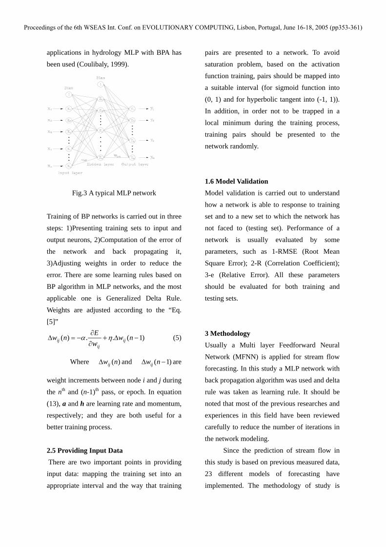
applications in hydrology MLP with BPA has been used (Coulibaly, 1999).

Fig.3 A typical MLP network

Training of BP networks is carried out in three steps: 1)Presenting training sets to input and output neurons, 2)Computation of the error of the network and back propagating it, 3)Adjusting weights in order to reduce the error. There are some learning rules based on BP algorithm in MLP networks, and the most applicable one is Generalized Delta Rule. Weights are adjusted according to the “Eq. [5]”

)1(.)( . −∆∂∂

−=∆ + nwE

nw ijij

ij wηα (5)

Where )(nwij∆ and )1( −∆ nwij are

weight increments between node i and j during the nth and (n-1)th pass, or epoch. In equation

(13), a and h are learning rate and momentum, respectively; and they are both useful for a better training process.

2.5 Providing Input Data There are two important points in providing input data: mapping the training set into an appropriate interval and the way that training

pairs are presented to a network. To avoid saturation problem, based on the activation function training, pairs should be mapped into a suitable interval (for sigmoid function into (0, 1) and for hyperbolic tangent into (-1, 1)). In addition, in order not to be trapped in a local minimum during the training process, training pairs should be presented to the network randomly.

1.6 Model Validation Model validation is carried out to understand how a network is able to response to training set and to a new set to which the network has not faced to (testing set). Performance of a network is usually evaluated by some parameters, such as 1-RMSE (Root Mean Square Error); 2-R (Correlation Coefficient); 3-e (Relative Error). All these parameters should be evaluated for both training and testing sets.

3 Methodology Usually a Multi layer Feedforward Neural Network (MFNN) is applied for stream flow forecasting. In this study a MLP network with back propagation algorithm was used and delta rule was taken as learning rule. It should be noted that most of the previous researches and experiences in this field have been reviewed carefully to reduce the number of iterations in the network modeling.

Since the prediction of stream flow in this study is based on previous measured data, 23 different models of forecasting have implemented. The methodology of study is


based on choosing 2 different categories of models that have two types of input data: single and cumulative form.

In single form, the next month’s flow is considered as a function of single previous month within a year. In this type of modeling, each model has one layer of input data (flow in (t-i)th previous month in which i is between 1, 12) and also one layer as an output data (flow in tth month). According to the value of i

[ 121 ≤≤ i ], 12 networks is developed and for each network, the best combination of hidden layers and the number of neurons are selected.

In cumulative form, flow in the next month is considered as a multi variable function of flow in the previous months. It means, in the first case, flow is considered as the function of flow in previous month and in the last case flow will be forecasted by all 12 months ago.

“Eq. [6], [7]” shows the form of models:

)1(()(1 −=− tQftQ ))2(),1(()(2 −−=− tQtQftQ

.

. ))12(),...,2(),1(()(12 −−−=− tQtQtQftQ

(6) ))1(()(1 −=− tQftQ ))2(()(2 −=− tQftQ

.

. ))12(()(12 −=− tQftQ (7)

In each 23 developed models, (the first

one is same in both cases), the ANN model is trained and tested for available data. Then the selected model, which is either one of the

developed models or a combination of them, will be obtained.

4 Case Study: The Karoon 5 Dam and Power plant Karoon River is the largest surface water resources of Iran. For the moment, the dams Karoon 1 and Masjed Soleiman have been constructed on this river and the dams Upper Gotvand, Karoon3 and Karoon 4 are under construction. The dams Khersan , Bazoft and Karoon 5 at upstream parts of the river are also under study. At the upstream of these sites, Koohrang tunnels of 1 and 2 transfer part of the river water to the neighboring catchments. ”Figure 4” shows the location of region under study.

Inter-basin transfer

Karoon-5 dam site

Great Karoon River Basin

Fig.4 General Layout of study area


The area of river basin at the dam location is 10186 Km2 and the long-term average yield in natural situation (without diversion of water at the upstream parts) is about 114 m3/s Long term average annual precipitation of the watershed is about 613mm. 35m3/s of the river yield is consumed at the upstream or is transferred to the other basins in the neighborhood. Consequently, the annual average inflow to the reservoir is about 78 m3/s. In this study a 43 year time series of inflow (from 1956 to 1998) has been used.

Based on the previous studies (Moshanir 2001), the power plant installed capacity, for plant factor of 25% and normal

water level of 1200 masl with a dam height of 176m (from the river bed at the dam site), has been determines 336 MW .Other required data also prepared based on those studies. While this dam is a hydroelectric production dam, thus only the part of loss function related to this purpose is taken into account. However, the procedure would not be different and generality of the study is not lost.

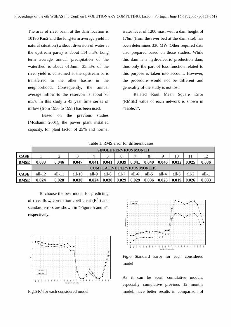
Related Rout Mean Square Error (RMSE) value of each network is shown in “Table.1”.

Table 1. RMS error for different cases

SINGLE PERVIOUS MONTH CASE 1 2 3 4 5 6 7 8 9 10 11 12 RMSE 0.033 0.046 0.047 0.041 0.041 0.039 0.041 0.040 0.040 0.032 0.025 0.036

CUMULATIVE PERVIOUS MONTHS CASE all-12 all-11 all-10 all-9 all-8 all-7 all-6 all-5 all-4 all-3 all-2 all-1 RMSE 0.024 0.028 0.030 0.024 0.030 0.029 0.029 0.036 0.023 0.019 0.026 0.033

To choose the best model for predicting

of river flow, correlation coefficient (R2 ) and standard errors are shown in “Figure 5 and 6”, respectively.

0

0.1

0.2

0.3

0.4

0.5

0.6

0.7

all-1

2

all-1

1

all-1

0

all-9

all-8

all-7

all-6

all-5

all-4

all-3

all-2

all-1 1s

t

2nd

3rd

4th

5th

6th

7th

8th

9th

10th

11th

12th

Case(Previous Months)

R2

Train

Test

Fig.5 R2 for each considered model

100

105

110

115

120

125

130

135

140

145

150

155

160

165

170

175

180

185

190

195

200

all-1

2

all-1

1

all-1

0

all-9

all-8

all-7

all-6

all-5

all-4

all-3

all-2

all-1 1s

t

2nd

3rd

4th

5th

6th

7th

8th

9th

10th

11th

12th

Case(Pervious Months)

Stan

dard

Err

or

TrainTest

Fig.6 Standard Error for each considered model

As it can be seen, cumulative models, especially cumulative previous 12 months model, have better results in comparison of


single models. And the difference between different models in this group is not considerable.

In single models there is a considerable difference between cases. As it can be seen,

value of 2R in 1st, 6th, 11th and 12th month is better than the others.

Consequently, in the first sight, The 12 months cumulative model is the best among them. But this model has the most variables and parameters, which is opposite of parsimony principle while it does not have any mark ably difference in the results with the others. On the other hand, selecting the single input model, there is probability that effect of other months’ in flow will be eliminated. So the conservative approach has been

considered. In which a combination of some past months has been selected instead of considering all 12 months ago. In order to this aim 3 different types of models have been developed. These 3 models are shown in “Eq. [8]”.

))12(),11(),6(),2(),1(()(1 −−−−−=− tQtQtQtQtQftQ

))12(),6(),1(()(2 −−−=− tQtQtQftQ ))12(),1(()(3 −−=− tQtQftQ (8)

The results show that models, which

consist of predicting according to the amount of flow in 1st, 6th and 12th previous month, have the best answer between other cases. “Table 2” shows these results.

Table 2. New combinational models results

Train Data Test Data RMSE R2 Standard

Error R2 Standard Error

Pervious 1st,2nd,6th,11th,12th month 0.02 0.61 105.66 0.60 121.27 Previous 1st, 6th and 12th month 0.02 0.60 107.46 0.62 118.68

Previous 1st and 12th month 0.02 0.56 112.91 0.55 128.71

Comparison of output data (forecasted) and input data (observed) for train and test data are shown in “Figure 7 and 8”, respectively. As it can be seen, the model can successfully predict the amount of flow based on previous months’ data.

0

200

400

600

800

1000

1200

0 25 50 75 100 125 150 175 200 225 250 275 300 325 350 375 400

Month

Flow

(MC

M)

ObservedForecasted

Fig.7 Observed and forecasted flow for train data in selected data


0

100

200

300

400

500

600

700

800

900

1000

0 12 24 36 48 60 72 84 96

Month

Flow

(MC

M)

ObservedForecasted

Fig.8 Observed and forecasted flow for test data in selected data

The applicability of selected model in other combination of train and test data for other cases has been considered. In which 10 and 20 years of data have been applied for training the networks, respectively. However, in each case the remained data has been used in testing process. The R2 and SE has presented in “Table. 3”.

Table3. R2 and Standard Error for 3 form of choosing data

Train Data Test Data

RMSE

R2 Standard

Error R2 Standard

Error all 12 pervious months 0.0308 0.58 78.76 0.57 138.34 10 years as

train data 1th, 6th and 12th pervious month 0.0215 0.51 85.04 0.54 137.55 all 12 pervious months 0.0391 0.54 119.57 0.55 136.90 20 years as

train data 1th, 6th and 12th pervious month 0.0314 0.50 124.49 0.52 133.67 all 12 pervious months 0.0239 0.61 105.66 0.60 121.27 30 years as

train data 1th, 6th and 12th pervious month 0.0205 0.60 107.46 0.62 118.68

Comparison of the correlation coefficient and standard error in predicting of all 12 previous months and 1st, 2nd and 6th past month verify applicability of selected model.

5 CONCLUSION In this study, the ability of ANN in forecasting of river flow was tested and following results have been derived: 1- Forecasting of flow according to cumulative models shows the better results in comparison with single models; however, the input data are too much in these models. 2- Between single models, predicting based on 1st and 12th previous month is reliable, however in this study we used sixth previous month in considered as an effective parameter. 3- According to the results of single models

and choosing the best combination of single input series, a sufficient cumulative model with minimum input data has implemented. 4- In this study, river flow forecasting has conducted only by previous months’ data. Furthermore, better prediction would be derived employing the rainfall, snow and temperature records in the input data, though the selected presented model shows promising results.

Reference: [1] ASCE Task Committee on Application of

Artificial Neural Networks in Hydrology (2000), "Artificial Neural Networks in Hydrology", Journal of Hydrologic Engineering, parts I and II ASCE, 5(2), pp. 115-137.


[2] Coulibaly, P., Anctil F., and Bobee, B. (2001), "Multivariate Reservoir Inflow Forecasting Using Temporal Neural Networks", Journal of Hydrologic Engineering, ASCE, pp. 367-376.

[3] Coulibaly, P., Anctil, F., and Bobee,B.(2000), "Daily reservoir inflow forecasting using artificial neural networks with stopped training approach", J.Hydro., pp. 244-257.

[4] Deo M.C. and Thirumalaiah, K. (2000), "Real Time Forecasting Using Neural Networks" , Artificial Neural Networks in Hydrology , Kluwer Academic Publishing.

[5] Flood, I., Kartam,N., Garret,J.H. (1997), "Artificial Neural Network for civil Engineers: Foundamentals and Applications", ASCE.

[6] Flood, I., Kartam,N. (1998), " Artificial Neural Network for civil Engineers : Advanced Features and Aplications", ASCE .

[7] Garret,J.H., et al. (1993) "Engineering applications of artificial neural networks", J.Intel. Manuf., 4, 1-21.

[8] Jain, S. K., Das , D., and Srivastava, D.K.(1999), "Application of ANN for reservoir inflow prediction and operation", J. Water Resour. Res., 31(10), 2517-2530.

[9] Maidment, David R., (1992). Handbook of Hydrology, McGraw-Hill.

[10] Raman,H., and Sunilkumar,N.(1995), "Multi-variant modeling of water resources time series using artificial neural networks", Hydrological Sci., 40,145-163.

[11] Salas, J.D., Markus, M. and Takar, A.S. (2000), "Streamflow Forecasting based on Artificial Neural Networks", Artificial Neural Networks in Hydrology, Kluwer Academic Publishing.

[12] Sun,C., Neale,C.M.U. , and McDonnel, J.J.(1993), "The potential of using ANN in estimation of snow water equivalent from SSM/I data", Proc., Engrg. Hydrol., ASCE, New York.

[13] Thirumalaiah, K., and Deo, M. C. (2000), "Hydrological Forecasting Using Neural Networks", Journal of Hydrologic Engineering, ASCE, 5(2), pp. 180-189.

[14] Tokar, S., and Markus, M.,(2000), "Precipitation-Runoff Modeling Using Artificial Neural Networks and Conceptual Models", Journal of Hydrologic Engineering, ASCE, 3(1), pp. 156-161.


River Flow Forecasting with ANN

Documents

Transcript of River Flow Forecasting with ANN