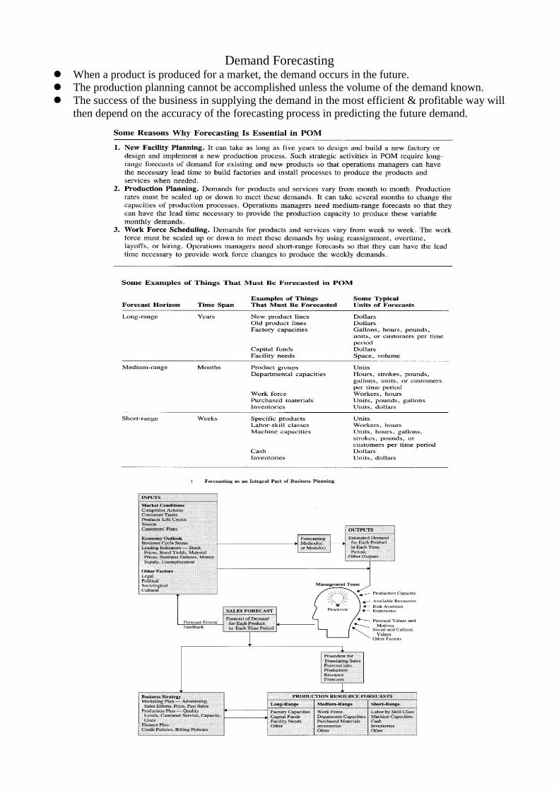
Demand Forecasting When a product is produced for a market, the demand occurs in the future. The production planning cannot be accomplished unless the volume of the demand known. The success of the business in supplying the demand in the most efficient & profitable way will

then depend on the accuracy of the forecasting process in predicting the future demand.

Technique for Demand Forecasting1. Naïve techniques - adding a certain percentage to the demand for next year.2. Opinion sampling - collecting opinions from sales, customers etc.3. Qualitative methods4. Quantitative methods - based on statistical and mathematical concepts.

a. Time series - the variable to be forecast has behaved according to a specific pattern in thepast and that this pattern will continue in the future.

b. Causal - there is a causal relationship between the variable to be forecast and anothervariable or a series of variables.

Quantitative Methods of Forecasting1.Causal–There is a causal relationship between the variable to be forecast and another variable

or a series of variables. (Demand is based on the policy, e.g. cement, and build material.2.Time series–The variable to be forecast has behaved according to a specific pattern in the past

and that this pattern will continue in the future.

Causal:Demand for next period= f (number of permits, number of loan application....)

Time series:1. D = F (t)Where D is the variable to be forecast and f(t) is a function whose exact form can be estimatedfrom the past data available on the variable.2. The value of the variable for the future as a function of its values in the past.Dt+1 = f ( Dt, Dt-1, Dt-2, .....) There exists a function whose form must be estimated using the available data.. The most common technique for estimation of equation is regression analysis.

Regression Analysis: is not limited to locating the straight line of best fit.

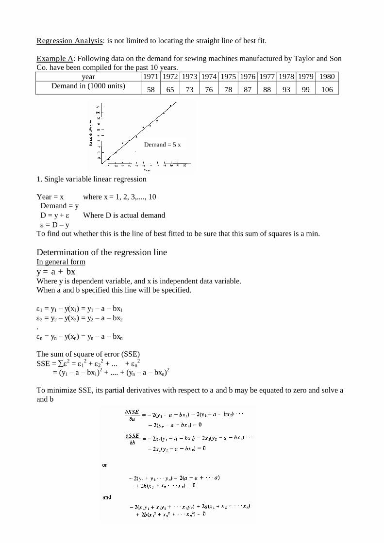
Example A: Following data on the demand for sewing machines manufactured by Taylor and SonCo. have been compiled for the past 10 years.

year 1971 1972 1973 1974 1975 1976 1977 1978 1979 1980Demand in (1000 units) 58 65 73 76 78 87 88 93 99 106

1. Single variable linear regression

Year = x where x = 1, 2, 3,...., 10Demand = yD = y + Where D is actual demand= D–y

To find out whether this is the line of best fitted to be sure that this sum of squares is a min.

Determination of the regression lineIn general formy = a + bxWhere y is dependent variable, and x is independent data variable.When a and b specified this line will be specified.

1 = y1–y(x1) = y1–a–bx1

2 = y2–y(x2) = y2–a–bx2

.n = yn–y(xn) = yn–a–bxn

The sum of square of error (SSE)SSE = 2 = 1

2 + 22 + ... + n

2

= (y1–a–bx1)2 + .... + (yn–a–bxn)2

To minimize SSE, its partial derivatives with respect to a and b may be equated to zero and solve aand b

Demand = 5 x

Coefficient of correlation

Where -1 r 1*Perfect interdependence between variables when 1

2. Exponential: sometimes a smooth curve provides a better fit for data points than does a straightline y = abx indicates that y changes in each period at the constant rate b.

Determine the value for a and b by the least squares method:log y = log a + x log b

The logarithmic version plots as a straight line on semi-logarithmic paper: the Y scale is logarithmicand the X scale arithmetic.

bXaXYX

bXaNY

logloglog

logloglog2

2

loglog

loglog

X

YXb

andN

Ya

- If the curved line from the exponential equation does not represent the data adequately,forecasting equation can be based on algebraic series such as,Y = a +b1X + b2X2 + … + bnXn

- Or trigonometric functions such asY = a + b1sin(2X/b2) + b3 cos(2X/b4)

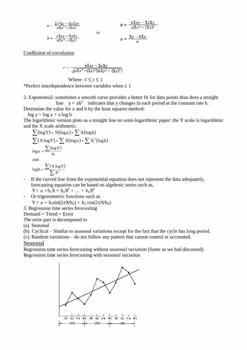
3. Regression time series forecastingDemand = Trend + ErrorThe error part is decomposed to(a). Seasonal(b). Cyclical–Similar to seasonal variations except for the fact that the cycle has long period.(c). Random variations–do not follow any pattern that cannot control or accounted.SeasonalRegression time series forecasting without seasonal variation (Same as we had discussed)Regression time series forecasting with seasonal variation

or

Example: Demand for sporting goods for sports, golf, swimming Different types of clothing, food, and heating and cooling systems

Example B: The demand for a certain soft drink in the past four years in given in following on aquarterly basis.

Year Period Demand(in Million)

Year Period Demand(in Million)

1 Spring 15 3 Spring 20Summer 25 Summer 30

Fall 16 Fall 18Winter 8 Winter 11

2 Spring 17 4 Spring 18Summer 29 Summer 32

Fall 14 Fall 19Winter 10 Winter 12

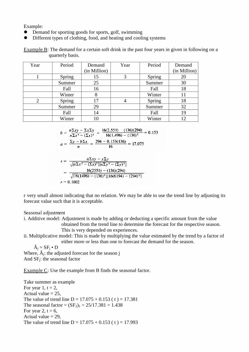
r very small almost indicating that no relation. We may be able to use the trend line by adjusting itsforecast value such that it is acceptable.

Seasonal adjustmenti. Additive model: Adjustment is made by adding or deducting a specific amount from the value

obtained from the trend line to determine the forecast for the respective season.This is very depended on experiences.

ii. Multiplicative model: This is made by multiplying the value estimated by the trend by a factor ofeither more or less than one to forecast the demand for the season.

Ãj = SFj • DWhere, Ãj: the adjusted forecast for the season jAnd SFj: the seasonal factor

Example C: Use the example from B finds the seasonal factor.

Take summer as exampleFor year 1, t = 2,Actual value = 25,The value of trend line D = 17.075 + 0.153 ( t ) = 17.381The seasonal factor = (SF2)1 = 25/17.381 = 1.438For year 2, t = 6,Actual value = 29,The value of trend line D = 17.075 + 0.153 ( t ) = 17.993

The seasonal factor = (SF2)2 = 25/17.993 = 1.612

For year 3, t = 10,Actual value = 30,The value of trend line D = 17.075 + 0.153 ( t ) = 18.605The seasonal factor = (SF2)3 = 25/18.605 = 1.612

For year 4, t = 14,Actual value = 32,The value of trend line D = 17.075 + 0.153 ( t ) = 19.217The seasonal factor = (SF2)4 = 25/19.217 = 1.665

Average these four values yield the seasonal adjustment factor for the summer season of any year.

SF2 = [(SF2)1 + (SF2)2 + (SF2)3 + (SF2)4]/4 = 1.582

Now to find the forecast for the summer of year 5, i.e. t = 18D = 17.075 + 0.153 ( t ) = 19.829Ãj = SFj • D = 1.582 • 19.829 = 31.369

With the same techniques we may findSpring SF2 = 0.963Fall SF2 = 0.906Winter SF2 = 0.549

Forecasting by Time Series Analysis(short-range forecast) - Without using regressionanalysis

These models are especially helpful when there is no clear upward or downward pattern in the pastdata to suggest a kind of linear relationship between the demand and time.In general

Dt+1 = F (Dt, Dt-1, ...., D2, D1)Where Dt+1 is forecast demand for the next period

(a). Simple moving average forecasting(b). Exponential smoothing

Simple moving average forecasting All past data are given equal weight in estimating.

Dt+1 =1/k •(Dt, + Dt-1 + ....+ D2 + D1)

Example C. Simple Moving Average ForecastingThe demand for the past 12 years of certain type of automobile alternator is given belowyear Demand year Demand

(in 10,000 units) (in 10,000 units)69 32 75 4070 40 76 2571 50 77 5272 28 78 4873 30 79 4074 44 80 44

A. Three period moving average forecast for the demandDt+1 =1/3 • (Dt, + Dt-1 + Dt-2)

B. Five period moving average is given byDt+1 =1/5 •((Dt, + Dt-1 + Dt-2 + Dt-3 + Dt-4)

For example:D81 =1/3 • (D80, + D79 + D78) = 44

D81 =1/5 • (D80, + D79 + D78+ D77+ D76) = 41.8

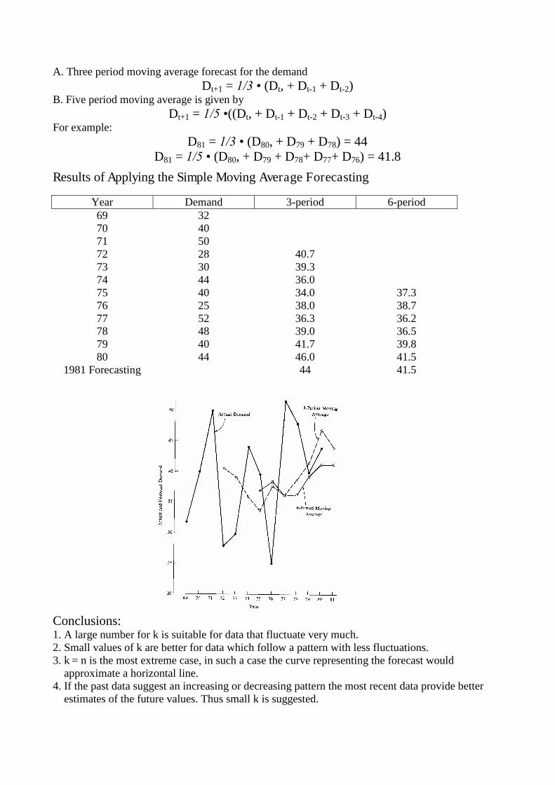
Results of Applying the Simple Moving Average Forecasting

Year Demand 3-period 6-period69 3270 4071 5072 28 40.773 30 39.374 44 36.075 40 34.0 37.376 25 38.0 38.777 52 36.3 36.278 48 39.0 36.579 40 41.7 39.880 44 46.0 41.5

1981 Forecasting 44 41.5

Conclusions:1. A large number for k is suitable for data that fluctuate very much.2. Small values of k are better for data which follow a pattern with less fluctuations.3. k = n is the most extreme case, in such a case the curve representing the forecast would

approximate a horizontal line.4. If the past data suggest an increasing or decreasing pattern the most recent data provide better

estimates of the future values. Thus small k is suggested.

Weighted Moving Average Method In some situations, it may be desirable to apply unequal weights to the historical data

Actual Weight72 28 .2073 30 .3074 44 .50

Modification of Forecast75=36.6

Exponential smoothing Exponential smoothing is assumed that the future demand is the same as the forecast made for

the present period plus a percentage of the forecasting error made in the past period.Ft+1 = Ft + ( Dt–Ft )Where is smoothing factorExample D. Exponential SmoothingA new product demand for January and February of this year has been 40,000 and 48,000respectively. New product has no additional information. Forecast the demand for March with =0.4.Solution:FM = FF + ( DF–FF )FF = FJ + ( DJ–FJ )FJ is unknown, since no additional information is available, we assumeFJ = DJ = 40,000 and FF = FJ = 40,000 FM = 4,000 + 0.4 (48,000–40,000) = 43,200 More detail about exponential smoothing (if we know more past).

Ft+1 = Ft + ( Dt–Ft )Expand the equationFt+1 = Dt + (1- ) Ft

Substitute Ft with Ft+1

Ft+1 = Dt-1 + (1- ) Ft-1

Ft+1 = Dt + (1- ) Dt-1 + (1- )2 Ft-1

With the same procedure on Ft-1 and Ft-2The general form can be written asFt+1 = Dt + (1- ) Dt-1 + (1- )2 Dt-2 + ....+ (1- )t-1 D1 + (1- )t F1

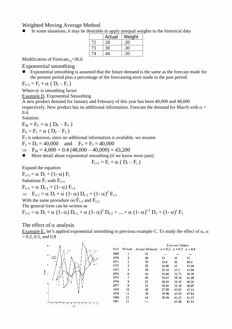
The effect of analysisExample E. let’s applied exponential smoothing to previous example C. To study the effect of , = 0.2, 0.5, and 0.8

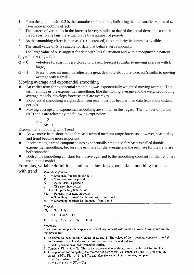
1. From the graphic with 0.2 is the smoothest of the three, indicating that the smaller values of have more smoothing effect.

2. The pattern of variations in the forecast in very similar to that of the actual demand except thatthe forecast curve lags the actual curve by a number of periods.

3. As the smoothing effect is increased (decreased) this similarity becomes less visible.4. The small value of is suitable for data that behave very randomly.5. The large value of is suggest for data with less fluctuation and with a recognizable pattern.Ft+1 = Ft + ( Dt –Ft )0 Future forecast in very closed to present forecast (Similar to moving average with k

large)1 Present forecast much be adjusted a great deal to yield future forecast (similar to moving

average with k small)Moving average and exponential smoothing An earlier term for exponential smoothing was exponentially weighted moving average. This

term reminds us the exponential smoothing, like the moving average and the weighted movingaverage models, develops forecasts that are averages.

Exponential smoothing weights data from recent periods heavier than data from more distantperiods

Moving average and exponential smoothing are similar in this regard. The number of period(AP) and a are related by the following expression:

Exponential Smoothing with Trend As we move from short-range forecasts toward medium-range forecasts, however, seasonality

and trend become more important. Incorporating a trend component into exponentially smoothed forecasts is called double

exponential smoothing, because the estimate for the average and the estimate for the trend areboth smoothed.

Both a, the smoothing constant for the average, and b, the smoothing constant for the trend, areused in this model.

Formulas, variable definitions, and procedure for exponential smoothing forecastswith trend

12

AP

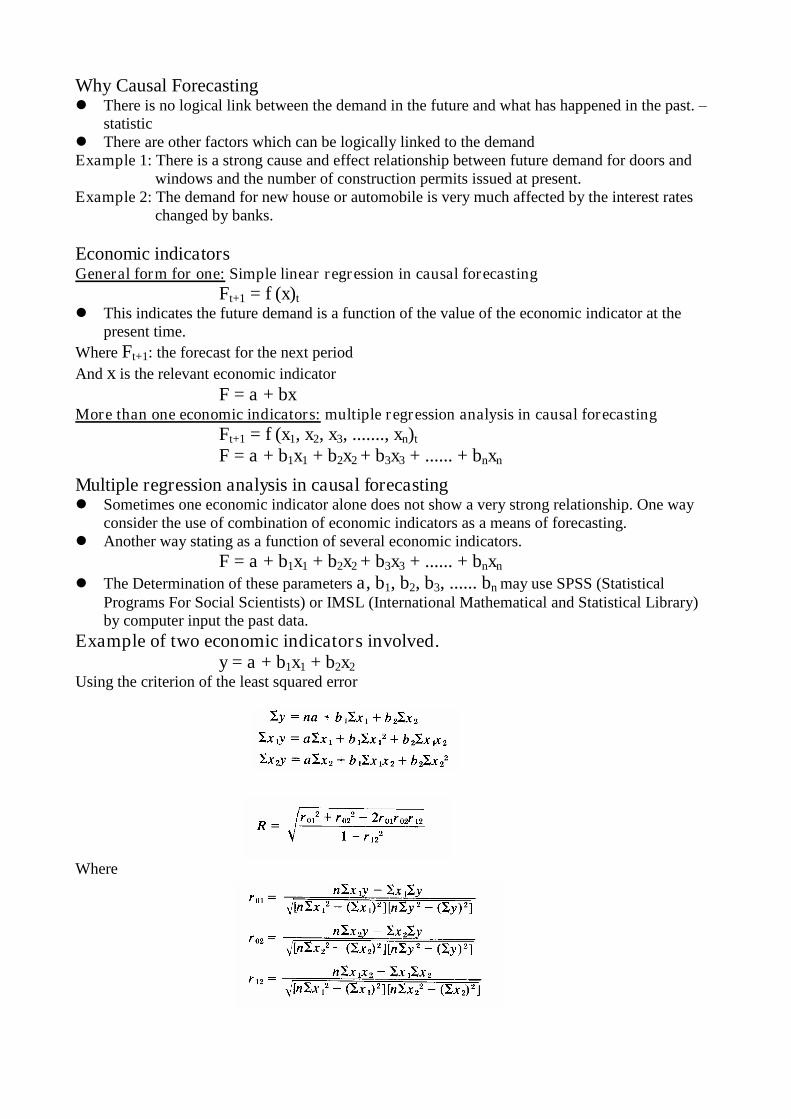
Why Causal Forecasting There is no logical link between the demand in the future and what has happened in the past.–

statistic There are other factors which can be logically linked to the demandExample 1: There is a strong cause and effect relationship between future demand for doors and

windows and the number of construction permits issued at present.Example 2: The demand for new house or automobile is very much affected by the interest rates

changed by banks.

Economic indicatorsGeneral form for one: Simple linear regression in causal forecasting

Ft+1 = f (x)t This indicates the future demand is a function of the value of the economic indicator at the

present time.Where Ft+1: the forecast for the next periodAnd x is the relevant economic indicator

F = a + bxMore than one economic indicators: multiple regression analysis in causal forecasting

Ft+1 = f (x1, x2, x3, ......., xn)t

F = a + b1x1 + b2x2 + b3x3 + ...... + bnxn

Multiple regression analysis in causal forecasting Sometimes one economic indicator alone does not show a very strong relationship. One way

consider the use of combination of economic indicators as a means of forecasting. Another way stating as a function of several economic indicators.

F = a + b1x1 + b2x2 + b3x3 + ...... + bnxn

The Determination of these parameters a, b1, b2, b3, ...... bn may use SPSS (StatisticalPrograms For Social Scientists) or IMSL (International Mathematical and Statistical Library)by computer input the past data.

Example of two economic indicators involved.y = a + b1x1 + b2x2

Using the criterion of the least squared error

Where

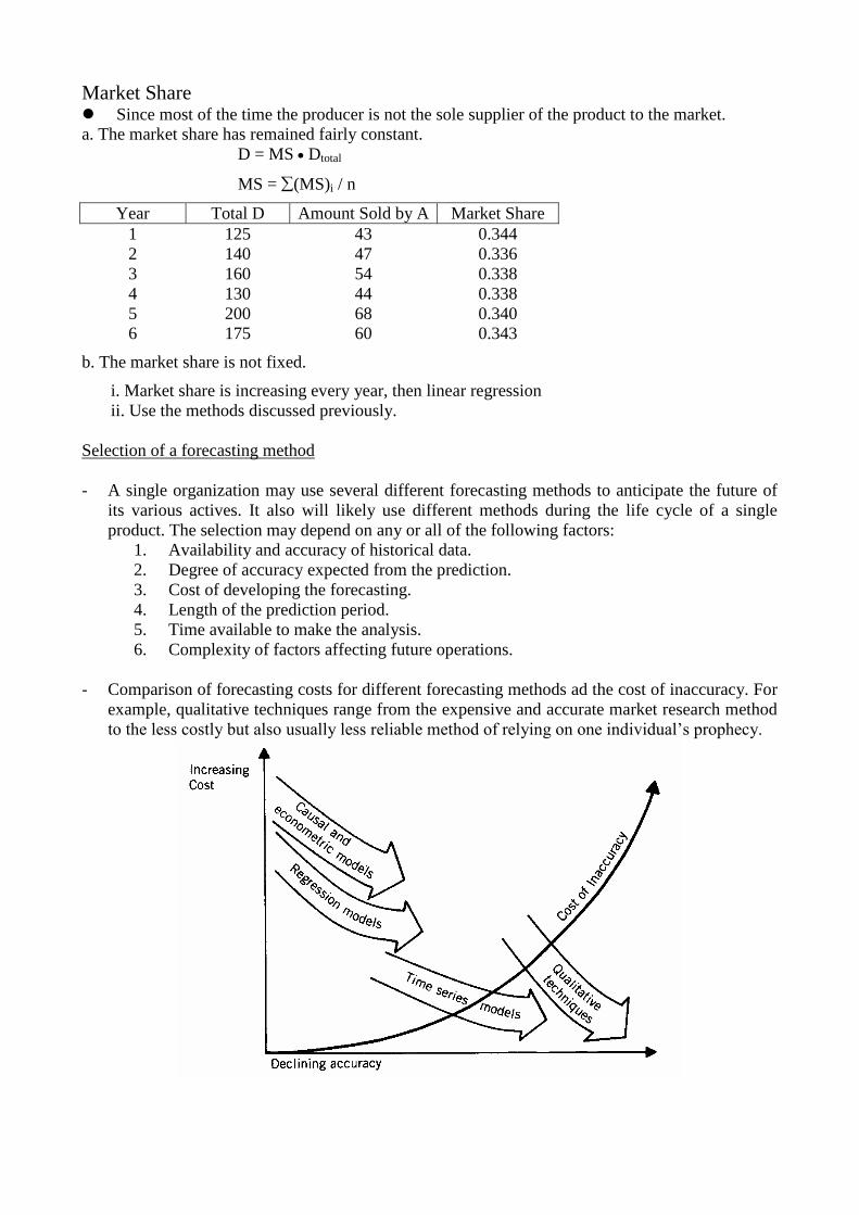
Market Share Since most of the time the producer is not the sole supplier of the product to the market.a. The market share has remained fairly constant.

D = MS Dtotal

MS = (MS)i / n

Year Total D Amount Sold by A Market Share1 125 43 0.3442 140 47 0.3363 160 54 0.3384 130 44 0.3385 200 68 0.3406 175 60 0.343

b. The market share is not fixed.

i. Market share is increasing every year, then linear regressionii. Use the methods discussed previously.

Selection of a forecasting method

- A single organization may use several different forecasting methods to anticipate the future ofits various actives. It also will likely use different methods during the life cycle of a singleproduct. The selection may depend on any or all of the following factors:

1. Availability and accuracy of historical data.2. Degree of accuracy expected from the prediction.3. Cost of developing the forecasting.4. Length of the prediction period.5. Time available to make the analysis.6. Complexity of factors affecting future operations.

- Comparison of forecasting costs for different forecasting methods ad the cost of inaccuracy. Forexample, qualitative techniques range from the expensive and accurate market research methodto the less costly but also usually less reliable method of relying on one individual’s prophecy.

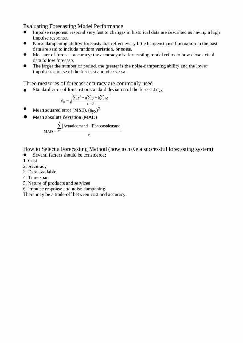
Evaluating Forecasting Model Performance Impulse response: respond very fast to changes in historical data are described as having a high

impulse response. Noise dampening ability: forecasts that reflect every little happenstance fluctuation in the past

data are said to include random variation, or noise. Measure of forecast accuracy: the accuracy of a forecasting model refers to how close actual

data follow forecasts The larger the number of period, the greater is the noise-dampening ability and the lower

impulse response of the forecast and vice versa.

Three measures of forecast accuracy are commonly used Standard error of forecast or standard deviation of the forecast syx

Mean squared error (MSE), (syx)2

Mean absolute deviation (MAD)

How to Select a Forecasting Method (how to have a successful forecasting system) Several factors should be considered:1. Cost2. Accuracy3. Data available4. Time span5. Nature of products and services6. Impulse response and noise dampeningThere may be a trade-off between cost and accuracy.

2

2

n

xybyayS yx

n

mandForecastdendActualdemaMAD

n

i

1