Forecasting Demand for Optimal Inventory with Long Lead ...
97
University of Missouri, St. Louis University of Missouri, St. Louis IRL @ UMSL IRL @ UMSL Dissertations UMSL Graduate Works 11-12-2021 Forecasting Demand for Optimal Inventory with Long Lead Times: Forecasting Demand for Optimal Inventory with Long Lead Times: An Automotive Aftermarket Case Study An Automotive Aftermarket Case Study Chris Anderson University of Missouri-St. Louis, [email protected] Follow this and additional works at: https://irl.umsl.edu/dissertation Part of the Business Analytics Commons, Management Sciences and Quantitative Methods Commons, and the Operations and Supply Chain Management Commons Recommended Citation Recommended Citation Anderson, Chris, "Forecasting Demand for Optimal Inventory with Long Lead Times: An Automotive Aftermarket Case Study" (2021). Dissertations. 1105. https://irl.umsl.edu/dissertation/1105 This Dissertation is brought to you for free and open access by the UMSL Graduate Works at IRL @ UMSL. It has been accepted for inclusion in Dissertations by an authorized administrator of IRL @ UMSL. For more information, please contact [email protected].
-
Upload
khangminh22 -
Category
Documents
-
view
2 -
download
0
Transcript of Forecasting Demand for Optimal Inventory with Long Lead ...

University of Missouri, St. Louis University of Missouri, St. Louis
IRL @ UMSL IRL @ UMSL
Dissertations UMSL Graduate Works
11-12-2021
Forecasting Demand for Optimal Inventory with Long Lead Times: Forecasting Demand for Optimal Inventory with Long Lead Times:
An Automotive Aftermarket Case Study An Automotive Aftermarket Case Study
Chris Anderson University of Missouri-St. Louis, [email protected]
Follow this and additional works at: https://irl.umsl.edu/dissertation
Part of the Business Analytics Commons, Management Sciences and Quantitative Methods
Commons, and the Operations and Supply Chain Management Commons
Recommended Citation Recommended Citation Anderson, Chris, "Forecasting Demand for Optimal Inventory with Long Lead Times: An Automotive Aftermarket Case Study" (2021). Dissertations. 1105. https://irl.umsl.edu/dissertation/1105
This Dissertation is brought to you for free and open access by the UMSL Graduate Works at IRL @ UMSL. It has been accepted for inclusion in Dissertations by an authorized administrator of IRL @ UMSL. For more information, please contact [email protected].

Copyright, Christopher J. Anderson, 2021
Forecasting Demand for Optimal Inventory with Long Lead Times:
An Automotive Aftermarket Case Study
Christopher J. Anderson
Master of Business Administration – Pepperdine University, 1990
B.S. Electrical Engineering – Southern Illinois University, 1984
A Dissertation Submitted to The Graduate School at the University of Missouri–St. Louis
in partial fulfillment of the requirements for the degree
Doctor of Business Administration with an Emphasis in Operations Management
December 2021
Advisory Committee
Keith Womer, Ph.D.
Chairperson
George A. Zsidisin, Ph.D.
Hung-Gay Fung, Ph.D.

Forecasting Demand with Long Lead Times 2
Copyright, Christopher J. Anderson, 2021
Abstract
Accuracy in predicting customer demand is essential to building an economic
inventory policy under periodic review, long lead-time, and a target fill rate. This study
uses inventory and customer service level as a stock control metric to evaluate the
forecast accuracy of different simple to more complex predictive analytical techniques.
We show how traditional forecast error measures are inappropriate for inventory control,
despite their consistent usage in many studies, by evaluating demand forecast
performance dynamically with customer service level as a stock control metric that
includes inventory holdings costs, stock out costs, and fill rate service levels. A second
contribution includes evaluating the utility of introducing more complexity into the
forecasting process for an automotive aftermarket parts manufacturer and the superior
inventory control results using the Prais-Winsten, an econometric method, for non-
intermittent demand forecasting with long-lead times. This study will add to the limited
case study research on demand forecasting under long lead times using stock control
metrics, dynamic model updating, and the Prais-Winsten method for inventory control.
Keywords: inventory control, Prais-Winsten, automotive parts, customer service
level, stock control, rolling origin cross-validation, dynamic model updating.

Forecasting Demand with Long Lead Times 3
Copyright, Christopher J. Anderson, 2021
Acknowledgments
There have been numerous people who have aided me on this journey. I want to
express my gratitude to them. First and foremost, I want to express my sincere thanks to
my dissertation committee and group. I would not have made it if it hadn't been for their
invaluable counsel and assistance. Dr. George Zsidisin, Dr. Hung-gay Fung, Dr. Doug
Smith, and my Chair, Dr. Keith Womer, went above and above to assist me in achieving
my objective. To my friends who have endured me being preoccupied and skipping
several gatherings. For your patience and understanding, I am eternally thankful. I'm
hoping to reconnect with every one of you now that I have some more free time. To my
dog Clark, who kept me company as I coded in R, tested, analyzed, wrote, and revised
the final result. Finally, I want to thank my wife, Julie, and my daughter, Stephanie, for
their love and understanding through these trying times. I would not have succeeded if
you had not believed in me. It's time to rejoice; you received this degree alongside me.

Forecasting Demand with Long Lead Times 4
Copyright, Christopher J. Anderson, 2021
Table of Contents
Abstract .................................................................................................................. 2
Acknowledgments ................................................................................................. 3
Chapter 1: Introduction ....................................................................................... 8
Analytics .............................................................................................................. 9
Predictive Analytics Assimilation ..................................................................... 11
Optimal Inventory ............................................................................................. 14
Case: Automotive Aftermarket Manufacturer ................................................... 14
Chapter 2: Literature Review ............................................................................ 19
Forecasting Methods ......................................................................................... 22
Intermittent Data ............................................................................................... 26
Exogenous Data ................................................................................................. 27
Evaluation Criteria ............................................................................................ 29
Rolling Origin Cross-Validation .................................................................. 31
Company Adoption ........................................................................................... 32
Chapter 3: Research Methodology .................................................................... 34
Measures ............................................................................................................ 34
Exogenous Variables ......................................................................................... 36
Google Trends Search Data ......................................................................... 37
Methods ............................................................................................................. 39
Procedure ........................................................................................................... 42
Step One – Collect Data............................................................................... 43
Step Two – Prepare Data ............................................................................. 43
Step Three – Analyze Data .......................................................................... 44
Step Four – Forecast Demand ...................................................................... 46
Step Five – Determine Order ....................................................................... 48
Step Six – Evaluate Performance................................................................. 49
Step Seven – Add Exogenous Variable and Repeat .................................... 52
Chapter 4: Results............................................................................................... 55
Single Forecasting Model Results ..................................................................... 55
Multiple Forecasting Model Results ................................................................. 61

Forecasting Demand with Long Lead Times 5
Copyright, Christopher J. Anderson, 2021
Results Summay ................................................................................................ 64
Chapter 5: Discussion ......................................................................................... 66
Limitations ........................................................................................................ 67
Extensions and Future Research ....................................................................... 68
Conclusions ....................................................................................................... 70
References ............................................................................................................ 71
Appendix – R Program Code ............................................................................. 84

Forecasting Demand with Long Lead Times 6
Copyright, Christopher J. Anderson, 2021
List of Figures
Figure 1. Flow of Parts .................................................................................................... 16
Figure 2. SBA Classification ............................................................................................. 27
Figure 3 Rolling Origin with Constant In-Sample Window .............................................. 32
Figure 4. Clutch Part Aggregate Demand ........................................................................ 34
Figure 5. Smooth Parts Sample ......................................................................................... 36
Figure 6. Google Trends for "clutch" ............................................................................... 37
Figure 7. Procedure Steps ................................................................................................. 42
Figure 8. Google Trends Autocorrelation Plot ................................................................. 46
Figure 9. Google Trends Partial Autocorrelation Plot ..................................................... 46
Figure 10. Rolling Origin Cross Validation with Constant In-Sample Window .............. 51
Figure 11. Prais-Winsten Last 13 Month Inventory Cost ................................................. 58
Figure 12. Prais-Winsten Last 13 Month Inventory Cost Excluding the Last 10 Part
Numbers ..................................................................................................................... 59
Figure 13. Part 360098 Sales Demand and Inventory ...................................................... 60
Figure 14. Part Number Models over the Last 13 Month Inventory Cost ........................ 62
Figure 15. Part Number Models Last 13 Month Inventory Cost Excluding 3 Part
Numbers .................................................................................................................... 63

Forecasting Demand with Long Lead Times 7
Copyright, Christopher J. Anderson, 2021
List of Tables
Table 1. Forecasting Methods ............................................................................... 23
Table 2. Exogenous Automotive Research ........................................................... 27
Table 3. SBA Classification .................................................................................. 35
Table 4. R Model Calls ......................................................................................... 47
Table 5. R Xreg Model Calls ................................................................................ 53
Table 6. Average Forecasting Model Performance .............................................. 56
Table 7. Average Forecast Model Performance in the Last 13 Months ............... 57
Table 8. Select Forecasting Model Performance .................................................. 62

Forecasting Demand with Long Lead Times 8
Copyright, Christopher J. Anderson, 2021
Chapter 1: Introduction
Many businesses that carry inventory either have too much of it, which is
expensive, or too little, leading to stockouts and lost sales. Inventory constitutes the most
significant portion of current assets for most manufacturing firms tying up significant
organizational capital (Singh & Verma, 2018). An essential factor in firms achieving
optimal inventory is demand forecasting (Kocer, 2013), part of the sales and operational
planning process. Managers need to identify suitable sources of external data and simple
analytical tools that are easy to use to reliably gauge the effectiveness of demand
forecasts and draw conclusions on what inventory to order (Blackburn, Lurz, Priese, Göb,
& Darkow, 2015). Long lead times can lead to inaccurate forecasts caused by delays in
replenishment, which is one of the many reasons for poor inventory management (i.e.,
supplier delivery performance, poor material yields, poor supplier quality, inappropriate
order quantities). Accuracy in forecasting demand is crucial to developing a good
inventory policy and managing an effective supply chain. The use of complex forecasting
methods increases the opportunities for errors in judgment, understanding, prediction,
and explanatory power (Green & Armstrong, 2015), so simple analytical methods are
essential for practical use and easier assimilation. Simple forecasting and accurate
demand planning are large factors in appropriately managing optimal inventory.
This study focuses on demand forecasting under long lead times using dynamic
model parameter updating for exponential smoothing (ES), its variants double ES, triple
ES; linear regression, autocorrelation using the Prais-Winsten transformation, and some
more straightforward time series methods naïve and simple moving average (SMA) as we

Forecasting Demand with Long Lead Times 9
Copyright, Christopher J. Anderson, 2021
seek to answer the question: do complex forecasting methods increase forecasting
accuracy? The study will also add exogenous data from Google Trends to answer: Can
exogenous data improve demand forecasting?
The related literature typically addresses optimal inventory and demand
forecasting as separate questions. However, the availability of cost information will
estimate the economic effects of changing forecast parameters on inventory. Finally, the
study will examine the relationship between traditional forecast measures of accuracy,
such as Mean Error (ME), Root Mean Squared Error (RMSE) or Mean Absolute Error
(MAE), and customer service level (CSL) as stock control metric in the calculation of
economic order quantity (EOQ), which consider measures like holdings costs, ordering
costs, and service levels based on fill rate. All to answer the question: how can CSL stock
control metrics be used to evaluate forecast accuracy?
The overall goal is to determine the best use of historical data to make ordering
decisions with long lead times and find a relatively easy to use optimal inventory policy
with periodic review and a target fill rate using CSL stock control metrics for an
automobile aftermarket parts company without introducing too much complexity into the
forecasting process. Moreover, it adds to the limited empirical research on demand
forecasting under long lead times, CSL stock control metrics, and dynamic model
parameter updating. This study will try to answer the question: Can a procedure be
developed that is likely to be adopted?
Analytics
Big data and predictive analytic (BDPA) tools used to improve decision making
and material flow are rapidly evolving within supply chain analytics, growing in response

Forecasting Demand with Long Lead Times 10
Copyright, Christopher J. Anderson, 2021
to the volumes of data made available in the Internet age. The analytical methods used in
supply chain analytics fall into three types: descriptive analytics, predictive analytics, or
prescriptive analytics (Souza, 2014). Descriptive analytics looks at past events up to the
present (real-time) and tries to answer what happened or what is happening. For example,
analyzing radio frequency identification (RFID) location data to understand how material
flowed through the plant to streamline material flow, optimize material handling, or track
inventory. Predictive analytics evaluates the output from descriptive analytics to forecast
or predict the likelihood of what will happen at a future time. For example, predictive
maintenance uses past machine failure data to estimate the likelihood of critical
components failing to schedule machine maintenance cycles.
Prescriptive analytics builds on both the descriptive and predictive analytics
outputs to determine the best course of action or what should happen, or how it can be
made to happen. For example, using data on past deliveries to determine how long it will
take (lead time) for the supplier deliveries, or using past production data to determine the
turnaround time to fill the order, or using both to prescribe the order quantity, given the
variability in demand, supplier lead time, and production lead time. Another example is
using past sales ordering or demand data from previous customers to determine how
much stock was needed (order quantity) to meet the demand to determine the stocking
order for a new customer account. New customers have no previous sales data to
calibrate the stocking order, but there is data on similar customers and their order patterns
to estimate new account ordering. Predictive and prescriptive analytics are very similar.
The difference is that predictive analytics is focused on the outcome, while prescriptive
analytics considers various future situations to prescribe a course of action.

Forecasting Demand with Long Lead Times 11
Copyright, Christopher J. Anderson, 2021
In the last few decades, interest in data science, machine learning, and the use of
big data has exploded, bringing with it a host of new conferences, journals, software
companies, and even prizes for forecasting research (R. Fildes, Nikolopoulos, Crone, &
Syntetos, 2008b). Interest in supply chain analytics has grown alongside data science,
emphasizing predictive analytics for demand forecasting.
Predictive Analytics Assimilation
Supply chain organizations have collected and stored vast amounts of digital data
for years (Dekker, Pinçe, Zuidwijk, & Jalil, 2013). These datasets have enabled the
growth in supply chain management (SCM) data analytics techniques involving data
mining and statistical analysis to develop more accurate predictive analytics to forecast
behavior. The collection and sharing of information along the supply chain result in a
more intelligent supply chain armed with analytical tools and techniques to be more
efficient and allow more data-driven decisions (Govindan, Cheng, Mishra, & Shukla,
2018), and improve profitability. Effectively utilizing vast amounts of historical and real-
time data to improve the organizations' performance and their supply chains are what big
data and predictive analytics (BDPA) promises. Assimilating predictive analytic methods
into the organization is one area of sustaining and disruptive technology research growing
in importance within both academics and practitioners of SCM.
BDPA is used to solve complex supply chain problems and improve overall
business process performance (Wang, Gunasekaran, Ngai, & Papadopoulos, 2016).
Problems like the bullwhip effect, demand forecasting, order flow along the supply chain,
and optimizing flow use analytics to improve business performance. There are many
opportunities inside existing processes using descriptive analytics, forecasting future

Forecasting Demand with Long Lead Times 12
Copyright, Christopher J. Anderson, 2021
demand with predictive analytics, and making better decisions using prescriptive
analytics. Although, companies struggle with assimilating methods with a sufficient
understanding to utilize the forecasts to make better decisions.
BDPA assimilation across the organization and occurs in three phases starting
with acceptance, moving on to a routine, and ending in the assimilation of BDPA (Hazen,
Overstreet, & Cegielski, 2012). The acceptance stage encompasses the growing
awareness of BDPA and how well stakeholders understand the scope of BDPA in their
job. The routine phase begins when the organization's systems of governance are altered
to incorporate BDPA. Furthermore, assimilation occurs when BDPA has spread through
all affected business processes. BDPA assimilation research has found a positive
association with both organizational performance (OP) and supply chain performance
(SCP) (Gunasekaran et al., 2017). Once assimilated, data is parsed into actionable
knowledge items displayed with visual dashboards to identify problems (Bumblauskas,
Nold, Bumblauskas, & Igou, 2017). While some have found data quality or data security
a significant barrier (Verma, Bhattacharyya, & Kumar, 2018), others believe the most
significant barriers to BDPA adoption are learning how to use BDPA to improve
performance (LaValle, Lesser, Shockley, Hopkins, & Kruschwitz, 2011). Some have
suggested a tiered model involving the three primary elements of management,
technology, and human capability (Akter, Wamba, Gunasekaran, Dubey, & Childe,
2016). BDA skills, talent, and management capability are emerging as the strongest
indicator of BDA success, suggesting a well-developed approach to recruiting analytics
talent (Court, 2015) will help achieve a sustainable competitive advantage with BDA. To
assist in overcoming these barriers, Lamba and Singh (2018) found the most significant

Forecasting Demand with Long Lead Times 13
Copyright, Christopher J. Anderson, 2021
driving enablers for big data deployment and use are top management commitment,
financial backing, BDPA skills, organizational BDPA infrastructure, and a change
management program.
There are many positive SCM effects to using BDPA, ranging from increased
supply chain visibility, efficiency, and maintenance to improved integration,
collaboration, and product design (Kache & Seuring, 2017). BDPA has evolved into a
vital strategic component adding a new competitive advantage for those companies that
fully embrace its' assimilation into the organization. Companies that have learned to sift
through substantial amounts of historical supply chain and public data have positioned
themselves to improve decision making and deliver the efficiency and effectiveness they
desire, with lower costs, greater global SCM capabilities, increased BDPA skills, and a
sustainable competitive advantage. Assimilating BDPA technology and methods into the
organization is the key to securing a competitive advantage.
The evaluation process starts with the baseline forecast that the company uses
now compared with various forecasting methods and the additional predictor variables to
determine the new improvement level. The intent is to compare what the automotive parts
manufacturer is currently doing for forecasting to methods for demand forecasting based
on predictive analytics research that combines exogenous data. We will use stochastic
inventory models, stock control, and customer service level metrics to evaluate the
performance of the demand forecasts. This study intends to address uncertain demand
using a prescriptive analytics approach to determine optimal inventory. Although data
from the automotive aftermarket space is the primary focus, the study methods apply to
other companies or markets seeking to solve the uncertain demand problem.

Forecasting Demand with Long Lead Times 14
Copyright, Christopher J. Anderson, 2021
Optimal Inventory
Previous research into optimal inventory policy has focused almost exclusively on
customer demand using various forms of the Economic Order Quantity (EOQ) model to
determine the inventory level (Harris, 1990; Li & Arreola-Risa, 2017; Napier, 2014;
Souza, 2014). These studies often assume that demand is stable or easily estimated from
historical demand data, and the lead times are shorter. In the automotive sector, they
ignore the highly irregular stochastic demand patterns and many external variables that
influence them, including customer forecasts, the number of registered cars on the road,
or Google searches by potential customers, and the long lead times of foreign suppliers.
Other studies on spare parts demand suggest integrating automotive data from failure
rates or installed base information with a combination of forecasting techniques (Van Der
Auweraer, Boute, & Syntetos, 2019).
Increasing forecast accuracy has been the focus of countless studies (Danese &
Kalchschmidt, 2011; Robert Fildes, 2006; Peidro, Mula, Poler, & Lario, 2009). Some
inventory management research on intermittent demand suggests using stock control
metrics to evaluate performance instead of traditional measures of error dispersion for
forecast accuracy (Sagaert, Kourentzes, Vuyst, Aghezzafa, & Desmet, 2018; Syntetos &
Boylan, 2005, 2006; Teunter & Duncan, 2009; Tiacci & Saetta, 2009). Kourentzes,
Trapero, and Barrow (2020) propose using stock control metrics of service level
(turnaround time) and fill rate.
Case: Automotive Aftermarket Manufacturer
Only a limited number of case studies develop and implement solutions to
inventory control problems using real data, a recurring topic in the advancement of

Forecasting Demand with Long Lead Times 15
Copyright, Christopher J. Anderson, 2021
inventory theory, using more realistic demand assumptions into inventory models. This
case study involves a monthly periodic review inventory system with non-stationary
stochastic demand, fixed replenishment setup costs (distant offshore supplier freight
fees), linear holding and penalty costs over a fixed planning horizon, and a deterministic
lead time of 120 days. The problem focuses upon how much inventory to replace to
minimize total expected costs while maintaining a 95% customer service level (CSL),
which is also tied into their customer contracts.
The data is provided by a business-to-business automotive aftermarket
manufacturer that provides parts to large auto parts distributors and retailers. The
company is close to outgrowing its current warehouse space and is interested in
alternatives to increasing inventory stocking levels. The company's marketing strategy
focuses on maintaining sufficient inventory coverage of parts to guarantee a target fill
rate of 95% and a customer order fill rate of one week. Otherwise, the company faces
significant contractual penalties with some of its largest customers. This 95% CSL, along
with inventory, will be used as boundary conditions to evaluate the demand forecast
accuracy of the various models.
Due to the variety of parts the company makes, the focus will be on clutch parts
made of individual component parts and used as replacement parts for manual
transmissions for trucks, sport utility vehicles (SUV), and sport model performance cars.
The clutch conveys power from the engine to the gearbox without disrupting the engine
transmission while a gear is selected. The engine must be disengaged from the
automobile's wheels since the engine is continually rotating, whether the wheels are
spinning or not. Common parts that are included in the clutch kits include the pressure

Forecasting Demand with Long Lead Times 16
Copyright, Christopher J. Anderson, 2021
plate, clutch or friction disc with a friction material, release bearings, flywheel, associated
hydraulic components, and alignment tools. Clutch parts are sold both separately as
packaged parts or bundled together as clutch kits (kitted parts). Replacing a clutch can be
an expensive, labor-intensive operation requiring the complete disassembly of the clutch
itself. Providing clutch kits can save the customer from replacing a related clutch part in
the future while also assisting the installer with standard replacement parts to complete
the work.
The company receives raw material parts that are converted into packaged parts
and kitted parts (see Figure 1. Flow of Parts) before they are combined into orders for
distributors. A single raw material part can be used in several different clutch kits. Once
the raw part is committed to a clutch kit, it is not available for another kit without
significant additional rework and handling costs. They use a batch production scheduling
process that targets 30 days of finished goods inventory, consisting of packaged parts and
kitted parts, plus 30 days of raw parts inventory for a target total of 60 days of inventory.
They focus on carrying sufficient raw material and finished goods inventory to prevent
stockouts from their Asian suppliers (those with extended lead times) and prevent costly
fulfillment penalties that are imposed by large distributors for failing to meet service
Figure 1. Flow of Parts

Forecasting Demand with Long Lead Times 17
Copyright, Christopher J. Anderson, 2021
level agreements. Extended lead times have resulted in carrying excess raw materials
inventory of one year or more on many items, which is well beyond their stated goal.
The company places new orders each month for new materials from various
suppliers located from the U.S. to Asia. The lead-time from Asian suppliers includes
waiting and transport time (via the Pacific Ocean, into a west coast port and continues by
land-based trucking), averaging 16 weeks, with an order review period of 4 weeks of
lead-time, 12 weeks of sea travel transport, port clearance, and domestic transportation.
The company has provided 54 months of historical manual transmission clutch data that
consists of customer demand orders, supplier purchase orders, and the resulting monthly
inventory levels. We will also investigate correlations with external data sources to
improve demand forecast accuracy and establish the optimum inventory policy for the
inventory's highest cost items.
The company’s demand forecasting is performed using four inputs. First, a linear
time trend (Excel 'forecast' function) predicts demand in the next four months. Second,
salespeople provide input on account changes like retail store openings, closing, and new
accounts. Third, some large accounts provide a forecast of stocking changes or request to
stock balance inventory from various stores. Finally, adjustments are made based on
sales, marketing, or economic conditions, plus the purchasing manager's judgment to
inform the reorder quantity. The firm believes there may be better forecasting approaches
that would allow more efficient use of their current warehouse space and inventory of
parts on hand. The company would be interested in those methods, provided they are not
too cumbersome or difficult to utilize with existing personnel.

Forecasting Demand with Long Lead Times 18
Copyright, Christopher J. Anderson, 2021
The remainder of this paper is structured as follows: Chapter 2, the critical
literature is reviewed that relates to determining optimal inventory, forecasting methods
used for demand forecasting, the criteria for evaluating forecast accuracy, and ending
with the use of intermittent data and exogenous variables. In Chapter 3, the measures and
details of the proposed solution's experimental structure are presented, followed, in
Chapter 4, by the intended results, contribution, and conclusion of the paper.

Forecasting Demand with Long Lead Times 19
Copyright, Christopher J. Anderson, 2021
Chapter 2: Literature Review
The concepts underlying optimal inventory can be considered either in the simple
case where demand is constant amongst other known quantities or the more complex case
where demand is dynamic, random, and less specific (Arrow, Harris, & Marschak, 1951).
Research into the simple case dates back to Ford W. Harris, a production engineer back
in 1913, struggling with production lot sizes and determining the number of parts to make
(Harris, 1913). He determined the economic lot size by balancing the setup costs with the
stocking or holding cost. If one makes too little (or bought), then the order frequency
increases, and set up (or ordering) costs rise, but if one makes too much, then the order
frequency drops, and holding costs rise. This balance became known as the economic
order quantity (EOQ) Equation (1), a constant demand, continuous time scale, and
infinite time horizon model, frequently used to resolve inventory purchasing and planning
problems under an assumed deterministic demand (Wilson, 1934).
The basic formula for EOQ (1)
The parameters used in the formula for EOQ are K, D, and h and represent the
fixed ordering cost, constant demand, and holding cost per unit of time (usually over a
year), respectively. The order cost (K) includes ordering administration, receiving
inspection, material handling, and any equipment set up (required for manufacturing).
The demand (D) denotes the constant deterministic demand. The inventory-holding cost
(h) takes into account the cost of capital (i.e., the weighted average cost of capital, which
includes both equity and debt) invested in inventory units, the cost of warehouse space,
taxes, insurance, scrap, obsolescence, or "shrinkage,” and even opportunity cost of

Forecasting Demand with Long Lead Times 20
Copyright, Christopher J. Anderson, 2021
retaining old inventory. Typical inventory-holding costs average around 20% of the cost
of total inventory held (Waters, 2008). Due to differences in product cost per unit weight
or unit area or space, inventory holding costs can vary significantly (Gurtu, 2021).
Research into inventory management has led to many variations of the EOQ
model (Cárdenas-Barrón, Chung, & Treviño-Garza, 2014), which have been developed to
account for price-dependent supply and demand (Teksan & Geunes, 2016), supply
disruptions (Snyder, 2014), back-ordering (Sphicas, 2014), quantity discounts
(Taleizadeh & Pentico, 2014), living items ((Rezaei, 2014), cold items (Bozorgi, Pazour,
& Nazzal, 2014), deteriorating items (Sicilia, González-De-La-Rosa, Febles-Acosta, &
Alcaide-López-De-Pablo, 2014), and continuous improvement (Sarkar & Moon, 2014),
to name a few of the different supply chain situations. The EOQ model delivers a near-
optimal solution if demand is mainly constant with slight variation (Schwarz, 2008), but
demand is frequently not deterministic, often it is stochastic and non-stationary. The
simple case assumed stationary demand due to the computational complexity involved in
identifying other demand patterns. Extended supply chains consisting of multiple firms
exacerbate forecasting errors leading to exaggerated order swings, this is known as the
bullwhip effect (H. L. Lee, Padmanabhan, & Whang, 1997) where uncertainty increases
as lead time increases between firms. Information sharing is necessary to reduce order
variation at the highest level of a multi-level supply chain (Dejonckheere, Disney,
Lambrecht, & Towill, 2004).
When demand is random and less certain, we use the (Q, r) stochastic model,
where Q represents the fixed quantity ordered (current inventory level + on order
inventory – any backorder amount) when inventory decreases below r a fixed reorder

Forecasting Demand with Long Lead Times 21
Copyright, Christopher J. Anderson, 2021
point (Zheng, 1992). When using stochastic demand, the upper bound for relative error
was determined to be 11.8 percent (Axsäter, 1996), whereas there is no boundary for the
deterministic EOQ. The dynamic version of EOQ, first derived by Wagner and Whitin
(1958), provides mean demand estimates for EOQ. The reorder point r must account for
the uncertain demand while awaiting resupply. It includes a buffer known as safety stock
needed to prevent stockouts due to errors in forecasting and lead time expectations. It
works well for calculating the next order. However, it does not work well for a series of
forecasted orders over a determined planning horizon (Vargas, 2009) or when future
orders occur at a random price (Sana, 2011). These stochastic models assume a known
probability distribution to simplify the problem, but if it is unknown, Bertsimas and
Thiele (2006) provide a more robust optimization approach.
Demand can be stochastic and non-stationary, typical for many component parts
and subassembly providers, requiring considerably more safety stock than within
stationary demand situations (Graves, 1999; Strijbosch, Syntetos, Boylan, & Janssen,
2011). The (s, S) inventory policy is used both in stationary and non-stationary demand
cases and has proven optimal when the holding and shortage costs are linear (Scarf,
1959). A periodic review control system for stochastic demand is widely used in
inventory management situations where a continuous review is not practical. Inventory is
controlled by ordering on fixed periodic review intervals (R) with fluctuating order
quantities placed to bring the inventory position up to a certain level (S) (Hadley &
Whitin, 1963). The Periodic-Review, order-up-to-level systems (R, S) (Silver, Pyke, &
Peterson, 1998) is a standard replenishment method, although not as responsive and more
expensive than the (Q, r) policy, ranging from a few percent to as much as 41% (Rao,

Forecasting Demand with Long Lead Times 22
Copyright, Christopher J. Anderson, 2021
2003). However, it is simpler to operate and is frequently used when coordinating
shipping containers from overseas suppliers with constant lead time (L). Suppliers also
prefer periodic review systems because of the lower uncertainty of order timing.
Silver and Bischak (2011) derived a simple expression for safety stock in (R, S)
systems based on the fill rate (under normally distributed demand) and standard deviation
of the demand forecast errors over the replenishment period R+L, Equation (2).
SS = k * σL+R (2)
Where k is a safety factor (i.e., NORMSINV(fill rate) function in excel for the
desired fill rate) and σL+R is the standard deviation of demand forecast errors over the
replenishment period R+L. Using forecast errors, instead of the more popular demand
variance to calculate safety stock, results in 15% lower safety stock at the same level of
customer service (Zinn & Marmorstein, 1990) for shorter lead times.
Forecasting Methods
The demand process is the primary source of uncertainty, leading us to the next
critical factor in inventory costs, selecting the correct forecasting method (R Fildes &
Kingsman, 2011). For example, using a moving average can cause the bullwhip effect
(Dejonckheere, Disney, Lambrecht, & Towill, 2003), whereas choosing an autoregressive
method outperforms the exponential smoothing approach (Chandra & Grabis, 2005) and
reduces the bullwhip effect. Some methods are chosen for the type of data available,
forecasting simplicity, error, and utility of the results (R. Fildes, Nikolopoulos, Crone, &
Syntetos, 2008a).

Forecasting Demand with Long Lead Times 23
Copyright, Christopher J. Anderson, 2021
Table 1. Forecasting Methods
FORECAST
METHOD
ACRONYM DESCRIPTION INPUTS
Naive Method RFW Uses the previous data
point in the sequence as
the forecast.
- Data
series
Naive Drift Method RFWD Uses the previous data
point in the sequence plus
average change over time
(drift) as the forecast.
- Data
series
Linear Regression LM Based on the regression of
a certain number of
previous data points (i.e.,
12 or 18).
- Data
series
Simple Moving
Average
SMA Based on the average of a
certain number of previous
data points (i.e., 12 or 18).
- Data
series
Brown's Method of
Single Exponential
Smoothing
SES Utilizes a weighted
average of historical data
and alpha as a smoothing
constant to assign
exponentially smaller
weights to previous data.
- Data
series
- Alpha
Holt's Method of
Double Exponential
Smoothing
DES Utilizes SES applied to
both level and trend using
alpha as a smoothing
constant and beta as a
trend constant.
- Data
series
- Alpha
- Beta
Holt-Winters
Method
automatically
selecting Single or
Double smoothing
parameters
DESZ Utilizes SES applied to
level, trend, and season
using alpha as a smoothing
constant, Beta as a trend
constant.
- Data
series
- Alpha
- Beta
Prais-Winsten
Regression
PW Uses an iterative ordinary
least squares (OLS)
method to recursively
estimate beta and error
autocorrelation rho at
convergence.
- Data
series
- Rho
- Beta0
- Beta1
- Beta2

Forecasting Demand with Long Lead Times 24
Copyright, Christopher J. Anderson, 2021
Strasheim (1992) performed a study of the 17 most popular forecasting techniques
at the time using traditional statistical measures (mean error, mean absolute error, sum of
squared error, mean squared error, and standard deviation of errors), for automotive spare
parts and concluded that Brown's method of Exponential Smoothing consistently
provided the most acceptable forecasts, was stable, insensitive to the smoothing constant
chosen, the lowest cost variance was reliable for limited demand
history, and was easy to understand.
In this study, we will focus on Brown's Method of Exponential Smoothing (ES),
and its variant double exponential smoothing. The data was found to be non-stationary
and did not possess any seasonality, so seasonality models like triple exponential
smoothing were ruled out. The primary forecasting methodologies are summarized in
Table 1. Forecasting Methods.
Naïve Method (RFW) Uses the previous data point in the sequence as the
forecast. The Naïve Method with drift is a variant of the Naïve Method, which uses the
previous data point in the sequence plus the average change over time (drift) as the
forecast.
Linear Regression (LM) is a linear approach for modeling the relationship
between a certain number of previous data points (i.e., 12 or 18) known as the
independent or explanatory variables using a linear predictor function with estimated
model parameters to determine the dependant variable.

Forecasting Demand with Long Lead Times 25
Copyright, Christopher J. Anderson, 2021
Simple Moving Average (SMA) is based on the mean or average of a certain
number of previous data points (i.e., 12 or 18). There are no model parameters to
calculate, so the model is very simple.
Exponential Smoothing (ES), introduced by Brown (1959), is a standard method
of demand forecasting with a smoothing constant (alpha) used for inventory management
within various enterprise resource planning applications. Brown worked as an analyst for
the US Navy and first introduced ES demand forecasting as a method for inventorying
spare parts (Gass & Harris, 2000) as an improvement over SMA. ES is also called Single
Exponential Smoothing (SES) or exponential moving average, where alpha is derived
from the weighted mean or SMA allocating more weight to recent data while applying an
exponentially decaying weight to past events.
Charles Holt modified ES to include support for trends (beta), now called Double
Exponential Smoothing (DES) or Holt-method. Charles Holt and Peter Winters
developed Triple Exponential Smoothing (ETS in Excel) as an extension of the ES
model to use both trend and seasonality (gamma). The level (magnitude), trend
(direction), seasonality (recurring pattern length), and residuals of the model are easily
calculated with a minimum amount of data (Holt, 1957). Change in seasonality can be
selected as additive or multiplicative, representing either linear or exponential changes.
ES is popular because it does not require the time series to be stationary, and it is mainly
robust when the appropriate model is chosen (Gardner, 1985, 2006). There are 30
possible ES parameter combinations to select to minimize the forecast error using
arithmetic, multiplicative, or damping for the error, trend, or seasonality parameters.

Forecasting Demand with Long Lead Times 26
Copyright, Christopher J. Anderson, 2021
The Prais-Winsten model (Prais & Winsten, 1954) is an econometric model that
accounts for autoregressive AR(1) serial correlation of errors in a linear regression
model. The autoregressive model specifies that the dependant variable is linearly based
on its values and some additional precise terms. Prais-Winsten is a variant of the
Cochrane–Orcutt estimation, which deletes the initial observation. The model recursively
estimates the coefficients and the error autocorrelation until sufficient convergence of the
AR(1) coefficient is accomplished.
Intermittent Data
Intermittent data is expected in inventory control situations with less popular
selling or used parts. Syntetos, Boylan, and Croston (2005) defined intermittent spare
parts demand based on the count of zero demand periods occurring over a given number
of time periods. The Average Demand Interval (ADI) is the average interval between two
consecutive periods, with non-zero demand (Costantino, Di Gravio, Patriarca, & Petrella,
2018). Johnston and Boylan (1996) suggest using an ADI greater than 1.25 for
intermittent demand.
Average time interval between two demand occurrences
ADI =
Total number of periods
Total number of periods
or =
Total number of non-zero periods
Syntetos et al. (2005) further categorized intermittent demand based on ADI (P)
and the Coefficient of Variation squared (CV2 = (Standard Deviation / Mean)2 ). They
determined the cut-off values as 1.32 and 0.49 for P and CV, respectively, which
(3)
(4)

Forecasting Demand with Long Lead Times 27
Copyright, Christopher J. Anderson, 2021
leads to parts classified into four groups: Erratic, Lumpy Smooth, and Intermittent, which
is illustrated in Figure 2. SBA Classification. The SBA method is commonly used for all
but smooth, which uses Croston's method.
Exogenous Data
There has been a lot of research into using exogenous variables for predictive
analytics within the econometrics field to develop theories on the economy's economic
modeling. Many BDPA methods are now being applied to supply chain analytics'
evolving field because of the Internet age's widely available data.
Some studies have looked into the problem of forecasting demand (see Table 2.
Exogenous Automotive Research), choosing many different types of forecasting
methods. Some of the methods are chosen for the type of data available, simplicity, error,
and utility of the results (R. Fildes et al., 2008a). Simple models like the Naïve or SMA
are unable to use exogenous data. Complex forecasting methods have been used to
integrate exogenous variables as predictors or covariates such as Autoregressive
Figure 2. SBA Classification

Forecasting Demand with Long Lead Times 28
Copyright, Christopher J. Anderson, 2021
Integrated Moving Average (ARIMA) with Seasonality (SARIMA), Exponential
Smoothing with Covariates (ESCov), Variable Mean Response (VMR), Vector
Autoregressive (VAR) with exogenous variables (VARX), and finally, Vector Error
Correction (VECM) with exogenous variables (VECMX).
Table 2. Exogenous Automotive Research
Study Method Measure Exogenous Data
Blackburn et al.
(2015) ESCov MAPE BASF-process industry
Chuang and Chiang
(2016) VMR Fit Statistic
Days Supply, Personal
Income, Inventory
Cortés and Borrego Croston's
method
MAD, MSE,
MAPE Service parts
Fantazzini and
Toktamysova
(2015)
VECM,
VECMX, VAR,
BVAR
MSPE
Google data and
economic variables: BC,
CCI, CPI, EURIBOR,
GDP, PI, UR, PP for car
sales.
Gao, Xie, Cui, Yu,
and Gu (2018)
VAR, VECM,
ARMA RMSE, MAPE,
Exogenous variables:
consumer confidence
index (CCI), steel
production, CPI, and 95#
unleaded gasoline price
on car sales
Wayne Smith,
Coleman, Bacardit,
and Coxon (2019)
Expectation‐
Maximisation
(EM) algorithm
Replacement % Invoice, mileage, make,
model, brake disc
W Smith, Coleman,
Bacardit, and
Coxon (2018)
empirical
cumulative
density function
(ECDF)
Replacement % Invoice, mileage, make,
model,
Qin and Yun (2012)
SVR, ARIMA,
Multiple
Regression,
Combined
Model
MAPE,
Variance Auto Parts

Forecasting Demand with Long Lead Times 29
Copyright, Christopher J. Anderson, 2021
Evaluation Criteria
An underlying principle of demand forecasting is the proposition that a good fit
using past data will lead to a realistic future forecast. For this to be true, there must be a
discernible pattern, even an irregular pattern, that can be discerned from the data and
relied on to repeat in the future. Model fit is usually determined by minimizing forecast
error using either Root Mean Square Error (RMSE), Mean Squared Error (MSE), or
Mean Absolute Error (MAE), to name a few. Gneiting (2011) found that demand
forecasting methods optimized for the in-sample mean errors (absolute error and squared
error) produce optimal predictions based on mean demand. Using maximum likelihood
estimation will result in optimal mean demand predictions ensuring unbiased in-sample
forecasts. However, there is no later guarantee of an unbiased or accurate prediction out-
of-sample (Barrow & Kourentzes, 2016). Gardner (2006) found more robustness with
MAE against demand changes resulting in optimal median demand forecasts (Gneiting,
2011). However, inventory management does not require optimality based on a median or
mean demand forecast. Inventory management uses demand forecasts to determine the
reorder frequency, order quantity, and safety stock level.
Forecasting methods based on time series analysis are used to forecast demand in
a future period. Demand model parameters are calculated using a forecast performance
metric such as MSE, which penalizes overestimating and underestimating demand
equally. In stock control situations, backorders or stockouts can be more costly than
holding inventory. This results in a bias with the MSE optimization model penalizing
under- and over-predictions unequally. Orders are made in each interval based on a
dynamic forecasting model prediction of demand, where model parameters are

Forecasting Demand with Long Lead Times 30
Copyright, Christopher J. Anderson, 2021
recalculated at each interval; however, the forecasting model projections do not account
for the optimization process bias, instead of minimizing the (symmetric) error between
the forecasts and the actual demand.
Customer service levels (CSL), made of the ratio of filled demand (demand not
including backorders) to total demand, have been used to measure forecast performance
(Boylan, Syntetos, & Karakostas, 2008) but must be constrained by another measure;
otherwise, a 100% CSL can be achieved given enough inventory.
Some inventory management research on intermittent demand suggests using
stock control metrics to evaluate performance instead of traditional mean error
calculations (Sagaert et al., 2018; Syntetos & Boylan, 2005, 2006; Teunter & Duncan,
2009; Tiacci & Saetta, 2009) or demand rates (Kourentzes, 2014). One recurring theme in
the research is that accurate, unbiased in-sample forecasts using MSE may over-fit the
out-of-sample prediction resulting in a low-performing forecast. For example, an exact
forecast (based on optimal MSE) with a lot of daily variances may exhibit greater
operational difficulty in scheduling production than a consistent but less accurate forecast
(R Fildes & Kingsman, 2011; Sagaert et al., 2018). Others have found that decreasing
forecast bias may be more important than forecast accuracy (Sanders & Graman, 2009;
Syntetos & Boylan, 2001). Kourentzes et al. (2020) propose using stock control metrics
based on service level (turnaround time) and fill rate and combining them into a signal
variable, which mixes the order error cost into one metric and simplifies the multivariate
problem into single optimization. This is in line with the business' contractual service
level and fill rate requirements. Others have focused on automotive parts using a
simulation to find the forecast stock control parameters that would lead to optimal

Forecasting Demand with Long Lead Times 31
Copyright, Christopher J. Anderson, 2021
inventory stocking (Bruzda, 2020; Kourentzes et al., 2020; Rego & Mesquita, 2015).
Some researchers have found that combining several forecasts into a single model has
been shown to reduce forecasting errors and the constraints inherent in a single model
(Barrow & Kourentzes, 2016).
Rolling Origin Cross-Validation
One method of evaluating forecast models is to split the data into two data sets;
the first is the in-sample data or training set, and the second is the out-sample data,
holdout, or test set. Forecast models are applied to the training set, the model parameters
are calculated, and the models are evaluated based on errors measures like MSE. This is a
“fixed origin” method and is useful for time series forecasting, but in inventory control
situations, decisions are made in every interval.
An alternative method used in time-series forecasting is rolling origin cross-
validation. The forecast origin is updated at each interval as new data is incorporated into
the forecast and new smoothing parameters are estimated (Tashman, 2000). The last
interval in the training set is known as the forecast origin, which changes at each new
interval. The lead time intervals, made up of the time between the forecast origin and the
forecast, comprise the forecast horizon or prediction interval. A rolling origin evaluation
averages multiple forecast errors providing a better understanding of model performance
(Hyndman & Athanasopoulos, 2018). A fixed-sized rolling window of constant length
may be added, which replaces the oldest data with the latest data to consider changes in
the environment. Figure 3. Rolling Origin with Constant In-Sample Window illustrates a
rolling origin from 29 observations with a fixed-sized window representing 17 origins

Forecasting Demand with Long Lead Times 32
Copyright, Christopher J. Anderson, 2021
starting at origin 12. Hyndman and Athanasopoulos (2018) suggest using the lowest
RMSE when evaluating the best forecasting model on a rolling forecasting origin.
Company Adoption
BDPA can be used to solve supply chain performance problems that may include
high inventories, stockouts, late deliveries, and expedited fulfillment costs. However, to
realize the promise of BDPA, it is not just a matter of introducing the technology and
methods into the organization. One must fully understand and embrace the new methods.
Green and Armstrong (2015) reviewed research comparing simple and complex
forecasting methods. They concluded there was little support for the proposition that
complexity enhances forecast accuracy. However, as complexity is introduced into the
organization, it becomes harder to understand or explain the models, inhibiting adoption.
The effective assimilation of any new information technology (IT) methods must
Figure 3 Rolling Origin with Constant In-Sample Window

Forecasting Demand with Long Lead Times 33
Copyright, Christopher J. Anderson, 2021
incorporate changes in the organization's procedures, practices, and technology (Leonard,
1988). Mu, Kirsch, and Butler (2015) highlighted the importance of identifying the
organization's need for new methods and technology and then actively managing the
technology change after implementation to increase assimilation. According to the task-
technology fit (TTF) model, user adoption occurs when the technology meets the
requirements of the task assigned (Goodhue & Thompson, 1995) and the user recognizes
the usefulness and ease of technology, but not if it fails to enhance their job performance
(C.-C. Lee, Cheng, & Cheng, 2007). The technology acceptance model (TAM) is similar
in asserting that the perceived usefulness positively influences the assimilation and
adoption of BDA (Verma et al., 2018). Organizations must link BDPA to business
strategy, make it easy for the users, and insert it into their organizational processes so that
the right decisions can be made at the right time.

Forecasting Demand with Long Lead Times 34
Copyright, Christopher J. Anderson, 2021
Chapter 3: Research Methodology
The research methodology used historical data from an automotive company and
external data from Google Trends combined with several forecasting methods to
determine their accuracy for inventory control under long lead times. First, a description
of the measures used followed by the methods and procedure observed to obtain the study
results.
Measures
An automotive aftermarket manufacturer that provides parts to large parts
distributors and retailers has provided ten years of historical data on clutch parts and
clutch kits that consist of customer purchases constrained by their purchase agreements.
The data includes request date, date received, price, item, quantity, and ship date. The
second set of data includes monthly on-hand inventory levels for each stock-keeping unit
(SKU). Reliable demand predictions could effectively lower inventory costs, increase
Figure 4. Clutch Part Aggregate Demand

Forecasting Demand with Long Lead Times 35
Copyright, Christopher J. Anderson, 2021
available warehouse space, and improve cash flow. Accurate demand forecasts, both for
the next quarter and the next month, would help control inventory.
This study examines the forecasts obtained by evaluating demand over 54 months
(see Figure 4. Clutch Part Aggregate Demand). The data is comprised of 1,111,111 rows
of invoice data covering the period January 2016 to July 2020, plus monthly onhand
inventory levels for all clutch parts. The sales demand is primarily for clutch kits or kitted
parts, comprised of multiple component parts, and each component is used in one or more
kits. The company utilizes a bill of materials (BOM) defining the components used in
each kit. There are 128 raw material suppliers, but the study focuses on 16 suppliers that
require 120 days (predication interval of 4 months) of lead time for materials delivered
from Asia. All kits and component packaged parts
break down into 1,033 raw material parts that are
ordered from the 16 suppliers. Table 3. Shows the
parts breakdown. 899 of the parts are uncommon,
new, or old representing intermittent demand,
leaving 134 that have regular order flow (ADI = 1)
or non-intermittent demand.
The study will focus on a sample of 100 non-intermittent parts (see Figure 5.
Smooth Parts Sample), representing 9.7% of the 1,033 parts from the 16 Asian suppliers.
When inventory levels are compared to sales, they appear to follow two different
patterns. Improved forecasting methods coupled with a new inventory policy that moves
with sales would save the company money.
Table 3. SBA Classification

Forecasting Demand with Long Lead Times 36
Copyright, Christopher J. Anderson, 2021
Figure 5. Smooth Parts Sample
Exogenous Variables
An essential aspect to improving forecast accuracy will be using big data analytics
to look ahead and get as close to the customer as possible (Cachon & Fisher, 2000) by
using customer interaction data, website page views, point of sale data, or other proxy
variables as covariates to predict demand (Cohen, 2015). Internet search engines are a
convenient choice to use as a proxy for demand. External variables under investigation
include Google searches, clutch failure rate assumptions, and past automotive registration
data. Google has become a leading search engine with an 87% market share (Chris,
-
5,000
10,000
15,000
20,000
25,000
30,000
35,000
40,000
45,000
50,000
1 3 5 7 9 11 13 15 17 19 21 23 25 27 29 31 33 35 37 39 41 43 45 47 49 51 53
Un
its
Axis Title
Demand On-Hand Inventory

Forecasting Demand with Long Lead Times 37
Copyright, Christopher J. Anderson, 2021
2020). The automotive manufacturer also uses customer communications or industry
knowledge to adjust the forecasts.
Google Trends Search Data
We propose using Google Trends search data, which provides information on
users' relative searches at a given geographic region and time (monthly, weekly, or daily).
Google Trends data is 'broad matched,' meaning keyword strings are reduced to popular
searches for the most meaningful words in the string. Search results are calculated using
an anonymized unbiased sample. The Google Index (Google, 2020) provides an estimate
using the ratio of the number of queries relative to a particular category (clutches)
concerning all queries in the selected region (United States) at a given point of time (See
Figure 6. Google Trends for "clutch") and then the data is indexed to 100 (the maximum
search interest for that time and location).
Figure 6. Google Trends for "clutch"

Forecasting Demand with Long Lead Times 38
Copyright, Christopher J. Anderson, 2021
Therefore results may vary from day to day, and only searches with significant
volume are tracked. Moreover, researchers can use Google Trends to produce real-time
forecasts, but we will use it as a forecasting indicator of clutch demand. It is unclear
whether the Google data is stationary because Google divides the searches by the total
searches in the week and geographic area.
The study believed there was a first-order positive autocorrelation in the Google
Trends data based on observing the regular pattern in the data series. It also exhibits first-
order positive autocorrelation meaning the time series errors are correlated with their past
values. Equation 8 represents the relationship of the forecasted demand of a part number
with the formula for Google trend (equation 9) with respect to time. Equation 10 results
from inserting Eq. 9 into Eq. 8.
Yt = β0 + β1t + β2Gt + ϵt (8)
Gt = ϒ0 + ϒ1t + ϒ2M + ϒ3M2 + δt (9)
Yt = β0 + β1t + β2ϒ0 + β2ϒ1t + β2ϒ2M + β2ϒ3M2 + εt + δt (10)
Where:
Yt = Forecasted SKU demand for the current period
Gt = Google Trends for the current period
t = Time period, months since the first observation
β = vector of coefficients
ϵt = residual error term
ϒ = vector of coefficients

Forecasting Demand with Long Lead Times 39
Copyright, Christopher J. Anderson, 2021
M = current calendar month
δt = residual error term
This led to adding the econometric Praise Winston method to account for the
autoregressive AR(1) serial correlation of errors in relation to time (see Step Three –
Analyze Data).
Methods
The automotive company is currently using the forecast function within Microsoft
Excel software to create and manage its demand forecasts. The study will use the Excel
forecasting method as a baseline indicating the actual performance of the company. The
Excel forecast function provides six different outputs. The new FORECAST has replaced
the old FORECAST function.LINEAR, which predicts future values using a simple time
trend of historical data. The FORECAST.ETS variant predicts future values based on
Exponential Triple Smoothing (ETS), which considers error, trend, and seasonality
components.
The FORECAST.ETS function requires consistent intervals, but it will work with
up to 30% of the periods with no demand (to consider intermittent data) before reverting
to a linear time trend, which then becomes the same as FORECAST.LINEAR. The
confidence interval (+/- offset for the upper and lower bounds) is output using
FORECAST.ETS.CONFINT function. The recurring pattern length or seasonal interval is
output using FORECAST.ETS.SEASONALITY function. The remaining forecast
parameters and the error statistics of the forecast are output using
FORECAST.ETS.STAT and includes:

Forecasting Demand with Long Lead Times 40
Copyright, Christopher J. Anderson, 2021
• Alpha is the weighting component used for smoothing recent data points.
• Beta is the trend component detected in the time series.
• Gamma is the seasonality component detected in the time-series.
• MASE is a forecast accuracy measure.
• SMAPE (symmetric mean absolute percentage error) is a percentage or
relative error measure of forecast accuracy.
• MAE is a measure for the average size of the prediction errors.
• RMSE is a measure of the predicted and observed differences.
• Step size detected in the time series.
The study uses the forecast error for evaluating the forecasting model
performance through rolling origin cross-validation. Safety stock is based on the variance
of forecasts error, which is the forecasted demand minus the actual demand. A positive
error means we forecasted too high, and negative means we did not forecast enough. The
estimated inventory expected in the current period is a function of the inventory on hand
at the end of the last period plus the sum of the next four months of expected incoming
deliveries (which are the orders placed over the last four months) minus the four times
the forecasted demand (which is also the naive estimate of expected demand in the next
four months). The actual order placed is either the calculated demand forecast from the
model plus safety stock minus the estimated inventory expected to be on hand or zero
(because enough expected inventory is available or on order over the next four periods).
The naive forecast assumes the last month's actual demand is the only important
one, so all future forecasts are equal to the last period's actual demand. The SES model is
similar; producing a forecast without a trend will have a constant value in the prediction

Forecasting Demand with Long Lead Times 41
Copyright, Christopher J. Anderson, 2021
intervals. The models are all based on forecasting four months ahead to consider the four-
month lead time. Actual demand is collected at the end of each month and used to
estimate demand and inventory for each of the next four months in all models. Therefore,
the formula for each model needs to be adjusted accordingly. The standard SES formula
(equation 5) is a weighted average using a smoothing constant α, of the form:
Ft+1 = α * At + (1- α) * Ft (5)
Where:
Ft+1 = Forecast for the current period,
Ft = Forecast demand for the last period,
At = Actual demand for the last period,
α = smoothing constant (between 0 and 1).
Since the forecast is for four months ahead (Ft+4), At+3, At+2, and At+1 are not known.
Therefore, the actual formula used is of the form
Ft+4 = α * Ft+3 + (1- α) * Ft+2
Ft+3 = α * Ft+2 + (1- α) * Ft+1
Ft+2 = α * Ft+1 + (1- α) * At+1
Ft+1 = α * At + (1- α) * Ft
The SES method ends up forecasting a constant level, which means that
subsequent forecasts become the value of Ft+1 in the future. Additional parameters are
added to determine the trend (DES) or seasonality (TES). The standard DES formula

Forecasting Demand with Long Lead Times 42
Copyright, Christopher J. Anderson, 2021
(equation 6) adds a second equation to calculate the trend (equation 7) using a coefficient
β, of the form:
Ft+1 = α * At + (1- α) * (Ft + Bt) (6)
Bt+1 = β * (Ft+1 - Ft) + (1 – β) * Bt (7)
Where:
• Bt+1 = forecast for the current period,
• Bt = forecast for the previous period,
• β = trend smoothing coefficient (between 0 and 1).
Procedure
A hierarchical test process will evaluate the baseline forecast that the company
uses now and then test adding methods and data to see the level of improvement gained
over the baseline. The plan is to explore the performance of different forecasting models
using a seven-step process illustrated in Figure 7. Procedure Steps.
The first three steps are to collect, prepare, and analyze the data to be used in
forecasting. The next two steps are to estimate demand and determine the next order
Figure 7. Procedure Steps

Forecasting Demand with Long Lead Times 43
Copyright, Christopher J. Anderson, 2021
quantity. The second to last step is to evaluate the performance of the various forecasting
models. The last step is to add an exogenous variable to the models that accept an
external regressor and repeat the process to determine the impact of external data.
Step One – Collect Data
Several meetings with the automotive company supported the data gathering
process. These sessions enabled the creation of a historical image of how inventory
management and the ordering steps are performed, which led to identifying appropriate
variables for the project from existing computer applications and data sources. The
variables collected for the project included: customer orders (including date, part, unit
cost, price, quantity, and notices of future order events), suppliers, supplier purchase
orders, monthly on-hand inventory, and the bill of materials used for making both
packaged and kitted parts.
Step Two – Prepare Data
Daily customer order demand data was obtained, indicating orders for packaged
parts and kitted parts. However, raw material parts are ordered monthly from suppliers
(see Figure 1. Flow of Parts), requiring a conversion of finished goods into monthly
totals of raw material parts. Many of the individual raw materials are identified as being
used in multiple finished goods. The customer order data was imported into MS-Access,
converted into a time series for monthly demand by part number or SKU, and then
converted into monthly raw material part totals using the bill of materials to create the
raw demand that is ordered from the suppliers.
A monthly time series of customer notices by raw part was created to consider
any advanced notices that were obtained in advance for stock balancing, returns, or
Forecasting Demand with Long Lead Times 44
Copyright, Christopher J. Anderson, 2021
inventory changes at the retail customer sites. Finally, A time series was created out of
monthly on-hand inventory by raw material part.
Step Three – Analyze Data
The time-series data was imported into MS-Excel to be examined, sorted, and
classified. A total of 1,033 raw material part numbers resulted from the data preparation
that was classified into 899 intermittent and 134 non- intermittent parts. The data was
checked for outliers and used an ADI = 1 to select the non-intermittent parts from the
intermittent parts (Boylan et al., 2008 Syntetos et al., 2005) to exclude irregular data,
intermittent data, inactive (zero demand), newer, and older negative demand parts. Older
parts tend to be at the end of the life cycle, which results in more returns than sales. The
study focused on a sample of 100 non-intermittent parts out of a total of 433 non-
intermittent parts. Upon inspection of the data, it was determined that seasonality could
be excluded due to its poor performance, which led to the selection of some classical
nonseasonal forecasting methods.
The Google Trends data appeared to exhibit a clear pattern suggesting that it
increases with time and that it cycles with the month of the year. Rewriting Eq. 10 into
the reduced form of the structural equation (a recursive system) results in equation 11.
Yt = α0 + α1t + α2M + α3M2 + φt (11)
Equation 12 defines the first-order autocorrelation in the error term φt. To get
what was estimated in Eq. 10, we solve Eq. 11 for φt-1. Substituting the result into Eq. 12
and then substituting that into Eq. 11 at time t and rewriting again. That is the equation
that is estimated for all but the first time period of the Praise-Winston transformation.

Forecasting Demand with Long Lead Times 45
Copyright, Christopher J. Anderson, 2021
φt = γt + ρφt-1 (12)
Where:
Yt = Forecasted SKU demand for the current period
M = current calendar month
φt = residual autocorrelated error term εt + δt
γt = residual error term
ρ = estimated AR(1) model errors coefficient
The Google Trends exogenous data had a first-order positive autocorrelation
meaning the time series is correlated with its past values. The Autocorrelation (ACF) bar
chart depicts the correlation coefficients between the Google Trends time series and its
lagged values. Figure 8. Google Trends Autocorrelation Plot shows a significant spike
(correlation of 1) at lag 0 followed by a decreasing wave alternating between statistically
insignificant (or close to it) positive and negative correlations indicating a higher-order
autoregressive term may not by in the data. The corresponding partial autocorrelation
(PACF) in Figure 9. Google Trends Partial Autocorrelation Plot shows a steady decay
toward zero after the first significant lag indicating a first-order moving average process
with autocorrelation. Figures 8 and 9 indicate Google Trends data differences follow an
autoregressive AR(1) process with a first-order moving average. This indicated using the
Prais-Winsten method, which is an iterative process designed for producing unbiased and
efficient estimates that account for error autocorrelation. By comparison, the company
data did not appear to exhibit an AR(1) process.

Forecasting Demand with Long Lead Times 46
Copyright, Christopher J. Anderson, 2021
Step Four – Forecast Demand
A series of forecasting models will then be used to determine the best fit using in-
sample data (years 1-5) to train and test the models, adjust model parameters, and
determine covariance relationships with the exogenous variables. The same initial
Figure 8. Google Trends Autocorrelation Plot
Figure 9. Google Trends Partial Autocorrelation Plot

Forecasting Demand with Long Lead Times 47
Copyright, Christopher J. Anderson, 2021
starting conditions were used to initialize the models, and then the study ignored the first
twelve months to evaluate the performance, thereby excluding the starting conditions.
Table 4. R Model Calls
FORECAST
METHOD
ACRONYM R Function Call R Library
Naive Method
(random
walk)
RWF rwf(fwin) Forecast
(version 8.15)
Naive Drift
Method
(random walk
with drift)
RFWD rwf(fwin, drift=TRUE) Forecast
(version 8.15)
Linear
Forecast
LM alm(fwin~Mwin,df,distribution="dnor
m") Greybox
(version 1.0.0)
Simple
Moving
Average
SMA sma(fwin, num, h=hz) Smooth
(version 3.1.2)
Brown's
Method
using
addititive
errors with no
trend or
seasonaility
SES es(fwin,
model="ANN",h=hz,holdout=FALSE) Smooth
(version 3.1.2)
Holt's Method
using
addititive
errors with
trend and no
seasonality
DES es(fwin,
model="AAN",h=hz,holdout=FALSE) Smooth
(version 3.1.2)
Holt's Method
using the best
additive,
multiplicative,
or damping
errors with
trend and no
seasonality
DESZ es(fwin,
model="ZZN",h=hz,holdout=FALSE) Smooth
(version 3.1.2)
Prais-Winsten
PW prais_winsten(demand.v[1:n] ~
mo.v[1:n]+mo_sq.v[1:n],
data=demand.df)
Prai
s
(version 0.1.1)

Forecasting Demand with Long Lead Times 48
Copyright, Christopher J. Anderson, 2021
Given the initial prediction interval of four, the first four forecasts and the first
order was prepopulated with the mean demand over the first 12 months. The starting
inventory was based on the actual on-hand inventory, and the first four deliveries were
based on the actual deliveries received for each part.
The programming environment R was used to construct the models, estimate all
of the parameters, and analyze the results (R Core Team, 2013). Table 4. R Model Calls
lists the exact R function calls and libraries used for the chosen forecasting methods. The
ES models were used from the Smooth package because of its support of external
regressors (xreg). ES function call options were limited to additive errors to simplify the
study. There are 30 potential models, but with no seasonality, there are only ten models
that remain. The “Z” option was used (DESZ) to check alternative models' multiplicative
errors and dampened trend, and then the model with the lowest Akaike information
criteria corrected (AICc) was selected by the ES function.
Step Five – Determine Order
Orders are determined using the (R, S) policy proposed by Silver, Pyke, and
Peterson (1998, p. 275), in which the inventory position is assessed over the time horizon
(R+L), and ff R is less than S, the order-up-to-level at the end of each order review period
R, a new order is issued to replenish the stock, bringing the inventory level up to S. In
this study, any unmet demand is backlogged, and supply capacity is not constrained. The
R value in this study is determined by the fixed monthly shipping schedules for delivery
instead of being selected by the EOQ cost optimization approach. For a given target
service level α, the forecasted quantity S must cover the demand over the order review
interval R and the purchase delivery lead time L. Safety stock SS Equation (2) is based on

Forecasting Demand with Long Lead Times 49
Copyright, Christopher J. Anderson, 2021
the target service level α converted into a safety factor k, making the inverse cumulative
distribution function of demand over the (R+L) interval plus the demand forecast errors
standard deviation for the replenishment period (R+L).
The order (O) placed (equation 13) in this case is the forecasted demand (S) plus
safety stock (SS) minus the expected inventory (I) over (R+L). The value I(R+L) (equation
14) includes the current on-hand inventory (H), but also needs to account for the expected
deliveries (orders placed R+L periods in the past) minus the expected demand over (R+L)
minus the customer notices (N) regarding known future demand.
O = S + SS – I(R+L) (13)
I(R+L) = 𝐻 + ∑ 𝑂𝑡−𝑅−𝐿𝑡 - ∑ 𝐹(𝑆)𝑡+𝑅+𝐿
𝑡 - ∑ 𝑁𝑡+𝑅+𝐿𝑡 (14)
Where:
O = Order placed
S = forecasted demand
I = Expected deliveries ∑ 𝑂𝑡−𝑅−𝐿𝑡 (orders placed R+L periods in the past)
H = End of last period inventory
SS = Safety Stock (equation 2)
F(S) = Order up to level based on forecasted demand
N = Customer notices ∑ 𝑁𝑡+𝑅+𝐿𝑡 (known orders placed R+L periods in the past)
Step Six – Evaluate Performance
The evaluation of forecasting methods generally consists of examining a sample
of forecast errors, testing the starting assumptions, testing the in-sample data fit, and then

Forecasting Demand with Long Lead Times 50
Copyright, Christopher J. Anderson, 2021
assessing outputs or out-of-sample data fit. Mathematically, this can be done using scale-
dependent, scale-independent measures, or, in the case of demand forecasting for
inventory, stock control metrics can be used. Scale-dependent measure mean error (ME),
Mean Squared Error (MSE), Root Mean Squared Error (RMSE), and Mean Absolute
Error (MAE), among others. ME should be near to 0 to show whether forecasts are
skewed high or low. MSE averages the square of the errors and defines how close the
forecast is to the actual data. It is used to represent demand variability. RMSE is the
square root of the MSE and one of the most popular goodness-of-fit measures. It
penalizes large errors more than small ones because it squares them first; if the mean
error is near to zero, it is approximately the standard deviation of the errors. MAE
averages the absolute values of all errors instead of squaring the errors resulting in greater
tolerance of intermittent shocks or large errors.
The scale-independent measures Mean Absolute Percentage Error (MAPE) and
Mean Scaled Percentage Error (MSPE), which help compare multiple series. MAPE
measures the errors in percentage terms, which is better for data with a large variance like
compound growth, inflation, or seasonality. Furthermore, MSPE averages each error as a
standard average error ratio, preventing undefined or infinite values generated for
intermittent demand (periods of zero demand). Armstrong (2001) concluded that using
scale-independent measures to evaluate in-sample fit was not helpful in evaluating
predictive performance. Some error measures are believed to be more effective than
others in assessing time-series forecasts. He rated them as fair or reasonable in terms of
dependability, construct validity, outlier protection, and whether or not they control for
difficulty. Therefore, no scale-independent measures are used.

Forecasting Demand with Long Lead Times 51
Copyright, Christopher J. Anderson, 2021
The calculation of the error will be done through rolling origin cross-validation,
which produces 30 rolling origins starting at origin 24 from 54 observations using a
fixed-sized window of 12. As new data is integrated into the prediction, new smoothing
parameters are computed. The forecast origin is updated at each interval resulting in 30
training sets of 12 observations and an average error of 30 test sets of four predictions
each, one for each month in the prediction interval. This average error figure is then used
to compute the ME, RMSE, and MEA for the models. Figure 10. Rolling Origin Cross-
Validation with Constant In-Sample Window depicts the rolling origin plan. The study
will use the lowest RMSE to evaluate the error using cross-validation with a rolling
forecasting origin (Hyndman & Athanasopoulos, 2018) and then compare it to the stock
control metrics.
Figure 10. Rolling Origin Cross Validation with Constant In-Sample Window

Forecasting Demand with Long Lead Times 52
Copyright, Christopher J. Anderson, 2021
Financial, operational, and service-related indicators are used to assess ordering
and inventory performance (Petropoulos, Wang, & Disney, 2019) in business operations.
System expenses such as inventory holding, backlogs, and orders are examples of
financial metrics, whereas order and inventory variance are examples of operational
measures. Finally, customer service level and fill rate are service-related measures.
Instead of minimizing the historical demand forecast error, Kourentzes et al. (2020) used
cost derived from inventory evaluations that resulted in reduced forecast accuracy but
substantial increases in forecast bias (up to 62 percent) for the out-of-sample portion.
However, they improved on the out-of-stock or inventory on hand performance.
The forecast accuracy criteria will be determined using the holding cost of capital
of 5% per year and stockout cost of 90% of the potential profit of the part (part list price
minus part cost) combined with the customer service-level goal of 95% for understanding
the impact on operating performance for a given forecast model. The stockout cost is
much higher than inventory holding costs due to the large contractual penalties that some
of the largest distributors impose for unfilled orders. The best fit will be determined using
the lowest inventory value overall and over the last thirteen periods. The study will
compare the performance of stock control metrics against forecasting error measures ME,
RMSE, and MAE.
Step Seven – Add Exogenous Variable and Repeat
Exogenous data from Google Trends will be used with the individual forecast
models to investigate whether it will lead to an increase in forecast accuracy. Table 5. R
Xreg Model Calls exhibits the function call with the integration of the xreg variable. The
accuracy of each forecast model will then be compared against the baseline forecasts

Forecasting Demand with Long Lead Times 53
Copyright, Christopher J. Anderson, 2021
obtained in the first iteration, and the results will be analyzed to determine the level of
improvement. Some of the simpler models RWF, RWFD, and SMA do not support
external variables. The regression-based models LM and PW are statistical techniques
that predict the result of a response variable using one or more explanatory factors.
Table 5. R Xreg Model Calls
FORECAST
METHOD
ACRONYM R Function Call R Library
Naive Method
(random walk)
RWF No support of external regressors NA
Naive Drift
Method
(random walk
with drift)
RFWD No support of external regressors NA
Linear Forecast LM alm(fwin~Mwin+Gwin,
df,distribution="dnorm") Greybox
(version
1.0.0)
Simple Moving
Average
SMA No support of external regressors NA
Brown's Method
using addititive
errors with no
trend or
seasonaility
SES es(fwin,model="ANN",h=hz,holdout
=FALSE, xreg=Gwin) Smooth
(version
3.1.2)
Holt's Method
using addititive
errors with trend
and no
seasonality
DES es(fwin,model="AAN",h=hz,holdout
=FALSE, xreg=Gwin) Smooth
(version
3.1.2)
Holt's Method
using the best
addititive,
multiplicative,
or damping
errors with trend
and no
seasonaility
DESZ es(fwin,model="ZZN",h=hz,holdout=
FALSE, xreg=Gwin) Smooth
(version
3.1.2)
Prais-Winsten PW prais_winsten(demand.v[1:n] ~
mo.v[1:n]+mo_sq.v[1:n]+Gtrends.v[1
:n], data=demand.df)
Prais
(version
0.1.1)

Forecasting Demand with Long Lead Times 54
Copyright, Christopher J. Anderson, 2021
However, the ES models have some theoretical issues supporting external data using the
state-space framework. The smooth library package es() function does support external
regressors. It first estimates the parameters for the primary variable and then estimates
constant parameters for the exogenous variable for all the exogenous observations.
Predictions for each variable are made and then utilized in the final forecast, with more
weight placed on the ES model than on the exogenous variables.
In conclusion, our procedure enabled us to answer our study question and assess
the performance of our proposed forecasting methods. The data, results, and analysis
after following the procedures are presented in the following section.

Forecasting Demand with Long Lead Times 55
Copyright, Christopher J. Anderson, 2021
Chapter 4: Results
The impact of different forecasting methods with long lead times for inventory
control was evaluated. First, a discussion of the results of the different forecasting
methods is followed by an examination of the factors that are influencing the results of
the study.
Single Forecasting Model Results
The study averaged the results of the eight Individual forecasting model
performances of resulting from the 100 non-intermittent part numbers sampled under
study. The results are shown in Table 6. Average Forecasting Model Performance. The
usage of a single forecasting method turned out to be less than ideal as none of the
forecasting methods achieved an average target CSL of 95% over all time periods and
part numbers. The Naïve method with drift (RWFD) performed the best over all the time
periods at 89.6% but with a very high average model inventory cost of $37,917, as
compared to the average actual on-hand inventory costs of $248 that the company
experienced over the same time period using their linear method combined with their
experience and judgment.
The traditional forecasting error measures (using cross-validation ) with the
lowest AIC or MAE came in at 482.6, and 23.79 respectively, using the Linear method in
the study. The lowest RMSE of 32.67 was from the Simple Moving Average (SMA)
method. Yet, the linear method had the fifth-highest cost of $52,504, and SMA had the
fourth-highest cost of $53,149. Cross-Validation could not be calculated for the Prais-
Winsten model because the Forecast library in R did not work with or support the use of

Forecasting Demand with Long Lead Times 56
Copyright, Christopher J. Anderson, 2021
the Prais-Winsten function from the Prais package leading to NA values for the cross-
validation calculations. The addition of Google Trends as an external regressor improved
performance only slightly, but not significantly enough, ranging from no change to
0.02% difference, to confirm that it should not be used in any forecasting method. In
addition, the linear function with exogenous regressors was not supported by the Forecast
library and the cross-validation function.
The performance in the last 13 months provides the greatest value since we are
looking at the ability of fully trained forecasting models (over a range of 12 to 29
periods) to predict future performance over the last 13 months. Table 7. Average
Table 6. Average Forecasting Model Performance

Forecasting Demand with Long Lead Times 57
Copyright, Christopher J. Anderson, 2021
Forecast Model Performance in the Last 13 Months shows The Prais-Winsten model
performed the best over the last 13 months. It was the only model to achieve an average
CSL of 95.9%, beating the target CLS by 0.9%, and with a much lower average inventory
cost of $2,858, the lowest of the eight models. The Naïve models and the Linear model
came close, but with larger inventories of almost twice as much as the Prais-Winsten
method.
Table 7. Average Forecast Model Performance in the Last 13 Months
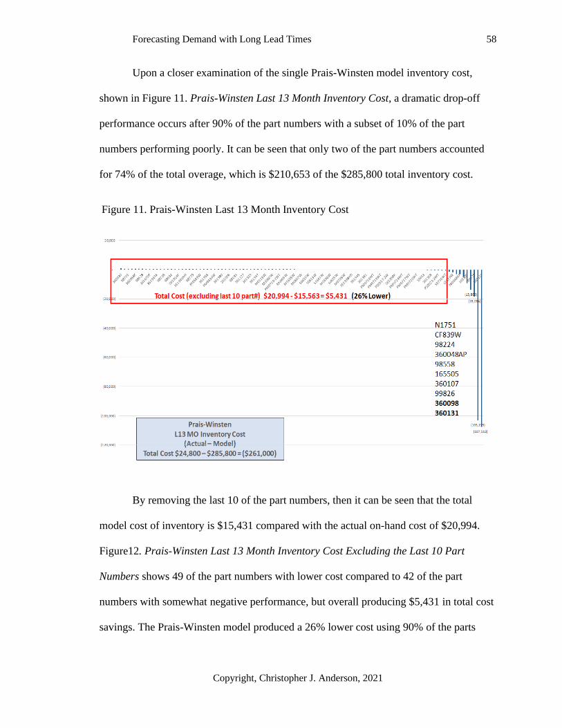
Forecasting Demand with Long Lead Times 58
Copyright, Christopher J. Anderson, 2021
Upon a closer examination of the single Prais-Winsten model inventory cost,
shown in Figure 11. Prais-Winsten Last 13 Month Inventory Cost, a dramatic drop-off
performance occurs after 90% of the part numbers with a subset of 10% of the part
numbers performing poorly. It can be seen that only two of the part numbers accounted
for 74% of the total overage, which is $210,653 of the $285,800 total inventory cost.
By removing the last 10 of the part numbers, then it can be seen that the total
model cost of inventory is $15,431 compared with the actual on-hand cost of $20,994.
Figure12. Prais-Winsten Last 13 Month Inventory Cost Excluding the Last 10 Part
Numbers shows 49 of the part numbers with lower cost compared to 42 of the part
numbers with somewhat negative performance, but overall producing $5,431 in total cost
savings. The Prais-Winsten model produced a 26% lower cost using 90% of the parts
Figure 11. Prais-Winsten Last 13 Month Inventory Cost

Forecasting Demand with Long Lead Times 59
Copyright, Christopher J. Anderson, 2021
numbers. The ten parts that were excluded appeared to exhibit non-normal behavior with
various spikes in demand. This was determined to be because of a new major account.
These spikes are illustrated in Figure 13. Part 360098 Sales Demand and
Inventory shows the non-normal demand (blue line) causing the forecasting models to
have difficulty ordering enough inventory, given the four-month lead time, to prevent
stockouts. The green line shows the model's inventory results compared to the actual
results the company experienced. The company tends to keep more inventory on hand
because of the potential stockout penalties, and it was noticed that the company did not
stock out during any of these spikes in demand.
Figure 12. Prais-Winsten Last 13 Month Inventory Cost Excluding the Last 10 Part Numbers

Forecasting Demand with Long Lead Times 60
Copyright, Christopher J. Anderson, 2021
The company explained that the spikes are caused by sales and marketing lift
promotional programs when bringing on a new account. When a major new account is
brought onboard, the company might agree to accept stock from the distributor to
refurbish or rework. Then some of this stock is sent back out to the account’s other
distribution locations. This stock is not ordered from their Asian suppliers, and the
rework is mostly repackaging, which can be done quickly to ship rapidly. The parts that
are returned may not be the same quantity as those that are shipped out, resulting in a
stock rebalancing with no significant change in total inventory because they immediately
had the stock ready to ship, and they did not have to wait four months for resupply.
In addition, the order data that was sent included a request date and a ship date.
Sometimes the customer will hold an order for four to eight weeks because their store is
not ready to receive the stock. This delay was not accounted for in the data, which means
Figure 13. Part 360098 Sales Demand and Inventory

Forecasting Demand with Long Lead Times 61
Copyright, Christopher J. Anderson, 2021
the company did have advanced notice of an order and reacted accordingly by ordering
enough inventory. The demand data used for this project included this rebalancing and
held orders, but the advanced stocking orders were not included in the prior notice data
table. Since the lift adjustment could not be made, it caused these spikes in the demand
data picture.
The use of a single forecasting model to predict future demand across several
different parts numbers can perform poorly and appears to be less robust or agile to
respond to the variation in demand even when using a sample of 100 non-intermittent and
low CV2 classified parts. It is possible that using different forms of classification, data
clustering, and demand prediction (Steuer, Hutterer, Korevaar, & Fromm, 2018) could
lead to better results. Clearly, each forecasting method is different, just like the
differences found in each of the individual part number demand patterns.
Multiple Forecasting Model Results
Choosing the optimal forecasting model for each part number produced much
better results. Table 8. Select Forecasting Model Performance shows the total inventory
cost performance of each model optimized around individual raw part numbers leading to
a significant improvement over the one-size-fits-all approach. Six of the eight or 75%
forecasting models (highlighted in red) did better than their actual performance. Again,
the few non-normal demand part numbers caused the Prais-Winsten model to perform
poorly, just like before.

Forecasting Demand with Long Lead Times 62
Copyright, Christopher J. Anderson, 2021
Figure 14. Part Number Models over the Last 13 Month Inventory Cost
Table 8. Select Forecasting Model Performance

Forecasting Demand with Long Lead Times 63
Copyright, Christopher J. Anderson, 2021
The inventory cost resulting from the performance of the individual models is
shown in Figure 14. Part Number Models over the Last 13 Month Inventory Cost. Each
part number is sorted from those that did the best to worst. The total cost excluding the
last three of the part numbers is $12,639 compared to the actual cost of $23,942, resulting
in a difference of $11,303 in savings (see Figure 15. Part Number Models Last 13 Month
Inventory Cost Excluding 3 Part Numbers) made up of 62 of the part numbers with
$13,360 lower cost and 35 of the part numbers with $2,057 in higher cost. The total is
47% lower than the company's actual performance and almost twice the performance of a
single Prais-Winsten model, which was 26%.
Using a different model for each part number is slightly more computationally
intensive. However, if this were done every month, it would not be necessary to
recompute the past months. Only the new data would need to be added each month, and
Figure 15. Part Number Models Last 13 Month Inventory Cost Excluding 3 Part Numbers

Forecasting Demand with Long Lead Times 64
Copyright, Christopher J. Anderson, 2021
the new parameters could be optimized, and possibly a new model could be selected
based on its performance that month.
Results Summary
In answer to the first research question: Do complex forecasting methods increase
forecasting accuracy? Yes, using an optimal model for individual part numbers worked
even better. Selecting the complex model Prais-Winsten as a single model over the whole
time series performed best at 96%, but it incurred 11x greater cost. If we exclude last 10
of the most volatile part numbers due to non-normal behavior, then the total model
inventory cost would be $5,431 or 26% lower than the company’s current method of
inventory control. Using the forecasting model that performed the best for an individual
part number created a total model inventory cost of $11,303 or 47% lower than their
current method of inventory control, when we exclude the last three of the part numbers
due to non-normal behavior.
In answer to the second research question: Can exogenous data improve demand
forecasting? Maybe, but using Google Trends was not significantly better. The Google
data appeared promising at the start, but after analysis, it turned out to be insignificant.
However, the Google Trends data was helpful in finding an autoregressive AR(1) process
with a first-order moving average. This indicated the use of the Prais-Winsten method, an
iterative process designed for dealing with AR(1) errors., which led to it being added as a
forecasting method in this study.
In answer to the third research question: Can stock control metrics be used to
evaluate forecast accuracy? Yes, using inventory costs is better than forecast error
because it is in dollar terms, so everyone can easily understand the impact to the bottom

Forecasting Demand with Long Lead Times 65
Copyright, Christopher J. Anderson, 2021
line. Imprecise forecasting projections are costly to businesses, resulting in stockouts and
lost revenues, as well as overstocking and failing to fulfill service level agreements
resulting in incurring penalties (Kourentzes et al., 2020). Stock control includes more
factors than looking at forecast error in terms like RMSE or MAE. Syntetos,
Nikolopoulos, and Boylan (2010) note that forecasting methods utilized as an input to
inventory control should be assessed on their effects on inventory control.
There is also the effect of safety stock, customer service expectations, and current
levels of inventory on hand that all inform the order. A business is more concerned with
the effects of forecast error on CSL and inventory levels than the value of forecast error.
Translating the forecast error into an inventory cost number provides better feedback for
stock control. The company currently tracks monthly fill rates, but it does not have a
method for order accuracy beyond their fill rate. The research results support the use of
the Prais-Winsten method for non-intermittent demand as an improved method over the
linear model they are using today. The company believes they could save even more
using optimized models for each part number.
In answer to the fourth research question: Can a procedure be developed that is
likely to be adopted? Yes. The purchasing manager currently aggregates different inputs
to inform his judgment on the final order quantity, including using the linear time trend in
an Excel spreadsheet to estimate demand in the next four months. A routine can be
developed from within MS Excel or Power BI calling an R or Python program to perform
the complex forecasting. The selected model that performs the best could be deployed
into the organization and validated against future data (periods +1, 2, 3). In each future
month, the parameters of the forecast model would be updated with the new data.

Forecasting Demand with Long Lead Times 66
Copyright, Christopher J. Anderson, 2021
Chapter 5: Discussion
The study provided a solution to demand forecasting based on predictive analytics
of automotive aftermarket company data combined with exogenous data from Google
Trends. The contribution to practice includes stock control metrics to determine forecast
accuracy and evaluate whether forecast model complexity leads to better results.
Although an improvement in forecast accuracy was not obtained by using external
Google Trends, it is still possible that other data sources could lead to such improvement.
The resulting optimal inventory policy should not be difficult to implement and
produce cost savings over the company's current method. An optimal inventory policy
would lead to lower inventory uncertainty and a significant rise in warehouse space
utilization while maintaining a high CSL demanded by customers and the company’s
marketing strategy.
The study illustrates the inadequacy of simple univariate models used for
forecasting that did not perform better than the complex models like Prais-Winsten, an
econometric model rarely used in demand forecasting for inventory control or automotive
parts. The study shows how forecast models that consider stock control metrics can
provide more significant inventory optimization over traditional accuracy measures.
Moreover, the study adds to the limited empirical research on demand forecasting using
predictive analytics with long lead times, exogenous variables, stock control metrics, and
dynamic model updating, and the use of Prais-Winsten for demand forecasting for
automotive parts.

Forecasting Demand with Long Lead Times 67
Copyright, Christopher J. Anderson, 2021
Limitations
There were a few limitations of the study based on the research design and
provided data. The company only provided 54 months of data the was usable due to a
change in accounting systems that made the older data difficult to reconcile with the new
accounting system. Utilizing more data would have allowed larger training sets for the
forecasts.
The study design focused on 100 nonintermittent sample parts in order to reduce
computational complexity; therefore, none of the intermittent parts were included in the
study. Adding intermittent part numbers would have provided greater certainty regarding
the overall inventory performance for the whole company.
Data governance was an issue with the company. There did not appear to be clear
historical records of the advanced notice data making it difficult to break out the non-
normal behavior that was known to be occurring. Also, the historical stockout costs were
estimated at 90% of profit, but the actual costs were estimated to vary by more due to
changes in customer discounts, promotions, supplier costs, and quantity purchase
discounts.
The study's final limitation stemmed from the constraints of the ‘R’ language
libraries used for computation. None of the libraries supported stock control metrics for
evaluation. The study was also unable to overcome computing cross-validation numbers
using exogenous regressors for unsupported forecasting models. Given more time, the
study could overcome some of these limitations in ‘R’ libraries or data.

Forecasting Demand with Long Lead Times 68
Copyright, Christopher J. Anderson, 2021
Extensions and Future Research
This study provides the opportunity for several future possibilities to extend these
research findings. Further research into how easily the new forecast method is adopted,
used, and performed in the future could be explored better to understand continuous
utilization, adaptation, and changes.
There were 100 non-intermittent and low CV2 classified parts. Further
exploration of the remaining intermittent and non-intermittent parts could be investigated
to determine if better performance can be obtained with new, more sophisticated, and
different models that could produce even better results.
The company’s judgment worked quite well in the past without using safety stock
in their ordering policy. Although research studies have shown the advantages of both
safety stock (Chu & Shen, 2010; Kang, Ullah, & Sarkar, 2018) and statistical forecasting
methods, businesses continue to rely on their judgment integrated with demand
forecasting, frequently described as “integrating forecasting” methods (Arvan, Fahimnia,
Reisi, & Siemsen, 2019; Baecke, De Baets, & Vanderheyden, 2017; Syntetos,
Nikolopoulos, Boylan, Fildes, & Goodwin, 2009). A model could be developed to
understand how well their current judgment performance works, both with and without
safety stock, and then integrate the existing heuristics used for forecasting judgment into
a standard ordering policy while also measuring effectiveness.
Combining several forecasts into a single model has been shown to reduce
forecasting errors and reduce the constraints inherent in a single model (Barrow &
Kourentzes, 2016). Additional research into different sources of exogenous data like

Forecasting Demand with Long Lead Times 69
Copyright, Christopher J. Anderson, 2021
using the companies own website searches, hits, or individual customer ordering patterns
might lead to additional improvement.
Understanding how automotive parts age and the production cycle is also crucial
to raw material purchasing. As automobiles age, they become less popular and expensive
to maintain, which results in demand for automotive parts declining. This results in
retailers using stock balancing of older inventory or negative demand to the
manufacturer. At the same time, as the purchasing cycle improves, it is essential for
production planning to improve and become more efficient. Significant opportunities for
improvement would exist for production planning, material handling, and inventory
usage to understand how this negative demand due to aging, along with committed raw
material parts, affects finished goods inventory. Furthermore, a replication of this study
in other firms and industries would be valuable.
There is also the use of clustering analysis to break down large groupings of data
items into smaller groups based on their similarities while considering the complex bill of
material relationships between items (Srinivasan & Moon, 1999). There is also the use of
K‑nearest‑neighbor (KNN), which Nikolopoulos, Babai, and Bozos (2016) used to
forecast intermittent automotive spare parts demand. KNN is a classification method that
identifies similarities in each object to nearby objects (named tuples) with a similarity
index. These tuples are explained by n characteristics corresponding to a place in an n-
dimensional space. The KNN method finds k tuples most similar to a particular tuple.
These classifications result in the development of clusters of objects that are comparable.
KNN can also be used to reduce the dimensionality of data in regression analysis
situations.

Forecasting Demand with Long Lead Times 70
Copyright, Christopher J. Anderson, 2021
Conclusions
Demand forecasting with long lead times is challenging to obtain an accurate
forecast. In this paper, we use the data from an automotive clutch manufacturing
company, which consisted of over 1,033 imported raw parts with lead times of four
months. Monthly forecasting of part demand resulted in an assessment of various simple
and complex forecasting methods. The comparison results show that the forecasts
obtained using a single Prais-Winsten econometric method inventory order policy with
safety stock were more accurate than those obtained by other classical forecasting
methods and produced a 26% improvement over the current company use of the linear
method that is coupled with judgment and does not use safety stock.
In addition, the forecasts obtained using the best method for individual part
numbers produced a 47% improvement over the current linear method used by the
company. The paper also shows how traditional forecast error measures were
inappropriate and that using the stock control metrics, CSL, and inventory cost is superior
for non-intermittent demand, despite their consistent usage for evaluating forecast error in
many forecasting studies. The research results support the use of the Prais-Winsten
method for non-intermittent demand with long-lead times and using multiple forecasting
models that are optimized to individual part numbers for an inventory order policy.

Forecasting Demand with Long Lead Times 71
Copyright, Christopher J. Anderson, 2021
References
Akter, S., Wamba, S. F., Gunasekaran, A., Dubey, R., & Childe, S. J. (2016). How to
improve firm performance using big data analytics capability and business
strategy alignment? International Journal of Production Economics, 182, 113-
131.
Armstrong, J. S. (2001). Evaluating Forecasting Methods. In Principles of Forecasting: A
Handbook for Researchers and Practitioners (pp. 443-472). Norwell, MA:
Kluwer Academic Publishers.
Arrow, K. J., Harris, T., & Marschak, J. (1951). Optimal Inventory Policy. Econometrica,
19(3), 250.
Arvan, M., Fahimnia, B., Reisi, M., & Siemsen, E. (2019). Integrating human judgement
into quantitative forecasting methods: A review. Omega, 86, 237-252.
Axsäter, S. (1996). Using the deterministic EOQ formula in stochastic inventory control.
Management Science, 42(6), 830-834.
Baecke, P., De Baets, S., & Vanderheyden, K. (2017). Investigating the added value of
integrating human judgement into statistical demand forecasting systems.
International Journal of Production Economics, 191, 85-96.
Barrow, D. K., & Kourentzes, N. (2016). Distributions of forecasting errors of forecast
combinations: Implications for inventory management. International Journal of
Production Economics, 177, 24-33.
Bertsimas, D., & Thiele, A. (2006). A Robust Optimization Approach to Inventory
Theory. Operations Research, 54(1), 150-168.

Forecasting Demand with Long Lead Times 72
Copyright, Christopher J. Anderson, 2021
Blackburn, R., Lurz, K., Priese, B., Göb, R., & Darkow, I.-L. (2015). A predictive
analytics approach for demand forecasting in the process industry. International
Transactions in Operational Research, 22(3), 407-428.
Boylan, J. E., Syntetos, A. A., & Karakostas, G. C. (2008). Classification for forecasting
and stock control: a case study. journal of the Operational Research Society,
59(4), 473-481.
Bozorgi, A., Pazour, J., & Nazzal, D. (2014). A new inventory model for cold items that
considers costs and emissions. International Journal of Production Economics,
155, 114-125.
Brown, R. G. (1959). Statistical forecasting for inventory control: McGraw/Hill.
Bruzda, J. (2020). Demand forecasting under fill rate constraints—The case of re-order
points. International Journal of Forecasting, 36(4), 1342-1361.
Bumblauskas, D., Nold, H., Bumblauskas, P., & Igou, A. (2017). Big data analytics:
transforming data to action. Business Process Management Journal, 23(3), 703-
720.
Cachon, G. P., & Fisher, M. (2000). Supply Chain Inventory Management and the Value
of Shared Information. Management Science, 46(8), 1032-1048.
Cárdenas-Barrón, L. E., Chung, K.-J., & Treviño-Garza, G. (2014). Celebrating a century
of the economic order quantity model in honor of Ford Whitman Harris.
International Journal of Production Economics, 155, 1-7.
doi:10.1016/j.ijpe.2014.07.002

Forecasting Demand with Long Lead Times 73
Copyright, Christopher J. Anderson, 2021
Chandra, C., & Grabis, J. (2005). Application of multi-steps forecasting for restraining
the bullwhip effect and improving inventory performance under autoregressive
demand. European Journal of Operational Research, 166(2), 337-350.
Chris, A. (2020). Top 10 Search Engines In The World. Retrieved from
https://www.reliablesoft.net/top-10-search-engines-in-the-world/
Chu, L. Y., & Shen, Z.-J. M. (2010). A Power-of-Two Ordering Policy for One-
Warehouse Multiretailer Systems with Stochastic Demand. Operations Research,
58(2), 492-502.
Chuang, C.-H., & Chiang, C.-Y. (2016). Dynamic and stochastic behavior of coefficient
of demand uncertainty incorporated with EOQ variables: An application in
finished-goods inventory from General Motors׳ dealerships. International Journal
of Production Economics, 172, 95-109.
Cohen, M. (2015). Inventory Management in the Age of Big Data. Harvard business
review.
Cortés, B. M., & Borrego, E. A. V. Service Parts Forecasting in the Automotive Sector.
Costantino, F., Di Gravio, G., Patriarca, R., & Petrella, L. (2018). Spare parts
management for irregular demand items. Omega, 81, 57-66.
Danese, P., & Kalchschmidt, M. (2011). The role of the forecasting process in improving
forecast accuracy and operational performance. International Journal of
Production Economics, 131(1), 204-214.
Dejonckheere, J., Disney, S. M., Lambrecht, M. R., & Towill, D. R. (2003). Measuring
and avoiding the bullwhip effect: A control theoretic approach. European Journal
of Operational Research, 147(3), 567-590.

Forecasting Demand with Long Lead Times 74
Copyright, Christopher J. Anderson, 2021
Dejonckheere, J., Disney, S. M., Lambrecht, M. R., & Towill, D. R. (2004). The impact
of information enrichment on the Bullwhip effect in supply chains: A control
engineering perspective. European Journal of Operational Research, 153(3), 727-
750.
Dekker, R., Pinçe, Ç., Zuidwijk, R., & Jalil, M. N. (2013). On the use of installed base
information for spare parts logistics: A review of ideas and industry practice.
International Journal of Production Economics, 143(2), 536-545.
Fantazzini, D., & Toktamysova, Z. (2015). Forecasting German car sales using Google
data and multivariate models. International Journal of Production Economics,
170, 97-135.
Fildes, R. (2006). The forecasting journals and their contribution to forecasting research:
Citation analysis and expert opinion. International Journal of Forecasting, 22(3),
415-432.
Fildes, R., & Kingsman, B. (2011). Incorporating demand uncertainty and forecast error
in supply chain planning models. journal of the Operational Research Society,
62(3), 483-500.
Fildes, R., Nikolopoulos, K., Crone, S. F., & Syntetos, A. A. (2008a). Forecasting and
Operational Research: A Review. The Journal of the Operational Research
Society, 59(9), 1150-1172. Retrieved from www.jstor.org/stable/20202189
Fildes, R., Nikolopoulos, K., Crone, S. F., & Syntetos, A. A. (2008b). Forecasting and
operational research: a review. journal of the Operational Research Society,
59(9), 1150-1172.

Forecasting Demand with Long Lead Times 75
Copyright, Christopher J. Anderson, 2021
Gao, J., Xie, Y., Cui, X., Yu, H., & Gu, F. (2018). Chinese automobile sales forecasting
using economic indicators and typical domestic brand automobile sales data: A
method based on econometric model. Advances in Mechanical Engineering,
10(2), 168781401774932.
Gardner, E. S. (1985). Exponential smoothing: The state of the art. Journal of
Forecasting, 4(1), 1-28. doi:10.1002/for.3980040103
Gardner, E. S. (2006). Exponential smoothing: The state of the art—Part II. International
Journal of Forecasting, 22(4), 637-666.
Gass, S. I., & Harris, C. M. (2000). Encyclopedia of operations research and
management science (Centennial edition). (S. I. Gass & C. M. Harris Eds. Vol.
7). Dordrecht, The Netherlands: Kluwer.
Gneiting, T. (2011). Making and Evaluating Point Forecasts. Journal of the American
Statistical Association, 106(494), 746-762.
Goodhue, D. L., & Thompson, R. L. (1995). Task-Technology Fit and Individual
Performance. MIS Quarterly, 19(2), 213-236.
Google. (2020). Google Trends Search Data, . Retrieved from
https://trends.google.com/trends/explore?date=all&geo=US&q=clutch
Govindan, K., Cheng, T. C. E., Mishra, N., & Shukla, N. (2018). Big data analytics and
application for logistics and supply chain management. Transportation Research
Part E: Logistics and Transportation Review, 114, 343-349.
Graves, S. C. (1999). A Single-Item Inventory Model for a Nonstationary Demand
Process. Manufacturing & Service Operations Management, 1(1), 50-61.

Forecasting Demand with Long Lead Times 76
Copyright, Christopher J. Anderson, 2021
Green, K. C., & Armstrong, J. S. (2015). Simple versus complex forecasting: The
evidence. Journal of Business Research, 68(8), 1678-1685.
doi:10.1016/j.jbusres.2015.03.026
Gunasekaran, A., Papadopoulos, T., Dubey, R., Wamba, S. F., Childe, S. J., Hazen, B., &
Akter, S. (2017). Big data and predictive analytics for supply chain and
organizational performance. Journal of Business Research, 70, 308-317.
Gurtu, A. (2021). Optimization of Inventory Holding Cost Due to Price, Weight, and
Volume of Items. Journal of Risk and Financial Management, 14(2), 65.
doi:10.3390/jrfm14020065
Hadley, G., & Whitin, T. M. (1963). Analysis of inventory systems. Retrieved from
Harris, F. W. (1913, February 1913). How Many Parts to Make at Once. Factory, The
Magazine of Management, 10(2), 135-136, 152.
Harris, F. W. (1990). How Many Parts to Make at Once. Operations Research, 38(6),
947-950.
Hazen, B. T., Overstreet, R. E., & Cegielski, C. G. (2012). Supply chain innovation
diffusion: going beyond adoption. The International Journal of Logistics
Management, 23(1), 119-134.
Holt, C. C. (1957). Forecasting seasonals and trends by exponentially weighted moving
averages. . International Journal of Forecasting 20, 5-10.
Hyndman, R. J., & Athanasopoulos, G. (2018). Forecasting: principles and practice:
OTexts.
Johnston, F., & Boylan, J. E. (1996). Forecasting for items with intermittent demand.
journal of the Operational Research Society, 47(1), 113-121.

Forecasting Demand with Long Lead Times 77
Copyright, Christopher J. Anderson, 2021
Kache, F., & Seuring, S. (2017). Challenges and opportunities of digital information at
the intersection of Big Data Analytics and supply chain management.
International Journal of Operations & Production Management, 37(1), 10-36.
Kang, C. W., Ullah, M., & Sarkar, B. (2018). Optimum ordering policy for an imperfect
single-stage manufacturing system with safety stock and planned backorder. The
International Journal of Advanced Manufacturing Technology, 95(1), 109-120.
Kocer, U. U. (2013). Forecasting intermittent demand by Markov chain model.
International Journal of Innovative Computing, Information and Control, 9(8),
3307-3318.
Kourentzes, N. (2014). On intermittent demand model optimisation and selection.
International Journal of Production Economics, 156, 180-190.
Kourentzes, N., Trapero, J. R., & Barrow, D. K. (2020). Optimising forecasting models
for inventory planning. International Journal of Production Economics, 225,
107597.
Lamba, K., & Singh, S. P. (2018). Modeling big data enablers for operations and supply
chain management. The International Journal of Logistics Management, 29(2),
629-658.
LaValle, S., Lesser, E., Shockley, R., Hopkins, M. S., & Kruschwitz, N. (2011). Big data,
analytics and the path from insights to value. MIT Sloan Management Review,
52(2), 21-32.
Lee, C.-C., Cheng, H. K., & Cheng, H.-H. (2007). An empirical study of mobile
commerce in insurance industry: Task–technology fit and individual differences.
Decision Support Systems, 43(1), 95-110.

Forecasting Demand with Long Lead Times 78
Copyright, Christopher J. Anderson, 2021
Lee, H. L., Padmanabhan, V., & Whang, S. (1997). The bullwhip effect in supply chains.
MIT Sloan Management Review, 38, 93-102.
Leonard, D. A. (1988). Implementation as mutual adaptation of technology and
organization. Research Policy, 17(5), 251-267.
Li, B., & Arreola-Risa, A. (2017). Financial risk, inventory decision and process
improvement for a firm with random capacity. European Journal of Operational
Research, 260(1), 183-194.
Mu, E., Kirsch, L. J., & Butler, B. S. (2015). The assimilation of enterprise information
system: An interpretation systems perspective. Information & Management,
52(3), 359-370.
Napier, R. A. (2014). Matching Inventory Replenishment Heuristics To Demand
Patterns: A Cost/benefit Approach.
Nikolopoulos, K. I., Babai, M. Z., & Bozos, K. (2016). Forecasting supply chain sporadic
demand with nearest neighbor approaches. International Journal of Production
Economics, 177, 139-148.
Peidro, D., Mula, J., Poler, R., & Lario, F.-C. (2009). Quantitative models for supply
chain planning under uncertainty: a review. The International Journal of
Advanced Manufacturing Technology, 43(3-4), 400-420.
Petropoulos, F., Wang, X., & Disney, S. M. (2019). The inventory performance of
forecasting methods: Evidence from the M3 competition data. International
Journal of Forecasting, 35(1), 251-265.
Prais, S. J., & Winsten, C. B. (1954). Trend estimators and serial correlation. Retrieved
from Cowles Commission Discussion Paper, 383 (Chicago):

Forecasting Demand with Long Lead Times 79
Copyright, Christopher J. Anderson, 2021
Qin, Y., & Yun, C. (2012). Auto Parts Demand Forecasting Based on Nonnegative
Variable Weight Combination Model in Auto Aftermarket. Paper presented at the
2012 International Conference on Management Science & Engineering (19th),
Dallas, USA.
R Core Team. (2013). R: A language and environment for statistical computing. Vienna,
Austria: R Foundation for Statistical Computing. Retrieved from http://www.R-
project.org/
Rao, U. S. (2003). Properties of the Periodic Review (R, T) Inventory Control Policy for
Stationary, Stochastic Demand. Manufacturing & Service Operations
Management, 5(1), 37-53.
Rego, J. R. D., & Mesquita, M. A. D. (2015). Demand forecasting and inventory control:
A simulation study on automotive spare parts. International Journal of
Production Economics, 161, 1-16.
Rezaei, J. (2014). Economic order quantity for growing items. International Journal of
Production Economics, 155, 109-113.
Sagaert, Y. R., Kourentzes, N., Vuyst, S. D., Aghezzafa, E.-H., & Desmet, B. (2018).
Incorporating macroeconomic leading indicators in tactical capacity planning.
International Journal of Production Economics, 209, 12-19.
Sana, S. S. (2011). The stochastic EOQ model with random sales price. Applied
Mathematics and Computation, 218(2), 239-248.
Sanders, N., & Graman, G. (2009). Quantifying costs of forecast errors: A case study of
the warehouse environment☆. Omega: International Journal of Management
Science, 37(1), 116-125.

Forecasting Demand with Long Lead Times 80
Copyright, Christopher J. Anderson, 2021
Sarkar, B., & Moon, I. (2014). Improved quality, setup cost reduction, and variable
backorder costs in an imperfect production process. International Journal of
Production Economics, 155, 204-213.
Scarf, H. (1959). The optimality of (5, 5) policies in the dynamic inventory problem.
Optimal pricing, inflation, and the cost of price adjustment.
Schwarz, L. B. (2008). The economic order-quantity (EOQ) model. In Building Intuition
(pp. 135-154): Springer.
Sicilia, J., González-De-La-Rosa, M., Febles-Acosta, J., & Alcaide-López-De-Pablo, D.
(2014). An inventory model for deteriorating items with shortages and time-
varying demand. International Journal of Production Economics, 155, 155-162.
Silver, E. A., & Bischak, D. P. (2011). The exact fill rate in a periodic review base stock
system under normally distributed demand. Omega, 39(3), 346-349.
Silver, E. A., Pyke, D. F., & Peterson, R. (1998). Inventory management and production
planning and scheduling (Vol. 3): Wiley, New York, NY.
Singh, D., & Verma, A. (2018). Inventory Management in Supply Chain. Materials
Today: Proceedings, 5(2), 3867-3872.
Smith, W., Coleman, S., Bacardit, J., & Coxon, S. (2018). How data can change the
automotive aftermarket. Focus.
Smith, W., Coleman, S., Bacardit, J., & Coxon, S. (2019). Insight from data analytics
with an automotive aftermarket SME. Quality and Reliability Engineering
International(35), 1396–1407.
Snyder, L. V. (2014). A tight approximation for an EOQ model with supply disruptions.
International Journal of Production Economics, 155, 91-108.

Forecasting Demand with Long Lead Times 81
Copyright, Christopher J. Anderson, 2021
Souza, G. C. (2014). Supply chain analytics. Business Horizons, 57(5), 595-605.
Sphicas, G. P. (2014). Generalized EOQ formula using a new parameter: Coefficient of
backorder attractiveness. International Journal of Production Economics, 155,
143-147.
Srinivasan, M., & Moon, Y. B. (1999). A comprehensive clustering algorithm for
strategic analysis of supply chain networks. Computers & Industrial Engineering,
36(3), 615-633.
Steuer, D., Hutterer, V., Korevaar, P., & Fromm, H. (2018). A similarity-based approach
for the all-time demand prediction of new automotive spare parts.
Strasheim, J. J. (1992). Demand Forecasting For Motor Vehicle Spare Parts. The South
African Journal of Industrial Engineering, 6(2), 18-29.
Strijbosch, L. W. G., Syntetos, A. A., Boylan, J. E., & Janssen, E. (2011). On the
interaction between forecasting and stock control: The case of non-stationary
demand. 133(1), 470-480.
Syntetos, A. A., & Boylan, J. E. (2001). On the bias of intermittent demand estimates.
International Journal of Production Economics, 71(1-3), 457-466.
Syntetos, A. A., & Boylan, J. E. (2005). The accuracy of intermittent demand estimates.
International Journal of Forecasting, 21(2), 303-314.
Syntetos, A. A., & Boylan, J. E. (2006). On the stock control performance of intermittent
demand estimators. International Journal of Production Economics, 103(1), 36-
47.
Syntetos, A. A., Boylan, J. E., & Croston, J. (2005). On the categorization of demand
patterns. journal of the Operational Research Society, 56(5), 495-503.

Forecasting Demand with Long Lead Times 82
Copyright, Christopher J. Anderson, 2021
Syntetos, A. A., Nikolopoulos, K., & Boylan, J. E. (2010). Judging the judges through
accuracy-implication metrics: The case of inventory forecasting. International
Journal of Forecasting, 26(1), 134-143.
Syntetos, A. A., Nikolopoulos, K., Boylan, J. E., Fildes, R., & Goodwin, P. (2009). The
effects of integrating management judgement into intermittent demand forecasts.
International Journal of Production Economics, 118(1), 72-81.
Taleizadeh, A. A., & Pentico, D. W. (2014). An Economic Order Quantity model with
partial backordering and all-units discount. International Journal of Production
Economics, 155, 172-184.
Tashman, L. J. (2000). Out-of-sample tests of forecasting accuracy: an analysis and
review. International Journal of Forecasting, 16(4), 437-450.
Teksan, Z. M., & Geunes, J. (2016). An EOQ model with price-dependent supply and
demand. International Journal of Production Economics, 178, 22-33.
Teunter, R. H., & Duncan, L. (2009). Forecasting intermittent demand: a comparative
study. journal of the Operational Research Society, 60(3), 321-329.
Tiacci, L., & Saetta, S. (2009). An approach to evaluate the impact of interaction between
demand forecasting method and stock control policy on the inventory system
performances. International Journal of Production Economics, 118(1), 63-71.
Van Der Auweraer, S., Boute, R. N., & Syntetos, A. A. (2019). Forecasting spare part
demand with installed base information: A review. International Journal of
Forecasting, 35(1), 181-196.

Forecasting Demand with Long Lead Times 83
Copyright, Christopher J. Anderson, 2021
Vargas, V. (2009). An optimal solution for the stochastic version of the Wagner–Whitin
dynamic lot-size model. European Journal of Operational Research, 198(2), 447-
451.
Verma, S., Bhattacharyya, S. S., & Kumar, S. (2018). An extension of the technology
acceptance model in the big data analytics system implementation environment.
Information Processing & Management, 54(5), 791-806.
Wagner, H. M., & Whitin, T. M. (1958). Dynamic version of the economic lot size
model. Management Science, 5(1), 89-96.
Wang, G., Gunasekaran, A., Ngai, E. W. T., & Papadopoulos, T. (2016). Big data
analytics in logistics and supply chain management: Certain investigations for
research and applications. International Journal of Production Economics, 176,
98-110.
Waters, D. (2008). Inventory control and management: John Wiley & Sons.
Wilson, R. (1934). A scientific routine for stock control: Harvard Univ.
Zheng, Y.-S. (1992). On properties of stochastic inventory systems. Management
Science, 38(1), 87-103.
Zinn, W., & Marmorstein, H. (1990). Comparing two alternative methods of determining
safety stock levels: The demand and the forecast systems. Journal of Business
Logistics, 11(1), 95.

Forecasting Demand with Long Lead Times 84
Copyright, Christopher J. Anderson, 2021
Appendix – R Program Code
# Load Libraries
library(forecast)
library(prais)
library(smooth)
###START
# LOOP all SKUs using Exogenous regressors
xreg_sw <- "FALSE"
for (sw in (1:2)) { # xreg_sw loop
#load company dataframe from excel delimited
Company.df = read.delim("Data_inv_sales_not100cv-smooth.txt", header = TRUE)
last <- 54
#Replace missing data with "0"
Company.df[Company.df==""] <- 0
demand_o.v <<- vector("integer", length = last)
onhand_inv.v <<- vector("integer", length = last)
notice.v <<- vector("integer", length = last)
date.v <<- seq(as.Date("2016-1-1"), as.Date("2020-6-1"), by = "months")
#load Google dataframe from excel delimited
Google.df = read.delim("GoogleTrends.txt", header = TRUE)
Gtrends.v <- vector("integer", length = last)
Gtrends.v <- as.integer(Google.df[1:last])
Gwin.ts <<- ts(Gtrends.v, start=c(2016,1), freq=12)
eXreg <- "GoogleTrends"
N <- 100 # total SKU 100
results.df = data.frame(
sku = character(N),
cost = numeric(N),
price = numeric(N),
Hcsl = numeric(N),
MHcsl = character(N),
MCSLmethod = character(N),
MTinvC = numeric(N),
LcvRMSE = numeric(N),
McvRMSE = character(N),
RMSETinvC = numeric(N),
Laic = numeric(N),
Maic = character(N),

Forecasting Demand with Long Lead Times 85
Copyright, Christopher J. Anderson, 2021
aicTinvC = numeric(N),
MTinv_Tgtcsl= numeric(N),
MTinv_Tgt = character(N), #Model of Lowest Inv to meet Target CSL
MCSLmethTgt = character(N),
MTinv_TgtC = numeric(N),
Act_invC = numeric(N),
L13_CSL = numeric(N),
L13_invC = numeric(N),
L13_ActinvC = numeric(N),
L13_MTinv = character(N),
L13_avg = numeric(N),
L13_sd = numeric(N),
L13_cv2 = numeric(N),
L_avg = numeric(N),
L_sd = numeric(N),
L_cv2 = numeric(N),
hz = integer(N),
win = integer(N),
eXreg = character(N),
fill_rate = numeric(N)
)
irate <- 0.05/12 # annual interest rate
discount <- -0.9 # % of profit for backorder
fill_rate <- 0.99
win <<- 12 # 12-period rolling window
hz <<- 4 # 4-period forecast lead time
stwin <<- 12 # start window ignores first 12 mo
mo.v <<- rep(1:12,5)
mo.v <<- mo.v[1:54]
mo_sq.v <<- mo.v * mo.v
Nmo.v <<- seq(54)
Nmo.ts <<- ts(Nmo.v, start=c(2016,1), freq=12)
#model "N"=none, "A"=additive, "M"=multiplicative, Ad=AdditiveDamped,
"Z"=automatically selected and "C"=combine
# CV Forecast Methods
flm <- function(y, h) {
df <- data.frame(fwin.cv, Mwin.cv)
mod <- alm(fwin.cv ~ Mwin.cv, df, distribution="dnorm")
forecast(mod,h=hz,interval="p")
}
flmp <- function(y, h) {
df <- data.frame(y, Mwin.cv)
mod <- alm(demand.ts ~ Mwin.cv, df, distribution="dpois")
forecast(mod,h=hz,interval="p")

Forecasting Demand with Long Lead Times 86
Copyright, Christopher J. Anderson, 2021
}
fses <- function(y, h) { forecast(es(y, model="ANN"), h=h) }
fdes <- function(y, h) { forecast(es(y, model="AAN"), h=h) }
ftes <- function(y, h) { forecast(es(y, model="ZZN"), h=h) }
fma <- function(y, h) { forecast(sma(y, win), h=h) }
fpw <- function(y, h, x1, x2, x3) { forecast(prais_winsten(y ~ x1 + x2, data=x3), h=h) }
fgpw <- function(y, h, x1, x2, x3, xreg) { forecast(prais_winsten(y ~ x1 + x2 + xreg,
data=x3), h=h,interval="p") }
fglm <- function(y, h, xreg) {
df <- data.frame(fwin.cv, Mwin.cv, Gwin.cv)
mod <- alm(fwin.cv ~ Mwin.cv+Gwin.cv, df, distribution="dnorm")
forecast(mod,h=hz,interval="p")
}
fglmp <- function(y, h, xreg) {
df <- data.frame(y, Mwin.cv, xreg)
mod <- alm(y ~ Mwin.cv+xreg, df, distribution="dpois")
forecast(mod,h=hz,interval="p")
}
fgses <- function(y, h, xreg, newxreg) { forecast(es(y, model="ANN", holdout=FALSE,
xreg=xreg), h=h) }
fgdes <- function(y, h, xreg, newxreg) { forecast(es(y, model="AAN", holdout=FALSE,
xreg=xreg), h=h) }
fgtes <- function(y, h, xreg, newxreg) { forecast(es(y, model="ZZN", holdout=FALSE,
xreg=xreg), h=h) }
mean_fcst <- function(y, h, n) {
fcst <<- predict(y,h=h,interval="p")
forecast.v[n+1] <<- round(fcst$mean[h], digits=0)
Pforecast.v[n+1]<<- round(sum(fcst$mean[1:h]), digits=0) # 4-period forecast sum
for (i in seq(h)) { Pfcst.mat[n+1,i] <<- fcst$mean[i] }
return(round(fcst$mean[h], digits=0))
}
#LOOP through part number SKUs
for (f in (1:N)) {
#load vectors with company SKU data
RM <<- as.character(Company.df[f,1])
cost <<- as.numeric(Company.df[f,2])
price <<- as.numeric(Company.df[f,3])
demand_o.v <<- as.integer(Company.df[f,4:57])
notice.v <<- as.integer(Company.df[f,58:111])
onhand_inv.v <<- as.integer(Company.df[f,112:165])

Forecasting Demand with Long Lead Times 87
Copyright, Christopher J. Anderson, 2021
profit <- price - cost
part.v <<- c(RM, cost, price, profit)
CSL.df <<- data.frame(
model_name.v = c("Naive", "Naive Drift", "Brown SES","Holt DES","Holt
DESZ","Linear","Moving Average","Prais Winsten"),
CSL = 0.0,
inv_low = 0,
inv_high = 0,
inv_rang = 0,
cvME = 0.0,
cvRMSE = 0.0,
cvMAE = 0.0,
aic = 0.0,
method = "NA",
Tinv_neg = 0.0,
Tinv_pos = 0.0,
Tinv = 0.0,
Tinv_negC= 0.0,
Tinv_posC= 0.0,
TinvC = 0.0,
ActinvC = 0.0,
L13_CSL = 0.0,
L13_invC = 0.0,
L13_ActinvC = 0.0,
L13_MTinv_Tgt = " "
)
# Initialize Start Conditions
demand.v <<- demand_o.v - notice.v
start <- round(mean(demand.v[1:12]), digits=0)
demand.ts <- ts(demand.v, start=c(2016,1), freq=12)
#LOOP through Methods
write.table(RM, "results.csv", sep = ",", col.names = TRUE, append = T)
for (fn in (1:8)) {
# Initialize Vectors
forecast.v <<- vector("integer", length = last)
level.v <<- vector("integer", length = last)
trend.v <<- vector("integer", length = last)
season.v <<- vector("integer", length = last)
alpha.v <<- vector("integer", length = last)
beta.v <<- vector("integer", length = last)
method.v <<- vector("character", length = last)

Forecasting Demand with Long Lead Times 88
Copyright, Christopher J. Anderson, 2021
SS.v <<- vector("integer", length = last)
order.v <<- vector("integer", length = last)
ExpInvB4_order.v <<- vector("integer", length = last)
delivery.v <<- vector("integer", length = last)
EOP_Inv.v <<- vector("integer", length = last)
forecast_err.v <<- vector("integer", length = last)
order_err.v <<- vector("integer", length = last)
Inv_err.v <<- vector("integer", length = last)
Psim_fc.v <<- vector("integer", length = last)
Pforecast.v <<- vector("integer", length = last)
Pfcst.mat <<- matrix(0, nrow = last, ncol = 5)
forecast.v[1] <- start
Pforecast.v[1] <- forecast.v[1]*hz
SS.v[1:5] <- round(qnorm(fill_rate) * sd(demand.v[1:12]), digits=0)
order.v[1] <- start
ExpInvB4_order.v[1] <- start
delivery.v[1] <- start
# delivery.v[1:(hz+1)] <- start
for (d in (1:3)) { delivery.v[d+1] <- onhand_inv.v[d+1] - (onhand_inv.v[d] -
demand_o.v[d+1]) }
EOP_Inv.v[1] <- onhand_inv.v[1]
order_err.v[1] <- order.v[1] - demand.v[1]
Inv_err.v[1] <- EOP_Inv.v[1] - demand.v[1]
message(paste("SKU", f, RM, "method loop", fn, CSL.df$model_name.v[fn],
"Xreg=", xreg_sw, "start=", start, "Fill Rate:", fill_rate))
write.table(paste(RM, "method loop", fn, CSL.df$model_name.v[fn]), "results.csv",
sep = ",", col.names = TRUE, append = T)
# Loop through orders(n)
for (n in (1:(last-1))) {
fwin <<- window(demand.ts, end=2016+(n-1)/12)
Gwin <<- window(Gwin.ts,end=2016+(n-1)/12)
Mwin <<- window(Nmo.ts, end=2016+(n-1)/12)
if (xreg_sw == "TRUE") demand.df <<- data.frame(demand.v[1:n], mo.v[1:n],
mo_sq.v[1:n], Gtrends.v[1:n])
else demand.df <<- data.frame(demand.v[1:n], mo.v[1:n], mo_sq.v[1:n])
if (fn == "1") { # Naive
fit1 <- rwf(fwin)
mean_fcst(fit1, hz, n)
} else if (fn == "2") { #Niave w/Drift
if (n == "1") { # cannot forecast a single period
forecast.v[n+1] <- start
Pforecast.v[n+1] <- forecast.v[n+1]*hz
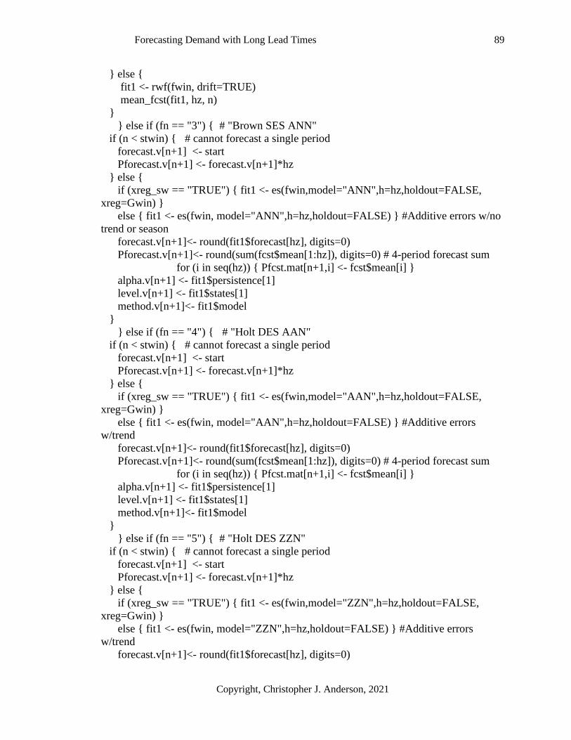
Forecasting Demand with Long Lead Times 89
Copyright, Christopher J. Anderson, 2021
} else {
fit1 <- rwf(fwin, drift=TRUE)
mean_fcst(fit1, hz, n)
}
} else if (fn == "3") { # "Brown SES ANN"
if (n < stwin) { # cannot forecast a single period
forecast.v[n+1] <- start
Pforecast.v[n+1] <- forecast.v[n+1]*hz
} else {
if (xreg_sw == "TRUE") { fit1 <- es(fwin,model="ANN",h=hz,holdout=FALSE,
xreg=Gwin) }
else { fit1 <- es(fwin, model="ANN",h=hz,holdout=FALSE) } #Additive errors w/no
trend or season
forecast.v[n+1]<- round(fit1$forecast[hz], digits=0)
Pforecast.v[n+1]<- round(sum(fcst$mean[1:hz]), digits=0) # 4-period forecast sum
for (i in seq(hz)) { Pfcst.mat[n+1,i] <- fcst$mean[i] }
alpha.v[n+1] <- fit1$persistence[1]
level.v[n+1] <- fit1$states[1]
method.v[n+1]<- fit1$model
}
} else if (fn == "4") { # "Holt DES AAN"
if (n < stwin) { # cannot forecast a single period
forecast.v[n+1] <- start
Pforecast.v[n+1] <- forecast.v[n+1]*hz
} else {
if (xreg_sw == "TRUE") { fit1 <- es(fwin,model="AAN",h=hz,holdout=FALSE,
xreg=Gwin) }
else { fit1 <- es(fwin, model="AAN",h=hz,holdout=FALSE) } #Additive errors
w/trend
forecast.v[n+1]<- round(fit1$forecast[hz], digits=0)
Pforecast.v[n+1]<- round(sum(fcst$mean[1:hz]), digits=0) # 4-period forecast sum
for (i in seq(hz)) { Pfcst.mat[n+1,i] <- fcst$mean[i] }
alpha.v[n+1] <- fit1$persistence[1]
level.v[n+1] <- fit1$states[1]
method.v[n+1]<- fit1$model
}
} else if (fn == "5") { # "Holt DES ZZN"
if (n < stwin) { # cannot forecast a single period
forecast.v[n+1] <- start
Pforecast.v[n+1] <- forecast.v[n+1]*hz
} else {
if (xreg_sw == "TRUE") { fit1 <- es(fwin,model="ZZN",h=hz,holdout=FALSE,
xreg=Gwin) }
else { fit1 <- es(fwin, model="ZZN",h=hz,holdout=FALSE) } #Additive errors
w/trend
forecast.v[n+1]<- round(fit1$forecast[hz], digits=0)

Forecasting Demand with Long Lead Times 90
Copyright, Christopher J. Anderson, 2021
Pforecast.v[n+1]<- round(sum(fcst$mean[1:hz]), digits=0) # 4-period forecast sum
for (i in seq(hz)) { Pfcst.mat[n+1,i] <- fcst$mean[i] }
alpha.v[n+1] <- fit1$persistence[1]
level.v[n+1] <- fit1$states[1]
method.v[n+1]<- fit1$model
}
} else if (fn == "6") { # "Linear"
if (n < stwin) { # cannot forecast a single period
forecast.v[n+1] <- start
Pforecast.v[n+1] <- forecast.v[n+1]*hz
Pfcst.mat[ n+1,1:(hz+1)] <- forecast.v[n+1]
} else {
if (xreg_sw == "TRUE") {
df <- data.frame(fwin, Mwin, Gwin)
fit1 <- alm(fwin~Mwin+Gwin, df,distribution="dnorm")
} else {
df <- data.frame(fwin, Mwin)
fit1 <- alm(fwin~Mwin,df,distribution="dnorm")
}
mean_fcst(fit1, hz, n)
}
} else if (fn == "7") { # SMA
if (n < stwin) { # cannot forecast a single period
forecast.v[n+1] <- start
Pforecast.v[n+1] <- forecast.v[n+1]*hz
} else {
if (n < win) { num = n } else { num = win }
fit1 <- sma(fwin, num, h=hz)
forecast.v[n+1]<- round(fit1$forecast[hz], digits=0)
Pforecast.v[n+1]<- round(sum(fit1$forecast[1:hz]), digits=0) # 4-period forecast sum
for (i in seq(hz)) { Pfcst.mat[n+1,i] <- fcst$mean[i] }
}
} else if (fn == "8") { # "Prais Winsten"
if (n < stwin) { # cannot forecast a single period
forecast.v[n+1] <- start
Pforecast.v[n+1] <- forecast.v[n+1]*hz
} else {
if (xreg_sw == "TRUE") {
fit1 <- prais_winsten(demand.v[1:n] ~ mo.v[1:n]+mo_sq.v[1:n]+ Gtrends.v[1:n],
data=demand.df)
b4 <- fit1$coefficients[4] # Gtrends.v
} else {
fit1 <- prais_winsten(demand.v[1:n] ~ mo.v[1:n]+mo_sq.v[1:n], data=demand.df)
}
e <- summary(fit1)

Forecasting Demand with Long Lead Times 91
Copyright, Christopher J. Anderson, 2021
dw <- e$dw[1] # Durbin-Watson statistic 2< autocorrelation (AC), 0=No AC, >2
Neg AC
method.v[n+1] <- paste("DW=", round(dw, digits=2))
rho<- fit1$rho[length(fit1$rho)]
b1 <- fit1$coefficients[1] # intercept
b2 <- fit1$coefficients[2] # mo.v
b3 <- fit1$coefficients[3] # mo_sq.v
if ( n > 53) {
forecast.v[n+1] <- 0
Pfcst.mat[ n+1,] <- 0
} else if (xreg_sw == "TRUE") {
err <- demand.v[n] - (rho * demand.v[n-1]) - ((1-rho) * b1) - (b2 * (mo.v[n] - rho *
mo.v[n-1])) - (b3 * (mo_sq.v[n] - rho * mo_sq.v[n-1])) - (b4 * (Gtrends.v[n] - rho *
Gtrends.v[n-1]))
forecast.v[n+1] <- round(I(rho^hz)*err + b1 + b2 * mo.v[n+1] + b3 * mo_sq.v[n+1]
+ b4 * Gtrends.v[n+1] + 0.5, digits=0)
for (i in seq(hz)) {
Pfcst.mat[ n+1,i] <- round(I(rho^i)*err + b1 + b2 * mo.v[n+i] + b3 *
mo_sq.v[n+i] + (b4 * Gtrends.v[n+1]) + 0.5, digits=0)
}
} else {
err <- demand.v[n] - (rho * demand.v[n-1]) - ((1-rho) * b1) - (b2 * (mo.v[n] - rho *
mo.v[n-1])) - (b3 * (mo_sq.v[n] - rho * mo_sq.v[n-1]))
forecast.v[n+1] <- round(I(rho^hz)*err + b1 + b2 * mo.v[n+1] + b3 * mo_sq.v[n+1]
+ 0.5, digits=0)
for (i in seq(hz)) {
Pfcst.mat[ n+1,i] <- round(I(rho^i)*err + b1 + b2 * mo.v[n+i] + b3 *
mo_sq.v[n+i] + 0.5, digits=0)
}
}
Pforecast.v[n+1] <- round(sum(Pfcst.mat[ n+1,1:hz]), digits=0)
}
} # end model IF
if (n > hz) { forecast_err.v[n] <- forecast.v[n-hz] - demand.v[n]} # cannot determine
error of last data points beyound hz (no demand)
else { forecast_err.v[n] <- forecast.v[n] - demand.v[n+hz] }
order_err.v[1] <- order.v[n] - demand.v[n]
if (n > hz) {
SS.v[n+1] <- round(qnorm(fill_rate) * sd(forecast_err.v[(n-hz):n]) + .5, digits=0)
delivery.v[n+1] <- order.v[n-(hz-1)]
ExpInvB4_order.v[n+1] <- EOP_Inv.v[n] + sum(order.v[(n-(hz-1)):n]) -
Pforecast.v[n+1] - sum(notice.v[(n-(hz-1)):n])

Forecasting Demand with Long Lead Times 92
Copyright, Christopher J. Anderson, 2021
} else { # n < hz
delivery.v[(n+hz)] <- order.v[n]
ExpInvB4_order.v[n+1] <- EOP_Inv.v[n] + sum(delivery.v[(n+1):(n+hz)]) -
Pforecast.v[n+1] - sum(notice.v[(n+1):(n+hz)])
}
order.v[n+1] <- max((forecast.v[n+1] + SS.v[n+1] - ExpInvB4_order.v[n+1]),0)
order_err.v[n+1] <- order.v[n+1] - demand.v[n+1]
EOP_Inv.v[n+1] <- EOP_Inv.v[n] + delivery.v[n+1] - demand_o.v[n+1]
Inv_err.v[n+1] <- EOP_Inv.v[n+1] - demand.v[n+1]
} # End order loop
forecast_err.v[n+1] <- 0
#Output Model Detail
print(part.v)
if (xreg_sw == "TRUE") {
ordering.df <- data.frame(date.v, demand_o.v, notice.v, forecast.v, SS.v, order.v,
ExpInvB4_order.v, delivery.v, EOP_Inv.v, forecast_err.v, Pforecast.v, alpha.v, beta.v,
method.v, level.v, trend.v, onhand_inv.v, Gtrends.v)
} else {
ordering.df <- data.frame(date.v, demand_o.v, notice.v, forecast.v, SS.v, order.v,
ExpInvB4_order.v, delivery.v, EOP_Inv.v, forecast_err.v, Pforecast.v, alpha.v, beta.v,
method.v, level.v, trend.v, onhand_inv.v)
}
print(ordering.df)
write.table(ordering.df, "results.csv", sep = ",", col.names = TRUE, row.names=FALSE,
append = T)
# Determine CV Errors
fwin.cv <<- window(demand.ts, start=2017, end=2016+last/12)
Gwin.cv <<- window(Gwin.ts,start=2017, end=2016+last/12)
Mwin.cv <<- window(Nmo.ts, start=2017, end=2016+last/12)
mo_sq.cv<<- Mwin.cv * Mwin.cv
if (xreg_sw == "TRUE") demand.df <<- data.frame(fwin.cv[13:n], Mwin.cv[13:n],
mo_sq.cv[13:n], Gwin.cv[13:n])
else demand.df <<- data.frame(fwin.cv[13:n], Mwin.cv[13:n], mo_sq.cv[13:n])
if (fn == "1") {
err <- tsCV(fwin.cv, rwf, h=hz, window=win) # Naive
} else if (fn == "2") {
err <- tsCV(fwin.cv, rwf, drift=TRUE, h=hz, window=win) #Naive Drift
} else if (fn == "3") {
if (xreg_sw == "TRUE") { err <- tsCV(fwin.cv, fgses, h=hz, window=win,
xreg=Gwin.cv) }
else { err <- tsCV(fwin.cv, fses, h=hz, window=win) } #Brown SES
} else if (fn == "4") {

Forecasting Demand with Long Lead Times 93
Copyright, Christopher J. Anderson, 2021
if (xreg_sw == "TRUE") { err <- tsCV(fwin.cv, fgdes, h=hz, window=win,
xreg=Gwin.cv) }
else { err <- tsCV(fwin.cv, fdes, h=hz, window=win) } #Holt DES
} else if (fn == "5") {
if (xreg_sw == "TRUE") { err <- tsCV(fwin.cv, fgtes, h=hz, window=win,
xreg=Gwin.cv) }
else { err <- tsCV(fwin.cv, ftes, h=hz, window=win) } #Holt DESZ
} else if (fn == "6") {
if (xreg_sw == "TRUE") { err <- tsCV(fwin.cv, fglm, h=hz, window=win,
xreg=Gwin.cv) }
else { err <- tsCV(fwin.cv, flm, h=hz, window=win) } #Linear
} else if (fn == "7") {
err <- tsCV(fwin.cv, fma, h=hz, window=win) #Moving AVG
} else if (fn == "8") {
if (xreg_sw == "TRUE") { err <- tsCV(fwin.cv, fgpw, h=hz, window=win,
x1=Mwin.cv, x2=mo_sq.cv, x3=demand.df, xreg=Gwin.cv) }
else { err <- tsCV(fwin.cv, fgpw, h=hz, window=win, x1=Mwin.cv, x2=mo_sq.cv,
x3=demand.df) } #PW
}
Arange.v <- onhand_inv.v[win:last]
ActinvC <- (sum(Arange.v[Arange.v>0]) * cost * irate) + (sum(Arange.v[Arange.v<0])
* profit * discount)
results.df$Act_invC[f] <- ActinvC
CSL.df$ActinvC[fn] <- ActinvC
CSL.df$method[fn] <- method.v[last]
CSL.df$cvRMSE[fn] <- signif(sqrt(mean(err^2, na.rm=TRUE)),digits=6)
CSL.df$cvMAE[fn] <- signif(mean(abs(err), na.rm=TRUE),digits=6)
CSL.df$cvME[fn] <- signif(mean(err, na.rm=TRUE),digits=6)
idemand.v <- demand.v[win:last]
irange.v <- EOP_Inv.v[win:last]
CSL.df$inv_low[fn] <- min(irange.v)
CSL.df$inv_high[fn]<- max(irange.v)
CSL.df$Tinv_neg[fn] <- sum(irange.v[irange.v<0])
CSL.df$Tinv_pos[fn] <- sum(irange.v[irange.v>0])
CSL.df$Tinv[fn] <- CSL.df$Tinv_pos[fn] - CSL.df$Tinv_neg[fn]
CSL.df$Tinv_negC[fn] <- CSL.df$Tinv_neg[fn] * profit * discount
CSL.df$Tinv_posC[fn] <- CSL.df$Tinv_pos[fn] * cost * irate
CSL.df$TinvC[fn] <- CSL.df$Tinv_posC[fn] + CSL.df$Tinv_negC[fn]
CSL.df$inv_rang[fn]<- abs(min(irange.v) - max(irange.v))

Forecasting Demand with Long Lead Times 94
Copyright, Christopher J. Anderson, 2021
CSL.df$CSL[fn] <- (sum(idemand.v) + sum(irange.v[irange.v<0], na.rm = TRUE)) /
sum(idemand.v)
if (fn < 3) { # Naive
CSL.df$aic[fn] <- 0
} else if (fn < 6) { # ES
CSL.df$aic[fn] <- signif(fit1$ICs[1],digits=5)
} else if (fn < 7) { # Linear
CSL.df$aic[fn] <- signif(AIC(fit1),digits=5)
} else if (fn < 8) { # SMA
CSL.df$aic[fn] <- signif(fit1$ICs[1],digits=5)
} else if (fn < 9) { # Prais-Winsten
CSL.df$aic[fn] <- c("NA")
} else if (fn < 10) { # lm w/Poisson Distribution
CSL.df$aic[fn] <- signif(AIC(fit1),digits=5)
}
irange_len <- length(irange.v)
sub_irange.v <- irange.v[(irange_len-12):irange_len]
CSL.df$L13_CSL[fn] <- (sum(idemand.v[(irange_len-12):irange_len], na.rm = TRUE)
+ sum(sub_irange.v[sub_irange.v<0], na.rm = TRUE)) / sum(idemand.v[(irange_len-
12):irange_len], na.rm = TRUE)
CSL.df$L13_invC[fn] <- (sum(sub_irange.v[sub_irange.v>0], na.rm = TRUE) * cost *
irate) + (sum(sub_irange.v[sub_irange.v<0], na.rm = TRUE) * profit * discount)
sub_onhand_inv.v <- onhand_inv.v[(last-12):last]
L13_ActinvC <- (sum(sub_onhand_inv.v[sub_onhand_inv.v>0], na.rm = TRUE)
* cost * irate) + (sum(sub_onhand_inv.v[sub_onhand_inv.v<0], na.rm = TRUE) * profit
* discount)
CSL.df$L13_ActinvC[fn] <- L13_ActinvC
} # End method loop
#Descriptive Statistics
results.df$sku[f] <- RM
results.df$cost[f] <- cost
results.df$price[f] <- price
results.df$fill_rate[f] <- fill_rate
maxCSL <- which.max(CSL.df$CSL)
results.df$Hcsl[f] <- max(CSL.df$CSL)
results.df$MHcsl[f] <- CSL.df$model_name[maxCSL]
results.df$MCSLmethod[f]<- CSL.df$method[maxCSL]
results.df$MTinvC[f] <- CSL.df$TinvC[maxCSL]

Forecasting Demand with Long Lead Times 95
Copyright, Christopher J. Anderson, 2021
minRMSE <- which.min(CSL.df$cvRMSE)
results.df$LcvRMSE[f] <- CSL.df$cvRMSE[minRMSE]
results.df$McvRMSE[f] <- CSL.df$model_name[minRMSE]
results.df$RMSETinvC[f] <- CSL.df$TinvC[minRMSE]
minaic <- which.min(CSL.df$aic[3:7])
results.df$Laic[f] <- min(CSL.df$aic[3:7])
results.df$Maic[f] <- CSL.df$model_name[minaic]
results.df$aicTinvC[f] <- CSL.df$TinvC[minaic]
results.df$HTinv_neg[f] <- max(CSL.df$Tinv_neg)
results.df$LTinv_pos[f] <- min(CSL.df$Tinv_pos)
results.df$LTinv[f] <- min(CSL.df$Tinv)
Tinv_sort <- order(CSL.df$TinvC)
target <- 0.944
for (x in (1:length(Tinv_sort))){
if (CSL.df$CSL[Tinv_sort[x]] > target) {
results.df$MTinv_Tgtcsl[f] <- CSL.df$CSL[Tinv_sort[x]]
results.df$MTinv_Tgt[f] <- CSL.df$model_name[Tinv_sort[x]]
results.df$MCSLmethTgt[f] <- CSL.df$method[Tinv_sort[x]]
results.df$MTinv_TgtC[f] <- CSL.df$TinvC[Tinv_sort[x]]
results.df$Mbought_Tgt[f] <- CSL.df$bought[Tinv_sort[x]]
break
} else {
results.df$MTinv_Tgtcsl[f] <- results.df$Hcsl[f]
results.df$MTinv_Tgt[f] <- results.df$MHcsl[f]
results.df$MCSLmethTgt[f] <- results.df$MCSLmethod[f]
results.df$MTinv_TgtC[f] <- results.df$MTinvC[f]
results.df$Mbought_Tgt[f] <- results.df$bought[f]
}
}
Tinv_sort <- order(CSL.df$L13_invC)
results.df$L13_CSL[f] <- CSL.df$L13_CSL[Tinv_sort[1]]
results.df$L13_invC[f] <- CSL.df$L13_invC[Tinv_sort[1]]
results.df$L13_ActinvC[f] <- CSL.df$L13_ActinvC[Tinv_sort[1]]
results.df$L13_MTinv[f] <- CSL.df$model_name.v[Tinv_sort[1]]
for (x in (1:length(Tinv_sort))) {
if (CSL.df$L13_CSL[Tinv_sort[x]] > target) {
results.df$L13_CSL[f] <- CSL.df$L13_CSL[Tinv_sort[x]]
results.df$L13_invC[f] <- CSL.df$L13_invC[Tinv_sort[x]]
results.df$L13_MTinv[f] <- CSL.df$model_name.v[Tinv_sort[x]]
break
}
}

Forecasting Demand with Long Lead Times 96
results.df$L13_avg[f] <- mean(idemand.v[(irange_len-12):irange_len], na.rm = TRUE)
results.df$L13_sd[f] <- sd(idemand.v[(irange_len-12):irange_len], na.rm = TRUE)
results.df$L13_cv2[f] <- (results.df$L13_sd[f] / results.df$L13_avg[f])^2
results.df$L_avg[f] <- mean(idemand.v, na.rm = TRUE)
results.df$L_sd[f] <- sd(idemand.v)
results.df$L_cv2[f] <- (results.df$L_sd[f] / results.df$L_avg[f])^2
results.df$win[f] <- win
results.df$eXreg[f] <- xreg_sw
results.df$hz[f] <- hz
print(RM)
print(CSL.df)
# Write results to a file
#write.table(descriptive.list, "results.csv", sep = ",", col.names = TRUE,
row.names=FALSE, append = T)
write.table(RM, "results.csv", sep = ",", col.names = TRUE, row.names=FALSE, append
= T)
write.table(CSL.df, "results.csv", sep = ",", col.names = TRUE, row.names=FALSE,
append = T)
#write.table(descriptive.list, "results_sum.csv", sep = ",", col.names = TRUE,
row.names=FALSE, append = T)
rmout.df <- data.frame(RM, cost, price, ActinvC)
write.table(rmout.df, "results_sum.csv", sep = ",", col.names = TRUE,
row.names=FALSE, append = T)
write.table(CSL.df, "results_sum.csv", sep = ",", col.names = TRUE,
row.names=FALSE, append = T)
write.table(results.df[f,], "results_sum.csv", sep = ",", col.names = TRUE,
row.names=FALSE, append = T)
} # End SKU loop of part numbers
write.table(results.df, "results_SKU.csv", sep = ",", col.names = TRUE,
row.names=FALSE, append = T)
# LOOP again using Exogenous regressors
xreg_sw <- "TRUE"
} # END xreg_sw LOOP
Copyright, Christopher J. Anderson, 2021