Inventory Control

1

��

��

��

��

��

��

��

�� !��

"��

��

#��

$��%�%��&$'�(

�#�

)��*��

2

��

��

+,��+��

#��+��

� ��

��'��

��&��(��&��(

��

� +��

� ��

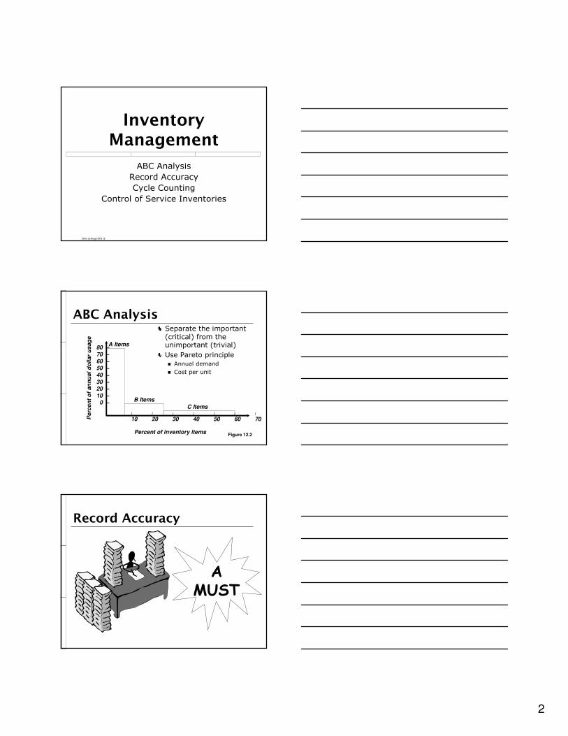
A Items

B ItemsC Items

Per

cent

of a

nnua

l dol

lar

usag

e

80 –70 –60 –50 –40 –30 –20 –10 –

0 –

| | | | | | |

10 20 30 40 50 60 70

Percent of inventory items Figure 12.2

� ��

�

� � � �

3

��

'��-�� %��

.��&�� (��

+�� /��

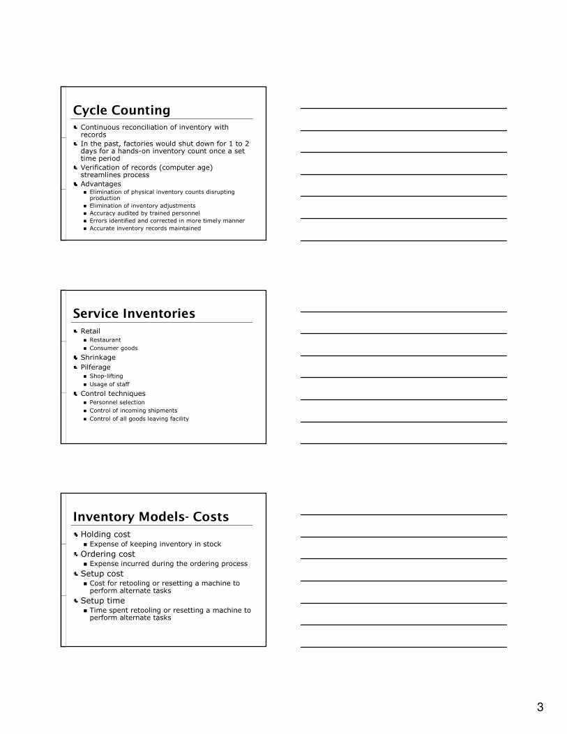
� /�� 0��

� +�� 1 ��

� /��

� +��

� ��

#�� #��

� ��

��

��

� ��%��

� ��

��

� ��

� ��

��

"�� /2��

�� /2��

��

�� 3��

4

��

��

'��4��

'�� "��

��

��

�� !��

��

��

��

��

��

��

�� "��

Figure 12.3

Order quantity = Q (maximum inventory

level)

Inve

ntor

y le

vel

Time

Usage rate Average inventory on hand

Q2

Minimum inventory

5

� �� #��

Objective is to minimize total costs

Table 11.5

Ann

ual c

ost

Order quantity

Curve for total cost of holding

and setup

Holding cost curve

Setup (or order) cost curve

Minimum total cost

Optimal order

quantity

�$ ��

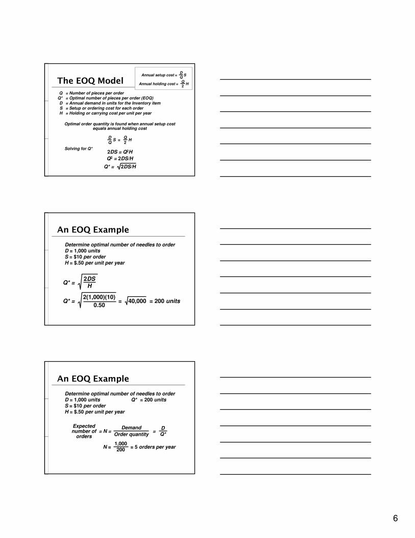
Q = Number of pieces per orderQ* = Optimal number of pieces per order (EOQ)D = Annual demand in units for the Inventory itemS = Setup or ordering cost for each orderH = Holding or carrying cost per unit per year

Annual setup cost = (Number of orders placed per year) x (Setup or order cost per order)

Annual demandNumber of units in each order

Setup or order cost per order

=

= (S)DQ

Annual setup cost = SDQ

�$ ��


Annual holding cost = (Average inventory level) x (Holding cost per unit per year)

Order quantity2

= (Holding cost per unit per year)

= (H)Q2


Annual holding cost = HQ2

6

�$ ��


Optimal order quantity is found when annual setup cost equals annual holding cost


Annual holding cost = HQ2

DQ

S = HQ2

Solving for Q*2DS = Q2HQ2 = 2DS/H

Q* = 2DS/H

�� %��

Determine optimal number of needles to orderD = 1,000 unitsS = $10 per orderH = $.50 per unit per year

Q* =2DS

H

Q* =2(1,000)(10)

0.50= 40,000 = 200 units

�� %��

Determine optimal number of needles to orderD = 1,000 units Q* = 200 unitsS = $10 per orderH = $.50 per unit per year

= N = =Expected number of

orders

DemandOrder quantity

DQ*

N = = 5 orders per year 1,000200

7

�� %��

Determine optimal number of needles to orderD = 1,000 units Q* = 200 unitsS = $10 per order N = 5 orders per yearH = $.50 per unit per year

= T =Expected

time between orders

Number of working days per year

N

T = = 50 days between orders250

5

�� %��

Determine optimal number of needles to orderD = 1,000 units Q* = 200 unitsS = $10 per order N = 5 orders per yearH = $.50 per unit per year T = 50 days

Total annual cost = Setup cost + Holding cost

TC = S + HDQ

Q2

TC = ($10) + ($.50)1,000200

2002

TC = (5)($10) + (100)($.50) = $50 + $50 = $100

��&��

The EOQ model is robustIt works even if all parameters and

assumptions are not metThe total cost curve is relatively flat

in the area of the EOQ

8

� �� '��

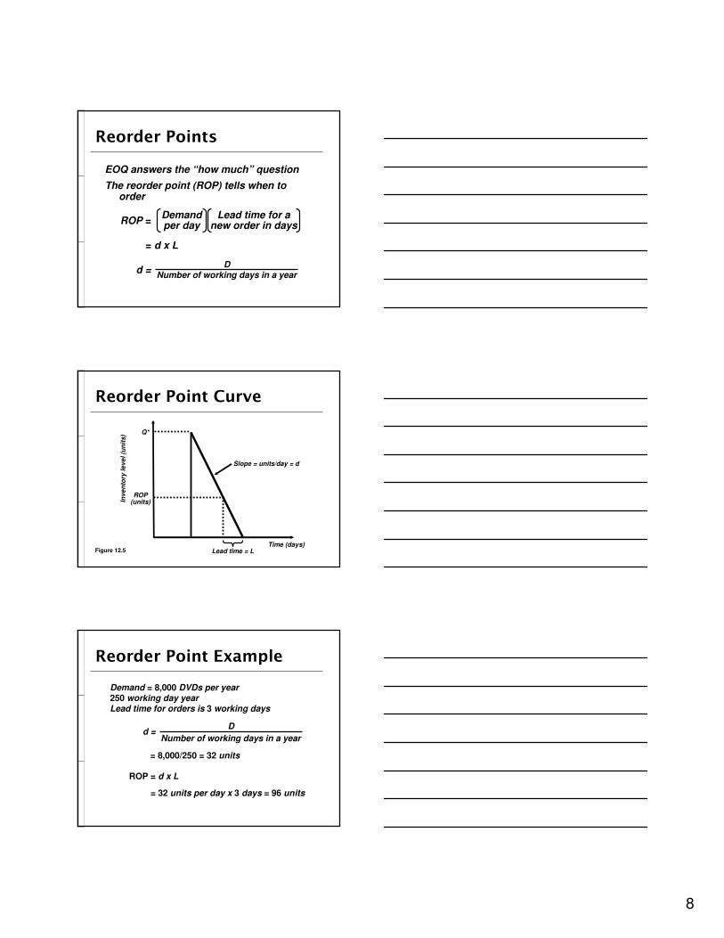
EOQ answers the “how much” questionThe reorder point (ROP) tells when to

order

ROP = Lead time for a new order in days

Demand per day

= d x L

d = DNumber of working days in a year

� �� '��

Q*

ROP (units)In

vent

ory

leve

l (un

its)

Time (days)Figure 12.5 Lead time = L

Slope = units/day = d

� �� '��%��

Demand = 8,000 DVDs per year250 working day yearLead time for orders is 3 working days

ROP = d x L

d = DNumber of working days in a year

= 8,000/250 = 32 units

= 32 units per day x 3 days = 96 units

9

'��

��

��

'��

Inve

ntor

y le

vel

Time

Demand part of cycle with no production

Part of inventory cycle during which production (and usage) is taking place

t

Maximum inventory

Figure 12.6

'��

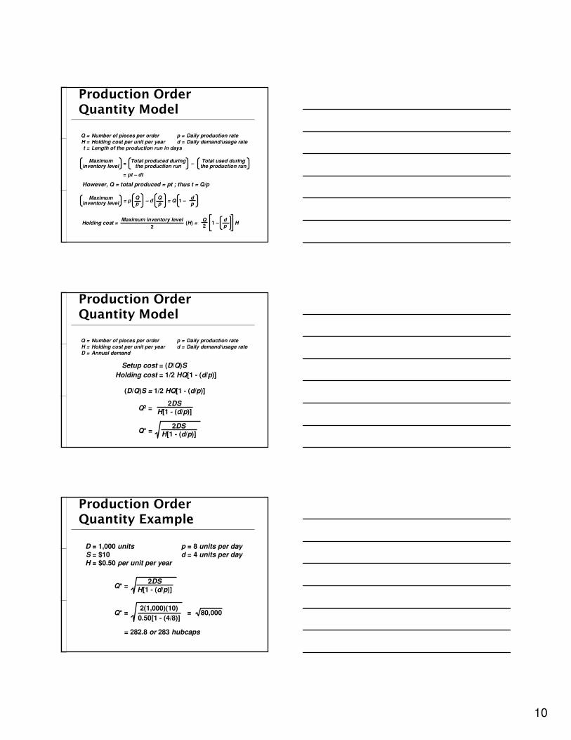
Q = Number of pieces per order p = Daily production rateH = Holding cost per unit per year d = Daily demand/usage ratet = Length of the production run in days

= (Average inventory level) xAnnual inventory holding cost

Holding cost per unit per year

= (Maximum inventory level)/2Annual inventory level

= –Maximum inventory level

Total produced during the production run

Total used during the production run

= pt – dt

10

'��

Q = Number of pieces per order p = Daily production rateH = Holding cost per unit per year d = Daily demand/usage ratet = Length of the production run in days

= –Maximum inventory level

Total produced during the production run

Total used during the production run

= pt – dt

However, Q = total produced = pt ; thus t = Q/p

Maximum inventory level = p – d = Q 1 –Q

pQp

dp

Holding cost = (H) = 1 – H dp

Q2

Maximum inventory level2

'��

Q = Number of pieces per order p = Daily production rateH = Holding cost per unit per year d = Daily demand/usage rateD = Annual demand

Setup cost = (D/Q)SHolding cost = 1/2 HQ[1 - (d/p)]

(D/Q)S = 1/2 HQ[1 - (d/p)]

Q2 =2DS

H[1 - (d/p)]

Q* =2DS

H[1 - (d/p)]

'�� %��

D = 1,000 units p = 8 units per dayS = $10 d = 4 units per dayH = $0.50 per unit per year

Q* =2DS

H[1 - (d/p)]

= 282.8 or 283 hubcaps

Q* = = 80,0002(1,000)(10)

0.50[1 - (4/8)]

11

'��

When annual data are used the equation becomes

Q* =2DS

annual demand rateannual production rateH 1 –

��(��

Reduced prices are often available when larger quantities are purchased

Trade-off is between reduced product cost and increased holding cost

Total cost = Setup cost + Holding cost + Product cost

TC = S + + PDDQ

QH2

��(��

�� 5

��

��

4��

��&�(4��&6(4��7��

4��

8��1��

Table 12.2

A typical quantity discount schedule

12

��(��

1. For each discount, calculate Q*2. If Q* for a discount doesn’t qualify,

choose the smallest possible order size to get the discount

3. Compute the total cost for each Q* or adjusted value from Step 2

4. Select the Q* that gives the lowest total cost

Steps in analyzing a quantity discount

��(��

1,000 2,000

Tota

l cos

t $

0Order quantity

Q* for discount 2 is below the allowable range at point a and must be adjusted upward to 1,000 units at point b

ab

1st price break

2nd price break

Total cost curve for

discount 1

Total cost curve for discount 2

Total cost curve for discount 3

Figure 12.7

��(��%��

Calculate Q* for every discount Q* =2DSIP

Q1* = = 700 cars order2(5,000)(49)

(.2)(5.00)

Q2* = = 714 cars order2(5,000)(49)

(.2)(4.80)

Q3* = = 718 cars order2(5,000)(49)

(.2)(4.75)

13

��(��%��

Calculate Q* for every discount Q* =2DSIP

Q1* = = 700 cars order2(5,000)(49)

(.2)(5.00)

Q2* = = 714 cars order2(5,000)(49)

(.2)(4.80)

Q3* = = 718 cars order2(5,000)(49)

(.2)(4.75)

1,000 — adjusted

2,000 — adjusted

��(��%��

��

��

��

3��

+��

"��

+��

��

+��

��

��7��

��

4��8��1��

Table 12.3

Choose the price and quantity that gives the lowest total cost

Buy 1,000 units at $4.80 per unit

��

��% �' ��

14

��

��/�7�1�� % ��

� 9��

� '��

+�� 8��

4�� "� ��1��

� ��

Inventory Control

Documents

Transcript of Inventory Control