Inventory control as a discrete system control for the fixed-order quantity system

Applied Mathematical Modelling 33 (2009) 4201–4214

Contents lists available at ScienceDirect

Applied Mathematical Modelling

journal homepage: www.elsevier .com/locate /apm

Inventory control as a discrete system control for the fixed-orderquantity system

Konstantin Kostic *

Faculty of Organizational Sciences, University of Belgrade, Jove Ilica 154, 11000 Belgrade, Serbia

a r t i c l e i n f o

Article history:Received 16 December 2007Received in revised form 21 February 2009Accepted 2 March 2009Available online 12 March 2009

Keywords:Inventory controlDiscrete-time systemSimulation-based optimizationEOQ

0307-904X/$ - see front matter � 2009 Elsevier Incdoi:10.1016/j.apm.2009.03.004

* Tel.: +381 11 3241 768.E-mail address: [email protected]

a b s t r a c t

This paper shows how to model a problem to find optimal number of replenishments in thefixed-order quantity system as a basic problem of optimal control of the discrete system.The decision environment is deterministic and the time horizon is finite. A discrete systemconsists of the law of dynamics, control domain and performance criterion. It is primarily asimulation model of the inventory dynamics, but the performance criterion enables variousorder strategies to be compared. The dynamics of state variables depends on the inflow andoutflow rates. This paper explicitly defines flow regulators for the four patterns of theinventory: discrete inflow – continuous/discrete outflow and continuous inflow – contin-uous/discrete outflow. It has been discussed how to use suggested model for variants ofthe fixed-order quantity system as the scenarios of the model. To find the optimal process,the simulation-based optimization is used.

� 2009 Elsevier Inc. All rights reserved.

1. Introduction

As you can see in Axsäter [1], Russell and Taylor [2], Vollmann et al. [3], Chase and Aquilano [4], Barlow [5], Muller [6],Wild [7], even new books dealing with inventory control, describe a classical economic order quantity model and its variantswhen demand rate is constant and known, as a starting point for further understanding of inventory dynamics.

Economic order quantity (also known as the Wilson EOQ Model or simply the EOQ Model) is a model that defines theoptimal quantity to order that minimizes total variable costs required to order and hold inventory. The model was originallydeveloped by Harris [8], though Wilson [9] is credited for his early in-depth analysis of the model. It was a time without easyaffordable computers and the simple useful mathematical models was preferred; see Erlencotter [10] for its history.

A discrete time system is a more natural manner to describe inventory dynamics. Model of discrete system control is botha simulation model of inventory dynamics and an optimization model which can give optimal control according to the de-fined performance criterion.

There are numerous articles using the discrete time system in the deterministic inventory control. These articles addressmainly the lot-sizing problems, beginning with Wagner and Whitin [11], Scarf [12]. In order to find an optimal inventorycontrol for various variants of the dynamic lot-sizing problems, dynamic programming algorithms [13] can be applied. Setchiand Thompson [14] have shown how to apply optimal control theory to management science. There are numerous meta-heuristics algorithms for dynamic lot-sizing problems; see Zoller and Robrade [15] and Jans and Degraeve [16] for anoverview.

The classical EOQ model is considered as a continuous-time approach whereas the lot-sizing problem is considered as adiscrete-time approach. Khmelnitsky and Tzur [17] have analyzed a parallelism of continuous-time and discrete-time

. All rights reserved.

mailto:[email protected]

http://www.sciencedirect.com/science/journal/0307904X

http://www.elsevier.com/locate/apm

4202 K. Kostic / Applied Mathematical Modelling 33 (2009) 4201–4214

production planning problems. They considered the lot-sizing problem ‘‘as the discrete counterpart of the EOQ, since it ismerely a special case of the dynamic demand case”.

The classical EOQ model tackles explicitly the fixed-order quantity system. Lot-sizing models address mainly the periodicreview systems. EOQ model anticipates the saw-tooth pattern as the inventory dynamics. Articles, using dynamic program-ming approach [13], model the dynamics of the stock Xt by using an inflow variable ut as unknown, and outflow variable wt

as deterministic or stochastic one (Xt+1 = Xt + ut � wt, t = 1,2, . . .,T). Both of them subject the model to the optimization meth-od used.

In the simulation-based optimization [18] there is a complete separation between the model that represents the systemand the procedure that is used to solve optimization problems defined within this model. The simulation model can changeand evolve to incorporate additional elements, while the optimization routines remain the same; see Swisher and Hyden[19] and Fu et al. [20] for an overview.

The theoretical foundations for the model of the optimal control of discrete systems can be found in the work of Boltianski[21]. I will interpret it with some additional information.

The principal variable in this approach is discrete time t taking integer values t = 0,1,2, . . .,T, where T is the number ofdays of time horizon.

The state of a system is represented by values of N variables X (Xn, n = 1,2, . . .,N) called ‘‘state variables”. For each variableXn (n = 1,2, . . .,N) there is a co-ordinate of EN Euclid’s space called ‘‘state space”. The state of moving object in time t can berepresented as the point of N-dimensional ‘‘state space”.

Variables, affecting the dynamics of the system and whose values are fixed and known in advance, will be called ‘‘circum-stances variables”. There will be S circumstances variables p, denoted as (ps, s = 1,2 , . . .,S). For each variable ps (s = 1,2 , . . ., S)there is a co-ordinate of ES Euclid’s space called ‘‘circumstances space”. The circumstances of the moving object in time t canbe represented as a point of the S-dimensional ‘‘circumstances space”.

Finally, there will be R variables whose values are unknown and are to be found according to some criteria. These vari-ables will be called ‘‘control variables” and denoted as ur (r = 1 ,2 , . . .,R). For each variable ur (r = 1,2, . . .,R) there is a co-ordi-nate of ER Euclid’s space called ‘‘control space”. A control in time t can be represented as the point of R-dimensional ‘‘controlspace”.

Further in the text, superscripts will be used as labels of co-ordinates of appropriate spaces. Subscripts will denote time atwhich a variable takes a value (current time t or previous time t � 1).

Interrelation among all selected variables can be represented by the law of dynamics:

X0 ¼ known;Xt ¼ f ðXt�1;pt ;utÞ; t ¼ 1;2; . . . ; T

ð1Þ

where

X0 known initial state of the systemf : (f 1, f 2, . . ., f N) N-dimensional vector function with values in EN spaceXt value of N-dimensional vector function at current time tXt�1 value of N-dimensional vector function at previous time t � 1pt value of S-dimensional vector at current time tut value of R-dimensional vector at current time t

A state Xt is obtained as a value of the vector function f (Xt�1,pt,ut) based on the state Xt�1 from the previous time t � 1 andvalues of the circumstances variables pt and control variables ut from the current time t.

An un-empty set Ut 2 (Xt�1,pt) in the space of variables u1,u2, . . .,uR is to be determined for each state point X 2 EN andeach t = 1,2, . . .,T. It is called control domain depending on the value of the state variable Xt�1 from the previous timet � 1 and circumstances variable from the current time t. The control ut can take a value merely from the control domain

ut 2 UtðXt�1; ptÞ; t ¼ 1;2; . . . ; T: ð2Þ

where subscripts denote time at which a variable takes value.Relations of the law of dynamics (1) and control domain (2) determine a discrete controlled object. These relations also

represent the simulation model of the moving object.A series of the circumstances points throughout time horizon p1,p2, . . .,pT is called circumstances of the moving object. A

series of the control points throughout time horizon u1,u2, . . .,uT is called control of the moving object. A series of the statepoints throughout time horizon X1,X2, . . .,XT is called trajectory of the moving object. A logical troika (X,p,u) consisted of tra-jectory (X), circumstances (p) and control (u) is called discrete process.

The success of the control will be measured at each time t (t = 1,2, . . .,T) by defined function f 0(Xt�1,pt,ut). The perfor-mance criterion J is an objective functional that adds values of function f 0 throughout time horizon, i.e.

J ¼ f 0ðX0; p1; u1Þ þ f 0ðX1;p2;u2Þ þ � � � þ f 0ðXt�1;pt ;utÞ ¼XT

t¼1

f 0ðXt�1; pt; utÞ: ð3Þ

K. Kostic / Applied Mathematical Modelling 33 (2009) 4201–4214 4203

2. Inventory flow

Assume that time horizon consists of several (T) time buckets representing days. The demand (D) for period (T) is knownand will be satisfied at constant rate (D/T) or (D/NoO), where NoO is the number of discrete shipments.

The approach of Forester [22] to present system dynamics by stock and flow diagram has proved to be very useful forinventory flow presentation.

A flow of an inventory (Fig. 1) begins with the placing of order YN for certain quantity of items. After that, the ordereditems are in a state of the items on order XN until they are stocked. There is a lead time LT0 between placing an order YN

and getting the item in stock YI. Lead times involve many activities such as order preparation, item production, packaging,transportation, checking on arrival, etc. Items are dispatched from the stock YO according to the demand.

X0; XN0 ¼ known;

XNt ¼ XN

t�1 þ YNt � YI

t ;

0 6 XNt�1 þ YN

t � YIt ;

Xt ¼ Xt�1 þ YIt � YO

t ; t ¼ 1;2; . . . ; T;

0 6 Xt�1 þ YIt � YO

t �Pt

tt¼t�LT 00þ1YI

tt; LT 00 > 0

0; LT 00 ¼ 0

8><>:

9>=>;

ð4Þ

Variable X represents an accumulation of the flow subject, whereas variable Y represents a flow regulator of the input oroutput of the corresponded accumulation. Section 3 of this paper explicitly determines mathematical relations of the flowregulators Y, considering four inventory patterns: discrete inflow – continuous/discrete outflow and continuous inflow –continuous/discrete outflow.

A certain amount of items is ordered whenever the amount on hand X drops below a predetermined level – called thereorder or order point. A reorder level or reorder point is defined as the stock level at which a replenishment order shouldbe placed. When a reorder is made, there must be sufficient stock on hand to cover demand until the order arrives. A reorderlevel can be found by multiplying the average demand D/T by the sum of lead times LT0 + LT00, preceding the moment whenitem shipment is possible. The safety stock will not be considered in this paper, but it can be easily included in the model.

The placement of order YN increases the amount of items on order XN, while the supply procurement of items YI decreasesthis amount. The amount of items on order cannot be negative.

In many inventory control problems there is no delay in receiving and using an order, i.e. replenishment is instantaneous.But a real inventory dynamics must count on a delay between receiving and using an order. A corresponding variable LT00 forthis delay will be included in the law of dynamics.

Replenishment YI increases the on-hand inventory X while depletion YO decreases it. The stock X cannot be negative. Thismeans that certain quantity of stock cannot be shipped in the time t, because of the delay LT00 between receiving and using anorder. This amount is a sum of quantities arrived during LT00 last days.

The two most common approaches to the timing of orders are (i) the fixed-order quantity system, and (ii) the fixed-periodor periodic review system. In the fixed-order quantity system, the same constant amount is ordered every time. Any varia-tion in demand is overcome by changing the time between orders. In the periodic review system, orders are placed at fixedintervals regardless of the size of the stock. Any variation in demand is overcome by changing the size of the order. This pa-per will address the fixed-order quantity system.

This paper defines tree distinguished segments of the inventory model

i. A law of dynamics
� defines a law of dynamics for four inventory patterns considering variants of the inventory inflow and outflow
dynamics on the day by day basis;� according to the type of the inventory outflow, a mathematical relation is given for each type of inventory inflow

depicting the reordering policy that determines the replenishment which occurs when demand falls below adefined level;

ii. A control domain
� main constraint secures non-negativity of the stock;
Fig. 1. Inventory flow.


� there is a possibility to include other necessary constraints limiting stock space, ordered quantity, budget etc.,without corrupting the law of dynamics;

iii. A performance criterion
� given as a functional containing a sum of ordering/setup costs, holding costs and unit costs on the day by day basis.� there is a possibility to restructure the objective function of the performance criterion by fragmentizing costs or
including new approaches for cost calculations without corrupting the law of dynamics.

3. Law of dynamics Xt = f (Xt�1,pt,ut), t = 1,2, . . .,T

Consider only the second part of the described ‘‘inventory flow” from the item arrival YI to the item shipment YO. Let ustake that the first arrival of the item occurs at the beginning of time bucket t = 1. Consequently, there is no need for the leadtime LT0 to be included in the law of dynamics.

There are four patterns depicting inflows and outflows of the stock:

(a) Discrete inflow – continuous outflow.(b) Discrete inflow – discrete outflow.(c) Continuous inflow – continuous outflow.(d) Continuous inflow – discrete outflow.

For mathematical relations of the discrete object the following notation will be used:

t discrete timeT number of days of the time horizon (year)Xt stock at time tX2

t auxiliary variable with value at time t

Y It quantity item received at time t

YOt quantity item dispatched at time t

D item demand for the observed time horizonPR production capacity for the observed time horizonLT0 waiting for appropriate quantity to be delivered/manufacturedLT00 delay between receiving and using ordersNoI number of replenishments/lot sizesNoO number of discrete shipmentsCs setup/order costCh holding/carrying cost per unit for the observed time horizonCu unit cost

3.1. Discrete inflow – continuous outflow

In this pattern, if the lead time LT00 is zero, the on-hand inventory will follow a saw-tooth pattern as shown in Fig. 2. If thelead time LT00 = 5, the on-hand inventory will follow a saw-tooth pattern as shown in Fig. 3. Notice that in the Fig. 3 stock doesnot falls to zero until the end.

Fig. 2. Discrete inflow – continuous outflow.

Fig. 3. Discrete inflow – continuous outflow.


X0 ¼ known;


t ;

YOt ¼

0; t 6 LT 00

D=T; t > LT 00

� �;

YIt ¼

min D=NoI; D�Pt�1

tt¼1YI

tt

� �; Xt�1 < ð1þ LT 00Þ � D=T

0; otherwise

8><>:

9>=>;;


t �Pt

tt¼t�LT 00þ1YI

tt; LT 00 > 0

0; LT 00 ¼ 0

8><>:

9>=>;;

t ¼ 1;2; . . . ; T:

ð5Þ

As demand rate is constant, outflow of items will be D/T per day until entire demand is satisfied. If shortages are not al-lowed, the quantity D/NoI is assumed to arrive whenever the quantity on hand falls below a daily demand above the quantityneeded in LT00 days (if the lead time LT00 is greater than zero). Items will be ordered until demand is satisfied. Replenishmentwill occur in NoI equal quantities D/NoI.

The expression ‘‘minðD=NoI; D�Pt�1

tt¼1YIttÞ” permits NoI to be non-integer in order to enable simulation of the solutions

obtained by the EOQ model. In such instances the first NoI � 1 orders will be equal quantities whereas the last one willbe supplement to the quantity demanded D. The non-equation in the model assures non-negativity of the stock by takingin account that arrived quantity YI

t cannot be used before a preparation for the depleting.

3.2. Discrete inflow – discrete outflow

In this pattern, if the lead time LT00 is greater than zero, the on-hand inventory will follow a saw-tooth pattern as shown inFig. 4.

X0 ¼ known;


t ;

YOt ¼

D=NoO; ð1þ LT 00 þ intðt=intðT=NoOÞ � kÞ � intðT=NoOÞ ¼ tÞ \ ðPt�1

tt¼1YO

tt < DÞ

0; otherwise

8><>:

9>=>;;

k ¼ 1; t P 1þ LT 00 P intðT=NoOÞ0; otherwise

( );

YIt ¼

min D=NoI;D�Pt�1

tt¼1YI

tt

� �; ð1þ intðt=intðT=NoIÞÞ � intðT=NoIÞ ¼ tÞ \

Pt�1

tt¼1YI

tt < D� �

0; otherwise

8><>:

9>=>;;


t �Pt

tt¼t�LT 00þ1YI

tt; LT 00 > 0

0; LT 00 ¼ 0

8><>:

9>=>;;

t ¼ 1;2; . . . ; T:

ð6Þ

Function ‘‘int” gives an integer of its argument.As demand rate is constant, outflow of items (D/NoO) will occur at defined time in NoO equal quantities until entire de-

mand is satisfied. If shortages are not allowed, the schedule of NoI discrete arrivals should secure enough quantity in thestock for the smooth discrete shipment. Items will be ordered until demand is satisfied. Replenishment will occur in NoI

equal quantities Q.As in the previous pattern, the expression ‘‘minðD=NoI; D�

Pt�1tt¼1YI

ttÞ” reflects the fact that the total replenishment has toequals total demand D. It permits NoI to be non-integer in order to enable simulation of the solutions obtained by the PROQ

Fig. 4. Discrete inflow – discrete outflow.


model. In such instances the first NoI � 1 batches will be equal quantities whereas the last one will be supplement to thequantity demanded D. The non-equation in the model assures non-negativity of the stock by taking in account that arrivedquantity YI

t cannot be used before preparation for the depleting.

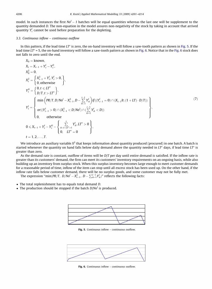
3.3. Continuous inflow – continuous outflow

In this pattern, if the lead time LT00 is zero, the on-hand inventory will follow a saw-tooth pattern as shown in Fig. 5. If thelead time LT00 = 5, the on-hand inventory will follow a saw-tooth pattern as shown in Fig. 6. Notice that in the Fig. 6 stock doesnot falls to zero until the end.

X0 ¼ known;


t ;

X20 ¼ 0;

X2t ¼

X2t�1 þ YI

t; YIt > 0;

0;otherwise

( );

YOt ¼

0; t 6 LT 00

D=T; t > LT 00

� �;

YIt ¼

min PR=T;D=NoI � X2t�1;D�

Pt�1

tt¼1YI

tt

� �if ððYI

t�1 ¼ 0Þ \ ðXt�1lt; ð1þ LTÞ � D=TÞÞ

orððYIt�1 > 0Þ \ ðX2

t�1 < D=NoIÞ \ ðPt�1

tt¼1YI

tt < DÞÞ

0; otherwise

8>>>>><>>>>>:

9>>>>>=>>>>>;;


t �Pt

tt¼t�LT 00þ1YI

tt; LT 00 > 0

0; LT 00 ¼ 0

8><>:

9>=>;;

t ¼ 1;2; . . . ; T:

ð7Þ

We introduce an auxiliary variable X2 that keeps information about quantity produced (procured) in one batch. A batch isstarted whenever the quantity on hand falls below daily demand above the quantity needed in LT00 days, if lead time LT00 isgreater than zero.

As the demand rate is constant, outflow of items will be D/T per day until entire demand is satisfied. If the inflow rate isgreater than its customers’ demand, the firm can meet its customers’ inventory requirements on an ongoing basis, while alsobuilding up an inventory from surplus stock. When this surplus inventory becomes large enough to meet customer demandsfor a reasonable period of time, inflow of the item can stop until all excess stock has been used up. On the other hand, if theinflow rate falls below customer demand, there will be no surplus goods, and some customer may not be fully met.

The expression ‘‘minðPR=T; D=NoI � X2t�1; D�

Pt�1tt¼1YI

ttÞ” reflects the following facts:

� The total replenishment has to equals total demand D.� The production should be stopped if the batch D/NoI is produced.

Fig. 5. Continuous inflow – continuous outflow.

Fig. 6. Continuous inflow – continuous outflow.


� A day production rate PR/T is a uniform fraction of the annual production rate PR; if the total demand D or the batch D/NoI

is met, it is not necessary to use a full day production rate PR/T.

The non-equation in the model assures non-negativity of the stock by taking in account that arrived quantity YIt cannot be

used before a preparation for the depleting.

3.4. Continuous inflow – discrete outflow

In this pattern there must be a time delay which is necessary for the manufacturing (accumulation) of the quantity ofitems needed for at least one discrete shipment. It means that the lead time LT0 has to be greater than zero. If shortagesare not allowed, the manufacturing of the lot size Q is assumed to start at the right time which is long enough for the accu-mulation of the needed quantity D/NoO. Let us take that the production run starts at the beginning of the time bucket t = 1.Taking into account the lead time LT00 between receiving and using items, the first discrete shipment occurs after LT0 + LT00

days. Therefore, if the sum of lead times LT0 + LT00 is greater than zero, the on-hand inventory will follow a saw-tooth patternas shown in Fig. 7.

As demand rate is constant, outflow of items will occur at the defined time in equal quantities until all demand is satis-fied. If the inflow rate is greater than the customers’ demand, the firm can meet its customers’ inventory requirements on anongoing basis, while also building up an inventory from surplus stock. When this surplus inventory becomes large enough tomeet customer’s demand for a reasonable period of time, inflow of the item can stop until all excess stock has been used up.On the other hand, if the inflow rate falls below customer’s demand, there will be no surplus goods, and some customer maynot be fully met.

As in the previous pattern, an auxiliary variable X2 keeps information about the quantity manufactured in one batch. Abatch is started whenever the quantity on hand falls below the quantity needed to satisfy demand until new discrete ship-ment is prepared.

X0 ¼ known;


t ;

X20 ¼ 0;

X2t ¼

X2t�1 þ YI

t ;YIt > 0

0;otherwise

( );

YOt ¼

D=NoO; if ð1þ LT 0 þ LT 00 þ intðt=intðT=NoOÞ � kÞ � intðT=NoOÞ ¼ tÞ \Pt�1

tt¼1YO

tt < D� �

0; otherwise

8><>:

9>=>;;

k ¼ 1; t P 1þ LT 0 þ LT 00 P intðT=NoOÞ0; otherwise

( );

YIt ¼

min PR=T;D�Pt�1

tt¼1YI

tt

� �; if ðYI

t�1 > 0Þ \ ðX2t�1 < D=NoIÞ \

Pt�1

tt¼1YI

tt < D� �

orðYIt�1 ¼ 0Þ \

Pt�1

tt¼1YI

tt < D� �

\ ðXt�1 < ð1þ intðNoO � ðLT 0 þ LT 00Þ=TÞÞ � D=NoOÞ

0; otherwise

8>>>>><>>>>>:

9>>>>>=>>>>>;;


t �Pt

tt¼t�LT 00þ1YI

tt; LT 00 > 0

0; LT 00 ¼ 0

8><>:

9>=>;;

t ¼ 1;2; . . . ; T:

ð8Þ

Function ‘‘int” gives an integer of its argument.

Fig. 7. Continuous inflow – discrete outflow.


4. Control domain ut ‰ U(Xt�1,pt), t = 1,2, . . .,T

The main constraint is that a stock cannot be negative.


t �Pt

tt¼t�LT 00þ1YI

tt; LT 00 > 0

0; LT 00 ¼ 0

8><>:

9>=>;; t ¼ 1;2; . . . ; T: ð9Þ

Additional constraints can be imposed according to the real decision environment. As the production rate per day (PR) canbe a constraint, so can the suppliers’ limitation on ordered quantity. Because of resource limitations, one can include con-straints on storage space, investment in stock, machine availability, delivery capacity and frequency, etc. There can be a lim-itation on time that item spends in warehouse.

All existed constraints define a set U(Xt�1,pt), t = 1,2, . . .,T, i.e. control domain of the discrete object. The control variable ut

can take values merely from the control domain, ut 2 U(Xt�1,pt), t = 1,2, . . .,T.

5. Performance criterion J ¼ +Tt¼1f 0ðXt�1;pt ;utÞ

Reasons for holding stock items are (i) to enable production processes to operate smoothly and efficiently, (ii) to takeadvantage of quantity discounts, (iii) to protect against possible shortages in the future, (iv) to absorb seasonal fluctuationsin demand and supply, (v) to protect against inflation and price changes.

The goal to ensure that anticipated demand be met is achieved by keeping stock nonnegative. However, the primary pur-pose of inventory control is to ensure that the right amount of the right item is ordered at the right time, according to knowndemand, existed constraints and the objective to minimize total cost, where cost is given by the equation

cost ¼ ordering-costþ holding-costþ purchase-cost

5.1. Ordering (or setup) cost

Ordering cost includes costs arising from the preparation and dispatch of the order, checking of the goods on delivery, andother clerical support activities. It can be constant (EOQ model) or variable throughout time horizon, depending (IncreasingDelivery Costs – a variation of the Discount model), or not on the ordered quantity. Ordering (or setup) cost per order (setup)Cs is greater than zero only in time t when order arrives in the stock or when the batch is started.

5.2. Holding (or carrying) cost

The cost of holding one unit of an item in stock per day (for instance $20/T a unit per day or as a percentage of the unitcost of the item divided by T, where T is the number of days of time horizon). Holding costs include interest on the capitaltide up in stock, insurance, storage charges (rent, lighting, heating, refrigeration, etc.), deterioration and obsolescence ofstock. It can be constant (EOQ model) or variable throughout time horizon, depending or not of the quantity carried in inven-tory. Holding (carrying) cost per one unit Ch per day multiplies a day average inventory. If we retain a classical inventorycontrol model approach, a day average (dav) inventory can be counted as:

Discrete inf low� Continuous outflow;

dav ¼ Xt�1 þ YIt � YO

t =2; t ¼ 1;2; . . . ; T;

Discrete inf low� Discrete outflow;

dav ¼ Xt�1 þ YIt � YO

t ; t ¼ 1;2; . . . ; T;

Continuous inf low� Continuous outflow;

dav ¼ Xt�1 þ ðYIt � YO

t Þ=2 ; t ¼ 1;2; . . . ; T;

Continuous inf low� Discrete outflow;

dav ¼ Xt�1 þ YIt=2� YO

t ; t ¼ 1;2; . . . ; T:

ð10Þ

5.3. Purchase (unit) cost

Purchase (unit) cost is the price charged by suppliers for one unit of the item. It can be constant (EOQ model) or variablethroughout time horizon, depending (Quantity Discount model) or not on the ordered quantity. Purchase (unit) cost Cu mul-tiplies quantity purchased (manufactured) in time t.


In the case of the discrete inflow, the general pattern of the performance criterion is

J ¼XT

t¼1

Cs �1; YI

t > 0

0; YIt ¼ 0

( )þ Ch � davðYI

tÞ þ Cu � YIt

" #; ð11aÞ

that should be minimized.In the case of the continuous inflow, the general pattern of the performance criterion is

J ¼XT

t¼1

Cs �1; YI

t > 0 \ YIt�1 ¼ 0

0; YIt ¼ 0


tÞ þ Cu � YIt

" #; ð11bÞ

that should be minimized.It is obvious that the value of performance criterion depends on the inflow dynamics YI

t . The function of the performancecriterion can contain additional information according to the real decision environment.

6. Circumstances pt and control ut variables

All model included factors can be taken as variables: some of them as dependent and other as independent. Variableswith in advance known values throughout time horizon are circumstances of discrete system (denoted as ps

t , s = 1,2, . . .,S).The principal characteristic of the circumstances variables determining the law of dynamics when demand rate is constantand known, is that they are constant throughout time horizon for each t = 1,2, . . .,T (p1 = p2 = . . .=pT). They are:

D item demand for the observed time horizonPR production capacity for the observed time horizonLT0 waiting for appropriate quantityLT00 delay between receiving and using orders

On the other hand, the circumstances variables determining elements for the performance criterion can be either con-stant or variable throughout time horizon, independent or dependent on the inflow. They are:

Cu or Cu(Y It) unit price

Ch or Ch(Y It) unit holding cost per day

Cs or Cs(YIt) ordering/setup cost per order etc.

Existed dependences are usually defined as table functions.As for the control domain, included circumstances variables can be also either constant or variable throughout time hori-

zon. It depends on the nature of the decision environment parameter represented by the circumstances variables.Values of some model variables are unknown in advance and should be determined according to the performance crite-

rion and defined constraints. These variables are considered as control variables (denoted as urt , r= 1,2, . . .,R). There is just one

control variable (R = 1) for one inventory item in the case of the inventory control when demand rate is constant and known.It will be a number of replenishments or manufacturing setups NoI.

The control variable ut represents an unknown number of replenishments or manufacturing setups NoI, (NoI = ut,t = 1,2, . . .,T). Because NoI is constant throughout time horizon, there is just one value of NoI which should be found. Conse-quently, equation u1 = u2 = u3 = . . . = uT is to be included in the model as a constraint of the control domain.

The second fact is that the number of replenishments or manufacturing setups NoI can be merely an integer between 1and T. It results from the nature of the fixed-order politics and it should be included into control domain relations.

7. Problem of the optimal control of discrete system

The law of dynamics, control domain and performance criterion in the basic problem of optimal control, contain onlystate variables Xt�1 from the previous time t � 1, circumstances pt and control ut variables from the current time t [21].

The initial state X0 is known. There is a set Mt in the phase space EN for each t = 1,2, . . .,T.Find an admissible control u1,u2, . . .,uT for the discrete controlled object

Xt ¼ f ðXt�1;pt;utÞ;ut 2 UtðXt�1;ptÞ;

ð12Þ

transferring the controlled object from the initial state X0 into the set of finite phase states XT 2MT for the given time T,according to the circumstances variables p1,p2, . . .,pT and obeying the condition Xt 2Mt for each t = 1,2, . . .,T. The objectivefunctional

J ¼XT

t¼1

f 0ðXt�1;pt ;utÞ; ð13Þ

should get the minimum value for the chosen discrete process (Xt�1,pt,ut, t = 1,2, . . .,T).


There is a finite number of discrete processes (Xt�1,pt,ut) which satisfy imposed conditions. The problem is how to chooseone giving minimum to the performance criterion J.

Since the control variable represents a number of replenishments or manufacturing setups NoI, there are T (T 6 365) pos-sible values of ‘‘NoI”. As there are ‘‘just a few discrete process-candidates”, it makes a sense to check all of them. The ‘‘totalsearch” technique checks each discrete process with a control point from the control domain ut 2 UtðXt�1; ptÞ.

The general steps to solve the problem of the optimal control of discrete system by using total search technique are:

1. Determine a search domain as minimum and maximum value for each co-ordinate of the R-dimensional control space.2. Select a new control u1 = u2 = . . . = uT from the search domain.3. Check if the control satisfies constraints of the control domain, i.e. if ut 2 U(Xt�1,pt), t = 1,2, . . .,T4. If the selected discrete process (Xt�1, pt,ut) is not admissible return to the step 2.5. Compute the value of the performance criterion J for the selected discrete process (Xt�1, pt,ut).6. If the value of the performance criterion is less than previous one, remember discrete process (Xt�1,pt,ut) and the value of

the performance criterion J.7. If there is new control in the search domain go to the step 2, else finish the searching process.

The optimal discrete process is the last one remembered, giving minimum to the performance criterion J.

8. Discussion

Discrete controlled object (12) is the simulation model of inventory dynamics representing stock in discrete time pointsof the time horizon, for example in days. It can be easily developed in a spreadsheet in order to present obviously realisticdynamics of a stock by tables and charts on the day by day basis. Constraints of the control domain ut 2 U(Xt�1,pt),t = 1,2, . . .,T, secure dynamics of the stock to be really admissible. Also, there is a performance criterion (13) as the measureof control quality. The searching algorithms compare the values of the performance criterion for various admissible discreteprocesses (control points) and choose the best process examined. The post-optimal analysis can be performed as a ‘‘Whatif. . .” analysis.

The discrete system model is developed in the VBA (Visual Basic for Applications) in order to demonstrate its usefulness.The application with the user’s instructions can be downloaded from the address: http://uprsys.fon.rs/uprsis/dynamics.xls[23].

The classical EOQ model and its variants, give just the value of total inventory costs TC, and reorder quantity Q. Thedynamics of stock is in advance assumed (a row of identical triangles), but the obtained solution is often dissonant withthe reality.

The classical deterministic inventory models with known and constant demand rate can be considered as special sub-cases (scenarios) of the inventory model as the discrete system control.

8.1. Economic order quantity (EOQ) model

The pattern of this model is discrete inflow – continuous outflow. Annual demand D is known and daily demand D/T isconstant. Ordering cost Cs, holding cost per unit per year (per day) Ch and unit cost Cu are constant and independent. Theoptimal order quantity is obtained as D/NoI where the number of replenishments NoI is to be found, so that the performancecriterion J gets a minimum value. The EOQ model provides a real number grater then zero as the number of replenishmentsNoI.

By comparing the total inventory cost TC, obtained by the EOQ model, and the minimum value of the performance crite-rion J, obtained by the discrete system control, we conclude that they are equal only if the EOQ model gives a number ofreplenishments NoI as an integer (Table 1). In other cases, the minimum value of the performance criterion J is obviouslya better measure of the total inventory cost.

The Table 2 depicts a situation when the EOQ model gives a fractured number as a number of replenishments NoI. A frac-tured number of replenishments is in collision with the premise that all orders are equal (fixed-order quantity system). Fur-thermore, order cost Cs cannot be multiplied by a fractured number as the EOQ model does it. Therefore, it is necessary to

Table 1Example when EOQ and total search give equal results.

Problem EOQ model found Total search found

T = 360 days EOQ = 400 units per order YIt ¼ 400 units per order

D = 12,000 per year TC = $303.000 J = $303.000Cs = $50 per order NoI = 30 Ut = 30Ch = $7.5 per unit per yearCu = $25 per unit

http://uprsys.fon.rs/uprsis/dynamics.xls

Table 2Example when EOQ and total search give different results.

Problem EOQ model found Total search found

T = 360 days EOQ = 2666.53 units per order YIt ¼ 2400 units per order

D = 12,000 per year TC = $319,999 J = S320110Cs = $2222 per order NoI = 4.5 Ut = 5Ch = $7.5 per unit per yearCu = $25 per unit

Solution analysisFor NoI = 4.5 For NoI = 4 For NoI = 5EOQ = D/NoI = 12,000/4.5 = 2666.67 EOQ = D/NoI = 12,000/4 = 3000 EOQ = D/NoI = 12,000/5 = 2400TC = 4.5 � 2222 + 25 � 12,000 + 7.5�2666.67/

2 = 319,999.01TC = 4 � 2222 + 25 � 12,000 + 7.5 � 3000/2=32,0128

TC = 5 � 2222 + 25�12,000 + 7.5 � 2400/2 = 320,110


check neighboring integers (4) and (5) as possible numbers of replenishments and to choose one which gives smaller totalcosts TC. As a conclusion, the discrete time system gives a better solution of the inventory control than EOQ model in thefixed-order system with the finite time horizon. This remark holds in the next pattern as well.

8.2. Production order quantity (PROQ) model

The pattern of this model is continuous inflow – continuous outflow. Annual demand D is known and daily demand D/T isconstant. Annual production rate PR is known and daily production rate PR/T is constant. Setup cost Cs, holding cost per unitper year (per day) Ch and unit cost Cu are constant and independent. The optimal lot size is obtained as D/NoI where thenumber of setups NoI is to be found so that the performance criterion J gets a minimum value. There is T possible integervalues for the number of setups NoI.

By comparing the total inventory cost TC, obtained by the PROQ model, and the minimum value of the performance cri-terion J, obtained by the discrete system control, we conclude that they are equal only if the PROQ model gives a number ofsetups NoI as an integer (Table 3). In other cases, the minimum value of the performance criterion J is obviously a better mea-sure of the total inventory cost.

The Table 4 depicts a situation when the PROQ model gives a fractured number as a number of setups NoI. A fracturednumber of setups is in collision with the premise that all orders are equal (fixed-order quantity system). Furthermore, set-up-cost Cs cannot be multiplied by a fractured number as the PROQ model does it. Therefore, it is necessary to check

Table 3Example when PROQ and total search give equal results.

Problem PROQ model found Total search found

T = 360 days PROQ = 1000 units per order YIt ¼ 1000 units per order

D = 2000 per year TC = $14,766.67 NoI = 2 J = $14766.67PR = 3000 per year Ut = 2Cs = $16.67 per orderCh = $0.2 per unit per yearCu = $7.35 per unit

Table 4Example when PROQ and total search give different results.

Problem PROQ model found Total search found

T = 360 days PROQ = 1549.19 unit per order YIt ¼ 2000 units per order

D = 2000 per year TC = $14,803.28 J = $14,806.67PR = 3000 per year No = 1.291 Ut = 1Cs = $40 per orderCh = $0.2 per unit per yearCu = $7.35 per unit

Solution analysisFor NoI = 1.291 For No = 1 For NoI =2PROQ = D/NoI =

2000/1.291 = 1549.19PROQ = D/NoI = 2000/1 = 2000 PROQ = D/NoI = 2000/5 = 1000

TC = 1.291 � 40 + 7.35 � 2000 +0.2�1549.19�(1 � 2000/3000)/2 = 14803.28

TC = 1 � 40 + 7.35 � 2000 + 0.2 �2000 � (1 � 2000/3000)/2 = 14806.67

TC = 2�40 + 7.35 � 2000 + 0.2 � 1000 �(1 � 2000/3000)/2 = 14813.33


neighboring integers (1) and (2) as possible numbers of replenishments and to choose one which gives smaller total costs TC.As a conclusion, the discrete time system gives a better solution of the inventory control than PROQ model in the fixed-ordersystem with the finite time horizon. This remark holds in the next patterns as well.

8.3. Quantity discount model

The pattern of this model is discrete inflow – continuous outflow. Annual demand D is known and daily demand D/Tis constant. Ordering cost Cs and holding cost per unit per year (per day) Ch are constant and independent. Unit costCu(D/NoI) depends upon the size of the order. This dependence is given as a table function and it is constant throughoutthe time horizon. The optimal order quantity is obtained as D/NoI where the number of replenishments NoI is to be foundso that the performance criterion J gets a minimum value. There is T possible integer values for the number of replenish-ments NoI.

8.4. Increasing delivery costs – a variation of the discount model

The pattern of this model is discrete inflow – continuous outflow. Annual demand D is known and daily demand D/T isconstant. Holding cost per unit per year (per day) Ch and unit cost Cu are constant and independent. Ordering cost Cs(NoI)depends upon the number of deliveries required. This dependence is given as a table function that is constant throughoutthe time horizon. The optimal order quantity is obtained as D/NoI where the number of replenishments NoI is to be foundso that the performance criterion J gets a minimum value. There is T possible integer values for the number of replenish-ments NoI.

8.5. Inventory models with planned shortage

Inventory models with planned shortages handle stock-outs by back-ordering. A back-order policy allows planned short-ages to occur, with customer demand being met after an order has been placed. A back-order policy assumes that customersare willing to wait for delivery, but it does not mean that stock is negative: the stock is zero and back-order list is rising untilit is satisfied. Model can contain a flow of back-orders with inflow representing mounting of unsatisfied demand and outflowrepresenting customers demand meting.

In the case of the planed shortages, a new state variable Xsh should be introduced for each item. If there is no item in thestock, the inflow YshI

t will be greater than zero and equal to the daily shortage. When the next order arrives it will contain alsothe amount needed for the cumulative back-order to be fulfilled. It means that YshO

t will be equal to cumulative of back-or-ders Xsh

t�1 at the moment of the order arrival.

Xsh0 ¼ known;

Xsht ¼ Xsh

t�1 þ YshIt � YshO

t ;

0 6 Xsht�1 þ YshI

t � YshOt ;

YshIt ¼

Q sh; YOt > Xt�1 þ YI

t

0; otherwise

( );

YshOt ¼ Xt�1; ðYI

t > 0Þ \ ðXsht�1 > 0Þ

0; otherwise

( );

t ¼ 1;2; . . . ; T;

ð14Þ

where

Qsh shortageXsh cumulative of back – ordersYshI unfulfilled ordersYshO satisfying back – ordersX stock of itemYI item arrivalYO item dispatching

As for the performance criterion, the statement about a shortage cost should be included. A shortage cost (penalty) perunit per day ‘‘B” multiplies a daily back-order Xsh

t . Consequently, the objective functional J is broaden as

J ¼XT

t¼1

Cs ��

1; YIt > 00; YI

t ¼ 0�þ Ch � davðYI

tÞ þ B � ðXsht�1 þ YshI

t =2� YshOt Þ þ Cu � YI

t

� �; ð15aÞ


for the case of the continuous outflow, or

J ¼XT

t¼1

Cs �1; YI

t > 0

0; YIt ¼ 0


tÞ þ B � ðXsht�1 þ YshI

t � YshOt Þ þ Cu � YI

t

" #; ð15bÞ

for the case of the discrete outflow.The objective functional should be minimized.In order to use this part of model, it is necessary to slightly modify previously described model in the part concerning the

inflow politics YIt . The arrived quantity should contain also a back-ordered quantity. Also, there is a need to consider what

will happen with the back-order at the terminate date of the time horizon: will it be undelivered or delivered in an additionaltime. This decision affects the performance criterion.

9. Conclusion

The model of the inventory control as the discrete system control can be successfully used as a general dynamic model foranalyzing inventory dynamics over a finite time horizon in the case of the fixed-order quantity system. When developed in aspreadsheet (tables and charts) it is a great tool for both academics and professionals to better understand dynamics of theinventory on the day by day basis.

This model clearly distinguish the law of dynamics, control domain and performance criterion. It is very useful when oneanalyzes the business decision environment: firstly, establish the law of dynamics; secondly, determine the control domain;thirdly, define an objective function which will be incorporated into the performance criterion. After that, one can perform‘‘what if” analyzes or a meta-heuristics search in order to find the optimal solution which can be simulated and analyzed.

The proposed model explicitly defines mathematical relations of the inventory inflow YI and outflow YO for each of pos-sible inventory patterns: discrete inflow – continuous/discrete outflow and continuous inflow – continuous/discrete outflow.The mathematical relation for the inventory inflow YI reflects inventory policy to replenish items whenever stock falls belowdefined level. The mathematical relation for the inventory outflow YO reflects the model assumption that the demand isknown and at a constant rate (continuous or discrete).

The main constraint for the control domain secures non-negativity of the stock. Additional constraint can be easily addedin order to describe resource scarceness, without corrupting the law of dynamics.

Also, the objective function of the performance criterion J can be modified, without corrupting the law of dynamics. Mod-ifications of the objective function can include costs divergences or new costs introduction. Various inventory decision envi-ronments can be described by combining the nature of circumstances variables: constant or variable throughout timehorizon, independent or dependent on each other.

A set of classical inventory models is obtained by modifying EOQ model: Production order quantity model, Quantity dis-count model, Inventory model with planned shortages, etc., with specific techniques for solving each of their problems. All ofthem can be presented by the discrete-time system as the scenarios of the special cases of the inventory dynamics. Workingwith the model of discrete system control, the limitations of the classical model are overcome.

The model and searching method are separated. The various searching methods can be used over the model, The pre-sented algorithm of the ‘‘total search” finds an optimal discrete process (X,p,u) very fast because there are ‘‘just a few dis-crete process-candidates”. If the model is developed in a spreadsheet, there is no advantage of the simplicity of the classicalEOQ model.

Moreover, problem of optimal control of discrete system is well structured and there are meta-heuristics algorithms withprovably good run times and with provably good or optimal solution quality. As the search methods (meta-heuristics algo-rithms) are rapidly developing and computers are faster than ever (and will be), the time has come to use simulation-basedtechniques of the optimal control of discrete system in respect to inventory control both in the education and in professionalwork.

References

[1] S. Axsäter, Inventory Control (International Series in Operations Research & Management Science), Springer Science + Business Media, New York, 2006.pp. 51–60.

[2] R. Russell, B. Taylor, Operations Management: Quality and Competitiveness in a Global Environment, Wiley, New York, 2006. pp. 529–552.[3] T. Vollmann, W. Berry, D. Whybark, R. Jacobs, T. Vollmann, W. Berry, Manufacturing Planning and Control Systems for Supply Chain Management: The

Definitive Guide for Professionals, McGseries Hill, New York, 2005. pp. 118–146.[4] R. Chase, N. Aquilano, Operations Management for Competitive Advantage, IRWIN, New York, 2004. pp. 542–560.[5] J. Barlow, Excel Models for Business and Operations Management, Wiley, New York, 2003. pp. 244–258.[6] M. Muller, Essentials of Inventory Management, AMACOM, New York, 2003. pp. 115–129.[7] T. Wild, Best Practice in Inventory Management, Elsevier Science, London, 2002. pp. 112–148.[8] F.W. Harris, How many parts to make at once, factory, Mag. Manage. 10 (2) (1915) 135–136. 152.[9] R.H. Wilson, A scientific routine for stock control, Harvard Business Rev. 13 (1934) 116–128.

[10] D. Erlencotter, An early classic misplaced: Ford W. Harris’s economic order quantity model of 1915, Manage. Sci. 35 (7) (1989).[11] H.M. Wagner, T. Whitin, Dynamic version of the economic lot size model, Manage. Sci. 5 (1) (1958) 89–96.[12] H. Scarf, The optimality of (s; S) policies in the dynamic inventory problem, in: Arrow, Karlin, Patrick (Eds.), Proceedings of the First Stanford

Symposium ‘‘Mathematical Methods in the Social Sciences, 1959”, 1959.[13] D.P. Bertsekas, Dynamic Programming – Deterministic and Stochastic Models, Prentice-Hall, Englewood Cliffs, New Jersey, 1987.


[14] S. Setchi, G.L. Thompson, Optimal Control Theory: Applications to Management Science, Martinus Nijhoff, Boston, MA, 1981.[15] K. Zoller, A. Robrade, Efficient heuristics for dynamic lot sizing, Inter. J. Prod. Res. 26 (1988) 249–265.[16] R. Jans, Z. Degraeve, Meta-heuristics for dynamic lot sizing: a review and comparison of solution approaches, Eur. J. Oper. Res. 177 (3) (2007) 1855–

1875.[17] E. Khmelnitsky, M. Tzur, Parallelism of continuous-and discrete-time production planning problems, IIE Trans. 36 (2004) 611–628.[18] F. Glover, J.P. Kelly, M. Laguna, New advances and applications of combining simulation and optimization, in: J.M. Charnes, D.J. Morrice, D.T. Brunner,

J.J. Swain (Eds.), Proceedings of the 1996 Winter Simulation Conference, 1996, pp. 144–152.[19] J.R. Swisher, P.D. Hyden, A survey of simulation optimization techniques and procedures, in: J.A. Joines, R.R. Barton, K. Kang, P.A. Fishwick (Eds.),

Proceedings of the 2000 Winter Simulation Conference, 2000, pp. 119–128.[20] M.C. Fu, F.W. Glover, J. April, Simulation optimization: a review, new developments, and applications, in: M.E. Kuhl, N.M. Steiger, F.B. Armstrong, J.A.

Joines (Eds.), Proceedings of the 2005 Winter Simulation Conference, 2005.[21] V.G. Boltianski, Optimal Control of Discrete Systems, Wiley, New York, 1978. pp. 9–38.[22] J.W. Forester, Principles of Systems, Pegasus Communications, Boston, 1968. pp. 5–30.[23] K. Kostic, Dynamics, Application in VBA for Excel. <http://uprsys.fon.rs/uprsis/dynamics.xls>, 2007.

http://uprsys.fon.rs/uprsis/dynamics.xls

Inventory control as a discrete system control for the fixed-order quantity system

Documents

Transcript of Inventory control as a discrete system control for the fixed-order quantity system