Control system synthesis strategies

9 = stream function 7 = nondimensional time

Subscripts

S = steady state conditions W m

= conditions at the wall = conditions far away from the wall

Superscript

* = physical variables

LITERATURE CITED

Acrivos, A,, M. J. Shah, and E. E. Petersen, “Momentum and Heat Transfer

in Laminar Boundary Layer Flows of Non-Newtonian Fluids Past Ex- ternal Surfaces,” AIChE ./., 6,312 (1960).

Gorla, R. S. R., “Unsteady Thermal Boundary Layers in Non-Newtonian Fluids,” AIChE Symp. Ser., 76,264 (1980).

Lee, S. Y. and W. F. Ames, “Similarity Solutions for Non-Newtonians Fluids,’’ AIChE ./., 12,700 (1966).

Luikov, A. V., “External Convective Mass Transfer in Non-Newtonian Fluid,” Int. 1. Heat Moss Transfer, 12,377 (1969).

Metzner, A.B., “Heat Transfer in Non-Newtonian Fluids,” Adoances in Heot Transfer, 2,357 (1965).

Shah, M. J.. E. E. Petersen, and A. Acrivos, “Heat Transfer from a Cylinder to a Power Law Non-Newtonian Fluid,” AIChE J . , 8,542 (1962).

Wolf, C. J. and A. A. Szewczyk, “Laminar Heat Transfer to Power Law Model Non-Newtonian Fluids from Arbitrary Cylinders,” Proceedings of Third International Heat Transfer Conference, 1,388 (1966).

Manuscript received June 16,1980, revision received March 9, and accepted March 18,1981.

Control System Synthesis Strategies This paper is concerned with an important aspect of process control design-

synthesis of the control structure. Synthesis of control structures has long been practiced by experienced control engineers, who relied on intuition, insight and judgment to pick a feasible solution from the vast number of alternatives that were possible. This paper describes a systematic procedure to generate these alternatives based on the cause-andeffect representation of the process. The final product is a set of control schemes from which the final system may be selected or evolved. The work is significant in that it is the first attempt to apply non-numerical problem-solving techniques to the problem of synthesizing process control structures. As such, it gives a new way of studying and teaching chemical process control.

SCOPE

Which variables should be measured, which inputs should be manipulated, and what links should be made between these two sets? This is the essence of the synthesis of control structures in the chemical process industries. This problem is routinely solved by experienced engineers who have the ability to simultaneously consider:

1.

2.

3.

4.

5.

The economic, safety and reliability goals of a given process The steady-state and dynamic behavior of the complete process and of the pieces of equipment within it The interaction which might occur between control structures The failure modes of the components within the process including the process operator Possible changes in the process to improve control

These engineers have evolved logical procedures for pro- ceeding from loosely defined flowsheets and goals to wellde- fined piping and instrument diagrams (P&ID’s). Most of these procedures do not involve the use of detailed dynamic models of the process. How do they do it? This paper is our initial attempt to capture at least part of the logic involved in trans- forming steady-state flow diagrams into P&IDs.

Our approach is based on three main ideas:

1. The models used in the synthesis of control systems must be simple.

RAKESH GOVIND

Department of Chemical and Nuclear Engineering

University of Cincinnati Cincinnati, OH 45221

and G. J. POWERS

Department of Chemical Engineerlng Carnegle-Melion University

Pittsburgh, PA 15231

2.

3.

The propagation of control constraints through the process flow diagram will generate the candidate control structures. Evaluation of alternate control structures will depend pri- marily on: (a) the feasibility and simplicity of measuring and manipulating candidate control structure variables; and (b) the steady-state interactions which occur between control substructures within the process. Detailed dynamic performance needs to be considered only when the alternate control structures have strong dynamic interactions or the dynamic achievements of the control objective is question- able.

Hence, this approach has a strong component of steady-state control (Buckley, 1964; Shinskey, 1967, integrated with dynamic considerations when it is indicated. These general concepts are not new with us. Control engineers have used these ideas for decades. What we have done is to state the problem and solution method in the language of non-numerical problem-solving (Newell, Shaw and Simon, 1959; Nilsson, 1971). In this language the problem becomes one of using specific rules to generate a search tree of alternate control structures. The alternate structures are evaluated using heuristics derived from both theoret- ical and practical considerations. The final product is a set of control schemes (say 5 to 10) from which the final system may be selected or evolved.

To test these ideas, computer programs are being developed which, while interacting with the control engineer, will generate and evaluate alternate control systems. With these ideas and computer programs, we hope to clarify the control synthesis problem to generate other research projects.

AlChE Journal (Vol. 28, No. 1)

Preliminary results indicate that simple input-output models with dynamics are sufficient for the generation of alternate chemical process control structures. The control objectives are translated into process variable constraints which are then propagated to deduce the candidate control structures.

This work is significant in that it is the first attempt to apply nonnumerical problem-solving techniques to the problem of synthesizing process control structures. As such, it gives a new way of studying and teaching chemical process control. Since the method is based on general input-output models, it may be applicable to electrical and mechanical systems as well.

INTRODUCTlON

The design of chemical process control systems has been rec- ognized for a long time as an important and difficult problem. The problem is difficult because:

1. Chemical processes have non-linear, multiple couplings among variables

2. The measurement and manipulation of process variables is limited to a relatively small number of variables

3. The control objectives may not be clearly stated (or even known) at the beginning of the control system design

4. Evaluation of the control system is based on a number of different objectives including: (a) safety; (b) reliability; (c) goodness of control (including stability); (d) range of control; (e) ease of startup and shutdown; (f) cost of the control system; and (g) ease of operation of the system (including training).

5. The process structure may be changed to improve control 6. There may be considerable uncertainty in the prediction of

process behavior

Recently Foss (1973), Kestenbaum et al. (1976) and Lee and Weekman (1976) have reviewed existing theories and concluded that they are not directly addressing the overall control system design problem. The emphasis in current theories has been on detailed dynamic evaluation of the control system performance, with the controlled and manipulated variables being selected by the designer.

Synthesis of configuration using the static input-output characteristics of the process has been explored by Bristol(l966) and Weber and Brosilow (1972), the latter including also the effects of measurement errors. However, an approach that does not include the effects of process dynamics is not sufficient for synthesizing process control systems. Niederlinski (1971) proposed that control links could be selected from a multivariable generalization of the simple loop gain-bandwidth criterion.

Synthesis of control structures based on aspects of structural controllability and observability to yield a controllable and ob- servable system has recently been presented (Morari and Stepha- nopoulos, 1980).

The objective of developing a computer-aided approach to control system synthesis is to reduce the time required in engineering complex process plants. In addition, if would allow:

(a) Formal design algorithms to be adopted without requiring

(b) Alternate designs to be evaluated by restating the control ob-

(c) The establishment of a common database where existing

Finally, a formal approach would enable control system synthesis

tedious hand computation

jective

control systems can be documented

to be taught in a course curriculum.

CONTROL SYSTEM SYNTHESIS

In this paper we address the basic problem of how to convert a steady-state process flowsheet into a piping and instrument diagram. The algorithm we have invented for making this trans- formation is shown in Figure 1. The first step is to obtain the steady-state flowsheet. This defines the equipment in the process and the streams which interconnect them. In addition, the control objectives must be stated for the process. These objectives arise from the following considerations:

1. Safety: The safe operation of the process is a primary objective. The pressure, temperature, concentration etc., limits for the equipment must be known and the process should be con- strained to operate within them. For example, the reactor is rated at 150 psig and the control system should maintain the pressure below this value.

2. Operational Constraints: The type of equipment used in a process will have constraints inherent in its operation. For example, pumps must maintain a certain net positive suction head; tanks should not overflow or go dry, etc..

3. Production Specifications: Contracts with customers may specify the amount and quality of the product. Hence, the production rate should be maintained at 10,oOO kg/h and the concentration of acetylene in the product should be less than 35 ppm.

4. Environmental Regulations: Various federal and state laws may specify that the concentrations, temperatures, flowrates, or combinations of these must be within certain limits. For example, the concentration of vinyl chloride in the air leaving a PVC drier must contain less than 1 ppm when it is discharged into the environment.

5. Economics: (a) Yield: The yield of a reactor may depend on the inlet

temperature, concentrations, flowrate, or phase. Hence, it may be important, as in the chlorination of alkenes, to keep the concentration of chlorine in the reactor feed to 2.5 mol % or less.

(b) Energy: The economic operation of a process often depends on the efficient use of energy within the process. A control objective might be to maintain the approach temperature of the ethylene column pre- cooler at 2°C.

The safety parameters, operational constraints, production specifications, and environmental regulations can be specified relatively easily. However, the variables that govern the economic performance are not so easily specified as control objectives. In fact, the statement of the economic objectives is tantamount to writing the objective function (both steady-state and dynamic) for the complete system.

These contol objectives place constraints on the variables within the process. If properly stated, objectives can be the starting points for the synthesis of control structures. The control objective is first

AlChE Journal (Val. 28, No. 1) January, 1982 Page 61

1 c

1

PROCESS FLOWSHEE T

.) I C O N S T R U C T T H E I

SYSTEM ARRAY

SYSTEM C A U S E - A N D - EFFECT G R A P H

f Figure 1. Algorithm to transform a steady-state fiowsheet into a piping and instrument diagram.

translated into the process variables that might be controlled. In the examples given above, these are temperatures, pressures, flowrates and compositions. In cases where the control objective directly translates into variables which can be sensed, the problem is to find the appropriate set of variables which must be sensed or manipulated. In other cases where it may not be feasible or economical to measure the control objective variable, secondary variables related to the objective variables have to be measured.

The important point here is to know the structural and dynamic relationships between the control objective and the secondary variables. A common example of this is the control of concentration of vapor-liquid eqilibrium separators. The measurement of concentration directly is often slow and expensive. Hence, the temperature is often used as a measure of the concentration. However, a number of critical errors in control have resulted from neglecting the fact that the temperature is also a function of the pressure, and

Page 62 January, 1982 AlChE Journal (Vol. 28, No. 1)

I S f N S f O VARIADLE S E L f C T l O N FOR l A C H P R O C f S S C O N S I R A I N T

-OR 1 S f N S l D VAR I A D L f S E L L C T I O N TREE

I M I M7 15 1 7

4 G f N f R A T f F f f D D A C K CONTROL S Y S l f U ARRAY S T R U C I U R f 5

O f N f R A T f F f f O F O R W A R 0 S Y S T E M C A U S E - A N D -

S I R U C T U R E S E F F E C T ORAPH

1 O E N f R A T E C A S C A D E

C O N I R O L S l R U C l U R E S

E V A L U A T € THE S O L U T I O N S

I . I N T E R A C T l O N A N A L Y S I S

2 . E C O N O M I C S

Figure 1. (Continued). Algorithm to transform a steady-state process into a p(plng and instrument diagram.

for non-equilibrium cases, the energy balance variables. An algorithm is presented below for the deduction of the proper primary or secondary sensed variables.

The sensed variable selection algorithm generates ways in which the constraint variable can be computed or estimated from other process variable measurements. This results in a set of derived constraints. each of which have to be satisfied in order to satisfy the primary constraint. Algorithms for the synthesis of feedback, feedforward and cascade control structures are then executed for each derived constraint to obtain structures for controlling the primary constraint. Finally, an evaluation function is used to Screen the possibilities to obtain a small set of potential control structures for the process. Modelling: The chemical process is represented by a directed graph called the Process Flowsheet Graph (PFG). The Process Flowsheet Graph represents the material flow in the process, wherein the nodes designate the stream flow-rates and the directed edges the units in the process. A directed edge exists from node t to node j if material flows from the stream represented by node i to the stream designated by node j . Figure 2 illustrates a simple liquid-liquid heat exchange process, and its process flowsheet graph is shown in Figure 3.

The structure ot the Process Flowsheet Graph (PFG) directly reflects the structure of the process. A recycle loop in the process is represented by a feedback loop in the PFG and a bypass in the process results in a feedforward loop in the graph.

The unit operations in the chemical process are represented at two levels: 1. equation level, and 2. cause-and-effect level.

At the equation level, each unit operation is represented by its transfer function that relates each output variable to the input variables. The transfer function, which is in the laplace domain,


TARLE 1. SYSTEM MODIFICATION NECESSARY TO INTRODUCE NEW VARIABLES WHICH CAN BE MANIPULATED

Type of Constraint Variable

Flowrates:

Cornposttioras:

Temperatures:

Pressures:

Tanks, vessels (Exit flowrates), line bypass (Flowrate in bypass line), valves (valve position), pumps (pump speed, inlet pressure). Gas purging systems (amount of purge), Separators (flowrates of heating and cooling fluids, pressure in separator). Mixers (flowrates of feed streams, pressures of feel streams). Heaters, vaporizers (flowrates of heating fluids, pressures of heating fluids). Cmlers, condensers (flowrates of cooling fluids, pressures of cooling fluids). Mixers (flowrates of feed stream, pressures of feed stream). Pumps (pump speeds, pump flowrate), valves (valve positions) compressors (compressor speeds).

designates the steady-state gain and dynamics associated with the cause-and-effects between the input and output variables. In general, a unit operation can be represented by the following algebraic equations:

rn Oi(s) = C Gi,(s)Zj(s) i g n (1)

1-1

where

O,(s) = ith output variable in the Laplace domain

- Figure 2. Heat exchanger process.

Flgure 3. Process flowsheet graph for the heat exchange process shown in Flgure 2.

January, 1982 Page 63

1

J

M2 M3 T1 T2 T3

x x

X x x x - 4

3

2 --

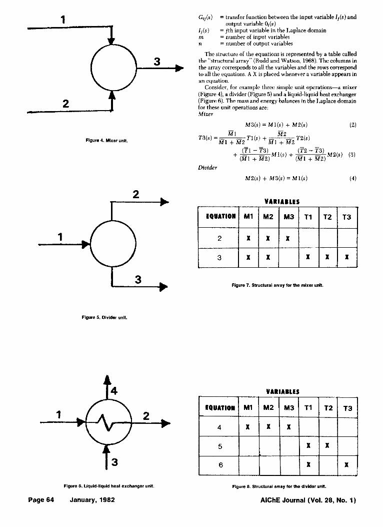
Figure 4. Mixer unit.

13, Figure 5. Divider unit.

1 2

Figure 6. Liquid-liquid heat exchanger unit.

Page 64 January, 1982

G&)

l i ( s ) m n

= transfer function between the input variable I j ( s ) and

= j th input variable in the Laplace domain = number of input variables = number of output variables

output variable Oi(s)

The structure of the equations is represented by a table called the “structural array” (Rudd and Watson, 1968). The columns in the array corresponds to all the variables and the rows correspond to all the equations. A X is placed whenever a variable appears in an equation.

Consider, for example three simple unit operations-a mixer (Figure 4), a divider (Figure 5) and a liquid-liquid heat exchanger (Figure 6). The mass and energy balances in the Laplace domain for these unit operations are: Mixer

M 3 ( s ) = Ml(s) + M 2 ( s ) (2)

W s )

(T2 - T3) (M1 + R2)

R1 G2

(Tl - 73)

7-3(s) =al + w2 T l b ) + -

+ (R1 + G2)

M1 +a2

M a s ) (3) Ml(s ) + - Divider

M 2 ( s ) + M 3 ( s ) = Ml(s ) (4)

EQUATION M1

Flgure 7. Structural array for the mixer unit.

VARIABLES

Figure 8. Structural array for the divider unit.


V I R I A H I S

10 X X X x x

Figure 9. Structural array for the heat exchanger unlt.

T2(s) = Tl(s) (5)

T3(s) = Tl(s) (6) Note that in the above equations the dynamics of the mixer and divider units have been neglected and it has been assumed that the specific heats for all the streams are equal and constant. Heat Exchanger (Mozley, 1956)

M2(s) = Ml(s)

M4(s)=M3(s) [Urn lC l + MlClM3C3](7,S + 1)

T2(s) = 47%' + ~ { T Q S + 1)

(DA)' (T4 - T2) M ~ c Y ( T & s ~ + 2{7@ + 1)

+ I-

where

c3w* M3C3 + VA

7 1 = -

c 1 w MlCl + UA

7; = - -

a = UA[Clal + C3a3] + ClGlC3a3 (13)

79 = dclw-C3w*/(Y (14) C l W C S 3 + C3W*ClGl + UA [ClW + C3Wf]

2 7 ~ " { =

(15) In the heat exchanger equations it has been assumed that the fluids are well-mixed on each side and the specific heat for the two streams are constant.

The structural arrays for the mixer, divider and heat exchanger are shown in Figures 7 ,8 and 9 respectively.

At the causal level, the cause-and-effect relationships of the

n

Figure 10. Cause-anddact graph for the mlxw unit. Figure 10. Cause-anddact graph for the mlxw unit.

Figure 11. Cause-and-effect graph for the divider unit.

n

Figure 12. Cause-and-effect graph for the heat exchanger unlt. Figure 12. Cause-and-effect graph for the heat exchanger unlt.

system are represented by a directed graph G = G ( N , E ) , where N is a set of nodes representing process variable deviations in the laplace domain and E c GXG is a set of directed edges wbch

AlChE Journal (Vol. 28, No. 1) January, 1982 5

I 1 I VARIABLES 1

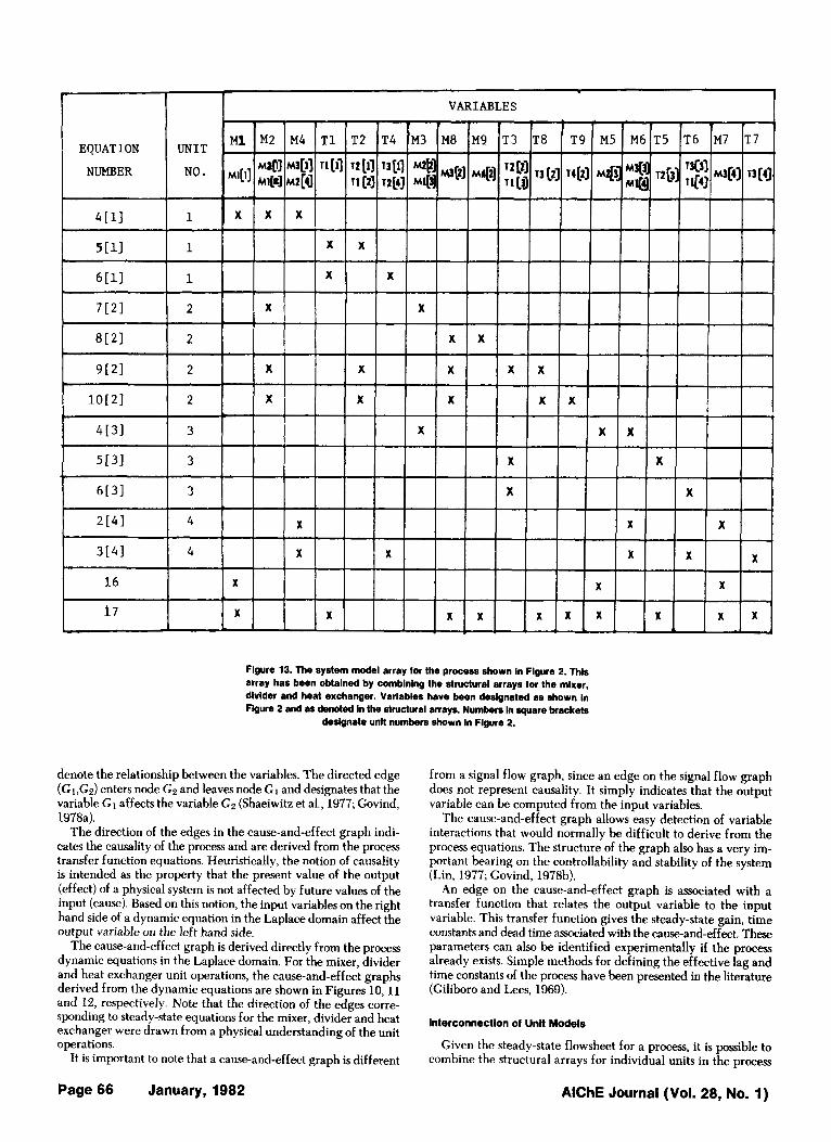
Figure 13. The system model array for the process shown in Figure 2. This array has been obtained by combining the structural arrays for the mixer, divider and heat exchanger. Variables have been designated as shown in Figure 2 and as denoted in the structural arrays. Numbers in square brackets

designate unit numbers shown In Figure 2.

denote the relationship between the variables. The directed edge (G1,C2) enters node Gz and leaves node G1 and designates that the variable GI affects the variable Gz (Shaeiwitz et al., 1977; Govind, 1978a).

The direction of the edges in the cause-and-effect graph indicates the causality of the process and are derived from the process transfer function equations. Heuristically, the notion of causality is intended as the property that the present value of the output (effect) of a physical system is not affected by future values of the input (cause). Based on this notion, the input variables on the right hand side of a dynamic equation in the Laplace domain affect the output variable on the left hand side.

The cause-and-effect graph is derived directly from the process dynamic equations in the Laplace domain. For the mixer, divider and heat exchanger unit operations, the cause-and-effect graphs derived from the dynamic equations are shown in Figures 10.11 and 12, respectively. Note that the direction of the edges corre- sponding to steady-state equations for the mixer, divider and heat exchanger were drawn from a physical understanding of the unit operations.

It is important to note that a cause-and-effect graph is different

from a signal flow graph, since an edge on the signal flow graph does not represent causality. It simply indicates that the output variable can be computed from the input variables.

The cause-and-effect graph allows easy detection of variable interactions that would normally be difficult to derive from the process equations. The structure of the graph also has a very important bearing on the controllability and stability of the system (Lin, 1977; Govind, 1978b).

An edge on the cause-and-effect graph is associated with a transfer function that relates the output variable to the input variable. This transfer function gives the steady-state gain, time constants and dead time associated with the cause-and-effect. These parameters can also be identified experimentally if the process already exists. Simple methods for defining the effective lag and time constants of the process have been presented in the literature (Giliboro and Lees, 1969).

interconnection of Unit Models

Given the steady-state flowsheet for a process, it is possible to combine the structural arrays for individual units in the process


Figure 14. Sydem cause-and-ellect graph tor the process shown In Figure L.

to obtain the system array for the complete process. Additional equations from the steady-state overall mass, energy, and momentum balances that arise due to feedback and feedforward loops in the Process Flowsheet Graph are introduced at this stage and the system array is modified to include these extra equations. For the heat exchange process shown in Figure 2, the structural arrays for the mixer, divider and heat exchanger shown in Figures 7 , 8 and 9 respectively, are combined to obtain the system array for the process, shown in Figure 13. The steady-state overall mass and energy balances arising due to a feedforward loop in the process flowsheet graph (Figure 3), i.e., (Ml, M2, M3, M6, M7; M1, M4, M 7) are:

These overall equations have been shown in the system array. The cause-and-effect graph for the individual units in the process

are also interconnected to obtain the system cause-and-effect graph for the process. This system graph gives all known interactions between the process variables. By tracing paths in this graph, it is possible to find which variables affect a specific process variable or which variables are affected by the given variable. For the process shown in Figure 2, the cause-and-effect graphs for the mixer, divider and'heat exchanger shown in Figure 1 0 , l l and 12 respectively, are interconnected to obtain the system cause-and- effect graph for the process, shown in Figure 14.

AlChE Journal (Vol. 28, NG. 1) January, 1982 Page 67

The system array and the system cause-and-effect graph r e p resent different aspects of the process and will be used in the synthesis of process control systems.

Speciflcatlon of Control Constralnts

Following the generation of the system array and cause-and- effect graph, the control objectives may be specified. These objectives define the variables that need to be maintained within a certain error bound around the steady-state value. In the following section these variables will be termed constraint oariables.

Consider the heat exchange process shown in Figure 2. The process objectives dictate that the temperature of steam 3, T3 be maintained at a specific value. This objective translates into a constraint on the variable T3.

It is important to check the consistency of constraints in order for the control objective to be realizable. It is necessary to know whether they interact since the control structures generated subsequently to satisfy the constraints will also be interacting. A preliminary analysis is done at this stage to arrive at a set of consistent process variable constraints for which control structures will be synthesized subsequently. The problem for checking for consistent constraints is not an easy one. The interactions between mass energy, and momentum balances as well as degree of freedom constraints due to equilibrium etc., must be checked. The details of an algorithm for this task have been presented (Govind, 1978b).

SENSED VARIABLE SELECTION

The problem of sensed variable selection involves: ( 1 ) finding the correct variables to measure; and (2) of measuring or calculating a true representation of the variable. The sensed variable possibilities are expressed by the Sensed Variable Tree consisting of AND-OR gates. A set of variables are ANDed with respect to a constraint variable on the tree if all the variables have to be measured in order to obtain the value of the constraint variable. If a single variable alone is sufficient to obtain the constraint, then the variable is ORed on the Sensed Variable Tree.

The sensed variable possibilities vary in their degree of inference. No variable is ever directly measured. There is always an inference mode.

In addition to the degree of inference, the measurement of the constraint variable is limited by several factors that affect the overall accuracy. These factors are:

(a) Transducer characteristics-nonlinearity, irreproducibility,

(b) Installation characteristics-physical location of the sensor and

The overall accuracy of the measurement is considered with respect to its cost, i.e., cost of the sensor. If the cost to attain a desired accuracy is high, other sensed variable possibilities may have to be considered.

Inferential measurements are only used in instances when a “direct” measurement is not available or prohibitively expensive. The variable most commonly inferred is composition, because of the lack of reliable, rapid and economical analysis for a wide spectrum of chemical systems. Some of the common inferential measurements used in the chemical process industry have been given by Shinskey (1967).

Computing the constraint variable from other variable measurements is generally employed in digital systems, although simple computation may be easily implemented in analog designs. The validity of computed values is affected by simplifying assumptions, such as no heat loss, linearity, 100% efficiency, no change in the equipment parameters over a period of time, as well as the accuracy of the computation.

Sensed variable possibilities which involve computation of the constraint variable are obtained from the system array. The search is for equivalent variables to the constraint. The AND is to indicate that other variables may influence the perception of the constraint

hysteresis, deadband response time, environmental effects

noise

and they must be controlled (or known) to allow a correct inference.

Sensed variable possibilities are generated from the system array by identifying an equation in the array which involves the constraint variable. All variables that are involved in the equation other than the constraint variable are ANDed on the sensed variable tree. Considerations involving measurement and computation inaccu- racy as well as implementation costs are used to evaluate the possibilities. The procedure is repeated for all equations which involve the constraint variable. When all the equations involving the constraint have been used, the constraint variable is replaced by another variable from the tree which is present in the process equations. The procedure outlined above is then repeated for this new variable and terminates when all the variables have been processed.

Sensed variable possibilities are generated by logically simulating the sensed variable tree. For an AND gate on the tree, with N variables, if (N - 1 ) variables are true, the Nth variable is true also. For an OR gate, if any one of the variables is true, the ORed variable is also true. Any set of variables which make the constraint variable true is a candidate sensed variable possibility. The candidate sensed variables are minimized by deleting those candidates for which a subset of variables are sufficient to compute the constraint variable. This ensures that a minimum number of variables are sensed for any given sensed variable candidate.

Consider the process shown in Figure 2. The system array for the process is shown in Figure 13. Process objective dictate a constraint on the temperature of stream 3, T3.

For purposes of illustration assume that T3 can be measured directly with acceptable accuracy. Hence, T3 is placed on the sensed variable tree as shown below:

Constraint T3

T3 I

Since there is no need to infer the constraint T3, the possibility of computing the constraint variable will now be explored. The variable T3 is involved in Eqs. 9[2] , 5[3] and 6[3]. Equation 9[2] is Eq. 9 in this paper written for unit [2] , as shown in Figure 2. Using the procedure discussed before the following sensed variable tree is obtained.

Constraint T3

I T3

OR I

AND T5 T6

M 2 M8 T 2 T8

It is possible to infer the measurements M2 and M 8 from corre- sponding velocity and differential pressure measurements. These possibilities will not be developed in subsequent developments of the sensed variable tree.

The procedure is repeated for M2, T2, T5 and T6, and the following sensed variable tree is obtained.

AlChE Journal (Vol. 28, No. 1) Page 68 January, 1982

Constraint T3

T3

I OR

AND T5 T6

M2 M8 T2 TS AND

I l l OR M9 T1

M3 AND

i? MI M4

T7 M6 M4 T4

I 1 I AND

r-l M6 M7

I AND

I AND

Some of the candidate sensed variable possibilities obtained by logically simulating the tree are:

T3, T5, T6, (M2, M8, T2, T8); (M3, M8, T2, T8), etc.

The sensed variable possibilities can be classified into 3 subsets based on the system cause-and-effects. These subsets are used in the systematic generation of feedback, feedforward and cascade control structures. These three (3) subsets are defined as follows:

The sensed variable possibility is the same as the primary constraint variable or consists of variables which are affected by the constraint variable on the system cause-and-effect graph. For example, constraint on variable T3 (Figure 2) generates the sensed variable candidates T3, T5 and T6. The first variable is the same as the primary constraint variable while the other two are the “down-stream’’ variables. Note that the “down-stream” variables are used only to infer the primary constraint variable.

2. The sensed variable possibility consists of variables all of which affect the primary constraint variable on the system cause-and-effect graph. For example, in the case of the process shown in Figure 2. the candidate (T2 T8, M 2 , M8) would be classified in this subset. These are the “upstream” variables and lead to strategies which control “all” the inputs in order to control the constraint.

3. Sensed variable possibilities that consist of a combination of the above variable subsets or cannot be classified as any of them.

Sensed variable possibilities classified under subset 1 will be. used for the synthesis of pure feedback control structures. Those classified as subset 2 will be used to synthesize pure feedforward control structures. Subset 3 can be used to generate structures that are neither pure feedback nor pure feedforward. A discussion on the synthesis of such structures will be presented in subsequent p u b lications. Cascade structures will be generated by combining feedback and feedforward structures.

1.


Here we use feedforward and feedback in the sense of how the constraint is propagated and not the information flow in the control loop itself. Note that feedback control on “all” the variables “up stream” from the constraint is feedforward by this definition.

SYNTHESIS OF PURE FEEDBACK CONTROL STRUCTURES

Feedback control structures are generated by combining sensed variable possibilities classified in subset 1 with possible manipulated variables, obtained from the system cause-and-effect graph. These variables called subgoals consist of flowrates or pressures (valve positions, motor speeds, etc.), which when manipulated will be able to control the constraint variable. The possibilities of manipulated variables are expressed using a subgoal tree consisting of ANDOR gates.

A set of process flowrates or pressures are ANDed with respect to a constraint variable, if all the flowrates or pressures have to be manipulated in order to control the constraint variable. If a flowrate or pressure is sufficient to control the constraint, an OR gate is used on the subgoal tree. Why the AND’S and OR’S are combined in a particular manner depends on a logic similar to that used for the sensed variable selection, as mentioned above. However, different criteria are used to determine feasibility-steady state gain, dynamics, ease of manipulating variables, range etc., are all important in the evaluation.

The procedure for generating the subgoals is shown in Figure 15. The procedure begins with a constraint variable M. In step [I], the system cause-and-effect graph is examined for a varible (designated X) which affects M but is not already on the subgoal tree. X can be the same as M. Specific heuristics are used in step [2] to judge whether X can be manipulated. Some of these heuristics are:

1. Flows are more difficult to manipulate when: (a) the flow is very large; (b) the flow is a slurry, or solids; (c) the flow has corrosive materials; and (d) the flow is at a very high temperature.

2. Pressures are difficult to manipulate when: (a) the liquid is very volatile (flashing); (b) the fluid is a two-phase mixture; and (c) solids are present.

3. Temperatures and concentrations cannot be manipulated directly in a chemical process.

4. Flowrates or pressures which cause a large number of variables to vary in the process should not be manipulated, if at all possible.

If X can be manipulated and X is the same as M , variable X is ORed with respect to M on the subgoal tree in step [4]. However, if X is not the same as &f, the net gain between X and M is compared with a lower limit G* set by the user. If the gain G is greater than G*, the net dead time between X and M is compared with an upper limit 7; set by the user. In step [7], the net time constant(s) or the dominant time constant between variable X and M is compared with user set limit 7;. If the net gain between variables X and M is lower than the limit G*, specified by the user, the type of cause-and-effect path between X and M is examined in step [a]. If the cause-and-effect path is serial, X is not suitable for controlling M since the gain is not sufficiently large and the procedure returns to step [ 11.

In step [9], if variable X is at the beginning of a negative feedforward loop (Govind, 1978a) variables X and the negative feedforward loop variables are A N N on the subgoal tube, in step [ lo]. The reason for the AND gate is because a change in variable X will not have any effect on the constraint variable M due to a cancel- lation of effects on the two edges of the feedforward loop. However, manipulating both X and the other feedforward loop variables, will affect the constraint variable M .

If X is not on a negative feedforward loop, the procedure ex- amines the possibility of a negative feedback loop existing between X and M. If such a loop is detected and if the loop is sufficient to control M , as indicated in step [ 121, the procedure returns to step [ 11. If the negative feedback loop is not sufficient for controlling M , variable X is ORed with respect to M on the subgoal tree.

January, 1982 Page 69

Figure 15. Procedure for generating a subgoal tree. M is the constralnl variable. G' Is the minimum allowable galn, 7.0 the maximum allowable dead tlme and

T:, the maximum allowable tlme constant set by the user.

When no new variables can be found on the cause-and-effect graph in step [ 11, the entire subgoal tree has been developed. If the subgoal tree does not have any variables, the process system will have to be modified to introduce new manipulated variables. Table 1 contains a list of system modifications that might be necessary to get suitable manipulated variables in a chemical process, for a given constraint variable. This point in the algorithm illustrates, in another way, why process design and control system design should be done simultaneously. The goal is not necessarily better dynamic response in the minimum squared error sense. It is simply to get a variable to manipulate.

The values of user specified limits on gains (C*), dead time (T ; )

and time constant (7; ) depend on the kind of disturbances which affect the constraint variable and the type of control system desired for variable M . If a shutdown system is necessary, the limits on 7; and 7; will be much lower as compared to the values used for normal regulatory control.

For example, consider the process shown in Figure 2. The constraint is the temperature of stream 3, T3. Using the system cause-and-effect graph shown in Figure 14, and executing the procedure shown in Figure 15, the following subgoal tree is obtained.


9 1

I y-&- I I

J. Figure 16. Feedback control structure obtained by chooslng subgoal M6.

->

4 1 Figure 17. Feedforward control structure obtained by combining sensed

variable candidate (M2,M6, R,T6) and wbgoai ME.

4

Figure 16. Cascade control structure obtained by combining feedback control structure shown in Figure 16 with the feedorward control structure shown

In Figure 17.

6

A1ChE Journal (Vol. 28, No. 1) January, 1982 Page 71

Constraint T3 The synthesis problem is subdivided into three subtasks:

able 1. Find possible ways of measuring the process constraint vari-

2. Find possible ways of manipulating the constraint variable 3. Combine solutions of subtasks 1 and 2 to generate feedback,

feedforward, and cascade control structures

The synthesis procedure presented in this paper is our initial solution to the three subtasks mentioned above. Future work to further develop and automate the procedure is needed before it can be applied to large industrial problems.

I OR

M8 M2

I OR

M4 M1 M 3

Choosing a subgoal from the subgoal tree generates a feedback control structure. For example, choosing subgoal M8 gives the feedback control structure shown in Figure 16.

SYNTHESIS OF FEEDFORWARD CONTROL STRUCTURES

A feedforward control system is one in which information from variables that effect the constraint variable is used to control the constraint. Whenever a disturbance occurs, corrective action starts immediately to cancel the disturbance before it can affect the constraint variable.

Synthesis of feedforward control structures involves combining possible ways of computing the constraint variable with possible ways of controlling it. Possible ways of computing the constraint variable were generated in thes sensed variable selection section of this paper. Possible ways of controlling the constraint variable are represented by the subgoals generated in the previous section. Each combination of a sensed variable set classified in subset 2 and a subgoal represents a feedforward control structure.

For example, consider the process shown in Figure 2. Some of the sensed variable candidates to compute the constraint variable T3, and which were classified as belonging to subset 2 are (M2, M8, 2'2, T8), (M3, M8, T2, T8). Some of the subgaals generated for the same constraint in the previous section are M8, M2, M3, and M1. Combining the sensed variable candidates with the subgoals generates a feedforward control structure. One such combination obtained from sensed variable candidate (M2, M8, T2, T8) and subgoal M8 is shown in Figure 17.

SYNTHESIS OF CASCADE CONTROL STRUCTURES

Cascade control structures consist of two controllers arranged such that the output of one controller (called the master or primary) is the set point to the other controller (called the slave or secondary).

Synthesis of cascade control structures is achieved by combining feedback and feedforward control structures generated in the previous sections of this paper. This combination is achieved by replacing the manipulated variable of a control structure with the set point from another control scheme. These combinations would be generated if the set point variables of the synthesized feedback control structures are treated as process variables that can also be manipulated to control a constaint variable.

For the process, shown in Figure 2 if the synthesized feedback control structure shown in Figure 16 is combined with the feedforward structure shown in Figure 17 the cascade control structure shown in Figure 18 is obtained.

In summary, this paper addresses an important aspect of control system design-synthesis of the control structure. It assumes that process cause-and-effects are deterministic and that in order for control to exist, there must be a causal path between the controlling and the controlled variables.

NOTATION

m n

S = laplace transform variable A Cl,C3,

Gij(S)

= number of input variables in a unit operation = number of output variables in a unit opera-

tion

= area of heat transfer (m2) = specific heats of liquid streams, 1, 3, 8 and 9

= transfer function, in the laplace domain, between input variable I j ( s ) and output variable O h )

= user set limit on the minimum allowable steady-state gain between two process variables

C8,C9 respectively

G*

I, (s 1 M = constraint variable M 1,M2. . .M9

Ml(s),M2(s),

= jth input variable in the laplace domain

= mass flowrates of the respective process streams

= Laplace transformed deviations in the mass flowrates for streams 1, 2, 3 and 4 respectively

MI,. . .M8,M9 = steady-state flowrates for the respective process streams

01 (8 1 T1,T2. . .T9

Tl(s),T2(s),

(kg/h)

M3(s),M4(s) - -

= ith output variable in the laplace domain = temperatures of the respective process streams

("(3 = Laplace transformed deviations in the tem-

peratures for streams 1, 2, 3 and 4 respec- T3(s),T4(s) - Tl ,T2. . .T9 - U W

W*

X

Greek letters

a 7

71 71)

79 7 2

Ti:

Subscripts

i i

tively

process streams = steady-state temperatures for the respective

= overall heat transfer coefficient = liquid holdup on the tube side of the exchanger

= liquid holdup on the shell side of the exchanger

= variable on the system cause-and-effect

(kg)

(kg)

graph

= variable defined in Eq. 13 = time constant between two process variables = defined in Eq. 11 = dead time between two process variables = time constant defined in Eq. 14 = defined in eq. 12 = user set limit on the maximum allowable time

= user set limit on the maximum allowable

= damping coefficient defined in Eq. 15

constant between two process variables

deadtime between two process variables

= ith output variable = j th input variable


LITERATURE CITED

Bristol, E. H., “On a New measure of Interaction for Multivariable Process Control,” Trans., IEEE (January, 1966).

Buckley, P. S., Techniques of Process Control, John Wiley and Sons, Inc., New York (1964).

Cadman, T. W., “Application of Linearized Feedfonvard Control to Continuous Flow Stirred Tank Reactors,” M. S. Thew Camegie I d t u t e of Technology (1954).

Foss, A. S., “Critique of Chemical Process Control Theory,” AZChE J., 19, No. 2, p. 209 (March, 1973).

Giliboro, L. G. and F. P. Lees, “The Reduction of Complex Transfer Function Models to Simple Models Using the Method of Moments,” Chern. Eng. Sci., 24, p. 85 (1969).

Govind, R., “Causal Modeling of Large Scale Complex Systems,” Pro- ceedings of the Ninth Annual Pittsburgh Conference on Modeling and Simulation, 9, p. 689 (1978a).

Govind, R., “Control System Synthesis Strategies,” Ph.D. Thesis, Carne- gie-Mellon University (1978b).

Kestenbaum, A., R. Shinnar and F. E. Thau, “Design Concepts for Process Control,” ZGEC Process Design and Deoelopment, 15, p. 2 (1976).

Lee, W., and V. W. Weekman, Jr., “Advanced Control Practice in the Chemical Process Industry: A View from Industry,” AZChE J., 22, p. 27 (1976).

Lin, Ching-Tai, “Structural Controllability,” IEEE Transactions on Au- tomatic Control, AC-19, No. 3 (June, 1974).

Morari, Manfred, Y. Arkun and G. Stephanopoulos, “Studies in the Synthesis of Control Structures for Chemical Process,” AIChE 1.. 26, p. 220 (1980).

Mozley, J. M., had. Eng. Chem., 48, p. 1235 (1956). Newell, A,, J. Shaw, and H. Simon, “Report on a Genera Problem-Solving

Proeram.” Proc. Intern. Conj. Inform. Process, UNESCO House, Paris, - .

p. 2& (ibm). Niederlinski, A,, “Twevariable Distillation Control: Decouple or not de-

coude.” AZChE I., 17,1261 (1971). Nib;, N. J., P r o k m Solving Methods in Artificial Zntelligence, McCraw

Hill, New York (1971). Rudd, D. F. and C. C. Watson, Strategy of Process Engineering, John

Wiley 81 Sons, New York (1968). Sargent, R. W. H., “The Decomposition of Systems and Procedures and

Algebraic Equations,” paper presented at Dundee (July, 1977). Shaeiwitz, J. A., Steven A. Lapp and Gary L. Powers, “Fault Tree Analysis

of Sequential Systems,” ZGEC Process Design and Deuelopment, 16, No. 4 (1977).

Shinskey, F. G., Process Control System, McGraw Hill Co. (1967). Weber, R. and C. Brosilow, “The Use of Secondary Measurements to Im-

Manuscrfpt receiwd March 26,1980, reofdon receioed February 25, and accepted March 18,1981.

prove Control,” AZChE J., 18 (May, 1972).

Purification of Phenolic Wastewater by Parametric Pumping: Nonmixed Dead Volume Equilibrium Model

A new process for purification of phenolic wastewaters by parametric pumping is presented.

An equilibrium (linear) model for nonmixed dead volumes thermal direct mode parametric pumping is developed and the influence of bottom and top dead volume magnitudes on transient separation is analyzed.

Analytical solutions for batch, continuous and semicontinuous operations are presented.

Experimental data on the system phenol/water-Duolite ES861 include equilibrium isotherms at 20°C and 60°C and parapump runs for the cases mentioned above.

C. A. V. COSTA and A. E. ROMllGUES

Chemical Engineering Department UnlverrHy ol Port0

Port0 codex, Portugal

and GEORGES GREVILLOT and DANIEL TONDEUR

Laboratolre des Sclences du Wnlo Chlmlque

Nancy, France CNRS-ENS=

SCOPE

Adsorption is often used as secondary or polishing treatment of phenolic wastewaters.

Recently macrorecticular polymeric resins have been used instead of activated carbon as adsorbent. This is due to easier regeneration and better mechanical resistance although their cost is higher.

However, this operation involves various steps: saturation, regeneration, washing, etc. It can be interesting to use parametric pumping as a purification and/or solute recovery tech- nique instead of classic cyclic operation. Advantages of parametric pumping are: continuous operation, use of low potential thermal energy as regenerant (avoiding regenerant/solute

Conespondence concerning this paper should be a d d d to C. A. V. costn. 0001-1541-82504a0073-)2.00 0 The American Institute of Chemienl Engineem. 1882.

separation) and production of clean water and a concentrated phenol solution, simultaneously.

Modelling of parametric pumping processes has interested many authors; equilibrium (linear and nonlinear) and non- equilibrium models, using continuous and staged approaches have been published.

It is important to notice that in a parapump device, what happens outside the column (reservoirs, dead volumes, feed and drawing points) should be taken into account since it defines the boundary conditions of the column. Two main ideas have been used; everything is well mixed or no mixing at all, outside the column. It has been shown that in the latter case a better transient separation can be obtained.

In a real system dead volumes and sometimes part of the reservoirs can be considered as nonmixed. In this paper a non-

AlChE Journal (Vol. 28, No. 1) January, 1982 Page 73

Control system synthesis strategies

Documents

Transcript of Control system synthesis strategies