Desalination, 84 (1991) 3-43 Elsevier Science Publishers B.V., Amsterdam

AN OVERVIEW OF MODERN CONTROL STRATEGIES FOR OPTIMIZING THERMAL DESALINATION PLANTS

Darwish M.K. Al-Gobaisi, Abdul S. Barakzai, A.M. El-Nashar

UATER b ELECTREl!CY DEPAR!I’MENT ABUIXABI-UAE

ABSTRACT

Vater is the essence of life in arid Middle East Countries. The implementation of robust control strategies enhance the efficiency, safety and reliability of the desalination process. A higher degree of automation is essential for today's large scale complex desalination plants. To achieve optimal design and operation of these plants, careful control system design is required. Even when an acceptable design is completed, the question remains as to whether a better design could be found. Conventional techniques provide for analysis and design of the systems which more or less satisfy arbitrary set of performance requirements. However modern control techniques provide an optimum solution based on specified performance index. In this paper an exposition of merits and demerits of conventional and modern control strategies is outlined. A number of optimal procedures that are used for system identification are highlighted. A brief description of Multi-Stage Flash (MSF) desalination process and controls is given. Novel control strategies for a number of important loops of a large MSF desalination plant are presented.

1. MODERN TRENDS IN CONTROLLER DESIGN

The emphasis today is to achieve greater accuracy and efficiency in control system design by assigning performance index. In

3

4

conventional control, the specifications are in terms of percent overshoot, bandwidth, settling time etc., whereas in modem control, it is given by optimal criteria such as minimum energy , minimum cost and minimum time operation.

Modem 32-bit microprocessor based controllers have the capability, speed and computing power to handle control applications varying from simple PID functions to complex plant optimization. This has opened the way for the implementation of the advanced control strategies based on modem control theory that was formerly possible only with a process computer[18,39,40,42,51]. Most classical control techniques were developed for linear constant coefficients systems with single input single output

(SISO), however when the system contained nonlinearities, dead time and auxiliary parameter variations these techniques could not coupe efficiently . The state variable and polynomial approaches of the modern control theory provide uniform and powerful methods for representing the system of arbitrary order, multiple input multiple output (MIMO), linear or non-linear, time varying or with constant co-eff icients. The state variable approach is used in pole assignment where the closed loop eignvalues are placed in the desired locations. In optimal control the required performance index, being function of states and inputs is to be minimized. The polynomial system approach is useful in the area of adaptive control while the modem control theory forms a basis for process optimization. However we should look at classical techniques as augmenting modem control concepts.

Advanced control includes: System Modelling, Process Identifica- tion, State and Parameter Estimation, Optimal Control, Predictive Control, Adaptive Control, Controller Tuning by Expert System, Heirarchical Control, Process Operation Optimization. The last 25 years have been an era ‘of rapid progress in control engineering such as the development of control methods based on state space, which forms the backbone of the modem control theory. This has been successfully implemented in aerospace industry, power generation, electric power systems, chemical processes and many other fields . These approaches require reasonably good mathematical models of the system to be controlled. Sophisticated identification methods were developed in the early and late seventies that allowed the designer to empirically obtain a good mathematical model of the process. However the adaptive control

5

approach eliminates the need for accurate models and is suitable for the control of time varying processes.

The potential industry user of advanced control techniques has been discouraged by the complex and time consuming computations. Fortunately this problem is now disappearing with the advent of computer aided design (CAD) packages for control systems (i.e. SIMMON, IDPAC, ACET, MATRIX, CTRL, ADAPTECH, CC, etc.).

The system representation in state space form based on a given performance index is utilized for possible optimization. The classical treatment of control system design and analysis is based

on the frequency domain techniques utilizing the laplace or Z- transforms. In most practical implementations based on classical control theory, the concept of single output feedback is used. On

the other hand the modern control theory has the ability to feedback all the state variables. In principle this later concept eliminates the need for dynamic compensation in the controller itself, a topic which constitutes a major portion of the classical control theory. In the case of unavailability of the state variables, the observer forming an integral part of the modern control theory is used.

The automatic tuning for a PID regulator improves the control performance and is superior to the manual, time consuming tuning procedure. The plant dynamics are estimated via least squares scheme and the regulator is tuned by minimizing of the quadratic performance index.

The application of all these methods in the desalination field is likely to result in a better understanding of the process dynamics and thus enhance the control of the process. In this paper we will attempt to highlight the salient features of various types of modern control strategies and background material related to the design of controllers based on classical and modem control theory. Furthermore it is intended to be tutorial in nature.

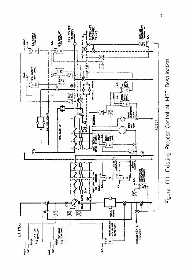
2. PROCESS DESCRIPTION AND CONTROLS

The desalination (Figure 1) is basically an evaporating and condensing process. The heat required for evaporation can be

6

recovered during the condensing phase with a subsequent drop in temperature. MSF distillation is a type of evaporation with many technical and economic advantages and can be regarded presently as providing the optimum solution to the problem of sea water desalting.

The MSF basic layout consists of a steam source, a water/steam circuit (brine heater) and an evaporator unit. The plant includes brine heater, heat recovery and heat rejection stages. The number of stages are determined according to the plant capacity and the performance ratio required. Optimum performance ratios are established on a case by case basis depending on fuel costs, quantity of distillate required, purpose and the usage of plant.

The evaporator can be considered as consisting of three parts; heat rejection, heat recovery and brine heating.

Each MSF evaporator stage includes: - a weir box to control brine level, - a demister to intercept brine droplets, entrained vapours and

prevent them from being carried over the condenser, - a distillate trough under the condenser leads distillate from

one chamber to the next, - an extraction pipe leading to ejectors removes uncondensable

gases from the chamber to create vacuum.

Chlorinated sea water from the sea water supply system enters the plant and flows through the condenser tubes of heat reject stages, gaining heat through condensation of the vapours from the flashing brine on the outside of the condenser tubes. Most of the cooling water heated in this way returns to the sea as heat reject flow. A part of the sea water from the heat reject section is returned to the brine side of the dearator as make-up feed which is chemically treated.

The required make-up is added to the recirculating brine that flows through the condensers of heat recovery stages. Here it absorbs the latent heat of the vapour thereby raising its

temperature and finally flows out from the condenser in the first stage . It then enters the brine heater and is heated by steam to its top temperature. In the case of dual purpose plants the low

pressure steam of extraction or exhaust from the turbine is also used as heating source.

The brine flows from one stage to the next via a flashing device which has a mechanically adjustable orifice to achieve regulation of the brine level in each stage. The stages are water sealed from each other to prevent pressure equalization between stages.

Heated brine flows from the brine heater into the bottom of first stage of the heat recovery section. Since it is warmer than the condenser tubes it flashes and vaporizes, and the vapors are condensed by each stage condenser producing distillate.

The brine at its lower temperature flows through the interstage transfer orifices into the next stage whose internal temperature is a few degrees lower than the previous stage, evaporation and condensation are repeated and finally enters into the flash chamber of the last stage and here make-up sea water is added to it.

Due to vapour flashing the salt content of brine gradually increases stage by stage. To prevent the salt content increase in brine, the concentrated brine is extracted from the last heat reject stage and discharged to a culvert and an equal amount of rejected brine is taken as feed. It is to be noted that this make-up feed water is in addition to the feed water required to replace the distillate.

The distillate is called fresh water or desalted water. The distillate from each stage is collected via distillate trays to the distillate box in the last stage and sent to the water storage tanks.

PERTINENT CONTROL SYSTEMS

About twenty closed loop controls are found in a large scale MSF desalination plant. The following four main loops influence the production rates of the distillate:

1. Top Brine Temperature:

Brine temperature at the brine heater outlet is controlled by actuating the main LP steam control valve to the heater.

2. Brine Recirculation Flow:

Flow rate signal from electromagnetic flov transmitter is used to actuate the respective control valve. The objective is to maintain the brine recirculation with respect to the distillate production rate.

3. Sea Water Flow to the Heat Reject Section:

Sea Water flow to the heat reject section depends on seasonal conditions (summer or winter) and is maintained by actuating the sea water reject control valve or by changing the speed of the sea water supply pump.

4< Last Stage Brine Level:

Brine level in the last stage chamber of the evaporator, which is directly related to the levels in preceding stages, is maintained at a predetermined setpoint. The level controller actuates the brine blow down control valve or changes the speed of the brine blow down pump.

The following additional closed loops are integrated in the

overall control scheme to enhance performance: 5. Chemical inject ion loop, 6. Sea water make up flow loop.

Further improvements are obtained when the following closed loops are added:

7. Distillate level in the last stage, 8. Brine blow down flow, 9. Sea water recirculation, 10. Heat reject section inlet temperature.

The controllers normally employed have PID function on temperature and analysis variables and only PI on the rest of the variables.

LP.S

TtXM

e_

,

CQ

IC. -

CO

ND

ENSA

TE

HEA

DER

REJ

ECT

Figu

re

( 1)

E

xist

ing

Pro

cess

C

ontr

ol

of

MS

F

Des

alin

atio

n

_ _

___----

GRWP CONTROL

LEVEL

___ ----

sue GROUP mNr!ax

LEVEL

DRWE CwRa

LEVEL

________

;,“v”,: vu coma

___-----

FINAL CCNTROL

ELEMENTS

___ ---

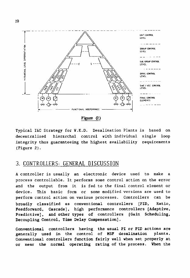
I&C Strategy for W.E.D. Desalination Plants is based on

decentralized hierarchal control with individual single loop

integrity thus guaranteeing the highest availability requirements

(Figure 2).

3. CONTROLLERS: GENERAL DISCUSSION

A controller is usually an electronic device used to make a

process controllable. It performs some control action on the error

and the output from it is fed to the final control element or

device. This basic form or some modified versions are used to

perform control action on various processes. Controllers can be

broadly classified as conventional controllers [PID, Ratio,

Feedforward, Cascade], high performance controllers [Adaptive,

Predictive], and other types of controllers [Gain Scheduling,

Decoupling Control, Time Delay Compensation].

Conventional controllers having the usual PI or PID actions are generally used in the control of MSF desalination plants.

Conventional controllers function fairly well when set properly at

or near the normal operating rating of the process. When the

11

process dynamics or output change then the controller tuning would not be optimal. In other words the fixed optimum tuning would not cover the whole operating range of the controlled process.

In control terms Desalination process may be considered to be sluggish with large time constants, thus manual tuning of PID controller by the plant engineer can be time consuming and inaccurate. Moreover contrary to the normal understanding that MSF desalination plant is simple to operate, thus requiring simple conventional controllers is unrealistic. It is a thermal system, that involves complex dynamics and dead-times. This necessitates use of more powerful techniques than a simple PI or PID controls.

In a large MSF desalination plant with considerable amounts of mass and energy a new type of high performance controllers is highly desirable. These are almost always digitally based and perform control functions based on many available modern control algorithms. This has enabled the control engineers for the first time to successfully implement modern control theory.

The ground work already exists for trying to implement optimal control theory using high performance controllers. This is motiva- ted by the fact that considerable work has been done in the area of optimization of the MSF desalination process from the point of view of the design. Moreover a number of papers have appeared in the literature in the area of process operation optimization based on physical modelling[8,9,23,27,28]. This opens ways and means for trying to implement modern control strategies for process operation optimization. The authors however are not aware of any practical implementation of optimal control strategies or utilization of high performance controllers, resulting in optimum control of desalination plants[1,14,15,17-19,21,22,26,46]. The design technique and theory must be augmented with practical considerations relevant to the MSF desalination plant. From the literature available concerning other applications[39,40,42] it is apparent that the response characteristics of these controllers are far superior thereby giving tighter control resulting in optimization of the overall process.

High performance controllers are generally referred to in literature as those incorporating state of art technology and know how. It is anticipated that application of high performance

12

controllers including setpoint optimization is certain to result in a stable, efficient and smooth operating plant with extended life span.

3.1 PERFORMANCE INDEXES

A performance index should offer selectivity in the optimal adjustment of the parameters and clearly distinguish them from nonoptimal ones. In addition, a performance index must yield a single positive number or zero, the later being obtained if and only if the measure of the deviation is identically zero. A performance index must be a function of the parameters of the system if it is to be useful and it must exhibit a maximum or minimum, resulting in parameter optimized controller. To be practical, a performance index must be easily computed, analytically or experimentally.

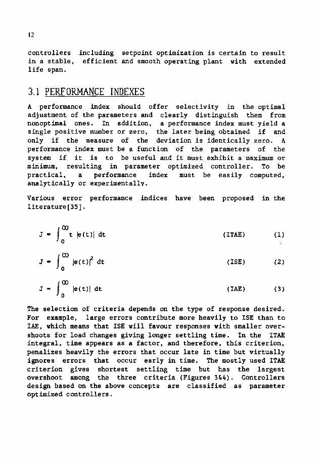
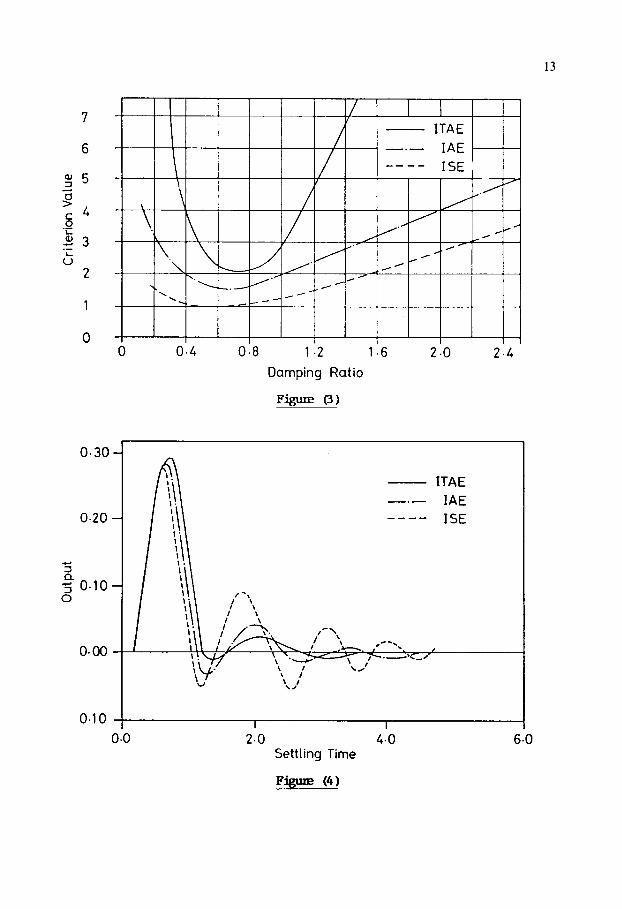
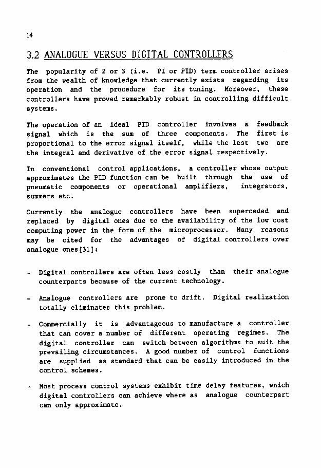
Various error performance indices have been proposed in the literature[35].

03 J- t k(t)1 dt (ITAE) (I)

0

I co

J= /e(t)? dt 0

(I=) (2)

co J- le(t)l dt (IAE) (3)

0

The selection of criteria depends on the type of response desired. For example, large errors contribute more heavily to ISE than to IAE, which means that ISE will favour responses with smaller over- shoots for load changes giving longer settling time. In the ITAE integral, time appears as a factor, and therefore, this criterion, penalizes heavily the errors that occur late in time but virtually ignores errors that occur early in time. The mostly used ITAE criterion gives shortest settling time but has the largest overshoot among the three criteria (Figures 3b4). Controllers design based on the above concepts are classified as parameter optimized controllers.

13

7

6

/ I I

I /

\ I I I/ I I ---- \

ITAEI j-+-t+&/ -.- IAE t---j--~

A._.,/ ‘. _/-

0 0.4 0.8 1 .2 1.6 2.0 2.4

Damping Ratio

FigulE (3)

- ITAE

-.- IAE

---- ISE

2.0 4.0 Settling Time

Figure (4)

6.0

14

3.2 ANALOGUE VERSUS DIGITAL CONTROLLERS

The popularity of 2 or 3 (i.e. PI or PID) term controller arises from the wealth of knowledge that currently exists regarding its operation and the procedure for its tuning. Moreover, these

controllers have proved remarkably robust in controlling difficult systems.

The operation of an ideal PID controller involves a feedback

signal which is the sum of three components. The first is proportional to the error signal itself, while the last two are the integral and derivative of the error signal respectively.

In conventional control applications, a controller whose output approximates the PID function can be built through the use of pneumatic components or operational amplifiers, integrators, summers etc.

Currently the analogue controllers have been superceded and replaced by digital ones due to the availability of the low cost computing power in the form of the microprocessor. Many reasons

may be cited for the advantages of digital controllers over

analogue ones[31]:

Digital controllers are often less costly than their analogue counterparts because of the current technology.

Analogue controllers are prone to drift. Digital realization

totally eliminates this problem.

Commercially it is advantageous to manufacture a controller

that can cover a number of different operating regimes. The

digital controller can switch between algorithms to suit the prevailing circumstances. A good number of control functions are supplied as standard that can be easily introduced in the control schemes.

Most process control systems exhibit time delay features, which digital controllers can achieve where as analogue counterpart can only approximate.

15

- It is much simpler to interface digital controllers to

supervising, monitoring and expert systems than analogue ones.

3.3 DIGITAL CONTROLLERS

The methodology based on conventional design techniques of the

root locus, bode plot or the process reaction curve methods of Ziegler-Nichols may be applied for designing digital controllers.

The procedure would be to first design the analogue form of the controller or compensator to meet a particular performance

specification. Having done this the analogue form can be

transformed to discrete representation by means of the Z-transform

or using difference equations. The most popular and widely used

control algorithm is the three term digital controller and today

virtually all microprocessor based systems commercially available

use this form of controller.

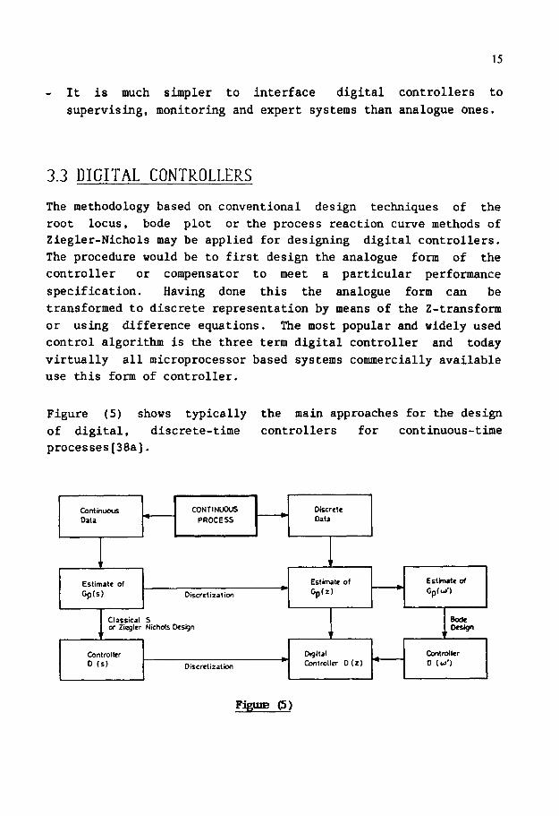
Figure (5) shows typically the main approaches for the design

of digital, discrete-time controllers for continuous-time

processes[38a].

Continuou

O&l

CONTINUDUS Discrete -

PROCESS Data

i

Estimate of

GpW Discrctization

+

Estimate of Estmatc of __c w

Gp(z) Gp(4

OT Ziegler Nichols kSign

1

controller Digital cmtrotlcr

D (5) Discrelizatim * Controller D (2) - 0 (0’)

16

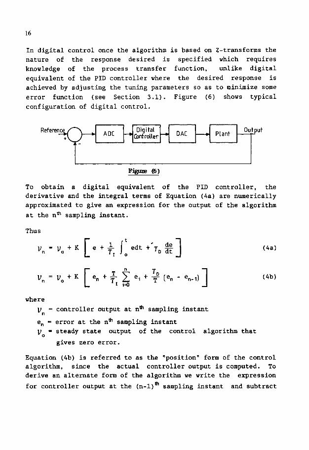
In digital control once the algorithm is based on Z-transforms the

nature of the response desired is specified which requires

knowledge of the process transfer function, unlike digital equivalent of the PID controller where the desired response is achieved by adjusting the tuning parameters so as to minimize some

error function (see Section 3.1). Figure (6) shows typical

configuration of digital control.

, ,

ADC -e Digital

Gmtroller h DAC _+ Plant output

To obtain a digital equivalent of the PID controller, the derivative and the integral terms of Equation (4a) are numerically approximated to give an expression for the output of the algorithm

at the nti sampling instant.

Thus

C n

vn =v/K 7, T (en - en-11 1

where

v" =

en p

VCJ =

controller output at n* sampling instant

error at the nth sampling instant steady state output of the control algorithm that

gives zero error.

(4a)

(4b)

Equation (4b) is referred to as the "position" form of the control algorithm, since the actual controller output is computed. To derive an alternate form of the algorithm we write the expression

for controller output at the (n-l)* sampling instant and subtract

17

Equation (4b) to obtain:

C 7

U” = u,_, + K (e, - e,_,) + F e, + -$ (e, - Zen_, + e,_2 )I

(5) I

Equation (5) is referred to as the velocity form of the PID

algorithm, because it computes the incremental output instead of the actual output of the controller. The velocity form of the algorithm also provides protection against reset windup, because it does not incorporate sums of error sequences and achieves bumpless transfer. However the technical requirements of the sampling theorem must be satisfied [i.e. sampling time is about one-eigth to one-tenth of the dominant time constant]. Further enhancements introduced in recent years have been in the autotuuning of the three-term algorithm using on-line plant identification and computation of an optimum setting for the 2 or 3 term controller parameters.

3.4 DEAD-TIME CONTROLLERS

Thermal processes exhibit[31,44] apparent dead-time characteris- tics and since dead-time is detrimental to control, there is considerable incentive to develop control algorithms that can

compensate for such delays. During dead-time there is no output

in response to the input to initiate corrective action. The sudden increase of steam flow into the brine heater impinges on the

tubes, this may cause errosion and subsequent damage. Moreover,

transient shell over pressure may result in leakage damage of the expansion joint. There are several digital design algorithms such as the following: - Smith Predictor Algorithm, - Dahlin Algorithm, - Analytical Predictor, - Kalman Algorithm.

These controllers are representative of a general class called model based or model predictive controllers since they include

models of dead-time in the process being controlled. Successful

18

application of these controllers require accurate model of the process.

4. SETPOINT OPTIMIZATION

In desalination process, the need for optimization arises both before and after the commissioning of a new plant. The search for the control which attains the desired objective while maximizing or minimizing a defined system criterion constitutes the fundamen- tal problem of optimization theory. Furthermore optimization theory is generally decomposed into static and dynamic problems.

A mathematical model of the desalination plant forms the heart of the control system and is essential in order to carry out the necessary process operation optimization. Indeed the application and augmentation of existing physical modelling schemes with system theoretic techniques will lead to the desired operating objectives.

Generally there are two schools of thought in the choice of mathematical model for use in a control system. One school believes that the model should be based on physical laws that characterise the process. The other school believes that the model should be based on observed relation between input and output of the process or the black box approach. The black box approach is generally preferred by control engineers since the model based on physical laws tends to be extremely complex. Setpoint control based on process optimizing in the desalination context can be defined as an activity for the purpose of achieving and preserving an optimal plant performance. The need for such a design arises due to plant disturbances which have a major impact on the optimal operating conditions. Another level of desalination process control is the so called stabilizing control which may be defined as an activity aimed at minimizing the deviations between the measured variables and their setpoints, naturally considering the later being fixed. The black box approach is based on identification of the process dynamic mode 1 including the static part. For detailed elucidation of the above strategy the following references[13,36,48,54] are suggested.

19

Consider the following performance index or objective function which represents an efficiency or throughput of a non-linear plant model.

J = f(u, y) (6) Y = g(u, t) (7)

where U inputs y outputs

From Equation (6) we obtain static part using final value theorem.

J* - f(Q y*) (8)

Moreover constraints can easily be incorporated in the objective function. The static model is used in the optimizing control to calculate the new values for the manipulated inputs "u". The steady state optimal solution is obtained by using any of the following techniques[l6].

- Penalty function methods, - Iterative linearization methods, - Iterative quadratic programming methods, - Lagrange multiplier methods.

These techniques seek successful better feasible values for the process variables and are applied iteratively until no further improvement in reducing the objective function is found or until some predetermined accuracy has been achieved. Iterative techniques are characterized by the method of selecting a search direction and the distance of movement. In the gradient technique for optimization the cost criterion is used to determine the search direction. Gradient techniques such as GRG and gradient projection methods are considered extremely powerful for solving complex non-linear systems and some of the best non-linear programming codes are available as listed in Table (1).

The above briefly outlined control scheme can also be classified as adaptive because the calculations and implementations of the optimal setpoints are based on a model which is periodically

20

identified on line from the inputs and outputs of the process signals.

Different parameter estimation techniques such as instrumental variables, least squares, extended least squares, maximum likelihood[38,45,50,53] etc. are used to update the process model. A predictive model obtained from on line identification predicts the effects of changes in the independent variables and the objective function at steady state conditions.

Setpoint control in the field of Desalination Process as reported in the literature[l7,19] is mostly based on trial and error methods that do not provide systematic framework from which one could derive a generalized theoretical approach for on-line optimizing control.

The need to operate desalination process optimally is as old as desalination itself but the ability to do this automatically is fairly novel. Techniques for automatic optimization have been available for at least 25 years. Today's powerful microcomputers as required for optimal operation of desalination processes or systems is readily available and cost effective.

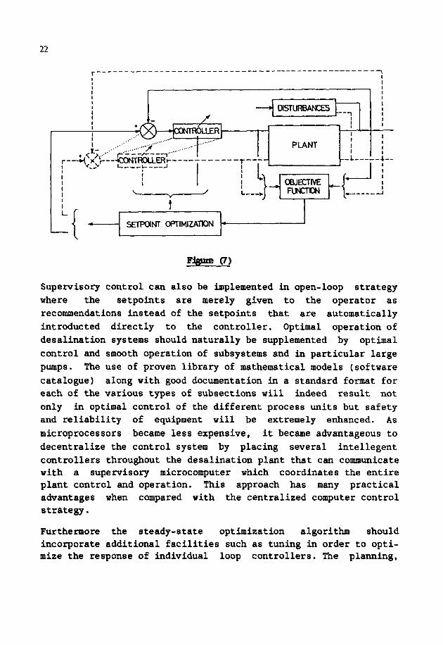
In general there are two types of optimization; steady state and dynamic optimization[29,34,43,49]. Steady state optimization is concerned with the process in the steady state whereas dynamic optimization considers and makes use of dynamic process affects. The steady state optimization is much simpler than that of dynamic optimization and in general is an integral part of the supervisory control. Here slow adjustment of the setpoint of each individual controller for the desalination process (Figure 7) is implemented. Considering the hierarchial control structure, it is at a level above the fast process stabilizing control function. Here supervisory control refers to a methodical, quantitative determination of the optimal setpoint for the process controllers

while satisfying mass and energy balance. In order to implement a supervisory control strategy the algorithm will consist of the following: - A performance index,

- A mathematical model, - A methodology (systematic determination of setpoints).

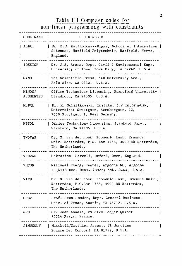
21

Table (I] Computer codes for non-linear programming with constraints

____________________~~~~~~~~~~~~~~~~~~~~~~~~~~~~_~~_~~~~~~~~_~~_~~ 1 CODE NAME 1 SOURCE __ _________ ___-__r_____________~-~~~~~~~~~~~~_~~~~~_~~_~~~~~_~

1 ALRQP I 1 Dr. M.C. Bartholomew-Biggs, School of Information j

I s ciences, Hatfield Polytechnic, Hatfield, Herts, 1 I England.

I ____________ f _D________________-___________-___-_-______-__-____ 1

1 IDESIGN r. J.S. Arora. Dept. Civil & Enviromental Engr, I 1 University of Iowa, Iowa City, IA 52242, U.S.A.

; ____________, ___________________________________________________ /

1 GINO I The Scientific Press, 540 University Ave.,

( Palo Alto, CA 94301, U.S.A. ____________I___________________________________________________~

1 MINOS/ I Office Technology Licensing, Standford University.1

I AUGMENTED 1 Standford, CA 94305, U.S.A. ____________ _______________________~__~__~__~~_~~_~~~~~~_~~_~~_

1 NLPQL I D r. K. Schittkowski, Institut fur Informatik, I I I Universitat Stuttgart, Azenbergstr. 12,

I 7000 Stuttgart 1, West Germany. 1____________ I_______________________________________ _____ _______ I

I NPSOL I Office Technology Licensing, Stanford Univ., I I Stanford, CA 94305, U.S.A.

)____________/___________________________________________________I

I TWOFAS r. G. van der Hoek, Economic Inst. Erasmus I niv. Rotterdam, P.O. Box 1738, 3000 DR Rotterdam,I

I The Netherlands.

( VF02AD I_._____-_____

1 VMCON I

; ____________ j

1 WIEM

I __ _ _ _. __ _ __ __ I

Librarian, Harwell, Oxford, Oxon, England. _-_________-____-___~__~~_~__~~-~~-~~--~-_~~_~~~~~_ I National Energy Center, Argonne NL, Argonne I IL(NTIS Dot. DE83-048922) ANL-80-64, U.S.A. I

-__-_______-__-__-_________________c____~~~~~~~~~~~ Dr. G. van der hoek, Economic Inst, Erasmus Univ., 1 Rotterdam, P.O.Box 1738, 3000 DR Rotterdam,

The Netherlands. I _______________________~__~~_~~~~~~_~__~~_~~~~~~~~~

1. 1 GRG2 I Prof. Leon Lasdon, Dept. General Business, I

I____________ of Texas, Austin, TX 78712, U.S.A.

1 GRG I Dr. Jean Abadie. 29 Blvd. Edgar Quinet

/

I 75014 Paris, France. ~____________1_______________~~__~~_~__~~_~~_~~_~~_~~~~

I SIMUSOLV I Mitchell/Gauthier Assoc., 73 Junction

I 1 Square Dr. Concord, MA 01742, U.S.A.

22

-i I

I I

PLANT I I I

_-I___-_&_ I ’

SETFQINT OPTlMlZATlON 4 I

Supervisory control can also be implemented in open-loop strategy where the setpoints are merely given to the operator as recommendations instead of the setpoints that are automatically

introducted directly to the controller. Optimal operation of desalination systems should naturally be supplemented by optimal

control and smooth operation of subsystems and in particular large

Pumps l The use of proven library of mathematical models (software

catalogue) along with good documentation in a standard format for each of the various types of subsections will indeed result not

only in optimal control of the different process units but safety and reliability of equipment will be extremely enhanced. As

microprocessors became less expensive, it became advantageous to

decentralize the control system by placing several intellegent controllers throughout the desalination plant that can communicate with a supervisory microcomputer which coordinates the entire plant control and operation. This approach has many practical advantages when compared with the centralized computer control strategy.

Furthermore the steady-state optimization algorithm should incorporate additional facilities such as tuning in order to opti- mize the response of individual loop controllers. The planning,

23

design and construction of a large MSF desalination plant is a complex task and involves many professional disciplines.

This also applies to automation of the process and because control is closely related to the process, it is important that the desalination process designer and the control engineer maintain good communication and cooperation. When this is not the case, the result can easily be that the control engineer underestimates or misunderstands the process complex problems and prescribes a control system structure that cannot perform satisfactorily.

Practicing process and control engineers are frequently unaware of the many possibilities available to them, that could bridge a gap between the available control’techniques and the usual practice. The use of simple and generalized control system solution is recommended in most cases.

5. MODERN DESIGN TECHNIQUES

The desalination plant control system has basically to perform three major functions. It must ensure the stability of the process, suppress the effects of external disturbances and achieve a best performance of the process. The subject of control principles, modelling and control system design is very broad. Here modern approaches to control system will be outlined so that a feel for the alternatives and the development in the design methods can be noticed. For the approaches of these methods in detail, it is necessary to study the literature[11,20,24,24a,41]. The approaches are based upon the well-understood and tested techniques developed before and after 1960 by Kalman, Astrom, Athans, Kwe rke rnaak , Grimble, Kailth, Balakrishnan, L iung , Roozenbrok, MacFarlane and many others. Topics such as safety, choice of instrumentation, reliability etc. will be excluded although all these factors must be in the background for a worth while design technique. Having found the optimal values of all the process variables by some optimization technique, we are required to keep the variables at these setpoints. If we exclude external disturbances affecting the process, the problem is formulated as a deterministic dynamic optimization. If we include external disturbances the problem is

24

formulated as stochastic dynamic optimization. Furthermore a mathematical model is prerequisite for optimal controller design. The controller requires information concerning the process dynamics from the mathematical model as well as measurement in order to function properly. This is the subject of state and parameter estimation or identification as it is known from system- theoretic approach.

5.1 STATE FEEDBACK

The classical methods of design feedback use one variable, the output. The conventional controller (PI, PID) is unable to control all system poles. The application of state space concepts in control engineering gave rise to modem control theory[6,25,33] which provides a detailed view of the internal structure of a system. Thus state feedback can be used to change the natural modes of a system; basically to reduce time constants or provide adequate damping of oscillatory modes. In terms of state space concept this amounts to changing the eigenvalues of the system and is referred to as "pole placement". The best design of state feedback requires all the states of the system to be available for feedback. Generally this is impractical and expensive. The state estimation is accomplished by designing a dynamic observer to obtain an estimate of the state vector from the available output vector. Alternatively output feedback can be designed, that is, feedback from output instead of the state.

Consider the discrete state model represented by Deterministic Model[ll]:

X(kt1) = Q(k) X(k) + r(k) p(k) (9) Y(k) = C(k) X(k) (10)

where X -_) N-vector of state, I_L + S-vector of inputs, Y + M-vector

outputs, 0, r, C are [(NxN), (NxS), (MxN)] matrices.

Controllability:

A system is said to be controllable if, for any initial state

X(o), it is possible to find an input which will transfer it to any final state X(N) with finite N. In the pole placement design, it is necessary to inverse the matrix which shall be of rank n.

25

Observability:

A system is said to be observable, provided that the initial state

X(o), for any (X0), can be calculated from the N measurements

Y+,), Ycl) --- Y@_,) with finite N.

In observer design, it is necessary to inverse an observability

matrix.

Stability:

A stable system response requires that the motion converges

asymptotically towards a defined position in state space when

initially displaced. There are many Stability Criteria available

for control systems such as Jury Stability Criteria, Routh Hurwitz

Stability Criterion, etc., however, they are limited to linear

time-invariant systems. An elegant procedure is due to Liapunov

in which single scaler variable is defined as a quadratic measure

of displacement in state space.

Pole Placement [Assignment]

The selection of a feedback gain matrix to position the closed

loop poles is called pole-placement design. The control law is

defined as:

u = -K X(k) (11)

The closed loop system equation is

X(kt1) = [Q(k) - TWK] X(k) (12)

The desired pole locations is determined by

AC = 121 - @ + rK/ = (Z-X,) [Z-X,) --- (Z-X,) (13)

A model must be controllable and observable if feedback is to be

effective in changing it.

Since it is impractical to assume that all the states are

available, an observer is used to estimate from inputs and output

26

the states, however the system must be observable. Furthermore it is assumed that a reliable methametical model is available to generate an estimate of the states.

The pole-placement procedure is applicable for a regulator control system (zero input), and may also be modified to take care of servo control systems (reference input). Moreover the pole- placement procedure presented is basically non-optimal. However, optimal model control is based on this conventional pole-placement but instead of choosing the feedback gain directly, the design parameters of the quadratic cost index i.e. [Q&R matrices] is chosen to achieve this objective (see Equation (14)).

5.2 OPTIMAL CONTROL

The state space methods are perhaps best .known for their association with optimal control. Frequency domain techniques cannot deal precisely with control problems involving one or more of the following constraints[31]. - Limits on the time available to perform a task - Control constraints on magnitydes - Optimum performance involving MIMO - Complex non linearities.

The essential aspects of control problem formulation are: - A specified objective function - A mathematical model to be controlled - Control strategy for measuring performance of any given system - A set of admissible controllers.

Naturally for the purpose of optimal control it is necessary to have a mathematical model for the dynamical system. Generally a mathematical model is represented by a set of first order difference equations.

The most interesting aspect of optimal control is its method of performance assessment. A search for the optimal control or the controller producing the highest performance is a well defined

27

problem of designing the controller that produces the smallest value of the performance index J,.

_ N

J, = - ' k=O

c [XT(k) QX(k) + UT(k) h(k) 1 (14)

The objective is to find control sequence to minimize J, based on

Equations (9) & (10).

To solve the linear quadratic (LQ) regulator problem, we apply the calculus of variations (i.e.. Lagrange approach). Other applicable approaches are; Principle of optimality (Bellman), Minimum Principal (Pontryagin's), etc.

Proceeding with the minimization leads to a set of equations in the original states and a new set of variables called the co- states. The complete solution involves solving the famous Riccati equation. Even when the system and weighting matrices are all time invariant, the feedback gain is still a function of time since Riccati equation's P(k) is time varying.

Thus the optimal control is a time varying state feedback when compared to classical frequency-domain methods. Generally the algorithm is extremely demanding from point of computation, however it is fortunate that as we go to the limit N + ~0 the solution can be considerably simplified. The control law requires the storage of only steady state gain elements of K.

Classical design techniques provide no formal procedure for dealing with noise and disturbance inputs unlike the Linear Quadratic Gaussian (LQG), which gives a systematic approach. The LQG theory provides a synthesis tool and has been applied to produce useful practical controllers for applications in industry[12,39,51]. An advantage of the time domain state-space form of solution is that it includes the Ralman filter. The transposition of the linear quadratic gaussian control into a deterministic control and including a Ralman filter is in fact one of the most interesting features of the LQG solution. The digital design techniques for optimal control applications when used

28

intelligently on system models provide the designer as well as the user with a good chance of success[24].

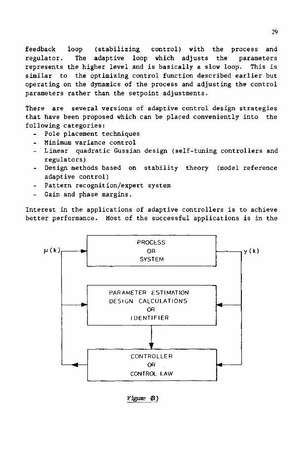
5.3 ADAPTIVE CONTROL

An adaptive control system[7,47] (Figure 8) is one in which the controller parameters are adjusted automatically to compensate for changing process conditions.

The techniques described previously assume that the plant has been perfectly modelled. In adaptive control systems, the system dynamics are assumed to be unknown and the application of classical design criteria are not so appropriate. There are indeed advantages to be obtained by using adaptive control technique with periodic tuning rather than in a full adaptive context, where a major problem is in ensuring that the data used in the estimator is indeed good data.

The controllers (PI, PID) are tuned on-line in order to achieve satisfactory performance of the plant. Some external and internals conditions that require controller retuning because of the process varying conditiong,are a good subject for adaptive control:

- Heat exchanger fouling, - Ambient condition variations, i.e. sea water temperature, - Brine recirculatSon parameters i.e. temperatures, conductivity, - Equipment status changes i.e. start-up, shutdown, sub system

malfunctions, - pH control.

The adaptive control approaches are based upon techniques developed by Astrom and Wittenmark at the Lund Institute of Technology, Sweden. Other researchers who have contributed immensely to the subject of Adaptive Controllers design are Clark and Gawthrop[lO,32], Peterka, Hasting-James, Iserman, Grimble and

many others. The exciting developments derived from the philosophy of optimal control and adaptive control approaches to control system design will be outlined briefly. For detailed elucidation of adaptive control concepts and practical experiences the following references are suggested[3,4].

Astrom (1983) defines adaptive control systems as consisting of two hierarchial levels. The lower level consists of ordinary

29

feedback loop (stabilizing control) with the process and regulator. The adaptive loop which adjusts the parameters represents the higher level and is basically a slow loop. This is similar to the optimizing control function described earlier but operating on the dynamics of the process and adjusting the control parameters rather than the setpoint adjustments.

There are several versions of adaptive control design strategies that have been proposed which can be placed conveniently into the following categories :

- Pole placement techniques - Minimum variance control - Linear quadratic Gussian design (self-tuning controllers and

regulators) - Design methods based on stability theory (model reference

adaptive control) - Pattern recognition/expert system - Gain and phase margins.

Interest in the applications of adaptive controllers is to achieve better performance. Most of the successful applications

PROCESS

p(k)- + OR

SYSTEM

PARAMETER ESTIMATION

+ DESIGN CALCULATIONS

4 OR

I DENTIFIER

v

CONTROLLER

OR 4

CONTROL LAW

is in the

y(k)

30

area of individual loops. Today there are approximately more than

120,000 adaptive loops in operation.

The term adaptive control signifies that the controller performs

to functions i.e. learning about the controlled process and at the

same time controlling its behaviour.

Even though some tuning rules are available (Ziegler-Nichols) the

tuning procedure remains subjective relying heavily on the skill

of the operator. The time consuming and difficult nature of this

procedure results in a poorly tuned control loops giving not the

best achievable performance.

An adaptive controller can be considered as consisting of three

main components:

(1) A parameter estimator that monitors the plants inputs and

outputs and computes the,estimates of the process dynamics

in terms of a set of parameters in a defined structure of a

model of the controlled plant.

(2) A control design algorithm that takes the estimated

parameters and generates controller coefficients.

(3) A controller that accepts the coefficients from the control

design algorithm and computes the required control output.

Previously we have highlighted a number of controller design methods

based on some of the following estimation procedures.

- Recursive least squares,

- Extended least squares,

- Maximum likelihood methods (recursive),

- Instrumental variables.

Different combinations of estimation and design techniques leads

to controller with different properties.

31

There are three basic approaches to adaptive controller design:

(1) Self-tuning control (STC)

(2) Model reference adaptive control (MRAC)

(3) Gain scheduling control.

The method of implementing the system identification determines

the types of adaptive control schemes:

- Implicit adaptive scheme

- Explicit adaptive scheme.

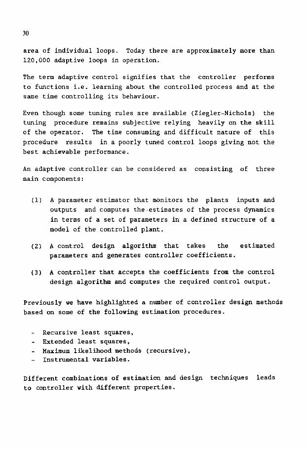
A scheme which separates out the identification and control

calculation is known as an explicit adaptive scheme - (Figure 9).

I I )

Y b COMTROLLER PLANT w

P OUTUJT / A

pigune @)~licitSelf-tXxriQgCultLD1

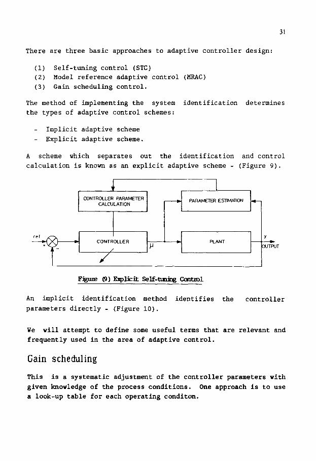
An implicit identification method identifies the controller

parameters directly - (Figure 10).

We will attempt to define some useful terms that are relevant and

frequently used in the area of adaptive control.

Gain scheduling

This is a systematic adjustment of the controller parameters with

given knowledge of the process conditions. One approach is to use

a look-up table for each operating conditon.

32

CONTROLLER PARAMETER

I

ESTIMATION

4

CONTROLLER b PROCESS

/ IJ

/ :-!

Y

PigIl? (lo) Implid self-tuning ConiYDl

This is essentially feedfoxward strategy and represents an open-

loop adaptation of the controller constants because the results of

controller adaptation are not feedback - (Figure 11).

GAIN SCHEDULING 4

I

CONTROLLER

/

/

* PROCESS _ Y

IJ

Auto-tuning

This is related to the auto-tuning of PID parameters and usually

based on pattern recognition.

33

Self-tuning

This is relevant to the application of an advanced control

strategy, based on control law and estimation of the process

parameters. This is an alternative to gain scheduling and

requires good knowledge of process changes that cannot be

anticipated. Self-tuning controller is based on the strategy that

the controller constants are expressed as a function of the

parameters in the process model and are updated on-line as the

process data is received. Alternatively it is also classified as

"self-adaptive" controller. There are three configurations that

can be used to implement self-tuning control strategies as shown

in Figures (9). and (10).

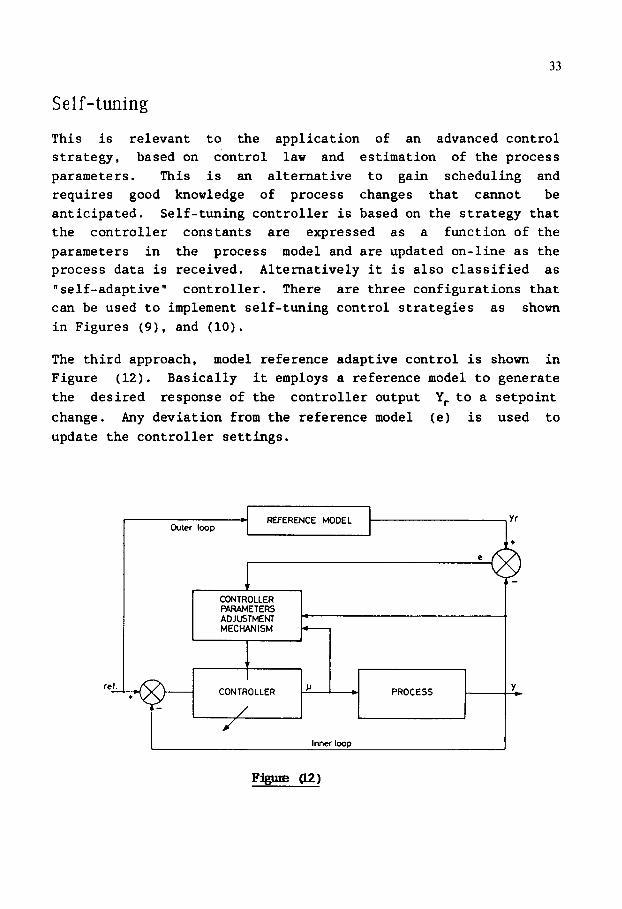
The third approach, model reference adaptive control is shown in

Figure (12). Basically it employs a reference model to generate

the desired response of the controller output Y, to a setpoint

change. Any deviation from the reference model (e) is used to

update the controller settings.

outer loop

CONTROLLER PARAMETERS AOJUSTMEM .

MECXANISt.4 -

CONTROLLER CI L PROCESS Y

/

J

Inner loop

34

Astrom and Wittenmark (1973) developed a single loop adaptive control algorithm for the self-tuning regulator (STR) using minimum variance. Clark and Gawthrop also produced a self-tuning controller, based on the generalized minimum variance control law in terms of a function representing the generalized system output. In all cases the transfer functions are chosen to achieve a desired performance from the system. It should be pointed out that model reference adaptive controllers and self-tuning controllers have been shown to be mathematically equivalent.

Polynomial Equations Optimal control previously has been based on the application of state variables, In this context optimal control of systems described by transfer function is achieved by the application of the Diophantine equation, whereas Riccati equation provides the formal solution in the state space. The approach is mainly based on the polynomial matrix theory of Kucera[37].

Pattern Recognition Pattern recognition is based on a scheme that is able to recognize specific conditions and decide on the necessary corrective action. It is an alternative when compared to adaptive control that requires identification. This controller is based on the so called expert system approach for adjustment of controller parametters. The on-line tuning of the parameters (such as gain, integral and derivative functions, etc.) is based on the closed loop transient response to a step change in set point and by evaluating the salient characteristics of the response (e.g. overshoot, decay ratio and period). The controller parametters can be updated without finding a new process model in quasi-optimal manner.

High Performance Controller It is now a fact that most of these so called high performance controllers are off the shelf items and are available with many manufacturers as mentioned here under: - Satt Control Instruments AB, Solna, Sweden (ECA-04,40,400) - First Control Systems, Sweden - Foxboro, North Haven, USA (EXACT) - Siemens, Erlangen, Germany (SIPART DR 20/22) - Asea Brown Boveri, Sweden (NOVATUNE) - Bailey,Tagata-Gon,Shizuoka-Ken,Japan (ACCORD SYSTEM, EXPERT-go)

35

- Fisher Controls International, Iowa, USA (DPR-900) - Hartmann & Braun, Germany (DIGITRIC P, PROTRONIC P, XU 03/04) - Powell Process Systems, Houston, Texas, USA (MICON S32) - Turnbull Control Systems, Worthing, Sussex, U.K. (63558/63656) - Mitsubishi, Japan (MIDAS 8000) - Etc.

The high performance controllers are structurally more stable and robust because of being less sensitive towards system parameter variations than the simple PID controllers. These incorporate automatic parameter adjustments resulting in tighter process

control. The plant and equipment-reliability is enhanced as the unnecessary positioning operations of the final control elements

are avoided.

The use of these controllers result in easier and earlier commissioning of the plant. The strategies based on modem control theory can be implemented resulting in the optimisation of the process variables.

The controller parameters are usually optimized according to some performance index. In general controllers may be referred to as:

(a) Parameter optimized controllers, (b) Structure optimal controllers.

The implementation of an adaptive controller should preferably be based on single individual loop approach. Being flexible, these can be used for simple, complex, continuous, linear, non-linear and systems with dead bands. These usually have built-in different numerous control functions that can be implemented as required for various control schemes. Integral alarm management and interlock systems ensure plant/process safety at all levels.

The inherant self-tuning, accurately calculates the controller parameters at the required output level of the process. In the case of adaptive tuning the optimum control response is achieved by automatically adjusting the controller parameters. The control strategy changes can be applied and tested on line in a simulated process.

36

As these are always microprocessor based so interface with other

PC's or computers can easily be implemented for further

information, supervisory control, advanced optimization, data

analysis, process simulation etc.

For adaptive controller based on LQG methodology the user should

have the so called performance related knobs in order to be able

to specify the weighting between states and control; these two

quantities influence the performance of the regulation and the end

user can learn in a fairly short time how to use them. Combining

autotuning and adaptive control will result in better control

performance. The autotuning requires limited prior information but

it gives a control law of modest complexity, on the other hand,

the adaptive controllers require ample prior information but are

capable of better control. Thus. combining both concepts in the

sense that the autotuner is used to initialize, an adaptive

regulator will result in a better controller.

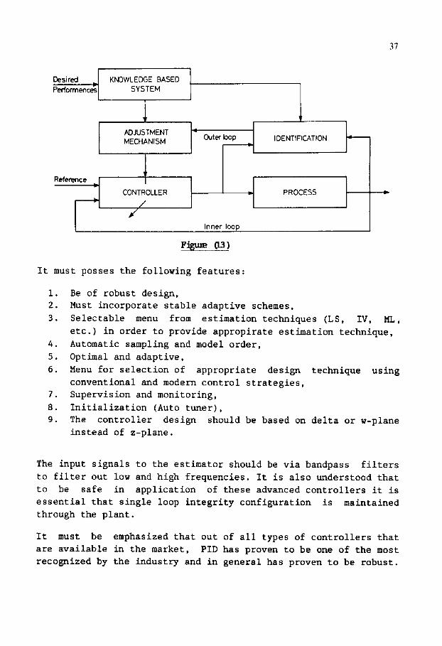
Combining features of autotuning and adaptation with supervision

and monitoring will result in the so called expert control[2]

(Figure 13). According to Astrom autotuners and adaptive

controllers can be viewed as a best tuning achieved by an able and

skilled instrument engineer. An expert control system automates

the capabilities of competent instrument and control engineers to

explore and reason about the selection of control strategies in

order to assess control performance.

Selection

The question often arises as to how to specify the controller

characteristics in order to achieve a desirable performance[5,30,

521.

Controller must be capable to switch over automatically from any

of the following modes in order to protect and provide complete

safety of the equipment for operation in the particular loop:

1. Manual,

2. Automatic,

3. Adaptive.

37

Desired J KNOWLEDGE BASED Peffon~ence~J ,, SYSTEM

Reference

-I

1 ADJUSTMENT MECHANISM

CONTROLLER /

/

[~" outer~p I -] IDENTIFICATION I- L

Inner loop

-1 ocEss I

F ~ 03)

It must posses the following features:

I. Be of robust design, 2. Must incorporate stable adaptive schemes,

3. Selectable menu from estimation techniques (LS, IV, ML,

etc.) in order to provide appropirate estimation technique,

4. Automatic sampling and model order,

5. Optimal and adaptive,

6. Menu for selection of appropriate design technique using

conventional and modern control strategies, 7. Supervision and monitoring,

8. Initialization (Auto tuner),

9. The controller design should be based on delta or w-plane instead of z-plane.

The input signals to the estimator should be via bandpass filters

to filter out low and high frequencies. It is also understood that

to be safe in application of these advanced controllers it is

essential that single loop integrity configuration is maintained through the plant.

It must be emphasized that out of all types of controllers that

are available in the market, PID has proven to be one of the most

recognized by the industry and in general has proven to be robust.

38

However the authors believe that the performance can be improved drastically by the applications of advanced control functions in terms of combining autotuning and advanced adaptive facilities.

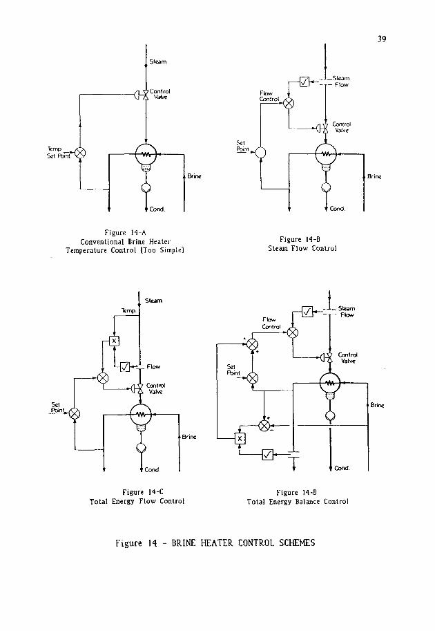
6. EFFICIENT CONTROL SCHEMES

The most important control loop in the desalination process that directly affect the production is the control of brine outlet temperature from the brine heater and in commonly referred to as top brine temperature. The efficiency of the brine heater depends on its being designed to meet the heat transfer requirements. The overall efficiency and performance of the desalination plant will depend on the type of control structure implemented. The existing brine heater control employed is very simple (Figure 14-A). This scheme has several shortcomings that are related to the way the disturbances affect the operation of the brine heater. Further enhancement could be achieved by incorporating brine heater pressure in the control scheme resulting in better performance,

fast response and short time delay. Optimal control of the brine heater can be accompolished by developing a state-space model or input-output model and using any suitable optimal/adaptive control

algorithm.

In order to reduce steam supply disturbances, a compensating flow loop will improve the response time (Figure 14-B). This scheme can further be enhanced by incorporating temperature measurement of the input steam resulting in energy control (Figure 14-C). In

this the temperature controller on the outlet of the brine heater adjusts the setpoint of the flow controller. This s theme

minimizes the disturbances in both the temperature and pressure of the input steam. This scheme shall especially be useful when the desalination plant is being fed from the back pressure or ext rat tion turbines.

The control scheme (Figure 14-C) can further be modified to incorporate total heat balance of the brine heater (Figure 14-D). This arrangement is certainly superior to the other schemes, since any disturbances in flow and temperature of the brine will be

39

Figure 14-A Conventional Brine Heater

Temperature Control (Too Simple)

Brine

Figure 14-C Total Energy Flow Control

Figure 14-B Steam Flow Control

Brine

Figure 14-D Total Energy Balance Control

Figure 14 - BRINE HEATER CONTROL SCHEMES

40

compensated by a corresponding change in the amount of input

energy to the brine heater.

The steam input disturbance causes subsequent variations of the temperatures and pressures in the cells and result in brine carry over.

To overcome these problems a control system can be designed that would make use of the anticipated temperatures change and

correspondingly activate the brine blowdown and make up flow control values in feed forward configuration.

A change in temperature, pressure or level of the first stage

brine affects the brine levels of all the succeeding cells. The best variable to be taken for the control is pressure of the first stage. This pressure change signal can be used for the make up control to maintain required level in the last stage cell.

7. CONCLUSION

The material presented in this paper is oriented toward modem

practitioner in the desalination field and generally valid for

other similar processes.

A brief description of

evaporator plants was

with Abu Dhabi settings.

control functions in multistage flash

presented with emphasis on the experience

Conventional controllers were discussed and the potential benefits of advanced digital control systems were highlighted including setpoint optimization. These include advanced control schemes. The application of these new methods in the desalination field is likely to result in a better understanding of the process dyanmics and thus enhance the control.

The use of high performance control systems is very desirable and

indeed strongly recommended. The use of a digital computers or microprocessors in the control loops offers numerous advantages

41

such as large choice of controller design strategies and

possibility to use more complex and efficient algorithms than the

simple PID normally employed. The implementation of advanced

control methods provide efficient process control, supervise plant

automation and ensure optimization of plant operation. The

application of a decentralized hierarchical control strategies

ensures the highest reliability and availability of the plant.

REFERENCES

II

21

31

41

51

61

71

81

91

Adrake, F.. “Measurements and Conlrol In Flash Evaporation Plants” Desallnatlon (1986) 241-262.

Elsevler Science Publishers B.V.. Amslerdam.

Astrom. K.J.. Anlon. J.J.. and Aezen K.E.. 119861. “Experl Conlrol”. Aulomallca. Vol. 22, No. 3.

pp. 277-286.

Astrom. K.J.. and Wlllenmark. B.. “Adal~llve Control”. Addison-Wesley. Readlna Mass., 1988.

Astrom. K.J.. “Theory and Applications of Adaptive Conlrol - A Survey”. Aulomallca Vol. 19. No.5.

pp. 471-486, 1983.

Astrom. K.J.. Haaglund. T.. “Aulomalic Tuning of Simple Regulalors wilh Speclllcatlons on Phase

and Amplitude Margins”. Aulomatlca. Vol. 20. No& pp. 645-651. 1984.

Astrom. K.J.. Wlllenmark. B.. “Computer Conlrolled System”. Prentice-Hall. Inc., 1984.

Aslrom. K.J., “Adaptive Feedback Conlrol”. Proceedings of the IEEE. Vo1.75. No.2. Feb. 1987.

Ball, S.J.. Clapp. Jr. N.E.. and Delene. J.G.. Oak Ridge Natlonal Laboralory. Tennessee.

“Nuclear Desallnallon Plant Conlrol Studies”. 4th lnlernatlonal Symposium on Fresh Waler from Sea.

Vol. 2. 429-438. 1983.

Barba. D.. Lluzzo. G.. and Tagllalfrrl. G.. “Malhematlcal Model for MultIflash Desalllng Plan1

Conlrol”. Cenlro Progellazlone Ollimaxlone Soclela Ilallana Reslne. Rome. 4111 lnternallonal

Symposium on Fresh Waler lrom Sea. Vol. I. 153-168. 1973.

IO] Clarke. D.W.. Gawlhrop. P.J.. “Self-Tuning Control”. Proc. IEE. Vol. 126, No.6. June 1979.

III Ch-Tsone Chen. “Linear System Theory and Design”, Holl-Saunders lnlernatlonal Edlllons.

I21

131

141

151

Carl. R.. Maflezzonl. C., “Pracllcal-Opllmal Conlrol of a Drum Boiler Power Plant”. Automallca.

Vol. 20. No. 2. pp. 163-173. 1984.

DuyfJes. G.. Van Der Grlnlen. P.M.E.M.. “Appllcallon of a Mathematical Model for Ihe Conlrol and

Opllmlzatlon of a Dlsilllallon Plant”. Automallca. Vol. 9. pp. 537-547. Pergamon Press. 1973.

El-Hares. H., “lnstrumentatlon Problems in Libyan Desallnatlon Planls”, Al Fateh University,

Tripoli.

El -Sale. M.H.A.. Ramadan. A.H.. and Gamma. S.S.. “Mulll-Stage Flash Desalination Process Control

Sysleol”. IFAC Workshop. Trlpoll. pp 87-98.

42

161 Edgar, T.F.. Hlmmelblau. D.M.. “Optlmtzatlon of Chemical Process”. McGraw-H111 lnternatlonal

Edltlons Chemical Englneerlng Series.

171 Farrag. M.F.. and Erfan. M.H., “Computer Supervisory Control of Mulll-Stage Flash Evaporators”. Dr. Sale. Consulting Engineers. Cairo.

181 Furukl. A.. Hamanaka. K.. Talsumoto. M.. and tnohara. 5.. “Aulomattc Control System of MSF Process” [ACSODE [RI], Mllsublshl Heavy Industries. Ltd.. Tokyo.

IS] Farelgh. D.M.K.. V.E.D. Abu Dhabl and Arazztnl. 5.. Desatlnallon Devlslcn. Itallmplanlt. Geneva. “Descrtpllon and Mathemallcal Model of a Large Desallnallon Plant In Scads Conflguratton”.

201 Flugge-Lotz. “The Importance of Opllmal Control for the Practical Engineer”. Automatlca. Vol. 6.

pp. 749-753. Pergamon Press, 1970.

21) Grelfath. R.. and Maylnger. F.. “A Conlrol System for Multl-Stage Flash Desalination Plants”,

lnstllut lur Verfahrenslechnik der Unlversltat Hannover. (G.F.R.).

221 George, A.R.. and Tyler, B.. “Control and lnstrumenlatlon Enpertence al LO& on PA1 MSF Sea Water

Desltnallon Plant”. Blnnle and Partners, London.

231 Glueck. A.R.. Lawrencevllle. New Jersey and Bradshaw. R.W.. Stanlord Unlverslty, California. “A

Malhematlcal Model for Multt-slage Flash Dlstlllatlon Planl”, 3rd lnternallonal Symposium In Fresh

Water from Sea. Vol.1. 95-108. 1970.

241 Grlmble. M.J.. “Recent Trends inthe Design of MultIvariable Control Syslems” by Optlmal Melhods.

24a] Grlmble. M.J.. Johnson. M.A.. “Optlmal Control and Slochastlc Estlmatlon: Theory and Appllcallons

Volume I & Volume 2”, A Wiley-lntersclence Publtcatlon. John Wiley & Sons.

251 Gene FrankIln. F.. David Powell. I., Michael Workman, L., “Dlgltal Control of Dynamic Syslems”.

Addison-Wesley Publlshlng Company.

261 Hultln. G.O.. and Harper, R.. “Desallnalton Plant Control with Mlcroprocessor Based Dlgllal

Technology”. Desalination. 45 (19831 329-336. Elsevler Science Publishers B.V.. Amsterdam.

271 Helal. A.M., Medanl. M.S.. and Sollman. M.A.. “A Tradltlonal Malrlx Model for Mulll-Stage Flash DesallnaIlon Planls”. Computers and Chemical Englneerlng. Vol. ID No. 4. ~~327-342. 1986.

281 Hayakawa. K.. Satorl. H.. and Konlshl. K.. IHI Lid.. Tokyo “Process Slmulalton on a Mulll-Stage

Flash Dlsllllallon PlanI”. 4lh Internalloml Symposium on Fresh Water from Sea. Vol. 1. 303-312.

1973.

29) Harmony Ray, UT.. ‘*Advanced Process Conlrol”, Bulterworths Reprint Series In Chemical Englneerlng

1989.

301 Hagglund. T.. Aslrom. KJ.. “An lnduslrlal Adapllve PID Controller”. Sal1 Control Instruments AB

and Lund lnslltule of Technology, Lund, Sweden.

311 lnduslrlal Dlgltal Control Systems, Edlled by Wsrwlck. K.. and Rees. D.. Peter Peregrlnur Lld. 1988.

321 lmplemenlallon d Self-Tuning Controllers. Edlted by Kevin Varwlck. Peter Peregrlnus Ltd., 1988.

331 Johnson, A.. “Duallly of the Discrete-Time Optlmat Filler and Regulator Problems”. IEE

Proceedings. Vol.130. PI. D. No. 4. July 1983.

341 Johnson, A., “Process Dynamics Estlmaticm and Conlrol”. Peler Peregrlnus Lid.. London, U.K. 1985.

351 John D’Azoo, J.. Conslanllne Houpls, H., “Linear Control System Analysis and Design”. ConventIonal

& Moder. lnternrllonal Sludenl Edltlon, 1981.

361 Kershenbaum. L.S.. Forlescue. T.R., “lmplemenlalion of on-line Control In Chemical Process

P lanls”. Automallca. Vol. 17. No. 6. pp. 777-788. 1981.

43

371 Kuceta, V.. “Dlscrele Linear Conlrol: The Pclynomlal Equatlon Approach”. Wiley. Chichester, U.K.,

1979.

381 Lennarl LJung. and Torslen Soderslrom. “Theory and Pracllce of Recursive Identlflcatlon”. The MIT

Press Cambrldge. Massachusetts. London, England, 1986.

38a] Lelghl. J.R.. “Applled DIgital Control; Theory, Design and Implemenlatlon”. Aprentlce-Hull

Inlernatlonal. Englworeds Cliffs. New Jersey, 1985.

39) Mannesmann. Hartmann Er Braun. Protronlc P. Dlgltric P. Slate Controller wlth Observer.

401 Mlyazuka. 5.. Klshlmolo. H., Shloya. H.. Nakamura. H., “Advanced Control Optlmal RegUlatOr

for Dlstrlbuled Control Syslems (ACORD)“. Bailey Japan Co. Ltd.

411 Mahmoud, M.S., and Slngh, M.G.. “Discrete Systems Analysis. Control and Opllmlzatlon” Springer-

Verlag. 1984.

421 Nakamura. H., “Advanced Control for Thermal Power Planls Applied Systems”. Bailey Japan Co., Lld.

431 Paul W. Murrlll, “Fundamen;als of Process Conlrol Theory”. An Independent Learnlng Module from lhe

Instrument Soclely of America. 1981.

441 Pradeep Deshpande, B.. Raymond Ash, H.. “EleIIIentS of Computer Process Control wllh Advanced

Control Appltcallons”, Instrument Soclely of America. 1981.

451 Peter Young, “Recursive Estlmallon and Time-Series Analysis” An Introducllon. Springer-Verlag.

New York, 1984.

46) Rebagllall. S., Ghlarza. E., and Abuelda. K.S.. “One Year Operatlon Experience on the Process

Control System and UANE MSF Desallnallon Plant” Desallnatlon 75, Elsevler Science PublIsherr.

B.V.. Amsterdam.

471 Sebor6. D.E.. Edgar, T.F.. Shah, S.L.. “Adapllve Control Strategies for Process Conlrol : A

Survey AICHE Journal”, June 1986. Vol. 32. No. 6.

481 Singh. M.G.. and Tltll. A.. “Systems Decomposllion. Optlmlzallon and ConIrol”. Pergeman

lnternatlonal Llbrary. 1978.

491 Shlnskey. F.G.. “Process Control Systems”, McGraw-HI11 Publishing Company, 1988.

501 Soderslron. T.. and Slolca. P.. “System Identlflcatlon”, Herlfordshlre. U.K., Prentice Hall

Internallonal, 1989.

511 Spllelhoff, H.. Klefenz. G., Nlcoial, W., Traulmann. G.. “Experience and Resull wllh the State

Controller for the Live Sleam Temperature Conlrol of a 2250 t/h Steam Generalor” Mannesmann

Harlmann and Braun.

521 Tore Ha66lUnd. “Adapllve PID Control”. ICHEME - Advances In Process Control II. Salt Conlrol

Inslruments AB. Lund, Sweden, pp.177-184. 1988.

53) Unbehauen. H., and Rao. G.P.. “ldenllflcallon of Conllnuous Systems”. North-Holland. Amsterdam.

ISBN D-444-70316-0.

541 Wladyslaw Flndelsen. Mleczyslaw Bryds. Krzyszlof Mallnowskl. Plolr TatJewskl. and Adam Womlak.

“On-Line Hlerarchlcal Control for Sleady-State Systems”. IEEE Transacltons on Automatic Control,

Vol. AC-23, No.2. pp. 189-207. April 1978.