Desalination,74 (1989) 317-326 Elsevier Science Publishers B.V., Amsterdam - Printed in The Netherlands

317

SIMULATION OF MSF DESALINATION PLANTS

I.S. Al-Mutaz and M.A. Soliman

Chemical Engineering Department, King Saud University, P.O.Box 800, Riyadh 11421, Saudi Arabia

ABSTRACT

A very fast steady state simulation method is presented for MSF desalina-

tion plants based on the method of orthogonal collocation. Instead of solving

mass and heat balances for all stages very few selected stages are solved. The

selected stages are chosen to be at the roots of a suitable orthogonal polyno-

mial.

Calculations show that. the method is remarkably efficient and at. least

twice faster than a method based on the simultaneous solution of all stages

mass and heat balances.

INTRODUCTION

The Arabian Gulf countries have about 60% of the total world desalting

capacity. About 67.6% of the total capacity installed are of the multi-stage

flash (MSF) type. Moreover, the MSF plants account for over 84% of the large

size plants erected so far.

The simulation of MSF plant provides the ability to optimize designs and to

predict performance of a plant under the intended operating conditions. It can

save much time and money when operating policies had to be altered. Almost all

previous MSF simulation are based on solving the numerous, nonlinear and

complex mass and heat balances equations by stage to stage calculations. This

method suffers from the instability and low rate of convergence.

A great deal of MSF simulations have been done by assuming constant physi-

cal properties, heat transfer coefficients and temperature drop in each stage

(l-4). Other simulation studies have been done to reduce the number of equa-

tions to be solved. Soliman (5) has relaxed the assumptions by giving them

different. values in different sections of the plants. Barba et al (6) have

further relaxed these assumptions and obtained a model that required iterative

solution.

OOll-9164/89/$03.50 0 Else&r Science Publishers B.V.

318

Other works have been carried toward the minimization of the iterative

calculation obtained by the stage to stage computation, either by optimization

(7), stage-wise calculation (8) or loopnest model (9).

In the present work, few selected stages of the MSF plant have been used to

simulate the plant performance. The orthogonal collection method has been used

to solve the steady state operation of MSF plant.

MSF DESALINATION PROCESS

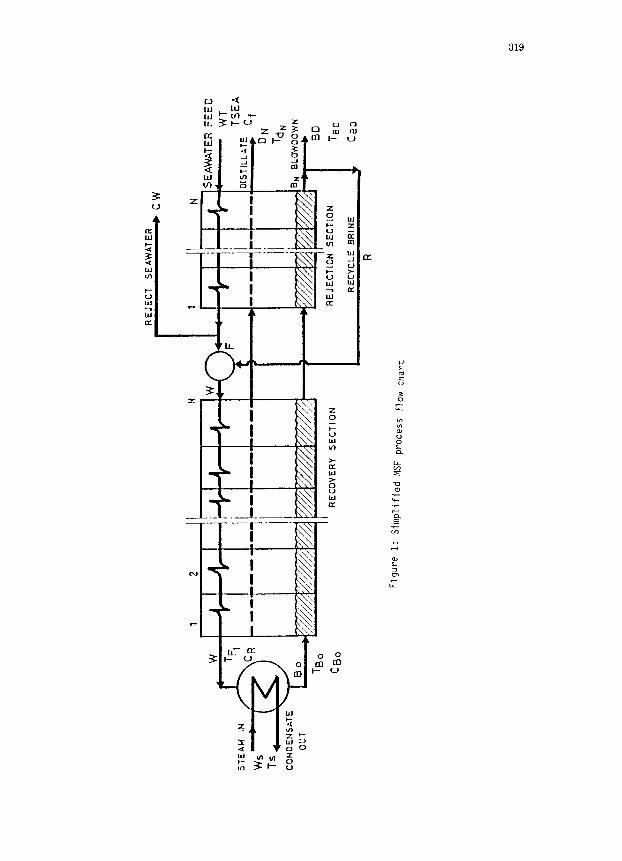
Figure 1 shows the MSF process which has three distinct sections; heat

rejection section, heat recovery section and brine heater. The feed water, WT,

passes through the heat rejection and heat recovery sections.

On leaving the first (warmest) rejection stage the feed stream is split

into two parts, reject seawater CW which passes back to the sea and a make up

stream F which is then combined with the recycle stream R. The combined stream

W now passes through a series of heat exchangers, its temperature rising as it

proceeds towards the heat input section of the plant. Passing through the

brine heater the brine temperature is raised from TFI at the inlet of the brine

heater to a maximum value TUo approximately equal to the saturation temperature

at the system pressure.

The brine then enters the first heat recovery stage through an orifice thus

reducing the pressure. As the brine was already at its saturation temperature

for a higher pressure, it will become superheated and flashes to give off water

vapour. This vapour passes through a wire mesh (demister) to remove any entrai-

ned brine droplets and onto a heat exchanger (as shown in the figure) where the

vapour is condensed and drips into a distillate tray. The process is then

repeated all the way down the plant as both brine and distillate enter the next

stage which is at a lower pressure. The concentrated brine is divided into two

parts as it leaves the plant, the blow-down BD which is pumped back to the sea

and a recycle stream R which returns to mix with the make up stream F.

THE SIMULATION MODEL AND PROCEDURE

Figure 2 represents the temperature notation in stage j in the rejection or

the recovery sections, while Figure 3 shows locations of the selected points.

SEA

WA

TER

FE

ED

COND

ENSA

TE

Ca0

’ RE

COVE

RY

SECT

ION

REJE

CTIO

N SE

CTIO

N T5

0

RECY

CLE

BRIN

E 9

Cao

R

Figu

re 1:

Si

mpli

fied

MS

F pr

oces

s fl

ow ch

art

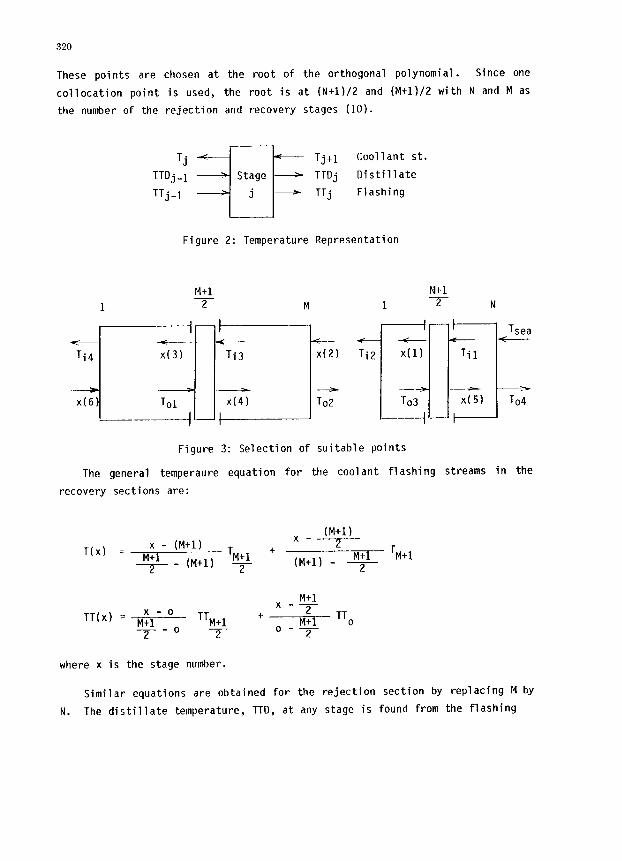
These points are chosen at the root of the orthogonal polynomial. Since one

collocation point is used, the root is at (N+l)/Z and (M+l)/Z with N and M as

the number of the rejection and recovery stages (10).

Tj TTDj_1

TTj-1

Coollant st.

Distillate

Flashing

Figure 2: Temperature Representation

M+l 2

N+l 1 2 N

Figure 3: Selection of suitable points

The general temperaure equation for the coolant flashing streams in the

recovery sections are:

T(x) = x - (M+l)

+ _ (M+l) ‘y +

x_M+l TT(x) = M;l- ' TTM+l

2

--0 2 2

+ o _ M+1 TT~

2

where x is the stage number.

Similar equations are obtained for the rejection section by replacing M by

N. The distillate temperature, TTD, at any stage is found from the flashing

321

temperature after subtracting the boiling point elevation, so

TTD(j) = TT(j) - Zj

where Zj is called the thermal resistance. It contains the boiling point ele-

vation and the non-equilibrium allowance.

The model calculation is started by assuming initial values of the X

variables shown in Figure 3. For MSF plant with known number of stages, the

following temperatures are calculated

TiI = N_l X(1) + 2 Tsea N+l N+l

Ti2 = 2N X(1) - N_l Tsea N+l N+l

Ti3 =M_l X(31 + __J___ X(21 M+l M+l

Ti4 =2M X(3) -M_l X(2) M+l M+l

To1 = M-l X(4) +A X(6) M+l M+l

To2 =a X(4) -M-l XI6) M+l M+l

To3 =N-l X(5) +__?__ To2 N+l N+l

To4 = c X(5) - _!-L To2 N+l N+l

Also define the following variables

Bwtl = X(8)

bwt2 = N-l X(81 + ._?_._ bwt6 N+l N+l

bwt3 = X(7)

bwt4 = M-l X(7) + ._._?__ M+l M+l

322

bwt5 = ~ 2 N X(8) - N-1 bwt6 _ N+l N+l

bwt6 = x X(7) - M-l M+l M+l

rl = wtl/wt

r2 = wrc/wt

r3 = wrj/wt

dwtj = 1 - bwtj

where, wt is the coolant flow rate in the recovery section

wtl is the coolant flow rate in the rejection section.

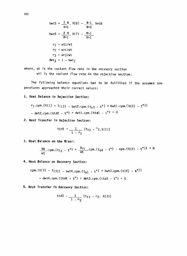
The following balance equations had to be fulfilled if the assumed tern.

peratures approached their correct values:

1. Heat Balance in Rejection Section:

rl.cPm.(X(l) - til)) - bwt2.cpm.(to3 _ t*) + bwtl.cpm.CX(5)

- dwt2.cpm.(ttd2 - t") + dwtl.cpm.(ttdl - t*) = o

2. Heat Transfer in Rejection Section:

ttdl = __._L_ (til - "1.X(l)) 1 -"I

3. Heat Balance on the Mixer:

‘m -Cplll.( tjz - t*) + Wt- -- wrc cpm.(t,4 _ t*) - cpm.(X(Z) - t*)) = 0

Wt

4. Heat Balance on Recovery Section:

cpilL(X(3) - ti3)) - bwt4.cpm.(tol _ t*) + bwt3.cpm.(X(4) - t*))

- dwt4.cpm.(ttd4 - t*) + dwt3.cpm.(ttd3 - t*) = 0

5. Heat Transfer in Recovery Section:

ttd3 - 1 (ti3 - "2. X(3)) 1 -"2

323

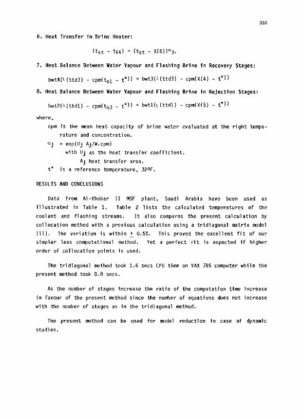
6. Heat Transfer in Brine Heater:

(tst - ti4) = (tst - X(6))a3.

7. Heat Balance Between Water Vapour and Flashing Brine in Recovery Stages:

bwt4(X(ttd3) - cpm(t,l - t*)) = bwt3(h(ttd3) - cpm(X(4) - t*))

8. Heat Balance Between Water Vapour and Flashing Brine in Rejection Stages:

bwt2(x(ttdl) - Cpm(t,3 _ t*)) = bwtl(~(ttdl) - CPidX(5) - t*))

where,

cpm is the mean heat capacity of brine water evaluated at the right tempe-

rature and concentration.

ci* J = exp(Uj Aj/W.cpm)

with Uj as the heat transfer coefficient.

Aj heat transfer area.

t* is a reference temperature, 320F.

RESULTS AND CONCLUSIONS

Data from Al-Khobar II MSF plant, Saudi Arabia have been used as

illustrated in Table 1. Table 2 lists the calculated temperatures of the

coolant and flashing streams. It also compares the present calculation by

collocation method with a previous calculation using a tridiagonal matrix model

(11). The variation is within + 0.5%. This proved the excellent fit of our - simpler less computational method. Yet a perfect iit is expected if higher

order of collocation points is used.

The tridiagonal method took 1.6 sets CPU time on VAX 785 computer while the

present method took 0.8 sets.

As the number of stages increase the ratio of the computation time increase

in favour of the present method since the number of equations does not increase

with the number of stages as in the tridiagonal method.

The present method can be used for model reduction in case of dynamic

studies.

324

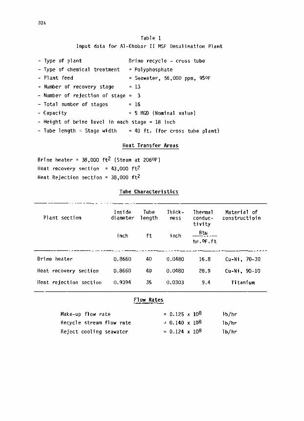
Table 1

Input data for Al-Khobar II MSF Desalination Plant

Type of plant Rrine recycle - cross tube

Type of chemical treatment = Polyphosphate

Plant feed = Seawater, 56,000 ppm, 950F

Number of recovery stage = 13

Number of rejection of stage = 3

Total number of stages = 16

Capacity = 5 MGD (Nominal value)

Height of brine level in each stage = 18 inch

Tube length = Stage width = 40 ft. (for cross tube plant)

Heat Transfer Areas

Brine heater = 38,000 ft.* (Steam at 206oF)

Heat recovery section = 43,000 ft2

Heat Rejection section = 38,000 ft2

Tube Characteristics

Plant section Inside Tube Thick- Thermal Material of

diameter length ness conduc- constructioin tivity

inch ft inch Btu

hr.oF.ft

Brine heater 0.8660 40 0.0480 16.8 Cu-Ni, 70-30

Heat recovery section 0.8660 40 0.0480 28.9 Cu-Ni, 90-10

Heat rejection section 0.9394 35 0.0303 9.4 Titanium

Flow Rates

Make-up flow rate

Recycle stream flow rate

Reject cooling seawater

= 0.125 x 108 lb/hr

= 0.140 x 108 lb/hr

= 0.124 x 108 lb/hr

325

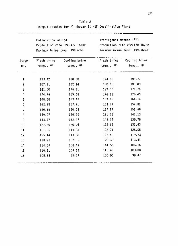
Table 2

Output Results for Al-Khobar II MSF Desalination Plant

Collocation method Tridiagonal method (11)

Production rate 2229477 lb/hr Production rate 2221470 lb/he

Maximum brine temp. 199.63OF Maximum brine temp. 199.7680F

Stage Flash brine Cooling brine Flash brine Cooling brine

No. temp., oF temp., oF temp., oF temp., oF

1 193.42 188.38 194.05 188.77

2 187.21 182.14 188.95 183.03

3 181.00 175.91 182.30 176.75

4 174.79 169.68 176.11 170.45

5 168.58 163.45 169.95 164.14

6 162.38 157.21 163.77 157.81

7 156.18 150.98 157.57 151.48

8 149.97 149.79 151.36 145.13

9 143.77 132.27 145.14 138.78

10 137.56 126.04 138.93 132.43

11 131.35 119.81 132.71 126.08

12 125.14 113.58 126.50 119.73

13 118.93 107.35 120.30 113.41

14 114.57 108.49 114.55 108.16

15 110.21 104.35 110.43 103.88

16 105.85 99.17 106.96 99.47

326

REFERENCES

l- Spiegler, K.S., "Principles of Desalination", Academic Press, N.Y. (1966).

2- Mandil, M.A. and Abdel Ghafour, E.E., Chem. Eng. Sci., 25, 611-621 (19701.

3. Howe, E.D., "Fundamentals of Desalination", N.Y., Marcel Dekker, Inc., N.Y.

(1974).

4. Toyama, S., “Optimization of MSF Process Design", 3rd Int. Symp. on Fresh

Water from the Sea, Vol. 1, p. 219 (1970).

5. Soliman, M.A., J. of Eng. Sci., Univ. of Riyadh, Vol. 7, No. 2 (1981).

6. Barba, O., Linzzo, G. and Tagliferri,G., "Mathematical Model for Multiflash

Desalting Plant Control", 4th Int. Symp. on Fresh Water from the Sea, Vol.

1, 153-168 (1973).

7- Beamer, J.H. and Wilde, D.J., Desalination, 2, 259-275 (1971).

8- Rautenbach, R. and Buchel, H.G., "Modular Program for Design and Simulation

of Desalination Plants", Proceeding of the 7th Int. Symp. on Fresh Water

from the Sea, Vol.1, 145-161 (1980).

9- A.M. Omar, "Simulation of Multistage Flash Desalination Plants", An M.Sc.

Thesis, UPM, Dhahran, Saudi Arabia, Sept., 1981.

lo- W.E. Stewart, K.L. Levien and M.Porari, "Simulation of Fractionation by

Orthogonal Collocation", Chemical Engineering Sciences, 40(3), 409 (1985).

ll- A.M. Helal, M.S. Medani, M.A. Soliman and J.R. Flower, "A Tridiagonal Mat-

rix Model for Multistage Flash Desalination Plants", Computers and Chemical

Engineering, Vol. 10, No. 4, 327 (1986).