dynamic simulation of brown stock washers and bleach plants
128
DYNAMIC SIMULATION OF BROWN STOCK WASHERS AND BLEACH PLANTS by Roseanne Xiaohong Wang M.Eng. General Research Institute for Non-Ferrous Metals, China, 1987. A THESIS SUBMITTE D IN PARTIAL FULFILLMENT OF THE REQUIREMENTS FOR THE DEGREE OF MASTER OF APPLIED SCIENCE in THE FACULTY OF GRADUATE STUDIES DEPARTMENT OF CHEMICAL ENGINEERING We accept this thesis as conforming to the required standard THE UNIVERSITY OF BRITISH COLUMBIA July, 1993 © Roseanne Xiaohong Wang, 1993
-
Upload
khangminh22 -
Category
Documents
-
view
1 -
download
0
Transcript of dynamic simulation of brown stock washers and bleach plants

DYNAMIC SIMULATION OF BROWN STOCK WASHERS AND BLEACH PLANTS
by Roseanne Xiaohong Wang
M.Eng. General Research Institute for Non-Ferrous Metals, China, 1987.
A THESIS SUBMITTED IN PARTIAL FULFILLMENT OF
THE REQUIREMENTS FOR THE DEGREE OF
MASTER OF APPLIED SCIENCE
in
THE FACULTY OF GRADUATE STUDIES
DEPARTMENT OF CHEMICAL ENGINEERING
We accept this thesis as conforming
to the required standard
THE UNIVERSITY OF BRITISH COLUMBIA
July, 1993
© Roseanne Xiaohong Wang, 1993
In presenting this thesis in partial fulfilment of the requirements for an advanced
degree at the University of British Columbia, I agree that the Library shall make it
freely available for reference and study. I further agree that permission for extensive
copying of this thesis for scholarly purposes may be granted by the head of my
department or by his or her representatives. It is understood that copying or
publication of this thesis for financial gain shall not be allowed without my written
permission.
(Signature)
Department of ^ce4.19
The University of British ColumbiaVancouver, Canada
Date^479
DE-6 (2/88)
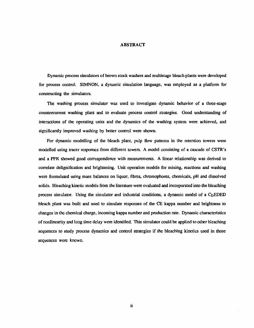
ABSTRACT
Dynamic process simulators of brown stock washers and multistage bleach plants were developed
for process control. SIMNON, a dynamic simulation language, was employed as a platform for
constructing the simulators.
The washing process simulator was used to investigate dynamic behavior of a three-stage
countercurrent washing plant and to evaluate process control strategies. Good understanding of
interactions of the operating units and the dynamics of the washing system were achieved, and
significantly improved washing by better control were shown.
For dynamic modelling of the bleach plant, pulp flow patterns in the retention towers were
modelled using tracer responses from different towers. A model consisting of a cascade of CSTR's
and a PFR showed good correspondence with measurements. A linear relationship was derived to
correlate delignification and brightening. Unit operation models for mixing, reactions and washing
were formulated using mass balances on liquor, fibres, chromophores, chemicals, pH and dissolved
solids. Bleaching kinetic models from the literature were evaluated and incorporated into the bleaching
process simulator. Using the simulator and industrial conditions, a dynamic model of a CDEDED
bleach plant was built and used to simulate responses of the CE kappa number and brightness to
changes in the chemical charge, incoming kappa number and production rate. Dynamic characteristics
of nonlinearity and long time delay were identified. This simulator could be applied to other bleaching
sequences to study process dynamics and control strategies if the bleaching kinetics used in those
sequences were known.
11
TABLE OF CONTENTS
ABSTRACT^ ii
LIST OF TABLES^ vi
LIST OF FIGURES ^ vii
NOMENCLATURE ^ xi
ACKNOWLEDGMENTS ^ xv
DEDICATION ^ xvi
1 GENERAL INTRODUCTION^ 1
2 MODELLING, SIMULATION AND CONTROL OF BROWN STOCK WASHERS^5
2.1 Introduction^ 5
2.2 Process Description ^ 6
2.3 Model Development ^ 7
23.1 Introduction ^ 7
2.3.2 Process Variables and Analysis ^ 7
2.3.3 Modeling of Seal Tank ^ 9
2.3.4 Modeling of Drum Filter ^ 11
2.3.4.1 Mechanistic Approach^ 11
Mat Formation^ 12
Dewatering and Displacement Washing^ 12
2.3.4.2 Efficiency Approach ^ 15
2.3.5 Washing Stage and Plant Models ^ 16
2.4 Simulation of Process Dynamic Behavior ^ 18
2.4.2 A Single Washer ^ 18
2.4.3 Three Washers in Series ^ 19
111

2.5 Control Strategy Evaluation^ 25
2.5.1 Washing Process Control ^ 25
2.5.2 Results and Discussion ^ 28
2.6 Conclusions ^ 34
2.7 Recommendations and Suggestions for Future Work ^ 34
3 MODELING AND SIMULATION OF A BLEACH PLANT^ 37
3.1 Introduction^ 37
3.2 Process Description ^ 38
3.3 Model Development ^ 40
33.1 Process Variables and Analysis ^ 40
33.2 Modeling Flow Patterns in Retention Towers ^ 43
33.2.1 Introduction ^ 43
3.3.2.2 Observations and Models^ 43
3.3.3 Kinetic Models ^ 54
3.3.3.1 Introduction ^ 54
3.3.3.2 Chlorine Delignification^ 59
333.3 First Alkaline Extraction ^ 61
3.3.3.4 Chlorine Dioxide Bleaching ^ 66
33.3.5 Second Alkaline Extraction ^ 68
3.3.4 Correlation of Light Absorption Coefficient with Kappa Number after the Ei
Stage ^ 69
33.5 Mathematical Models of Unit Operations ^ 72
3.3.5.1 Mixer ^ 73
33.5.2 Tower ^ 74
CSTR (Continuous Stirred Tank Reactor)^ 75
PFR (Plug Flow Reactor)^ 76
33.5.3 Washer ^ 77
33.6 CDEDED Plant Model^ 77
iv
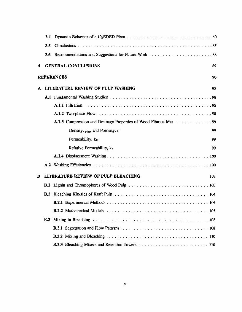
3.4 Dynamic Behavior of a CDEDED Plant ^ 80
3.5 Conclusions ^ 85
3.6 Recommendations and Suggestions for Future Work ^ 88
4 GENERAL CONCLUSIONS^ 89
REFERENCES^ 90
A LITERATURE REVIEW OF PULP WASHING^ 98
A.1 Fundamental Washing Studies ^ 98
A.1.1 Filtration ^ 98
A.1.2 Two-phase Flow^ 98
A.1.3 Compression and Drainage Properties of Wood Fibrous Mat ^ 99
Density, pm, and Porosity, c^ 99
Permeability, kp^ 99
Relative Permeability, kr^ 99
A.1.4 Displacement Washing^ 100
A.2 Washing Efficiencies ^ 100
B LITERATURE REVIEW OF PULP BLEACHING^ 103
B.1 Lignin and Chromophores of Wood Pulp ^ 103
B.2 Bleaching Kinetics of Kraft Pulp ^ 104
B.2.1 Experimental Methods ^ 104
B.2.2 Mathematical Models ^ 105
B.3 Mixing in Bleaching ^ 108
B.3.1 Segregation and Flow Patterns^ 108
B.3.2 Mixing and Bleaching ^ 110
B.3.3 Bleaching Mixers and Retention Towers ^ 110
LIST OF TABLES
2.1 Mathematical model of a washing stage^ 17
22 Operating data of an industrial vacuum drum washing plant ^ 19
2.3 Mean and variance of dissolved solids carryover resulting from three control strategies. . . ^ 32
3.4 Results from fitting CSTRS+PFR and CSTRS models to tracer experimental data. ^ 49
3.5 Experimental conditions used in bleaching kinetics studies for different bleaching stages. . . ^ 60
3.6 Kinetic data base for alkaline extraction of chlorine bleached Kraft pulps^ 62
3.7 Kinetic data base of alkaline extraction for chlorine dioxide bleached Kraft pulps ^ 64
3.8 Comparison between our modified model and Axegird model^ 66
3.9 Rate constants A1 and A2 for C102 bleaching for different pulps^ 67
3.10 Stoichiometric constants n and A3 for C102 consumption in C102 bleaching for
different pulps^ 68
3.11 Data base of brightness versus kappa number after the first extraction stage and light
absorption coefficient calculated using Kubelka-Munk equation. ^ 71
3.12 Operating conditions of a CDEDED bleach plant. ^ 80
3.13 Input data for simulation of a CDEDED bleach plant ^ 81
3.14 Comparison between predicted and experimental data at steady state after retention
towers of a CDEDED bleach plant ^ 82
B.15 Relative reaction/mixing rates for common pulp mixers^ 111
vi
LIST OF FIGURES
1.1 Kraft pulp process schematic. ^ 2
2.2 Flow diagram of a three-stage vacuum drum washing plant. ^ 6
2.3 Schematic diagram of a vacuum drum washing stage. ^ 8
2.4 Comparison of flow pattern models for a seal tank.^ 10
2.5 Operating zones in a drum filter. ^ 11
2.6 Simulation model structure for a three-stage washing plant. ^ 17
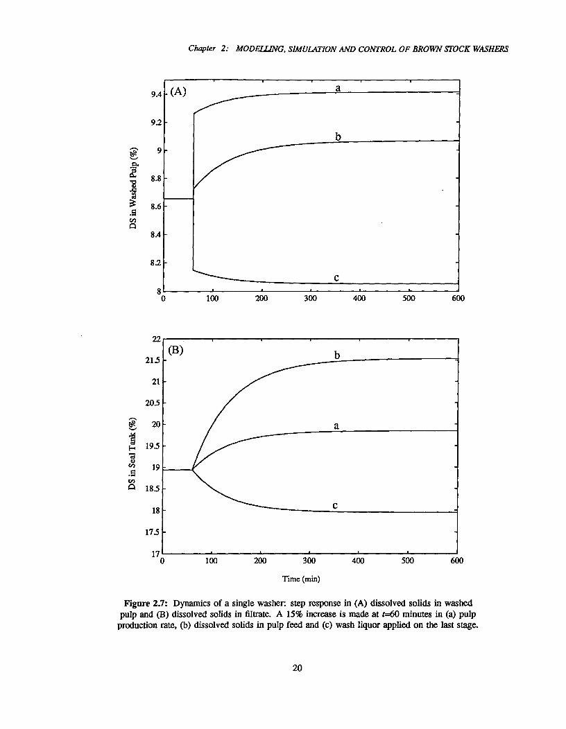
2.7 Dynamics of a single washer: step response in (A) dissolved solids in washed pulp and (B)
dissolved solids in filtrate. A 15% increase is made at t=60 minutes in (a) pulp production
rate, (b) dissolved solids in pulp feed and (c) wash liquor applied on the last stage 20
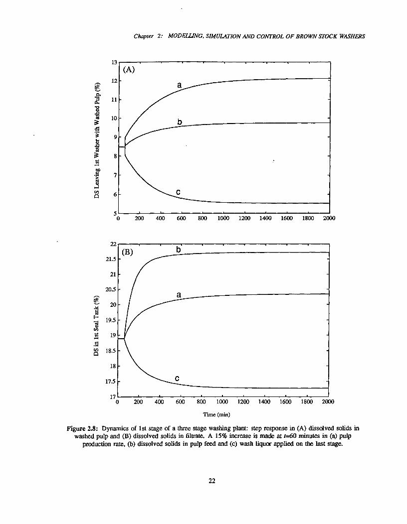
2.8 Dynamics of 1st stage of a three stage washing plant: step response in (A) dissolved
solids in washed pulp and (B) dissolved solids in filtrate. A 15% increase is made at
t=60 minutes in (a) pulp production rate, (b) dissolved solids in pulp feed and (c) wash
liquor applied on the last stage. ^ 22
2.9 Dynamics of 2nd stage of the three stage washing plant: step response in (A) dissolved
solids in washed pulp and (B) dissolved solids in filtrate. A 15% increase is made at
t=60 minutes in (a) pulp production rate, (b) dissolved solids in pulp feed and (c) wash
liquor applied on the last stage. ^ 23
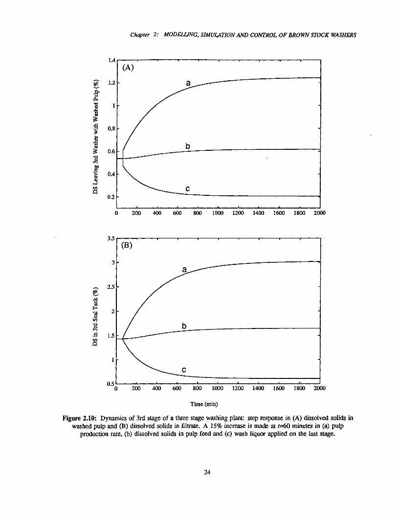
2.10 Dynamics of 3rd stage of a three stage washing plant: step response in (A) dissolved
solids in washed pulp and (B) dissolved solids in filtrate. A 15% increase is made at
t=60 minutes in (a) pulp production rate, (b) dissolved solids in pulp feed and (c) wash
liquor applied on the last stage 24
vii

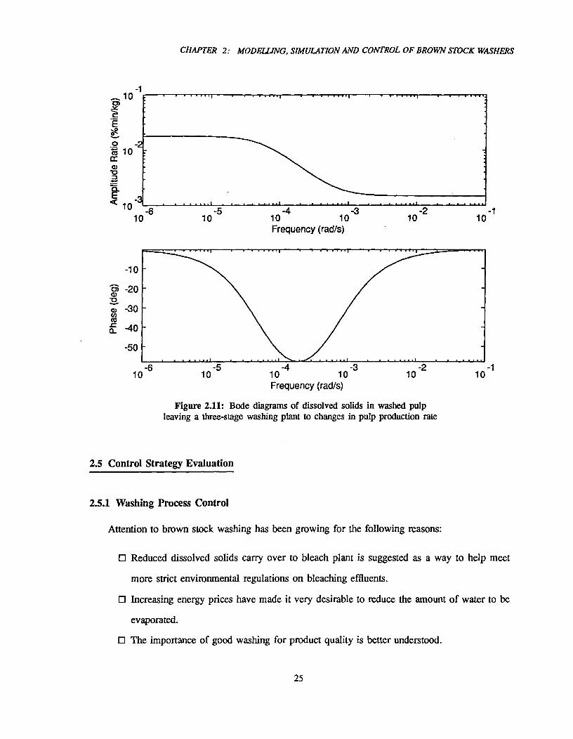
2.11 Bode diagrams of dissolved solids in washed pulp leaving a three-stage washing plant
to changes in pulp production rate ^ 25
2.12 Bode diagrams of dissolved solids in washed pulp leaving a three-stage washing plant
to changes in wash liquor flow rate ^ 26
2.13 Control layout of a three-stage vacuum drum washing plant. ^ 29
2.14 Process disturbances used in simulation of control strategies for a three-stage washing
plant: fluctuations in (A) dissolved solids content in pulp feed and (B) pulp production
rate. 30
2.15 Dissolved solids carryover of a three-stage washing plant using different control
strategies^ 31
2.16 Liquor levels in three seal tanks under proportional control (Strategy 3 example). ^ 33
2.17 Effects of anti-windup on control performance. ^ 35
3.18 Process flow diagram of a CDEDED bleach plant. ^ 39
3.19 Process units and variables of a bleach stage. ^ 41
3.20 Typical RTD in a low consistency tower^ 46
321 Typical RTD in a medium consistency tower. ^ 47
322 Flow patterns, plots of associated residence time distributions and tracer responses for
an upflow tower^ 48
3.23 Measured residence time distribution and model predictions for an upflow C tower
with bottom and mid circulators in operation. ^ 50
3.24 Measured residence time distribution and model predictions for an upflow C tower
with a bottom circulator in operation. ^ 51
3.25 Measured residence time distribution and model predictions for a C tower. ^ 51
326 Measured residence time distribution and model predictions for a downflow El tower. . . ^ 52
VIII

3.27 Measured residence time distribution and model predictions for an upflow DI tower. . . . 52
3.28 Measured residence time distribution and model predictions for a downflow E2 tower. . . . 53
3.29 Measured residence time distribution and model predictions for an upflow D2 tower. . . . 53
3.30 Three sequences of a CSTRS+PFR model with two CSTR's. 54
3.31 Comparison between CSTRS+PFR and PFR model responses of residual chlorine to a
step change in inlet kappa number. ^ 55
3.32 Comparison between CSTRS+PFR and PFR model responses of residual chlorine to a
step change in chlorine charge. ^ 55
3.33 Comparison between CSTRS+PFR and PFR model responses of kappa number after C
tower to a step change in inlet kappa number.^ 56
3.34 Comparison between CSTRS+PFR and PFR model responses of kappa number after C
tower to a step change in chlorine charge^ 56
3.35 Difference between CSTRS+PFR and PFR models responses of residual chlorine
dioxide to a step change in chlorine dioxide charge. ^ 57
3.36 Difference between CSTRS+PFR and PFR model responses of brightness after DI
tower to a step change in chlorine dioxide charge. ^ 57
3.37 Comparison between CSTRS+PFR and PFR model predictions of residual chlorine
dioxide as a function of chlorine dioxide charge^ 58
3.38 Comparison between CSTRS+PFR and PFR model prediction of brightness after D1
tower as a function of chlorine dioxide charge ^58
3.39 Kappa number during El bleaching of chlorine bleached pulps as calculated by our
modified model and Axegard's model^ 65
3.40 Kappa number during El bleaching of a chlorine dioxide bleached pulp as calculated
by our modified model and Axegfird's model. ^ 67
3.41 Light absorption coefficient vs. kappa number after first extraction stage^ 72
ix

3.42 Block diagram of a bleaching unit operation model: mixer^ 73
3.43 Block diagram of a bleaching unit operation model: reactor. ^ 75
3.44 Block diagram of a bleaching unit operation model: washer. ^ 77
3.45 Flowsheet of a typical CDEDED bleach plant and corresponding simulation block
diagram. ^ 78
3.46 CDEDED bleach plant response to step changes in total available chlorine charge in CD
stage. ^ 83
3.47 CDEDED bleach plant response to typical variations in incoming kappa number.^ 84
3.48 CDEDED bleach plant response to a step change in pulp production rate^ 86
A.49 A generalized washing system described by Norden model. ^ 101
^
B.50 An example of bleaching reaction characteristics 108
x

NOMENCLATURE
Ai^ Constant in Equation 3.39, kg2,m-4,
A2^ Constant in Equation 3.39, kg2/m4A3^ Constant in Equation 3.40, m2"/Icgn-1a^Coefficient in Equation 3.46, kg/m2
am^Specific resistance of mat, m/kg
Constant in Equation 3.46, m2/kgBj^ Constant in Equation 3.42, kg2.m-4.mor0.1.Lo.1.min-03
B2^ Constant in Equation 3.42, mo1"8.1,- 0.08• m3 m2 kg1
Dissolved solids concentration, kg/m3
Cm^ Fibre consistency, % on slurryDimensionless dissolved solids concentration
DF^Dilution factor (refer to Equation 2.13)DR^Displacement ratio (refer to Equation 2.15)
Residence time distribution, %/min
EN^Norden efficiency factor, dimensionlessEa^Activation energy of bleaching reaction, kl/mol
Volume of filtrate collected per unit filtration area, mGp(s)^Transfer fuction of washing plant, % .min/kg
Chlorine charge factor, % available C12 on o.d. pulp/unbleached kappanumber
Hm^ Mat thickness, mHs/^Liquor level in seal tank, % on total tank level
Content of chromophores, expressed as kappa number in delignificationstage and light absorption coefficient in brightening stage
Ka^ Kappa number, dimensionlessKat-^Floor level of kappa number, ie. the minimum value of kappa number
reached in a delignification reaction
Kai and Ka2^Kappa number of fast and slow bleaching reactions
Kk^ Light absorption coefficient, m2/kgKicr^ Floor level of light absorption coefficient, m2/kgKpo and Kp^Gain of washing plant, % .min/kg
xi
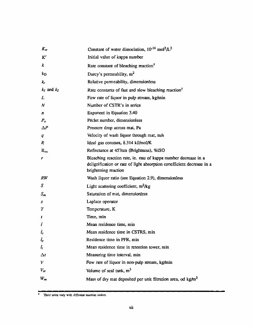
Constant of water dissociation, 10-14 mo12/L2
K'^Initial value of kappa number
Rate constant of bleaching reaction/.
kE•^Darcy's permeability, m2kr^ Relative permeability, dimensionlesski and k2^Rate constants of fast and slow bleaching reactionf
Fow rate of liquor in pulp stream, kg/minNumber of CSTR's in seriesExponent in Equation 3.40
Pe^ Peelet number, dimensionlessAP^Pressure drop across mat, Pa
Velocity of wash liquor through mat, m/sIdeal gas constant, 8.314 kJ/mol/K
Itoo^Reflectance at 457nm (Brightness), %ISOBleaching reaction rate, ie. rate of kappa number decrease in adelignification or rate of light absorption conefficient decrease in abrightening reaction
RW^Wash liquor ratio (see Equation 2.9), dimensionless
Light scattering coefficient, m2/kgS,,,^Saturation of mat, dimensionless
Laplace operatorTemperature, KTime, minMean residence time, minMean residence time in CSTRS, minResidence time in PFR, minMean residence time in retention tower, min
At^Measuring time interval, minV^ Fow rate of liquor in non-pulp stream, kg,/min
Volume of seal tank, m3W„,^Mass of dry mat deposited per unit filtration area, od kg/m2
Their units vary with different reaction orders.
xii
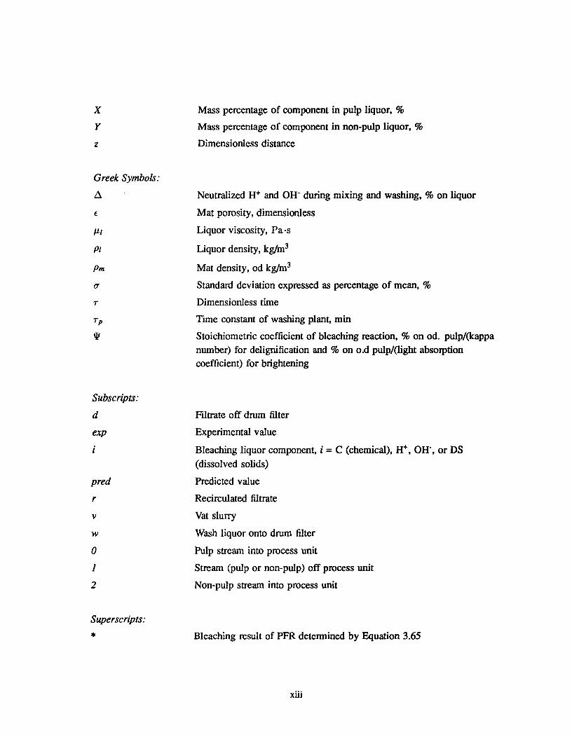
X^
Mass percentage of component in pulp liquor, %Mass percentage of component in non-pulp liquor, %Dimensionless distance
Greek Symbols:
A^Neutralized II+ and OH- during mixing and washing, % on liquorE^Mat porosity, dimensionless
Liquor viscosity, Pa •s
Liquor density, kg/m3
Pm^Mat density, od kg/m3o^ Standard deviation expressed as percentage of mean, %
Dimensionless timeTp^ Time constant of washing plant, min
Stoichiometric coefficient of bleaching reaction, % on od. pulp/(kappanumber) for delignification and % on o.d pulp/(light absorptioncoefficient) for brightening
Subscripts:
Filtrate off drum filter
exp^Experimental value
Bleaching liquor component, i = C (chemical), 1-1+, OH-, or DS(dissolved solids)
pred^Predicted valueRecirculated filtrate
Vat slurryWash liquor onto drum filter
0^ Pulp stream into process unit
1^ Stream (pulp or non-pulp) off process unit2^ Non-pulp stream into process unit
Superscripts:
Bleaching result of PFR determined by Equation 3.65

Abbreviations:CSTR^Continuous stirred tank reactorCSTRS^Continuous stirred tank reactors in series
DS^Dissolved solidsPFR^Plug flow reactorRTD^Residence time distributionTAC^Total available C12, % on pulp
Abbreviations for Bleaching Stage:C/D^Chlorination with C12 and 002 substitution (10 - 70% as active chlorine)
(C.+Dioo-x)^Simultaneous addition of x% (as active chlorine) C12 and (100-x)% (asactive chlorine) 002
CD^Chlorination with C12 and small percentage of 002 (5. 10% as activechlorine)
DI^First 002 bleaching stage
D2^ Second C102 bleaching stage
Dc^Chlorination with 002 and small percentage of C12 ( <50%)
(DxCloo-x)^Chlorination with sequential addition of x% (as active chlorine) C102followed by (100-x)% (312. Time delay between additions is not specified.
Ei^First alkaline extraction stage
Eo^First alkaline extraction with addition of 02
E2^ Second alkaline extraction stage
0^Oxygen delignification
x iv

ACKNOWLEDGMENTS
I extend my sincerest appreciation and thanks to my thesis supervisors, Dr. Patrick Tessier
and Dr. Chad Bennington for their guidance, kind support, encouragement and valuable discussions
throughout the course of this research, without which this work would not have been possible.
I am also indebted to Dr. Bruce Bowen and Dr. Richard Branion for providing valuable advice
and suggestions.
I wish to thank Patti Turner of PAPRICAN for providing information for the simulation of
brown stock washers.
I would appreciate academic assistance of Dr. Yu Qian, Dr. Ruhe Zhao, Mr. Ky Vu and Mr.
Scott Morgan.
I would like to thank my colleagues and also my friends, Mr. Xingsheng Qian and Mr. Lijun
Wang for sharing a pleasant time with them.
The consistent computer network support from Mr. Rick Morrison and Mr. Kristinn Kristinsson
is greatly acknowledged.
I would like to express my special thanks to Ms. Rita Penco for her patient assistance in my
literature search.
I am thankful to the other members of the PAPRICAN group at UBC and the staff of the chemical
engineering department office for their assistance.
I would like to thank the National Sciences and Engineering Research Council of Canada for
providing financial support and excellent computer facilities.
I am grateful to my little daughter, my husband and my parents in law for their contributions to
a happy family which is the most important for the success of my thesis.
Finally, my greatest thanks go to my parents for their love and enormous sacrifices for their
daughter.
XV
DEDICATION
x vi
CHAPTER I: GENERAL INTRODUCTION
CHAPTER 1
GENERAL INTRODUCTION
Pulp and paper mills are made up of a wide variety of process units which transform wood
into pulp and paper products. Numerous flows of pulp, water, chemicals and dissolved solids must
be recycled, leading to a high degree of interaction among the process units. Complicated physical
and chemical phenomena take place in the many unit operations. The kraft pulp process outlined in
Figure 1.1 is considered to be typical. There are three important process operations in converting
wood chips into bleached pulp: digestion, brown stock washing and bleaching. During digestion
with chemicals and heat, the lignin and other alkali-soluble constituents of wood are dissolved in
the cooking liquor and the fibres are liberated. The mixture of pulp and spent cooking liquor after
digestion, referred to as brown stock, is fed to a series of washers, where the spent cooking liquor is
separated from the pulp using fresh or reused water. The spent cooking liquor, also called weak black
liquor, is then delivered to the recovery system to recycle cooking chemicals and recover thermal
energy. The washed pulp is transferred to the bleach plant where the pulp is subject to a sequence
of chemical treatments to increase pulp brightness.
Industrial processes can be modeled mathematically based on mass, energy and momentum
balances. Computer simulation can be of considerable help in solving design and operation problems.
This is why there has been a tremendous increase in the use of computer simulation in the pulp
and paper industry (Roche and Bouchard, 1982; McConnell et al., 1992). The most common
applications have involved steady-state simulation, especially in areas of the process design and
operation optimization. Many commercial steady-state simulators have been available for pulp and
paper processes, such as GEMS (Edwards et al., 1983), MASSBAL (1983), PAPMOD (1988),
FlowCale (1983) and MAPPS (1984). For use in process control design, a few simulators, such
as GEMS, PAPDYN (1990) and MAPPS, have been modified by including the dynamics of storage
tanks to provide time-dependent simulation. These simulators, basically consisting of steady-state unit
models described by relatively simple algebraic equations, are inadequate to accurately characterize
the dynamic behavior of various pulp and paper processes. In order to help the pulp and paper industry
1
Make-upChemicals
'41111-Recovered
i
Chemicals
WashWater
Un
4^
Brown StockWashing
,leachedPulp
Recovery lo EnergyBlack Liquor
Bleaching Bleaching Chemicals-41-- Heat
Digestion
BrownStock
Cooking Liquor
Chapter 1: GENERAL INTRODUCTION
Wood Chips
Bleached Pulpto Market or
to Paper Machine
Figure 1.1: Kraft pulp process schematic.
increase process control abilities and understand the effect of dynamics on its operation, there is a
need for a more realistic dynamic simulator which provides detailed dynamic models of the process
units. Such a simulator can be used as a mathematical "pilot-plant" to investigate process behavior
of an actual plant and to test different control strategies. Interactions among the process units would
become evident and transient responses of the overall system to disturbances (such as changing feed
rates, failure of equipment or different operating strategies) could be predicted. Dynamic simulators
can also help new operators learn about the effects of operation changes and the benefits of properly
tuned control systems.
Powerful computer technologies are necessary to develop a new dynamic process simulator
for the pulp and paper industry. From a software point of view, there are several alternatives
2
CHAPTER I: GENERAL INTRODUCTION
for our purpose: from general languages to equation-oriented simulators. FORTRAN and C may
be employed but are unwieldy for complex applications. A good simulation package must be
robust, well-structured, versatile and user-friendly. We think that SIMNON, an equation-oriented
dynamic simulator, is a suitable choice. SIMNON was developed in the Department of Automatic
Control of the Lund Institute of Technology in 1979 (SIMNON, 1991). It is designed for simulating
dynamic systems whose behavior is represented by nonlinear, ordinary, differential or difference
equations. A complex system may be described as an interconnection of simpler subsystems. This
modular feature provides considerable flexibility for constructing plant models where unit models
can be easily modified and rearranged for different flowsheets. Advanced integration algorithms
are supplied to improve executive time and simulation accuracy for the long term as well as very
fast response. External modules written in FORTRAN or C may be embodied into the SIMNON
framework to enhance the capabilities in computation and system description. SIMNON has been
used for education and research in such diverse disciplines as automatic control, biology, chemical
engineering, economics and electrical engineering at many universities. The original version was
implemented in PC/DOS computers and a new version can be also run under the UNIX operating
system on Sun/Sparc workstations.
Using SIMNON as a platform, dynamic simulators for brown stock washers and a multistage
bleach plant have been developed. Firstly, we used the brown stock washers as an example to test
the applicability of SIMNON . The model developed for the brown stock washer can also be used for
describing the pulp washer in the bleach plant. A series of brown stock washers form a countercurrent
system of pulp and wash liquor with significant recycle existing within each stage. We will show
how the washer model incorporated into SIMNON can be used to study the dynamic behavior of a
multistage countercurrent washing system, including interactions among the washing stages and the
dynamic response of the washing plant to manipulation of the wash water flow rate and to major
process disturbances. We will also test and compare different control strategies for the washing plant
dueugh the use of the simulator.
Once satisfied that SIMNON was able to handle a relatively simple but very representative
process, our work moved on to a more difficult problem: a multistage bleach plant. Operations in the
3
Chapter I: GENERAL INTRODUCTION
bleach plant are very complicated mainly due to multistage chemical reactions with long retention
times, complex compositions of process streams and the large number of recycled flows. Few attempts
have been made to model pulp bleaching processes, particularly the dynamic behavior of the process.
To describe the dynamics of such a system, detailed investigations of the kinetics of the bleaching
reactions and the pulp flow in bleaching towers were made. A combination of SIMNON and a
FORTRAN algorithm was used to solve the partial differential equations which represent the reactor
behavior varying with position as well as time. The unit operation models and appropriate bleaching
kinetics were combined together to describe each bleaching stages. The integrated model can be used
to study transient responses in the final kappa number, brightness and residual chemicals to changes
in various process variables. A simulation model of a five stage bleach plant having a CDEDED
sequence was built up by connecting the corresponding stage models. The dynamic response of
different stages of the bleach plant were obtained when changes were made to the unbleached pulp
kappa number, production rate and chemical charge.
4

CHAPTER 2: MODELLING, SIMULATION AND COIVTROL OF BROWN STOCK WASHERS
CHAPTER 2
MODELLING, SIMULATION AND CONTROL OF BROWN STOCK WASHERS
2.1 Introduction
The primary purpose of the brown stock washing plant in a kraft pulp mill is to economically
remove the maximum amount of dissolved organic and soluble inorganic materials present in the pulp
at the end of the cooking or digestion of wood chips with the minimum amount of fresh or reused
process water. Therefore it has two effects on the pulping process. Firstly, it cleans the pulp for
bleaching treatments. Secondly, it is the first step in the recovery process which recycles the inorganic
products and recovers the thermal energy of organic components extracted from the wood. Better
washing leads to more pulping chemical recovery, less energy cost for the recovery evaporation,
reduced bleach chemical demand and decreased mill discharges of BOD, COD and AOX.
The washing plant possesses typical features of a pulp and paper process. It is a multiple input,
multiple output system with recycle loops and countercurrent flows. Each stream contains water,
fibres and dissolved solids. Therefore, this plant is a very good example to examine the capability
of SIMNON for developing a dynamic simulation of other pulp and paper processes. The model
developed for the brown stock washer is also useful in simulating washers in the bleach plant.
Dynamic simulation of brown stock washers has been done in previous studies (Perry et al., 1975;
Lundquist, 1980; Nase and Sjoberg, 1989; Turner et al., 1990), making it possible to compare our
results with theirs.
In this chapter, the dynamic mathematical model of a vacuum drum washer is described. Then
applications of the dynamic washer simulator are demonstrated through open-loop and closed-loop
simulations. The open-loop simulation was used to investigate the dynamic responses of a three-stage
brown stock washing plant to changes in wash liquor flow and process disturbances. The closed-loop
simulation was used to compare different control strategies.
5

Chapter 2: MODFI LING, SIMULATION AND CONTROL OF BROWN STOCK WASHERS
2.2 Process Description
Brown stock washing is carried out in a series of washers that form a countercurrent system. Each
washer represents a washing stage. The vacuum drum washer is the most commonly-used washer
in brown stock washing and also in bleach plants (Crotogino et al., 1987). Figure 2.2 shows a flow
diagram of a typical brown stock washing plant using three vacuum drum washers. The incoming
pulp stream (brown stock) is fed into the first stage and the wash water is added countercurrently.
The outgoing pulp stream from each stage goes to the next stage for further washing and the outgoing
filtrate is recirculated as dilution liquor for the incoming pulp or is used as the wash liquor for the
previous stage. The filtrate from the first stage is sent to the evaporator train. The washed pulp from
the last stage goes to the bleach plant.
Figure 2.2: Flow diagram of a three-stage vacuum drum washing plant.
The operation of a vacuum drum washing stage consists of several steps. Pulp enters the washer
at medium consistency (6-12%) and is diluted by recirculated filtrate to low consistency (0.75-2.5%)
before entering a vat which contains a wire-cloth covered drum. As the drum rotates through the vat
slurry, a lower pressure inside the drum extracts the liquid from the vat slurry with pulp forming a
mat on the surface of the drum. After the mat emerges from the slurry, liquid is further extracted
as it moves into the displacement washing zone where cleaner wash liquor is applied to displace
the dirty vat liquor. The mat is further dewatered and finally removed from the wire surface at a
6
CHAPTER 2: MODELLING, SIMULATION AND CONTROL OF BROWN STOCK WASHERS
medium consistency. The filtrate collected from the drum goes down through a drop leg to a seal
tank for deaeration and then is recirculated as dilution liquor or used as shower liquor on the previous
stage. The recirculated liquor flow rate is roughly ten times larger than the flow rate of the wash
liquor to the previous stage.
2.3 Model Development
2.3.1 Introduction
The great dependence of the other parts of the mill on the brown stock washing plant explains
the interest that has always been shown in it. Many projects have been carried out modelling washing
process, particularly the works of Norden et al. (1966; 1987), Tomiak (1974) and Cullinan (1986).
All these studies deal with the static operation of process, particularly for the purpose of designing the
washing plants and choosing their operating conditions. To improve the control of these processes, it
is necessary to know the connections between the action variables and the output variables in the form
of dynamic models. Some such studies have been carried out especially by Perry et al. (1975), Perron
and Lebeau (1977), Han (1989) and Turner et al. (1990). They all employed complicated mechanistic
models, involving fundamental fluid flow and mass transfer principles. A model integrating the
Norden efficiency factor with the dynamic tank seems to be best for describing mill washing systems
(Lundquist, 1980; Nase and Sjoberg, 1989). The present study dims at identifying a methodology
which can facilitate the simulation of washing plants and the evaluation of control strategies. The
analysis and modelling of a vacuum drum washing system are presented in this section.
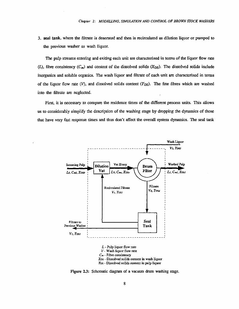
2.3.2 Process Variables and Analysis
A vacuum drum washing stage can be divided into the following three process units shown in
Figure 2.3:
1. dilution vat, where the incoming pulp at medium consistency is diluted to low consistency by
the recirculated filtrate,
2. drum filter, where a portion of the dissolved solids are separated from the fibres by thickening
and washing with cleaner wash liquor and
7
Wash Liquor
V2, YDS2
Washed Pulp
Li, Cntl , XDSI
Filtrate toPrevious Washer
4^VI, YDS/
,
Chapter 2: MODELLING, SIMULATION AND CONTROL OF BROWN STOCK WASHERS
3. seal tank, where the filtrate is deaerated and then is recirculated as dilution liquor or pumped to
the previous washer as wash liquor.
The pulp streams entering and exiting each unit are characterized in terms of the liquor flow rate
(L), fibre consistency (C.) and content of the dissolved solids (XDs). The dissolved solids include
inorganics and soluble organics. The wash liquor and filtrate of each unit are characterized in terms
of the liquor flow rate (V), and dissolved solids content (YDS). The fine fibres which are washed
into the filtrate are neglected.
First, it is necessary to compare the residence times of the different process units. This allows
us to considerably simplify the description of the washing stage by dropping the dynamics of those
that have very fast response times and thus don't affect the overall system dynamics. The seal tank
L - Pulp liquor flow rateV - Wash liquor flow rate
C. - Fibre consistencyXDS - Dissolved solids content in wash liquorYDS - Dissolved solids content in pulp liquor
Figure 23: Schematic diagram of a vacuum drum washing stage.
8

CHAPTER 2: MODELLING, SIMULATION AND CONTROL OF BROWN STOCK WASHERS
has a much longer residence time than the dilution vat and drum filter because of its large liquor
inventory. The filtrate stays in the seal tank for about 10 minutes. Pulp remains in the vat for
only a few seconds and passes over the drum in less than 1 minute. Therefore when modelling the
dynamics of a complete washing stage, it is assumed that the dilution vat and drum filter are operated
in quasi-steady state, i.e., their responses to changes in operating conditions are instantaneous. The
transient behavior of the seal tank governs the overall stage dynamics and is considered alone. The
models of the washing units, stage and entire plant are described below.
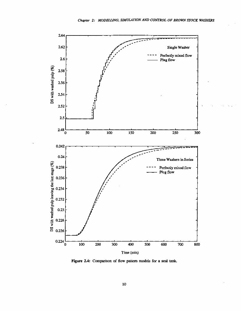
2.3.3 Modeling of Seal Tank
To describe the dynamics of the seal tank, plug flow and perfectly mixed flow models were
tested. The real seal tank should act somewhere between these two ideal limits. However, the effect
of different flow patterns in the seal tank on the dynamic behavior of the entire washing system is
diminished by strong interactions between the adjacent process units. Step responses of washed pulp
predicted using the two ideal flow models are approximately the same whether for a single washer
or a three-stage washing plant as shown in Figure 2.4. The perfectly mixed flow model was chosen
to represent the seal tank. This model consists of the following equations:
Overall mass balance:
dffst^(rd—li-14)dt^Vst • PI
and dissolved solid mass balance:
Carp^Vd • (YDSd YDS1)irscHst.p,
where 1131 is the percentage of liquor level in the total seal tank level, Vit is the seal tank volume.
The liquor density, pi, is a function of the temperature and dissolved solids concentration of the
liquor. Some empirical correlations for black liquor density have been reported (Venkatesh, 1985;
Terry, 1988; Branch, 1991). However, it is reasonable to assume a constant liquor density since the
dissolved solid content of the filtrate in brown stock washing is fairly small (<20 %).
(2.1)
(2.2)
9
2.64
2.62
2.6
238a.aa.I? 2.564*•S- -* 2.543
rnA
--
I
00
I0
0I
Single Washer
- - - - Perfectly mixed flowPlug flow
rI
t
I
t
-- --
Three Washers in Series
- — Perfectly mixed flowPlug flow
Chapter 2: MODELLING, SIMULATION AND COIVTROL OF BROWN STOCK WASHERS
-
I
I2.52
25
2'480 50^100^150^200^250^300
0.242
0.24
ts---2.°0.238
oo0....
rj 0.236
41 0.234
000.232
rz0al.
..g 0.2343.5 0.228-3"
E 0.226
0.224 ^0 100
^200^
300^400^500^600^700^800
Time (min)
Figure 2.4: Comparison of flow pattern models for a seal tank.
10
CHAPTER 2: MODELLING, SIMULATION AND COIVTROL OF BROWN STOCK WASHERS
Wash Liquor
Vat Slurry
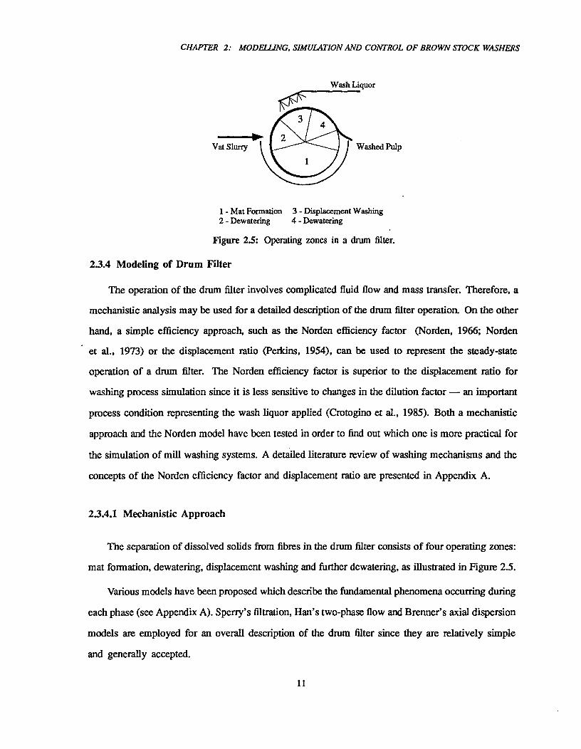
1 - Mat Formation 3- Displacement Washing2- Dewatering^4- Dewatering
Figure 2.5: Operating zones in a drum filter.
2.3.4 Modeling of Drum Filter
The operation of the drum filter involves complicated fluid flow and mass transfer. Therefore, a
mechanistic analysis may be used for a detailed description of the drum filter operation. On the other
hand, a simple efficiency approach, such as the Norden efficiency factor (Norden, 1966; Norden
et al., 1973) or the displacement ratio (Perkins, 1954), can be used to represent the steady-state
operation of a drum filter. The Norden efficiency factor is superior to the displacement ratio for
washing process simulation since it is less sensitive to changes in the dilution factor — an important
process condition representing the wash liquor applied (Crotogino et al., 1985). Both a mechanistic
approach and the Norden model have been tested in order to find out which one is more practical for
the simulation of mill washing systems. A detailed literature review of washing mechanisms and the
concepts of the Norden efficiency factor and displacement ratio are presented in Appendix A.
2.3.4.1 Mechanistic Approach
The separation of dissolved solids from fibres in the drum filter consists of four operating zones:
mat formation, dewatering, displacement washing and further dewatering, as illustrated in Figure 2.5.
Various models have been proposed which describe the fundamental phenomena occurring during
each phase (see Appendix A). Sperry's filtration, Han's two-phase flow and Brenner's axial dispersion
models are employed for an overall description of the drum filter since they are relatively simple
and generally accepted.
11

Chapter 2: MODFLUNG, SIMULATION AND COIVTROL OF BROWN STOCK WASHERS
Mat Formation As the drum rotates through the vat slurry, a lower pressure inside the drum
extracts the liquid from the vat slurry and a mat forms on the surface of the drum. This action is
described mainly based on Sperry's filtration equation (Sperry, 1916):
dG ^APdt = Wm
(2.3)
where:
G^= volume of the filtrate collected per unit filtration area, m
I^= residence time since the pulp slurry enters the filtration zone, s
AP = pressure drop across the mat, Pa
pi^= liquor viscosity, Pa.s
am^= specific resistance of the mat, in/kg
= mass of dry mat deposited per unit filtration area, od kg/m2
Both G and Wm can be expressed in term of the mat thickness, i.e.,
• HmG =
pm pi^ and Wm = pm • Hm^ (2.4)
‘-'171V • A
where:
H. = mat thickness, m
Cm, = vat consistency, %
PI^= liquor density, kg/m3
Pm = mat density, od kg/m3
When these expression for G and Wm are substituted into Equation 2.3 and the latter is integrated,
the mat thickness after filtration can be found for a given drum vacuum and vat consistency.
Dewatering and Displacement Washing After the mat emerges from the slurry, dewatering,
washing and further dewatering take place. The liquid flow through the mat during these steps is
12

CHAPTER 2: MODFI J ING, SIMULATION AND CONTROL OF BROWN STOCK WASHERS
represented by two-phase flow model proposed by Han (1989):
q dSdt,,,
•
c • Hm kr kr)
c • HIP
. pi(2.5)
where:
S.^= saturation of the mat, dimensionless
• = velocity of the wash liquor (zero for deWatering), m/s
1cD^= Darcy's permeability, m2
kr^= relative permeability, dimensionless
= mat porosity, dimensionless
Integration of Equation 2.5 yields the saturations at different positions in the drum rotary direction
(which is related to i). Then the profile of the mat consistency can be calculated from the saturation.
Displacement washing occurs when the wash liquor is applied to the mat. The dissolved solids
concentration profile in the mat during displacement washing and subsequent dewatering is described
using the axial dispersion model suggested by Brenner (1962):
Oc^1 02c Oc_Or P,Oz2 Oz
with initial and boundary conditions of
^c = 0^at r = 0 for all z
Oc = Pe • (c —1) at z = 0 for r > 0
8c
^
= 0^at z = 1 for r > 0OZ
where:
= (CDs, — CDsm )/(CDsv — Cpsw), dimensionless dissolved solids concentration
= Z1H„„ dimensionless distance
(2.6)
13
Chapter 2: MODELLING, SIMULATION AND CONTROL OF BROWN STOCK WASHERS
• = axial distance, m
Pe^= u • HmID, Peclet number, dimensionless
• = axial dispersion coefficient, m2/s
• = velocity of liquid through the mat, mis
• = t.^dimensionless residence time
CDSv • CDSm and CDSw = dissolved solids concentration in vat, mat and wash liquor respectively,
kg/m3
Brenner's model does not account for adsorption of dissolved solids on the fibre surface.
According to the observations of Poirier et al. (Poirier et al., 1987a), this simplification may not be
valid for the later stages of a washing plant, where the concentration of dissolved solids in the mat
liquor becomes much lower than that in the early stages. An additional term can be included in the
model to describe solute absorption (Sherman, 1964).
Equations 2.3 to 2.6 together constitute a mechanistic model for the drum filter operation. This
model describes the development of dissolved solids concentration and consistency across the drum
for a given consistency, dissolved solids concentration and flow rate of the vat slurry. The model
implies that there is no mixing of fluid along the drum rotary direction. Thus the outputs of the model,
such as dissolved solids concentration and consistency in the washed pulp, have a pure time delay in
response to input changes. This time delay, however, is negligible because of very short residence
time in the drum filter. The model also addresses the effects of drum speed and vacuum on the washing
results. Thus, this model could not only be used for designing the washing process control but also
for optimizing the washer operation. Unfortunately, this approach has limited application to the
mill washing operation since it requires complicated calculations and a great number of fundamental
parameters. The mat porosity, mat density, Peclet number and permeability are complicated functions
of process conditions as well as of fibre physical properties (compressibility, drainage, etc), which
are difficult to obtain from mill measurements.
14
CHAPTER 2: MODPTI.ING, SIMULATION AND CONTROL OF BROWN STOCK WASHERS
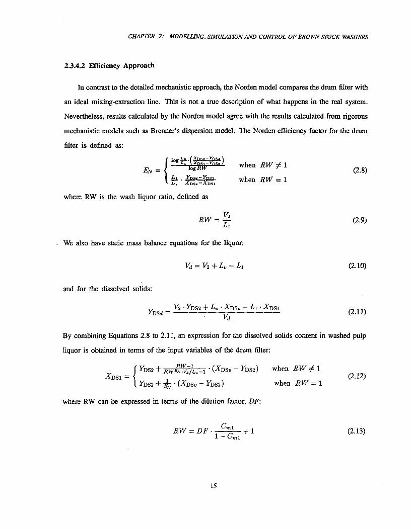
2.3.4.2 Efficiency Approach
In contrast to the detailed mechanistic approach, the Norden model compares the drum filter with
an ideal mixing-extraction line. This is not a true description of what happens in the real system.
Nevertheless, results calculated by the Norden model agree with the results calculated from rigorous
mechanistic models such as Brenner's dispersion model. The Norden efficiency factor for the drum
filter is defined as:
EN
= {log lit (xxDsv:Yyposs 2d)
log YtiA7^ypsd^sz ^L. A DStr^DS1
when RW 1
when RW = 1(2.8)
where RW is the wash liquor ratio, defined as
RW = —v2Li
. We also have static mass balance equations for the liquor:
Vd = V2 + Lv Ll
(2.9)
(2.10)
and for the dissolved solids:
YDSdV2 • YDS2 Lv • XDSv Ll • XDS1 (2.11)
Vd
By combining Equations 2.8 to 2.11, an expression for the dissolved solids content in washed pulp
liquor is obtained in terms of the input variables of the drum filter:
XDS1 =
RW —1 XDSv — YDS2)1 YDS2 + RwEN.Va/L„ —1 (
YDS2 + k • (xDst, — Ybs2)
when RW 1
when RW = 1(2.12)
where RW can be expressed in terms of the dilution factor, DF:
RW = DF Cmi 1
1 – Cmi(2.13)
15
XDSv — YDS2DR = XDSv — XDS1 (2.15)
Chapter 2: MODFI LING, SIMULATION AND COIVTROL OF BROWN STOCK WASHERS
As shown in Equation 2.12, the Norden method provides a straightforward relationship between
the dissolved solids content in washed pulp and the input variables of the drum filter. The value of the
Norden efficiency factor is available from mill data collected under conditions similar to the proposed
application. Therefore, this model is more practical for process simulation and control system design.
The outlet mat consistency, C„,/, is another input parameter of this model. A combination with the
simplified mechanistic model could be employed to account for the consistency as an independent
variable.
Since washing efficiency is often reported in tenns of displacement ratio in mills, it is useful
to relate the Norden efficiency factor to the displacement ratio in order to facilitate the application
of the Norden model to the process simulation. This relationship has been derived from the mass
balances around the drum filter and is shown by Equation 2.14:
EN= log RW
where DR is the displacement ratio and defined by Perkins (1954) as:
log^(RIVIDDRR)(2.14)
The ratio of the vat liquor flow rate to the filtrate flow rate leaving the filter, Lvilid, is approximately
equal to one because the recirculated filtrate constitutes the major part of both vat liquor and the
filtrate flow rate leaving the filter, roughly 90%. Therefore, Equation 2.14 can be simplified to be
io, RW—DR6 1—DR (2.16)= log RW
The Norden efficiency factor can be calculated by Equation 2.16 if the displacement ratio and the
corresponding wash liquor ratio are known.
2.3.5 Washing Stage and Plant Models
Table 2.1 summarizes the model equations used to simulate a single vacuum drum washing
stage. The drum filter is described based on Norden efficiency factor, the dilution vat as a static
perfect mixer and the seal tank as a dynamic perfectly mixed flow tank. This model retains the
16
L1 — LO1 — Cm° Cm1
{_ YDS2 + RwERNZ1L._i (XDSv — YDS2)
— YDS2 +^• (XDSt, — YDS2)XDS1 when RW 1
when RW = 1 (2.18)
3. Seal tank:^di ^(Vd — — Vr)^di ^Vat • Pi
dYD^Vd • (YDSd YDS1) di —^Vat • H at • pi
1. Dilution vat:= Lo + V,
LO • XDSO Vr • YDS1
2. Drum filter:
(2.17)
Vd = V2 A- —L1
(2.19)
Cm')^1 Cml
YDSd —^Vd
V2 • YDS2 Lv • XDSv — L1 XDS1
CHAPTER 2: MODELLING, SIMULATION AND COIVTROL OF BROWN STOCK WASHERS
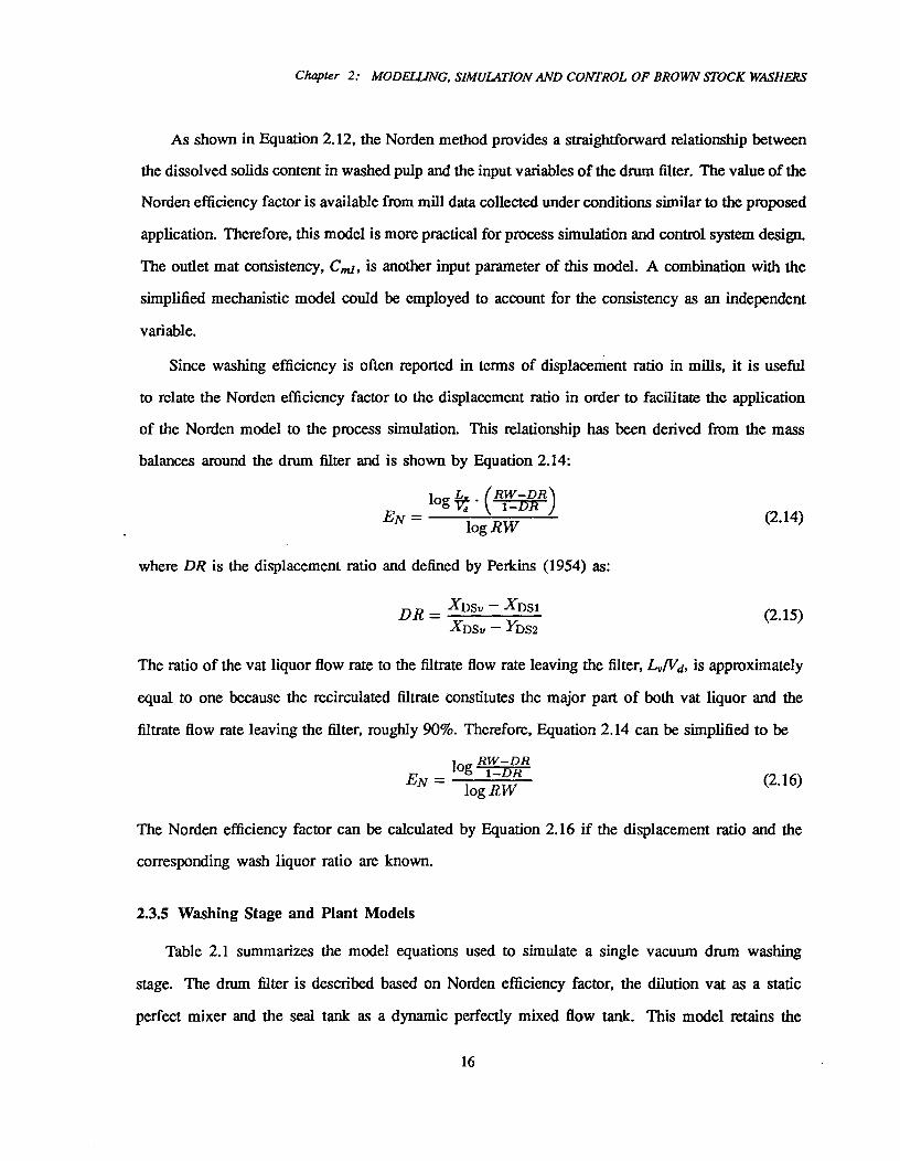
Table 2.1 Mathematical model of a washing stage.
dynamic characteristics of the washing system and the effects of major process conditions such as
dilution factor, production rate and incoming dissolved solids content. It has been written as a
computer module in SIMNON. The dynamic process model of a multistage washing plant can now
be constructed by connecting the separate washer modules. The structure of a simulation model
corresponding to the three-stage washing plant in Figure 22 is shown in Figure 2.6.
Black liquor.4-
Wash liquor
Washer Washer Washer1 2 3
1.=.4111.
Brown Stock Washed Pulp
Figure 2.6: Simulation model structure for a three-stage washing plant.
17
Chapter 2: MODMING, SIMULATION AND CONTROL OF BROWN STOCK WASHERS
2.4 Simulation of Process Dynamic Behavior
The countercurrent flows between pulp and wash liquor as well as the substantial recycles within
each unit lead to a complex dynamic behavior of the brown stock washing plant, which must be well
understood before a control system can be designed. The dynamic responses of a single washer and
a three-stage washing plant were investigated with the assistance of the washing process simulator
written in SIMNON. Input changes were made in the pulp production rate, dissolved solids content in
the pulp feed and wash liquor flow respectively. Changes in the pulp production rate and incoming
dissolved solids content can be due to variations in pulp digestion, blow tanks or pumps, while
the wash liquor flow is an important manipulated variable. The liquid levels in the seal tanks were
considered to be constant for any change so that the case studies could focus on the dynamic behavior
of the dissolved solids in the washed pulp and filtrate liquor. The initial steady-state conditions for
the simulation were obtained from operating data collected from an industrial washing plant with a
production rate of 400 odt/d (see Table 2.2).
2.4.2 A Single Washer
For a 15% step increase made in the pulp production rate, incoming dissolved solids content
or wash liquor flow rate, the responses of dissolved solids content in the washed pulp and in the
washer filtrate of a single washer are shown in Figure 2.7. The response in the filtrate is a slow,
first-order response. As a result of the very fast flow of the pulp stream, an instantaneous response
is observed in the washed pulp. It then become a slow first-order response because of the effect of
the recycle loop. The settling time (the time required for a step response to reach 95% of its new
steady-state value) is approximately 160 minutes for the change in dissolved solids in the pulp feed.
The settling time is about 70 minutes for both the change in wash liquor flow rate and the change in
production rate. The response magnitude is also similar for the change in the wash liquor flow and
for the change in the pulp production rate. The 15% change in these two variables produces about
12% steady-state change in the output dissolved solids content.
18

CHAPTER 2: MODFL LING, SIMULATION AND COIVTROL OF BROWN STOCK WASHERS
Table 2.2 Operating data of an industrial vacuum drum washing plant.
Variable Washer 1 Washer 2 Washer 3
Pulp onto washerConsistency (%) 6.90 8.50 12.8
Dissolved solids (%) 22.8 8.47 2.65
Vat slurryConsistency (%) 1.0 1.1 1.1
Dissolved solids (%) 19.4 6.73 1.53
Pulp off washerConsistency (%) 8.50 12.8 10.4
Dissolved solids (%) 8.47 2.65 0.537
Wash liquorDissolved solids (%) 6.71 1.50 0.0
Seal tankVolume (m3) 1067 861 683Level (%) 23.3 33.5 33.3
Dissolved solids (%) 18.9 630 1.43
Dilution factor 2.58 2.52 2.59
Wash liquor ratio 1.24 1.37 1.3
Displacement ratio 0.83 0.75 0.6
Norden efficiency factor 4.29 2.96 2.25
2.43 Three Washers in Series
Figures 2.8 to 2.10 show the responses of each washing stage in a three washer plant to a step
change in the pulp production rate, incoming dissolved solids content and wash liquor flow rate. It
took less than 1 second CPU time of a Sun/SPARC station 2 to simulate these dynamic responses
over a period 2000 minutes. The responses are much slower than those of the single washer due
to strong interactions between the stages. It took more than ten hours to reach the new level of
dissolved solids removal following the manipulation of the wash liquor flow rate. Such an unusually
slow response can often confuse the operator, who may never see the full results of his action during
19
9.4
9.2
8.8
8.6
8.4
8.2
Chapter 2: MODFILING, SIMULATION AND CONTROL OF BROWN STOCK WASHERS
_ (A)
100^
300^400^500^600
(B)
•
100^200^300^400^500^600
Time (min)
Figure 2.7: Dynamics of a single washer: step response in (A) dissolved solids in washedpulp and (B) dissolved solids in filtrate. A 15% increase is made at t=50 minutes in (a) pulp
production rate, (b) dissolved solids in pulp feed and (c) wash liquor applied on the last stage.
.5
22
213
21
20.5
20
19.5
19
18$
18
17$
17
20
CHAPTER 2: MODELLING, SIMULATION AND COIVTROL OF BROWN STOCK WASHERS
a shift An instantaneous response of washed pulp was observed when the pulp production rate or
wash liquor flow rate was changed, but not when the incoming dissolved solids content changed.
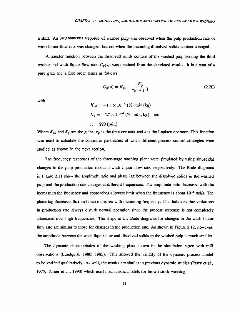
A transfer function between the dissolved solids content of the washed pulp leaving the third
washer and wash liquor flow rate, Gp(s), was obtained from the simulated results. It is a sum of a
pure gain and a first order terms as follows:
with
pGp(s) = Kpo +
Krp • s + 1 (2.20)
Kpo = —1.1 X 10⁻⁴ (% • min/kg)
Kp = -6.7 x 10⁻⁴ (% • min/kg) and
rp = 223 (min)
Where Kpo and Kp are the gains, rp is the time constant and s is the Laplace operator. This function
was used to calculate the controller parameters of when different process control strategies were
studied as shown in the next section.
The frequency responses of the three-stage washing plant were simulated by using sinusoidal
changes in the pulp production rate and wash liquor flow rate, respectively. The Bode diagrams
in Figure 2.11 show the amplitude ratio and phase lag between the dissolved solids in the washed
pulp and the production rate changes at different frequencies. The amplitude ratio decreases with the
increase in the frequency and approaches a lowest limit when the frequency is about 10-3 rad/s. The
phase lag decreases first and then increases with increasing frequency. This indicates that variations
in production rate always disturb normal operation since the process response is not completely
attenuated over high frequencies. The shape of the Bode diagrams for changes in the wash liquor
flow rate are similar to those for changes in the production rate. As shown in Figure 2.12, however,
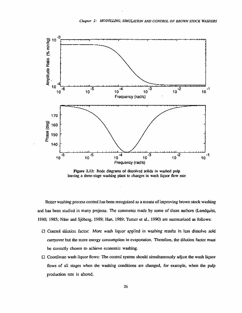
the amplitude between the wash liquor flow and dissolved solids in the washed pulp is much smaller.
The dynamic characteristics of the washing plant shown in the simulation agree with mill
observations (Lundquist, 1980; 1985). This allowed the validity of the dynamic process model
to be verified qualitatively. As well, the results are similar to previous dynamic studies (Perry et al.,
1975; Turner et al., 1990) which used mechanistic models for brown stock washing.
21
1400 1600400^600^800^1000 1200 1800 2000
Chapter 2: MODE]. LING, SIMULATION AND CONTROL OF BROWN STOCK WASHERS
13
12
11
10
(A)
200^400^600^800 1000 1200 1400 1600 1800 2000
Time (min)
Figure 2.8: Dynamics of 1st stage of a three stage washing plant: step response in (A) dissolved solids inwashed pulp and (B) dissolved solids in filtrate. A 15% increase is made at 150 minutes in (a) pulp
production rate, (b) dissolved solids in pulp feed and (c) wash liquor applied on the last stage.
22

CHAPTER 2: MODELLING, SIMULATION AND CONTROL OF BROWN STOCK WASHERS
5.5
(A)
4.5
-S 33
A 13
200^400^600^800 1000 1200 1400 1600 1800 2000
(B)
200^400^600^800^1000 1200 1400 1600 1800 2000
Time (min)
Figure 2.9: Dynamics of 2nd stage of the three stage washing plant: step response in (A) dissolved solids inwashed pulp and (B) dissolved solids in filtrate. A 15% increase is made at t=50 minutes in (a) pulp
production rate, (b) dissolved solids in pulp feed and (c) wash liquor applied on the last stage.
11
10
23
23
Chapter 2: MOD LUNG, SIMULATION AND COIVTROL OF BROWN STOCK WASHERS
1.4
g=^1.2
.gt.5; 0.8
A0.6
,..).2to 0.43.
002
(A)
0^200^400^600^800^1000 1200 1400 1600 1800 2000
33(B)
.,
'
200^400^600^800 1000 1200 1400 1600 1800 2000
Time (min)
Figure 2.10: Dynamics of 3rd stage of a three stage washing plant: step response in (A) dissolved solids inwashed pulp and (B) dissolved solids in filtrate. A 15% increase is made at 160 minutes in (a) pulp
production rate, (b) dissolved solids in pulp feed and (c) wash liquor applied on the last stage.
030
24
N-1,11-9"
10 -5
10 :
0 -2c"-T5 1 0 -cca)-a
E< 10^•
10 -6 10
-410
-3
Frequency (rad/s)
.^. .
-2^1-10^10
-1 0
-40
-50
CHAPTER 2: MODMING, SIMULATION AND CONTROL OF BROWN STOCK WASHERS
10 -6^
10 -5^
10 -4^
10 -3^10 -2
Frequency (rad/s)
Figure 2.11: Bode diagrams of dissolved solids in washed pulpleaving a three-stage washing plant to changes in pulp production rate
2.5 Control Strategy Evaluation
2.5.1 Washing Process Control
Attention to brown stock washing has been growing for the following reasons:
O Reduced dissolved solids carry over to bleach plant is suggested as a way to help meet
more strict environmental regulations on bleaching effluents.
O Increasing energy prices have made it very desirable to reduce the amount of water to be
evaporated.
O The importance of good washing for product quality is better understood.
25
Chapter 2: MODE! . TING, SIMULATION AND CONTROL OF BROWN STOCK WASHERS
..,e133 10-3
^• 1^•I^V^ I
.?
Ee....cocra)Ve=.r).E -< .110 -476—^. . ..
-510^10
'10 -4^10
-3^10 -2
Frequency (rad/s)
170-a(2) 160-0wPrs 150.c0_
140
10 -6^
10 -5^
10 -4^
10 -3^
10 -2
Frequency (rad/s)
Figure 2.12: Bode diagrams of dissolved solids in washed pulpleaving a three-stage washing plant to changes in wash liquor flow rate
Better washing process control has been recognized as a means of improving brown stock washing
and has been studied in many projects. The comments made by some of these authors (Lundquist,
1980; 1985; /lase and Sjoberg, 1989; Han, 1989; Turner et al., 1990) are summarized as follows:
El Control dilution factor: More wash liquor applied in washing results in less dissolve sold
carryover but the more energy consumption in evaporation. Therefore, the dilution factor must
be correctly chosen to achieve economic washing
El Coordinate wash liquor flows: The control system should simultaneously adjust the wash liquor
flows of all stages when the washing conditions are changed, for example, when the pulp
production rate is altered.
26
CHAPTER 2: MODFI LING, SIMULATION AND CONTROL OF BROWN STOCK WASHERS
O Coordinate liquid levels of seal tanks: Control of the seal tank levels and control of the dissolved
solids removal are all based on manipulation of the countercurrent wash liquor flows. A proper
control strategies for the seal tank levels is important to eliminate interactions between the tank
levels and interactions between the tank levels and dissolved solids removal.
O Control dissolved solids removal: The washing control system should have ability to reduce
the process variability to maintain optimum dissolved solids removal.
O Detect disturbances: Sensors to monitor disturbances are desired to decide the appropriate
operating conditions when the washing system is disturbed.
O Inform the operator about disturbances and efficiencies: This can give an early warning when
a bad situation is developing. It can also provide a good basis for continuous tuning and more
long-term improvements of the process.
The dilution factor proposed by Korhonen (1979) has been widely accepted as a main control
variable. Turner et al. (1991) designed a cascade feedforward control system which was able to
eliminate oscillations of seal tank levels. However the vast majority of washing plants are still
operated without any significant control systems, where operator involvement is the major control
element. Automatic control of drum washers is limited primarily to level control loops (Tumer et
al., 1990). The drum rotation speeds are adjusted to maintain the dilution vat levels constant and the
flow rates of wash liquor are manipulated to maintain liquid levels constant in the seal tanks.
In this work, the process dynamic simulator was used to study how washing plant control might
be further improved. In particular, three control strategies for a three-stage vacuum drum washing
plant are compared and evaluated. The process dynamic behavior of the washing plant was discussed
in the previous section.
Strategy 1 only controls the liquid levels in the seal tanks with no action to correct dissolved
solids removal. The control loops for the seal tank levels are shown as dot-dashed lines in Figure
2.13. Proportional controllers were used for the seal tank level.
Strategy 2 not only controls the seal tank levels but also the dissolved solids removal by means of
feedback control. The feedback control system measures the dissolved solids content of washed pulp
27

Chapter 2: MODE!. LING, SIMULATION AND CONTROL OF BROWN STOCK WASHERS
leaving the last washer and adjusts the wash liquor flow rate onto that washer to maintain the desired
dissolved solids content in the washed pulp. It also simultaneously adjusts all upstream wash liquor
flow rates by the same amount (dotted lines in Figure 2.13). The feedback controller for dissolved
solids removal was a PI controller. The controller parameters were found by using Dahlin's tuning
rule. This rule results in a first-order closed-loop response and requires only one tuning parameter.
Strategy 3 expands Strategy 2 by adding a feedforward control for dissolved solids removal. The
feedforward control monitors the production rate as a function of the consistency and flow rate of the
brown stock onto the first washer, and maintains the dilution factor by adjusting wash liquor flow rates
in the washing system. The feedforward control is illustrated by dashed lines in Figure 2.13. The
feedback control shown by the dotted line was used to determine the set point of the dilution factor.
All these control strategies are based on existing on-line instrumentation for brown stock washing.
Measurement of the liquid level in the seal tank is required for all the strategies. In addition,
measurement of the dissolved solids concentration in washed pulp is required for Strategy 2 and
Strategy 3. There is also a need for Strategy 3 to measure the incoming slurry flow rate and
consistency. Measuring the tank level and slurry flow rate are already successful technology. There
are different types of on-line consistency indicators on the market, such as blade type transmitters
and microwave gauges (Woodard, 1988), etc. The dissolved solids carryover can be measured based
on mat liquor conductivity (Wigsten, 1988). An optical sensor to monitor the dissolved solids
concentration has recently been developed (Edlund et al., 1992).
2.5.2 Results and Discussion
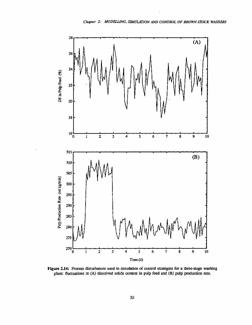
In order to give the control strategy simulation a realistic result, time series of the pulp production
rate and the dissolved solids content in pulp feeds over a period of 10 days which we derived from a
mill data were used as the process disturbances of the simulation. The power spectrum corresponding
to the mill data showed eight peaks. We, therefore, selected the eight corresponding frequencies and
amplitudes to represent the incoming dissolve solids variations as shown in Figure 2.14. Also shown
in this figure are the production rate variation composed of a square wave with a period of two
days and appropriate random noise. Figure 2.15 shows the dissolved solids carryover (kg dissolved
28

Tank Level Controller0 Analyzer Transmitter 0 Dissolved Solids Controller
I Frcedforward Control
T'41+
Redbrick Control
Brown Stock
Black Liquor
Seal Tank2
•Washed Pulp
Seal Tank1
Seal Tank3
CHAPTER 2: MODE! LING, SIMULATION AND COIVTROL OF BROWN STOCK WASHERS
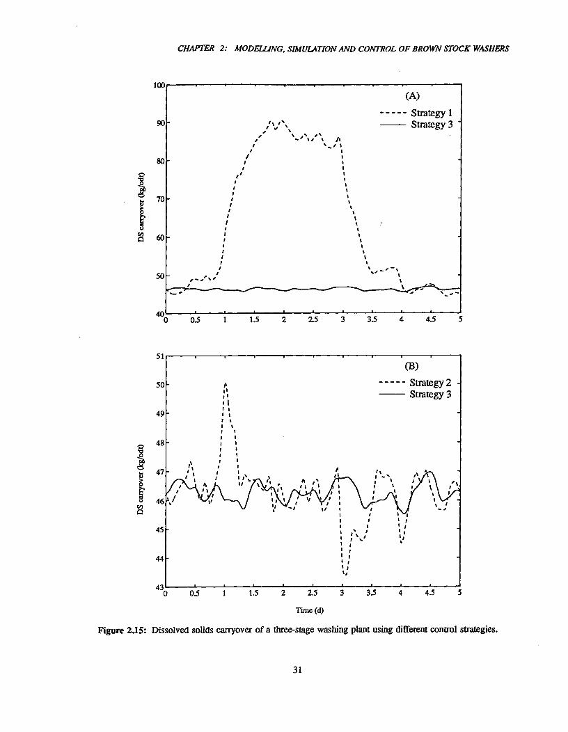
Figure 2.13: Control layout of a three-stage vacuum drum washing plant.
solids/odt pulp) obtained by the different control strategies in response to the process disturbances for
the first five days. The CPU time for each response simulation was about 10 seconds. Large increase
in the dissolved solids carryover resulted from the disturbances when the system was controlled using
Strategy 1 (see dotted line in Figure 2.15A). In contrast, the dissolved solids carryover of Strategy 3
was relatively constant (see solid line in Figures 2.15A). Strategy 2 yielded a slower compensation
for production rate disturbances than Strategy 3 (see Figure 2.15B). It took up to ten hours to pull
the dissolved solids content in the washed pulp back to the set point. Table 2.3 lists the means and
variances of dissolved solids carryover during the 10 days resulting from the three control strategies. It
is apparent that both Strategy 2 and Strategy 3 can give much smaller means and variance of dissolved
solids carryover than Strategy 1. This improvement has economic and environmental significance,
not only for the washing plant but also for the other departments in the mill.
Variations in the seal tank levels of Strategy 3 are larger than those of the other two control
strategies because it requires more vigorous manipulation of the wash liquor flow rate for rapid
29
22
18
16
315
310
1
\
\—
I\
I/I
\I
\\`k 1 /, It
1^2^3^4^5^6^7^8^9^10
1
\/
\,/i
I
\
Chapter 2: MODELLING, SIMULATION AND CONTROL OF BROWN STOCK WASHERS
28
26
ii
(B)
305gE:115 300
tc4
295
g 290..=8Z 285
2 280
275 A,,AMI
2700 1^2^3^4^5^6^7^8^9^10
Time (d)
Figure 2.14: Process disturbances used in simulation of control strategies for a three-stage washingplant: fluctuations in (A) dissolved solids content in pulp feed and (B) pulp production rate.
30
CHAPTER 2: MODELLING, SIMULATION AND COlVTROL OF BROWN STOCK WASHERS
80±2..........„-.8g1.,^70->o
i'rnA 60
50
1.5^
2
51
50
49
48
47
46
45
44
0.5^1^1.5^2^2.5^
3^
4
Time (d)
Figure 2.15: Dissolved solids carryover of a three-stage washing plant using different control strategies.
31
Chapter 2: MODELUNG, SIMULATION AND CONTROL OF BROWN STOCK WASHERS
Table 23 Mean and variance of dissolved solids carryover resulting from three control strategies.
Dissolved solidscarryover Strategy 1 Strategy 2 Strategy 3
Mean (kg/odt) 63.6 46.3 46.3Variance (% on mean) 27 2.6 0.68
Initial operating conditions listed in Table 22.Process distubances shown in Figure 2.14.
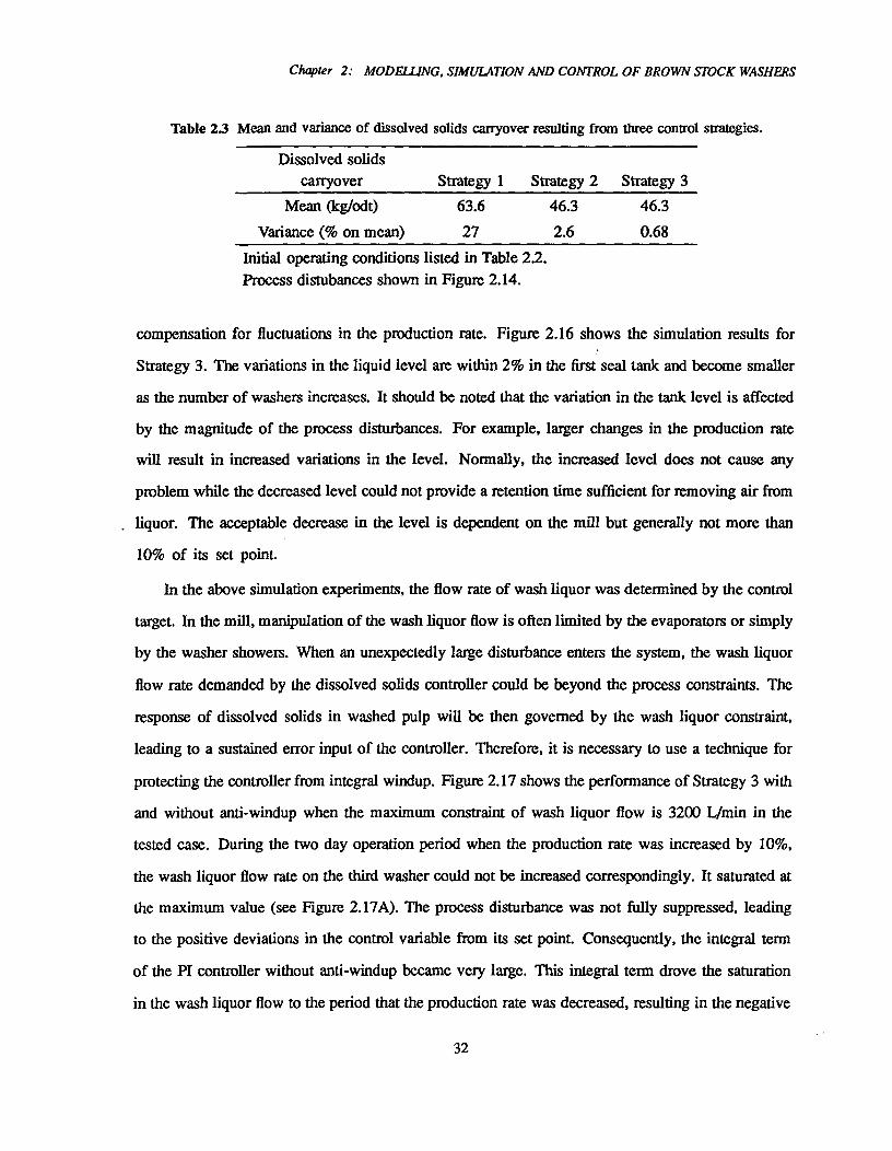
compensation for fluctuations in the production rate. Fig= 2.16 shows the simulation results for
Strategy 3. The variations in the liquid level are within 2% in the first seal tank and become smaller
as the number of washers increases. It should be noted that the variation in the tank level is affected
by the magnitude of the process disturbances. For example, larger changes in the production rate
will result in increased variations in the level. Normally, the increased level does not cause any
problem while the decreased level could not provide a retention time sufficient for removing air from
liquor. The acceptable decrease in the level is dependent on the mill but generally not more than
10% of its set point.
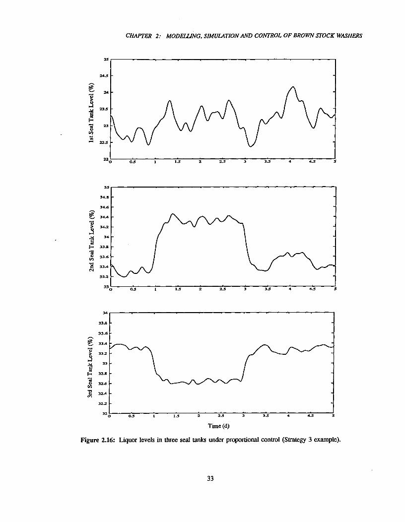
In the above simulation experiments, the flow rate of wash liquor was determined by the control
target. In the mill, manipulation of the wash liquor flow is often limited by the evaporators or simply
by the washer showers. When an unexpectedly large disturbance enters the system, the wash liquor
flow rate demanded by the dissolved solids controller could be beyond the process constraints. The
response of dissolved solids in washed pulp will be then governed by the wash liquor constraint,
leading to a sustained error input of the controller. Therefore, it is necessary to use a technique for
protecting the controller from integral windup. Figure 2.17 shows the performance of Strategy 3 with
and without anti-windup when the maximum constraint of wash liquor flow is 3200 L/min in the
tested case. During the two day operation period when the production rate was increased by 10%,
the wash liquor flow rate on the third washer could not be increased correspondingly. It saturated at
the maximum value (see Figure 2.17A). The process disturbance was not fully suppressed, leading
to the positive deviations in the control variable from its set point. Consequently, the integral term
of the PI controller without anti-windup became very large. This integral term drove the saturation
in the wash liquor flow to the period that the production rate was decreased, resulting in the negative
32
32 0 0.5 i 1.5 2 2.5 3 3.5 4 4.5 5
34
33.8
33.6,--,
63, 33.4
7..)> 33.2
41 33[-■ 32.8
1 32.6
15i...^32.4
VI
32.2
35
34.8
34.6
34.4
34.2
34
33.8
33.6
33.4
33.2
330 0.5
^1^
1.5^
2^
2.5^
3^
3.5^
4^
4.5^
5
CHAPTER 2: MODELLING, SIMULATION AND CONTROL OF BROWN STOCK WASHERS
Time (d)
Figure 2.16: Liquor levels in three seal tanks under proportional control (Strategy 3 example).
33

Chapter 2: MODF7 LING, SIMULATION AND CONTROL OF BROWN STOCK WASHERS
deviations in the process response (See Figure 2.17B). Since the controller with anti-windup can
give an integral modification when the saturation occurs, it can then follow rapidly the decrease in
production rate and take the correct control action.
2.6 Conclusions
This chapter is concerned with the modelling, simulation and control of a countercurrent brown
stock washing plant. The mathematical model based on the Norden efficiency factor and dynamic
seal tank appears to accurately represent the mill washer operation. This model can be used as a
simple but useful method for process simulation and control development.
The open-loop responses of three stage washing plants were simulated for changes in the pulp
production rate, incoming dissolved solids content and wash liquor flow rate. These examples showed
strong interactions and quick-slow mixing dynamics of the countercurrent washing system. It is
therefore very difficult to achieve good washing by manual control of a washing plant.
It was also showed how a good dynamic simulator could be used to develop and evaluate process
control strategies. Through use of typical process disturbances, three different control strategies
were compared. Automatic control of wash liquor flow applied in washing system can efficiently
compensate for the effect of process disturbances, resulting in uniform and reduced dissolved solids
carryover. The combination of feedforward and feedback control has much faster suppression on the
effect of variations in production rate than feedback control only.
SIMNON was well suited to the washing plant simulations, showing promise in the development
of dynamic simulators for other pulp and paper processes. Therefore, the use of SIMNON was
extended in the remainder of this study to a bleach plant.
2.7 Recommendations and Suggestions for Future Work
1. To test the sensitivity of the washer discharge consistency to changes in process conditions.
The present model assumes that the discharge consistency is constant when the wash liquor
flow or pulp production rate is changed.
34
CHAPTER 2: MODELLING, SIMULATION AND COIVTROL OF BROWN STOCK WASHERS
3250.....1
b 32004g
Vs.en 3150PA580CI';:.^3100-11
3300
3050
300°0
79
70
61,-,t-a5t,^52
k 43 -v)A
34
(A)— With Anti-Windup— Without Anti-Windup
I
1^2^3^4^5^6^7^8^9^10
(B)— With Anti-Windup— Without Anti-Windup -
•I
I^ I
%^ I%^ 1
%^ 1• •
I%^.^,-•^I s•‘^, ... •^S...,^..^ r% ,
0%,%^I^ ,.. %,...,^
1^I...,./
1^2^3^4^5^6^7^8^9^10
Time (d)
Figure 2.17: Effects of anti-windup on control performance.
35

Chapter 2: MODE! LING, SIMULATION AND CONTROL OF BROWN STOCK WASHERS
2. To develop a simplified mechanistic model or modify the Norden model to show the effects
of adsorption phenomena, drum speed, vacuum, vat consistency, etc. These factors are not
accounted for by the present model.
3. To apply the model to more problems. Examples include extending the present simulator
to other washing process flowsheets and washer configurations, optimizing wash liquor
application levels, and simulating washing control systems which may include secondary
loops (e.g., control of drum speed and recirculated liquor flow rate) in addition to the control
loops of wash liquor flow.
36
CHAPTER 3: MODELING AND SIMULATION OF A BLEACH PLANT
CHAPTER 3
MODELING AND SIMULATION OF A BLEACH PLANT
3.1 Introduction
Pulp bleaching is the chemical treatment of cellulosic fibre to increase pulp brightness by
removal or modification of the light-absorbing lignin left in the pulp while preserving pulp strength
characteristics. Bleaching can also increase pulp cleanliness to make pulp suitable for the manufacture
of printing and tissue grade paper.
The primary objectives in operating a bleaching plant are product brightness, production rate,
operation costs and environmental pollution. Today, environmental awareness is on the increase and
the kraft pulp industry is facing tougher regulations on bleach plant effluents. A dynamic bleaching
process simulator would be a very helpful tool for testing new bleaching operations and developing
process control to meet this challenge. Possible benefits from improved bleaching process control
include lower chemical demand and thus reduced pollution discharge while maintaining high pulp
quality. However, early attempts to formulate mathematical descriptions of bleach plant operations
have taken into account only the bleaching kinetics and the steady-state mass balances. No study has
touched on the bleach plant as a whole to reveal interactions within the system.
The dynamic process modelling presented in this chapter is based on fundamental flow phenom-
ena as well as chemical kinetics. The flow patterns of pulp slurries in bleaching towers were studied
and modeled by means of tracer responses. Based on the cluumophoric theory and experiments, a
correlation, which relates models of the delignification and brightening processes, was established.
Unit operation models for mixing, reaction and washing were formulated as mass balance equations.
It is a difficult problem to determine what type of bleaching sequence to simulate since bleaching
technology is rapidly changing in the 1990's due to environmental pressures. A CDEDED five
stage bleach plant, which is a conventional sequence for producing fully bleached haft pulps, was
chosen as an example in the present work. This choice is primarily due to the fact that there is suf-
ficient information on pulp bleaching kinetics, available in the literature, for modelling a CDEDED
37
Chapter 3: MODELING AND SIMULATION OF A BLEACH PLANT
sequence. Another reason is that such chlorine-based bleaching sequences with modifications are still
widely used in commercial bleached lcraft pulp manufacture. There are many chemical and physical
similarities among the various pulp bleaching sequences in current use. The present study can be
used as a basis for modelling other types of chlorine-based sequences and even bleaching processes
with novel chemicals. The process simulator written using SIMNON's modular approach can be
flexibly adapted to these new changes. Bleaching kinetic models from the literature were evaluated
and incorporated in the process simulator. Some of them were modified and expanded. An overall
model for the CDEDED plant is presented. The dynamic behavior of different stages in response to
changes in the chemical charge, incoming kappa number and production rate are illustrated.
3.2 Process Description
Bleaching is usually carried out in a continuous sequence made up of several stages with each
stage utilizing different chemicals and conditions. In the earlier stages of the bleaching sequence the
emphasis is on lignin removal while in the later stages the emphasis is placed on lignin decolourization
to develop brightness. Each stage is a combination of mixing, reaction and washing, and consequently,
different pieces of equipment are involved: 1) mixers to achieve a uniform mixture of fibres with
bleaching chemicals and steam, 2) a retention tower to provide time for chemical diffusion and
reaction and 3) a washer to separate the treated fibres from the soluble reacted material and spent
chemicals. Steam may be used in the stage to heat the pulp slurry to the reaction temperature.
Filtrate from each washer is recycled within the stage for dilution of the pulp slurry to the desired
inlet consistency and may be delivered to the previous stages for pulp washing
In the CDEDED bleaching sequence, the initial CDE sequence uses chlorine and chlorine dioxide
followed by extraction with sodium hydroxide to solubilize and remove the lignin in pulp. Chlorine
dioxide is applied at a low percentage in the order of 10% to the first chlorination stage to protect
pulp strength. The succeeding DED sequence employs chlorine dioxide and sodium hydroxide to
brighten the pulp. A flowsheet of a bleach plant with the CDEDED sequence is shown in Figure 3.18.
In the first CD stage, the unbleached pulp is often diluted to low consistency (s, 3.5%) and mixed
with 02 and 002. Then the bleaching reaction is completed in the CD tower and water-soluble
38
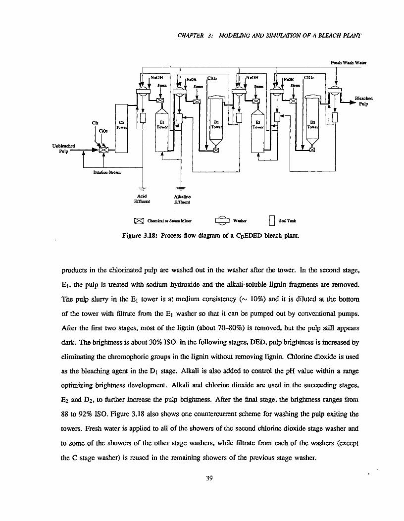
CHAPTER 3: MODELING AND SIMULATION OF A BLEACH PLANT
1:5-‹ Chanical or Steam Mixer^ED Washer^Seal Tank
Figure 3.18: Process flow diagram of a CDEDED bleach plant.
products in the chlorinated pulp are washed out in the washer after the tower. In the second stage,
Eli the pulp is treated with sodium hydroxide and the alkali-soluble lignin fragments are removed.
The pulp slurry in the El tower is at medium consistency (r- 10%) and it is diluted at the bottom
of the tower with filtrate from the El washer so that it can be pumped out by conventional pumps.
After the first two stages, most of the lignin (about 70-80%) is removed, but the pulp still appears
dark. The brightness is about 30% ISO. In the following stages, DED, pulp brightness is increased by
eliminating the chromophoric groups in the lignin without removing lignin. Chlorine dioxide is used
as the bleaching agent in the DI stage. Alkali is also added to control the pH value within a range
optimizing brightness development. Alkali and chlorine dioxide are used in the succeeding stages,
E2 and D2, to further increase the pulp brightness. After the final stage, the brightness ranges from
88 to 92% ISO. Figure 3.18 also shows one countercurrent scheme for washing the pulp exiting the
towers. Fresh water is applied to all of the showers of the second chlorine dioxide stage washer and
to some of the showers of the other stage washers, while filtrate from each of the washers (except
the C stage washer) is reused in the remaining showers of the previous stage washer.
39

Chapter 3: MODELING AND SIMULATION OF A BLEACH PLANT
In recent years, significant modifications in bleaching technology have taken place in order to
meet the increasingly stringent environmental regulations. Chlorine dioxide has been substituted
for most or all of chlorine in order to eliminate dioxin formation and decrease AOX generation.
Oxygen has been used to enhance the alkaline extraction to permit the removal of additional lignin.
Research is also underway to find economical and environmentally friendly chemicals for bleaching
pulp. Nevertheless, all typical bleaching operations are involved in the CDEDED sequence. Major
changes are usually associated with the use of different chemicals. Thus simulation of the CDEDED
sequence can serve as a starting point for modeling current and future bleaching technologies.
3.3 Model Development
33.1 Process Variables and Analysis
The mathematical model developed for a multistage bleach plant should have the ability to
address the interactions of important process variables within and between each bleaching stage.
Fundamental chemical and physical aspects should be identified by the process analysis to allow an
overall description of the bleach plant to be made. The process units and variables to be considered
for a single bleach stage are shown in Figure 3.19.
The pulp production rate of a bleaching plant is not constant due to variations in the flow rate and
consistency of the slurry entering the plant. Higher production rates need more chemicals to achieve
the desired product brightness. Increasing the production rate also decreases the slurry residence
time in the bleaching system. Variation in the kappa number of the pulp entering the bleaching
plant is an important disturbance. Fibre consistency, temperature and chemical charge of each stage
determine the bleaching reaction rate. The pH of the bleaching liquor is another vital factor for some
bleaching reactions. pH values could be changed due to mixing, washing and bleaching reactions.
The dissolved solids, especially organic dissolved substances, could react with bleaching agents if
they enter the bleaching process. Efficient washing is essential to decrease dissolved solids carryover
and thus to reduce chemical consumption. In a CEDED bleach plant, the kappa number after the El
40
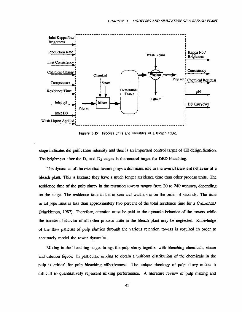
Production Rate
Inlet Consistency" ,
Chemical Charge
Temperature
Residence Time
Inlet pH
Inlet DS
Wash Liquor Applied
Kappa NodBrightness
Consistency
Chemical Residual
PH
DS Carryover
Inlet Kappa NodBrightness
Wash Liquor
ChemicalPulp out
Filtrate
Pulp in
RetentionTower
CHAPTER 3: MODELING AND SIMULATION OF A BLEACH PLANT
Figure 3.19: Process units and variables of a bleach stage.
stage indicates delignification intensity and thus is an important control target of CE delignification.
The brightness after the DI and D2 stages is the control target for DED bleaching.
The dynamics of the retention towers plays a dominant role in the overall transient behavior of a
bleach plant. This is because they have a much longer residence time than other process units. The
residence time of the pulp slurry in the retention towers ranges from 20 to 240 minutes, depending
on the stage. The residence time in the mixers and washers is on the order of seconds. The time
in all pipe lines is less than approximately two percent of the total residence time for a CDE0DED
(Mackinnon, 1987). Therefore, attention must be paid to the dynamic behavior of the towers while
the transient behavior of all other process units in the bleach plant may be neglected. Knowledge
of the flow patterns of pulp slurries through the various retention towers is required in order to
accurately model the tower dynamics.
Mixing in the bleaching stages brings the pulp slurry together with bleaching chemicals, steam
and dilution liquor. In particular, mixing to obtain a uniform distribution of the chemicals in the
pulp is critical for pulp bleaching effectiveness. The unique rheology of pulp slurry makes it
difficult to quantitatively represent mixing performance. A literature review of pulp mixing and
41
Chapter 3: MODELING AND SIMULATION OF A BLEACH PLANT
other fundamental knowledge relevant to pulp bleaching is presented in Appendix B. In the present
work, all mixing processes are simply assumed to be perfect and instantaneous. Heat exchange that
takes place during mixing has not been taken into account.
The bleaching reactions occur in both the chemical mixer and the subsequent retention tower.
The reaction in the mixer-is viewed as a process occurring after the perfect macroscale mixing is
achieved (i.e. uniform distribution of the chemical reactant in the bulk liquid around each fibre). This
treatment provides a reasonable representation of many actual cases, such as chlorine and chlorine
dioxide high-shear mixer (Bennington et al., 1989), where the mixing occurs much faster than the
reaction rate so that the time required for a desirable state in mixing is negligible compared to the
time for bleaching reaction to take place. The rate of the bleaching reaction in each stage can be
conveniently represented by kinetic models that lump the chemical reaction and mass transfer steps
together.
The pulp washer after the retention tower separates the fibres from the waste products and residual
chemicals. The washer operation can be described by the Norden efficiency factor used earlier in
our model of the brown stock washing (see Chapter 2). Since all phenomena occurring in the bleach
plant washers are assumed to be instantaneous in comparison with the tower dynamics, the Norden
model can be used for the entire washing stage including seal tank, dilution vat and filter.
Acid-base neutralization, dissociation and hydrolysis could all take place in the bleaching process
liquor due to the complex liquor composition. Therefore, infonnation on buffering capacities of fibres,
and weak acids and bases in the liquor is required to accurately calculate pH values for various unit
operations. The constant of water dissociation equilibrium is the most essential and used here for the
calculation of the pH after washing and after the mixing. It is assumed that the pH change after the
bleaching reaction is determined by the reaction as well as the water dissociation equilibrium.
The chromophore content of pulp throughout the bleach plant is expressed by two distinct
methods: the kappa number is used for the initial delignification stages (e.g. C and El) and the
light absorption coefficient for the later brightening stages (eg. DI, E2 and D2). Only after a
correlation between the light absorption coefficient and kappa number is established, can the models
of these two bleaching sections be linked to form the model for a complete bleach plant.
42
CHAPTER 3: MODELING AND SIMULATION OF A BLEACH PLANT
3.3.2 Modeling Flow Patterns in Retention Towers
3.3.2.1 Introduction
Retention towers are critical components that determine the transient behavior of a bleach plant.
In order to model the dynamics of the retention tower, it is necessary to know the flow pattern of
pulp slurries through the tower. The slurry flow not only determines the residence time distribution
of the reacting fluid but also governs mixing of the fluid elements with different residence times and
different chemical compositions. A pure plug flow model of the tower has been used in previous
bleach process simulations (Ackert et al., 1975; Myers and Edwards, 1989; Ulinder, 1992). This
model only leads to a pure time delay response, which has not been found to be the case for the real
system. Deviations from plug flow could be caused by channeling, mixing and radial variations of
flow velocity. A first order plus dead time model has also been used as an empirical approximation for
the response signals of all key process variables, such as consistency, kappa number and brightness,
in retention towers (Biallcowski, 1990).
Our purpose in this work is to develop a suitable mathematical model for the pulp flow
pattern in the industrial bleach tower by analysis of residence time distribution (RTD or E function)
measurements. Different models for non-ideal flow were tested and compared with respect to their
complexity and correspondence with the observed behavior. The best model was used to predict the
dynamic responses of residual chemicals, kappa number and brightness to changes in various process
conditions. Comparison between this model and a pure plug flow model was also conducted through
simulation of the chlorine and the second C102 towers.
3.3.2.2 Observations and Models
Extensive stimulus-response experiments using inert tracers have been done in previous projects
for various bleach retention towers to study the residence time distribution and flow behavior of the
towers. They showed that the pulp flow in the towers deviated to a greater or lesser degree from plug
43
E —^ N • t
tt • (N —1)! exp It
(v) N — 1
(3.22)
Chapter 3: MODELING AND SIMULATION OF A BLEACH PLANT
flow. There is, therefore, a need to establish a mathematical model which more closely approximates
reality. Observed E curves used for this work were obtained from the following sources:
1. Snyder (1966) conducted measurements of E curves for an upflow chlorine tower with circulators
at the bottom, middle and upper sections. Employed in this work are the results for two circulators
operating at the bottom and middle of the tower and one circulator in operation at the bottom
of the tower.
2. Another E curve for the chlorine tower was taken from mill data. The records of tracer leaving a
chlorine mixer and subsequent tower for the case of an impulse signal imposed on the pulp slurry
entering the mixer were used to obtain the E curve by deconvolution of the tower response from
the mixer response.
3. Perkins (1971) published impulse-response results observed in medium consistency towers,
including the El, DI and E2 and D2 stages. E curves for these towers were obtained using
a normalization procedure.
The first consideration was naturally placed on two single parameter models which are widely
used for non-ideal flow: an axial dispersion model and a CSTRS (Continuous Stirred Tank Reactors
in Series) model. These models use quite different mechanisms but are often found to be consistently
suitable for real systems. The CSTRS model was chosen since this model is governed by ordinary
differential equations, which are more easily solved by SIMNON than the axial dispersion model,
which involves partial differential equations. The E function of the CSTRS model is (Levenspiel,
1972)
The adjustable parameter, N, is the number of the stirred tanks in series and represents the extent of
mixing in the system. The larger N is, the less the mixing is. One tank represents perfect mixing;
an infinite number of tanks is equivalent to plug flow.
The N value for an experimental tracer response can be determined using a least-squares method
44
CHAPTER 3: MODELING AND SIMULATION OF A BLEACH PLANT
with the objective function:
E (E,,ez.p — Ek,pred)2^ (3.23)
where Ek/, is the measured residence time distribution at kth time point and Ek,pred is the predicted
residence time distribution at that time point
To obtain a best fit of the data, the mean residence time in the model, L should also be estimated
by the least-squares method. However, the observed mean residence time can also be used in the
model because we have found that this value is insignificantly different from the optimal one. For
residence time distributions obtained at discrete times, roc, it can be approximated by the formula
It = E tt,k • Ek,exp • L‘tt,k^ (3.24)
When the CSTRS model was used to represent the tracer experimental signals, poor fits resulted.
Shown in Figures 3.20 and 3.21 are the bar plots of a typical RTD for low and medium consistency
towers, respectively. The observed response is unsymmetrical with an extended tail as well as a
long initial dead time over which the tracer is not detected at the tower outlet. On the other hand,
a large N value of the CSTRS model yields a symmetrical gaussian-like curve with a long dead
time. It is impossible for this model to account for both the initial dead time and the following
unsymmetric response.
Perkins (1971; 1985) blamed the non-ideal flow in retention towers on the radial nonunifomiity
of velocity caused by fluid viscosity and wall drag. He suggested a parabolic velocity profile for
laminar flow in the tower. We feel that the variation in flow velocity is not large enough to explain
the typical shape of most tracer tests. In fact, the slurry cannot be maintained in the laminar flow
regime throughout a tower. Any disturbing component within the tower (e.g., bottom mixer, agitator
or circulator) may introduce an unstable condition to the fluid, leading to local turbulent flow. Only
the slurry beyond the agitated zone can be treated as a laminar flow. Several authors (Forgacs et al.,
1958; Moller et al., 1971; Moreira and Felders, 1979) have investigated the laminar flow behavior
of pulp slurries in pipes and towers. They found that a central region exists in which the pulp
slurry moves at an uniform velocity and occupies most of the cross section. The shear and velocity
45
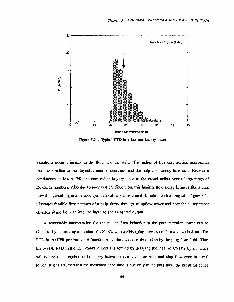
Chapter 3: MODELING AND SIMULATION OF A BLEACH PLANT
25
20
15
10
0 ----/I 0 15 20 25 30 35 ao
Time after Injection (min)
Figure 3.20: Typical RTD in a low consistency tower.
variations occur primarily in the fluid near the wall. The radius of this core section approaches
the tower radius as the Reynolds number decreases and the pulp consistency increases. Even at a
consistency as low as 2%, the core radius is very close to the vessel radius over a large range of
Reynolds numbers. Also due to poor vertical dispersion, this laminar flow slurry behaves like a plug
flow fluid, resulting in a narrow, symmetrical residence time distribution with a long tail. Figure 3.22
illustrates feasible flow patterns of a pulp slurry through an upflow tower and how the slurry tracer
changes shape from an impulse input to the measured output.
A reasonable interpretation for the unique flow behavior in the pulp retention tower can be
obtained by connecting a number of CSTR's with a PFR (plug flow reactor) in a cascade form. The
RTD in the PFR portion is a 5 function at tp, the residence time taken by the plug flow fluid. Thus
the overall RTD in the CSTRS+PFR model is formed by delaying the RTD in CSTRS by tp. There
will not be a distinguishable boundary between the mixed flow zone and plug flow zone in a real
tower. If it is assumed that the measured dead time is due only to the plug flow, the mean residence
45
46
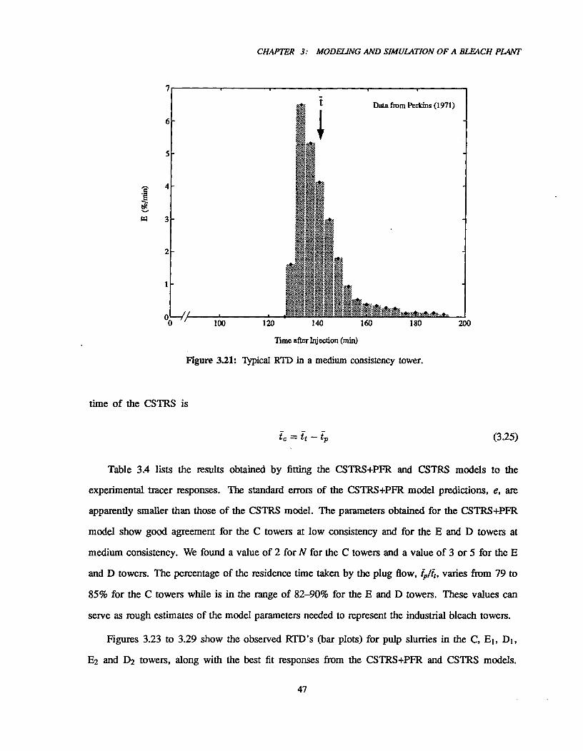
7
6
5
4
3
2
1
00-4/
Data from Perkins (1971)
100^120^140 160^180^200
CHAPTER 3: MODELING AND SIMULATION OF A BLEACH PLANT
Time after Injection (min)
Figure 3.21: Typical RTD in a medium consistency tower.
time of the CSTRS is
= —^ (3.25)
Table 3.4 lists the results obtained by fitting the CSTRS+PFR and CSTRS models to the
experimental tracer responses. The standard errors of the CSTRS+PFR model predictions, e, are
apparently smaller than those of the CSTRS model. The parameters obtained for the CSTRS+PFR
model show good agreement for the C towers at low consistency and for the E and D towers at
medium consistency. We found a value of 2 for N for the C towers and a value of 3 or 5 for the E
and D towers. The percentage of the residence time taken by the plug flow, ipat, varies from 79 to
85% for the C towers while is in the range of 82-90% for the E and D towers. These values can
serve as rough estimates of the model parameters needed to represent the industrial bleach towers.
Figures 3.23 to 3.29 show the observed RTD's (bar plots) for pulp slurries in the C, El, DI,
E2 and D2 towers, along with the best fit responses from the CSTRS+PFR and CSTRS models.
47
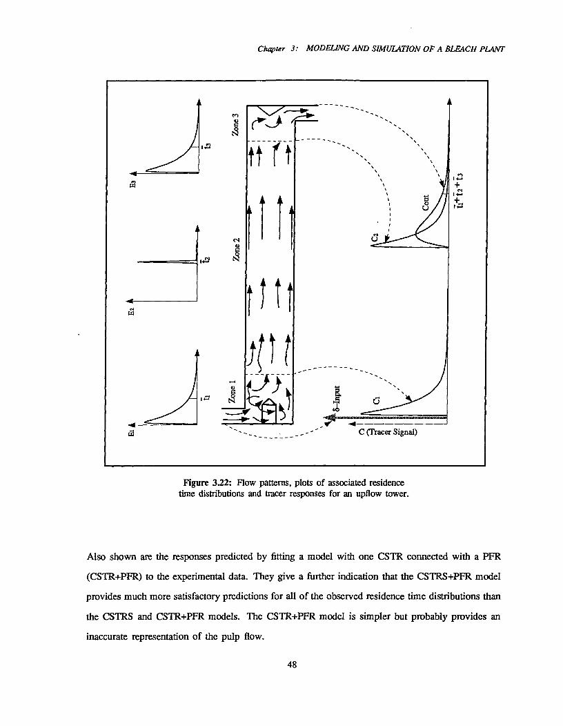
Chapter 3: MODELING AND SIMULATION OF A BLEACH PLANT
Figure 3.22: Flow patterns, plots of associated residencetime distributions and tracer responses for an upflow tower.
Also shown are the responses predicted by fitting a model with one CSTR connected with a PFR
(CSTR+PFR) to the experimental data. They give a further indication that the CSTRS+PFR model
provides much more satisfactory predictions for all of the observed residence time distributions than
the CSTRS and CSTR+PFR models. The CSTR+PFR model is simpler but probably provides an
inaccurate representation of the pulp flow.
48
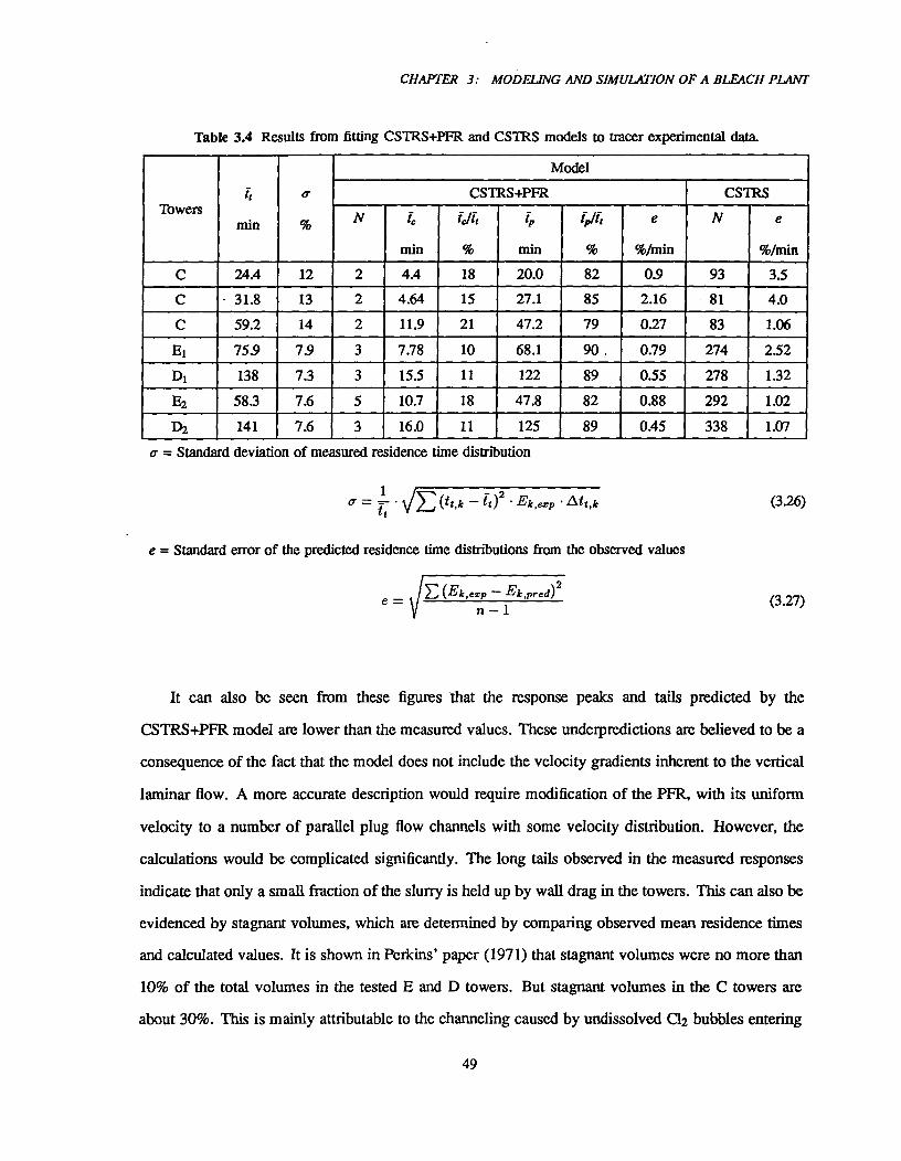
CHAPTER 3: MODELING AND SIMULATION OF A BLEACH PLANT
Table 3.4 Results from fitting CSTRS+PFR and CSTRS models to tracer experimental data.
Towersit
mm n
cr
%
Model
CSTRS+PFR CSTRS
N ic
Mill
idie
%
fP
min
tp/it
%
e
%/min
N e
%/min
C 24.4 12 2 4.4 18 20.0 82 0.9 93 3.5
C -^31.8 13 2 4.64 15 27.1 85 2.16 81 4.0
C 59.2 14 2 11.9 21 47.2 79 0.27 83 1.06
E1 75.9 7.9 3 7.78 10 68.1 90. 0.79 274 2.52
Di 138 7.3 3 15.5 11 122 89 0.55 278 132
E2 58.3 7.6 5 10.7 18 47.8 82 0.88 292 1.02
D2 141 7.6 3 16.0 11 125 89 0.45 338 1.07
o = Standard deviation of measured residence time distribution
0.= =...1 • vE^- it)2 Ek,exp • Ati,ktt
e = Standard error of the predicted residence time distributions from the observed values
VE (Ek,„ - Ek,pred)2
It can also be seen from these figures that the response peaks and tails predicted by the
CSTRS+PFR model are lower than the measured values. These underpredictions are believed to be a
consequence of the fact that the model does not include the velocity gradients inherent to the vertical
laminar flow. A more accurate description would require modification of the PFR, with its uniform
velocity to a number of parallel plug flow channels with some velocity distribution. However, the
calculations would be complicated significantly. The long tails observed in the measured responses
indicate that only a small fraction of the slurry is held up by wall drag in the towers. This can also be
evidenced by stagnant volumes, which are determined by comparing observed mean residence times
and calculated values. It is shown in Perkins' paper (1971) that stagnant volumes were no more than
10% of the total volumes in the tested E and D towers. But stagnant volumes in the C towers are
about 30%. This is mainly attributable to the channeling caused by undissolved C12 bubbles entering
e =n -1
(3.26)
(3.27)
49
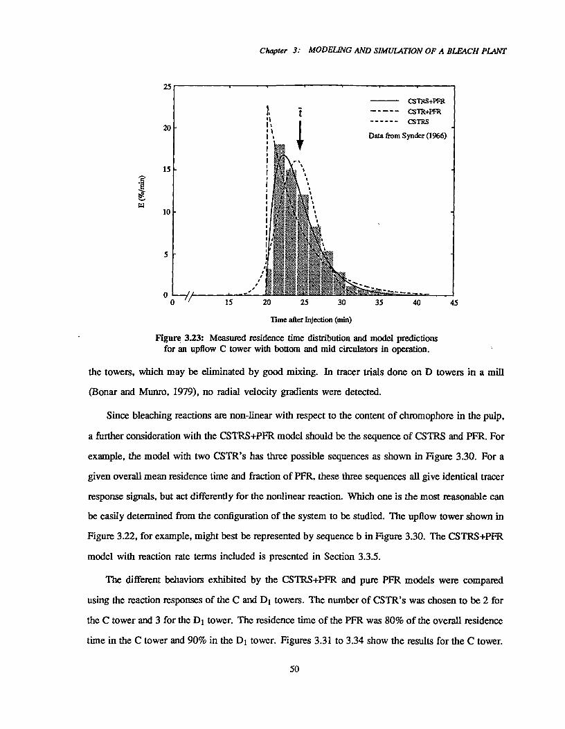
CSTRS+PFRCSTR+PFRCSTRS
Data from Synder (1966)ItIIi
-
Chapter 3: MODELING AND SIMULATION OF A BLEACH PLANT
25
20
15
1 0
5
15^20^25^30^35^ao^45
Time after Injection (min)
Figure 3.23: Measured residence time distribution and model predictionsfor an upflow C tower with bottom and mid circulators in operation.
the towers, which may be eliminated by good mixing. In tracer trials done on D towers in a mill
(Bonar and Munro, 1979), no radial velocity gradients were detected.
Since bleaching reactions are non-linear with respect to the content of chromophore in the pulp,
a further consideration with the CSTRS+PFR model should be the sequence of CSI'RS and PFR. For
example, the model with two CSTR's has three possible sequences as shown in Figure 3.30. For a
given overall mean residence time and fraction of PFR, these three sequences all give identical tracer
response signals, but act differently for the nonlinear reaction. Which one is the most reasonable can
be easily determined from the configuration of the system to be studied. The upflow tower shown in
Figure 3.22, for example, might best be represented by sequence b in Figure 3.30. The CSTRS+PFR
model with reaction rate terms included is presented in Section 3.3.5.
The different behaviors exhibited by the CSTRS+PFR and pure PFR models were compared
using the reaction responses of the C and DI towers. The number of CSTR's was chosen to be 2 for
the C tower and 3 for the DI tower. The residence time of the PFR was 80% of the overall residence
time in the C tower and 90% in the D1 tower. Figures 3.31 to 3.34 show the results for the C tower.
50
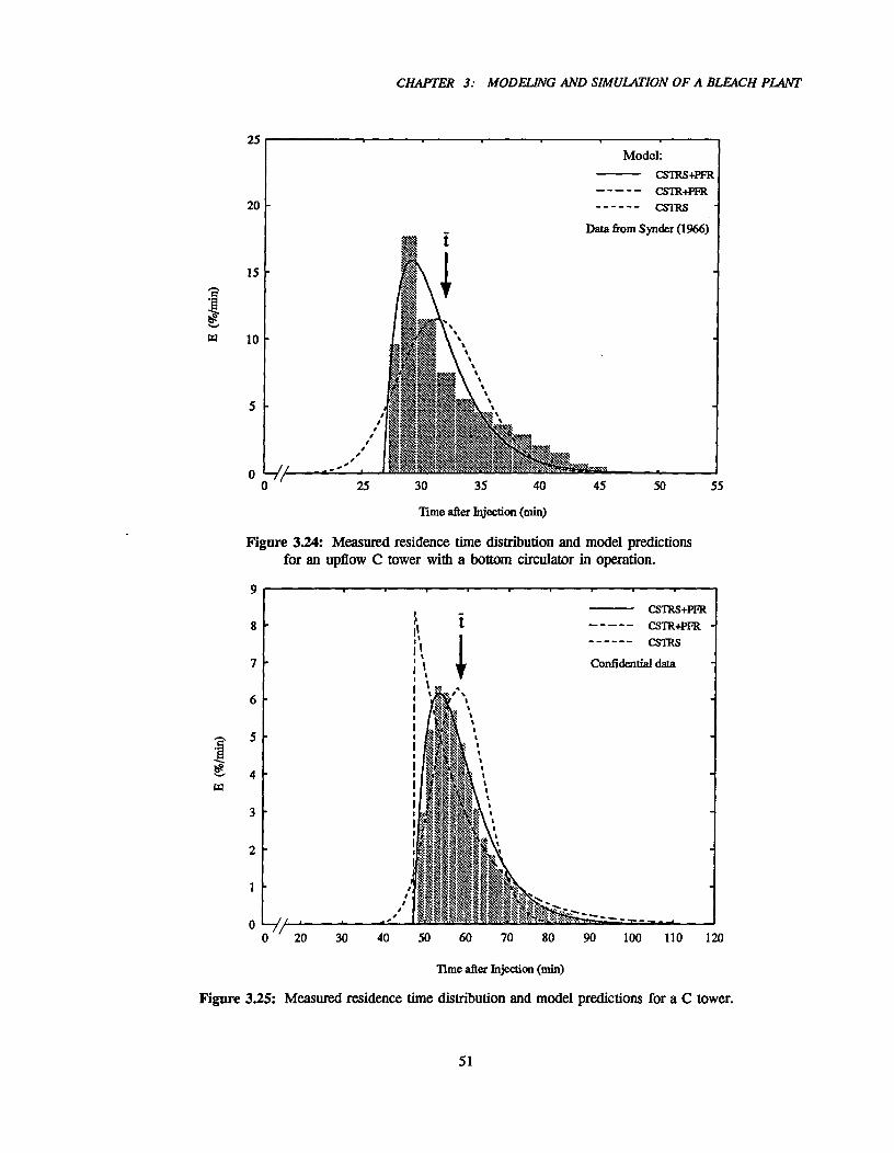
25
20
15
5
025^30^35^40^45^50^55
CSTRS+PFRCSTR+PFRCSTRS
Confidential data
9 ^
8
7
6
5
4
3
2
1
00^20 30^40^50^60
^70^80^90^100^110^120
CHAPTER 3: MODELING AND SIMULATION OF A BLEACH PLANT
lime after Injection (win)
Figure 3.24: Measured residence time distribution and model predictionsfor an upflow C tower with a bottom circulator in operation.
Tune after Injection (win)
Figure 3.25: Measured residence time distribution and model predictions for a C tower.
51

Chapter 3: MODELING AND SIMULATION OF A BLEACH PLANT
16
CSTRS+PFRCSTR+PFR
^ CSTRS -
Data from Perkins (1971)
10
8
6
4
2
70^80
lime after Injection (min)
Figure 3.26: Measured residence time distribution and model predictions for a downflow El tower.
II
III '
I'I'12
14
180-
150^160^170
CSTRS+PFRCSTR+PFRCSTRS
Data from Perkins (1971)
7
6
5
4
3
2
^t4. ^110^120^130^140
8
Time after Injection (min)
Figure 3.27: Measured residence time distribution and model predictions for an upflow D1 tower
52

CHAPTER 3: MODELING AND SIMULATION OF A BLEACH PLANT
14
12
10
8
6
4
2
Time after Injection (min)
Figure 3.28: Measured residence time distribution and model predictions for a downflow E2 tower.7
6
5
4
34.1
2
1
■,
,
o—//^_.....,'^st;_..,.,;.. ;,........^mwakt. s--..:,.774-,qp.,..,...9.....„ _ o^100^120^140^160^180^200
Time after Injection (min)
Figure 3.29: Measured residence time distribution and model predictions for an upflow D2 tower.
^ CSTRS+PFRCSTR+PFR
^ CSTRS^-Data from Perkins (1971)
53
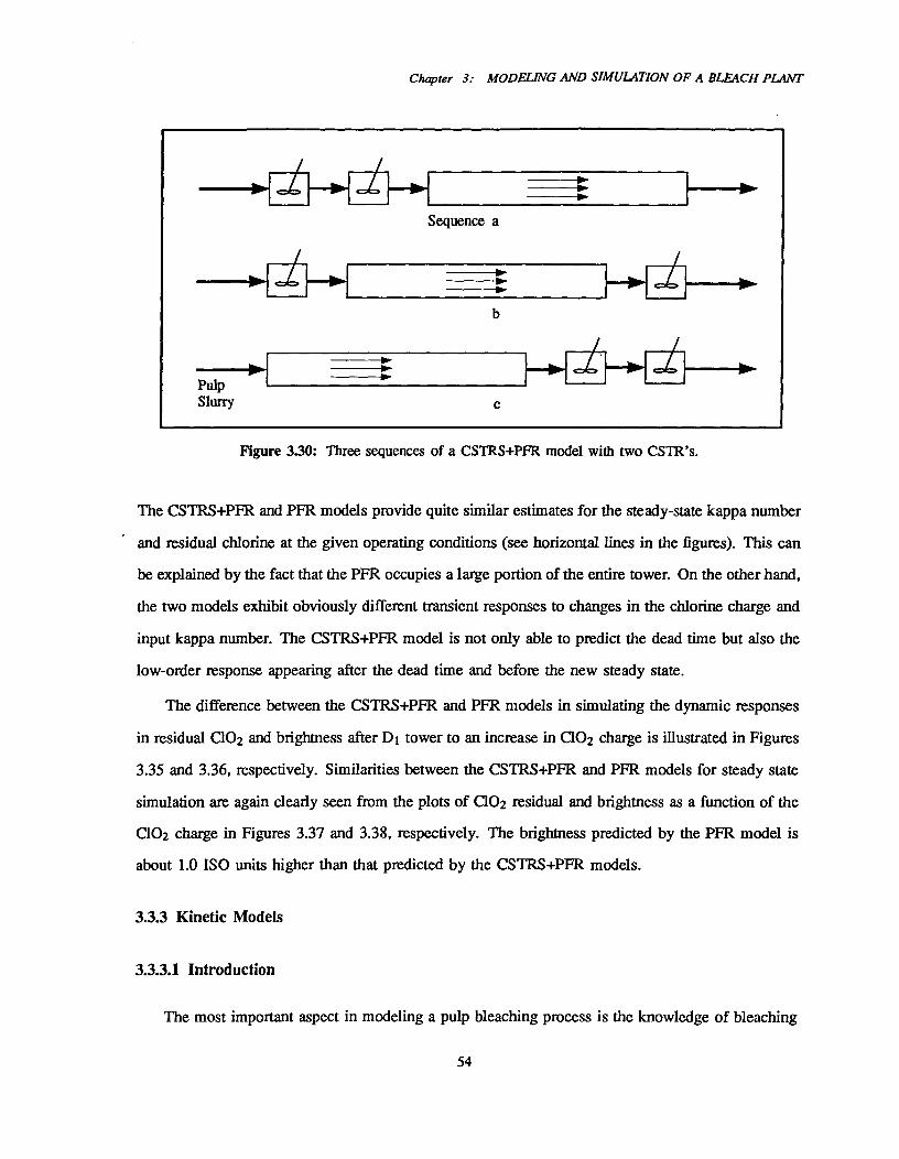
Chapter 3: MODELING AND SIMULATION OF A BLEACH PLANT
Figure 330: Three sequences of a CSTRS+PFR model with two CSTR's.
The CSTRS+PFR and PFR models provide quite similar estimates for the steady-state kappa number
and residual chlorine at the given operating conditions (see horizontal lines in the figures). This can
be explained by the fact that the PFR occupies a large portion of the entire tower. On the other hand,
the two models exhibit obviously different transient responses to changes in the chlorine charge and
input kappa number. The CSTRS+PFR model is not only able to predict the dead time but also the
low-order response appearing after the dead time and before the new steady state.
The difference between the CSTRS+PFR and PFR models in simulating the dynamic responses
in residual 002 and brightness after DI tower to an increase in 002 charge is illustrated in Figures
3.35 and 3.36, respectively. Similarities between the CSTRS+PFR and PFR models for steady state
simulation are again clearly seen from the plots of 002 residual and brightness as a function of the
002 charge in Figures 3.37 and 3.38, respectively. The brightness predicted by the PFR model is
about 1.0 ISO units higher than that predicted by the CSTRS+PFR models.
33.3 Kinetic Models
3.3.3.1 Introduction
The most important aspect in modeling a pulp bleaching process is the knowledge of bleaching
54
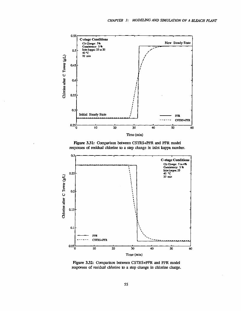
s ^
0.050 5010 20 30 40 60
0.3C -stage Conditions
Q2 Charge: 5 to 4%Consistency: 3%Inlet kappa: 2540°C32 min
0.25
0.1
PFRCSTRS+PFR
CHAPTER 3: MODELING AND SIMULATION OF A BLEACH PLANT
0.55
0.5
0.45
0.4
a 0.35
0.3 -
C-stage ConditionsC12 Charge: 5%Consistency: 3 %Inlet kappa: 25 to 2040°C32 min
Initial Steady State
New Steady State
PFRCSTRS+PFR
^0.25^
^
0^
10^20^30^40^50^60
Time (min)
Figure 331: Comparison between CSTRS+PFR and PFR modelresponses of residual chlorine to a step change in inlet kappa number.
Time (min)
Figure 332: Comparison between CSTRS+PFR and PFR modelresponses of residual chlorine to a step change in chlorine charge.
55
9.5
9
Chapter 3: MODELING AND SIMULATION OF A BLEACH PLANT
12
113
PFR
CSTRS+PFR
C-stage Conditionscli Charge: 5%Consistency: 3 %Inlet kappa: 25 to 2040°C32 min
10
Time (min)
Figure 3.33: Comparison between CSTRS+PFR and PFR model responsesof kappa number after C tower to a step change in inlet kappa number.
15.5
8.50 20 30 ao 50 60
15
g^14.5
14
13.5
eosk^13
4412.5
C-stage ConditionsCo Charge: 5 to 4%Consistency: 3%Inlet kappa: 2540°C32 min
12 PFR
CSTRS+PFR
11.50^10^20^30
Time (min)
Figure 334: Comparison between CSTRS+PFR and PFR model responsesof kappa number after C tower to a step change in chlorine charge.
40 50 60
56
0.85
0.8
0.75
Di-stage ConditionsC102 Charge: 1.2 to 1.4%
- Consistency: 10.9 %Inlet Brighteness: 37.570 °C
... 160 snin
i
F
fai^0.65
t^0.73o
_ - - - - - - - - - - - - - - - - -• • " .. --
• ..^-
C")I
0.45 -
0.55 - :
II
IIi
PFRCSTRS+PFR
0.4 --//0^ 160
Time (min)
Figure 3.35: Difference between CSTRS+PFR and PFR models responsesof residual chlorine dioxide to a step change in chlorine dioxide charge.
120 140 220180 200
73.5 -
75
*E§ 74.5on
r.' ^74
.0eao
CHAPTER 3: MODELING AND SIMULATION OF A BLEACH PLANT
76Di-stage ConditionsC102 Charge: 1.2 to 1.4%Consistency: 10.9%
75.5 - Inlet Hz:leanness: 37.570 °C160 min
PFRCSTRS+PFR
73-70 120^140^160^180^200
I•
•
220
I , • , .. .... ----------------------
, -
Time (mm)
Figure 3.36: Difference between CSTRS+PFR and PFR model responsesof brightness after DI tower to a step change in chlorine dioxide charge.
57
7205 1.5 2 2.5 3.53 4
79DI-stage Conditions
Consistency: 10.9 ToInlet Brighteness: 375
- 70°C160 min
78
77
76
75
74
73
Chapter 3: MODELING AND SIMULATION OF A BLEACH PLANT
33DI-stage Conditions
Consistaicy: 10.9 %Inlet Brighteness: 37570 °C160 min
1.5
1.0
03
1.5^2^2.5^3^3.5
C102 Charge (% on od pulp)
Figure 3.37: Comparison between CSTRS+PFR and PFR model predictionsof residual chlorine dioxide as a function of chlorine dioxide charge.
C102 Charge (% on od pulp)
Figure 3.38: Comparison between CSTRS+PFR and PFR model predictionof brightness after DI tower as a function of chlorine dioxide charge.
3.0
%55
58
CHAPTER 3: MODELING AND SIMULATION OF A BLEACH PLANT
reaction kinetics. In the process kinetic models employed in this study, the removal of chromophores
in the pulp is characterized by a decrease in the kappa number for delignification reactions and by
a decrease in the light absorption coefficient for brightening reactions.
After a comprehensive survey, we found that research in this area has not caught up with the
rapid changes in pulp bleaching technology. It was difficult to evaluate and use the kinetic models
for delignification with chlorine dioxide alone or with mixture of chlorine dioxide and chlorine
developed by Germgird et al. (Germgard et al., 1982; Germgird and Lindberg, 1982) since neither
the parameters nor the experimental data supporting the models were published. Furthermore, the
(C+D) model is only valid for a simultaneous addition of chlorine dioxide and chlorine whereas
sequential charges are usually employed in a modem chlorination stage. There has been no kinetic
model published to describe Eo bleaching, which is another modification in bleaching 'craft pulp.
An empirical model by Mackinnon (1987) failed to produce a representation of the Eo bleaching
reaction rate although it is called a kinetic model by the author. Due to these circumstances, only
kinetic models for the C, Er, DI, E2 and D2 stages are incorporated in this study. As the kinetics
of these bleaching reactions were largely studied by laboratory experiments with constant chemical
compositions, low fibre consistencies and good mixing, the experimental conditions may not be
similar to mill scale practice. The experimental conditions and pretreatment on which the models are
based are shown in Table 3.5. The table also gives the ranges for which the models are applicable.
The type of pretreatment has a pronounced effect on the reactivity of the pulp towards the chemicals.
333.2 Chlorine Delignification
Of the kinetic models proposed by several authors for chlorine bleaching, one by Ackert et al.
(1973) is identified as a combination of simplicity and accuracy. This model divides the lignin into
three types: fast, slow and a floor level or unreactive lignin. The rate of fast lignin removal is given by
= ki • [C12] • Kai^ (3.28)
while the rate of slow lignin removal is
dKa2^r" 1 r'T2 = -^= &2 • 1%-,121di(3.29)
dKai= - dt
59
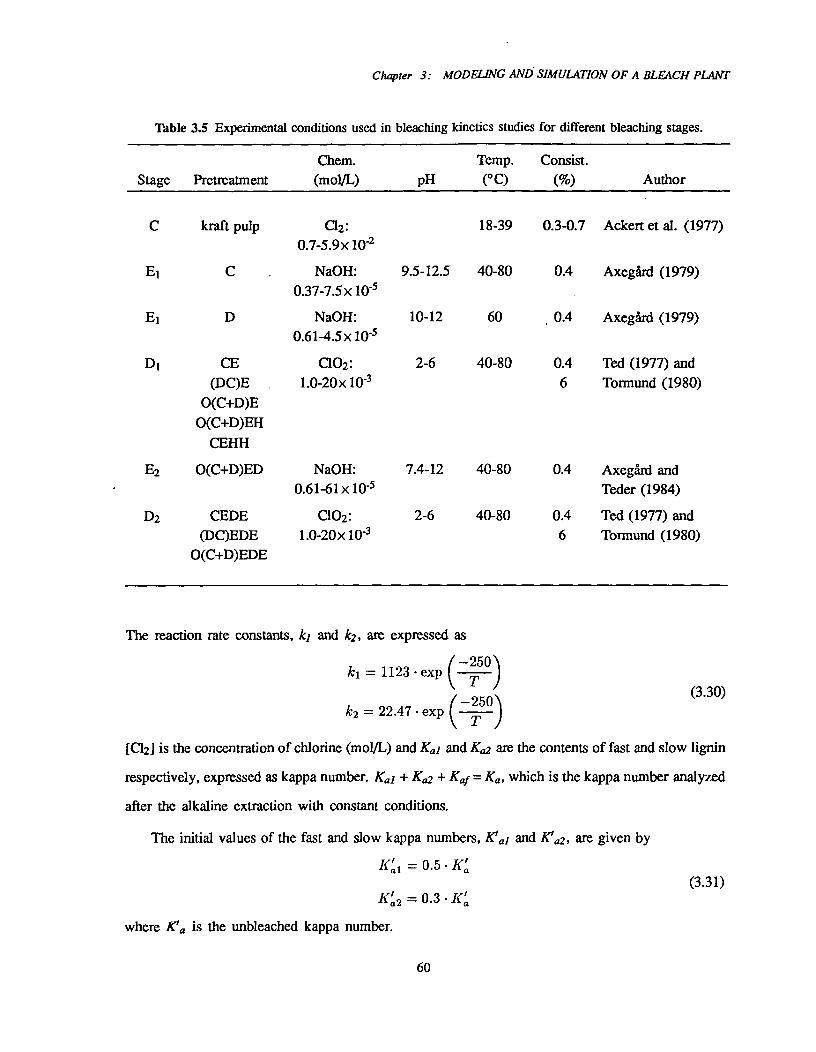
Chapter 3: MODELING AND SIMULATION OF A BLEACH PLANT
Table 3.5 Experimental conditions used in bleaching kinetics studies for different bleaching stages.
Stage PretreatmentChem.
(mol/L) pHTemp.(0
Consist.(%) Author
kraft pulp C12: 18-39 0.3-0.7 Ackert et al. (1977)0.7-5.9x 10⁻²
E1 NaOH: 9.5-12.5 40-80 0.4 Axegfird (1979)0.37-7.5x 10⁻⁵
E1 NaOH: 10-12 60 , 0.4 Axegfird (1979)0.61-4.5x 10⁻⁵
DI CE C102: 2-6 40-80 0.4 Ted (1977) and(DC)E 1.0-20x 10-3 6 Tormund (1980)
0(C+D)E0(C+D)EH
CEHH
E2 0(C+D)ED NaOH: 7.4-12 40-80 0.4 Axegird and0.61-61x 10-5 Teder (1984)
D2 CEDE C102: 2-6 40-80 0.4 Ted (1977) and(DC)EDE 1.0-20x 10-3 6 Tormund (1980)
0(C+D)EDE
The reaction rate constants, ki and k2, are expressed as
( :1_7,250)ki = 1123 .exp
T250)k2 = 22.47•exp
(3.30)
[C12] is the concentration of chlorine (mol/L) and Kai and Ka2 are the contents of fast and slow lignin
respectively, expressed as kappa number. Kai + Ka2 + K01= Ka, which is the kappa number analyzed
after the alkaline extraction with constant conditions.
The initial values of the fast and slow kappa numbers, lea] and ra2, are given by
= 0.5(3.31)
Kai 2 = 0.3 • K
where K'0 is the unbleached kappa number.
60

= Wu,Kappa number decreaseC12 consumption, % on od pulp
CHAPTER 3: MODELING AND SIMULATION OF A BLEACH PL41VT
The stoichiometric relationship between chlorine consumption and decrease in kappa number is
(3.32)
where Wm, is the stoichiometric coefficient (rs, 0.208).
Hydrogen ions are formed during the chlorination. If it is assumed that the substitution reaction
- is the fast reaction and the oxidation reaction is the slow one, then each mole of reacted C12 produces
one and two moles of H+, respectively, for the fast and slow reactions.
The kinetics of chlorine bleaching with low C102 substitution are assumed to be the same as for
C12 bleaching. Then, the total chlorine concentration includes chlorine dioxide as active chlorine. 1
kg C102 is equivalent to 2.63 kg chlorine based on their oxidizing power.
3.3.3.3 First Alkaline Extraction
The reaction kinetics and lignin solubilization mechanism during the first extraction stage are
poorly understood. This lack of understanding is reflected by the fact that only three attempts at
modelling delignification kinetics have been published, by AxegArd (1979), Mackinnon (1987) and
Taylor et al. (1982). Axegard's model has some fundamental basis while Taylor's is completely
empirical. Mackinnon continued Axegfird's work but did not obtain any significant improvement.
AxegArd's model was tested and modified in the present study. Kinetic data bases published by
AxegArd, including experimental conditions and results for extracting chlorine bleached pulp and
chlorine dioxide bleached pulp, are shown in Table 3.6 and Table 3.7, respectively.
AxegArd's model represents extraction of the chlorine bleached pulp by two parallel first-order
reactions with respect to kappa number decrease: one is the fast lignin reaction and the other is the
slow lignin reaction. The rates of these dtwoireactions are expressed as followsK
rl -dKdat2
ki • [0111 "Kai
r2 = - = k2 • [OH-]0.05 Ka2
dt
where Kai and Ka are fast and slow kappa numbers respectively and [OM is hydroxyl ion
concentration (moVL). ki and k2 are the rate constants of the fast and slow reactions respectively.
(3.33)
61
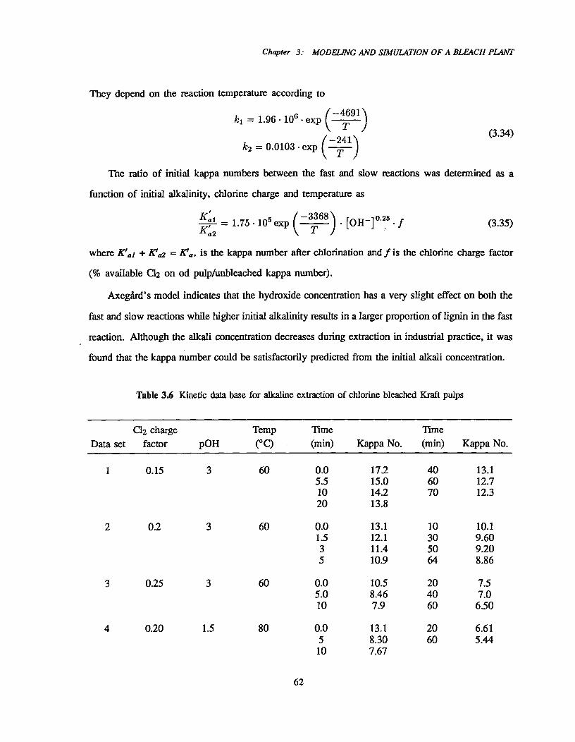
Chapter 3: MODELING AND SIMULATION OF A BLEACH PLANT
They depend on the reaction temperature according to
-4691)k1 = 1.96 • 106 • exp ^T
-241)k2 = 0.0103 exp(3.34)
The ratio of initial kappa numbers between the fast and slow reactions was determined as a
function of initial alkalinity, chlorine charge and temperature as
-1,,,C; 102^
)= 1.75.^ 1-3368"105 exp ^[011-}a25-f'
(3.35)
where K'01 + ra2 = ra, is the kappa number after chlorination and f is the chlorine charge factor
(% available C12 on od pulp/unbleached kappa number).
Axegird's model indicates that the hydroxide concentration has a very slight effect on both the
fast and slow reactions while higher initial alkalinity results in a larger proportion of lignin in the fast
reaction. Although the alkali concentration decreases during extraction in industrial practice, it was
found that the kappa number could be satisfactorily predicted from the initial alkali concentration.
Table 3.6 Kinetic data base for alkaline extraction of chlorine bleached Kraft pulps
Data setC12 charge
factor p0HTemp(°c)
Time(min) Kappa No.
Time(min) Kappa No.
1 0.15 3 60 0.0 172 40 13.15.5 15.0 60 12.710 14.2 70 12.320 13.8
2 0.2 3 60 0.0 13.1 10 10.11.5 12.1 30 9.603 11.4 50 9.205 10.9 64 8.86
3 0.25 3 60 0.0 10.5 20 7.55.0 8.46 40 7.010 7.9 60 6.50
4 0.20 1.5 80 0.0 13.1 20 6.615 8.30 60 5.4410 7.67
62
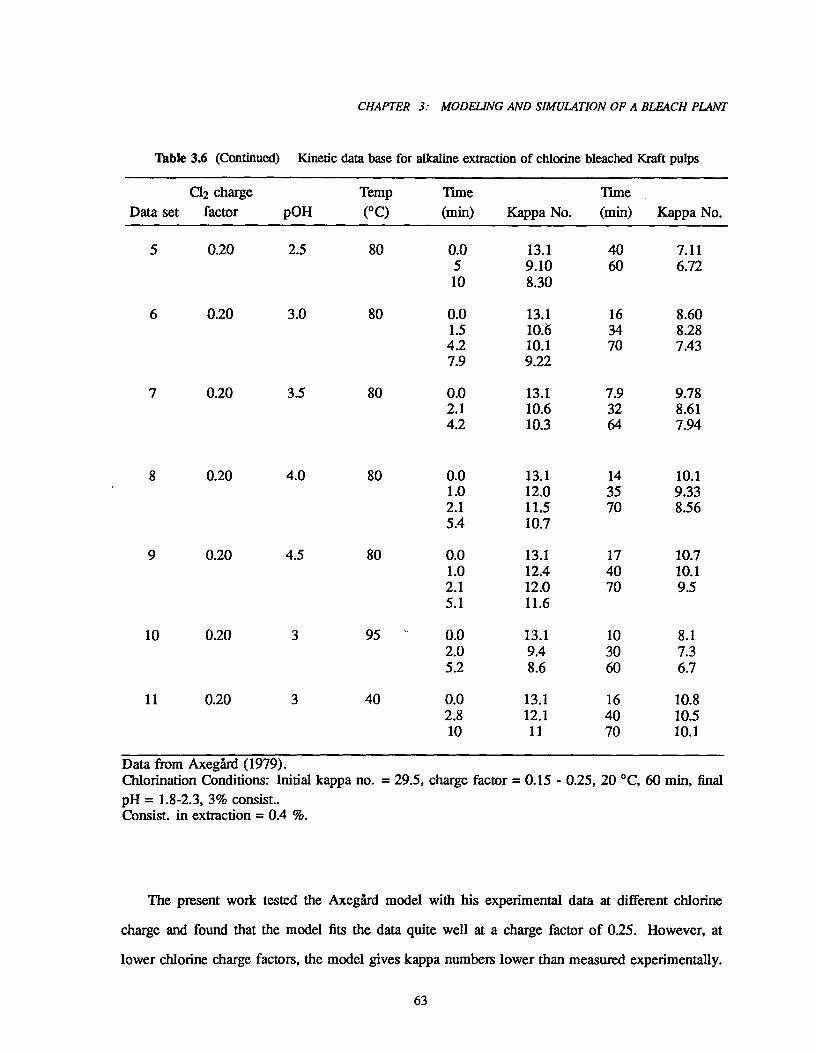
Table 3.6 (Continued)
CHAPTER 3: MODELING AND SIMULATION OF A BLEACH PLANT
Kinetic data base for alkaline extraction of chlorine bleached Kraft pulps
02 chargeData set^factor p0H
Temp(°C)
Time(min) Kappa No.
Time(min) Kappa No.
5 0.20 2.5 80 0.0 13.1 40 7.115 9.10 60 6.7210 8.30
6 0.20 3.0 80 0.0 13.1 16 8.601.5 10.6 34 8.2842 10.1 70 7.437.9 9.22
7 0.20 3.5 80 0.0 13.1 7.9 9.782.1 10.6 32 8.614.2 10.3 64 7.94
8 0.20 4.0 80 0.0 13.1 14 10.11.0 12.0 35 9.332.1 11.5 70 8.565.4 10.7
9 0.20 4.5 80 0.0 13.1 17 10.71.0 12.4 40 10.12.1 12.0 70 935.1 11.6
10 0.20 3 95 0.0 13.1 10 8.12.0 9.4 30 7.35.2 8.6 60 6.7
11 0.20 3 40 0.0 13.1 16 10.82.8 12.1 40 10.510 11 70 10.1
Data from Axegard (1979).Chlorination Conditions: Initial kappa no. = 29.5, charge factor = 0.15 - 0.25, 20 °C, 60 min, finalpH = 1.8-2.3, 3% consist..Consist. in extraction = 0.4 %.
The present work tested the Axegard model with his experimental data at different chlorine
charge and found that the model fits the data quite well at a charge factor of 025. However, at
lower chlorine charge factors, the model gives kappa numbers lower than measured experimentally.
63
—3368)al = 2.72 10 • exp T 4^ [01110.25K' 2
(3.37)
Chapter 3: MODELING AND SIMULATION OF A BLEACH PLANT
This discrepancy increases as the chlorine charge decreases. The original model assumes that the
intensity of chlorination influences the initial distribution between the fast and slow kappa numbers
instead of the reaction rates. A more reasonable implication for the effect of chlorination intensity
could be that the rate of lignin solubilization will be slower in both the fast and slow reactions if
the pulp is treated with less chlorine. The modification of Axegfird's model proposed in this work
assumes that the reaction constants are proportional to the chlorine charge factor but the ratio of
initial kappa numbers is not dependent on chlorination intensity. By fitting the experimental data,
the new reaction constants are determined as
—4691
^
= 9.78 • 106 • exp ^f
—241
^
k2 = 0.0515 • exp^f(3.36)
and the ratio of initial kappa number as
Table 3.7 Kinetic data base of alkaline extraction for chlorine dioxide bleached Kraft pulps
Data set p0HTime(min) Kappa No.
Time(min) Kappa No.
1 2 0.0 15 20 1122.2 12.8 60 10.75 12.1 120 10.1
2 3 2.2 13.8 20 12.65 13.5 60 11.910 13.0 120 11.3
3 4 10 13.63 120 12.360 12.85
Data from Axegird (1979).Chlorination Conditions: Initial kappa no. = 29.5, charge factor = 0.14, 20 °C, 60 min, 3 % consist.,final pH = 2.0.Extraction Conditions: 60 °C, 0.4 % consist.
64

50 60 70 80
18
16
14
Z 12
10
8
6
40 10^20^30^40
Time (min)
— Our Modified Model- Axegard Model
o Experiment
CHAPTER 3: MODELING AND SIMULATION OF A BLEACH PLANT
Figure 3.39: Kappa number during E1 bleaching of chlorine bleachedpulps as calculated by our modified model and Axegard's model.
Figure 3.39 shows a comparison between our modified model and the original Axegird's model
for fitting the kappa number during the alkaline extraction of different chlorinated pulps. The modified
model represents the experimental data better than the original model when the chlorine charge factor
is reduced. A better fit of the overall data base is also achieved; the modified model yielded a standard
deviation of 0.6% compared to 0.8% for the original model. A further comparison is performed using
the experimental results of Histed et al. (1985), as shown in Table 3.8, which were obtained over
a wider range of chlorine charges. The modified model gives a much better prediction of Histed's
data than Axegdrd's model. This suggests that the present description of the reaction dependence on
chlorination intensity is more reliable. However, at chlorine charge factors beyond the range covered
by the model data base, the model predictions are slightly poorer. This occurs probably because there
is a complicated relationship between the extraction reaction rates and the charge factor. The linear
correlation assumed in the model is an approximation which is only valid within a narrow range.
65

Chapter 3: MODELING AND SIMULATION OF A BLEACH PLANT
Table 3.8 Comparison between our modified model and AxegArd model.
Cl2 chargefactor
C kappaNo.
CE Kappa No.
Experimental Predicted by ourmodified model
Predicted byAxegfird
0.16 16.1 6.1 6.1 5.702 13.0 4.8 4.7 4.1
0.22 10.5 3.7 3.7 3.10.26 7.7 3.0 2.6 2.10.29 6.0 2.6 1,9 1.50.32 5.0 1.9 1.5 1.2
Data from Histed et al (1985).C-Stage Conditions: Initial kappa no. = 30.4, 40-80 °C, 2.5% consist., time = to zero residual.E-Stage Conditions: 80 °C, 10% consist., 60 mm, NaOH charge = 3% on pulp
The two kinetic models were also compared for extraction of a chlorine dioxide bleached pulp
using the data base in Table 3.7. Good agreement between prediction of the modified model and
the experimental data was obtained if the reaction rate constants were adjusted to a lower value than
CE bleaching while the other model parameters were kept the same. The reaction mechanisms and
factors governing delignification rates seem to be the same in the extraction stage for both chlorine and
chlorine dioxide bleached pulps. Axegárd's suggestion for DE bleaching was that the initial fast-slow
ratio Kfai/IV.2 was higher than for CE bleaching. Shown in Figure 3.40 is the kappa number predicted
by the modified and original AxegArd's models for the extraction of a chlorine dioxide bleached pulp
at different alkali concentrations. It is clear that Axegfird's model is not applicable in this case.
33.3.4 Chlorine Dioxide Bleaching
Ted and Tormund (1977; 1980) represented the kinetic characteristics of the first and second
chlorine dioxide stages by the following equations:
r = -dKk
= k [C1021" • [WIT" k - K k f)3^(3.38)dt
with- Ea)
k = A1 • (K72 + A2) • exP^• 71)(3.39)
66

CHAPTER 3: MODELING AND SIMULATION OF A BLEACH PLANT
14
16 — Our Modified Model- -. Axegard Model
o Experiment
12
6
4
20^20^40^60
Time (min)
Figure 3.40: Kappa number during Ei bleaching of a chlorine dioxidebleached pulp as calculated by our modified model and AxegArd's model.
where Kk is the content of chromophores in the pulp expressed as the light absorption coefficient at
457 um (m2/kg), Kji is the floor level of Kk (r4.1 m2/kg), [C102] is the mole concentration of C102,
[R] is the mole concentration of 11+, E. is the activation energy (rs,59 kJ/mol) and ICI is the initial
Kk value. The constants Ai and A2 are dependent of the type of prebleaching (see Table 3.9).
Table 3.9 Rate constants A1 and A2 for C102 bleaching for different pulps.
Prebleaching A1 A2
(DC)E 0.145x 10¹⁰ -0.435x 10⁻³(DC)EDE 0.117x10⁹ 0.01
0(C+D)EH 0.096x 10⁹ 0.023
Data from Ted and Tormund (1980)
80^100^120
67

Chapter 3: MODELING AND SIMULATION OF A BLEACH PLANT
Stoichiometric constants n and A3 for C102 consumption in C102 bleaching for different pulps.
Prebleaching A3
0(C+D)E 1.3 0284
CEHH 1.6 0.486
(DC)E 1.0 0.292
0(C+D)EH 1.15 0.398
(DC)EDE 2.5 0.527K'k
0(C+D)EDE 2.0 0.0675ICk
Data from Ted and Tormund (1980)
The stoichiometric relationship for C102 consumption is
C102 consumption, % on od pulp1= A 3 • — = Tcio2Light absorption coefficient decrease Kk
(3.40)
and for II+ generation is
11+ generation, % on od pulp
(3.41)
H+Light absorption coefficient decrease =
where n and A3 vary with pulp type, as listed in Table 3.10. In most cases, 1F H+ was found to be
directly proportional to Tao, independent on pH, pulp type and temperature.
The rate and stoichiometric constants for chlorine dioxide bleaching of the (DC)E prebleached
pulp in Tables 3.9 and 3.10 were used in the DI stage for simulation of a CDEDED sequence in this
work. The kinetic constants used for the D2 stage are discussed below.
3.3.3.5 Second Alkaline Extraction
Axegard and Teder (1984) found that the E2 stage itself can not delignify or brighten pulp, as
is the case for the El stage. The main effects of the E2 stage are to improve the reactivity of pulp
and to decrease the C102 consumption in the subsequent D2 stage. The bleaching efficiency of the
D2 stage can be increased by higher alkalinity, higher temperature or longer reaction time in the E2
stage. To account for the effects of E2 conditions on D2 bleaching kinetics, we have correlated the
Table 3.10
68
CHAPTER 3: MODELING AND SIMULATION OF A BLEACH PLANT
rate and stoichiometric constants for D2 bleaching with E2 conditions on the basis of Axegard and
Teder's investigation, to obtain
A2 = B1 • [0111" • • exp ( ------RE. T
ai)
Ea2A3 = B2 • [OH 1-1 1°8 • exp (-7----R • T
)
(3.42)
(3.43)
where [OM, tr and T are the alkalinity, reaction time and temperature, respectively, in the E2 stage
while A2 and A3 are the rate constant in Equation 3.39 and the stoichiometric constant in Equation
3.40 respectively, for the D2 stage. The constants in Equation 3.42 and 3.43 were determined to be:
B./ = 9.1x 10¹²
B2 = 0.02
Ea/ = 15 kJ/mol
Ea2 = —8 kJ/mol
3.3.4 Correlation of Light Absorption Coefficient with Kappa Number after the E1 Stage
Kappa number is a chemical method which indicates the content of lignin in pulp during the
delignification phase while the light absorption coefficient is an optical measurement which indicates
the content of chromophores in pulp during the brightening phase. Norrstrtim (1972) has shown that a
theoretical relationship exists between the absorption coefficient of pulp and the contents of different
chemical species responsible for the pulp color. But none attempted to quantitatively correlate the
light absorption coefficient with the lignin content or kappa number of a bleached pulp. A linear
relationship between the light absorption coefficient and the kappa number was employed in this work
in order to simulate the complete bleach plant and to study how changes in the early delignification
stages transfer to the later brightening stages. It was derived from the theory (NorrstrOm, 1972)
that the light absorption coefficient of pulp is directly proportional to the content of chromophores
in the pulp:
Kk = E Kki • Ci^ (3.44)i
69
Chapter 3: MODELING AND SIMULATION OF A BLEACH PLANT
where Ci is the content of chromophore species i (mass percentage in pulp) and Kki is its specific
absorption coefficient (m2/kg). Since elimination of chromophores in the delignification phase is
accomplished by removal of lignin, it is possible that the lignin content represents the chromophore
content for a delignified pulp. Thus, Equation 3.44 can be rewritten as
Kk = KkLI • CLI b (3.45)
where the subscript LI denotes lignin and b represents the contribution from the other components
of pulp such as extractives and carbohydrates. It is assumed that b has a very small value compared
to the product KkIA • Cm because lignin is the main contributor to the light absorption of pulp.
Furthermore, based on the fact that the kappa number is directly proportional to the lignin content,
it is assumed that a linear relationship exists between the light absorption coefficient and the kappa
number for the pulp after the E1 stage, i.e.,
Kk = a Ka + b (3.46)
As the nature of the chromophoric groups in pulp is not well known, the values of a and b can not
be theoretically estimated. They were obtained by fitting experimental data. Experimental data for
the light absorption coefficient versus the kappa number were not directly available in the literature,
but were calculated from corresponding brightness values using the Kubellca-Munk equation:
Kk (1 — RoofS — 2 Roc,
(3.47)
where Roo denotes the reflectance of the pulp sheet to blue light at a 475 nm wavelength, i.e., the
brightness. S, the light scattering coefficient, depends on the physical structure of the pulp sheet; it
varies from 30 m2/kg for a thin sheet of kraft pulp to 50 m2/kg for a thick one (Teder and Tormund,
1977; 1980). In this work, a scattering coefficient value of 50 m2/kg was used to convert brightness
values to light absorption coefficients or vice versa. An average value should be obtained from
experimental data when simulating a given bleach plant.
Table 3.11 shows the data base for the brightness versus kappa number results reported by
Liebergott (1991) and Dubelsten (1992). The corresponding light absorption coefficients calculated
70
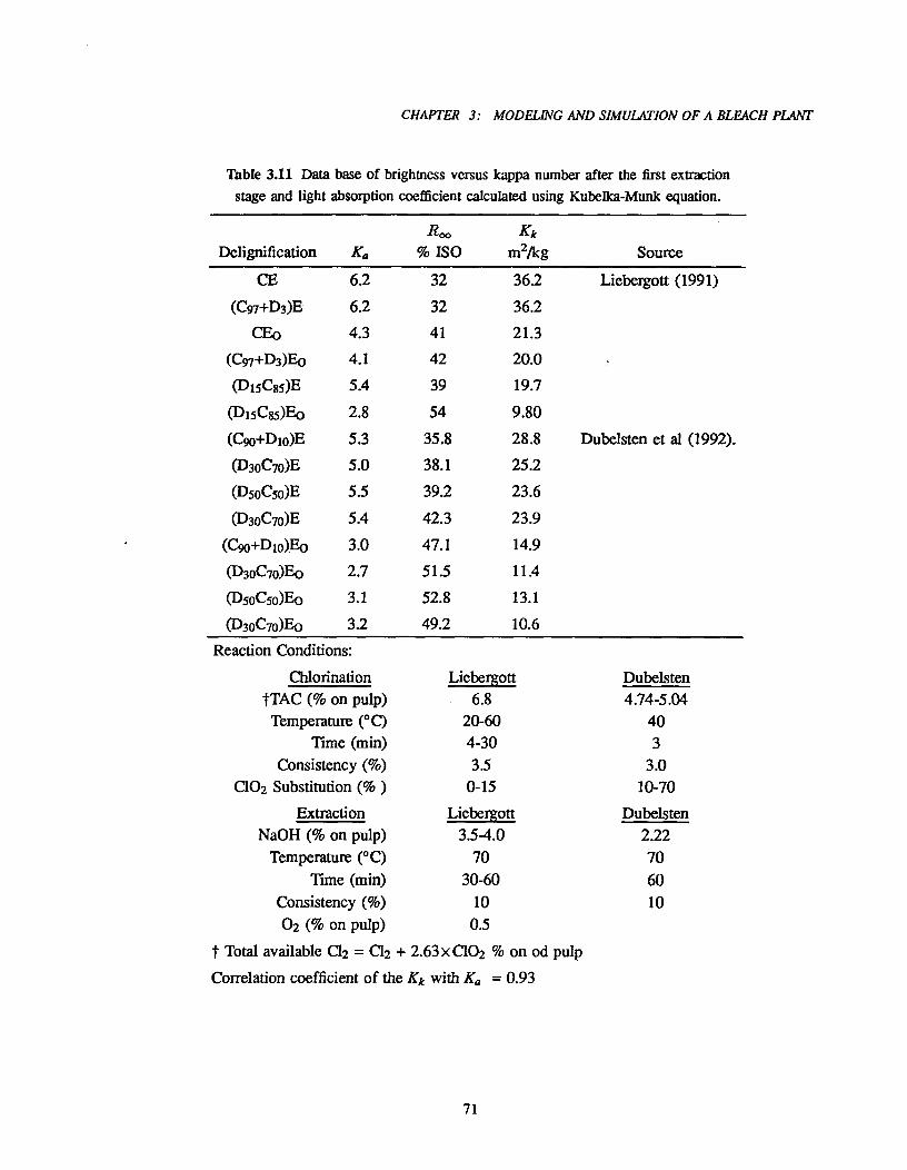
CHAPTER 3: MODELING AND SIMULATION OF A BLEACH PLANT
Table 3.11 Data base of brightness versus kappa number after the first extractionstage and light absorption coefficient calculated using Kubelka-Munk equation.
Delignification KaRao
% ISOKk
m2/kg Source
CE 62 32 362 Liebergott (1991)(C97+D3)E 6.2 32 36.2
CE0 4.3 41 21.3(C97+D3)E0 4.1 42 20.0
(D 15 C85)E 5.4 39 19.7
(315C85)E0 2.8 54 9.80
(C90+1310)E 5.3 35.8 28.8 Dubelsten et al (1992).
()30070)E 5.0 38.1 25.2
(350050)E 5.5 39.2 23.6
()30070)E 5.4 42.3 23.9(C90+D1o)E0 3.0 47.1 14.9
(D30070)E0 2.7 51.5 11.4
(1350050)E0 3.1 52.8 13.1
(D30C70)Eo 3.2 49.2 10.6Reaction Conditions:
Chlorination Liebergott DubelstentTAC (% on pull)) 6.8 4.74-5.04Temperature (°C) 20-60 40
Time (min) 4-30 3Consistency (%) 3.5 3.0
C102 Substitution (% ) 0-15 10-70Extraction Liebergott Dubelsten
NaOH (% on pulp) 3.5-4.0 2.22Temperature (°C) 70 70
Time (min) 30-60 60Consistency (%) 10 1002 (% on Pulp) 0.5
t Total available C12 = C12 + 2.63x C102 % on od pulpCorrelation coefficient of the Kk with Ka = 0.93
71
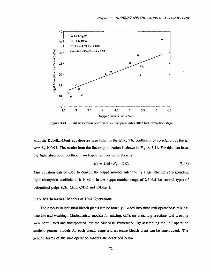
5.5 6.56
40
35
30
25
20
10
52.5^3^3.5^4^4.5^5
Chapter 3: MODELING AND SIMULATION OF A BLEACH PLANT
Kappa Number after Et Stage
Figure 3.41: Light absorption coefficient vs. kappa number after first extraction stage.
with the Kubelka-Munk equation are also listed in the table. The coefficient of correlation of the Kk
with Ka is 0.93. The results from the linear optimization is shown in Figure 3.41. For this data base,
the light absorption coefficient — kappa number correlation is
Kk = 4.69 K a + 0.01 (3.48)
This equation can be used to convert the kappa number after the El stage into the corresponding
light absorption coefficient. It is valid in the kappa number range of 2.5-6.5 for several types of
delignified pulps (CE, CE0, C/DE and C/DE0 ).
33.5 Mathematical Models of Unit Operations
The process in industrial bleach plants can be broadly divided into three unit operations: mixing,
reaction and washing. Mathematical models for mixing, different bleaching reactions and washing
were formulated and incorporated into the SIMNON framework. By assembling the unit operation
models, process models for each bleach stage and an entire bleach plant can be constructed. The
generic forms of the unit operation models are described below.
72
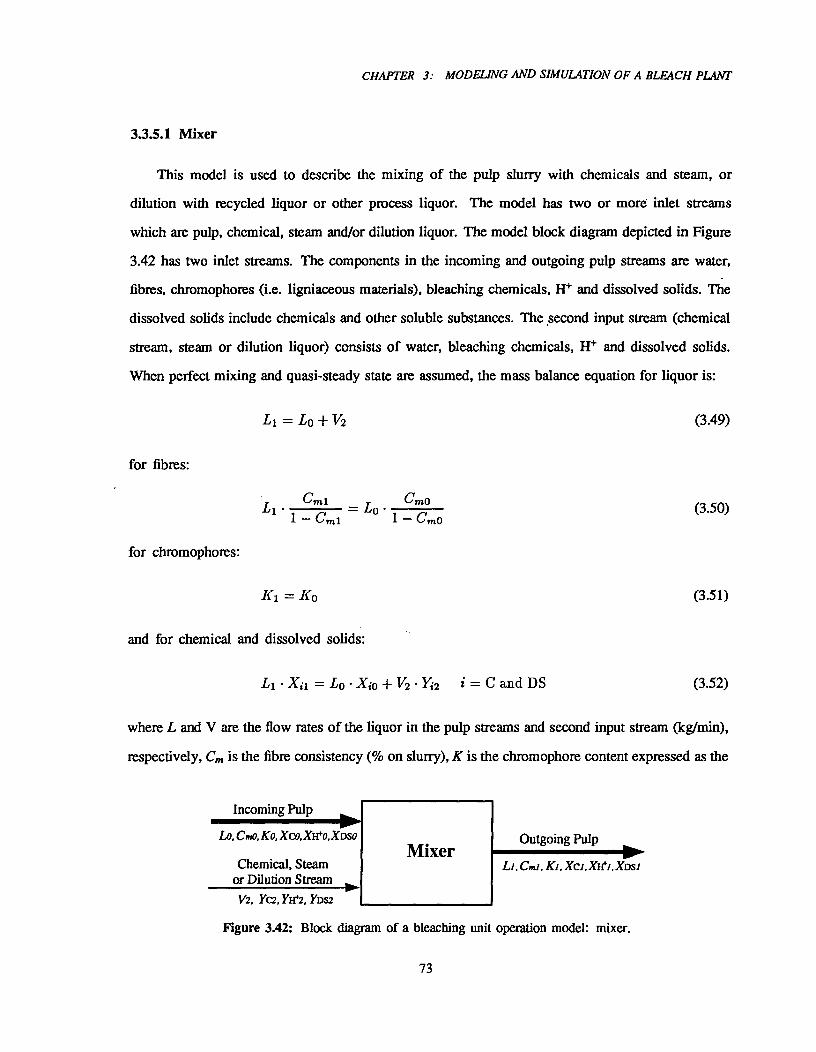
CHAPTER 3: MODELING AND SIMULATION OF A BLEACH PLANT
33.5.1 Mixer
This model is used to describe the mixing of the pulp slurry with chemicals and steam, or
dilution with recycled liquor or other process liquor. The model has two or more inlet streams
which are pulp, chemical, steam and/or dilution liquor. The model block diagram depicted in Figure
3.42 has two inlet streams. The components in the incoming and outgoing pulp streams are water,
fibres, chromophores (i.e. ligniaceous materials), bleaching chemicals, H+ and dissolved solids. The
dissolved solids include chemicals and other soluble substances. The second input stream (chemical
stream, steam or dilution liquor) consists of water, bleaching chemicals, H+ and dissolved solids.
When perfect mixing and quasi-steady state are assumed, the mass balance equation for liquor is:
LI = LO + V2^ (3.49)
for fibres:
Cm,i^CmoLi ^ --= Lo ^1— Cmi^1 — Cmo
for chromophores:
= Ko
and for chemical and dissolved solids:
Li • Xii = Lo Xio + V2 • Yi2
(3.50)
(3.51)
i = C and DS^(3.52)
where L and V are the flow rates of the liquor in the pulp streams and second input stream (kg/min),
respectively, Cm is the fibre consistency (% on slurry), K is the chromophore content expressed as the
Incoming Pulp
Chemical, Steamor Dilution Stream
01"Mixer
Outgoing Pulp ow
LI ,Cml , KI, XCI,X}f1,XDS1
Lo,Cmo,Ko, Xco,Xxio,XDso
V2, YC2, YH42, YDS2
Figure 3.42: Block diagram of a bleaching unit operation model: mixer.
73
Chapter 3: MODELING AND SIMULATION OF A BLEACH PLANT
kappa number or the light absorption coefficient, and Xi and Yi represent the contents of the chemical
and dissolved solids in the pulp streams and second input stream (% on liquor), respectively.
To determine the outlet H+ content, the following reaction is considered:
H+ + OH- H20^ (3.53)
The governing equilibrium relationship is
17. [OH-] [H+] 17 x KwXOH- • XH+^2 pf
(3.54)
where X0H- and XH+ are the contents of the OW and H+ (% on liquor), respectively; m is the
liquor density (g/L); 17 is the product of molar molecular weights of OH- and 1-1+; and ICH, is the
constant of water dissociation (10-14 mo12/L2 ). If the above relationship is applied to the liquor in
all streams entering and leaving the mixer, the mass balance for W becomes
(X11+1 + A) = Lo • X0 + V2 • YH+2^ (3.55)
and for 01-1-:
K„^ ,,,^,^wP)= L K^K
i:t • :KT; + v2 yiri. 2L 1 .(,1 (3.56)
where A is the content of the neutralized H+ and OH- (% on liquor). Simultaneous solution of
Equations 3.54 to 3.56 yields XH+1.
It is noted that OH- is the bleaching agent in the extraction stages. An 'effective' initial
concentration of OH- for these stages can be determined using Equations 3.54 to 3.56, instead of
using Equation 3.52, if the inlet pulp stream carries a significant amount of acid.
3.15.2 Tower
We have shown that pulp flow patterns in a retention tower can be represented by linking a
number of CSTR's with a PFR in a cascade (CSTRS+PFR). For modeling the overall operation in
the retention tower, both the flow behavior and bleaching kinetics must be considered. The CSTR
and PFR models having bleaching reaction terms are shown below.
74
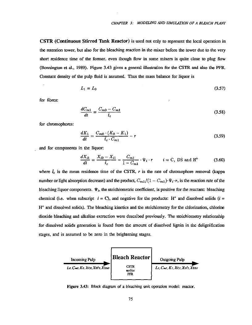
CHAPTER 3: MODELING AND SIMULATION OF A BLEACH PLANT
CSTR (Continuous Stirred Tank Reactor) is used not only to represent the local operation in
the retention tower, but also for the bleaching reaction in the mixer before the tower due to the very
short residence time of the former, even though flow in some mixers is quite close to plug flow
(Bennington et al., 1989). Figure 3.43 gives a general illustration for the CSTR and also the PFR.
Constant density of the pulp fluid is assumed. Thus the mass balance for liquor is
(3.57)Ll = LO
for fibres:
dCmi Cmo — Cmi dt
for chromophores:
Cmo • (Ko — _dt^t, • Cmi
and for components in the liquor:
dXii X0 — Xii^Cmidt^I^1 — Cnii^• r
(3.58)
(3.59)
i = C, DS and II+^(3.60)
where i is the mean residence time of the CSTR, r is the rate of chromophore removal (kappa
number or light absorption decrease) and the product, Cmi 1(1 — Cmi)•Ti.r, is the reaction rate of the
bleaching liquor components. W, the stoichiometric coefficient, is positive for the reactant: bleaching
chemical (i.e. when subscript i = C), and negative for the products: H+ and dissolved solids (i =
II+ and dissolved solids). The bleaching kinetics and the stoichiometry for the chlorination, chlorine
dioxide bleaching and alkaline extraction were described previously. The stoichiometry relationship
for dissolved solids generation is found from the amount of dissolved lignin in the delignification
stages, and is assumed to be zero in the brightening stages.
Incoming Pulp
Lo,Cmo,Ko,Xco,X1ro,XDso
Bleach ReactorCSTRand/orPFR
Outgoing Pulp ow
Li. Crn,, K , XCI, X11+1,XDSI
Figure 3.43: Block diagram of a bleaching unit operation model: reactor.
75
Chapter 3: MODELING AND SIMULATION OF A BLEACH PLANT
PFR (Plug Flow Reactor) is part of the model for the retention tower. If constant density of the
pulp fluid is assumed, the mass balance for liquor becomes
(3.61)
for fibres:
for chromophores:
ac„,^ac,„_at^at
OK OK= — —at^at
(3.62)
(3.63)
and for components in liquor:
OXi^OXi^Cm= — Ti • rOt^Ot^1C„,
i = C, DS and II+^(3.64)—
Equations 3.62 to 3.64 are two-dimensional partial differential equations with respect to the operating
time, t, and the residence time, i They cannot be directly solved by SIMNON. They are converted
as follows:'-y /\ = c7no (t — tp )
67 (t — ip) =^— ip)
K1(t) = K(t — tp)
K(t — tp) = Ko(t — tp) — Jr. dt^ (3.65)
X ii(t) = X(t — fp)
—
X(t — fp) = Xio(t — fp)^C„,o(t fp)
1 — C,,o(t — tp) Ti • r• dt
These equations mean that the output stream variables of the PFR,^Kj and X11 are delay functions
of the variables CO3 IC,:; and ,c1.0, respectively. i,, is the time delay and also the residence time of
the reactor. C7n0, K61` and X:0 at the time t - ip are the reactor outputs at the same time under the
steady-state operation but, under the dynamic operation, they are the outputs of ip later.
The time delay function is provided by the SIMNON's internal library while a Runge-Kutta-
Fehlberg algorithm, written as a FORTRAN subroutine, was added to SIMNON to solve the
integration in the I direction (i.e., along the flow path).
tp
76
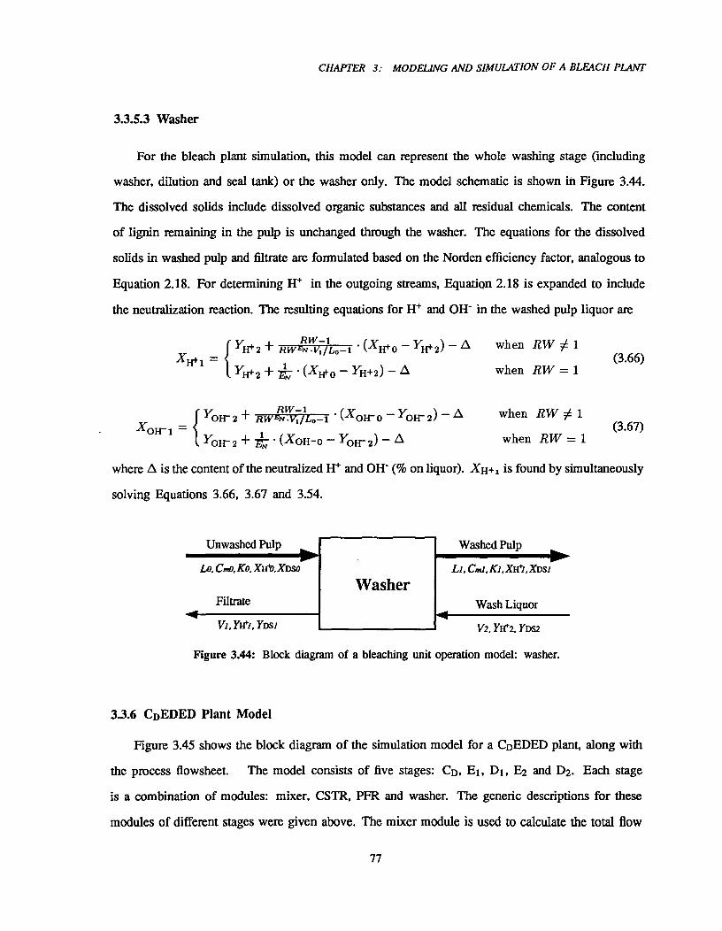
RW-1 YOH- 2 + RWEN •VaLo-1 (X0H- - YOH- 2) - A
XOlr 1 -when RW 1
(3.67)when RW = 1YoH-2 + k • (x0H-0 — YoH-2)— A
molUnwashed Pulp
-411^
Lo,Cmo, Ko, Kat, XDSO
Filtrate
V/ YH'/, YDS/
Washer
CHAPTER 3: MODELING AND SIMULATION OF A BLEACH PLANT
3.3.5.3 Washer
For the bleach plant simulation, this model can represent the whole washing stage (including
washer, dilution and seal tank) or the washer only. The model schematic is shown in Figure 3.44.
The dissolved solids include dissolved organic substances and all residual chemicals. The content
of lignin remaining in the pulp is unchanged through the washer. The equations for the dissolved
solids in washed pulp and filtrate are formulated based on the Norden efficiency factor, analogous to
Equation 2.18. For determining 11+ in the outgoing streams, Equation 2.18 is expanded to include
the neutralization reaction. The resulting equations for II+ and OH- in the washed pulp liquor are
XH+ ={ liff+ 2 + RWERNI:V1711-1L0-1 (XH+ 0 -111+2) - A
YHF 2 + 117," • (Xlie- 0 - YH+2) - A
when RW 1
when RW = 1(3.66)
where A is the content of the neutralized H+ and OH- (% on liquor). XH+1 is found by simultaneously
solving Equations 3.66, 3.67 and 3.54.
L Washed Pulp^op.
Li, Cna, Ki, MP, XDS/
Figure 3.44: Block diagram of a bleaching unit operation model: washer.
3.3.6 CDEDED Plant Model
Figure 3.45 shows the block diagram of the simulation model for a CDEDED plant, along with
the process flowsheet. The model consists of five stages: CD, El, D1, E2 and D2. Each stage
is a combination of modules: mixer, CSTR, PFR and washer. The generic descriptions for these
modules of different stages were given above. The mixer module is used to calculate the total flow
Wash Liquor
V2, YHF2, YDS2
77
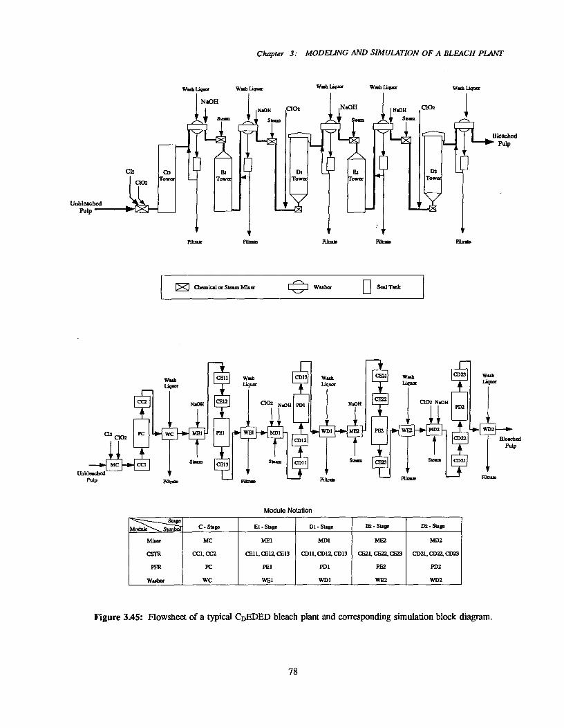
_T
FiltrateFiltrate Filtrate Mute^ Minor
^ Chemical or Steam Mixer Washer^Seal Tank
Wash Liquor
NaOHSeam
C102
Wash Liquor Wash Liquor Wash Liquor
Bleached• pulp
NaOHC102 NaOH
Steam
TowCo
TowerD2
TowerEa
TowerDl
TowerE2
Tower
CD23
PD2
-0-CD22
1
WashLiquor
WD21--110-
BleachedPulp
Alava
Wash CBI ILiquor
NaOH CEI2
Cl2 PC PEI-0- WC^MEI
SteamMC I c,E13
VPatrols
Unbleached -Pulp
Chapter 3: MODELING AND SIMULATION OF A BLEACH PLANT
Module Notation
StageModule^S^bol C - Stage El - Stage Di- Stage E2 - Stage 02 - Stage
Mixer
CSTH
PPR
Washer
MC
CC1, CC2
PC
WC
ME1
CE11, CE12, CE13
PEI
WEI
MD1
CD11, CD12, CD13
PD1
WD1
ME2
CE21, CE22, CE23
PE2
WM
MD2
CD21, CD22, CD23
P02
WD2
Figure 3.45: Flowsheet of a typical CDEDED bleach plant and corresponding simulation block diagram.
78
CHAPTER 3: MODELJNG AND SIMULATION OF A BLEACH PLANT
rate and initial chemical(s) composition of the bleaching reaction after the pulp slurry is mixed with
the chemical (02, NaOH and C102) and steam. A combination of CSTRS with a PFR is used to
estimate the state of pulp leaving the retention tower. The CSTRS+PFR structure is changeable in
the process simulator. Figure 3.45 shows a typical case. The bleaching reaction occurring in each
tower distinguishes it from the other towers. The bleaching kinetics involved in all the tower models
have been discussed in the section 3.3.3. The bleaching reaction occurring in the actual mixer is
lumped into the tower model. But the mixer reaction can be represented separately if necessary,
for example, by studying the sensor response after the mixer and local process control. The washer
module is used to determine the dissolved solids carryover of the pulp leaving each stage. Equation
3.48 was used to convert the kappa number leaving the El stage into the light absorption coefficient
entering the D1 stage.
The model was formulated along the pulp flow path through the plant and, therefore, does not
account for any recycled streams. Inclusion of recycle for dilution and washing could result in
changes in the dissolved solids content, pH values and temperatures which will in turn affect the
pulp bleaching reactions. The model assumes that the pulp liquors are neutral before mixing with
acidic or basic chemicals and that the dissolved solids in the pulp do not consume chemicals. Also,
the reaction temperatures are taken as input parameters since an energy balance is not included in
the model. However, these aspects can be incorporated into the simulation later according to the
needs of the particular problem to be studied. Bleaching kinetics, flow patterns and mass balances
along the pulp flow path are regarded as the essential features for modeling the dynamic behavior
of a multistage bleach plant and are already covered by the present model. The model can simulate
the dynamic responses of the kappa number after the delignification stages, brightness (from light
absorption coefficient) after the brightening stages, residual chemicals, final pH and dissolved solids
carryover for changes in chemical charges, unbleached kappa number, incoming dissolved solids
content and production rate.
The input variables include bleaching kinetic constants; temperature of bleaching reactions; mean
residence time of retention towers; parameters of the tower flow performance (CSTR number and
PFR fraction); liquor density; Norden efficiency factor and outlet consistency of washers; consistency,
79
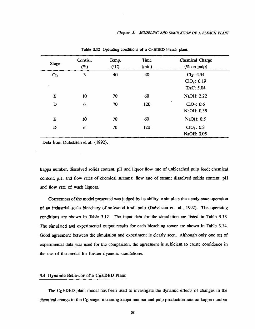
Chapter 3: MODELING AND SIMULATION OF A BLEACH PLANT
Table 3.12 Operating conditions of a CDEDED bleach plant.
StageConsist.
(%)Temp.(0c)
Time(min)
Chemical Charge(% on pulp)
CD 3 40 40 02: 4.54002: 0.19TAC: 5.04
10 70 60 NaOH: 2.22
D 6 70 120 002: 0.6NaOH: 0.35
E 10 70 60 NaOH: 0.5
6 70 120 002: 0.3NaOH: 0.05
Data from Dubelsten et al. (1992).
kappa number, dissolved solids content, pH and liquor flow rate of unbleached pulp feed; chemical
content, pH, and flow rates of chemical streams; flow rate of steam; dissolved solids content, pH
and flow rate of wash liquors.
Correctness of the model presented was judged by its ability to simulate the steady-state operation
of an industrial scale bleachery of softwood kraft pulp (Dubelsten et. al., 1992). The operating
conditions are shown in Table 3.12. The input data for the simulation are listed in Table 3.13.
The simulated and experimental output results for each bleaching tower are shown in Table 3.14.
Good agreement between the simulation and experiment is clearly seen. Although only one set of
experimental data was used for the comparison, the agreement is sufficient to create confidence in
the use of the model for further dynamic simulations.
3.4 Dynamic Behavior of a CDEDED Plant
The CDEDED plant model has been used to investigate the dynamic effects of changes in the
chemical charge in the CD stage, incoming kappa number and pulp production rate on kappa number
80
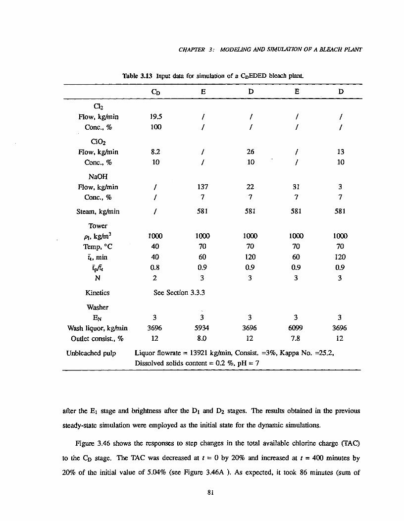
CHAPTER 3: MODELING AND SIMULATION OF A BLEACH PLANT
Table 3.13 Input data for simulation of a CDEDED bleach plant.
CD E D E D
C12Flow, kg/min
Conc., %
002
19.5100
Flow, kg/min 8.2 / 26 / 13Conc., % 10 / 10 / 10
NaOHFlow, kg/min / 137 22 31 3
Conc., % / 7 7 7 7
Steam, kg/min / 581 581 581 581
Towerp1, kg/m3 1000 1000 1000 1000 1000Temp, °C 40 70 70 70 70
4, min 40 60 120 60 120IA 0.8 0.9 0.9 0.9 0.9N 2 3 3 3 3
Kinetics See Section 3.3.3
WasherEN 3 3 3 3 3
Wash liquor, kg/min 3696 5934 3696 6099 3696Outlet consist., % 12 8.0 12 7.8 12
Unbleached pulp^Liquor flowrate = 13921 kg/min, Consist. =3%, Kappa No. =25.2,Dissolved solids content = 0.2 %, pH = 7
after the Ei stage and brightness after the Di and D2 stages. The results obtained in the previous
steady-state simulation were employed as the initial state for the dynamic simulations.
Figure 3.46 shows the responses to step changes in the total available chlorine charge (TAC)
to the CD stage. The TAC was decreased at t = 0 by 20% and increased at t = 400 minutes by
20% of the initial value of 5.04% (see Figure 3.46A). As expected, it took 86 minutes (sum of
81

Chapter 3: MODELING AND SIMULATION OF A BLEACH PL4iV7'
Table 3.14 Comparison between predicted and experimental dataat steady state after retention towers of a CDEDED bleach plant.
Stage
Chromophores
cal.^exp.
Residual chem.
(% on liquor)
pH
cal.^exp.
Dissolvedsolids
(% on liquor)CD kappa:12.6 C12: 3.25x 10⁻² 1.6 0.481
E kappa:5.6^5.3 NaOH: 5.81x 10⁻³ 11.2^11.0 0.628
D bright.:74.9^75.3 C102: 5.33x 10⁻³NaOH: 1.16x 10⁻¹°
3.5^3.7 0.169
E bright.:74.9 NaOH: 9.60x 10⁻² 12.4 8.93x 10⁻²
C102: 8.05x 10 -3D bright.:88.8^89.2NaOH: 3.44x 10⁴°
3.9^3.8 3.78x 10⁻²
Experimental data from Dubelsten et al. (1992).Operating conditions are listed in Table 3.12.
PFR residence times of the CD and El stages) and a short-time dynamic process for the CE kappa
number to respond to each input change (see Figure 3.46B ). The CED brightness and final brightness
responded more slowly and with lower magnitude than the CE kappa number (see Figures 3.46C
and 3.46D). It took about 230 minutes for the CED brightness to decrease from 74.9 to 68.5% ISO
and 410 minutes for the final brightness to decrease from 88.8 to 87.5% ISO after the 20% decrease
was made in the TAC. Due to the nonlinearity of bleaching kinetics, the response gain of each stage
for the decrease in the chemical charge was apparently different from that for the chemical charge
increase. The former is approximately double that of the latter in the simulated case. Step responses
of the bleach plant to ±20% changes in the incoming kappa number have also been simulated and
the results are similar to those shown in Figure 3.46.
Another dynamic simulation employed incoming kappa number fluctuations derived from on-line
measurements in Swedish mills (Edlund, Lundquist and Hansson, 1992). The simulated disturbances
duplicated the magnitudes and frequencies of the actual disturbances. Referring to Figure 3.47A, large
magnitude variations in the incoming kappa number over a period of 5000 minutes proceeded quite
slowly in comparison with the process dynamics. Consequently, they all passed through the system
82

CHAPTER 3: MODELING AND SIMULATION OF A BLEACH PLANT
6
riR5.5
5
c.5.5 4.5
4
(A)
7.9
7A6.9
6.4
e 5.9
5.4
4 .9
4.4
(B)
78
• 76
(C)
74
• 72
70
• 68
tsR89
88
87
.o86
(D)
0^200^400^600^800^1000
Time (min)
Figure 3.46: CDEDED bleach plant response to step changes in total available chlorine charge in CD stage.
83
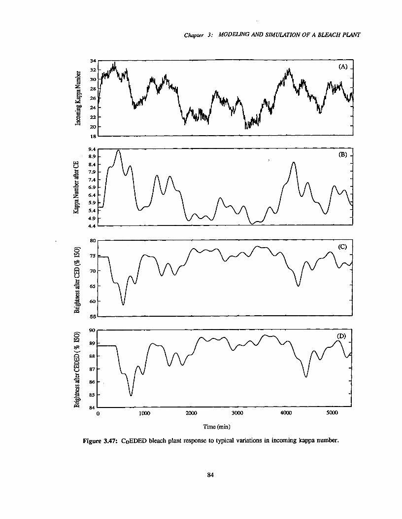
9.4
8.9
8.4
7.9
7.4
6.9
6.4
5.9
5.4
4.9
4.4
80
75
70
65
60
55
90
89
88
87
86
85
840 1000 5000400030002000
Chapter 3: MODELING AND SIMULATION OF A BLEACH PLAM'
(A) .._
_
-
-_
Time (min)
Figure 3.47: CDEDED bleach plant response to typical variations in incoming kappa number.
84
CHAPTER 3: MODELING AND SIMULATION OF A BLEACH PLANT
without control, resulting in the obvious changes in CE kappa number, CED and final brightness as
shown in Figures 3.47B, 3.47C and 3.47D. The CPU time taken for this simulation was 70 minutes.
Figure 3.48 shows the bleach plant responses when the pulp production rate was raised from 431
to 647 kg/min at t.-0 (i.e., a 15% step change). These responses were much more complex than those
for the changes in chemical charge and incoming kappa number. The response of the second stage
(E1) consisted of three distinct parts; the response in the third stage (D1), four parts and the response
in the fifth stage (D2), six parts. This was attributable to the fact that the change in production rate
caused changes in both the residence time and initial chemical concentration for all stages. The initial
response of each stage resulted from the decrease in its residence time. The residence time decrease
was gradual in the plug flow portion of the tower and produced a smaller time delay. The second
response was due to the reduction in the initial chemical concentration. It followed that the responses
to the changes in the previous stages (decrease in residence time and initial concentration) appear one
at a time. Again, insensitivity of the final stage to the input change was found. For a 15% increase
in production rate, the CE kappa number rose by 25% of its initial value after 110 minutes. The
CDED brightness decreased by 6% while the final brightness only dropped by 1%.
3.5 Conclusions
It was the objective of this work to develop a dynamic model of a multistage bleach plant.
Through an analysis of the process operations in a typical bleaching sequence, the tower flow pattern,
bleaching kinetics and relationship between the different chromophore indicators were identified as
fundamental aspects which needed detailed study.
From the tracer responses of typical bleaching towers, the pulp flow in the tower was found to
be a combination of agitated mixing and plug flow. Among all the models tested, a cascaded CSTR's
and PFR model was found to give the best representation of the experimental results. This model
is proved to be the most successful at characterizing the retention tower for the purpose of bleach
process control. The typical extent of mixing and fraction of plug flow in this model were also
obtained. The CSTRS+PFR and PFR models were compared with respect to their ability to predict
85
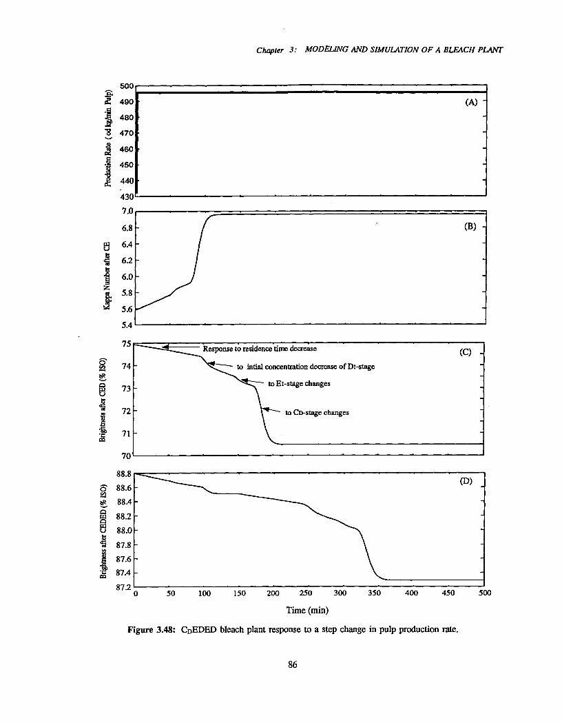
(A) -
■■1
■■1
(B) -
-
_
500IS;4 490
480
470
460
450
440
4307.0
6.8
6.4
6.2
6.0
5.8
5.6
.s
.......
A.....
1
Chapter 3: MODELING AND SIMULATION OF A BLEACH PLANT
5.4
Response to residence time decrease
to finial concentration decrease of Di-stage
.411---- to El-stage changes
(C) -
_--
to CD-stage changes
--_
75
cob- 74a*
70
88.888.688.488.288.0
87.887.687.4
87.2 0 50050^100^150^200^250^300
^350^
400^
450
Time (min)
Figure 3.48: CDEDED bleach plant response to a step change in pulp production rate.
86
CHAPTER 3: MODELING AND SIMULATION OF A BLEACH PLANT
the reaction responses of the chlorine tower and the first chlorine dioxide tower. The CSTRS+PFR
model was able to more realistically represent transient responses in kappa number, brightness and
residual chemicals than the PFR model when the chemicals charge or incoming kappa number was
changed. The former can not only describe long-time delay but also low-order dynamic response of
the tower. The choice between the CSTRS+PFR and PFR models did not seem to significantly affect
the calculations of the steady-state bleaching results.
So far, kinetic studies have been conducted for chlorine delignification, alkaline extraction and
chlorine dioxide bleaching of kraft pulp. From the published kinetic models, those considered to
be reliable and suitable for process simulation were incorporated in this work. The model for the
first extraction was modified and the new model gave a better prediction for the effects of changing
chlorine or chlorine dioxide charge.
A theoretical analysis showed that the light absorption coefficient may be linearly related to the
kappa number for a delignified pulp. The linear correlation between the light absorption coefficient
and the kappa number after the El stage was determined using experimental data. It allows the
connection of the delignification and succeeding brightening phase, and thus makes possible the
simulation of the whole bleach plant.
The dynamic model of the CDEDED bleach plant was assembled by linking the unit operation
models for mixing, reaction and washing. The model was validated by checking the steady-state
simulation against available experimental results.
The applicability of the CDEDED bleach plant model was illustrated by following the dynamic
behavior of the system due to changes in chlorine charge, incoming kappa number and production
rate. The responses of CE kappa number as well as CED and final brightness to step changes in the
chemical charge had strong nonlinearity and a long time delay. The responses of later stages were
less sensitive than those of the earlier stages. When the production rate was changed, the system
demonstrated complicated interactions.
In conclusion, this study has established a base for further work in the process simulation
and control of multistage bleach plants by use of the dynamic simulation package, SIMNON. The
87

Chapter 3: MODELING AND SIMULATION OF A BLEACH PLANT
simulator developed has been successfully used in predicting both the steady-state and dynamic
behaviors of the a CDEDED bleaching sequence. For modelling other types of sequences where
different bleaching agents are used, more information on bleaching kinetics is necessary; but the
methodologies developed for describing the tower flow pattern, connection of the delignification with
brightening phases and the unit operations should be directly adaptable.
3.6 Recommendations and Suggestions for Future Work
The major recommendation for future work is to develop dynamic simulators for commercial
bleach plants on the basis of the present work and apply them to improve process control strategies.
This general recommendation gives rise to the following specific suggestions.
1. To study and model chemical kinetics of modern bleaching technologies such as delignification
with high chlorine dioxide substitution, alkaline extraction with addition of oxygen, etc. ThisN...
is the most essential step towards simulating a commercial bleaching sequence.
2. To account for the heat effects due to dilution, heating, washing and chemical reaction.
3. To study the buffering capacities of different components in bleaching liquor in order to
provide an accurate estimates of pH.
4. To incorporate recycle schemes into the simulation.
5. To test the predictions of the developed models against mill measurements.
6. To apply the dynamic simulator to process control practices.
88
CHAPTER 4: GENERAL CONCLUSIONS
CHAPTER 4
GENERAL CONCLUSIONS
In this study, dynamic process simulators for brown stock washing plants and multistage bleach
plants have been developed and preliminarily validated. SIMNON software has been used as the
main tool to construct computer models and perform simulations. The simulator of the brown stock
washing system provides a simple but accurate method to quantify the interactions among the process
components and to predict system dynamic response to changes in major process variables. The model
has been used to investigate the dynamic behavior and evaluate the process control strategies for a
three-stage countercurrent washing plant. The simulator of the bleach plant gives realistic descriptions
for the dynamic characteristics of the process such as long-time delays and strong nonlinearity. It
can be used not only to simulate a CDEDED plant but also other types of bleach plants as long as
the bleaching kinetics used in these sequences are available. Connection of these two simulators will
constitute simulation for a process from the brown stock after digestion through to the final bleached
product. This is significant for understanding the dynamics of an entire kraft pulping process and
thus designing better control systems.
Through the course of this study, it becomes obvious that a successful dynamic process simulator
can only be constructed on the basis of accurate mathematical models, a sufficient data base and
powerful computer technology. There is still much work that needs to be done in these three areas
to develop useful models of the complex processes in the pulp industry.
89
REFERENCES
Ackert, J. E., "Kraft Pulp Chlorination Kinetics", Ph.D. Thesis, University of Idaho, Moscow
(1973).
Ackert, J. E., D. D. Koch, and L. L Edwards, "Displacement Chlorination of Kraft Pulps —
An Experimental Study and Comparison of Models", TAPPI J. 58(10), 141 (1975).
AxegArd, P., "Kinetics of Alkaline Bleaching for the Kraft CE Sequence", Svensk Papperstiding
81(12), 361-367 (1979).
AxegArd, P., U. Jansson, and A Teder, "The E2 Stage Improves the Reactivity of Pulp Towards
Chlorine Dioxide", J. Pulp Paper Sci. 10(1), 1-5 (1984).
AxegArd, P., S. Moldenius, and L. Olin, "Basic Chemical Kinetic Equations are Useful for an
Understanding of Pulping Processes", Svensk Papperstiding 81(5), 131-136 (1979).
Bennington, C. P. J., R. J. Kerekes, and J. R. Grace, "Mixing in Pulp Bleaching", J. Pulp
Paper Sci. 15(5), 186-195 (1989).
Biallcowski, W. L., "Bleach Plant Process Control", in "1990 Bleach Plant Operations", TAPPI
Seminar Notes (1990), pp. 189.
Bonar, L., and J. D. Munro, "Improvements in C12 Mixing at Crofton", in Prodeedings of
CPPA Spring Conference (1979), pp. 136-140.
Branch, C. A., and S. Muller, "Physical Properties of Kraft Pulp Black Liquor", Appita 44(5),
339-341 (1991).
Brenner, H., "The Diffusion Model of Longitudinal Mixing in the Beds of Finite Length,
Numerical Values", Chem. Eng. Sci. 17, 229-236 (1962).
Brownell, L. E., and D. L. Katz, Chem. Eng. Progr. 43(11), 602 (1947).
Carman, P. C., "Flow of Gases Through Porous Media", Academic Press., New York (1956).
Chapnerka, V. D., "A Kinetic Study of the Chlorination of Unbleached Kraft Pulp", Ph.D.
Thesis, University of Florida (1961).
90

Cholette, A., and L. Cloutier, "Mixing Efficiency Determination for Continuous Flow Systems",
Can. J. Chem. Eng. 37, 105-112 (1959).
Crotogino, R. H., N. A. Poirier, and D. T. Trinh, "The Principles of Pulp Washing", TAPPI
J. 70(6), 95-103 (1987).
Crotogino, R. H., D. T. Trinh, N. A. Poirier, and D. T. Wearing, "Pulp Washing' 83 — A
Review", in Proc. of International Chemical Reconvery (TApPI) (1985).
Darcy, H., "Les Fontaines Publiques de La Ville de Dijon", Victor Dalmint, Paris (1856).
Dubelsten, P., S. G. Arinobu, and C. J. Kanters, "The Compatibility of C/D with Oxidative
Extraction", Pulp Paper Can. 93(4), 24-27 (1992).
Edlund, S. G., S.-0. Lundquist, and A. Hansson, "Experiences from the STFI OPTI-Kappa
and its Use for the Control of Pulping Processes", Pulp Paper Can. 93(12), 118-122 (1992).
Edwards, L. L., R. Baldus, and R. Abbot, "GEMS Documentation Describing Data Input,
Simulation Control and Simulation Options", University of Idaho, Chemical Engineering
Department (1983).
Edwards, L. L., G. Hovsenius, and H. Norrstrtim, "Bleaching Kinetics: A General Model",
Svensk Papperstidning 76(3), 123-126 (1973).
Edwards, L. L., Peyron M., and Minton M., "Models for Cross-flow Pulp Washing
Calculations", Pulp Paper Can. 87(1), 67 (1986).
Forgacs, 0. L., A. A. Robertson, and S. G. Mason, "The Hydrodynamic Behavior of Paper-
Making Fibres", Pulp Paper Mag. Canada 59(5), 117 (1958).
Germgard, U., "Stoichiometry of Chlorine Dioxide Prebleaching of Softwood Kraft Pulp",
Svensk Papperstiding 85(6), R43-50 (1982a).
Genngird, U., "Stoichiometry of Prebleaching of Softwood Kraft Pulp with Chlorine Dioxide
and Small Fractions of Chlorine", Cellulose Chem. Technol. 48(17), 35-48 (1982b).
GermgArd, U., and R.-M. Karlsson, "Kinetics and Stoichiomentry of CE-Prebleaching of
Softwood Kraft Pulp", Svensk Papperstiding 88(85), R146-150 (1985).
91
GermgArd, U., and H. Lindberg, "A Mathematical Model for (D+C)-Prebleaching", Svensk
Papperstiding 85(18), R172-176 (1982).
GermgArd, U., and B. SjOgren, "Ozone Prebleaching of Modified-Cook and Oxygen-Bleached
Softwood Kraft Pulp", Svensk Papperstiding 88(15), R127-132 (1985).
GermgArd, U., and A. Teder, "Kinetics of Chlorine Dioxide Prebleaching", Trans. Tech. Sect.
CPPA 5(6), 31-36 (1980).
GermgArd, U., A. Teder, and D. Tormund, "The Relative Rates of Consumption of Chlorine and
Chlorine Dioxide During (D+C) Bleaching Softwood Kraft Pulp", TAPPI J. 65(5), 124-126
(1982).
GermgArd, U., A. Teder, and D. Torrnund, "Mathematical Models for Simulation and Control
of Bleaching Stage", Nordic Pulp Paper Res. 2(1), 16-22 (1987).
Han, S. T., and W. L. Ingmason, "A Simplified Theory of Filtration", TAPPI J. 50(4), 176
(1967).
Han, Y., "Flow through Porous Media: Impact of Flow on Wood Pulp Washer Performance",
Master's Thesis, University of Idaho, Moscow (1985).
Han, Y., "Modelling and Simulation of Wood Pulp Washers", Ph.D. Thesis, University of
Idaho, Moscow (August 1989).
Hisey, R. W., "An Investigation of the Mechanism of the Dewatering of Compressible Beds",
TAPPI J. 39(10), 690 (1956).
Histed, J. A., and C. R. Vega, "Optimum Chlorination Stage Conditions", Pulp Paper Can.
88(1), T22-25 (1987).
Hsu, C., and J. S. Hsieh, "Reaction Kinetics in Oxygen Bleaching", AIChE J. 34(11), 116-122
(1988).
Ingmason, W. L., and B. D. Andrews, "High-Velocity Water Flow Through Fibre Mats",
TAPPI J. 35(3), 150-155 (1963).
Karter, E. M., "The Role of Physico-Chemical Rate Phenomena in Wood Pulp Chlorination",
Ph.D. Thesis, University of Maine, Orono (1968).
92
Kerekes, R. J., R. M. Soszynsky, and P. A. Tam Doo, "The Flocculation of Pulp Fibres",
in Transactions of the Eight Fundamental Research Symposium, Oxford, vol. 1 (1985), pp.
265-310.
Korhonen, 0., "Brownstock Washing: A Review of Current Technology", Pulp Paper J. (9),
104 (1979).
Kovasin, K., H. V. Norden, and L. Ahonen, "Modelling the Filtration Stage of a Pulp Washer",
Filtration & Separation 25(1), 42 (1988).
Kubellca, P., and F. Munk, Z. Tech. Physik 12, 593 (1931).
Kuo, M. T., "Filtrate Cake Washing Performance", AIChE J. 6(4), 566 (1960).
Lee, P. F., "Optimizing the Displacement Washing of Pads of Wood Pulp Fibres", TAPPI
62(9), 75-78 (1979).
Levenspiel, 0., "Chemical Reaction Engineering", John Wiley & Sons Inc., New York, 2nd
Ed (1972).
Liebergott, N., "General Principles of Pulp Bleaching", PAPRICAN Course Notes (1991).
Lundquist, S.-0., "Pulp Washing Control: Principle and Results", Pulp Paper Can. 86(11),
72-76 (1985).
Lundquist, S.-0., and H. Nordstrom, "The Development of a Control System for a Pulp
Washing Plant Through the Use of Dynamic Simulation", in 1FAC./PRP 4 Automation
Symposium Proc., Belgium (June 1980), pp. 3-5.
Luthi, 0., "Different Approaches to Model Displacement Ratios", in Proc. of Pulp Washing
Symposium (Tech Sect., CPPA), Quebec (September 1983), pp. 9.
Luthi, 0., "Mechanics of Thick Mats", in Pulp Washing Symposium Proc., Marihamn, Finland
(May 1987), pp. 1987.
Mackinnon, J., "Dynamic Simulation of the First Two Stages of a Kraft Softwood Bleach
Process", Master's Thesis, McGill University (1987).
MAPPS, "MAPPS User's Guide", The Institute of Paper Chemistry, Appleton, WI (1984).
93
MASSBAL, "MASSBAL MKII System Documentation", SACDA, University of Western
Ontario (1983).
McConnell, R. R., 0. Syberg, and N. W. Wild, "Introduction to Process Simulation", TAPPI
Press, 2nd Ed (1992).
Moller, K., G. G Duffy, and A. L. Titchener, "The Laminar Plug Flow Regime of Paper Pulp
Suspensions in Pipes", Svensk Papperstidning 74,829 (1971).
Moreira, R. M., and R. M. Felder, "Residence Time Distributions of Paper Pulp Slurries in
Vertical Laminar Flow", AIChE J. 25(1), 131-143 (1979).
Myers, M. R., and L. L Edwards, "Development and Verification of Predictive Oxygen
Delignification Model for Hardwood and Softwood Kraft Pulp", TAPPI J. 72(9), 215-219
(1989).
NNse, T., and K.-E. Sjoberg, "Advanced Control of a Drum Washing Plant", Pulp Paper Can.
90(9), 108-111 (1989).
Norden, H. V., "Analysis of a Pulp Washing Filter", Kemian Te,ollisuus 23(4), 344-351 (1966).
Norden, H. V., "Statistical Analysis of Pulp Washer on an Industrial Rotary Drum", Pulp
Paper Mag. Can. 74(10), 83-90 (1973).
Norden, H. V., and M. Peldcanen, "General Calculation Method for Stagewise Models of Pulp
Washing and Other Mass and Heat Transfer", in Pulp Washing'87 Symposium (CPPA Trans.
Techn. Sect.) (September 1987), pp. 237.
NorrstrOm, H., "Light Absorption of Pulp and Pulp Components", Svensk Papperstiding 75(22),
891-899 (1972).
Olin, L., and A. Teder, "The Kinetics of Oxygen Bleaching", TAPPI J. 62(43-50), 12 (1979).
PAPDYN, "PAPDYN Process Simulation Package", Pulp and Paper Research Institute of
Canada (1991).
PAPMOD, "PAPMOD Process Simulation Package", Pulp and Paper Research Institute of
Canada (1988).
94
Paterson, A. H. J., and R. J. Kerekes, "Fundamentals of Mixing in Pulp Suspensions:
Measurement of Microscal Mixing of Chlorine", J. Pulp Paper Sci. 11(4), 108-113 (1985).
Paterson, A. H. J., and R. J. Kerekes, "Fundamentals of Mixing in Pulp Suspensions:
Measurement of Microscal Mixing in Mill Chlorination Mixers", J. Pulp Paper Sci. 12(3),
J78–J83 (1986).
Pattyson, G., "Kamyr MC Mixer for Chlorine Dioxide Mixing at Great Lakes Forest Products,
Thunder Bay, Ontario", in Proc. of the 70th Annual CPPA Meeting, Monteal (1984), pp.
A63–A68.
Pellet, G., "Longitudinal Dispersion, Intrapartical Diffusion and Liquid-Phase Mass Transfer
During Flow Through Multiparticle System", TAPPI J. 49(2), 75-82 (1966).
Perkins, J. K., "Channeling in Continuous Bleaching Cells (Pulp Behavior Patterns in Bleach
Towers)", in Prodeedings of TAPPI 25th Alkaline Pulping Conference (1971), pp. 191-198.
Perkins, J. K., "Mixers, Pumps and Towers — Design and Performance", in "Bleaching Plant
Operations", TAPPI Seminar Notes (1985), pp. 127-134.
Perkins, J. K., H. S. Welsh, and J. H. Mappus, "Brown Stock Washing Efficiency", TAPPI J.
37(3), 83-89 (1954).
Perron, M., and B. Lebeau, "A Mathematical Model of Pulp Washing on Rotary Drums",
Transactions of the Techn. Sect., CPPA 3(1), TR1–'TR5 (1977).
Perry, J. F., M. Gottlieb, and R. A. Hohn, "Dynamic Simulation of a Brown Stock Washer",
in ISA/75 Pulp and Paper Division Symposium Proc., Milwaukee, Wisconsin (1975), pp.
45-56.
Poirier, N. A., R. H. Crotogino, and W. J. M. Douglas, "Displacement Washer of Wood Pulp
— A Model with Source Term for Low Initial Liquor Concentration", in Pulp Washing '87
Symposium (CPPA/TS), Mariehamn, Finland (1987a).
Poirier, N. A., R. H. Crotogino, and W. J. M. Douglas, "Displacement Washer of Wood Pulp
— A Model with Source Term for Higher Initial Liquor Concentration", in Pulp Washing
'87 Symposium (CPPA/TS), Mariehamn, Finland (1987b).
95
Poirier, N. A., R H. Crotogino, D. T. Trinh, and W. J. M. Douglas, "Displacement Washer
of Wood Pulp — An Experimental Study at Low Initial Liquor Concentration", in Pulp
Washing '87 Symposium (CPPA/TS), Mariehamn, Finland (1987c).
Rapson, W. H., "TAPPI Monograph Series", TAPPI, 27 (1963).
Reynolds, E., J. D. Gibbon, and S. Attowood, "Smoothing Quality Variations in Storage Chests
Holding Paper Stock", Trans. Instn. Chem. Engrs 42, T13-T21 (1964).
Roada, R. H., "FlowCalc: A Flowsheet Calculation Program for Microcomputers", Simulation
Software, Custer, WI (1983).
Roche, A., and D. Bouchard, "Process Simulation in the Pulp and Paper Industry", Technical
Report M22, Pulp and Paper Research Institute of Canada (1982).
Russel, N. A., "A Study of the Initial Phase of the Aqueous Chlorination of Kraft Pulp Mills",
Ph.D. Thesis, Institute of Paper Chemisty, Lawrence College, Appleton (1966).
Sherman, W. R., "The Movement of a Soluble Material During the Washing of a Bed of
Packed Solids", AIChE J. 64(10), 855-860 (1964).
SIMNON, "SIMNON User's Guide for Unix System", Lund Institute of Technology, Sweden
(1991).
Sinn, S., "State-of-the-Art Chlorine Dioxide Mixer Installed at Weyerhaeuser", Pulp Paper
Can. 58(6), 119-121 (1984).
Snyder, J., "Measuring Bleaching Tower Retention Times", TAPPI J. 49(12), 105-106 (1966).
Sperry, D. R., "Deduction of Filtration Equation Including Term for Cloth Resistance and
Experiments to Verify Same", Chem. Met. Eng. 15, 198 (1916).
Taylor, R. A., Vega C. R., and J. A. Histed, "Numerical Simulation of the Extraction Stage
Stoichiometry and Rate", in Int'l Pulp Bleach Conf. (CPPA/TAPPI), San Diego (1982), pp.
107-113.
Teder, A., and D. Tormund, "Kinetics of Chlorine Dioxide Bleaching", Trans. Tech. Sect.
CPPA 3(2), 41-46 (1977).
96
Teder, A., and D. Tormund, "Mathematical Model for Chlorine Dioxide Bleaching and its
Applications", AIChE Symp. Ser. 76(200), 133-142 (1980).
Terry, N. A., and Wm. J. Frederick, "Kraft Recovery Boiler Physical and Chemical Processes",
American Paper Institute (1988), Ch. 2, pp. 62-64.
Tomiak, A., "Purging Calculations for Cascades of Mixing Stages", Can. J. Chem. Eng. 52(8),
502 (1974).
Torregrossa, L. 0., "Effect of Mixing on Chlorine Dioxide Bleaching", in TAPPI Pulping
Conference, Houston, TX (1983), pp. 635-641.
Trinh, D. T., N. A. Poirier, and R. H. Crotogino, "Displacement Washer of Wood Pulp — An
Experimental Study at High Initial Liquor Concentration", in Pulp Washing '87 Symposium
(CPPA/TS), Mariehamn, Finland (1987).
Turner, P. A., B. J. Allison, and J. K. Oei, "Brown Stock Washer Control (Part II: Filtrate Tank
Level Control)", in CPPA Annual Meeting Proc. (Book B), Techn. Sect., Quebec (December
1991), pp. 109-113.
Turner, P. A., A. A. Roche, J. D. McDonald, and A. R. P. Van Heiningen, "Dynamic Behavior
of a Brown Stock Washing Plant", in CPPA Spring Conference of Pacific Coast and West
Branches (CPPA, Techn. Sect.) (May 1991).
Ulinder, J. D., "Fixed Time Zone Methodology for Plug Flow Simulation as Applied to an
Oxygen Delignification Reactor", in Proc. of Control Systems' 92, Wistler (1992), pp. 181.
Venkatesh, V., and X. N. Nguyen, "Chemical Recovery in the Alkaline Pulp Processes",
TAPPI Press. (1985), Ch. 3, pp. 17-18.
Walker, 0. J., and A. Cholette, "Determination of the Optimum Size and Efficiency of Stock
Chests I. The Ideal Chest", Pulp Paper Mag. Can. 59,113-117 (1958).
Wigsten, A. L., "Conductivity—Based Shower Water Control In Brown Stock Washing", in
TAPPI Pulping Conf. Proc. (Book 1), New Orleans (November 1988), pp. 1-13.
Woodard, E. R., "A New Sensor for Brown Stock Washer Control", in TAPPI Pulping Conf.
Proc. (Book 1), New Orleans (November 1988), pp. 15-17.
97
APPENDIX: A: LITERATURE REVIEW OF PULP WASHING
APPENDIX A LITERATURE REVIEW OF PULP WASHING
Pulp washing has been traditionally described by two distinct approaches. One, called mecha-
nistic model here, is based on the knowledge of fundamental physical phenomena which control the
washing performance, such as filtration, two-phase flow, and displacement washing. The other, called
efficiency model, is based on a efficiency concept that lumps various phenomena together. A literature
review of the fundamental washing studies and washing efficiency concepts is presented below.
A.1 Fundamental Washing Studies
A.1.1 Filtration
The wood pulp fibres themselves are a porous media although the fluid within these pores is
not likely to flow. When the mat is formed during filtration, the filtrate is driven through the mat
by the pressure difference across the mat. Darcy's law (Darcy, 1856) can be used for liquid flow
through a porous media. On the basis of Darcy's law, Sperry (1916) suggested a model for filtration
in a cake which is growing in thickness, and has been proven useful in many applications. Many
who followed Sperry's model were mainly with finding a correlation for the resistance term in the
model for various filtration media. The resistance of a wood fibre mat depends on the compressible
nature of the fibre since the fibres form highly compressible mats during filtration. Comprehensive
research into the filtration and compression of wood pulp fibres has been carried out by 1ngmanson
and coworkers (Hisey, 1956; 1ngmason and Andrews, 1963; Han and 1ngmason, 1967) but also by
others (Han, 1985; Kovasin, 1988; Luthi, 1987).
A.1.2 Two-phase Flow
Two-phase flow occurs in the partially saturated fibre mat during dewatering, through which
liquid and air flow simultaneously. Darcy's law has been extended to the two fluid phases by
correlating the permeability of each phase to the saturation of the mat. The saturation is the ratio of
interfibre void volume occupied by the liquid to the total void volume of the mat. Calculation of the
permeability for the two-phase flow has been studied by a few authors (Brownell and Katz, 1947;
98
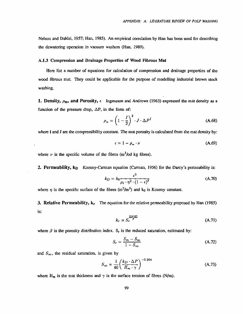
1 — SooSoo
Sr = — (A.72)
APPENDIX: A: LITERATURE REVIEW OF PULP WASHING
Nelson and Dahlsi, 1957; Han, 1985). An empirical correlation by Han has been used for describing
the dewatering operation in vacuum washers (Han, 1989).
A.1.3 Compression and Drainage Properties of Wood Fibrous Mat
Here list a number of equations for calculation of compression and drainage properties of the
wood fibrous mat. They could be applicable for the purpose of modelling industrial brown stock
washing.
1. Density, pm, and Porosity, E Ingmason and Andrews (1963) expressed the mat density as a
function of the pressure drop, AP, in the form of:
= (1 — 2 J • API^ (A.68)2
where I and J are the compressibility constant. The mat porosity is calculated from the mat density by:
c = 1 — p„, • v^ (A.69)
where v is the specific volume of the fibres (m3/od kg fibres).
2. Permeability, kD Kozeny-Carman equation (Carman, 1956) for the Darcy's permeability is:
= ko772 (1 —
where ri is the specific surface of the fibres (rn21m3) and ko is Kozeny constant.
E3(A.70)
3. Relative Permeability, kr The equation for the relative permeability proposed by Han (1985)
is:2-0_211,
I. _Qr $
where p is the porosity distribution index. Sr is the reduced saturation, estimated by:
(A.71)
and Soo, the residual saturation, is given by
= 1 (kij • APSoo 4Ok Hm, • 7
) -0.264
(A.73)
where Hm is the mat thickness and -y is the surface tension of fibres (N/m).
99
APPENDIX: A: LITERATURE REVIEW OF PULP WASHING
A.1.4 Displacement Washing
Displacement washing is the extraction of liquor in the mat by a piston effect with wash liquor
containing less solutes. Ideal displacement happens when no solute transfers between the wash
liquor and the original liquor in the mat. However, mixing and diffusion are unavoidable in actual
displacement washing. In addition, there is an adsorption/desorption equilibrium of the solute on fibre
surface if any solute is adsorbable. Brenner (1962) suggested an axially dispersed plug flow model
to represent non-ideal displacement using a single parameter, ie. Peclect number. This model was
extended by addition of a source term to account for adsorption (Sherman, 1964) and for intrafibre
diffusion (Pellet, 1966). Poirier and his coworkers (1987a; 1987b; 1987c) modelled displacement
washing of pulp for both high and low initial mat liquor concentration. They found that the axial
dispersion model without the source term was adequate for high solute concentrations, but inclusion
of a sorption isotherm was needed at low solute concentrations. Several studies (Pellet, 1966; Lee,
1979; Poirier et al., 1987c; Trinh et al., 1987) are available on the Peelet number of pulp fibre mats.
Displacement washing has also been modelled by Kuo (1960) and Han and Ingmason (1967) in a
quite different way from the dispersion model. The basic assumption of their model is that the mat
has been dewatered to its residual saturation such that the wash liquor passes through the empty
channels in plug flow and washing is primarily achieved by diffusion. But this assumption does not
fit pulp washing. Only a small portion of the mat liquor can be removed prior to washing in any
existing pulp washing equipment.
A.2 Washing Efficiencies
There are many methods of evaluating the efficiency of removal of dissolved solids from pulp
by various pulp washing systems. Displacement ratio factor and Norden efficiency are two of them
useful for simulation of industrial washing processes (Crotogino et al., 1985).
Displacement ratio, originating from Perkins (1954) is defined as the ratio of actual reduction
of dissolved solids to the maximum possible reduction. For most types of washing configurations
including the vacuum drum washer, displacement ratio is a strong function of the quantity of wash
100
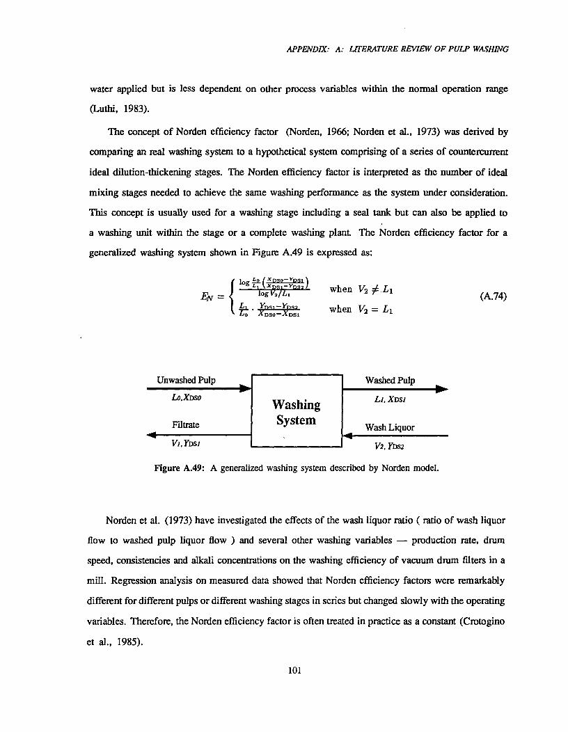
APPENDIX: A: LITERATURE REVIEW OF PULP WASHING
water applied but is less dependent on other process variables within the normal operation range
(Luthi, 1983).
The concept of Norden efficiency factor (Norden, 1966; Norden et al., 1973) was derived by
comparing an real washing system to a hypothetical system comprising of a series of countercurrent
ideal dilution-thickening stages. The Norden efficiency factor is interpreted as the number of ideal
mixing stages needed to achieve the same washing performance as the system under consideration.
This concept is usually used for a washing stage including a seal tank but can also be applied to
a washing unit within the stage or a complete washing plant. The Norden efficiency factor for a
generalized washing system shown in Figure A.49 is expressed as:
logjxrg:;:1^Z:3 EN =^togV21 Li
Ync,—Y11S2 Lo XDSO -XDS1
when V2 0 L 1
when V2 = L1(A.74)
Unwashed Pulp Washed PulpLo,XDSO
Filtrate
WashingSystem
XDSI
Wash LiquorV I ,YDS1 V2, YDS2
Figure A.49: A generalized washing system described by Norden model.
Norden et al. (1973) have investigated the effects of the wash liquor ratio ( ratio of wash liquor
flow to washed pulp liquor flow ) and several other washing variables — production rate, drum
speed, consistencies and alkali concentrations on the washing efficiency of vacuum drum filters in a
mill. Regression analysis on measured data showed that Norden efficiency factors were remarkably
different for different pulps or different washing stages in series but changed slowly with the operating
variables. Therefore, the Norden efficiency factor is often treated in practice as a constant (Crotogino
et al., 1985).
101
APPENDIX: A: LITERATURE REVIEW OF PULP WASHING
Washing efficiency is a steady state concept, representing the long-term performance of an actual
washing system. Thus, for modeling of dynamic behavior of a washing plant, the efficiency concept
can only be used to describe the washing component which has a negligible transient period compared
to the slow process component. The Norden efficiency factor has been used for the vacuum drum filter
in dynamic-simulations of brown stock washing systems (Lundquist, 1980; Nase and Sjoberg, 1989).
102
APPENDIX: B: LITERATURE REVIEW OF PULP BLEACHING
APPENDIX B LITERATURE REVIEW OF PULP BLEACHING
B.1 Lignin and Chromophores of Wood Pulp
Pure cellulose is white and does not contribute to pulp color. It is the chromophores contained
in the pulp which are responsible for absorbing light and thus for the color of pulp. Cluomophores
are coloured compounds, which absorb radiation in the ultra-violet and visible regions. The colour-
producing species of pulp are mainly lignin or lignin breakdown products. Lignin is a highly branch,
aromatic, three-dimensional polymer. In the lignin molecule, there are chemical groups containing
chromogenic structures (eg. carbonyl groups and double bonds). Chromogens form chromophoric
systems when they are present in suitable combination with benzene rings and auxomochromes (eg.
OH, OMe, Cl). The lignin in wood contains a number of coloured constituents. However, some of
lignin chromophoric groups result from reactions occurring during pulping and bleaching treatments.
The carbohydrates and extractives in pulp also contain chromophoric groups but contribute much less
to light absorption of pulp compared to lignin.
Bleaching of lignin in a lcraft pulp is achieved by lignin removal followed by lignin decolour-
ization which allows production of the desired brightness with minimal loss in pulp strength. The
principle of dilignification is to convert the remaining lignin into soluble fragments by chemical treat-
ment. For instance, lignin during chlorination reacts with chlorine to form chloro-lignins which are
partly water-soluble in the washing step and readily alkali-soluble in the next extraction stage. Pulp in
the delignification phase is characterized by its lignin content. The lignin content is usually measured
by the kappa number in bleaching physical chemistry as well as in the industry. The kappa number
is defined as the number of cubic centimeters of 0.1N potassium permanganate solution consumed
by 1 gram of moisture-free pulp. It relates linearly to the lignin content for all types and grades of
pulps up to yields of 70%. The content of lignin for unbleached softwood pulp is approximately
0.13 to 0.15 times the kappa number. For bleached pulp, the relationship between lignin and kappa
number is also a function of the extent of delignification and oxidation of the pulp since the kappa
number is determined by the reduction of potassium permanganate.
103
APPENDIX: B: LITERATURE REVIEW OF PULP BLEACHING
The decolourizing or brightening of pulp is concerned with selective elimination of chromophoric
groups in lignin without lignin removal by using an oxidizing agent or a reducing agent. Chlorine
dioxide is a conventional oxidant for bleaching kraft pulp. Pulp in this brightening phase is
characterized by its chromophore content. The overall content of the chromophores is expressed
in terms of brightness or by the light absorption coefficient of pulp. The brightness is a standardized
method of measuring the reflectance of a pulp sheet using blue light at a wavelength of 457nm. It
not only depends on the content of the light-absorbing components in pulp but also on the physical
structure of the pulp sheet. In contrast, the light absorption coefficient at 457m wavelength, in
the Kubelka-Munk equation (Kubelka and Munk, 1931; Rapson, 1963), is theoretically directly
proportional to the absorptivity of the material and thus to the chromophore content (NorrstrOm,
1972). Therefore, the light absorption coefficient is preferable for studying the kinetics of pulp
brightening reactions while the brightness is usually used as a technical unit to report the product
quality. Assuming a light scattering coefficient of the standard pulp brightness sheet, the light
absorption coefficient of the bleached pulp can be converted to the brightness using the Kubelka-
Munk equation.
B.2 Bleaching Kinetics of Kraft Pulp
B.2.1 Experimental Methods
Two principal methods have been used for obtaining experimental data and studying a bleaching
reaction from the kinetic point of view.
The first is the constant condition method, in which concentrations of active chemicals in
bleaching solution are held constant throughout the bleaching. This method has many advantages, eg.
O Simple mathematical treatment of the data.
O No assumption concerning the stoichiometry has to be made.
O Stoichiometry data are obtained if the liquor reactants are added continuously at the same
rate as they are consumed and the added amounts are measured.
O It is easy to separate different effects from each other.
104
APPENDIX: B: LITERATURE REVIEW OF PULP BLEACHING
0 The mathematical model is easier to relate to reaction mechanism.
The disadvantage is divergence from an industrial bleaching process where the bleaching chem-
icals are charged to the pulp at the start, and concentrations of all reactants then decrease as the
reaction proceeds.
The second is the differential method, in which the bleaching conditions resemble a mill
bleaching. The advantage and disadvantage of the differential method are quite opposite to those of
the constant conditions methods. The first method has been more frequently used than the second
method.
B.2.2 Mathematical Models
The reaction rate is directly governed by composition and temperature if a reaction is homoge-
neous, i.e. takes place in a single phase. In a heterogeneous reaction more than one phase is involved,
hence heat and reacting material transportation between different phases may be a controlling step in
determining the rate of overall reaction. Only when the chemical reaction is the rate controlling step,
can a heterogeneous process be treated as a homogeneous reaction. Bleaching processes are hetero-
geneous reactions because they occur between fibre particles and gas or liquid chemical reagents.
Chlorination with chlorine is a gas-liquid-solid three phase reaction. Alkaline extraction requires the
presence of two liquid and solid phases. The factors that influence the rate of the bleaching reaction
are quite complex, due to complex mechanisms of the lignin reactions as well as heterogeneity. Few
attempts have been made to formulate kinetic models for pulp bleaching based on analysis of chemi-
cal reaction mechanisms and multi-phase transportation phenomena. The overall rate of the bleaching
reaction is usually described by a process kinetic model of the following form (Edwards et al., 1973):
r dt = k • [A]a • [le • Ke (B.75)
Where K is the lignin content, measured as kappa number in a dilignification stage or the chromophore
content measured as the light absorption coefficient in a brightening stage. [Al and [3] are the reactant
concentrations in the process liquor, expressed in terms of mol/L. The rate orders, a, b and c are not
necessarily the stoichiometric coefficients and need not be integers. The reaction rate constant, k, is
105
APPENDIX: B: LITERATURE REVIEW OF PULP BLEACHING
a function of the reaction temperature and can be expressed by the Arrhenius' law:
k = kip • exp (-7,#)^(B.76)
Where ko is called the frequency factor and E. is called the activation energy of the reaction.
The main purpose of such a model is to summarize the experimental results and to simulate
bleaching processes. The model has nothing to do with predicting the bleaching mechanisms at the
molecular level. It might be no longer valid when the operating conditions and pulp properties are
beyond the range from which the model is derived. Another important point is that the model is a
homogeneous-like form since it only gives explicit composition-dependent and temperature-dependent
terms. It can not tell how a change in the mass transfer rate of the reactant affects the bleaching
rate when the reaction rate is controlled by the physical steps such as diffusion. For pulp bleaching
systems, the effects of transporting chemicals from bulk liquor into the fibre wall or reverse might
be significant. For example, increased pulp consistency might result in increased diffusion resistance
originating from fibres overlapping each other (Ackert et al., 1975). A modification coefficient was
added in the kinetic model of chlorination to account for consistency by Chaperka (1961) and Karter
(1968).
This type of model has been widely used in kinetic studies of pulp bleaching:
O Delignification with oxygen (0) (Teder and Olm, 1979; Hsu and Hsieh, 1988; Myers and
Edwards, 1989);
O Ozone bleaching (Z) (Germgird and SjOgren, 1985);
O Delignification with chlorine (C) (Chapnerka, 1961; Russel, 1966; Karter, 1968; Ackert, 1973;
Mackinnon, 1987; Germgárd and Karlsson, 1985), chlorine dioxide (D) (Germgara and Teder,
1980; Germgird, 1982a; 1982b) and chlorine dioxide+chlorine (D+C) (Germgfird et al., 1982;
Genngärd and Lindberg, 1982);
O First alkaline extraction stage (E1) (Axegard, 1979; Mackinnon, 1987);
O Bleaching with chlorine dioxide (Teder and Tormund, 1977; Teder and Tormund, 1980);
O Second alkaline extraction stage (E2) (Axegard et al., 1984).
106

APPENDIX: B: LITERATURE REVIEW OF PULP BLEACHING
Two common factors in the bleaching kinetics of different stages were found and incorporated
into the mathematical models in some general way.
High Order: It is found that the bleaching reaction initially proceeds very fast, but the rate
decreases considerably with increasing reaction time even though the concentration of the bleaching
agent is kept constant. Figure B.50 gives an example of the decrease in the light absorption coefficient
during the first chlorine dioxide bleaching. In a mathematical sense ,a fairly high reaction order is
required to fit the experimental curve of kappa number or light absorption coefficient as a function
of reaction time. The reaction order with respect to kappa number or light absorption coefficient
is between 3 and 5 in most cases. From a mechanistic standpoint, it is improbable that 3-5 lignin
fragments react with each other. A explanation was that the bleaching reaction is more likely to
consist of a number of simultaneous reactions (AxegArd et al., 1979). When the bleaching effects
of all these reaction are combined, they give the impression of high reaction order. Some authors
(Ackert, 1973; Mackinnon, 1987; AxegArd et al., 1979; Myers and Edwards, 1989) accounted for
the significant decrease in the bleaching reaction rate with time by assuming the existence of two
categories of lignins, 'fast' and 'slow', which separately have a low order reaction rate.
Asymptotic Level: It is also observed that most bleaching reactions never go to completion
in a finite time. Usually, the chromophore content in pulp reaches a constant level after a very
long reaction time rather than continues to decrease. This irremovable part is subtracted form total
chromophores as a non-reactive component in kinetic expressions (Chapnerica, 1961; Karter, 1968;
Teder and Tormund, 1980; Mackinnon, 1987; GermgArd et al., 1987; Myers and Edwards, 1989).
GermgArd, Teder and etc. at the Swedish Forest Products Laboratory carried out research on
bleaching kinetics for different stages for more than ten years. Their work was summarized in the
paper by GermgArd et al. (1987). They found that the reaction order with respect to the chromophore
content, expressed as kappa number or light absorption coefficient is 2-5, the order with respect to
the bleaching chemical is 0.5 in most cases and the activation energy is 50-75 kJ/mol for all cases
expect for ozone bleaching where it is lower, about 30 kJ/mol.
107
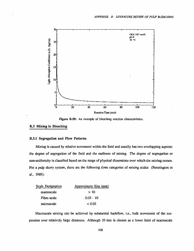
APPENDIX: B: LITERATURE REVIEW OF PULP BLEACHING
002 0.01 mol/LpH 870 °C
60^
80^
100^
120
Reaction Time (min)
Figure B.50: An example of bleaching reaction characteristics.
B.3 Mixing in Bleaching
B.3.1 Segregation and Flow Patterns
Mixing is caused by relative movement within the fluid and usually has two overlapping aspects:
the degree of segregation of the fluid and the earliness of mixing. The degree of segregation or
non-uniformity is classified based on the range of physical dimensions over which the mixing occurs.
For a pulp slurry system, there are the following three categories of mixing scales (Bennington et
al., 1989):
Scale Designation^Approximate Size (mm)macroscale^> 10
Fibre-scale^0.05 - 10
microscale^<0.05
Macroscale mixing can be achieved by substantial backflow, i.e., bulk movement of the sus-
pension over relatively large distances. Although 10 mm is chosen as a lower limit of macroscale
108
APPENDIX: B: LITERATURE REVIEW OF PULP BLEACHING
mixing, dimensions of a pipe diameter or more are of practical interest. Fibre-scale mixing is small
scale mixing achieved primarily by shear, i.e., by local relative fluid movement induced by velocity
gradients or turbulence, and by diffusion, i.e., molecular movement induced by concentration gra-
dients. The other small scale mixing, microscale is mainly attained by molecular diffusion. It is
aided by clump breaking and stretching that greatly increases the surface area available for diffusion.
Uniformities on the three levels, particularly on the small scales depend strongly upon pulp slurry
theology as well as the forces driving mixing such as velocity and concentration gradients.
Pulp slurries are continuous fibre networks that possess structure and strength resulting from
interaction between neighboring fibres. In the slurry having consistencies above 0.5%, cohesive
strength occurs from mechanical forces bending and hooking fibres (Kerekes et al., 1985). At
consistencies above 20%, the character of the slurry changes from mass concentration of fibres in
water to a network of wet fibre aggregates. To produce flow in a pulp slurry or expose fibres to a
chemical at an addition point, sufficient stress must be applied to rupture the fibre network as well as
the flocs within it. Thus, pulp network strength is an important factor in the mixing of pulp slurry.
As the consistency of the slurry increases, the network strength will increase with increase in the
number of fibre to fibre interactions. Flocs with higher local consistency have greater strength than
the surrounding slurry. Kerekes et al. (1985) and many other investigators found that the network
strength is directly proportional to slurry consistency raised to a certain exponent.
The earliness of mixing means whether fluid mixes early or late as it flows through the vessel.
It concerns the bulk flow pattern through the vessel. There are two idealized flow patterns: ideal
mixed flow and plug flow. Though real reactors never fully follow these patterns, a large number of
reactors are designed to approach these ideals with negligible error. For example, tubular vessels can
be considered as plug flow while continuous stirred tank reactors can be accounted for ideal mixed
flow. To characterize the actual flow within a vessel which is neither in plug nor ideally mixed, many
types of non-ideal flow models have been used. Some draw an analogy between mixing in the actual
flow and diffusional process. These are called dispersion models. Others build a chain or network
of ideal mixers. One parameter non-ideal flow models, i.e. the axial dispersed models and CSTRS,
are known as adequate representatives of tubular vessels (Levenspiel, 1972).
109

APPENDIX: B: LITERATURE REVIEW OF PULP BLEACHING
B.3.2 Mixing and Bleaching
Since bleaching involves multiple simultaneous chemical reactions with lignin and carbohydrate
components in the pulp, mixing uniformities as well as flow pattern affect the product quality and
chemical consumption for a desired degree of bleaching. The potential impact of segregation is
dependent on whether the time required for a desirable state in mixing is long or short with respect to
time for bleaching reaction to take place. Relative reaction/mixing rates for major bleaching reactions
in common mixers were obtained by Bennington et al. (1989) and are listed in Table B.15, where
Tr is the inverse of the reaction rate constant, and rm is the time required to produce a mixture of
specific quality, which characterizes mixing rate. Three cases are of interest:
1. Mixing occurs much faster than the reaction rate, rdrm>>1: Here mixing has achieved the
ultimate state in which the chemical agent is uniformly distributed in the bulk liquid around
each fibre before chemical reaction has proceeded to any significant extent. The only remaining
distribution is transfer of the chemical from phase to phase. The overall bleaching rate is therefore
governed by the reaction kinetics. Bleaching with chlorine, chlorine dioxide and oxygen in high-
shear mixer appears to be in this category.
2. Mixing and reaction proceed at approximately the same rate, i.e., rr/rm Here, both mixing
and reaction kinetics determine the bleaching rate.
3. Reaction occurs much faster than mixing, rirm<<1: Here mixing is slow compare to the effective
reaction rate. Consequently, the reaction performance, such as residual chemical, product quality,
is determined by mixing: the rate at which mixing proceeds as well as the degree of the mixture
uniformity. As shown in Table B.15 chlorination in CST falls into this category.
B.33 Bleaching Mixers and Retention Towers
Mixing of pulp slurries is very complex owing to the unique rhe,ology of the slurry caused by
their substantial network strength. The correlation between mixing quality and its factors is not well
known and it is difficult to make direct measurement of this quality. Because each flow pattern of
fluid through the vessel has associated with it a clearly defined residence time distribution (RTD) or
exit age distribution function (E), the flow pattern can be estimated by measurement of residence time
110

APPENDIX: B: LITERATURE REVIEW OF PULP BLEACHING
Table B.15 Relative reaction/mixing rates for common pulp mixers.
Trirm
Bleaching ChemicalsMixer Type
C12 C102 02
CST 6.0x 10⁻² 0.39 4.6
Static 4.5 29 350High-Shear 180 1.2x 10³ 1.4 x 04
distribution (Cholette and Cloutier, 1959; Walker and Cholette, 1958; Reynolds, 1964; Levenspiel,
1972). By comparing the measured E curves with various models, the ability of the mixer to attenuate
incoming fluctuations can be determined and the existence of short circuiting or dead zones within
the vessel can be identified. For pulp mixing, there are a number of methods for assessing macroscale
mixing besides using E curves (Torregrossa, 1983; Pattyson, 1984; Sinn, 1984). A direct measure
of small-scale mixing may be the intensity of segregation (Paterson and Kerekes, 1985; 1986).
However, a quantitative relationship between the behavior of the bleaching process and this small
scale mixing has not been well established while there are various flow pattern models available for
correlating to macroscale mixing.
The flow in bleaching retention towers has been approximated as plug flow. Deviation from
this ideality is sometimes considerable due to channeling, vertical mixing (Snyder, 1966) or creation
of stagnant regions (Perkins, 1986). Mixing behavior in mixers used for bleaching is much more
complex since the initial mixing between the chemical and fibre occurs here while the retention
tower provides the additional time to complete the distribution of chemical throughout the slurry not
accomplished by the mixer, and additional diffusion into the interstices of the fibre. The mixing
behavior of typical bleaching mixers, CST, static mixers and high-shear mixers has been evaluated
by Bennington et al. (1989). The flow pattern in these mixers changes from baclunixing to plug
flow. CST for low consistency pulp produces good macroscale mixing through sufficient bacicmixing,
but with non-uniform fibre-scale mixing. The static and high-shear mixers improve the fibre-scale
uniformity, but at the expense of macroscale mixing.
111