inventory control models - Canvas

INVENTORY CONTROL MODELS

L E A R N I N G O B J E C T I V E S

After completing this chapter, students will be able to:

1. Understand the importance of inventory control.

2. Use inventory control models to determine how muchto order or produce and when to order or produce.

3. Understand inventory models that allow quantity discounts.

4. Understand the use of safety stock with known and unknown stockout costs.

5. Understand the importance of ABC inventory analysis.

6. Use Excel to analyze a variety of inventory control models.

Summary • Glossary • Solved Problems • Discussion Questions andProblems • Case Study: Sturdivant Sound Systems • Case Study: Martin-Pullin Bicycle Corporation • Internet Case Studies • Bibliography

C H A P T E R O U T L I N E

12.1 Introduction

12.2 Importance of Inventory Control

12.3 Inventory Control Decisions

12.4 Economic Order Quantity: Determining How Much to Order

12.5 Reorder Point: Determining When to Order

12.6 Economic Production Quantity: Determining How Much to Produce

12.7 Quantity Discount Models

12.8 Use of Safety Stock

12.9 ABC Analysis

C H A P T E R 12

INVENTORY CONTROL MODELS

12-2 CHAPTER 12 Inventory Control Models

Inventory is any storedresource that is used to satisfya current or future need.

Planning on WhatInventory to

Stock and How toAcquire It

ForecastingParts/Product

Demand

ControllingInventory

Levels

Feedback Measurementsto Revise Plans and

Forecasts

F I G U R E 1 2 . 1

Inventory Planning and Control

12.1 INTRODUCTIONInventory is one of the most expensive and important assets of many companies, repre-senting as much as 50% of total invested capital. Managers have long recognized that goodinventory control is crucial. On one hand, a firm can try to reduce costs by reducing on-hand inventory levels. On the other hand, customers become dissatisfied when frequentinventory outages, called stockouts, occur. Thus, companies must make the balance betweenlow and high inventory levels. As you would expect, cost minimization is the major factorin obtaining this delicate balance.

Inventory is any stored resource that is used to satisfy a current or future need. Rawmaterials, work-in-process, and finished goods are examples of inventory. Inventory levelsfor finished goods, such as clothes dryers, are a direct function of market demand. By usingthis demand information, it is possible to determine how much raw materials (for example,sheet metal, paint, and electric motors in the case of clothes dryers) and work-in-processare needed to produce the finished product.

Every organization has some type of inventory planning and control system. A bank hasmethods to control its inventory of cash. A hospital has methods to control blood suppliesand other important items. State and federal governments, schools, and virtually every man-ufacturing and production organization are concerned with inventory planning and con-trol. Studying how organizations control their inventory is equivalent to studying how theyachieve their objectives by supplying goods and services to their customers. Inventory is thecommon thread that ties all the functions and departments of the organization together.

Figure 12.1 illustrates the basic components of an inventory planning and control sys-tem. The planning phase involves primarily what inventory is to be stocked and how it is tobe acquired (whether it is to be manufactured or purchased). This information is then usedin forecasting demand for the inventory and in controlling inventory levels. The feedbackloop in Figure 12.1 provides a way of revising the plan and forecast based on experiencesand observation.

Through inventory planning, an organization determines what goods and/or servicesare to be produced. In cases of physical products, the organization must also determinewhether to produce these goods or to purchase them from another manufacturer. Whenthis has been determined, the next step is to forecast the demand. As discussed in Chapter11, many mathematical techniques can be used in forecasting demand for a particularproduct. The emphasis in this chapter is on inventory control—that is, how to maintainadequate inventory levels within an organization to support a production or procurementplan that will satisfy the forecasted demand.

In this chapter, we discuss several different inventory control models that are com-monly used in practice. For each model, we provide examples of how they are analyzed.Although we show the equations needed to compute the relevant parameters for each

12.2: Importance of Inventory Control 12-3

Using an Inventory Model to Reduce Costs for a Hewlett-Packard Printer➠MODELING IN THE REAL WORLD

In making products for different markets, manufacturing companies often produce basic products andmaterials that can be used in a variety of end products. Hewlett-Packard, a leading manufacturer of print-ers, wanted to explore ways of reducing material and inventory costs of its Deskjet line of printers. Onespecific problem is that different power supplies are required in different countries.

The inventory model investigates inventory and material requirements as they relate to different markets.An inventory and materials flow diagram was developed that showed how each Deskjet printer was to bemanufactured for various countries requiring different power supplies.

The input data consisted of inventory requirements, costs, and product versions. Different Deskjet ver-sions are needed for the U.S. market, European markets, and Far East markets. The data included esti-mated demand in weeks of supply, replenishment lead times, and various cost data.

The solution resulted in tighter inventory control and a change in how the printer was manufactured. Thepower supply was to be one of the last components installed in each Deskjet during the manufacturingprocess.

Testing was done by selecting one of the markets and performing a number of tests over a two-monthperiod. The tests included material shortages, downtime profiles, service levels, and various inventoryflows.

The results revealed that an inventory cost savings of 18% could be achieved by using the inventory model.

As a result of the inventory model, Hewlett-Packard decided to redesign how its Deskjet printers are manufactured to reduce inventory costs in meeting a global market for its printers.

Source: H. Lee, et al. “Hewlett-Packard Gains Control of Inventory and Service through Design for Localization,” Interfaces 23, 4(July–August 1993): 1–11.

Definingthe Problem

Developinga Model

AcquiringInput Data

Developinga Solution

Testing theSolution

Analyzingthe Results

and SensitivityAnalysis

Implementingthe Results

FORM

ULAT

ION

SOLU

TION

INTE

RPRE

TATI

ON

There are five main uses of inventory.

model, we use Excel worksheets (included on the CD-ROM that accompanies this texbook)to actually calculate these values.

12.2 IMPORTANCE OF INVENTORY CONTROLInventory control serves several important functions and adds a great deal of flexibility tothe operation of a firm. Five main uses of inventory are as follows:

1. The decoupling function

2. Storing resources


Inventory can help avoidstockouts.

Inventory can act as a buffer.

Resources can be stored inwork-in-process.

Inventory helps when there isirregular supply or demand.

Purchasing in large quantitiesmay lower unit costs.

3. Irregular supply and demand

4. Quantity discounts

5. Avoiding stockouts and shortages

Decoupling FunctionOne of the major functions of inventory is to decouple manufacturing processes within theorganization. If a company did not store inventory, there could be many delays and ineffi-ciencies. For example, when one manufacturing activity has to be completed before a sec-ond activity can be started, it could stop the entire process. However, stored inventorybetween processes could act as a buffer.

Storing ResourcesAgricultural and seafood products often have definite seasons over which they can be har-vested or caught, but the demand for these products is somewhat constant during the year.In these and similar cases, inventory can be used to store these resources.

In a manufacturing process, raw materials can be stored by themselves, as work-in-process, or as finished products. Thus, if your company makes lawn mowers, you mightobtain lawn mower tires from another manufacturer. If you have 400 finished lawn mowersand 300 tires in inventory, you actually have 1,900 tires stored in inventory. Three hundredtires are stored by themselves, and 1,600 (= 4 tires per lawn mower × 400 lawn mowers)tires are stored on the finished lawn mowers. In the same sense, labor can be stored ininventory. If you have 500 subassemblies and it takes 50 hours of labor to produce eachassembly, you actually have 25,000 labor hours stored in inventory in the subassemblies. Ingeneral, any resource, physical or otherwise, can be stored in inventory.

Irregular Supply and DemandWhen the supply or demand for an inventory item is irregular, storing certain amounts ininventory can be important. If the greatest demand for Diet-Delight beverage is during thesummer, the Diet-Delight company will have to make sure there is enough supply to meetthis irregular demand. This might require that the company produce more of the soft drinkin the winter than is actually needed in order to meet the winter demand. The inventorylevels of Diet-Delight will gradually build up over the winter, but this inventory will beneeded in the summer. The same is true for irregular supplies.

Quantity DiscountsAnother use of inventory is to take advantage of quantity discounts. Many suppliers offerdiscounts for large orders. For example, an electric jigsaw might normally cost $10 per unit.If you order 300 or more saws at one time, your supplier may lower the cost to $8.75.Purchasing in larger quantities can substantially reduce the cost of products. There are,however, some disadvantages of buying in larger quantities. You will have higher storagecosts and higher costs due to spoilage, damaged stock, theft, insurance, and so on.Furthermore, if you invest in more inventory, you will have less cash to invest elsewhere.

Avoiding Stockouts and ShortagesAnother important function of inventory is to avoid shortages or stockouts. If a company isrepeatedly out of stock, customers are likely to go elsewhere to satisfy their needs. Lostgoodwill can be an expensive price to pay for not having the right item at the right time.

12.4: Economic Order Quantity: Determining How Much to Order 12-5

The purpose of all inventorymodels is to minimizeinventory costs.

Components of total cost.

ORDERING COST FACTORS CARRYING COST FACTORS

Developing and sending purchase orders Cost of capital

Processing and inspecting incoming inventory Taxes

Bill paying Insurance

Inventory inquiries Spoilage

Utilities, phone bills, and so on for the purchasing Theftdepartment

Salaries and wages for purchasing department employees Obsolescence

Supplies such as forms and paper for the Salaries and wages for warehousepurchasing department employees

Utilities and building costs for thewarehouse

Supplies such as forms and papersfor the warehouse

T A B L E 1 2 . 1

Inventory Cost Factors

12.3 INVENTORY CONTROL DECISIONSEven though there are literally millions of different types of products manufactured in oursociety, there are only two fundamental decisions that you have to make when controllinginventory:

1. How much to order

2. When to order

The purpose of all inventory models is to determine how much to order and when toorder. As you know, inventory fulfills many important functions in an organization. But asthe inventory levels go up to provide these functions, the cost of storing and holding inven-tory also increases. Thus, we must reach a fine balance in establishing inventory levels. Amajor objective in controlling inventory is to minimize total inventory costs. Some of themost significant inventory costs are as follows:

1. Cost of the items

2. Cost of ordering

3. Cost of carrying, or holding, inventory

4. Cost of stockouts

5. Cost of safety stock, the additional inventory that may be held to help avoid stockouts

The inventory models discussed in the first part of this chapter assume that demandand the time it takes to receive an order are known and constant, and that no quantity dis-counts are given. When this is the case, the most significant costs are the cost of placing anorder and the cost of holding inventory items over a period of time. Table 12.1 provides alist of important factors that make up these costs. Later in this chapter we discuss severalmore sophisticated inventory models.

12.4 ECONOMIC ORDER QUANTITY: DETERMINING HOW MUCH TO ORDERThe economic order quantity (EOQ) model is one of the oldest and most commonly knowninventory control techniques. Research on its use dates back to a 1915 publication by FordW. Harris. This model is still used by a large number of organizations today. This technique


Assumptions of the EOQmodel.

The inventory usage curve hasa sawtooth shape in the EOQmodel.

Milton Bradley, a division of Hasbro, Inc., has been manufac-turing toys for more than 100 years. Founded by MiltonBradley in 1860, the company started by making a lithographof Abraham Lincoln. Using his printing skills, Bradley devel-oped games and toys, including the Game of Life, Chutes andLadders, Candy Land, Scrabble, and Lite Brite. Today, the company produces hundreds of games, requiring billions ofplastic parts.

When Milton Bradley has determined the optimal quanti-ties for its production runs, it must implement these quantities.Some games require literally hundreds of plastic parts, includ-ing spinners, hotels, people, animals, cars, and so on. Accordingto Gary Brennan, director of manufacturing, getting the rightnumber of pieces to the right toys and production lines is themost important issue for the credibility of the company. Somecompanies, including Wal-Mart, can require 20,000 or moreperfectly assembled games delivered to their warehouses in amatter of days.

Not getting the correct number of parts and pieces is veryfrustrating for customers. It can also be time-consuming, expen-sive, and frustrating for Milton Bradley to supply the extra partsor get returned toys or games. If shortages are found during theassembly stage, the entire production run can be stopped untilthe problem is corrected. Counting parts by hand or machine wasalways problematic and not always accurate. As a result, MiltonBradley decided to weigh the pieces and complete games to deter-mine whether the correct number of parts had been included. Ifthe weight is not exactly correct, there is a problem that needs tobe resolved before the game or toy is packaged or shipped. Usinghighly accurate digital scales, Milton Bradley has been able to getthe right parts to the right production line at the right time.Without this simple implementation approach, the most sophis-ticated production run results would be meaningless.

Source: D. Smock. “Games Tip the Scale at Milton Bradley,” Plastics World(March 1997): 22–26.

IN ACTION Implementing Speed and Quality in the Production Run at Milton Bradley

is relatively easy to use, but it makes a number of assumptions. Some of the more impor-tant assumptions follow:

1. Demand is known and constant.

2. The lead time—that is, the time between the placement of the order and the receipt ofthe order—is known and constant.

3. The receipt of inventory is instantaneous. In other words, the inventory from anorder arrives in one batch, at one point in time.

4. Quantity discounts are not possible.

5. The only variable costs are the cost of placing an order, ordering cost, and the cost ofholding or storing inventory over time, carrying, or holding, cost.

6. If orders are placed at the right time, stockouts and shortages can be avoided completely.

With these assumptions, inventory usage has a sawtooth shape, as in Figure 12.2. Here,Q represents the amount that is ordered. If this amount is 500 units, all 500 units arrive atone time when an order is received. Thus, the inventory level jumps from 0 to 500 units. Ingeneral, the inventory level increases from 0 to Q units when an order arrives.

Because demand is constant over time, inventory drops at a uniform rate over time.(Refer to the sloped line in Figure 12.2.) Another order is placed such that when the inven-tory level reaches 0, the new order is received and the inventory level again jumps to Qunits, represented by the vertical lines. This process continues indefinitely over time.

Ordering and Inventory CostsThe objective of most inventory models is to minimize the total cost. With the assumptionsjust given, the significant costs are the ordering cost and the inventory carrying cost. Allother costs, such as the cost of the inventory itself, are constant. Thus, if we minimize thesum of the ordering and carrying costs, we also minimize the total cost.


0

Q

InventoryLevel

MinimumInventory

Time

Order Quantity = Q =Maximum Inventory Level

F I G U R E 1 2 . 2

Inventory Usage over Time

The objective of the simpleEOQ model is to minimizeordering and carrying costs.

Cost

MinimumTotalCost

Curve for Total Costof Carryingand Ordering

Carrying Cost Curve

Ordering Cost Curve

Order Quantityin Units

OptimalOrderQuantity (Q*)

F I G U R E 1 2 . 3

Total Cost as a Function of Order Quantity

To help visualize this, Figure 12.3 graphs total cost as a function of the order quantity,Q. As the value of Q increases, the total number of orders placed per year decreases. Hence,the total ordering cost decreases. However, as the value of Q increases, the carrying costincreases because the firm has to maintain larger average inventories.

The optimal order size, Q*, is the quantity that minimizes the total cost. Note in Figure12.3 that Q* occurs at the point where the ordering cost curve and the carrying cost curveintersect. This is not by chance. With this particular type of cost function, the optimalquantity always occurs at a point where the ordering cost is equal to the carrying cost.

Now that we have a better understanding of inventory costs, let us see how we candetermine the value of Q* that minimizes the total cost. In determining the annual carry-ing cost, it is convenient to use the average inventory. Referring to Figure 12.2, we see thatthe on-hand inventory ranges from a high of Q units to a low of zero units, with a uniform

The average inventory level isone-half the maximum level.


I is the annual carrying costexpressed as a percentage ofthe unit cost of the item.

Total cost is a nonlinearfunction of Q.

We determine Q* by settingordering cost equal tocarrying cost.

1 See a recent operations management textbook such as J. Heizer and B. Render. OperationsManagement, 8/e. Upper Saddle River, NJ: Prentice Hall, 2006, for more details of these formulas(and other formulas in this chapter).

rate of decrease between these levels. Thus, the average inventory can be calculated as theaverage of the minimum and maximum inventory levels. That is,

Average inventory level = (0 + Q)/2 = Q/2 (12-1)

We multiply this average inventory by a factor called the annual inventory carrying cost perunit to determine the annual inventory cost.

Finding the Economic Order QuantityWe pointed out that the optimal order quantity, Q*, is the point that minimizes the totalcost, where total cost is the sum of ordering cost and carrying cost. We also indicatedgraphically that the optimal order quantity was at the point where the ordering cost wasequal to the carrying cost. Let us now define the following parameters:

The unit carrying cost, Ch, is usually expressed in one of two ways, as follows:

1. As a fixed cost. For example, Ch is $0.50 per unit per year.

2. As a percentage (typically denoted by I) of the item’s unit cost or price. For example,Ch is 20% of the item’s unit cost. In general,

Ch = I × P (12-2)

For a given order quantity Q, the ordering, holding, and total costs can be computed usingthe following formulas:1

(12-3)

(12-4)

(12-5)

Observe that the total purchase cost (i.e., P × D) does not depend on the value of Q. This isso because regardless of how many orders we place each year, or how many units we ordereach time, we will still incur the same annual total purchase cost.

The presence of Q in the denominator of the first term makes Equation 12-5 anonlinear equation with respect to Q. Nevertheless, because the total ordering cost is equalto the total carrying cost at the optimal value of Q, we can set the terms in Equations 12-3and 12-4 equal to each other and calculate the EOQ as

(12-6)Q DC Co h* = ( / )2

Total cost Total ordering cost Total carrying cost Total purchase cost= + += × + × + ×( / ) ( / )D Q C Q C P Do h2

Total carrying cost = ×( / )Q Ch2

Total ordering cost = ×( / )D Q Co

Q* =====

Optimal order quantity (i.e., the EOQ)

Annual demand, in units, for the inventory item

Ordering cost

Carrying or holding cost

of the inventory item

D

C per order

C per unit per year

P Purchase cost per unit

o

h


We use Excel worksheets to doall inventory modelcomputations.

Main menu inExcelModules.

ExcelModules options. SeeAppendix B for details.

This choice appears inExcel’s main menu barwhen ExcelModules is run.

Inventory Modelssubmenu inExcelModules

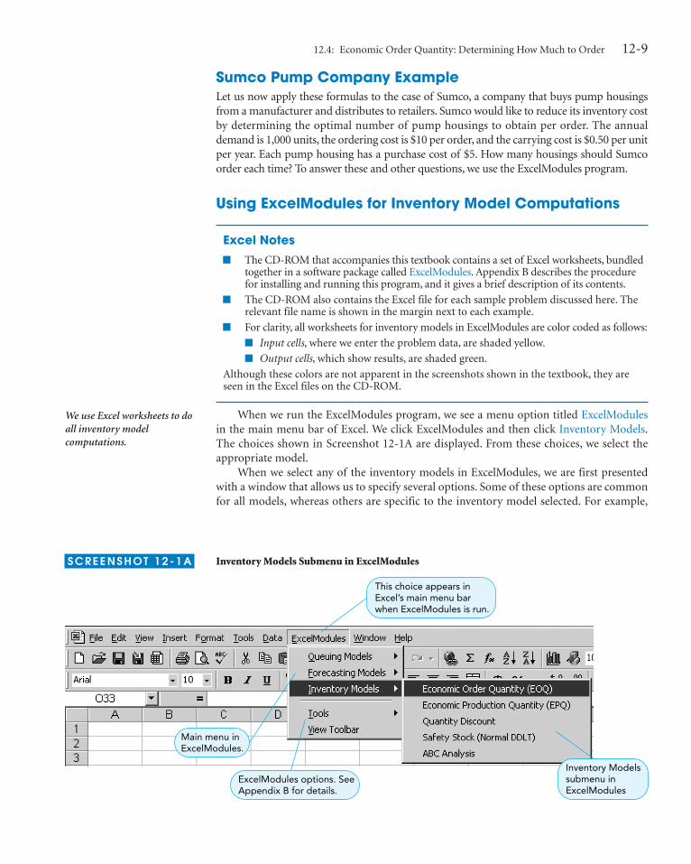
S C R E E N S H OT 1 2 - 1 A Inventory Models Submenu in ExcelModules

Sumco Pump Company ExampleLet us now apply these formulas to the case of Sumco, a company that buys pump housingsfrom a manufacturer and distributes to retailers. Sumco would like to reduce its inventory costby determining the optimal number of pump housings to obtain per order. The annualdemand is 1,000 units, the ordering cost is $10 per order, and the carrying cost is $0.50 per unitper year. Each pump housing has a purchase cost of $5. How many housings should Sumcoorder each time? To answer these and other questions, we use the ExcelModules program.

Using ExcelModules for Inventory Model Computations

Excel Notes� The CD-ROM that accompanies this textbook contains a set of Excel worksheets, bundled

together in a software package called ExcelModules. Appendix B describes the procedurefor installing and running this program, and it gives a brief description of its contents.

� The CD-ROM also contains the Excel file for each sample problem discussed here. Therelevant file name is shown in the margin next to each example.

� For clarity, all worksheets for inventory models in ExcelModules are color coded as follows:

� Input cells, where we enter the problem data, are shaded yellow.

� Output cells, which show results, are shaded green.

Although these colors are not apparent in the screenshots shown in the textbook, they areseen in the Excel files on the CD-ROM.

When we run the ExcelModules program, we see a menu option titled ExcelModulesin the main menu bar of Excel. We click ExcelModules and then click Inventory Models.The choices shown in Screenshot 12-1A are displayed. From these choices, we select theappropriate model.

When we select any of the inventory models in ExcelModules, we are first presentedwith a window that allows us to specify several options. Some of these options are commonfor all models, whereas others are specific to the inventory model selected. For example,


File: 12-2.xls, sheet: 12-2B

Check here to getplot of costs.

Default problem title

This specifies how carryingor holding cost is entered.

Check here tocompute reorderpoint (see section12.5).

S C R E E N S H OT 1 2 - 1 B Sample Options Window for Inventory Models in ExcelModules

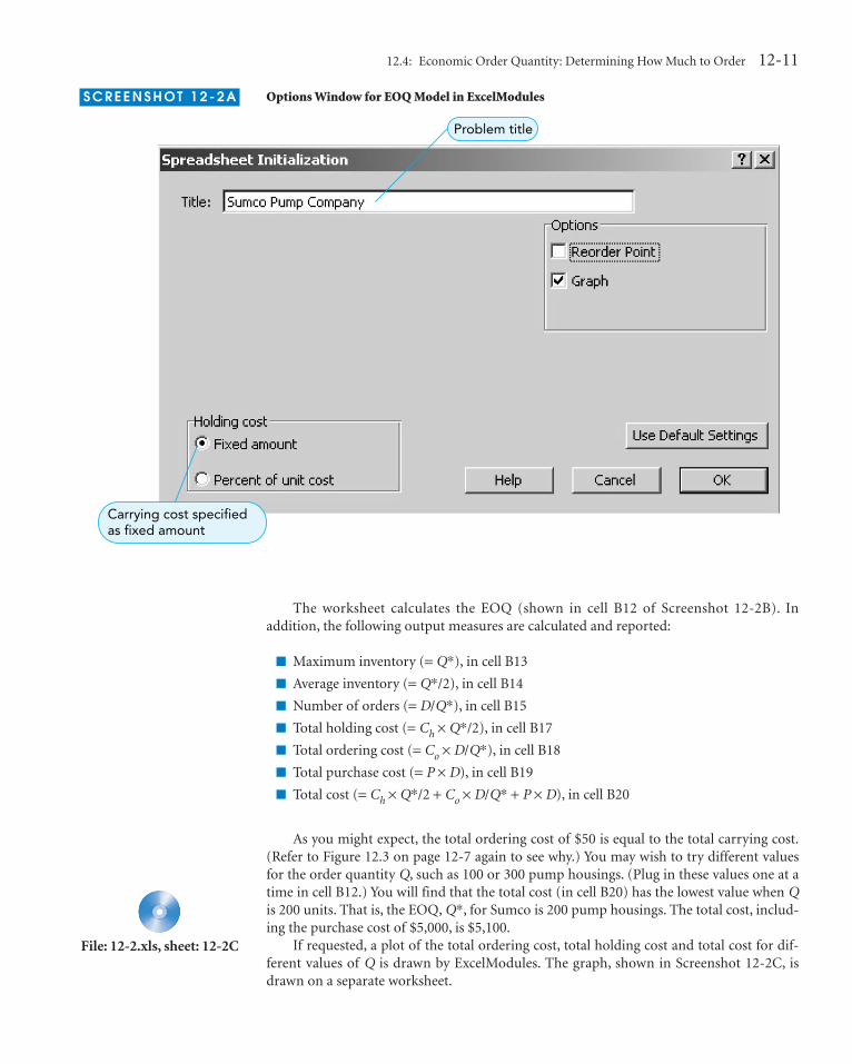
Screenshot 12-1B shows the options window that appears when we select the EconomicOrder Quantity (EOQ) model. The options here include the following:

1. Title of the problem. The default value is Problem Title.

2. Graph. Checking this box results in a graph of ordering, carrying, and total costs ver-sus order quantity.

3. Holding Cost. This is either a fixed amount or a percentage of unit purchase cost.

4. Reorder Point. Checking this box results in the calculation of the reorder point, for agiven lead time between placement of the order and receipt of the order. We discussthe reorder point in section 12.5. This option is available only for the EOQ model.

Using ExcelModules for the EOQ Model Screenshot 12-2A shows the options we selectfor the Sumco Pump Company example.

When we click OK on this screen, we get the worksheet shown in Screenshot 12-2B onpage 12-12. We now enter the values for the annual demand, D, ordering cost, Co, carryingcost, Ch, and unit purchase cost, P, in cells B6 to B9, respectively.

Excel Notes� The worksheets in ExcelModules contain formulas to compute the results for different

inventory models. The default value of zero for the input data causes the results of theseformulas to initially appear as #N/A, #VALUE!, or #DIV/0!. However, as soon as we entervalid values for these input data, the worksheets display the formula results.

� Once ExcelModules has been used to create the Excel worksheet for a particular inven-tory model (e.g., EOQ), the resulting worksheet can be used to compute the results withseveral different input data. For example, we can enter different input data in cells B6:B9of Screenshot 12-2B and compute the results without having to create a new EOQ work-sheet each time.


Carrying cost specifiedas fixed amount

Problem title

S C R E E N S H OT 1 2 - 2 A Options Window for EOQ Model in ExcelModules

File: 12-2.xls, sheet: 12-2C

The worksheet calculates the EOQ (shown in cell B12 of Screenshot 12-2B). In addition, the following output measures are calculated and reported:

� Maximum inventory (= Q*), in cell B13

� Average inventory (= Q*/2), in cell B14

� Number of orders (= D/Q*), in cell B15

� Total holding cost (= Ch × Q*/2), in cell B17

� Total ordering cost (= Co × D/Q*), in cell B18

� Total purchase cost (= P × D), in cell B19

� Total cost (= Ch × Q*/2 + Co × D/Q* + P × D), in cell B20

As you might expect, the total ordering cost of $50 is equal to the total carrying cost.(Refer to Figure 12.3 on page 12-7 again to see why.) You may wish to try different valuesfor the order quantity Q, such as 100 or 300 pump housings. (Plug in these values one at atime in cell B12.) You will find that the total cost (in cell B20) has the lowest value when Qis 200 units. That is, the EOQ, Q*, for Sumco is 200 pump housings. The total cost, includ-ing the purchase cost of $5,000, is $5,100.

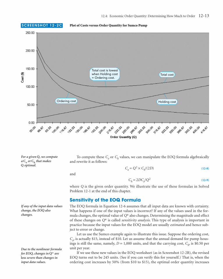
If requested, a plot of the total ordering cost, total holding cost and total cost for dif-ferent values of Q is drawn by ExcelModules. The graph, shown in Screenshot 12-2C, isdrawn on a separate worksheet.


Purchase Cost of Inventory ItemsIt is often useful to know the value of the average inventory level in dollar terms. We knowfrom Equation 12-1 that the average inventory level is Q/2, where Q is the order quantity. Ifwe order Q* (the EOQ) units each time, the value of the average inventory can be com-puted by multiplying the average inventory by the unit purchase cost, P. That is,

Average dollar value of inventory = P × (Q*/2) (12-7)

Calculating the Ordering and Carrying Costs for a Given Value of QRecall that the EOQ formula is given by Equation 12-6 as

In using this formula, we assumed that the values of the ordering cost Co and carrying costCh are known constants. In some situations, however, these costs may be difficult to esti-mate precisely. For example, if the firm orders several items from a supplier simultaneously,it may be difficult to identify the ordering cost separately for each item. In such cases, wecan use the EOQ formula to compute the value of Co or Ch that would make a given orderquantity the optimal order quantity.

Q* ( / )= 2DC Co h

We can calculate the averageinventory value in dollarterms.

EOQ is 200 units.

Data for graph,generated and usedby ExcelModules

Input data

Average inventory = – Maximum inventory

Holding cost = Ordering cost

12

S C R E E N S H OT 1 2 - 2 B EOQ Model for Sumco Pump


For a given Q, we compute a Co or Ch that makes Q optimal.

Total costTotal cost is lowestwhen Holding cost = Ordering cost.

Holding costOrdering cost

S C R E E N S H OT 1 2 - 2 C Plot of Costs versus Order Quantity for Sumco Pump

If any of the input data valueschange, the EOQ alsochanges.

Due to the nonlinear formulafor EOQ, changes in Q* areless severe than changes ininput data values.

To compute these Co or Ch values, we can manipulate the EOQ formula algebraicallyand rewrite it as follows:

Co = Q2 × Ch/(2D) (12-8)

and

Ch = 2DCo/Q2 (12-9)

where Q is the given order quantity. We illustrate the use of these formulas in SolvedProblem 12-1 at the end of this chapter.

Sensitivity of the EOQ FormulaThe EOQ formula in Equation 12-6 assumes that all input data are known with certainty.What happens if one of the input values is incorrect? If any of the values used in the for-mula changes, the optimal value of Q* also changes. Determining the magnitude and effectof these changes on Q* is called sensitivity analysis. This type of analysis is important inpractice because the input values for the EOQ model are usually estimated and hence sub-ject to error or change.

Let us use the Sumco example again to illustrate this issue. Suppose the ordering cost,Co, is actually $15, instead of $10. Let us assume that the annual demand for pump hous-ings is still the same, namely, D = 1,000 units, and that the carrying cost, Ch, is $0.50 perunit per year.

If we use these new values in the EOQ worksheet (as in Screenshot 12-2B), the revisedEOQ turns out to be 245 units. (See if you can verify this for yourself.) That is, when theordering cost increases by 50% (from $10 to $15), the optimal order quantity increases


The ROP determines when toorder inventory.

InventoryLevel(Units)

ROP(Units)

Time(Days)

Q*

Slope = Units/Day = d

Lead Time = L

F I G U R E 1 2 . 4

Reorder Point (ROP)Curve

only by 22.5% (from 200 to 245). This is because the EOQ formula involves a square rootand is, therefore, nonlinear.

We observe a similar occurrence when the carrying cost, Ch, changes. Let us supposethat Sumco’s annual carrying cost is $0.80 per unit, instead of $0.50. Let us also assume thatthe annual demand is still 1,000 units, and the ordering cost is $10 per order. Using theEOQ worksheet in ExcelModules, we can calculate the revised EOQ as 158 units. That is,when the carrying cost increases by 60% (from $0.50 to $0.80), the EOQ decreases by only21%. Note that the order quantity decreases here because a higher carrying cost makesholding inventory more expensive.

12.5 REORDER POINT: DETERMINING WHEN TO ORDERNow that we have decided how much to order, we look at the second inventory question:when to order. In most simple inventory models, it is assumed that receipt of an order isinstantaneous. That is, we assume that a firm waits until its inventory level for a particularitem reaches zero, places an order, and receives the items in stock immediately.

In many cases, however, the time between the placing and receipt of an order, calledthe lead time, or delivery time, is often a few days or even a few weeks. Thus, the when toorder decision is usually expressed in terms of a reorder point (ROP), the inventory level atwhich an order should be placed. The ROP is given as

(12-10)

Figure 12.4 shows the reorder point graphically. The slope of the graph is the daily inven-tory usage. This is expressed in units demanded per day, d. The lead time, L, is the time thatit takes to receive an order. Thus, if an order is placed when the inventory level reaches theROP, the new inventory arrives at the same instant the inventory is reaching zero. Let’s lookat an example.

ROP (Demand per day) (Lead time, in days)= ×= ×d L

12.5: Reorder Point: Determining When to Order 12-15

To compute the ROP, we needto know the demand rate perperiod.

File: 12-3.xls

Input data forcomputing ROP

EOQ is 200 units.

ROP is 12 units.

S C R E E N S H OT 1 2 - 3

EOQ Model with ROP forSumco Pump

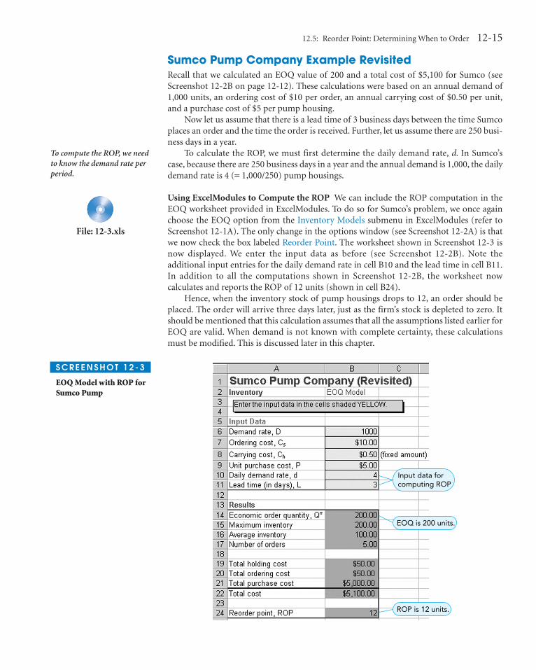
Sumco Pump Company Example RevisitedRecall that we calculated an EOQ value of 200 and a total cost of $5,100 for Sumco (seeScreenshot 12-2B on page 12-12). These calculations were based on an annual demand of1,000 units, an ordering cost of $10 per order, an annual carrying cost of $0.50 per unit,and a purchase cost of $5 per pump housing.

Now let us assume that there is a lead time of 3 business days between the time Sumcoplaces an order and the time the order is received. Further, let us assume there are 250 busi-ness days in a year.

To calculate the ROP, we must first determine the daily demand rate, d. In Sumco’scase, because there are 250 business days in a year and the annual demand is 1,000, the dailydemand rate is 4 (= 1,000/250) pump housings.

Using ExcelModules to Compute the ROP We can include the ROP computation in theEOQ worksheet provided in ExcelModules. To do so for Sumco’s problem, we once againchoose the EOQ option from the Inventory Models submenu in ExcelModules (refer toScreenshot 12-1A). The only change in the options window (see Screenshot 12-2A) is thatwe now check the box labeled Reorder Point. The worksheet shown in Screenshot 12-3 isnow displayed. We enter the input data as before (see Screenshot 12-2B). Note theadditional input entries for the daily demand rate in cell B10 and the lead time in cell B11.In addition to all the computations shown in Screenshot 12-2B, the worksheet nowcalculates and reports the ROP of 12 units (shown in cell B24).

Hence, when the inventory stock of pump housings drops to 12, an order should beplaced. The order will arrive three days later, just as the firm’s stock is depleted to zero. Itshould be mentioned that this calculation assumes that all the assumptions listed earlier forEOQ are valid. When demand is not known with complete certainty, these calculationsmust be modified. This is discussed later in this chapter.


The EPQ model eliminatesthe instantaneous receiptassumption.

InventoryLevel

Time

MaximumInventory

t

Part of Inventory CycleDuring Which Production IsTaking Place

There Is No ProductionDuring This Part of theInventory Cycle

F I G U R E 1 2 . 5

Inventory Control and theProduction Process

Sound inventory control involves much more than computingthe EOQ. In most cases, other practical and financial consider-ations must be taken into account to minimize total inventorycosts and to provide tighter control on inventory levels. Bothpractical and financial considerations led Inland Steel to con-sider several inventory policies, including systems contracts.

Inland Steel produces approximately 5.5 million tons ofsteel each year. The steel mill has two blast furnaces that supplysteel to four casting operations. Yet, steel inventory is not thecompany’s only inventory concern. For many large corpora-tions, office equipment, such as scanners, printers, and faxmachines can represent a substantial investment. Furthermore,all steel-processing facilities are controlled through computers,which are considered office equipment by Inland Steel.

Tricia Wynn, a project buyer for Inland Steel, was con-cerned about high costs and a lack of standardization for office

equipment. To overcome these problems, she developed a com-prehensive inventory ordering system that took advantage ofstandardization and contract buying. The result was a contractordering system that provided superior equipment at substan-tial savings. Most of the equipment was leased or rented. Thenew system provided low monthly rates for office equipment,free installation, and a 30-day free trial. Another advantage wasa floating systems contract. With this type of contract, there isno termination date, which helps reduce the time and costs ofmaintaining leasing agreements. The bottom line is that a sys-tems contract approach allowed Inland Steel to order good-quality office equipment for fewer dollars.

Source: K. Evans-Correia. “All Systems Go,” Purchasing (March 23, 1989):106–107.

IN ACTION Inland Steel Uses Systems Contracts to Control Inventory Costs

12.6 ECONOMIC PRODUCTION QUANTITY: DETERMINING HOW MUCH TO PRODUCE

In the EOQ model, we assumed that the receipt of inventory is instantaneous. In other words,the entire order arrives in one batch, at a single point in time. In many cases, however, a firmmay build up its inventory gradually over a period of time. For example, a firm may receiveshipments from its supplier uniformly over a period of time. Or, a firm may be producing at arate of p per day and simultaneously selling at a rate of d per day (where p > d). Figure 12.5shows inventory levels as a function of time in these situations. Clearly, the EOQ model is nolonger applicable here, and we need a new model to calculate the optimal order (or produc-tion) quantity. Because this model is especially suited to the production environment, it is alsocommonly known as the production lot size model or the economic production quantity (EPQ)model. We refer to this model as the EPQ model in the remainder of this chapter.

In a production process, instead of having an ordering cost, there will be a setup cost. Thisis the cost of setting up the production facility to manufacture the desired product. It nor-mally includes the salaries and wages of employees who are responsible for setting up theequipment, engineering and design costs of making the setup, and the costs of paperwork,supplies, utilities, and so on. The carrying cost per unit is composed of the same factors as thetraditional EOQ model, although the equation to compute the annual carrying cost changes.

12.6: Economic Production Quantity: Determining How Much to Produce 12-17

This is the formula foraverage inventory in the EPQ model.

Here is the formula for theoptimal production quantity.Notice the similarity to thebasic EOQ model.

File: 12-4.xls, sheet: 12-4A

In determining the annual carrying cost for the EPQ model, it is again convenient touse the average on-hand inventory. Referring to Figure 12.5, we can show that the maxi-mum on-hand inventory is Q × (1 � d/p) units, where d is the daily demand rate and p isthe daily production rate. The minimum on-hand inventory is again zero units, and theinventory decreases at a uniform rate between the maximum and minimum levels. Thus,the average inventory can be calculated as the average of the minimum and maximuminventory levels. That is,

Average inventory level = [0 + Q × (1 – d/p)]/2 = Q × (1 – d/p)/2 (12-11)

Analogous to the EOQ model, it turns out that the optimal order quantity in the EPQmodel also occurs when the total setup cost equals the total carrying cost. You should note,however, that making the total setup cost equal to the total carrying cost does not alwaysguarantee optimal solutions for models more complex than the EPQ model.

Finding the Economic Production QuantityLet us first define the following additional parameters:

For a given order quantity, Q, the setup, holding, and total costs can now be computedusing the following formulas:

(12-12)

(12-13)

(12-14)

As in the EOQ model, the total production (or purchase, if the item is purchased) cost doesnot depend on the value of Q. Further, the presence of Q in the denominator of the firstterm makes the total cost function nonlinear. Nevertheless, because the total setup costshould equal the total ordering cost at the optimal value of Q, we can set the terms inEquations 12-12 and 12-13 equal to each other and calculate the EPQ as

(12-15)

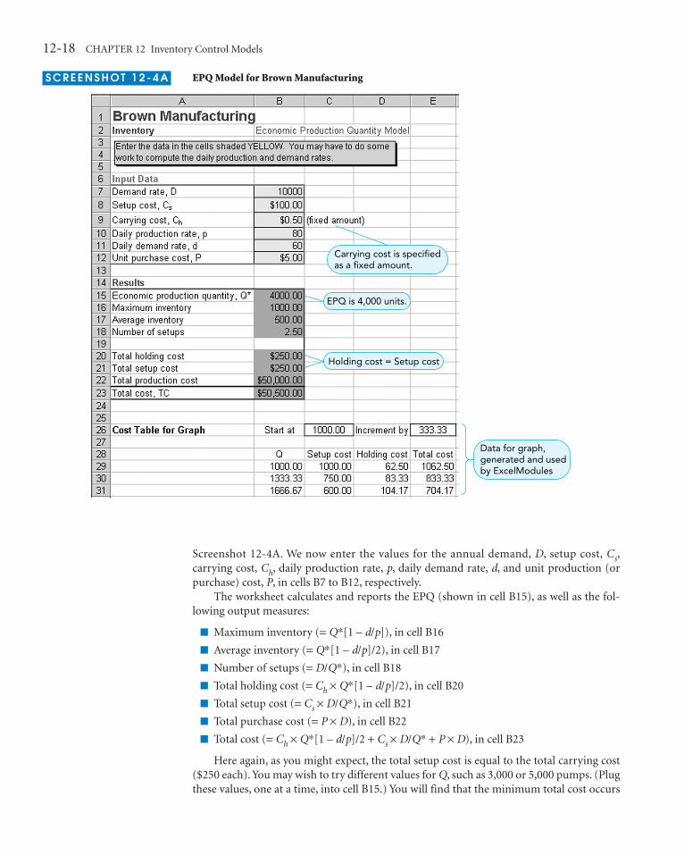
Brown Manufacturing ExampleBrown Manufacturing produces mini-sized refrigeration packs in batches. The firm’s esti-mated demand for the year is 10,000 units. Because Brown operates for 167 business dayseach year, this annual demand translates to a daily demand rate of about 60 units per day. Itcosts about $100 to set up the manufacturing process, and the carrying cost is about $0.50per unit per year. When the production process has been set up, 80 refrigeration packs canbe manufactured daily. Each pack costs $5 to produce. How many packs should Brownproduce in each batch? As discussed next, we determine this value, as well as values for theassociated costs, by using ExcelModules.

Using ExcelModules for the EPQ Model We select the Economic Production Quantity(EPQ) option from the Inventory Models submenu in ExcelModules (refer to Screenshot12-1A). The options for this procedure are similar to those for the EOQ model (seeScreenshot 12-2A). The only change is that the ROP option is not available here. After weenter the title and other options for this problem, we get the worksheet shown in

Q DC C d ps h* = −2 1/[ ( / )]

Total cost Total setup cost Total carrying cost Total production cost= + += × + − × + ×( / ) [ ( / )/ ]D Q C Q d p C P Ds h1 2

Total carrying cost = − ×[ ( / )/ ]Q d p Ch1 2

Total setup cost = ×( / )D Q Cs

Q* ==

Optimal order or production quantity (i.e., the EPQ)

Setup cost per setupCs



Holding cost = Setup cost

EPQ is 4,000 units.

Carrying cost is specifiedas a fixed amount.

S C R E E N S H OT 1 2 - 4 A EPQ Model for Brown Manufacturing

Screenshot 12-4A. We now enter the values for the annual demand, D, setup cost, Cs,carrying cost, Ch, daily production rate, p, daily demand rate, d, and unit production (orpurchase) cost, P, in cells B7 to B12, respectively.

The worksheet calculates and reports the EPQ (shown in cell B15), as well as the fol-lowing output measures:

� Maximum inventory (= Q*[1 – d/p]), in cell B16

� Average inventory (= Q*[1 – d/p]/2), in cell B17

� Number of setups (= D/Q*), in cell B18

� Total holding cost (= Ch × Q*[1 – d/p]/2), in cell B20

� Total setup cost (= Cs × D/Q*), in cell B21

� Total purchase cost (= P × D), in cell B22

� Total cost (= Ch × Q*[1 – d/p]/2 + Cs × D/Q* + P × D), in cell B23

Here again, as you might expect, the total setup cost is equal to the total carrying cost($250 each). You may wish to try different values for Q, such as 3,000 or 5,000 pumps. (Plugthese values, one at a time, into cell B15.) You will find that the minimum total cost occurs

12.7: Quantity Discount Models 12-19


Holding cost

Total cost

Setup cost

S C R E E N S H OT 1 2 - 4 B Plot of Costs versus Order Quantity for Brown Manufacturing

Production cycle is the lengthof each manufacturing run.

A discount is a reduced pricefor an item when it ispurchased in large quantities.

when Q is 4,000 units. That is, the EPQ, Q*, for Brown is 4,000 units. The total cost, includ-ing the production cost of $50,000, is $50,500.

If requested, a plot of the total setup cost, holding cost, and total cost for different val-ues of Q is drawn by ExcelModules. This graph, shown in Screenshot 12-4B, is drawn on aseparate worksheet.

Length of the Production CycleReferring to Figure 12.5, we see that the inventory buildup occurs over a period t duringwhich Brown is both producing and selling refrigeration packs. We refer to this period t asthe production cycle. In Brown’s case, if Q* = 4,000 units and we know that 80 units can beproduced daily, the length of each production cycle will be Q* / p = 4,000 / 80 = 50 days.Thus, when Brown decides to produce refrigeration packs, the equipment will be set up tomanufacture the units for a 50-day time span.

12.7 QUANTITY DISCOUNT MODELSTo increase sales, many companies offer quantity discounts to their customers. A quantitydiscount is simply a decreased unit cost for an item when it is purchased in larger quantities.It is not uncommon to have a discount schedule with several discounts for large orders. Atypical quantity discount schedule is shown in Table 12.2.

As can be seen in Table 12.2, the normal cost for the item in this example is $5. When1,000 to 1,999 units are ordered at one time, the cost per unit drops to $4.80, and when thequantity ordered at one time is 2,000 units or more, the cost is $4.75 per unit. As always,


We calculate Q* values foreach discount.

DISCOUNT DISCOUNT DISCOUNT NUMBER QUANTITY DISCOUNT COST

1 0 to 999 0% $5.00

2 1,000 to 1,999 4% $4.80

3 2,000 and over 5% $4.75

T A B L E 1 2 . 2

Quantity DiscountSchedule

Next, we adjust the Q* values.

The total cost curve is brokeninto parts.

Next, we compute total cost.

We select the Q* with thelowest total cost.

management must decide when and how much to order. But with quantity discounts, howdoes a manager make these decisions?

As with other inventory models discussed so far, the overall objective is to minimizethe total cost. Because the unit cost for the third discount in Table 12.2 is lowest, you mightbe tempted to order 2,000 units or more to take advantage of this discount. Placing anorder for that many units, however, might not minimize the total inventory cost. As the dis-count quantity goes up, the item cost goes down, but the carrying cost increases because theorder sizes are large. Thus, the major trade-off when considering quantity discounts isbetween the reduced item cost and the increased carrying cost.

Recall that we computed the total cost (including the total purchase cost) for the EOQmodel as follows (see Equation 12-5):

Next, we illustrate the four-step process to determine the quantity that minimizes thetotal cost. However, we use a worksheet included in ExcelModules to actually compute theoptimal order quantity and associated costs in our example.

Four Steps to Analyze Quantity Discount Models1. For each discount price, calculate a Q* value, using the EOQ formula (Equation 12-6).

In quantity discount EOQ models, the unit carrying cost, Ch, is typically expressed as apercentage (I) of the unit purchase cost (P). That is, Ch = I × P, as discussed inEquation 12-2. As a result, the value of Q* will be different for each discounted price.

2. For any discount level, if the Q* computed in step 1 is too low to qualify for the dis-count, adjust Q* upward to the lowest quantity that qualifies for the discount. Forexample, if Q* for discount 2 in Table 12.2 turns out to be 500 units, adjust this valueup to 1,000 units. The reason for this step is illustrated in Figure 12.6.

As seen in Figure 12.6, the total cost curve for the discounts shown in Table 12.2 isbroken into three different curves. There are separate cost curves for the first (0 ≤ Q ≤999), second (1,000 ≤ Q ≤ 1,999), and third (Q ≥ 2,000) discounts. Look at the total costcurve for discount 2. The Q* for discount 2 is less than the allowable discount range of1,000 to 1,999 units. However, the total cost at 1,000 units (which is the minimumquantity needed to get this discount) is still less than the lowest total cost for discount 1.Thus, step 2 is needed to ensure that we do not discard any discount level that mayindeed produce the minimum total cost. Note that an order quantity computed in step1 that is greater than the range that would qualify it for a discount may be discarded.

3. Using the total cost equation (Equation 12-5), compute a total cost for every Q*determined in steps 1 and 2. If a Q* had to be adjusted upward because it was belowthe allowable quantity range, be sure to use the adjusted Q* value.

4. Select the Q* that has the lowest total cost, as computed in step 3. It will be the orderquantity that minimizes the total cost.

Total cost Total ordering cost Total carrying cost Total purchase cost= + += × + × + ×( / ) ( / )D C C P Do hQ Q 2

12.7: Quantity Discount Models 12-21

TotalCost

$TC Curve forDiscount 1

TC Curve for Discount 2

Q* for Discount 2

TC Curve for Discount 3

0 1,000 2,000

Order Quantity

F I G U R E 1 2 . 6

Total Cost Curve for theQuantity Discount Model

This is an example of thequantity discount model.


Brass Department Store ExampleBrass Department Store stocks toy cars. Recently, the store was given a quantity discountschedule for the cars, as shown in Table 12.2. Thus, the normal cost for the cars is $5. Fororders between 1,000 and 1,999 units, the unit cost is $4.80, and for orders of 2,000 or moreunits, the unit cost is $4.75. Furthermore, the ordering cost is $49 per order, the annualdemand is 5,000 race cars, and the inventory carrying charge as a percentage of cost, I, is 20%, or 0.2. What order quantity will minimize the total cost? We use theExcelModules program to answer this question.

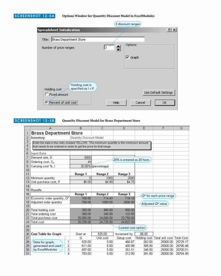
Using ExcelModules for the Quantity Discount Model We select the Quantity Discountoption from the Inventory Models submenu in ExcelModules (refer back to Screenshot 12-1A). The window shown in Screenshot 12-5A is displayed. The option entries in thiswindow are similar to those for the EOQ model (see Screenshot 12-2A). The onlyadditional choice is the box labeled Number of price ranges. The specific entries for BrassDepartment Store’s problem are shown in Screenshot 12-5A.

When we click OK on this screen, we get the worksheet shown in Screenshot 12-5B. Wenow enter the values for the annual demand, D, ordering cost, Co, and holding cost per-centage, I, in cells B7 to B9, respectively. Note that I is entered as a percentage value (e.g.,enter 20 for the Brass Department Store example). Then, for each of the three discountranges, we enter the minimum quantity needed to get the discount and the discounted unitprice, P. These entries are shown in cells B12:D13 of Screenshot 12-5B.

The worksheet works through the four-step process and reports the following outputmeasures for each discount range:

� EOQ value (shown in cells B17:D17), computed using Equation 12-6

� Adjusted EOQ value (shown in cells B18:D18), as discussed in step 2 of the four-stepprocess

� Total holding cost, total ordering cost, total purchase cost, and overall total cost,shown in cells B20:D23


20% is entered as 20 here.

Q* for each price range

Adjusted Q* value

Lowest cost option

S C R E E N S H OT 1 2 - 5 B Quantity Discount Model for Brass Department Store

Holding cost isspecified as I × P.

3 discount ranges

S C R E E N S H OT 1 2 - 5 A Options Window for Quantity Discount Model in ExcelModules

12.8: Use of Safety Stock 12-23

File: 12-5.xls, sheet: 12-5C

Safety stock helps in avoidingstockouts. It is extra stock kepton hand.

In the Brass Department Store example, observe that the Q* values for discounts 2 and3 are too low to be eligible for the discounted prices. They are, therefore, adjusted upwardto 1,000 and 2,000, respectively. With these adjusted Q* values, we find that the lowest totalcost of $24,725 results when we use an order quantity of 1,000 units.

If requested, ExcelModules will also draw a plot of the total cost for different values ofQ. This graph, shown in Screenshot 12-5C, is drawn on a separate worksheet.

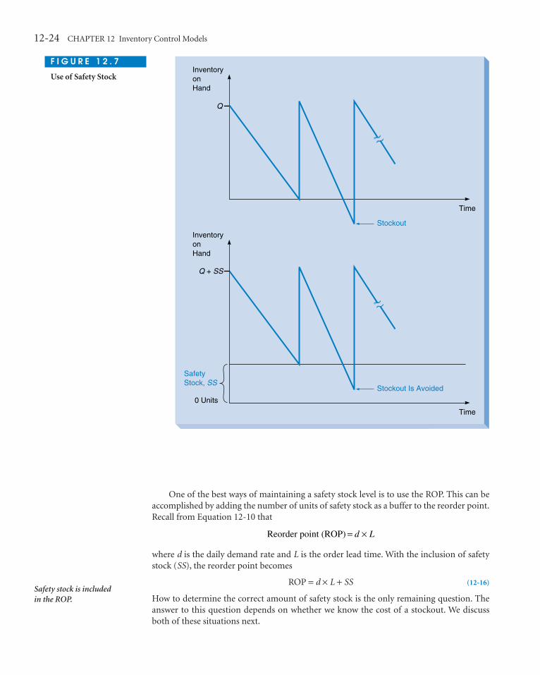
12.8 USE OF SAFETY STOCKSafety stock is additional stock that is kept on hand.2 If, for example, the safety stock for anitem is 50 units, you are carrying an average of 50 units more of inventory during the year.When demand is unusually high, you dip into the safety stock instead of encountering astockout. Thus, the main purpose of safety stock is to avoid stockouts when the demand ishigher than expected. Its use is shown in Figure 12.7. Note that although stockouts canoften be avoided by using safety stock, there is still a chance that they may occur. Thedemand may be so high that all the safety stock is used up, and thus there is still a stockout.

Cost curve for range 1


Minimum cost


S C R E E N S H OT 1 2 - 5 C Plot of Total Cost versus Order Quantity for Brass Department Store

2 Safety stock is used only when demand is uncertain, and models under uncertainty are generallymuch harder to deal with than models under certainty.


InventoryonHand

Time

InventoryonHand

Time

SafetyStock, SS

0 Units

Q

Stockout Is Avoided

Stockout

Q + SS

F I G U R E 1 2 . 7

Use of Safety Stock

Safety stock is included in the ROP.

One of the best ways of maintaining a safety stock level is to use the ROP. This can beaccomplished by adding the number of units of safety stock as a buffer to the reorder point.Recall from Equation 12-10 that

where d is the daily demand rate and L is the order lead time. With the inclusion of safetystock (SS), the reorder point becomes

ROP = d × L + SS (12-16)

How to determine the correct amount of safety stock is the only remaining question. Theanswer to this question depends on whether we know the cost of a stockout. We discussboth of these situations next.

Reorder point (ROP) = ×d L


In many cases, companies buy inventory supplies from severalsuppliers. This was the case with Bellcore, formed in 1984 toallow the regional Bell operating companies to share commonresources. The operating companies, which included Ameritech,Bell Atlantic, BellSouth Telecommunications, NYNEX, PacificBell, Southwestern Bell, and US West are often referred to as Bellclient companies.

By pooling their resources, the Bell client companies haveconsiderable power over their suppliers. As a result, theydecided to select suppliers of required raw materials and inven-tory based on the availability and amount of quantity dis-counts and business volume discounts. Whereas a traditionalquantity discount is based on the amount of a particular inven-tory item that is ordered, a business volume discount is basedon the total dollar value of all items purchased. With a businessvolume discount, the supplier typically discounts each item inan order by the same amount.

One major inventory item needed by the Bell client com-panies is modular circuit boards, so managers of these firmsinquired how they could purchase the boards from Bellcoreunder business volume discounts. The result was a quantitativemodel, called the Procurement Decision Support System(PDSS), that determines the optimal ordering policy based onthe most economical purchase of items under business volumediscounts. PDSS was written to run on personal computers.The program allowed Bell client companies to move away fromquantity discounts toward business volume discounts.

What is the result of using business volume discounts?PDSS now controls inventory and products worth more than$600 million. The savings for Bell client companies haveranged from about $5 million to $15 million per year.

Source: P. Katz, et al. “Telephone Companies Analyze Price Quotations withBellcore’s PDSS Software,” Interfaces 24 (January–February 1994): 50–63.

IN ACTION Telephone Companies Analyze Price Quotations and Quantity Discounts

3 Note that we have assumed that we already know the values of Q* and ROP. If this is not true, thevalues of Q*, ROP, and safety stock would have to be determined simultaneously. This requires amore complex solution.

Safety Stock with Known Stockout CostsWhen the EOQ is fixed and the ROP is used to place orders, the only time a stockout can occur is during the lead time. Recall that the lead time is the time between when anorder is placed and when it is received. In the procedure discussed here, it is necessary toknow the probability of demand during lead time (DDLT) and the cost of a stockout. Inwhat follows, we assume that DDLT follows a discrete probability distribution. Thisapproach, however, can be easily modified when DDLT follows a continuous probabilitydistribution.

What factors should we include in computing the stockout cost per unit? In general,we should include all costs that are a direct or indirect result of a stockout. For example, letus assume that if a stockout occurs, we lose that specific sale forever. Thus, if there is a profitmargin of $1 per unit, we have lost this amount. Furthermore, we may end up losing futurebusiness from customers who are upset about the stockout. An estimate of this cost mustalso be included in the stockout cost.

When we know the probability distribution of DDLT and the cost of a stockout, we candetermine the safety stock level that minimizes the total cost. We illustrate this computa-tion using an example.

ABCO Example ABCO, Inc., uses the EOQ model and ROP analysis (which we saw insections 12.4 and 12.5, respectively) to set its inventory policy. The company hasdetermined that its optimal ROP is 50 (= d × L) units, and the optimal number of ordersper year is 6. ABCO’s DDLT is, however, not a constant. Instead, it follows the probabilitydistribution shown in Table 12.3.3

Loss of goodwill must beincluded in stockout costs.


NUMBER OF UNITS PROBABILITY

30 0.2

40 0.2

ROP → 50 0.3

60 0.2

70 0.1

1.0

T A B L E 1 2 . 3

Probability of DemandDuring Lead Time forABCO, Inc.

Stockout and additionalcarrying costs will be zerowhen ROP = demand duringlead time.

If ROP < DDLT, total cost =total stockout cost.

If ROP > DDLT, total cost =total additional inventorycarrying cost.



Because DDLT is uncertain, ABCO would like to find the revised ROP, including safetystock, which will minimize total expected cost. The total expected cost is the sum ofexpected stockout cost and the expected carrying cost of the additional inventory.

When we know the unit stockout cost and the probability distribution of DDLT, theinventory problem becomes a decision making under risk problem. (Refer to section 8.5 inChapter 8 for a discussion of such problems, if necessary.) For ABCO, the decision alterna-tives are to use an ROP of 30 (alternative 1), 40 (alternative 2), 50 (alternative 3), 60 (alter-native 4), or 70 (alternative 5) units. The outcomes are DDLT values of 30 (outcome 1), 40(outcome 2), 50 (outcome 3), 60 (outcome 4), or 70 (outcome 5) units.

Determining the economic payoffs for any decision alternative and outcome combina-tion involves a careful analysis of the stockout and additional carrying costs. Consider a sit-uation in which the ROP equals the DDLT (say, 30 units each). This means that there willbe no stockouts and no extra units on hand when the new order arrives. Thus, stockoutsand additional carrying costs will be zero. In general, when the ROP equals the DDLT, totalcost will be zero.

Now consider what happens when the ROP is less than the DDLT. For example, saythat ROP is 30 units and DDLT is 40 units. In this case we will be 10 units short. The cost ofthis stockout situation is $2,400 (= 10 units short × $40 per stockout × 6 orders per year).Note that we have to multiply the stockout cost per unit and the number of units short bythe number of orders per year (6, in this case) to determine annual expected stockout cost.Likewise, if the ROP is 30 units and the DDLT is 50 units, the stockout cost will be $4,800(= 20 × $40 × 6), and so on. In general, when the ROP is less than the DDLT, the total costis equal to the total stockout cost.

Finally, consider what happens when the ROP exceeds the DDLT. For example, say thatROP is 70 units and DDLT is 60 units. In this case, we will have 10 additional units on handwhen the new inventory is received. If this situation continues during the year, we will have10 additional units on hand, on average. The additional carrying cost is $50 (= 10 addi-tional units × $5 carrying cost per unit per year). Likewise, if the DDLT is 50 units, we willhave 20 additional units on hand when the new inventory arrives, and the additional carry-ing cost will be $100 (= 20 × $5). In general, when the ROP is greater than the DDLT, totalcost will be equal to the total additional carrying cost.

Using the procedures described previously, we can easily set up a spreadsheet to com-pute the total cost for every alternative and state of nature combination. The formula viewfor this spreadsheet is shown in Screenshot 12-6A.

The results of the analysis are shown in Screenshot 12-6B. The expected monetary val-ues (EMV) in column G show that the best reorder point for ABCO is 70 units, with anexpected total cost of $110. Recall that ABCO had determined its optimal ROP to be 50 units if DDLT was a constant. Hence, the results in Screenshot 12-6B imply that due tothe uncertain nature of DDLT, ABCO should carry a safety stock of 20 (= 70 – 50) units.

We use a decision makingunder risk approach here.


Cost = Stockout cost, if ROP < DDLT

Cost = 0, if ROP = DDLT Expected monetaryvalue of each decisionalternative

Cost = Additionalholding cost, ifROP > DDLT

S C R E E N S H OT 1 2 - 6 A Formula View of Safety Stock Computation for ABCO, Inc.

Best alternativeis ROP = 70.

Probability of each DDLT value

Input data

S C R E E N S H OT 1 2 - 6 B

Safety Stock Computationfor ABCO, Inc.

Determining stockout costsmay be difficult or impossible.

Safety Stock with Unknown Stockout CostsWhen stockout costs are not available or if they are not relevant, the preceding type of analy-sis cannot be used. Actually, there are many situations in which stockout costs are unknownor extremely difficult to determine. For example, let’s assume that you run a small bicycleshop that sells mopeds and bicycles with a one-year service warranty. Any adjustments madewithin the year are done at no charge to the customer. If the customer comes in for mainte-nance under the warranty, and you do not have the necessary part, what is the stockout cost?It cannot be lost profit because the maintenance is done free of charge. Thus, the majorstockout cost is the loss of goodwill. The customer may not buy another bicycle from yourshop if you have a poor service record. In this situation, it could be very difficult to deter-mine the stockout cost. In other cases, a stockout cost may simply not apply. What is thestockout cost for life-saving drugs in a hospital? The drugs may only cost $10 per bottle. Is


We find the Z value for thedesired service level.

A safety stock level isdetermined for each servicelevel.

SS

5% Area of Normal Curve

µ = 350 X = ?

µ = Mean Demand = 350

σ = Standard Deviation = 10

= Mean Demand + Safety StockX

SS = Safety Stock = X µ–

X µ–Z =

σ

F I G U R E 1 2 . 8

Safety Stock and theNormal Distribution

the stockout cost $10? Is it $100 or $10,000? Perhaps the stockout cost should be $1 million.What is the cost when a life may be lost as a result of not having the drug?

In such cases, an alternative approach to determining safety stock levels is to use a ser-vice level. In general, a service level is the percentage of the time that you will have the itemin stock. In other words, the probability of having a stockout is 1 minus the service level.That is,

or

Probability of a stockout = 1 – Service level (12-17)

To determine the safety stock level, it is only necessary to know the probability ofDDLT and the desired service level. Here is an example of how the safety stock level can bedetermined when the DDLT follows a normal probability distribution.

Hinsdale Company Example Hinsdale Company carries an item whose DDLT follows anormal distribution, with a mean of 350 units and a standard deviation of 10 units.Hinsdale wants to follow a policy that results in a service level of 95%. How much safetystock should Hinsdale maintain for this item?

Figure 12.8 may help you to visualize the example. We use the properties of a standard-ized normal curve to get a Z value for an area under the normal curve of 0.95 =(1 – 0.05). Using the normal table in Appendix C on page 637, we find this Z value to be 1.645.

As shown in Figure 12.8, Z is equal to (X – µ)/σ, or SS/σ. Hence, SS is equal to Z × σ.That is, Hinsdale’s safety stock for a service level of 95% is (1.645 × 10) = 16.45 units (whichcan be rounded off to 17 units, if necessary). We can calculate the safety stocks for differentservice levels in a similar fashion.

Let’s assume that Hinsdale has a carrying cost of $1 per unit per year. What is the car-rying cost for service levels that range from 90% to 99.99%? To compute this cost, we firstcompute the safety stock for each service level (as discussed earlier) and then multiply thesafety stock by the unit carrying cost. The Z value, safety stock, and total carrying cost fordifferent service levels for Hinsdale are summarized in Table 12.4. A graph of the total car-rying cost as a function of the service level is given in Figure 12.9.

Service level Probability of a stockout= 1 –An alternative to determiningsafety stock is to use servicelevel and the normaldistribution.


The relationship betweenservice level and carrying costis nonlinear.

SERVICE Z VALUE FROM SAFETY STOCK CARRYING LEVEL NORMAL CURVE TABLE (UNITS) COST

90% 1.28 12.8 $12.80

91% 1.34 13.4 $13.40

92% 1.41 14.1 $14.10

93% 1.48 14.8 $14.80

94% 1.55 15.5 $15.50

95% 1.65 16.5 $16.50

96% 1.75 17.5 $17.50

97% 1.88 18.8 $18.80

98% 2.05 20.5 $20.50

99% 2.33 23.3 $23.20

99.99% 3.72 37.2 $37.20

T A B L E 1 2 . 4

Cost of Different Service Levels

($)40

35

30

25

20

15

10

90 91 92 93 94 95 96

Service Level (%)

Inve

ntor

y C

arry

ing

Cos

ts (

$)

97 98 99 99.99 (%)

F I G U R E 1 2 . 9

Service Level versusAnnual Carrying Costs

Note from Figure 12.9 that the relationship between service level and carrying cost isnonlinear. As the service level increases, the carrying cost increases at an increasing rate.Indeed, at very high service levels, the carrying cost becomes very large. Therefore, as youare setting service levels, you should be aware of the additional carrying cost that you willencounter. Although Figure 12.9 was developed for a specific case, the general shape of thecurve is the same for all service-level problems.



ROP = µ + SS


95% is entered as 95 here.

S C R E E N S H OT 1 2 - 7 A Safety Stock (Normal DDLT) Model for Hinsdale

Using ExcelModules to Compute the Safety Stock We select the Safety Stock (NormalDDLT) option from the Inventory Models submenu in ExcelModules (refer to Screenshot12-1A). The options for this procedure include the problem title and a box to specifywhether we want a graph of carrying cost versus service level. After we specify theseoptions, we get the worksheet shown in Screenshot 12-7A. We now enter values for themean DDLT (µ), standard deviation of DDLT (σ), service level desired, and carrying cost,Ch, in cells B6 to B9, respectively.

The worksheet calculates and displays the following output measures:

� Safety stock, SS (= Z × σ), in cell B12

� Reorder point (= µ + Z × σ), in cell B13

� Safety stock carrying cost (= Ch × Z × σ), in cell B15

If requested, ExcelModules will draw a plot of the safety stock carrying cost for different values of the service level. This graph, shown in Screenshot 12-7B, is drawn on a separate worksheet. As expected, the shape of this graph is the same as that shown inFigure 12.9.


12.9: ABC Analysis 12-31

In a typical manufacturing firm, inventories comprise a bigpart of assets. At the San Miguel Corporation (SMC), whichproduces and distributes more than 300 products to every cor-ner of the Philippine archipelago, raw material accounts forabout 10% of total assets. The significant amount of moneytied up in inventory encouraged the company’s OperationsResearch Department to develop a series of cost-minimizinginventory models.

One major SMC product, ice cream, uses dairy and cheesecurd imported from Australia, New Zealand, and Europe. Thenormal mode of delivery is sea, and delivery frequencies arelimited by supplier schedules. Stockouts, however, are avoid-able through airfreight expediting. SMC’s inventory model for

ice cream balances ordering, carrying, and stockout costs whileconsidering delivery frequency constraints and minimumorder quantities. Results showed that current safety stocks of30–51 days could be cut in half for dairy and cheese curd. Evenwith the increased use of expensive airfreight, SMC saved$170,000 per year through the new policy.

Another SMC product, beer, consists of three major ingre-dients: malt, hops, and chemicals. Because these ingredients arecharacterized by low expediting costs and high unit costs,inventory modeling pointed to optimal policies that reducedsafety stock levels, saving another $180,000 per year.

Source: E. Del Rosario. “Logistical Nightmare,” OR/MS Today (April 1999):44–45. Copyright © 1999. Reprinted with permission.

IN ACTION Inventory Modeling at the San Miguel Corporation in the Phillippines

Cost increases sharplyat this level.

Curve is nonlinear.

S C R E E N S H OT 1 2 - 7 B Plot of Safety Stock Cost versus Service Level for Hinsdale

12.9 ABC ANALYSISSo far, we have shown how to develop inventory policies using quantitative decision models. There are, however, some very practical issues, such as ABC analysis,that should be incorporated into inventory decisions. ABC analysis recognizes the fact


ARE QUANTITATIVE INVENTORY DOLLAR INVENTORY INVENTORY CONTROL

GROUP USAGE ITEMS TECHNIQUES USED?

A 70% 10% Yes

B 20% 20% In some cases

C 10% 70% No

T A B L E 1 2 . 5

Summary of ABC Analysis

File: 12-8.xls

The C group items are not asimportant as the others interms of annual dollar value.

The B group items areimportant but not critical.

The items in the A group arecritical.

that some inventory items are more important than others. The purpose of this analysis is to divide all of a company’s inventory items into three groups: A, B, and C. Then,depending on the group, we decide how the inventory levels should be controlled. A brief description of each group follows, with general guidelines as to which items are A,B, and C.

The inventory items in the A group are critical to the functioning of the company. As aresult, their inventory levels must be closely monitored. These items typically make upmore than 70% of the company’s business in monetary value but only about 10% of allinventory items. That is, a few inventory items are very important to the company. As aresult, the inventory control techniques discussed in this chapter should be used whereappropriate for every item in the A group (see Table 12.5).

The items in the B group are important to the firm but not critical. Thus, it may not benecessary to monitor all these items closely. These items typically represent about 20% ofthe company’s business in monetary value and constitute about 20% of the items in inven-tory. Quantitative inventory models should be used only on some of the B items. The costof implementing and using these models must be carefully balanced with the benefits ofbetter inventory control. Usually, less than half of the B group items are controlled throughthe use of inventory control models.

The items in the C group are not as important to the operation of the company. Theseitems typically represent only about 10% of the company’s business in monetary value butmay constitute 70% of the items in inventory. Group C could include inexpensive itemssuch as bolts, washers, screws, and so on. They are usually not controlled using inventorycontrol models because the cost of implementing and using such models would far exceedthe value gained.

We illustrate the use of ABC analysis using the example of Silicon Chips, Inc.

Silicon Chips, Inc., ExampleSilicon Chips, Inc., maker of super-fast DRAM chips, has organized its 10 inventory itemson an annual dollar-volume basis. Table 12.6 shows the items (identified by the item num-ber and part number), their annual demands, and unit costs. How should the companyclassify these items into groups A, B, and C? As discussed next, we use the worksheet pro-vided in ExcelModules to answer this question.

Using ExcelModules for ABC Analysis We select the ABC Analysis option from theInventory Models submenu in ExcelModules (refer to Screenshot 12-1A). The options forthis procedure include the problem title and boxes to specify the number and names of theitems we want to classify. After we specify these options for the Silicon Chips example, weget the worksheet shown in Screenshot 12-8. We now enter the volume and unit cost foreach item in cells B7:C16 of this worksheet.

ITEM NUMBER PART NUMBER ANNUAL VOLUME (UNITS) UNIT COST

Item 1 01036 100 $ 8.50

Item 2 01307 1,200 $ 0.42

Item 3 10286 1,000 $ 90.00

Item 4 10500 1,000 $ 12.50

Item 5 10572 250 $ 0.60

Item 6 10867 350 $ 42.86

Item 7 11526 500 $154.00

Item 8 12572 600 $ 14.17

Item 9 12760 1,550 $ 17.00

Item 10 14075 2,000 $ 0.60

T A B L E 1 2 . 6

Inventory Data for SiliconChips, Inc.

Sorted values ofpercentage $ volume

Input data

Click this button after entering all input data.

Items are sorted indescending order ofpercentage $ volume.

2 items

3 items

5 items

A

B

C

S C R E E N S H OT 1 2 - 8 ABC Analysis for Silicon Chips, Inc.


Teradyne, a huge manufacturer of electronic testing equipment forsemiconductor plants worldwide, recently asked the WhartonSchool of Business to evaluate its global inventory parts system.Teradyne’s system is complex because it stocks over 10,000 partswith a wide variety of prices (from a few dollars to $10,000)because its customers are dispersed all over the world, and becausecustomers demand immediate response when a part is needed.

The professors selected two basic inventory models theyfelt could be used to improve the current inventory systemeffectively. An important consideration in using basic inven-tory models is their simplicity, which improved the professors’communication with Teradyne executives. In the field of mod-eling, it is very important for managers who depend on themodels to thoroughly understand the underlying processes anda model’s limitations.

Input data to the inventory models included actualplanned inventory levels, holding costs, observed demandrates, and estimated lead times. The outputs included servicelevels and a prediction of the expected number of late partshipments. The first inventory model showed that Teradynecould reduce late shipments by over 90% with just a 3%increase in inventory investment. The second model showedthat the company could reduce inventory by 37% whileimproving customer service levels by 4%.

Source: M. A. Cohen, Y. Zheng, and Y. Wang. “Identifying Opportunities forImproving Teradyne’s Service Parts Logistics System,” Interfaces (July–August1999): 1–18.

IN ACTION Inventory Modeling at Teradyne

Items are sorted in descendingorder of percentage dollarvolume.

When we enter the input data, the worksheet computes the dollar volume and per-centage dollar volume (based on total dollar volume) for each item. These values are shownin cells E7:F16 of Screenshot 12-8. After entering the data for all items, we click the Analyze button. The worksheet now sorts the items, in descending order of percentage dollar volume. These values are shown in descending order in cells F21:F30 ofScreenshot 12-8.

The sorted results for the Silicon Chips, Inc., problem are shown in cells A21:C30 ofScreenshot 12-8. Items 3 and 7, which constitute only 20% (= 2/10) of the total number ofitems, account for 71.97% of the total dollar volume of all items. These two items shouldtherefore be classified as group A items.

Items 9, 6, and 4, which constitute 30% (= 3/10) of the total number of items, accountfor 23.20% (= 95.17 – 71.97) of the total dollar volume of all items. These three itemsshould therefore be classified as group B items.

The remaining items constitute 50% (= 5/10) of the total number of items. However,they account for only 4.83% (= 100 – 95.17) of the total dollar volume of all items. Thesefive items should therefore be classified as group C items.

SUMMARYThis chapter presents several inventory models and discusses how we can use ExcelModules to analyze thesemodels. The focus of all models is to answer the same two primary questions in inventory planning: (1) howmuch to order and (2) when to order. The basic EOQ inven-tory model makes a number of assumptions: (1) knownand constant demand and lead times, (2) instantaneousreceipt of inventory, (3) no quantity discounts, (4) nostockouts or shortages, and (5) the only variable costs areordering costs and carrying costs. If these assumptions arevalid, the EOQ inventory model provides optimal

solutions. If these assumptions do not hold, more complexmodels are needed. For such cases, the economic produc-tion quantity and quantity discount models are necessary.We also discuss the computation of safety stocks whendemand during lead time is unknown for two cases: (1) costof stockout is known and (2) cost of stockout is unknown.Finally, we present ABC analysis to determine how inven-tory items should be classified based on their importanceand value. For all models discussed in this chapter, we show how Excel worksheets can be used to perform thecomputations.

Solved Problems 12-35

GLOSSARYABC Analysis. An analysis that divides inventory into three

groups: Group A is more important than group B, which ismore important than group C.

Average Inventory. The average inventory on hand. Computedas (Maximum inventory + Minimum inventory)/2.

Carrying Cost. The cost of holding one unit of an item in inven-tory for one period (typically a year). Also called holding cost.

Demand During Lead Time (DDLT). The demand for an itemduring the lead time, between order placement and order receipt.

Economic Order Quantity (EOQ). The amount of inventoryordered that will minimize the total inventory cost. It is alsocalled the optimal order quantity, or Q*.

Economic Production Quantity (EPQ) Model. An inventorymodel in which the instantaneous receipt assumption has beeneliminated. The inventory build-up, therefore, occurs over aperiod of time.

Instantaneous Inventory Receipt. A system in which inventoryis received or obtained at one point in time and not over aperiod of time.

Lead Time. The time it takes to receive an order after it is placed.

Ordering Cost. The cost of placing an order.

Purchase Cost. The cost of purchasing one unit of an inventoryitem.

Quantity Discount. The cost per unit when large orders of aninventory item are placed.

Reorder Point (ROP). The number of units on hand when anorder for more inventory is placed.

Safety Stock. Extra inventory that is used to help avoid stockouts.

Safety Stock with Known Stockout Costs. An inventory modelin which the probability distribution of DDLT and the unitstockout cost are known.

Safety Stock with Unknown Stockout Costs. An inventorymodel in which the probability distribution of DDLT is known.The stockout cost is, however, not known.

Service Level. The chance, expressed as a percentage, that there willnot be a stockout. Service level = 1 – Probability of a stockout.

Setup Cost. The cost to set up the manufacturing or productionprocess.

Stockout. A situation that occurs when there is no inventory onhand.

Total Cost. The sum of the total ordering, total carrying, andtotal purchasing costs.

SOLVED PROBLEMS

Solved Problem 12-1Patterson Electronics supplies microcomputer circuitry to a company that incorporates microprocessorsinto refrigerators and other home appliances. Currently, Patterson orders a particular component inbatches of 300 units from one of its suppliers. The annual demand for this component is 2,000.

a. If the carrying cost is estimated at $1 per unit per year, what would the ordering cost have to be tomake the order quantity optimal?

b. If the ordering cost is estimated to be $50 per order, what would the carrying cost have to be tomake the order quantity optimal?

Solutiona. Recall from Equation 12-8 that the ordering cost can be computed as

In Patterson’s case, D = 2,000, Q = 300, and Ch = $1. Substituting these values, we get an orderingcost, Co, of $22.50 per order.

b. Recall from Equation 12-9 that the carrying cost can be computed as

In Patterson’s case, D = 2,000, Q = 300, and Co = $50. Substituting these values, we get a carryingcost, Ch, of $2.22 per unit per year.

C DCh o= 2 2/Q

C C Do h= ×Q2 2/( )


File: 12-9.xls

EPQ is 1632 units.

Input data

Total cost is $68,740.56.

S C R E E N S H OT 1 2 - 9

EPQ Model for FlemmingAccessories

File: 12-10.xls

Solved Problem 12-2Flemming Accessories produces paper slicers used in offices and in art stores. The minislicer has beenone of its most popular items: Annual demand is 6,750 units. Kristen Flemming, owner of the firm, pro-duces the minislicers in batches. On average, Kristen can manufacture 125 minislicers per day. Demandfor these slicers during the production process is 30 per day. The setup cost for the equipment necessaryto produce the minislicers is $150. Carrying costs are $1 per minislicer per year. How many minislicersshould Kristen manufacture in each batch? Assume that minislicers cost $10 each to produce.

SolutionTo solve this problem, we use the Economic Production Quantity (EPQ) option in the Inventory Modelssubmenu of ExcelModules. The input entries, as well as the resulting computations, are shown inScreenshot 12-9.

The results show that Flemming Accessories has an EPQ of 1,632 units. The annual total setup andcarrying costs are $620.28 each. The annual total cost, including the cost of production, is $68,740.56.

Solved Problem 12-3Dorsey Distributors has an annual demand for a metal detector of 1,400. The cost of a typical detector toDorsey is $400. Carrying cost is estimated to be 20% of the unit cost, and the ordering cost is $25 perorder. If Dorsey orders in quantities of 300 or more, it can get a 5% discount on the cost of the detectors.Should Dorsey take the quantity discount?

SolutionTo solve this problem, we use the Quantity Discount option in the Inventory Models submenu ofExcelModules. There are two discount levels in this case. The input entries and the resulting computa-tions are shown in Screenshot 12-10. The results show that Dorsey should order 300 units each time, at adiscounted unit cost of $380. The annual total ordering cost is $116.67, and the annual total carrying costis $11,400. The annual total cost, including the total purchase cost, is $543,516.57.

Discussion Questions and Problems 12-37

Carrying cost entered as apercentage of unit price

Adjusted Q* values

Minimum cost option

S C R E E N S H OT 1 2 - 1 0

Quantity Discount Modelfor Dorsey Distributors

DISCUSSION QUESTIONS AND PROBLEMSDiscussion Questions

12-1 Why is inventory an important consideration formanagers?

12-2 What is the purpose of inventory control?

12-3 Why wouldn’t a company always store large quantities of inventory to eliminate shortages andstockouts?

12-4 Describe the major decisions that must be made ininventory control.

12-5 What are some of the assumptions made in using theEOQ?

12-6 Discuss the major inventory costs that are used indetermining the EOQ.

12-7 What is the ROP? How is it determined?

12-8 What is the purpose of sensitivity analysis?

12-9 What assumptions are made in the EPQ model?

12-10 What happens to the EPQ model when the daily pro-duction rate becomes very large?

12-11 In the quantity discount model, why is the carryingcost expressed as a percentage of the unit cost, I,instead of the cost per unit per year, Ch?

12-12 Briefly describe what is involved in solving a quantitydiscount model.

12-13 Discuss the methods that are used in determiningsafety stock when the stockout cost is known andwhen the stockout cost is unknown.

12-14 Briefly describe what is meant by ABC analysis. Whatis the purpose of this inventory technique?

Problems

12-15 Lila Battle, who works in her brother’s hardware store, is in charge of purchasing. Lila has determinedthat the annual demand for #6 screws is 100,000 and is fairly constant over the 200 days that the store is open each year. She estimates that it costs $10 every time an order is placed. This cost includesher wages, the cost of the forms used in placing theorder, and so on. Furthermore, she estimates that thecost of carrying one screw in inventory for a year is0.5 cents.

(a) How many #6 screws should Lila order at a time?(b) It takes 8 working days for an order of #6 screws

to arrive once the order has been placed. Becausethe demand is fairly constant, Lila believes thatshe can avoid stockouts completely if she ordersthe screws only when necessary. What is the ROP?

(c) Lila’s brother believes that she is placing too manyorders for screws each year. He believes thatorders should be placed only twice per year. If Lilafollows her brother’s policy, how much morewould this cost every year over the ordering pol-icy that she developed in part (a)? If only twoorders are placed each year, what effect would thishave on the ROP?


(d) Lila now believes that her estimate of an orderingcost of $10 per order is too low. Although shedoes not know the exact cost, she believes that itcould be as high as $40 per order. How would theoptimal order quantity in part (a) change if theordering cost were $20, $30, or $40?

12-16 Barbara Bright is the purchasing agent for West ValveCompany. West Valve sells industrial valves and fluidcontrol devices. One of the most popular valves is theWestern, which has an annual demand of 4,000 units.The cost of each valve is $90, and the inventory carry-ing cost is estimated to be 10% of the cost of eachvalve. Barbara has made a study of the costs involvedin placing an order for any of the valves that WestValve stocks, and she has concluded that the averageordering cost is $25 per order. Furthermore, it takesabout two weeks for an order to arrive from the sup-plier, and during this time the demand per week forWest valves is approximately 80. Compute the EOQ,ROP, optimal number of orders per year, and totalannual cost for Western valves.

12-17 Ken Ramsing has been in the lumber business for mostof his life. Ken’s biggest competitor is Pacific Woods.Through many years of experience, Ken knows thatthe ordering cost for an order of plywood is $25 andthat the carrying cost is 25% of the unit cost. Both Kenand Pacific Woods receive plywood in loads that cost$100 per load. Furthermore, Ken and Pacific Woodsuse the same supplier of plywood, and Ken was able tofind out that Pacific Woods orders in quantities of 400loads at a time. Ken also knows that 400 loads is theEOQ for Pacific Woods. What is the annual demand,in loads of plywood, for Pacific Woods?

12-18 Shoe Shine is a local retail shoe store located on thenorth side of Centerville. Annual demand for a popu-lar sandal is 500 pairs of sandals, and John Dirk, theowner of Shoe Shine, has been in the habit of order-ing 100 pairs of sandals at a time. John estimates thatthe ordering cost is $10 per order. The cost of a pair ofsandals is $5.

(a) For John’s ordering policy to be correct, whatwould the carrying cost have to be as a percentageof the unit cost?

(b) If the carrying cost were 10% of the unit cost,what would be the optimal order quantity?

12-19 Annual demand for the Doll two-drawer filing cabi-net is 50,000 units. Bill Doll, president of Doll OfficeSuppliers, controls one of the largest office supplystores in Nevada. He estimates that the ordering costis $10 per order. The carrying cost is $4 per unit peryear. It takes 25 days between the time that Bill placesan order for the two-drawer filing cabinets and thetime when they are received at his warehouse. Duringthis time, the daily demand is estimated to be 250units.

(a) Compute the EOQ, ROP, and optimal number oforders per year.

(b) Bill Doll now believes that the carrying cost maybe as high as $16 per unit per year. Furthermore,

Bill estimates that the lead time may be 35 daysinstead of 25 days. Redo part (a), using theserevised estimates.

12-20 Pampered Pets, Inc., is a large pet store located inEastwood Mall. Although the store specializes in dogs,it also sells fish, turtle, and bird supplies. EverlastLeaders, which are leather leads for dogs, costPampered Pets $7 each. There is an annual demand for6,000 Everlast Leaders. The manager of Pampered Petshas determined that the ordering cost is $10 per order,and the carrying cost, as a percentage of the unit cost,is 15%. Pampered Pets is now considering a new sup-plier of Everlast Leaders. Each lead would cost only$6.65, but to get this discount, Pampered Pets wouldhave to buy shipments of 3,000 Everlast Leaders at atime. Should Pampered Pets use the new supplier andtake this discount for quantity buying?

12-21 Douglas Boats is a supplier of boating equipment forthe states of Oregon and Washington. It sells 5,000White Marine WM-4 diesel engines every year. Theseengines are shipped to Douglas in a shipping containerof 100 cubic feet, and Douglas Boats keeps the ware-house full of these WM-4 motors. The warehouse canhold 5,000 cubic feet of boating supplies. Douglas esti-mates that the ordering cost is $400 per order and thatthe carrying cost is $100 per motor per year. DouglasBoats is considering the possibility of expanding thewarehouse for the WM-4 motors. How much shouldDouglas Boats expand, and how much would it beworth it for the company to make the expansion?

12-22 Northern Distributors is a wholesale organization thatsupplies retail stores with lawn care and householdproducts. One building is used to store Neverfail lawnmowers. The building is 25 feet wide by 40 feet deep by8 feet high. Anna Young, manager of the warehouse,estimates that about 60% of the warehouse can beused to store the Neverfail lawn mowers. The remain-ing 40% is used for walkways and a small office. EachNeverfail lawn mower comes in a box that is 5 feet by 4feet by 2 feet high. The annual demand for these lawnmowers is 12,000, and the ordering cost for NorthernDistributors is $30 per order. It is estimated that itcosts Northern $2 per lawn mower per year for stor-age. Northern Distributors is thinking about increas-ing the size of the warehouse. The company can dothis only by making the warehouse deeper. At the pre-sent time, the warehouse is 40 feet deep. How manyfeet of depth should be added on to the warehouse tominimize the annual inventory costs? How muchshould the company be willing to pay for this addi-tion? Remember that only 60% of the total area can beused to store Neverfail lawn mowers.

12-23 Lisa Surowsky was asked to help in determining thebest ordering policy for a new product. Currently, thedemand for the new product has been projected to beabout 1,000 units annually. To get a handle on the car-rying and ordering costs, Lisa prepared a series ofaverage inventory costs. Lisa thought that these costswould be appropriate for the new product. The resultsare summarized in the following table:


COST FACTOR COST ($)

Taxes $2,000

Processing and inspection $1,500

New product development $2,500

Bill paying $ 500

Ordering supplies $ 50

Inventory insurance $ 600

Product advertising $ 800

Spoilage $ 750

Sending purchasing orders $ 800

Inventory inquiries $ 450

Warehouse supplies $ 280

Research and development $2,750

Purchasing salaries $3,000

Warehouse salaries $2,800

Inventory theft $ 800

Purchase order supplies $ 500

Inventory obsolescence $ 300

These data were compiled for 10,000 inventory itemsthat were carried or held during the year and wereordered 100 times during the last year. Help Lisadetermine the economic order quantity.

12-24 Melinda Sholer has spent the past few weeks deter-mining inventory costs for Toco, a toy manufacturerlocated near Taos, New Mexico. She knows thatannual demand will be 20,000 units per year and thatcarrying cost will be $0.50 per unit per year. Orderingcost, on the other hand, can vary from $40 per orderto $50 per order. During the past 486 working days,Melinda has observed the following frequency distri-bution for the ordering cost:

ORDERING COST FREQUENCY

$40 24

$41 34

$42 44

$43 56

$44 76

$45 66

$46 64

$47 45

$48 44

$49 23

$50 10

Melinda’s boss would like Melinda to determine anEOQ value for each possible ordering cost and to deter-mine an EOQ value for the expected ordering cost.

12-25 Jan Gentry is the owner of a small company that pro-duces electric scissors used to cut fabric. The annualdemand is for 8,000 scissors, and Jan produces thescissors in batches. On average, Jan can produce 150pairs of scissors per day during the productionprocess. Demand for scissors has been about 40 pairsof scissors per day. The cost to set up the productionprocess is $100, and it costs Jan 30 cents to carry 1 pairof scissors for one year. How many scissors should Janproduce in each batch?

12-26 Jim Overstreet, inventory control manager for Itex,receives wheel bearings from Wheel-Rite, a small pro-ducer of metal parts. Unfortunately, Wheel-Rite canproduce only 500 wheel bearings per day. Itex receives10,000 wheel bearings from Wheel-Rite each year.Because Itex operates 200 working days each year, theaverage daily demand of wheel bearings by Itex is 50.The ordering cost for Itex is $40 per order, and the car-rying cost is 60 cents per wheel bearing per year. Howmany wheel bearings should Itex order from Wheel-Rite at one time? Wheel-Rite has agreed to ship themaximum number of wheel bearings that it produceseach day to Itex when an order has been received.

12-27 North Manufacturing has a demand for 1,000 pumpseach year. The cost of a pump is $50. It costs NorthManufacturing $40 to place an order, and the carry-ing cost is 25% of the unit cost. If pumps are orderedin quantities of 200, North Manufacturing can get a3% discount on the cost of the pumps. Should NorthManufacturing order 200 pumps at a time and takethe 3% discount?

12-28 Mr. Beautiful, an organization that sells weight train-ing sets, has an ordering cost of $40 for the BB-1 set.(BB-1 stands for Body Beautiful Number 1.) The car-rying cost for BB-1 is $5 per set per year. To meetdemand, Mr. Beautiful orders large quantities of BB-1seven times a year. The stockout cost for BB-1 is esti-mated to be $50 per set. Over the past several years,Mr. Beautiful has observed the following demandduring the lead time for BB-1:

DEMAND DURING LEAD TIME PROBABILITY

40 0.1

50 0.2

60 0.2

70 0.2

80 0.2

90 0.1

The reorder point for BB-1 is 60 units. What level ofsafety stock should be maintained for BB-1?

12-29 Linda Lechner is in charge of maintaining hospital sup-plies at General Hospital. During the past year, the


mean lead time demand for bandage BX-5 was 60.Furthermore, the standard deviation for BX-5 was 7.Ms. Lechner would like to maintain a 90% service level.

(a) What safety stock level do you recommend forBX-5?

(b) Linda has just been severely chastised for herinventory policy. Sue Surrowski, her boss, believesthat the service level should be either 95% or98%. Compute the safety stock levels for 95% and98% service levels.

(c) Linda knows that the carrying cost of BX-5 is$0.50 per unit per year. Compute the carrying costassociated with 90%, 95%, and 98% service levels.

12-30 Ralph simply does not have time to analyze all theitems in his company’s inventory. As a young man-ager, he has more important things to do. The follow-ing is a table of six items in inventory, along with theunit cost and the demand, in units:

IDENTIFICATION DEMAND

CODE UNIT COST (UNITS)

XX1 $ 5.84 1,200

B66 $ 5.40 1,110

3CPO $ 1.12 896

33CP $74.54 1,104

R2D2 $ 2.00 1,110

RMS $ 2.08 961

Which item(s) should be carefully controlled using aquantitative inventory technique, and what item(s)should not be closely controlled?

12-31 The demand for barbeque grills has been fairly large inthe past several years, and Home Supplies, Inc., usuallyorders new barbeque grills five times a year. It is esti-mated that the ordering cost is $60 per order. The car-rying cost is $10 per grill per year. Furthermore, HomeSupplies, Inc., has estimated that the stockout cost is$50 per unit. The reorder point is 650 units. Althoughthe demand each year is high, it varies considerably.The demand during the lead time is as follows (seeTable for Problem 12-31).

simplify your calculations, assume that the averageinventory is equal to one-half of the maximuminventory level for Quality’s new option.

(c) Suppose Quality Suppliers offers to ship one-fifthof the order every week for five weeks. What is theorder quantity under this option? Make the sameassumption as in part (b).

(d) Calculate the total cost for each option. What doyou recommend?

12-33 ABC Hardware purchases 500 hammers a year for itsinventory from its supplier, who offers pricing atquantity discounts. The quantities and pricing fromthis supplier are shown in the following table:

ORDER QUANTITY UNIT PRICE

0–149 $12.00

150–249 $11.00

250–599 $10.25

600 or more $ 9.75

The cost for ABC to place an order is $50, and the costto store a hammer in inventory for a year is $2. Whatquantity should ABC order?

12-34 Georgia Products offers the following discount schedule for its 4- by 8-foot sheets of good-qualityplywood:

ORDER QUANTITY UNIT PRICE

9 sheets or less $18.00

10 to 50 sheets $17.50

More than 50 sheets $17.25

Home Sweet Home Company orders plywood fromGeorgia Products. Home Sweet Home has an order-ing cost of $45. The carrying cost is 20%, and

DEMAND DURING LEAD TIME PROBABILITY

600 0.30

650 0.20

700 0.10

750 0.10

800 0.05

850 0.05

900 0.05

950 0.05

1,000 0.05

1,050 0.03

1,100 0.02

The lead time is 12 working days. How muchsafety stock should Home Supplies, Inc., maintain?

12-32 Dillard Travey receives 5,000 tripods annually fromQuality Suppliers to meet his annual demand. Dillardruns a large photographic outlet, and the tripods areused primarily with 35mm cameras. The orderingcost is $15 per order, and the carrying cost is $0.50 perunit per year. Weekly demand is 100 tripods.

(a) What is the optimal order quantity?(b) Quality is offering a new shipping option. When an

order is placed, Quality will ship one-third of theorder every week for three weeks instead of ship-ping the entire order at one time. What is the orderquantity if Dillard chooses to use this option? To

Table for Problem 12-31


the annual demand is 100 sheets. What do you recommend?

12-35 Sunbright Citrus Products produces orange juice,grapefruit juice, and other citrus-related items.Sunbright obtains fruit concentrate from a coopera-tive in Orlando that consists of approximately 50 citrus growers. The cooperative will sell a minimumof 100 cans of fruit concentrate to citrus processorssuch as Sunbright. The cost per can is $9.90.

Last year, a cooperative developed an incentivebonus program (IBP) to give an incentive to its largecustomers to buy in quantity. Here is how it works:If 200 cans of concentrate are purchased, 10 cans of freeconcentrate are included in the deal. In addition, thenames of the companies purchasing the concentrateare added to a drawing for a new personal computer.The personal computer has a value of about $3,000,and currently about 1,000 companies are eligible forthis drawing. At 300 cans of concentrate, the coopera-tive will give away 30 free cans and will also place thecompany name in the drawing for the personal com-puter. When the quantity goes up to 400 cans of con-centrate, 40 cans of concentrate will be given away freewith the order. In addition, the company is also placedin a drawing for the personal computer and a free tripfor two. The value of the trip for two is approximately$5,000. About 800 companies are expected to qualifyand to be in the running for this trip.

Sunbright estimates that its annual demand forfruit concentrate is 1,000 cans. In addition, the order-ing cost is estimated to be $10.00, and the carryingcost is estimated to be 10%, or about $1.00 per unit.The firm is intrigued with the IBP. If the companydecides that it will keep the trip or the computer ifthey are won, what should it do?

12-36 George Grim used to be an accounting professor at astate university. Several years ago, he started to developseminars and programs for the CPA review course.The CPA review course is a course to help accountingstudents and others interested in passing the CPAexam. To develop an effective seminar, George devel-oped a number of books and other related materials tohelp. The main product was the CPA review manualdeveloped by George. The manual was an instant suc-cess for his seminars and other seminars and coursesacross the country. Today, George spends most of histime refining and distributing this CPA review man-ual. The price of the manual is $45.95. George’s totalcost to manufacture and produce the manual is$32.90. George wants to avoid stockouts or develop astockout policy that would be cost-effective. If there isa stockout on the CPA review manual, George losesthe profit from the sale of the manual.

George has determined from past experience thatthe ROP from his printer is 400 units, assuming nosafety stock. The question that George must answer ishow much safety stock he should have as a buffer. Onaverage, George places one order per year for the CPAreview manual. The frequency of demand for the CPAreview manuals during lead time is as follows:

DEMAND FREQUENCY

300 1

350 2

400 2

450 3

500 4

550 5

600 4

650 4

700 3

750 2

800 2

George estimates that his carrying cost per unit peryear is $7. What level of safety stock should Georgecarry to minimize total inventory costs?

12-37 George Lindsay sells discs that contain 25 softwarepackages that perform a variety of financial functions,including net present value, internal rate of return, andother financial programs typically used by business stu-dents majoring in finance. Depending on the quantityordered, George offers the following price discounts:

ORDER QUANTITY PRICE

1 to 500 $10.00

501 to 1,000 $ 9.95

1,001 to 1,500 $ 9.90

1,501 to 2,000 $ 9.85

The annual demand is 2,000 units on average.George’s setup cost to produce the discs is $250. Heestimates holding costs to be 10% of the price, orabout $1 per unit per year.

(a) What is the optimal number of discs to produceat a time?

(b) What is the impact of the following quantity-price schedule on the optimal order quantity?

ORDER QUANTITY PRICE

1 to 500 $10.00

501 to 1,000 $ 9.99

1,001 to 1,500 $ 9.98

1,501 to 2,000 $ 9.97

12-38 Demand during lead time for one brand of TV is nor-mally distributed with a mean of 36 TVs and a stan-dard deviation of 15 TVs. What safety stock should becarried for a 90% service level? What is the appropri-ate ROP?


12-39 Based on available information, lead time demand forCD-ROM drives averages 50 units (normally distrib-uted), with a standard deviation of 5 drives. Manage-ment wants a 97% service level. How many drivesshould be carried as safety stock? What is the appro-priate ROP?

12-40 A product is delivered to Sridhar Garla’s companyonce a year. The ROP, without safety stock, is 200 units. Carrying cost is $15 per unit per year, andthe cost of a stockout is $70 per unit per year. Giventhe following demand probabilities during thereorder period, how much safety stock should be carried?

DEMAND DURING REORDER PERIOD PROBABILITY

0 0.2

100 0.2

200 0.2

300 0.2

400 0.2

12-41 Barbara Flynn’s company has compiled the followingdata on a small set of products:

ITEM ANNUAL DEMAND UNIT COST

1 100 $125.00

2 85 $ 25.00

3 300 $ 3.00

4 125 $ 1.50

5 240 $110.00

6 625 $ 0.75

7 330 $ 17.00

8 75 $ 2.00

9 410 $ 0.75

10 200 $ 0.90

Perform an ABC analysis on her data.

12-42 Boreki Enterprise has 10 items in inventory, as shownin the Table for Problem 12-42. Theodore Boreki asksyou, the recent operations management graduate, todivide these items into ABC classifications. What doyou report back?

ITEM NUMBER UNIT COST DEMAND (UNITS)

E102 $4 800

D23 $8 1,200

D27 $3 700

R02 $2 1,000

R19 $8 200

S107 $6 500

S123 $1 1,200

U11 $7 800

U23 $1 1,500

V75 $4 1,500

Use ABC analysis to classify these items into cate-gories A, B, and C.

12-43 Judy Stamm opens a new beauty products retail store. There are numerous items in inventory,and Judy knows that there are costs associated with inventory. However, because her time is limited,she cannot carefully evaluate the inventory policiesfor all products. Judy wants to classify the itemsaccording to dollars invested in them. The followingtable provides information about the 10 items thatshe carries.

ITEM ANNUAL DEMAND UNIT COST

A2 3,000 $ 50

B8 4,000 $ 12

C7 1,500 $ 45

D1 6,000 $ 10

E9 1,000 $ 20

F3 500 $ 500

G2 300 $1,500

H2 600 $ 20

I5 1,750 $ 10

J8 2,500 $ 5

Table for Problem 12-42

12-44 The inventory data for the six items that Xemex stocksis shown in the following table:

CARRYING

ANNUAL COST AS

ITEM UNIT DEMAND ORDERING A PERCENTAGE OF

CODE COST (UNITS) COST UNIT COST

1 $ 10.60 600 $40 20

2 $ 11.00 450 $30 25

3 $ 2.25 500 $50 15

4 $150.00 560 $40 15

5 $ 4.00 540 $35 16

6 $ 4.10 490 $40 17

Lynn Robinson, Xemex’s inventory manager, does notfeel that all the items can be controlled. What orderedquantities do you recommend for which inventoryproduct(s)?

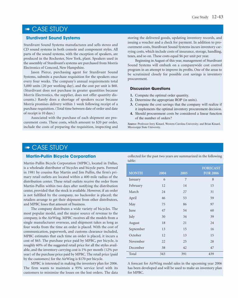
Case Study 12-43

➠ CASE STUDYSturdivant Sound Systems

Sturdivant Sound Systems manufactures and sells stereo andCD sound systems in both console and component styles. Allparts of the sound systems, with the exception of speakers, areproduced in the Rochester, New York, plant. Speakers used inthe assembly of Sturdivant’s systems are purchased from MorrisElectronics of Concord, New Hampshire.

Jason Pierce, purchasing agent for Sturdivant SoundSystems, submits a purchase requisition for the speakers onceevery four weeks. The company’s annual requirements total5,000 units (20 per working day), and the cost per unit is $60.(Sturdivant does not purchase in greater quantities becauseMorris Electronics, the supplier, does not offer quantity dis-counts.) Rarely does a shortage of speakers occur becauseMorris promises delivery within 1 week following receipt of apurchase requisition. (Total time between date of order and dateof receipt is 10 days.)

Associated with the purchase of each shipment are pro-curement costs. These costs, which amount to $20 per order,include the costs of preparing the requisition, inspecting and

storing the delivered goods, updating inventory records, andissuing a voucher and a check for payment. In addition to pro-curement costs, Sturdivant Sound Systems incurs inventory car-rying costs, which include costs of insurance, storage, handling,taxes, and so on. These costs equal $6 per unit per year.

Beginning in August of this year, management of SturdivantSound Systems will embark on a companywide cost control program in an attempt to improve its profits. One of the areas tobe scrutinized closely for possible cost savings is inventory procurement.

Discussion Questions

1. Compute the optimal order quantity.2. Determine the appropriate ROP (in units).3. Compute the cost savings that the company will realize if

it implements the optimal inventory procurement decision.4. Should procurement costs be considered a linear function

of the number of orders?

Source: Professor Jerry Kinard, Western Carolina University; and Brian Kinard,Mississippi State University.

➠ CASE STUDYMartin-Pullin Bicycle Corporation

Martin-Pullin Bicycle Corporation (MPBC), located in Dallas,is a wholesale distributor of bicycles and bicycle parts. Formedin 1981 by cousins Ray Martin and Jim Pullin, the firm’s pri-mary retail outlets are located within a 400-mile radius of thedistribution center. These retail outlets receive the order fromMartin-Pullin within two days after notifying the distributioncenter, provided that the stock is available. However, if an orderis not fulfilled by the company, no backorder is placed; theretailers arrange to get their shipment from other distributors,and MPBC loses that amount of business.

The company distributes a wide variety of bicycles. Themost popular model, and the major source of revenue to thecompany, is the AirWing. MPBC receives all the models from asingle manufacturer overseas, and shipment takes as long asfour weeks from the time an order is placed. With the cost ofcommunication, paperwork, and customs clearance included,MPBC estimates that each time an order is placed, it incurs acost of $65. The purchase price paid by MPBC, per bicycle, isroughly 60% of the suggested retail price for all the styles avail-able, and the inventory carrying cost is 1% per month (12% peryear) of the purchase price paid by MPBC. The retail price (paidby the customers) for the AirWing is $170 per bicycle.

MPBC is interested in making the inventory plan for 2006.The firm wants to maintain a 95% service level with its customers to minimize the losses on the lost orders. The data

collected for the past two years are summarized in the followingtable:

FORECAST MONTH 2004 2005 FOR 2006

January 6 7 8

February 12 14 15

March 24 27 31

April 46 53 59

May 75 86 97

June 47 54 60

July 30 34 39

August 18 21 24

September 13 15 16

October 12 13 15

November 22 25 28

December 38 42 47

Total 343 391 439

A forecast for AirWing model sales in the upcoming year 2006has been developed and will be used to make an inventory planfor MPBC.


Discussion Questions

1. Develop an inventory plan to help MPBC.2. Discuss ROPs and total costs.

3. How can you address demand that is not at the level of theplanning horizon?

Source: “Martin-Pullin Bicycle Corporation” by Professor Kala Chand Seal, LoyolaMarymount University. Copyright © Kala Chand Seal. Reprinted with permission.

INTERNET CASE STUDIES

See our Internet home page at www.prenhall.com/balakrishnan for theseadditional case studies:

� Professional Video Management� Drake Radio� La Place Power� Western Ranchman Outfitters

BIBLIOGRAPHYBangash, Alex, Ramesh Bollapragada, Rachelle Klein, Narayan Raman,

Herbert B. Shulman, and Donald R. Smith. “InventoryRequirements Planning at Lucent Technologies,” Interfaces 34, 5(September–October 2004): 342–352.

Bernard, Paul. “Are Your Customers Getting Better Service Than YouPlanned to Provide?” APICS—The Performance Advantage (July1997): 30–32.

Bowers, Melissa R., and Anurag Agarwal. “Lower In-Process Inventoriesand Better on-Time Performance at Tanner Companies, Inc.,”Interfaces 25, 4 (July–August 1995): 30–43.

Denton, D. Keith. “Top Management’s Role in Inventory Control,”Industrial Engineering (August 1994): 26–27.

Edds, Daniel. “The Real Costs of Quantity Discounts,” School Planningand Management (March 1998): 14.

Emmons, Hamilton, et al. “The Role of Return Policies in Pricing andInventory Decisions for Catalogue Goods,” Management Science(February 1998): 276–283.

Gould, Eppen, et al. “Backup Agreements in Fashion Buying,”Management Science (November 1997): 1469–1484.

Greis, Noel. “Assessing Service Level Targets in Production and InventoryPlanning,” Decision Sciences 25, 1 (January–February 1994): 15–40.

Kapuscinski, Roman., Rachel Q. Zhang, Paul Carbonneau, RobertMoore, and Bill Reeves. “Inventory Decisions in Dell’s SupplyChain,” Interfaces 34, 3 (May–June 2004): 191–205.

Katok, E., T. Serrander, and M. Wennstrom. “Setup Reduction throughProcess Improvement in Aluminum Can Manufacturing,”Production and Inventory Management Journal 29, 4 (fourth quarter1998): 77–82.

Landvater, D. V. World Class Production and Inventory Management.Newburg, NH: Oliver Wight Publications (1997).

Lieberman, M. B., S. Helper, and L. Demeester. “The EmpiricalDeterminants of Inventory Levels in High-Volume Manufacturing,”Production and Operations Management 1 (Spring 1999): 44–55.

Millet, Ido. “How to Find Inventory by Not Looking,” Interfaces (March1994): 69–75.

Sandvig, J. C. “Calculating Safety Stock,” IIE Solutions 30, 12 (December1998): 28–29.

Smock, Doug. “Games Tip the Scale at Milton Bradley,” Plastics World(March 1997): 22–26.

Sox, Charles, et al. “Coordinating Production and Inventory to ImproveService,” Management Science (September 1997): 1189–1197.

van der Duyn Schouten, Frank, et al. “The Value of Supplier Informationto Improve Management of a Retailer’s Inventory,” Decision Sciences25, 1 (January–February 1994): 1–14.

inventory control models - Canvas

Documents

Transcript of inventory control models - Canvas