Notes on Price Theory - UChicago Canvas
187
Notes on Price Theory Scott Ashworth September 16, 2018
-
Upload
khangminh22 -
Category
Documents
-
view
2 -
download
0
Transcript of Notes on Price Theory - UChicago Canvas

Notes on Price Theory
Scott Ashworth
September 16, 2018

Contents
I Foundations 6
1 Rational Choice Theory 7
1.1 The Standard Approach . . . . . . . . . . . . . . . . . . . . . . . . . . . . . 8
1.2 Problems and Alternatives . . . . . . . . . . . . . . . . . . . . . . . . . . . . 13
2 Optimization and Concavity 19
2.1 How to Think About Derivatives . . . . . . . . . . . . . . . . . . . . . . . . 19
2.2 Optimization Problems . . . . . . . . . . . . . . . . . . . . . . . . . . . . . . 20
2.2.1 Necessary Conditions . . . . . . . . . . . . . . . . . . . . . . . . . . 21
2.3 Concave Optimization . . . . . . . . . . . . . . . . . . . . . . . . . . . . . . 22
2.3.1 The Kuhn-Tucker Theorem . . . . . . . . . . . . . . . . . . . . . . . 24
II Core Price Theory 27
3 Choice Under Uncertainty 28
3.1 Expected Utility . . . . . . . . . . . . . . . . . . . . . . . . . . . . . . . . . 29
3.2 Difficulties and Extentions . . . . . . . . . . . . . . . . . . . . . . . . . . . . 33
3.3 Utility for Money . . . . . . . . . . . . . . . . . . . . . . . . . . . . . . . . . 35
3.3.1 Risk Aversion . . . . . . . . . . . . . . . . . . . . . . . . . . . . . . . 35
3.3.2 Comparing Risk Aversion . . . . . . . . . . . . . . . . . . . . . . . . 37
3.3.3 Stochastic Dominance . . . . . . . . . . . . . . . . . . . . . . . . . . 44
4 Consumer Theory: A First Look 52
4.1 The Setting . . . . . . . . . . . . . . . . . . . . . . . . . . . . . . . . . . . . 52
4.1.1 Consumer Preferences . . . . . . . . . . . . . . . . . . . . . . . . . . 52
4.1.2 The Consumer’s Problem . . . . . . . . . . . . . . . . . . . . . . . . 54
1

CONTENTS 2
4.2 Solving the Consumer’s Problem . . . . . . . . . . . . . . . . . . . . . . . . 55
4.3 Empirical Implications of CP . . . . . . . . . . . . . . . . . . . . . . . . . . 61
4.3.1 Empirical Applications . . . . . . . . . . . . . . . . . . . . . . . . . . 63
4.3.2 Downward-Sloping Demand? . . . . . . . . . . . . . . . . . . . . . . 65
4.3.3 Aggregating Demand . . . . . . . . . . . . . . . . . . . . . . . . . . . 67
5 Production 71
5.1 Technology . . . . . . . . . . . . . . . . . . . . . . . . . . . . . . . . . . . . 72
5.2 Profit Maximization . . . . . . . . . . . . . . . . . . . . . . . . . . . . . . . 74
5.3 Aggregate Production . . . . . . . . . . . . . . . . . . . . . . . . . . . . . . 77
5.4 Prices from Efficiency . . . . . . . . . . . . . . . . . . . . . . . . . . . . . . 79
5.5 Decentralization via Prices . . . . . . . . . . . . . . . . . . . . . . . . . . . . 83
5.6 Appendix: Subjective Probability . . . . . . . . . . . . . . . . . . . . . . . . 86
6 Welfare Economics 92
6.1 Normative Concepts for Welfare Economics . . . . . . . . . . . . . . . . . . 93
6.2 Characterizing Efficient Allocations . . . . . . . . . . . . . . . . . . . . . . . 97
6.2.1 Bergen-Samuleson Social Welfare Functionals . . . . . . . . . . . . . 97
6.2.2 Efficient Allocations of Commodities . . . . . . . . . . . . . . . . . . 98
6.3 Further Directions . . . . . . . . . . . . . . . . . . . . . . . . . . . . . . . . 100
6.3.1 Arrow’s Impossibility Theorem . . . . . . . . . . . . . . . . . . . . . 100
6.3.2 Prices and Walrasian Equilibrium . . . . . . . . . . . . . . . . . . . 103
6.3.3 Towards Cost-Benefit Analysis . . . . . . . . . . . . . . . . . . . . . 106
6.4 Appendix: Technical Details . . . . . . . . . . . . . . . . . . . . . . . . . . . 108
6.4.1 Proof of Arrow’s Theorem . . . . . . . . . . . . . . . . . . . . . . . . 108
6.4.2 Existence and Uniqueness of Walrasian Equilibrium . . . . . . . . . 109
7 The Envelope Theorem 114
7.1 A Formal Statement and Application . . . . . . . . . . . . . . . . . . . . . . 117
7.1.1 Cost Minimization . . . . . . . . . . . . . . . . . . . . . . . . . . . . 119
7.2 Some Formal Details and Extentions . . . . . . . . . . . . . . . . . . . . . . 121
7.2.1 The Second-Price Auction . . . . . . . . . . . . . . . . . . . . . . . . 123
III Specialty Topics 126
8 Consumer Theory: A Deeper Look 127

CONTENTS 3
8.1 Duality in Consumer Theory . . . . . . . . . . . . . . . . . . . . . . . . . . 127
8.2 Comparative Statics of Compensated Demand . . . . . . . . . . . . . . . . . 131
8.3 Welfare Measures . . . . . . . . . . . . . . . . . . . . . . . . . . . . . . . . . 135
9 The Second Best 140
9.1 First-Best: Price Regulation . . . . . . . . . . . . . . . . . . . . . . . . . . . 140
9.2 The Second-Best: Ramsey Pricing . . . . . . . . . . . . . . . . . . . . . . . 143
9.3 Two More Applications . . . . . . . . . . . . . . . . . . . . . . . . . . . . . 145
9.3.1 An Ineliminable Distortion . . . . . . . . . . . . . . . . . . . . . . . 145
9.3.2 Equity and Efficiency . . . . . . . . . . . . . . . . . . . . . . . . . . 146
10 Monotone Comparative Statics 149
10.1 Comparative Statics of the Firm: The Traditional Approach . . . . . . . . . 149
10.2 The Main Theorems . . . . . . . . . . . . . . . . . . . . . . . . . . . . . . . 151
10.2.1 The Method of Aggregation . . . . . . . . . . . . . . . . . . . . . . . 155
10.2.2 Supermodularity . . . . . . . . . . . . . . . . . . . . . . . . . . . . . 156
10.2.3 Proof of Theorem 10.3 . . . . . . . . . . . . . . . . . . . . . . . . . . 158
10.3 Applications of Complementarity . . . . . . . . . . . . . . . . . . . . . . . . 161
10.3.1 Short-run vs. Long-run Responses . . . . . . . . . . . . . . . . . . . 161
10.3.2 The Firm as an Incentive System . . . . . . . . . . . . . . . . . . . . 162
IV Advanced Topics 166
11 Topics in Uncertainty and Information 167
11.1 Risk-Bearing and Moral Hazard . . . . . . . . . . . . . . . . . . . . . . . . . 167
12 Dynamic Choice 174
12.1 Intertemporal Consumer Theory . . . . . . . . . . . . . . . . . . . . . . . . 175
12.2 Dynamic Programming . . . . . . . . . . . . . . . . . . . . . . . . . . . . . 180

Motivating Example
How will a person change the number of hours she works in response to a change in taxes
and transfer payments?
Ask an economist a question like this, and she will automatically think in terms of
models. She might, for example, offer the following analysis:
Consider an agent endowed with 24 hours of time who can earn a wage of
w per hour of work. The government takes a fraction τ of her labor income in
taxes, and also pays her a fixed transfer T ≥ 0. She spends her post-tax-and-
transfer income on a single consumption good. So, if she works ` hours, she can
consume any amount c with c ≤ (1− τ)w`+ T .
The agent chooses hours ` and consumption c to maximize a function u(c, `).
For concreteness, let’s take u(c, `) = log(c) + log(24− `). The choices solve:
maxc,`
log(c) + log(24− `)
st c ≤ (1− τ)w`+ T.
Since u is strictly increasing in c, we know that the inequality in the constraint
will hold with equality. Thus we can substitute into the maximand to get:
max`
log ((1− τ)w`+ T ) + log(24− `).
The solution depends on the parameters (w, τ, T ):
`∗(w, τ, T ) and c∗(w, τ, T ).
Being able to solve problems like this on your own is the most essential prerequisite for
this course. Give it a shot before turning the page.
4

CONTENTS 5
I hope you found:
`∗(w, τ, T ) = 12− T
2(1− τ)wand c∗(w, τ, T ) = 12(1− τ)w +
1
2T.
Now, back to our economist’s answer:
Increased transfer payments lead to fewer hours worked, since ∂`∗
∂T < 0. If
transfers are strictly positive, then a higher tax rate leads to fewer hours worked,
since ∂`∗
∂τ < 0 in that case. But if transfers are 0, then the tax rate has no effect
on hours worked.
Maybe you wanted to know about hours worked out of simple curiosity. But maybe
not. Maybe your question was motivated by the hope that the answer would help you know
what tax rate would be best. Our economist can help there as well.
She will define a new function v by:
v(w, τ, T ) = u(c∗(w, τ, T ), `∗(w, τ, T )).
And then she use this new function as a part of another maximization problem, one in
which the choice variables include the tax and transfer.
All of this should raise several questions in your mind.
1. Why model the worker’s decisions as the result of maximizing some function?
2. Granting that we should model decisions that way, why should the value of that
function play a role in policy decisions?
3. How sensitive are the conclusions to the specific functional form we chose for u?
4. If they are sensitive, can we get useful conclusions with weaker assumptions?
Answering questions like these is the major goal of this course. Not surprisingly, this
will involve doing a lot of math. On the one hand, we will make extensive use of the
mathematical theory of optimization, using techniques both for characterizing solutions
and for exploring how solutions change as parameters of the problem change. On the other
hand, we will use the axiomatic method to explore how optimization problems are related
to more intuitively acceptable descriptions of the problems that face economic agents. By
doing both, we will pursue an important subsidiary goal, to show how all of the calculus we
do while practicing economics can be interpreted in terms of human agency.

Part I
Foundations
6

Chapter 1
Rational Choice Theory
We want to consider a decision maker (DM for short) who chooses “rationally”. The
standard approach to modeling rational choice can be presented three ways:
1. DM chooses an alternative that is best according to a binary relation %, with the
interpretation “a % b if and only if DM likes a at least as much as b”.
2. DM chooses an alternative that maximizes a function u, called the utility function.
3. DM chooses according to some choice rule that satisfies a consistency assumption
across different choice problems.
And we standardly impose assumptions on preference relations and choice rules that render
all three approaches equivalent.
But they are not equivalent in terms of how we think about them. Utility maximization
feels like a strange assumption, but is easy (relatively!) to work with. Consistent choice is
just the opposite. And that’s the value of having three different representations.
Here is how I think of the relationships of the three approaches.
We all have an intuitive account of human action—philosophers call it “folk psychology”.
A corner-stone is a claim like:
People usually act to, more or less, satisfy their preferences, in light of their
beliefs.
Decision theory formalizes an idealized version of this:
People usually act to, more or less, satisfy their preferences, in light of their
beliefs.
Beliefs will be mostly in the background until we talk about uncertainty explicitly.
7

CHAPTER 1. RATIONAL CHOICE THEORY 8
1.1 The Standard Approach
The formalization starts with a decision maker and a set of alternatives A. DM has pref-
erences described by a binary relation %, with the interpretation that a % b means DM
weakly prefers a to b. From %, we can derive two other relations on A:
1. The strict preference relation,
a b ⇐⇒ a % b but not b % a
interpreted as “DM likes a better than b.”
2. The indifference relation, ∼
a ∼ b ⇐⇒ a % b and b % a
interpreted as “DM is indifferent between a and b.”
Now for the big assumptions. A preference relation is rational if satisfies two axioms
1. Completeness: For all a, b ∈ A, a % b or b % a (or both)
2. Transitivity: For all a, b, c ∈ A, if a % b and b % c, then a % c.
A choice problem is a nonempty subset B ⊂ A of alternatives that the DM believes to
be feasible. The preference maximizing choices are:
C∗ (B,%) = a ∈ B | a % b, for all b ∈ B
In words, C∗ takes the elements of B and returns the subset that are most-preferred by DM.
If C∗(B,%) is a singleton, then we assume DM chooses the single element. If it contains
multiple elements the DM is indifferent among them, but prefers all elements of C∗ to
any other element of B. In this case, we assume only that DM chooses some element of
C∗(B,%).
So we see that rational choice theory has two parts: choices are made to (1) maximize
a (2) rational preference relation.
The advantage of this approach is that the axioms are clear and easy to think about.
Specifically, we can see how strong they are. For example, completeness means DM can
always express a preference between two elements (even if that preference is indifference).
DM is not permitted to say, “I don’t know how to compare these things.” That is, DM has
CHAPTER 1. RATIONAL CHOICE THEORY 9
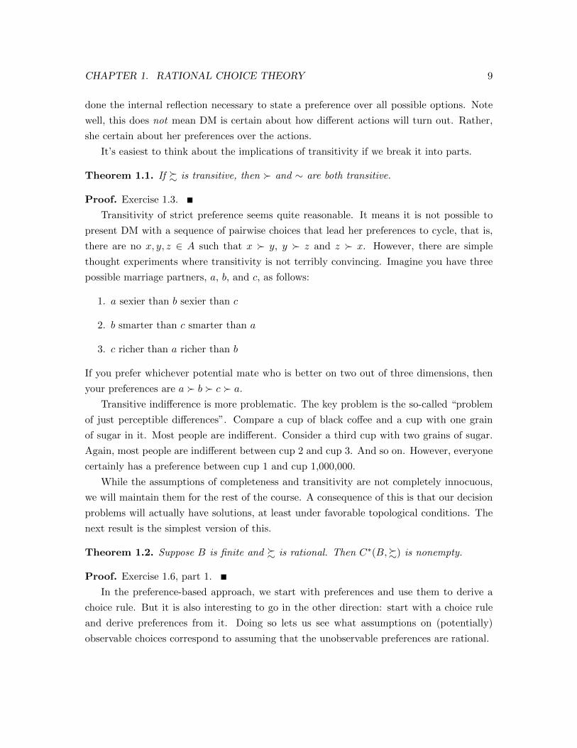
done the internal reflection necessary to state a preference over all possible options. Note
well, this does not mean DM is certain about how different actions will turn out. Rather,
she certain about her preferences over the actions.
It’s easiest to think about the implications of transitivity if we break it into parts.
Theorem 1.1. If % is transitive, then and ∼ are both transitive.
Proof. Exercise 1.3.
Transitivity of strict preference seems quite reasonable. It means it is not possible to
present DM with a sequence of pairwise choices that lead her preferences to cycle, that is,
there are no x, y, z ∈ A such that x y, y z and z x. However, there are simple
thought experiments where transitivity is not terribly convincing. Imagine you have three
possible marriage partners, a, b, and c, as follows:
1. a sexier than b sexier than c
2. b smarter than c smarter than a
3. c richer than a richer than b
If you prefer whichever potential mate who is better on two out of three dimensions, then
your preferences are a b c a.
Transitive indifference is more problematic. The key problem is the so-called “problem
of just perceptible differences”. Compare a cup of black coffee and a cup with one grain
of sugar in it. Most people are indifferent. Consider a third cup with two grains of sugar.
Again, most people are indifferent between cup 2 and cup 3. And so on. However, everyone
certainly has a preference between cup 1 and cup 1,000,000.
While the assumptions of completeness and transitivity are not completely innocuous,
we will maintain them for the rest of the course. A consequence of this is that our decision
problems will actually have solutions, at least under favorable topological conditions. The
next result is the simplest version of this.
Theorem 1.2. Suppose B is finite and % is rational. Then C∗(B,%) is nonempty.
Proof. Exercise 1.6, part 1.
In the preference-based approach, we start with preferences and use them to derive a
choice rule. But it is also interesting to go in the other direction: start with a choice rule
and derive preferences from it. Doing so lets us see what assumptions on (potentially)
observable choices correspond to assuming that the unobservable preferences are rational.

CHAPTER 1. RATIONAL CHOICE THEORY 10
The basic story is this: choices make up the preference maximizing choice rule for some
rational preference if and only if those choices satisfy cross-decision-problem consistency
conditions. Rubinstein handles the general case; here we will focus on a simple version.
First, we restrict attention to choice rules that always specify a unique alternative. (Such
rules are said to be resolute.) Write B for the set of all non-empty subsets of A. Then a
resolute choice rule is a function C : B → A such that C(B) ∈ B for all B ∈ B.
A resolute choice rule C is contraction consistent if, whenever B and D are subsets
with D ⊂ B, we have C(B) ∈ D implies C(B) = C(D). Intuitively, removing unchosen
alternatives does not affect the choice.
The next result shows the first part of a kind of equivalence between the preference-
based approach and the choice function-based approach. (Exercise 1.7 asks you to show
the second part of the equivalence.) Say that a choice function, C, and the choice function
derived from preferences %, C∗(·,%), agree for finite B if C(B) = C∗(B,%) whenever
B ⊂ A has only finitely many elements. (Note: this does not presuppose that A is finite.)
Theorem 1.3. Suppose C is a contraction consistent, resolute choice rule. Then there is
a rational preference %C such that C and C∗(·,%C) agree for finite B.
Proof. The first step is to come up with the preference relation. Define a %C b if
C(a, b) = a.
Next, we show that this preference is rational. C(a, b) is either a or b. In the first
case, we have a %C b. In the second, we have b %C a. Since at least one obtains, %C is
complete.
Next we show that this preference is transitive. Suppose x %C y and y %C z. From
the definition, this means C(x, y) = x and C(y, z) = y. Consider C(x, y, z). It
can’t be y, because if it were, contraction consistency would force C(x, y) = y. And it
can’t be z, because if it were, contraction consistency would force C(y, z) = z. Thus
C(x, y, z) = x. But then contraction consistency gives C(x, z) = x, and that implies
x %C z.
Finally, we show that C = C∗(·,%C). We argue by contradiction: suppose there is a
finite subset B such that C(B) 6= C∗(B,%C). By Theorem 1.2, this means that C(B) = x
and C∗(B,%C) contains some y 6= x. The second of these implies y %C x, but the first and
contraction consistency imply C(x, y) = x, contradicting the definition of %C .
The preference relation defined in the proof, %C , is an example of a revealed preference.
This idea will come back in Section 4.3, where is will even be related directly to empirical
work.

CHAPTER 1. RATIONAL CHOICE THEORY 11
The last result linked preferences (which are good for thinking) and choices (which
are good for observing). The next one relates preferences to utility (which is good for
calculating).
A function u : A → R represents % if, for every a, b ∈ A, u(a) ≥ u(b) if and only
if a % b. Such a function is sometimes called a utility function. It assigns a numerical
value to each element in A, ranking them numerically in accordance with the individual’s
preferences. This is useful because maximizing a real-valued function is an easy way to
determine most preferred elements of A.
Utility functions that represent a preference relation % are not unique—any strictly
increasing transformation still represents same preference relation. Formally, consider any
strictly increasing function f : R → R. Then v (x) = f (u (x)) is new utility function
representing the same preferences as u (·). To see this, note that
v (a) ≥ v (b)
⇔ f(u(a)) ≥ f(u(b))
⇔ u (a) ≥ u (b) .
Properties of utility functions that are invariant to any strictly increasing transformation
are called ordinal. The ordinal properties are exactly the ones that are meaningful in
terms of preferences. Properties that are not ordinal include magnitude (or intensity) of
preference—there is no difference between the comparison of 100 to 0 and the comparison of
1 to 0. This is very different from the classical utilitarian concept of utility from Bentham
and Mill.
Theorem 1.4. Suppose % is represented by the function u. Then % is rational
Proof. Exercise 1.4.
To further developing the formal relationship between preferences and utility, we need
a technical result. Say that an element a ∈ X is %-minimal in X if x % a for all x ∈ X.
Lemma 1.1. Suppose A is finite and % is rational. Then every non-empty subset X ⊂ A
has a %-minimal element.
Proof. We proceed by induction on the number of elements of X. If X has a single element,
then the claim follows from completeness. So assume that the claim is true for any X ′ with
n elements, and let X have n + 1 elements. Choose an arbitrary x ∈ X, and consider the
set X ′ = X \ x. This set has n elements, so the inductive hypothesis tells us that it has
a %-minimal element—call it y. By completeness, we have either x % y or y % x. In the

CHAPTER 1. RATIONAL CHOICE THEORY 12
first case, y is %-minimal in X. In the second case, transitivity implies x is %-minimal in
X. Either way, X has a %-minimal element.
Theorem 1.5. Suppose A is finite. A preference relation, %, can be represented by a utility
function if % is rational.
Proof. We start by iteratively constructing subsets of A. Let X1 be the set of %-minimal
elements of A. This is non-empty by Lemma 1.1. Now assume we have constructed sets
X1, . . . , Xk. If X1∪· · ·∪Xk = A, then we are done. Otherwise, the set A\ (X1∪· · ·∪Xk) is
non-empty, and by the Lemma, has a %-minimal element. Let Xk+1 be the set of all these
%-minimal elements. Notice that this construction will stop after at most n steps, where n
is the number of elements of A.
Define u(x) = k if x ∈ Xk. I claim that u represents %. To see this, consider a b.
Transitivity implies a 6∈ X1 ∪ · · · ∪ Xu(b). Thus u(a) > u(b). And if a ∼ b, then a is
%-minimal if and only if b is, so u(a) = u(b).
You’ll notice that our result on the existence of a utility representation required A to be
finite. This is disappointing, since in applications we want to use calculus, which doesn’t
even make sense on finite A. But we really do need to go beyond just rationality to handle
all of the A that we would like.
For an example of what can go wrong, let A = [0, 1] × [0, 1]. The lexicographic
preference on A is defined as follows:
(x1, x2) % (y1, y2)⇔
x1 > y1
or
x1 = y1 and x2 ≥ y2
You can verify that these preferences are rational. But:
Proposition 1.1. There does not exist any utility representation of lexicographic prefer-
ences.
Proof. We will use two facts from mathematics:
1. If x and y are any real numbers with x > y, then there is a rational number q with
x > q > y.
2. There does not exist any function f from [0, 1] to the rational numbers such that
x 6= y implies f(x) 6= f(y).

CHAPTER 1. RATIONAL CHOICE THEORY 13
The proof of the proposition is by contradiction: we assume there is a utility represen-
tation and use it along with fact 1 to construct a function q : [0, 1] → Q such that x 6= y
implies q(x) 6= q(y). Since fact 2 says that is impossible, we know that there cannot be a
utility representation after all.
Now for the details. Suppose u is a utility representation of lexicographic preferences.
For every x ∈ [0, 1], we have u(x, 1) > u(x, 0). Fact 1 tells us there is a rational number
q(x) such that u(x, 1) > q(x) > u(x, 0). If x > y, we have
q(x) > u(x, 0) > u(y, 1) > q(y),
so q(x) 6= q(y).
Preferences are continuous if, for any sequences of bundles xn → x and yn → y, if
xn % yn for all n, then x % y. A useful way to see what this means is to see that it rules out
lexicographic preferences. Consider the bundle x = (0, 1) and the sequence (yn) = (1/n, 0).
For every n, we have yn x, because 1/n > 0. But the sequence has limit y = (0, 0), and
x y. In this case, the preference switched from strict one way to strict the other way
without ever passing through indifference along the way. Continuity rules that out.
This is just what we need to get a utility representation.
Theorem 1.6 (Debreu). Preferences are complete, transitive, and continuous if and only
if they are represented by a continuous utility function.
1.2 Problems and Alternatives
The standard approach to preferences, choices, and utility has been extremely fruitful for
economics and other social sciences. But not everything that we might want to model can
be captured in the standard framework.
Here is an example, from an experiment conducted by Kahneman and Tversky. In one
arm of the experiment, subjects were told:
Imagine that the U.S. is preparing for the outbreak of an unusual Asian dis-
ease, which is expected to kill 600 people. Two alternative programs to combat
the disease have been proposed. Assume that the exact scientific estimate of
the consequence of the program are as follows:
• If program A is adopted, 200 people will be saved.
• If program B is adopted, there is 2/3 probability that no one will be saved,
and 1/3 probability that 600 people will be saved.

CHAPTER 1. RATIONAL CHOICE THEORY 14
72% of subjects reported that program A was best.
In the second arm, subjects were told:
Imagine that the U.S. is preparing for the outbreak of an unusual Asian dis-
ease, which is expected to kill 600 people. Two alternative programs to combat
the disease have been proposed. Assume that the exact scientific estimate of
the consequence of the program are as follows:
• If program C is adopted, 400 people will die with certainty.
• If program D is adopted, there is 2/3 probability that 600 people will die,
and 1/3 probability that no one will die.
78% of subjects reported that program D was best.
Why is this a problem for the standard approach? Well, A and C are the same program,
as are B and D. So the experimental results say that identical alternatives will be treated
differently depending on how they are described. (Kahneman and Tversky call this a
framing effect.) The problem for the standard approach is that that approach ignores
descriptions altogether.
Psychologists are good at cooking up experiments like this to falsify just about any
assumption you might want to make about decision making. Opinions are divided about
how to respond. One camp holds that the deviations from the standard approach are not a
big deal, and the standard approach is a good approximation for applications in the social
sciences. Another camp holds that the deviations are important for applications, and that
we need improved models that can accommodate them. Much recent work in behavioral
economics has tried to assess the importance of deviations in field, rather than lab, data.
The standard approach can be called into question by thought experiments just as much
as by actual experiments. Suppose a choice function defined on x, y, z fails contraction
consistency:
C(x, y, z) = x but C(x, y) = y.
Before you declare this choice function irrational, two people speak up.
Ann says:
That is my choice function, and it is rational. The alternatives are x = duck,
y = chicken, and z = frog legs. I prefer duck to chicken exactly when the chef
is well trained. And I learn about the quality of the chef from the menu. If she
cooks frog legs, she is probably well trained. But if she doesn’t, I’d rather be
safe and order chicken.

CHAPTER 1. RATIONAL CHOICE THEORY 15
Ann learns information relevant to her decision from the feasible set.
Bob says:
That is my choice function, and it is rational. The alternatives are cookies:
x = chocolate-chip, y = oatmeal-raisin, and z = peanut-butter. My parents
taught me that it’s rude to take the best desert when others have to choose
latter, so I always choose my second favorite.
Bob has a complete and transitive order on alternatives, but chooses the second best from
any feasible set.
These examples suggest allowing preferences to depend on the feasible set, or even on
the way it is described. But we don’t want to go too far with this—we still want to say
that some observations are ruled out by the model. Coming up with disciplined ways to
incorporate choice-set dependence into preferences is an active area of current research.
Here, we’ll just look quickly at one approach.
The model we are about to develop is motivated by empirical evidence that default
options often influence choices. One example comes from Sweden’s public pension reform,
passed in 1998. One provision of the plan was that, from 2000 on, proceeds of a 2.5% payroll
tax were put into individual investment accounts. Individual could choose up to five funds
from an approved list. There was close to free entry to the list, and there were 456 funds
available at the start. One was a default fund for those who made no choice. At the start
of the plan, against the background of extensive advertising campaign to promote choice of
funds, 33.1% of investors allocated to the default. By 2003, 91.6% of new entrants allocated
to the default. Experiences like this have made setting defaults an important part of policy
design in the “nudge” approach to policy reform.
Here is a model that gives a role to defaults.1 As before, A is the set of alternatives.
But now, a choice problem is a pair (B, d), where B ⊆ A is the feasible set and d ∈ B is the
default. The decision maker is characterized by two functions. The first is a utility function
u : A → R that represents DM’s “true” preferences. The second function, b : A → R+,
gives a bonus to the default.
For simplicity assume that x 6= y implies u(x) 6= u(y). Choices are given by the function
Cu,b(B, d) =
d if u(d) + b(d) ≥ u(x) for all x 6= d
x if u(x) > u(d) + b(d) and u(x) > u(y) for all y 6= x, d
For an example, take A = x, y, with the functions u(x) = 1, u(y) = 0 and b(x) =
1This model is from chapter 3 of Rubinstein.

CHAPTER 1. RATIONAL CHOICE THEORY 16
b(y) = 2. Then Cu,b(A, x) = x but Cu,b(A, y) = y. Thus choices are sensitive to the default,
as we intended.
And the model does restrict how choices change across decision problems. Let B and D
be feasible sets with d ∈ D ⊂ B, and suppose Cu,b(B, d) ∈ D. There are two possibilities:
1. Cu,b(B, d) = d.
The definition of Cu,b tells us that u(d) + b(d) > u(x) for all x ∈ B with x 6= d. Since
x ∈ D implies x ∈ B, this means u(d) + b(d) > u(x) for all x ∈ D with x 6= d, and
Cu,b(D, d) = d.
2. Cu,b(B, d) = x 6= d.
The definition of Cu,b tells us that there is an x with u(x) > u(d)+b(d) and u(x) > u(y)
for all y ∈ B other than x and d. Since x ∈ D implies x ∈ B, this means u(x) >
u(d) + b(d) and u(x) > u(y) for all y ∈ B other than x and d, and Cu,b(D, d) = x.
Thus Cu,b satisfies a restricted version of contraction consistency.
This is far from the last word on the subject of choice-set dependence, but it is enough to
illustrate that the phenomenon can be captured in a model that both builds on the decision
theoretic tradition and has enough bite to avoid vacuousness.
The strategy for the next four chapters is this. We will apply the standard approach
of decision theory to specific decision-making environments: choice under uncertainty, con-
sumer choice in markets, choice of production plans, and normatively good choice by a
policy maker. In each case, we will exploit the special structure of the applied problem to
motivate assumptions about preferences, show how those assumptions on preferences give
useful special structure to utility functions, and use that structure to learn about choices.
Exercises
Exercise 1.1. Consider a DM with preferences
a ∼ b c d e ∼ f.
1. What is C∗(a, b, c,%)?
2. What is C∗(d, e, f,%)?

CHAPTER 1. RATIONAL CHOICE THEORY 17
3. Construct two different utility representations for these preferences.
Exercise 1.2. Kahneman and Tversky (1984) asked experimental subjects to consider the
three following choice problems.
You are about to buy a stereo for $125 and a calculator for $15.
You learn there is a $5 calculator discount at another store branch, ten minutes
away. Do you make the trip?
You learn there is a $5 stereo discount at another store branch, ten minutes
away. Do you make the trip?
You learn both items are out of stock. You must go to the other branch, but as
compensation you will get a $5 discount. Do you care which item is discounted?
1. What are your answers?
2. Most people answer yes to the first question, no to the second question, and are
indifferent in the third case. Let x be traveling to the other store and getting a
calculator discount, y be traveling to the other store and getting a stereo discount,
and z be staying at the first store. Are the usual preferences over x, y, z rational?
Exercise 1.3. Prove Theorem 1.1.
Exercise 1.4. Prove Theorem 1.4.
Exercise 1.5. Consider two people. Let %1 be 1’s (complete and transitive) preferences
on a finite set A, and let %2 be 2’s. For their “joint” preference %∗they define
x %∗ y if x %1 y and x %2 y
In words, as a pair they weakly prefer x to y if both of them weakly prefer x to y. Prove
that %∗ is transitive. Show by example that it need not be complete.
Exercise 1.6. We saw that infinite A can cause problems for the existence of a utility
representation of rational preferences. Infinite A can also cause problems for C∗.
1. Suppose A is finite and % is complete and transitive. Show that C∗(B,%) is nonempty
for all B ⊆ A. (Hint: Mimic the argument from Lemma 1.1.)
2. Let A = [0, 1] and define % by x % y if and only if x ≥ y. Find a subset B ⊂ A such
that C∗(B,%) is empty.

CHAPTER 1. RATIONAL CHOICE THEORY 18
Exercise 1.7. This exercise will provide a converse to Theorem 1.3. To avoid the problem
pointed out in the previous exercise, assume throughout that A is finite.
Suppose % is complete and transitive, and that there is no pair x 6= y with x ∼ y.
1. Show that C∗(·,%) is resolute.
2. Show that C∗(·,%) is contraction consistent.

Chapter 2
Optimization and Concavity
2.1 How to Think About Derivatives
In calculus, you learned the following definition of the derivative. Let f : R → R, and let
x0 ∈ R. If the limit
limh→0
f(x0 + h)− f(x0)
h
exists and is a finite number L, then the derivative of f at x0 is f ′(x0) = L.
A slightly different way of thinking about this yields more insight into the generalization
to multiple dimensions. If the limit above is equal to L, then the function given by
η(h) =f(x0 + h)− f(x0)
h− L (2.1)
satisfies limh→0 η(h) = 0. Rearrange Equation 2.1 to get
f(x0 + h) = f(x0) + L · h+ η(h) · h.
This motivates a different definition of the derivative. If there is a number L and a
function η : R→ R such that limh→0 η(h) = 0 and, for all h,
f(x0 + h) = f(x0) + L · h+ η(h) · h,
then L is the derivative of f at x0, denoted f ′(x0).
Taking x = x0 +h, this reformulation says that, near x0, the function f is well approxi-
mated by the affine function x 7→ f(x0)+f ′(x0) ·(x−x0). The sense of “well-approximated”
19

CHAPTER 2. OPTIMIZATION AND CONCAVITY 20
is that the approximation error, (x− x0)η(x− x0) goes to 0 “faster than” x− x0.
This idea of approximation by affine maps is just what we need to generalize to higher
dimensions. A function f : Rn → R is differentiable at x0 if there is a linear map L : Rn → Rand a function η : Rn → R such that lim‖h‖→0 η(h) = 0 and, for all h,
f(x0 + h) = f(x0) + L(h) + ‖h‖η(h).
In a slight abuse of notation, we write Df(x0) both for the linear map L and for its
matrix representation with respect to the standard basis of Rn. This matrix turns out to
be in terms of the partial derivatives you studied in calculus:
Df(x0) =
∂f∂x1
(x0)...
∂f∂xn
(x0)
.
This way of thinking about derivatives provides the best way to understand the role of
derivatives in optimization.
2.2 Optimization Problems
We are now going to spend some time studying optimization problems of the form
maxx
f(x) (2.2)
st x ∈ X. (2.3)
Here, f is a function from some domain D ⊂ Rn+ to R, and X ⊂ D. f is the objective
function and X is the feasible set.
We typically describe X in terms of functions: for m functions hi : D → R, write
X = x ∈ D | hi(x) ≥ 0 ∀i.
Stack the constraint functions to simplify this to
X = x ∈ D | h(x) ≥ 0.
Theorem 2.1 (Extreme Value Theorem). If f is continuous and X is closed and bounded,
then the problem 2.2 has a solution.

CHAPTER 2. OPTIMIZATION AND CONCAVITY 21
(Outside of Rn, that X is closed and bounded is not sufficient. The more general notion
is compactness. In Rn, compactness is equivalent to being closed and bounded.)
Note that X will be closed if h is continuous.
For some purposes, this is all we need. But many important applications require a
characterization of the solution. And that is easiest if we have differentiability.
2.2.1 Necessary Conditions
Consider the problem:
maxx
f(x)
st x ∈ X ⊂ Rn
If x0 is a point in the interior of X where Df(x0) 6= 0, then x0 cannot be the solution to
the optimization problem. To see this, let k be the least index for which ∂f∂xk
(x0) 6= 0 and
let ek be the unit vector in the kth direction. At x = x0 + εek, we have
f(x) = f(x0) + ε∂f
∂xk(x0) + |ε|η(ε).
If ∂f∂xk
(x0) > 0, we can choose ε positive and small enough that ∂f∂xk
(x0) > η(ε), in which
case f(x) > f(x0). Similarly, if ∂f∂xk
(x0) < 0, we can choose ε < 0 negative and small enough
in absolute value that∣∣∣ ∂f∂xk (x0)
∣∣∣ > η(ε), in which case again f(x) > f(x0). Thus a necessary
condition for interior x0 to maximize f is that Df(x0) = 0.
A similar argument works when x0 is on the boundary of X, but it gives a bit less. For
now, we’ll focus on the case where X = Rn+; a more general case will come latter.
Suppose x0 is a boundary point. If ∂f∂xk
(x0) 6= 0 and xk > 0, the preceding argument
works without change. But if xk = 0, only the part with ε > 0 is valid. So we get the
weaker condition that ∂f∂xk
(x0) ≤ 0.
We have proved:
Theorem 2.2. Suppose that f is differentiable and x0 solves
maxx
f(x)
st x ∈ Rn+.
Then Df(x0) ≤ 0 and Df(x0) · x0 = 0.

CHAPTER 2. OPTIMIZATION AND CONCAVITY 22
Remark 2.1. I’m using the following conventions on vector inequalities:
• x ≥ y if xi ≥ yi for all i;
• x > y if x ≥ y and xi > yi for some i; and
• x y if xi > yi for all i.
2.3 Concave Optimization
It is rare that we just need a necessary condition of maximization. Sufficient conditions
involve assuming more about both X and f .
A subset X ⊂ Rn is convex if, whenever x and y are in X, and λ ∈ [0, 1], we have
λx + (1 − λ)y ∈ X. The function f : X → R is concave if λ ∈ [0, 1] implies that
f (λx+ (1− λ)y) ≥ λf(x) + (1 − λ)f(y). It is strictly concave if the inequality is strict
for all λ ∈ (0, 1). If f is differentiable, we have a particularly useful equivalent condition:
Theorem 2.3. Let f be differentiable. Then f is concave if and only if
f(y) ≤ f(x) + Df(x) · (y − x),
and f is strictly concave if and only if
f(y) < f(x) + Df(x) · (y − x).
This Theorem makes it easy to establish sufficient conditions for maximization.
Theorem 2.4. Suppose X is convex and f is differentiable and concave. Then x0 solves
maxx
f(x)
st x ∈ Rn+
if and only if Df(x0) ≤ 0 and Df(x0) · x0 = 0.
Proof. Theorem 2.2 established the “only if” direction. So we just need to show that
Df(x0) ≤ 0 and Df(x0) · x0 = 0 imply that x0 solve the maximization problem.

CHAPTER 2. OPTIMIZATION AND CONCAVITY 23
Consider any x ∈ X. Theorem 2.3 tells us that
f(x) ≤ f(x0) + Df(x0)(x− x0)
= f(x0) + Df(x0)x,
where the equality is from Df(x0)x0 = 0. Since Df(x0) ≤ 0 and x ≥ 0, we have Df(x0)x ≤0, and thus f(x) ≤ f(x0).
We can also use Theorem 2.3 to give a useful criterion for recognizing when a differ-
entiable function is concave. Start with the case of n = 1, so D is just an interval of R.
Suppose f is concave, and a, b ∈ D with b > a. From the previous theorem, we know that
f(b) ≤ f(a) + f ′(a)(b− a),
which can be rearranged to get
f ′(a) ≥ f(b)− f(a)
b− a.
Similarly, rearrange the inequality
f(a) ≤ f(b) + f ′(b)(a− b)
to get
f ′(b) ≤ f(b)− f(a)
b− a.
Together, these inequalities imply that f ′(b) ≤ f ′(a), so the derivative of a concave function
is nonincreasing. A similar argument (exercise!) shows that the derivative of a strictly
concave function is decreasing. If f is twice differentiable, then these results imply that f
concave implies f ′′ ≤ 0. However, they do not imply that a strictly concave function has a
negative second derivative. After all, a strictly decreasing function can have isolated points
where the derivative is zero: consider −x3.
For the case of twice differentiable f , it’s easy to establish the converse statements.
Assume first that f ′′(x) ≤ 0 for all x. A result called Taylor’s Theorem with remainder
says that, for all x ≤ y, there is a z ∈ [x, y] such that
f(y) = f(x) + f ′(x)(y − x) +1
2f ′′(z)(y − x)2.

CHAPTER 2. OPTIMIZATION AND CONCAVITY 24
Since f ′′ ≤ 0, this implies that
f(y) ≤ f(x) + f ′(x)(y − x),
which is concavity. Similarly, x 6= y and f ′′ < 0 imply that
f(y) < f(x) + f ′(x)(y − x),
which is strict concavity.
Similar statements hold for the multidimensional case—the only complication is that
the second derivative is now a matrix called the Hessian of f at x0:
D2f(x0) =
∂2f∂2x1
(x0) . . . ∂2f∂x1∂xn
(x0)...
. . ....
∂2f∂xn∂x1
(x0) . . . ∂2f∂2xn
(x0)
.
The generalization of a negative second derivative is that the Hessian be negative semidef-
inite: x>D2f(x0)x ≤ 0 for all x. (If you ever need to check that a matrix is negative
semidefinite, there is a test based on determinants. You can read about it on Wikipedia.)
2.3.1 The Kuhn-Tucker Theorem
Let f and hi (for i = 1, . . . ,m) be differentiable functions from Rn to R. Consider the
following problem:
maxx
f(x)
st hi(x) ≥ 0 for all i
xj ≥ 0 for all j
The Lagrangian is the function L : Rn × Rm → R given by
L(x, λ) = f(x) + λ · h(x).
The FOCs for simultaneously maximizing wrt x and minimizing wrt λ, assuming all of

CHAPTER 2. OPTIMIZATION AND CONCAVITY 25
those variables must be non-negative, are
∂L∂xj
=∂f
∂xj(x) +
m∑i=1
λi∂hi∂xj
(x) ≤ 0 with equality if xj > 0
∂L∂λi
= hi(x) ≥ 0
λi ≥ 0
λihi(x) = 0
We sometimes condense the last three lines, saying hi(x) ≥ 0 and λi ≥ 0 with comple-
mentary slackness.
Theorem 2.5 (Kuhn-Tucker: sufficiency). Suppose f and each hi are quasiconcave. If
1. the FOCs hold at x,
2. Df(x) 6= 0, and
3. Dhi(x) 6= 0 for each binding constraint i,
then x solves the maximization problem.
It’s straightforward to show that these conditions work well in problems where all the
functions are concave.
Proposition 2.1. Assume f and hi (i = 1, . . . ,m) are all concave. If there is an x ≥ 0
and a vector of shadow prices λ ≥ 0 such that (x, λ) solve the FOC, then x solves
maxx≥0
f(x) | h(x) ≥ 0.
Proof. Since f and each hi are concave,
L(x, λ) = f(x) + λ · h(x)
is concave in x. Thus, for all x,
L(x, λ) ≤ L(x, λ) + DL(x, λ) · (x− x).

CHAPTER 2. OPTIMIZATION AND CONCAVITY 26
If xi > 0, then ∂L∂xi
(x, λ) = 0. If xi = 0, then ∂L∂xi
(x, λ) ≤ 0. Either way,
∂L∂xi
(x, λ)(xi − xi) ≤ 0.
Since this works for each i, we have
DL(x, λ) · (x− x) ≤ 0.
And that ensures L(x, λ) ≤ L(x, λ).
By the complementary slackness conditions, either the ith constraint binds, and hi(x) =
0, or the ith constraint is slack and λi = 0. Either way, λihi(x) = 0, so L(x, λ) = f(x).
For any feasible x, we have h(x) ≥ 0. Since λ ≥ 0, that implies λ · h(x) ≥ 0, so
f(x) ≤ L(x, λ). Putting all this together, we have
f(x) ≤ L(x, λ) ≤ L(x, λ) = f(x).

Part II
Core Price Theory
27

Chapter 3
Choice Under Uncertainty
Here is a classic economic problem of choice under uncertainty. An investor has wealth
W > 0. She will do all of her consumption next year. In the meantime, she must decide
how to divide her wealth between a money market account that pays no interest, and the a
risky stock. With probability 1/2, the stock price increases by 25%, while with probability
1/2, the price falls by 15%. The investor wants to maximize the expected value of the
function
− 1
λe−λc,
where c is her final consumption. How should she invest?
If she puts α of her wealth in the stock, her final wealth is
(W − α) + (1.25)α = W + (.25)α
if the stock goes up, and is
(W − α) + (.85)α = W − (.15)α
if the stock goes down. Thus she chooses α to maximize
1
2
[− 1
λe−λ(W+(.25)α)
]+
1
2
[− 1
λe−λ(W−(.15)α)
].
The first-order condition this maximization problem is
1
2(.25)e−λ(W+(.25)α) +
1
2(−.15)e−λ(W−(.15)α) = 0.
28

CHAPTER 3. CHOICE UNDER UNCERTAINTY 29
(The second derivative is negative for all α, so the solution to this equation is in fact a
maximum.) Factor out 12e−λW and divide to rewrite the FOC as
(.25)e−λ(.25)α − (.15)e−λ(−.15)α = 0.
Solve to get
λ(.25)α+ λ(.15)α = log
(.25
.15
)
α∗ =log(.25.15
)(.4)λ
Some questions:
1. How does this fit into our abstract framework? That is, what are the alternatives?
2. What assumptions on preferences imply DM wants to maximize the expected value
of some function?
3. The optimal investment amount was independent of initial wealth. Clearly, that was
because of the exponential function. But what is the interpretation of that assump-
tion?
4. The solution is decreasing in λ. This suggests that λ is a measure of how much the
investor dislikes the risk inherent in the stock. Is that correct? And how can we make
it precise?
To answer these (and other) questions, we need to develop a general theory of expected
utility and apply it to study risk and risk aversion.
3.1 Expected Utility
Let’s start with the simplest setting for choice under uncertainty. DM ultimately cares
about which of some set of consequences she receives. Write X for the set of all possible
consequences.
The environment is such that DM cannot necessarily choose some consequence for sure.
Instead, which consequence she receives might be stochastic. The objects of choice are lot-
teries—probability measures on X. For our formal development, we will restrict attention
to simple lotteries—lotteries with countable support. Denote the set of all simple lotteries
on X by L(X).

CHAPTER 3. CHOICE UNDER UNCERTAINTY 30
(The support of a probability measure is the smallest event that has probability 1.)
We need to fix some additional notation. Write p = ((pi); (xi)) for the lottery that gives
consequence xj with probability pj . For example, (.4, .6;x, y) gives consequence x with
probability .4. We will abuse notation and also write p(x) for the probability that p assigns
to x. If a lottery gives consequence x with probability 1, we say it is degenerate at x, and
write δx.
Write supp(p) for the support of lottery p. For any two lotteries p and q, and any
number α ∈ [0, 1], we can define a new lottery, αp⊕ (1− α)q, in the following way: for any
z ∈ supp(p) ∪ supp(q), the new lottery gives z with probability αp(z) + (1 − α)q(z). This
new lottery is sometimes called a compound lottery.
So far, this is just a special case of our abstract framework from the previous chapter,
with A = L(X). So could follow the development there by, say, imposing continuity to get
a continuous function U such that p % q if and only if U(p) ≥ U(q). But we can go beyond
our results there by taking advantage of the special structure of lotteries, along with the
assumption that DM ultimately cares about consequences. Specifically, we will look for a
representation of the expected utility form—there is a function u : X → R such that
p % q if and only if∑
x p(x)u(x) ≥∑
x q(x)u(x). The function u is called a Bernoulli
utility function. Finally, notice that this is in fact a special case in that we can write
U(p) =∑
x p(x)u(x).
The key assumption is the independence axiom:
p % q if and only if, for all α ∈ [0, 1] and all r ∈ L(X), αp⊕ (1− α)r % αq ⊕ (1− α)r.
The independence axiom says that, if two lotteries agree with some probability, then the
preference between them depends only on what happens on the event that they disagree.
The independence axiom also implies a kind of monotonicity.
Lemma 3.1. Suppose % is a preference on L(X) that satisfies the independence axiom,
and suppose x and y are consequences with δx δy. Then, for 1 ≥ α > β ≥ 0, we have
αδx ⊕ (1− α)δy βδx ⊕ (1− β)δy.

CHAPTER 3. CHOICE UNDER UNCERTAINTY 31
Proof.
αδx ⊕ (1− α)δy = (α− β)δx ⊕ (βδx ⊕ (1− α)δy)
(α− β)δy ⊕ (βδx ⊕ (1− α)δy)
= βδx ⊕ (1− β)δy,
where the strict preference is from independence.
Independence is not the only axiom we will need, of course. Since we are shooting for a
utility representation on an uncountably infinite set, we need % to be complete, transitive,
and continuous. To avoid a non-trivial bit of real analysis, I will state the continuity
assumption differently than I did before. Preferences % on L(X) are continuous if, for
any p q r, there is an α ∈ (0, 1) such that
q ∼ αp⊕ (1− α)r.
In the homework, you will show that any preferences that have a representation of the
expected utility form satisfy rationality, continuity, and independence.
Theorem 3.1. Suppose % is a preference on L(X) that satisfies rationality, continuity,
and independence. Then there exists a function u : X → R such that p % q if and only if∑x p(x)u(x) ≥
∑x q(x)u(x).
Proof. Everything important in the proof already shows up in the case where X has three
elements, so I only treat that special case.
If DM is indifferent between all three degenerate lotteries, then the result follows by
taking u to be constant. So suppose there is a best consequence M and a worst consequence
m. Formally, δM δm and, if z is the third member of X, δM % δz % δm.
Next we construct u. Let u(M) = 1 and u(m) = 0. If δM ∼ δz, then let u(z) = 1. If
δm ∼ δz, then let u(z) = 0. Otherwise, continuity implies there is a number α ∈ (0, 1) such
that δz ∼ αδM ⊕ (1− α)δm. Let u(z) = α.
Now consider any lottery p. Independence implies
p = p(M)δM ⊕ p(z)δz ⊕ p(m)δm
∼ p(M)δM ⊕ p(z) [u(z)δM ⊕ (1− u(z))]δm]⊕ p(m)δm
= [p(M) + p(z)u(z)] δM ⊕ [p(z)(1− u(z)) + p(m)] δm.

CHAPTER 3. CHOICE UNDER UNCERTAINTY 32
Then Lemma 3.1 implies p % q if and only if
p(M) + p(z)u(z) ≥ q(M) + q(z)u(z).
But our complete definition of u tells us that this is equivalent to∑x
p(x)u(x) ≥∑x
q(x)u(x).
As in the general case, any monotone transformation of U represents the same prefer-
ences over L(X). But not all monotone transformations will preserve the expected utility
property. It should be clear that if u is a Bernoulli utility function for preferences %, then
so is any positive affine transformation: for each x, let v(x) = au(x) + b for real numbers
a > 0 and b. It turns out this is the only class of transformation of Bernoulli utilities that
preserve preferences.
Theorem 3.2. Suppose u and v are two Bernoulli utility functions whose expected values
represent the same preferences %. Then there are numbers a > 0 and b such that v(x) =
au(x) + b for all x ∈ X.
Proof. Choose M and m in X such that u(M) > u(m). Since v represents the same
preferences, we also have v(M) > v(m). Consider the system of two linear equations in two
unknowns given by
v(M) = au(M) + b
v(m) = au(m) + b.
Solve this to get
a =v(M)− v(m)
u(M)− u(m)> 0 and b =
v(m)u(M)− v(M)u(m)
u(M)− u(m).
Now consider an arbitrary x ∈ X. By continuity, there is an α such that x ∼ αδM+(1−α)δm.

CHAPTER 3. CHOICE UNDER UNCERTAINTY 33
We have
v(x) = αv(M) + (1− α)v(m)
= α[au(M) + b] + (1− α)[au(m) + b]
= a[αu(M) + (1− α)u(m)] + b
= au(x) + b.
3.2 Difficulties and Extentions
The independence axiom gives a tractable form for utility, making for a powerful theory
for applications. But it is a strong assumption, and laboratory experiments can call it into
question. The first famous examples were introduced by Maurice Allais. Here is a version
of his questions developed by Kahneman and Tversky. Imagine you have to choose between
L1 =
3000 with probability 0.25
0 with probability 0.75and L2 =
4000 with probability 0.2
0 with probability 0.8.
Most people prefer L2 L1.
Now imagine you have to choose between
L3 = 3000 with probability 1 and L4 =
4000 with probability 0.8
0 with probability 0.2.
Most people prefer L3 L4.
If you have the same preferences as the majority, then your preferences violate the
independence axiom:
L1 = 0.25L3 ⊕ 0.75δ0 and L2 = 0.25L4 ⊕ 0.75δ0.
Another source of difficulties with expected utility arises when DM cares explicitly about
randomizing. One way this can arise is motivated by fairness. Imagine that you have two
children, Alice and Bob. You also have one indivisible piece of candy. It is reasonable to
strictly prefer tossing a coin to decide who gets the candy rather than picking one or the
other child deterministically. But if you are indifferent between which child gets the candy
deterministically, then independence implies you are indifferent between all lotteries.

CHAPTER 3. CHOICE UNDER UNCERTAINTY 34
A problem with the whole framework of lotteries is that it rules out caring differently
about which consequence you receive depending on whatever random factor determines
outcomes. Imagine there is a 50% chance of rain. Then an offer of an umbrella if and only
if it is raining is the same lottery as an offer of an umbrella if and only if it is not raining.
After all, both give you an umbrella with probability 0.5.
One way out of this problem is to redefine consequences—perhaps bring wet versus
carrying an umbrella around when it’s sunny. Another approach is to use state-dependent
expected utility.
Imagine there is a set of states Ω. The interpretation is that state ω ∈ Ω determines
everything not chosen by DM that is relevant to her preferences. An act is a map from
Ω→ X. Preferences over acts a are represented by the utility function
U(a) =∑ω
p(ω)u(a(ω), ω),
where p is a probability measure over Ω and u : X ×Ω→ R is a state-dependent Bernoulli
utility.
Finally, we can worry about where the probabilities come from. Sometimes it makes
sense to think they are given as part of the problem. Think of gambling at a casino. The
more usual case for social science though, is that probabilities are not given. Instead, we
use them to represent DM’s subjective beliefs. We can formalize this within the context of
the model with states.
I won’t go through all of the axioms here. I’ll just make two points. First, formal devel-
opments of this idea typically require the assumption that Bernoulli utilities are constant in
the states: u(x, ω) = u(x, ω′) for all x ∈ X and ω, ω′ ∈ Ω. Second, there is also experimen-
tal evidence against the idea of subjective probability. Daniel Ellsberg offered the following
example.
You face two urns. Each contains 100 balls, some black and some red. The first urn
has 50 black balls and 50 red balls. I’m not telling you the mix in the second. You get to
choose an urn and draw a ball. If your ball is red, you win $100; otherwise you get nothing.
Which urn do you prefer?
Now you win if you draw a black ball. Which urn do you prefer?
Many people strictly prefer urn 1 in both cases. This is inconsistent with subjective
probability. The first question reveals that you act as if the probability of drawing red from
the unknown urn is less than 1/2. But the second question reveals that you act as if that
same probability is greater than 1/2.

CHAPTER 3. CHOICE UNDER UNCERTAINTY 35
3.3 Utility for Money
For the rest of this chapter, we specialize to the case where prizes are amounts of money.
Everything we do works both for simple lotteries and for “continuous” random variables
with integrals in place of sums. In the continuous case, it is convenient to identify a lottery
with its cdf. We will use both formalizations below.
3.3.1 Risk Aversion
Suppose x > y implies δx % δy. Then the vN-M representation theorem immediately gives
u(x) > u(y).
Notation: For any lottery p, write Ep for the expected value of p:
Ep =∑x
xp(x).
Say that a DM is risk averse if, for all lotteries p, we have δEp % p. DM is risk loving
if the preference is reversed. And DM is risk neutral if δEp ∼ p.To determine when a EU maximizer is risk averse, we need one more fact about concave
functions. Let u be a concave function on R, and let p be a lottery with finite expected
value Ep. Then u(Ep) ≥∑
x u(x)p(x), so DM is risk averse. (The inequality is strict if u is
strictly concave.) To see this, let y = Ep in the inequality characterizing concavity to get
u(x) ≤ u(Ep) + u′(Ep)(x− Ep).
Take expected values of both sides to get∑x
u(x)p(x) ≤∑x
[u(Ep) + u′(Ep)(x− Ep)
]p(x)
= u(Ep)∑x
p(x) + u′(Ep)∑x
(x− Ep)p(x)
= u(Ep)
(This inequality is called Jensen’s inequality.) Thus a EU maximizer is risk averse if and
only if her Bernoulli utility function is concave.
We can get a good feel for the way risk aversion manifests in expected utility theory
by looking at a very simple problem in the demand for insurance. A consumer’s income
is subject to the risk of a loss—with probability π, she will lose L. Her initial income is
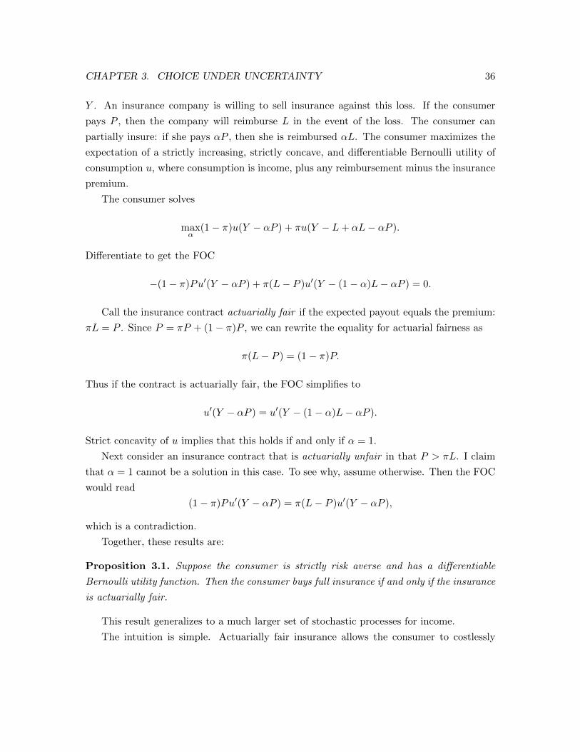
CHAPTER 3. CHOICE UNDER UNCERTAINTY 36
Y . An insurance company is willing to sell insurance against this loss. If the consumer
pays P , then the company will reimburse L in the event of the loss. The consumer can
partially insure: if she pays αP , then she is reimbursed αL. The consumer maximizes the
expectation of a strictly increasing, strictly concave, and differentiable Bernoulli utility of
consumption u, where consumption is income, plus any reimbursement minus the insurance
premium.
The consumer solves
maxα
(1− π)u(Y − αP ) + πu(Y − L+ αL− αP ).
Differentiate to get the FOC
−(1− π)Pu′(Y − αP ) + π(L− P )u′(Y − (1− α)L− αP ) = 0.
Call the insurance contract actuarially fair if the expected payout equals the premium:
πL = P . Since P = πP + (1− π)P , we can rewrite the equality for actuarial fairness as
π(L− P ) = (1− π)P.
Thus if the contract is actuarially fair, the FOC simplifies to
u′(Y − αP ) = u′(Y − (1− α)L− αP ).
Strict concavity of u implies that this holds if and only if α = 1.
Next consider an insurance contract that is actuarially unfair in that P > πL. I claim
that α = 1 cannot be a solution in this case. To see why, assume otherwise. Then the FOC
would read
(1− π)Pu′(Y − αP ) = π(L− P )u′(Y − αP ),
which is a contradiction.
Together, these results are:
Proposition 3.1. Suppose the consumer is strictly risk averse and has a differentiable
Bernoulli utility function. Then the consumer buys full insurance if and only if the insurance
is actuarially fair.
This result generalizes to a much larger set of stochastic processes for income.
The intuition is simple. Actuarially fair insurance allows the consumer to costlessly

CHAPTER 3. CHOICE UNDER UNCERTAINTY 37
replace the risky income with it’s expected value. Wanting to do so is the very definition of
risk aversion. But, with differentiable utility, an expected utility maximizer is approximately
risk-neutral for small risks. Since rejecting the last bit of coverage is taking a small bet
with positive expected value, the consumer wants to do it.
3.3.2 Comparing Risk Aversion
Now we turn to the question of how to compare the risk tolerance of two different decision
makers. The first step is a couple of additional definitions.
Let p be a lottery. If x is a sure thing such that δx ∼ p, then we call x the certainty
equivalent of p. Denote the certainty equivalent of p by C(p), and call R(p) = Ep− C(p)
the risk premium of p. This “functional” notation needs a result that says things are
well-defined:
Theorem 3.3. Suppose preferences are represented by the expectation of a Bernoulli utility
function that is continuous and strictly increasing. Then every p has exactly one certainty
equivalent.
Proof. If p is degenerate, then strict monotonicity directly implies that the only certainty
equivalent is the prize that has probability one.
If p is non-degenerate, then there must be two prizes in the support of p, say x and x, such
that u(x) >∑
x u(x)p(x) and u(x) <∑
x u(x)p(x). Since u is continuous, the intermediate
value theorem implies that there is an x with x < x < x with u(x) =∑
x u(x)p(x). And
strict monotonicity implies that there is only one such.
There is a useful approximation to the risk premium if the risk is “small”—that is, if
all elements in the support of p are close to Ep. By definition, we have
u(Ep−R(p)) =∑x
u(x)p(x).
The LHS can be approximated:
u(Ep−R(p)) ≈ u(Ep)− u′(Ep)R(p).
For any x in the support of p, write:
u(x) ≈ u(Ep) + u′(Ep)(x− Ep) +1
2u′′(Ep)(x− Ep)2.

CHAPTER 3. CHOICE UNDER UNCERTAINTY 38
Take the expected value to get an approximation of the RHS:
∑x
u(x)p(x) ≈ u(Ep) +1
2u′′(Ep)
∑x
(x− Ep)2p(x) = u(Ep) +1
2u′′(Ep) var(p).
Approximately equating the two approximations gives:
u(Ep)− u′(Ep)R(p) ≈ u(Ep) +1
2u′′(Ep) var(p).
Solve for R(p) to get:
R(p) ≈ −u′′(Ep)u′(Ep)
· var(p)
2.
The value of the function λ(x) = −u′′(x)u′(x) is called the coefficient of absolute risk
aversion at x. So we can state the approximation as: for small risks, the risk premium
is approximately the coefficient of absolute risk aversion times half the variance. This
suggests, correctly, that comparing coefficients of absolute risk aversion lets us compare the
risk aversion of different decision makers.
Now we can start comparing. Subscript C, R, and λ with the utility function that
defines them.
Say that the DM with utility function u is at least as risk averse as the DM with
utility function v if, for all p and all sure things x, if u weakly prefers the lottery p, then so
does v.
Proposition 3.2. Suppose u and v are both strictly increasing and continuously differen-
tiable. Then, the following are equivalent:
1. u is at least as risk averse as v;
2. Cu(p) ≤ Cv(p);
3. there is an increasing and concave function h such that u = h v;
4. λu(x) ≥ λv(x) for all x.
Proof. First we show that (1) ⇔ (2). Each direction will proceed by proving the contra-
positive. We have u is not at least as risk averse as v if and only if there are p and x such
that:Eu(p) ≥ u(x) but Ev(p) < v(x)
⇔ u(Cu(p)) ≥ u(x) but v(Cv(p)) < v(x)
⇔ Cu(p) ≥ x but Cv(p) < x.

CHAPTER 3. CHOICE UNDER UNCERTAINTY 39
But the last line holds for some p and x if and only if Cu(p) > Cv(p) for some p.
Next we show that (2)⇔ (3). Since v is strictly increasing, it has an inverse v−1. So let
h = u v−1. Now we have
Cv(p) ≥ Cu(p) for all p
⇔ u(Cv(p)) ≥ u(Cu(p)) for all p monotonicity of u
⇔ h v(Cv(p)) ≥ u(Cu(p)) for all p u = h v⇔ h(Ev(p)) ≥ Eu(p) for all p definition of C
⇔ h(Ev(p)) ≥ Eh(v(p)) for all p u = h v⇔ h is concave Jensen’s inequality.
Finally, we show (3)⇔ (4). Differentiate the identity u(x) = h(v(x)) to get
u′(x) = h′(v(x))v′(x).
Take logs of both sides and differentiate again to get
u′′(x)
u′(x)=h′′(x)v′(x)
h′(v(x))+v′′(x)
v′(x),
or
−u′′(x)
u′(x)= −v
′′(x)
v′(x)− h′′(x)v′(x)
h′(v(x)).
Thus λu(x) ≥ λv(x) for all x if and only if h is concave.
We can see all of these ideas in action in a more general version of the investment problem
we started with. Recall that DM has wealth W > 0, and will do all of her consumption
in one year. She can divide her wealth between two different securities. We continue to
assume that one security is risk-free and the other is risky, but we are less specific about
the returns. The risk-free security has gross return r > 1, while the risky security pays
gross return θ with simple probability measure π. DM maximizes the expected value of a
Bernoulli utility function u defined over her final wealth Y . Assume u is twice differentiable
with u′(x) > 0 and u′′(x) ≤ 0 for all x.
Our first step is to calculate the expected utility of an arbitrary investment plan. If DM
puts α in the risky security and the return on that security is θ, then final wealth is
Y = θα+ r(W − α) = α(θ − r) + rW.

CHAPTER 3. CHOICE UNDER UNCERTAINTY 40
This wealth is realized with probability π(θ). Thus the expected utility is∑θ∈suppπ
u(α(θ − r) + rW )π(θ).
Let’s assume that DM can borrow money to invest in the risky security, but cannot
short-sell the risky security. In that case, she can choose any α ≥ 0. So her problem is:
maxα
∑θ∈suppπ
u(α(θ − r) + rW )π(θ).
Concavity of u implies concavity of the entire objective function. This means that α∗ is
a solution to the optimization problem if and only if it solves the first-order condition:∑θ∈suppπ
(θ − r)u′(α∗(θ − r) + rW )π(θ) ≤ 0, (3.1)
with equality if α∗ > 0.
There is nothing in our assumptions so far that ensure a solution actually exists. Suppose
θ > r for all θ ∈ supp(π). Then, since u′(x) > 0 for all x, every term in the sum on the LHS
of inequality 3.1 is positive, which means the inequality cannot be satisfied. Intuitively,
the risky asset pays more than the risk-free asset no matter what. Thus DM would like to
borrow arbitrarily large sums to invest in the risky security.
Next suppose DM is risk neutral, so u is linear. That means u′(x) is constant at, say,
k. The FOC then becomes
k∑
θ∈suppπ
(θ − r)π(θ) ≤ 0,
or
k (Eθ − r) ≤ 0.
If Eθ < r, then this implies α∗ = 0 is the unique optimum. But if Eθ = r, then any α is an
optimum. And if Eθ > r, there is again no solution.
From now on, assume that u is strictly concave, and that min supp(π) < r < max supp(π).
This is not enough to guarantee a solution, so further assume there at least one solution.
With these assumptions, we can prove that the solution is unique: differentiate the LHS of
inequality 3.1 with respect to α to get∑θ∈supp(π)
(θ − r)2u′′(α(θ − r) + rW )π(θ) < 0.

CHAPTER 3. CHOICE UNDER UNCERTAINTY 41
What can we say about this solution? First consider the case Eθ ≤ r. I claim that
α∗ = 0 is the solution. Write θ = min supp(π). Then
u′(α(θ − r) + rW ) > u′(α(θ − r) + rW
for all θ > θ. Thus∑θ∈suppπ
(θ − r)u′(α∗(θ − r) + rW )π(θ) <∑
θ∈suppπ
(θ − r)u′(α∗(θ − r) + rW )π(θ)
= u′(α∗(θ − r) + rW )∑
θ∈suppπ
(θ − r)π(θ)
= u′(α∗(θ − r) + rW ) (Eθ − r)
≤ 0.
Now consider the case Eθ > R. I claim that the solution must have α∗ > 0. We know
that there is a solution α∗ ≥ 0. If we rule out α∗ = 0, then the claim must be true.
Substitute α∗ = 0 into the FOC to get
u′(rW ) (Eθ − r) ≤ 0,
which is impossible.
The intuition here is just like in the insurance example—an expected utility maximizer
with a differentiable Bernoulli utility function is approximately risk neutral for small risks.
Now we can do some comparative statics. Imagine that two different DM’s face this
problem, one with utility u and one with utility v. And suppose that u is strictly more risk
averse as v. Finally, assume Eθ > r, so both DMs invest a positive amount in the risky
security.
Let α∗u be the optimal risky investment for utility u and let α∗v be the optimal investment
for utility v. The first-order conditions are∑θ∈suppπ
(θ − r)u′(α∗u(θ − r) + rW )π(θ) = 0 (3.2)
and ∑θ∈suppπ
(θ − r)v′(α∗v(θ − r) + rW )π(θ) = 0. (3.3)

CHAPTER 3. CHOICE UNDER UNCERTAINTY 42
Proposition 3.2 implies that the first of these can be written∑θ∈supp(π)
(θ − r)h′(v(α∗u(θ − r) + rW ))v′(α∗u(θ − r) + rW )π(θ) = 0
for some increasing and strictly concave function h.
I claim that DM with utility v invests more in the risky security as does DM with utility
u—that is, α∗v ≥ α∗u. Intuitively, this is because concavity of h means the LHS of the FOC
for u puts more weight on the negative terms in the sum.
First split the FOC for v into a part with θ > r and a part with θ < r:∑θ<r
(θ − r)v′(α∗v(θ − r) + rW )π(θ) +∑θ>r
(θ − r)v′(α∗v(θ − r) + rW ) = 0.
Next consider a similar splitting in the case of u = h v:∑θ<r
(θ−r)h′(v(α(θ−r)+rW ))v′(α(θ−r)+rW )π(θ)+∑θ>r
(θ−r)h′(v(α(θ−r)+rW ))v′(α(θ−r)+rW )π(θ).
We can bound this expression from above term-by-term. Let θ = maxθ | θ < r. Then∑θ<r
(θ − r)h′(v(α(θ − r) + rW ))v′(α(θ − r) + rW )π(θ)
≤∑θ<r
(θ − r)h′(v(α(θ − r) + rW ))v′(α(θ − r) + rW )π(θ)
= h′(v(α(θ − r) + rW ))∑θ<r
(θ − r)v′(α(θ − r) + rW )π(θ),
where the inequality is because h concave implies h′ is decreasing and each (θ−r) is negative.
(It is not a strict inequality because there might be only one θ < r.)
Similarly, let θ = minθ | θ > r. Then∑θ>r
(θ − r)h′(v(α(θ − r) + rW ))v′(α(θ − r) + rW )π(θ)
≤∑θ<r
(θ − r)h′(v(α(θ − r) + rW ))v′(α(θ − r) + rW )π(θ)
= h′(v(α(θ − r) + rW ))∑θ<r
(θ − r)v′(α(θ − r) + rW )π(θ).

CHAPTER 3. CHOICE UNDER UNCERTAINTY 43
Together, these bounds give us:∑θ<r
(θ − r)h′(v(α(θ − r) + rW ))v′(α(θ − r) + rW )π(θ)
+∑θ>r
(θ − r)h′(v(α(θ − r) + rW ))v′(α(θ − r) + rW )π(θ)
< h′(v(α(θ − r) + rW ))∑θ<r
(θ − r)v′(α(θ − r) + rW )π(θ)
+h′(v(α(θ − r) + rW ))∑θ<r
(θ − r)v′(α(θ − r) + rW )π(θ).
By equation 3.3, we have∣∣∣∣∣∑θ<r
(θ − r)v′(α∗v(θ − r) + rW )π(θ)
∣∣∣∣∣ =∑θ<r
(θ − r)v′(α∗v(θ − r) + rW )π(θ).
By strict concavity of h and
α∗v(θ − r) + rW < α∗v(θ − r) + rW,
we have ∣∣∣∣∣h′(v(α(θ − r) + rW ))∑θ<r
(θ − r)v′(α(θ − r) + rW )π(θ)
∣∣∣∣∣> h′(v(α(θ − r) + rW ))
∑θ<r
(θ − r)v′(α(θ − r) + rW )π(θ).
Since the negative part has greater absolute value, the sum is negative. And since the
derivative of the expected utility for the DM with utility function u is less than that sum,
we have ∑θ∈supp(π)
(θ − r)h′(v(α∗v(θ − r) + rW ))v′(α∗v(θ − r) + rW )π(θ) < 0.
Since the LHS is strictly decreasing in α, this establishes that α∗v > α∗u.
The way we typically relate this result to something that could be observed in data is
to make assumptions about how risk aversion varies with wealth. A plausible assumption
is that risk aversion decreases with wealth: λ(x) is decreasing in x. With this assumption,
the previous result implies that if two DMs have the same Bernoulli utility, the one with
greater initial wealth invests more in the risky security.

CHAPTER 3. CHOICE UNDER UNCERTAINTY 44
And a last observation is that we now understand why the solution to the motivating
example was independent of wealth: risk aversion is constant in wealth, with value λ if and
only if Bernoulli utility has the form − 1λe−λx. (You will provide the details in the problem
set.)
3.3.3 Stochastic Dominance
So far, our comparative statics results have concerned variation in risk preferences, for a
fixed set of lotteries. But it is often useful instead to directly compare lotteries. A standard
approach does this through unanimity theorems—giving conditions on two lotteries such
that all decision makers with Bernoulli utilities in some class agree that the first lottery is
preferred to the second.
To keep things simple, we focus on continuous random variables in this section, and
assume that every random variable considered has a density, and has support contained in
[0, x]. We will also assume that all Bernoulli utility functions are continuous and is twice
differentiable except possibly at finitely many points. This will let us use one of the most
useful facts from calculus: integration by parts. Suppose U and V are differentiable except
possibly at finitely many points, with derivatives U ′ = u and V ′ = v. Then∫ b
aU(x)v(x) dx = U(b)V (b)− U(a)V (a)−
∫ b
aV (x)u(x) dx.
This will be our main tool for this section.
Say that lottery F first-order stochastically dominates lottery G if every DM with
increasing Bernoulli utility function prefers F to G. That is, for all increasing functions u,
we have ∫u(x)f(x) dx ≥
∫u(x)g(x) dx.
The following theorem makes this definition easier to apply.
Theorem 3.4. F first-order stochastically dominates G if and only if F (x) ≤ G(x) for all
x.
Proof. Integrating by parts with V (x) = −[1− F (x)], the expected utility of lottery F is∫ x
0u(x)f(x) dx = u(0) +
∫ x
0u′(x)[1− F (x)] dx.

CHAPTER 3. CHOICE UNDER UNCERTAINTY 45
Similarly, ∫ x
0u(x)g(x) dx = u(0) +
∫ x
0u′(x)[1−G(x)] dx.
Thus∫ x
0u(x)f(x) dx−
∫ x
0u(x)g(x) dx =
∫ x
0u′(x)[1− F (x)] dx−
∫ x
0u′(x)[1−G(x)] dx
=
∫ x
0u′(x)[G(x)− F (x)] dx.
Suppose F (x) ≤ G(x) for all x. Then∫ x
0u(x)f(x) dx−
∫ x
0u(x)g(x) dx =
∫ x
0u′(x)[G(x)− F (x)] dx ≥ 0,
where the inequality follows from the supposition F (x) ≤ G(x) and u′(x) ≥ 0.
Suppose there is an x0 such that F (x0) > G(x0). Since F and G have densities, they
are continuous, and there is an interval (x0− ε, x0 + ε) such that x0− ε < x < x0 + ε implies
F (x) > G(x).
Consider the (weakly) increasing function
u(x) =
1 if x ≥ x0 + εx−(x0−ε)
2ε if x0 − ε < x < x0 + ε
0 if x ≤ x0 − ε.
This function is differentiable except at x0 − ε and x0 + ε, with derivative
u′(x) =
0 if x > x0 + ε12ε if x0 − ε < x < x0 + ε
0 if x < x0 − ε.
For this u, we have∫ x
0u(x)f(x) dx−
∫ x
0u(x)g(x) dx =
1
2ε
∫ x0+ε
x0−ε[G(x)− F (x)] dx < 0,
where the inequality follows from F (x) > G(x) on the interval.
First-order stochastic dominance can be thought of as a “stochastically larger” relation-
ship. It is also interesting to think about ranking random variables in terms of “less risky”.
To do so, we will restrict attention to comparisons of distributions with the same mean.

CHAPTER 3. CHOICE UNDER UNCERTAINTY 46
Say that random variable Y is a mean-preserving spread of random variable X if
there is a random variable Z such that:
1. Y has the same distribution as X + Z, and
2. E(Z | X) = 0 for all X.
That is, Y is equal to X plus noise.
Theorem 3.5. Suppose X is a random variable with distribution F and Y is a random
variable with distribution G, and that E(X) = E(Y ). Then the following statements are
equivalent:
1.∫ x
0 u(x)f(x) dx ≥∫ x
0 u(x)g(x) dx for all concave u;
2.∫ x
0 F (x) dx ≤∫ x
0 G(x) dx for all x ∈ [0, x]; and
3. Y is a mean-preserving spread of X.
I’m going to skip the proof, with the following remarks:
1. The equivalence of points 1 and 2 in the theorem has a proof very similar to Theorem
3.4, with the following changes:
(a) Integrate by parts twice:∫ x
0u(x)f(x) dx = u(x)− u′(x)
∫ x
0F (s) ds+
∫ x
0u′′(x)
∫ x
0F (s) ds dx,
and similarly for∫ x
0 u(x)g(x) dx.
(b) Integrate by parts in the integral for the expected value of X:∫ x
0xf(x) dx = x−
∫ x
0F (s) ds,
and similarly for∫ x
0 xg(x) dx.
(c) Use the equal means condition and u′′(x) ≤ 0 for all x to compare the expected
utilities.
(d) The clever choice of u in the 2⇒ 1 direction has the form x 7→ min(x, x0) for an
appropriately chooses x0.
2. The proof of 3⇒ 1 is a generalization of the argument in Exercise 3.4.

CHAPTER 3. CHOICE UNDER UNCERTAINTY 47
3. Proofs that either 1 or 2 imply 3 are significantly more involved.
4. Terminology here is a bit confusing. Some references call the condition in point 2 of the
Theorem second-order stochastic dominance only when means are equal, while others
talk about second-order stochastic dominance without the equal means condition.
We’ll conclude with two examples of how useful the idea of mean-preserving spreads can
be.
Example 3.1. Consider an investor who must divide her wealth w between
two assets. These assets have returns R1 and R2, which are independent and
identically distributed random variables. The fully diversified portfolio puts half
the wealth into each asset; it has return R = 12R1 + 1
2R2.
Consider some other portfolio, with fraction α in asset 1 and fraction 1− αin asset 2. Its return is
αR1 + (1− α)R2 =1
2R1 +
(α− 1
2
)R1 +
1
2R2 +
(1− α− 1
2
)R2
= R+
(α− 1
2
)R1 +
(1− α− 1
2
)R2.
By Theorem 3.5, we will know that full diversification is optimal for any risk-
averse investor if
E((
α− 1
2
)R1 +
(1− α− 1
2
)R2 | R
)= 0
for all R. By linearity of conditional expectations,
E((
α− 1
2
)R1 +
(1− α− 1
2
)R2 | R
)=
(α− 1
2
)E(R1 | R)+
(1− α− 1
2
)E(R2 | R).
Since R1 and R2 are iid, we must learn the same things about them from ob-
serving their sum, so E(R1 | R) = E(R2 | R). But then,
E((
α− 1
2
)R1 +
(1− α− 1
2
)R2 | R
)=
(α− 1
2
)E(R1 | R)+
(1− α− 1
2
)E(R1 | R) = 0.
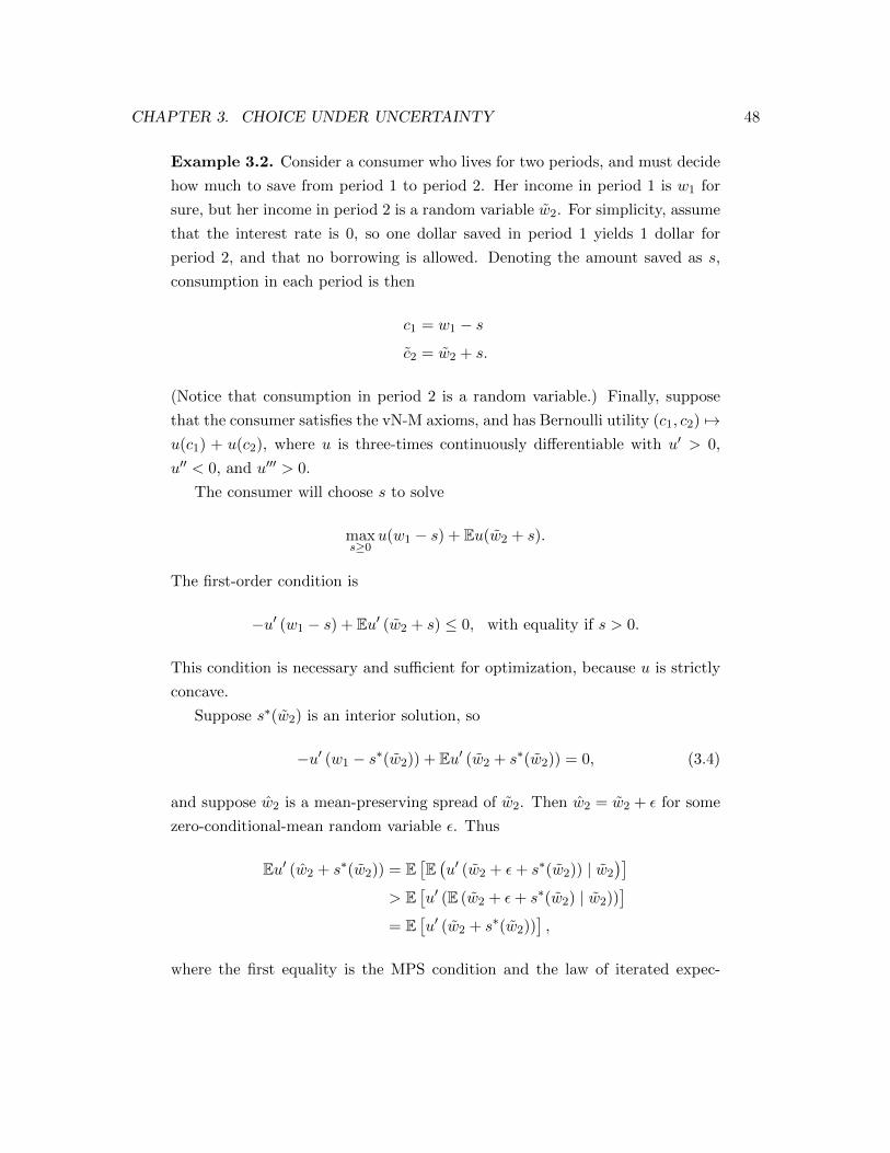
CHAPTER 3. CHOICE UNDER UNCERTAINTY 48
Example 3.2. Consider a consumer who lives for two periods, and must decide
how much to save from period 1 to period 2. Her income in period 1 is w1 for
sure, but her income in period 2 is a random variable w2. For simplicity, assume
that the interest rate is 0, so one dollar saved in period 1 yields 1 dollar for
period 2, and that no borrowing is allowed. Denoting the amount saved as s,
consumption in each period is then
c1 = w1 − s
c2 = w2 + s.
(Notice that consumption in period 2 is a random variable.) Finally, suppose
that the consumer satisfies the vN-M axioms, and has Bernoulli utility (c1, c2) 7→u(c1) + u(c2), where u is three-times continuously differentiable with u′ > 0,
u′′ < 0, and u′′′ > 0.
The consumer will choose s to solve
maxs≥0
u(w1 − s) + Eu(w2 + s).
The first-order condition is
−u′ (w1 − s) + Eu′ (w2 + s) ≤ 0, with equality if s > 0.
This condition is necessary and sufficient for optimization, because u is strictly
concave.
Suppose s∗(w2) is an interior solution, so
−u′ (w1 − s∗(w2)) + Eu′ (w2 + s∗(w2)) = 0, (3.4)
and suppose w2 is a mean-preserving spread of w2. Then w2 = w2 + ε for some
zero-conditional-mean random variable ε. Thus
Eu′ (w2 + s∗(w2)) = E[E(u′ (w2 + ε+ s∗(w2)) | w2
)]> E
[u′ (E (w2 + ε+ s∗(w2) | w2))
]= E
[u′ (w2 + s∗(w2))
],
where the first equality is the MPS condition and the law of iterated expec-

CHAPTER 3. CHOICE UNDER UNCERTAINTY 49
tations, while the last equality is conditional-mean-zero of ε. More interesting
is the inequality. It follows from Jensen’s inequality and the observation that
u′′′ > 0 implies the marginal utility u′ is convex.
Combined with Equation 3.4, we see that s∗(w2) is no longer optimal after
the mean-preserving spread. Since u′ is decreasing, we need to increase s to
compensate. Thus a mean-preserving spread of the second period income leads
to an increase in savings.
Problems
Exercise 3.1. One way to construct preferences over monetary lotteries is to evaluate a
lottery L by the mean EL and the variance var(L). This may or may not be consistent with
the von Neumann-Morgenstern axioms.
1. Show that the preferences represented by U(L) = EL − 14 var(L) do not satisfy the
vN-M axioms. (Hint: Consider the mixtures of the lotteries (1; 1) and (1/2, 1/2; 0, 4)
with the lottery (1/2, 1/2; 0, 2).)
2. Show that the preferences represented by U(L) = EL− (EL)2 − var(L) do satisfy the
axioms.
Exercise 3.2 (Rubinstein). A decision maker has a preference relation % over the space of
lotteries L(X) on a set of prizes X. On Sunday she learns that on Monday she will be told
whether she has to choose between L1 and L2 (probability 1 > α > 0) or between L3 and
L4 (probability 1− α). She will make her choice at that time.
Here are two possible approaches she can take:
Approach 1 Delay her decision until Monday (“why bother with the decision now when I
can make up my mind tomorrow. . . ”).
Approach 2 Make a contingent decision on Sunday regarding what to do on Monday.
That is, she decides what to do if she faces the choice between L1 and L2 and what
to do if she faces the choice between L3 and L4 (“On Monday morning I will be so
busy . . . ”).
1. Formulate Approach 2 as a choice between lotteries.
2. Show that if the preferences of the decision maker satisfy the independence axiom,
then her choice under Approach 2 will always be the same as under Approach 1.

CHAPTER 3. CHOICE UNDER UNCERTAINTY 50
Exercise 3.3. An investor has wealth W and has to decide how much of it to invest in
a risky project that returns θ per dollar invested, where the expected value of θ is greater
than 0. The balance is invested in a riskless asset that returns r per dollar invested, where
Eθ > r > 0. Show that if the investor’s utility function is u(m) = log(m), then the investor
will invest a constant fraction of wealth in the risky project.
Exercise 3.4. Let lottery p = (2/3, 1/3; 10, 20) and lottery p′ = (1/3, 5/9, 1/9; 5, 15, 30).
1. Show that p′ corresponds to a random variable that is the sum of the random variable
corresponding to p and a conditional-mean-zero random variable.
2. Show that any risk-averse expected utility maximizer prefers p to p′. (Show this
directly; do not appeal to Theorem 3.5.)
Exercise 3.5 (MIT). Consider a town not very far from Chicago that is filled with expected
utility maximizing citizens, all of whom have Bernoulli utility function u(w). Assume that
this utility function is differentiable as many times as you like, and further assume it is
strictly increasing and concave.
Every individual has some initial wealth as well as a car which must be parked at metered
parking spaces each day. The cost of the meter is given by m. If the meter is not paid, it
indicates “violation.” The town hires police who patrol the area, and with probability p
the violation is spotted and a fine f is levied. If the police do not spot the violation, the
individual pays nothing.
Consider the problem faced by an individual who maximizes their utility for the day
by choosing whether or not to feed the meter (for non-Americans, “feed” is slang for “put
money into”). Let ∆ denote the returns to the agent from feeding the meter, that is, the
difference between the agent’s expected utility from feeding the meter and their expected
utility from parking illegally.
1. Suppose that the town council considers funding more police, which increases p, versus
raising the fine f . Compute the elasticity of ∆ with respect to p, and compare it to
the elasticity of ∆ with respect to f . To which policy change are the citizens more
responsive?
2. For the remainder of this problem suppose that citizens of this town differ according
to their initial wealth, w0, on the range [w,w]. Suppose also that the parameters of
the problem are such that ∆ is decreasing in initial wealth, and that we observe some
citizens feeding the meters and others parking illegally.

CHAPTER 3. CHOICE UNDER UNCERTAINTY 51
Write a simple expression which determines which group of people feeds meters and
which group parks illegally. Show that the assumption that the both groups are
nonempty requires assuming that the price of the meter, m, is larger than the expected
value of the fine, pf , from parking illegally.
3. Qualitatively, how does the set of people who feed the meters change with f , m, and
p? Prove your answer and interpret your results.
Exercise 3.6. Consider an expected utility maximizer with quadratic Bernoulli utility for
wealth:
u(w) = a+ bw + cw2.
1. What restrictions (if any) must be placed on the parameters a, b, and c for this
decision maker to be risk averse?
2. Over what domain of wealth can this Bernoulli utility represent the preferences of a
decision maker who prefers more to less?
3. Show that if this function satisfies the restrictions from parts (a) and (b), then the
function cannot represent the preferences of a decision maker with decreasing absolute
risk aversion.
Exercise 3.7. Prove that a Bernoulli utility function u has constant absolute risk aversion
λ if and only if it has the form
u(x) = −aλe−λx + b
for constants a > 0 and b.
Exercise 3.8. Consider the insurance problem from lecture, and assume that insurance is
actuarially unfair. Also suppose the buyer has decreasing absolute risk aversion. Show that
her demand for insurance is decreasing in her initial wealth.
Exercise 3.9.
1. Show that, if F first-order stochastically dominates G, then the mean of x under F
is at least as large of the mean of x under G. That is, that∫xf(x) dx ≥
∫xg(x) dx.
2. Give an example where∫xf(x) dx >
∫xg(x) dx but F does not first-order stochasti-
cally dominate G.

Chapter 4
Consumer Theory: A First Look
We are now going to turn to a cornerstone of traditional microeconomics: the problem of a
consumer facing linear prices.
4.1 The Setting
4.1.1 Consumer Preferences
The consumer can conceivably consume any bundle of goods in the set X ⊂ Rn. The subset
is not defined by budget considerations; in the language of abstract decision theory, it is the
set A. It instead reflects considerations like “consumption of food must be nonnegative”.
Indeed, we will often use the special case X = Rn+. But that assumption is sometimes too
restrictive. For example, we can capture restrictions based on location with the following
trick: let good 1 be ice cream in Chicago, and good 2 be ice cream in New York (and assume
there are no other goods). Then we can define
X = (x, 0) | x ≥ 0 ∪ (0, x) | x ≥ 0
to capture the idea that the consumer cannot simultaneously consume ice cream in two
different cities.
By the way, this trick of defining multiple copies of physically similar commodities is
useful in other contexts. We can distinguish ice cream today from ice cream tomorrow, and
ice cream if it is hot outside from ice cream if it is cold outside. These tricks mean that,
even though we are developing the theory as if the world is static with no uncertainty, the
results are more broadly applicable.
52

CHAPTER 4. CONSUMER THEORY: A FIRST LOOK 53
As always, we will assume that the consumer has preferences % on X that are complete,
transitive, and continuous. But the context suggests some additional assumptions.
First, it is often reasonable to assume that the consumer prefers more than less. One
version of this is: preferences are monotonic if x ≥ y implies x % y. We can strengthen
this to rule out indifference: preferences are strictly monotonic if x > y implies x y.
These assumptions will often be reasonable, but are sometimes too strong. Is there
really no limit on how much ice cream you want to eat? And do you want any number of
nickel-alloy-coated electrodes? I doubt it. Nonetheless, I also don’t think many consumers
are going to be happy stopping short of spending their entire income. (Recall that savings
can be handled with dated commodities.) The weakest assumption that captures this is as
follows. Preferences are locally non-satiated if, for any x ∈ X and any ε > 0, there is a
y ∈ X with ‖x− y‖ < ε and y x.
Strict monotonicity⇒monotonicity⇒local non-satiation. Translation of these concepts
to utility representations are immediate.
Another class of assumptions about preferences concern preference for variety, or mixing.
In intermediate micro, this captured by the assumption that indifference curves are bowed
in the direction of the origin. We can make this precise as follows. Preferences are convex
if, for all y ∈ X, the set x ∈ X | x % y is convex. (The set that appears in the definition
is called the upper contour set of y.
Clearly, preferences are convex if and only if every utility representation U has the
property that, for each y, the set x | U(x) ≥ U(y) is convex. In that case, we say that
the function is quasiconcave. An alternative characterization of quasiconvity is this: for
any x and x′ and any λ ∈ [0, 1],
U(x) ≥ U(x′) implies U(λx+ (1− λ)x′) ≥ U(x′).
Preferences are strictly convex if x0 % y and x1 % y (with x0 6= x1) imply λx0 + (1−λ)x1 y for 0 < λ < 1. In the two variable case, this means the indifference curves have
no “flat” segments. In utility terms, this corresponds to strict quasi concavity: for any
x and x′ and any λ ∈ (0, 1),
U(x) ≥ U(x′) implies U(λx+ (1− λ)x′) > U(x′).
Do not confuse concavity and quasiconcavity. Concave functions must be quasiconcave,
but the converse is not true. To see this, observe that any increasing function on the
interval [0, 1] is quasiconcave, even the ones that are strictly convex. What is true is that if

CHAPTER 4. CONSUMER THEORY: A FIRST LOOK 54
a monotone transformation f U is concave, then U is quasiconcave.
4.1.2 The Consumer’s Problem
The classic consumer problem is to choose a consumption bundle to maximize utility given
fixed, linear prices:
maxx∈X
U(x) (4.1)
st px ≤ I (4.2)
Write the solution as x∗(p, I). This is the demand correspondence.
We will make strong assumptions to take the most direct route to the classical theory:
1. Preferences are continuous.
2. Preferences are locally non-satiated.
3. Preferences are strictly convex.
These give us some useful properties:
Theorem 4.1. 1. For any λ > 0, we have x∗(p, I) = x∗(λp, λI).
2. If preferences are continuous and all prices are strictly positive, the consumer’s prob-
lem has a solution.
3. If preferences are locally non-satiated, then at any solution the consumer spends all of
her income: px∗(p, I) = I.
4. If X is convex and preferences are strictly convex, there is at most one solution.
5. If X is convex and there is a unique solution for all (p, I), then the demand function
is continuous.
Proof.
1. The feasible sets are identical.
2. If prices are positive, the budget set is compact. If preferences are continuous, we can
choose a continuous utility representation.

CHAPTER 4. CONSUMER THEORY: A FIRST LOOK 55
3. Suppose x is a bundle that satisfies the budget with strict inequality: px < I. Then
there is an ε > 0 such that yp < I for all y with ‖x − y‖ < ε. But then local non-
satiation implies that there is a y that satisfies both y x and yp < I, so x does not
maximize utility.
4. If x and y 6= x both solve the consumer’s problem, then we must have x ∼ y. But
strict convexity then says 12x+ 1
2y x, contradicting optimality of x.
5. This is immediate from a mathematical result called Berge’s Theorem of the Maxi-
mum. You can read about it in Riley.
The first result says that only relative prices matter.
Since we assume continuity, local non-satiation, and strict convexity, we get a continuous
demand function.
We’d like to be able to answer comparative statics questions about demand. For exam-
ple:
• How does demand vary with income, for fixed prices? (Income effect, Engel curve)
• How does demand vary with price, for fixed income? (Price effect)
4.2 Solving the Consumer’s Problem
To apply these mathematical tools the consumer’s problem, add the assumptions:
4. U is continuously differentiable.
5. For all x ∈ Rk+, we have DU(x) > 0.
Assumptions 1 through 5 are enough for us to appeal to the Kuhn-Tucker Theorem.
Proposition 4.1. Assume 1 through 5. Then x∗ solves the consumer’s problem for prices
p and income I if and only if there is a λ > 0 such that
∂U
∂xj(x∗) ≤ λpj (4.3)
x∗j
(∂U
∂xj(x∗)− λpj
)= 0 (4.4)
px∗ = I (4.5)

CHAPTER 4. CONSUMER THEORY: A FIRST LOOK 56
Proof. A rewriting of the Kuhn-Tucker sufficiency conditions gives the conclusion with
λ ≥ 0.
Since we have DU(x) > 0, we know that ∂U∂xj
(x∗) > 0 for at least one j. If λ = 0, we
would have∂U
∂xj(x∗) > 0 = λpj ,
a contradiction. Thus λ > 0.
We also freely assume the following whenever we want to ignore corner solutions:
Let (xn) be a sequence with limit x, where xj = 0. Then
limx→0
∂U
∂xj(x) =∞.
If this holds, then the FOC for xj cannot be satisfied with xj = 0.
Let’s look at a couple of examples.
Example 4.1. Utility is Cobb-Douglas if
U(x1, . . . , xn) =∏i
xαii
for coefficients αi > 0. The analysis will be simplest if we apply a log transfor-
mation, working with
u(x1, . . . , xn) =∑i
αi log xi.
Once we do this, we might as well divide by a constant to get∑
i αi = 1. This
gives a strictly concave objective, and the marginal utility of xi is αixi
, which
diverges to infinity as xi → 0. Thus we know that any solution will be interior,
and that the FOCs are sufficient. The FOCs simplify to:
αix∗i
= λpi for all i
px∗ = I.

CHAPTER 4. CONSUMER THEORY: A FIRST LOOK 57
Substitute αiλ = pix
∗i into the budget constraint to get∑
i
αiλ
= I,
or
λ =1
I.
Substitute back into the FOC for xi to get demand:
x∗i (p, I) =αiI
pi.
The key implication of Cobb-Douglas demand is that the expenditure share on
good i, namelypix∗i
I , is constant at αi.
Example 4.2. Utility is quasi-linear in the first good if it has the form
U(x1, . . . , xn) = x1 + v(x2, . . . , xn)
for some function v. Let’s consider the case of n = 2 and v strictly increas-
ing and strictly concave. Also assume that v satisfies the Inada conditions:
limx→0 v′(x) =∞ and limx→∞ v
′(x) = 0. The FOCs are
1 ≤ λp1
v′(x2) ≤ λp2
px = I,
with complementary slackness.
The first Inada condition ensures that x∗2 > 0. We need to consider two cases
for x∗1. First, x∗1 might be positive. In this case, the FOCs become
1 = λp1
v′(x2) = λp2
px = I.

CHAPTER 4. CONSUMER THEORY: A FIRST LOOK 58
Eliminate λ to get
v′(x2) =p2
p1.
Since v is strictly concave, this has a unique solution
x2
(p2
p1
)= (v′)−1
(p2
p1
).
If x2(p2/p1) is consumed of good 2, then I − p2x2(p2/p1) is left over for good 1.
If this is non-negative, then demand is
x∗1(p, I) =I − p2x2(p2/p1)
p1
x∗2(p, I) = x2(p2/p1).
However, if I − p2x2(p2/p1) < 0, the previous solution will violate the lower
bound on x1. In that case we must look for a corner solution. The FOCs become:
1 ≤ λp1
v′(x2) = λp2
p2x2 = I.
Substitute the budget into the FOC for x2 to get
v′(I
p2
)= λp2.
Eliminate λ to get
v′(I
p2
)≥ p2
p1.
Since x2 >Ip2
and v is strictly concave, this is in fact a solution. Demand is
x∗1(p, I) = 0
x∗2(p, I) =I
p2.

CHAPTER 4. CONSUMER THEORY: A FIRST LOOK 59
Focus on demand for good 2:
x∗2(p, I) =
I/p2 if x2 >Ip2
x2
(p2p1
)if x2 ≤ I
p2
• Demand is (weakly) decreasing in p2.
• If both goods are demanded in positive amounts, demand for good 2 is
independent of income.
• Demand fails to be differentiable at x2 = Ip2
, even though utility is as
differentiable as we could want.
In addition to solving specific examples, we can also use the Kuhn-Tucker conditions to
recover the intermediate micro characterization of the consumer’s optimum. Suppose two
goods, j and k, are both consumed in positive amounts. Then the FOCs
∂U(x∗)
∂xj= λpj and
∂U(x∗)
∂xk= λpk
can be combined to give∂U(x∗)∂xj
pj=
∂U(x∗)∂xk
pk.
We can get a better understanding of these conditions by thinking about what the
derivatives really mean. Consider some consumption bundle x 0 that satisfies the budget
constraint with equality: px = I. Reducing consumption of good j by ε > 0 will free up pjε
dollars, which will buypjpkε units of good k. This changes consumption from x to x + εd,
where d is a vector with −1 in the jth place,pjpk
in the kth place, and 0 everywhere else.
Taylor’s theorem says
U(x+ εd)− U(x) ≈ DU(x) · (εd) = ε
(−∂U(x∗)
∂xj+pjpk
∂U(x∗)
∂xk
).
If the bracketed term is positive, then, for small enough ε, the change raises utility. If the
bracketed term is negative, then, for small enough ε, a change to x − εd raises utility. At
an optimum, neither of these can be true, so the bracketed term must be zero.
Think about this as follows: the gradient DU(x) tells us the “improving directions” for
U starting at x. Formally, say that vector d is an improving direction at x if there is
an ε such that ε > ε > 0 implies x + ε · d x. The proceeding Taylor argument can be

CHAPTER 4. CONSUMER THEORY: A FIRST LOOK 60
modified to show that, if preferences have a differentiable utility representation, the set of
improving directions is the set d | DU(x) · d > 0.And that observation tells us what the assumption of differentiable utility really means.
The assumption that preferences % can be represented by a differentiable utility function U
just means that, for each x, there is a vector v(x) such that the set of improving directions
d is d | v · d > 0. That is, the set of improving directions is a half-space defined by the
hyperplane normal to v.
An example of preferences that are not differentiable are given by Leontieff utility:
U(x1, . . . , xn) = minxk. Any improving direction must have all components positive. But
that is inconsistent with the set of improving directions being a half-space.
So far, we’ve seen that DU(x) tells us the directions in which small changes increase
utility. As is so often the case, adding convexity allows a “local to global” translation: If
preferences are convex as well as differentiable, then the upper contour set of x lies on one
side of the hyperplane normal to DU(x).
We will show this in a more general setting, so we can use it later to study production
and welfare economics.
Theorem 4.2. If g is differentiable and Y = y | g(y) ≥ g(y0) is convex, then
y ∈ Y =⇒ Dg(y0) · (y − y0) ≥ 0.
Proof. Choose any y ∈ Y . By convexity of Y ,
yλ ≡ λy + (1− λ)y0 ∈ Y
for all λ ∈ [0, 1]. Since Y is an upper contour set, this is equivalent to
g(yλ)− g(y0) ≥ 0.
Define h(λ) = g(yλ) = g(y0 + λ(y − y0)). Then
h(λ)− h(0)
λ=g(y0 + λ(y − y0))− g(y0)
λ.
For any λ ∈ (0, 1), the RHS is ≥ 0, since yλ ∈ Y . Thus the limit
limλ→0
h(λ)− h(0)
λ≥ 0.

CHAPTER 4. CONSUMER THEORY: A FIRST LOOK 61
But that limit is just the derivative of h, so h′(0) ≥ 0.
By the chain rule,
dh
dλ(λ) = Dg(y0 + λ(y − y0)) · (y − y0).
Set λ = 0 then gives
Dg(y0)(y − y0) ≥ 0,
as desired.
4.3 Empirical Implications of CP
Now we turn to a discussion of what the classical theory of the consumer implies for data.
Consider the following situation. You observe the bundle that some particular consumer
would select for each of a finite set of price-income combinations. (Perhaps this is hypo-
thetical data from a survey; perhaps it is actual choice data from a sequence of decision
problems that are sufficiently delinked to treat as separate problems.) What observations
would refute the hypothesis that the consumer made her choices according to the model of
this chapter?
Start with the case of just two observations. In particular, suppose there are two goods,
1 and 2, and the price-income pairs are (pa, Ia) = ((1, 2), 10) and (pb, Ib) = ((2, 1), 10).
And suppose the consumer chooses bundle xa = (2, 4) when facing (pa, Ia) and chooses
xb = (4, 2) when facing (pb, Ib). In each case, the consumer spends her entire budget. But
pa · xb = 8 < 10, and similarly for pb · xa.These two inequalities are not necessarily a problem for the hypothesis that the consumer
is maximizing a rational preference relation. After all, she might be globally indifferent, in
which case any choice at any price-income pair is ok. But that response rather trivializes
the question. And if we add the assumption that the consumer’s preferences are supposed
to be locally non-satiated, the two inequalities are a problem for our hypothesis. To see
this, we will use the following:
Lemma 4.1. Suppose that a consumer maximizes a complete, transitive, and locally non-
satiated preference by choosing x when prices are p and income is I. If x′ is some bundle
such that px′ ≤ I, then x % x′. And if x′ is some bundle such that px′ < I, then x x′.
Proof. If px′ ≤ I but x′ x, then x would not be preference maximizing at prices p and
income I. Now consider some x′ such that px′ < I. There is an ε > 0 such that, for any z

CHAPTER 4. CONSUMER THEORY: A FIRST LOOK 62
with ‖z − x′‖ < ε, we have pz < I. But local non-satiation implies that, for at least one of
those z, we have z x′. If x′ % x, transitivity would imply z x, contradicting optimality
of x.
Going back to the example, since paxb < Ia, we must have xa xb. But pbxa < Ib
implies xb xa. These two strict preferences can’t both hold, so the observations are not
consistent with the standard model.
In that example, the violation of the hypothesis was particularly stark. But more subtle
violations can be detected using transitivity. Consider the following choices.1
• At prices (10, 10, 10) and income 300, the consumer chooses (10, 10, 10).
• At prices (10, 1, 2) and income 130, the consumer chooses (9, 25, 7.5).
• At prices (1, 1, 10) and income 11, the consumer chooses (15, 5, 9).
Applying Lemma 4.1 to the first two bullet points tells us that (9, 25, 7.5) % (10, 10, 10).
Applying Lemma 4.1 to the last two bullet points tells us that (15, 5, 9) (9, 25, 7.5). And
applying Lemma 4.1 to the first and last bullet points tells us that (10, 10, 10) (15, 5, 9).
But those three preferences together are inconsistent with transitivity.
You might fear now that we can keep on creating ever more new problems. But don’t
worry—we have in fact seen examples of everything that can go wrong. The main technical
result of this section is designed to make this reassurance precise.
Definition 4.1. Suppose there is a finite set of demand observation of the form: x1 is
chosen at (p1, I1), x2 is chosen at (p2, I2), and so on.
1. If pixj ≤ Ii, then xi is directly revealed preferred to xj, written xi %D xj. If
pixj < Ii, then xi is directly revealed strictly preferred to xj, written xi D xj.
2. xi is revealed preferred to xj, written xi %R xj, if either xi %D xj or there is a
sequence (xk)Kk=1 such that
xi %D x1 %D · · · %D xK %D xj .
If, furthermore, at least one of the directly revealed preferences is strict, then xi is
revealed strictly preferred to xj, written xi N xj.
1This example is taken from Kreps (2012), p. 67.

CHAPTER 4. CONSUMER THEORY: A FIRST LOOK 63
3. If the set of observations satisfy the generalized axiom of revealed preference, or
GARP if there are no cycles in the revealed strictly preferred to relation, that is, if
there is no i such that xi R xi.
Theorem 4.3 (Afriat). If a finite set of demand data violate GARP, then the data are
inconsistent with the maximization of a complete, transitive, and locally non-satiated pref-
erence relation. Conversely, if a finite set of demand data satisfy GARP, then the data
are consistent with consistent with maximization of a preference relation that is complete,
transitive, strictly increasing, continuous, and convex.
The proof of the first claim is an easy combination of Lemma 4.1 and the argument
about transitivity in the second example. The proof of the second claim is much harder;
see Kreps (2012) §4.2 if you are interested, though be warned the proof will not teach you
any techniques useful elsewhere in microeconomics.
This definition and theorem are a lot to digest all at once, so let me give you some
pointers.
1. In the definition, I never say that i 6= j. Thus, if pixi < Ii, we can conclude that
xi D xi, which implies xi R xi, which is a violation of GARP.
2. Comparing the two statements in the Theorem shows that strengthening local non-
satiation to strict monotonicity, adding continuity, or adding convexity to the assump-
tions of completeness, transitivity, and local non-satiation does nothing to the model’s
ability to accommodate the data. Said differently, those extra assumptions have no
testable implications for market demand data.
3. The last point does not mean that the additional properties have no testable assump-
tions at all. For example, we could ask the consumer to rank the three bundles x, x′,
and 12x + 1
2x′. If she tells us that x 1
2x + 12x′ and x′ 1
2x + 12x′, then know she
does not have convex preferences. The point, rather, is that market demand data can
never reveal this failure of convexity.
4.3.1 Empirical Applications
One way that GARP and Afriat’s theorem are useful is in applications with real data. Two
prominent examples come from experimental studies of altruism and from the economics of
the family.2
2This subsection borrows heavily from lecture slides by Parag Pathak.

CHAPTER 4. CONSUMER THEORY: A FIRST LOOK 64
Experimental economists study altruism in the context of the dictator game: one sub-
ject chooses how to divide a sum of money between herself and a second subject. The second
subject makes no decisions—whatever the first subject decides is implemented. If subjects
were rational and selfish, maximizing their own wealth, the first subject would simply keep
all of the money. That is not what happens—many subjects give away significant amounts.
Selfishness is often a useful assumption, but it is certainly not entailed by rationality.
So it is interesting to ask if behavior in the dictator game is consistent with rational and
altruistic preferences. A famous paper by Andreoni and Miller (Econometrica, 2002) tackles
this.
They have subjects make a sequence of decisions of the form:
Here are M tokens. Divide them between yourself and an anonymous other
subject. You will get x cents for each token you keep, and the other subject will
get y cents for each token you give them.
Think of the parameters (M,x, y) as determining income and the relative price of money
for the self and money for the other—the subject might be thought of as solving
maxcs,co
u(cs, co)
st1
xcs +
1
yco ≤M.
If this interpretation is a good approximation to what people do in the experiment, their
choices should satisfy GARP. Andreoni and Miller find that 156 of their 176 subjects are
fully consistent with GARP, and most of the others would have no violations if only a few
tokens were reallocated. A couple of subjects had many violations.
Another example concerns the economics of the family. Although the theory we have
developed is usually motivated as a theory of the individual, it is often applied at the
household level. Whether or not this is a good idea depends on how decision-making inside
of families works. One model of the family (introduced by Gary Becker) has a single member
(typically the father) making the decisions, usually (hopefully?) with altruistic motivation.
If that is how families work, the standard model of the consumer will work well. But it
will be more problematic if there is non-trivial bargaining within the family. In that case,
the distribution of bargaining power, and thus decision power, can be affected by which
member of the family brings certain resources.
Duflo (World Bank Economic Review, 2003) found a nice natural experiment to shed
light on this question, based on an unexpected grant of a large pension to black South

CHAPTER 4. CONSUMER THEORY: A FIRST LOOK 65
African retirees. Whether the money was received by the grandmother or grandfather had
a big impact on how the funds were spent. More money is spent on female children when
grandmothers get the money than when grandfathers do. And the effect is more pronounced
for the mother’s mother than for the father’s mother.
A Beckerian household would satisfy GARP, and thus could only display the effect
found by Duflo if the decision maker were indifferent between spending on daughters or
other things. That is possible, I guess. But interpreting the regularity of the association as
a strict preference for spending more on daughters from female-acquired income than from
male-acquired income implies that GARP is violated, and the household is not Beckerian.
4.3.2 Downward-Sloping Demand?
You will sometimes hear people talk about the “Law of Demand”—the claim that demand
curves slope down. This is a pretty good approximation empirically, but it is not in fact an
implication of the model we are considering in this chapter.
From intermediate micro, you know that goods for which the law of demand fails are
called Giffen goods. And you have probably seen pictures of indifference curves that generate
Giffen behavior. We can use Afriat’s Theorem to rigorize such pictures.
Fix prices p and income I, and suppose the consumer chooses x. Let new prices be p′
where pj = p′j for all goods j 6= i, and p′i > pi. Let x′ be any bundle that satisfies the
budget constraint with equality: p′x′ = I. In particular, we allow for x′i > xi
Given the construction, we must have p′x > px = I. Since the original bundle is
not affordable at the new prices, there cannot be any violation of GARP in just these
two observations. And Afriat’s Theorem then implies that there is a well-behaved utility
function that is maximized at x when prices are p and at x′ when prices are p′.
Another thing that you recall from intermediate micro is that stronger results are pos-
sible if we consider price changes accompanied by “compensating” income changes. We can
use Afriat’s Theorem to study the Slutsky compensation, the one that keeps income fixed
at the whatever level makes the original bundle just affordable at the new prices.
Theorem 4.4. Suppose a consumer chooses x when facing prices p and income I, and
chooses xs when facing prices are p′, where pj = p′j for j 6= i and p′i > pi, and income p′x.
If the choices maximize a complete, transitive, and locally non-satiated preference relation,
then xsi ≤ xi.
Proof. By local non-satiation, xs must satisfy the budget constraint with equality: p′xs =
p′x. Note that this immediately implies xs %R x

CHAPTER 4. CONSUMER THEORY: A FIRST LOOK 66
Writing out the budget constraint, we have∑j 6=i
p′jxsj + p′ix
si =
∑j 6=i
p′jxj + p′ixi.
Substitute p′j = pj for j 6= i to get∑j 6=i
pjxsj + p′ix
si =
∑j 6=i
pjxj + p′ixi.
Suppose, to get a contradiction, that xsi > xi. Since we know that p′i > pi, we can
conclude that (p′i − pi)xsi > (p′i − pi)xi. Subtract the larger term from the LHS of the
displayed equation to get∑j 6=i
pjxsj + p′ix
si − (p′i − pi)xsi =
∑j 6=i
pjxsj + pix
si .
Subtract the smaller term from the RHS of the display to get∑j 6=i
pjxj + p′ixi − (p′i − pi)xi =∑j 6=i
pjxj + pixi.
Since we subtracted the larger term from the LHS of the equality, we have∑j 6=i
pjxsj + pix
si <
∑j 6=i
pjxj + pixi,
or pxs < px. And that implies that x R xs, so we have a violation of GARP.
The name “Slutsky compensation” might have already told you what is coming next.
We can use income effects to formally link the (observable) uncompensated demand change
with the (signable) compensated demand change. This is the Slutsky equation.
As before, write x for demand at prices p and income I, and xs for demand at prices p′
and income p′x. In addition, write x′ for demand at prices p′ and income I. Since
x′i − xi = (xsi − xi)− (xsi − x′i),
we can divide by ∆pi = p′i − pi > 0 to get
x′i − xi∆pi
=xsi − xi
∆pi− xsi − x′i
∆pi. (4.6)

CHAPTER 4. CONSUMER THEORY: A FIRST LOOK 67
The Slutsky compensation adjusts the consumer’s income by ∆I = ∆pi ·xi. Substitute this
into equation 4.6 to getx′i − xi
∆pi=xsi − xi
∆pi− xi
xsi − x′i∆I
.
The first term on the right-hand side is the compensated effect that is signed by Theorem
4.4. The second term depends on the difference xsi − x′i. These demands arise from the
same prices, but with different incomes. Thus the ratioxsi−x′i
∆I has a natural interpretation
as an income effect. This income effect is weighted by the initial demand for good i.
4.3.3 Aggregating Demand
There is another gap between what the theory predicts and the usual statement of the “Law
of Demand”. Namely, the law is usually thought of as holding for market demand, while
the theory we have been developing is at the individual level.
If aggregating demand across consumers preserved the restrictions that individual de-
mand has to satisfy, then this would be a reasonable lapse. But it does not.
Afriat’s Theorem makes this easy to see. Suppose that, in a two-consumer, two-good
economy, each consumer always has income 1000. If prices are (10, 10), consumer 1 chooses
(25, 75) and consumer 2 chooses (25, 75). If prices are (15, 5), consumer 1 chooses (40, 80)
and consumer 2 chooses (64, 8). You should verify that neither consumer violates GARP,
and so each is consistent with our theory.
Now calculate market demands. If prices are (10, 10), market demand is (100, 100). If
prices are (15, 5), market demand is (104, 88). These demands violate GARP—(100, 100)
equals total income at both price vectors, and (10, 10) · (104, 88) = 1920 < 2000.
Problems
Exercise 4.1. Suppose u is a utility representation of preferences % and f is a strictly
increasing function. Show that if f u is concave, then preferences are convex.
Exercise 4.2. Suppose u is a utility representation of preferences %. Show that, if there
is a strictly increasing function f such that
f u(x) =
m∑j=1
vj(x),
where each vj is concave, then preferences are convex.

CHAPTER 4. CONSUMER THEORY: A FIRST LOOK 68
Exercise 4.3 (Rubinstein). Consider the preference relations on the interval [0, 1] that are
continuous. What can you say about those preferences which are also strictly convex?
Exercise 4.4. Consider the following three utility functions (in each case, α1, α2 > 0):
1. U(x1, x2) = α1√x1 + α2
√x2
2. U(x1, x2) = α1x1 + α2x2
3. U(x1, x2) = min(α1x1, α2x2)
For each, answer the following:
(a) Are the preferences monotone? Strictly monotone?
(b) Are the preferences convex? Strictly convex?
(c) For each, calculate the demands for strictly positive prices (p1, p2) 0 and income
I. (For utility functions (1) and (2), use the Kuhn-Tucker conditions. For part (3),
explain why the Kuhn-Tucker Theorem does not apply, and then find the demands
anyway.)
Exercise 4.5. Suppose the consumer’s utility function is defined as follows:
U(x1, x2, x3, x4) = min (x1 · x2, x3 · x4) .
Find the demand function.
Exercise 4.6. An infinitely lived consumer owns 1 unit of cake that she consumes over
her lifetime. The cake is perfectly storable and she will receive no more than she has now.
Consumption of cake in period t is denoted xt, and her lifetime utility function is given by
U(x0, x1, . . .) =
∞∑t=0
δt log xt,
where 0 < δ < 1.
Calculate her optimal level of cake consumption in each period.
(Note: The statement of the Kuhn-Tucker theorem in class was for finite dimensional
problems. But it also applies to this problem, even though there are infinitely many choice
variables.)

CHAPTER 4. CONSUMER THEORY: A FIRST LOOK 69
Exercise 4.7. A consumer consumes 2 commodities, wheat and candy. His utility from
consuming w units of wheat and c units of candy is
3 logw + 2 log c.
He faces 4 constraints:
• Consumption of each good must be nonnegative.
• The consumer has $10 to spend, and the price of each good is $1.
• The consumer is on a diet, and cannot consume more than 1550 calories. A unit of
wheat has 150 calories, and a unit of candy has 200 calories.
Follow the following steps to solve this consumer’s problem:
1. Derive the Kuhn-Tucker optimality conditions for this consumer’s problem.
2. Are the conditions derived above sufficient for this problem? Why or why not?
3. Explain why the conditions from part (1) imply consumption of both commodities
must be positive.
4. Explain why the conditions from part (1) imply that at least one of the budget and
calorie constraint must bind.
5. Look for a solution the the conditions from part (1) in which only the budget constraint
binds.
6. Look for a solution the the conditions from part (1) in which only the calorie constraint
binds.
7. Look for a solution the the conditions from part (1) in which both constraints bind.
Exercise 4.8 (Rubinstein). Consider a consumer with a preference relation in a world
with two goods, X (an aggregated consumption good) and M (“membership in a club”, for
example), which can be consumed or not. In other words, the consumption of X can be
any nonnegative real number, while the consumption of M must be either 0 or 1.
Assume that the consumers preferences are strictly monotonic and continuous and satisfy
the following property:

CHAPTER 4. CONSUMER THEORY: A FIRST LOOK 70
Prices Income Demandp1 p2 p3 Y x1 x2 x3
1 1 1 20 10 5 53 1 1 20 3 5 61 2 2 25 13 3 31 1 2 20 15 3 1
Table 4.1: Data for Exercise 4.9.
Property E: For every x, there is a y such that (y, 0) (x, 1) (i.e., there is
always some amount of the aggregated consumption good that can compensate
for the loss of membership).
1. Show that the consumer’s preferences can be represented by a utility function of the
form:
u(x,m) =
x if m = 0
x+ g(x) if m = 1.
2. Explain why continuity and strong monotonicity (without property E) are not suffi-
cient for the result in part 1.
3. Calculate the consumer’s demand function.
Exercise 4.9 (Kreps). In a three good world, a consumer has demands given by Table
4.3.3. Are these choices consistent with the maximization of a complete, transitive, and
locally non-satiated preference relation?
Exercise 4.10. True, false, or uncertain. Explain your answer.
1. “You cannot derive a demand function for lexicographic preferences.”
2. “The behavior of a consumer with lexicographic preferences is empirically indistin-
guishable from that of a consumer who only gets utility from a single good.”

Chapter 5
Production
The next important class of decision-maker we will study are producers. The intermediate
micro treatment of producers goes like this: a firm produces output Y using inputs labor,
L, and capital, K, according to the production function F . The firm buys inputs at prices
w for labor and r for capital, and sells output at price p. The firms wants to maximize
profit, so it solves
maxL,K
pF (L,K)− wL− rK.
This problem is easiest to solve if F is strictly concave and differentiable. Then an
interior solution is characterized by the first order conditions:
p∂F
∂L(L,K) = w and p
∂F
∂K(L,K) = r.
These two equations implicitly define two functions, L∗(w, r) and K∗(w, r), called the factor
demands.
We will pay attention to several questions as we generalize this model.
1. How can we handle multiple outputs?
2. Can we treat a collection of profit-maximizing producers as a single, aggregate pro-
ducer?
3. What is the connection between profit maximization and the efficient allocation of
resources?
To give a sense of the importance of these questions, we will take a brief look at the
model economists typically use to think about the skill distribution and income inequality.
71

CHAPTER 5. PRODUCTION 72
This model is based on an aggregate technology and is clearly related to normative concerns,
so the second and third questions take on an obvious importance.
Our approach to these questions will be to treat production as a special case of the
rational choice model from Chapter 1. The set A will be all conceivable production plans,
while the feasible plans will be represented by a set Y called a technology.
Our treatment of technologies will be general, but we will restrict attention to a very
special case of preferences—maximization of profit at fixed prices. Sometimes this is of-
fered as a good descriptive model of firms in a competitive market. It is often a useful
first approximation there, but we should note how weak the common justification for the
assumption really is. That justification is that profit maximization is what owners of the
firm want. But:
1. How do we know owners agree? They typically do not when markets are incomplete
or the firm has market power.
2. How relevant are owners’ wishes? Modern economies are characterized by a separation
of ownership and control. This creates principal-agent problems that complicate any
simple relationship between what owners want and what actually happens.
Nonetheless, the profit-maximizing producer is central to microeconomic theory. Partly
this is because, in many applications, the conceptual problems mentioned above don’t seem
to matter much in practice. But this is also because the profit-maximizing producer provides
the simplest example of the link between prices and efficiency.
5.1 Technology
We will work in Rn, with the interpretation that each dimension i measures the quantity
of some good i. Think of production as changing the set of stuff in the world—starting
from some status quo ω ∈ Rn, the act of production changes things so that the collection
of goods is ω′ ∈ Rn. We call the increment y = ω′ − ω a production plan.
Typically, production will use some goods to produce others. That is, some components
of y will be positive (net inputs) and others will be positive (net outputs). Reflecting this,
production plans are sometimes called netput vectors.
A technology is a set Y of production plans. Some useful assumptions:
Nonempty Y is a nonempty set.
Closed Y is a closed set.

CHAPTER 5. PRODUCTION 73
No free lunch Y ∩ RK++ = ∅. In words, producing any output requires some input.
Irreversability Suppose y ∈ Y and y 6= 0. Then −y 6∈ Y .
These first four assumptions are basically technical, and we won’t make a big deal out of
them. The next two are substantive.
Possibility of inaction 0 ∈ Y . Thinking back to intermediate micro, this says there are
no sunk costs. It is perfectly consistent with fixed cost.
Free disposal If y ∈ Y and y′ ≤ y, then y′ ∈ Y . Throwing things away is costless.
More interesting for us will be the idea of returns to scale.
Nonincreasing returns to scale If y ∈ Y and α ∈ [0, 1], then αy ∈ Y . That is, any
feasible netput vector can be scaled down.
Nondecreasing returns to scale If y ∈ Y and α ≥ 1, then αy ∈ Y . That is, any feasible
netput vector can be scaled up.
Constant returns to scale If y ∈ Y and α ≥ 0, then αy ∈ Y . That is, any feasible
netput vector can be scaled up or down.
A particularly useful assumption is:
Convexity Y is a convex set.
Think of this as combing two ideas:
1. Nonincreasing returns. (If inaction is possible and technology is convex, then it has
nonincreasing returns.)
2. “Balanced” input combinations are at least as productive as “unbalanced”. Similarly,
“Balanced” output combinations are no more expensive than “unbalanced”.
Sometimes it makes sense to separate the goods into inputs and outputs. This is par-
ticularly useful when there is just one output. In that case, we can describe a technology
with a production function, f . If Y is a technology for which good 1 is the output, let
f(z) = supxx | (x,−z) ∈ Y .
(Note that sup ∅ = −∞.)
CHAPTER 5. PRODUCTION 74
Alternatively, if we are given a production function f , we can define Y by
Y = (x,−z) | x ≤ f(z).
(Note the slippage due to free disposal being built into second definition.)
In the single-output case, we can restate the returns to scale assumptions in terms of
the production function.
• Nonincreasing returns: f(αx) ≥ αf(x) for all α ∈ [0, 1] and x.
• Nondecreasing returns: f(αx) ≥ αf(x) for all α ≥ 1 and x.
• Constant returns: f(αx) = αf(x) for all α ≥ 0 and x.
• Convexity: f is concave.
Our definition of a technology is more flexible than one based on production functions,
since we can have multiple outputs and don’t need a priori distinction of input/output.
5.2 Profit Maximization
Let p be a vector in Rn+ interpreted a prices. Then the profit of plan y is py. By our sign
convention on production plans, this really does correspond to our ordinary definition of
profit: outputs are positive and so make a positive contribution, while inputs are negative
and so make a negative contribution. To see this a bit more formally, write
y+ = (max(y1, 0), . . . ,max(yn, 0)) and y− = − (min(y1, 0), . . . ,min(yn, 0)) .
Then y = y+ − y− and
py = py+︸︷︷︸revenue
− py−︸︷︷︸costs
.
The profit maximization problem is
maxy
py
st y ∈ Y
Call the set of solutions to this problem y∗(p). (As we will see, it is very important that we
allow this set to have many elements.)

CHAPTER 5. PRODUCTION 75
Example 5.1. Consider a technology that transforms a single input, x, into a
single output, q, according to the production function x 7→√x. Write z = −x.
Then the technology can be represented by the production possibility set
Y = (q, z) | q ≤√
(−z) and z ≤ 0.
If prices are p = (1, 12), then the profit-maximization problem is
maxq,z
1q +1
2z
st q ≤√
(−z).
Maximization implies not throwing away output, so this is equivalent to
maxz
√(−z) +
1
2z.
The FOC is
− 1
2√
(−z)+
1
2= 0.
Since the objective function in the simplified problem is strictly concave, the
FOC tells us that the unique solution is z = −1.
An important contrast between consumer theory and producer theory concerns exis-
tence of solutions. In consumer theory, existence is is guaranteed under weak continuity
assumptions as long as prices are strictly positive. This is not true for profit maximization.
Theorem 5.1. Suppose Y has nondecreasing returns to scale and some production plan y ∈Y has strictly positive profit at prices p. Then there is no solution to the profit maximization
problem at prices p.
Proof. Suppose y is a feasible production plan with py > 0. Let α be a number greater
than 1. By nondecreasing returns to scale, αy ∈ Y . And
p(αy) = α(py) > py,
which implies y is not profit maximizing. Since y was arbitrary, there is no profit-maximizing
plan.

CHAPTER 5. PRODUCTION 76
Corollary 5.1. Suppose Y has constant returns to scale. Then either maximized profit is
0 or there is no solution to the profit maximization problem.
Proof. Constant returns implies the possibility of inaction, so profits are at least 0. And
the theorem implies that either profits are nonpositive or the profit maximization problem
has no solution.
Example 5.2. Fix a β ∈ R++ and consider the technology
Y = (q, z) | q ≤ −βz and z ≤ 0 ⊂ R2.
If the price vector is (p1, p2) and the production plan is (βx,−x) for some x > 0,
then profit is
p1(βx)− p2x = (p1β − p2)x.
If (p1β − p2) > 0, then there is no solution, and if (p1β − p2) < 0, then the only
solution is x = 0. Moreover, if p2p1
= β, then profits are 0 for any x, and the
solution to the profit maximization problem is indeterminate.
Example 5.3. Now consider a technology that can transform good 2 into good
1 on a one-for-one basis, but only if a fixed amount of one unit of good 1 is used
to start the technology. Formally,
Y = (q, z) | q ≤ −z + 1 and z ≤ 1 ∪ (0, z) | 0 ≤ z < 1 ⊂ R2.
If the price vector is (p1, p2) and the production plan is (x − 1,−x) for some
x ≥ 1, then profit is
p1(x− 1))− p2x = (p1 − p2)x− p1.
If (p1 − p2) > 0, then this is increasing without bound and there is no solution.
If (p1 − p2) ≤ 0, then this is negative for all x. But the feasible plan (0, 0) gives
profit 0. Thus there are no prices at which profits are maximized with positive
output.

CHAPTER 5. PRODUCTION 77
5.3 Aggregate Production
We saw in Chapter 4 that the theory of the consumer does not aggregate nicely, in the
sense that aggregate demand does not satisfy the restrictions implied by maximizing utility
subject to a market budget constraint. Aggregation is much more satisfying for producers.
In this section, we will see a formalization of this claim, and then use it as an excuse to
look at the standard model economists use to think about skill-based income inequality.
The setting will be an economy with several producers, labeled i = 1, . . . , n. Each of
these producers has a technology Y i, which is nonempty and closed. Define the aggregate
production set by
Y agg =
n∑i=1
Y i ≡ y | ∃(y1, . . . , yn) with, ∀i, yi ∈ Y i and y =n∑i=1
yi.
In words, Y agg is the set of all netput vectors that can be constructed as sums of netput
vectors feasible for the individual producers, with exactly one feasible netput vector per
producer.
Now we can define the set of aggregate-profit-maximizing netput vectors:
yagg∗ = arg maxy∈Y agg
py.
Theorem 5.2. yagg∗(p) =∑n
i=1 yi∗(p).
Proof. We want to show that two sets are equal, so we must show 1.) yagg∗(p) ⊂∑ni=1 y
i∗(p) and 2.)∑n
i=1 yi∗(p) ⊂ yagg∗(p).
1. Suppose y ∈ yagg∗(p), but, seeking a contradiction, that y 6∈∑n
i=1 yi∗(p). Let
(y1, . . . , yn) be an arbitrary profile with yi ∈ Y i for all i and y =∑n
i=1 yi. Since
y 6∈∑n
i=1 yi∗(p), there is some j and yj ∈ Y j such that pyj > pyj . Denote by
(y1, . . . , yn) the profile with yi = yi for i 6= j and yj = yj , and let y =∑n
i=1 yi. Sum
over i to get
py = pyj +∑i 6=j
pyi > pyj +∑i 6=j
pyi = py,
so y does not maximize profits over Y agg, a contradiction.
2. Suppose y ∈∑n
i=1 yi∗(p). Let y be an arbitrary element of Y agg, and let (y1, . . . , yn)
be an arbitrary profile with y =∑n
i=1 yi and, for all i, yi ∈ Y i.

CHAPTER 5. PRODUCTION 78
Since y ∈∑n
i=1 yi∗(p), there is a decomposition of y into a profile (y1, . . . , yn) with
y =∑n
i=1 yi and, for all i, yi ∈ yi∗. But that means, for all i, we have pyi ≥ pyi. Sum
over i to get
py =n∑i=1
pyi ≥n∑i=1
pyi = py.
Since y was arbitrary, y ∈ yagg∗(p).
We will see in the next section that convexity of production sets is a very important
property. It is preserved under aggregation.
Theorem 5.3. Suppose each Y j is convex. Then Y agg is convex.
Proof. Exercise 5.3.
Theorem 5.2 is an important part of the background for many applied arguments. A
recently prominent example is the standard framework economists use to think about skill-
based wage inequality.
Imagine an economy with n workers. H of these worker are high skilled, and L are low
skilled. Each of these workers has one unit of labor to supply.
The economy produces output, y, from low-skilled labor, l, and high-skilled labor, h,
according to an aggregate production function:
y = [(All)ρ + (Ahh)ρ]1/ρ.
We assume that Ah > Al and ρ ≤ 1. The second of these assumptions implies that the
production function is concave.
Let’s look for a set of prices (py, pl, ph) = (1, wl, wh) such that, at those prices, profit
maximization is consistent with full employment: l = L and h = H. Since the production
function is concave, the necessary and sufficient conditions are the following first-order
conditions:
wl = Aρl [Aρl +Aρh(H/L)ρ](1−ρ)/ρ
wh = Aρh[Aρh +Aρl (H/L)−ρ](1−ρ)/ρ = Aρh[Aρh(H/L)ρ +Aρl ](1−ρ)/ρ ·
((H/L)−ρ
)(1−ρ)/ρ

CHAPTER 5. PRODUCTION 79
From this we can define the skill premium, denoted ω, by
ω =whwl
=
(AhAl
)ρ(HL
)−(1−ρ)
.
Empirical economists prefer to write this in terms of an object called the elasticity of
substitution. You can read about what this means in general in other sources. Here, I’ll
just note two facts. First, for our production function, the elasticity of substitution, σ, is a
simple function of ρ:
σ =1
1− ρ.
Second, the empirical consensus is that, for the U.S. economy, σ is between 1.5 and 2.
In elasticity of substitution terms, the skill premium is:
ω =
(AhAl
)(σ−1)/σ (HL
)−1/σ
This is particularly easy to understand if we take logs:
logω =
(σ − 1
σ
)log
(AhAl
)− 1
σlog
(H
L
)Given the empirical consensus about σ, we see two implications. First, skill-biased tech-
nological change (i.e., technological changes that increase Ah more than Al) will increase the
skill premium. Second, increases in the fraction of workers who are high-skilled will decrease
the skill premium. Claudia Goldin and Larry Katz have written a lovely book, The Race
Between Education and Technology, interpreting the history of technological innovation,
education policy, and wage inequality over U.S. history in these terms.
From our point of view in this course, the essential point is that all of this only makes
sense because of Theorem 5.2. The history recounted by Goldin and Katz is not one in which
there was a single, centrally controlled technology. Instead, there were many different firms,
each independently trying to maximize profits. Theorem 5.2 tells us that the analysis is
nonetheless legitimate.
5.4 Prices from Efficiency
Given technology Y , the production plan y0 is production efficient if there is no y ∈ Ysuch that y > y0. In other words, if y0 is production efficient, then there is no other feasible

CHAPTER 5. PRODUCTION 80
plan that yields at least as much of everything and strictly more of something.
Prices p support the production plan y0 if
1. py0 ≥ py for all y ∈ Y , and
2. py0 > py for all y ∈ intY . (Note that this implies only boundary points can be
supported.)
From the definition, we see that if there is any supporting price vector for y0, then there
are many—if p supports y0 then so does λp for any scalar λ > 0.
There is a close connection between production efficiency and support by prices.
Proposition 5.1. If y0 is supported by strictly positive prices p, then y0 is production
efficient.
Proof. If y > y0, then py > py0, since p is strictly positive.
Since p supports y0, we must have y 6∈ Y .
The reverse direction, that any efficient plan can be supported by prices, is not true
without additional conditions.
Theorem 5.4 (Supporting Hyperplane Theorem). Suppose Y is a nonempty, convex subset
of Rn, and that y0 is on the boundary of Y . Then there is a p 6= 0 such that:
1. for all y ∈ Y , we have p · y ≤ p · y0 and
2. for all y ∈ intY , we have p · y < p · y0.
We will derive a special case from the following fundamental fact:
Lemma 5.1. If g is differentiable and Y = y | g(y) ≥ g(y0) is convex, then
y ∈ Y =⇒ Dg(y0) · (y − y0) ≥ 0.
Proof. Choose any y ∈ Y . By convexity of Y ,
yλ ≡ λy + (1− λ)y0 ∈ Y
for all λ ∈ [0, 1]. Since Y is an upper contour set, this is equivalent to
g(yλ)− g(y0) ≥ 0.

CHAPTER 5. PRODUCTION 81
Define h(λ) = g(yλ) = g(y0 + λ(y − y0)). Then
h(λ)− h(0)
λ=g(y0 + λ(y − y0))− g(y0)
λ.
For any λ ∈ (0, 1), the RHS is ≥ 0, since yλ ∈ Y . Thus the limit
limλ→0
h(λ)− h(0)
λ≥ 0.
But that limit is just the derivative of h, so h′(0) ≥ 0.
By the chain rule,
dh
dλ(λ) = Dg(y0 + λ(y − y0)) · (y − y0).
Set λ = 0 then gives
Dg(y0)(y − y0) ≥ 0,
as desired.
Proof of supporting hyperplane (for the differentiable case). Assume, in addition
to the hypotheses of the theorem, that there is a differentiable function g such that
Y = y | g(y) ≥ g(y0),
and Dg(y0) 6= 0. By Lemma 5.1, y ∈ Y implies Dg(y0)(y − y0) ≥ 0. Take p = −Dg(y0) to
get
Dg(y0)(y − y0) ≥ 0 ⇐⇒ p(y0 − y) ≥ 0 ⇐⇒ py0 ≥ py.
To provide a converse to Proposition 5.1, we need to know that the supporting prices
are nonnegative. But the Supporting Hyperplane Theorem does not guarantee that. But
one more assumption will do it.
Proposition 5.2. Let Y be a non-empty, convex technology that satisfies free disposal.
If y0 ∈ Y is production efficient, then there is a non-negative price vector p such that p
supports y0. If, in addition, 0 ∈ Y , then py0 ≥ 0.
Proof. Suppose y0 is production efficient. Then there is no y ∈ Y with y > y0, so y0 is
a boundary point of Y . By the Supporting Hyperplane Theorem, there is a price vector
p 6= 0 such that py0 ≥ py for all y ∈ Y .

CHAPTER 5. PRODUCTION 82
We need to show that p > 0.
Write ei for the vector whose components are 0 except for the ith, which is 1. By free
disposal, y1 = y0 − ei ∈ Y . But py0 ≥ py1 implies
p(y0 − y1) = pei = pi ≥ 0.
If in addition 0 ∈ Y , that p is a supporting price implies
py0 ≥ p · 0 = 0.
Example 5.4. Consider again the technology in Example 5.1:
Y = (q, z) | q ≤√
(−z) and z ≤ 0.
To use our theorems, introduce the function g(q, z) =√
(−z)− q. Then we
can rewrite
Y = (q, z) | g(q, z) ≥ 0 and z ≤ 0.
Differentiate
d
dz
√(−z) = − 1
2√
(−z)
d2
dz2
√(−z) = − 1
4(−z)3/2
< 0.
Since sums of concave functions are concave, this implies g is concave, hence
quasi concave.
A production plan (q, z) is efficient if and only if q =√−z. Thus two efficient
plans are
(q, z) = (1,−1) and (q, z) = (2,−4).

CHAPTER 5. PRODUCTION 83
In the first case, the derivative of g is
Dg(1,−1) =
(−1
−12
),
so the supporting prices are p = −D(1,−1) = (1, 1/2). And our analysis from
before shows that the plan (1,−1) in does in fact maximize profits at these
prices.
Now consider the other efficient plan. The derivative is
Dg(2,−4) =
(−1
−14
),
so the supporting prices are p = −D(2,−4) = (1, 1/4).
To check this, consider the maximization problem
max(q,z)∈Y
1 · q +1
4z.
Maximization implies not throwing away output, so this is equivalent to
maxz
√(−z) +
1
4z.
The FOC is
− 1
2√
(−z)+
1
4= 0,
which holds only at z = −4.
5.5 Decentralization via Prices
We have seen that, if technology is convex, prices can guide a producer to an efficient
production plan. Now we will consider a (very simple) complete economy, and see that
prices work well there also.
There are two agents in the economy, a consumer and a producer.
The consumer has preferences % defined on Rn+, and an endowment ω ∈ Rn+.
• Throughout this section, assume that % are represented by a concave and continuously
differentiable utility function U , with DU(x) 6= 0 for all x.

CHAPTER 5. PRODUCTION 84
• The endowment represents the goods the consumer owns prior to any production. In
many examples, the only non-produced good will be labor. Taking labor to be good
one, we can then write the endowment as ω = (L, 0 . . . , 0), where L > 0 is the amount
of time the consumer can work.
The producer has a technology Y ⊂ Rn that is:
• Nonempty, closed, and satisfies no free lunch, irreversibility, and possibility of inaction.
• Y = y | g(y) ≥ g(0) for some concave function g with g(0) = 0.
If the producer chooses the production plan y, then final resources in the economy will
be ω + y. The consumer must then consume some bundle x with x ≤ ω + y.
A first perspective about what this economy should do comes from a benevolent planner,
who sits outside the system and seeks to maximize the consumer’s utility. This planner will
solve:
maxx,y
U(x)
st ωi + yi − xi ≥ 0 for all i
g(y) ≥ 0
xi ≥ 0 for all i
Since U and g are both concave, the Kuhn-Tucker conditions are necessary and sufficient
for a solution. That is, (x∗, y∗) is a solution if and only if:
∂U
∂xi(x∗)− qi ≤ 0 with equality if x∗i > 0
qi + µ∂g
∂yi(y∗) = 0,
where qi ≥ 0 is the multiplier on the resource constraint for good i and µ ≥ 0 is the
multiplier on the production constraint.
Something very important has happened. Prices, in the form of the multipliers qi, have
just appeared.
First, solve the second FOC to get
1
µq = −Dg(y∗).
That is, 1µq supports production plan y.

CHAPTER 5. PRODUCTION 85
Second, the first FOC has a similar interpretation. Consider an interior solution, so the
FOC becomes:
DU(x∗) = q.
This says that −q defines a supporting hyperplane to the set of bundles that the consumer
prefers to x∗. And that means that any bundle better than x∗ is also more expensive.
There is another way to reach the same allocation. Suppose that the consumer owns both
the initial endowment and the technology. But she does not run the technology herself—
instead, it is run by a manager who always maximizes profit. The only way that the
consumer and manager interact is through price-mediated transactions. (This is artificial
in this simple economy, but the ideas generalize to large numbers of both consumers and
producers.)
If prices are p, the producer will solve
maxy
py
st g(y) ≥ 0.
The FOC for this problem is
p = γDg(y).
Denote maximized profits by π(p) = py.
If prices are p, the consumer will solve
maxx
U(x)
st pω + π(p)− px ≥ 0.
The FOC for this problem is
DU(x) ≤ λp.
Say that p is a Walrasian equilibrium price if markets clear:
x︸︷︷︸demand
= ω + y︸ ︷︷ ︸supply
.
Notice that, at a WE price, the cost of the consumer’s demand px, is exactly equal to her
income p(ω + y) = pω + π(p).
Finally, notice that, if p = 1µq, λ = µ, and γ = 1, there is an exact correspondence

CHAPTER 5. PRODUCTION 86
between the necessary and sufficient conditions for the planners solution and the conditions
for the Walrasian equilibrium.
Both approaches lead to the same allocation. This is not a coincidence. There are an
important pair of theorems, called the First and Second Welfare theorems, that generalize
these results to arbitrary numbers of consumers and producers. We’ll see these generaliza-
tions soon.
5.6 Appendix: Subjective Probability
Although it really has nothing to do with production, this is an opportune spot to clear up
a few loose ends from the discussion of subjective probability from Section 3.2. The link to
this chapter is the supporting hyperplane theorem.
Recall the setup:
1. There is a set of states of nature, Ω.
2. There is a set of consequences, X.
3. An act is a map a : Ω→ X.
We will follow the classical development due to Ramsey and de Finetti, which involves two
simplifications. First, assume that Ω is finite. This assumption is not needed for the kind
of result we are aiming for, but it simplifies the mathematics considerably. The second
assumption is more substantive—assume that X = R. The interpretation is that a(ω) is
the amount of money won or lost if the state is ω. (When this assumption is in force, we
often refer to an act as a bet.)
We assume that the DM has complete, transitive, and continuous preferences % over
the set of all possible bets. These preferences satisfy the following additional axioms:
Additivity For all x, y, z, we have x % y if and only if x+ z % y + z.
Monotonicity If x ≥ y, then x % y.
Non-triviality There exist x and y such that x y.
These assumptions are not entirely satisfactory—the following proposition shows that
they imply expected value maximization. More advanced treatments give expected utility
maximization instead. Basically, this involves combining the idea of the following proof
with the independence axiom and the proof of the von Neumann-Morgenstern Theorem.

CHAPTER 5. PRODUCTION 87
Proposition 5.3. Preferences % over bets are complete, transitive, continuous, additive,
monotone, and satisfy non-triviality if and only if there exists a probability vector p such
that
x % y if and only if px ≥ py.
Proof. Necessity is left as an exercise.
By additivity, x % y if and only if 0 % y − x. Thus we can fully describe preferences
over bets by saying which bets are worse than the zero bet, which is naturally interpreted
as “no bet”. This is the set of unacceptable bets,
B = x | 0 % x.
The key observation is the following:
Lemma 5.2. Suppose % satisfies continuity and additivity. Then the set of unacceptable
bets is convex.
Sketch of the proof. Suppose x, y ∈ B satisfy x % y. Let z = x+y2 , so
z − x = y − z =y − x
2≡ d.
Then additivity gives
x % z ⇔ x+ d % z + d⇔ z % y.
Since x % y, the assumption that z x would imply z y, contradicting z % y. Thus
x % z. A similar argument gives z % y, so we have
x %1
2x+
1
2y % y.
Next consider x % y and λx+ (1−λ)y, where λ is a dyadic rational : λ = k2i
for integers
k, i ≥ 1. An inductive version of the previous paragraph yields
x % λx+ (1− λ)y % y.
Continuity then extends the conclusion to any real λ ∈ [0, 1], and transitivity then
implies 0 % λx+ (1− λ)y.
Now we can use the supporting hyperplane theorem. The set B is nonempty because it
contains 0, and we just saw that it is convex. Now we need a boundary point.

CHAPTER 5. PRODUCTION 88
By non-triviality, there is a bet x such that 0 x. By convexity of A, for any ε > 0,
we can take ‖x‖ < ε. But additivity gives −x 0, so the ball y | ‖y‖ < ε contains points
inside of and outside of B.
Putting all of this together, Theorem 5.4 tells us that there is a q 6= 0 such that x is
unacceptable only if q · x ≤ q · 0 = 0.
Now assume that x is not in B, so x 0, but q · x < 0. By additivity, we would have
0 −x and q · (−x) > 0, a contradiction. Thus we have
• x ∈ B ⇒ q · x ≤ 0; and
• q · x < 0⇒ x ∈ B.
But continuity implies that A is closed, so A includes its boundary q · x = 0, which closes
the gap between the two implications.
Next we argue that each qi ≥ 0. Let ei be the unit vector in direction i. By monotonicity,
0 % −ei. Thus q · (−ei) = −qi ≤ 0.
Since q 6= 0, we can normalize:
qx ≤ 0⇔ px ≡ 1
‖q‖(qx) ≤ 0.
Together, the last two points imply that p is a vector of probabilities.
Now we just unpack the meaning of unacceptable bet:
x % y ⇔ 0 % y − x⇔ p · (y − x) ≤ 0⇔ px ≥ py.
That is, x % y if and only if the expected value of x is greater than the expected value of
y.
Problems
Exercise 5.1. Suppose a technology Y is convex and has the property that, if y0 and y1
are both in Y and α ∈ (0, 1), then αy0 + (1 − α)y1 is not production efficient in Y . Show
that, if prices are strictly positive, there is at most one solution to the profit maximization
problem.
Exercise 5.2 (Binmore). Suppose that a profit-maximizing producer chooses a production
plan from a technology Y that is compact and satisfies the property from the previous

CHAPTER 5. PRODUCTION 89
exercise. Write s(p) for the supply function:
s(p) = argmaxy∈Y py.
Answer the parenthetical questions in the following “proof” that the supply function is
continuous, and point to a flaw in the argument. What can be done to patch up the proof?
Let pk → p as k → ∞. Write yk = s(pk). Then, for any z ∈ Y , we have
pkz ≤ pkyk. (Why?) If yk → y, it follows that, for any z ∈ Y , we have pz ≤ py.
(Why?) Hence y = s(p). (Why?) Thus s(pk) → s(p) as k → ∞, and so s is
continuous.
Exercise 5.3. Prove Theorem 5.3.
Exercise 5.4 (Rubinstein). An event that could have occurred with probability 0.5 either
did or did not occur. A firm must provide a report in the form of “the event occurred” or
“the event did not occur”. The quality of the report (the firms product), denoted by q, is
the probability that the report is correct. Each of k experts (input) prepares an independent
recommendation that is correct with probability 1 > p > 0.5. The firm bases its report on
the k recommendations in order to maximize q.
1. Calculate the production function q = f(k) for (at least) k = 1, 2, 3.
2. We say that a discrete production function is concave if the sequence of marginal
product is nonincreasing. Is the firms production function concave?
Assume that the firm will get a prize of M if its report is actually correct. Assume that the
wage of each worker is w.
3. Explain why it is true that if f is concave, the firm chooses k∗ so that the k∗th worker
is the last one for whom marginal revenue exceeds the cost of a single worker.
4. Is this conclusion true in our case?
Exercise 5.5. Using a carefully labeled figure, give an example of a production technology
Y , a production plan y ∈ Y , and prices p ≥ 0 such that
• y is not efficient in Y , but
• y maximizes profits at prices p.

CHAPTER 5. PRODUCTION 90
Exercise 5.6. Draw the hyperplanes and closed half spaces in R2 determined by each if
the following vectors.
1. p = (1, 2)
2. p = (1,−2)
3. p = (−1,−2)
Exercise 5.7. Suppose commodity 1 can be used to produce commodity 2 according to
the technology
Y = (y1, y2) | y1 ≤ 0 and g(y) = −y1 − y2 − y32 ≥ 0.
1. Show that Y is a convex set.
2. Show that the production plan y = (−10, 2) is on the boundary of this set.
3. Calculate the supporting prices for the production plan y.
4. Verify directly that y maximizes profits at the prices you calculated in the previous
step.
5. Depict the production set and the supporting line in a neat figure.
Exercise 5.8 (Riley). Robinson Crusoe lives alone on an island off the coast of New
Zealand. He has a production set
Y = (−z1, y2)|y2 ≤ 16z1/31 , z1 ≥ 0
and an endowment vector ω = (32, 0).
His preferences are represented by the utility function U(x) = log x1 + log x2 .
1. Solve for his optimal choice of input and hence his optimal production plan and
consumption plan x∗.
2. Depict the production set and the set Y +ω in a neat figure and indicate the optimal
production and consumption plans. Explain what it means for the optimal production
plan to be supported by a price vector p = (p1, p2).
3. Solve for the price vector that supports the optimal production plan.

CHAPTER 5. PRODUCTION 91
4. Depict this supporting price line, Crusoes budget set, and indifference curve though
x∗.
5. Hence explain why the supporting price vector is a WE price vector if Robinson Crusoe
is a price-taker.
Chapter 6
Welfare Economics
We are now going to spend a little time on the standard economist’s approach to normative
evaluation. Along the way, we’ll talk about the very beginnings of the theory of competitive
equilibrium, although you’ll have to wait until next quarter for a detailed study of markets.
As you go through a public policy education, it is easy to become complacent about
the normative commitments of practices like cost-benefit analysis. Much attention must be
paid to technical developments. And practical economists like to minimize the contribution
ethical stances make to their policy recommendations. It is crucial to step back and see that
there are substantive normative claims inextricably mixed with science in economics-based
policy advice.
The general setting has a set of allocations A ⊂ Rn, with typical element a, and a
collection H of individuals, each with a utility function uh : A→ R.
An important example covers the division of a fixed bundle of commodities.
Example 6.1. An exchange economy is a tuple
E = 〈H,K, (%h)h∈H , ω〉,
where
• H is the (finite) set of consumers,
• K is the (finite) set of commodities,
• %h is consumer h’s preference over the commodity space RK+ , and
• ω ∈ RK+ is the social endowment.
92
CHAPTER 6. WELFARE ECONOMICS 93
We assume that each preference is complete, transitive, continuous, monotonic,
and convex, with utility representation uh.
An allocation is an array x = (xh)h∈H . An allocation is feasible if
1. xh ∈ RK+ for all h, and
2.∑
h xh ≤ ω.
Write A for the set of feasible allocations.
It will be convenient to stack the utility function as u : A→ Rn, where a 7→(uh(a)
)h∈H .
Such a vector of utility levels is called a utility imputation. The set of all utility impu-
tations, U = x ∈ Rn | ∃a st x = u(a), is called the utility possibility set.
We have been treating preferences as the consumer’s reasons for her choices. The exercise
we are about to undertake will keep this assumption, and add another: that the consumer’s
preferences accurately reflect her welfare.
This is not always reasonable—think of children. It seems better for adults, but even
there psychologists question the link between choices and welfare (projection bias, weakness
of will, etc.). See the article by Kahneman and Varey in Elster and Roemer (eds.) Interper-
sonal Comparisons of Well-Being. In addition to these failures of choices to reflect welfare
as understood by the agent, we may even be concerned that the agent’s conception of her
welfare is different than her true welfare. Sen gives the example of the “tamed housewife”,
who has no options other than being a housewife and adjusts her aspirations downward.
6.1 Normative Concepts for Welfare Economics
Consider a policy analyst, you for short. You want to give policy advice based on your
own preferences about how this economy should operate. Now, I know very little about
you. I certainly don’t know what you think about the aims of public policy. What I do
know is what assumptions I need to make about you to believe you should subscribe to the
standard approach of welfare economics.
Assumption 1 Your normative stance is fully captured by a complete, transitive prefer-
ence % over A. (In fact, I’ll go ahead and assume that your preferences are sufficiently
well-behaved to be represented by a utility function V : A→ R.)
In addition, I need to assume that your preferences respect the preferences of the indi-
viduals in society. To state the relevant assumption, I will use the following formal notions.

CHAPTER 6. WELFARE ECONOMICS 94
Allocation x Pareto dominates y if x %h y for all h and x k y for some k. Allocation x
is Pareto optimal if there is no feasible y which Pareto dominates x.
We can translate our definitions of Pareto dominance, etc into the space of utilities. Al-
location a Pareto dominates a′ if u(a) > u(a′). The set of utility imputations corresponding
to the set of all Pareto optimal alternatives is called the Pareto frontier.
Now we can continue with the assumptions.
Assumption 2 Your preferences respect Pareto dominance: u(a) > u(a′) implies V (a) >
V (a′).
Assumption 3 Your preferences respect Pareto indifference: u(a) = u(a′) implies
V (a) = V (a′).
Theorem 6.1. Fix utility representations uh for the consumers. Your preferences are
represented by a function V that respects Pareto dominance and Pareto indifference if and
only if
V (a) = W (u(a))
for some function W : Rn → R that is strictly increasing on U .
Proof. First, given a function W that is strictly increasing on U , we can define V by V (a) =
W (u(a)). This obviously satisfies the conditions. Now assume that your preferences satisfy
the three assumptions. The first says that there is a V that represents your preferences.
Take any r ∈ U . By the definition of U , there is an a ∈ A such that u(a) = r. Define W (r)
to be V (a) for the associated a. This is well-defined by Pareto indifference, and is strictly
increasing on U because the preferences respect Pareto dominance. To complete the proof,
arbitrarily extend W to all of Rn.
Functions W of the sort introduced in the proposition are called social welfare func-
tionals. Some standard examples are:
1. W (u1, . . . , un) =∑
i ui, the utilitarian social welfare functional.
2. Let αi be strictly positive weights, and let W (u1, . . . , un) =∑
i αiui. This defines
a weighted utilitarian or Bergsonian social welfare functional.
3. W (u1, . . . , un) = minui | i ∈ N, the maximin social welfare functional. (This is
sometimes called the Rawlsian social welfare functional, although that is not entirely
fair to John Rawls.)

CHAPTER 6. WELFARE ECONOMICS 95
This W is not quite a social welfare functional, since it is not strictly increasing. If
it represents your preferences, then you require a strict version of Pareto dominance
before you conclude V (a) > V (a′).
It’s easy to get confused about the meaning of W . Kreps writes:
Note well that the function W defined on Rn depends crucially on the par-
ticular ui that are chosen to represent the preferences of the individual con-
sumers. We could, for example, replace u1 with a function u′1 given by u′1(a) =(u1(a) + 1000
)3(which is a strictly increasing transformation), and then we
would have to change how W responds to its first argument. [p. 159, notation
adjusted to conform to our notation]
The point is that you do not have preferences directly over utility imputations. Instead,
you have preferences over A, and use W only to give a convenient representation of those
preferences.
We now have all the pieces needed to discuss how social welfare functionals are used
in the characterization of Pareto optimal allocations and in the foundations of cost-benefit
analysis. But before we go into that, I want to highlight how strong the assumptions really
are.
• Assumption 1 says that your preferences are defined directly on the set of allocations.
As a result, you cannot distinguish between two identical allocations that are arrived
at in different ways. A particular allocation might be arrived at as the result of the free
choices of individuals; the same allocation might be reached by the fiat of a dictator.
You are blind to the difference. You are similarly blind to things like equality of
opportunity and desert.
• If these omissions bother you, you could try augmenting the description of a social
state to include details about process in addition to the allocation itself. But the
Pareto assumptions will only allow this fix if the consumers value the process the
same way you do. Amartya Sen gave the following example to make this problem
vivid. There are three social states, x, y, and z, and there are two people, 1 and 2.
Their utilities areu1 u2
x 4 10
y 7 8
z 7 8

CHAPTER 6. WELFARE ECONOMICS 96
In state x, 1 is hungry and 2 has enough to eat; in state y, some food has been
transferred from 2 to 1; and in state z, the food allocation is as in x, but 1, a sadist,
is whipping 2. Pareto indifference says that you are indifferent between y and z. I
conclude that my preferences do not satisfy Pareto indifference.
• The previous point shows that Pareto indifference may be problematic. But it is
just the principle of respect for Pareto dominance extend to ensure continuity of your
evaluation function V . As such, problems with Pareto indifference suggest that Pareto
dominance itself might be problematic as a normative guide. In Sen’s example, would
you feel better about the whipping if person 2 held back just enough that person 1
very, very slightly preferred being whipped to the loss of resources?
• Once you’ve ruled out anything but allocations and preferences as subjects for evalu-
ation, it seems natural to take preference satisfaction as the ultimate goal. And that
is what is happening in Theorem 6.1. Sen’s example illustrates one reason to back
away from preference satisfaction as the goal: some preferences might themselves be
normatively objectionable.
There are other reasons to be wary about preference satisfaction as the ultimate goal.
One is lack of information. Assume that a person prefers that no one use cell phones
because of he believes it creates a large risk of cancer. He is wrong about the science.
Must we treat that preference the same way he treat his preference, based on his
subjective sense of tastiness, for oranges over bananas?
• Another problem with the preference-satisfaction view arises when preferences can
change over time. Someone, let’s call him Scott, might prefer to exercise tomorrow
rather than not exercise. But, when tomorrow rolls around, his preferences change,
and he prefers not exercising over exercising. Which preference is normatively rele-
vant?
• The problem of changing tastes is even more pressing when the polices being consid-
ered will lead to different preferences. Whether or not behavioral economics pans out,
these policy-dependent preferences will continue to be a problem for people interested
in child development, education, and related policy areas.
• An even knottier problem of which preferences should be satisfied arises when dif-
ferent policies lead to different populations. For example, consider two development
assistance policies, just one of which has the effect of reducing fertility. What does it
even mean to talk about the preferences of someone who only exists under one policy?

CHAPTER 6. WELFARE ECONOMICS 97
6.2 Characterizing Efficient Allocations
6.2.1 Bergen-Samuleson Social Welfare Functionals
It’s immediate from our assumptions that any maximizer of a social welfare functional is
Pareto optimal. It turns out that we cannot further refine the set of possible social welfare
optima.
Theorem 6.2. Suppose that A is convex and that each uh is concave. If a∗ is Pareto
optimal, then there exists a set of nonnegative weights αi, at least one positive, such that
a∗ ∈ arg maxa∈A
∑i
αiui(a).
(Note that the theorem requires weakening the definition of a social welfare functional
in the same way that the maximin rule did.)
Proof. The result is an application of the supporting hyperplane theorem. To start, we
need to define the convex set we will work with. Let U be the extension of U to satisfy free
disposal:
U = x ∈ Rn | ∃a st x ≤ u(a).
I claim that U is convex. Given that, suppose u∗ is the utility imputation of a Pareto
optimal allocation. The Supporting Hyperplane Theorem says that there is a vector α 6= 0
such that, for all u ∈ U , ∑h
αh(u∗)h = αu∗ ≥ αu =∑h
αhuh,
with strict inequality for u ∈ int U . Since U has free disposal, u ∈ U and δ ≥ 0 imply that
uδ = u− δ ∈ U . By the implication of the supporting hyperplane,
α(u∗ − u∗δ) = αδ ≥ 0
for all δ ≥ 0. If αh were negative, taking δ = −eh would then give a contradiction.1
All that remains is to prove the claim. Let u and u′ be two utility imputations in U .
This implies that there are allocations a and a′ with u ≤ u(a) and u′ ≤ u(a′). Convexity of
A implies that, for any λ ∈ [0, 1], the convex combination a = λa + (1 − λ)a′ is also in A.
1Notation: ek is the unit vector in direction k.

CHAPTER 6. WELFARE ECONOMICS 98
By concavity of uh, we have
λuh(a) + (1− λ)uh(a′) ≤ uh(λa+ (1− λ)a′) = uh(a)
for each h. Stacking these inequalities gives
λu+ (1− λ)u′ ≤ λu(a) + (1− λ)u(a′) ≤ u(a).
In some sense, this is a disappointing result. It says that assumptions 1–3, for all
that they rule out, are not enough to get beyond Pareto dominance as a collectively shared
normative standard. But there is also a positive side. The result gives us a way to completely
characterize the implications of Pareto optimality. This is, in fact, how it is most often used.
6.2.2 Efficient Allocations of Commodities
Let’s see this in our exchange economy example. Recall that an allocation is feasible if
1. xh ∈ RK+ for all h, and
2.∑
h xh ≤ ω.
These clearly define a convex set. And an allocation is Pareto efficient if it maximizes some
weighted sum of (concave) utility representations. So the Pareto optimal allocations are
the solutions to
max(xh)h∈H
∑h
αhuh(xh) (6.1)
st xhj ≥ 0 for all h and j (6.2)
ω −∑h
xhj ≥ 0 for all j (6.3)
Let qj be the shadow price of the adding up constraint for good j. The Kuhn-Tucker
conditions are
αh∂
∂xjuh(xh)− qj ≤ 0 with equality if xhj > 0, for all h and j (6.4)
ωj −∑h
xhj ≥ 0 and qj ≥ 0 with complementary slackness, for all j (6.5)

CHAPTER 6. WELFARE ECONOMICS 99
Since the utilities are concave, these conditions are necessary and sufficient for an allocation
to solve the optimization problem.
If we assume that Duh 0, then all of the resource constraints must hold with equal-
ity, and their shadow prices must be positive. If we further restrict attention to interior
allocations, we get a simple condition:
αhDuh(x∗h) = q for all h.
Now take some consumers h and two goods, j and k. We have, as part of the above,
αh∂
∂xjuh(xh) = qj (6.6)
αh∂
∂xkuh(xh) = qk. (6.7)
Divide to get∂∂xj
uh(xh)
∂∂xk
uh(xh)=qjqk,
which says that consumer h’s MRS between j and k equals the ratio of shadow prices for
the resource constraints of j and k. And since h, j, and k were arbitrary, this implies that
all consumers have equal MRS’s for all pairs of goods.
So if we find (at an interior allocation) that two consumers do not have the same MRS
for some pair of goods, we know there exists a Pareto improvement.
All of this should remind you very much of consumer theory, suggesting that markets
might work well. We’ll turn to that in a moment. But first, there are some caveats that
should always be kept in mind when applying these ideas to policy analysis.
• The presumption that Pareto inefficient allocations are bad is often over interpreted.
What might be uncontroversial is that a Pareto dominated allocation is bad because
one of the allocations that Pareto dominates it is better. This is very different than
claiming that any Pareto optimal allocation is better than any Pareto inefficient allo-
cation. That claim is very hard to justify.
• One justification often given for the second claim is that, after moving from a Pareto
inefficient allocation to a Pareto optimal one, it is then possible to make transfers
from winners to losers so that we have a genuine Pareto improvement. One problem
with this is that it is not true. (It is true in an exchange economy. But the claim can
fail in more complicated problems.)

CHAPTER 6. WELFARE ECONOMICS 100
Another problem is that it is, without further argument, a pretty crap justification.
If the transfers are not made, why should their existence in some other possible world
be of any relevance to our actual world? Perhaps a (philosophical) utilitarian could
buy this argument, but that is exactly the kind of substantive moral point of view we
are trying to avoid in the move to Pareto concepts.
6.3 Further Directions
From the point of view of this course, which is focused on individual agents, we could
stop here. But we have come so close to two major topics in the multi-person part of the
theory that it would be a shame not to at least preview them. First, we might like to
find reasonable ways for several agents to compromise and arrive at a collective ranking.
This is the purview of social choice theory, covered in Subsection 6.3.1. Second, we
are now in a position to discuss the purely price-theoretic aspects of markets. This is the
purview of general equilibrium theory, covered in Subsection 6.3.2.2 Finally, we can
come full circle and use the results about general equilibrium to unpack the assumptions
behind cost-benefit analysis. This is done in Subsection 6.3.3.
6.3.1 Arrow’s Impossibility Theorem
The previous sections considered one person (you) evaluating allocations. If you have pref-
erences over allocations that are rational, respect Pareto dominance, and respect Pareto
indifference, then your preferences are represented by the composition of a social welfare
functional and a profile of utility representations.
If you were a dictator who got to decide on allocations, then this would be all there
was to say. But you are (thankfully!) not a dictator. There are typically many rational
preferences over allocations consistent with Pareto dominance and Pareto indifference, so
different people can can have quite different rankings of allocations, even if they all have
preferences represented by social welfare functionals. And there is even more scope for
disagreement if some people do not accept all of the assumptions of the previous section.
What can we do then?
One thing we might do is ask if there is some procedure that accepts the rankings of
several people, and returns a reasonable compromise. This is the setting of a famous, and
disappointing, result due to Ken Arrow.
2A comprehensive treatment of markets really requires game theory, and is left for next quarter.

CHAPTER 6. WELFARE ECONOMICS 101
Arrow setup has a finite set A of alternatives and a finite set N = 1, . . . , n of citizens.
Citizen i’s preferences over A are given by a complete and transitive binary relation %i.
We want a rule which determines a preference relation for each specification of the citizens’
preferences.
This setup is quite flexible.
1. A is the set of allocations in some economy, and each i ∈ N is a policy analyst, as in
the previous section.
2. A decathlon is a sporting event in which athletes compete in ten separate events.
We can use Arrow’s framework to think about scoring systems, with A the set of
competitors and each i ∈ N as an event. The complete and transitive relation %i is
the order of finish in event i.
Let R be the set of all rational preferences on A. A social welfare function is a map
f : Rn → R. Notice two things:
1. Any profile of rational preferences is allowed.
2. The collective preference must also be rational.
This combination of assumptions is called universal domain.
Most people’s first thought about how to compromise in such a setting is to use majority
rule. But we saw way back in Chapter 1 that majority rule can lead to intransitivity. Thus
it does not define a social welfare function.
Here is one social welfare function: fix some rational preference, %∗, and use it for the
collective preference whatever the citizens’ preferences are. This swf is imposed—it is
insensitive to individual preferences. This is unsatisfying. We want collective preferences
to track individual preferences in at least the following sense: The social welfare function f
satisfies weak Pareto if x i y for all i implies x f(%) y.
Arrow imposed one more assumption of social welfare functions. Say that f satisfies
Independence of Irrelevant Alternatives (IIA) if
x %i y if and only if x %′i y
implies
x f(%) y if and only if x f(%′) y.
In words, the collective preference between x and y depends only on the individual prefer-
ences between x and y—comparisons to third alternatives are irrelevant.
CHAPTER 6. WELFARE ECONOMICS 102
Not all rules satisfy IIA. Consider the Borda count: Each citizen assigns numbers to
alternatives: 1 to the top ranked alternative, 2 to the second ranked, etc. (For simplicity,
assume everyone has strict preferences.) For each alternative, sum the numbers assigned to
that alternative by the citizens. The alternative with the lowest score is top-ranked socially,
etc. This rule is obviously weakly Paretian, and it satisfies universal domain because the
total scores make up a social utility function.
However, the Borda count does have an unattractive property. Let’s see what it does
on the Condorcet triple.
1 2 3
x 1 y 1 z 1
y 2 z 2 x 2
z 3 x 3 y 3
Each alternative gets a score of 6, so the social preference is x ∼S y ∼S z.Now replace 3’s preference by x z y. The Borda count gives scores of 5 to x, 6 to
y, and 7 to z. (Check this!) All of the individual preferences over y and z are the same as
in the Condorcet triple, but the social preference over y and z has changed.
Are there any rules that satisfy universal domain, weak Pareto, and IIA?
Yes. Pick some individual i, and declare her preference, whatever it is, to be the collec-
tive preference. Formally, i is a dictator if x i y implies x is strictly collectively preferred
to y. (Note that the definition is weaker than the example—the collective preference does
not need to respect the dictator’s indifference.)
Theorem 6.3 (Arrow). Suppose A contains at least three alternatives. If f be a social
welfare function satisfying universal domain, weak Pareto, and IIA, then f has a dictator.
A complete proof of this Theorem would be to much of a digression for our purposes.
But a simple argument for the two citizens and three alternatives shows the heart of it.
Consider two citizens and three alternatives, a, b, and c. Assume that a 1 b and b 2 a.
Society must go one way or the other; assume it is a S b. Now consider the profile:
a 1 b 1 c
b 2 c 2 a
We have a S b by IIA, b S c by weak Pareto, and a S c by transitivity. Since c was
arbitrary, we have shown that the rule must resolve all disagreements in favor of 1.

CHAPTER 6. WELFARE ECONOMICS 103
6.3.2 Prices and Walrasian Equilibrium
A private ownership exchange economy is a tuple
EP = 〈H,K, (%h)h∈H , (ωh)h∈H〉.
This is simply an exchange economy in which the social endowment has been divided into
a private endowment ωh for each consumer h. All of our previous definitions hold with
ω =∑
h∈H ωh.
A Walrasian equilibrium (WE) is a pair (p, x) where p ∈ RK+ is a price system and
x is a feasible allocation such that each consumer optimizes:
xh is %h —maximal in the set B(p, ωh) = y | py ≤ pωh
and markets clear: for each good j,∑h
xhj ≤∑h
ωhj with equality if pj > 0.
The budget constraint here is a bit different than in the canonical consumer theory
model: income depends on prices (as the value of the endowment), rather than being an
exogenous number.
It will often be convenient to break this idea into two parts. Say that p is a Walrasian
equilibrium price if there is an allocation x such that (p, x) is a WE. Similarly, say that
x is a Walrasian equilibrium allocation if there is a price system p such that (p, x) is a
WE.
Some comments:
1. The consumers are all price takers.
2. Equilibrium requires that all markets clear simultaneously.
3. If (p, x) is a WE of EP , then so is (λp, x) for any real λ > 0.
There is a remarkable connection between Walrasian equilibria and Pareto optima. As-
sume that each consumer has locally-nonsatiated preferences. Then each consumer will
spend her entire wealth: pxh = pωh for all h. Sum over consumers to get
p∑h
xh = p∑
ωh.

CHAPTER 6. WELFARE ECONOMICS 104
This is called Walras’s Law.
One simple implication of Walras’s law comes from rearranging:
p
(∑h
xh − ωh)
= 0.
We have restricted prices to be non-negative; the market clearing condition implies that∑h(xhj − ωhj ) ≤ 0 for all goods j at a Walrasian equilibrium. Together, these imply a
condition that looks a lot like complementary slackness:
pj
(∑h
xhj − ωhj
)= 0
for all j. In english, any good with excess supply at equilibrium has price 0.
A much deeper implication of Walras’s Law is the following:
Theorem 6.4 (First Fundamental Theorem of Welfare Economics). Suppose all consumers
have locally-nonsatiated preferences and that (p, x) be a WE. Then the allocation x is Pareto
optimal.
Proof. Let (p, x) be a WE and let y be a feasible allocation that Pareto dominates x. Then
yh %h xh for all h and yh′ h′ xh′ for at least one h′. This and consumer optimization imply
pyh ≥ pxh for all h and pyh′> pxh
′. Sum over consumers to get
p∑h
yh =∑h
pyh >∑h
pxh = p∑h
xh = p∑h
ωh.
But feasibility implies that∑
h yh ≤
∑h ω
h, a contradiction.
The First Welfare Theorem tells us that any Walrasian equilibrium allocation is Pareto
optimal. The next result gives a kind of converse.
Theorem 6.5 (Second Fundamental Theorem of Welfare Economics). Let x∗ be a Pareto
optimal allocation, and assume that there is a Walrasian equilibrium when endowments are
ωh = x∗h. Then there is a price system p∗ such that (p∗, x∗) is a Walrasian equilibrium.
Proof. Let (p′, x′) be a WE of the economy 〈H,K, (%h)h∈H , (x∗h)i∈H〉. By construction,
x∗h is in B(p′, x∗h). Then optimization implies x′h %h x∗h, and Pareto optimality of x∗
then implies x′h ∼h x∗h for all h. Thus x∗h is also optimal for h, and (p′, x∗) is a WE.
CHAPTER 6. WELFARE ECONOMICS 105
This theorem tells us that, under assumptions on primitives that guarantee existence,
any Pareto optimum can be supported as a WE, and we sometimes say that p∗ is a vector
of supporting prices.
Existence did not directly appear in the First Welfare Theorem, but that Theorem is
pretty useless when there is no WE. As discussed in the appendix to this chapter, this is
where convexity enters the story.
We can link these results more closely to our earlier work on welfare optima if we
use calculus. To make our lives easier, we’re going to go ahead and make some strong
assumptions. Nothing that we say later really depends on these, but I want to focus on the
core economic ideas, rather than math.
1. Each consumer h has strictly positive endowment: ωh 0.
2. Each consumer h has a utility function uh that is
(a) continuously differentiable,
(b) strongly monotone: Duh(x) 0,
(c) strictly concave, and
(d) has infinite marginal utility at zero consumption.
The first step is a characterization of WE based on first-order conditions. At an equilib-
rium (p∗, x∗), each consumer i is maximizing her utility function ui over the set B(p∗, ωi).
That is, she solves
maxh
uh(x) (6.8)
st∑j
pjxj ≤∑j
pjωhj (6.9)
Letting λh be the shadow price of the budget constraint, the KT conditions are
Duh(xh∗) = λhp,
along with the budget constraint. (The infinite marginal utility on the boundary condition
means we do not have to worry about corner solutions.)
These conditions should look very familiar. In the case of interior Pareto optima, the
FOCs are
αhDuh(xh∗) = q.

CHAPTER 6. WELFARE ECONOMICS 106
These conditions are the same if we take p∗ = q and αi = 1/λi.
We can use this equivalence to shed more light on the Second Fundamental Welfare
Theorem. Let x∗ be a Pareto optimum characterized by
Duh(x∗h) =1
αhq for h ∈ H.
If we choose q as the price system and (x∗h) as the initial endowments, then consumer h
faces the budget xh | qxh ≤ qx∗h. If uh is concave, then we can bound the utility of any
bundle xh:
uh(xh) ≤ uh(x∗h) + Duh(x∗h)(xh − x∗h) = uh(x∗h) +1
αhq(xh − x∗h) ≤ uh(x∗h).
Thus the consumer is willing to choose the correct bundle.
Again, we have arrived at results that almost beg to be over-interpreted.
• The theorems do not say that markets are better than other forms of allocation.
They say that perfect markets are unbeatable by the Pareto criterion. That only
means markets are better than something else if you know something about the other
institution. If you do, you did not learn it from the welfare theorems.
• The second theorem says that a policy maker who can make lump-sum transfers
between consumers and can operate perfect markets can separate the problems of
distribution and efficiency. This says nothing about the possibility of such a separation
in general.
6.3.3 Towards Cost-Benefit Analysis
Assume that you have rational and benevolent preferences over allocations, and that your
preferences are jointly represented by the swfl W and the profile of utility functions (uh)h∈H .
Then your favorite allocation solves
max(xh)h∈H
W (u(x)) (6.10)
st∑h
xh ≤∑h
ωh. (6.11)
Restrict attention to interior optima, x∗ 0. Letting q be the vector of shadow prices, the
FOC are∂
∂uhW (u(x∗)) · ∂
∂xjuh(x∗) = qj for all h and j.
CHAPTER 6. WELFARE ECONOMICS 107
We can now obviously complete the analysis as before, taking the weight αh to be the
derivative of W with respect to consumer h’s utility.
The benefit of this slightly more general approach is that is shows our analysis is actually
consistent with the full range of social preferences (assuming rationality and Pareto indiffer-
ence, at least). And that extra generality is useful when we try to understand cost-benefit
analysis.
Suppose we are at a WE (p, x) and are considering moving to the allocation x′. (Assume
that the project uses a non-market technology that has just become available.)
If x and x′ are close together (the project is “small”), then we can approximate the
change in welfare as
W (u(x′))−W (u(x)) ≈∑h
∂
∂uhW (u(x))Duh(x) · ((xh)′ − xh).
Since (p, x) is a WE,
∑h
∂
∂uhW (u(x)Duh(xh) · (x′h − xh) =
∑h
∂
∂uhW (u(x))λhp(x′h − xh).
This says that sum over consumers the change in the market value of their consumptions,
using as weights ∑h
∂
∂uhW (u(x))λh.
This is intuitive: the derivative factor is the marginal value of h’s utility to social welfare,
and λh is consumer h’s marginal utility of extra consumption (the same for all goods).
If xh is a welfare optimum according to the swfl W , then ∂∂uh
W (u(x)) = 1/λh, and the
approximate change in welfare is ∑h
p(x′h − xh).
Thus, in the neighborhood of a welfare optimal WE, a small project is welfare enhancing if
it increases national income at the market prices.
This analysis highlights two limitations of standard cost-benefit analysis, on top of all
the caveats we have already issued.
• If the WE is not a welfare optimum, then the distributional factors ∂∂uh
W (u(x))λh do
not drop out, and we must account for distributional consequences of the project.
• We have implicitly assumed that all relevant goods are traded. If the project affects

CHAPTER 6. WELFARE ECONOMICS 108
consumption levels of non-traded goods, then we can’t use only market prices to value
the change.
Now, I don’t want to leave you with the impression that cost-benefit experts are unaware
of these problems. Indeed, if you take cost-benefit, much of your time in that course will be
spent dealing with these two difficulties. But in practice, these problems loom large, as can
be seen by comparing the guidelines for CBA published by, say, the EPA to the syllabus of
your cost-benefit class.
6.4 Appendix: Technical Details
6.4.1 Proof of Arrow’s Theorem
To simplify the proof, I assume that every citizen has strict preferences. We begin by
showing that all social rankings are made the same way.
Lemma 6.1. Consider two pairs of alternatives, (a, b) and (α, β). If each citizen has the
same relative ranking of (a, b) and (α, β), then the social preference over (a, b) is the same
as the social preference over (α, β), and both preferences are strict.
Proof of Lemma Assume the pair (a, b) is distinct from the pair (α, β). (We can
assume this because there are at least three alternatives.) Assume WLOG that a %S b.
Consider a new profile in which α is ranked just above a for every citizen (if a 6= α), β is
ranked just below b for every citizen (if b 6= β), and the rankings of a and b are the same as
in the original profile. IIA implies that the social preferences between a and b and between
α and β are the same as in the original profile. By the weak Pareto property, α S a (if
a 6= α) and b S β (if b 6= β). Since a %S b, transitivity of the social preference implies
that α S β. Finally, we can reverse the roles of (a, b) and (α, β) in the above argument to
conclude that, in fact, a S b. 2
Next we will find a citizen who is pivotal between two alternatives a and b. This citizen
will turn out to be a dictator.
Consider two alternatives a and b. Start with a profile in which b i a for all i. By the
weak Pareto property, b S a. Now let each citizen successively move a above b, starting
with i = 1. The weak Pareto property implies that we will eventually have a S b, and the
lemma implies that a becomes strictly better than b as soon as it moves up at all. Thus
there is a citizen i∗ such that b S a if b i a if and only if i ≥ i∗ and a S b if a i b if
and only if i ≤ i∗.

CHAPTER 6. WELFARE ECONOMICS 109
Finally, we show that i∗ is a dictator. Consider an arbitrary pair of alternatives α and
β, and assume α i∗ β. The rankings of α and β by the other citizens are arbitrary. Take
some alternative, c distinct from both α and β. Consider a profile in which c i α and
c i β for all i < i∗, α i c and β i c for all i > i∗, and α i∗ c i∗ β. The lemma and
the profile in the previous paragraph imply that α S c and c S β, so transitivity implies
that α S β. IIA implies that α S β whenever the individual rankings of α and β are the
same as in the profile we constructed—but all that was specified about this profile was that
i∗ preferred α to β. By the lemma, this implies i∗ is a dictator.
6.4.2 Existence and Uniqueness of Walrasian Equilibrium
The first thing we need to do is verify that our solution concept is non-vacuous. This can
be done in great generality, using techniques you will see (or perhaps already have seen) in
Political Economy. The details are in chapter 5 of Riley.
The following construction is key. If prices are p, write xh(p) for consumer h’s demand.
Since h already owns ωh, the net trade she wants to make at prices p is zh(p) = xh(p)−ωh.
This is called h’s excess demand. The aggregate excess demand is the sum of these
excess demands across all consumers:
z(p) =∑h
zh(p) =∑h
xh(p)−∑h
ωh.
The market for good j clears is excess demand for j is zero, or if excess demand for j is
negative and the price of good j is zero. That is, market clearing requires zj(p) ≤ 0 and
pjzj(p) = 0.
A price p ≥ 0 is a WE price if all markets clear at p.
Lemma 6.2 (Walras’s Law). Assume each consumer has locally non-satiated preferences.
At any price vector p, the market value of excess demand is 0: pz(p) = 0.
Proof.
pz(p) = p
(∑h
xh(p)− ωh)
=∑h
(pxh(p)− pωh
).
Local non-satiation implies that each consumer spends her entire wealth:
pxh(p) = pωh for all h.

CHAPTER 6. WELFARE ECONOMICS 110
Since the market value of excess demand is always zero, we know that market j clears
if the other markets all clear. That is, we can ignore one market-clearing condition. Since
only relative prices matter, we can always normalize prices so that∑
j pj = 1. Together,
these allow us to reduce the dimensionality of the problem by one.
That is particularly powerful when there are only two goods, since it implies that at any
strictly positive price vector that is not a WE price, one good is in excess supply and the
other is in excess demand. For the rest of this discussion, we focus on this two-good case.
With only two goods, prices can be normalized to (p1, 1 − p1). By Walras’s Law, it is
enough to find a p1 that clears the market for good 1: z(p1) = 0.
Assume preferences are continuous and strictly convex. Then zh is a single-valued and
continuous for all strictly positive prices. Thus aggregate excess demand in single-valued
and continuous.
Continuity when one price is zero is more delicate. Assume the boundary marginal
utility condition, so limp1→0 z1(p1) =∞ and limp1→1 z2(p1) =∞.
Then there are p close to 0 and p close to 1 such that z1(p) > 0 and z2(p) > 0. Now
take any p with p < p < p. If p is not a WE price, then either z1(p) or z2(p) is negative, by
Walras’s Law. If z1(p) < 0, then by continuity and the intermediate value theorem, there
is a ˆp ∈ (p, p) with z1(ˆp) = 0. A similar argument works if z2(p) < 0, so in any case there
is a p∗ ∈ (p, p) that is a WE price.
It would be nice to complement this existence result with a uniqueness one. But unique-
ness is not at all a general property of WE.
Problems
Exercise 6.1. Suppose that you have utility representations uh for the n consumers in some
society, and that your preferences over allocations are represented by a weighted utilitarian
social welfare functional with weights (αh)nh=1. Show that you can change to an equal-
weighted utilitarian social welfare functional without changing your ranking of allocations
by changing at the same time the utility representations for the consumers.
Exercise 6.2. Consider the problem of allocating consumptions of two goods across two
consumers. The two goods are called tillip and quillip, and the two consumers are called
1 and 2. Consumer 1 has utility function u1(t, q) = 6 + .4 log t + .6 log q (where t is the
amount of tillip 1 consumes and q is the amount of quillip). Consumer 2 has utility function
u2(t, q) = 8 + log t+ log q. The social endowment consists of 15 units of tillip and 20 units
of quillip.

CHAPTER 6. WELFARE ECONOMICS 111
1. Suppose that, relative to these utility representations, your preferences over allocations
are represented by a social welfare functional of the following form: Social welfare, as
a function of (u1, u2), is a weighted sum with weight 2 on the lesser of u1 and u2 and
weight 1 on the greater of the two. What is your optimal allocation?
2. What is the set of all Pareto optimal allocations for this economy?
3. Assume that the social endowment is divided between the consumers, with consumer
1 getting 10 units of each good, and consumer 2 getting 5 units of tillip and 10 units
of quillip. What is the Walrasian equilibrium of this economy?
Exercise 6.3. Consider an exchange economy with two goods in which all consumers have
quasilinear utility: uh(xh1 , xh2) = xh1 + vh(xh2). Assume that each vh is twice continuously
differentiable with∂vh
∂xh2(xh2) > 0 and
∂2vh
∂(xh2)2(xh2) < 0.
Let the social endowment be ω = (ω1, ω2).
This problem will walk you through the argument for the following result:
Allocation x∗ with (x∗)h1 > 0 for all h is Pareto optimal if and only if the vector
[(x∗)h2 ]h∈H solves
maxxh2
∑h
vh(xh2)
st∑h
xh2 ≤ ω2.
1. Use the equivalence of Pareto optimality and maximization of a monotonic social
welfare functional to explain why any solution to the maximization in the claim in
fact determines Pareto optimal allocations.
2. To start the other direction, derive the first-order conditions that characterize Pareto
optimality.
3. Show that, an allocation is a Pareto optimum with xh1 > 0 for all h only if there is a
constant λ such that, for all h,∂vh
∂xh2(xh2) ≤ λ,
with equality for xh2 > 0.

CHAPTER 6. WELFARE ECONOMICS 112
4. Why does this complete the proof?
Exercise 6.4. The concept of Pareto optimality defined in the notes is sometimes called
strong Pareto optimality. An outcome is weakly Pareto optimal is there is no alternative
feasible allocation that makes all individuals strictly better off.
1. Show that if an allocation is strongly Pareto optimal, then it is also weakly Pareto
optimal.
2. Consider an exchange economy in which every consumer has continuous and strictly
monotone preferences. Show that weak and strong Pareto optimality are equivalent
for interior allocations.
3. What can go wrong without interiority?
Exercise 6.5 (Rubinstein). Consider the following social choice problem: a group has 2
members who must choose from the set A,B,L, where A and B are prizes and L is the
lottery that gives each prize with equal probability. Each citizen has strict preferences that
satisfy the vNM axioms. Show that there is a nondictatorial swf that satisfies IIA and WP.
Reconcile this fact with Arrow’s theorem.
Exercise 6.6. Consider a social choice problem on the domain of all possible strict pref-
erences on A. Plurality rule is the SWF which gives each alternative one point for each
citizen who has that alternative top ranked and zero points otherwise, and then ranks the
alternatives in order of the points. Which of Arrow’s conditions does plurality rule satisfy?
Exercise 6.7. A particular policy maker I know is very big on mellow consumers. Specifi-
cally, she hopes to prevent consumers from envying each other. To this end, she defines an
envy-free allocation as one in which no consumer would rather have the consumption bundle
assigned to another consumer rather than his or her own. She also wishes the allocation to
be efficient.
This policy maker is also lazy. She isn’t willing to figure out the utility functions of
the consumers. (She does have a list of all of their endowments.) She is blessed with an
economy that functions well as an exchange economy—however she rearranges endowments,
the economy finds a Walrasian equilibrium.
Can you help out this policy maker? Specifically, describe how to reallocate endowments
so that the resulting Walrasian equilibrium is guaranteed to be both efficient and envy-free.
(Hint: the trick is to find some way to redistribute endowments so that, at every set of
prices, consumers all begin with the same wealth to spend on consumption.)

CHAPTER 6. WELFARE ECONOMICS 113
Exercise 6.8. Imagine a three-consumer economy in which the first commodity is gardening
services, consumption of which makes one’s yard more beautiful, and the second good is
food. Imagine that two of the consumers live in adjacent houses, while the third lives on
the other side of a particularly large mountain. Consumption by the third consumer of
gardening services generates no externality for the other consumers, but each of the others
generates a positive externality for her neighbor through the consumption of gardening
services. To be precise, imagine that consumers 1 and 2 have utility functions of the form
uh(x) = w(x11) + w(x2
1) + xh2 ,
where w is a strictly increasing, strictly concave, and differentiable function. Note well that
consumers 1 and 2 get just as much utility out of their neighbor’s yard as the do out of
their own, and their utility for food is linear. Also imagine that consumer 3 has utility
u3(x) = w(x31) + x3
2.
There is a social endowment of gardening services and food.
1. Suppose the social endowment is initially allocated evenly among the three consumers.
What will be the corresponding Walrasian equilibrium?
2. Characterize the set of Pareto optimal allocations of the social endowment. Is the
equilibrium allocation in part (a) Pareto optimal?

Chapter 7
The Envelope Theorem
So far, almost all of our results have relied, one way or another, on one mathematical tool—
the supporting hyperplane theorem. But this is not the only mathematical tool we need for
price theory. This short chapter introduces the second big mathematical hammer, and the
next two show how useful it can be.
Let’s start with a concrete example. Consider a profit maximizing firm with a very
simple technology: it can produce q units of good 2 (“output”) using at least 12q
2 units of
good 1 (“input”). The price of good one is fixed at 1; the price of good 2 will vary and is
denoted p.
If the firm can choose between output quantities q ∈ Q for some set Q, it will solve
maxq∈Q
pq − 1
2g2.
We will be particularly concerned with the way the solutions to problems like this are
related to the value of the objective at the solution. To be concrete about this, define the
function π : R+ → R by
π(p) = maxq∈Q
pq − 1
2q2.
And let the optimal choice(s) be q∗, from
q∗(p) = arg maxq∈Q
pq − 1
2q2.
Our question is: how are π and q∗ related?
Let’s start with a discrete choice version: Q = 1, 2. If the firm chooses q = 1, profit
114

CHAPTER 7. THE ENVELOPE THEOREM 115
is p− 12 . If it chooses q = 2, profit is 2p− 2. Choosing 2 maximizes profit if
2p− 2 ≥ p− 1
2⇔ p ≥ 3
2.
(Notice that the two plans give equal profit for p = 32 .) Thus
q∗(p) =
2 if p > 3
2
1, 2 if p = 32
1 if p < 32
,
and
π(p) =
2p− 2 if p ≥ 3
2
p− 12 if p < 3
2
.
Now a relationship between π and q∗ jumps out at you:
• for p > 32 , we see q∗(p) = 2 = dπ
dp (p), and
• for p < 32 , we see q∗(p) = 1 = dπ
dp (p).
At any price where the profit maximization problem has a unique solution, that solution is
the derivative of the maximized profit function.
You might think that something special is going on here, due to the discrete choice nature
of the problem. After all, the optimal choice is constant on the intervals not including p = 32 .
If that is your intuition, you will be surprised by what happens next.
Let Q = R+. The firm solves
maxq≥0
pq − 1
2q2.
The objective function is strictly concave, so the first-order condition gives
q∗(p) = p
as the unique solution. Substitute this into the expression for profit to get
π(p) = pq∗(p)− 1
2(q∗(p))2 =
1
2p2.
Again, we have
q∗(p) = p =dπ
dp(p).

CHAPTER 7. THE ENVELOPE THEOREM 116
66p
1818
Figure 7.1: Comparison of profit with output fixed at 6 (in red, light) and maximized profit(in blue, heavy), as functions of the output price.
Intuitively, thinking about the change in price with output held fixed gives the right
answer even when output varies optimally. In jargon you will hear repeatedly, the direct
effect of price on profit is first-order, while the indirect effect working through the optimal
adjustment of output to price is second-order, at least near an optimum.
The best way to understand what is going on is through Figure 7.1. It plots two different
functions of the output price. In red, we have the function p 7→ 6p− 18. This is the profit
the firm earns if it produces the optimal output for price p = 6 no matter what the price
is. In blue, we have p 7→ 12p
2. This is the maximum profit possible for each price.
The figure illustrated two important facts. First, at p = 6, choosing output 6 is actually
optimal, and leads to a profit of 18. Thus both curves go through the point (6, 18). Second,
the blue curve can never be below the red. If it were, then the maximal level of profit
would be less than the profit to be earned by choosing q = 6. That’s impossible, since 6 is
a feasible output. Together, these observations show that the blue curve is tangent to the
red line.

CHAPTER 7. THE ENVELOPE THEOREM 117
7.1 A Formal Statement and Application
There is one way in which the previous example is misleading. The idea we are developing
here has nothing to do with linearity or convexity. (This is makes it a particularly useful
complement to the supporting hyperplane theorem.) The general form of the problem we
are interested in is as follows. There is a set of feasible choices, X, and a set of possible
parameters, Θ. Given an objective function f : X × Θ → R, we consider the family of
optimization problems given by:
maxx∈X
f(x, θ).
Solving this problem for all θ defines two objects. The solution correspondence is
the set of maximizers as a function of θ:
x∗(θ) = arg maxx∈X
f(x, θ).
The value function tells us the maximized value of the objective for any parameter:
V (θ) = maxx∈X
f(x, θ).
(To be really careful, that max should be a sup. But we will only be concerned with
problems that actually have solutions.)
Figure 7.2 shows how the argument about the firm’s profit generalizes to this more
general context. Suppose that x∗ is a singleton for θ = 0.5. The red curve is the graph
of the function θ 7→ f(x∗(0.5), θ). That is, it is the value obtained by choosing x∗(0.5) no
matter what. The blue curve is the graph of the value function V . An argument just like
the one for the firm before shows that the two curves are tangent at θ = 0.5. In other
words, we have
V ′(θ) =∂f
∂θ(x∗(θ), θ).
This is an instance of a kind of result called an envelope theorem. There are many
ways to make the idea precise, and which way you want will depend on what problem you
are considering. Here is a version that clarifies the economic content without asking for too
much background in real analysis.
Theorem 7.1. Suppose
1. X is compact and Θ is open,

CHAPTER 7. THE ENVELOPE THEOREM 118
0.50.5Θ
Figure 7.2: Comparison of an objective function f(x∗(0.5), θ) (in red, light) and the associ-ated value function V (θ) (in blue, heavy), as functions of θ.

CHAPTER 7. THE ENVELOPE THEOREM 119
2. f is continuous in x and θ and is continuously differentiable in θ, and
3. the derivative ∂f∂θ is continuous in x and θ.
Then at any θ for which x∗(θ) is a singleton, the value function is differentiable with
V ′(θ) =∂f
∂θ(x∗(θ), θ).
Remark 7.1. Multidimensional problems don’t introduce any new complica-
tions. Just replace the derivative in assumption 3 with the assumption that the
gradient
Dθf(a, θ) =
∂f∂θ1...∂f∂θm
is continuous, and replace the displayed equation in the conclusion with
∂V
∂θj(θ) =
∂f
∂θj(x∗(θ), θ) for all j.
7.1.1 Cost Minimization
In the next chapter, we will get a lot of mileage out of this result applied to the following
(rather strange) approach to consumer theory. Consider a consumer of the sort we studied
in Chapter 4—she has preferences over bundles in Rn+ represented by a utility function U ,
and she faces linear prices p. But instead of asking her to maximize utility given p, we fix
a value for utility, U , and ask how much the consumer must spend to attain that utility.
Formally, the consumer’s expenditure minimization problem given prices p and utility
level U is
minx∈Rn
+
px
st U(x) ≥ U
Let xc(p, U) be the solution to the expenditure minimization problem. It is called the
compensated demand. Let M(p, U) be the minimized value of this problem. It is called
the expenditure function.

CHAPTER 7. THE ENVELOPE THEOREM 120
Theorem 7.2 (Shepard’s Lemma). Suppose that the consumer’s expenditure minimization
problem has a unique solution at prices p and utility level U . Then the expenditure function
is differentiable in p at (p, U with
DM(p, U) = xc(p, U).
Proof. This is an almost automatic corollary of Theorem 7.1. The only complication is
that that theorem is about maximization problems rather than minimization problems. But
going back and forth is easy. Define g(x, p) = −px. Then the expenditure minimization
problem is identical to the problem
maxx∈Rn
+
g(x, p)
st U(x) ≥ U.
If V is the value function of this problem, the envelope theorem says
DV (p, U) = −xc(p, U).
But V (p, U) = −M(p, U).
You will really understand what is going on when you can replicate the analysis of
Figure 7.1 for the case of expenditure minimization, without transforming the problem into
a maximization.
Remark 7.2. Shepard’s Lemma can be applied almost word for word in pro-
ducer theory. Consider a firm that produces a single output according to the
production function f . Assume that the firm is a price-taker on the input mar-
kets (but not necessarily on outputs). Fix input prices at r. Then the cost
function C(r, q) is the value function of the following problem:
minz
rz (7.1)
st f(z) ≥ q. (7.2)
In this context, Shepard’s Lemma says that the gradient of the cost function
gives the input demands, holding target output fixed as prices vary.

CHAPTER 7. THE ENVELOPE THEOREM 121
7.2 Some Formal Details and Extentions
This section will expand on the previous section’s discussion of the envelope theorem in
three ways. First, I will say a bit about the proof of Theorem 7.1. Second, I will informally
describe a sense in which the conclusion of that Theorem can be beefed up without making
any more assumptions. Third, I will discuss the extension to the case where the feasible set
depends on the parameter.
1. The best way to think about the argument for Theorem 7.1 is the simple applica-
tion of revealed preference analysis, combined with a lot of mathematical analysis
to ensure that the revealed preference argument can get started. I’ll discuss some
of the mathematical throat-clearing in the guise of discussing the hypotheses of the
Theorem.
• We assume Θ is open because open sets are the natural domains for talking about
derivatives.
• A solution exists for each θ because X is compact and f is continuous in x.
• The solution correspondence is upper hemicontinuous because X is compact and
f is continuous. (In case you’ve never seen this terminology, it means that if
θn → θ, xn ∈ x∗(θn) for all n, and xn → x, then x ∈ x∗(θ). If x∗ is singleton-
valued for all θ, it reduces to continuity of the function x∗.)
The heart of the proof is the following argument. For simplicity, assume the solution
is unique on an interval containing θ. By optimization, the value function satisfies the
inequalities
V (θ) = f(x∗(θ), θ) ≥ f(x∗(θ′), θ) and V (θ′) = f(x∗(θ′), θ′),
which imply
V (θ)− V (θ′) ≥ f(x∗(θ′), θ)− f(x∗(θ′), θ′).
Similarly,
V (θ′)− V (θ) ≥ f(x∗(θ), θ′)− f(x∗(θ), θ).
Now, fix θ > θ′. Combine the two inequalities above to get
f(x∗(θ′), θ)− f(x∗(θ′), θ′) ≤ V (θ)− V (θ′) ≤ f(x∗(θ′), θ′)− f(x∗(θ′), θ).

CHAPTER 7. THE ENVELOPE THEOREM 122
Divide by θ − θ′ to get
f(x∗(θ′), θ)− f(x∗(θ′), θ′)
θ − θ′≤ V (θ)− V (θ′)
θ − θ′≤ f(x∗(θ′), θ′)− f(x∗(θ′), θ)
θ − θ′.
As θ′ → θ, both expressions on the outside approach
∂f
∂θ(x∗(θ), θ),
by the definition of the derivative and the fact that the derivatives of f are continuous.
Since they sandwich the quotient defining the derivative of V , the theorem follows.
2. The argument outlined above is enough to establish Theorem 7.1. But much more
can be derived from those same assumptions. In particular, they ensure that the
value function V satisfies a property from real analysis called absolute continuity. I
won’t give a formal definition of that here, but I do want to point out a couple of
implications.
First, an absolutely continuous function is almost everywhere differentiable. Intu-
itively, this means that if you were to pick parameters at random from a uniform
distribution on the parameter space, the probability you’d pick values at which the
function is not differentiable is zero.
Second, an absolutely continuous function is equal to the integral of its almost-
everywhere derivative. In our application, we have
V (θ)− V (θ′) =
∫ θ
θ′
∂f
∂θ(x∗(θ), θ) dθ.
This integral form of the envelope theorem is just the tool we will need later to
discuss consumer surplus, and is also very important for the theories of auctions and
mechanism design.
3. So far, we have restricted attention to problems in which the feasible set did not depend
on the parameters. This is restrictive—it rules out the classic consumer’s problem, to
take just one example. But the result does not depend on that restriction.

CHAPTER 7. THE ENVELOPE THEOREM 123
Consider the problem
maxx
f(x, θ)
st g(x, θ) ≥ 0.
We can apply the previous envelope theorems to the Lagrangian,
L(x, θ, λ) = f(x, θ) + λ · g(x, θ).
This turns out to be key to interpreting Kuhn-Tucker multipliers. Consider the special
case:
maxx
f(x)
st h(x) ≤ θ.
The Lagrangian is
L(x, θ, λ) = f(x) + λ · (θ − h(x)) .
The value function V (θ) tells us the maximum value possible given resources θ. And
the envelope theorem says that V ′(θ) = λ. Thus the multiplier is exactly the marginal
benefit of relaxing the constraint.
7.2.1 The Second-Price Auction
In Political Economy, we considered the following auction setup. The seller has a single
unit of some good. Each of n bidders has valuation vi ∈ R+ for the good. In a second-price
auction, each bidder submits a sealed bid, bi ∈ R+. The bidder who submits the highest
bid wins the good. (Ties are broken by a uniform randomization.) The winning bidder pays
the seller the amount equal to the highest bid submitted by a non-winner.
The amazing fact about this auction is that each bidder has a weakly dominant strategy,
namely, bid truthfully. That is, bi = vi. In the language of mechanism design, we say that
the second-price auction is dominant-strategy incentive compatible (DSIC).
DSIC is an attractive property for at least two reasons. First, it means the auction is
easy to play. Bidders do not have to have much sophistication or knowledge of the other
bidders in order to bid well. Second, the auction is robust. Since the optimal strategy is
independent of any facts about the distributions of valuations, the seller does not have to

CHAPTER 7. THE ENVELOPE THEOREM 124
know such facts to predict the bidders’ strategies.
Since DSIC is such a nice property, we would like to know if any other reasonable auction
can satisfy it. For our purposes, we will take reasonable to mean two things.
1. A bidder with valuation vi = 0 gets payoff 0.
2. The good is allocated to a bidder with the highest valuation (i.e., the auction is
efficient).
And now we get the payoff: A reasonable auction is DSIC if and only if it is payoff
equivalent to the second-price auction.
The envelope theorem is at the heart of the argument for this result. To see how to
apply it, some notation is helpful. Write a profile of bids for everyone other than bidder
i as b−i. If bidder i bids bi, write the probability she gets the good as x(bi, b−i) and the
amount she pays as p(bi, b−i). In this notation, for a fixed b−i, bidder i solves
maxbx(b, b−i) · vi − p(b, b−i),
and the value function of bidder i is
Ui(vi, b−i) = maxbx(b, b−i) · vi − p(b, b−i).
A few observations will make this really useful. First, in any DSIC auction, each of the
other bidders submits their true valuation as their bid: bj = vJ for j 6= i. Second, the
efficiency part of reasonableness implies that
x(b, b−i) =
1 if b > max b−i
0 if b < max b−i. (7.3)
(There are many ways to be reasonable when b = max b−i. The choice does not matter.)
So, if we are entitled to use the integral form of the envelope theorem, we have
Ui(vi, b−i)− Ui(0, b−i) =
∫ vi
0x(v, b−i) dv.
From the first condition of reasonableness, we have Ui(0, b−i) = 0. Using that and Equation
7.3 yields
Ui(vi, b−i) =
vi −max b−i if vi > max b−i
0 if vi ≤ max b−i.

CHAPTER 7. THE ENVELOPE THEOREM 125
But this is exactly the payoff bidder i gets in the second-price auction!
Indeed, if bidder i bids b = vi and wins the auction, we have
Ui(vi, b−i) = vi −max b−i
= vi − p(b, b−i),
so p(b, b−i) = max b−i when i is the winner.
There is one loose end—are we entitled to use the envelope theorem here? This is not
guaranteed by Theorem 7.1, since that result assume the payoff function is continuous. It
turns out this is not a problem. Theorem 2 of Milgrom and Segal’s “Envelope Theorems for
Arbitrary Choice Sets” (Economterica, 2002) does cover the relatively mild discontinuity
of the auction setting. That paper is where you should turn if you know what absolute
continuity is and you want to see the most general form of the envelope theorem.
Problems
Exercise 7.1. A profit-maximizing firm must decide where to locate a retail outlet. The
set of possible locations is the interval [0, 1]. All locations cost the same; what distinguishes
locations is how many consumers are nearby. Profit at location x is given by a function
R(x − θ), where R is differentiable, strictly concave, and maximized at 0. Here, θ is a
parameter related to the distribution of customers along the interval. It satisfies 0 < θ < 1.
1. What is the firm’s optimal location? Justify your answer with reference to the first-
order condition.
2. Use the envelope theorem to deduce how the maximized profit varies with θ.
3. Now suppose that the firm can only locate at one of the endpoints of the interval:
x ∈ 0, 1. What does the envelope theorem say in this case?
Exercise 7.2. Consider the auction environment from the text, with one change. Each
bidder has a budget Bi, and can afford to pay only amounts less than or equal to Bi.
Consider the allocation rule that, given bids (b1, . . . , bn), awards the good to the bidder
with the largest value of min(bi, Bi). (Ties are broken arbitrarily but consistently.)
Derive the payment rule that makes this auction DSIC. (Note: the integral form of the
envelope theorem applies to this problem.)

Part III
Specialty Topics
126
Chapter 8
Consumer Theory: A Deeper Look
So far, we haven’t been able to say much that is both general and interesting about de-
mand. The problem, that you will recall from intermediate micro, is that income effects are
completely unrestricted, and price effects are “contaminated” by income effects.
Changing focus a bit will let us develop some general theory. We will:
1. Formally decompose price effects into income and substitution effects.
2. Give a complete analysis of substitution effects.
3. Learn how to make quantitative statements about consumer welfare.
All three steps make essential use of the expenditure function.
8.1 Duality in Consumer Theory
Consider a consumer who chooses a bundle of consumption from Rn+ subject to the budget
constraint px ≤ I. The consumer has locally insatiable preferences represented by utility
function U . Assume that the consumer has a unique, interior demand for any vector of
positive prices. Further assume that the demand function is a differentiable function of
prices and income.
Remark 8.1. In terms of primitives, a set of sufficient assumptions is that
U is strictly quasiconcave, twice continuously differentiable, and satisfies both
the boundary assumption from Chapter 4 and a technical restriction involving
something called the bordered Hessian of U .
127

CHAPTER 8. CONSUMER THEORY: A DEEPER LOOK 128
The consumer’s utility maximization problem is:
maxx∈Rn
+
U(x)
st px ≤ I.
The solution is the demand function x∗(p, I), and the value function is
V (p, I) = U(x∗(p, I)).
In this context, the value function is called the indirect utility function.
We will learn about this problem indirectly, by studying the consumer’s expenditure
minimization problem. As defined in the last chapter, this is
minx∈Rn
+
px
st U(x) ≥ U.
The solution is the compensated demand function xc(p, U), and the value function is the
expenditure function
M(p, U) = pxc(p, U).
The expenditure minimization problem is not a problem any consumer actually faces.
But it is closely related to the actual consumer’s problem. Figure 8.1 illustrates the rela-
tionship. (This use of duality is common in optimization theory.)
Lemma 8.1 (Duality Lemma). Suppose U is a continuous utility representation of locally
non-satiated preferences on Rn+ and that the price vector is p 0.
1. If x∗ solves the utility maximization problem with income I, then x∗ is solves the
expenditure maximization problem when U = U(x∗), and the minimized value of ex-
penditure is I.
2. If x∗ solves the expenditure minimization problem with U > U(0), then x∗ solves the
utility maximization problem with income px∗, and the maximized value of utility is
U .
Proof.
1. Suppose x∗ solves the utility maximization problem but does not minimize expenditure
with target utility U(x∗). Then there is an x′ such that U(x′) ≥ U(x∗) and px′ <

CHAPTER 8. CONSUMER THEORY: A DEEPER LOOK 129
Figure 8.1: Is this an indifference curve tangent to a budget constraint or an iso-expenditureline tangent to a utility constraint? Lemma 8.1 says yes..
px∗ ≤ I. Local non satiation implies that there is some x′′ very close to x′ with
U(x′′) > U(x∗) and px′′ < I. But this contradicts the optimality of x∗ in the utility
maximization problem. Thus x∗ minimizes expenditure for target utility U(x∗), and
minimized expenditure is px∗, which equals I by local nonsatiation.
2. Since U > U(0), the expenditure minimizing x∗ must be x∗ 6= 0, and so px∗ > 0.
Suppose x∗ solves the expenditure minimization problem but does not maximize utility
with income px∗. Then there is an x′ with U(x′) > U(x∗) and px′ ≤ px∗. Consider
the bundle x′′ = αx′, where α < 1 is a real number. If α is small enough, continuity of
U implies U(x′′) > U(x∗), while α < 1 implies px′′ < px′ ≤ px∗. But this contradicts
optimality of x∗ in the expenditure minimization problem. Thus x∗ maximizes utility
for income px∗.
Next suppose U(x∗) > U . Consider the bundle x′ = αx′, where α < 1 is a real
number. If α is small enough, continuity of U implies U(x′) > U , while α < 1 implies
px′ < px∗, a contradiction.
Our first step in using duality to understand the consumer’s utility maximization prob-
lem will be to derive a statement in the spirit of Shepard’s Lemma, but connecting indirect

CHAPTER 8. CONSUMER THEORY: A DEEPER LOOK 130
utility and demand. Start with the identity
V (p,M(p, U)) = U.
(This is one part of part 2 of Lemma 8.1.) Differentiate with respect to pj to get
∂V
∂pj(p,M(p, U)) +
∂V
∂I(p,M(p, U))
∂M
∂pj(p, U) = 0.
Shepard’s Lemma says∂M
∂pj(p, U) = xcj(p, U),
and the Duality Lemma says
xcj(p, U) = x∗j (p,M(p, U)).
Make these substitutions and rearrange to get Roy’s Identity:
x∗j (p, I) = −∂V∂pj
(p, I)
∂V∂I (p, I)
.
Remark 8.2. It is possible to derive Roy’s identity without going through
duality. The envelope theorem lets us calculate the two derivatives of the indirect
utility function:
∂V
∂I(p, I) = λ and
∂V
∂pj(p, I) = −λx∗j (p, I),
where λ is the multiplier on the budget constraint. Eliminate λ to get Roy’s
Identity.
Now for the real magic. By the duality lemma,
xcj(p, U) = x∗j (p,M(p, U)
for all p. Differentiate both sides to get
∂xcj∂pj
=∂x∗j∂pj
+∂x∗j∂I
∂M
∂pj.

CHAPTER 8. CONSUMER THEORY: A DEEPER LOOK 131
Substitute from the envelope theorem and rearrange to get
∂x∗j∂pj
=∂xcj∂pj− xj
∂x∗j∂I
.
This is the Slutsky equation.
The price effect is decomposed in the substitution effect (price effect on compensated
demand) and the income effect.
We don’t have to limit attention to own-price effects. The exact same argument gives
cross-price effects: We have, as before,
xcj(p, U) = x∗j (p,M(p, U)
Differentiate with respect to pk to get
∂xcj∂pk
=∂x∗j∂pk
+∂x∗j∂I
∂M
∂pk.
Substitute from the envelope theorem and rearrange to get
∂x∗j∂pk
=∂xcj∂pk− xk
∂x∗j∂I
.
Why is this progress? Because we can definitively sign substitution effects.
8.2 Comparative Statics of Compensated Demand
Let’s start with a direct approach to showing that xcj is decreasing in pj .
Take two price vectors, p and p′. Let x and x′ be the associated compensated demands:
x = xc(p, U) and x′ = xc(p′, U). Since x is cost minimizing at p,
px′ ≥ px.
Similarly,
p′x ≥ p′x′.
Sum these two inequalities to get
px′ + p′x ≥ px+ p′x′.

CHAPTER 8. CONSUMER THEORY: A DEEPER LOOK 132
Rearrange to get
0 ≥ px− px′ − p′x+ p′x′.
Factor
0 ≥ p(x− x′)− p′(x− x′),
and again
0 ≥ (p− p′)(x− x′).
If p and p′ differ only in terms of the price of good j, this says
0 ≥ (pj − p′j)(xj − x′j),
and the compensated demand for good j moves in the opposite direction of the price change.
Remark 8.3. This style of proof is sometimes called a revealed preference proof.
These proofs are conceptually quite satisfying, since they appeal directly to the
underlying assumption of optimization. This helps us “see” the decision maker’s
point of view, and it tends to avoid extraneous assumptions.
The following result gives slightly stronger information, and uses another very useful
style of proof.
Proposition 8.1. The expenditure function is a concave function of prices.
Proof. Remember what concavity means: for any p, p′, and λ ∈ [0, 1], we have
M(λp+ (1− λ)p′, U) ≥ λM(p, U) + (1− λ)M(p′, U).
To conserve on writing, let p = λp + (1 − λ)p′. With this we can use the definition of the
expenditure function to rewrite the concavity condition as
pxc(p, U) ≥ λ(pxc(p, U)) + (1− λ)(p′xc(p′, U)).
What do we know? Well, whatever is consumed when prices are p must give utility at
least U . That means that xc(p, U) is feasible when prices are p, so
pxc(p, U) ≥ pxc(p, U) = M(p, U),

CHAPTER 8. CONSUMER THEORY: A DEEPER LOOK 133
or else xc(p, U) would not be cost minimizing.
Similarly,
p′xc(p, U) ≥ p′xc(p′, U) = M(p′, U).
Together, these inequalities imply
λ(pxc(p, U)) + (1− λ)(p′xc(p, U)) ≥ λM(p, U) + (1− λ)M(p′, U).
But the LHS is just
[λp+ (1− λ)p′]xc(p, U) = M(p, U).
Thus
M(λp+ (1− λ)p′, U) ≥ λM(p, U) + (1− λ)M(p′, U),
as required.
To see what this says about substitution effects, recall that Shepard’s Lemma says
DM(p, U) = xc(p, U).
But that means that the second derivative of the expenditure function:
D2M(p, U) =
(∂2
∂pj∂pkM(p, U)
)is equal to the first derivative of the (vector-valued) compensated demand:
Dxc(p, U) =
(∂
∂pjxck(p, U)
).
D2M is symmetric (as a second derivative) and is negative semi-definite (as M is con-
cave).
Thus the derivative of the compensated demand is symmetric and negative semi-definite.
This has several implications. First, a negative semi-definite matrix has non-positive diag-
onal terms. In other words, for all j, the own price effect is negative:
∂xcj∂pj
(p, U) ≤ 0.
Negative semi-definiteness says a little about cross-price effects. For example, all matri-

CHAPTER 8. CONSUMER THEORY: A DEEPER LOOK 134
ces of the form ∂xcj∂pj
(p, U)∂xcj∂pk
(p, U)∂xck∂pj
(p, U)∂xck∂pk
(p, U)
have nonnegative determinant. This implies
∂xcj∂pj
(p, U)∂xck∂pk
(p, U) ≥∂xcj∂pk
(p, U)∂xck∂pj
(p, U)
for all j and k 6= j. This is a restriction on cross-price effects, but not a terribly useful one.
Symmetry is more interesting. It says that, for all j and k 6= j, we have
∂xck∂pj
(p, U) =∂xcj∂pk
(p, U).
So, e.g., the effect of the price of gasoline on compensated demand for chocolate is the same
as the effect of the price of chocolate on compensated demand for gasoline. I doubt anyone
ever would have come up with that thought without going through all of this math.
The main benefit of symmetry is that it allows us to unambiguously define complements
and substitutes. Say that goods j and k are complements if∂xcj∂pk
(p, U) < 0, and say that
goods j and k are substitutes if∂xcj∂pk
(p, U) > 0. When it is useful to avoid ambiguity,
these are called net complements and net substitutes, with the modifier gross used to
indicate a definition in terms of ordinary demand. But be warned—gross complementarity
and gross substitutability are trickier concepts, since income effects make it possible that∂x∗j∂pk
(p, U) > 0 but∂x∗k∂pj
(p, U) < 0.
By the Slutsky equation, the Slutsky substitution matrix,(∂x∗k∂pj
+ xj∂x∗k∂I
)is also symmetric and negative semi-definite.
This is the entire empirical content of the hypothesis of utility maximization in con-
sumer choice. That is, any function that is homogeneous degree 0 in prices and has sym-
metric, negative semi-definite Slutsky substitution matrix is the demand function derived
from maximizing some utility function. The formal statement of this result is called the
Integrability Theorem.

CHAPTER 8. CONSUMER THEORY: A DEEPER LOOK 135
8.3 Welfare Measures
Now we turn to the question of how demand can be used to help quantify a consumer’s gains
or losses from some policy change. Assume that the status quo has prices p and consumer
income I. A proposed policy will result in new prices p′. How much does this affect the
consumer’s welfare?
In intermediate micro, this question is answered with consumer’s surplus, measured as
the area under the demand curve. We are now in a position to understand this as an
approximation to a well-founded theory based on compensated demand.
Let v(p, I) be an indirect utility function at prices p and income I. I say “an” because
the precise choice depends the utility representation. We can eliminate the dependence of
choice of a utility representation by defining concepts in terms of expenditure.
Let p 0 be an arbitrary price vector. The function
(p, I) 7→M(p, v(p, I))
is another indirect utility function representing the same preferences. (Think about how I
know this.) This indirect utility function is called a money metric indirect utility function.
It represents the amount of income the consumer needs to reach utility v(p, I) when prices
are p.
A money metric indirect utility function answers the question about the change from p
to p′ with M(p, v(p′, I))−M(p, v(p, I)).
Two choices are considered particularly natural for p, namely, p = p and p = p′. To
simplify the expressions, write u = v(p, I) and u′ = v(p′, I). Then our two natural choices
for p yield:
EV (p, p′, I) = M(p, u′)−M(p, u) = M(p, u′)− I
and
CV (p, p′, I) = M(p′, u′)−M(p′, u) = I −M(p′, u).
These are the equivalent variation and the compensating variation, respectively.
The equivalent variation is the amount of extra income that, at the original prices, has
the same welfare effect as the policy change. The compensating variation is the amount
of extra income that, at the new prices, returns welfare to the pre-change level. The
compensating variation privileges the status quo. The equivalent variation privileges the
new policy.
If a single commodity changes price, the equivalent variation is easy to write in terms

CHAPTER 8. CONSUMER THEORY: A DEEPER LOOK 136
of compensated demand. Assume that p and p′ differ only in the price of good j. Then:
EV (p, p′, I) = M(p, u′)− I
= M(p, u′)−M(p′, u′)
=
∫ pj
p′j
xcj((pj , p−j), u
′) dpj ,where the last equality uses the integral form of the envelope theorem.
A similar argument works for the compensating variation:
CV =
∫ pj
p′j
xcj ((pj , p−j), u) dpj .
Multiple price changes are no problem for the EV or CV . For simplicity, consider a
world with just two commodities. Then
EV (p, p′, I) = M(p, u′)−M(p′, u′)
= M((p1, p2), u′)−M((p′1, p2), u′) +M((p′1, p2), u′)−M((p′1, p′2), u′)
=
∫ p1
p′1
xc2((p1, p2), u′) dp1 +
∫ p2
p′2
xc1((p′1, p2), u′) dp2.
An analogous argument works for the EV .
Consumers’ surplus as measured by ordinary demand is not so simple, as the answer
can depend on the order in which you consider price changes.
Still, the area under the ordinary demand curve is an important part of our story—that
is what is potentially observable. The Slutsky equation says
∂xcj∂pj
=∂x∗j∂pj
+ xj∂x∗j∂I
.
Thus is income effects are small, ordinary and compensated demands are close together,
and the change in the area under the demand curve is close to both the equivalent and
compensating variations. In the limiting case of quasi-linear utility, there are no income
effects, and we have that the compensating and equivalent variations are equal, and they
are both equal to the change in area under the demand curve. Much more generally, when
price changes are small, the three measures will be close together. See Willig’s “Consumer
Surplus Without Appology” (AER, 1976).

CHAPTER 8. CONSUMER THEORY: A DEEPER LOOK 137
Example 8.1. Assume that we start with prices p and income I. A tax of t
per unit is then applied to good 1. Write p′ = p+ te1 for the new price vector,
and write U ′ for the utility attained at prices p′.
The tax revenue collected will be T ≡ tx∗1(p′, I) = txci (p′, u′). If we instead
took T as a lump-sum from the consumer, without changing prices, would the
consumer be better or worse off?
We can answer by comparing the lump-sum to the equivalent variation. The
consumer is better off with lump-sum taxation if I − T > M(p, u′). Thus it
makes sense to measure the deadweight loss of taxation as I − T −M(p, u′) =
−T − EV (p, p′, I). We have
−T − EV (p, p′, I) = M(p′, u′)−M(p, u′)− T
=
∫ p1+t
p1
xc1((p1, p−1), u′) dp1 − txci ((p1 + t, p−1), u′)
=
∫ p1+t
p1
xc1((p1, p−1), u′) dp1 −∫ p1+t
p1
xci ((p1 + t, p−1), u′) dp1
=
∫ p1+t
p1
(xc1((p1, p−1), u′)− xci ((p1 + t, p−1), u′)
)dp1
≥ 0,
where the inequality is from the law of demand. (It is strict if compensated
demand is strictly decreasing.)
Problems
Exercise 8.1. Alice consumes two goods, x1 and x2. Her expenditure function is
M(p1, p2, u) = 2u√p1 · p2.
What are her compensated demands?
Exercise 8.2. The n-good Cobb-Douglas utility function is
u(x) = A
n∏j=1
xαj
j ,

CHAPTER 8. CONSUMER THEORY: A DEEPER LOOK 138
where A > 1 and∑
j αj = 1.
1. Derive the demand function.
2. Derive the indirect utility function.
3. Compute the expenditure function.
4. Compute the compensated demand.
Note: If you recall the solution to part (a) from lecture a few weeks ago, you should be able
to do this problem without solving any constrained optimization problem at all.
Exercise 8.3. A firm has technology Y . It chooses production plan y ∈ Y to maximize
profits given prices p.
Let y∗(p) be the profit maximizing production plan, and let π(p) be the profit function
p · y∗(p). (Assume that y∗ is single-valued.)
1. Show that π is a convex function of p.
2. Explain how to calculate y∗ given only knowledge of π.
3. Show that supply is upward-sloping:∂y∗i∂pi
(p) ≥ 0.
Exercise 8.4. Stay with the setup of the previous problem, but consider the following
timing: First prices are drawn from some distribution, and then the firm observes prices
and chooses y. If Congress considers a reform that eliminates price uncertainty, fixing prices
at their expected values for sure, will the firm support the reform?
Exercise 8.5. Consider the following discrete-choice problem. A consumer has an endow-
ment of I units of good 1 (“money”). She can consume either 0 or 1 units of good 2 (a car).
Write her consumption bundle as (m, c), where m ∈ R is money and c ∈ 0, 1 is cars. Her
utility is
U(m, c) = m+ vc,
where v > 0 is her willingness to pay for a car.
1. Suppose the price of money is fixed at 1. What is the consumer’s demand when the
price of a car is p?
2. What is the consumer’s indirect utility function?
3. Does Roy’s identity hold for this consumer?

CHAPTER 8. CONSUMER THEORY: A DEEPER LOOK 139
Exercise 8.6. Economists use the following model to think about labor supply. An individ-
ual values two goods, consumption (c) and leisure (`), according to the strictly monotone,
strictly concave utility function U(c, `). She has L units of time that can be divided between
leisure and work for wage w > 0. Thus, her budget constraint is c ≤ w(L− `) + I, where I
is non-labor income.
Mimic, as much as you can, our development leading up to the Slutsky equation to
study this problem. How can your analysis account for the empirical fact that (at least for
“prime-aged” men) hours worked have remained roughly constant in the face of dramatic
increases in real wages?
Exercise 8.7. Consider an individual who is concerned about monetary payoffs in the
states of nature s = 1, . . . , S which may occur tomorrow. Denote the dollar payoff in state
s by xs and the probability of state s by ps. The individual chooses x = (x1, . . . , xS) to
maximize the discounted, expected value of monetary payoff, with discount factor δ > 0.
That is, the individual’s utility from payoff vector x is δ(p · x).
The set of possible payoff vectors, denoted by X, is nonempty and compact.
1. Write down the individual’s maximization problem for a fixed vector of probabilities
p = (p1, . . . , pS), and formally define the value function v(p, δ).
2. Show that v(p, δ) is homogeneous of degree 1 in δ.
3. Show that v(p, δ) is convex in p.
Now suppose that the individual has the option of getting additional information before
making her decision. Specifically, she knows that probabilities of the states are either p0 or
p1, with each possibility equally likely. Thus she assesses the probabilities as p = 12p0+ 1
2p1.
There is an expert, who knows which of p0 and p1 are the correct probabilities. This expert
is known to always tell the truth if asked to report on the probabilities.
1. Use part (c) to prove that the individual weakly prefers to decide after hearing the
expert’s report than to decide without the report.
2. What can you say about when the preference in part (d) will be strict?

Chapter 9
The Second Best
In Chapter 6, we looked at normative analysis in terms of choices of allocations. But
policy-makers rarely have the power to choose allocations directly. Instead, a policy-maker
will have access to a set of policy instruments, like taxes or regulations that forbid certain
choices by private actors. These policy instruments lead indirectly to allocations through
their impact on what private choices through feasible sets and incentives.
The question of optimal policy when you can choose allocations directly, limited only
by the economies endowment of resources and technology, is called first-best analysis.
The question of optimal policy when there are further limits on policies is called second-
best analysis. The additional constraints of second-best analysis have several sources.
Legal or institutional constraints may limit choices, as when a constitutional rule of equal
treatment forces the policy-maker to tax distinct private actors at the same rate. A more
fundamental source of second-best constraint comes from limited information. If private
actors know things that the policy-maker does not, policies must be crafted to give private
actors incentives to reveal the information.
Second-best analysis generates two important and general lessons:
1. With limited policy instruments, you generally do not want to satisfy optimality
conditions derived from looking directly at allocations.
2. With limited policy instruments, you generally cannot separate efficiency and equity
9.1 First-Best: Price Regulation
Consider an economy with 3 goods: money, electricity, and gas heat. There is a single con-
sumer, with endowment (m, e, g) = (m, 0, 0). This consumer’s preferences are represented
140

CHAPTER 9. THE SECOND BEST 141
by the utility function:
u(m, e, g) = m+ v(e) + w(g)
where v and w are increasing, strictly concave and continuously differentiable. To avoid
corner solutions later on, assume that
lime→0
v′(e) = limg→0
w′(g) =∞ and lime→m
2
v′(e) = limg→m
2
w′(g) = 0.
(The second set of limits suggest that m is “very large”.)
There is a technology that can transform m into e and g. It is represented by the set of
netput vectors:
Y = zm, ze, zg | zm + F + c1ze + c2zg ≤ 0 and zm ≤ 0.
Since there is a single consumer, Pareto optimality just means maximizing her utility,
given the constraints of the endowment and technology. So consider the program
maxm,e,g
m+ v(e) + w(g)
st − zm − F − c1ze − c2zg ≥ 0
m−m+ zm ≥ 0
− zm ≥ 0
ze − e ≥ 0
zg − g ≥ 0.
It is clear that no good should be wasted, so we can eliminate the last three constraints:
maxm,e,g
m+ v(e) + w(g)
st (m−m)− F − c1e− c2g ≥ 0.
At an interior solution, the Kuhn-Tucker conditions are
1− λ = 0
v′(e)− λc1 = 0
w′(g)− λc2 = 0,

CHAPTER 9. THE SECOND BEST 142
where λ is the shadow price.
Solving these, the first-best allocation (m∗, e∗, g∗) is characterized by
v′(e∗) = c1 w′(g∗) = c2 m∗ = m− F − c1e∗ − c2g
∗.
So far, this is just an abstract statement about allocations. To see how it related to
policy, we need to think about institutions. Let’s assume that the technology is operated
by a regulated firm. The regulator has three policy instruments. She sets prices for each
good produced by the firm, p1 and p2. In addition, she can choose a lump-sum transfer,
T , of money from the consumer to the firm. The consumer then chooses how much of each
produced good to buy. The firm’s production must be financed by revenue from sales of
the two produced goods and the transfer.
This set of policy instruments is very powerful. In particular, the regulator can induce
any consumption allocation consistent with the social feasibility constraints.
As a preliminary step, let’s consider the consumer’s problem given the regulator’s choice
of prices and transfer:
maxm,e,g
m+ v(e) + w(g)
st m−m− T − p1e− p2g ≥ 0.
The Kuhn-Tucker conditions simplify to
v′(e) = p1 and w′(g) = p2.
Now suppose the regulator wants to implement the feasible allocation (m, e, g). Strict
concavity of v and w imply that their derivatives are invertible, and by continuity of v′
and w′ and the Inada conditions, the intermediate value theorem implies that the equations
e = (v′)−1(p1) and g = (w′)−1(p2) have unique solutions, p1 and p2.
At these prices, the firm will have revenue p1e+ p2g. It’s input requirement is F + c1e+
c2g. Thus the firm has a deficit of
∆ = F + (c1 − p1) e+ (c2 − p2) g.
Consider the lump-sum transfer that exactly offsets the deficit: T = ∆. By construction,
the firm can meet its production with this transfer. All that’s left to check is that this

CHAPTER 9. THE SECOND BEST 143
transfer leaves the consumer with enough money. She has:
m−∆− p1e− p2g = m− F − (c1 − p1) e− (c2 − p2) g − p1e− p2g
= m− F − c1e− c2g.
But feasibility of the allocation implies
m ≤ m− F − c1e− c2g.
So the only thing that can go wrong is that we have left too much! To fix this, augment
the transfer by the amount of waste in the target allocation:
T = ∆ + (m− m− F − c1e− c2g) .
The policy (p1, p2, T ) implements the allocation (m, e, g).
The upshot of this discussion is that, when it comes to implementing allocations, the
regulator can do anything consistent with the constraints of technology and resources. If
the regulator is benevolent, seeking only to maximize the consumer’s welfare, this makes
his problem easy: The best allocation is (m∗, e∗, g∗), and the analysis we’ve done shows
that that allocation results from the policy (T ∗, p∗1, p∗2) = (F, c1, c2). So, just as you would
expect from intermediate micro, the optimal policy is marginal cost pricing.
9.2 The Second-Best: Ramsey Pricing
The conclusion that marginal-cost pricing is optimal is very sensitive to the assumption that
the regulator can use lump-sum transfers to cover the fixed cost of production. Another,
more realistic, institutional assumption is that the regulator can set prices for electricity
and gas, and the firm’s entire production must be financed out of revenue from the sale of
those two goods. With this institution, marginal cost pricing leads to a deficit, with no way
of making it up.
This doesn’t mean we can’t give any guidance on what to do. The regulator can still
use the procedure of choosing his policy instruments to maximize the consumer’s welfare,
given all of the constraints. One constraint will be that the firm must be able to produce
the desired amount without any subsidy:
p1e+ p2g − F − c1e− c2g ≥ 0.

CHAPTER 9. THE SECOND BEST 144
Another pair of constraints come from the fact that the consumer will decide how much of
each good to buy to maximize her utility:
v′(e) = p1 and w′(g) = p2.
The problem set will walk you through a particular example of this procedure. The rest
of this section will look at two simpler problems, to illustrate the two main generalizable
implications of the theory of the second-best.
First, let’s collect a few facts about quasilinear utility. Suppose the consumer maximizes
u(m, e, g) = m + v(e, g). From the Inada conditions and the analysis in Example 4.2, we
know that demands for e and g, denoted e∗ and g∗, are independent of m. Thus we can
write the indirect utility function as
V (p1, p2,m) = m− p1e∗(p1, p2)− p2g
∗(p1, p2) + v(e∗(p1, p2), g∗(p1, p2))
≡ m+ w(p1, p2)
for some function w.
A similar argument gives an additively separable indirect utility when the v is additively
separable.
But then the derivative of V with respect to income is 1, and Roy’s identity tells us that
e∗(p1, p2) = − ∂
∂p1w(p1, p2) and g∗(p1, p2) = − ∂
∂p2w(p1, p2).
Now we can set up the Ramsey problem. For simplicity, assume additive separability.
The regulator chooses p1 and p2 to solve
maxp1,p2
w(p1, p2)
st (p1 − c1)e∗(p1) + (p2 − c2)g∗(p2)− F ≥ 0.
The FOCs for an interior solution are:
∂
∂p1w(p1, p2) + λ
(e∗(p1) + (p1 − c1)(e∗)′(p1)
)= 0
∂
∂p2w(p1, p2) + λ
(g∗(p2) + (p2 − c2)(g∗)′(p2)
)= 0.

CHAPTER 9. THE SECOND BEST 145
Use Roy’s identity and rearrange to get:
λ((p1 − c1)(e∗)′(p1)
)= (1− λ)e∗(p1)
λ((p2 − c2)(g∗)′(p2)
)= (1− λ)g∗(p2).
Now define the elasticity of demand for good i as
εi(pi) = (x∗i )′(pi) ·
pix∗i (pi)
.
Using this, we can reexpress the FOCs in terms of the tax rates on good i, τi = pi−cipi
, as
follows:
τi =1− λλ· 1
εi(pi)
This is the inverse elasticity rule.
9.3 Two More Applications
9.3.1 An Ineliminable Distortion
Consider a variant of the model we used to study marginal cost pricing. There are two
differences. First, there is no fixed cost of production and both marginal costs are 1, so
Y = zm + ze + zg ≤ 0 and zm ≤ 0.
Second, the utility function is not separable between e and g:
u(m, e, g) = m+ v(e, g).
The analysis of the marginal-cost pricing example can be easily modified to show that
the first-best can be implemented with prices p1 = p2 = 1, with no subsidy to the firm.
Assume now that the p1 is fixed at p > 1, and that the policy-maker cannot affect it.
All she can do is choose p2.
Now the productive sector will make profits, denoted Π. Assume that these profits are
returned to the consumer. But also assume that the consumer ignores the effect of her own
decisions on these profits. (Think of this as a “competitive” assumption, one that would be
justified in a model with many identical consumers.)

CHAPTER 9. THE SECOND BEST 146
The consumer will solve:
maxm,e,g
m+ Π + v(e, g)
st m−m− pe− p2g ≥ 0.
Write the demands as e∗(p, p2) and g∗(p, p2).
The second-best problem is:
maxp2
w(p, p2) + (p− 1)e∗(p, p2) + (p2 − 1)g∗(p, p2)
Notice that here, we do not ignore the effect of prices on profit.
The FOC is
∂
∂p2w(p, p2) + (p− 1)
∂
∂p2e∗ + g∗ + (p2 − 1)
∂
∂p2g∗ = 0.
By Roy’s identity, this simplifies to
(p− 1)∂
∂p2e∗ + (p2 − 1)
∂
∂p2g∗ = 0
If e∗ is independent of p2, then p2 = 1 is a solution.
But the case without additive separability is more interesting. In this case, p2 = 1 would
imply
((p− 1)∂
∂p2e∗(p, p2) = 0.
9.3.2 Equity and Efficiency
I mentioned that the separation of efficiency and distribution promised by the second welfare
theorem did not hold in general. Here I illustrate this in a simple economy.
Consider a society with two people, Alice and Bob. Both value consumption of good 1,
but the social endowment contains none of that good. Instead, Alice can produce e units of
the good at private cost 12e
2. Bob, who is disabled, cannot produce any of the consumption
good.
An allocation in this economy is a triple (xA, xB, e), where xh is person h’s consumption
of good 1 and e is Alice’s production. An allocation is feasible if
(xA, xB, e) ≥ 0 and xA + xB ≤ e.

CHAPTER 9. THE SECOND BEST 147
Each person has quasilinear utility:
uA(xA, xB, e) = xA − 1
2e2 and uB(xA, xB, e) = xB.
The set of Pareto optimal allocations is given by the solutions to:
maxxA,xB ,e
αA(xA − 1
2e2
)+ αBxB
st e− xA − xB ≥ 0
(xA, xB, e) ≥ 0
The first-order conditions are:
αA − λ ≤ 0
αB − λ ≤ 0
−αAe+ λ ≤ 0,
all with complementary slackness. If Alice has positive consumption, the first and third
FOCs hold with equality, implying e∗ = 1. Call this the first-best level of effort.
Assume that this society restricts attention to a simple family of tax-transfer policies:
Alice pays fraction τ of whatever she produces to Bob, and keeps the rest for herself. Given
this, Alice will solve
maxe
(1− τ)e− 1
2e2,
which is solved at e(τ) = 1− τ .
Given a policy τ , the associated utility imputation is
uA(τ) =1
2(1− τ)2 and uB(τ) = τ(1− τ).
There is only one τ that leads to the first-best level of effort, namely τ = 0. But that
certainly does not mean any τ > 0 is Pareto dominated by τ = 0. Bob is better off at, say,
τ = 1/3, where his utility is 2/9, instead of the 0 he gets at τ = 0.
That’s not to say Pareto considerations tell us nothing. Alice’s utility is decreasing in
τ . Bob’s is strictly concave in τ , with maximum at τ = 1/2. Thus, if τ > 1/2, both people
can be made better off by a move to τ = 1/2.
Finally, we can return to the question of whether or not focusing on allocations is

CHAPTER 9. THE SECOND BEST 148
appropriate. When I described the example, I said Bob was “disabled”, but I didn’t give
any details. Here are two different stories, each consistent with all of the math I just did.
1. Bob used to be a hard worker, but a machine crushed his legs. He is no longer capable
of doing any productive work, although he is still able to enjoy consumption.
2. Bob is actually perfectly healthy, and is capable of doing even more than Alice. But
he is lazy, and will not work no matter how much reward he is offered.
The standard approach assumes you are have the same policy preferences, whichever story
is true. Do you?

Chapter 10
Monotone Comparative Statics
10.1 Comparative Statics of the Firm: The Traditional Ap-
proach
Consider a single-output firm with cost function c. Assume that the firm is a price taker
on outputs, and that the set of feasible outputs is Q ⊂ R+. Then the profit maximization
problem is
maxq∈Q
pq − c(q).
Call the solution q∗(p).
We’d like conditions under which we can prove that q∗ is (weakly) increasing. A tradi-
tional set is:
1. Q = R+.
2. c is twice continuously differentiable with c′ > 0 and c′′ > 0.
3. c′(0) = 0 and limq→∞ c′(q) =∞.
With these assumptions, we can argue as follows.
Since the objective function is strictly concave (since c′′ > 0) and the feasible set is
convex (since Q = R+). Thus, by Kuhn-Tucker, a necessary and sufficient condition for
optimization is the FOC:
p− c′(q) ≤ 0 with equality if q > 0.
149

CHAPTER 10. MONOTONE COMPARATIVE STATICS 150
For a positive price p, we have p > c′(0) = 0, so there cannot be a corner solution, and
we need a solution to the equation
p = c′(q).
By the limit condition, there is a q such that p < c′(q). But then continuity of c′ and the
intermediate value theorem imply there is a q∗ with p = c′(q∗). And c′ strictly increasing
implies that there is only one such q∗.
Thus, for all p > 0, the profit-maximizing quantity q∗(p) solves
p− c′(q∗(p)) = 0.
Since c′(q∗(p)) 6= 0, the implicit function theorem implies that q∗ is differentiable with
derivatived
dpq∗(p) =
1
c′′(q∗(p)).
Since c′′ > 0, we can (finally!) conclude that q∗ is increasing in p: supply curves slope up.
In practice, the argument would be given much more briefly. I was pedantic here to
make it clear exactly what each assumption does. Sometimes, the assumptions are doing
things like ensuring a solution exists. But most of the work being done by the assumptions
is to ensure that the FOC characterizes the optimum. And the only reason we’re doing that
is so we can use the implicit function theorem.
There are two problems with this.
1. Our intuition suggests a much simpler argument: a higher price increases the marginal
benefit of output, without affecting marginal cost. Thus the firm should produce
more. This argument has nothing to do with the first-order condition being necessary
and sufficient for maximization. Is there a mathematical tool that better reflects the
economics?
2. The convexity assumptions are not at all innocuous (even thought they are “stan-
dard”.) We saw before a result that ensures convex costs, but it assumed convex
production technology (ruling out increasing returns over any range of inputs) and
price-taking in input markets. Is the result that supply is upward sloping really con-
tingent on such assumptions?
It turns out that none of assumptions 1–3 are needed to show that supply is nonde-
creasing, and only a small subset of them are needed to show strict monotonicity. The next
section develops the needed mathematics.

CHAPTER 10. MONOTONE COMPARATIVE STATICS 151
10.2 The Main Theorems
Let f : R2 → R and X ⊂ R. The function f has increasing differences in x and θ if, for
all x > x and θ > θ, we have
f(x, θ)− f(x, θ) ≥ f(x, θ)− f(x, θ).
If the inequality is strict, f has strictly increasing differences in x and θ. The in-
terpretation is that the incremental benefit of increasing x from x to x is increasing in
θ.
Several things to notice:
• If f(x, θ) has increasing differences, so does g(x, θ) = f(x, θ)+h1(x)+h2(θ) any choices
of h1 and h2. This gives the results to follow robustness against mispecification that
does not involve interaction between x and θ.
• If f is continuously differentiable in x, the fundamental theorem of calculus implies
that f has increasing differences if and only if ∂∂xf(x, θ) is nondecreasing in θ.
If f is twice continuously differentiable, then f has increasing differences if and only
if ∂2
∂θ∂xf(x, θ) ≥ 0.
Either of these derivative conditions imply strict increasing differences if the inequal-
ities are strict except perhaps at isolated values of (x, θ).
It will be useful to look at an example where increasing differences can appealed to
directly.
Example 10.1 (Becker’s Theory of Marriage). A group of n men and n women
are to be paired off into N couples. Each person has “productivity”: mi for
man i and wj for woman j. Order the groups so that
m1 < m2 < · · · < mn and w1 < w2 < · · · < wn.
A pair (mi, wj) produce surplus f(mi, wi) when matched together.
Using a game-theoretic solution concept called the core, Becker proved that
the equilibrium matching must maximize the sum∑f(mi, wj) over all possible
pairings. (After you study chapter 8 of Osborne’s game theory textbook, this
CHAPTER 10. MONOTONE COMPARATIVE STATICS 152
will be an easy exercise.) Becker was interested in when this implied assortative
matching—the pairs being (m1, w1), (m2, w2), and so on.
The key condition turns out to be this: f has strictly increasing differences.
To see this, consider some matching that is not assortative. Then there are pairs
(mi, wj) and (mk, w`) with mi > mk and w` > wj . The contribution of these
two pairs to total surplus is
f(mi, wj) + f(mk, w`).
But strict increasing differences implies that this is less than
f(mi, w`) + f(mk, wj).
Thus swapping partners increases total surplus, and the original, non-assortative
matching did not maximize surplus.
This argument does not require differentiability of f or monotonicity of f in
either argument. (Becker’s original presentation assumed both.) Only comple-
mentarity, in the form of strict increasing differences, is needed.
Now, back to the main plot. We are interested in the maximization problem
maxx∈X
f(x, θ).
The set of maximizers is X∗(θ), and a particular maximizer is x∗(θ) ∈ X∗(θ).When is x∗ nondecreasing? (And what exactly does monotonicity mean when X∗ is not
a singleton?) What is needed to strengthen the conclusion to strict monotonicity?
Theorem 10.1 (Topkis). Assume that f has strictly increasing differences. Fix parameters
θ > θ. If x ∈ X∗(θ) and x ∈ X∗(θ), then x ≥ x.
Proof. By optimality, we have
f(x, θ) ≥ f(x, θ) and f(x, θ) ≥ f(x, θ).
Sum these inequalities and rearrange to get
f(x, θ)− f(x, θ)− f(x, θ) + f(x, θ) ≥ 0.
CHAPTER 10. MONOTONE COMPARATIVE STATICS 153
If x > x, then strict increasing differences implies
f(x, θ)− f(x, θ)− f(x, θ) + f(x, θ) < 0,
a contradiction. Thus x ≥ x.
This proof starts just like our revealed preference proofs of comparative statics for
compensated demand and supply—the inequalities defining optimization. But here the
nest step is an appeal to increasing marginal benefits, rather than to the linear structure of
the problem facing a price-taking DM.
Topkis’s theorem only gives weak monotonicity. That’s really all that we can ask for,
given that we allow for finite feasible sets.
Theorem 10.2 (Edlin-Shannon). Assume that f is continuously differentiable in x with∂∂xf(x, θ) strictly increasing in θ. Fix parameters θ > θ. If x ∈ X∗(θ), x ∈ X∗(θ), and at
least one of x or x is in the interior of X, then x > x.
Proof. The strictly increasing derivative implies strict increasing differences, so Topkis’s
theorem implies x ≥ x. So we just need to rule out x = x.
If x ∈ intX, then the FOC must hold:
∂
∂xf(x, θ) = 0.
By increasing partial derivatives,∂
∂xf(x, θ) > 0,
and x is not optimal for θ.
A similar argument works for x ∈ intX. Thus x 6= x.
Example 10.2. Let us return to the firm choosing a quantity to supply. Let Q
be the set of possible outputs, and let c be the cost function. The firm’s profit
at price p is
π(q, p) = pq − c(q).
The cross-partial derivative is 1, so this objective function has strictly increasing
differences. Thus Topkis tells us that supply is weakly increasing. This is true
without any assumptions about Q or c. (We do need solutions to exist, but
nothing more).

CHAPTER 10. MONOTONE COMPARATIVE STATICS 154
Furthermore, if Q is an interval, then supply is strictly increasing on any
neighborhood of an interior supply.
I don’t know about you, but that strikes me as a huge improvement over the traditional
analysis.
We are now going to focus on the profit maximization problem of a single-output firm.
Along the way, we will see many tricks that help make Topkis’s theorem really useful.
So consider a firm that chooses inputs (x1, . . . , xn) to solve
maxx∈X
p · f(x)− w · x.
When we want a more compact notation, we write π(x; p, w) = p · f(x)− w · x.
Here X is the set of possible input combinations. We assume that it is a sublattice—the
firm’s purchases of one input are unconstrained by it’s other purchases. But we do not
assume X is convex—some inputs might be available only in discrete amounts. This is an
important concern for the all-or-nothing decision to buy a large piece of machinery, or if
union contracts limit flexibility in hiring workers with unusual numbers of working hours.
Without convexity of X, we are not going to be able to use the FOCs to get comparative
statics.
We are also not going to assume that X is compact—the most classical application of
this model assumes that X = Rn+, and we want to cover that as well.
Even though we cannot use FOCs, we are still going to avail ourselves of calculus. So
assume that f is twice-continuously differentiable. But we do not make any assumptions
about concavity. So we allow for fixed cost and increasing returns to scale.
We also want to avoid the hassle of potential non-existence of solutions. So assume that
for all prices (p, w) 0, the set of solutions x∗(p, w) is nonempty.
Remark 10.1. We can give primitive conditions that imply this. Assume that,
for all x−i, we have
limxi→∞
∂
∂xif(xi, x−i) = 0.
Then, since wi > 0, profits diverge to minus infinity as xi increase without
bound. This implies we can restrict attention to input combinations in the
intersection of X and some compact rectangle. Since our differentiability as-
sumptions imply continuity, existence follows by Wierstrass.
CHAPTER 10. MONOTONE COMPARATIVE STATICS 155
What can we say about such problems with multiple decision variables? For this, we
need to make more assumptions. There are two approaches:
1. Assume that the objective function is separable into a part where a single choice
variable xi interacts with some parameter, and another part where there are no inter-
actions with the parameter.
2. Assume that there are complementarities between all of the choice variables.
10.2.1 The Method of Aggregation
Let’s kick things off with a discussion of own-price effects. How does the optimal choice of
input i vary with the factor price wi?
Fix input i at the level xi, and consider the problem
maxx1,...,xi−1,xi+1,...xn
p · f(x1, . . . , xn)−∑k 6=i
wkxk.
This is the problem of maximizing profit with xi fixed. Write π(xi) for the value function
of this problem. Then we can write maximized profit as a function of x1 as
−wixi + π(x1).
Differentiate to get∂2
∂wi∂xiπ(x; p, w) = −1.
Our general results on comparative statics refer to positive cross-partials. But this negative
cross-partial is no problem. Just reexpress the problem as one with choice xi and parameter
−wi. Then we get strict increasing differences, and conclude that x∗i is weakly increasing
in −wi. But that is the same as: x∗i is weakly decreasing in wi itself.
Remark 10.2. This approach, artfully choosing minus signs, is sometimes glo-
rified with the name the method of reordering.

CHAPTER 10. MONOTONE COMPARATIVE STATICS 156
Consider an abstract optimization problem
maxz,y
g(z, y, θ)
st z ∈ R, y ∈ Rk
(z, y) ∈W.
The optimal set of zs is also the solution to
maxzh(z, θ),
where h is the maximized value of the program
maxy
g(z, y, θ)
st y ∈ Rk
(z, y) ∈W.
This (obvious!) equivalence is sometimes called the method of aggregation.
The important thing for us is that sometimes h has increasing differences even though
the original problem might not satisfy all of the conditions for comparative statics directly.
This happens when, as in our example, the problem has natural additive separabilities.
Notice that this approach gives us no information about choices other than xi.
10.2.2 Supermodularity
Let X = X1 × · · ·Xm, where each Xi ⊂ R. Also let Θ = Θ1 ×Θn, where each Θj ⊂ R. We
will consider the problem, for each θ ∈ Θ,
maxx∈X
f(x, θ).
We want to know when the solution sets X∗ are (weakly) increasing in θ.
First we should remind ourselves exactly what increasing means in this multi-dimensional
context. We are looking for a result of the form “if ???, then θ > θ implies that, for any
selection x ∈ X∗(θ) and x ∈ X∗(θ satisfy x ≥ x”. By our convention on vector inequalities,
this means that increasing any nonempty subset of the parameters, while decreasing none,
leads to a new optimum in which no decision variable is lower.
What do we need to fill in for “???”?

CHAPTER 10. MONOTONE COMPARATIVE STATICS 157
Based on our results for unidimensional problems, it should be no surprise that we need
strictly increasing differences for all pairs (xi, θj). But this will not be enough. It ensures
that an increase in some θ makes the DM wants to increase x1, holding the other x’s fixed.
And it implies that the DM wants to increase x2, holding the other x’s fixed. But she might
not want to increase both x1 and x2: increasing x1 might well itself lower the marginal
benefit to x2.
We can avoid this problem if f also has increasing differences in (xi, xk) for all i and
k 6= i. (We do not need strictly increasing differences here—a weak inequality is enough to
rule out the problem pointed out in the previous paragraph.)
We need one more assumption, one that we have already build into our statement of
the problem. We have assumed that X is “rectangular” in the sense that which values of xi
are feasible is independent of the values we assign to the other x’s. This rules out, e.g., the
budget sets from consumer theory. It should be clear that such sets would cause a problem:
starting from the budget line, we cannot increase all choices at once.
Here is the theorem as stated by Van Zandt:
Theorem 10.3 (Topkis). Assume that
1. f has strictly increasing differences in (xi, θj) for all i and j, and
2. f has increasing differences in (xi, xk) for all i and k 6= i.
If θ > θ, x ∈ X∗(θ), and x′ ∈ X∗(θ), then x ≥ x′.
The proof is optional. Along the way, it presents some additional definitions that you
will encounter again if you are the kind of person who reads optional proofs. In addition,
looking closely at the proof shows that the assumptions are slightly stronger than needed—
all we really need is that f has strict increasing differences in (xi, θj) for some xi and some
θj that changes between θ and θ′; weak increasing differences suffice for the other pairs.
Now let’s go back to the problem of the profit-maximizing firm.
First consider the case of all inputs complements:
∂2
∂xi∂xjf(x) ≥ 0.
Then Topkis’s multivariate theorem implies that solutions x are non-decreasing in the (re-
ordered) price vector (p,−w). Thus
• Input i is weakly decreasing in the price of input j

CHAPTER 10. MONOTONE COMPARATIVE STATICS 158
• All inputs are weakly increasing in the output price.
• Output is decreasing in every input price.
Next consider the case of two inputs, that are substitutes:
∂2
∂x1∂x2f(x) ≤ 0.
Here we have to make a less trivial application of reordering. Define the new variables
z1 = x1 and z2 = −x2. Also define
f(z1, z2) = f(z1,−z2)(= f(x1, x2)).
Then the function
π(z1, z2; p, w1, w2) = pf(z1, z2)− w1z1 + w2z2
is identical to the actual profits π(x1, x2; p, w1, w2).
π has monotone comparative statics in (p,−w1, w2), and is supermodular in (z1, z2).
Thus z1 is increasing in w2 and z2 is increasing in −w1. Translating, x1 is increasing in w2.
Similarly, −x2 is increasing in −w1, or more simply, x2 is increasing in w1.
So with two, substitute inputs, cross-price effects are positive.
With more than two goods, we can’t say much about the substitute case. Occasionally
aggregation can help. (Indeed, you often see two-input models written as aggregates of
capital and labor.)
10.2.3 Proof of Theorem 10.3
The strategy of the proof is just like that used in the one-dimensional version of Topkis’s
theorem: Assume that solutions are not ordered as in the conclusion of the theorem. Then
write down the inequalities that define optimization, and use the increasing differences
conditions to derive a contradiction.
Before we do that, it will be useful to introduce a few more concepts. Let x and x′ be
two vectors in Rn. The join of x and x′ is the vector x ∨ x′ with components
(x ∨ x′)i = max(xi, x′i).

CHAPTER 10. MONOTONE COMPARATIVE STATICS 159
The meet of x and x′ is the vector x ∧ x′ with components
(x ∧ x′)i = min(xi, x′i).
A subset D of Rn is a sublattice if x, x′ ∈ D imply x ∨ x′ ∈ D and x ∧ x′ ∈ D. If D is a
sublattice and h : D → R satisfies
h(x ∨ x′)− h(x) ≥ h(x′)− h(x ∧ x′),
then h is supermodular. If the inequality is strict, then h is strictly supermodular.
Notice that our feasible set, X, is a sublattice.
Lemma 10.1. Let D = D1 × · · · ×Dn with Di ⊂ R for all i, and let I ⊂ 1, . . . , n \ i.Assume h has (strict) increasing differences in (xi, xj) for all j ∈ I. If x1, x2, x3, and x4
satisfy
• x1i = x3
i > x2i = x4
i ,
• x1j = x2
j > x3j = x4
j for all j ∈ I, and
• x1k = x2
k = x3k = x4
k for all k 6∈ I ∪ i,
then
f(x1)− f(x2) ≥ (>)f(x3)− f(x4).
Proof. Increase the components in I one by one. At each step, increasing differences in
xi and the component being increased implies the difference does not decrease, and strict
increasing differences implies it increases.
This has two important consequences for our standard optimization problem. First, in-
creasing differences between each xi and θj implies that we can extend increasing differences
beyond pairs.
Lemma 10.2. Assume f has (strict) increasing differences in (xi, θj) for all i and j. For
any x ≥ x′ and θ ≥ θ′,
f(x, θ)− f(x′, θ) ≥ (>)f(x, θ′)− f(x′, θ′).
Proof. Write the difference as a telescoping sum:
f(x, θ)− f(x′, θ) =∑i
f(x1, . . . , xi−1, xi, x′i+1, xn, θ)− f(x1, . . . , xi−1, x
′i, x′i+1, xn, θ).

CHAPTER 10. MONOTONE COMPARATIVE STATICS 160
Each term in the sum is increasing in θ, by Lemma 10.1.
Second, pairwise increasing differences in all of the x’s implies supermodularity in x.
Lemma 10.3. If f : X ×Θ → R has increasing differences in (xi, xk) for all i and k 6= i,
then f(·, θ) is supermodular in x for all θ.
(The converse is also true, although we will not use that result here.)
Proof. Write w = x ∨ x′ and z = x ∧ x′. We have
f(w, θ)− f(x, θ) =∑i
f(w1, . . . , wi−1, wi, xi+1, . . . , xm, θ)− f(w1, . . . , wi−1, xi, xi+1, . . . , xm, θ)
≥∑i
f(x′1, . . . , x′i−1, x
′i, zi+1, . . . , zm, θ)− f(x′1, . . . , x
′i−1, zi, zi+1, . . . , zm, θ)
= f(x′, θ)− f(z, θ).
The two inequalities follow because the sums are telescoping. What about the inequality?
For some i, we have wi = xi ≥ x′i = zi. For those i, the differences in the two sums are
zero, and the weak inequality is justified. For other i, we have wi = x′i > xi = zi. In this
case, the differences
f(w1, . . . , wi−1, wi, xi+1, . . . , xm, θ)− f(w1, . . . , wi−1, xi, xi+1, . . . , xm, θ)
and
f(x′1, . . . , x′i−1, x
′i, zi+1, . . . , zm, θ)− f(x′1, . . . , x
′i−1, zi, zi+1, . . . , zm, θ)
involve the same values in the ith argument. So Lemma 10.1 implies that f(·, wi, ·, θ) −f(·, xi, ·, θ) is weakly increasing. Since wk ≥ x′k and xk ≥ zk for all k, this gives the weak
inequality.
Finally, we can return to the basic idea of the proof in the one-dimensional case. Fix
θ > θ′, and assume that x ∈ X∗(θ) and x′ ∈ X∗(θ′) but x 6≥ x′. The failure of the last
inequality implies x ∨ x′ > x and x′ > x ∧ x′. We have:
0 ≥ f(x ∨ x′, θ)− f(x, θ) since x is optimal at θ
> f(x ∨ x′, θ′)− f(x, θ′) by Lemma 10.2
≥ f(x′, θ′)− f(x ∧ x′, θ′) by Lemma 10.3
≥ 0 since x′ is optimal at θ′
Together, these inequalities imply 0 > 0, a contradiction.

CHAPTER 10. MONOTONE COMPARATIVE STATICS 161
10.3 Applications of Complementarity
10.3.1 Short-run vs. Long-run Responses
We will use the regular jargon from intermediate micro: in the long-run, the firm can vary
all inputs freely; while in the short-run, some inputs are fixed.
A common intuition is that short-run responses to price changes are smaller than long-
run reponses. The idea is that the greater flexibility promotes greater response.
The intuition is not true in general. Consider a firm with technology
Y = (0, 0, 0), (1,−2, 0), (1,−1,−1).
• At prices p = (2, .7, .8), the profit maximizing plan is (1,−2, 0).
• Assume prices change to p′ = (2, 1.1, .8), and the second input cannot be increased in
the short run.
• Now the plan (1,−2, 0) makes a loss, so the profit maximizing plan is (0, 0, 0)
• Thus short-run response is for input 1 to fall by 2
• When all inputs can be adjusted, profit maximizing plan is (1,−1,−1)
• Thus long-run response is for input 1 to fall by 1
To recover the intuition, we need inputs to be either complements or substitutes, globally.
We start with the general result. Let X and Y be sublattices, and let
x(y, θ) = arg maxx∈X
g(x, y, θ)
and
y(θ) = arg maxy∈Y
g(x(y, θ), y, θ).
Interpretation: x(y, θ) is the short-run optimal choice of x when y is fixed. y(θ) is the
long run optimal level of y (by the method of aggregation).
Theorem 10.4 (Milgrom-Roberts). Suppose g has strict increasing differences in all pairs
of arguments, that θ ≥ θ′, and that the maximizers described below are uniques for θ and
θ′. Then:
x(y(θ), θ) ≥ x(y(θ′), θ) ≥ x(y(θ′), θ′)

CHAPTER 10. MONOTONE COMPARATIVE STATICS 162
and
x(y(θ), θ) ≥ x(y(θ), θ′) ≥ x(y(θ′), θ′).
Proof. By Topkis, y is monotone. Since θ ≥ θ′, we have y(θ) ≥ y(θ′).
Also by Topkis, x is monotone. The claims follow from that and the previous paragraph.
Note that the conclusion is just the statement that long-run responses are larger than
short-run repsonses.
We can apply this result to a profit maximizing firm that uses labor (x1) and capital
(x2) to produce a single output. Assume that capital is fixed in the short run, and consider
a change in wages (w1).
Consider two cases:
1. Capital and labor are complements: ∂2
∂x1∂x2f(x1, x2) ≥ 0. The profits pf(x1, x2) −
w1x1 − w2x2 have strictly increasing differences in every pair from (x1, x2,−w1).
2. Capital and labor are substitutes: ∂2
∂x1∂x2f(x1, x2) ≤ 0. The profits pf(x1, x2)−w1x1−
w2x2 have strictly increasing differences in every pair from (x1,−x2,−w1).
Thus we have:
Corollary 10.1 (LeChatelier Principle). Suppose production is given by f(x1, x2), where
f has either complements or substitutes. Then if w1 increases, the firm’s demand for input
1 decreases, and the decrease will be larger in the long-run than in the short-run.
10.3.2 The Firm as an Incentive System
Consider a principal who employs a single agent to choose a vector e = (e1, . . . , en) of efforts.
The principal’s benefit from these efforts is b · e for some weights b 0. The agent’s cost
is quadratic:
c(e) = e>Ce
for some positive-definite matrix C.
Neither the efforts nor the principal’s benefits are contractable. Instead, a contract can
only be based on a vector of performance measures: xi = ei + εi, where
εi ∼ N (0, σ2i ).
A contract must be an affine function of these performance measures—the agent is paid a
salary s plus bonus p · x. (Think of pi as the piece rate for outcome i.)

CHAPTER 10. MONOTONE COMPARATIVE STATICS 163
Given such a contract, if the agent chooses e, she will receive compensation that is
normally distributed with mean s + pe and variance∑
i p2iσ
2i . Assume that her certainty-
equivalent payoff in this case is
s+∑i
piei −r
2
∑i
p2iσ
2i − c(e).
(This could be derived as the certainty equivalent from a Bernoulli utility function with
constant absolute risk aversion r.)
The principle is risk-neutral, and gets payoff b · e − s − p · x. The certainty-equivalent
payoff is then∑
i biei − s−∑
i piei.
Since both certainty equivalents are quasi-linear in s, any Pareto efficient contract must
maximize the sum of the certainty equivalents:
TCE(e, p, σ2) =∑i
biei − c(e)−r
2
∑i
p2iσ
2i .
To be feasible, a contract must satisfy the incentive-comparability constraints. Given a
contract, the agent will solve
maxes+
∑i
piei −r
2
∑i
p2iσ
2i − c(e).
This payoff is strictly concave in e, so a vector e solves the maximization if and only if
pi = ∂c∂ei
(e) for all i. Call the solution e(p) the effort supply function.
Since the cost function is quadratic, the effort supply function is defined as the solution
to a set of linear equations. This means that e itself is linear in p.
The principal will design a contract that maximizes total certainty equivalent, subject
to the IC constraints. Substitute these into the TCE function to get the indirect payoff
function:
π(p, σ2) = TCE(e(p), p, σ2)
=∑i
biei(p)− c(e)−r
2
∑i
p2iσ
2i .
Proposition 10.1. Suppose efforts are substitutes for the agent, in the sense that ∂ei∂pj≤ 0
for i 6= j. Then π is supermodular in (p,−σ2).
Proof. Clearly each ∂π∂pi
is decreasing in σ2j , strictly so if i = j. To calculate the cross-partial

CHAPTER 10. MONOTONE COMPARATIVE STATICS 164
with respect to pi and pj , notice that
∂π
∂pj=∑k
(bk −
∂c
∂ek
)∂ek∂pj− rpjσ2
j
=∑k
(bk − pk)∂ek∂pj− rpjσ2
j ,
where the second equality is the IC constraint. Now for i 6= j we have
∂2π
∂pi∂pj= − ∂ei
∂pj+∑k
(bk − pk)∂2ek∂pi∂pj
= − ∂ei∂pj
≥ 0,
where the second equality is linearity of e and the inequality is substitutability of efforts.
This result implies that, if efforts are substitutes, then incentives are complements.
Moreover, an increase in the precision with which we can measure one dimension of effort
will lead to higher-powered incentives for all dimensions.
Problems
Exercise 10.1. Let f(x, θ) = h(x− θ), where h is twice-continuously differentiable. Show
that f has increasing differences if and only if h is concave.
Exercise 10.2. A consumer has utility function u(x1, . . . , xn).
1. State the consumer’s expenditure minimization problem.
2. Use the method of aggregation and Topkis’s theorem to prove that the compensated
demand for good 1 is decreasing in the price of good 1.
Exercise 10.3. Suppose that there are two inputs to production, technology and the skill
level of a single worker who uses the technology. There are two technologies available for
production, one that uses computers and another that uses old-fashioned technology. If
the firm chooses the computer-driven technology, its production function is G(s), while the
production function is H(s) if it chooses the old technology. The total cost of skill s is c(s)
on the market.

CHAPTER 10. MONOTONE COMPARATIVE STATICS 165
1. What are sufficient conditions on G and H to guarantee that profit-maximizing firms
who use the computer-driven technology buy more skill than firms that use the old-
fashioned technology? If we wish the result to hold without any structure on c(s), is
there a weaker condition that will do?
[Hint: Define a function f(s, θ) where f(s, θH) = G(s) and f(s, θL) = H(s).]
2. Suppose that the cost of computer-driven technology falls smoothly over time, starting
at a very high level and eventually reaching zero, and that firms choose their level
of technology and skill at the same time. Assume whatever conditions you found in
part (a). Do we expect the skill level selected by the firms to change smoothly? [Your
answer here can be informal.]
Exercise 10.4. This problem gives you a preview of Michael Spense’s famous model of
labor-market signaling. Suppose a worker’s cost of going to school is c(x, θ), where x is the
amount of school and θ is the worker’s ability/productivity.
1. Suppose c is twice differentiable and ∂2
∂x∂θ c(x, θ) ≤ 0. Interpret this condition in words
in the context of the model.
2. Now suppose that firms can observe education but not ability, and thus offer wages
w(x) that depend only on education. The worker’s utility is given by w(x)−c(x, θ). Is
there any wage function that will induce higher ability workers to choose lower levels
of education?
3. Now suppose that ∂2
∂x∂θ c(x, θ) < 0. Based on your answers above, what is a sufficient
condition on w(x) such that two workers of different abilities choose different levels of
education?
4. Conclude from this that even is education is unproductive, firms may be willing to
pay higher wages for higher levels of education.

Part IV
Advanced Topics
166

Chapter 11
Topics in Uncertainty and
Information
11.1 Risk-Bearing and Moral Hazard
Another place where the distinction between first-best and second-best problems comes up
is the theory of optimal incentives. This is a very rich theory, with many applications.
Here, I will focus on the canonical problem of providing incentives to an agent whose effort
can increase output, but is risk-averse, and so has a demand for insurance. This problem
is interesting because providing insurance can weaken incentives. What is the optimal
tradeoff?
Suppose there are two actors, called the principal and the agent.1 The agent can operate
a technology that governs the probability of various levels of output. Specifically, the agent
can choose effort e ∈ eL, eH, where eH > eL. Output is a random variable with conditional
cdf F (· | e). Make three assumptions on F :
1. For any e, the distribution F (· | e) has support [π, π].
2. For any e, the distribution F (· | e) has a strictly positive density f(· | e) on [π, π].
3. Effort is productive in the sense that F (· | eH) %FOSD F (· | eL).
An allocation is a triple (xp, xa, e), where, for each i ∈ p, a, xi : [π, π] → R. An
allocation is feasible if e ∈ eL, eH and xp(π) + xa(π) ≤ π for all π.
1These names come from the area of law governing “contractual, quasi-contractual and non-contractualfiduciary relationships that involve a person, called the agent, that is authorized to act on behalf of another(called the principal) to create legal relations with a third party” (from Wikipedia).
167

CHAPTER 11. TOPICS IN UNCERTAINTY AND INFORMATION 168
The principal’s payoff is
up(xp, xa, e) =
∫ π
πxp(π)f(π | e) dπ.
The agent’s payoff is
ua(xp, xa, e) =
∫ π
πv (xa(π)) f(π | e) dπ − c(e),
where v is twice differentiable with v′ > 0 and v′′ < 0, and c is strictly increasing.
We cannot appeal to Theorem 6.2 to identify the set of Pareto optimal—since there are
only two effort levels, the set of feasible allocations is not convex. It is possible to convexify
it by allowing for lotteries over effort levels, but we will instead take an indirect route. This
will have the added advantage of linking more directly to what you will see in papers on
contract theory.
We will use:
Theorem 11.1. Allocation (x∗p, x∗a, e∗) is Pareto optimal if and only if it solves, for some
u,
maxxp,xa,e
up(xp, xa, e)
st ua(xp, xa, e) ≥ u
xp(π) + xa(π) ≤ π for all π
e ∈ eL, eH.
Proof. First, I claim that the first constraint must bind. If it did not, then there would be
an ε > 0 so that xa = xa − ε also gives ua(xp, xa, e) > u. Then setting xp = xp + ε, the new
allocation (xp, xa, e) is feasible and gives the principal a higher payoff.
Now suppose that some allocation with the first constraint binding does not solve the
optimization problem. Then there is some other allocation that gives each actor at least
as much payoff, and the principal strictly more. Thus the initial allocation is not Pareto
optimal.
Finally, consider some allocation that is not Pareto optimal. Then there is some other
allocation that makes each at least as well of, and one strictly better off. If the principal
is strictly better off, then the new allocation satisfies the first constraint and gives a higher
value of the objective. If the agent is strictly better off, then we can use the ε trick from the

CHAPTER 11. TOPICS IN UNCERTAINTY AND INFORMATION 169
first paragraph to create a third allocation that is feasible and gives the principal strictly
more. Thus the initial allocation does not solve the optimization problem.
This way of characterizing Pareto optimal allocations is particularly nice in applications
where the principal is actually the person designing the contract. Consider the following
timing: first the principal offers an allocation, and then the agent accepts or rejects. If she
accepts, then the contract is implemented. If she rejects, the technology is not used, the
principal gets nothing, and the agent gets an outside option payoff of u. In any subgame-
perfect Nash equilibrium of this game, the proposed allocation is the one that solves the
optimization problem.
Remark 11.1. Under this contracting interpretation, the constraint that ua(xp, xa, e) ≥u is called the individual rationality or participation constraint.
We can solve the optimization problem in two steps. First, fix an arbitrary level of e, and
use the Kuhn-Tucker theorem to find the best (xp, xa) to accompany that effort. Second,
compare the optimal schemes conditional on each effort to identify the overall optimum.
For fixed e, the optimal (xp, xa) solves
maxxp,xa
∫ π
πxp(π)f(π | e) dπ
st
∫ π
πv (xa(π)) f(π | e) dπ − c(e) ≥ u
xp(π) + xa(π) ≤ π for all π.
Since the principal’s payoff is increasing in xp, the second constraint will bind. Eliminate
it to get the simpler problem:
maxxa
∫ π
π(π − xa(π)) f(π | e) dπ
st
∫ π
πv (xa(π)) f(π | e) dπ − c(e) ≥ u.
This looks a little scary, because of the integrals. But the Kuhn-Tucker theorem con-
tinues to apply. The FOCs are
−f(π | e) + λv′(xa(π))f(π | e) = 0 for all π.

CHAPTER 11. TOPICS IN UNCERTAINTY AND INFORMATION 170
This implies that v′(xa(π)) = 1λ for all π. And since v is strictly concave, that implies that
xa is constant. Thus the first-best risk sharing has the (risk-neutral) principal fully insure
the risk-averse agent.
So the best way to proceed given effort e is to pay the agent a fixed amount (a wage)
w(e) = v−1(u+ c(e)).
The optimal effort is the one that solves
maxe∈eL,eH
∫πf(π|e) dπ − v−1(u+ c(e))
In the first-best problem, the effort choice was dictated by the optimal plan. A more
interesting problem arises when effort cannot be dictated. In that case, the agent must
be induced by the contract to choose the appropriate effort. This creates a second-best
problem, where the additional constraint comes from the need to provide incentives. The
agent will choose effort eH rather than eL if and only if∫ π
πv (xa(π)) f(π | eH) dπ − c(eH) ≥
∫ π
πv (xa(π)) f(π | eL) dπ − c(eL).
This constraint is called the incentive compatibility constraint for high effort. If, on the
other hand, we want to implement low effort, the incentive compatibility constraint is∫ π
πv (xa(π)) f(π | eL) dπ − c(eL) ≥
∫ π
πv (xa(π)) f(π | eH) dπ − c(eH).
Whether the addition of the IC constraint matters depends on properties of v. To see
this, momentarily change the assumptions so that the agent is risk-neutral: v(x) = x. In
this case, we can still again the first-best.
Let xa(π) = π − α, for some constant α. If the agent accepts the contract, she will
choose effort to maximize∫xa(π)f(π|e)− c(e) =
∫πf(π|e)− α− c(e).
But this is exactly the problem solved in the first-best case. Moreover, we can again arrange
for the participation constraint to bind. Choose α = α∗ such that∫πf(π|e∗)−α∗−c(e∗) = u.
Then the principal’s payoff is α∗ =∫πf(π|e) − c(e∗) − u, and the agent’s expected payoff
is u.

CHAPTER 11. TOPICS IN UNCERTAINTY AND INFORMATION 171
Return to our assumption that he agent is strictly risk-averse. Again we go in two steps.
The best way to implement e solves the problem:
maxxa
∫ π
π(π − xa(π)) f(π | e) dπ
st
∫ π
πv (xa(π)) f(π | e) dπ − c(e) ≥ u
e ∈ argmaxe
∫v(w(π))f(π|e) dπ − c(e).
To implement eL, we can again use a flat wage. Set xa(π) = v−1(u + c(eL)) for all π.
By construction, the participation constraint holds as an equality. And the agent prefers
eL to eH , since the wage is unaffected by outcome but effort is costly.
Things are different when we want to implement eH . We need to choose xa to solve
maxxa
∫ π
π(π − xa(π)) f(π | e) dπ
st
∫ π
πv (xa(π)) f(π | e) dπ − c(e) ≥ u∫ π
πv (xa(π)) f(π | eH) dπ − c(eH) ≥
∫ π
πv (xa(π)) f(π | eL) dπ − c(eL).
The first-order conditions are
−f(π|eH) + λ1v′(xa(π))f(π|eH) + λ2 (f(π|eH)− f(π|eL)) v′(xa(π)) = 0,
or1
v′(xa(π))= λ1 + λ2
(1− f(π|eL)
f(π|eH)
)I claim that both multipliers are strictly positive. Since F (·|eH) %FOSD F (·|eL), there
is an open set Π such that f(π|eL) > f(π|eH) for π ∈ Π. If λ1 = 0, then, for π ∈ Π, v′ ≤ 0
which is impossible. And if λ2 = 0, then the solution would again be a flat wage, which
would induce the agent to choose eL.
To get a sense of what the FOC implies for incentives, consider the x such that 1/v′(x) =
λ1. Then
xa(π) > x if f(π|eL)f(π|eH) < 1
xa(π) < x if f(π|eL)f(π|eH) > 1.

CHAPTER 11. TOPICS IN UNCERTAINTY AND INFORMATION 172
That is, pay more than x for outcomes that are relatively more likely to occur under eH
than under eL. Statistics, in the form of the likelihood ratio test, has erupted, even though
there is no uncertainty about the effort.
The intuition is that rewarding good news about eH creates incentives for eH . This does
not imply compensation increasing in output. Compensation is increasing in output if the
likelihood ratio f(π|eL)f(π|eH) is decreasing. This property is called the monotone likelihood ratio
property, or MLRP. And the MLRP is stronger than FOSD.
Finally, what level of effort is induced? If we want eL, we give the same incentives as
in the complete information case. But if we want eH , we must compensate for risk with
higher expected payment. As a result, the second-best implements eH less frequently.
Problems
Exercise 11.1. Consider the first-best risk sharing model from the notes, but assume that
both the principal and the agent are strictly risk-averse. (You can ignore the effort choice
for this problem.)
1. Write the optimization problem that characterizes first-best allocations, and use the
Kuhn-Tucker theorem to characterize solutions.
2. Show that there are no π and π′ such that xp(π) > xp(π′) but xa(π) < xa(π
′).
Interpret this result.
3. Suppose that the principal and agent each have CARA utility functions. Explicitly
calculate xp and xa in terms of the two coefficients of absolute risk aversion.
Exercise 11.2. An agent has utility function u(x) =√x− c, where x is money and c is the
choice (and cost) of effort. Effort cannot be observed. If the agent chooses effort c = 1.5,
the outcome is 200 half the time and 0 the rest of the time. If the agent chooses c = 2.5,
the outcome is 200 with probability .7 and zero with probability .3. These two c-values are
the agents only feasible choices. The agents best market alternative is to work for a pay of
w = 9 at the cost c = 0. The principal is risk neutral and owns the technology.
1. Suppose the principal wants to implement c = 1.5. What contract should the principal
offer to the agent? (Note that any contract has to pay non-negative wages in both
states, because of the square root utility function).
2. Suppose the principal wants to implement c = 2.5. What is the principal’s best
contract offer in this case?

CHAPTER 11. TOPICS IN UNCERTAINTY AND INFORMATION 173
3. Comparing your answers, what is the best contract for the principal?
Exercise 11.3. An entrepreneur, who has no cash and no assets, wants to finance a project
that costs I > 0. The project yields R with probability p and 0 with probability 1 − p.A loan contract specifies a reward Rb for the entrepreneur if the in?come is R and 0 if
the income is 0. If financed, the probability of success (that is, income R) depends on the
(unobservable) effort e, where e ∈ e, e, chosen by the entrepreneur. This probability is
equal to pH if e = e and pL if e = e. Assume that 1 > pH > pL = 0. The entrepreneur bears
cost C > 0 if e = e and 0 if e = e. There is a competitive loan market and the economy’s
rate of interest is equal to 0.
1. Show that high effort is incentive compatible if and only if
pHRb ≥ C.
2. What is the maximum amount that can be promised to investors while still satisfying
the incentive compatibility constraint?
3. Explain why investors will be willing to fund the project only if
pHR ≥ I + C.
4. Now assume that the entrepreneur owes preexisting debt D > 0 to some initial credi-
tors. This debt must be paid before any new investor can be paid. Show that investors
will fund the new project only if
phR ≥ I + C + phD.
5. Explain how forgiving some of the preexisting debt can lead to a Pareto improvement.

Chapter 12
Dynamic Choice
We are going to spend some time thinking about problems in which decisions are taken
over infinitely many dates. We will specialize the representation of preferences to make
this tractable. Assume there is some set X of possible consequences. At each date t =
0, 1, 2, . . ., some consequence xt ∈ X is realized, so we need to consider infinite sequences of
consequences, x = (x0, x1, x2, . . .). The space of all such sequences is denoted X∞. Since
we want to be able to deal with uncertainty, we actually need to consider the set of all
probability measures over X∞, denoted ∆(X∞). This is a very complicated object, so we
need to find a way to simplify things.
The standard approach is to assume that each DM’s preferences over ∆(X∞) are rep-
resented by E∑∞
t=0 δtu(xt), for some function u : X → R. (The function u is unique up
to positive affine transformations.) We should pause to see what restrictions we have im-
plicitly imposed. As always, we can do this by giving a list of axioms on % such that % is
represented by E∑∞
t=0 u(xt) if and only if the axioms are satisfied. Rather than go through
all of the details, I will just mention the most important axioms.
First, it’s obvious (isn’t it?) that % must be complete and transitive on ∆(X∞), and it
must satisfy the von Neuman-Morgenstern axioms.
Second, % must be separable. To define this idea, let x and x′ be elements of X∞,
and let x and x′ be elements of X. Preferences are separable if (x, x) % (x′, x) if and only
if (x, x′) % (x′, x′). This says that preferences over one component of the sequence of con-
sequences are independent of the rest of the sequence. When might this be violated? Well,
your preferences over pizza vs. hamburger today are surely not independent of how many
consecutive days you’ve had pizza. Similarly, but for a different reason, your preferences
over smoking vs. not smoking today are surely not independent of how many consecutive
174

CHAPTER 12. DYNAMIC CHOICE 175
days you’ve smoked.
Third, % must be stationary: (x, x) % (x, x′) if and only if (x) % (x′). This basically
says that the dates do not matter. There is substantial experimental evidence (for rats
and pigeons as well as humans) that this property does not describe actual behavior. For
example, when offered the choice between $100 in a year and $110 in a year and a week,
almost everyone chooses the larger amount. However, when offered $100 today and $110 in
a week, many people choose to get the money right away.
It can be shown that % satisfies the von Neuman-Morgenstern axioms, stationarity and
a strengthening of our separability assumption (plus a technical assumption) if and only if
it is represented by E∑∞
t=0 δtu(xt), where 0 < δ < 1.
Discount factor vs. discount rate: δ = 11+ρ
12.1 Intertemporal Consumer Theory
Consider a consumer who must decide how much to consume in each of T + 1 time periods.
To keep things simple, assume there is only one consumption good, so we can write ct for
consumption at time t, where t runs from 0 to T .
The consumer must finance her consumption out of her initial financial wealth, w1, and
her flow of income, yt in period t. She can borrow or lend at the common interest rate r.
The consumer’s financial wealth evolves over time according to the following inequality:
wt+1 ≤ (1 + r)(wt + yt − ct).
Think of this as follows. She enters period t with a balance of wt. She adds income yt to
that balance, and then subtracts consumption ct. Finally, the new balance grows at rate r,
and becomes the starting balance of the next period. (The inequality allows the consumer
to throw away money in between periods. She won’t want to, but I want to keep to our
standard form of the K-T conditions later on.)
We can make this dynamic wealth accumulation process look just like a standard budget
constraint from consumer theory. Start with the case of T = 1. The t = 0 inequality says:
w1 ≤ (1 + r)(w0 + y0 − c0).
Rewrite this as:w1
1 + r≤ w0 + y0 − c0.

CHAPTER 12. DYNAMIC CHOICE 176
Similarly, we get:w2
1 + r≤ w1 + y1 − c1.
But notice that if we multiply the second inequality by 11+r , we get
w2
(1 + r)2≤ w1
1 + r+
y1
1 + r− c1
1 + r.
Now we can combine the t = 0 and t = 1 inequalities to get
w1
1 + r+
w2
(1 + r)2≤ w0 + y0 − c0 +
w1
1 + r+
y1
1 + r− c1
1 + r,
which simplifies to
c0 +c1
1 + r≤ w0 + y0 +
y1
1 + r− w2
(1 + r)2.
Present values. . .
A simple induction gives, for an arbitrary finite T ,
T∑t=0
ct(1 + r)t
+wT+1
(1 + r)T+1≤ w0 +
T∑t=0
yt(1 + r)t
. (12.1)
This looks like a budget constraint with goods consumption at time t and terminal wealth
wT+1.
The consumer has preferences over consumption streams represented by
T∑t=0
δtu(ct),
where u is strictly increasing and strictly concave, and 0 ≤ δ < 1.
We immediately see a problem: without restrictions on terminal wealth, the problem of
maximizing this utility given the constraint 12.1 has no solution. For any candidate solution,
we can reduce terminal wealth by ε > 0 and use that to increase date 0 consumption byε
(1+r)T+1 > 0. Since u is strictly increasing, this change leads to higher utility, and the
candidate was not optimal after all.
The problem here is that we have allowed the consumer to die with arbitrarily large
debt. A natural fix, given that we have assumed perfect certainty, is to assume that the
consumer cannot die in debt at all. After all, who is supposed to do the lending? This leads

CHAPTER 12. DYNAMIC CHOICE 177
to the problem:
maxct,wT+1
T∑t=0
δtu(ct)
st
T∑t=0
ct(1 + r)t
+wT+1
(1 + r)T+1≤ w0 +
T∑t=0
yt(1 + r)t
wT+1 ≥ 0
Clearly, the optimum will have wT+1 = 0.
Define
W0 = w0 +
T∑t=0
yt(1 + r)t︸ ︷︷ ︸
Human Wealth
.
Form the Lagrangian
L(c, λ) =T∑t=0
δtu(ct) + λ
(W0 −
T∑t=0
ct(1 + r)t
).
Assuming an interior solution, the FOCs are
δtu′(ct) =λ
(1 + r)t.
We can start to build intuition for solutions by considering the case where the interest
rate equals the discount rate: δ = 11+r . Then the FOCs simplify to
u′(ct) = λ
for all t. Since u is strictly concave, this equation has a unique solution, c∗. Thus consump-
tion is constant over time. It’s level must satisfy
W0 = c∗T∑t=0
1
(1 + r)t= c∗
[1 + r − (1 + r)−T
r
].
Milton Friedman called the quantity
r
1 + r − (1 + r)−TW0

CHAPTER 12. DYNAMIC CHOICE 178
the consumer’s permanent income. It’s plausible that actual income is less than permanent
income early and late in life, while it is greater in middle age. In that case, the consumer
will borrow when young, save when middle aged and live off of savings when old. This is
Franco Modigliani’s life-cycle hypothesis.
Remove the restriction to δ = 11+r . Consider two adjacent time periods, t and t + 1.
The FOCs are
(1 + r)tδtu′(ct) = λ and (1 + r)t+1δt+1u′(ct+1) = λ.
Eliminate the multiplier to get the equation
u′(ct) = (1 + r)δu′(ct+1).
This is called the Euler equation. To interpret it, consider a small perturbation in
which the consumer reduces consumption at time t by ε. The immediate cost is ε times the
marginal utility δtu′(ct). But the extra savings grows to (1 + r)ε by period t + 1, which
allows for a benefit of that extra consumption times the marginal utility δt+1u′(ct+1). Along
an optimal path, this perturbation cannot increase or decrease utility.
We can learn a lot if we focus in on a particular family of utility functions. Let
u(c) =c1−η − 1
1− η.
This family includes several interesting special cases:
linear utility η = 0
log utility η = 1 (use l’Hopital’s rule)
Leontief utility limit as η →∞
It is useful to reparamaterize in terms of σ = 1η . This is called the elasticity of sub-
stitution, and it measures the willingness of the consumer to move consumption around in
time.
Marginal utility for the CES case is u′(c) = c−1/σ. Substitute into the Euler equation
and rearrange to get (ct+1
ct
)1/σ
= δ(1 + r),

CHAPTER 12. DYNAMIC CHOICE 179
orct+1
ct= (δ(1 + r))σ .
If r > ρ, consumption increases over time. If r < ρ, consumption falls over time. The rate
of increase or decrease depends on both the difference between the interest and discount
rate, and the elasticity of substitution.
Define α = δσ(1 + r)σ−1. We have
c1 = c0(1 + r)α
c2 = c0(1 + r)2α2
...
cT = c0(1 + r)TαT
Substitute into the budget constraint to get
T∑t=0
αtc0 = W0.
Using the formula for summing a geometric series, this says
c0
[1− αT
1− α
]= W0,
or
c0 =(1− α)W0
1− αT.
Now we can anticipate the next section to calculate the other consumptions. Write
W1 = w1 +
T∑t=1
yt(1 + r)t−1
= (1 + r)
(w0 + y0 − c0 +
T∑t=1
yt(1 + r)t
)= (1 + r)(W0 − c0)
This is the present value of financial and human wealth, discounted back to date 1. If we
are following an optimal plan, it must remain optimal if we think about reoptimizing at
CHAPTER 12. DYNAMIC CHOICE 180
date 1. Thus our preceding analysis gives
c1 =(1− α)W1
1− αT−1.
And more generally, we have
Wt = (1 + r)(Wt−1 − ct−1) and ct =(1− α)Wt
1− αT−t.
This is particularly simple if α < 1 and T is “large”. When T − t is large, ct is close to
(1− α)Wt. That is, for large T , the consumer approximately consumes a constant fraction
of her (financial plus human) wealth at all of the early dates. This suggests it is a good
idea to approximate the problem by one with an infinite horizon.
But letting the horizon grow more distant does not work so well when α > 1. Then we
have
ct =(α− 1)Wt
αT−t − 1.
The denominator goes to ∞ as T →∞, suggesting that consumption should go to zero for
every period. The argument is not tight, since Wt will be growing. We can see that there
really is something to worry about by considering the case of linear utility. If (1 + r)δ > 1,
then it’s easy to see that it is optimal to consume only in the last period. In the limit, the
consumer never consumers, which is absurd.
To reconcile the two preceding paragraphs, we will work with an infinite horizon version
of the model, but also impose strong enough assumptions to guarantee that the Euler
equations actually define an optimum.
Transversality Condition
12.2 Dynamic Programming
Another approach to dynamic optimization builds on the idea of an indirect utility function.
To see how this works, consider a two period version of the consumption problem. Imag-
ine that our consumer has somehow gotten to the second period with financial wealth w.
Clearly, she should then consume all of it. Doing so gives her a payoff of vT (w1) = u(w1+yT ).
Based on our earlier insight that optimality from the beginning means following optimally,

CHAPTER 12. DYNAMIC CHOICE 181
we can now recast the initial problem as
maxcT−1
u(cT−1) + δvT (w1)
st w1 ≤ wT−1 + yT−1 − cT−1.
Substitute the constraint into the objective to get
maxcT−1
u(cT−1) + δvT (wT−1 + yT−1 − cT−1).
So far, this doesn’t seem very useful. But notice what happens in the three period
model. Let vT−1(w) be the indirect utility function for the two period problem. We can
handle the three period problem by solving
maxcT−2
u(cT−2) + δvT−1(wT−2 + yT−2 − cT−2),
and then continuing with the solution we already found for the two-period version. We
have reduced the three-period problem to a sequence of two-period problems. And it’s clear
that we can proceed recursively to reduce any finite horizon problem, in the same way, to
a sequence of two period problems. This is the essence of dynamic programming.
What’s the point of doing this? Well, in the deterministic consumption-saving problem
we’ve been studying, there really isn’t a big payoff. But in other contexts there really is.
1. Adding uncertainty to the model will dramatically increase the complexity of the
direct approach based on the K-T theorem. The reduction to two-period problems
can help manage this complexity.
2. Dynamic programming can provide elegant solutions in problems where the K-T the-
orem can’t help at all, e.g. discrete choice problems.
3. Dynamic programming is associated with a rich and powerful set of techniques for
actually computing solutions.
No surprise—I am going to focus on the first two of these.
I am going to focus in a very special case—infinite horizon, discounted, stationary dy-
namic programming. See the appendix to Kreps (2012) for a much more general treatment.
A problem has the following ingredients.
Dates t = 0, 1, 2, . . .

CHAPTER 12. DYNAMIC CHOICE 182
States There is a set, Θ, of states of the system. The state θt ∈ Θ at date t, tells us
absolutely everything that we need to know about the history of what is happened at
dates 0 to t− 1. (Exactly what this means will become clearer as we go.)
Actions For each state θ, there is a set of feasible actions A(θ). If the state at t is θt, the
DM must choose an action at ∈ A(θt). The set of all possible actions is A = ∪θA(θ).
Strategies A strategy is a function σ : Θ × Z+ → A such that σ(θ, t) ∈ A(θ) for every
θ and every t. If the strategy does not actually depend on time, so θt = θt′ implies
σ(θt, t) = σ(θt′ , t′) for all t, t′, then we say the strategy is stationary.
The interpretation is that, no matter what has happened, the strategy tells DM what
to do.
Transitions If we are in state θt at time t and DM takes action a ∈ A(θt), then the state
in the next period is θt+1 with probability π(θt+1 | θt, at).
Rewards DM maximizes the expected value of
∞∑t=0
δtr(at, θt),
where r is the per-period reward.
That’s a lot to take in, so let’s immediately look at an example. Namely, the infinite-
horizion version of the consumption-saving problem from before.
1. The state is the consumer’s wealth at the beginning of the period, Wt.
2. An action is the level of consumption. A feasible consumption ct is one that satisfies
ct ≤Wt, so we have A(W ) = c | c ≤W.
3. Putting the previous two points together, a strategy is a rule that tells the consumer
how much to consume as a function of her (financial plus human) wealth. For example,
the constant fraction solution we found before is the strategy σ(W ) = (1− α)W .
4. State transitions are deterministic, given by the wealth accumulation equation Wt+1 =
(1 + r)(Wt − ct).
5. Rewards do not depend on the state, with r(a, θ) = u(c).

CHAPTER 12. DYNAMIC CHOICE 183
Here is another example, one that we could not handle with K-T methods. Quoting
Kreps (2012, p. 487):
You are interviewing for a job at dates t = 0, 1, 2, . . .. You may take the
job offered at any date, but once you take a job, you must keep it forever. The
job offered at date t pays a wage wt for each following period. That is, if you
take the job paying $65 at date 5, you get $65 at dates 5, 6, 7, . . .. Until you
take a job, you get $0. (Whatever payment you get at date t is called your
payoff at that date.) You don’t know the wage you will be offered at date t
until date t. The sequence of wage offers wt forms an i.i.d. sequence, with
each wt uniformly distributed between $0 and $100. Once you pass on a job
offer, you can’t go back to it.
You discount payoffs at rate δ per period. You want to maximize your
expected (discounted and summed) net present value of payoffs. What’s the
optimal strategy in terms of accepting a job offer to follow, as a function of δ?
This fits into our framework as follows:
1. There are two classes of states. If you are employed at wage w, the state is (E,w). If
you are unemployed and have an offer of w in hand, the state is (U,w).
2. If you are employed, there is nothing to choose: A(E,w) = do nothing for all w.
Otherwise, your two possible actions are to take the offer of w or to continue searching:
A(U,w) = accept, continue.
3. Employment is an absorbing state—that is, π(E,w | E,w, do nothing) = 1. Oth-
erwise, transitions depend on the action. We have π(E,w | U,w, accept) = 1 and
π(U,w′ | U,w, continue) is the uniform density on [0, 100].
4. Rewards are r(E,w, do nothing) = w and r(U,w, a) = 0 for all a.
Next I’ll sketch just enough theory to solve this search problem. Throughout, we will
assume that r is bounded. This is restrictive, but all of the results can be attained with
weaker assumptions, albeit ones that are much harder to state.
Remark 12.1. For those of you who like real analysis, here is a version of the
continuity at infinity assumption that allows unbounded returns. Fix a history h =
(θ0, a0, θ1, a1, θ2, a2, . . .). For every ε > 0, there exists an integer T such that, if

CHAPTER 12. DYNAMIC CHOICE 184
h′ = (θ′0, a′0, θ
′1, a
′1, θ
′2, a
′2, . . .) is a history with θt = θ′t and at = a′t for all t ≤ T ,
then ∣∣∣∣∣∞∑t=0
δtr(θt, at)−∞∑t=0
δtr(θ′t, a′t)
∣∣∣∣∣ < ε.
The consumption-saving problem is continuous at infinity if α < 1.
Given a strategy σ, we can write v(θ0, σ) for the expected, discounted sum of rewards
the DM will receive if, starting from state θ0, she follows strategy σ. If the strategy is
stationary, this value function satisfies a recursive equation:
v(θ0, σ) = r(θ0, σ(θ0)) + δ∑θ
π(θ | θ0, σ(θ0))v(θ, σ).
Proposition 12.1. Suppose r is bounded and σ is a stationary strategy. Then v is the
unique bounded solution of the recursive equation.
The optimal value is v∗(θ) = maxσ v(θ, σ). Note that we do not restrict attention to
stationary strategies in this definition. A strategy σ is optimal if v∗(θ) = v(θ, σ) for all θ.
Proposition 12.2 (Bellman Equation).
v∗(θ0) = maxa∈A(θ0)
[r(θ0, a) + δ
∑θ
π(θ | θ0, a)v∗(θ)
].
A strategy σ is unimprovable if it satisfies the Bellman equation with v(·, σ) in place of
v∗: for all θ0,
v(θ0, σ) = maxa∈A(θ0)
[r(θ0, a) + δ
∑θ
π(θ | θ0, a)v(θ, σ)
].
Proposition 12.3 (One-shot deviation principle). Suppose r is bounded. A strategy σ is
optimal if and only if it is unimprovable.
These three propositions justify the following recipe for solving problems:
1. Guess the optimal strategy.
2. Calculate the value of following the strategy you guessed.
3. Using the value calculated in step 2, check to see if the guess is unimprovable. If it is,
then the guess was correct. Otherwise, the guess was wrong.

CHAPTER 12. DYNAMIC CHOICE 185
Let’s try this recipe on the search problem. Guess that the solution is a reservation
wage strategy—there is a wage offer w such that
σ(U,w) =
accept if w ≥ wcontinue if w < w
Step two is to calculate the value of the reservation wage strategy with reservation wage
w, denoted vw. Obviously,
vw(E,w) =w
1− δ.
(That would be true for any strategy.) Now consider a state (U,w). If w ≥ w, then the
strategy says to accept the job. This gives an immediate payoff of w, and causes the state
to transition to (E,w). Using Proposition 12.1, the value is
vw(U,w) = w + δvw(E,w)
= w + δw
1− δ=
w
1− δ.
If w < w, then the strategy says to continue searching. This gives an immediate payoff of
0, and the new state is (U,w′) where w′ is a random variable with density 1100 on [0, 100].
The future payoffs following rejection do not depend on the rejected wage, so the value in
this case is a constant: vw(U,w) = v. From Proposition 12.1, we have:
v = δ
[∫ w
0vw(U,w′)
1
100dw′ +
∫ 100
wvw(U,w′)
1
100dw′]
= δ
[∫ w
0
v
100dw′ +
∫ 100
w
w′
1− δ1
100dw′]
= δ
[v · w100
+1002 − w2
200(1− δ)
].
Solve for v to get
v =
δ(1002−w2)200(1−δ)
1− δw100
=δ(1002 − w2)
2(1− δ)(100− δw).
The third step is to check unimprovability. What we will do is find a value of w for
which the reservation wage strategy is unimprovable. (It turns out there is a unique such
value.) Once we have it, Proposition 12.3 tells us that we have in fact found an optimal
strategy.

CHAPTER 12. DYNAMIC CHOICE 186
If the wage offer is w < w, it must be optimal to continue searching. This requires
v ≥ w
1− δfor all w < w.
If the wage offer is w ≥ w, then it must be optimal to accept. This requires
v ≤ w
1− δfor all w ≥ w.
Since w1−δ is strictly increasing in w, these two conditions together imply that
w
1− δ= v =
δ(1002 − w2)
2(1− δ)(100− δw).
This is a quadratic equation with one root in the interval [0, 100]:
w = 100
(1−√
1− δ2
δ
).