Jakab_uchicago_0330D_14396.pdf - Knowledge UChicago

THE UNIVERSITY OF CHICAGO

COMPETITOR SCALE AND MUTUAL FUND BEHAVIOR

A DISSERTATION SUBMITTED TO

THE FACULTY OF THE UNIVERSITY OF CHICAGO

BOOTH SCHOOL OF BUSINESS

IN CANDIDACY FOR THE DEGREE OF

DOCTOR OF PHILOSOPHY

BY

LASZLO PAL JAKAB

CHICAGO, ILLINOIS

JUNE 2018

Anyunak, aki sose adja fel.

Apunak, aki ablakot nyitott a világra.

And to Jackie, my companion in adventures old and new.

TABLE OF CONTENTS

LIST OF FIGURES . . . . . . . . . . . . . . . . . . . . . . . . . . . . . . . . . . . . vi

LIST OF TABLES . . . . . . . . . . . . . . . . . . . . . . . . . . . . . . . . . . . . . vii

ACKNOWLEDGMENTS . . . . . . . . . . . . . . . . . . . . . . . . . . . . . . . . . viii

ABSTRACT . . . . . . . . . . . . . . . . . . . . . . . . . . . . . . . . . . . . . . . . ix

1 INTRODUCTION . . . . . . . . . . . . . . . . . . . . . . . . . . . . . . . . . . . 1

2 LITERATURE REVIEW . . . . . . . . . . . . . . . . . . . . . . . . . . . . . . . 6

3 THEORETICAL MOTIVATION . . . . . . . . . . . . . . . . . . . . . . . . . . . 83.1 Symmetric Information . . . . . . . . . . . . . . . . . . . . . . . . . . . . . . 93.2 Asymmetric Information . . . . . . . . . . . . . . . . . . . . . . . . . . . . . 103.3 Similar Hypotheses Based on an Alternative Approach . . . . . . . . . . . . 11

4 DATA . . . . . . . . . . . . . . . . . . . . . . . . . . . . . . . . . . . . . . . . . . 144.1 Fund Selection . . . . . . . . . . . . . . . . . . . . . . . . . . . . . . . . . . 154.2 Portfolio Weights . . . . . . . . . . . . . . . . . . . . . . . . . . . . . . . . . 164.3 CompetitorSize . . . . . . . . . . . . . . . . . . . . . . . . . . . . . . . . . . 174.4 Portfolio Liquidity . . . . . . . . . . . . . . . . . . . . . . . . . . . . . . . . 184.5 Summary Statistics . . . . . . . . . . . . . . . . . . . . . . . . . . . . . . . . 184.6 Correlations . . . . . . . . . . . . . . . . . . . . . . . . . . . . . . . . . . . . 19

5 CAPITAL ALLOCATION AND COMPETITOR SCALE . . . . . . . . . . . . . 215.1 Decreasing Returns to Competitor Scale . . . . . . . . . . . . . . . . . . . . 215.2 Empirical Strategy . . . . . . . . . . . . . . . . . . . . . . . . . . . . . . . . 225.3 Results . . . . . . . . . . . . . . . . . . . . . . . . . . . . . . . . . . . . . . . 23

6 EVIDENCE FROM THE 2003 MUTUAL FUND SCANDAL . . . . . . . . . . . 256.1 Before and After Analysis . . . . . . . . . . . . . . . . . . . . . . . . . . . . 276.2 Linking CompetitorSize Directly to Abnormal Flows . . . . . . . . . . . . . 326.3 Controlling for Sector Level Shocks . . . . . . . . . . . . . . . . . . . . . . . 38

iv

6.4 Fund Performance . . . . . . . . . . . . . . . . . . . . . . . . . . . . . . . . 386.5 Investor Flows . . . . . . . . . . . . . . . . . . . . . . . . . . . . . . . . . . . 39

7 CONCLUSION . . . . . . . . . . . . . . . . . . . . . . . . . . . . . . . . . . . . . 41

A RAW DATA CHARACTERISTICS . . . . . . . . . . . . . . . . . . . . . . . . . . 42

B SUMMARY STATISTICS . . . . . . . . . . . . . . . . . . . . . . . . . . . . . . . 44

C FUND PERFORMANCE AND COMPETITOR SCALE . . . . . . . . . . . . . . 46C.1 Benchmarking Returns . . . . . . . . . . . . . . . . . . . . . . . . . . . . . . 46C.2 Regression Setup . . . . . . . . . . . . . . . . . . . . . . . . . . . . . . . . . 47C.3 Results . . . . . . . . . . . . . . . . . . . . . . . . . . . . . . . . . . . . . . . 48C.4 The Role of Portfolio Liquidity . . . . . . . . . . . . . . . . . . . . . . . . . 49C.5 Results Using Pre-2008 Data . . . . . . . . . . . . . . . . . . . . . . . . . . . 51

D ADDITIONAL RESULTS: CAPITAL ALLOCATION . . . . . . . . . . . . . . . 53

E ADDITIONAL RESULTS: MUTUAL FUND SCANDAL . . . . . . . . . . . . . . 56

F DATA CONSTRUCTION . . . . . . . . . . . . . . . . . . . . . . . . . . . . . . . 66F.1 CRSP Survivor-Bias-Free US Mutual Fund Database . . . . . . . . . . . . . 66

F.1.1 Source Datasets . . . . . . . . . . . . . . . . . . . . . . . . . . . . . . 66F.1.2 Data Cleaning . . . . . . . . . . . . . . . . . . . . . . . . . . . . . . 66F.1.3 Generating Fund-Level Dataset . . . . . . . . . . . . . . . . . . . . . 67

F.2 CRSP US Stock Database . . . . . . . . . . . . . . . . . . . . . . . . . . . . 67F.3 Thomson Reuters Holdings Database . . . . . . . . . . . . . . . . . . . . . . 68F.4 MFLINKS . . . . . . . . . . . . . . . . . . . . . . . . . . . . . . . . . . . . . 68F.5 Calculating Fund Portfolio Weights . . . . . . . . . . . . . . . . . . . . . . . 69

F.5.1 Linking CUSIP and permno . . . . . . . . . . . . . . . . . . . . . . . 69F.5.2 Applying share adjustment . . . . . . . . . . . . . . . . . . . . . . . 69F.5.3 Prices . . . . . . . . . . . . . . . . . . . . . . . . . . . . . . . . . . . 69

F.6 Identifying actively managed domestic equity funds . . . . . . . . . . . . . . 69

REFERENCES . . . . . . . . . . . . . . . . . . . . . . . . . . . . . . . . . . . . . . . 72

v

LIST OF FIGURES

4.1 Histograms of CompetitorSize . . . . . . . . . . . . . . . . . . . . . . . . . . . 19

6.1 Flows and assets by scandal involvement . . . . . . . . . . . . . . . . . . . . . . 266.2 Untainted fund outcomes by ScandalExposure . . . . . . . . . . . . . . . . . . 286.3 Estimated abnormal outflows from scandal funds . . . . . . . . . . . . . . . . . 336.4 Untainted fund outcomes by mean ScandalOutF low . . . . . . . . . . . . . . . 35

A.1 Data availability in the CRSP Mutual Fund dataset . . . . . . . . . . . . . . . . 42A.2 Fund report dates in Thomson . . . . . . . . . . . . . . . . . . . . . . . . . . . 43

B.1 Time series of CompetitorSize . . . . . . . . . . . . . . . . . . . . . . . . . . . 45

vi

LIST OF TABLES

5.1 Capital Allocation and Competitor Scale . . . . . . . . . . . . . . . . . . . . . . 24

6.1 Capital Allocation and the Scandal: Before and After Analysis . . . . . . . . . . 316.2 Capital Allocation and the Scandal: Using Abnormal Flows . . . . . . . . . . . 376.3 Fund Performance and the Scandal . . . . . . . . . . . . . . . . . . . . . . . . . 40

B.1 Summary Statistics . . . . . . . . . . . . . . . . . . . . . . . . . . . . . . . . . . 44B.2 Correlations . . . . . . . . . . . . . . . . . . . . . . . . . . . . . . . . . . . . . . 45

C.1 Fund Performance and Competitor Scale . . . . . . . . . . . . . . . . . . . . . . 49C.2 The Role of Portfolio Liquidity . . . . . . . . . . . . . . . . . . . . . . . . . . . 50C.3 Fund Performance and Competitor Scale — Pre-2008 Data . . . . . . . . . . . . 51C.4 The Role of Portfolio Liquidity — Pre-2008 Data . . . . . . . . . . . . . . . . . 52

D.1 Capital Allocation and Competitor Scale — Pre-2008 Data . . . . . . . . . . . . 53D.2 Capital Allocation and Competitor Scale — Benchmark × Quarter FE . . . . . 54D.3 Capital Allocation and Competitor Scale — Benchmark × Quarter FE, Pre-2008

Data . . . . . . . . . . . . . . . . . . . . . . . . . . . . . . . . . . . . . . . . . . 55

E.1 Fund Characteristics as of August 2003 by Scandal Involvement . . . . . . . . . 56E.2 Untainted Fund Characteristics by ScandalExposure as of August 2003 . . . . 56E.3 Capital Allocation and ScandalExposure: Testing for Pre-Trends . . . . . . . . 57E.4 Capital Allocation and the Scandal: Before and After Analysis — Benchmark ×

Time FE . . . . . . . . . . . . . . . . . . . . . . . . . . . . . . . . . . . . . . . . 58E.5 Capital Allocation and ScandalExposure: Testing for Pre-Trends — Benchmark

× Time FE . . . . . . . . . . . . . . . . . . . . . . . . . . . . . . . . . . . . . . 59E.6 Capital Allocation and ScandalOutF low: Testing for Pre-Trends . . . . . . . . 60E.7 Capital Allocation and ScandalOutF low — Benchmark × Time FE . . . . . . 61E.8 Capital Allocation and ScandalOutF low: Testing for Pre-Trends — Benchmark

× Time FE . . . . . . . . . . . . . . . . . . . . . . . . . . . . . . . . . . . . . . 62E.9 Capital Allocation and the Scandal: Instrumenting Competitor Size with Abnor-

mal Flows . . . . . . . . . . . . . . . . . . . . . . . . . . . . . . . . . . . . . . . 63E.10 Capital Allocation and the Scandal: Instrumenting Competitor Size with Abnor-

mal Flows — Benchmark × Time FE . . . . . . . . . . . . . . . . . . . . . . . . 64E.11 Investor Flows and the Scandal . . . . . . . . . . . . . . . . . . . . . . . . . . . 65

vii

ACKNOWLEDGMENTS

I thank my advisors Ľuboš Pástor, Samuel Hartzmark, Elisabeth Kempf and Michael Weber

for their support. I also thank Douglas Diamond, Eugene Fama, Zhiguo He, Juhani Linnain-

maa, Stefan Nagel, John Shim, Willem van Vliet, Taras Zlupko, and seminar participants at

Chicago Booth for their helpful comments.

viii

ABSTRACT

I study the effects of competition on the investment behavior and performance of active

mutual funds. I find that funds respond to increased competitor scale by curtailing costly

active management. To establish causality, I exploit quasi-exogenous variation in fund flows

created by a natural experiment—the 2003 mutual fund scandal. Funds whose competitors

were the most affected by the scandal expand active management and perform better after

the scandal. Interpreting the findings through the lens of models of decreasing returns to

scale indicates information asymmetry between fund managers and outside investors.

ix

CHAPTER 1

INTRODUCTION

What is the impact of competition on the investment decisions of active mutual funds? Com-

petition affects both a fund’s efficient scale and the optimal composition of its investments.

Outside investors allocate capital to the fund based on its perceived ability to generate risk

adjusted returns. Fund managers allocate capital across available investment opportunities,

taking the size of the fund as given. There is a key tension when funds face decreasing returns

to scale. As competition eliminates investment opportunities, the fund’s optimal response

is to reallocate capital toward passive portfolios. However, if investors are symmetrically

informed, they withdraw capital from the fund (Berk and Green, 2004). Decreased fund size

lowers the marginal cost of active management, countervailing the shift toward passivity.

Models of fund behavior predict the size effect to dominate in equilibrium, implying increased

capital allocated to active strategies in response to competition (Pástor et al., 2017b).

I exploit changes in the size of competing funds to identify the effect of competition on funds’

capital allocation. I demonstrate that funds respond to competition by reallocating capital

from costly active strategies to cheaper, more passive portfolios. I address endogeneity

concerns by investigating a natural experiment created by the 2003 mutual fund scandal.

Fund families engulfed by the scandal were penalized by investor outflows, which I exploit as

quasi-exogenous variation in competitor size. I show that close competitors of affected funds

increased active management, and reaped improved performance following the scandal.

Interpreting my findings through models of fund behavior featuring decreasing returns to

scale (Berk and Green, 2004; Pástor et al., 2017b) points to information asymmetry between

funds and outside investors resulting in mismatch between investment opportunities and

capital that is not fully undone by the firm’s actions (Berk et al., 2017). This interpretation

also provides a potential explanation for the observed relation between measures of activeness

such as active share (Cremers and Petajisto, 2009) or industry concentration (Kacperczyk1

et al., 2005) and future fund performance: if managers have private information about

investment opportunities, their actions carry information about expected returns.

Pástor and Stambaugh (2012) argue that each fund’s investment opportunities become less

lucrative as the size of competing funds increases. Decreasing returns to competitor scale

are grounded in liquidity constraints and the associated price impact of other funds’ trades.

Consider a skilled fund receiving signals of the fundamental value of securities. In the

absence of competitors, the limiting factor of the fund’s profits is the price impact of its own

trades. Introducing another fund that receives correlated signals is detrimental to the fund’s

profitability. Since both funds chase similar investments, either one might be first to invest in

a particular opportunity, pushing up its price. The total impact of the other fund will depend

on both the similarity of its signals, which determines the likelihood of being leapfrogged, and

the fund’s size, which governs the magnitude of price impact. Competitor size is therefore

the sum of the product of similarity and fund size across all potential competitors:

Competitor Sizei =∑j ̸=i

Similarityi,j × Fund Sizej .

If funds receive identical signals, similarity equals one, and competitor size will equal aggre-

gate industry size (Pástor et al., 2015).1 Unlike industry size, competitor size is specific to

each fund, which allows for studying variation in the cross-section. Most importantly, taking

fund similarity into account enables me to analyze novel evidence on decreasing returns to

competitor scale from a natural experiment.

Berk and Green (2004) posit a relation between active share, fund size, and fees. Pástor et al.

(2017b) introduce a richer model of fund behavior, proposing that funds jointly optimize

turnover and portfolio liquidity. Portfolio liquidity is a multi-dimensional object that can be

1. I measure fund similarity by the cosine similarity of market capitalization adjusted portfolio weights. Icap adjust portfolio weights by dividing them with market weights, as cross-holdings of small-capitalizationstocks are more informative of similarity than cross-holdings of large capitalization stocks (Cohen et al.,2005).

2

decomposed as a product of stock liquidity and diversification (itself a product of coverage

and balance). I make the model-driven argument that if investors do not fully recognize the

detrimental impact of competition on future returns, then increases in competitor size will

have a measurable impact on fund activeness even conditional on own size, fees, and time

fixed effects.

My empirical analysis is based on a sample of actively managed U.S. equity funds spanning

1980-2016, with size and returns information from CRSP linked to Thomson Reuters holdings

data. Guided by theory, I relate quarterly changes in competitor scale to changes in active

share, turnover to portfolio liquidity ratio, and various components of portfolio liquidity,

conditional on own size, expense ratio, and time fixed effects. I find that funds react to

increases in competitor scale by decreasing active share and increasing all dimensions of

portfolio liquidity.

I bolster the causal link between competitor scale, fund behavior, and performance by pro-

viding novel evidence from a natural experiment created by the 2003 mutual fund scandal.

In September 2003, the New York State Attorney General announced investigations into

illegal trading practices at several prominent mutual fund families. As investigations gained

momentum, evidence mounted that families had allowed favored clients to abuse ordinary

investors by trading fund shares at stale prices (Zitzewitz, 2006). By October 2004, a total of

twenty-five fund families were embroiled in the scandal (Houge and Wellman, 2005). The in-

volved families represented a considerable proportion of the industry, collectively managing

over a fifth of assets prior to the scandal. Following the announcement of the investigations,

investors abruptly began withdrawing capital from tainted families (Figure 6.1).

I exploit post-scandal outflows at tainted funds as an exogenous shock to the competitor

size of funds pursuing similar investment strategies. We would expect the favorable impact

of lessened competitor scale to be greatest for the closest pre-scandal competitors of tainted

funds. Under the hypothesis of decreasing returns to competitor scale, these funds experience

3

a comparative improvement in their investment opportunities. Therefore, we would expect

them to increase capital allocation to active strategies relative to less close competitors of

tainted funds, and see relative improvements in performance. I take two different approaches

to testing these hypotheses, both of which confirm decreasing returns to competitor scale

and the associated fund response.

Since involved funds are directly affected by the scandal, I identify decreasing returns to

competitor scale by comparing outcome paths at untainted funds. The first approach com-

pares pre- and post-scandal outcomes as a function of pre-scandal exposure to competition

from tainted funds. I measure exposure by the fraction of competitor scale in August 2003

accounted for by prospective tainted families. The competitor size of high exposure funds

decreased significantly more during the scandal. Consistent with comparatively improved

investment opportunities, high exposure funds increased active share and decreased portfolio

liquidity relative to low exposure funds, and experienced comparatively better performance.

Statistical tests show no evidence of differential trends by scandal exposure in the pre-period.

The second approach links fund outcomes directly to abnormal outflows at tainted funds. I

use a linear model to decompose post-scandal flows at involved funds between time varia-

tion common to all funds and abnormal flows attributable to scandal involvement. I show

that untainted funds whose tainted competitors experienced greater abnormal outflows saw

relative declines in competitor size, improvements in performance, and shifted to more ac-

tive portfolio management. Variation in competitor size attributable purely to abnormal

outflows is negatively related to both fund performance and activeness, providing direct

quasi-experimental evidence of decreasing returns to competitor scale.

The picture which emerges from these analyses is one in which portfolio managers optimize

investment behavior in real time as they respond to fluctuations in investment opportuni-

ties that are not immediately apparent to outside investors. Such a world seems sensible.

It is unlikely that retail investors pay the same level of attention to market developments

4

as professional portfolio managers, who make trading decisions based on their perception

of investment opportunities on a daily basis. Since they have more flexibility over trading

than over expense ratios, portfolio allocation is an important dimension of optimizing be-

havior. This interpretation is also consistent with recent evidence from the literature on

fund optimizing behavior in the face of time-varying investment opportunities. Kacperczyk

et al. (2016) argue that mutual funds allocate attention optimally between factor timing

and stock picking as the nature of opportunities varies over the business cycle. Pástor et al.

(2017a) present evidence that funds exploit improved investment opportunities by increasing

turnover.

While the rise of “closet indexing” has received much attention and disapproval, scaling

back active management ameliorates the pernicious effects of decreasing returns to scale, as

it brings the costs of active trading closer in line with decreased benefits. Absent immediate

outflows, deteriorating investment opportunities make a fund “too large,” to which optimiz-

ing managers react by switching to passive strategies. In this way, “closet indexing” might in

some instances be less a symptom of mendacious managers than of imperfect flows causing

mismatch between capital and investment opportunities.

The rest of the paper proceeds as follows. Chapter 2 reviews the related literature. Chapter

3 discusses the theoretical framework motivating the empirical analyses. Chapter 4 describes

the data and the construction of competitor size. Chapter 5 presents an empirical analysis

of capital allocation and competitor scale. Chapter 6 presents evidence from the natural

experiment created by the 2003 mutual fund scandal. Chapter 7 concludes.

5

CHAPTER 2

LITERATURE REVIEW

The investment behavior of mutual funds has previously been studied in the context of

decreasing returns to own scale. Pollet and Wilson (2008) investigate funds’ response to

inflows. They find that funds diversify in response to new flows, especially if they operate in

relatively illiquid markets. However, the extent of diversification is small compared to the

tendency to mechanically scale up existing holdings. Pástor et al. (2017b) develop and test

a model of decreasing returns to scale in which size, turnover, portfolio liquidity, and fund

expense ratios are determined jointly in equilibrium. They show that in the cross-section,

larger funds tend to trade less, cost less, and hold more liquid portfolios, all of which is

consistent with decreasing returns to own scale. However, no paper to date has examined

the impact of competition on fund behavior.

The existing literature has provided evidence of a negative relation between fund performance

and competition. Wahal and Wang (2011) find that entry by similar funds is associated with

decreased flows, performance, and increased exit for incumbents. Pástor et al. (2015) perform

a within-fund analysis showing a negative relationship between performance and aggregate

industry scale. Hoberg et al. (2018) use holdings-based estimates of fund similarity to mea-

sure the number of competing funds, finding that the number of similar funds is negatively

related to both the level and the persistence of performance in the cross-section. My pri-

mary contribution to this literature is to improve identification by analyzing evidence from

a natural experiment provided by the 2003 mutual fund scandal. I also provide additional

observational evidence that fund performance is decreasing in competitor scale, especially

for funds pursuing less liquid strategies.

My investigation of fund behavior is informed by models of decreasing returns to scale by

Berk and Green (2004) and Pástor et al. (2017b). Models of decreasing returns to scale rely

on the assumption that trading costs increase in the size of trades due to price impact, which6

is especially severe when involving illiquid securities. Busse et al. (2017) provide empirical

evidence for this assumption using transaction-level data on mutual fund trades. Papers

presenting evidence on price pressure due to mutual fund actions include Coval and Stafford

(2007), Khan et al. (2012), Lou (2012), Antón and Polk (2014) and Blocher (2016).

The preponderance of existing empirical evidence examining fund performance supports fund

level decreasing returns to scale, although the literature is not in full agreement. Chen et al.

(2004) document decreasing returns to scale using cross-sectional regressions. Reuter and

Zitzewitz (2015) exploit inflows following discrete Morningstar ratings changes to study the

size-performance relation in a regression discontinuity framework, finding little evidence of

decreasing returns to scale. Pástor et al. (2015) find a negative within-fund association

between fund size and performance, but the economic magnitude of the effect is small, and

the coefficients statistically insignificant when using bias-free estimation methods. McLemore

(2016) studies returns following fund mergers, finding that the increased size of the acquiring

fund is accompanied by decreased performance. In contemporaneous work, Harvey and Liu

(2017) use a random effects model and estimate economically significant decreasing returns

to own scale.

In a broad sense, I contribute to a long line of inquiry into the the nature of skill and

constraints among active funds. The typical active fund fails to generate risk-adjusted returns

(Jensen, 1968; Malkiel, 1995, 2013; Gruber, 1996; French, 2008; Fama and French, 2010).

It would appear at first glance that skill is in short supply among active funds, a puzzle

given the vast resources they manage. However, concurrent poor performance and large size

is consistent with a combination of skill and decreasing returns to scale (Berk and Green,

2004; Pástor and Stambaugh, 2012). My analysis gives additional credence to the existence

of economically important constraints in active management due to decreasing returns to

scale. The empirical results I present are consistent with optimizing behavior by portfolio

managers in the face of evolving constraints in imperfect capital markets.

7

CHAPTER 3

THEORETICAL MOTIVATION

In neoclassical models of capital allocation, firms trade off the productivity gains of allocating

additional capital to segments in which they possess particular skill with decreasing returns to

scale [mp02]. A similar dynamic governs models of active mutual funds such as the canonical

Berk and Green (2004) model or Pástor et al. (2017b): funds generate alpha by deploying

their skill in active investing, but face decreasing returns to scale. I model competition as a

source of time variation in the return to skill in the Berk and Green (2004) or Pástor et al.

(2017b) framework, and argue that its impact on fund behavior and performance depends on

whether the variation in the investing environment is equally observable to fund managers

and outside investors.

Consider fund i managing qi,t assets in Berk and Green (2004). The fund posts a fixed

expense ratio f ,1 and splits assets between active and passive management according to

qi,t = Ai,t + Pi,t. While active management allows the fund to take advantage of positive

NPV investment opportunities in its area of core competence, it also subjects the fund to

quadratic trading costs. I parametrize costs as C(Ai,t) = ctMtA2i,t, where Ai,t is the amount

actively managed, Mt the size of the market, and ct a constant representing period by

period trading costs. Normalizing trading costs by Mt implies that price impact per dollar

of investment is lower when total market capitalization is higher. With the normalization,

the model’s predictions are in terms of FundSizei,t = qi,t/Mt, instead of the dollar value of

assets under management.

Let µi,t = E(Rt+1 | R1, . . . , Rt) be the fund’s expected skill, inferred from publicly available

information. In addition, suppose that the returns to skill depend on time-varying external

1. Following Berk and Green, I assume that the fixed expense ratio f satisfies f < f∗, where f∗ is theexpense ratio corresponding to profit maximizing fund size q∗.

8

factors xi,t, such that expected effective skill is µi,tg(xi,t). The fund’s net alpha becomes

Ai,tqi,t

µi,tg(xi,t) −ctA

2i,t

qi,tMt− f. (3.1)

I focus on competitor size as the external constraint of interest. However, xi,t could in

principle be any time-varying external factor affecting the fund’s investment opportunities.

Following equation (26) in Berk and Green (2004), the fund’s profit maximizing choice for the

amount of assets to keep under active management, conditional on overall size and market

conditions, is A∗i,t(µi,tg(xi,t)) = µi,tg(xi,t)Mt

2ct . This implies that the fraction of assets under

active management is governed by the first-order condition:

A∗i,t

qi,t=

µi,tg(xi,t)2ct(qi,t/Mt)

. (3.2)

Conditional on its size, the fund optimally responds to deterioration in the NPV of investment

opportunities by scaling back active management.

3.1 Symmetric Information

In perfect capital markets investors are symmetrically informed of the fund’s time varying

investment opportunities, and allocate capital to the fund until its net alpha is zero. The

market clearing zero net alpha condition implies that fund size increases with the square of

µi,tg(xi,t):q∗i,t

Mt=

(µi,tg(xi,t))2

4ctf. (3.3)

Combining equation (3.2) and (3.3), the equilibrium fraction of assets under active manage-

ment is:A∗i,t

q∗i,t

= 2fµi,tg(xi,t)

. (3.4)

9

In perfect capital markets with symmetrically informed fund managers and outside investors,

the share of assets under active management is decreasing in the profitability of investment

opportunities µi,tg(xi,t), conditional on fund expense ratio.

Testing the two above predictions separately would require modeling the evolution of µi,t.

However, we can combine the equilibrium conditions to eliminate fund skill and take logs to

obtain

2 ln(A∗i,t/q

∗i,t) = ln(f) − ln(ct) − ln(q∗

i,t/Mt). (3.5)

This leads to the first hypothesis.

Hypothesis 1 (Symmetric Information): If managers and investors share the same

beliefs about the fund’s investment opportunities, the share of assets under active management

is fully determined by fund size and expense ratio. Business conditions such as competition

play no role in determining capital allocation beyond their effect on fund size.

3.2 Asymmetric Information

Suppose that managers observe xi,t, but investors do not. Investors allocate funds as if

g(xi,t) = 1,A∗i,t

q∗i,t

= 2fµi,t

. (3.6)

The equilibrium relation between the share under active management, fund size, and expense

ratio now contains an additional term

2 ln(A∗i,t/q

∗i,t) = ln(f) − ln(ct) − ln(q∗

i,t/Mt) + 2 ln(g(xi,t)) (3.7)

This gives an alternative hypothesis.

Hypothesis 2 (Asymmetric Information): If managers have superior information about

10

the fund’s time-varying investment opportunities relative to outside investors, the share of

assets under active management will be positively related to variation in the profitability of

opportunities. Business conditions such as competition play a role in determining capital

allocation even conditional on fund size and fees.

Note that under asymmetric information, net alpha is equal to fi,t(g(xi,t)2 −1). If managers

are better informed of investment opportunities than outside investors, we would expect fund

to make more when they take more active positions. In the cross-section, conditional on

size, we would expect more active funds to perform better, potentially rationalizing findings

that variables such as active share or industry concentration predict returns (Cremers and

Petajisto, 2009; Kacperczyk et al., 2005).

3.3 Similar Hypotheses Based on an Alternative Approach

I develop hypotheses 1 and 2 based on Berk and Green (2004) and its particular assumptions,

including fixed expense ratios and a particular cost structure. A different approach based

on Pástor et al. (2017b) yields similar implications without assuming fixed expense ratios,

and with the additional feature of multi-dimensional, micro-founded trading costs.

Pástor et al. (2017b) derive from first principles that larger funds that trade more and hold

less liquid portfolios incur higher trading costs.2 Specifically, trading costs are quadratic in

TL−1/2, the ratio of turnover T to the (square root of) portfolio liquidity L.3 In their model,

funds trade off the costs and benefits of higher turnover and lower portfolio liquidity. The

assumption is that funds can exploit a greater number of opportunities by trading more;

conversely, they can increase alpha by holding less liquid portfolios, which allows funds to

focus on their best ideas in the most mispriced, illiquid segments of the market. The fund’s

2. The key assumptions are that funds (expect to) turn over their portfolios proportionately, and incurtrading costs for each stock that increase in the size of the trade relative to the stock’s market capitalization.

3. More flexible functional forms can also be considered. See the appendix of Pástor et al. (2017b) formore details.

11

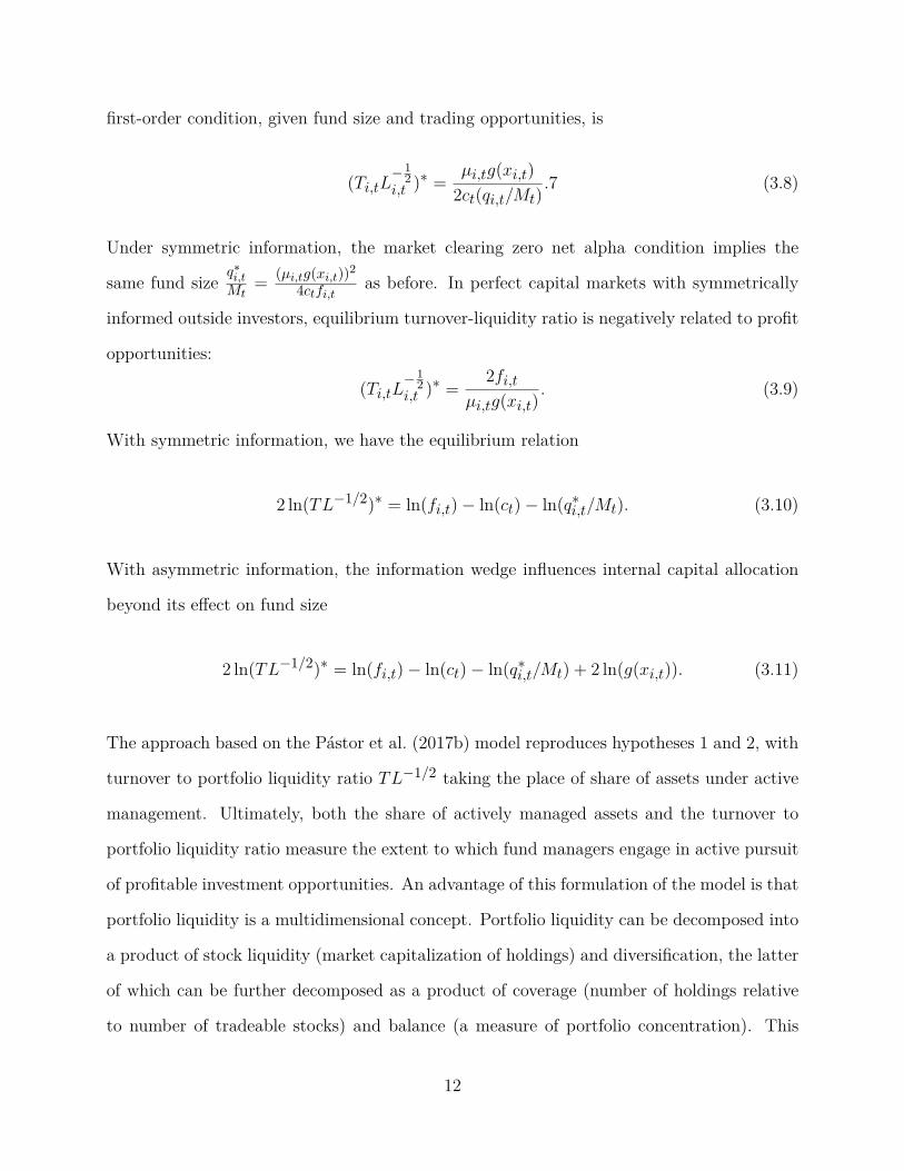
first-order condition, given fund size and trading opportunities, is

(Ti,tL−1

2i,t )∗ =

µi,tg(xi,t)2ct(qi,t/Mt)

.7 (3.8)

Under symmetric information, the market clearing zero net alpha condition implies the

same fund size q∗i,tMt

= (µi,tg(xi,t))2

4ctfi,t as before. In perfect capital markets with symmetrically

informed outside investors, equilibrium turnover-liquidity ratio is negatively related to profit

opportunities:

(Ti,tL−1

2i,t )∗ =

2fi,tµi,tg(xi,t)

. (3.9)

With symmetric information, we have the equilibrium relation

2 ln(TL−1/2)∗ = ln(fi,t) − ln(ct) − ln(q∗i,t/Mt). (3.10)

With asymmetric information, the information wedge influences internal capital allocation

beyond its effect on fund size

2 ln(TL−1/2)∗ = ln(fi,t) − ln(ct) − ln(q∗i,t/Mt) + 2 ln(g(xi,t)). (3.11)

The approach based on the Pástor et al. (2017b) model reproduces hypotheses 1 and 2, with

turnover to portfolio liquidity ratio TL−1/2 taking the place of share of assets under active

management. Ultimately, both the share of actively managed assets and the turnover to

portfolio liquidity ratio measure the extent to which fund managers engage in active pursuit

of profitable investment opportunities. An advantage of this formulation of the model is that

portfolio liquidity is a multidimensional concept. Portfolio liquidity can be decomposed into

a product of stock liquidity (market capitalization of holdings) and diversification, the latter

of which can be further decomposed as a product of coverage (number of holdings relative

to number of tradeable stocks) and balance (a measure of portfolio concentration). This

12

framework allows the researcher to study each dimension, potentially allowing for a richer

characterization of fund behavior.

13

CHAPTER 4

DATA

I build my dataset around two main sources. From the CRSP Survivor-Bias-Free US Mutual

Fund database I obtain share class level information on returns, net asset values, expense

ratios, TNA, fund turnover, first offer date, name, various fund objective classifications,

and flags indicating index fund and ETF/ETN status. The CRSP Mutual Fund database

includes data starting from January 1960. From the Thomson Reuters S12 database, I

procure fund-level share holdings and additional information on fund investment objectives.

Thomson’s predecessor first compiled holdings data in March 1980, subsequent to which

consistent holdings reports are available.1 I supplement these two main sources by security-

level data on prices and shares outstanding from CRSP, monthly return factors from Ken

French’s data library,2 and active share (Cremers and Petajisto, 2009; Petajisto, 2013) from

Antti Petajisto’s website.3

TNA is typically only available at the quarterly or semi-annual frequency in the CRSP files

before 1991 (Figure A.1). I interpolate missing TNA by assuming zero net flows. For up

to one year following the most recent non-missing TNA value, I replace missing time t + 1

values of TNA as TNAt+1 = TNAt(1 + rt+1), where r corresponds to net returns.

I link CRSP mutual fund data to Thomson holdings data using MFLINKS (Wermers, 2000;

Cao and Xue, 2015), currently available until 2016.4 Since CRSP data are at the share

class level, at each date I aggregate variables to the portfolio level by taking the lagged

1. The 1980 March vintage includes a smattering of holding reports dated between 1979 December and1980 February. For a detailed discussion of vintage dates vs report dates, see Appendix F. In the analysis, Ionly consider holdings reported during or after 1980 March.

2. http://mba.tuck.dartmouth.edu/pages/faculty/ken.french/data_library.html

3. http://www.petajisto.net/data.html. This dataset also includes the identity of the benchmark againstwhich active share is calculated.

4. Zhu (2017) shows that Thomson’s coverage of new share classes deteriorates after 2008. In the Ap-pendix, I replicate analyses using data up to 2008. The results remain similar.

14

http://mba.tuck.dartmouth.edu/pages/faculty/ken.french/data_library.html

http://www.petajisto.net/data.html

TNA-weighted average of returns, expense ratio, turnover, and summing up TNA. Following

Pástor et al. (2017a), I winsorize turnover at the 1% level. The final sample is a fund-month

level panel spanning March 1980-December 2016.

4.1 Fund Selection

My aim is to study competition among long-only, general purpose actively managed U.S.

domestic equity funds. I purge my sample of fixed income and “balanced” funds, money

market funds, international funds, passive index funds, specialist long-short and sector funds,

as well as target date funds. I use a variety of filters, based partially on previous research,

and developed through a process of case-by-case inspection.5 The filters primarily rely on

a combination of various investment objective classifications, as well as exclusions based on

fund names. I describe the fund selection algorithm in Appendix F in precise detail, and

outline it below.

Since my analysis relies on within-fund variation, I construct filters at the fund level. I

exclude all funds ever classified as International, Municipal Bonds, Bond & Preferred, Bal-

anced, or Metals by Thomson investment objective codes. I exclude a fund if any of its share

classes are ever assigned a policy code contrary to a long-only equity strategy,6 assigned a

CRSP objective code indicating sector fund or fixed income fund, flagged as an index fund, or

have names indicative of index funds, target date funds, international funds, or tax managed

funds. I exclude funds that are identified over 25% of the time as foreign equity by CRSP

objective codes. This means that my dataset includes a handful of funds that transition to

investing a portion of their assets in foreign markets.

5. The skeleton of my filtering algorithm is the scheme described in Kacperczyk et al. (2008). However,inspection of the fund universe resulting from my implementation of this scheme indicated a significantnumber of remaining international funds, sector funds, etc. This observation led me to add a number ofadditional filters.

6. Including codes corresponding to the following classifications: Balanced, Bonds & Preferred Stock,Bonds, Canadian & International, Leverage and/or Short Selling, Leases, Government Securities, MoneyMarket, Preferred Stock, Sector/Highly Speculative, and various Tax Free.

15

In addition to the exclusion screens, I use objective codes to constructively identify actively

managed domestic equity funds. I first use Lipper Class, including funds if any of their share

classes are ever assigned a classification consistent with a domestic equity strategy.7 If Lipper

Class is not available, I consider Strategic Insights Objective Codes,8 and if neither Lipper

Class nor Strategic Insights Objective Codes are available, then Weisenberger Objective

Codes.9 I exclude fund-month observations with expense ratio below 0.1% as these are

unlikely to correspond to active funds. To lessen the impact of incubation bias (Evans,

2000), I drop fund-month observations with lagged TNA below $15m in 2017 dollars.

4.2 Portfolio Weights

Although Thomson compiles updates on portfolio holdings at regular quarterly intervals,

these updates do not exclusively consist of quarter-end reports of fund holdings. As shown

in Figure A.2, a significant proportion of reports are dated outside of quarter-end months.

I index each fund i’s most recent reporting period at month t as tir, yielding a many-to-one

mapping from month t to report date tir for each fund. I consider portfolio holdings as stale

beyond six months. Therefore, there are at most six distinct values of t that correspond to

each tir. Let Qh,i,tir denote the number of split adjusted shares of security h held by fund i

at reporting date tir, Ph,t the split adjusted price of security h at month t, and θi,tirthe set

of securities classified as U.S. common equity by CRSP in fund i’s portfolio reported at tir.

7. Included classes are: Equity Income Funds, Growth Funds, Large-Cap Core Funds, Large-Cap GrowthFunds, Large-Cap Value Funds, Mid-Cap Core Funds, Mid-Cap Growth Funds, Mid-Cap Value Funds,Multi-Cap Core Funds, Multi-Cap Growth Funds, Multi-Cap Value Funds, Small-Cap Core Funds, Small-Cap Growth Funds, and Small-Cap Value Funds.

8. Included codes correspond to Equity USA Aggressive Growth, Equity USA Midcaps, Equity USAGrowth & Income, Equity USA Growth, Equity USA Income & Growth, or Equity USA Small Companies.

9. Included codes correspond to Growth, Growth-Income, Growth and Current Income, Long-TermGrowth, Maximum Capital Gains, or Small Capitalization Growth.

16

I define the weight of security h in fund i’s portfolio at time t as

wh,i,t =Qh,i,tir

Ph,t∑h∈θ

i,tirQh,i,tir

Ph,t. (4.1)

Stacking the portfolio weights for each fund, denote the vector of portfolio weights by wi,t.

4.3 CompetitorSize

For each fund, I calculate CompetitorSize as the sum of all other funds’ size, weighted by

the cosine similarity between the funds’ stock capitalization adjusted portfolio weights. I

cap adjust portfolio weights, as cross-holding a given security is more informative about fund

similarity when the market capitalization of the cross-held security is small (Cohen et al.,

2005). I define capitalization adjusted weights as portfolio weights scaled by the inverse of

the security’s weight in the market portfolio:

w̃h,i,t =wh,i,twh,m,t

, (4.2)

where wh,m,t is the weight in the market portfolio. I stack adjusted weights into vectors,

denoted w̃i,t.

Define similarity weights ψki,j,t for fund i with respect to fund j as the cosine similarity

between their vectors of capitalization adjusted portfolio weights:10

ψi,j,t =w̃i,t · w̃j,t

∥w̃i,t∥∥w̃j,t∥. (4.3)

CompetitorSize is the similarity-weighted size of all other funds in the industry as of the

10. Cosine similarity represents the cosine of the angle between the funds’ adjusted portfolio weight vectors.It is widely used in machine learning, and is used in finance academia with increasing frequency. For example,both Blocher (2016) and Hoberg et al. (2018) use cosine similarity of holdings to measure fund similarity.Cohen et al. (2016) use cosine similarity to measure similarity between company 10-K and 10-Q filings.

17

fund’s most recent reporting date:

CompetitorSizei,t =∑j ̸=i

ψi,j,tirFundSizej,tir

, (4.4)

where

FundSizej,tir=

TNAj,tirTotalMktCaptir

, (4.5)

with TotalMktCap representing the total market capitalization of all U.S. domestic equity

in the CRSP universe. CompetitorSizei,t is invariant between each fund’s reporting dates.11

As a reference point, I calculate the total size of the actively managed mutual fund industry

following Pástor et al. (2015) as IndustrySize = ∑j FundSizej,t.

4.4 Portfolio Liquidity

I calculate portfolio liquidity and its components (stock liquidity, diversification, coverage,

and balance) according to Pástor et al. (2017b), constructing them with respect to the CRSP

U.S. domestic equity universe.

4.5 Summary Statistics

Since my analysis relies on within-fund variation, I require each fund to have at least twelve

months of non-missing observations of both returns and CompetitorSize to be included in

the estimation sample. My sample runs from March 1980 to December 2016, and includes

2,553 distinct funds. Table B.1 reports summary statistics.

The time series of the cross-sectional average competitor size and aggregate industry size

are closely related (Figure B.1). Figure 4.1 presents histograms of the distribution of

11. The results remain virtually unchanged if I allow the measure to reflect within report date changesin the implied buy-and-hold portfolio weights and the size of competing funds by calculating it as∑

j ̸=i ψi,j,tFundSizej,t.

18

0

50

100

150

200

0.00 0.01 0.02

CompetitorSize

Den

sity

Unconditional distribution

0

100

200

300

−0.01 0.00 0.01 0.02

CompetitorSize

Den

sity

Within−fund distribution

Figure 4.1. Histograms of CompetitorSize. The left panel illustrates the variable’s uncon-ditional distribution. The right panel shows the distribution after demeaning fund-by-fund.

CompetitorSize. The unconditional distribution is right skewed, as shown in the left panel.

This is to be expected, as CompetitorSize is a weighted sum of the highly skewed FundSize.

The distribution is less dispersed once the variable is demeaned fund-by-fund, but exhibits

sufficient variation for meaningful within-fund analysis.

4.6 Correlations

Panel A of Table B.2 presents unconditional pairwise correlations between variables, while

Panel B presents within-fund pairwise correlations. CompetitorSize is positively corre-

lated with IndustrySize both unconditionally (ρ = 0.38) and at the fund level (ρ = 0.60).

The residual within-fund variation in CompetitorSize with respect to IndustrySize reflects

heterogenous dynamics in competitor size across funds pursuing different investment strate-

gies.12

There is a small but negative correlation between CompetitorSize and risk adjusted gross re-

turns, both unconditionally (ρ = -0.02) and within-fund (ρ = -0.03). CompetitorSize tends

12. This residual variation is useful for identification, as the time series correlation between IndustrySizeand a linear time trend is ρ = 0.92, making industry level decreasing returns to scale hard to distinguishfrom simple trends in the data.

19

to increase over each fund’s lifetime. The within-fund correlation between CompetitorSize

and FundAge is ρ = 0.51. The unconditional correlation is markedly lower (ρ = 0.10),

indicating that new funds begin their operations exploiting relatively lightly contested in-

vestment opportunities. CompetitorSize is highly correlated with portfolio liquidity both

unconditionally (ρ = 0.75) and within-fund (ρ = 0.63), evidence that more liquid market

segments are capable of absorbing higher levels of active investment. Consistent with the

joint determination of fund size, portfolio liquidity, turnover, and expense ratios in Pástor

et al. (2017b), larger funds tend to be more liquid, trade less, and charge lower fees.

20

CHAPTER 5

CAPITAL ALLOCATION AND COMPETITOR SCALE

5.1 Decreasing Returns to Competitor Scale

I develop empirical tests of hypotheses 1 and 2 using competitor scale as the external con-

straint on the profitability of investment opportunities. This choice is motivated by both the

extant literature and novel evidence from my sample. Pástor et al. (2015) give time series

evidence that funds suffer from decreasing returns to aggregate industry scale. In recent

work, Hoberg et al. (2018) provide cross-sectional evidence of decreasing profitability due to

inter-fund competition. In Appendix C, I relate competitor scale to fund performance, using

only within-fund variation. My results are consistent with decreasing returns to competitor

scale. The following is a brief summary.

• A one standard deviation increase in competitor size is associated with a 76bp decrease

in annual Fama-French three factor adjusted returns.

• Competitor size subsumes the negative effect of aggregate industry size in a head-to-

head horse race.

• The negative impact of competitor size is smaller for funds which on average hold

more liquid portfolios. This is consistent with liquidity constraints as the channel for

decreasing returns to competitor scale.

• The negative impact of competitor size is smaller when funds tilt toward more liquid

portfolios. This suggests that increased portfolio liquidity shelters funds from the

pernicious effects of decreasing returns to scale.

• Holding skill fixed, funds make more when they hold less liquid portfolios. One inter-

pretation is that funds increase portfolio concentration when they perceive favorable

investment opportunities.

21

5.2 Empirical Strategy

Motivated by decreasing returns to competitor scale, I parametrize the profitability of a

fund’s time t investment opportunities as

g(xi,t) = CompetitorSize−γi,t . (5.1)

This is a sensible choice in that alpha before transaction costs is a decreasing function of

competitor scale, asymptoting to zero as the market approaches perfect competition.

The fraction of assets under active management in Berk and Green (2004) is similar in spirit

to active share (denoted AS) from Cremers and Petajisto (2009), Petajisto (2013).1 The

Pástor et al. (2017b) portfolio choice maps directly into data on turnover and fund hold-

ings. Therefore, letting yi,t ∈ {ASi,t,(TL−1/2

)i,t

}, the equilibrium relation (with potential

information asymmetry) in equation (3.7) implies the regression model

ln(yi,t) = αt + η1 ln(FundSizei,t) + η2 ln(fi,t) + γ ln(CompetitorSizei,t) + εi,t. (5.2)

Outcome y and CompetitorSize are both calculated based on the same portfolio weights. To

ensure that my findings are not an artifact of measurement, I consider quarter end holding

reports only, and calculate the log change in CompetitorSize, holding constant previous

quarter-end similarity weights. That is, let t be quarter end dates, and define

∆CSi,t = ln

∑j ̸=i

ψi,j,t−1FundSizej,t

− ln

∑j ̸=i

ψi,j,t−1FundSizej,t−1

. (5.3)

1. Cremers (2017) shows that for funds that do not short or use leverage, active share is equal to oneminus the sum of holdings that overlap with the benchmark. Letting J be the set of stocks held by the fundand B the set of stocks in the benchmark b, we have

ActiveShare = 1 −∑

j∈J∩B

min{wi,j , wb,j}.

22

Note that the fund’s change in capital allocation from t− 1 to t has no mechanical effect on

∆CS, as it is determined only by changes in other fund size, holding similarity fixed.

I then estimate equation (5.2) in quarterly first differences as

∆ ln(yi,t) = αt + η1∆ ln(FundSizei,t) + η2∆ ln(fi,t) + γ∆CSi,t + ∆εi,t. (5.4)

I double cluster standard errors by fund and date × portfolio group.2 Under the hypothesis

of symmetrically informed outside investors, γ = 0. Under the joint hypothesis of decreasing

returns to competitor scale and asymmetric information, γ < 0. I also perform the anal-

ysis separating out portfolio liquidity and its components. In these regressions, the joint

hypothesis of decreasing returns to competitor scale and asymmetric information implies

γ > 0.

5.3 Results

Table 5.1 presents results from empirical tests evaluating hypothesis 1 against hypothesis

2. The statistically significant coefficients on ∆CS provide a rejection of the hypothesis

that managers and outside investors are symmetrically informed of investment opportunities

captured by changes in the scale of competing funds.

The results are consistent with managers reacting optimally to decreasing returns to own and

competitor scale by scaling back active management. A one percent increase in competitor

size is associated with a 4bp decrease in active share, and a 52bp decrease in the turnover

to portfolio liquidity ratio. Since turnover is reported on a fiscal year basis, the estimated

negative relation between competitor scale and turnover-liquidity ratio is likely driven by

portfolio liquidity: a one percent increase in competitor size is associated with a 79bp increase

2. Fund portfolios are grouped using k-means cluster analysis of raw portfolio weights. Each month,this process constructs k = 10 archetypal portfolios (serving as cluster centers). These model portfoliosare constructed and then funds are assigned to each such that the sum of squared differences between theweights of fund portfolios and their assigned model portfolio is minimized.

23

Table 5.1Capital Allocation and Competitor Scale

Observations are at the fund-quarter level, from 1980-2016. ∆ denotes first differences. Dependent variables are noted inthe column headers. AS is active share relative to self-declared benchmarks from Petajisto (2013), covering years 1980-2009.T is turnover; L, S, D, C, and B are respectively portfolio liquidity, stock liquidity, diversification, coverage, and balance,as defined in Pástor et al. (2017b). ∆CSi,t = ln

(∑j ̸=i


)− ln

(∑j ̸=i


)is the

change in log competitor size, holding previous quarter end similarity weights fixed. Standard errors are double clusteredby fund and portfolio group × quarter, and reported in parentheses. Asterisks denote statistical significance: *** p <0.01,** p <0.05, * p <0.1.

Dep. Var.: ∆ ln(AS) ∆ ln(TL−1/2) ∆ ln(L) ∆ ln(S) ∆ ln(D) ∆ ln(C) ∆ ln(B)

∆CS -0.045*** -0.521*** 0.794*** 0.624*** 0.599*** 0.179*** 0.515***(0.016) (0.056) (0.079) (0.077) (0.064) (0.029) (0.058)

∆ ln(FundSize) -0.016*** -0.111*** 0.184*** 0.101*** 0.163*** 0.098*** 0.101***(0.002) (0.012) (0.013) (0.010) (0.011) (0.007) (0.009)

∆ ln(f) -0.021 0.037 0.039* -0.011 0.053** 0.029** 0.034*(0.017) (0.027) (0.021) (0.019) (0.022) (0.012) (0.019)

∆ ln(T ) -0.005 -0.004 -0.003 0.003 -0.006*(0.004) (0.003) (0.004) (0.002) (0.003)

∆ ln(D) -0.355***(0.019)

∆ ln(S) -0.632*** -0.194*** -0.539***(0.017) (0.014) (0.022)

∆ ln(B) -0.126***(0.011)

∆ ln(C) -0.293***(0.023)

Fixed Effects• Quarter Yes Yes Yes Yes Yes Yes YesObservations 35,285 57,240 57,240 57,240 57,240 57,240 57,240R2 0.025 0.020 0.047 0.252 0.245 0.098 0.219R2 (proj. model) 0.004 0.007 0.031 0.233 0.231 0.077 0.209

in portfolio liquidity. Increases in competitor scale are also associated with statistically

significant increases in each component of portfolio liquidity. As the scale of their competitors

increase, funds tend to increase the stock liquidity and diversification of their portfolios,

including coverage and balance.

Pástor et al. (2017b) argue that unit trading costs might vary by fund segment, implying a

model with segment × time fixed effects. To accommodate segment level variation in trading

costs, I repeat the analysis with benchmark × quarter fixed effects in Table D.2. The results

remain similar. The results are also similar if, following Zhu (2017), I restrict the estimation

data to pre-2008 observations (Tables D.1, D.3).

24

CHAPTER 6

EVIDENCE FROM THE 2003 MUTUAL FUND SCANDAL

In September 2003, the New York Attorney General’s office launched investigations into

several high-profile mutual fund families for illegal trading practices. Families were charged

with allowing favored clients to trade fund shares at stale prices at the expense of ordinary

shareholders (Houge and Wellman, 2005; Zitzewitz, 2006). By the end of October 2004,

official investigations had been announced against a total of twenty-five mutual fund families.

Houge and Wellman (2005) and McCabe (2008) argue that investors penalized tainted funds

with large outflows. This is borne out in my data. Figure 6.1 plots mean net flows by scandal

involvement.1

The two series track each other closely in the two years prior to the scandal, and diverge

abruptly in September 2003. The wedge between the two groups persists until the end

of 2006, coincident with the final settlements negotiated with the Securities and Exchange

Commission (Zitzewitz, 2009).2

I conclude that the scandal caused a significant reallocation of resources away from tainted

1. I follow Table 1 of Houge and Wellman (2005) for classifying fund families embroiled in the scandal.The following is the list of fund families tainted by the scandal by month of the news date of investigation.September 2003: Alliance Bernstein, Franklin Templeton, Gabelli, Janus, Nations, One Group, Putnam,Strong. October 2003: Alger, Federated. November 2003: Excelsior/US Trust, Fremont, Loomis Sayles,PBHG. December 2003: AIM/Invesco, MFS, Heartland. January 2004: Columbia, Scudder, Seligman.February 2004: PIMCO. March 2004: ING, RS. August 2004: Evergreen. October 2004: Sentinel.I identify funds belonging to these families as of August 2003 in my sample based on the share class names inthe CRSP mutual fund dataset. I classify 289 of the 1,461 funds in my sample in August 2003 with existingholdings and gross returns as members of future tainted families. Table E.1 presents a snapshot of summarystatistics as of August 2003 by future scandal involvement. Tainted funds are slightly older, larger, and havehigher turnover to portfolio liquidity and expense ratios.

2. The difference is statistically significant. Using a two year pre- and post-scandal window of observations,I estimate a regression of the form

flowi,t = αi + αt + γPostNewsi,t +12∑

τ=1Ri,t−τ + εi,t,

where PostNewsi,t is an indicator for tainted funds after news of their involvement in the scandal break. Ifind γ =-11.1% per year, with t-statistic of -5.2 (clustered by fund and portfolio group × month).

25

−0.01

0.00

0.01

0.02

2002 2004 2006

Date

Mon

thly

flow

s in

%

Involved in scandal Not involved in scandal

0.00

0.05

0.10

0.15

Sep

03

Dec

03

Mar

04

Aug

04

Oct

04

News date of investigation

Invo

lved

fund

siz

e

Figure 6.1. Flows and assets by scandal involvement. The left panel plots mean monthlynet flows. The vertical line corresponds to August 2003, the month before the announcementof the first investigations. The right panel shows the total net assets of funds coming underinvestigation in a given month, as a fraction of the total net assets managed by all funds inmy sample.

funds. Unless flows are perfectly offsetting, this shift causes a relative reduction in the

competitor size of the most similar funds. Under decreasing returns to competitor scale, we

would expect the investment opportunities of these funds to improve in relative terms, leading

them to differentially expand active management and earn higher risk-adjusted returns.

I test these hypotheses by comparing untainted funds with differential pre-scandal similarity

to prospective scandal funds. I discard tainted funds as the internal upheaval following the

scandal likely had a direct impact on their performance and investment behavior.3 I take

two approaches. The first is a straightforward difference-in-differences-style comparison of

fund outcomes before and after the scandal as a function of their pre-scandal exposure to

tainted funds. The second approach links fund outcomes directly to variation in competitor

size attributable to abnormal flows among tainted funds. I first present an analysis on fund

capital allocation, followed by an analysis of fund performance.

3. In the aftermath of the investigations, several executives stepped down, and a number of portfoliomanagers were fired. Perhaps the highest profile casualty of the scandal was Richard S. Strong, founder ofStrong Capital Management, who resigned in December 2003. Strong would go on to pay $60 million insettlements and be barred from the industry. Strong Capital itself was acquired by Wells Fargo in 2004.

26

6.1 Before and After Analysis

I relate fund-by-fund differences in pre-scandal [2003m8 − W , 2003m8] and post-scandal

[2004m11, 2004m11 + W ] outcomes to pre-scandal exposure to competition from tainted

funds. I consider W ∈ {1, 2} year windows. For a fund to be included in the estimation

sample, it must have available holdings information for August 2003, and I must observe it

both in the pre- and the post-scandal period.

I measure pre-scandal exposure as the proportion of competitor size attributable to prospec-

tive tainted funds as of August 2003. Let Φ denote the set of funds that belong to families

later investigated, and define

ScandalExposurei =∑j∈Φ ψi,j,2003m8FundSizej,2003m8∑j ̸=i ψi,j,2003m8FundSizej,2003m8

. (6.1)

On average, 22% of untainted funds’ competitor size is due to tainted fund families. Exposure

ranges from 7% to 42%, with lower quartile 20% and upper quartile 26%.

To present interpretable summary statistics, I sort funds into high and low exposure groups

depending on whether their ScandalExposure is above or below the cross-sectional median.

Table E.2 gives a snapshot taken in August 2003. High exposure funds are slightly smaller,

have higher turnover to portfolio liquidity ratios, expense ratios, CompetitorSize, and worse

performance. Fund age is almost identical across the two groups, limiting the plausibility of

life cycle effects as an explanation for differences in outcome paths.

Figure 6.2 summarizes the identifying variation in the data. I plot the groupwise cross-

sectional mean of within-fund deviations for log competitor size, log active share, log port-

folio liquidity, and log turnover. The differential impact of the scandal across groups is

identified by the difference in the pre- and post-scandal period wedges between the series.

The CompetitorSize of the low exposure group overall trends upward, despite a small dip in

the middle of the scandal period. The CompetitorSize of high exposure funds drops more

27

−0.2

−0.1

0.0

0.1

2002 2004 2006

Date

ln(C

.S)

High exposure Low exposure

ln(CompetitorSize)

−0.02

0.00

0.02

0.04

2002 2003 2004 2005 2006

Date

ln(A

S)


ln(AS)

−20

−10

0

10

20

2002 2004 2006

Date

Rhi

ghF

F3

−R

low

FF

3

RFF3

−0.1

0.0

0.1

2002 2004 2006

Date

ln(L

)


ln(L)

−0.05

0.00

0.05

0.10

2002 2004 2006

Date

ln(T

)


ln(T)

−0.1

0.0

0.1

0.2

2002 2004 2006

Date

ln(T

L)


ln(TL−12)

Figure 6.2. Untainted fund outcomes by ScandalExposure. Funds are sorted into highand low exposure groups depending on whether their ScandalExposure is above or belowthe cross-sectional median. The RFF3 panel plots the difference between the cross-sectionalmeans of the within-fund deviations of three factor adjusted gross returns across high andlow exposure groups. Other panels plot the cross-sectional groupwise means of respectivevariables’ deviations from within-fund means. The ln(AS) panel plots only quarter-endmonths as the variable is seldom reported within quarter. The shaded area corresponds tothe scandal period Sep 2003-Oct 2004.

28

substantively during the scandal, and remains flat for almost a year after the end of the

scandal period. The historical accident of scandal-related outflows at involved funds appear

to have insulated their closest competitors from contemporaneous increases in the aggregate

size of the industry.

The active share of low exposure funds is essentially flat during this period, whereas the active

share of high exposure funds is flat in the pre-period, and then increases steadily during and

after the scandal. The portfolio liquidity of high and low exposure funds exhibit broadly

parallel increases in the pre-period. Following the scandal, the portfolio liquidity of low

exposure funds continues to increase, whereas the portfolio liquidity of high exposure funds

decreases during the scandal period and then levels off. These phenomena are consistent

with high exposure funds responding to improved prospects by shifting resources away from

the benchmark, tilting toward less liquid, more concentrated portfolios.

The patterns in turnover do not lend themselves to easy interpretation. The turnover of low

exposure funds trends downward in the first half of the sample, and then swings upward

during the second half, whereas the turnover of high exposure funds remains relatively flat,

with an upward blip during the year ending in Sep 2003. Note that funds only report turnover

once a year, as a cumulative measure that applies for the most recently concluded fiscal year.

This is in contrast to holdings-based measures such as active share or portfolio liquidity,

which can typically be calculated quarterly, based on unambiguously timed snapshots of

portfolio holdings. The poor measurement of turnover’s timing makes it a less suitable

outcome variable for this analysis, which is designed to exploit tightly timed differences in

fund outcomes as a function of exposure to competition by tainted funds.

Returns are highly volatile, which presents a challenge for providing a visual comparison of

trends across groups. To compare relative fund performance before and after the scandal, for

each month I plot the difference between high and low exposure groups’ mean within-fund

three factor adjusted returns. High exposure funds relatively underperform low exposure

29

funds in the pre-scandal period, are essentially even during the scandal, and enjoy a string

of relative outperformance in the year after the end of the scandal period. The differential

relative before and after performance of the two groups is consistent with decreasing returns

to competitor scale.

To formally test for differential differences in before and after outcomes as a function of ex

ante exposure to competition from prospective scandal funds, I perform regressions of the

form

yi,t = αi + αt + γ (It × ScandalExposurei) + Xi,tΓ + εi,t, (6.2)

where Xi,t includes log fund size and expense ratio, as dictated by theory. In the regression,

exposure is a continuous variable. I double cluster standard errors by fund and portfolio

group × time. I normalize ScandalExposure by its interquartile range (≈ 6%).

Table 6.1 presents results. The one (two) year window estimate implies a statistically sig-

nificant 6.4% (3.4%) post-scandal reduction in CompetitorSize for untainted funds at the

75th percentile of ScandalExposure relative to untainted funds at the 25th percentile of

ScandalExposure. The same difference in ScandalExposure is associated with a statis-

tically significant 2.6% (3.4%) relative increase in active share. The increase in turnover-

liquidity ratio is positive but not statistically significant (1.9% at the one year horizon

and 1.0% at the two year horizon). The weak response is due to turnover: increasing

ScandalExposure from its 25th to its 75th percentile is associated with a highly significant

10.1% (10.1%) decrease in portfolio liquidity at the one (two) year horizon. Examining

each component of portfolio liquidity separately reveals a shift toward lower portfolio liquid-

ity among high exposure funds on all dimensions, as evidenced by statistically significant,

negative coefficients associated with I × ScanEx for all outcomes except balance.

30

Table 6.1Capital Allocation and the Scandal: Before and After Analysis

Dependent variables are identified in the column headers. ln(C.S.) is an abbreviation for ln(CompetitorSize). Observationsare at the fund-report date level, including only funds not directly involved in the scandal over the period {(2003m8 −W, 2003m8], [2004m11, 2004m11 + W )}, where W corresponds to the number of years specified in the panel headers. I ×ScanEx is the interaction of ScandalExposure (normalized by its interquartile range) and an indicator for the post-scandalperiod. Standard errors are double clustered by fund and portfolio group × date, and reported in parentheses. Asterisksdenote statistical significance: *** p <0.01, ** p <0.05, * p <0.1.

Dep. Var.: ln(C.S.) ln(AS) ln(TL−1/2) ln(L) ln(S) ln(D) ln(C) ln(B)

Panel A: 1 year window

I × ScanEx -0.064*** 0.026*** 0.019 -0.101*** -0.095*** -0.049** -0.026* -0.026(0.019) (0.006) (0.033) (0.024) (0.017) (0.022) (0.014) (0.017)

ln(FundSize) 0.130*** -0.013** -0.163*** 0.171*** 0.083*** 0.139*** 0.072*** 0.077***(0.021) (0.007) (0.032) (0.026) (0.014) (0.025) (0.020) (0.018)

ln(f) -0.004 -0.015 0.073 0.015 -0.067 0.065 0.096 -0.024(0.098) (0.029) (0.141) (0.115) (0.076) (0.106) (0.076) (0.077)

ln(T ) -0.079*** -0.065*** -0.045* 0.017 -0.064***(0.027) (0.016) (0.025) (0.015) (0.019)

ln(D) -0.228***(0.029)

ln(S) -0.450*** -0.243*** -0.238***(0.050) (0.041) (0.050)

ln(B) -0.056*(0.034)

ln(C) -0.083*(0.048)

Fixed Effects• Fund Yes Yes Yes Yes Yes Yes Yes Yes• Time Yes Yes Yes Yes Yes Yes Yes YesObservations 7,073 6,067 6,893 6,893 6,893 6,893 6,893 6,893R2 0.927 0.914 0.896 0.962 0.987 0.941 0.942 0.892R2 (proj. model) 0.052 0.022 0.023 0.076 0.156 0.121 0.083 0.062

Panel B: 2 year window

I × ScanEx -0.034* 0.029*** 0.010 -0.101*** -0.105*** -0.040* -0.032** -0.011(0.020) (0.006) (0.033) (0.025) (0.018) (0.022) (0.015) (0.016)

ln(FundSize) 0.148*** -0.018*** -0.200*** 0.183*** 0.088*** 0.147*** 0.073*** 0.084***(0.017) (0.006) (0.026) (0.022) (0.014) (0.021) (0.016) (0.015)

ln(f) -0.098 0.005 0.171 -0.074 -0.169** 0.039 0.104 -0.061(0.073) (0.027) (0.126) (0.109) (0.077) (0.091) (0.072) (0.072)

ln(T ) -0.063*** -0.065*** -0.025 0.023 -0.049***(0.024) (0.014) (0.022) (0.014) (0.015)

ln(D) -0.216***(0.022)

ln(S) -0.425*** -0.217*** -0.236***(0.036) (0.033) (0.040)

ln(B) -0.055**(0.024)

ln(C) -0.077**(0.033)


The main concern with identification based on comparing pre- and post-event periods across

31

groups is that the measured effect might be the manifestation of favorable trends across the

groups in the pre-period. I test for differential trends in the pre-period as a function of

ScandalExposure by estimating the regression

yi,t = αi + αt + γ (t× ScandalExposurei) + Xi,tΓ + εi,t, (6.3)

where t is a linear time trend and Xi,t includes the usual controls. I estimate this regression

on pre-period observations. Differential pre-trends by ScandalExposure would be a concern

if the coefficient on the trend interaction was statistically significant and of the same sign as

the corresponding interaction coefficient in Table 6.1. Results from these specifications fail

to reject the null hypothesis of no differential trends in the pre-period (Table E.3), with the

exception of a slight favorable trend in the portfolio-liquidity ratio at the two year horizon

due to the patterns in turnover seen in Figure 6.2.

6.2 Linking CompetitorSize Directly to Abnormal Flows

The analysis above does not explicitly model untainted fund outcomes as a function of the

relevant shock to competitor scale, namely, the abnormal outflows from competing tainted

funds. I aim to fill this gap in the following. I first estimate outflows at tainted funds

attributable to the scandal. In turn, I relate untainted fund outcomes to variation in com-

petitor size explained by abnormal tainted competitor outflows.

I use a linear model to decompose variation in fund flows between the effects of the scandal

and baseline variation. I pool tainted and untainted funds in the two year window surround-

ing the scandal period, consisting of observations from September 2001 to October 2006.

Consider scandal funds as being from the same cohort d if news of investigation into their

trading practices broke in month d. Denote the cohort of fund j as j(d). Let It≥j(d) be an

indicator for post investigation months for fund j, and define Id,t as cohort × time dummy

32

−0.02

−0.01

0.00

2004 2005 2006

Date

β j(d

) t

0

1

2

3

4

2004 2005 2006

Date

Sca

ndal

Out

Flo

w ×

1000

0 p75

p50

p25

Figure 6.3. Estimated abnormal outflows from scandal funds. The left panel shows the cross-sectional mean coefficient on post-scandal cohort × time fixed effects from equation (6.4).The right panel shows the time series of cross-sectional percentiles of ScandalOutF low acrossuntainted funds.

variables. I regress flows on the full set of post-investigation cohort × time indicators,

controlling for fund and time fixed effects:

flowj,t = αj + αt + βj(d),t

(It≥j(d)Ij(d),t

)+ εj,t. (6.4)

I interpret the betas as the path of abnormal flows attributable to the scandal for each cohort

of tainted funds. I cumulate abnormal flows for each fund at each post-scandal date as

f̂j,t =t∏

τ≥j(d)

(1 + β̂j(d),t

)− 1. (6.5)

I construct ScandalOutF low for untainted fund i as the similarity- and size-weighted cumu-

lative abnormal negative net flow among tainted funds j ∈ Φ:

ScandalOutF lowi,t = −∑j∈Φ

ψi,j,2003m8(f̂j,tFundSizej,2003m8

). (6.6)

One can interpret ScandalOutF low as the expected decrease in CompetitorSize for un-

tainted funds due to scandal-related outflows among tainted funds, given the pattern of fund

similarities immediately preceding the scandal.

33

Figure 6.3 plots time series characteristics of abnormal flows and ScandalOutF low. Abnor-

mal flows are most negative in the immediate aftermath of the announcement of the first

investigations, and gradually converge to zero near the end of 2006. This pattern maps

into almost linearly increasing cumulative outflows in the first two years after the scandal,

reflected in the observed pattern in ScandaOutF low. Importantly for identifying differen-

tial spillover effects of the scandal, total predicted outflows at competing tainted funds vary

substantially in the cross-section.

This line of analysis at its core relies on differences in pre- and post-scandal outcomes among

untainted funds as a function of post-scandal outflows among competing tainted funds. To

illustrate the identifying variation, I sort funds into high and low outflow groups based

whether their fund-level mean ScandalOutF low is above or below the median. I then plot

cross-sectional mean within-fund demeaned outcomes for each group in Figure 6.4. The

patterns are similar to Figure 6.2: the high outflow group exhibits a relative post-scandal

decline in competitor size and portfolio liquidity, and an increase in active share. The two

groups exhibit differential trends in turnover before 2003, but there is convergence before

the scandal, and a relative increase in the turnover of the high group around the second half

of 2004.

I formally test the link between tainted fund flows and untainted fund outcomes through the

regression specification

yi,t = αi + αt + γScandalOutF lowi,t + Xi,tΓ + εi,t, (6.7)

where Xi,t includes log size and expense ratio. To make γ readily interpretable, I normalize

ScandalOutF low by its interquartile range.

Table 6.2 presents results. Moving from the 25th to the 75th percentile of ScandalOutF low

is associated with a 18.2% relative decline in competitor size using a one year event

window, and 16.9% using a two year event window. These coefficients are three to five

34

−0.2

−0.1

0.0

0.1

0.2

2002 2004 2006

Date

ln(C

.S)

High outflow Low outflow

ln(CompetitorSize)

−0.02

0.00

0.02

0.04

2002 2003 2004 2005 2006

Date

ln(A

S)


ln(AS)

−10

−5

0

5

2002 2004 2006

Date

Rhi

ghF

F3

−R

low

FF

3

RFF3

−0.2

−0.1

0.0

0.1

2002 2004 2006

Date

ln(L

)


ln(L)

−0.05

0.00

0.05

0.10

2002 2004 2006

Date

ln(T

)


ln(T)

−0.1

0.0

0.1

0.2

2002 2004 2006

Date

ln(T

L)


ln(TL−12)

Figure 6.4. Untainted fund outcomes by mean ScandalOutF low. Funds are sorted intohigh and low groups depending on whether their mean ScandalOutflow is above or belowthe cross-sectional median. The RFF3 panel plots the difference between the cross-sectionalmeans of the within-fund deviations of three factor adjusted gross returns across high andlow exposure groups. Other panels plot the cross-sectional groupwise means of respectivevariables’ deviations from within-fund means. The ln(AS) panel plots only quarter-endmonths as the variable is seldom reported within quarter. The shaded area corresponds tothe scandal period Sep 2003-Oct 2004.

35

times the magnitude of the corresponding coefficients in Table 6.1, likely reflecting that

ScandalOutF low is a closer proxy of the underlying quasi-exogenous shock of interest. All

coefficients of interest are highly significant in this specification. An interquartile range

increase in ScandalOutF low is associated at the one (two) year horizon with a 5.9% (6.1%)

increase in active share, a 12.2% (11.6%) increase in the turnover-liquidity ratio, and a

22.2% (20.9%) decrease in portfolio liquidity. A closer look reveals a negative relation

between ScandalOutF low and each dimension of portfolio liquidity. These results are

consistent with outflows opening up investment opportunities for competing funds, to which

they respond by increasing costly active management.

As in the previous section, I test for differential trends in the pre-period as a function of

ScandalOutF low by estimating the regression

yi,t = αi + αt + γ(t× ScandalOutF lowi

)+ Xi,tΓ + εi,t, (6.8)

where ScandalOutF lowi is fund-level mean ScandalOutF low, t is a linear time trend, and

Xi,t includes the usual controls. Results are presented in Table E.6. Two coefficients reach

significance at the 10% level,4 and all others are insignificant, meaning that the null hypoth-

esis of no differential pre-trends is rarely (and even then only weakly) rejected.

4. The one-year coefficient for CompetitorSize is positive, which leans against its negative associationwith ScandalOutF low. On the other hand, the two-year coefficient for ln(TL−1/2) is also positive, which isa potential cause for concern. This slight pre-trend is unsurprising in light of the turnover pattern in Figure6.4.

36

Table 6.2Capital Allocation and the Scandal: Using Abnormal Flows

Dependent variables are identified in the column headers. ln(C.S.) is an abbreviation for ln(CompetitorSize). Observationsare at the fund-report date level, including only funds not directly involved in the scandal over the period {[2003m9 −W, 2004m10+W ]}, whereW corresponds to the number of years specified. ScandalOutF low is normalized by its interquartilerange. Standard errors are double clustered by fund and portfolio group × time, and reported in parentheses. Asterisksdenote statistical significance: *** p <0.01, ** p <0.05, * p <0.1.



ScandalOutF low -0.182*** 0.059*** 0.122*** -0.222*** -0.120*** -0.182*** -0.076*** -0.127***(0.017) (0.007) (0.026) (0.023) (0.015) (0.021) (0.015) (0.015)

ln(FundSize) 0.092*** -0.009* -0.130*** 0.142*** 0.080*** 0.115*** 0.074*** 0.056***(0.017) (0.005) (0.027) (0.021) (0.013) (0.021) (0.017) (0.015)

ln(f) -0.066 -0.008 0.068 -0.028 -0.061 0.008 0.077 -0.064(0.070) (0.024) (0.110) (0.089) (0.059) (0.083) (0.061) (0.059)

ln(T ) -0.057*** -0.045*** -0.038** 0.011 -0.052***(0.019) (0.011) (0.018) (0.011) (0.014)

ln(D) -0.267***(0.025)

ln(S) -0.522*** -0.269*** -0.318***(0.044) (0.035) (0.046)

ln(B) -0.097***(0.029)

ln(C) -0.155***(0.043)



ScandalOutF low -0.169*** 0.061*** 0.116*** -0.209*** -0.125*** -0.162*** -0.075*** -0.104***(0.015) (0.007) (0.024) (0.021) (0.014) (0.019) (0.015) (0.013)

ln(FundSize) 0.113*** -0.011** -0.174*** 0.155*** 0.083*** 0.127*** 0.071*** 0.070***(0.014) (0.005) (0.023) (0.020) (0.012) (0.019) (0.015) (0.013)

ln(f) -0.134** 0.012 0.183* -0.110 -0.168** -0.017 0.075 -0.090(0.059) (0.023) (0.102) (0.096) (0.071) (0.080) (0.061) (0.064)

ln(T ) -0.049** -0.050*** -0.024 0.017 -0.043***(0.019) (0.011) (0.018) (0.012) (0.013)

ln(D) -0.259***(0.020)

ln(S) -0.506*** -0.254*** -0.305***(0.035) (0.031) (0.039)

ln(B) -0.088***(0.023)

ln(C) -0.127***(0.032)


In additional analyses I isolate the variation in CompetitorSize attributable to abnor-

mal flows at tainted competitors, and measure its impact on capital allocation. I per-37

form two-stage least squares (2SLS) regressions, instrumenting for ln(CompetitorSize) by

ScandalOutF low in the specification

yi,t = αi + αt + γ ln(CompetitorSizei,t) + Xi,tΓ + εi,t, (6.9)

where yi,t is log active share, log turnover-liquidity ratio, or log portfolio liquidity and its

components, and X the usual controls. Table E.9 presents results. As expected based on the

first column of Table 6.2, the first stage F-statistics are high, and ScandalOutF low passes

the relevance criterion. Consistent with the reduced form results, variation in competitor

size attributable to ScandalOutF low is associated with decreased active management and

increased portfolio liquidity.

6.3 Controlling for Sector Level Shocks

As an additional robustness check to ensure my results are not an artifact of common sector

level shocks, I re-estimate the analysis using benchmark × time fixed effects. The results

remain similar (Tables E.4, E.5, E.7, E.10).

6.4 Fund Performance

The analysis presented so far is consistent with competitors of funds tainted by scandal re-

acting to improved investment opportunities by increasing capital allocated to active strate-

gies. According to this line of reasoning we would expect the same funds to experience

relatively improved performance. To investigate, in Table 6.3 I perform analyses similar

to those presented above, but with risk adjusted gross returns as the outcome variable of

interest. The results demonstrate that close competitors of tainted funds indeed saw an

increase in relative performance following the scandal, even after controlling for benchmark

× month fixed effects. The inter-quartile difference in ScandalExposure is associated with38

an increase in annualized three-factor benchmarked returns at the one (two) year horizon of

3.8% to 5.7% (1.8% to 2.5%), depending on specification. The corresponding difference in

ScandalOutF low is associated with increases of 1.7% to 3.2% (0.4% to 1.1%). 2SLS spec-

ifications that instrument for ln(CompetitorSize) with ScandalOutF low indicate that the

variation in competitor scale due purely to abnormal outflows at scandal-afflicted funds is

negatively related to fund performance.

6.5 Investor Flows

I have argued that observing a relation between investment opportunities and funds’ inter-

nal capital allocation after controlling for fund size is indicative of information asymmetry

between managers and outside investors. If outside investors are less informed, we would

expect their reaction to improvements in investment opportunities to lag fund managers’ ac-

tions. To investigate, I regress net flows on either I×ScandalExposure or ScandalOutF low,

along with a host of fund and month (or benchmark × month) fixed effects, using both one

and two year estimation windows. In one set of regressions, I do not control for past returns.

In the other, I control for one year of lagged three-factor adjusted excess returns.

Table E.11 presents results. In Panel A, I do not control for past performance. Consistent

with sluggish investor response, high ScandalExposure and ScandalOutF low do not have

a positive association with investor flows at the one year horizon. At the two year horizon, a

positive relation between ScandalOutF low and net flow transpires. However, this positive

relation can be fully explained by backward-looking, return-chasing investor behavior: when

I control for past performance in Panel B, the association vanishes. The two-year horizon

appears to be long enough for the improved prospects of high ScandalOutF low funds to

manifest in improved actual performance, to which investors respond by increasing the capital

allocated to these funds.

39

Table 6.3Fund Performance and the Scandal

The dependent variable is Fama-French 3 factor adjusted gross returns, in annual percent units. Observations are atthe fund-month level. The estimation sample includes only funds not tainted by the scandal. In columns (1)-(4) re-gressions are estimated by ordinary least squares. In columns (5)-(6), regressions are estimated by two stage leastsquares, instrumenting ln(CompetitorSize) with ScandalOutF low. In columns (1)-(2), the sample includes {(2003m8 −W, 2003m8], [2004m11, 2004m11 + W )}, where W corresponds to the number of years specified. In columns (3)-(6), thesample is taken over the period {[2003m9 − W, 2004m10 + W ]}. ScandalExposure (abbreviated to ScanEx) is the frac-tion of untainted funds’ CompetitorSize due to portfolio similarity with future scandal funds in August 2003. I normalizeScandalExposure by its interquartile range. I is an indicator for the post scandal period. ScandalOutF low is the similarity-weighted cumulative abnormal outflows attributable to the scandal among involved funds. ScandalOutF low is normalizedby its interquartile range. Benchmarks are the indexes which yield the lowest active share, taken from Petajisto (2013). Iuse the most recently available benchmark when one is missing. Standard errors are double clustered by fund and portfoliogroup × month in odd columns, and by fund and benchmark × month in even columns (5)-(6). Standard errors are reportedin parentheses. Asterisks denote statistical significance: *** p <0.01, ** p <0.05, * p <0.1.

(1) (2) (3) (4) (5) (6)


I × ScanEx 5.723*** 3.802***(1.119) (0.692)

ScandalOutF low 1.718** 3.213***(0.856) (0.733)

ln(CompetitorSize) -9.703** -16.121***(4.804) (3.882)

ln(FundSize) -3.125*** -3.277*** -4.693*** -4.338*** -3.785*** -2.830***(0.683) (0.511) (0.652) (0.499) (0.754) (0.615)

Fixed Effects• Fund Yes Yes Yes Yes Yes Yes• Month Yes No Yes No Yes No• Benchmark × Month No Yes No Yes No YesObservations 24,885 23,018 41,295 38,157 41,295 38,157R2 0.111 0.213 0.101 0.215R2 (proj. model) 0.019 0.010 0.008 0.008F (first stage) 135.7 104.9


I × ScanEx 2.513*** 1.827***(0.834) (0.478)

ScandalOutF low 0.415 1.126***(0.541) (0.409)

ln(CompetitorSize) -2.539 -7.138***(3.303) (2.665)

ln(FundSize) -3.710*** -3.697*** -4.161*** -3.965*** -3.865*** -3.121***(0.479) (0.344) (0.445) (0.324) (0.581) (0.468)

Fixed Effects• Fund Yes Yes Yes Yes Yes Yes• Month Yes No Yes No Yes No• Benchmark × Month No Yes No Yes No YesObservations 48,194 44,675 65,413 60,555 65,413 60,555R2 0.083 0.217 0.087 0.220R2 (proj. model) 0.011 0.009 0.009 0.009F (first stage) 130.9 77.9

40

CHAPTER 7

CONCLUSION

I studied the impact of competition on the investment decisions of active mutual funds.

While there is a growing literature concerned with the deleterious effect of competition on

fund performance, the link between competition and fund behavior has remained unexamined

until now. I argued that the equilibrium response of active funds to competition depends

on whether managers and outside investors share the same information set regarding the

fund’s prospective profitability. Therefore, studying the link between competition and fund

behavior provides a window into whether managers and outside investors make disparate

assessments of fund prospects.

I provided empirical evidence by studying the response of fund behavior to changes in the

scale of competing funds. I found that funds decrease capital allocation to costly active

strategies in response to increased competitor scale, which is consistent with fund managers

being better informed about fund prospects than outside investors. I bolstered the causal in-

terpretation of these findings by exploited the 2003 mutual fund scandal as a quasi-exogenous

shock to the size of funds tainted by the scandal.

My study highlighted that fund performance is not only a function of skill, but also oppor-

tunity. Whether a fund can profitably deploy skill is shaped by several factors. The size

and actions of other funds determines the amount of competition the fund faces for lucrative

investments. The decisions of outside investors determines the size of the fund, and therefore

its trading costs. Fund managers must take all of these into consideration when making their

investment decisions. I have taken a reduced-form approach in linking competition to fund

behavior, performance, and outside investor flows. Future research might find it fruitful to

examine these elements in a unified structural framework.

41

APPENDIX ARAW DATA CHARACTERISTICS

0

2000

4000

6000

1980 1990 2000 2010

caldt

#sha

re c

lass

es

Panel A: Share classes with mret

0

2000

4000

6000

1980 1990 2000 2010

caldt

#sha

re c

lass

es

Panel B: Share classes with mtna

0

2000

4000

6000

1980 1990 2000 2010

caldt

#sha

re c

lass

es

Panel C: Share classes with exp_ratio

Figure A.1. Data availability in the CRSP Mutual Fund dataset. Number of activelymanaged domestic equity fund share classes with non-missing mret, mtna, and exp_ratioin the CRSP Mutual Fund Dataset by date.

42

0

500

1000

1500

1980 1990 2000 2010

Report date

Num

ber

of fu

nds

repo

rtin

g End of quarter

Mid quarter

Figure A.2. Fund report dates in Thomson. Time series plot of the number of fundsreporting portfolio holdings during a given month. End-of-quarter months (March, June,September, December) are differentiated from mid-quarter months by a distinct color.

43

APPENDIX BSUMMARY STATISTICS

Table B.1Summary Statistics

Alphas, returns, and expense ratios are expressed in annualized percentages. L, S, D, C, and B are portfolio liquidity, stockliquidity, diversification, coverage, and balance, respectively, as defined in Pástor et al. (2017b), calculated with respect to themarket portfolio of U.S. common equity. CompetitorSize is the portfolio similarity weighted size of each fund’s competitors,as defined in Section 4.3. IndustrySize is the total net assets of the funds in the sample, divided by the total marketcapitalization of all U.S. common equity in CRSP. FundAge is the number of years since the fund’s inception. FundSizeis the TNA of each fund as a fraction of the total market capitalization of all U.S. common equity in CRSP. AS is activeshare relative to self declared benchmarks (Cremers and Petajisto, 2009; Petajisto, 2013). T is turnover ratio as defined byCRSP, winsorized at 1%.

N mean sd p1 p10 p25 p50 p75 p90 p99

Panel A: Fund level means

R̄F F 3 2,393 -0.16 4.1 -12.96 -3.67 -1.2 0.26 1.58 2.81 6.82R̄F F 3 (net) 2,553 -1.35 4.05 -13.51 -4.8 -2.42 -0.92 0.36 1.62 5.48Expense ratio 2,413 1.29 0.42 0.39 0.83 1.01 1.25 1.51 1.84 2.48L̄× 10 2,553 0.49 0.65 0.01 0.04 0.08 0.26 0.68 1.2 2.93S̄ 2,553 10.26 9.57 0.15 0.43 1.3 8.99 16.51 22.46 38.41D̄ × 10 2,553 0.1 0.23 0 0.02 0.03 0.05 0.1 0.18 0.72C̄ × 10 2,553 0.23 0.44 0.04 0.07 0.09 0.14 0.22 0.4 1.47B̄ 2,553 0.38 0.16 0.06 0.18 0.26 0.37 0.5 0.6 0.73

Panel B: Fund-month level statistics

RF F 3 363,872 0.44 22.85 -61.52 -23.34 -10.54 0.3 11.15 24.05 65.82RF F 3 (net) 384,643 -0.78 22.71 -62.86 -24.5 -11.68 -0.87 9.89 22.68 64.42Expense ratio 362,972 1.23 0.42 0.33 0.76 0.96 1.18 1.45 1.77 2.41CompetitorSize 384,643 0.35 0.28 0.02 0.06 0.14 0.29 0.51 0.72 1.22IndustrySize 384,643 0.14 0.03 0.03 0.09 0.13 0.14 0.16 0.17 0.17FundSize× 104 384,643 1.12 3.91 0.01 0.03 0.07 0.22 0.77 2.25 16.32TNA (2017$100m) 384,643 16.91 64.2 0.18 0.41 0.98 3.2 11.08 31.83 248.46FundAge 384,502 14.76 13.81 0.75 2.92 5.75 10.75 18.42 31.08 69.83AS 63,036 0.81 0.15 0.38 0.6 0.72 0.85 0.93 0.97 1ln(TL−1/2) 342,879 1.38 1.18 -1.71 -0.1 0.63 1.4 2.19 2.86 3.96T 342,879 0.8 0.67 0.03 0.18 0.34 0.62 1.05 1.63 3.73L× 10 384,643 0.48 0.67 0.01 0.03 0.07 0.23 0.64 1.22 3.17S 384,643 9.92 9.65 0.13 0.41 1.23 8.29 15.75 22.44 40.03D × 10 384,643 0.09 0.23 0 0.01 0.02 0.05 0.1 0.18 0.7C × 10 384,643 0.22 0.41 0.03 0.06 0.09 0.14 0.22 0.37 1.58B 384,643 0.37 0.18 0.04 0.14 0.23 0.36 0.51 0.63 0.78

44

Table B.2Correlations

Comp.Size

RF F 3 Exp.ratio

FundSize

FundAge

AS T L ln(TL−1/2) Ind.Size

Panel A: Unconditional

1 CompetitorSize 1.002 RF F 3 -0.02 1.003 Expense ratio -0.25 0.01 1.004 FundSize 0.20 -0.00 -0.20 1.005 FundAge 0.10 -0.01 -0.24 0.29 1.006 AS -0.69 -0.02 0.24 -0.14 -0.13 1.007 T -0.04 -0.00 0.20 -0.10 -0.11 0.06 1.008 L 0.75 -0.01 -0.27 0.19 0.11 -0.83 -0.09 1.009 ln(TL−1/2) -0.47 0.01 0.35 -0.21 -0.21 0.54 0.70 -0.53 1.0010 IndustrySize 0.38 -0.01 0.09 -0.05 -0.09 -0.17 0.02 0.11 -0.02 1.00

Panel B: Within-fund correlations

11 CompetitorSize 1.0012 RF F 3 -0.03 1.0013 Expense ratio -0.04 0.03 1.0014 FundSize 0.26 -0.02 -0.06 1.0015 FundAge 0.51 -0.03 -0.16 0.14 1.0016 AS -0.53 -0.00 -0.01 -0.16 -0.37 1.0017 T -0.07 0.01 0.11 -0.07 -0.11 0.02 1.0018 L 0.63 -0.01 -0.04 0.21 0.24 -0.70 -0.08 1.0019 ln(TL−1/2) -0.34 0.02 0.16 -0.15 -0.29 0.33 0.73 -0.38 1.0020 IndustrySize 0.60 -0.01 0.01 0.17 0.76 -0.39 -0.01 0.26 -0.18 1.00

0.05

0.10

0.15

1980 1990 2000 2010

Date

Siz

e re

lativ

e to

mar

ket

CompetitorSize IndustrySize

Figure B.1. Time series of CompetitorSize. Cross-sectional mean of CompetitorSize(scaled by 40 for exposition) against the time series of IndustrySize.

45

APPENDIX CFUND PERFORMANCE AND COMPETITOR SCALE

C.1 Benchmarking Returns

Ideally, I would like to benchmark mutual fund returns by factors that are both near costlesslytradeable for funds, and span dimensions of risk that are of concern to investors. In theabsence of such an ideal benchmark, I employ the conventional option of benchmarkingreturns with Fama-French factors. Define three factor benchmark adjusted gross returns as

RFF3i,t = Ri,t −

[β̂RMRFi RMRFt + β̂SMB

i SMBt + β̂HMLi HMLt

], (C.1)

where Ri,t is the gross return of fund i at month t in excess of the risk free rate, expressedin percentages. RMRF , SMB, and HML are the usual market, size, and value factors.The beta hats are the sample estimates of each fund’s exposure to the respective factors,estimated by fund level regressions of the form

Ri,t = αi + βRMRFi RMRFt + βSMB

i SMBt + βHMLi HMLt + εi,t. (C.2)

Therefore, RFF3i,t = α̂i + ε̂i,t, i.e. each period’s benchmark adjusted returns are equal to the

sum of the fund’s estimated gross alpha and the given month’s residual from the Fama-Frenchtime series regressions.Benchmarking with a factor model has some shortcomings and advantages. The long-shortSMB and HML portfolios are not tradeable for mutual funds. Berk and van Binsbergen(2015) argue that at each point in time the performance of active funds ought to be mea-sured against the returns of the lowest cost passive funds readily available to retail investors.This is an eminently sensible suggestion for studying funds’ value added for retail investors,but not an obviously superior method for testing whether fund alpha is decreasing in com-petitor scale. Cremers et al. (2012) note that Fama-French benchmarks imply nonzero alphasfor a number of mainstream passive benchmarks. My results are robust to following theirsuggestion of benchmarking with index-based factors. Unlike self-designated benchmarks,Fama-French factors are not gameable by funds. They are also widely available.1 Unlikecharacteristic based benchmarks, factor based benchmarks are not subject to errors in hold-ings data, are available monthly, and account for the unobserved actions of funds. Lastly,regardless of whether size and value correspond to risk, Fama-French factors capture a largefraction of variance in cross-sectional returns.

1. As argued by Pástor et al. (2015), Morningstar benchmarks share the feature of non-gameability, butare proprietary.

46

C.2 Regression Setup

I implement within-fund regression specifications of the following form to test for decreasingreturns to competitor scale:

RFF3i,t+1 = αi + γCompetitorSizei,t + Xi,tΓ + εi,t+1, (C.3)

where αi are firm fixed effects, and Xi,t is a vector of controls including IndustrySize andyear-month fixed effects.2 The coefficient of interest is γ. To make the economic magnitudeof the coefficient easier to interpret, I annualize returns and divide CompetitorSize andIndustrySize by their respective standard deviations before performing the regressions. Ire-scale FundSize by the difference between the 50th and 10th percentiles of its distribution.I include fund fixed effects throughout to take into account the possibility thatbaseline fund skill and average competitor size are related in the cross-section, i.e.Cov(αi, CompetitorSizei) ̸= 0. We would expect talented managers to be endogenouslyallocated where they are most capable of taking advantage of investment opportunities.Bolstering this view, Berk et al. (2017) show that fund families funnel capital toward skilledmanagers. A mechanical concern is that in the cross-section CompetitorSize tends to behigher for funds in large cap sectors. Since more liquid market segments can absorb a largeramount of active investment, not all cross-sectional variation of CompetitorSize reflectsvariation in the effective inter-fund competition for investment opportunities. Controllingfor fund fixed effects is a parsimonious way of controlling for such fixed differences in funds’operating environment.For the specifications including fund fixed effects only, deviations of CompetitorSize from itswithin-fund mean provide the variation identifying the coefficient of interest. For regressionsincluding both fund and year-month fixed effects, the coefficient of interest is identified basedon deviations of CompetitorSize from its within-fund mean, relative to the average within-fund deviation at each date. Year-month fixed effects control nonparametrically for commontime series variation in returns and industry competition, ruling out the possibility that theidentified effect of competitor size is an artifact of other aggregate developments, such asshared time-varying exposure to competition from hedge funds. However, including overlyfine cross-sectional dummy variables would risk soaking up the variation of interest.I include IndustrySize to demonstrate that CompetitorSize captures distinct variationin decreasing returns faced by funds. Controlling for FundSize is relevant for separatingindustry-level decreasing returns to scale from fund-level decreasing returns to scale.3

2. Since IndustrySize only varies in the time series, it is omitted in regressions featuring year-monthfixed effects. Similarly, FundAge is fully absorbed by the combination of fund and year-month fixed effects.

3. Interpreting the coefficient on FundSize is problematic in within-fund regressions of returns. To beunbiased, within-fund regressions require strict exogeneity of the regressors [Chamberlain (1982); stam-baugh99], meaning Cov(xi,t, εi,s) = 0 ∀s ∈ {1, 2, . . . , Ti}. Since past idiosyncratic high (low) returns me-chanically increase (decrease) total net assets, we will typically have Cov(FundSizei,t, εi,s) > 0 for s < t,and a downward bias in the estimated coefficient. In simulations, Harvey and Liu (2017) estimate the biasaround 14%. Pástor et al. (2015) propose a recursive demeaning (RD) procedure for eliminating this bias.

47

For constructing standard errors, each month I sort funds into ten mutually exclusive (butnot necessarily equal sized) portfolio groups based on their most recently reported holdings.4I double cluster standard errors by fund and year-month × portfolio group, to account forboth within-fund and cross-sectional correlation in errors. In practice, I find that clusteringby fund in regressions of returns is essentially irrelevant, as within-fund correlation in theerror term is negligible. On the other hand, the cross-sectional correlation structure ofregression errors is substantive. The number of portfolio groups is similar to the number ofMorningstar sectors. Each month’s largest portfolio group cluster on average accounts forover a third of observations. Therefore, portfolio group × month clusters allow for extensivewithin month correlation of errors, without reducing the number of clusters unreasonably.

C.3 Results

Table C.1 presents results from the equation (C.3) regression specifications. There is aconsistently negative, statistically significant within fund relation between CompetitorSizeand fund performance. Coefficients range from -1.03 in the univariate within-fund regressionto -0.76 in the specification featuring the full set of fund and year-month fixed effects andown size. While IndustrySize is associated with a statistically significant -0.40 coefficientin the specification with no other controls (column (2)), adding CompetitorSize to thespecification (column (3)) subsumes its negative effect, with the coefficient on IndustrySizedropping to an insignificant 0.08. Although coefficients associated with own fund size areconsistently negative and statistically significant, they are known to be biased and shouldbe interpreted with caution.5

The point estimates they report with the RD procedure are similar to those from the fixed effects OLSregressions, but the standard errors increase almost twenty-fold. Given that estimating the magnitude ofdecreasing returns to own size is not the focus of this study and the unfavorable tradeoff between bias andvariance, I choose to not implement the RD procedure.

4. Funds are grouped using k-means cluster analysis of raw portfolio weights. Each month, this processconstructs k = 10 archetypal portfolios (serving as cluster centers). These model portfolios are constructedand then funds are assigned to them such that the sum of squared differences between the weights of fundportfolios and their assigned model portfolio is minimized.

5. Consistent with Harvey and Liu (2017), I find much larger estimates of decreasing returns to own sizewhen using a log transform of FundSize.

48

Table C.1Fund Performance and Competitor Scale

Observations are at the fund-month level, over the period 1980-2016. The dependent variable is three-factor adjusted grossreturns, in annualized percentages. CompetitorSize and IndustrySize are normalized by their respective sample standarddeviations. FundSize is normalized by the difference between the 50th and 10th percentile of its distribution. Standarderrors are double clustered by fund and year-month × portfolio group, and reported in parentheses. Asterisks denotestatistical significance: *** p <0.01, ** p <0.05, * p <0.1.

(1) (2) (3) (4)

CompetitorSize -0.973*** -1.033*** -0.763***(0.176) (0.220) (0.142)

IndustrySize -0.400** 0.076(0.183) (0.229)

FundSize -0.024***(0.009)

Fixed Effects• Fund Yes Yes Yes Yes• Month No No No YesObservations 363,872 363,872 363,872 363,872R2 0.012 0.012 0.012 0.103R2 (proj. model) 0.001 0.000 0.001 0.001

Expense ratios provide an informative comparison for the magnitude of the CompetitorSizecoefficients. The mean expense ratio in my sample is 1.23% per year, with an interquartilerange of 0.49%. A one standard deviation increase in CompetitorSize is associated with adrop in performance on the order of two thirds the typical fund expense ratio. Decreasingreturns to competitor scale are a meaningful impediment to sustainable profitable operationsfor funds.

C.4 The Role of Portfolio Liquidity

Economic reasoning dictates that decreasing returns to competitor scale operate through theprice impact of competing funds. Therefore, we would expect decreasing returns to be moresevere for funds relying on less liquid strategies. I test this by comparing the magnitude ofdecreasing returns across funds with different levels of average portfolio liquidity. Specifically,I run regressions of the form

RFF3i,t+1 = αi + αt + γ1CompetitorSizei,t + γ2

(CompetitorSizei,t × PortLiqi

)+ η1FundSizei,t + η2

(FundSizei,t × PortLiqi

)+ εi,t+1,

(C.4)

where Port.Liqi is either the fund-level average portfolio liquidity measure proposed byPástor et al. (2017b), or any of its sub-components of stock liquidity (average relative marketcapitalization of holdings), coverage (number of stocks held relative to total stocks in themarket), and balance (a measure of how closely portfolio weights track market weights ofstocks in the portfolio). Diversification is the product of coverage and balance. I re-scaleeach variable so that a unit increase corresponds to the interquartile range of within-fundmeans. If decreasing returns to scale are rooted in liquidity constraints, we expect γ2 > 0.

49

Table C.2The Role of Portfolio Liquidity

Observations are at the fund-month level, over the period 1980-2016. The dependent variable is three-factor adjusted grossreturns, in annualized percentages. L, S, D, C, B are portfolio liquidity, stock liquidity, diversification, coverage, andbalance, as defined in Pástor et al. (2017b). L̄, S̄, D̄, C̄, B̄ denote fund-level means. Each X variable is normalized byits interquartile range. Standard errors are double clustered by fund and year-month × portfolio group, and reported inparentheses. Asterisks denote statistical significance: *** p <0.01, ** p <0.05, * p <0.1.

(1) (2) (3) (4) (5)

Panel A: Fund Level Average Portfolio Liquidity

X̄ = L̄ S̄ D̄ C̄ B̄

Comp.Size× X̄ 0.231*** 0.320 0.048*** 0.069*** 0.300(0.075) (0.282) (0.017) (0.020) (0.192)

FundSize× X̄ 0.028*** 0.011 0.006** 0.004* 0.005(0.010) (0.022) (0.003) (0.002) (0.015)

CompetitorSize -1.177*** -1.073*** -0.858*** -0.925*** -1.262***(0.208) (0.314) (0.152) (0.162) (0.359)

FundSize -0.075*** -0.030 -0.034*** -0.036*** -0.032(0.021) (0.022) (0.011) (0.013) (0.027)

Fixed Effects• Fund Yes Yes Yes Yes Yes• Month Yes Yes Yes Yes YesObservations 363,872 363,872 363,872 363,872 363,872R2 0.103 0.103 0.103 0.103 0.103R2 (proj. model) 0.001 0.001 0.001 0.001 0.001

Panel B: Real Time Portfolio Liquidity

X = L S D C B

Comp.Size×X 0.161*** -0.238 0.040** 0.058*** 0.415***(0.041) (0.250) (0.019) (0.020) (0.130)

FundSize×X 0.008** 0.002 0.011*** 0.006** 0.015**(0.004) (0.008) (0.002) (0.003) (0.007)

X -0.753** -1.053* -0.053 0.027 -1.673***(0.294) (0.554) (0.091) (0.066) (0.279)

CompetitorSize -0.869*** -0.462* -0.893*** -0.957*** -1.082***(0.207) (0.271) (0.157) (0.164) (0.290)

FundSize -0.050*** -0.025** -0.052*** -0.043*** -0.048***(0.014) (0.013) (0.010) (0.011) (0.015)


Panel A of Table C.2 presents results from the regressions. All γ2 coefficients are positiveand three out of five are statistically significant. The economic magnitudes are large as well.Increasing average portfolio liquidity from the 25th to the 75th percentile of its distributionchanges the impact of a one standard deviation increase in CompetitorSize by 23bp inannualized returns. Decomposing portfolio liquidity into its components demonstrates thatthe majority of the effect is attributable to stock liquidity, with a lesser amount attributableto diversification, including coverage and balance.6

6. In unreported results, I find a similar pattern of more severe decreasing returns for funds employing lessliquid strategies using ad hoc measures of portfolio liquidity such as the portfolio-weighted average market

50

A related question is whether funds can actively ameliorate the pernicious effects of decreas-ing returns to (competitor) scale by choosing more liquid portfolios. I test this by replacingfund-level average measures of portfolio liquidity in equation (C.4) with real time values:

RFF3i,t+1 = αi + αt + γ1CompetitorSizei,t + γ2

(CompetitorSizei,t × PortLiqi,t

)+ η1FundSizei,t + η2

(FundSizei,t × PortLiqi,t

)+ γ3PortLiqi,t + εi,t+1.

(C.5)

Panel B of Table C.2 presents results from the regressions. With the exception of stockliquidity, the interaction terms are all positive and statistically significant, suggesting thatincreased portfolio liquidity shelters the fund from decreasing returns to scale. Note thatthe main effect of portfolio liquidity is negative, suggesting that funds make more when theyhold more concentrated portfolios. This is consistent with funds responding to time-varyinginvestment opportunities by decreasing portfolio liquidity when expected returns are high.

C.5 Results Using Pre-2008 Data

Zhu (2017) finds that Thomson’s coverage of new funds deteriorates after 2008, leading topotential bias. To make sure this data quality issue is not responsible for my findings, Ire-do the analysis using only data up to 2008. The results, reported in Table C.3, remainsubstantively similar.

Table C.3Fund Performance and Competitor Scale — Pre-2008 Data

Observations are at the fund-month level, over the period 1980-2007. The dependent variable is three-factor adjusted grossreturns, in annualized percentages. CompetitorSize and IndustrySize are normalized by their respective sample standarddeviations. FundSize is normalized by the difference between the 50th and 10th percentile of its distribution. Standarderrors are double clustered by fund and year-month × portfolio group, and reported in parentheses. Asterisks denotestatistical significance: *** p <0.01, ** p <0.05, * p <0.1.

(1) (2) (3) (4)

CompetitorSize -1.065*** -1.203*** -0.839***(0.222) (0.310) (0.209)

IndustrySize -0.401** 0.152(0.186) (0.256)

FundSize -0.035***(0.012)

Fixed Effects• Fund Yes Yes Yes Yes• Month No No No YesObservations 230,471 230,471 230,471 230,471R2 0.018 0.017 0.018 0.106R2 (proj. model) 0.001 0.000 0.001 0.001

weight of holdings, number of stocks held, share of largest five holdings, the Herfindahl-Hischman Index ofportfolio weights, as well as own size and turnover.

51

Table C.4The Role of Portfolio Liquidity — Pre-2008 Data

Observations are at the fund-month level, over the period 1980-2007. The dependent variable is three-factor adjusted grossreturns, in annualized percentages. L, S, D, C, B are portfolio liquidity, stock liquidity, diversification, coverage, andbalance, as defined in Pástor et al. (2017b). L̄, S̄, D̄, C̄, B̄ denote fund-level means. Each X variable is normalized byits interquartile range. Standard errors are double clustered by fund and year-month × portfolio group, and reported inparentheses. Asterisks denote statistical significance: *** p<0.01, ** p<0.05, * p<0.1.

(1) (2) (3) (4) (5)

Panel A: Fund Level Average Portfolio Liquidity

X̄ = L̄ S̄ D̄ C̄ B̄

Comp.Size× X̄ 0.255** 0.181 0.037* 0.066** 0.482*(0.123) (0.379) (0.021) (0.031) (0.265)

FundSize× X̄ 0.031** 0.026 0.012 0.003 0.006(0.014) (0.031) (0.010) (0.005) (0.025)

CompetitorSize -1.305*** -1.043** -0.898*** -0.973*** -1.619***(0.320) (0.475) (0.220) (0.235) (0.495)

FundSize -0.093*** -0.053* -0.055** -0.046** -0.046(0.029) (0.031) (0.021) (0.021) (0.043)


Panel B: Real Time Portfolio Liquidity

X = L S D C B

Comp.Size×X 0.170*** -0.263 0.075** 0.077 0.480***(0.060) (0.327) (0.035) (0.047) (0.177)

FundSize×X 0.006 0.008 0.014** 0.004 0.011(0.005) (0.009) (0.006) (0.004) (0.007)

X -0.812** -0.700 -0.430*** -0.029 -2.129***(0.385) (0.644) (0.162) (0.137) (0.375)

CompetitorSize -0.920*** -0.463 -0.879*** -1.024*** -1.129***(0.304) (0.429) (0.230) (0.245) (0.396)

FundSize -0.054*** -0.043*** -0.065*** -0.046*** -0.052***(0.016) (0.016) (0.015) (0.014) (0.017)


52

APPENDIX DADDITIONAL RESULTS: CAPITAL ALLOCATION

Table D.1Capital Allocation and Competitor Scale — Pre-2008 Data

Observations are at the fund-quarter level, from 1980-2007. ∆ denotes first differences. Dependent variables are noted inthe column headers. AS is active share relative to self-declared benchmarks from Petajisto (2013). T is turnover; L, S, D,C, and B are respectively portfolio liquidity, stock liquidity, diversification, coverage, and balance, as defined in Pástor et al.(2017b). ∆CSi,t = ln

(∑j ̸=i


)− ln

(∑j ̸=i


)is the change in log competitor

size, holding previous quarter end similarity weights fixed. Standard errors are double clustered by fund and portfolio group× quarter, and reported in parentheses. Asterisks denote statistical significance: *** p <0.01, ** p <0.05, * p <0.1.


∆CS -0.040** -0.535*** 0.862*** 0.668*** 0.666*** 0.169*** 0.594***(0.016) (0.065) (0.073) (0.078) (0.059) (0.028) (0.058)

∆ ln(FundSize) -0.017*** -0.149*** 0.224*** 0.131*** 0.199*** 0.118*** 0.122***(0.003) (0.017) (0.018) (0.015) (0.015) (0.009) (0.013)

∆ ln(f) -0.024 0.002 0.051** -0.004 0.065** 0.037*** 0.041*(0.018) (0.029) (0.024) (0.022) (0.026) (0.014) (0.021)

∆ ln(T ) -0.004 -0.003 -0.003 0.003 -0.006(0.005) (0.005) (0.005) (0.003) (0.005)

∆ ln(D) -0.394***(0.024)

∆ ln(S) -0.639*** -0.166*** -0.567***(0.019) (0.017) (0.026)

∆ ln(B) -0.122***(0.015)

∆ ln(C) -0.278***(0.029)

Fixed Effects• Quarter Yes Yes Yes Yes Yes Yes YesObservations 31,063 32,901 32,901 32,901 32,901 32,901 32,901R2 0.023 0.026 0.056 0.278 0.274 0.090 0.260R2 (proj. model) 0.004 0.012 0.044 0.262 0.261 0.067 0.252

53

Table D.2Capital Allocation and Competitor Scale — Benchmark × Quarter FE

Observations are at the fund-quarter level, from 1980-2007. ∆ denotes first differences. Dependent variables are noted inthe column headers. AS is active share relative to self-declared benchmarks from Petajisto (2013). T is turnover; L, S,D, C, and B are respectively portfolio liquidity, stock liquidity, diversification, coverage, and balance, as defined in Pástoret al. (2017b). Benchmarks are the indexes which yield the lowest active share, taken from Petajisto (2013). I use the mostrecently available benchmark when one is missing. Standard errors are double clustered by fund and benchmark × quarter,and reported in parentheses. Asterisks denote statistical significance: *** p <0.01, ** p <0.05, * p <0.1.


∆CS -0.022* -0.410*** 0.525*** 0.357*** 0.433*** 0.094*** 0.402***(0.012) (0.070) (0.064) (0.066) (0.056) (0.033) (0.053)

∆ ln(FundSize) -0.014*** -0.106*** 0.169*** 0.086*** 0.155*** 0.096*** 0.094***(0.002) (0.012) (0.011) (0.008) (0.010) (0.007) (0.009)

∆ ln(f) -0.023 0.027 0.047** -0.004 0.058** 0.030** 0.040*(0.019) (0.031) (0.024) (0.018) (0.025) (0.013) (0.021)

∆ ln(T ) -0.006 -0.004 -0.005 0.004 -0.008**(0.004) (0.004) (0.004) (0.002) (0.004)

∆ ln(D) -0.361***(0.019)

∆ ln(S) -0.649*** -0.209*** -0.548***(0.017) (0.016) (0.022)

∆ ln(B) -0.134***(0.012)

∆ ln(C) -0.289***(0.024)

Fixed Effects• Benchmark × Quarter Yes Yes Yes Yes Yes Yes YesObservations 35,285 51,972 51,972 51,972 51,972 51,972 51,972R2 0.113 0.054 0.102 0.314 0.291 0.139 0.264R2 (proj. model) 0.002 0.004 0.017 0.236 0.240 0.080 0.216

54

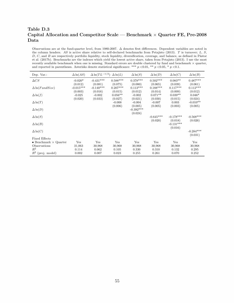
Table D.3Capital Allocation and Competitor Scale — Benchmark × Quarter FE, Pre-2008Data

Observations are at the fund-quarter level, from 1980-2007. ∆ denotes first differences. Dependent variables are noted inthe column headers. AS is active share relative to self-declared benchmarks from Petajisto (2013). T is turnover; L, S,D, C, and B are respectively portfolio liquidity, stock liquidity, diversification, coverage, and balance, as defined in Pástoret al. (2017b). Benchmarks are the indexes which yield the lowest active share, taken from Petajisto (2013). I use the mostrecently available benchmark when one is missing. Standard errors are double clustered by fund and benchmark × quarter,and reported in parentheses. Asterisks denote statistical significance: *** p <0.01, ** p <0.05, * p <0.1.


∆CS -0.020* -0.431*** 0.588*** 0.378*** 0.502*** 0.083** 0.487***(0.012) (0.081) (0.075) (0.080) (0.065) (0.039) (0.061)

∆ ln(FundSize) -0.015*** -0.140*** 0.207*** 0.113*** 0.188*** 0.117*** 0.112***(0.003) (0.016) (0.015) (0.012) (0.014) (0.009) (0.012)

∆ ln(f) -0.025 -0.002 0.056** -0.002 0.071** 0.039** 0.046*(0.020) (0.033) (0.027) (0.021) (0.030) (0.015) (0.024)

∆ ln(T ) -0.008 -0.004 -0.007 0.003 -0.010**(0.006) (0.005) (0.005) (0.003) (0.005)

∆ ln(D) -0.392***(0.024)

∆ ln(S) -0.645*** -0.178*** -0.568***(0.020) (0.018) (0.026)

∆ ln(B) -0.131***(0.016)

∆ ln(C) -0.284***(0.031)

Fixed Effects• Benchmark × Quarter Yes Yes Yes Yes Yes Yes YesObservations 31,063 30,968 30,968 30,968 30,968 30,968 30,968R2 0.114 0.062 0.105 0.330 0.310 0.132 0.295R2 (proj. model) 0.002 0.007 0.023 0.255 0.261 0.070 0.252

55

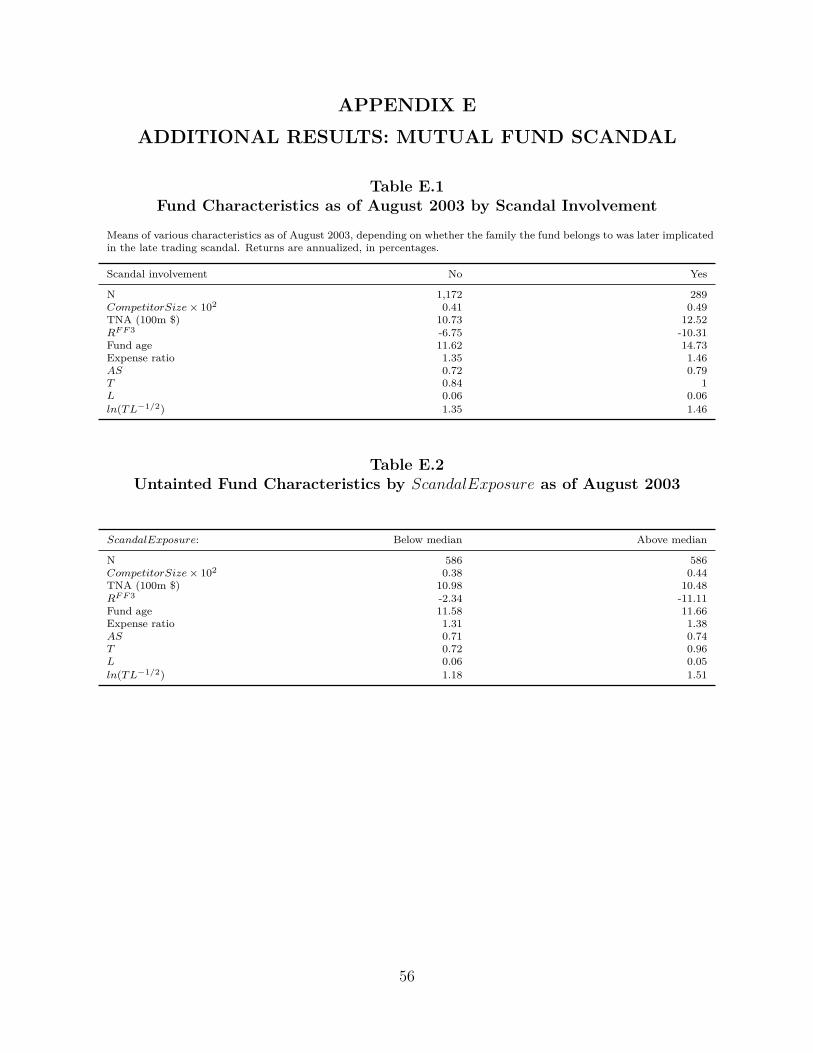
APPENDIX EADDITIONAL RESULTS: MUTUAL FUND SCANDAL

Table E.1Fund Characteristics as of August 2003 by Scandal Involvement

Means of various characteristics as of August 2003, depending on whether the family the fund belongs to was later implicatedin the late trading scandal. Returns are annualized, in percentages.

Scandal involvement No Yes

N 1,172 289CompetitorSize× 102 0.41 0.49TNA (100m $) 10.73 12.52RF F 3 -6.75 -10.31Fund age 11.62 14.73Expense ratio 1.35 1.46AS 0.72 0.79T 0.84 1L 0.06 0.06ln(TL−1/2) 1.35 1.46

Table E.2Untainted Fund Characteristics by ScandalExposure as of August 2003

ScandalExposure: Below median Above median

N 586 586CompetitorSize× 102 0.38 0.44TNA (100m $) 10.98 10.48RF F 3 -2.34 -11.11Fund age 11.58 11.66Expense ratio 1.31 1.38AS 0.71 0.74T 0.72 0.96L 0.06 0.05ln(TL−1/2) 1.18 1.51

56

Table E.3Capital Allocation and ScandalExposure: Testing for Pre-Trends

Dependent variables are identified in the column headers. ln(C.S.) is an abbreviation for ln(CompetitorSize). Observationsare at the fund-report date level, including only funds not directly involved in the scandal over the period [2003m8 −W, 2003m8], where W corresponds to the number of years specified in the panel headers. t × ScanEx is the interaction ofa linear time trend with ScandalExposure (normalized by its interquartile range). Standard errors are double clustered byfund and portfolio group × time, and reported in parentheses. Asterisks denote statistical significance: *** p <0.01, **p <0.05, * p <0.1.



t× ScanEx 0.114 0.015 0.930 0.301 0.395 0.090 0.236 -0.107(0.429) (0.094) (0.584) (0.453) (0.388) (0.397) (0.223) (0.332)

ln(FundSize) 0.083 0.026 -0.068 0.090 0.052 0.075 0.023 0.063(0.060) (0.025) (0.069) (0.066) (0.051) (0.064) (0.037) (0.051)

ln(f) 0.078 0.065 0.307 0.042 0.012 0.045 -0.058 0.101(0.182) (0.063) (0.187) (0.180) (0.097) (0.176) (0.109) (0.130)

ln(T ) -0.008 -0.000 -0.009 -0.011 -0.001(0.020) (0.015) (0.019) (0.015) (0.015)

ln(D) -0.350***(0.075)

ln(S) -0.527*** -0.273*** -0.346***(0.129) (0.083) (0.117)

ln(B) -0.126**(0.056)

ln(C) -0.235**(0.103)



t× ScanEx 0.270 -0.010 0.563* 0.146 -0.005 0.179 -0.018 0.213(0.208) (0.055) (0.325) (0.239) (0.145) (0.241) (0.134) (0.208)

ln(FundSize) 0.196*** -0.012 -0.197*** 0.262*** 0.142*** 0.221*** 0.088*** 0.162***(0.032) (0.009) (0.043) (0.041) (0.031) (0.038) (0.021) (0.034)

ln(f) -0.023 -0.021 0.278*** 0.014 -0.078 0.068 0.018 0.058(0.080) (0.034) (0.103) (0.107) (0.081) (0.091) (0.062) (0.082)

ln(T ) -0.016 -0.017 -0.008 -0.009 -0.001(0.026) (0.017) (0.023) (0.015) (0.017)

ln(D) -0.304***(0.037)

ln(S) -0.538*** -0.241*** -0.369***(0.078) (0.054) (0.076)

ln(B) -0.106***(0.036)

ln(C) -0.179***(0.063)


57

Table E.4Capital Allocation and the Scandal: Before and After Analysis — Benchmark ×Time FE

Dependent variables are identified in the column headers. ln(C.S.) is an abbreviation for ln(CompetitorSize). Observations are at the fund-report date level, including only funds not directly involved in the scandal over the period {(2003m8 − W, 2003m8], [2004m11, 2004m11 + W )},where W corresponds to the number of years specified in the panel headers. I × ScanEx is the interaction of ScandalExposure (normalizedby its interquartile range) and an indicator for the post-scandal period. Benchmarks are the indexes which yield the lowest active share, takenfrom Petajisto (2013). I use the most recently available benchmark when one is missing. Standard errors are double clustered by fund andbenchmark × date, and reported in parentheses. Asterisks denote statistical significance: *** p <0.01, ** p <0.05, * p <0.1.

Dep. Var.: ln(C.S.) ln(AS) ln(T L−1/2) ln(L) ln(S) ln(D) ln(C) ln(B)


I × ScanEx -0.065*** 0.018*** -0.015 -0.097*** -0.068*** -0.062** -0.035** -0.030(0.022) (0.006) (0.038) (0.029) (0.023) (0.025) (0.016) (0.020)

ln(F undSize) 0.125*** -0.006 -0.120*** 0.145*** 0.054*** 0.126*** 0.056*** 0.077***(0.021) (0.006) (0.032) (0.026) (0.014) (0.026) (0.019) (0.017)

ln(f) 0.024 -0.015 0.082 0.036 -0.060 0.083 0.068 0.020(0.106) (0.027) (0.149) (0.119) (0.074) (0.114) (0.072) (0.085)

ln(T ) -0.060** -0.055*** -0.029 0.024 -0.054***(0.028) (0.016) (0.027) (0.015) (0.020)

ln(D) -0.189***(0.024)

ln(S) -0.429*** -0.255*** -0.198***(0.055) (0.045) (0.051)

ln(B) -0.045(0.033)

ln(C) -0.067(0.048)

Fixed Effects• Fund Yes Yes Yes Yes Yes Yes Yes Yes• Benchmark × Time Yes Yes Yes Yes Yes Yes Yes YesObservations 6,549 6,067 6,464 6,464 6,464 6,464 6,464 6,464R2 0.931 0.932 0.905 0.966 0.990 0.944 0.948 0.899R2 (proj. model) 0.043 0.008 0.012 0.052 0.108 0.101 0.081 0.046


I × ScanEx -0.032 0.020*** -0.014 -0.085*** -0.080*** -0.038 -0.036** -0.004(0.023) (0.006) (0.038) (0.030) (0.024) (0.026) (0.017) (0.020)

ln(F undSize) 0.140*** -0.010* -0.169*** 0.166*** 0.059*** 0.144*** 0.063*** 0.088***(0.018) (0.006) (0.026) (0.024) (0.013) (0.023) (0.016) (0.017)

ln(f) -0.075 0.007 0.181 -0.076 -0.144** 0.018 0.050 -0.030(0.071) (0.025) (0.129) (0.109) (0.063) (0.094) (0.063) (0.074)

ln(T ) -0.045* -0.047*** -0.017 0.024* -0.041***(0.023) (0.012) (0.022) (0.013) (0.015)

ln(D) -0.171***(0.020)

ln(S) -0.404*** -0.238*** -0.187***(0.044) (0.036) (0.044)

ln(B) -0.042*(0.025)

ln(C) -0.060*(0.036)


58

Table E.5Capital Allocation and ScandalExposure: Testing for Pre-Trends — Benchmark× Time FE

Dependent variables are identified in the column headers. ln(C.S.) is an abbreviation for ln(CompetitorSize). Observations are at the fund-report date level, including only funds not directly involved in the scandal over the period [2003m8 − W, 2003m8], where W corresponds tothe number of years specified in the panel headers. t × ScanEx is the interaction a linear time trend with ScandalExposure (normalized byits interquartile range). Benchmarks are the indexes which yield the lowest active share, taken from Petajisto (2013). I use the most recentlyavailable benchmark when one is missing. Standard errors are double clustered by fund and benchmark × time, and reported in parentheses.Asterisks denote statistical significance: *** p <0.01, ** p <0.05, * p <0.1.



t × ScanEx 0.178 0.067 1.072 0.093 -0.270 0.262 -0.069 0.353(0.466) (0.112) (0.881) (0.469) (0.353) (0.436) (0.245) (0.405)

ln(F undSize) 0.076 0.015 -0.059 0.079 0.042 0.068 0.004 0.072*(0.056) (0.016) (0.076) (0.055) (0.030) (0.055) (0.036) (0.041)

ln(f) 0.157 0.037 0.297 0.152 0.082 0.131 -0.010 0.154(0.204) (0.047) (0.264) (0.161) (0.090) (0.154) (0.078) (0.136)

ln(T ) -0.013 -0.003 -0.013 -0.013 -0.003(0.023) (0.016) (0.022) (0.016) (0.017)

ln(D) -0.294***(0.056)

ln(S) -0.598*** -0.321*** -0.379***(0.077) (0.085) (0.103)

ln(B) -0.124*(0.072)

ln(C) -0.220*(0.132)



t × ScanEx 0.386 -0.012 0.850* 0.311 -0.050 0.400 -0.041 0.474*(0.294) (0.052) (0.439) (0.308) (0.183) (0.292) (0.139) (0.267)

ln(F undSize) 0.199*** -0.015 -0.199*** 0.283*** 0.139*** 0.241*** 0.095*** 0.176***(0.037) (0.010) (0.048) (0.045) (0.026) (0.044) (0.024) (0.041)

ln(f) -0.015 -0.025 0.322*** 0.019 -0.072 0.071 0.031 0.049(0.083) (0.031) (0.106) (0.107) (0.072) (0.094) (0.059) (0.082)

ln(T ) -0.008 -0.013 -0.001 -0.003 0.002(0.025) (0.016) (0.023) (0.015) (0.018)

ln(D) -0.267***(0.037)

ln(S) -0.513*** -0.248*** -0.332***(0.084) (0.058) (0.077)

ln(B) -0.101**(0.040)

ln(C) -0.173**(0.072)


59

Table E.6Capital Allocation and ScandalOutF low: Testing for Pre-Trends

Dependent variables are identified in the column headers. ln(C.S.) is an abbreviation for ln(CompetitorSize). Observations are at thefund-report date level, including only funds not directly involved in the scandal over the period [2003m8 − W, 2003m8], where W denotes thenumber of years specified. ScandalOutF low is the fund-level mean ScandalOutF low over the specified post-scandal window, normalized byinterquartile range. Benchmarks are the indexes which yield the lowest active share, taken from Petajisto (2013). I use the most recentlyavailable benchmark when one is missing. Standard errors are double clustered by fund and portfolio group × time, and reported in parentheses.Asterisks denote statistical significance: *** p <0.01, ** p <0.05, * p <0.1.



t × ScandalOutF low 0.049* -0.002 0.046 0.030 0.030 0.017 -0.008 0.026(0.027) (0.007) (0.040) (0.027) (0.023) (0.024) (0.015) (0.019)

ln(F undSize) 0.075 0.024 -0.067 0.067 0.052 0.048 0.005 0.049(0.056) (0.023) (0.064) (0.061) (0.054) (0.058) (0.035) (0.046)

ln(f) 0.067 0.057 0.295 0.041 0.026 0.033 -0.057 0.087(0.176) (0.060) (0.182) (0.174) (0.096) (0.172) (0.103) (0.129)

ln(T ) -0.003 0.002 -0.005 -0.006 -0.001(0.019) (0.013) (0.019) (0.014) (0.014)

ln(D) -0.366***(0.074)

ln(S) -0.561*** -0.274*** -0.376***(0.134) (0.081) (0.123)

ln(B) -0.115**(0.053)

ln(C) -0.221**(0.103)



t × ScandalOutF low 0.024 -0.006 0.036* 0.020 0.009 0.019 0.007 0.014(0.016) (0.006) (0.020) (0.017) (0.011) (0.016) (0.010) (0.012)

ln(F undSize) 0.184*** -0.009 -0.198*** 0.246*** 0.141*** 0.212*** 0.077*** 0.162***(0.033) (0.008) (0.043) (0.041) (0.031) (0.038) (0.020) (0.034)

ln(f) -0.027 -0.024 0.273*** 0.026 -0.047 0.060 0.012 0.055(0.081) (0.032) (0.103) (0.107) (0.084) (0.089) (0.058) (0.083)

ln(T ) -0.009 -0.018 -0.001 -0.009 0.008(0.025) (0.017) (0.023) (0.014) (0.017)

ln(D) -0.339***(0.041)

ln(S) -0.604*** -0.248*** -0.436***(0.080) (0.050) (0.082)

ln(B) -0.106***(0.033)

ln(C) -0.184***(0.061)


60

Table E.7Capital Allocation and ScandalOutF low — Benchmark × Time FE

Dependent variables are identified in the column headers. ln(C.S.) is an abbreviation for ln(CompetitorSize). Observations are at thefund-report date level, including only funds not directly involved in the scandal over the period {[2003m9 − W, 2004m10 + W ]}, where Wcorresponds to the number of years specified. ScandalOutF low is normalized by its interquartile range. Benchmarks are the indexes whichyield the lowest active share, taken from Petajisto (2013). I use the most recently available benchmark when one is missing. Standard errorsare double clustered by fund and benchmark × time, and reported in parentheses. Asterisks denote statistical significance: *** p <0.01, **p <0.05, * p <0.1.



ScandalOutF low -0.203*** 0.058*** 0.092** -0.250*** -0.111*** -0.215*** -0.074*** -0.163***(0.021) (0.008) (0.038) (0.030) (0.019) (0.028) (0.018) (0.020)

ln(F undSize) 0.096*** -0.005 -0.103*** 0.127*** 0.054*** 0.111*** 0.065*** 0.059***(0.017) (0.005) (0.028) (0.022) (0.012) (0.021) (0.016) (0.015)

ln(f) -0.050 -0.010 0.093 -0.011 -0.055 0.023 0.065 -0.036(0.076) (0.023) (0.116) (0.090) (0.055) (0.088) (0.058) (0.065)

ln(T ) -0.057*** -0.040*** -0.040** 0.010 -0.052***(0.019) (0.011) (0.019) (0.011) (0.015)

ln(D) -0.227***(0.022)

ln(S) -0.501*** -0.265*** -0.295***(0.049) (0.038) (0.049)

ln(B) -0.091***(0.029)

ln(C) -0.144***(0.044)



ScandalOutF low -0.161*** 0.059*** 0.097*** -0.226*** -0.106*** -0.188*** -0.070*** -0.134***(0.019) (0.007) (0.032) (0.027) (0.018) (0.026) (0.018) (0.018)

ln(F undSize) 0.118*** -0.008 -0.153*** 0.147*** 0.058*** 0.129*** 0.066*** 0.075***(0.015) (0.005) (0.023) (0.021) (0.012) (0.020) (0.015) (0.015)

ln(f) -0.113* 0.011 0.200* -0.110 -0.145** -0.030 0.044 -0.074(0.059) (0.022) (0.105) (0.097) (0.058) (0.084) (0.055) (0.068)

ln(T ) -0.044** -0.039*** -0.025 0.014 -0.040***(0.019) (0.010) (0.018) (0.011) (0.013)

ln(D) -0.209***(0.019)

ln(S) -0.481*** -0.258*** -0.269***(0.040) (0.033) (0.042)

ln(B) -0.076***(0.024)

ln(C) -0.113***(0.034)


61

Table E.8Capital Allocation and ScandalOutF low: Testing for Pre-Trends — Benchmark× Time FE

Dependent variables are identified in the column headers. ln(C.S.) is an abbreviation for ln(CompetitorSize). Observations are at thefund-report date level, including only funds not directly involved in the scandal over the period [2003m8 − W, 2003m8], where W denotes thenumber of years specified. ScandalOutF low is the fund-level mean ScandalOutF low over the specified post-scandal window, normalized byinterquartile range. Benchmarks are the Standard errors are double clustered by fund and benchmark × time, and reported in parentheses.Asterisks denote statistical significance: *** p <0.01, ** p <0.05, * p <0.1.



t × ScandalOutF low 0.076*** -0.000 0.092* 0.020 0.005 0.020 -0.005 0.027(0.027) (0.008) (0.053) (0.030) (0.018) (0.030) (0.019) (0.026)

ln(F undSize) 0.074 0.013 -0.061 0.064 0.051 0.047 -0.006 0.057(0.054) (0.015) (0.075) (0.051) (0.034) (0.051) (0.033) (0.039)

ln(f) 0.153 0.026 0.269 0.160 0.096 0.134 -0.007 0.153(0.200) (0.046) (0.238) (0.163) (0.092) (0.156) (0.077) (0.135)

ln(T ) -0.010 -0.003 -0.010 -0.010 -0.002(0.021) (0.015) (0.021) (0.015) (0.016)

ln(D) -0.302***(0.055)

ln(S) -0.623*** -0.317*** -0.403***(0.077) (0.082) (0.097)

ln(B) -0.113*(0.068)

ln(C) -0.208(0.130)



t × ScandalOutF low 0.056*** -0.008 0.037 0.037* 0.021* 0.031 0.008 0.027(0.018) (0.007) (0.023) (0.021) (0.011) (0.021) (0.012) (0.017)

ln(F undSize) 0.186*** -0.011 -0.202*** 0.260*** 0.132*** 0.227*** 0.083*** 0.173***(0.037) (0.009) (0.050) (0.043) (0.026) (0.041) (0.022) (0.039)

ln(f) -0.030 -0.027 0.326*** 0.015 -0.054 0.050 0.022 0.034(0.081) (0.029) (0.108) (0.105) (0.073) (0.091) (0.056) (0.080)

ln(T ) -0.002 -0.016 0.007 -0.004 0.011(0.024) (0.016) (0.023) (0.014) (0.019)

ln(D) -0.298***(0.040)

ln(S) -0.584*** -0.258*** -0.402***(0.086) (0.056) (0.085)

ln(B) -0.101***(0.039)

ln(C) -0.176**(0.070)


62

Table E.9Capital Allocation and the Scandal: Instrumenting Competitor Size with Ab-normal FlowsDependent variables are identified in the column headers. ln(C.S.) is an abbreviation for ln(CompetitorSize). Observationsare at the fund-report date level, including only funds not directly involved in the scandal over the period {[2003m9 −W, 2004m10 + W ]}, where W corresponds to the number of years specified. ScandalOutF low is the similarity-weightedcumulative abnormal outflows attributable to the scandal among involved funds. ScandalOutF low is normalized by itsinterquartile range. Regressions are estimated via two stage least squares, instrumenting for ln(CompetitorSizei,t) withScandalOutF lowi,t. The F-statistic of the first stage relation is reported at the bottom of each panel. Standard errorsare double clustered by fund and portfolio group × time, and are reported in parentheses. Asterisks denote statisticalsignificance: *** p <0.01, ** p <0.05, * p <0.1.

Dep. Var.: ln(AS) ln(TL−1/2) ln(L) ln(S) ln(D) ln(C) ln(B)


ln(CompetitorSize) -0.330*** -0.668*** 1.213*** 1.015*** 1.078*** 0.826*** 0.856***(0.046) (0.141) (0.090) (0.115) (0.089) (0.141) (0.074)

ln(FundSize) 0.021** -0.068** 0.030* 0.026* 0.025 0.030* 0.004(0.009) (0.031) (0.018) (0.015) (0.017) (0.017) (0.012)

ln(f) -0.025 0.034 0.034 0.012 0.049 0.067 -0.009(0.032) (0.106) (0.080) (0.069) (0.074) (0.066) (0.051)

ln(T ) -0.043*** -0.041*** -0.032*** -0.014 -0.043***(0.012) (0.011) (0.011) (0.010) (0.009)

ln(D) -0.739***(0.058)

ln(S) -0.705*** -0.560*** -0.528***(0.035) (0.060) (0.040)

ln(B) -0.637***(0.097)

ln(C) -0.422***(0.041)

Fixed Effects• Fund Yes Yes Yes Yes Yes Yes Yes• Time Yes Yes Yes Yes Yes Yes YesObservations 10,324 11,689 11,689 11,689 11,689 11,689 11,689F (first stage) 107.7 111.7 111.4 70.9 100.2 44.6 90.9



ln(FundSize) 0.028*** -0.097*** 0.018 0.013 0.020 0.020 0.007(0.009) (0.027) (0.019) (0.016) (0.017) (0.017) (0.012)

ln(f) -0.034 0.102 0.034 -0.001 0.076 0.094* 0.004(0.026) (0.097) (0.067) (0.064) (0.058) (0.052) (0.048)

ln(T ) -0.035*** -0.037*** -0.020* -0.003 -0.033***(0.013) (0.011) (0.012) (0.011) (0.009)

ln(D) -0.775***(0.061)

ln(S) -0.657*** -0.513*** -0.484***(0.029) (0.049) (0.037)

ln(B) -0.607***(0.088)

ln(C) -0.408***(0.038)


63

Table E.10Capital Allocation and the Scandal: Instrumenting Competitor Size with Ab-normal Flows — Benchmark × Time FEDependent variables are identified in the column headers. ln(C.S.) is an abbreviation for ln(CompetitorSize). Ob-servations are at the fund-report date level, including only funds not directly involved in the scandal over the period{[2003m9 −W, 2004m10 +W ]}, where W corresponds to the number of years specified. ScandalOutF low is the similarity-weighted cumulative abnormal outflows attributable to the scandal among involved funds. ScandalOutF low is normalizedby its interquartile range. I estimate regressions via two stage least squares, instrumenting for ln(CompetitorSizei,t) withScandalOutF lowi,t. The F-statistic of the first stage relation is reported at the bottom of each panel. Standard errors aredouble clustered by fund and benchmark × time, and are reported in parentheses. Asterisks denote statistical significance:*** p <0.01, ** p <0.05, * p <0.1.

Dep. Var.: ln(AS) ln(TL−1/2) ln(L) ln(S) ln(D) ln(C) ln(B)


ln(CompetitorSize) -0.297*** -0.453** 1.225*** 0.961*** 1.125*** 0.839*** 0.955***(0.045) (0.177) (0.107) (0.154) (0.108) (0.200) (0.094)

ln(FundSize) 0.021** -0.059* 0.008 0.005 0.008 0.016 -0.009(0.008) (0.033) (0.020) (0.015) (0.019) (0.019) (0.014)

ln(f) -0.022 0.077 0.030 0.004 0.047 0.057 0.006(0.030) (0.110) (0.079) (0.065) (0.075) (0.066) (0.055)

ln(T ) -0.041*** -0.037*** -0.032*** -0.014 -0.041***(0.012) (0.010) (0.011) (0.011) (0.009)

ln(D) -0.700***(0.081)

ln(S) -0.706*** -0.562*** -0.545***(0.040) (0.080) (0.044)

ln(B) -0.646***(0.139)

ln(C) -0.463***(0.047)




ln(FundSize) 0.033*** -0.084*** -0.016 -0.016 -0.010 -0.005 -0.018(0.010) (0.031) (0.023) (0.020) (0.021) (0.024) (0.016)

ln(f) -0.031 0.143 0.024 0.002 0.059 0.063 0.019(0.025) (0.100) (0.068) (0.067) (0.059) (0.054) (0.049)

ln(T ) -0.035*** -0.035*** -0.024** -0.016 -0.033***(0.013) (0.012) (0.012) (0.013) (0.009)

ln(D) -0.834***(0.116)

ln(S) -0.689*** -0.611*** -0.536***(0.037) (0.094) (0.044)

ln(B) -0.795***(0.184)

ln(C) -0.499***(0.050)


64

Table E.11Investor Flows and the Scandal

The dependent variable is net flows in monthly percent units. Observations are at the fund-month level, including onlyfunds untainted by the scandal, over 1-2 year windows around the scandal. I is an indicator for the post scandal period.ScandalExposure (ScanEx) and ScandalOutF low are normalized by interquartile range. Benchmarks are the indexes whichyield the lowest active share, taken from Petajisto (2013). Standard errors are double clustered by fund and portfolio group× month in the month FE specifications, and by fund and benchmark × month in the benchmark × month specifications,reported in parentheses. Asterisks denote statistical significance: *** p <0.01, ** p <0.05, * p <0.1.

(1) (2) (3) (4) (5) (6) (7) (8)

1 year window 2 year window

Panel A: Ignoring Past Performance

I × ScanEx -0.102 -0.052 0.286* 0.218(0.161) (0.194) (0.152) (0.167)

ScandalOutF low 0.082 0.068 0.369*** 0.278**(0.136) (0.166) (0.111) (0.124)

Fixed Effects• Fund Yes Yes Yes Yes Yes Yes Yes Yes• Month Yes No Yes No Yes No Yes No• Benchmark × Month No Yes No Yes No Yes No YesObservations 25,179 23,122 41,715 38,293 48,883 44,916 66,252 60,849R2 0.296 0.307 0.297 0.307 0.234 0.257 0.243 0.261R2 (proj. model) 0.000 0.000 0.000 0.000 0.001 0.000 0.001 0.001

Panel B: Controlling for Past Performance

I × ScanEx -0.343** -0.140 -0.248* -0.080(0.148) (0.179) (0.128) (0.149)

ScandalOutF low -0.103 -0.242 0.102 -0.007(0.125) (0.155) (0.093) (0.109)

RF F 3t−1 0.181*** 0.188*** 0.176*** 0.192*** 0.168*** 0.165*** 0.165*** 0.169***

(0.025) (0.027) (0.022) (0.022) (0.021) (0.019) (0.018) (0.017)RF F 3

t−2 0.158*** 0.176*** 0.159*** 0.172*** 0.161*** 0.166*** 0.159*** 0.164***(0.021) (0.022) (0.019) (0.018) (0.020) (0.017) (0.017) (0.015)

RF F 3t−3 0.151*** 0.158*** 0.137*** 0.148*** 0.140*** 0.145*** 0.133*** 0.141***

(0.024) (0.021) (0.020) (0.017) (0.020) (0.015) (0.017) (0.014)RF F 3

t−4 0.080*** 0.087*** 0.079*** 0.085*** 0.099*** 0.103*** 0.094*** 0.099***(0.018) (0.018) (0.015) (0.015) (0.017) (0.017) (0.015) (0.014)

RF F 3t−5 0.085*** 0.098*** 0.082*** 0.091*** 0.099*** 0.109*** 0.093*** 0.102***

(0.024) (0.022) (0.018) (0.016) (0.019) (0.016) (0.016) (0.014)RF F 3

t−6 0.102*** 0.118*** 0.086*** 0.101*** 0.116*** 0.126*** 0.102*** 0.114***(0.019) (0.021) (0.015) (0.017) (0.016) (0.016) (0.013) (0.014)

RF F 3t−7 0.069*** 0.080*** 0.058*** 0.063*** 0.104*** 0.110*** 0.088*** 0.092***

(0.026) (0.021) (0.019) (0.017) (0.019) (0.018) (0.016) (0.016)RF F 3

t−8 0.093*** 0.104*** 0.066*** 0.075*** 0.094*** 0.094*** 0.076*** 0.078***(0.025) (0.018) (0.019) (0.015) (0.017) (0.014) (0.014) (0.012)

RF F 3t−9 0.087*** 0.098*** 0.065*** 0.081*** 0.105*** 0.114*** 0.086*** 0.101***

(0.023) (0.017) (0.017) (0.014) (0.017) (0.014) (0.014) (0.011)RF F 3

t−10 0.120*** 0.135*** 0.077*** 0.085*** 0.103*** 0.115*** 0.079*** 0.089***(0.023) (0.021) (0.016) (0.015) (0.015) (0.016) (0.013) (0.013)

RF F 3t−11 0.120*** 0.130*** 0.065*** 0.080*** 0.106*** 0.108*** 0.074*** 0.083***

(0.019) (0.019) (0.015) (0.014) (0.013) (0.013) (0.012) (0.011)RF F 3

t−12 0.067*** 0.090*** 0.052*** 0.074*** 0.066*** 0.075*** 0.056*** 0.070***(0.019) (0.018) (0.015) (0.014) (0.013) (0.011) (0.012) (0.010)

Fixed Effects• Fund Yes Yes Yes Yes Yes Yes Yes Yes• Month Yes No Yes No Yes No Yes No• Benchmark × Month No Yes No Yes No Yes No YesObservations 24,529 22,672 40,718 37,595 47,247 43,770 64,241 59,440R2 0.314 0.329 0.311 0.326 0.257 0.280 0.260 0.280R2 (proj. model) 0.025 0.028 0.019 0.022 0.035 0.035 0.028 0.028

65

APPENDIX FDATA CONSTRUCTION

Code for reproducing the paper in full is available at https://github.com/laszlo-jakab/competitor-scale.1 For a standalone toolbox to calculate the CompetitorSize variable us-ing portfolio weights and fund sizes, see the R package compsizer, available at https://github.com/laszlo-jakab/compsizer.

F.1 CRSP Survivor-Bias-Free US Mutual Fund Database

F.1.1 Source Datasets

I download the following datasets from WRDS: MONTHLY_TNA, MONTHLY_RETURNS,MONTHLY_NAV, FUND_HDR, FUND_HDR_HIST, FUND_FEES, FUND_STYLE. The following is asummary of the steps I took for cleaning the data.

F.1.2 Data Cleaning

• MONTHLY_TNA

– Set mtna = -99 to missing.– Keep observations with positive, non-missing mtna.– Align caldt across share classes each month by taking the min (in a few cases,

caldt is beyond the last trading day).

• MONTHLY_RETURNS

– keep observations with non-missing mret.– align caldt across share classes each month as above.– keep returns only if they apply for a single month, as evidenced by non-missing

mnav or mret in the previous month.

• FUND_FEES

– Set -99 to missing for all variables.– Set exp_ratio <= 0 to missing.– Make sure begdt and enddt do not overlap (in a handful of cases, the next begdt

is the same as the current enddt; if so, I decrement enndt by one day).– Break out turn_ratio, as begdt and enddt are not appropriate for this variable.– turn_ratio is valid for 12 months ending on fiscal_yearend when it is present,

otherwise, for the 12 months ending on begdt; construct custom beginning andend dates for turn_ratio based on this fact.

1. Programs built under R 3.4.3, using packages data.table 1.10.4-3, and zoo 1.8-1. Fixed effectsand instrumental variable regressions estimated using the lfe 2.6-2291 package (Gaure, 2013).

66

https://github.com/laszlo-jakab/competitor-scale

https://github.com/laszlo-jakab/competitor-scale

https://github.com/laszlo-jakab/compsizer

https://github.com/laszlo-jakab/compsizer

• FUND_HDR, FUND_HDR_HIST

– Append datasets.– Clean beginning and end dates.

F.1.3 Generating Fund-Level Dataset

1. Combine returns, TNA, expense ratio, turnover

• Match returns and TNA on crsp_fundno and caldt.• Overlap match combined returns and TNA to exp_ratio on crsp_fundno, and

begdt <= caldt <= enddt.• Perform similar overlap match for turnover, on user-defined beginning and end

dates.

2. Fill in gaps in mtna by carrying forward the last non-missing observation, compoundedby net returns.

3. Generate one-month lag TNA to be used as weights in the fund-level aggregation; fillin first observation for each fund by current TNA to retain as many observations aspossible (this is used only for the fund-level aggregation). Keep only if lagged TNA ispositive and non-missing.

4. Merge in the fund identifier wficn from MFLINKS.5. Generate gross returns as mret.gross = mret + exp_ratio / 12.6. Aggregate to fund level.

• For each of net returns, gross returns, expense ratio, and turnover, calculatelagged-TNA-weighted means at the fund-month level, using only non-missingobservations for each.

• Sum TNA by fund-month.• Merge fund-month level variables into single dataset.

7. Clean fund-month level dataset.

• Keep only if lagged TNA in 2017 dollars is in excess of 15 million.• If lagged TNA missing, drop if current TNA is below 15 million in 2017 dollars.• Drop if current TNA is zero.• Drop if expense ratio is below 0.1%.• Keep only if a fund has twelve months of available observations.

F.2 CRSP US Stock Database

I download the following datasets from WRDS: MSF, STOCKNAMES. The following is a summaryof the steps I took for cleaning the data. - Set prc = -99 to missing, and replace the variablewith its absolute value. - Keep if prc and shrout are non-missing. - Overlap match toSTOCKNAMES on crsp_fundno and namedt <= caldt <= nameendt|. - Keep only commonstock (shrcd 10 or 11).

67

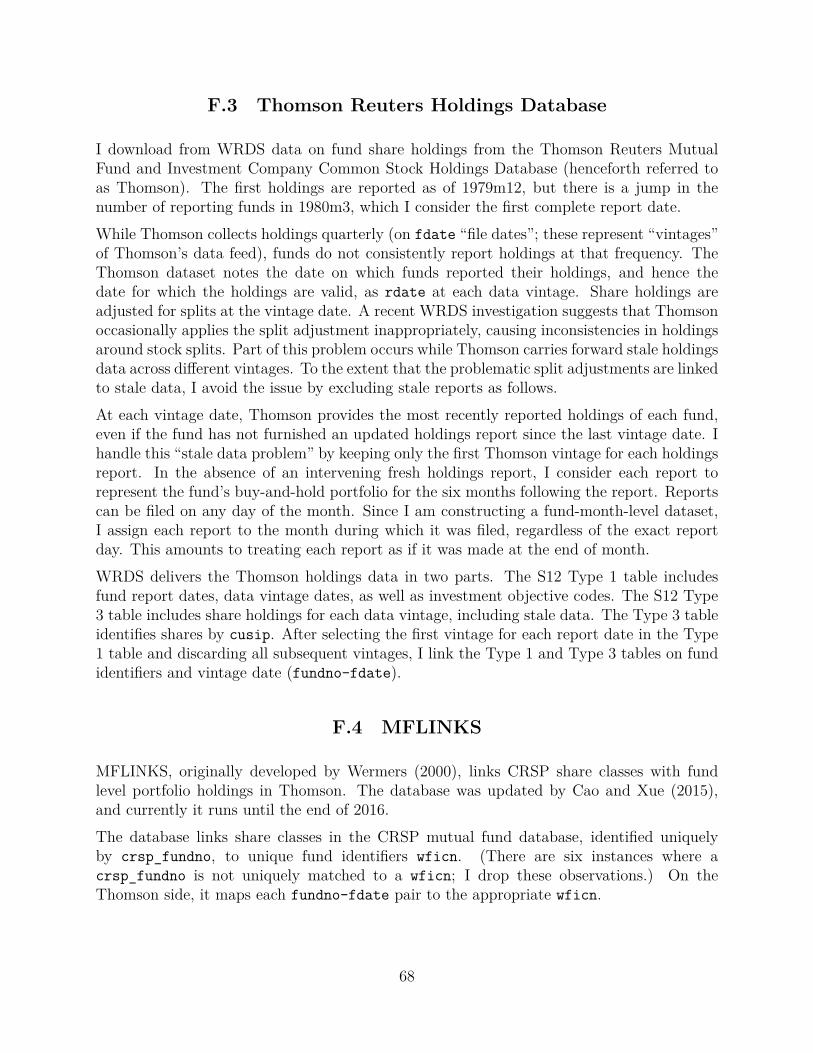
F.3 Thomson Reuters Holdings Database

I download from WRDS data on fund share holdings from the Thomson Reuters MutualFund and Investment Company Common Stock Holdings Database (henceforth referred toas Thomson). The first holdings are reported as of 1979m12, but there is a jump in thenumber of reporting funds in 1980m3, which I consider the first complete report date.While Thomson collects holdings quarterly (on fdate “file dates”; these represent “vintages”of Thomson’s data feed), funds do not consistently report holdings at that frequency. TheThomson dataset notes the date on which funds reported their holdings, and hence thedate for which the holdings are valid, as rdate at each data vintage. Share holdings areadjusted for splits at the vintage date. A recent WRDS investigation suggests that Thomsonoccasionally applies the split adjustment inappropriately, causing inconsistencies in holdingsaround stock splits. Part of this problem occurs while Thomson carries forward stale holdingsdata across different vintages. To the extent that the problematic split adjustments are linkedto stale data, I avoid the issue by excluding stale reports as follows.At each vintage date, Thomson provides the most recently reported holdings of each fund,even if the fund has not furnished an updated holdings report since the last vintage date. Ihandle this “stale data problem” by keeping only the first Thomson vintage for each holdingsreport. In the absence of an intervening fresh holdings report, I consider each report torepresent the fund’s buy-and-hold portfolio for the six months following the report. Reportscan be filed on any day of the month. Since I am constructing a fund-month-level dataset,I assign each report to the month during which it was filed, regardless of the exact reportday. This amounts to treating each report as if it was made at the end of month.WRDS delivers the Thomson holdings data in two parts. The S12 Type 1 table includesfund report dates, data vintage dates, as well as investment objective codes. The S12 Type3 table includes share holdings for each data vintage, including stale data. The Type 3 tableidentifies shares by cusip. After selecting the first vintage for each report date in the Type1 table and discarding all subsequent vintages, I link the Type 1 and Type 3 tables on fundidentifiers and vintage date (fundno-fdate).

F.4 MFLINKS

MFLINKS, originally developed by Wermers (2000), links CRSP share classes with fundlevel portfolio holdings in Thomson. The database was updated by Cao and Xue (2015),and currently it runs until the end of 2016.The database links share classes in the CRSP mutual fund database, identified uniquelyby crsp_fundno, to unique fund identifiers wficn. (There are six instances where acrsp_fundno is not uniquely matched to a wficn; I drop these observations.) On theThomson side, it maps each fundno-fdate pair to the appropriate wficn.

68

F.5 Calculating Fund Portfolio Weights

F.5.1 Linking CUSIP and permno

I use the STOCKNAMES file to produce a linking table between CUSIP and permno in orderto combine share Thomson share holding data with CRSP stock data. I take ncusip as therelevant identifier in this file; when it is missing, I fill it in with the appropriate cusip. Ithen generate all unique pairs between the (filled-in) ncusip and permno. This algorithmproduces a one to many mapping between (filled-in) ncusip and permno.

F.5.2 Applying share adjustment

Holdings in Thomson are adjusted for splits as of the vintage date. I therefore matchholdings to CRSP cumulative share adjustment factors (cfacshr) by vintage date asshares=shares*cfacshr. I retain only share holdings which can be matched to records inCRSP classified as US common equity.

F.5.3 Prices

After adjusting shares, I forward fill portfolio holdings for up to 6 months between reportdates, simulating a buy-and-hold strategy. I then match holdings with prices and cumulativeprice adjustment factors (cfacpr) on the (forward-filled) report dates, and calculate holdingvalues as shares*prc/cfacpr at each date, and use these to calculate portfolio weights.

F.6 Identifying actively managed domestic equity funds

The following steps describe the algorithm for identifying actively managed US equity funds.

1. Exclude funds without a wficn fund identifier from MFLINKS.2. Exclude funds that do not meet the data availability, size, or expense ratio requirements

in the CRSP mutual fund dataset.3. Exclude funds with investment objective codes (ioc) in the Thomson Reuters S12

Type 1 database of the following type:

• ioc = 1 International• ioc = 5 Municipal Bond• ioc = 6 Bond & Preferred• ioc = 7 Balanced• ioc = 8 Metals Remaining funds either have a missing investment objective

code, or are categorized as ioc = 2 Aggressive Growth, ioc==3 Growth, ioc= 4 Growth & Income, ioc = 9 Unclassified.

69

4. Drop if any share class of the fund is ever classified as an index fund by CRSP(index_fund_flag != ""), or if the name of any of the fund’s share classes evercontains “index” in the CRSP database.

5. Exclude if any of the fund’s share classes is ever assigned any of the following policycode (policy) in CRSP:

• Bal Balanced fund• B & P Bonds and preferred stock (mainly convertible funds)• Bonds Bonds• C & I Canadian and international• Hedge Leverage and/or short selling• Leases Holds equity in lease contracts• GS Government securities• MM Money market• Pfd Preferred stock• Spec Sector or highly speculative fund• TF Tax free fund• TFE Tax-free exchange fund• TFM Tax free money market fund

6. Use CRSP objective codes (crsp_obj_cd) to exclude target date funds and sectorfunds, as follows.

• Target date funds: exclude fund if any share class ever has crsp_obj_cd equalto MT

• Sector funds: exclude fund if any share class is ever has crsp_obj_cd beginningwith EDS

7. Exclude funds with any share class whose lower case name ever includes any of thefollowing geographical and allocation-related strings

• internat• euro• japan• emerging market• balanced• bond fund

8. To further ensure the exclusion of target date funds, drop funds with any share classeswhose lower case name ever includes any of the following strings

• 20[0-9][0-9]• retire• target

9. Exclude Tax-managed funds with any share classes whose lower case name ever includestax- or tax, followed by any of manage, efficien, exempt, smart, advantage, aware,or sensitive.

70

10. After the above filters are applied, I define domestic equity funds constructivelythrough the following procedure. Consider a share class domestic equity if

i. Lipper class indicates domestic equity. I consider this to be the case iflipper_class is any of

• EIEI Equity income• G Growth• LCCE Large cap core• LCGE Large cap growth• LCVE Large cap value• MCCE Mid cap core• MCGE Mid cap growth• MCVE Mid cap value• MLCE Multi cap core• MLGE Multi cap growth• MLVE Multi cap value• SCCE Small cap core• SCGE Small cap growth• SCVE Small cap value

ii. If Lipper class is unavailable, rely on Strategic Insights Objective Codes to identifyequity funds. I flag funds as domestic equity if si_obj_cd is any of

• AGG Equity US aggressive growth• GMC Equity US midcaps• GRI Equity US growth & income• GRO Equity US growth• ING Equity US income & growth

• SCG Equity US small companiesiii. If neither Lipper class nor Strategic Insights Objective Code is available, I use

Wiesenberger Fund Type codes. I flag funds as domestic equity if wbrger_obj_cdis any of - G Growth - G-I Growth-income - GCI Growth and current income -LTG Long term growth - MCG Maximum capital gains - SCG Small cap growth

I include a fund if any of its share classes is flagged as domestic equity by the above procedureat some point.

11. Drop if any share classes ever classified as fixed income, i.e. with crsp_obj_cd begin-ning with I

12. Drop funds if it is classified as a foreign fund (crsp_obj_cd beginning with EF) over25% of the time.

71

REFERENCES

Antón, M. and Polk, C. (2014). Connected stocks. Journal of Finance, 69(3):1099–1127.

Berk, J. B. and Green, R. C. (2004). Mutual fund flows and performance in rational markets.Journal of Political Economy, 112(6):1269–1295.

Berk, J. B. and van Binsbergen, J. H. (2015). Measuring skill in the mutual fund industry.Journal of Financial Economics, 118(1):1–20.

Berk, J. B., van Binsbergen, J. H., and Liu, B. (2017). Matching capital and labor. Journalof Finance, 72(6):2467–2504.

Blocher, J. (2016). Network externalities in mutual funds. Journal of Financial Markets,30:1–26.

Busse, J. A., Chordia, T., Jiang, L., and Tang, Y. (2017). Mutual fund trading costs.Working paper. Available at SSRN: https://ssrn.com/abstract=2350583.

Cao, B. and Xue, J. (2015). Mutual fund links update procedures. WRDS Re-search Note. Available at: https://wrds-web.wharton.upenn.edu/wrds/support/Data/_001Manuals%20and%20Overviews/_090MFLINKS/Mutual%20Fund%20Links%20Update%20Procedure.pdf.cfm.

Chamberlain, G. (1982). Multivariate regression models for panel data. Journal of Econo-metrics, 18(1):5–46.

Chen, J., Hong, H., Huang, M., and Kubik, J. D. (2004). Does fund size erode mutualfund performance? The role of liquidity and organization. American Economic Review,94(5):1276–1302.

Cohen, L. H., Malloy, C. J., and Nguyen, Q. H. (2016). Lazy prices. Working paper. Availableat SSRN: https://ssrn.com/abstract=1658471.

Cohen, R. B., Coval, J. D., and Pástor, Ľuboš. (2005). Judging fund managers by thecompany they keep. Journal of Finance, 60(3):1057–1096.

Coval, J. D. and Stafford, E. (2007). Asset fire sales (and purchases) in equity markets.Journal of Financial Economics, 86(2):479–512.

Cremers, M. (2017). Active share and the three pillars of active management: Skill, convic-tion and opportunity. Financial Analysts Journal, 73(2):61–79.

Cremers, M. and Petajisto, A. (2009). How active is your fund manager? A new measurethat predicts performance. Review of Financial Studies, 22(9):3329–3365.

Cremers, M., Petajisto, A., and Zitzewitz, E. W. (2012). Should benchmark indices havealpha? Revisiting performance evaluation. Critical Finance Review, 2:1–48.

Evans, R. (2000). Mutual fund incubation. Journal of Finance, 65(4):1581–1611.72

https://ssrn.com/abstract=2350583

https://wrds-web.wharton.upenn.edu/wrds/support/Data/_001Manuals%20and%20Overviews/_090MFLINKS/Mutual%20Fund%20Links%20Update%20Procedure.pdf.cfm




Fama, E. F. and French, K. R. (2010). Luck versus skill in the cross-section of mutual fundreturns. Journal of Finance, 65(5):1915–1947.

French, K. R. (2008). Presidential address: The cost of active investing. Journal of Finance,63(4):1537–1573.

Gaure, S. (2013). lfe: Linear group fixed effects. The R Journal, 5(2):104–117. Userdocumentation of the ’lfe’ package.

Gruber, M. J. (1996). Another puzzle: The growth in actively managed mutual funds.Journal of Finance, 51(3):783–810.

Harvey, C. R. and Liu, Y. (2017). Decreasing returns to scale, fund flows, and performance.Duke I&E Research Paper No. 2017-13. Available at SSRN: https://ssrn.com/abstract=2990737.

Hoberg, G., Kumar, N., and Prabhala, N. (2018). Mutual fund competition, managerialskill, and alpha persistence. Review of Financial Studies, 31(5):1896–1929.

Houge, T. and Wellman, J. (2005). Fallout from the mutual fund trading scandal. Journalof Business Ethics, 62:129–139.

Jensen, M. C. (1968). The performance of mutual funds in the period 1945–1964. Journalof Finance, 23(2):389–416.

Kacperczyk, M., Nieuwerburgh, S. V., and Veldkamp, L. (2016). A rational theory of mutualfunds’ attention allocation. Econometrica, 84(2):571–626.

Kacperczyk, M., Sialm, C., and Zheng, L. (2005). On the industry concentration of activelymanaged equity mutual funds. Journal of Finance, 60(4):1983–2011.

Kacperczyk, M., Sialm, C., and Zheng, L. (2008). Unobserved actions of mutual funds.Review of Financial Studies, 21(6):2379–2416.

Khan, M., Kogan, L., and Serafeim, G. (2012). Mutual fund trading pressure: Firm-levelstock price impact and timing of SEOs. Journal of Finance, 68(4):1371–1395.

Lou, D. (2012). A flow-based explanation for return predictability. Review of FinancialStudies, 25(12):3457–3489.

Malkiel, B. G. (1995). Returns from investing in equity mutual funds, 1971–1991. Journalof Finance, 50(2):549–572.

Malkiel, B. G. (2013). Asset management fees and the growth of finance. Journal of EconomicPerspectives, 27(2):97–108.

McCabe, P. (2008). The economics of the mutual fund trading scandal. Finance and eco-nomics discussion series, Federal Reserve Board, Washington D.C.

73



McLemore, P. (2016). Do mutual funds have decreasing returns to scale? evidence fromfund mergers. Working paper. Available at SSRN: https://ssrn.com/abstract=2490824.

Pástor, v. and Stambaugh, R. F. (2012). On the size of the active management industry.Journal of Political Economy, 120(4):740–781.

Pástor, v., Stambaugh, R. F., and Taylor, L. A. (2015). Scale and skill in active management.Journal of Financial Economics, 116(1):23–45.

Pástor, v., Stambaugh, R. F., and Taylor, L. A. (2017a). Do funds make more when theytrade more? Journal of Finance, 72(4):1483–1528.

Pástor, v., Stambaugh, R. F., and Taylor, L. A. (2017b). Fund tradeoffs. Working paper.Available at SSRN: https://ssrn.com/abstract=3011700.

Petajisto, A. (2013). Active share and mutual fund performance. Financial Analysts Journal,69(4):73–93.

Pollet, J. M. and Wilson, M. (2008). How does size affect mutual fund behavior? Journalof Finance, 63(6):2941–2969.

Reuter, J. and Zitzewitz, E. W. (2015). How much does size erode mutual fund performance?a regression discontinuity approach. Working paper. Available at SSRN: https://ssrn.com/abstract=1661447.

Wahal, S. and Wang, A. Y. (2011). Competition among mutual funds. Journal of FinancialEconomics, 99(1):40–59.

Wermers, R. (2000). Mutual fund performance: An empirical decomposition into stock-picking talent, style, transaction costs, and expenses. Journal of Finance, 55(4):1655–1695.

Zhu, Q. (2017). The missing new funds. Working paper. Available at SSRN: https://ssrn.com/abstract=3004268.

Zitzewitz, E. W. (2006). How widespread was late trading in mutual funds? AmericanEconomic Review Papers and Proceedings, 96(2):284–289.

Zitzewitz, E. W. (2009). Prosecutorial discretion in mutual fund settlement negotiations,2003-7. The B.E. Journal of Economic Analysis & Policy, 9(1):Article 24.

74







Jakab_uchicago_0330D_14396.pdf - Knowledge UChicago

Documents

Transcript of Jakab_uchicago_0330D_14396.pdf - Knowledge UChicago