Calculus - Canvas@UST
347
Calculus Min Yan Department of Mathematics Hong Kong University of Science and Technology August 21, 2017
-
Upload
khangminh22 -
Category
Documents
-
view
3 -
download
0
Transcript of Calculus - Canvas@UST

Calculus
Min YanDepartment of Mathematics
Hong Kong University of Science and Technology
August 21, 2017

2

Contents
1 Limit 71.1 Limit of Sequence . . . . . . . . . . . . . . . . . . . . . . . . . . . . . 7
1.1.1 Arithmetic Rule . . . . . . . . . . . . . . . . . . . . . . . . . . 91.1.2 Sandwich Rule . . . . . . . . . . . . . . . . . . . . . . . . . . 111.1.3 Some Basic Limits . . . . . . . . . . . . . . . . . . . . . . . . 151.1.4 Order Rule . . . . . . . . . . . . . . . . . . . . . . . . . . . . 191.1.5 Subsequence . . . . . . . . . . . . . . . . . . . . . . . . . . . . 22
1.2 Rigorous Definition of Sequence Limit . . . . . . . . . . . . . . . . . . 241.2.1 Rigorous Definition . . . . . . . . . . . . . . . . . . . . . . . . 261.2.2 The Art of Estimation . . . . . . . . . . . . . . . . . . . . . . 281.2.3 Rigorous Proof of Limits . . . . . . . . . . . . . . . . . . . . . 311.2.4 Rigorous Proof of Limit Properties . . . . . . . . . . . . . . . 33
1.3 Criterion for Convergence . . . . . . . . . . . . . . . . . . . . . . . . 371.3.1 Monotone Sequence . . . . . . . . . . . . . . . . . . . . . . . . 381.3.2 Application of Monotone Sequence . . . . . . . . . . . . . . . 421.3.3 Cauchy Criterion . . . . . . . . . . . . . . . . . . . . . . . . . 45
1.4 Infinity . . . . . . . . . . . . . . . . . . . . . . . . . . . . . . . . . . . 481.4.1 Divergence to Infinity . . . . . . . . . . . . . . . . . . . . . . . 481.4.2 Arithmetic Rule for Infinity . . . . . . . . . . . . . . . . . . . 501.4.3 Unbounded Monotone Sequence . . . . . . . . . . . . . . . . . 52
1.5 Limit of Function . . . . . . . . . . . . . . . . . . . . . . . . . . . . . 531.5.1 Properties of Function Limit . . . . . . . . . . . . . . . . . . . 531.5.2 Limit of Composition Function . . . . . . . . . . . . . . . . . 561.5.3 One Sided Limit . . . . . . . . . . . . . . . . . . . . . . . . . 611.5.4 Limit of Trigonometric Function . . . . . . . . . . . . . . . . . 63
1.6 Rigorous Definition of Function Limit . . . . . . . . . . . . . . . . . . 661.6.1 Rigorous Proof of Basic Limits . . . . . . . . . . . . . . . . . 671.6.2 Rigorous Proof of Properties of Limit . . . . . . . . . . . . . . 701.6.3 Relation to Sequence Limit . . . . . . . . . . . . . . . . . . . 731.6.4 More Properties of Function Limit . . . . . . . . . . . . . . . 78
1.7 Continuity . . . . . . . . . . . . . . . . . . . . . . . . . . . . . . . . . 801.7.1 Meaning of Continuity . . . . . . . . . . . . . . . . . . . . . . 811.7.2 Intermediate Value Theorem . . . . . . . . . . . . . . . . . . . 82
3

4 CONTENTS
1.7.3 Continuous Inverse Function . . . . . . . . . . . . . . . . . . . 841.7.4 Continuous Change of Variable . . . . . . . . . . . . . . . . . 88
2 Differentiation 932.1 Linear Approximation . . . . . . . . . . . . . . . . . . . . . . . . . . 93
2.1.1 Derivative . . . . . . . . . . . . . . . . . . . . . . . . . . . . . 942.1.2 Basic Derivative . . . . . . . . . . . . . . . . . . . . . . . . . . 952.1.3 Constant Approximation . . . . . . . . . . . . . . . . . . . . . 982.1.4 One Sided Derivative . . . . . . . . . . . . . . . . . . . . . . . 100
2.2 Property of Derivative . . . . . . . . . . . . . . . . . . . . . . . . . . 1012.2.1 Arithmetic Combination of Linear Approximation . . . . . . . 1012.2.2 Composition of Linear Approximation . . . . . . . . . . . . . 1022.2.3 Implicit Linear Approximation . . . . . . . . . . . . . . . . . . 109
2.3 Application of Linear Approximation . . . . . . . . . . . . . . . . . . 1132.3.1 Monotone Property and Extrema . . . . . . . . . . . . . . . . 1132.3.2 Detect the Monotone Property . . . . . . . . . . . . . . . . . 1152.3.3 Compare Functions . . . . . . . . . . . . . . . . . . . . . . . . 1182.3.4 First Derivative Test . . . . . . . . . . . . . . . . . . . . . . . 1202.3.5 Optimization Problem . . . . . . . . . . . . . . . . . . . . . . 122
2.4 Mean Value Theorem . . . . . . . . . . . . . . . . . . . . . . . . . . . 1252.4.1 Mean Value Theorem . . . . . . . . . . . . . . . . . . . . . . . 1252.4.2 Criterion for Constant Function . . . . . . . . . . . . . . . . . 1272.4.3 L’Hospital’s Rule . . . . . . . . . . . . . . . . . . . . . . . . . 129
2.5 High Order Approximation . . . . . . . . . . . . . . . . . . . . . . . . 1332.5.1 Taylor Expansion . . . . . . . . . . . . . . . . . . . . . . . . . 1362.5.2 High Order Approximation by Substitution . . . . . . . . . . . 1392.5.3 Combination of High Order Approximations . . . . . . . . . . 1442.5.4 Implicit High Order Differentiation . . . . . . . . . . . . . . . 1482.5.5 Two Theoretical Examples . . . . . . . . . . . . . . . . . . . . 150
2.6 Application of High Order Approximation . . . . . . . . . . . . . . . 1512.6.1 High Derivative Test . . . . . . . . . . . . . . . . . . . . . . . 1512.6.2 Convex Function . . . . . . . . . . . . . . . . . . . . . . . . . 1542.6.3 Sketch of Graph . . . . . . . . . . . . . . . . . . . . . . . . . . 158
2.7 Numerical Application . . . . . . . . . . . . . . . . . . . . . . . . . . 1632.7.1 Remainder Formula . . . . . . . . . . . . . . . . . . . . . . . . 1642.7.2 Newton’s Method . . . . . . . . . . . . . . . . . . . . . . . . . 166
3 Integration 1713.1 Area and Definite Integral . . . . . . . . . . . . . . . . . . . . . . . . 171
3.1.1 Area below Non-negative Function . . . . . . . . . . . . . . . 1713.1.2 Definite Integral of Continuous Function . . . . . . . . . . . . 1743.1.3 Property of Area and Definite Integral . . . . . . . . . . . . . 178
3.2 Rigorous Definition of Integral . . . . . . . . . . . . . . . . . . . . . . 180

CONTENTS 5
3.2.1 What is Area? . . . . . . . . . . . . . . . . . . . . . . . . . . . 1803.2.2 Darboux Sum . . . . . . . . . . . . . . . . . . . . . . . . . . . 1833.2.3 Riemann Sum . . . . . . . . . . . . . . . . . . . . . . . . . . . 186
3.3 Numerical Calculation of Integral . . . . . . . . . . . . . . . . . . . . 1863.3.1 Left and Right Rule . . . . . . . . . . . . . . . . . . . . . . . 1863.3.2 Midpoint Rule and Trapezoidal Rule . . . . . . . . . . . . . . 1893.3.3 Simpson’s Rule . . . . . . . . . . . . . . . . . . . . . . . . . . 192
3.4 Indefinite Integral . . . . . . . . . . . . . . . . . . . . . . . . . . . . . 1943.4.1 Fundamental Theorem of Calculus . . . . . . . . . . . . . . . 1943.4.2 Indefinite Integral . . . . . . . . . . . . . . . . . . . . . . . . . 197
3.5 Properties of Integration . . . . . . . . . . . . . . . . . . . . . . . . . 2013.5.1 Linear Property . . . . . . . . . . . . . . . . . . . . . . . . . . 2013.5.2 Integration by Parts . . . . . . . . . . . . . . . . . . . . . . . 2063.5.3 Change of Variable . . . . . . . . . . . . . . . . . . . . . . . . 216
3.6 Integration of Rational Function . . . . . . . . . . . . . . . . . . . . . 2303.6.1 Rational Function . . . . . . . . . . . . . . . . . . . . . . . . . 230
3.6.2 Rational Function of n
√ax+ b
cx+ d. . . . . . . . . . . . . . . . . . 237
3.6.3 Rational Function of sinx and cos x . . . . . . . . . . . . . . . 2403.7 Improper Integral . . . . . . . . . . . . . . . . . . . . . . . . . . . . . 242
3.7.1 Definition and Property . . . . . . . . . . . . . . . . . . . . . 2423.7.2 Comparison Test . . . . . . . . . . . . . . . . . . . . . . . . . 2463.7.3 Conditional Convergence . . . . . . . . . . . . . . . . . . . . . 250
3.8 Application to Geometry . . . . . . . . . . . . . . . . . . . . . . . . . 2553.8.1 Length of Curve . . . . . . . . . . . . . . . . . . . . . . . . . . 2553.8.2 Area of Region . . . . . . . . . . . . . . . . . . . . . . . . . . 2603.8.3 Surface of Revolution . . . . . . . . . . . . . . . . . . . . . . . 2663.8.4 Solid of Revolution . . . . . . . . . . . . . . . . . . . . . . . . 2703.8.5 Cavalieri’s Principle . . . . . . . . . . . . . . . . . . . . . . . . 278
3.9 Polar Coordinate . . . . . . . . . . . . . . . . . . . . . . . . . . . . . 2843.9.1 Curves in Polar Coordinate . . . . . . . . . . . . . . . . . . . 2853.9.2 Geometry in Polar Coordinate . . . . . . . . . . . . . . . . . . 289
3.10 Application to Physics . . . . . . . . . . . . . . . . . . . . . . . . . . 2933.10.1 Work and Pressure . . . . . . . . . . . . . . . . . . . . . . . . 2933.10.2 Center of Mass . . . . . . . . . . . . . . . . . . . . . . . . . . 296
4 Series 2994.1 Series of Numbers . . . . . . . . . . . . . . . . . . . . . . . . . . . . . 299
4.1.1 Sum of Series . . . . . . . . . . . . . . . . . . . . . . . . . . . 3004.1.2 Convergence of Series . . . . . . . . . . . . . . . . . . . . . . . 302
4.2 Comparison Test . . . . . . . . . . . . . . . . . . . . . . . . . . . . . 3044.2.1 Integral Test . . . . . . . . . . . . . . . . . . . . . . . . . . . . 3054.2.2 Comparison Test . . . . . . . . . . . . . . . . . . . . . . . . . 307

6 CONTENTS
4.2.3 Special Comparison Test . . . . . . . . . . . . . . . . . . . . . 3114.3 Conditional Convergence . . . . . . . . . . . . . . . . . . . . . . . . . 315
4.3.1 Test for Conditional Convergence . . . . . . . . . . . . . . . . 3154.3.2 Absolute v.s. Conditional . . . . . . . . . . . . . . . . . . . . 319
4.4 Power Series . . . . . . . . . . . . . . . . . . . . . . . . . . . . . . . . 3224.4.1 Convergence of Taylor Series . . . . . . . . . . . . . . . . . . . 3224.4.2 Radius of Convergence . . . . . . . . . . . . . . . . . . . . . . 3244.4.3 Function Defined by Power Series . . . . . . . . . . . . . . . . 328
4.5 Fourier Series . . . . . . . . . . . . . . . . . . . . . . . . . . . . . . . 3314.5.1 Fourier Coefficient . . . . . . . . . . . . . . . . . . . . . . . . 3314.5.2 Complex Form of Fourier Series . . . . . . . . . . . . . . . . . 3384.5.3 Derivative and Integration of Fourier Series . . . . . . . . . . . 3414.5.4 Sum of Fourier Series . . . . . . . . . . . . . . . . . . . . . . . 3434.5.5 Parseval’s Identity . . . . . . . . . . . . . . . . . . . . . . . . 345
Chapter 1
Limit
1.1 Limit of Sequence
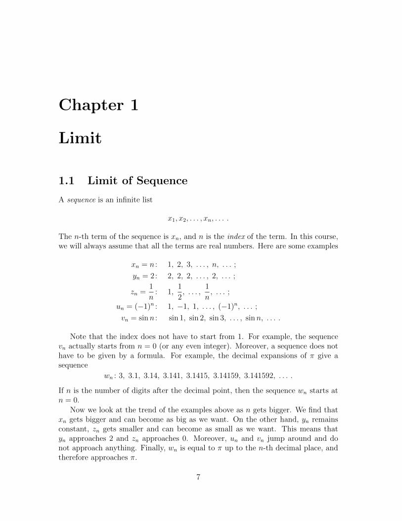
A sequence is an infinite list
x1, x2, . . . , xn, . . . .
The n-th term of the sequence is xn, and n is the index of the term. In this course,we will always assume that all the terms are real numbers. Here are some examples
xn = n : 1, 2, 3, . . . , n, . . . ;
yn = 2: 2, 2, 2, . . . , 2, . . . ;
zn =1
n: 1,
1
2, . . . ,
1
n, . . . ;
un = (−1)n : 1, −1, 1, . . . , (−1)n, . . . ;
vn = sinn : sin 1, sin 2, sin 3, . . . , sinn, . . . .
Note that the index does not have to start from 1. For example, the sequencevn actually starts from n = 0 (or any even integer). Moreover, a sequence does nothave to be given by a formula. For example, the decimal expansions of π give asequence
wn : 3, 3.1, 3.14, 3.141, 3.1415, 3.14159, 3.141592, . . . .
If n is the number of digits after the decimal point, then the sequence wn starts atn = 0.
Now we look at the trend of the examples above as n gets bigger. We find thatxn gets bigger and can become as big as we want. On the other hand, yn remainsconstant, zn gets smaller and can become as small as we want. This means thatyn approaches 2 and zn approaches 0. Moreover, un and vn jump around and donot approach anything. Finally, wn is equal to π up to the n-th decimal place, andtherefore approaches π.
7

8 CHAPTER 1. LIMIT
n
xn
yn
znun
vn
wn
Figure 1.1.1: Sequences.
Definition 1.1.1 (Intuitive). If xn approaches a finite number l when n gets biggerand bigger, then we say that the sequence xn converges to the limit l and write
limn→∞
xn = l.
A sequence diverges if it does not approach a specific finite number when n getsbigger.
The sequences yn, zn, wn converge respectively to 2, 0 and π. The sequencesxn, un, vn diverge. Since the limit describes the behavior when n gets very big, wehave the following property.
Proposition 1.1.2. If yn is obtained from xn by adding, deleting, or changing finitelymany terms, then limn→∞ xn = limn→∞ yn.
The equality in the proposition means that xn converges if and only if yn con-verges. Moreover, the two limits have equal value when both converge.
Example 1.1.1. The sequence1√n+ 2
is obtained from1√n
by deleting the first
two terms. By limn→∞1√n
= 0 and Proposition 1.1.2, we get limn→∞1√n
=
limn→∞1√n+ 2
= 0.
In general, we have limn→∞ xn+k = limn→∞ xn for any integer k.
The example assumes limn→∞1√n
= 0, which is supposed to be intuitively obvi-
ous. Although mathematics is inspired by intuition, a critical feature of mathematicsis rigorous logic. This means that we need to be clear what basic facts are assumedin any argument. For the moment, we will always assume that we already know

1.1. LIMIT OF SEQUENCE 9
limn→∞ c = c and limn→∞1
np= 0 for p > 0. After the two limits are rigorously
established in Examples 1.2.2 and 1.2.3, the conclusions based on the two limitsbecome solid.
1.1.1 Arithmetic Rule
Intuitively, if x is close to 3 and y is close to 5, then the arithmetic combinationsx+y and xy are close to 3+5 = 8 and 3 ·5 = 15. The intuition leads to the followingproperty of limit.
Proposition 1.1.3 (Arithmetic Rule). Suppose limn→∞ xn = l and limn→∞ yn = k.Then
limn→∞
(xn + yn) = l + k, limn→∞
cxn = cl, limn→∞
xnyn = kl, limn→∞
xnyn
=l
k,
where c is a constant and k 6= 0 in the last equality.
The proposition says limn→∞(xn + yn) = limn→∞ xn + limn→∞ yn. However, theequality is of different nature from the equality in Proposition 1.1.2, because theconvergence of the limits on two sides are not equivalent: If the two limits on theright converge, then the limit on the left also converges and the two sides are equal.However, for xn = (−1)n and yn = (−1)n+1, the limit limn→∞(xn + yn) = 0 on theleft converges, but both limits on the right diverge.
Exercise 1.1.1. Explain that limn→∞ xn = l if and only if limn→∞(xn − l) = 0.
Exercise 1.1.2. Suppose xn and yn converge. Explain that limn→∞ xnyn = 0 implies eitherlimn→∞ xn = 0 or limn→∞ yn = 0. Moreover, explain that the conclusion fails if xn andyn are not assumed to converge.
Example 1.1.2. We have
limn→∞
2n2 + n
n2 − n+ 1= lim
n→∞
2 +1
n
1− 1
n+
1
n2
=
limn→∞
(2 +
1
n
)limn→∞
(1− 1
n+
1
n2
)
=limn→∞ 2 + limn→∞
1
n
limn→∞ 1− limn→∞1
n+ limn→∞
1
n· limn→∞
1
n
=2 + 0
1− 0 + 0 · 0= 2.

10 CHAPTER 1. LIMIT
The arithmetic rule is used in the second and third equalities. The limits limn→∞ c =
c and limn→∞1
n= 0 are used in the fourth equality.
Exercise 1.1.3. Find the limits.
1.n+ 2
n− 3.
2.n+ 2
n2 − 3.
3.2n2 − 3n+ 2
3n2 − 4n+ 1.
4.n3 + 4n2 − 2
2n3 − n+ 3.
5.(n+ 1)(n+ 2)
2n2 − 1.
6.2n2 − 1
(n+ 1)(n+ 2).
7.(n2 + 1)(n+ 2)
(n+ 1)(n2 + 2).
8.(2− n)3
2n3 + 3n− 1.
9.(n2 + 3)3
(n3 − 2)2.
Exercise 1.1.4. Find the limits.
1.
√n+ 2√n− 3
.
2.
√n+ 2
n− 3.
3.2√n− 3n+ 2
3√n− 4n+ 1
.
4.3√n+ 4
√n− 2
2 3√n− n+ 3
.
5.(√n+ 1)(
√n+ 2)
2n− 1.
6.2n− 1
(√n+ 1)(
√n+ 2)
.
7.(√n+ 1)(n+ 2)
(n+ 1)(√n+ 2)
.
8.(2− 3
√n)3
2 3√n+ 3n− 1
.
9.( 3√n+ 3)3
(√n− 2)2
.
Exercise 1.1.5. Find the limits.
1.n+ a
n+ b.
2.
√n+ a
n+ b.
3.n+ a
n2 + bn+ c.
4.
√n+ a
n+ b√n+ c
.
5.(√n+ a)(
√n+ b)
cn+ d.
6.cn+ d
(√n+ a)(
√n+ b)
.
7.an3 + b
(c√n+ d)6
.
8.(a 3√n+ b)2
(c√n+ d)3
.
9.(a√n+ b)2
(c 3√n+ d)3
.
Exercise 1.1.6. Show that
limn→∞
apnp + ap−1n
p−1 + · · ·+ a1n+ a0
bqnq + bq−1nq−1 + · · ·+ b1n+ b0=
0, if 0 < p < q,apbq, if 0 < p = q and bq 6= 0.
Exercise 1.1.7. Find the limits.
1.1010n
n2 − 10. 2.
55(2n+ 1)2 − 1010
10n2 − 5. 3.
55(2√n+ 1)2 − 1010
10n− 5.
Exercise 1.1.8. Find the limits.

1.1. LIMIT OF SEQUENCE 11
1.n
n+ 1− n
n− 1.
2.n2
n+ 1− n2
n− 1.
3.n√n+ 1
− n√n− 1
.
4.n+ a
n+ b− n+ c
n+ d.
5.n2 + a
n+ b− n2 + c
n+ d.
6.n+ a√n+ b
− n+ c√n+ d
.
7.n3 + a
n2 + b− n3 + c
n2 + d.
8.n2 + a
n3 + b− n2 + c
n3 + d.
9.
√n+ a
3√n+ b
−√n+ c
3√n+ d
.
Exercise 1.1.9. Find the limits.
1.n2 + a1n+ a0
n+ b− n2 + c1n+ c0
n+ d.
2.n2 + a1n+ a0
n2 + b1n+ b0− n2 + c1n+ c0
n2 + d1n+ d0.
3.
(n+ a
n+ b
)2
−(n+ c
n+ d
)2
.
4.
(n2 + a
n+ b
)2
−(n2 + c
n+ d
)2
.
Exercise 1.1.10. Find the limits, p, q > 0.
1.np + a
nq + b.
2.anp + bnq + c
anq + bnp + c.
3.np + a
nq + b− np + c
nq + d.
4.n2p + a1n
p + a2
n2q + b1nq + b2.
1.1.2 Sandwich Rule
The following property reflects the intuition that if x and z are close to 3, thenanything between x and z should also be close to 3.
Proposition 1.1.4 (Sandwich Rule). Suppose xn ≤ yn ≤ zn for sufficiently big n. Iflimn→∞ xn = limn→∞ zn = l, then limn→∞ yn = l.
Note that something holds for sufficiently big n is the same as something failsfor only finitely many n.
Example 1.1.3. By 2n − 3 > n for sufficiently big n (in fact, n > 3 is enough), wehave
0 <1√
2n− 3<
1√n.
Then by limn→∞ 0 = limn→∞1√n
= 0 and the sandwich rule, we get limn→∞1√
2n− 3=
0.On the other hand, for sufficiently big n, we have n + 1 < 2n and n − 1 >
n
2,
and therefore
0 <
√n+ 1
n− 1<
√2nn
2
=2√
2√n.

12 CHAPTER 1. LIMIT
By limn→∞2√
2√n
= 2√
2 limn→∞1√n
= 0 (arithmetic rule used) and the sandwich
rule, we get limn→∞
√n+ 1
n− 1= 0.
Example 1.1.4. By −1 ≤ sinn ≤ 1, we have
− 1
n≤ sinn
n≤ 1
n,
1√n+ 1
≤ 1√n+ sinn
≤ 1√n− 1
.
By limn→∞1
n= 0, − limn→∞
1
n= 0 and the sandwich rule, we get limn→∞
sinn
n= 0.
Moreover, by limn→∞1√n+ 1
= limn→∞1√n− 1
= 0 (see argument in Example
1.1.1) and the sandwich rule, we get limn→∞1√
n+ sinn= 0.
Exercise 1.1.11. Prove that limn→∞ |xn| = 0 implies limn→∞ xn = 0.
Exercise 1.1.12. Find the limits, a > 0.
1.1√
3n− 4. 2.
√2n+ 3
4n− 1. 3.
1√an+ b
. 4.
√an+ b
cn+ d.
Exercise 1.1.13. Find the limits.
1.cosn
n.
2.(−1)n
n.
3.sin√n
n.
4.cosn√n− 2
.
5.1
n+ (−1)n.
6.cosn
n+ (−1)n.
7.cosn√
n+ (−1)n2.
8.cosn√
n+ sin√n
.
9.(−1)n√n+ (−1)n
.
10.2 + (−1)n3
3√n2 − 2 cosn
.
11.sinn+ (−1)n cosn√
n+ (−1)n.
12.| sinn+ cosn|
n.
13.3√n+ 2
2n+ (−1)n3.
14.
√n sinn+ cosn
n− 1.
15.n+ sin
√n
n+ cos 2n.
16.
√n+ sinn√n− cosn
.
17.(−1)n(n+ 1)
n2 + (−1)n+1.
18.(−1)n(n+ 10)2 − 1010
10(−1)nn2 − 5.
Exercise 1.1.14. Find the limits.
1.1. LIMIT OF SEQUENCE 13
1.
√n+ a
n+ (−1)nb.
2.1
3√n2 + an+ b
.
3.
√n+ c+ d
3√n2 + an+ b
.
4.n+ (−1)na
n+ (−1)nb.
5.(−1)n(an+ b)
n2 + c(−1)n+1n+ d.
6.(−1)n(an+ b)2 + c
(−1)nn2 + d.
7.cos√n+ a
n+ b sinn.
8.cos√n+ a√
n+ b sinn.
9.an+ b sinn
cn+ d sinn.
Exercise 1.1.15. Find the limits, p > 0.
1.sin√n
np. 2.
sin(n+ 1)
np + (−1)n. 3.
a sinn+ b
np + c. 4.
a cos(sinn)
np − b sinn.
Example 1.1.5. For a > 0, the sequence√n+ a−
√n satisfies
0 <√n+ a−
√n =
(√n+ a−
√n)(√n+ a+
√n)√
n+ a+√n
=a√
n+ a+√n<
a√n.
By limn→∞a√n
= 0 and the sandwich rule, we get limn→∞(√n+ a −
√n) = 0. Similar
argument also shows the limit for a < 0.
Example 1.1.6. The sequence
√n+ 2
nsatisfies
1 <
√n+ 2
n<n+ 2
n= 1 + 2
1
n.
By limn→∞
(1 + 2
1
n
)= 1 + 2 · 0 = 1 and the sandwich rule, we get limn→∞
√n+ 2
n= 1.
Exercise 1.1.16. Show that limn→∞(√n+ a−
√n) = 0 for a < 0.
Exercise 1.1.17. Use the idea of Example 1.1.5 to estimate
√n+ 2
n− 1 and then find
limn→∞
√n+ 2
n.
Exercise 1.1.18. Show that limn→∞
√n+ a
n+ b= 1. You may need separate argument for
a > b and a < b.
Exercise 1.1.19. Find the limits.
1.√n+ a−
√n+ b. 2.
√n+ a
√n+ c+
√n+ d
.

14 CHAPTER 1. LIMIT
3.
√n+ a+
√n+ b
√n+ c+
√n+ d
.
4.
√n+ a
√n+ b
√n+ c
√n+ d
.
5.
√n+ a+ b√n+ c+ d
.
6.√n(√n+ a−
√n+ b).
7.√n+ c(
√n+ a−
√n+ b).
8.√n+ a+
√n+ b− 2
√n+ c.
9.
√n
n2 + n+ 1.
10.
√n+ a
n2 + bn+ c.
11.√n2 + an+ b−
√n2 + cn+ d.
12.√n+ a
√n+ b−
√n+ c
√n+ d.
13.n√
n2 + n+ 1.
14.n+ a√
n2 + bn+ c.
15.
√n2 + an+ b
n2 + cn+ d.
Exercise 1.1.20. Find the limits.
1.√n+ a sinn−
√n+ b cosn.
2.
√n+ a sinn
n+ b cosn.
3.
√n+ (−1)na
n+ (−1)nb.
4.
√n+ a+ sinn√n+ c+ (−1)n
.
5.√n+ (−1)n(
√n+ a−
√n+ b).
6.√n2 + an+ sinn−
√n2 + bn+ cosn.
7.
√n2 + an+ sinn
n2 + bn+ cosn.
8.
√n2 + an+ b
n+ (−1)nc.
Exercise 1.1.21. Find the limits.
1. 3√n+ a− 3
√n+ b.
2. 3
√n+ a
n+ b.
3.3√n2( 3√n+ a− 3
√n+ b).
4. 3√n( 3√√
n+ a− 3√√
n+ b).
Exercise 1.1.22. Find the limits.
1.
(n− 2
n+ 1
)5
. 2.
(n− 2
n+ 1
)5.4
. 3.
(n− 2
n+ 1
)−√2
. 4.
(n+ a
n+ b
)p.
Exercise 1.1.23. Find the limits.
1.
( √n+ a sinn√n+ b cos 2n
)p. 2.
(n2 + an+ b
n2 + (−1)nc
)p. 3.
(n+ a
n2 + bn+ c
)p.
Exercise 1.1.24. Suppose limn→∞ xn = 1. Use the arithmetic rule and the sandwich ruleto prove that, if xn ≤ 1, then limn→∞ x
pn = 1. Of course we expect the condition xn ≤ 1
to be unnecessary. See Example 1.1.21.

1.1. LIMIT OF SEQUENCE 15
1.1.3 Some Basic Limits
Using limn→∞1
n= 0 and the sandwich rule, we may establish some basic limits.
Example 1.1.7. We show that
limn→∞
n√a = 1, for a > 0.
First assume a ≥ 1. Then xn = n√a− 1 ≥ 0, and
a = (1 + xn)n = 1 + nxn +n(n− 1)
2x2n + · · ·+ xnn > nxn.
This implies
0 ≤ xn <a
n.
By the sandwich rule and limn→∞a
n= 0, we get limn→∞ xn = 0. Then by the
arithmetic rule, this further implies
limn→∞
n√a = lim
n→∞(xn + 1) = lim
n→∞xn + 1 = 1.
For the case 0 < a ≤ 1, let b =1
a≥ 1. Then by the arithmetic rule,
limn→∞
n√a = lim
n→∞
1n√b
=1
limn→∞n√b
=1
1= 1.
Example 1.1.8. Example 1.1.7 can be extended to
limn→∞
n√n = 1.
Let xn = n√n − 1. Then we have xn > 0 for sufficiently large n (in fact, n ≥ 2 is
enough), and
n = (1 + xn)n = 1 + nxn +n(n− 1)
2x2n + · · ·+ xnn >
n(n− 1)
2x2n.
This implies
0 ≤ xn <
√2√
n− 1.
By limn→∞
√2√
n− 1= 0 (see Example 1.1.1 or 1.1.3) and the sandwich rule, we get
limn→∞ xn = 0. This further implies
limn→∞
n√n = lim
n→∞xn + 1 = 1.
16 CHAPTER 1. LIMIT
Example 1.1.9. The following “n-th root type” limits can be compared with thelimits in Examples 1.1.7 and 1.1.8
1 < n√n+ 1 <
n√
2n =n√
2 n√n,
1 < n1
n+1 < n√n,
1 < (n2 − n)n
n2−1 < (n2)n
n2/2 = ( n√n)4.
By Examples 1.1.7, 1.1.8 and the arithmetic rule, the sequences on the right convergeto 1. Then by the sandwich rule, we get
limn→∞
n√n+ 1 = lim
n→∞n
1n+1 = lim
n→∞(n2 − n)
nn2−1 = 1.
Example 1.1.10. We have
3 =n√
3n < n√
2n + 3n < n√
3n + 3n = 3n√
2.
By Example 1.1.7, we have limn→∞ 3 n√
2 = 3. Then by the sandwich rule, we getlimn→∞
n√
2n + 3n = 3.For another example, we have
3n > 3n − 2n = 3n−1 + 2 · 3n−1 − 2 · 2n−1 > 3n−1.
Taking the n-th root, we get
3 > n√
3n − 2n > 31n√
3.
By limn→∞ 31n√
3= 3 and the sandwich rule, we get limn→∞
n√
3n − 2n = 3.
Exercise 1.1.25. Prove that if a ≤ xn ≤ b for some constants a, b > 0 and sufficiently bign, then limn→∞ n
√xn = 1.
Exercise 1.1.26. Find the limits, a > 0.
1. n1
2n .
2. n2n .
3. ncn .
4. (n+ 1)cn .
5. (an+ b)cn .
6. (an2 + b)cn .
7. (√n+ 1)
cn .
8. (n− 2)1
n+3 .
9. (an+ b)c
n+d .
10. (an+ b)cn
n2+dn+e .
11. (an2 + b)c
n+d .
12. (an2 + b)cn+d
n2+en+f .
Exercise 1.1.27. Find the limits, a > 0.

1.1. LIMIT OF SEQUENCE 17
1. n√n+ sinn.
2. n√an+ b sinn.
3. n√n+ (−1)n sinn.
4. n√an+ (−1)nb sinn.
5. (n− cosn)1
n+sinn .
6. (an+ b sinn)n
n2+c cosn .
Exercise 1.1.28. Find the limits, p, q > 0.
1. n√np + sinn. 2. n
√np + nq. 3. n+2
√np + nq. 4. n−2
√np + nq.
Exercise 1.1.29. Find the limits.
1. n√
5n − 4n.
2. n√
5n − 3 · 4n.
3. n√
5n − 3 · 4n + 2n.
4. n√
5n − 3 · 4n − 2n.
5. n√
42n−1 − 5n.
6. n√
42n−1 + (−1)n5n.
7. (5n − 4n)1
n+1 .
8. (5n − 4n)1
n−2 .
9. (5n − 4n)n+1
n2+1 .
Exercise 1.1.30. Find the limits, a > b > 0.
1. n√an + bn.
2. n√an − bn.
3. n√an + (−1)nbn.
4.n√anb2n+1.
5. n+2√an + bn.
6. n−2√an − bn.
7. (an + bn)n
n2−1 .
8. (an − bn)n
n2−1 .
9. (an − (−1)nbn)n
n2−1 .
Exercise 1.1.31. For a, b, c > 0, find limn→∞n√an + bn + cn.
Exercise 1.1.32. For a ≥ 1, prove limn→∞ n√a = 1 by using
a− 1 = ( n√a− 1)
(( n√a)n−1 + ( n
√a)n−2 + · · ·+ n
√a+ 1
).
Example 1.1.11. We show that
limn→∞
an = 0, for |a| < 1.
First assume 0 < a < 1 and write a =1
1 + b. Then b > 0 and
0 < an =1
(1 + b)n=
1
1 + nb+n(n− 1)
2b2 + · · ·+ bn
<1
nb.
By limn→∞1
nb= 0 and the sandwich rule, we get limn→∞ a
n = 0.
If −1 < a < 0, then 0 < |a| < 1 and limn→∞ |an| = limn→∞ |a|n = 0. By Exercise1.1.11, we get limn→∞ a
n = 0.
Example 1.1.12. Example 1.1.11 can be extended to
limn→∞
nan = 0, for |a| < 1.

18 CHAPTER 1. LIMIT
This follows from
0 < nan =n
(1 + b)n=
n
1 + nb+n(n− 1)
2b2 + · · ·+ bn
<n
n(n− 1)
2b2
=2
(n− 1)b2,
the limit limn→∞2
(n− 1)b2= 0 and the sandwich rule.
Exercise 1.1.58 gives further extension of the limit.
Example 1.1.13. We show that
limn→∞
an
n!= 0, for any a
for the special case a = 4. For n > 4, we have
0 <4n
n!=
4 · 4 · 4 · 41 · 2 · 3 · 4
· 4
5· 4
6· · · 4
n≤ 4 · 4 · 4 · 4
1 · 2 · 3 · 4· 4
n=
45
4!
1
n.
By limn→∞45
4!
1
n= 0 and the sandwich rule, we get limn→∞
4n
n!= 0.
Exercise 1.1.59 suggests how to show the limit in general.
Exercise 1.1.33. Show that limn→∞ n2an = 0 for |a| < 1 in two ways. The first is by using
the ideas from Examples 1.1.11 and 1.1.12. The second is by using limn→∞ nan = 0 for
|a| < 1.
Exercise 1.1.34. Show that limn→∞ n5.4an = 0 for |a| < 1. What about limn→∞ n
−5.4an?What about limn→∞ n
pan?
Exercise 1.1.35. Show that limn→∞an
n!= 0 for a = 5.4 and a = −5.4.
Exercise 1.1.36. Show that limn→∞an√n!
= 0 for a = 5.4 and a = −5.4.
Exercise 1.1.37. Show that limn→∞n!an
(2n)!= 0 for any a.
Exercise 1.1.38. Find the limits.
1.n+ 1
2n.
2.n2
2n.
3. n990.99n.
4.(n2 + 1)1001
1.001n−2.
5.n+ 2n
3n.
6.n2n + (−3)n
4n.
7.n3n
(1 + 2n)2.
8.5n − n6n+1
32n−1 − 23n+1.
Exercise 1.1.39. Find the limits. Some convergence depends on a and p. You may trysome special values of a and p first.

1.1. LIMIT OF SEQUENCE 19
1. npan.
2.an
np.
3.np
an.
4.1
npan.
5.np
n!.
6.npan
n!.
7.np
n!an.
8.np√n!
.
9.npan√n!
.
10.npan
3√n!
.
11.n!an
(2n)!.
12.n!npan
(2n)!.
Exercise 1.1.40. Find the limits.
1.n2 + 3n+ 5n
n!.
2.n2 + 3n+ 5n
n!− n2 + 2n.
3.n2 + n3n + 5!
n!.
4.n23n+5 + 5 · (n− 1)!
(n+ 1)!.
5.n2 + n! + (n− 1)!
3n − n! + (n− 1)!.
6.2nn! + 3n(n− 1)!
4n(2n− 1)!− 5nn!.
Exercise 1.1.41. Prove n√n! >
√n
2. Then use this to prove limn→∞
1n√n!
= 0.
Exercise 1.1.42. Proven!
nn<
1
nand
(n!)2
(2n)!<
1
n+ 1for n > 2. Then use this to prove
limn→∞n!
nn= limn→∞
(n!)2
(2n)!= 0. What about limn→∞
(n!)k
(kn)!where k ≥ 2 is an integer?
1.1.4 Order Rule
The following property reflects the intuition that bigger sequence should have biggerlimit.
Proposition 1.1.5 (Order Rule). Suppose limn→∞ xn = l and limn→∞ yn = k.
1. If xn ≤ yn for sufficiently big n, then l ≤ k.
2. If l < k, then xn < yn for sufficiently big n.
By taking yn = l, we get the following special cases of the property for a con-verging sequence xn.
1. If xn ≤ l for sufficiently big n, then limn→∞ xn ≤ l.
2. If limn→∞ xn < l, then xn < l for sufficiently big n.
Similar statements with reversed inequalities also hold (see Exercise 1.1.43).Note the non-strict inequality in the first statement of Proposition 1.1.5 and the
strict inequality the second statement. For example, we have xn =1
n2< yn =
1
n,
but limn→∞ xn 6< limn→∞ yn. The example also satisfies limn→∞ xn ≥ limn→∞ ynbut xn 6≥ yn, even for sufficiently big n.

20 CHAPTER 1. LIMIT
Exercise 1.1.43. Explain how to get the following special cases of the order rule.
1. If xn ≥ l for sufficiently big n, then limn→∞ xn ≥ l.
2. If limn→∞ xn > l, then xn > l for sufficiently big n.
Example 1.1.14. By limn→∞2n2 + n
n2 − n+ 1= 2 and the order rule, we know 1 <
2n2 + n
n2 − n+ 1< 3 for sufficiently big n. This implies 1 < n
√2n2 + n
n2 − n+ 1< n√
3 for
sufficiently big n. By limn→∞n√
3 = 1 and the sandwich rule, we get
limn→∞
n
√2n2 + n
n2 − n+ 1= 1.
Example 1.1.15. We showed limn→∞n√
3n − 2n = 3 in Example 1.1.10. Here we usea different method, with the help of the order rule.
By n√
3n − 2n = 3 n
√1−
(2
3
)n, we only need to find limn→∞
n
√1−
(2
3
)n. By
Example 1.1.11, we have limn→∞
(1−
(2
3
)n)= 1. By the order rule, therefore,
we have1
2< 1−
(2
3
)n< 2
for sufficiently big n. This implies that
1n√
2< n
√1−
(2
3
)n<
n√
2
for sufficiently big n. Then by Example 1.1.7 and the sandwich rule, we get
limn→∞n
√1−
(2
3
)n= 1, and we conclude that
limn→∞
n√
3n − 2n = 3 limn→∞
n
√1−
(2
3
)n= 3.
Exercise 1.1.44. Prove that if limn→∞ xn = l > 0, then limn→∞ n√xn = 1. Moreover, find
a sequence satisfying limn→∞ xn = 0 and limn→∞ n√xn = 1. Can we have xn converging
to 0 and n√xn converging to 0.32?
Exercise 1.1.45. Find the limits.

1.1. LIMIT OF SEQUENCE 21
1. n√
5n − n4n.
2. n+2√
5n − n4n.
3. n−2√
5n − n4n.
4. n√
5n − (−1)nn4n.
5. (5n − n4n)n−1
n2+1 .
6. (5n−(−1)nn4n)n+(−1)n
n2+1 .
Exercise 1.1.46. Find the limits.
1. n
√1
n5n − n4n.
2. n
√1
n5n − (−1)nn4n.
3. n+2
√1
n5n − n4n sinn.
4. (n242n−1 − 5n)n−1
n2+1 .
5.n
√n2n + 4n+1 +
3n−1
n.
6.n−2
√n23n +
32n−1
n2.
7. n−2
√23n +
n− 1
n2 + 132n−1.
8.
(n23n +
32n−1
n2
)n−1
n2
.
9.
(n23n +
32n−1
n2
) 1n2
.
Exercise 1.1.47. Find the limits, a > b.
1. n√an+1 + bn.
2. n√an+1 + (−1)nbn.
3. n−2√an+1 + (−1)nbn.
4. n√
4an − 5bn.
5. n√
4an + 5b2n+1.
6. n√a+ bn.
7. n√an+ bn.
8. n−2√nan + (n2 + 1)bn.
9. n+2
√1
nan + nbn+1.
10. (an + bn)n+1
n2+1 .
11. ((n+ 1)an + bn)n
n2−1 .
12. (an + bn)1
n2−1 .
13. (an + (−1)nbn)(−1)n
n2−1 .
Exercise 1.1.48. Find the limits, a, b, c > 0.
1. n√n2an + nbn + 2cn.
2. n√an(bn + 1) + ncn.
3. n√
(n+ sinn)an + bn + n2cn.
4. n√an(n+ bn(1 + ncn)).
Exercise 1.1.49. Suppose a polynomial p(n) = apnp+an−1n
p−1 + · · ·+a1n+a0 has leadingcoefficient ap > 0. Prove that p(n) > 0 for sufficiently big n.
Exercise 1.1.50. Suppose a, b, c > 0, and p, q, r are polynomials with positive leading coef-ficients. Find the limit of n
√p(n)an + q(n)bn + r(n)cn.
Exercise 1.1.51. Find the limits, a, b, p, q > 0.
1. n√anp + b sinn.
2. n√anp + bnq.
3. n+2√anp + bnq.
4. n−2√anp + bnq.
5. n2√anp + bnq.
6. (anp + bnq)1
n2−1 .

22 CHAPTER 1. LIMIT
Example 1.1.16. The sequence xn =3n(n!)2
(2n)!satisfies
limn→∞
xnxn−1
= limn→∞
3n2
2n(2n− 1)=
3
4= 0.75.
By the order rule, we havexnxn−1
< 0.8 for sufficiently big n, say for n > N (in fact,
N = 8 is enough). Then for n > N , we have
0 < xn =xnxn−1
xn−1
xn−2
· · · xN+1
xNxN < 0.8n−NxN = C · 0.8n, C = 0.8−NxN .
By Example 1.1.11, we have limn→∞ 0.8n = 0. Since C is a constant, by the sandwichrule, we get limn→∞ xn = 0.
Exercises 1.1.52 and 1.1.53 summarise the idea of the example.
Exercise 1.1.52. Prove that if
∣∣∣∣ xnxn−1
∣∣∣∣ ≤ c for a constant c < 1, then xn converges to 0.
Exercise 1.1.53. Prove that if limn→∞xnxn−1
= l and |l| < 1, then xn converges to 0.
Exercise 1.1.54. Find a such that the sequence converges to 0, p, q > 0.
1.(2n)!
(n!)2an.
2.(n!)2
(3n)!an.
3.(n!)3
(3n)!an.
4.
√(2n)!
n!an.
5.√n!an
2.
6.an
2
n!.
7.an
2
√n!
.
8. (n!)pan.
9.an
(n!)p.
10.nqan
(n!)p.
11.(n!)p
((2n)!)qan.
12.n5(n!)p
((2n)!)qan.
1.1.5 Subsequence
A subsequence is obtained by choosing infinitely many terms from a sequence. Wedenote a subsequence by
xnk : xn1 , xn2 , . . . , xnk , . . . ,
where the indices satisfy
n1 < n2 < · · · < nk < · · · .The following are some examples
x2k : x2, x4, x6, x8, . . . , x2k, . . . ,
x2k−1 : x1, x3, x5, x7, . . . , x2k−1, . . . ,
x2k : x2, x4, x8, x16, . . . , x2k , . . . ,
xk! : x1, x2, x6, x24, . . . , xk!, . . . .

1.1. LIMIT OF SEQUENCE 23
If xn starts at n = 1, then n1 ≥ 1, which further implies nk ≥ k for all k.
Proposition 1.1.6. If a sequence converges to l, then any subsequence convergesto l. Conversely, if a sequence is the union of finitely many subsequences that allconverge to the same limit l, then the whole sequence converges to l.
Example 1.1.17. Since1
n2is a subsequence of
1
n, limn→∞
1
n= 0 implies limn→∞
1
n2=
0. We also know limn→∞1√n
= 0 implies limn→∞1
n= 0 but not vice versa.
Example 1.1.18. The sequencen+ (−1)n3
n− (−1)n2is the union of the odd subsequence
(2k − 1)− 3
(2k − 1) + 2=
2k − 4
2k + 1and the even subsequence
2k + 3
2k − 2. Both subsequences con-
verge to 1, either by direct computation, or by regarding them also as subsequences
ofn− 4
n+ 1and
n+ 3
n− 2, which converge to 1. Then we conclude limn→∞
n+ (−1)n3
n− (−1)n2= 1.
Example 1.1.19. The sequence (−1)n has one subsequence (−1)2k = 1 converging to1 and another subsequence (−1)2k−1 = −1 converging to −1. Since the two limitsare different, by Proposition 1.1.6, the sequence (−1)n diverges.
Example 1.1.20. The sequence sinna converges to 0 when a is an integer multiple ofπ. Now assume 0 < a < π. For any natural number k, the interval [kπ, (k + 1)π]of length π contains the following interval of length a (both intervals have the samemiddle point)
[ak, bk] =
[kπ +
π − a2
, (k + 1)π − π − a2
].
For even k, we have sinx ≥ sin
(π − a
2
)= cos
a
2> 0 on [ak, bk]. For odd k, we
have sinx ≤ − cosa
2< 0 on [ak, bk].
Since the arithmetic sequence a, 2a, 3a, . . . has increment a, which is the lengthof [ak, bk], we must have nka ∈ [ak, bk] for some natural number nk. Then sinn2ka is a
subsequence of sinna satisfying sinn2k ≥ cosa
2> 0, and sinn2k+1a is a subsequence
satisfying sinn2k ≤ − cosa
2. Therefore the two subsequences cannot converge to the
same limit. As a result, the sequence sinna diverges.
Now for general a that is not an integer multiple of π, we have a = 2Nπ ± b foran integer N and b satisfying 0 < b < π. Then we have sinna = ± sinnb. We haveshown that sinnb diverges, so that sinna diverges.
We conclude that sinna converges if and only if a is an integer multiple of π.

24 CHAPTER 1. LIMIT
Exercise 1.1.55. Find the limit.
1.√n! + 1−
√n!− 1.
2. (n!)1n! .
3. ((n+ 1)!)1n! .
4. ((n+ (−1)n)!)1n! .
5. (n!)1
(n+1)! .
6. (2n2−1 + 3n
2)
1n2 .
Exercise 1.1.56. Explain convergence or divergence.
1. 2(−1)n .
2. n(−1)n
n .
3. n(−1)n .
4.(−1)nn+ 3
n− (−1)n2.
5.(−1)nn2
n3 − 1.
6.√n(√
n+ (−1)n −√n)
.
7. (2(−1)nn + 3n)1n .
8. (2n + 3(−1)nn)1n .
9. tannπ
3.
10. (−1)n sinnπ
3.
11. sinnπ
2cos
nπ
3.
12.n sin
nπ
3
n cosnπ
2+ 2
.
13.n− sin
nπ
3
n+ 2 cosnπ
2
.
Exercise 1.1.57. Find all a such that the sequence cosna converges.
Example 1.1.21. We prove that limn→∞ xn = 1 implies limn→∞ xpn = 1. Exercises
1.1.58 and 1.1.59 extend the result.The sequence xn is the union of two subsequences x′k and x′′k (short for xmk and
xnk) satisfying all x′k ≥ 1 and all x′′k ≤ 1. By Proposition 1.1.6, the assumptionlimn→∞ xn = 1 implies that limk→∞ x
′k = limk→∞ x
′′k = 1.
Pick integers M and N satisfying M < p < N . Then x′k ≥ 1 implies x′kM ≤
x′kp ≤ x′k
N . By the arithmetic rule, we have limk→∞ x′kM = (limk→∞ x
′k)M = 1M = 1
and similarly limk→∞ x′kN = 1. Then by the sandwich rule, we get limk→∞ x
′kp = 1.
Similar proof shows that limk→∞ x′′kp = 1. Since the sequence xpn is the union of
two subsequences x′kp and x′′k
p, by Proposition 1.1.6 again, we get limn→∞ xpn = 1.
Exercise 1.1.58. Suppose limn→∞ xn = 1 and yn is bounded. Prove that limn→∞ xynn = 1.
Exercise 1.1.59. Suppose limn→∞ xn = l > 0. By applying Example 1.1.21 to the sequencexnl
, prove that limn→∞ xpn = lp.
1.2 Rigorous Definition of Sequence Limit
The statement limn→∞1
n= 0 means that
1
ngets smaller and smaller as n gets
bigger and bigger. To make the statement rigorous, we need to be more specificabout smaller and bigger.
Is 1000 big? The answer depends on the context. A village of 1000 people isbig, and a city of 1000 people is small (even tiny). Similarly, a rope of diameter less

1.2. RIGOROUS DEFINITION OF SEQUENCE LIMIT 25
than one millimeter is considered thin. But the hair is considered thin only if thediameter is less than 0.05 millimeter.
So big or small makes sense only when compared with some reference quantity.We say n is in the thousands if n > 1000 and in the millions if n > 10000000.The reference quantities 1000 and 1000000 give a sense of the scale of bigness. In
this spirit, the statement limn→∞1
n= 0 means the following list of infinitely many
implications
n > 1 =⇒∣∣∣∣ 1n − 0
∣∣∣∣ < 1,
n > 10 =⇒∣∣∣∣ 1n − 0
∣∣∣∣ < 0.1,
n > 100 =⇒∣∣∣∣ 1n − 0
∣∣∣∣ < 0.01,
...
n > 1000000 =⇒∣∣∣∣ 1n − 0
∣∣∣∣ < 0.000001,
...
For another example, limn→∞2n
n!= 0 means the following implications
n > 10 =⇒∣∣∣∣2nn!− 0
∣∣∣∣ < 0.0003,
n > 20 =⇒∣∣∣∣2nn!− 0
∣∣∣∣ < 0.0000000000005,
...
So the general shape of the implications is
n > N =⇒ |xn − l| < ε.
Note that the relation between N (measuring the bigness of n) and ε (measuringthe smallness of |xn − l|) may be different for different limits.
The problem with infinitely many implications is that our language is finite.In practice, we cannot verify all the implications one by one. Even if we haveverified the truth of the first one million implications, there is no guarantee thatthe one million and the first implication is true. To mathematically establish thetruth of all implications, we have to formulate one finite statement that includes theconsideration for all N and all ε.

26 CHAPTER 1. LIMIT
1.2.1 Rigorous Definition
Definition 1.2.1 (Rigorous). A sequence xn converges to a finite number l, anddenoted limn→∞ xn = l, if for any ε > 0, there is N , such that n > N implies|xn − l| < ε.
In case N is a natural number (which can always be arranged if needed), thedefinition means that, for any given horizontal ε-band around l, we can find N , suchthat all the terms xN+1, xN+2, xN+3, . . . after N lie in the shaded area in Figure1.2.1.
ll + ε
l − ε
Nn
x1
x2
x3
x4
xN+1
xN+2 xN+3
xn xn+1
Figure 1.2.1: n > N implies |xn − l| < ε.
Example 1.2.1. For any ε > 0, choose N =1
ε. Then
n > N =⇒∣∣∣∣ 1n − 0
∣∣∣∣ =1
n<
1
N= ε.
This verifies the rigorous definition of limn→∞1
n= 0.
By applying the rigorous definition to ε = 0.1, 0.01, . . . , we recover the infinitelymany implications we wish to achieve. This justifies the rigorous definition of limit.
Example 1.2.2. For the constant sequence xn = c, we rigorously prove
limn→∞
c = c.
For any ε > 0, choose N = 0. Then
n > 0 =⇒ |xn − c| = |c− c| = 0 < ε.
In fact, the right side is always true, regardless of the left side.
Example 1.2.3. We rigorously prove
limn→∞
1
np= 0, for p > 0.

1.2. RIGOROUS DEFINITION OF SEQUENCE LIMIT 27
For any ε > 0, choose N =1
ε1p
. Then
n > N =⇒∣∣∣∣ 1
np− 0
∣∣∣∣ =1
np<
1
Np= ε.
We need to be more specific on the logical foundation for the arguments. Wewill assume the basic knowledge of real numbers, which are the four arithmetic
operations x + y, x − y, xy, xy
, the exponential operation xy (for x > 0), the order
x < y (or y > x, and x ≤ y means x < y or x = y), and the properties for these
operations. For example, we assume that we already know x > y > 0 implies1
x<
1
yand xp > yp for p > 0. These properties are used in the example above.
More important about the knowledge assumed above is the knowledge that arenot assumed and therefore cannot be used until after the knowledge is established.In particular, we do not assume any knowledge about the logarithm. The logarithmand its properties will be rigorously established in Example 1.7.15 as the inverse ofexponential.
Example 1.2.4. To rigorously prove limn→∞n2 − 1
n2 + 1= 1, for any ε > 0, we have
n > N =
√2
ε− 1 =⇒
∣∣∣∣n2 − 1
n2 + 1− 1
∣∣∣∣ =2
n2 + 1<
2
N2 + 1=
2(2
ε− 1
)+ 1
= ε.
Therefore the sequence converges to 1.
How did we choose N =
√2
ε− 1? We want to achieve
∣∣∣∣n2 − 1
n2 + 1− 1
∣∣∣∣ < ε. Since
this is equivalent to2
n2 + 1< ε, which we can solve to get n >
√2
ε− 1, choosing
N =
√2
ε− 1 should work.
Example 1.2.5. To rigorously prove the limit in Example 1.1.5, we estimate thedifference between the sequence and the expected limit
|√n+ 2−
√n− 0| = (n+ 2)− n√
n+ 2 +√n<
2√n.
This shows that for any ε > 0, it is sufficient to have2√n< ε, or n >
4
ε2. In other
words, we should choose N =4
ε2.

28 CHAPTER 1. LIMIT
The discussion above is the analysis of the problem, which you may write onyour scratch paper. The formal rigorous argument you are supposed to present is
the following: For any ε > 0, choose N =4
ε2. Then
n > N =⇒ |√n+ 2−
√n− 0| = 2√
n+ 2 +√n<
2√n<
2√N
= ε.
1.2.2 The Art of Estimation
In Examples 1.2.4, the formula for N is obtained by solving
∣∣∣∣n2 − 1
n2 + 1− 1
∣∣∣∣ < ε in
exact way. However, this may not be so easy in general. For example, for the limitin Example 1.1.2, we need to solve∣∣∣∣ 2n2 + n
n2 − n+ 1− 2
∣∣∣∣ =3n− 2
n2 − n+ 1< ε.
While the exact solution can be found, the formula for N is rather complicated. Formore complicated example, it may not even be possible to find the formula for theexact solution.
We note that finding the exact solution of |xn − l| < ε is the same as findingN = N(ε), such that
n > N ⇐⇒ |xn − l| < ε.
However, in order to rigorously prove the limit, only =⇒ direction is needed. Theweaker goal can often be achieved in much simpler way.
Example 1.2.6. Consider the limit in Example 1.1.2. For n > 1, we have∣∣∣∣ 2n2 + n
n2 − n+ 1− 2
∣∣∣∣ =3n− 2
n2 − n+ 1<
3n
n2 − n=
3
n− 1.
Since3
n− 1< ε implies
∣∣∣∣ 2n2 + n
n2 − n+ 1− 2
∣∣∣∣ < ε, and3
n− 1< ε is equivalent to
n >3
ε+ 1, we find that choosing N =
3
ε+ 1 is sufficient
n > N =3
ε+ 1 =⇒
∣∣∣∣ 2n2 + n
n2 − n+ 1− 2
∣∣∣∣ =3n− 2
n2 − n+ 1<
3
n− 1<
3
N − 1= ε.
Exercise 1.2.1. Show that
∣∣∣∣n2 − 1
n2 + 1− 1
∣∣∣∣ < 2
nand then rigorously prove limn→∞
n2 − 1
n2 + 1= 1.
The key for the rigorous proof of limits is to find a simple and good enoughestimation. We emphasize that there is no need to find the best estimation. Anyestimation that can fulfill the rigorous definition of limit is good enough.

1.2. RIGOROUS DEFINITION OF SEQUENCE LIMIT 29
Everyday life is full of good enough estimations. Mastering the art of suchestimations is very useful for not just learning calculus, but also for making smartjudgement in real life.
Example 1.2.7. If a bottle is 20% bigger in size than another bottle, how much biggeris in volume?
The exact formula is the cube of the comparison in size
(1 + 0.2)3 = 1 + 3 · 0.2 + 3 · 0.22 + 0.23.
Since 3 · 0.2 = 0.6, 3 · 0.22 = 0.12, and 0.23 is much smaller than 0.1, the bottle is alittle more than 72% bigger in volume.
Example 1.2.8. The 2013 GDP per capita is 9,800USD for China and 53,100USD forthe United States, in terms of PPP (purchasing power parity). The percentage ofthe annual GDP growth for the three years up to 2013 are 9.3, 7.7, 7.7 for Chinaand 1.8, 2.8, 1.9 for the United States. What do we expect the number of years forChina to catch up to the United States?
First we need to estimate how much faster is the Chinese GDP growing comparedto the United States. The comparison for 2013 is
1 + 0.077
1 + 0.019≈ 1 + (0.077− 0.019) = 1 + 0.058.
Similarly, we get the (approximate) comparisons 1 + 0.075 and 1 + 0.049 for theother two years. Among the three comparisons, we may choose a more conservative1 + 0.05. This means that we assume Chinese GDP per capita grows 5% faster thanthe United States for the next many years.
Based on the assumption of 5%, the number of years n for China to catch up tothe United States is obtained exactly by solving
(1 + 0.05)n = 1 + n 0.05 +n(n− 1)
20.052 + · · ·+ 0.05n =
53, 100
9, 800≈ 5.5.
If we use 1 + n 0.05 to approximate (1 + 0.05)n, then we get n ≈ 5.5− 1
0.05= 90.
However, 90 years is too pessimistic because for n = 90, the third termn(n− 1)
20.052
is quite sizable, so that 1 + n 0.05 is not a good approximation of (1 + 0.05)n.An an exercise for the art of estimation, we try to avoid using calculator in
getting better estimation. By53, 100
9, 800≈ 2.32, we may solve
n = 2m, (1 + 0.05)m = 1 +m 0.05 +m(m− 1)
20.052 + · · ·+ 0.05m ≈ 2.3.

30 CHAPTER 1. LIMIT
We get n ≈ 2 · 2.3− 1
0.05= 52. Since
m(m− 1)
20.052 is still sizable for m = 26 (but
giving much better approximation than n = 90), the actual n should be somewhatsmaller than 52. We try n = 40 and estimate (1 + 0.05)n by the first three terms
(1 + 0.05)40 ≈ 1 + 40 · 0.05 +40 · 39
20.052 ≈ 5.
So it looks like somewhere between 40 and 45 is a good estimation.We conclude that, if Chinese GDP per capita growth is 5% (a very optimistic
assumption) faster than the United States in the next 50 years, then China willcatch up to the United States in 40 some years.
Exercise 1.2.2. I wish to paint a wall measuring 3 meters tall and 6 meters wide, give ortake 10% in each direction. If the cost of paint is $13.5 per square meters, how muchshould I pay for the paint?
Exercise 1.2.3. In a supermarket, I bought four items at $5.95, $6.35, $15.50, $7.20. Thesales tax is 8%. The final bill is around $38. Is the bill correct?
Exercise 1.2.4. In 1900, Argentina and Canada had the same GDP per capita. In 2000,the GDP per capita is 9,300USD for Argentina and 24,000USD for Canada. On average,how much faster is Canadian GDP growing annually compared with Argentina in the 20thcentury?
Next we leave real life estimations and try some examples in calculus.
Example 1.2.9. If x is close to 3 and y is close to 5, then 2x−3y is close to 2·3−3·5 =−9. We wish to be more precise about the statement, say, we want to find a tolerancefor x and y, such that 2x− 3y is within ±0.2 of −9.
We have
|(2x− 3y)− (−9)| = |2(x− 3)− 3(y − 5)| ≤ 2|x− 3|+ 3|y − 5|.
For the difference to be within ±0.2, we only need to make sure 2|x−3|+ 3|y−5| <0.2. This can be easily achieved by |x− 3| < 0.2
2+3= 0.04 and |y − 5| < 0.04.
Example 1.2.10. Again we assume x and y are close to 3 and 5. Now we want tofind the percentage of tolerance, such that 2x− 3y is within ±0.2 of −9.
We can certainly use the answer in Example 1.2.9 and find the percentage 0.043≈
1.33% for x and 0.045≈ 0.8% for y. This implies that, if both x and y are within
0.8% of 3 and 5, then 2x− 3y is within ±0.2 of −9.The better (or more honest) way is to directly solve the problem. Let δ1 and δ2
be the percentage of tolerance for x and y. Then x = 3(1 + δ1) and y = 5(1 + δ2),and
|(2x−3y)−(−9)| = |2(x−3)−3(y−5)| ≤ |2·3δ1−3·5δ2| ≤ 21δ, δ = max{|δ1|, |δ2|}.

1.2. RIGOROUS DEFINITION OF SEQUENCE LIMIT 31
To get 21|δ| to be within our target of 0.2, we may take our tolerance δ = 0.9% <0.221≈ 0.0095.
Example 1.2.11. Assume x and y are close to 3 and 5. We want to find the tolerancefor x and y, such that xy is within ±0.2 of 3 · 5 = 15. This means finding δ > 0,such that
|x− 3| < δ, |y − 5| < δ =⇒ |xy − 15| < 0.2.
Under the assumptions |x− 3| < δ and |y − 5| < δ, we have
|xy − 15| ≤ |xy − 3y|+ |3y − 15| ≤ |x− 3||y|+ 3|y − 5| ≤ (|y|+ 3)δ.
We also note that, if we postulate δ ≤ 1, then |y− 5| < δ implies 4 < y < 6, so that
|xy − 15| ≤ (|y|+ 3)δ ≤ (6 + 3)δ = 9δ.
To get 9|δ| to be within our target of 0.2, we may take our tolerance δ = 0.02 < 0.29
.Since this indeed satisfies δ ≤ 1, we conclude that we can take δ = 0.02.
If the targeted error ±0.2 is changed to some other amount ±ε, then the sameargument shows that we can take the tolerance to be δ = ε
10. Strictly speaking,
since we also use δ ≤ 1 in the argument above, we should take δ = min{ ε10, 1}.
Exercise 1.2.5. Find a tolerance for x, y, z near −2, 3, 5, such that 5x − 3y + 4z is within±ε of 1.
Exercise 1.2.6. Find a tolerance for x and y near 2 and 2, such that xy is within ±ε of 4.
Exercise 1.2.7. Find a tolerance for x near 2, such that x2 is within ±ε of 4.
Exercise 1.2.8. Find a percentage of tolerance for x near 2, such that1
xis within ±0.1 of
0.5.
1.2.3 Rigorous Proof of Limits
We revisit the limits derived before and make the argument rigorous.
Example 1.2.12. In Example 1.1.5, we argued that limn→∞(√n+ a −
√n) = 0. To
make the argument rigorous, we use the estimation in the earlier example. In fact,regardless of the sign of a, we always have
|√n+ a−
√n− 0| =
∣∣∣∣(√n+ a−√n)(√n+ a+
√n)√
n+ a+√n
∣∣∣∣ =|a|√
n+ a+√n<|a|√n.
For the right side|a|√n< ε, it is sufficient to have n >
a2
ε2. Then we can easily get
n >a2
ε2=⇒ |
√n+ a−
√n− 0| < ε.

32 CHAPTER 1. LIMIT
This gives the rigorous proof of limn→∞(√n+ a−
√n) = 0.
Example 1.2.13. In Example 1.1.6, we argued that limn→∞
√n+ 2
n= 1. To make
the argument rigorous, we use the estimation in the earlier example. The estimation
suggested that it is sufficient to have 21
n< ε. Thus we get the following rigorous
argument for the limit
n <2
ε=⇒ 0 <
√n+ 2
n− 1 <
n+ 2
n− 1 =
2
n< ε =⇒
∣∣∣∣∣√n+ 2
n− 1
∣∣∣∣∣ < ε.
Exercise 1.2.9. Rigorously prove the limits.
1.n+ 2
n− 3.
2.n− 2
n+ 3.
3.n+ a
n+ b.
4.2n2 − 3n+ 2
3n2 − 4n+ 1.
5.
√n+ 2√n− 3
.
6.
√n+ a
n+ b.
7.n
n+ 1− n
n− 1.
8.n+ a
n+ b− n+ c
n+ d.
9.1√
an+ b.
10.sin√n
n.
11.cos√n+ a
n+ b sinn.
12.√n+ a−
√n+ b.
13.
√n+ a
n+ b.
14. 3√n+ 1− 3
√n.
Exercise 1.2.10. Rigorously prove the limits, p > 0.
1.a√
np + b. 2.
np + a
np + b. 3.
a sinn+ b
np + c.
Example 1.2.14. The estimation in Example 1.1.7 tells us that | n√a − 1| < a
nfor
a > 1. This suggests that for any ε > 0, we may choose N =a
ε. Then
n > N =⇒ | n√a− 1| < a
n<
a
N= ε.
This rigorously proves that limn→∞n√a = 1 in case a ≥ 1.
Example 1.2.15. We try to rigorously prove limn→∞ n2an = 0 for |a| < 1.
Using the idea of Example 1.1.11, we write |a| =1
1 + b. Then |a| < 1 implies

1.2. RIGOROUS DEFINITION OF SEQUENCE LIMIT 33
b > 0, and for n ≥ 3, we have
|n2an − 0| = n2|a|n =n2
(1 + b)n
=n2
1 + nb+n(n− 1)
2!b2 +
n(n− 1)(n− 2)
3!b3 + · · ·+ bn
<n2
n(n− 1)(n− 2)
3!b3
=3!n
(n− 1)(n− 2)b3<
3!nn
2
n
2b3
=3!22
nb3.
Since3!22
nb3< ε is the same as n >
3!22
b3ε, we have
n >3!22
b3εand n ≥ 3 =⇒ |n2an − 0| < 3!22
nb3< ε.
This shows that we may choose N = max
{3!22
b3ε, 3
}.
It is clear from the proof that we generally have
limn→∞
npan = 0, for any p and |a| < 1.
Example 1.2.16. We rigorously prove limn→∞an
n!= 0 in Example 1.1.13.
Choose a natural number M satisfying |a| < M . Then for n > M , we have∣∣∣∣ann!
∣∣∣∣ < Mn
n!=M ·M · · ·M
1 · 2 · · ·M· M
M + 1· M
M + 2· · ·M
n≤ MM
M !· Mn
=MM+1
M !· 1
n.
Therefore for any ε > 0, we have
n > max
{MM+1
M !ε,M
}=⇒
∣∣∣∣ann!− 0
∣∣∣∣ < MM+1
M !· 1
n<MM+1
M !· 1
MM+1
M !ε
= ε.
Exercise 1.2.11. Rigorously prove the limits.
1. n√n.
2.n5.4
n!.
3.np
n!.
4.n5.43n
n!.
5.npan
n!.
6.n!
nn.
7. npan, |a| < 1.
1.2.4 Rigorous Proof of Limit Properties
The rigorous definition of limit allows us to rigorously prove some limit properties.

34 CHAPTER 1. LIMIT
Example 1.2.17. Suppose limn→∞ xn = l > 0. We prove that limn→∞√xn =
√l.
First we clarify the problem. The limit limn→∞ xn = l means the implication
For any ε > 0, there is N , such that n > N =⇒ |xn − l| < ε.
The limit limn→∞√xn =
√l means the implication
For any ε > 0, there is N , such that n > N =⇒ |√xn −
√l| < ε.
We need to argue is that the first implication implies the second implication.We have
|√xn −
√l| =
|(√xn −√l)(√xn +
√l)|
√xn +
√l
=|xn − l|√xn +
√l≤ |xn − l|√
l.
Therefore for any given ε > 0, the second implication will hold as long as|xn − l|√
l< ε,
or |xn − l| <√lε. The inequality |xn − l| <
√lε can be achieved from the first
implication, provided we apply the first implication to√lε in place of ε.
The analysis above leads to the following formal proof. Let ε > 0. By applyingthe definition of limn→∞ xn = l to
√lε > 0, there is N , such that
n > N =⇒ |xn − l| <√lε.
Then
n > N =⇒ |xn − l| <√lε
=⇒ |√xn −
√l| =
|(√xn −√l)(√xn +
√l)|
√xn +
√l
=|xn − l|√xn +
√l≤ |xn − l|√
l< ε.
In the argument, we take advantage of the fact that the definition of limit canbe applied to any positive number,
√lε for example, instead of the given positive
number ε.
Example 1.2.18. We prove the arithmetic rule limn→∞(xn + yn) = limn→∞ xn +limn→∞ yn in Proposition 1.1.3. The concrete Example 1.2.9 provides idea of theproof.
Let limn→∞ xn = l and limn→∞ yn = k. Then for any ε1 > 0, ε2 > 0, there areN1, N2, such that
n > N1 =⇒ |xn − l| < ε1,
n > N2 =⇒ |yn − k| < ε2.
We expect to choose ε1, ε2 as some modification of ε, as demonstrated in Example1.2.17.

1.2. RIGOROUS DEFINITION OF SEQUENCE LIMIT 35
Let N = max{N1, N2}. Then
n > N =⇒ n > N1, n > N2
=⇒ |xn − l| < ε1, |yn − k| < ε2
=⇒ |(xn + yn)− (l + k)| ≤ |xn − l|+ |yn − k| < ε1 + ε2.
If ε1 + ε2 ≤ ε, then this rigorously proves limn→∞(xn + yn) = l + k. Of course this
means that we may choose ε1 = ε2 =ε
2at the beginning of the argument.
The analysis above leads to the following formal proof. For any ε > 0, apply the
definition of limn→∞ xn = l and limn→∞ yn = k toε
2> 0. We find N1 and N2, such
that
n > N1 =⇒ |xn − l| <ε
2,
n > N2 =⇒ |yn − k| <ε
2.
Then
n > max{N1, N2} =⇒ |xn − l| <ε
2, |yn − k| <
ε
2
=⇒ |(xn + yn)− (l + k)| ≤ |xn − l|+ |yn − k| <ε
2+ε
2= ε.
Example 1.2.19. The arithmetic rule limn→∞ xnyn = limn→∞ xn limn→∞ yn in Propo-sition 1.1.3 means that, if we know the approximate values of the width and heightof a rectangle, then multiplying the width and height approximates the area of therectangle. The rigorous proof requires us to estimate how the approximation of thearea is affected by the approximations of the width and height. Example 1.2.11gives the key idea for such estimation.
area= |l||y − k|
area
=|x−l||y|
l
k
x
y
Figure 1.2.2: The error in product.

36 CHAPTER 1. LIMIT
Let limn→∞ xn = l and limn→∞ yn = k. Then for any ε1 > 0, ε2 > 0, there areN1, N2, such that
n > N1 =⇒ |xn − l| < ε1,
n > N2 =⇒ |yn − k| < ε2.
Then for n > N = max{N1, N2}, we have (see Figure 1.2.2)
|xnyn − lk| = |(xn − l)yn + l(yn − k)|≤ |xn − l||yn|+ |l||yn − k|< ε1(|k|+ ε2) + |l|ε2,
where we use |yn − k| < ε2 implying |yn| < |k|+ ε2. The proof of limn→∞ xnyn = lkwill be complete if, for any ε > 0, we can choose ε1 > 0 and ε2 > 0, such that
ε1(|k|+ ε2) + |l|ε2 ≤ ε.
This can be achieved by choosing ε1, ε2 satisfying
ε2 ≤ 1, ε1(|k|+ 1) ≤ ε
2, |l|ε2 ≤
ε
2.
In other words, if we choose
ε1 =ε
2(|k|+ 1), ε2 = min
{1,
ε
2|l|
}at the very beginning of the proof, then we get a rigorous proof of the arithmeticrule. The formal writing of the proof is left to the reader.
Example 1.2.20. The sandwich rule in Proposition 1.1.4 reflects the intuition that, ifx and z are within ε of 5, then any number y between x and z is also within ε of 5
|x− 5| < ε, |z − 5| < ε, x ≤ y ≤ z =⇒ |y − 5| < ε.
Geometrically, this means that if x and z lies inside an interval, say (5 − ε, 5 + ε),then any number y between x and z also lies in the interval.
Suppose xn ≤ yn ≤ zn and limn→∞ xn = limn→∞ zn = l. For any ε > 0, there areN1 and N2, such that
n > N1 =⇒ |xn − l| < ε,
n > N2 =⇒ |zn − l| < ε.
Then
n > N = max{N1, N2} =⇒ |xn − l| < ε, |zn − l| < ε
=⇒ l − ε < xn, zn < l + ε
=⇒ l − ε < xn ≤ yn ≤ zn < l + ε
⇐⇒ |yn − l| < ε.

1.3. CRITERION FOR CONVERGENCE 37
Example 1.2.21. The order rule in Proposition 1.1.5 reflects the intuition that, if x isvery close to 3 and y is very close to 5, then x must be less than y. More specifically,we know x < y when x and y are within ±1 of 3 and 5. Here 1 is half of the distancebetween 3 and 5.
Suppose xn ≤ yn, limn→∞ xn = l, limn→∞ yn = k. For any ε > 0, there is N ,such that (you should know from earlier examples how to find this N)
n > N =⇒ |xn − l| < ε, |yn − k| < ε.
Picking any n > N , we get
l − ε < xn ≤ yn < k + ε.
Therefore we proved that l − ε < k + ε for any ε > 0. It is easy to see that theproperty is the same as l ≤ k.
Conversely, we assume limn→∞ xn = l, limn→∞ yn = k, and l < k. For any ε > 0,there is N , such that n > N implies |xn − l| < ε and |yn − k| < ε. Then
n > N =⇒ xn < l + ε, yn > k − ε =⇒ yn − xn > (k − ε)− (l + ε) = k − l − 2ε.
By choosing ε =k − l
2> 0 at the beginning of the argument, we conclude that
yn > xn for n > N .
Exercise 1.2.12. Prove that if limn→∞ xn = l, then limn→∞ |xn| = |l|.
Exercise 1.2.13. Prove that limn→∞ |xn − l| = 0 if and only if limn→∞ xn = l.
Exercise 1.2.14. Prove that if limn→∞ xn = l, then limn→∞ cxn = cl.
Exercise 1.2.15. Prove that a sequence xn converges if and only if the subsequences x2n
and x2n+1 converge to the same limit. This is a special case of Proposition 1.1.6.
Exercise 1.2.16. Suppose xn ≥ 0 for sufficiently big n and limn→∞ xn = 0. Prove thatlimn→∞ x
pn = 0 for any p > 0.
Exercise 1.2.17. Suppose xn ≥ 0 for sufficiently big n and limn→∞ xn = 0. Suppose yn ≥ cfor sufficiently big n and some constant c > 0. Prove that limn→∞ x
ynn = 0.
1.3 Criterion for Convergence
Any number close to 3 must be between 2 and 4, and in particular have the absolutevalue no more than 4. The intuition leads to the following result.
Theorem 1.3.1. If xn converges, then |xn| ≤ B for a constant B and all n.

38 CHAPTER 1. LIMIT
The theorem basically says that any convergent sequence is bounded. The num-ber B is a bound for the sequence.
If xn ≤ B for all n, then we say xn is bounded above, and B is an upper bound.If xn ≥ B for all n, then we say xn is bounded below, and B is a lower bound. Asequence is bounded if and only if it is bounded above and bounded below.
The sequences n,n2 + (−1)n
n+ 1diverge because they are not bounded. On the
other hand, the sequence 1,−1, 1,−1, . . . is bounded but diverges. Therefore theconverse of Theorem 1.3.1 is not true in general.
Exercise 1.3.1. Prove that if xn is bounded for sufficiently big n, i.e., |xn| ≤ B for n ≥ N ,then xn is still bounded.
Exercise 1.3.2. Suppose xn is the union of two subsequences x′k and x′′k. Prove that xn isbounded if and only if both x′k and x′′k are bounded.
1.3.1 Monotone Sequence
The converse of Theorem 1.3.1 holds under some additional assumption. A sequencexn is increasing if
x1 ≤ x2 ≤ x3 ≤ · · · ≤ xn ≤ xn+1 ≤ · · · .
It is strictly increasing if
x1 < x2 < x3 < · · · < xn < xn+1 < · · · .
The concepts of decreasing and strictly decreasing can be similarly defined. More-over, a sequence is monotone if it is either increasing or decreasing.
The sequences1
n,
1
2n, n√
2 are (strictly) decreasing. The sequences − 1
n, n are
increasing.
Theorem 1.3.2. A monotone sequence converges if and only if it is bounded.
An increasing sequence xn is always bounded below by its first term x1. Thereforexn is bounded if and only if it is bounded above. Similarly, a decreasing sequence isbounded if and only if it is bounded below.
The world record for 100 meter dash is a decreasing sequence bounded below by0. The proposition reflects the intuition that there is a limit on how fast humanbeing can run. We note that the proposition does not tells us the exact value of thelimit, just like we do not know the exact limit of the human ability.
Example 1.3.1. Consider the sequence
xn =1
12+
1
22+
1
32+ · · ·+ 1
n2.

1.3. CRITERION FOR CONVERGENCE 39
The sequence is clearly increasing. Moreover, the sequence is bounded above by
xn ≤ 1 +1
1 · 2+
1
2 · 3+ · · ·+ 1
(n− 1)n
= 1 +
(1− 1
2
)+
(1
2− 1
3
)+ · · ·+
(1
n− 1− 1
n
)= 2− 1
n< 2.
Therefore the sequence converges.The limit of the sequence is the sum of the infinite series
∞∑n=1
1
n2= 1 +
1
22+
1
32+ · · ·+ 1
n2+ · · · .
We will see that the sum is actuallyπ2
6.
Exercise 1.3.3. Show the convergence of sequences.
1. xn =1
13+
1
23+
1
33+ · · ·+ 1
n3.
2. xn =1
12.4+
1
22.4+
1
32.4+ · · ·+ 1
n2.4.
3. xn =1
1 · 3+
1
3 · 5+
1
5 · 7+ · · ·+ 1
(2n− 1)(2n+ 1).
4. xn =1
1!+
1
2!+ · · ·+ 1
n!.
Example 1.3.2. The number
√2 +
√2 +√
2 + · · · is the limit of the sequence xninductively given by
x1 =√
2, xn+1 =√
2 + xn.
After trying first couple of terms, we expect the sequence to be increasing. This
can be verified by induction. We have x2 =√
2 +√
2 > x1 =√
2. Moreover, if weassume xn > xn−1, then
xn+1 =√
2 + xn >√
2 + xn−1 = xn.
This proves inductively that xn is indeed increasing.Next we claim that xn is bounded above. For an increasing sequence, we expect
its limit to be the upper bound. So we find the hypothetical limit first. Taking thelimit on both sides of the equality x2
n+1 = 2 + xn and applying the arithmetic rule,we get l2 = 2 + l. The solution is l = 2 or −1. Since xn > 0, by the order rule, wemust have l ≥ 0. Therefore we conclude that l = 2.

40 CHAPTER 1. LIMIT
The hypothetical limit value suggests that xn < 2 for all n. Again we verify thisby induction. We already have x1 =
√2 < 2. If we assume xn < 2, then
xn+1 =√
2 + xn <√
2 + 2 = 2.
This proves inductively that xn < 2 for all n.We conclude that xn is increasing and bounded above. By Theorem 1.3.2, the
sequence converges, and the hypothetical limit value 2 is the real limit value.Figure 1.3.1 suggests that our conclusion actually depends only on the general
shape of the graph of the function, and has little to do with the exact formula√2 + x.
x1
f(x1)
x2
f(x2)
x3
f(x3)
x4
y = x
l
y = f(x)
Figure 1.3.1: Limit of inductively defined sequence.
Exercise 1.3.4. Suppose a sequence xn satisfies xn+1 =√
2 + xn.
1. Prove that if −2 < x1 < 2, then xn is increasing and converges to 2.
2. Prove that if x1 > 2, then xn is decreasing and converges to 2.
Exercise 1.3.5. For the three functions f(x) in Figure 1.3.2, study the convergence of thesequences xn defined by xn+1 = f(xn). Your answer depends on the initial value x1.
Exercise 1.3.6. Suppose a sequence xn satisfies xn+1 =1
2(x2n + xn). Prove the following
statements.
1. If x1 > 1, then the sequence is increasing and diverges.
2. If 0 < x1 < 1, then the sequence is decreasing and converges to 0.
3. If −1 < x1 < 0, then the sequence is increasing and converges to 0.
4. If −2 < x1 < −1, then the sequence is decreasing for n ≥ 2 and converges to 0.

1.3. CRITERION FOR CONVERGENCE 41
Figure 1.3.2: Three functions
5. If x1 < −2, then the sequence is increasing for n ≥ 2 and diverges.
Exercise 1.3.7. Determine the convergence of inductively defined sequences. Your answermay depend on the initial value x1.
1. xn+1 = x2n.
2. xn+1 =x2n + 1
2.
3. xn+1 = 2x2n − 1.
4. xn+1 =1
xn.
5. xn+1 = 1 +1
xn.
6. xn+1 = 2− 1
xn.
Exercise 1.3.8. Determine the convergence of inductively defined sequences, a > 0. Insome cases, the sequence may not be defined after certain number of terms.
1. xn+1 =√a+ xn.
2. xn+1 =√xn − a.
3. xn+1 =√a− xn.
4. xn+1 = 3√a+ xn.
5. xn+1 = 3√xn − a.
6. xn+1 = 3√a− xn.
Exercise 1.3.9. Explain the continued fraction expansion
√2 = 1 +
1
2 +1
2 +1
2 + · · ·
.
What if 2 on the right side is changed to some other positive number?
Exercise 1.3.10. For any a, b > 0, define a sequence by
x1 = a, x2 = b, xn =xn−1 + xn−2
2.
Prove that the sequence converges.
Exercise 1.3.11. The arithmetic and the geometric means of a, b > 0 area+ b
2and√ab.
By repeating the process, we get two sequences defined by
x1 = a, y1 = b, xn+1 =xn + yn
2, yn+1 =
√xnyn.

42 CHAPTER 1. LIMIT
Prove that xn ≥ xn+1 ≥ yn+1 ≥ yn for n ≥ 2, and the two sequences converge to the samelimit.
Exercise 1.3.12. The Fibonacci sequence
1, 1, 2, 3, 5, 8, 13, 21, 34, . . .
is defined by x0 = x1 = 1 and xn+1 = xn + xn−1. Consider the sequence yn =xn+1
xn.
1. Find the relation between yn+1 and yn.
2. Assume yn converges, find the limit l.
3. Use the relation between yn+2 and yn to prove that l is the upper bound of y2k andthe lower bound of y2k+1.
4. Prove that the subsequence y2k is increasing and the subsequence y2k+1 is decreasing.
5. Prove that the sequence yn converges to l.
Exercise 1.3.13. To find√a for a > 0, we start with a guess x1 > 0 of the value of
√a.
Noting that x1 anda
x1are on the two sides of
√a, it is reasonable to choose the average
x2 =1
2
(x1 +
a
x1
)as the next guess. This leads to the inductive formula
xn+1 =1
2
(xn +
a
xn
)as a way of numerically computing better and better approximate values of
√a.
1. Prove that limn→∞ xn =√a.
2. We may also use weighted average xn+1 =1
3
(xn + 2
a
xn
)as the next guess. Do we
still have limn→∞ xn =√a for the weighted average?
3. Compare the two methods for specific values of a and b (say a = 4, b = 1). Whichway is faster?
4. Can you come up with a similar scheme for numerically computing 3√a? What
choice of the weight gives you the fastest method?
1.3.2 Application of Monotone Sequence
We use Theorem 1.3.2 to prove some limits and define a special number e.
Example 1.3.3. We give another argument for limn→∞ an = 0 in Example 1.1.11.

1.3. CRITERION FOR CONVERGENCE 43
First assume 0 < a < 1. Then the sequence an is decreasing and satisfies0 < an < 1. Therefore the sequence converges to a limit l. By the remark inExample 1.1.1, we also have limn→∞ a
n−1 = l. Then by the arithmetic rule, we have
l = limn→∞
an = limn→∞
a · an−1 = a limn→∞
an−1 = al.
Since a 6= 1, we get l = 0.
For the case −1 < a < 0, we may consider the even and odd subsequencesof an and apply Proposition 1.1.6. Another way is to apply the sandwich rule to−|a|n ≤ an ≤ |a|n.
Example 1.3.4. We give another argument that the sequence xn =3n(n!)2
(2n)!in Exam-
ple 1.1.16 converges to 0. By limn→∞xnxn−1
= 0.75 < 1 and the order rule, we have
xnxn−1
< 1 for sufficiently big n. Since xn is always positive, we have xn < xn−1 for
sufficiently big n. Therefore after finitely many terms, the sequence is decreasing.Moreover, 0 is the lower bound of the sequence, so that the sequence converges.
Let limn→∞ xn = l. Then we also have limn→∞ xn−1 = l. If l 6= 0, then
limn→∞
xnxn−1
=limn→∞ xn
limn→∞ xn−1
=l
l= 1.
But the limit is actually 0.75. The contradiction shows that l = 0.
Exercise 1.3.14. Extend Example 1.3.3 to a proof of limn→∞ nan = 0 for |a| < 1.
Exercise 1.3.15. Extend Example 1.3.4 to prove that, if limn→∞|xn||xn−1|
= l < 1, then
limn→∞ xn = 0.
Example 1.3.5. For the sequence
(1 +
1
n
)n, we compare two consecutive terms by

44 CHAPTER 1. LIMIT
their binomial expansions(1 +
1
n
)n= 1 + n
1
n+n(n− 1)
2!
1
n2+ · · ·+ n(n− 1) · · · 3 · 2 · 1
n!
1
nn
= 1 +1
1!+
1
2!
(1− 1
n
)+ · · ·
+1
n!
(1− 1
n
)(1− 2
n
)· · ·(
1− n− 1
n
),(
1 +1
n+ 1
)n+1
= 1 +1
1!+
1
2!
(1− 1
n+ 1
)+ · · ·
+1
n!
(1− 1
n+ 1
)(1− 2
n+ 1
)· · ·(
1− n− 1
n+ 1
)+
1
(n+ 1)!
(1− 1
n+ 1
)(1− 2
n+ 1
)· · ·(
1− n
n+ 1
).
A close examination shows that the sequence is increasing. Moreover, by the com-putation in Example 1.3.1, the first expansion gives(
1 +1
n
)n< 1 +
1
1!+
1
2!+ · · ·+ 1
n!
< 1 + 1 +1
1 · 2+
1
2 · 3+ · · ·+ 1
(n− 1)n< 3.
By Theorem 1.3.2, the sequence converges. We denote the limit by e
e = limn→∞
(1 +
1
n
)n= 2.71828182845904 · · · .
Exercise 1.3.16. Find the limit.
1.
(n+ 1
n
)n+1
. 2.
(1− 1
n
)n. 3.
(1 +
1
2n
)n. 4.
(2n+ 1
2n− 1
)n.
Exercise 1.3.17. Let xn =
(1 +
1
n
)n+1
.
1. Use induction to prove (1 + x)n ≥ 1 + nx for x > −1 and any natural number n.
2. Use the first part to provexn−1
xn> 1. This shows that xn is decreasing.
3. Prove that limn→∞ xn = e.
4. Prove that
(1− 1
n
)nis increasing and converges to e−1.

1.3. CRITERION FOR CONVERGENCE 45
Exercise 1.3.18. Prove that for n > k, we have(1 +
1
n
)n≥ 1 +
1
1!+
1
2!
(1− 1
n
)+ · · ·+ 1
k!
(1− 1
n
)(1− 2
n
)· · ·(
1− k
n
).
Then use Proposition 1.1.5 to show that
e ≥ 1 +1
1!+
1
2!+ · · ·+ 1
k!≥(
1 +1
k
)k.
Finally, prove
limn→∞
(1 +
1
1!+
1
2!+ · · ·+ 1
n!
)= e.
1.3.3 Cauchy Criterion
Theorem 1.3.2 gives a special case that we know the convergence of a sequencewithout knowing the actual limit value. Note that the definition of limit makesexplicit use of the limit value and therefore cannot be used to derive the convergencehere. The following provides the criterion for the convergence in general, againwithout referring to the actual limit value.
Theorem 1.3.3 (Cauchy Criterion). A sequence xn converges if and only if for anyε > 0, there is N , such that
m,n > N =⇒ |xm − xn| < ε.
Sequences satisfying the property in the theorem are called Cauchy sequences.The theorem says that a sequence converges if and only if it is a Cauchy sequence.
The necessity is easy to see. If limn→∞ xn = l, then for big m,n, both xm andxn are very close to l (say within ε
2). This implies that xm and xn are very close
(within ε2
+ ε2
= ε).The proof of sufficiency is much more difficult and relies on the following deep
result that touches the essential difference between the real and rational numbers.
Theorem 1.3.4 (Bolzano-Weierstrass). Any bounded sequence has a convergent sub-sequence.
Using the theorem, the converse may be proved by the following steps.
1. A Cauchy sequence is bounded.
2. By Bolzano-Weierstrass Theorem, the sequence has a convergent subsequence.
3. If a Cauchy sequence has a subsequence converging to l, then the whole se-quence converges to l.

46 CHAPTER 1. LIMIT
Example 1.3.6. In Example 1.1.19, we argued that the sequence (−1)n diverges be-cause two subsequences converge to different limits. Alternatively, we may applythe Cauchy criterion. For ε = 1 and any N , we pick any n > N and pick m = n+ 1.Then m,n > N and |xm − xn| = |(−1)n+1 − (−1)n| = 2 > ε. This means that theCauchy criterion fails, and therefore the sequence diverges.
Example 1.3.7. In Example 1.3.1, we argued the convergence of
xn = 1 +1
22+
1
32+ · · ·+ 1
n2
by increasing and bounded property. Alternatively, for m > n, we have
|xm − xn| =1
(n+ 1)2+
1
(n+ 2)2+ · · ·+ 1
m2
≤ 1
n(n+ 1)+
1
(n+ 1)(n+ 2)+ · · ·+ 1
(m− 1)m
=
(1
n− 1
n+ 1
)+
(1
n+ 1− 1
n+ 2
)+ · · ·+
(1
m− 1− 1
m
)=
1
n− 1
m.
Therefore for any ε, we have
m > n > N =1
ε=⇒ |xn − xm| <
1
n<
1
N= ε.
By the Cauchy criterion, xn converges.We note that the same argument can be used to show the convergence of
xn = 1− 1
22+
1
32− · · ·+ (−1)n
1
n2.
The method in Example 1.3.7 cannot be used here.
Example 1.3.8. The following is the partial sum of the harmonic series
xn = 1 +1
2+
1
3+ · · ·+ 1
n.
For any n, we have
x2n − xn =1
n+ 1+
1
n+ 2+ · · ·+ 1
2n≥ 1
2n+
1
2n+ · · ·+ 1
2n=
1
2.
For ε =1
2and any N , we choose a natural number n > N and also choose m =
2n > N . Then|xm − xn| = x2n − xn ≥ ε.
This shows that the sequence fails the Cauchy criterion and diverges.

1.3. CRITERION FOR CONVERGENCE 47
Exercise 1.3.19. If xn is a Cauchy sequence, is |xn| also a Cauchy sequence? What aboutthe converse?
Exercise 1.3.20. Suppose |xn+1 − xn| ≤1
n2. Prove that xn converges.
Exercise 1.3.21. Suppose cn is bounded and |r| < 1. Prove that the sequence
xn = c0 + c1r + c2r2 + · · ·+ cnr
n
converges.
Exercise 1.3.22. Use Cauchy criterion to determine convergence.
1. 1 +1√2
+1√3
+ · · ·+ 1√n
.
2. 1− 1
23+
1
33− · · ·+ (−1)n+1
n3.
3.1
2+
2
3+
3
4+ · · ·+ n− 1
n.
4. 1 +1
3+
1
5+ · · ·+ 1
2n+ 1.
5. 1 +1
2!+
1
3!+ · · ·+ 1
n!.
6. 1 +2
1!+
3
2!+ · · ·+ n
(n− 1)!.
Example 1.3.9. Theorem 1.3.4 shows the existence of converging subsequences of abounded sequence. How about the limit values of such subsequences?
Let us list all finite decimal expressions in (0, 1) as a sequence
xn : 0.1, 0.2, . . . , 0.9, 0.01, 0.02, . . . , 0.99, 0.001, 0.002, . . . , 0.999, . . . .
The number 0.318309 · · · is the limit of the following subsequence
0.3, 0.31, 0.318, 0.3183, 0.31830, 0.318309, . . . .
It is easy to see that any number in [0, 1] is the limit of a convergent subsequenceof xn.
Exercise 1.3.23. Construct a sequence such that the limits of convergent subsequences are
exactly1
n, n ∈ N and 0.
Exercise 1.3.24. Construct a sequence such that any number is the limit of some convergentsubsequence.
Exercise 1.3.25. Use any suitable method or theorem to determine convergence.
1.1
2,
2
1,
2
3,
3
2, . . . ,
n
n+ 1,n+ 1
n, . . . . 2.
1
2, −2
1,
2
3, −3
2, . . . ,
n
n+ 1, −n+ 1
n, . . . .

48 CHAPTER 1. LIMIT
3. 1 +1
22+
2
32+ · · ·+ n− 1
n2.
4.1
1 · 2+
1
3 · 4+ · · ·+ 1
(2n− 1)2n.
5.1
1 · 2− 1
3 · 4+· · ·+(−1)n+1 1
(2n− 1)2n.
6.2
1 · 3+
3
2 · 4+ · · ·+ n
(n− 1)(n+ 1).
7.1 · 3 · 5 · · · (2n− 1)
2 · 4 · 6 · · · (2n).
8.1 · 3 · 5 · · · (2n− 1)
n!.
9.
√√√√√1 +
√√√√1
2+
√1
3+ · · ·+
√1
n.
10.
√1 +
√2 +
√3 + · · ·+
√n.
1.4 Infinity
1.4.1 Divergence to Infinity
A sequence may diverge for various reasons. For example, the sequence n divergesbecause it can become arbitrarily big. On the other hand, the bounded sequence(−1)n diverges because it has two subsequences with different limits. The firstexample may be summarized by the following definition.
Definition 1.4.1. A sequence diverges to infinity, denoted limn→∞ xn = ∞, if forany B, there is N , such that n > N implies |xn| > B.
In the definition, the infinity means that the absolute value (or the magnitude)of the sequence can become arbitrarily big. If we further take into account of thesigns, then we get the following definitions.
Definition 1.4.2. A sequence diverges to +∞, denoted limn→∞ xn = +∞, if forany B, there is N , such that n > N implies xn > B. A sequence diverges to −∞,denoted limn→∞ xn = −∞, if for any B, there is N , such that n > N implies xn < B.
The meaning of limn→∞ xn = +∞ is illustrated in Figure 1.4.1. For example, wehave limn→∞ n = +∞. We also note that, in the definition of limn→∞ xn = +∞, wemay additionally assume B > 0 (or B > 100) without loss of generality.
Example 1.4.1. We have
limn→∞
np = +∞, for p > 0.
For the rigorous proof, for any B > 0, we have
n > B1p =⇒ np > B.

1.4. INFINITY 49
B
Nn
x1
x2
x3
x4
xN+1
xN+2xN+3
xn
xn+1
Figure 1.4.1: n > N implies xn > B.
Example 1.4.2. Example 1.1.11 may be extended to show that limn→∞ an = ∞ for
|a| > 1. Specifically, let |a| = 1 + b. Then |a| > 1 implies b > 0, and we have
|an| = (1 + b)n = 1 + nb+n(n− 1)
2b2 + · · ·+ bn > nb.
For any B, we then have
n >B
b=⇒ |an| > nb > B.
This proves limn→∞ an = ∞ for |a| > 1. If we take the sign into account, this also
proves limn→∞ an = +∞ for a > 1.
Example 1.4.3. Suppose xn 6= 0. We prove that limn→∞ xn = 0 implies limn→∞1
xn=
∞. Actually the converse is also true and the proof is left to the reader.If limn→∞ xn = 0, then for any B > 0, we apply the definition of the limit to
1
B> 0 to get N , such that
n > N =⇒ |xn| <1
B=⇒
∣∣∣∣ 1
xn
∣∣∣∣ > B.
This proves limn→∞1
xn=∞.
Applying what we just proved to the limit in Example 1.1.11, we get anotherproof of limn→∞ a
n =∞ for |a| > 1.
Exercise 1.4.1. Let xn 6= 0. Prove that limn→∞ xn = 0 if and only if limn→∞1
xn=∞.
Exercise 1.4.2. Prove that limn→∞ xn = +∞ if and only if xn > 0 for sufficiently big n
and limn→∞1
xn= 0.
Exercise 1.4.3. Rigorously prove divergence to infinity. Determine ±∞ if possible.

50 CHAPTER 1. LIMIT
1.n2 − n+ 1
n+ 1.
2.n√n+ 1
.
3.an
n, |a| > 1.
4. npan, |a| > 1.
5.n!
4n.
6. n!an.
1.4.2 Arithmetic Rule for Infinity
A sequence xn is an infinitesimal if limn→∞ xn = 0. Example 1.4.3 and Exercise 1.4.1show that a sequence is an infinetesimal if and only if its reciprocal is an infinity.
Many properties of the finite limit can be extended to infinity. For example, we
havel
0= ∞ for l 6= 0. This means that, if limn→∞ xn = l 6= 0 and limn→∞ yn = 0,
then limn→∞xnyn
=∞. For example,
limn→∞
2n2 + 1
n− 1= lim
n→∞
2 +1
n2
1
n− 1
n2
=
limn→∞
(2 +
1
n2
)limn→∞
(1
n− 1
n2
) =2
0=∞.
Note that l inl
0can represent any sequence converging to l, and is not necessarily
a constant.The following are more extensions of the arithmetic rules to infinity. The rules
are symbolically denoted by “arithmetic equalities”, and the exact meaning of therules are also given.
• l
∞= 0: If limn→∞ xn = l and limn→∞ yn =∞, then limn→∞
xnyn
= 0.
• (+∞) + (+∞) = +∞: If limn→∞ xn = +∞ and limn→∞ yn = +∞, thenlimn→∞(xn + yn) = +∞.
• (−∞) + l = −∞: If limn→∞ xn = −∞ and limn→∞ yn = l, then limn→∞(xn +yn) = −∞.
• (+∞) · l = −∞ for l < 0: If limn→∞ xn = +∞ and limn→∞ yn = l < 0, thenlimn→∞ xnyn = −∞.
• l
0+= +∞ for l > 0: If limn→∞ xn = l > 0, limn→∞ yn = 0 and yn > 0, then
limn→∞xnyn
= +∞.
On the other hand, we should always be cautious not to overextend the arithmeticproperties. For example, the following “arithmetic rules” are actually wrong
∞+∞ =∞, +∞−∞
= −1, 0 · ∞ = 0, 0 · ∞ =∞.
1.4. INFINITY 51
A counterexample for the first equality is xn = n and yn = −n, for which we havelimn→∞ xn =∞, limn→∞ yn =∞ and limn→∞(xn+yn) = 0. In general, one needs touse common sense to decide whether certain extended arithmetic rules make sense.
Example 1.4.4. By Example 1.4.1 and the extended arithmetic rule, we have
limn→∞
(n3 − 3n+ 1) = limn→∞
n3
(1− 3
n2+
1
n3
)= (+∞) · 1 = +∞.
In general, any non-constant polynomial of n diverges to ∞, and for rational func-tions, we have
limn→∞
apnp + ap−1n
p−1 + · · ·+ a1n+ a0
bqnq + bq−1nq−1 + · · ·+ b1n+ b0
=
+∞, if p > q, apbq > 0,
−∞, if p > q, apbq < 0,apbq, if p = q, bq 6= 0,
0, if p < q, bq 6= 0.
Exercise 1.4.4. Prove the extended arithmetic rules
l
0=∞, l + (+∞) = +∞, (+∞) · (−∞) = −∞, l
0−= −∞ for l > 0.
Exercise 1.4.5. Construct sequences xn and yn, such that both diverge to infinity, butxn + yn can have any of the following behaviors.
1. limn→∞(xn + yn) =∞.
2. limn→∞(xn + yn) = 2.
3. xn + yn is bounded but does not converge.
4. xn + yn is not bounded and does not diverge to infinity.
The exercise shows that ∞+∞ has no definite meaning.
Exercise 1.4.6. Prove that if p > 0, then limn→∞ xn = +∞ implies limn→∞ xpn = +∞.
What about the case p < 0?
Exercise 1.4.7. Prove the extended sandwich rule: If xn ≤ yn for sufficiently big n, thenlimn→∞ xn = +∞ implies limn→∞ yn = +∞.
Exercise 1.4.8. Prove the extended order rule: If limn→∞ xn = l is finite and limn→∞ yn =+∞, then xn < yn for sufficiently big n.
Exercise 1.4.9. Suppose limn→∞ xn = l > 1. Prove that limn→∞ xnn = +∞.

52 CHAPTER 1. LIMIT
Exercise 1.4.10. Prove that if limn→∞xnxn−1
= l and |l| > 1, then xn diverges to infinity.
Exercise 1.4.11. Explain the infinities. Determine the sign of infinity if possible.
1.n+ sin 2n√n− cosn
.
2.n!
an + bn, a+ b 6= 0.
3.1
n√n− 1
.
4.1
n√n− n√
2n.
5. n(√n+ 2−
√n).
6.(−1)nn2
n− 1.
7.3n − 2n
n.
8.3n − 2n
n3 + n2.
9.
(1 +
1
n
)n2
.
1.4.3 Unbounded Monotone Sequence
The following complements Theorem 1.3.2.
Theorem 1.4.3. Any unbounded monotone sequence diverges to infinity.
If an increasing sequence xn is bounded, then by Theorem 1.3.2, it converges toa finite limit. If the sequence is not bounded, then it is not bounded above. Thismeans that any number B is not an upper bound, or some xN > B. Then by xnincreasing, we have
n > N =⇒ xn ≥ xN > B.
This proves that limn→∞ xn = +∞. Similarly, an unbounded decreasing sequencediverges to −∞.
Example 1.4.5. In Example 1.3.8, we showed that the increasing sequence
xn = 1 +1
2+
1
3+ · · ·+ 1
n
diverges. By Theorem 1.4.3, we know that it diverges to +∞. Therefore the sum ofthe harmonic series
1 +1
2+
1
3+ · · ·+ 1
n+ · · · = +∞.
Example 1.4.6. For a > 1, the sequence an is increasing. If the sequence convergesto a finite limit l, then
l = limn→∞
an = a limn→∞
an−1 = al.
Since the sequence is increasing, we have l ≥ a > 1, which contradicts to l = al. ByTheorem 1.4.3, therefore, we conclude that limn→∞ a
n = +∞.
Exercise 1.4.12. Prove limn→∞an
n2= +∞ for a > 1.
1.5. LIMIT OF FUNCTION 53
1.5 Limit of Function
Similar to the sequence limit, we say a function f(x) converges to l at a, and write
limx→a
f(x) = l,
if f(x) approaches l when x approaches a
x→ a, x 6= a =⇒ f(x)→ l.
Note that we include x 6= a because f(x) is not required to be defined at a.The definition allows a or l to be ∞ (or ±∞ if the sign can be determined).
When l =∞, we should say that f(x) diverges to ∞ at a.
In Figure 1.5.1, as x approaches 0, we see that x2 approaches 0,1
xgets arbitrarily
big, and sin1
xswings between −1 and 1, never approaching any one specific finite
number. We write limx→0 x2 = 0, limx→0
1
x=∞, and say that limx→0 sin
1
xdiverges.
y = x2 y =1
xy = sin
1
x
Figure 1.5.1: Behavior of functions near 0.
On the other hand, as x approaches the infinity, we find that x2 gets arbitrar-
ily big, and1
xand sin
1
xapproach 0. Therefore limx→∞ x
2 = ∞, limx→∞1
x=
limx→∞ sin1
x= 0. Moreover, sinx swings between −1 and 1, and limx→∞ sinx
diverges.
1.5.1 Properties of Function Limit
The function limit shares similar properties with the sequence limit.
Proposition 1.5.1. If f(x) = g(x) for x sufficiently near a and x 6= a, thenlimx→a f(x) = limx→a g(x).
54 CHAPTER 1. LIMIT
Proposition 1.5.2 (Arithmetic Rule). Suppose limx→a f(x) = l and limx→a g(x) = k.Then
limx→a
(f(x) + g(x)) = l + k, limx→a
cf(x) = cl, limx→a
f(x)g(x) = lk, limx→a
f(x)
g(x)=l
k,
where c is a constant and k 6= 0 in the last equality.
Proposition 1.5.3 (Sandwich Rule). If f(x) ≤ g(x) ≤ h(x) and limx→a f(x) =limx→a h(x) = l, then limx→a g(x) = l.
Proposition 1.5.4 (Order Rule). Suppose limx→a f(x) = l and limx→a g(x) = k.
1. If f(x) ≤ g(x) for x near a and x 6= a, then l ≤ k.
2. If l < k, then f(x) < g(x) for x near a and x 6= a.
Proposition 1.1.6 will be extended to Proposition 1.5.5 (composition rule) andProposition 1.6.2 (relation between sequence and function limits).
Sincex→ a, x 6= a =⇒ c→ c,
andx→ a, x 6= a =⇒ x→ a,
we havelimx→a
c = c, limx→a
x = a.
It is also intuitively clear that
limx→0|x| = 0, lim
x→∞
1
|x|p= 0 for p > 0.
The subsequent examples are based on these limits.
Example 1.5.1. For a > 0, we have |x| = x near a. By Proposition 1.5.1, we havelimx→a |x| = limx→a x = a = |a|.
For a < 0, we have |x| = −x near a. By Propositions 1.5.1 and 1.5.2, we havelimx→a |x| = limx→a−x = − limx→a x = −a = |a|.
Combining the two cases with limx→0 |x| = 0, we get limx→a |x| = |a|.
Example 1.5.2. Let
f(x) =
{y, if y 6= 0,
A, if y = 0.
Then f(x) = x for x 6= 0, and by Proposition 1.5.1, we have limx→0 f(x) =limx→0 x = 0. Note that the limit is independent of the value f(0) = A. In fact, thelimit does not even require the function to be defined at 0.

1.5. LIMIT OF FUNCTION 55
Example 1.5.3. The rational functionx3 − 1
x− 1is not defined at x = 1. Yet the function
converges at 1
limx→1
x3 − 1
x− 1= lim
x→1(x2 + x+ 1) = 12 + 1 + 1 = 3.
Example 1.5.4. By the arithmetic rule, we have
limx→a
(x3 − 3x+ 1) =(
limx→a
x)3
− limx→a
3 limx→a
x+ limx→a
1 = a3 − 3a+ 1.
More generally, for any polynomial p(x) = cnxn+cn−1x
n−1 + · · ·+c1x+c0 and finitea, we have
limx→a
p(x) = p(a).
A rational function r(x) =p(x)
q(x)is the quotient of two polynomials p(x) and
q(x), and is defined at a if q(a) 6= 0. Further by the arithmetic rule, we also have
limx→a
r(x) =limx→a p(x)
limx→a q(x)=p(a)
q(a)= r(a)
whenever r(x) is defined at a.
Example 1.5.5. By the arithmetic rule, we have
limx→∞
2x2 + x
x2 − x+ 1= lim
x→∞
2 +1
x
1− 1
x+
1
x2
=2 + limx→∞
1
x
1− limx→∞1
x+ limx→∞
1
x· limx→∞
1
x
= 2.
This is comparable to Example 1.1.2. In general, Example 1.4.4 can be extended tothe function limit
limx→∞
apxp + ap−1x
p−1 + · · ·+ a1x+ a0
bqxq + bq−1xq−1 + · · ·+ b1x+ b0
=
∞, if p > q,apbq, if p = q, bq 6= 0,
0, if p < q, bq 6= 0.
Example 1.5.6. Similar to Example 1.1.5, the function√|x|+ 2−
√|x| satisfies
0 <√|x|+ 2−
√|x| =
(√|x|+ 2−
√|x|)(
√|x|+ 2 +
√|x|)√
|x|+ 2 +√|x|
=1√
|x|+ 2 +√|x|
<2√|x|.

56 CHAPTER 1. LIMIT
By limx→∞2√|x|
= 2 limx→∞1√|x|
= 0 and the sandwich rule, we get
limx→+∞
(√|x|+ 2−
√|x|) = 0.
Example 1.5.7. The following computation
limx→0
x sin1
x= lim
x→0x lim
x→0sin
1
x
is wrong because limx→0 sin 1x
diverges. However, if we use
−|x| ≤ x sin1
x≤ |x|, lim
x→0|x| = 0,
and the sandwich rule, then we get limx→0 x sin1
x= 0.
Exercise 1.5.1. Explain that limx→a f(x) = l if and only if limx→a(f(x)− l) = 0.
Exercise 1.5.2. Use the sandwich rule to prove that limx→a |f(x)| = 0 implies limx→a f(x) =0.
Exercise 1.5.3. Find the limits.
1. limx→∞x
x+ 2.
2. limx→2x
x+ 2.
3. limx→−2x
x+ 2.
4. limx→∞x2 − 1
x2 + x− 2.
5. limx→0x2 − 1
x2 + x− 2.
6. limx→1x2 − 1
x2 + x− 2.
Exercise 1.5.4. Find the limits.
1. limx→0 x cos1
x2.
2. limx→∞1√|x|
sinx2.
3. limx→∞(√|x|+ a−
√|x|+ b).
4. limx→∞(√
(x+ a)(x+ b)− x).
5. limx→∞
√x+ a
x+ b.
6. limx→∞
(3√x2
3√x+ a
−3√x2
3√x+ b
).
1.5.2 Limit of Composition Function
Suppose three variables x, y, z are related by
xf−→ y = f(x)
g−→ z = g(y).

1.5. LIMIT OF FUNCTION 57
Then z and x are related by z = g(f(x)), the composition of two functions. Supposeboth f and g have limits
limx→a
f(x) = b, limy→b
g(y) = c,
where b is the value of the first limit as well as the location of the second limit. Theproblem is whether the composition has limit
limx→a
g(f(x)) = c.
What we want is to combine two implications
x→ a, x 6= a =⇒ y → b,
y → b, y 6= b =⇒ z → c,
to get the third implication
x→ a, x 6= a =⇒ z → c.
However, the two implications cannot be combined as is, because “y → b” does notimply “y → b, y 6= b”. There are two ways to save this. The first is to strengthenthe first implication to
x→ a, x 6= a =⇒ y → b, y 6= b.
Here the extra condition is f(x) 6= b for x near a and x 6= a. The second is tostrengthen the second implication to
y → b =⇒ z → c.
Here the extra condition is y = b =⇒ z → c. Since y = b implies z = g(b), theextra condition is simply c = g(b), so the strengthened second implication becomes
y → b =⇒ z → c = g(b).
Proposition 1.5.5 (Composition Rule). Suppose limx→a f(x) = b and limy→b g(y) =c. Then we have limx→a g(f(x)) = c, provided one of the following extra conditionsis satisfied
1. f(x) 6= b for x near a and x 6= a.
2. c = g(b).
Note that the second condition means
limy→b
g(y) = g(b).

58 CHAPTER 1. LIMIT
Later on, this will become the definition of the continuity of g(y) at b. Moreover,the composition rule in this case means
limx→a
g(f(x)) = c = g(b) = g(
limx→a
f(x)).
So the continuity of g(y) is the same as the exchangeability of the function g andthe limit.
The composition rule extends Proposition 1.1.6 because a sequence xn can beconsidered as a function
xn : n 7→ x(n) = xn.
Then a subsequence can be considered as a composition with a function nk : N→ Nthat satisfies limk→∞ nk =∞
k 7→ n(k) = nk 7→ x(n(k)) = xnk .
Example 1.5.8. We have
0 ≤ |√x− 1| = |x− 1|√
x+ 1≤ |x− 1|.
Note that |x− 1| is the composition of z = |y| and y = x− 1. By limx→1(x− 1) =1− 1 = 0, limy→0 |y| = 0 = |0|, and the composition rule (both extra conditions aresatisfied), we get limx→1 |x−1| = 0. Then by the sandwich rule, we get limx→1 |
√x−
1| = 0. This implies limx→1(√x − 1) = 0 (see Exercise 1.5.2). Finally, by the
arithmetic rule, we get limx→1
√x = 1.
Example 1.5.9. We have limx→1(3x3−2) = 1 from the arithmetic rule. We also knowlimy→1
√y = 1 from Example 1.5.8. The composition
x 7→ y = f(x) = 3x3 − 2 7→ z = g(y) =√y = g(f(x)) =
√3x3 − 2
should give us limx→1
√3x3 − 2 = 1.
We need to verify one of the extra conditions in the composition rule. If x isclose to 1 and x < 1, then we have x3 < 13 = 1, so that 3x3 − 2 < 1. Similarly, if xis close to 1 and x > 1, then 3x3 − 2 > 1. Therefore for x close to 1 and 6= 1, weindeed have 3x3 − 2 6= 1. This verifies the first condition.
Although the validity of the first condition already allows us to apply the com-position rule, the second condition limy→1
√y = 1 =
√1 is also valid.
Note that it is rather tempting to write
limx→1
√3x3 − 2 = lim
3x3−2→1
√3x3 − 2 = lim
y→1
√y.
In other words, the composition rule appears simply as a change of variable. How-ever, one needs to be careful because hidden in the definition of limx→1 is x 6= 0.

1.5. LIMIT OF FUNCTION 59
Similarly, the assumption 3x3− 2 6= 1 is implicit in writing lim3x3−2→1, and the firstequality above actually requires you to establish
x→ 1, x 6= 1 ⇐⇒ 3x3 − 2→ 1, 3x3 − 2 6= 1.
This turns out to be true in our specific example, but might fail for other examples.
Example 1.5.10. Example 1.5.8 can be extended to show that limx→a√x =√a for
any a > 0 (see Exercise 1.5.5). This actually means that√x is continuous, and
therefore we may apply the composition rule to get
limx→1
√√3x3 − 2 + 7x =
√limx→1
(√3x3 − 2 + 7x
)=
√limx→1
√3x3 − 2 + lim
x→17x
=
√√limx→1
(3x3 − 2) + limx→1
7x
=
√√3 · 12 + 1 + 7 · 1.
Here is the detailed reason. The last equality is by the arithmetic rule. The thirdequality makes use of the continuity of the function
√x and the composition rule to
move the limit from outside the square root to inside the square root. The secondequality is by the arithmetic rule. Once we know limx→1(
√3x3 − 2 + 7x) converges
to a positive number, the first equality then follows from the continuity of√x and
the composition rule.
Exercise 1.5.5. Show that limx→a√x =√a for any a > 0.
Exercise 1.5.6. Show that limx→a 3√x = 3√a for any a 6= 0.
Exercise 1.5.7. Find the limits, a, b > 0.
1. limx→0√a+ x.
2. limx→01
x(√a+ x−
√a− x).
3. limx→0
(√a+ x
a−√
a
a+ x
).
4. limx→01
x
(√a+ x
b−√
a
b+ x
).
Example 1.5.11. A change of variable can often be applied to limits. For example,we have
limx→a
f(x2) = limy→a2
f(y), for a 6= 0.
The equality means that the two limits are equivalent.

60 CHAPTER 1. LIMIT
Suppose limy→a2 f(y) = l. Then f(x2) is the composition of f(y) with y = x2,and by a 6= 0, the first condition is satisfied
x→ a, x 6= a =⇒ y → a2, y 6= a2.
Therefore the composition rule can be applied to give limx→a f(x2) = l.Conversely, suppose limx→a f(x2) = l. For x near a > 0, f(y) is the composition
of f(x2) with x =√y, and by a 6= 0, the first condition is satisfied
y → a2, y 6= a2 =⇒ x→ a, x 6= a.
Therefore the composition rule can be applied to give limy→a2 f(y) = l. For the casea < 0, the similar argument with x = −√y works, and the composition rule stillgives limy→a2 f(y) = l.
We note that we cannot verify the second condition in the problem above becausenot much is assumed about f . In particular, f is not assumed to be continuous.
Here are more examples of equivalent limits
limx→a
f(x) = limy→0
f(y − a), limx→a
f(x3) = limy→a3
f(y), limx→∞
f(x) = limy→0
f
(1
y
),
where the first condition for the composition rule is satisfied in both directions
x→ a, x 6= a ⇐⇒ x− a→ 0, x− a 6= 0;
x→ a, x 6= a ⇐⇒ x3 → a3, x3 6= a3;
x→∞ ⇐⇒ 1
x→ 0.
In the last equivalence, we automatically have x 6=∞ and1
x6= 0.
Example 1.5.12. The composition rule fails when neither conditions are satisfied,which means that f(x) = b for some x 6= a arbitrarily close to a, and c 6= g(b).
For a concrete example, consider
f(x) = x sin1
x, g(y) =
{y, if y 6= 0,
A, if y = 0.
We have limx→0 f(x) = 0 (see Example 1.5.7) and limy→0 g(y) = 0 (see Example1.5.2). This means a = b = c = 0. However, the composition is
g(f(x)) =
x sin1
x, if x 6= (nπ)−1,
A, if x = (nπ)−1.
and limx→0 g(f(x)) converges if and only if g(0) = A = 0 = c.
Exercise 1.5.8. Rewrite the limits as limx→c f(x) for suitable c.

1.5. LIMIT OF FUNCTION 61
1. limx→b f(x− a).
2. limx→∞ f(x+ a).
3. limx→0 f(ax+ b).
4. limx→1 f(√x).
5. limx→−1 f(x2 + x).
6. limx→a f(x2 + x).
1.5.3 One Sided Limit
In the sequence limit limn→∞ xn, the subscript n has only the positive infinitydirection to go. The function limit can have various directions. For example,limx→+∞ f(x) = l means
x→∞, x > 0 =⇒ f(x)→ l.
Moreover, the left limit limx→a+ f(x) = l means
x→ a, x > a =⇒ f(x)→ l.
Similarly, the right limit limx→a− f(x) = l means
x→ a, x < a =⇒ f(x)→ l.
All the properties of the usual (two sided) limits still hold for one sided limits.Moreover, we have the following relation (for a =∞, a± means ±∞).
Proposition 1.5.6. limx→a f(x) = l if and only if limx→a+ f(x) = limx→a− f(x) = l.
Example 1.5.13. For the sign function
f(x) =
1, if x > 0,
0, if x = 0,
−1, if x < 0,
we have limx→0+ f(x) = 1 and limx→0− f(x) = −1. Since the two limits are notequal, limx→0 f(x) diverges.
x
y
Figure 1.5.2: Sign function.

62 CHAPTER 1. LIMIT
Example 1.5.14. To find limx→∞|x+ 4|x
, we consider the limit at +∞ and −∞. For
x > 0, we have|x+ 4|x
=x+ 4
x= 1 + 4
1
x. By the arithmetic rule, we have
limx→+∞
|x+ 4|x
= limx→+∞
(1 + 4
1
x
)= 1 + 4 lim
x→+∞
1
x= 1.
For x < −4, we have|x+ 4|x
= −x+ 4
x= −1−4
1
x. By the arithmetic rule, we have
limx→−∞
|x+ 4|x
= limx→−∞
(−1− 4
1
x
)= −1− 4 lim
x→−∞
1
x= −1.
Since the two limits are different, limx→∞|x+ 4|x
diverges.
Example 1.5.15. If we apply the argument in Example 1.5.6 to x > 0, then we get
limx→+∞
(√x+ 2−
√x) = 0.
If we apply the argument to x < 0, then we get
limx→−∞
(√
2− x−√−x) = 0.
Exercise 1.5.9. Find the limits at 0.
1.
{1, if x < 0,
2, if x > 0.. 2.
{1, if x 6= 0,
2, if x = 0.. 3.
{x, if x < 0,
−x2, if x > 0..
Exercise 1.5.10. Find the limits.
1. limx→+∞1√x+ a
sinx2.
2. limx→+∞(√x+ a−
√x+ b).
3. limx→+∞√x(√x+ a−
√x+ b).
4. limx→a+
√x−√a+√x− a√
x2 − a2, a > 0.
Example 1.5.16. The composition rule can also be applied to one sided limit. Forexample, we have limx→0+ f(x2) = limx→0+ f(x) by introducing y = x2 and x =
√y,
and the first condition for the composition rule is satisfied in both directions
x→ 0, x > 0 ⇐⇒ y → 0, y > 0.
We also have limx→0− f(x2) = limx→0+ f(x) by
x = −√y → 0, x < 0 ⇐⇒ y = x2 → 0, y > 0.
Then we may use Proposition 1.5.6 to conclude that limx→0 f(x2) = limx→0+ f(x).
Exercise 1.5.11. Rewrite the limits as limx→c f(x) for suitable c.

1.5. LIMIT OF FUNCTION 63
1. limx→b+ f(a− x).
2. limx→−∞ f(x+ a).
3. limx→0+ f(ax+ b).
4. limx→0+ f(√x).
5. limx→(−1)− f(x2 + x).
6. limx→a− f(x2 + x).
Example 1.5.17. We show that
limx→a
xp = ap, for any a > 0 and any p.
First consider the special case a = 1. We find integers M and N satisfyingM < p < N . Then for x > 1, we have xM < xp < xN . By the arithmetic rule, wehave limx→1+ xM = (limx→1+ x)M = 1M = 1. Similarly, we have limx→1+ xN = 1.Then by the sandwich rule, we get limx→1+ xp = 1.
For 0 < x < 1, we have xM > xp > xN . Again, we have limx→1− xM =
limx→1− xN = 1 by the arithmetic rule. Then we get limx→1− x
p = 1 by the sandwichrule.
Combining limx→1+ xp = 1 and limx→1− xp = 1, we get limx→1 x
p = 1.
For general a > 0, we move the problem from a to 1 by introducing y =x
a
limx→a
xp = limy→1
apyp = ap limy→1
yp = ap1 = ap.
Specifically, we first use limx→1 xp = 1, which we just proved, in the third equality.
Then we use the arithmetic rule to get the second equality. Finally, the first equalityis obtained by a change of variable, which is essentially the composition rule.
Exercise 1.5.12. Suppose limx→a f(x) = l > 0. Prove that limx→a f(x)p = lp. This extendsExercise 1.1.59 to function limit.
1.5.4 Limit of Trigonometric Function
The sine and tangent functions are defined for 0 < x <π
2by Figure 1.5.3. The
lengths of line AB, arc BC, and line CD are respectively sinx, x, and tanx. Sincethe length of line AB is smaller than the length of line BC, which is further smallerthan the length of arc BC, we get
0 < sinx < x, for 0 < x <π
2.
By limx→0+ x = 0 and the sandwich rule, we get
limx→0+
sinx = 0.
Changing x to y = −x (i.e., applying the composition rule) gives the left limit
limx→0−
sinx = limy→0+
sin(−y) = limy→0+
(− sin y) = − limy→0+
sin y = 0.

64 CHAPTER 1. LIMIT
Combining the two one sided limits at 0, we conclude
limx→0
sinx = 0.
Then we further get
limx→0
cosx = limx→0
(1− 2 sin2 x
2
)= 1− 2
(limx→0
sinx
2
)2
= 1− 2 · 02 = 1.
1
x
O A
sinx
B
C
tanx
D
Figure 1.5.3: Trigonometric function.
Note that the area of fan OBC is1
2x, and the area of triangle ODC is
1
2tanx.
Since the fan is contained in the triangle, we get1
2x <
1
2tanx, which is the same
as cos x <sinx
x. Combined with 0 < sinx < x obtained before, we get
cosx <sinx
x< 1, for 0 < x <
π
2.
By limx→0+ cosx = 1 and the sandwich rule, we get limx→0+
sinx
x= 1. Then
changing x to y = −x gives the left limit
limx→0−
sinx
x= lim
y→0+
sin(−y)
−y= lim
y→0+
sin y
y= 1.
Therefore we conclude
limx→0
sinx
x= 1.
This further implies
limx→0
cosx− 1
x2= lim
x→0
−2 sin2 x
2x2
= limy→0
−2 sin2 y
(2y)2= −1
2limy→0
(sin y
y
)2
= −1
2,
limx→0
cosx− 1
x= lim
x→0
cosx− 1
x2x = −1
2· 0 = 0,
limx→0
tanx
x= lim
x→0
sinx
x
1
cosx= 1 · 1
1= 1.

1.5. LIMIT OF FUNCTION 65
We may get the limit of trigonometric functions at any a by using y = x+ a tomove the limit to be at 0.
limx→a
sinx = limy→0
sin(a+ y) = limy→0
(sin a cos y + cos a sin y)
= sin a limy→0
cos y + cos a limy→0
sin y = (sin a)1 + (cos a)0 = sin a,
limx→a
cosx = limy→0
cos(a+ y) = limy→0
(cos a cos y − sin a sin y)
= cos a limy→0
cos y − sin a limy→0
sin y = (cos a)1 + (sin a)0 = cos a,
limx→a
tanx =limx→a sinx
limx→a cosx=
sin a
cos a= tan a, if cos a 6= 0.
Example 1.5.18. By the arithmetic rule and the composition rule, we have
limx→π
2
cosx
x− π
2
= limy→0
cos(y +
π
2
)y
= limy→0
− sin y
y= −1,
limx→∞
x sin1
x= lim
y→0
1
ysin y = 1,
limx→a
sinx− sin a
x− a= lim
y→0
sin(a+ y)− sin a
y
= limy→0
(sin a
cos y − 1
y+ cos a
sin y
y
)= cos a.
Exercise 1.5.13. Find the limit.
1. limx→−1sinπx
x+ 1.
2. limx→π4
tanx− 1
4x− π.
3. limx→π4
sinx− cosx
4x− π.
4. limx→ 13
sinπx−√
3 cosπx
3x− 1.
5. limx→∞ x tan1
x.
6. limx→∞ x
(cos
1
x− 1
).
7. limx→acosx− cos a
x− a.
8. limx→atanx− tan a
x− a.
9. limx→0cos(2x+ 1)− cos(2x− 1)
x2.
10. limx→+∞ x(sin√x+ 2− sin
√x).
11. limx→0tan(sinx)
x.
12. limx→0tan(sinx)
sin(tanx).
13. limx→0+tan(sinx)
sin√x
.
Exercise 1.5.14. Study the limit of the sequences sin(sin(sin . . . a))) and cos(cos(cos . . . a))),where the trigonometric functions are applied n times.

66 CHAPTER 1. LIMIT
1.6 Rigorous Definition of Function Limit
The sequence limit is the behavior as n approaches infinity, which is described byn > N (N is the measurement of bigness). The function limit is the behavior as xapproaches a but not equal to a, which may be described by 0 < |x − a| < δ (δ isthe measurement of smallness). By replacing n > N with 0 < |x − a| < δ in therigorous definition of limn→∞ xn, we get the rigorous definition of limx→a f(x) = lfor finite a and l.
Definition 1.6.1. A function f(x) converges to a finite number l at a if for anyε > 0, there is δ > 0, such that 0 < |x− a| < δ implies |f(x)− l| < ε.
The meaning of the definition is given by Figure 1.6. The other limits can besimilarly defined. For example, limx→a+ f(x) = l means that for any ε > 0, there isδ > 0, such that
0 < x− a < δ =⇒ |f(x)− l| < ε.
The limit limx→∞ f(x) = l means that for any ε > 0, there is N , such that
|x| > N =⇒ |f(x)− l| < ε.
Moreover, limx→a− f(x) = +∞ means that for any B, there is δ > 0, such that
−δ < x− a < 0 =⇒ f(x) > B.
l + ε
l − ε
a− δ a+ δ
l
a
Figure 1.6.1: 0 < |x− a| < δ implies |f(x)− l| < ε.
Exercise 1.6.1. Write down the rigorous definitions of limx→a f(x) = −∞, limx→a− f(x) =l, and limx→+∞ f(x) = −∞.

1.6. RIGOROUS DEFINITION OF FUNCTION LIMIT 67
1.6.1 Rigorous Proof of Basic Limits
Example 1.6.1. Here is the rigorous reason for limx→a c = c. For any ε > 0, takeδ = 1. Then
0 < |x− a| < δ = 1 =⇒ |c− c| = 0 < ε.
Here is the rigorous reason for limx→a x = a. For any ε > 0, take δ = ε. Then
0 < |x− a| < δ = ε =⇒ |x− a| < ε.
Example 1.6.2. To prove limx→1 x2 = 1 rigorously means that, for any ε > 0, we need
to find suitable δ > 0, such that
0 < |x− 1| < δ =⇒ |x2 − 1| < ε.
We have
0 < |x− 1| < δ =⇒ |x2 − 1| = |x+ 1||x− 1| ≤ |x+ 1|δ.
Moreover, when x is close to 1, we expect x+ 1 to be close to 2. Such intuition canbe made rigorous by
0 < |x− 1| < 1 =⇒ |x+ 1| ≤ |x− 1|+ 2 < 3.
Therefore
0 < |x− 1| < δ, 0 < |x− 1| < 1 =⇒ |x2 − 1| ≤ |x+ 1|δ < 3δ.
To complete the rigorous proof, we only need to make sure δ ≤ 1 and 3δ ≤ ε.The analysis above suggests the following rigorous proof. For any ε > 0, choose
δ = min{
1,ε
3
}. Then
0 < |x− 1| < δ =⇒ |x− 1| < 1, 3|x− 1| < ε
=⇒ |x+ 1| ≤ |x− 1|+ 2 < 3, 3|x− 1| < ε
=⇒ |x2 − 1| = |(x+ 1)(x− 1)| ≤ 3|x− 1| < ε.
Example 1.6.3. To rigorously prove limx→11
x= 1, we note∣∣∣∣1x − 1
∣∣∣∣ =1
|x||x− 1|.
When x is close to 1, we know |x− 1| is very small. We also know that |x| is close
to 1, so that1
|x|can be controlled by a specific bound. Combining the two facts,
we see that1
|x||x− 1| can be very small. Of course concrete and specific estimation

68 CHAPTER 1. LIMIT
is needed to get a rigorous proof. If |x− 1| < 1
2, then x >
1
2and
1
|x|< 2. Therefore
if we also have |x− 1| < ε
2, then we get
1
|x||x− 1| < ε.
The analysis above suggests the following rigorous proof. For any ε > 0, choose
δ = min
{1
2,ε
2
}. Then
0 < |x− 1| < δ =⇒ |x− 1| < 1
2, |x− 1| < ε
2
=⇒ x > 1− 1
2=
1
2, |x− 1| < ε
2
=⇒∣∣∣∣1x − 1
∣∣∣∣ =1
|x||x− 1| ≤ 2|x− 1| < ε.
Example 1.6.4. We prove
limx→0+
xp = 0, for any p > 0.
For any ε > 0, choose δ = ε1p . Then by p > 0, we have
0 < x < δ =⇒ |xp − 0| = xp < δp = ε.
We also prove
limx→+∞
xp = +∞, for any p > 0.
For any B > 0, choose N = B1p . Then by p > 0, we have
x > N =⇒ xp > Np = B.
Combined with Example 1.5.17, we get
limx→a
xp =
{ap, if p > 0, 0 < a < +∞ or a = 0+,
+∞, if p > 0, a = +∞.
Changing x to1
x, we get the similar conclusions for p < 0
limx→a
xp =
ap, if p < 0, 0 < a < +∞,+∞, if p < 0, a = 0+,
0, if p < 0, a = +∞.

1.6. RIGOROUS DEFINITION OF FUNCTION LIMIT 69
Example 1.6.5. We try to rigorously prove the limit in Example 1.5.5. Example 1.2.6gives the rigorous proof for the limit of the similar sequence. Instead of copying theproof, we make a slightly different estimation of |f(x)− l|∣∣∣∣ 2x2 + x
x2 − x+ 1− 2
∣∣∣∣ =
∣∣∣∣ 3x− 2
x2 − x+ 1
∣∣∣∣ < 4|x|x2
3
=12
|x|.
The crucial inequality is based on the intuition that |3x−2| < 4|x| and |x2−x+1| >x2
2for sufficiently big x. The first inequality is satisfied when 2 < |x|, and the second
is satisfied when |x| < x2
3and 1 <
x2
3. It is easy to see that 2 < |x|, |x| < x2
3and
1 <x2
3are all satisfied when |x| > 4. Therefore |f(x)− l| < 12
|x|when |x| > 4.
Formally, for any ε > 0, choose N = max
{4,
12
ε
}. Then
|x| > N =⇒ |x| > 4, |x| > 12
ε
=⇒ |3x− 2| < 4|x|, |x2 − x+ 1| > x2
3,
12
|x|< ε
=⇒∣∣∣∣ 2x2 + x
x2 − x+ 1− 2
∣∣∣∣ =
∣∣∣∣ 3x− 2
x2 − x+ 1
∣∣∣∣ < 4|x|x2
3
=12
|x|< ε.
Exercise 1.6.2. Extend the proof of limx→a c = c and limx→a x = a to the case a = ±∞.
Exercise 1.6.3. Rigorously prove the limits.
1. limx→4√x = 2.
2. limx→21
x=
1
2.
3. limx→∞3x2 − 2x+ 1
x2 + 3x− 1= 3.
4. limx→−∞x+ 1√x2 + 1
= −1.
5. limx→∞x+ sinx
x+ cosx= 1.
6. limx→∞sinx
x= 0.
Exercise 1.6.4. Rigorously prove the limits. For the first three limits, give direct proofinstead of using Example 1.5.17.
1. limx→a x2 = a2.
2. limx→a√x =√a, a > 0.
3. limx→a1
x=
1
a, a 6= 0.
4. limx→∞x
x+ a= 1.
5. limx→+∞(√x+ a−
√x+ b) = 0.
6. limx→∞
√x+ a
x+ b= 1.

70 CHAPTER 1. LIMIT
Exercise 1.6.5. Suppose f(x) ≥ 0 for x near a and limx→a f(x) = 0. Suppose g(x) ≥ cfor x near a and constant c > 0. Prove that limx→a f(x)g(x) = 0. This extends Exercise1.1.58 to the function limit.
1.6.2 Rigorous Proof of Properties of Limit
Example 1.6.6. The arithmetic rule limx→a(f(x)+g(x)) = limx→a f(x)+limx→a g(x)in Proposition 1.5.2 can be proved in the same way as Example 1.2.18. For any
ε > 0, apply the definition of limx→a f(x) = k and limx→a g(x) = l toε
2> 0. We
find δ1 and δ2, such that
0 < |x− a| < δ1 =⇒ |f(x)− l| < ε
2,
0 < |x− a| < δ2 =⇒ |g(x)− k| < ε
2.
Then
0 < |x− a| < δ = min{δ1, δ2}
=⇒ |f(x)− l| < ε
2, |g(x)− k| < ε
2
=⇒ |(f(x) + g(x))− (l + k)| ≤ |f(x)− l|+ |g(x)− k| < ε
2+ε
2= ε.
Example 1.6.7. We prove the extended arithmetic rule (+∞)·l = +∞ for l > 0. Thismeans that, if limx→a f(x) = +∞ and limx→a g(x) = l > 0, then limx→a f(x)g(x) =+∞.
For any B, there is δ1 > 0, such that
0 < |x− a| < δ1 =⇒ f(x) >2
lB.
For ε =l
2> 0, there is δ2 > 0, such that
0 < |x− a| < δ2 =⇒ |g(x)− l| < l
2=⇒ g(x) >
l
2.
Combining the two implications, we get
0 < |x− a| < δ = min{δ1, δ2} =⇒ f(x)g(x) >2
lB · l
2= B.
This completes the proof of (+∞) · l = +∞.As an application of the extended arithmetic rule, we have
limx→+∞
(x3 − 3x+ 1) = limx→+∞
x3 limx→+∞
(1− 3
x2+
1
x3
)= (+∞) · 1 = +∞.

1.6. RIGOROUS DEFINITION OF FUNCTION LIMIT 71
In general, we have
limx→+∞
(anxn + an−1x
n−1 + · · ·+ a1x+ a0) =
{+∞, if an > 0,
−∞, if an < 0.
Example 1.6.8. We prove Proposition 1.5.6 about one sided limits.Assume limx→a f(x) = l. Then for any ε > 0, there is δ > 0, such that
0 < |x− a| < δ =⇒ |f(x)− l| < ε.
The implication is the same as the following two implications
0 < x− a < δ =⇒ |f(x)− l| < ε,
−δ < x− a < 0 =⇒ |f(x)− l| < ε.
These are exactly the definitions of limx→a+ f(x) = l and limx→a− f(x) = l.Conversely, assume limx→a+ f(x) = limx→a− f(x) = l. Then for any ε > 0, there
are δ+, δ− > 0, such that
0 < x− a < δ+ =⇒ |f(x)− l| < ε,
−δ− < x− a < 0 =⇒ |f(x)− l| < ε.
Therefore
0 < |x− a| < min{δ+, δ−} =⇒ 0 < x− a < δ+ or − δ− < x− a < 0
=⇒ |f(x)− l| < ε.
This proves that limx→a f(x) = l.
Example 1.6.9. We prove the second case of the composition rule in Proposition 1.5.5.In other words, limx→a f(x) = b and limy→b g(y) = g(b) imply limx→a g(f(x)) = g(b).
By limy→b g(y) = g(b), for any ε > 0, there is µ > 0, such that
0 < |b− y| < µ =⇒ |g(y)− g(b)| < ε.
Since the right side also holds when y = b, we actually have
|y − b| < µ =⇒ |g(y)− g(b)| < ε. (1.6.1)
On the other hand, by limx→a f(x) = b, for the µ > 0 just found above, there isδ > 0, such that
0 < |x− a| < δ =⇒ |f(x)− b| < µ.
Then we get
0 < |x− a| < δ =⇒ |f(x)− b| < µ
=⇒ |g(f(x))− g(b)| < ε.
In the second step, we apply the implication (1.6.1) to y = f(x). This completesthe proof that limx→a g(f(x)) = g(b).

72 CHAPTER 1. LIMIT
Example 1.6.10. In Example 1.5.16, we argued that limx→0 f(x2) = limx→0+ f(x).Now we give rigorous proof.
Suppose limx→0 f(x2) = l. Then for any ε > 0, there is δ > 0, such that
0 < |x| < δ =⇒ |f(x2)− l| < ε.
Now for any y > 0, let x =√y. Then
0 < y < δ2 =⇒ 0 < x =√y < δ =⇒ |f(y)− l| = |f(x2)− l| < ε.
This proves limy→0+ f(y) = l.On the other hand, suppose limx→0+ f(x) = l. Then for any ε > 0, there is δ > 0,
such that0 < x < δ =⇒ |f(x)− l| < ε.
Now for any y, let x = y2. Then
0 < |y| <√δ =⇒ 0 < x = y2 < δ =⇒ |f(y2)− l| = |f(x)− l| < ε.
This proves limy→0 f(y2) = l.
Exercise 1.6.6. Prove the arithmetic rule limx→a f(x)g(x) = limx→a f(x) limx→a g(x) inProposition 1.5.2.
Exercise 1.6.7. Prove the sandwich rule in Proposition 1.5.3.
Exercise 1.6.8. Prove the order rule in Proposition 1.5.4.
Exercise 1.6.9. Prove the first case of the composition rule in Proposition 1.5.5.
Exercise 1.6.10. Prove the extended arithmetic rules (−∞) + l = −∞ andl
∞= 0 for
function limit.
Exercise 1.6.11. For a subset A of R, define limx∈A,x→a f(x) = l if for any ε > 0, there isδ > 0, such that
x ∈ A, 0 < |x− a| < δ =⇒ |f(x)− l| < ε.
Suppose A ∪B contains all the points near a and 6= a. Prove that limx→a f(x) = l if andonly if limx∈A,x→a f(x) = l = limx∈B,x→a f(x).
Exercise 1.6.12. Prove that limx→a f(x) = l implies limx→a max{f(x), l} = l andlimx→a min{f(x), l} = l. Can you state and prove the sequence version of the result?
Exercise 1.6.13. Suppose f(x) ≤ 1 for x near a and limx→a f(x) = 1. Suppose g(x) isbounded near a. Prove that limx→a f(x)g(x) = 1. What about the case f(x) ≥ 1?

1.6. RIGOROUS DEFINITION OF FUNCTION LIMIT 73
Exercise 1.6.14. Use Exercises 1.6.12, 1.6.13 and the sandwich rule to prove that, if limx→a f(x) =1 and g(x) is bounded near a, then limx→a f(x)g(x) = 1. This is the function version ofExercise 1.1.58. An alternative method for doing the exercise is by extending Proposition1.1.6.
1.6.3 Relation to Sequence Limit
The sequence limit and the function limit are related.
Proposition 1.6.2. limx→a f(x) = l if and only if
limn→∞
xn = a, xn 6= a =⇒ limn→∞
f(xn) = l.
The necessary direction means that if the whole function converges to l at a,then the restriction of the function to any sequence converging to (but not equal to)a also converges to l. The sufficiency direction means that if all such restrictionsconverge to l, then the original function converges to l.
The necessary direction can also be considered as a version of the compositionrule because xn can be considered as a function x(n) with n as variable, and f(xn)is a composition
n 7→ x = xn 7→ f(x) = f(xn).
By analogy with the first case of Proposition 1.5.5, we have
limn→∞
xn = a, xn 6= a (at least for big n), and limx→a
f(x) = l =⇒ limn→∞
f(xn) = l.
Example 1.6.11. By taking a = +∞ in Proposition 1.6.2, the limit in Example 1.5.5implies the limit in Example 1.1.2.
Example 1.6.12. From limx→0sinx
x= 1 and limn→∞
1
n= limn→∞
1√n
= 0, we get
limn→∞
n sin1
n= lim
n→∞
sin1
n1
n
= 1, limn→∞
√n sin
1√n
= limn→∞
sin1√n
1√n
= 1.
Example 1.6.13. A consequence of Proposition 1.6.2 is that, if the restrictions off(x) to two sequences converging to a converge to different limits, then limx→a f(x)diverges.
The Dirichlet function is
D(x) =
{1, if x ∈ Q,0, if x /∈ Q.

74 CHAPTER 1. LIMIT
For any a, we have a rational sequence xn converging to a, and the restriction ofD(x) to the sequence is D(xn) = 1, converging to 1. We also have an irrationalsequence converging to a, and the restriction of D(x) converges to 0. ThereforeD(x) diverges everywhere.
y = D(x)
R−Q
Q
y = xD(x)
R−Q
Q
Figure 1.6.2: Dirichlet function.
By the same reason, the function xD(x) diverges at everywhere except 0. Onthe other hand, we have −|x| ≤ |xD(x)| ≤ |x|. By limx→0 |x| = 0 and the sandwichrule, we have limx→0 xD(x) = 0. So xD(x) converges only at 0.
If limn→∞ f(xn) = l for one (instead of all) sequence xn converging to a, thenit suggests (but does not necessarily imply) that limx→+∞ f(x) = l. Sometimes wecan “fill the gap” between xn and derive limx→+∞ f(x) = l in general.
Example 1.6.14. The limit limn→∞ an = 0 in Example 1.1.11 suggests
limx→+∞
ax = 0, for 0 ≤ a < 1.
Here we do not consider −1 < a < 0 because ax is not always defined.For rigorous proof, we compare ax with an for a natural number n near x. Specif-
ically, for any x > 1, we have n ≤ x ≤ n + 1 for some natural number n. Then0 ≤ a < 1 implies
0 ≤ ax < an.
By limn→∞ an = 0, the sandwich rule should imply limx→+∞ a
x = 0. However, wecannot quote the sandwich rule directly because we have a function sandwiched bya sequence. We have to repeat the proof of the sandwich rule.
For any ε > 0, by limn→∞ an = 0, there is N , such that
n > N =⇒ an < ε.
For x > N + 1, let n be a natural number satisfying n ≤ x ≤ n+ 1. Then
x > N + 1 =⇒ n ≥ x− 1 > N =⇒ 0 ≤ ax ≤ an < ε.

1.6. RIGOROUS DEFINITION OF FUNCTION LIMIT 75
This rigorously proves limx→+∞ ax = 0.
For a > 1, let b =1
a. Then 0 < b < 1 and by the arithmetic rule, we have
limx→+∞
ax =1
limx→+∞ bx=
1
0+= +∞.
Thus we have
limx→+∞
ax =
+∞, if a > 1,
1, if a = 1,
0, if 0 < a < 1.
By using the composition rule to change x to −x, we also get
limx→−∞
ax =
0, if a > 1,
1, if a = 1,
+∞, if 0 < a < 1.
We emphasize that we cannot use the following argument at the moment
x > N =log ε
log a= loga ε =⇒ 0 < ax < ε.
The reason is that our logical foundation only assumes the arithmetic operationsand the exponential operation of real numbers. The concept of logarithm must bedefined as the inverse operation of the exponential, and will be developed only afterwe have a theory of inverse functions. See Example 1.7.15.
Exercise 1.6.15. Use the limit in Example 1.2.15 and the idea of Example 1.6.14 to provethat limx→+∞ x
2ax = 0 for 0 < a < 1. Then use the sandwich rule to prove thatlimx→+∞ x
pax = 0 for any p and 0 < a < 1.
Exercise 1.6.16. State and prove the extended exponential rule
a+∞ =
{+∞, if a > 1,
0, if 0 < a < 1.
Example 1.6.15. The limit limn→∞n√n = 1 in Example 1.1.8 suggests that
limx→+∞
x1x = 1.
By the composition rule, this is the same as
limx→0+
xx = 1.
We will rigorously prove the second limit.

76 CHAPTER 1. LIMIT
For any 0 < x < 1, we have1
n+ 1≤ x ≤ 1
nfor some natural number n. Then
1
(n+ 1)1n
≤ 1
(n+ 1)x≤ xx ≤ 1
nx≤ 1
n1
n+1
.
By Example 1.1.9 (not quite Example 1.1.8), we know
limn→∞
1
(n+ 1)1n
= limn→∞
1
n1
n+1
= 1.
Thus for any ε > 0, there is N , such that
n > N =⇒
∣∣∣∣∣ 1
(n+ 1)1n
− 1
∣∣∣∣∣ < ε,
∣∣∣∣ 1
n1
n+1
− 1
∣∣∣∣ < ε
=⇒ 1
(n+ 1)1n
> 1− ε, 1
n1
n+1
< 1 + ε.
Then
0 < x <1
N + 1=⇒ 1
n+ 1≤ x ≤ 1
nfor some natural number n >
1
x− 1 > N
=⇒ 1− ε < 1
(n+ 1)1n
≤ xx ≤ 1
n1
n+1
< 1 + ε
=⇒ |xx − 1| < ε.
Example 1.6.16. We show thatlimx→b
ax = ab.
For the special case b = 0, the limit is limx→0 ax = 1, and is closely related to
limn→∞n√a = 1 in Example 1.1.7. This suggests us to prove the special case using
the idea in Example 1.6.15. See Exercise 1.6.17. Alternatively, we may prove thespecial case by comparing with limx→0+ xx = 1 in Example 1.6.15. For sufficiently
small x > 0, we have x < a <1
x. This implies
xx < ax <1
xxfor sufficiently small x > 0.
Since Example 1.6.15 tells us that limx→0+ xx = 1 = limx→0+
1
xx, by the sandwich
rule, we get limx→0+ ax = 1. For x < 0, we may use the change of variable y = −xto get
limx→0−
ax = limy→0+
a−y =1
limy→0+ ay= 1.
Combing the left and right limits gives the special case limx→0 ax = 1.
The general case can be derived from the special case by introducing x = y + b
limx→b
ax = limy→0
ay+b = limy→0
ayab = ab limy→0
ay = ab · 1 = ab.

1.6. RIGOROUS DEFINITION OF FUNCTION LIMIT 77
Exercise 1.6.17. Prove limx→0 ax = 1 by comparing with limn→∞ n
√a = 1.
Exercise 1.6.18. Prove that limn→∞ xn = l implies limn→∞ axn = al.
Exercise 1.6.19. Use Exercises 1.1.58 and 1.6.18 to prove that limn→∞ xn = l > 0 andlimn→∞ yn = k imply limn→∞ x
ynn = lk.
Exercise 1.6.20. Prove that limx→a f(x) = l implies limx→a bf(x) = bl.
Exercise 1.6.21. Use Exercises 1.6.14 and 1.6.20 to prove that limx→a f(x) = l > 0 andlimx→a g(x) = k imply limx→a f(x)g(x) = lk.
Example 1.6.17. Example 1.3.5 suggests that
limx→∞
(1 +
1
x
)x= e.
This is the same aslimx→0
(1 + x)1x = e.
Suppose n ≤ x ≤ n+ 1. Then(1 +
1
n+ 1
)n≤(
1 +1
x
)n≤(
1 +1
x
)x≤(
1 +1
x
)n+1
≤(
1 +1
n
)n+1
.
By Example 1.3.5, we have
limn→∞
(1 +
1
n+ 1
)n=
limn→∞
(1 +
1
n+ 1
)n+1
limn→∞
(1 +
1
n+ 1
) = e,
limn→∞
(1 +
1
n
)n+1
= limn→∞
(1 +
1
n
)nlimn→∞
(1 +
1
n
)= e.
Therefore for any ε > 0, there is N , such that
n > N =⇒∣∣∣∣(1 +
1
n+ 1
)n− e∣∣∣∣ < ε,
∣∣∣∣∣(
1 +1
n
)n+1
− e
∣∣∣∣∣ < ε,
=⇒(
1 +1
n+ 1
)n> e− ε,
(1 +
1
n
)n+1
< e+ ε.
Then
x > N + 1 =⇒ n ≤ x ≤ n+ 1 for some natural number n ≥ x− 1 > N
=⇒ e− ε <(
1 +1
n+ 1
)n<
(1 +
1
x
)x<
(1 +
1
n
)n+1
< e+ ε
=⇒∣∣∣∣(1 +
1
x
)x− e∣∣∣∣ < ε.

78 CHAPTER 1. LIMIT
This proves limx→+∞
(1 +
1
x
)x= e. Then we use the composition rule to further get
limx→−∞
(1 +
1
x
)x= lim
x→+∞
(1− 1
x
)−x= lim
x→+∞
(x
x− 1
)x= lim
x→+∞
(1 +
1
x− 1
)x−1 x
x− 1
= limx→+∞
(1 +
1
x− 1
)x−1
limx→+∞
x
x− 1
= limx→+∞
(1 +
1
x
)xlim
x→+∞
x
x− 1
= e.
Exercise 1.6.22. Find the limits.
1. limx→∞
(1 +
a
x
)x.
2. limx→∞
(1 +
a
x
)bx.
3. limx→∞
(1 +
1
x2
)x.
4. limx→+∞
(1 +
1
x
)x2
.
5. limx→−∞
(1− 1
x
)x2
.
6. limx→∞
(x+ a
x+ b
)x.
Exercise 1.6.23. Find the limits.
1.
(1− 1
n
)n.
2.
(1 +
1
2n
)n.
3.
(1 +
2
n
)n.
4.(
1 +a
n
)n.
5.
(1 +
n
n2 − 1
)n+1
.
6.
(1 +
n
n2 + 1
)n+1
.
7.
(1 +
n
n2 + (−1)n
)n+1
.
8.
(1 +
1
n
) n2
n+1
.
9.
(1 +
2
n
) n2
n−1
.
10.
(1 +
(−1)n
n2 − 1
)n.
11.
(n+ 1
n
)n+1
.
12.
(n
n+ (−1)n
)(−1)nn
.
13.
(n+ 2
n− 2
)n.
14.
(n− 1
n
) n2
n+(−1)n
.
15.
(n− 1
n+ 2
)n2+(−1)nnn+1
.
1.6.4 More Properties of Function Limit
The following is the function version of Theorem 1.3.1.

1.6. RIGOROUS DEFINITION OF FUNCTION LIMIT 79
Proposition 1.6.3. If f(x) converges at a, then |f(x)| ≤ B for a constant B andall x near a.
Like the sequence limit, the example of sin1
xat 0 shows that a bounded function
does not necessarily converge. However, Theorem 1.3.2 suggests that a boundedmonotone function should converge.
Definition 1.6.4. A function f(x) is increasing if
x1 < x2 =⇒ f(x1) ≤ f(x2).
It is strictly increasing if
x1 < x2 =⇒ f(x1) < f(x2).
The concepts of decreasing and strictly decreasing are similar, and a function is(strictly) monotone if it is either (strictly) increasing or (strictly) decreasing.
Theorem 1.6.5. If f(x) is monotone and bounded on (a, a+ δ), then limx→a+ f(x)converges.
The theorem also holds for the left limit. The theorem can be proved by choosinga decreasing sequence xn converging to a. Then f(xn) is a bounded decreasingsequence. By Theorem 1.3.2, we have limn→∞ f(xn) = l. Then limx→a+ f(x) = lcan be proved by comparing with the sequence limit, similar to (actually simplerthan) Examples 1.6.15 and 1.6.17.
The Cauchy criterion in Theorem 1.3.3 can also be extended to functions.
Theorem 1.6.6 (Cauchy Criterion). The limit limx→a f(x) converges if and only iffor any ε > 0, there is δ > 0, such that
0 < |x− a| < δ, 0 < |y − a| < δ =⇒ |f(x)− f(y)| < ε.
The criterion also holds for one sided limit. Again the proof starts by choosing asequence xn converging to a, then applying the sequence version of Cauchy criterion(Theorem 1.3.3) to f(xn), and then comparing limn→∞ f(xn) and limx→a f(x).
Exercise 1.6.24. If f(x) is monotone and bounded on (a−δ, a)∪(a, a+δ), does limx→a f(x)converge?
Exercise 1.6.25. Prove that if limx→a f(x) converges, then f(x) satisfies the Cauchy crite-rion.

80 CHAPTER 1. LIMIT
1.7 Continuity
A function is continuous at a if its graph is “not broken” at a. For example, thefunction in Figure 1.7.1 is continuous at a2 and a5, and we have limx→a2 f(x) = f(a2)and limx→a5 f(x) = f(a5). It is not continuous at the other ai for various reasons.The function diverges at a1 and a7 because it has different left and right limits. Thefunction converges at a3 but the limit is not f(a3). The function diverges to infinityat a4. The function diverges at a6 because the left limit diverges.
a1 a2 a3 a4 a5 a6 a7
Figure 1.7.1: Continuity and discontinuity.
Definition 1.7.1. A function f is continuous at a if limx→a f(x) = f(a).
The left side limx→a f(x) implies that the function should be defined for x neara and x 6= a. The right side f(a) implies that the function is also defined ata. Therefore the concept of continuity can only be applied to functions that aredefined near a and including a, which means all x satisfying |x − a| < δ for someδ > 0. Then by the definition of limx→a f(x), it is easy to see that f(x) is continuousat a if and only if for any ε > 0, there is δ > 0, such that
|x− a| < δ =⇒ |f(x)− f(a)| < ε.
A function f(x) is right continuous at a if limx→a+ f(x) = f(a). The definitioncan be applied to functions defined for x satisfying a ≤ x < a + δ for some δ > 0.Similar remark can be made for the left continuity. A function is continuous at a ifand only if it is left and right continuous at a.
The function in Figure 1.7.1 is left continuous at a1 and right continuous at a6,but is not continuous at the two points.
A function is continuous on an interval if it is continuous at every point of theinterval. For example, a function is continuous on [0, 1) if it is continuous at every0 < a < 1 and is also right continuous at 0.

1.7. CONTINUITY 81
1.7.1 Meaning of Continuity
By Example 1.5.4, polynomials are continuous and rational functions are continuouswherever it is defined. By Examples 1.5.17, the power function xp is continuous(0,∞) for all p and, by Example 1.6.4, is right continuous at 0 for p > 0. In Section1.5.4, we find that all trigonometric functions are continuous wherever they aredefined. By Example 1.6.16, the exponential function ax is continuous.
By the properties of limit, we know that the arithmetic combinations and compo-sitions of continuous functions are continuous, wherever the new function is defined.
As remarked after Proposition 1.5.5, if f(x) is continuous at b and limx→a g(x) =b, then
limx→a
f(g(x)) = f(b) = f(
limx→a
g(x)).
In other words, the continuity of f means that the limit and the evaluation of f canbe exchanged. By using Proposition 1.6.2 (another variant of the composition rule),the same remark can be applied to a sequence limit limn→∞ xn = b instead of thefunction limit limx→a g(x) = b, and we get
limn→∞
f(xn) = f(b) = f(
limn→∞
xn
).
Example 1.7.1. The sign function in Example 1.5.13 is continuous everywhere exceptat 0. The Dirichlet function xD(x) in Example 1.6.13 is not continuous anywhere.The function xD(x) is continuous at 0 and not continuous at all the other places.
Example 1.7.2. The functionx3 − 1
x− 1in Example 1.5.3 is not defined at x = 1, and we
cannot talk about its continuity at the point. In order to make the function contin-
uous at 1, we need to assign the value of the function at 1 to be limx→1x3 − 1
x− 1= 3,
and we get a continuous function
f(x) =
x3 − 1
x− 1, if x 6= 1
3, if x = 1= x2 + x+ 1.
Example 1.7.3. By the composition rule and the continuity of√x, ax and sin x, we
have
limx→2
√x3 + 1 =
√limx→2
x3 + 1 = 3,
limn→∞
an
n2−1 = alimn→∞
nn2−1 = 1,
limx→1−
sin√
1− x2 = sin
(limx→1−
√1− x2
)= sin
√limx→1−
(1− x2) = 0.

82 CHAPTER 1. LIMIT
Example 1.7.4. The continuity of√x implies that, if limn→∞ xn = l > 0, then
limn→∞√xn =
√l. This is Example 1.2.17.
The continuity of ax implies that, if limn→∞ xn = l, then limn→∞ axn = al. This
implies the limit limn→∞n√a = 1 in Example 1.2.14, and also implies the limits such
as limn→∞ a1√n = 1 and limn→∞ a
√n+1√
n−sinn = a.
Exercise 1.7.1. Determine the intervals on which the function is continuous. Is it possibleto extend to a continuous function at more points?
1.x2 − 3x+ 2
x2 − 1.
2.x2 − 1
x− 1.
3. sign(x).
4. x sin1
x.
5. xx.
6.cosx
2x− π.
Exercise 1.7.2. Find a function on R that is continuous at 1, 2, 3 and is not continuous atall the other places.
Exercise 1.7.3. Find a function on R that is not continuous at 1, 2, 3 and is continuous atall the other places.
Exercise 1.7.4. Find two continuous functions f(x) and g(x), such that limx→01 + f(0)g(x)
1 + f(x)g(0)converges but the value is not 1.
1.7.2 Intermediate Value Theorem
If we start at the sea level and climb to the mountain top of 1000 meters, then wewill be at 500 meters somewhere along the way, and will be at 700 meter some otherplace. This is the intuition behind the following result.
Theorem 1.7.2 (Intermediate Value Theorem). If f(x) is continuous on [a, b], thenfor any number γ between f(a) and f(b), there is c ∈ [a, b] satisfying f(c) = γ.
xa b
γ
c
Figure 1.7.2: Intermediate value theorem.

1.7. CONTINUITY 83
Example 1.7.5. The polynomial f(x) = x3−3x+1 is continuous and satisfies f(0) =1, f(1) = −1. Therefore f(x) must attain value 0 somewhere on the interval [0, 1].In other words, the polynomial has at least one root on (0, 1).
To find more precise location of the root, we may try to evaluate the functionat 0.1, 0.2, . . . , 0.9 and find f(0.3) = 0.727, f(0.4) = −0.136. This tells us that f(x)has a root on (0.3, 0.4).
The discussion can be summarized as follows: If f is a continuous function on[a, b], such that f(a) and f(b) have opposite signs, then f has at least one root in(a, b).
Example 1.7.6. By Example 1.6.7, we have limx→+∞(x3 − 3x + 1) = +∞ andlimx→−∞(x3− 3x+ 1) = −∞. Therefore for sufficiently big b > 0, we have f(b) > 0and f(−b) < 0. By the Intermediate Value Theorem, the polynomial has a root on(−b, b).
In general, any odd order polynomial has at least one real root.Back to f(x) = x3−3x+1. In Example 1.7.5, we actually already know that f(x)
has at least one root on (0, 1). In fact, by f(−b) < 0, f(0) > 0, f(1) < 0, f(b) > 0,we know f has at least one root on each of the intervals (−b, 0), (0, 1), (1, b). Sincea polynomial of order 3 has at most three roots, we conclude that f(x) has exactlyone root on each of the three intervals.
Example 1.7.7. We know
limx→π
2−
tanx =limx→π
2− sinx
limx→π2− cosx
=1
0+= +∞,
limx→−π
2+
tanx =limx→π
2+ sinx
limx→π2
+ cosx=−1
0+= −∞.
Therefore for any number γ, we can find a > −π2
and very close to −π2
, such that
tan a < γ. We can also find b <π
2and very close to
π
2, such that tan b > γ. Then
tanx is continuous on [a, b] and tan a < γ < tan b. This implies that γ = tan c for
some c ∈ (a, b). Therefore any number is the tangent of some angle between −π2
andπ
2.
The example shows that, if f(x) is continuous on (a, b) satisfies limx→a+ f(x) =−∞ and limx→b− f(x) = +∞, then f(x) can take any number as value on (a, b).Note that the interval (a, b) here does not even have to be bounded.
Example 1.7.8. The function
f(x) =
{x, if − 1 ≤ x ≤ 0,
x2 + 1, if 0 < x ≤ 1,

84 CHAPTER 1. LIMIT
satisfies f(−1) = −1, f(1) = 2, but does not take any number in (0, 1] as value. Theproblem is that the function is not continuous at 0, where a jump in value misses thenumbers in (0, 1]. Therefore the Intermediate Value Theorem cannot be applied.
Exercise 1.7.5. Let f(x) : [0, 1] → [0, 1] be a continuous function. Prove that there existsat least one c ∈ [0, 1] satisfying f(c) = c.
Exercise 1.7.6. Find all the possible values.
1.x2 − 3x+ 2
x2 − 1.
2. xx.
3. ex.
4. sinx.
5. sin1
x.
6.
{2x, if − 1 ≤ x ≤ 0,
x2 + 3, if 0 < x ≤ 1.
Exercise 1.7.7. limx→+∞ cos(√x+ 2+
√x) and limx→+∞
√x(sin
√x+ 2− sin
√x) diverge.
1.7.3 Continuous Inverse Function
Given a function f(x), its inverse function f−1(y) is obtained by solving f(x) = yfor x.
Example 1.7.9. To find the inverse of f(x) = 3x − 2, we solve 3x − 2 = y and get
x =1
3y +
2
3. Therefore the inverse function is f−1(y) =
1
3y +
2
3.
Example 1.7.10. To find the inverse of f(x) = x2, we try to solve x2 = y.The problem is that the equation has no solution for y < 0 and has two solutions
for y > 0. The ambiguity on which of the two solutions to choose can be removed ifwe additionally specify x ≥ 0 or x ≤ 0. In other words, in order to unambiguouslyspecify an inverse of f(x) = x2, we must specify the ranges for x and for y.
If we consider
f1(x) = x2 : [0,+∞)→ [0,+∞),
which means that we specify x ≥ 0 and y ≥ 0, then x2 = y always has uniquenon-negative solution, which is usually denoted x = f−1
1 (y) =√y.
If instead we consider
f2(x) = x2 : (−∞, 0]→ [0,+∞),
then x2 = y also has a unique non-positive solution and gives the inverse
f−12 (y) = −√y : [0,+∞)→ (−∞, 0].
1.7. CONTINUITY 85
As a more elaborate example, the function
f3(x) = x2 : (−∞,−1] ∪ [0, 1)→ [0,+∞)
has inverse
f−13 (y) =
{√y, if 0 ≤ y < 1
−√y, if y ≥ 1: [0,+∞)→ (−∞,−1] ∪ [0, 1).
The examples show that, for the concept of inverse function to be unambiguous,we have to specify the ranges for the variable and the value. In this regard, if twofunctions have the same formula but different ranges, then we should really thinkof them as different functions.
In general, if a function f(x) is defined for all x ∈ D, then D is the domain ofthe function, and all the values of f(x) is the range
R = {f(x) : x ∈ D}.
With the domain and range explicitly specified, we express the function as a map
f(x) : D → R.
Now the equation f(x) = y has solution only when y ∈ R. Moreover, we need tomake sure that the solution is unique in order for the inverse to be unambiguous.This means that the function is one-to-one
x1, x2 ∈ D, x1 6= x2 =⇒ f(x1) 6= f(x2).
The condition is the same as
x1, x2 ∈ D, f(x1) = f(x2) =⇒ x1 = x2.
Example 1.7.11. Consider the function f(x) = x5 + 3x3 + 1 defined for all x. By theremark in Example 1.7.7, together with (see Example 1.6.7)
limx→−∞
f(x) = −∞, limx→+∞
f(x) = +∞,
we see that any number can be the value of f(x). This shows that the range of f isR.
Is the function one-to-one? This can be established as follows. If x1 6= x2, theneither x1 < x2 or x1 > x2. In the first case, we have
x1 < x2 =⇒ x51 < x5
2, x31 < x3
2
=⇒ f(x1) = x51 + 3x3
1 + 1 < f(x2) = x52 + 3x3
2 + 1.
By switching the roles of x1 and x2, we get x1 > x2 implying f(x1) > f(x2). Eitherway, we get x1 6= x2 implying f(x1) 6= f(x2).
We conclude that f(x) = x5 + 3x3 + 1: R→ R is invertible.

86 CHAPTER 1. LIMIT
The argument in the example can be generalized. Suppose f(x) is a continuousfunction defined on an interval domain D. Then the Intermediate Value Theoremimplies that the range R is also an interval. Moreover, the uniqueness of the solutionto f(x) = y can be obtained if f(x) is strictly increasing or strictly decreasing.
Theorem 1.7.3. A strictly increasing and continuous function on an interval isinvertible, and the inverse function is also strictly increasing and continuous. Thesame holds for strictly decreasing and continuous functions.
It is remarkable that, according to the theorem, we get the continuity of theinverse function for free. For example, although it is impossible to find the formulafor the solution of x5 + 3x3 + 1 = y, we already know the solution is a continuousfunction of y,
Example 1.7.12. The sine function can take any value in [−1, 1]. To make sure it isone-to-one, we specify the domain and range
sinx :[−π
2,π
2
]→ [−1, 1].
This is strictly increasing and continuous, and takes any number in [−1, 1] as value.Therefore we get the inverse sine function
arcsin y : [−1, 1]→[−π
2,π
2
].
The inverse sine function is also strictly increasing and continuous.
−π2
−1
π2
1
−π2
−1
−π2
−1
sinx
arcsinx
π2
−π2
π2
−π2
arctanx
tanx
Figure 1.7.3: Inverse trigonometric functions.
Example 1.7.13. The cosine function
cosx : [0, π]→ [−1, 1]

1.7. CONTINUITY 87
is strictly decreasing, continuous, and takes any number in [−1, 1] as value. There-fore we get the inverse cosine function
arccosx : [−1, 1]→ [0, π],
which is also strictly decreasing and continuous.However, the inverse cosine function is not much a new function. If x = arccos y,
x ∈ [0, π], y ∈ [−1, 1], then
sin(π
2− x)
= cosx = y,π
2− x ∈
[−π
2,π
2
]shows that
π
2− x = arcsin y. Therefore we have the equality
arcsin y + arccos y =π
2.
Example 1.7.14. The tangent function
tanx :(−π
2,π
2
)→ (−∞,+∞)
is strictly increasing, continuous, and by Example 1.7.7, takes any number as thevalue. Therefore we have the inverse tangent function
arctan y : (−∞,+∞)→(−π
2,π
2
),
which is also strictly increasing and continuous.We claim that
limy→+∞
arctan y =π
2, lim
y→−∞arctan y = −π
2.
For anyπ
2> ε > 0, let N = tan
(π2− ε)
. Thenπ
2− ε = arctanN , and the strict
increasing property of arctan implies
y > N =⇒ π
2> arctan y > arctanN =
π
2− ε =⇒
∣∣∣arctan y − π
2
∣∣∣ < ε.
This proves the first limit. The second limit can be proved similarly.
Example 1.7.15. For a > 1, the exponential function
ax : R→ (0,+∞)
is strictly increasing and continuous. Moreover, by Example 1.6.14, we have
limx→−∞
ax = 0, limx→+∞
ax = +∞.

88 CHAPTER 1. LIMIT
Then by an argument similar to Example 1.7.7, any number in (0,+∞) is a valueof ax. Therefore the exponential function has an inverse
loga x : (0,+∞)→ R,
called the logarithmic function with base a. Like the exponential function, thelogarithmic function is strictly increasing and continuous. We can also show
limx→+∞
loga x = +∞, limx→0+
loga x = −∞, for a > 1
by method similar to Example 1.7.13.The logarithm loge x based on the special value e is called the natural logarithm.
We will denote the natural logarithm simply by log x.For 0 < a < 1, the exponential ax is strictly decreasing and continuous. The
corresponding logarithm can be similarly defined and is also strictly decreasing andcontinuous. Moreover, we have
limx→+∞
loga x = −∞, limx→0+
loga x = +∞, for 0 < a < 1.
1
1 log x
ex
Figure 1.7.4: Exponential and logarithm.
Exercise 1.7.8. Let f be a strictly increasing function. Show that its inverse is also strictlyincreasing.
1.7.4 Continuous Change of Variable
Suppose f(x) is continuous and strictly increasing near a. Then by Theorem 1.7.3,f(x) can be inverted near a, and the inverse f−1(y) is also continuous and strictlyincreasing near b = f(a). The continuity of f and f−1 means that
x→ a ⇐⇒ y → b.
The one-to-one property implies that
x 6= a ⇐⇒ y 6= b.

1.7. CONTINUITY 89
Therefore the composition rule can be applied in both directions, and we have
limx→a
g(f(x)) = limy→b
g(y).
Here the equality means that the convergence of both sides are equivalent, and thelimits have the same value.
Example 1.7.16. Since sin x is strictly increasing and continuous near 0, we have
limy→0
arcsin y
y= lim
x→0
x
sinx= 1.
The same argument also tells us
limy→0
arctan y
y= lim
x→0
x
tanx= 1.
Example 1.7.17. In Examples 1.5.11, 1.5.16, 1.6.10, we find limx→a f(x2) = limx→a2 f(x)for a 6= 0 and limx→0 f(x2) = limx→0+ f(x). Here we explain the two equalities fromthe viewpoint of continuous change of variable.
The functionx2 : [0,+∞)→ [0,+∞)
is strictly increasing and continuous, and is therefore invertible, with strictly in-creasing and continuous inverse
√x : [0,+∞)→ [0,+∞).
The continuous change of variable implies that limx→a f(x2) = limx→a2 f(x) fora > 0 and limx→0+ f(x2) = limx→0+ f(x). Note that the second equality makes useof the right continuity of x2 and
√x at 0.
Similarly, the function
x2 : (−∞, 0]→ [0,+∞)
is strictly decreasing and continuous, and is therefore invertible, with strictly de-creasing and continuous inverse. This implies that limx→a f(x2) = limx→a2 f(x) fora < 0 and limx→0− f(x2) = limx→0+ f(x).
Bylimx→0+
f(x2) = limx→0+
f(x) = limx→0−
f(x2),
we also conclude that limx→0 f(x2) = limx→0+ f(x).
Example 1.7.18. Since the natural logarithm log x is continuous, we may move thelimit from outside the logarithm to inside the logarithm
limx→0
log(x+ 1)
x= lim
x→0log(1 + x)
1x = log
(limx→0
(1 + x)1x
)= log e = 1.
Here the third equality follows from Example 1.6.17.
Exercise 1.7.9. Find the limits.

90 CHAPTER 1. LIMIT
1. limx→0loga(x+ 1)
x. 2. limx→a
log x− log a
x− a. 3. limx→a
logb x− logb a
x− a.
Exercise 1.7.10. Find the limits.
1. limx→2log(x2 − 2x+ 1)
x2 − 4. 2. limx→1
log(x2 − 2x+ 1)
x2 − 1. 3. limx→0
log(x2 − 2x+ 1)
x.
Exercise 1.7.11. Find the limits.
1. limx→01
xlog
ax+ c
bx+ c.
2. limx→01
xlog
ax+ b
cx+ d.
3. limx→01
xlog
a2x2 + a1x+ a0
b2x2 + b1x+ b0.
4. limx→∞ x logax+ b
ax+ c.
5. limx→∞ x logax+ b
cx+ d.
6. limx→∞ x loga2x
2 + a1x+ a0
b2x2 + b1x+ b0.
Exercise 1.7.12. Find the limits.
1. limx→0x
log(ax+ 1).
2. limx→1x2 − 1
log x.
3. limx→0log(x2 + 3x+ 2)− log 2
x.
4. limx→1log x
sinπx.
Example 1.7.19. Since y = ex − 1 is strictly increasing and continuous, with inversex = log(y + 1), we may change the variable and use Example 1.7.18 to get
limx→0
ex − 1
x= lim
y→0
y
log(y + 1)= 1.
Exercise 1.7.13. Find the limits.
1. limx→0e2x − 1
x.
2. limx→0ax − 1
x.
3. limx→aex − ea
x− a.
4. limx→bax − ab
x− b.
5. limx→∞ex − 1
x.
6. limx→0ax − bx
x.
7. limx→0eax − ebx
x.
8. limx→+∞eax − ebx
x.
9. limx→0ax − bx
cx − dx.
Example 1.7.20. The continuity of the logarithm implies the continuity of the func-tion xx = ex log x on (0,∞). In general, if f(x) and g(x) are continuous and f(x) > 0,then f(x)g(x) = eg(x) log f(x) is continuous.
The continuity of the exponential and the logarithm can also be used to provethat
limn→∞
an = l > 0, limn→∞
bn = k =⇒ limn→∞
abnn = lk.

1.7. CONTINUITY 91
The reason is that the continuity of log implies limn→∞ log an = log l. Then thearithmetic rule implies limn→∞ bn log an = k log l. Finally, the continuity of theexponential implies
limn→∞
abnn = limn→∞
ebn log an = elimn→∞ bn log an = ek log l = lk.
In Exercises 1.6.19 and 1.6.21, we took a number of steps to prove the sameproperty, without using the logarithmic function.
Example 1.7.21. For p 6= 0, y = p log(x + 1) is strictly increasing and continuous.Using change the variable and Examples 1.7.18 and 1.7.19, we get
limx→0
(x+ 1)p − 1
x= lim
x→0
ep log(x+1) − 1
x= lim
x→0
ep log(x+1) − 1
p log(x+ 1)p
log(x+ 1)
x
= p limx→0
ep log(x+1) − 1
p log(x+ 1)limx→0
log(x+ 1)
x
= p limy→0
ey − 1
ylimx→0
log(x+ 1)
x= p · 1 · 1 = p.
Exercise 1.7.14. Find the limits.
1. limx→1xp − 1
x− 1.
2. limx→1xp − 1
xq − 1.
3. limx→axp − ap
x− a.
4. limx→axp − ap
xq − aq.
5. limx→asinxp − sin ap
x− a.
6. limx→aex
p − eap
bx − ba.
Exercise 1.7.15. Let
xn = 1 +1
2+ · · ·+ 1
n− log n, yn = 1 +
1
2+ · · ·+ 1
n− log(n+ 1).
1. Use Exercise 1.3.17 to prove that1
1 + n< log
(1 +
1
n
)<
1
n.
2. Prove that xn is strictly decreasing and yn is strictly increasing.
3. Prove that both xn and yn converge to the same limit
limn→∞
(1 +
1
2+
1
3+ · · ·+ 1
n− log n
)= 0.577215669015328 · · · .
The number is called the Euler1-Mascheroni2 constant.
1Leonhard Paul Euler, born 1707 in Basel (Switzerland), died 1783 in St. Petersburg (Russia).Euler is one of the greatest mathematicians of all time. He made important discoveries in almostall areas of mathematics. Many theorems, quantities, and equations are named after Euler. Healso introduced much of the modern mathematical terminology and notation, including f(x), e, Σ(for summation), i (for
√−1), and modern notations for trigonometric functions.
2Lorenzo Mascheroni, born 1750 in Lombardo-Veneto (now Italy), died 1800 in Paris (France).

92 CHAPTER 1. LIMIT
The Euler-Mascheroni constant first appeared in a paper by Euler in 1735. Euler calculated theconstant to 6 decimal places in 1734, and to 16 decimal places in 1736. Mascheroni calculated theconstant to 20 decimal places in 1790.

Chapter 2
Differentiation
2.1 Linear Approximation
The basic idea of differentiation is solving problems by using simple functions to ap-proximate general complicated functions. The simplest functions are the constantfunctions, which are usually too primitive to be useful. More effective approxima-tions are given by linear functions A+Bx.
Definition 2.1.1. A linear approximation of a function f(x) at x0 is a linear functionL(x) = a+ b(x− x0), such that for any ε > 0, there is δ > 0, such that
|x− x0| < δ =⇒ |f(x)− L(x)| = |f(x)− a− b(x− x0)| ≤ ε|x− x0|.
A function is differentiable if it has a linear approximation.
The differentiability at x0 requires the function to be defined on a neighborhoodof x0, and the linear approximation depends only on the function near x0.
In everyday life, we use approximations all the time. For example, when wemeasure certain distance and get 7 meters and 5 centimeters, we really mean give ortake some millimeters. So the real distance might be 7.052 meters or 7.046 meters.The function f(x) is like the real distance (7.052 meters or 7.046 meters), and thelinear function L(x) is like the reading (7.05 meters) from the ruler.
The accuracy of the measurement depends on how refined the ruler is. We oftenuse the rulers with two units m and cm. The centimeter cm is smaller among thetwo units and is therefore the “basic unit” that gives the accuracy of the ruler. Theerror |7m5.2cm− 7m5cm| = 0.2cm between the real distance and the measurementshould be significantly smaller than the basic unit 1cm.
Analogously, the linear function L(x) = a · 1 + b · (x − x0) is a combination oftwo units 1 and x − x0. Since the approximation happens for x near x0, x − x0 ismuch smaller than 1 and is therefore the “basic unit”. The error |f(x) − L(x)| ofthe approximation should be significantly smaller than the size |x− x0| of the basicunit, which exactly means ≤ ε|x− x0| on the right side of the definition.
93

94 CHAPTER 2. DIFFERENTIATION
2.1.1 Derivative
Geometrically, a function may be represented by its graph. The graph of a linearfunction is a straight line. Therefore a linear approximation at x0 is a straight linethat “best fits” the graph of the given function near x0. This is the tangent line ofthe function.
x0
P
x
Q
LPQtangent L
Figure 2.1.1: The linear approximation is the tangent line.
Specifically, the point P in Figure 2.1.1 is the point (x0, f(x0)) on the graphof f(x). We pick a nearby point Q = (x, f(x)) on the graph, for x near x0. Thestraight line connecting P and Q is the linear function (the variable in LPQ is tbecause x is already used for Q)
LPQ(t) = f(x0) +f(x)− f(x0)
x− x0
(t− x0).
As x→ x0, Q approaches P , and the linear function approaches L(t) = a+b(t−x0).Therefore we have a = f(x0), and b is given below.
Definition 2.1.2. The derivative of a function f(x) at x0 is
f ′(x0) = limx→x0
f(x)− f(x0)
x− x0
= limh→0
f(x0 + h)− f(x0)
h.
We emphasize that the linear approximation is the concept. As the coefficient bof the first order term, the derivative f ′(x0) is the computation of the concept. Thefollowing says that the concept and its computation are equivalent.
Proposition 2.1.3. A function f(x) is differentiable at x0 if and only if the derivativef ′(x0) exists. Moreover, the linear approximation is given by f(x0) + f ′(x0)(x−x0).
The notation f ′ for the derivative is due to Joseph Louis Lagrange. It is simpleand convenient, but could become ambiguous when there are several variables related
in more complicated ways. Another notationdf
dx, due to Gottfried Wilhelm Leibniz,

2.1. LINEAR APPROXIMATION 95
is less ambiguous. So we also write
df
dx
∣∣∣∣x=x0
= limx→x0
f(x)− f(x0)
x− x0
= lim∆x→0
∆f
∆x, ∆f = f(x)− f(x0), ∆x = x− x0.
We emphasize that Leibniz’s notation is not the “quotient” of two quantities df anddx. It is an integrated notation that alludes to the fact that the derivative is the
limit of the quotient∆f
∆xof differences.
Example 2.1.1. The function f(x) = 3x − 2 is already linear. So its linear approx-imation must be L(x) = f(x) = 3x − 2. This reflects the intuition that, if thedistance is exactly 7m5cm, then the measure by the ruler in centimeters should be
7m5cm. In particular, the derivative f ′(x) = 3, ord(3x− 2)
dx= 3. In general, we
have (A+Bx)′ = B.
Example 2.1.2. To find the linear approximation of x2 at 1, we rewrite the functionin terms of x− 1
x2 = (1 + (x− 1))2 = 1 + 2(x− 1) + (x− 1)2.
Note that L(x) = 1 + 2(x − 1) is linear, and the error |x2 − L(x)| = (x − 1)2 issignificantly smaller than |x− 1| when x is near 1
|x− 1| < δ = ε =⇒ |x2 − L(x)| ≤ ε|x− 1|.
Therefore 1 + 2(x − 1) is the linear approximation of x2 at 1, and the derivative
(x2)′|x=1 =d(x2)
dx
∣∣∣∣x=1
= 2.
Exercise 2.1.1. Find the linear approximations and then the derivatives.
1. 5x+ 3 at x0.
2. x3 − 2x+ 1 at 1.
3. x2 at x0.
4. x3 at x0.
5. xn at 1.
6. xn at x0.
Exercise 2.1.2. Interpret the limits as derivatives.
1. limx→0(1 + x)p − 1
x.
2. limx→0
√x+ 9− 3
x.
3. limx→π2
cosx
x− π2
.
4. limx→πsinx
x− π.
5. limx→0arcsinx
x.
6. limx→21
x− 2log
x
2.
2.1.2 Basic Derivative
We derive the derivatives of the power function, the exponential function, the loga-rithmic function, and the trigonometric functions.

96 CHAPTER 2. DIFFERENTIATION
Example 2.1.3. For x0 6= 0, we have
d
dx
(1
x
)∣∣∣∣x=x0
= limx→x0
1
x− 1
x0
x− x0
= limx→x0
x0 − xx0x(x− x0)
= limx→x0
− 1
x0x= − 1
x20
.
Therefore1
xis differentiable at x0, and the linear approximation is
1
x0
− 1
x20
(x−x0).
We express the derivative as (1
x
)′= − 1
x2.
Example 2.1.4. For x0 > 0, we have
d√x
dx
∣∣∣∣x=x0
= limx→x0
√x−√x0
x− x0
= limx→x0
√x−√x0
(√x−√x0)(
√x+√x0)
=1
2√x0
.
Therefore√x is differentiable, and the linear approximation is
√x0−
1
2√x0
(x−x0).
We express the derivative as
(√x)′ =
d√x
dx=
1
2√x.
Example 2.1.5. By Example 1.7.21, we have
d(xp)
dx
∣∣∣∣x=1
= limh→0
(1 + h)p − 1
h= p.
Therefore xp is differentiable at 1 and has linear approximation 1 + p(x− 1).
Examples 2.1.3 and 2.1.4 are the derivatives of xp for p = −1 and1
2at general
x0 > 0. For general p, we take h = x0y and get
d(xp)
dx
∣∣∣∣x=x0
= limh→0
(x0 + h)p − xp0h
= limy→0
(x0 + x0y)p − xp0x0y
= limy→0
xp−10
(1 + y)p − 1
y= pxp−1
0 .
We express the derivative as(xp)′ = pxp−1.
Example 2.1.6. By Example 1.7.18, we have
d log x
dx
∣∣∣∣x=1
= limx→1
log x− log 1
x− 1= lim
y→0
log(y + 1)
y= 1.

2.1. LINEAR APPROXIMATION 97
Therefore log x is differentiable at 1 and has linear approximation x− 1.In general, at any x0 > 0, by taking h = x0y, we have
d log x
dx
∣∣∣∣x=x0
= limh→0
log(x0 + h)− log x0
h= lim
y→0
log(y + 1)
x0y=
1
x0
.
We express the derivative as
(log x)′ =1
x.
Example 2.1.7. By Example 1.7.19, we have
dex
dx
∣∣∣∣x=x0
= limh→0
ex0+h − ex0
h= lim
h→0ex0
eh − 1
h= ex0 .
We express the derivative as(ex)′ = ex.
Example 2.1.8. In Section 1.5.4, we find
limx→0
sinx− sin 0
x− 0= lim
x→0
sinx
x= 1,
Therefore sinx is differentiable at x = 0, and the linear approximation at 0 is x.More generally, we have
d sinx
dx
∣∣∣∣x=x0
= limh→0
sin(x0 + h)− sinx0
h
= limh→0
sinh cosx0 + cosh sinx0 − sinx0
h
= limh→0
(cosh− 1
hsinx0 +
sinh
hcosx0
)= 0 · sinx0 + 1 · cosx0 = cosx0.
We express the result as(sinx)′ = cosx.
By similar method, we have(cosx)′ = − sinx.
Example 2.1.9. In Section 1.5.4, we find
limx→0
sinx− sin 0
x− 0= lim
x→0
sinx
x= 1,
Therefore sinx is differentiable at x = 0, and the linear approximation at 0 is x.

98 CHAPTER 2. DIFFERENTIATION
More generally, we have
d sinx
dx
∣∣∣∣x=x0
= limh→0
sin(x0 + h)− sinx0
h
= limh→0
sinh cosx0 + cosh sinx0 − sinx0
h
= limh→0
(cosh− 1
hsinx0 +
sinh
hcosx0
)= 0 · sinx0 + 1 · cosx0 = cosx0.
We express the result as
(sinx)′ = cosx.
By similar method, we have
(cosx)′ = − sinx.
Exercise 2.1.3. Find the derivatives and then the linear approximations.
1. 3√x at 1.
2. (log x)2 at 1.
3. cosx2 at 0.
4. tanx at 0.
5. arcsinx at 0.
6. arctanx at 0.
7. sin sinx at 0.
8. x2D(x) at 0.
Exercise 2.1.4. Find the derivatives, a > 0.
1. loga x. 2. ax. 3. tanx. 4. arcsinx.
Exercise 2.1.5. We have log |x| = log(−x) for x < 0. Show that the derivative of log(−x)
at x0 < 0 is1
x0. The interpret your result as
(log |x|)′ = 1
x.
Exercise 2.1.6. What is the derivative of loga |x|?
Exercise 2.1.7. Suppose p is an odd integer. Then xp is defined for x < 0. Do we still have(xp)′ = pxp−1 for x < 0?
2.1.3 Constant Approximation
If a measurement of distance by a ruler in centimeters gives 7 meters and 5 centime-ters, then the measurement by another (more primitive) ruler in meters should give7 meters.
Analogously, if a+ b(x− x0) is a linear approximation of f(x) at x0, then a is aconstant approximation of f(x) at x0. Since the “basic unit” for constant functions

2.1. LINEAR APPROXIMATION 99
is 1, the constant approximation means that, for any ε > 0, there is δ > 0, such that
|x− x0| < δ =⇒ |f(x)− a| ≤ ε.
This means exactly that f(x) is continuous at x0, and the approximating constantis a = f(x0). Therefore the fact of linear approximation implying constant approx-imation means the following.
Theorem 2.1.4. If a function is differentiable at a, then it is continuous at a.
We do not expect the continuity to imply differentiability, because we do notexpect the measurement in meters can tell us the measurement in centimeters.
Example 2.1.10. The sign function
sign(x) =
1, if x > 0,
0, if x = 0,
−1, if x < 0,
is not continuous at 0, and is therefore not differentiable at 0. Of course, we have(sign(x))′ = 0 away from 0.
Example 2.1.11. The absolute value function |x| is continuous everywhere. Yet thederivative
(|x|)′|x=0 = limx→0
|x| − |0|x− 0
= limx→0
sign(x)
diverges. Therefore the continuous function is not differentiable at 0.
Example 2.1.12. The Dirichlet function D(x) in Example 1.6.13 is not continuousanywhere and is therefore not differentiable anywhere.
On the other hand, the function xD(x) is continuous at 0. Yet the derivative
(xD(x))′|x=0 = limx→0
xD(x)
x= lim
x→0D(x)
diverges. Therefore xD(x) is not differentiable at 0, despite the continuity.
Exercise 2.1.8. Find the derivative of |x| at x0 6= 0.
Exercise 2.1.9. Determine the differentiability of |x|p at 0.
Exercise 2.1.10. Is xD(x) differentiable at x0 6= 0?
Exercise 2.1.11. Determine the differentiability of |x|pD(x) at 0.
100 CHAPTER 2. DIFFERENTIATION
Exercise 2.1.12. Determine the differentiability of
f(x) =
|x|p sin1
x, if x 6= 0,
0, if x = 0,
at 0.
Exercise 2.1.13. Let [x] be the greatest integer ≤ x. Study the differentiability of [x].
2.1.4 One Sided Derivative
Like one sided limits, we have one sided derivatives
f ′+(x0) = limx→x+
0
f(x)− f(x0)
x− x0
, f ′−(x0) = limx→x−0
f(x)− f(x0)
x− x0
.
The derivative f ′(x0) exists if and only if both f ′+(x0) and f ′−(x0) exist and are equal.
Example 2.1.13. We have
(|x|)′|at 0+ = limx→0+
|x|x
= 1, (|x|)′|at 0− = limx→0−
|x|x
= −1.
Therefore |x| has left and right derivatives. Since the two one sided derivatives aredifferent, the function is not differentiable at 0.
Example 2.1.14. Consider the function
f(x) =
{ex, if x ≥ 0,
x+ 1, if x < 0.
We have (note that f(0) = e0 = 0 + 1)
f ′+(0) = (ex)′|x=0 = 1, f ′−(0) = (x+ 1)′|x=0 = 1.
Therefore f ′(0) = 1 and has linear approximation 1 + x at 0.
Exercise 2.1.14. Determine the differentiability.
1. |x2 − 3x+ 2| at 0, 1, 2.
2.√
1− cosx at 0.
3. | sinx| at 0.
4. |π2 − x2| sinx at π.
Exercise 2.1.15. Determine the differentiability at 0.

2.2. PROPERTY OF DERIVATIVE 101
1.
{x2, if x ≥ 0,
x, if x < 0.
2.
1
x+ 1, if x ≥ 0,
x, if x < 0.
3.
{xe−
1x , if x ≥ 0,
0, if x < 0.
4.
{log(1 + x), if x ≥ 0,
ex − 1, if x < 0.
Exercise 2.1.16. Determine the differentiability, p, q > 0.
1.
{(x− a)p(b− x)q, if a ≤ x ≤ b,0, otherwise.
2.
{arctanx, if |x| ≤ 1,π
4x, if |x| > 1.
3.
{x2e−x
2, if |x| ≤ 1,
e−1, if |x| > 1.
4.
{log |x|, if |x| ≥ 1,
x, if |x| < 1.
Exercise 2.1.17. Find a, b, c, such that the function
f(x) =
{ax, if x > 1,
bx+ c, if x ≤ 1,
is differentiable at 1.
Exercise 2.1.18. For p ≥ 0, xp is defined on [0, δ). What is the right derivative of xp at 0?
Exercise 2.1.19. For some p (see Exercises 2.1.7 and 2.1.18), xp is defined on (−δ, δ). Whatis the derivative of xp at 0?
Exercise 2.1.20. Suppose g(x) is continuous at x0. Show that f(x) = |x − x0|g(x) isdifferentiable at x0 if and only if g(x0) = 0.
2.2 Property of Derivative
2.2.1 Arithmetic Combination of Linear Approximation
Suppose f(x) and g(x) are linearly approximated respectively by a+ b(x− x0) andc+ d(x− x0) at x0. Then f(x) + g(x) is approximated by
(a+ b(x− x0)) + (c+ d(x− x0)) = (a+ c) + (b+ d)(x− x0).
Therefore f + g is differentiable and (f + g)′(x0) = b + d. Since b = f ′(x0) andd = g′(x0), we conclude that
(f + g)′(x) = f ′(x) + g′(x), ord(f + g)
dx=df
dx+dg
dx.

102 CHAPTER 2. DIFFERENTIATION
Similarly, Cf(x) is approximated by
C(a+ b(x− x0)) = Ca+ Cb(x− x0).
Therefore Cf(x) is differentiable and (Cf)′(x0) = Cb, which means
(Cf)′(x) = Cf ′(x), ord(Cf)
dx= C
df
dx.
We also have f(x)g(x) approximated by
(a+ b(x− x0))(c+ d(x− x0)) = ac+ (bc+ ad)(x− x0) + bd(x− x0)2.
Although the approximation is not linear, the square unit (x− x0)2 is much smallerthan x − x0 when x is close to x0. Therefore f(x)g(x) is differentiable and haslinear approximation ac + (bc + ad)(x − x0), and we get (fg)′(x0) = bc + ad. Bya = f(x0), b = f ′(x0), c = g(x0), d = g′(x0), we get the Leibniz rule
(fg)′(x) = f ′(x)g(x) + f(x)g′(x), ord(fg)
dx=df
dxg + f
dg
dx.
The explanation above on the derivatives of arithmetic combinations are analo-gous to the arithmetic properties of limits.
Exercise 2.2.1. Find the derivative of the polynomial p(x) = cnxn + · · ·+ c1x+ c0.
Exercise 2.2.2. Compute the derivatives.
1. ex sinx.
2. sin2 x.
3. e2x.
4. sin2 x cosx.
5. sinx− x cosx.
6. cosx+ x sinx.
7. (x− 1)ex.
8. x2ex.
9. x log x− x.
10. 2x2 log x− x2.
11. xex cosx.
12. xex cosx log x.
Exercise 2.2.3. Find a polynomial p(x), such that (p(x)ex)′ = x2ex. In general, suppose(pn(x)ex)′ = xnex. Find the relation between polynomials pn(x).
Exercise 2.2.4. Find polynomials p(x) and q(x), such that (p(x) sinx + q(x) cosx)′ =x2 sinx. Moreover, find a function with derivative x2 cosx?
Exercise 2.2.5. Find constants A and B, such that (Aex sinx+Bex cosx)′ = ex sinx. Whatabout (Aex sinx+Bex cosx)′ = ex cosx?
2.2.2 Composition of Linear Approximation
Consider a composition g ◦ f
x 7→ y = f(x) 7→ z = g(y) = g(f(x)).

2.2. PROPERTY OF DERIVATIVE 103
Suppose f(x) is linearly approximated by a + b(x − x0) at x0 and g(y) is linearlyapproximated by c+ d(y − y0) at y0 = f(x0). Then
a = f(x0) = y0, b = f ′(x0), c = g(y0) = g(f(x0)), d = g′(y0) = g′(f(x0)),
and the composition g ◦ f is approximated by the composition of linear approxima-tions (recall a = y0)
c+ d[(a+ b(x− x0))− y0] = c+ db(x− x0).
Therefore the composition is also differentiable, with
(g ◦ f)′(x0) = db = g′(y0)f ′(x0) = g′(f(x0))f ′(x0)
This gives us the chain rule
(g(f(x)))′ = (g ◦ f)′(x) = g′(f(x))f ′(x) = g′(y)|y=f(x)f′(x),
ordz
dx=dz
dy
dy
dx.
Example 2.2.1. We know (log x)′ =1
xfor x > 0. For x < 0, we have
(log(−x))′ = (log y)′|y=−x(−x)′ =1
y
∣∣∣∣y=−x
(−1) =1
−x(−1) =
1
x.
Therefore we conclude
(log |x|)′ = 1
x, for x 6= 0.
Example 2.2.2. In Example 2.1.5, we use the definition to derive xp = pxp−1. Alter-natively, we may also derive the derivative of xp at general x0 > 0 from the derivative(xp)′x=1 = p at a special place.
To move from x0 to 1, we introduce y =x
x0
. Then xp is the composition
x 7→ y =x
x0
7→ z = xp = xp0yp.
Then x = x0 corresponds to y = 1, and we have
d(xp)
dx
∣∣∣∣x=x0
=dz
dy
∣∣∣∣y=1
dy
dx
∣∣∣∣x=x0
=d(xp0y
p)
dy
∣∣∣∣y=1
d
dx
(x
x0
)∣∣∣∣x=x0
= xp0 ·d(yp)
dy
∣∣∣∣y=1
· 1
x0
= xp0 · p ·1
x0
= pxp−10 .
Exercise 2.2.6. Use the derivative at a special place to find the derivative at other places.

104 CHAPTER 2. DIFFERENTIATION
1. log x. 2. ex. 3. sinx. 4. cosx.
Exercise 2.2.7. Use cosx = sin(π
2− x)
and the derivative of sine to derive the derivative
of cosine. Use the similar method to find the derivatives of cotx and cscx.
Exercise 2.2.8. A function f(x) is odd if f(−x) = −f(x), and is even if f(−x) = f(x).What can you say about the derivative of an odd function and the derivative of an evenfunction?
Example 2.2.3. By Example 2.1.3 and the chain rule, we have(1
f(x)
)′=
(1
y
)′∣∣∣∣y=f(x)
f ′(x) = − 1
y2
∣∣∣∣y=f(x)
f ′(x) = − f′(x)
f(x)2.
Then we may use the Leibniz rule to get the derivative of quotient(f(x)
g(x)
)′=
(f(x)
1
g(x)
)′= f ′(x)
1
g(x)+ f(x)
(1
g(x)
)′= f ′(x)
1
g(x)− f(x)
g′(x)
g(x)2=f ′(x)g(x)− f(x)g′(x)
g(x)2.
Exercise 2.2.9. Derive the derivatives.
(tanx)′ = sec2 x, (secx)′ = secx tanx, (e−x)′ = −e−x.
Exercise 2.2.10. Compute the derivatives.
1.1
x+ 2.
2.x+ 1
x− 2.
3.x2 − x+ 1
x3 + 1.
4.x3 + 1
x2 − x+ 1.
5.1
ax+ b.
6.ax+ b
cx+ d.
7.x
x2 + ax+ b.
8.1
(x+ a)(x+ b).
Exercise 2.2.11. Compute the derivatives.
1.log x
x. 2.
log x
xp. 3.
xp
log x. 4.
ex
x log x.
Exercise 2.2.12. Compute the derivatives.
1.sinx
a+ cosx. 2.
1
a+ tanx. 3.
1 + x tanx
tanx− x. 4.
cosx+ x sinx
sinx− x cosx.
Exercise 2.2.13. The hyperbolic trigonometric functions are
sinhx =ex − e−x
2, coshx =
ex + e−x
2,

2.2. PROPERTY OF DERIVATIVE 105
and
tanhx =sinhx
coshx, cothx =
coshx
sinhx, sechx =
1
coshx, cschx =
1
sinhx.
Find their derivatives and express them in hyperbolic trigonometric functions.
Example 2.2.4. The function (x2− 1)10 is the composition of z = y10 and y = x2− 1.Therefore (
(x2 − 1)10)′
=d(y10)
dy
d(x2 − 1)
dx= 10y9 · 2x = 20x(x2 − 1)9.
Example 2.2.5. The function ax = ebx, b = log a, is the composition of z = ey andy = bx. Therefore
(ax)′ = (ey)′|y=bx(bx)′ = ebxb = ax log a.
Exercise 2.2.14. Compute the derivatives.
1. (1− x)10.
2. (3x+ 2)10.
3. (x3 − 1)10(1− x2)9.
4. (1 + (1− x2)10)9.
5. ((x3−1)8+(1−x2)10)9.
6. ((1− (3x+ 2)3)8 + 1)9.
7.(x+ 1)9
(3x+ 5)8.
8.x(x+ 1)
(x+ 2)(x+ 3).
Exercise 2.2.15. Compute the derivatives.
1. cos(x5 + 3x2 + 1).
2. tan10(x(x+ 1)9
).
3. sin(√x+ 3).
4. sin(√x− 2 + 3).
5. (sinx+ cosx)10.
6.√
sinx+ cosx.
7.
(sin3 x
cos4 x
)10
.
8. sin(cosx).
9. sin(cos(tanx)).
10.sin2 x
sinx2.
11.sin 2x+ 2 cos 2x
2 sinx− cos 2x.
12.sin8√x
1 + cos10(sin9 x).
Exercise 2.2.16. Compute the derivatives.
1. ex2.
2. (x2 − 1)ex2.
3. e(ex).
4. elog x.
5. logx e.
6. log(log x).
7. log
(1
log x
).
8. log(log(log x)).
9. log | cosx|.
10. log | tanx|.
11. log | secx− tanx|.
12. log1− sinx
1 + sinx.
Exercise 2.2.17. Compute the derivatives.

106 CHAPTER 2. DIFFERENTIATION
1. (ax+ b)p.
2. (ax2 + bx+ c)p.
3. (a+ (bx2 + c)p)q.
4. eax.
5. log(ax+ b).
6. sin(ax+ b).
7. cos(ax+ b).
8. tan(ax+ b).
9. sec(ax+ b).
Exercise 2.2.18. Compute the derivatives.
1.1√
a2 − x2.
2.1√
a2 + x2.
3.1√
x2 − a2.
4.x√
a2 − x2.
5.x√
a2 + x2.
6.x√
x2 − a2.
Exercise 2.2.19. Compute the derivatives.
1.√
1 +√x.
2.1√
1 +√x
.
3.
√1 +
√1 +√x.
4.
√x+
√x+√x.
5. (1 + 2√x+ 1)10.
6. (1 + 2√x+ 1)−10.
7.
√x+ 1
x− 2.
8.
√x+ 1
(1−√x+ x)3
.
9.(√x+ 1)4
(1−√x+ x)3
.
10.
√1 + x2
1− x2.
11.3
√1 + x2
1− x2.
12.
√1 +√x√
1−√x
.
13.
√1 +√x
1−√x
.
14.
(1 +√x
1−√x
)10
.
15.
√x+ 1−
√x− 1√
x+ 1 +√x− 1
.
16.
√1 + x−
√1− x√
1 + x+√
1− x.
17.
(1
1 +√x
+1
1−√x
)10
.
18.
√1 +
1√x2 + 1
.
Exercise 2.2.20. Compute the derivatives.
1. |x2(x+ 2)3|. 2. | sin3 x|. 3. |x(ex − 1)|. 4. |(x−1)2 log x|.
Exercise 2.2.21. Compute the derivatives.
1.√x− log |
√x+ a|.
2.b
a2(ax+ b)+
1
a2log |ax+ b|.
3. −1
blog
ax+ b
x.
4.1
b(ax+ b)− 1
b2log
ax+ b
x.
5.1
2log(a2 + x2).
6.√x(a+ x)− a log(
√x+√x+ a).
7.1√b
log
√ax+ b−
√b
√ax+ b+
√b.
8. x log(x+√x2 + a)−
√x2 + a.
9. −1
alog
a+√a2 + x2
x.

2.2. PROPERTY OF DERIVATIVE 107
10. −1
alog
a+√a2 − x2
x.
11.b
2ax− 1
4x2 +
1
2
(x2 − b2
a2
)log(ax+b).
12. −1
2x2 +
1
2
(x2 − a2
b2
)log(a2 − b2x2).
Example 2.2.6. By the chain rule, we have(log∣∣∣x+
√x2 + a
∣∣∣)′ = (log |y|)′|y=x+√x2+a
[x′ + (
√z)′|z=x2+a(x
2 + a)′]
=1
x+√x2 + a
[1 +
1
2√x2 + a
2x
]=
1√x2 + a
.
Now suppose we wish to find a function f(x) with derivative
f ′(x) =1√
x2 + ax+ b.
By
f(x) =1√(
x+a
2
)2
+ b− a2
4
=1√y2 + c
, y = x+a
2, c = b− a2
4,
we may substitute x by x+a
2and substitute a by c = b− a2
4. Then we get
(log∣∣∣x+
a
2+√x2 + ax+ b
∣∣∣)′ = (log∣∣∣y +
√y2 + c
∣∣∣)′∣∣∣∣y=x+a
2
(x+
a
2
)′=
1√y2 + c
∣∣∣∣∣y=x+a
2
=1√
x2 + ax+ b.
Exercise 2.2.22. Find constants A and B, such that (Aeax sin bx+Beax cos bx)′ = eax cos bx.What about (Aeax sin bx+Beax cos bx)′ = eax sin bx?
Exercise 2.2.23. Use Example 2.2.6 to compute the derivatives.
1. log(ex +√
1 + e2x). 2. log∣∣∣x−√x2 + a
∣∣∣. 3. log(tanx+ secx).
Exercise 2.2.24. Compute the derivative of logx
x+ 1. Then find a function with derivative
1
(x+ a)(x+ b). In case a2 ≥ 4b, can you find a function with derivative
1
x2 + ax+ b?
Exercise 2.2.25. Compute the derivative of x√x2 + a + a log(x +
√x2 + a). Then find a
function with derivative√x2 + ax+ b.
Exercise 2.2.26. Use Example 2.2.6 to compute the derivatives.

108 CHAPTER 2. DIFFERENTIATION
1. log(ex +√
1 + e2x). 2. log(x−√x2 + a). 3. log(tanx+ secx).
Example 2.2.7. By viewing xp = ep log x as a composition of z = ey and y = p log x,we have
d(xp)
dx=
(ep log x)
dx=d(ey)
dy
∣∣∣∣y=p log x
d(p log x)
dx= ep log x p
x= xp
p
x= pxp−1.
This derives the derivative of xp by using the derivatives of ex and log x.
Example 2.2.8. Suppose u(x) and v(x) are differentiable and u(x) > 0. Thenu(x)v(x) = eu(x) log v(x), and
(u(x)v(x))′ = (ev(x) log u(x))′ = (ey)′|y=v(x) log u(x)(v(x) log u(x))′.
By(ey)′|y=v(x) log u(x) = ey|y=v(x) log u(x) = ev(x) log u(x) = u(x)v(x),
and
(v(x) log u(x))′ = v′(x) log u(x)+v(x)(log u)′|u=u(x)u′(x) = v′(x) log u(x)+
v(x)u′(x)
u(x),
We get
(u(x)v(x))′ = u(x)v(x)
(v′(x) log u(x) +
v(x)u′(x)
u(x)
)= u(x)v(x)−1(u(x)v′(x) log u(x) + u′(x)v(x)).
Exercise 2.2.27. Compute the derivatives.
1. xx.
2. xx2.
3. (x2)x.
4. (ax)x.
5. (xa)x.
6. (xx)a.
7. (xx)x.
8. a(xx).
9. x(ax).
10. x(xa).
11. x(xx).
12. (xx)(xx).
Exercise 2.2.28. Compute the derivatives.
1. xsinx.
2. (sinx)x.
3. (sinx)cosx.
4. x√x.
5. x√
log x.
6. xlog x.
7. (ex + e−x)x.
8. (log |x2 − 1|)x.
Exercise 2.2.29. Let f(x) = u(x)v(x). Then log f(x) = u(x) log v(x). By taking the deriva-tive on both sides of the equality, derive the formula for f ′(x).
Exercise 2.2.30. Use the idea of Exercise 2.2.29 to compute the derivatives.

2.2. PROPERTY OF DERIVATIVE 109
1.x+ a
x+ b.
2.1
(x+ a)(x+ b).
3.(x+ c)(x+ d)
(x+ a)(x+ b).
4.(x+ 3)7
√2x− 1
(2x+ 1)3.
5.(x2 + x+ 1)7
(x2 − x+ 1)3.
6.ex
2+1√
sinx
(x2 − x+ 1)3 log x.
2.2.3 Implicit Linear Approximation
The chain rule can be used to compute the derivatives of functions that are “implic-itly” given. Such functions often do not have explicit formula expressions.
Strictly speaking, we need to know that implicitly given functions are differen-tiable before taking their derivatives. There are general theorems confirming suchdifferentiability. In the subsequent examples, we will always assume the differentia-bility of implicitly defined functions.
Example 2.2.9. The unit circle x2 + y2 = 1 on the plane is made up of the graphsof two functions y =
√1− x2 and y = −
√1− x2. We may certainly compute the
derivative of each one explicitly
(√
1− x2)′ =1
2(1− x2)−
12 (−2x) =
−x√1− x2
, (−√
1− x2)′ =x√
1− x2.
On the other hand, we may use the fact that both functions y = y(x) satisfythe equation x2 + y(x)2 = 1. Taking the derivatives in x of both sides, we get2x+ 2yy′ = 0. Solving the equation, we get
y′ = −xy.
This is consistent with the two derivatives computed above.There is yet another way of computing the derivative y′(x). The circle can be
parametrized as x = cos t, y = sin t. In this view, the function y = y(x) satisfiessin t = y(cos t). By the chain rule, we have
cos t = y′(x)(− sin t).
Therefore
y′(x) = −cos t
sin t= −x
y.
In general, the derivative of a function y = y(x) given by a parametrized curvex = x(t), y = y(t) is
y′(x) =y′(t)
x′(t).
Note that the formula is ambiguous, in that y′(x) = − cot t and y′(t) = cos t are not
the same functions. The primes in the two functions refer tod
dxand
d
dtrespectively.

110 CHAPTER 2. DIFFERENTIATION
So it is better to keep track of the variables by using Leibniz’s notation. The formulaabove becomes
dy
dx=
dy
dtdx
dt
.
This is just another way of expressing the chain ruledy
dt=dy
dx
dx
dt.
Exercise 2.2.31. Compute the derivatives of the functions y = y(x) given by curves.
1. x = sin2 t, y = cos2 t.
2. x = a(t− sin t), y = a(1− cos t).
3. x = et cos 2t, y = et sin 2t.
4. x = (1 + cos t) cos t, y = (1 + cos t) sin t.
Example 2.2.10. Like the unit circle, the equation 2y−2x2−sin y+1 = 0 is a curve onthe plane, made up of the graphs of several functions y = y(x). Although we cannotfind an explicit formula for the functions, we can still compute their derivatives.
Taking the derivative of both sides of the equation 2y− 2x2− sin y+ 1 = 0 withrespect to x and keeping in mind that y is a function of x, we get 2y′−4x−y′ cos y = 0.Therefore
y′ =4x
2− cos y.
The point P =
(√π
2,π
2
)satisfies the equation and lies on the curve. The
tangent line of the curve at the point has slope
y′|P =
4
√π
2
2− cosπ
2
=√
2π.
Therefore the tangent line at P is given by the equation
y − π
2=√
2π
(x−
√π
2
),
or
y =√
2πx− π
2.

2.2. PROPERTY OF DERIVATIVE 111
Example 2.2.11. The equations x2 + y2 + z2 = 2 and x + y + z = 0 specify a circlein the Euclidean space R3 and define functions y = y(x) and z = z(x). To find thederivatives of the functions, we take the derivatives of the two equations in x
2x+ 2yy′ + 2zz′ = 0, 1 + y′ + z′ = 0.
Solving for y′ and z′, we get
y′ =z − xy − z
, z′ =y − xz − y
.
Exercise 2.2.32. Compute the derivatives of implicitly defined functions.
1. y2 + 3y3 + 1 = x.
2. sin y = x.
3.x2
a2+y2
b2= 1.
4.√x+√y =√a.
5. ex+y = xy.
6. x2 + 2xy − y2 − 2x = 0.
Exercise 2.2.33. Find the derivative of the implicitly defined functions of x.
1. xp + yp = 2 at x = 1, y = 1.
2. xy = sin(x+ y) at x = 0, y = π.
3.x+ y
z=y + z
x=z + x
yat x = y = z = 1.
Exercise 2.2.34. If f(sinx) = x, what can you say about the derivative of f(x)? What ifsin f(x) = x?
Example 2.2.12. In Example 1.7.11, we argued that the function f(x) = x5 + 3x3 + 1is invertible. The inverse g(x) satisfies g(x)5 + 3g(x)3 + 1 = x. Taking the derivativein x on both sides, we get 5g(x)4g′(x) + 9g(x)2g′(x) = 1. This implies
g′(x) =1
5g(x) + 9g(x)2.
Example 2.2.13. In Example 2.2.12, we interpreted the derivative of an inversefunction as an implicit differentiation problem. In general, the inverse functiong(x) = f−1(x) satisfies f(g(x)) = x. Taking the derivative of both sides, we getf ′(g(x))g′(x) = 1. Therefore
(g(x))′ =1
f ′(g(x)), or (f−1(x))′ =
1
f ′(f−1(x)).
For example, the derivative of arcsinx is
(arcsinx)′ =1
(sin y)′|y=arcsinx
=1
(cos y)|x=sin y
=1√
1− x2.

112 CHAPTER 2. DIFFERENTIATION
In the last step, we have positive square root because y ∈[−π
2,π
2
].
The computation can also be explained by considering two variables related byy = y(x) and x = x(y), with x(y) being the inverse function of y(x). The chain rule
tells usdx
dy
dy
dx=dx
dx= 1. Then we get
dx
dy=
1
dy
dx
, or x′(y) =1
y′(x)|x=x(y)
=1
y′(x(y)).
Specifically, for y = arcsinx, we have x = sin y. then
d arcsinx
dx=dy
dx=
1
dx
dy
=1
(sin y)′=
1
cos y=
1√1− sin2 y
=1√
1− x2.
Exercise 2.2.35. Derive the derivatives of the inverse trigonometric functions
(arctanx)′ =1
1 + x2, (arccosx)′ = − 1√
1− x2, (arcsecx)′ =
1
x√x2 − 1
.
Exercise 2.2.36. Compute the derivatives.
1. arcsin√x.
2. arcsin√
1− x2.
3. arctan1 + x
1− x.
4.arccosx
x+
1
2log
1−√
1− x2
1 +√
1− x2.
5.arcsinx√
1− x2+
1
2log(1− x2).
6. arctan1− x√2x− x2
.
Exercise 2.2.37. Compute the derivatives.
1. 2 arcsin
√x− ab− a
.
2.1
aarcsin
a
x.
3.1
aarcsec
x
a.
4.2√
4ac− b2arctan
2ax+ b√4ac− b2
.
5. −√x(a− x)− a arctan
√x(a− x)
x− a.
6.1
2x√a2 − x2 +
1
2a2 arctan
x√a2 − x2
.
7. x log(x2 + a2) + 2a arctanx
a− 2x.
Exercise 2.2.38. Compute the derivative of arcsinx
a. Then use the idea and result of
Example 2.2.6 to find a function with derivative1√
ax2 + bx+ c.

2.3. APPLICATION OF LINEAR APPROXIMATION 113
Exercise 2.2.39. Compute the derivative of x√a2 − x2 + a2 arcsin
x
a. Then combine with
the result of Exercise 2.2.25 to find a function with derivative√ax2 + bx+ c.
Exercise 2.2.40. Compute the derivative of1
aarctan
x
a. Then for the case a2 ≤ 4b, find a
function with derivative1
x2 + ax+ b. This complements Exercise 2.2.24.
Exercise 2.2.41. Compute the derivative of log
√x+ 1− 1√x+ 1 + 1
and arctan√x. Then find a
function with derivative1
x√ax+ b
.
Exercise 2.2.42. Suppose f(x) is invertible, with f(1) = 1, f ′(1) = a. Find the derivative
of the functions f
1
f−1
(x
f(x)
) and f−1(f−1(x)) at 1.
Exercise 2.2.43. Explain the formula for the derivative of the inverse function by consid-ering the inverse of the linear approximation.
Exercise 2.2.44. Find the place on the curve y = x2 where the tangent line is parallel tothe straight line x+ y = 1.
Exercise 2.2.45. Show that the area enclosed by the tangent line on the curve xy = a2 andthe coordinate axes is a constant.
Exercise 2.2.46. Let P be a point on the curve y = x3. The tangent at P meets the curveagain at Q. Prove that the slope of the curve at Q is four times the slope at P .
2.3 Application of Linear Approximation
The linear approximation can be used to determine behaviors of functions. Theidea is that, if the linear approximation of a function has certain behavior, then thefunction is likely to have the similar behavior.
2.3.1 Monotone Property and Extrema
We say a function f(x) has local maximum at x0, if
x ∈ domain, |x− x0| < δ =⇒ f(x) ≤ f(x0).
Similarly, f(x) has local minimum at x0, if
x ∈ domain, |x− x0| < δ =⇒ f(x) ≥ f(x0).

114 CHAPTER 2. DIFFERENTIATION
The function has a (global) maximum at x0 if f(x0) ≥ f(x) for all x in thedomain
x ∈ domain =⇒ f(x) ≤ f(x0).
The concepts of (global) minimum can be similarly defined. The maximum andminimum are extrema of the function. A global extreme is also a local extreme.
The local maxima are like the peaks in a mountain, and the global maximum islike the highest peak.
xa b
loc max
loc min
max
min
Figure 2.3.1: Local and global extrema.
The following result shows the existence of global extrema in certain case.
Theorem 2.3.1. Any continuous function on a bounded closed interval has globalmaximum and global minimum.
If a function f is increasing on (x0−δ, x0] (i.e., on the left of x0 and including x0),then f(x0) is the biggest value on (x0−δ, x0]. If f is also decreasing on [x0, x0+δ) (i.e.,on the right of x0 and including x0), then f(x0) is the biggest value on [x0, x0 + δ).In other words, if f changes from increasing to decreasing as we pass x0 from left toright, then x0 is a local maximum of f . Similarly, if f changes from decreasing toincreasing at x0, then x0 is a local minimum.
Example 2.3.1. The square function x2 is strictly decreasing on (−∞, 0] because
x1 < x2 ≤ 0 =⇒ x21 > x2
2.
By the same reason, the function is strictly increasing on [0,+∞). This leads tothe local minimum at 0. In fact, by x2 ≥ 0 = |0| for all x, we know x2 has aglobal minimum at 0. The function has no local maximum and therefore no globalmaximum on R.
On the other hand, if we restrict x2 to [−1, 1], then x2 has global minimum at0 and global maxima at −1 and 1. If we restrict to [−1, 2], then x2 has globalminimum at 0, global maximum at 2, and local (but not global) maximum at −1. Ifwe restrict to (−1, 2), then x2 has global minimum at 0, and has no local maximum.
2.3. APPLICATION OF LINEAR APPROXIMATION 115
Example 2.3.2. The sine function is strictly increasing on[2nπ − π
2, 2nπ +
π
2
]and
is strictly decreasing on
[2nπ +
π
2, 2nπ +
3π
2
]. This implies that 2nπ +
π
2are local
maxima and 2nπ − π
2are local minima. In fact, by sin
(2nπ − π
2
)= −1 ≤ sinx ≤
1 = sin(
2nπ +π
2
), these local extrema are also global extrema.
Exercise 2.3.1. Determine the monotone property and find the extrema for |x|
1. on [−1, 1]. 2. on (−1, 1]. 3. on [−2, 1]. 4. on (−∞, 1].
Exercise 2.3.2. Determine the monotone property and find the extrema on R.
1. |x|.
2. x2 + 2x.
3. |x2 + 2x|.
4. x3.
5. x6.
6.1
x.
7.√|x|.
8. x+1
x.
9.1
x2 + 1.
10. cosx.
11. sin2 x.
12. sinx2.
13. ex.
14. e−x.
15. log x.
16. xx.
Exercise 2.3.3. How are the extrema of the function related to the extrema of f(x)?
1. f(x) + a. 2. af(x). 3. f(x)a. 4. af(x).
Exercise 2.3.4. How are the extrema of the function related to the extrema of f(x)?
1. f(x+ a). 2. f(ax). 3. f(x2). 4. f(sinx).
Exercise 2.3.5. Is local maximum always the place where the function changes from in-creasing to decreasing? In other words, can you construct a function f(x) with localmaximum at 0, but f(x) is not increasing on (−δ, 0] for any δ > 0?
Exercise 2.3.6. Compare the global extrema on various intervals in Example 2.3.1 withTheorem 2.3.1.
2.3.2 Detect the Monotone Property
Suppose f(x) is approximated by the linear function L(x) = f(x0) + f ′(x0)(x− x0)near x0. The linear function L(x) is increasing if and only if the slope f ′(x0) ≥0. Since L(x) is very close to f(x), we expect f(x) to be also increasing. Theexpectation is true if the linear approximation is increasing everywhere.
Theorem 2.3.2. If f ′(x) ≥ 0 on an interval, then f(x) is increasing on the interval.If f ′(x) > 0 on the interval, then f(x) is strictly increasing on the interval.

116 CHAPTER 2. DIFFERENTIATION
Similar statements hold for decreasing functions. Moreover, for a function ona closed interval [a, b], we just need the derivative criterion to be satisfied on (a, b)and the function to be continuous on [a, b].
Example 2.3.3. We have (x2)′ = 2x < 0 on (−∞, 0) and x2 continuous on (−∞, 0].Therefore x2 is strictly decreasing on (−∞, 0]. By the similar reason, x2 is strictlyincreasing on [0,+∞). This implies that 0 is a local minimum. The conclusion isconsistent with the observation in Example 2.3.1 obtained by direct inspection.
x (−∞, 0) 0 (0,+∞)f = x2 ↘ loc min 0 ↗f ′ = 2x − 0 +
Example 2.3.4. The function f(x) = x3−3x+1 has derivative f ′(x) = 3(x+1)(x−1).The sign of the derivative implies that the function is strictly increasing on (−∞,−1]and [1,+∞), and is strictly decreasing on [−1, 1]. This implies that −1 is a localmaximum and 1 is a local minimum.
x (−∞,−1) −1 (−1, 1) 1 (1,+∞)f = x3 − 3x+ 1 ↗ loc max 3 ↘ loc min −1 ↗
f ′ = 3(x+ 1)(x− 1) + 0 − 0 +
Example 2.3.5. The function f(x) = sinx − x cosx has derivative f ′(x) = x sinx.The sign of the derivative determines the strict monotone property on the interval[−5, 5] as described in the picture. The strict monotone property implies that −π, 5are local minima, and −5, π are local maxima.
x −5 (−5,−π) −π (−π, 0) 0 (0, π) π (π, 5) 5f max ↘ min ↗ ↗ max ↘ minf ′ − 0 + 0 + 0 −
Example 2.3.6. The function f(x) =3√x2(x + 1) has derivative f ′(x) =
(5x+ 2)
3 3√x
for x 6= 0. Using the sign of the derivative and the continuity, we get the strict
monotone property of the function, which implies that −2
5is a local maximum, and
0 is a local minimum.
x (−∞,−25) −2
5(−2
5, 0) 0 (0,+∞)
f ↗ max ↘ min ↗f ′ + 0 − no +

2.3. APPLICATION OF LINEAR APPROXIMATION 117
5
−2.377
−5
2.377
π
π
−π
−π local min
local maxlocal max
local min
Figure 2.3.2: Graph of sinx− x cosx.
Example 2.3.7. The function f(x) =x3
x2 − 1has derivative f ′(x) =
x2(x2 − 3)
(x2 − 1)2for
x 6= ±1. The sign of the derivative determines the strict monotone property awayfrom ±1. The strict monotone property implies that −
√3 is a local minimum, and√
3 is a local maximum.
x −√
3 −1 0 1√
3f ↗ max ↘ ↘ ↘ ↘ min ↗f ′ + 0 − no − 0 − no − 0 +
Exercise 2.3.7. Determine the monotone property and find extrema.
1. x3 − 3x+ 2 on R.
2. x3 − 3x+ 2 on [−1, 2].
3. x3− 3x+ 2 on (−1, 2).
4. |x3 − 3x+ 2| on R.
5. |x3−3x+2| on [−1, 2].
6. |x3−3x+2| on (−1, 2).
7.√|x3 − 3x+ 2|.
8. 7√
(x3 − 3x+ 2)2.
9.1
x3 − 3x+ 2.
Exercise 2.3.8. Determine the monotone property and find extrema.
1.x
1 + x2on [−1, 1].
2.sinx
1 + sin2 xon [0, 2π].
3.cosx
1 + cos2 xon [0, 2π].
4.1 + x2
xon [−1, 0) ∪ (0, 1].
5. tanx+ cotx on[−π
4, 0)∪(
0,π
4
].
6. ex + e−x on R.
Exercise 2.3.9. Determine the monotone property and find extrema.

118 CHAPTER 2. DIFFERENTIATION
1. x4 on [−1, 1]. 2. cos4 x on R. 3. sin2 x on R.
Exercise 2.3.10. Determine the monotone property and find extrema.
1. −x4 + 2x2 − 1 on [−2, 2].
2.√
3 + 2x− x2 on (−1, 3].
3. |x|p(x+ 1) on R.
4. x2ex on R.
5. xpax on (0,+∞).
6. |x|e−|x−1| on [−2, 2].
7. x log x on (0,+∞).
8. x2 log3 x on (0,+∞).
9. xp log x on (0,+∞).
10. x3 + 3 log x on (0,+∞).
11. x− log(1 + x) on (−1,+∞).
12. e−x sinx on R.
13. x− sinx on [0, 2π].
14. |x− sinx| on [−π, π].
15. |x− sinx| on[−π
2,π
2
].
16. 2 sinx+ sin 2x on [0, 2π].
17. 2x− 4 sinx+ sin 2x on [0, π].
Exercise 2.3.11. Show that 2x+ sinx = c has only one solution. Show that x4 + x = c hasat most two solutions.
Exercise 2.3.12. If f is differentiable and has 9 roots on (a, b), how many roots does f ′
have on (a, b)? If f also has second order derivative, how many roots does f ′′ have on(a, b)?
Exercise 2.3.13. Find smallest A > 0, such that log x ≤ A√x. Find smallest B > 0, such
that log x ≥ − B√x
.
Exercise 2.3.14. A quantity is measured n times, yielding the measurements x1, . . . , xn.Find the estimate value x of x that minimizes the squared error (x−x1)2 + · · ·+(x−xn)2.
Exercise 2.3.15. Find the biggest term in the sequence n√n.
2.3.3 Compare Functions
If we apply Theorem 2.3.2 to f(x)− g(x), then we get the following comparison oftwo functions.
Theorem 2.3.3. Suppose f(x) and g(x) are continuous for x ≥ a and differentiablefor x > a. If f(a) ≥ g(a) and f ′(x) ≥ g′(x) for x > a, then f(x) ≥ g(x) for x > a.If f(a) ≥ g(a) and f ′(x) > g′(x) for x > a, then f(x) > g(x) for x > a.
There is a similar statement for the case x < a.

2.3. APPLICATION OF LINEAR APPROXIMATION 119
Example 2.3.8. We have ex > 1 for x > 0 and ex < 1 for x < 0. This is thecomparison of ex with the constant term of the Taylor expansion (or the 0th Taylorexpansion) in Example 2.5.5. How do we compare ex with the first order Taylorexpansion 1 + x?
We have e0 = 1+0. For x > 0, we have (ex)′ = ex > (1+x)′ = 1. Therefore we getex > 1+x for x > 0. On the other hand, for x < 0, we have (ex)′ = ex < (1+x)′ = 1.Therefore we also get ex > 1 + x for x < 0. We conclude that
ex > 1 + x for x 6= 0.
Example 2.3.9. We claim that
x
1 + x< log(1 + x) < x for x > −1, x 6= 0.
The three functions have the same value 0 at 0. Then we compare their derivatives(x
1 + x
)′=
1
(1 + x)2, (log(1 + x))′ =
1
1 + x, (x)′ = 1.
We have1
(1 + x)2<
1
1 + x< 1 for x > 0,
and1
(1 + x)2>
1
1 + x> 1 for − 1 < x < 0.
The inequalities then follow from Theorem 2.3.3.
Example 2.3.10. For a, b > 0 and p > q > 0, we claim that
(ap + bp)1p < (aq + bq)
1q .
By symmetry, we may assume a ≤ b. Then c =b
a> 1, and the inequality means
that f(x) = (1 + cx)1x is strictly decreasing for x > 0.
By Example 2.2.8, we have
f ′(x) = (1 + cx)1x−1
(−1 + cx
x2log(1 + cx) + cx(log c)
1
x
)=
(1 + cx)1x−1
x2(cx log cx − (1 + cx) log(1 + cx)).
So we study the monotone property of the function g(t) = t log t. By
g′(t) = log t+ 1 > 0, for t > e−1,
we see that g(t) is increasing for t > e−1. Since c ≥ 1 and x > 0 implies 1 + cx >cx ≥ 1 > e−1, we get cx log cx ≤ (1 + cx) log(1 + cx). Therefore f ′(x) < 0 and f(x)is decreasing.

120 CHAPTER 2. DIFFERENTIATION
Exercise 2.3.16. State Theorem 2.3.3 for the case x < a.
Exercise 2.3.17. Prove the inequality.
1. sinx >2
πx, for 0 < x <
π
2.
2.1
2p−1≤ xp + (1− x)p ≤ 1, for 0 ≤ x ≤ 1, p > 1.
3.
√3
6 + 2√
3≤ 1 + x
2 + x2≤
√3
6− 2√
3.
4.
(1 +
1
x
)x< e <
(1 +
1
x
)x+1
, for x > 0.
5. arctanx− arctan y ≤ 2 arctanx− y
2, for x > y > 0.
6.x2
2(1 + x)< x− log(1 + x) <
x2
2, for x > 0. What about −1 < x < 0?
Exercise 2.3.18. For natural number n and 0 < a < 1, prove that the equation
1 + x+x2
2!+ · · ·+ xn
n!= aex
has only one solution on (0,+∞).
2.3.4 First Derivative Test
We saw that the local extrema are often the places where the function changesbetween increasing and decreasing. If the function is differentiable, then these are theplaces where the derivative changes the sign. In particular, we expect the derivativesat these places to become 0. This leads to the following criterion for the candidatesof local extrema.
Theorem 2.3.4. If f(x) is differentiable at a local extreme x0, then f ′(x0) = 0.
If f ′(x0) > 0, then the linear approximation L(x) = f(x0) + f ′(x0)(x − x0) off near x0 is strictly increasing. This means that L(x) < L(x0) for x < x0 andL(x) > L(x0) for x > x0. Since L is very close to f near x0, we expect that f is also“lower” on the left of x0 and “higher” on the right of x0. In particular, this impliesthat x0 is not a local extreme of f . By the similar argument, if f ′(x0) < 0, the x0
is also not a local extreme. This is the reason behind the theorem.Since our reason makes explicit use of both the left and right sides, the criterion
does not work for one sided derivatives. Therefore for a function f defined on aninterval, the candidates for the local extrema must be one of the following cases:

2.3. APPLICATION OF LINEAR APPROXIMATION 121
x0
L(x0) = f(x0)
f(x) < f(x0)
f(x) > f(x0)
L(x) > L(x0)
L(x) < L(x0)
Figure 2.3.3: What happens near x0 when f ′(x0) > 0.
1. End points of the interval.
2. Points inside the interval where f is not differentiable.
3. Points inside the interval where f is differentiable and has derivative 0.
Example 2.3.11. The derivative (x2)′ = 2x vanishes only at 0. Therefore the onlycandidate for the local extrema of x2 on R is 0. By x2 ≥ 02 for all x, 0 is a minimum.
If we restrict x2 to the closed interval [−1, 2], then the end points −1 and 2 arealso candidates for the local extrema. By x2 ≤ (−1)2 on [−1, 0] and x2 ≤ 22 on[−1, 2], −1 is a local maximum and 2 is a global maximum.
On the other hand, the restriction of x2 on the open interval (−1, 2) has no othercandidates for local extrema besides 0. The function has global minimum at 0 andhas no local maximum on (−1, 2).
Example 2.3.12. Consider the function
f(x) =
{x2, if x 6= 0,
2, if x = 0,
that modifies the square function by reassigning the value at 0. The function is notdifferentiable at 0 and has nonzero derivative away from 0. Therefore on [−1, 2],the candidates for the local extrema are 0 and the end points −1 and 2. The endpoints are also local maxima, like the unmodified x2. By x2 < f(0) = 2 on [−1, 1],0 is a local maximum. The modified square function f(x) has no local minimum on[−1, 2].
Example 2.3.13. The function f(x) = x3 − 3x + 1 in Example 2.3.4 has derivativef ′(x) = 3(x+ 1)(x− 1). The possible local extrema on R are ±1. These are not theglobal extrema on the whole line because limx→−∞ f(x) = −∞ and limx→+∞ f(x) =+∞.

122 CHAPTER 2. DIFFERENTIATION
If we restrict the function to [−2, 2], then ±2 are also possible local extrema. Bycomparing the values
f(−2) = −1, f(−1) = 3, f(1) = −1, f(2) = 3,
we get global minima at −2, 1, and global maxima at 2,−1.
Example 2.3.14. By (x3)′ = 3x2, 0 is the only candidate for the local extreme of x3.However, we have x3 < 03 for x < 0 and x3 > 03 for x > 0. Therefore 0 is actuallynot a local extreme.
The example shows that the converse of Theorem 2.3.4 is not true.
Example 2.3.15. The function f(x) = xe−x has derivative f ′(x) = (x − 1)ex. Theonly possible local extreme on R is at 1. We have limx→−∞ f(x) = −∞ andlimx→+∞ f(x) = 0. We claim that the limits imply that f(1) = e−1 is a globalmaximum.
Since the limits at both infinity are < f(1), there is N , such that f(x) < f(1)for |x| ≥ N . In particular, we have f(±N) < f(1). Then consider the functionon [−N,N ]. On the bounded and closed interval, Theorem 2.3.1 says that thecontinuous function must reach its maximum, and the candidates for the maximumon [−N,N ] are −N, 1, N . Since f(±N) < f(1), we see that f(1) is the maximumon [−N,N ]. Combined with f(x) < f(1) for |x| ≥ N , we conclude that f(1) is themaximum on the whole real line.
Exercise 2.3.19. Find the global extrema.
1. x2(x− 1)3 on R.
2. x2(x− 1)3 on [−1, 1].
3. |x2 − 1| on [−2, 1].
4. x2 + bx+ c on R.
5. 1− x4 + x5 on R.
6. sinx2 on [−1,√π].
7. x log x on (0,+∞).
8. x log x on (0, 1].
9. xx on (0, 1].
10. (x2 + 1)ex on R.
2.3.5 Optimization Problem
Example 2.3.16. Given the circumference a of a rectangle, which rectangle has thelargest area?
Let one side of the rectangle be x. Then the other side isa
2− x, and the area
A(x) = x(a
2− x).
The problem is to find the maximum of A(x) on[0,a
2
].
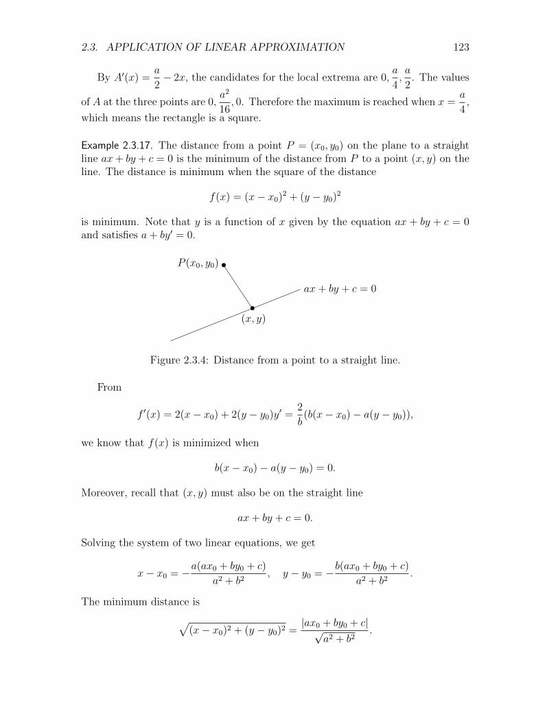
2.3. APPLICATION OF LINEAR APPROXIMATION 123
By A′(x) =a
2− 2x, the candidates for the local extrema are 0,
a
4,a
2. The values
of A at the three points are 0,a2
16, 0. Therefore the maximum is reached when x =
a
4,
which means the rectangle is a square.
Example 2.3.17. The distance from a point P = (x0, y0) on the plane to a straightline ax+ by + c = 0 is the minimum of the distance from P to a point (x, y) on theline. The distance is minimum when the square of the distance
f(x) = (x− x0)2 + (y − y0)2
is minimum. Note that y is a function of x given by the equation ax + by + c = 0and satisfies a+ by′ = 0.
ax+ by + c = 0
P (x0, y0)
(x, y)
Figure 2.3.4: Distance from a point to a straight line.
From
f ′(x) = 2(x− x0) + 2(y − y0)y′ =2
b(b(x− x0)− a(y − y0)),
we know that f(x) is minimized when
b(x− x0)− a(y − y0) = 0.
Moreover, recall that (x, y) must also be on the straight line
ax+ by + c = 0.
Solving the system of two linear equations, we get
x− x0 = −a(ax0 + by0 + c)
a2 + b2, y − y0 = −b(ax0 + by0 + c)
a2 + b2.
The minimum distance is√(x− x0)2 + (y − y0)2 =
|ax0 + by0 + c|√a2 + b2
.

124 CHAPTER 2. DIFFERENTIATION
lL
x
y
speed u
speedv
P
a
A
Q
b
B
Figure 2.3.5: Snell’s law.
Example 2.3.18. Consider light traveling from a point A in one medium to point Bin another medium. Fermat’s principle says that the path taken by the light is thepath of shortest traveling time.
Let u and v be the speed of light in the respective medium. Let L be the placewhere two media meet. Draw lines AP and BQ perpendicular to L. Let the lengthof AP,BP, PQ be a, b, l. Let x be the angle by which the light from A hits L. Lety be the angle by which the light leaves L and reaches B.
The angles x and y are related by
a tanx+ b tan y = l.
This can be considered as an equation that implicitly defines y as a function of x.The derivative of y = y(x) can be obtained by implicit differentiation
y′(x) = −a sec2 x
b sec2 y.
The time it takes for the light to travel from A to B is
T =a secx
u+b sec y
v.
By thinking of y as a function of x, the time T becomes a function of x. The timewill be shortest when
0 =dT
dx=a secx tanx
u+b sec y tan y
vy′
=a secx tanx
u− b sec y tan y
v
a sec2 x
b sec2 y
= a sec2 x
(sinx
u− sin y
v
).
This means that the ratio between the sine of the angles x and y is the same as theratio between the speeds of light
sinx
sin y=u
v.

2.4. MEAN VALUE THEOREM 125
This is Snell’s law of refraction.
Exercise 2.3.20. A rectangle is inscribed in an isosceles triangle. Show that the biggestarea possible is half of the area of the triangle.
Exercise 2.3.21. Among all the rectangles with area A, which one has the smallest perime-ter?
Exercise 2.3.22. Among all the rectangles with perimeter L, which one has the biggestarea?
Exercise 2.3.23. A rectangle is inscribed in a circle of radius R. When does the rectanglehave the biggest area?
Exercise 2.3.24. Determine the dimensions of the biggest rectangle inscribed in the ellipsex2
a2+y2
b2= 1.
Exercise 2.3.25. Find the volume of the biggest right circular cone with a given slant heightl.
Exercise 2.3.26. What is the shortest distance from the point (2, 1) to the parabola y =2x2?
2.4 Mean Value Theorem
If one travels between two cities at the average speed of 100 kilometers per hour,then we expect that the speed reaches exactly 100 kilometers per hour somewhereduring the trip. Mathematically, let f(t) be the distance traveled by the time t.Then the average speed from the time a to time b is
f(b)− f(a)
b− a.
Our expectation can be interpreted as
f(b)− f(a)
b− a= f ′(c) for some c ∈ (a, b).
2.4.1 Mean Value Theorem
Theorem 2.4.1 (Mean Value Theorem). If f(x) is continuous on [a, b] and differen-tiable on (a, b), then there is c ∈ (a, b), such that
f(b)− f(a)
b− a= f ′(c).

126 CHAPTER 2. DIFFERENTIATION
The conclusion can also be expressed as
f(b)− f(a) = f ′(c)(b− a), for some a < c < b,
orf(a+ h)− f(a) = f ′(a+ θh)h, for some 0 < θ < 1.
We also note that the conclusion is symmetric in a, b. Therefore there is no need toinsist a < b.
a c c c b
f(a)
f(b)
L(x)
f(x)
Figure 2.4.1: Mean value theorem.
Geometrically, the Mean Value Theorem means that the straight line L connect-ing the two ends (a, f(a)) and (b, f(b)) of the graph of f is parallel to the tangentof the function somewhere. Figure 2.4.1 suggests that c in the Mean Value Theo-rem is the place where the the distance between the graphs of f and L has localextrema. Since such local extrema for the distance f(x) − L(x) always exists byTheorem 2.3.1, we get (f − L)′(c) = 0 for some c by Theorem 2.3.4. Therefore
f ′(c) = L′(c) =f(b)− f(a)
b− a.
Example 2.4.1. We try to verify the Mean Value Theorem for f(x) = x3− 3x+ 1 on[−1, 1]. This means finding c, such that
f ′(c) = 3(c2 − 1) =f(1)− f(−1)
1− (−1)=−1− 3
1− (−1)= −2.
We get c = ± 1√3
.
Example 2.4.2. By the Mean Value Theorem, we have
log(1 + x) = log(1 + x)− log 1 =1
1 + θxx for some 0 < θ < 1.
Sincex
1 + x≤ 1
1 + θxx ≤ x for x > −1,

2.4. MEAN VALUE THEOREM 127
we conclude thatx
1 + x≤ log(1 + x) ≤ x.
The inequality already appeared in Example 2.3.9.
Example 2.4.3. For the function |x| on [−1, 1], there is no c ∈ (−1, 1) satisfying
f(1)− f(−1) = 0 = f ′(c)(1− (−1)).
The Mean Value Theorem does not apply because |x| is not differentiable at 0.
Exercise 2.4.1. Is the conclusion of the Mean Value Theorem true? If true, find c. If not,explain why.
1. x3 on [−1, 1].
2. 2x on [0, 1].
3.1
xon [1, 2].
4. |x3−3x+1| on [−1, 1].
5.√|x| on [−1, 1].
6. cosx on [−a, a].
7. log x on [1, 2].
8. log |x| on [−1, 1].
9. arcsinx on [0, 1].
Exercise 2.4.2. Suppose f(1) = 2 and f ′(x) ≤ 3 on R. How large and how small can f(4)be? What happens when the largest or the smallest value is reached? How about f(−4)?
Exercise 2.4.3. Prove inequality.
1. | sinx− sin y| ≤ |x− y|.
2.x− yx
< logx
y<x− yy
, for x > y > 0.
3. | arctanx− arctan y| ≤ |x− y|.
Exercise 2.4.4. Find the biggest interval on which |ex−ey| > |x−y|? What about |ex−ey| <|x− y|?
Exercise 2.4.5. Suppose f(x) is continuous at x0 and differentiable on (x0−δ, x0)∪(x0, x0+δ). Prove that if limx→x0 f
′(x) = l converges, then f(x) is differentiable at x0 and f ′(x0) =l.
2.4.2 Criterion for Constant Function
The Mean Value Theorem can be used to prove Theorem 2.3.2: If f ′ ≥ 0 on aninterval, then for any x1 < x2 on the interval, by the Mean Value Theorem, we have
f(x2)− f(x1) = f ′(c)(x2 − x1) ≥ 0.
For the special case f ′ = 0 throughout the interval, the argument gives the followingresult.

128 CHAPTER 2. DIFFERENTIATION
Theorem 2.4.2. If f ′(x) = 0 for all x ∈ (a, b), then f(x) is a constant on (a, b).
Applying the theorem to f(x)− g(x), we get the following result.
Theorem 2.4.3. If f ′(x) = g′(x) for all x ∈ (a, b), then there is a constant C, suchthat f(x) = g(x) + C on (a, b).
Example 2.4.4. The function ex satisfies f(x)′ = f(x). Are there any other functionssatisfying the equation?
If f(x)′ = f(x). Then
(e−xf(x))′ = (e−x)′f(x) + e−x(f(x))′ = ex(−f(x) + f ′(x)) = 0.
Therefore e−xf(x) = C is a constant, and f(x) = Cex.
Example 2.4.5. Suppose f ′(x) = x and f(1) = 2. Then f ′(x) =
(x2
2
)′implies
f(x) =x2
2+C for some constant C. By taking x = 1, we get 2 =
1
2+C. Therefore
C =3
2and f(x) =
x2 + 3
2.
Example 2.4.6. By
(arcsinx)′ =1√
1− x2, (arccosx)′ = − 1√
1− x2.
we have (arcsin x+arccos x)′ = 0, and we have arcsinx+arccos x = C. The constantcan be determined by taking a special value x = 0
C = arcsin 0 + arccos 0 = 0 +π
2=π
2.
Therefore we havearcsinx+ arccosx =
π
2.
Exercise 2.4.6. Prove that a differentiable function is linear on an interval if and only if itsderivative is a constant.
Exercise 2.4.7. Find all functions on an interval satisfying the following equations.
1. f ′(x) = −2f(x).
2. f ′(x) = xf(x).
3. f ′(x) = f(x)2
4. f ′(x)f(x) = 1.
Exercise 2.4.8. Prove equality.

2.4. MEAN VALUE THEOREM 129
1. arctanx+ arctanx−1 =π
2, for x 6= 0.
2. 3 arccosx− arccos(3x− 4x3) = π, for |x| ≤ 1
2.
3. arctanx+ a
1− ax− arctanx = arctan a, for ax < 1.
4. arctanx+ a
1− ax− arctanx = arctan a− π, for ax > 1.
2.4.3 L’Hospital’s Rule
The following limits cannot be computed by simple arithmetic rules.
0
0: limx→1
x3 − 1
x− 1, limx→0
sinx
x, limx→0
log(1 + x)
x;
∞∞
: limx→0
log x
x−1, limx→∞
log x
x, limx→∞
x2
ex;
1∞ : limx→∞
(1 +
1
x
)x, limx→0
(1 + sin x)log x;
∞−∞ : limx→0
(1
x− 1
ex − 1
).
We say these limits are indeterminate. Other indeterminates include 0 ·∞, ∞+∞,00, ∞0. The derivative can help us computing such limits.
Theorem 2.4.4 (L’Hospital’s Rule). Suppose f(x) and g(x) are differentiable func-tions on (a, b), with g′(x) 6= 0. Suppose
1. Either limx→a+ f(x) = limx→a+ g(x) = 0 or limx→a+ f(x) = limx→a+ g(x) =∞.
2. limx→a+
f ′(x)
g′(x)= l converges.
Then limx→a+
f(x)
g(x)= l.
The theorem computes the limits of the indeterminates of type0
0or∞∞
. The
conclusion is the equality
limx→a+
f(x)
g(x)= lim
x→a+
f ′(x)
g′(x)
whenever the right side converges. It is possible that the left side converges but theright side diverges.

130 CHAPTER 2. DIFFERENTIATION
The theorem also has a similar left sided version, and the left and right sidedversions may be combined to give the two sided version. Moreover, l’Hospital’s rulealso allows a or l to be any kind of infinity.
The reason behind l’Hospital’s rule is the following version of the Mean ValueTheorem, which can be proved similar to the Mean Value Theorem.
Theorem 2.4.5 (Cauchy’s Mean Value Theorem). If f(x) and g(x) are continuouson [a, b] and differentiable on (a, b), such that g′(x) 6= 0 on (a, b), then there isc ∈ (a, b), such that
f(b)− f(a)
g(b)− g(a)=f ′(c)
g′(c).
Consider the parametrized curve (g(t), f(t)) for t ∈ [a, b]. The theorem says thatthe straight line connecting the two ends (g(a), f(a)) and (g(b), f(b)) of the curve is
parallel to the tangent of the curve somewhere. The slope of the tangent isf ′(c)
g′(c).
(g(a), f(a))
(g(b), f(b))
f ′(c)
g′(c)
Figure 2.4.2: Cauchy’s Mean Value Theorem.
For the case limx→a+ f(x) = limx→a+ g(x) = 0 of l’Hospital’s rule, we may extendf and g to continuous functions on [a, b) by assigning f(a) = g(a) = 0. Then forany a < x < b, we may apply Cauchy’s Mean Value Theorem to the functions on[a, x] and get
f(x)
g(x)=f(x)− f(a)
g(x)− g(a)=f ′(c)
g′(c)for some c ∈ (a, x).
Since x→ a+ implies c→ a+, we conclude that limc→a+
f ′(c)
g′(c)= l implies limx→a+
f(x)
g(x)=
l.
By changing the variable x to1
x, it is not difficult to extend the proof to the case
a = ±∞. The proof for the∞∞
type is must more complicated and is omitted here.
Example 2.4.7. In Example 1.2.15, we proved that limx→+∞ ax = 0 for 0 < a < 1.
Exercise 1.6.15 extended the limit to limx→+∞ x2ax = 0. We derive the second limit
from the first one by using l’Hospital’s rule.
2.4. MEAN VALUE THEOREM 131
We have b =1
a> 1, and limx→+∞ a
x = 0 is the same as limx→+∞ bx = ∞. We
also have limx→+∞ x2 = ∞. Therefore limx→+∞ x
2ax = limx→+∞x2
bxis of type
∞∞
,
and we may apply l’Hospital’s rule (twice)
limx→+∞
x2
bx=(3) lim
x→+∞
(x2)′
(bx)′= lim
x→+∞
2x
bx log b
=(2) limx→+∞
(2x)′
(bx log b)′= lim
x→+∞
2
bx(log b)2=(1) 0.
Here is the precise reason behind the computation. The equality =(1) is fromExample 1.2.15. Then by l’Hospital’s rule, the convergence of the right side of =(2)
implies the convergence of the left side of =(2) and the equality =(2) itself. The left of=(2) is the same as the right side of =(3). By l’Hospital’s rule gain, the convergence ofthe right side of =(3) implies the convergence of the left side of =(3) and the equality=(3).
Example 2.4.8. Applying l’Hospital’s rule to the limit limx→0sinx
xof type
0
0, we get
limx→0
sinx
x= lim
x→0
(sinx)′
(x)′= lim
x→0cosx = 1.
However, this argument is logically circular because it makes use of the formula(sinx)′ = cosx. A special case of this formula is
limx→0
sinx
x= (sinx)′|x=0 = 1,
which is exactly the conclusion we try to get.
Exercise 2.4.9. Are the application of l’Hospital’s rule logically circular?
1. limx→0x
sinx.
2. limx→0cosx− 1
x.
3. limx→0cosx− 1
x2.
4. limx→1x2 − 1
x− 1.
5. limx→1x2 − 1
x3 − 1.
6. limx→0log(1 + x)
x.
132 CHAPTER 2. DIFFERENTIATION
Example 2.4.9. By blindly using l’Hospital’s rule four times, we have
limx→0
sin2 x− sinx2
x4= lim
x→0
2 sinx cosx− 2x cosx2
4x3
= limx→0
cos2 x− sin2 x− cosx2 + 2x2 sinx2
6x2
= limx→0
−4 cosx sinx+ 6x sinx2 + 4x3 cosx2
12x
= limx→0
4 sin2 x− 4 cos2 x+ 6 sinx2 + 24x2 cosx2 − 8x4 sinx2
12
= −1
3.
We find that it is increasingly difficult to calculate the derivatives. The followingcompute the the limit after calculating the derivatives twice.
limx→0
sin2 x− sinx2
x4= lim
x→0
2 sinx cosx− 2x cosx2
4x3
= limx→0
cos2 x− sin2 x− cosx2 + 2x2 sinx2
6x2
= limx→0
(−1
3
(sinx
x
)2
+1− cosx2
6x2+
1
3sinx2
)= −1
3· 12 + 0 +
1
3· 0 = −1
3.
In fact, the smartest way is not to calculate the derivatives at all. See Example2.5.11.
Exercise 2.4.10. Use l’Hospital’s rule to compute the limits.
1. limx→0sinx− x
x3.
2. limx→0sinx− tanx
x3.
3. limx→0ex − esinx
x3.
4. limx→0cos(sinx)− cosx
x4.
5. limx→01− cosx2
x3 sinx.
6. limx→1xx − x
log x− x+ 1.
7. limx→0x− tanx
x− sinx.
8. limx→1(x− 1) log x
1 + cosπx.
Example 2.4.10. The limit limx→0+ x log x is of type 0 · ∞. We convert into type∞∞
and apply l’Hospital’s rule (in the second equality)
limx→0+
x log x = limx→0+
log x
x−1= lim
x→0+
x−1
−x−2= lim
x→0+−x = 0.
2.5. HIGH ORDER APPROXIMATION 133
The similar argument gives
limx→0+
xp log x = 0, for p > 0.
Taking a positive power of the limit, we further get
limx→0+
xp(− log x)q = 0, for p, q > 0.
By converting x to1
x, we also have
limx→+∞
(log x)q
xp= 0, for p, q > 0.
Example 2.4.11. We compute the limit in Example 2.5.13 by first converting it to
type0
0and then applying l’Hospital’s rule
limx→0
(1
x− 1
ex − 1
)= lim
x→0
ex − 1− xx(ex − 1)
= limx→0
ex − 1
ex − 1 + xex= lim
x→0
ex
2ex + xex=
1
2.
Example 2.4.12. If we apply l’Hospital’s rule to the limit limx→∞x+ sinx
xof type
∞∞
, then we get
limx→∞
x+ sinx
x= lim
x→∞(1 + cos x).
We find that the left converges and the right diverges. The reason for the l’Hospital’srule to fail is that the second condition is not satisfied.
2.5 High Order Approximation
Linear approximations can be used to solve many problems. When linear approxi-mations are not enough, however, we may use high order approximations.
Definition 2.5.1. An n-th order approximation of f(x) at x0 is a degree n polynomial
P (x) = a0 + a1(x− x0) + a2(x− x0)2 + · · ·+ an(x− x0)n,
such that for any ε > 0, there is δ > 0, such that
|x− x0| < δ =⇒ |f(x)− P (x)| ≤ ε|x− x0|n.
A function is n-th order differentiable if it has n-order approximation.

134 CHAPTER 2. DIFFERENTIATION
The error Rn(x) = f(x) − P (x) of the approximation is called the remainder.The definition means that
f(x) = P (x) +Rn(x)
= a0 + a1(x− x0) + a2(x− x0)2 + · · ·+ an(x− x0)n + o((x− x0)n),
where the “small o” notation means that the remainder term satisfies
limx→a
f(x)− P (x)
(x− x0)n= lim
x→a
Rn(x)
(x− x0)n= 0.
The n-th order approximation of a function is unique. See Exercise 2.5.7. More-over, if m < n, then the truncation a0 + a1(x−x0) + a2(x−x0)2 + · · ·+ am(x−x0)m
is the m-th order approximation of f at x0. After all, if we have the 10th orderapproximation, then we should also have the 5th order approximation.
Example 2.5.1. We have
x4 = (1 + (x− 1))4 = 1 + 4(x− 1) + 6(x− 1)2 + 4(x− 1)3 + (x− 1)4.
For any ε > 0, we have |x− 1| < δ = min{
1,ε
5
}implying
|x4 − 1− 4(x− 1)− 6(x− 1)2| = |4(x− 1)3 + (x− 1)4| ≤ (4 + |x− 1|)|x− 1|3
≤ (4 + 1)ε
5|x− 1|2 = ε|x− 1|2.
Therefore 1 + 4(x − 1) + 6(x − 1)2 is the quadratic approximation of x4 at 1. Bysimilar argument, we get approximations of other orders.
linear : 1 + 4(x− 1),
quadratic : 1 + 4(x− 1) + 6(x− 1)2,
cubic : 1 + 4(x− 1) + 6(x− 1)2 + 4(x− 1)3,
quartic : 1 + 4(x− 1) + 6(x− 1)2 + 4(x− 1)3 + (x− 1)4,
quintic : 1 + 4(x− 1) + 6(x− 1)2 + 4(x− 1)3 + (x− 1)4,
...
Example 2.5.2. The limit
limx→0
cosx− 1
x2= −1
2in Example 1.5.18 can be interpreted as
limx→0
cosx− 1 +1
2x2
x2= 0.
This means that cosx is second order differentiable at 0, with quadratic approxima-
tion 1− 1
2x2.

2.5. HIGH ORDER APPROXIMATION 135
Exercise 2.5.1. Prove that1
1− x= 1 + x+ x2 + · · ·+ xn +
xn+1
1− x. What does this tell you
about the differentiability of1
1− xat 0?
Exercise 2.5.2. Show that1
1 + xand
1
1 + x2are differentiable of arbitrary order. What
are their high order approximations?
Exercise 2.5.3. What is the n-th order approximation of 1 + 2x+ 3x2 + · · ·+ 100x100 at 0?
Exercise 2.5.4. Use l’Hospital’s rule to compute the limits. Then interpret your results ashigh order approximations.
1. limx→0sinx− x
x3.
2. limx→0sinx2 − x2
x6.
3. limx→0sin2 x− x2
x4.
4. limx→01
x5
(sinx− x+
1
6x3
).
5. limx→0sinx− tanx
x3.
6. limx→01
x3
(ex − 1− x− 1
2x2
).
7. limx→01
x3
(log(1 + x)− x+
1
2x2
).
8. limx→12 log x+ (x− 1)(x− 3)
(x− 1)3.
Exercise 2.5.5. For what choice of a, b, c is the function{x4, if x ≥ 1,
a+ bx+ cx2, if x < 1,
second order differentiable at 1? Is it possible for the function to be third order differen-tiable?
Exercise 2.5.6. Suppose f(x) is second order differentiable at 0. Show that
3f(x)− 3f(2x) + f(3x) = f(0) + o(x2).
Exercise 2.5.7. Suppose P (x) = a0 + a1(x− a) + a2(x− a)2 satisfies limx→aP (x)
(x− a)2= 0.
Prove that a0 = a1 = a2 = 0. Then explain that the result means the uniqueness ofquadratic approximation. Moreover, extend the result to high order approximation.
Exercise 2.5.8. Suppose P (x) is the n-order approximation of f(x). What is the n-orderapproximation of f(−x)? Then use Exercise 2.5.7 to explain that the high order ap-proximation of an even function has not odd power terms. What about the high orderapproximation of an odd function?

136 CHAPTER 2. DIFFERENTIATION
2.5.1 Taylor Expansion
The linear approximation may be computed by the derivative. The high orderapproximation may be computed by repeatedly taking the derivative. The idea issuggested by the following example. By applying l’Hospital’s rule three times, weget a more precise limit than the one in Example 2.5.2
limx→0
cosx− 1 +1
2x2
x3= lim
x→0
− sinx− x3x2
= limx→0
− cosx− 1
3 · 2x= lim
x→0
sinx
3 · 2 · 1= 0.
Each application of the l’Hospital’s rule means taking derivative once. Therefore weget the third order approximation of cos x at 0 by taking derivative three times.
If f(x) is differentiable everywhere on an open interval, then the derivative f ′(x)is a function on the open interval. If the derivative function f ′(x) is also differ-entiable, then we get the second order derivative f ′′(x) = (f ′(x))′. If the functionf ′′(x) is yet again differentiable, then taking the derivative one more time gives thethird order derivative f ′′′(x) = (f ′′(x))′. The process may continue and we havethe n-th order derivative f (n)(x). The Leibniz notation for the high order derivative
f (n)(x) isdnf
dxn.
Let f(x) = cos x and P (x) = 1 − 1
2x2. The key to the repeated application of
the l’Hospital’s rule is that the numerator is always 0 at x0 = 0. This means that
f(x0) = P (x0), f ′(x0) = P ′(x0), f ′′(x0) = P ′′(x0), f ′′′(x0) = P ′′′(x0).
In general, if P (x) = a0 + a1(x − x0) + a2(x − x0)2 + a3(x − x0)3, then the aboveequalities become
f(x0) = a0, f′(x0) = a1, f
′′(x0) = 2a2, f′′′(x0) = 3 · 2a3.
Theorem 2.5.2. If f(x) has n-th order derivative at x0, then f is n-th order differ-entiable, with n-th order approximation
Tn(x) = f(x0) + f ′(x0)(x− x0) +f ′′(x0)
2!(x− x0)2 + · · ·+ f (n)(x0)
n!(x− x0)n.
The polynomial Tn is called the n-th order Taylor expansion of f .Note that the existence of the derivative f (n)(x0) implicitly assumes that f (k)(x)
exists for all x near x0 and all k < n. The theorem gives one way (but not the onlyway!) to compute the high order approximation in case the function has high orderderivative. However, we will show in Example 2.5.8 that it is possible to have highorder approximation without the existence of the high order derivative. Here theconcept (high order differentiability) is strictly weaker than the computation (highorder derivative).

2.5. HIGH ORDER APPROXIMATION 137
Example 2.5.3. The high order derivatives of the power function xp are
(xp)′ = pxp−1,
(xp)′′ = p(p− 1)xp−2,
...
(xp)(n) = p(p− 1) · · · (p− n+ 1)xp−n.
More generally, we have
((a+ bx)p)(n) = p(p− 1) · · · (p− n+ 1)bn(a+ bx)p−n.
For a = b = 1, we get the Taylor expansion at 0
(1 + x)p = 1 + px+p(p− 1)
2!x2 + · · ·+ p(p− 1) · · · (p− n+ 1)
n!xn + o(xn).
For a = 1, b = −1 and p = −1, we get the Taylor expansion at 0
1
1− x= 1 + x+ x2 + · · ·+ xn + o(xn).
You may compare with Exercise 2.5.1.
Example 2.5.4. By (log x)′ = x−1 and the derivatives from Example 2.5.3, we have
(log x)(n) = (−1)n−1 (n− 1)!
xn. This gives the Taylor expansion at 1
log x = (x− 1)− 1
2(x− 1)2 +
1
3(x− 1)3 − · · ·+ (−1)n+1 1
n(x− 1)n + o((x− 1)n).
This can also be expressed as a Taylor expansion at 0
log(1 + x) = x− 1
2x2 +
1
3x3 − · · ·+ (−1)n+1 1
nxn + o(xn).
Example 2.5.5. By (ex)′ = ex, it is easy to see that (ex)(n) = ex for all n. This givesthe Taylor expansion at 0
ex = 1 +1
1!x+
1
2!x2 + · · ·+ 1
n!xn + o(xn).
Example 2.5.6. The high order derivatives of sin x and cos x are 4-periodic in thesense that sin(n+4) x = sin(n) x and cos(n+4) x = cos(n) x, and are given by
(sinx)′ = cosx, (cosx)′ = − sinx,
(sinx)′′ = − sinx, (cosx)′′ = − cosx,
(sinx)′′′ = − cosx, (cosx)′′′ = sinx,
(sinx)′′′′ = sinx, (cosx)′′′′ = cosx.

138 CHAPTER 2. DIFFERENTIATION
This gives the Taylor expansions at 0
sinx = x− 1
3!x3 +
1
5!x5 − · · ·+ (−1)n+1 1
(2n− 1)!x2n−1 + o(x2n),
cosx = 1− 1
2!x2 +
1
4!x4 − · · ·+ (−1)n
1
(2n)!x2n + o(x2n+1).
Note that we have o(x2n) for sinx at the end, which is more accurate than o(x2n−1).The reason is that the 2n-th term 0 · x2n is omitted from the expression, so that theapproximation is actually of 2n-th order. The similar remark applies to cosx.
We also note that the Taylor expansions of ex, sinx, cosx are related by theequality
eix = cosx+ i sinx, i =√−1.
Exercise 2.5.9. Prove the following properties of high order derivative
(f + g)(n) = f (n) + g(n),
(cf)(n) = cf (n),
(fg)(n) =n∑i=0
n!
i!(n− i)!f (i)g(j).
Exercise 2.5.10. Prove the chain rule for second order derivative
(g(f(x)))′′ = g′′(f(x))f ′(x)2 + g′(f(x))f ′′(x).
Exercise 2.5.11. Compute derivatives of all order.
1. ax.
2. eax+b.
3. sin(ax+ b).
4. cos(ax+ b).
5. log(ax+ b).
6. logax+ b
cx+ d.
7.ax+ b
cx+ d.
8.1
(ax+ b)(cx+ d).
Exercise 2.5.12. Compute high order derivatives.
1. (tanx)′′′.
2. (secx)′′′.
3. (sinx2)′′′.
4. (arcsinx)′′.
5. (arctanx)′′.
6. (xx)′′.
7.d2
dx2
(1 +
1
x
)x.
Exercise 2.5.13. Use high order derivatives to find high order approximations.
1. ax, n = 5, at 0.
2. ax, n = 5, at 1.
3. sin2 x, n = 6, at 0.
4. sin2 x, n = 6, at π.
5. ex2, n = 6, at 0.
6. ex2, n = 6, at 1.
7. x3ex, n = 5, at 0.
8. x3ex, n = 5, at 1.
9. ex sinx, n = 5 at 1.

2.5. HIGH ORDER APPROXIMATION 139
Exercise 2.5.14. Compute high order derivatives.
1. (x2 + 1)ex. 2. (x2 + 1) sinx. 3. x2(x− 1)p. 4. x log x.
Exercise 2.5.15. Prove (xn−1e1x )(n) =
(−1)n
xn+1e
1x .
Exercise 2.5.16. Prove (eax sin(bx+ c))(n) = (a2 + b2)n2 eax sin(bx+ c+ nθ), where sin θ =
b√a2 + b2
. What is the similar formula for (eax cos(bx+ c))(n)?
Exercise 2.5.17. Suppose f(x) has second order derivative near x0. Prove that
f ′′(x0) = limh→0
f(x0 + h) + f(x0 − h)− 2f(x0)
h2.
Exercise 2.5.18. Compare ex, sinx, cosx, log(1 + x) with their Taylor expansions. For ex-
ample, is ex bigger than or smaller than 1 + x+x2
2!+x3
3!+ · · ·+ xn
n!?
2.5.2 High Order Approximation by Substitution
The functions (and their variations) in Examples 2.5.3 through 2.5.11 are the onlyones that we can compute all the high order derivative functions. These give the ba-sic examples of high order approximations. We get other high order approximationsby combining the basic ones.
Example 2.5.7. Substituting x byb
ax in the Taylor expansion of (1 + x)p, we get
(a+ bx)p = ap(
1 +b
ax
)p= ap
[1 + p
b
ax+
p(p− 1)
2!
b2
a2x2 + · · ·
+p(p− 1) · · · (p− n+ 1)
n!
bn
anxn + o
(bn
anxn)]
= ap + pap−1bx+p(p− 1)
2!ap−2b2x2 + · · ·
+p(p− 1) · · · (p− n+ 1)
n!ap−nbnxn + o(xn).
Note that we used apo
(bn
anxn)
= o(xn) in the computation. The reason is that
o
(bn
anxn)
really means a function R
(bn
anxn)
, where R(x) is the remainder of the

140 CHAPTER 2. DIFFERENTIATION
n-th order Taylor expansion of (1 + x)p. Since limx→0R(x)
xn= 0, we get
limx→0
apR
(bn
anxn)
xn= lim
y→0
apR(y)an
bnyn
= ap−nbn limy→0
R(y)
yn= 0.
This means apR
(bn
anxn)
= o(xn).
Further substitution of a, b, x by x0, 1, x− x0 gives the Taylor expansion of xp atx0
xp = (x0 + (x− x0))p
= xp0 + pxp−10 (x− x0) +
p(p− 1)
2!xp−2
0 (x− x0)2 + · · ·
+p(p− 1) · · · (p− n+ 1)
n!xp−n0 (x− x0)n + o((x− x0)n).
The Taylor expansion can also be obtained from the high order derivative in Example2.5.3.
Example 2.5.8. The Taylor expansion of1
1− xat 0 in Example 2.5.3 induces the
following approximations
1
1 + x= 1− x+ x2 − · · ·+ (−1)nxn + o(xn),
1
1 + x2= 1− x2 + x4 − · · ·+ (−1)nx2n + o(x2n).
Similar to the Taylor expansions of sinx and cosx, we expect that the odd power
terms vanish in the Taylor expansion of1
1 + x2. Therefore the remainder should be
improved to o(x2n+1). To get the improved remainder, we consider the 2(n + 1)-th
order Taylor expansion of1
1 + x2
1
1 + x2= 1− x2 + x4 − · · ·+ (−1)nx2n + (−1)n+1x2(n+1) + o(x2(n+1)).
This shows that the remainder of the 2n-th order Taylor expansion is (−1)n+1x2(n+1)+
R(x), where R(x) satisfies limx→0R(x)
x2(n+1)= 0. By
limx→0
(−1)n+1x2(n+1) +R(x)
x2n+1= 0 = lim
x→0
((−1)n+1x+
R(x)
x2(n+1)x
)= 0,

2.5. HIGH ORDER APPROXIMATION 141
we get
(−1)n+1x2(n+1) + o(x2(n+1)) = o(x2n+1),
and the improved approximation
1
1 + x2= 1− x2 + x4 − · · ·+ (−1)nx2n + o(x2n+1).
Finally, it is easy to see that1
1 + x2has derivative of any order. From the
coefficients in the Taylor expansion, we get
dn
dxn
∣∣∣∣x=0
(1
1 + x2
)= n!an =
{0, if n = 2k − 1,
(−1)k(2k)!, if n = 2k.
It is practically impossible to get this by directly computing the high order deriva-tives (i.e., by repeatedly taking derivatives).
Exercise 2.5.19. Explain and justify the following claims about remainders.
1. o(x5) = o(x3).
2. o(x5) + o(x5) = o(x5).
3. o(x4) + o(x5) = o(x3).
4. x3o(x5) = o(x8).
5. o(x3)o(x5) = o(x8).
6. o(x3) + x5 = o(x3).
Exercise 2.5.20. Find the Taylor expansion of1
1− x3at 0, and the high order derivatives
of the function at 0.
Exercise 2.5.21. Use the high order derivatives in Example 2.5.8 to find the Taylor expan-sion of arctanx at 0.
Exercise 2.5.22. Find the Taylor expansion of1√
1− x2at 0. Find the high order derivatives
of the function at 0. Then find the Taylor expansion of arcsinx at 0.
Example 2.5.9. The Taylor expansion of ex at 0 induces
e−x = 1− 1
1!x+
1
2!x2 − · · ·+ (−1)n
1
n!xn + o(xn),
ex = ex0ex−x0 = ex0 − 1
1!ex0(x− x0) +
1
2!ex0(x− x0)2 − · · ·
+ (−1)n1
n!ex0(x− x0)n + o((x− x0)n),
ex2
= 1 +1
1!x2 +
1
2!x4 + · · ·+ 1
n!x2n + o(x2n+1).

142 CHAPTER 2. DIFFERENTIATION
Note that we have the more accurate remainder o(x2n+1) for ex2
for the reason similarto Example 2.5.8. Moreover, the Taylor expansion of ex
2gives
(ex2
)(n)|x=0 =
0, if n = 2k − 1,(2k)!
k!, if n = 2k.
Example 2.5.10. The high order approximation of x2ex at 0 is
x2ex = x2
(1 +
1
1!x+
1
2!x2 + · · ·+ 1
n!xn + o(xn)
)= x2 +
1
1!x3 +
1
2!x4 + · · ·+ 1
n!xn+2 + o(xn+2).
Here we use x2o(xn) = o(xn+2). The n-th order approximation is
x2ex = x2 +1
1!x3 +
1
2!x4 + · · ·+ 1
(n− 2)!xn + o(xn).
Can you find the n-th order derivative of x2ex at 0?
On the other hand, to find the high order approximation of x2ex at 1, we express

2.5. HIGH ORDER APPROXIMATION 143
the variables in terms of x− 1 and get
x2ex = ((x− 1) + 1)2e(x−1)+1 = e((x− 1)2 + 2(x− 1) + 1)ex−1
= e((x− 1)2 + 2(x− 1) + 1)
(n∑i=0
1
i!(x− 1)i + o((x− 1)n)
)
= e
n∑i=0
1
i!(x− 1)i+2 + o((x− 1)n+2)
+ 2en∑i=0
1
i!(x− 1)i+1 + o((x− 1)n+1)
+ en∑i=0
1
i!(x− 1)i + o((x− 1)n)
= en∑i=2
1
(i− 2)!(x− 1)i + o((x− 1)n)
+ 2e(x− 1) + 2en∑i=2
1
(i− 1)!(x− 1)i + o((x− 1)n)
+ e+ e(x− 1) + en∑i=2
1
i!(x− 1)i + o((x− 1)n)
= e+ 3e(x− 1) + en∑i=2
(1
(i− 2)!+
2
(i− 1)!+
1
i!
)(x− 1)i + o((x− 1)n)
= e+ 3e(x− 1) + en∑i=2
i2 + i+ 1
i!(x− 1)i + o((x− 1)n).
Exercise 2.5.23. Use the basic Taylor expansions to find the high order approximationsand derivatives of functions in Exercise 2.5.11.
Exercise 2.5.24. Use the basic Taylor expansions to find the high order approximationsand derivatives at 0.
1.1
x(x+ 1)(x+ 2).
2.√
1− x2.
3.√
1 + x3.
4. log(1 + x2).
5. log(1 + 3x+ 2x2).
6. log1 + x2
1− x3.
7. e2x.
8. ax2.
9. sinx cos 2x.
10. sinx cos 2x sin 3x.
11. sinx2.
12. sin2 x.
Exercise 2.5.25. Use the basic Taylor expansions to find high order approximations andhigh order derivatives.

144 CHAPTER 2. DIFFERENTIATION
1. x3 + 5x− 1 at 1.
2. xp at −3.
3.x+ 3
x+ 1at 1.
4.√x+ 1 at 1.
5. e−2x at 4.
6. log x at 2.
7. log(3− x) at 2.
8. sinx atπ
2.
9. sinx at π.
10. cosx at π.
11. sin 2x atπ
4.
12. sin2 x at π.
Exercise 2.5.26. Use the basic Taylor expansions to find high order approximations andhigh order derivatives at x0.
1. ax.
2. x2ex.
3. log x.
4. sinx.
5. sinx cos 2x.
6. sin2 x.
2.5.3 Combination of High Order Approximations
So far we only used simple substitutions to get new approximations. In the subse-quent examples, we compute more sophisticated combinations of approximations.
Example 2.5.11. By the Taylor expansion of sinx, we have
sin2 x− sinx2 =
(x− 1
6x3 +
1
120x5 + o(x6)
)2
−(x2 − 1
6x6 + o((x2)4)
)=
(x2 − 1
3x4 +
1
36x6 +
1
60x6 + o(x6)2 + 2xo(x6) + · · ·
)−(x2 − 1
6x6 + o(x8)
)= −1
3x4 +
19
90x6 + o(x7).
The term o(x7) at the end comes from
limx→0
R(x)
x6= 0 =⇒ lim
x→0
R(x)2
x7= 0, lim
x→0
xR(x)
x7= 0, . . . .
In particular, we get the limit in Example 2.4.9
limx→0
sin2 x− sinx2
x4= −1
3.
We also get the high order derivatives of f(x) = sin2 x− sinx2 at 0
f ′(0) = f ′′(0) = f ′′′(0) = f (5)(0) = 0, f (4)(0) = −8, f (6)(0) = 152.

2.5. HIGH ORDER APPROXIMATION 145
Example 2.5.12. We may compute the Taylor expansions of tanx and secx from the
Taylor expansions of sinx, cos x and1
1− x
secx =1
cosx=
1
1− 1
2x2 +
1
24x4 + o(x5)
= 1 +
(1
2x2 − 1
24x4 + o(x5)
)+
(1
2x2 − 1
24x4 + o(x5)
)2
+
(1
2x2 − 1
24x4 + o(x5)
)3
+ o(x6)
= 1 +1
2x2 − 1
24x4 +
1
4x4 + o(x5)
= 1 +1
2x2 +
5
24x4 + o(x5),
tanx = sinx secx =
(x− 1
6x3 +
1
120x5 + o(x6)
)(1 +
1
2x2 +
5
24x4 + o(x5)
)= x− 1
6x3 +
1
120x5 +
1
2x3 − 1
12x5 +
5
24x5 + o(x6)
= x+1
3x3 +
2
15x5 + o(x6).
The expansions give (secx)(4)x=0 = 5 and (tan x)
(5)x=0 = 16.
Example 2.5.13. We computed limx→0
(1
x− 1
ex − 1
)by using l’Hospital’s rule in
Example 2.4.11. Alternatively,, we use the Taylor expansions of ex and1
1− x
1
x− 1
ex − 1=
1
x− 1
x+x2
2+ o(x2)
=1
x
1− 1
1 +x
2+ o(x)
=
1
x
(1− 1 +
(x2
+ o(x))
+ o(x
2+ o(x)
))=
1
2+o(x)
x.
This implies that the limit is1
2.
Example 2.5.14. We know limx→∞
(1 +
1
x
)x= e from Example 1.6.17. The next
question is what the difference
(1 +
1
x
)x− e looks like. As x goes to infinity, does
the difference approach 0 like1
x?

146 CHAPTER 2. DIFFERENTIATION
The question is the same as the behavior of (1 + x)1x − e near 0. By the Taylor
expansions of log(1 + x) and ex at 0, we get
(1 + x)1x − e = e
1x
log(1+x) − e
= e1x
(x−x
2
2+o(x2)
)− e
= e(e−
x2
+o(x) − 1)
= e[(−x
2+ o(x)
)+ o
(−x
2+ o(x)
)]= −e
2x+ o(x).
Translated back into x approaching infinity, we have(1 +
1
x
)x− e = − e
2x+ o
(1
x
).
Exercise 2.5.27. Find the 5-th order approximations at 0.
1. ex sinx.
2.√x+ 1ex
2tanx.
3. (1 + x)x.
4. logsinx
x.
5. log cosx.
6.x
ex − 1.
Exercise 2.5.28. Use approximations to compute limits.
1. limx→01− cosx2
x3 sinx.
2. limx→0sinx− tanx
x3.
3. limx→0
(1
sin2 x− 1
x2
).
4. limx→0
(1
x2− 1
tan2 x
).
5. limx→1
(x
x− 1− 1
log x
).
6. limx→0(cosx+ sinx)1
x(x+1) .
7. limx→0ex − esinx
x3.
8. limx→0 logcos ax
cos bx.
9. limx→0x− tanx
x− sinx.
10. limx→∞ x2
(e− 1
x−(
1 +1
x
)x).
11. limx→∞ x2 log
(x sin
1
x
).
12. limx→1(x− 1) log x
1 + cosπx.
Exercise 2.5.29. Use whatever method you prefer to compute limits, p, q > 0.
1. limx→0+ xpe−xq.
2. limx→+∞ xpe−x
q.
3. limx→+∞ xp log x.
4. limx→1+(x− 1)p log x.
5. limx→1+(x− 1)p(log x)q.
6. limx→+∞ xpe−x
qlog x.
2.5. HIGH ORDER APPROXIMATION 147
7. limx→+∞ xp log(log x).
8. limx→+∞(log x)p(log(log x))q.
9. limx→e+(x− e)p log(log x).
Exercise 2.5.30. Use whatever method you prefer to compute limits, p, q > 0.
1. limx→0+tanp x− xp
sinp x− xp.
2. limx→0+sinp x− tanp x
xq.
3. limx→π4
tanx− cotx
4x− π.
4. limx→0a tan bx− b tan ax
a sin bx− b sin ax.
Exercise 2.5.31. Use whatever method you prefer to compute limits.
1. limx→∞ x3
(sin
1
x− 1
2sin
2
x
).
2. limx→01
x
(2
x(2 + x)− 1
ex − 1
).
3. limx→0
(1
log(1 + x)− 1
x
).
4. limx→0
(1
log(x+√
1 + x2)− 1
log(1 + x)
).
Exercise 2.5.32. Use whatever method you prefer to compute limits.
1. limx→1− log x log(1− x).
2. limx→0+xx − 1
x log x.
3. limx→0+xx − 1− x log x
x2(log x)2.
4. limx→0+x(xx) − xx2(log x)2
.
5. limx→1xlog x − 1
(log x)2.
6. limx→1xx − x
log x− x+ 1.
Exercise 2.5.33. Use whatever method you prefer to compute limits.
1. limx→0(1 + ax)b − (1 + bx)a
x2.
2. limx→0(1 + ax+ cx2)b − (1 + bx+ dx2)a
x2.
3. limx→aax − xa
x− a.
4. limx→0(a+ x)x − ax
x2.
5. limx→0+ax − asinx
x3, a > 0.
6. limx→0+log(sin ax)
log(sin bx), a, b > 0.
7. limx→0log(cos ax)
log(cos bx).
8. limx→0cos(sinx)− cosx
x4.
9. limx→0arcsin 2x− 2 arcsinx
x3.
10. limx→01− cosx2
x2 sinx2.
11. limx→π6
1− 2 sinx
cos 3x.
12. limx→1+ log x tanπx
2.
13. limx→0+ xxx−1.
14. limx→0 xsinx.
15. limx→0+(− log x)x.
148 CHAPTER 2. DIFFERENTIATION
16. limx→0
(e−1(1 + x)
1x
) 1x.
17. limx→0(x−1 arcsinx)1x2 .
18. limx→0
(2
πarccosx
) 1x
.
19. limx→0
(cosx
1 + sinx
) 1x
.
Exercise 2.5.34. In Example 2.4.2, we applied the Mean Value Theorem to get log(1+x) =x
1 + θxfor some 0 < θ < 1.
1. Find explicit formula for θ = θ(x).
2. Compute limx→0 θ by using l’Hospital’s rule.
3. Compute limx→0 θ by using high order approximation.
You may try the same for other functions such as ex − 1 = eθx. What can you say aboutlimx→0 θ in general?
Exercise 2.5.35. Show that the limits converge but cannot be computed by L’Hospital’srule.
1. limx→0
x2 sin1
xsinx
.2. limx→∞
x− sinx
x+ sinx.
Exercise 2.5.36. Find a, b so that the following hold.
1. x− (a+ b cosx) sinx = o(x4). 2. x− a sinx− b tanx = o(x4).
2.5.4 Implicit High Order Differentiation
Example 2.5.15. In Example 2.2.9, the function y = y(x) implicitly given by the unit circle
x2 + y2 = 1 has derivative y′ = −xy
. Then
y′′ = −y − xy′
y2= −
y + xx
y
y2= −x
2 + y2
y3= − 1
y3.
You may verify the result by directly computing the second order derivative of y =±√
1− x2.
Example 2.5.16. In Example 2.2.10, we computed the derivative of the function y = y(x)implicitly given by the equation 2y − 2x2 − sin y + 1 = 0 and then obtained the linear
approximation at P =
(√π
2,π
2
). We can certainly continue finding the formula for the
second order derivative of y(x) and then get the quadratic approximation at P .

2.5. HIGH ORDER APPROXIMATION 149
Alternatively, we may compute the quadratic approximation at P by postulating theapproximation to be
y =π
2+ a1∆x+ a2∆x2 + o(∆x2), ∆x = x−
√π
2.
Substituting into the equation, we get
0 = 2(π
2+ a1∆x+ a2∆x2 + o(∆x2)
)− 2
(√π
2+ ∆x
)2
− sin(π
2+ a1∆x+ a2∆x2 + o(∆x2)
)+ 1
= 2a1∆x+ 2a2∆x2 − 4
√π
2∆x− 2∆x2 + o(∆x2)− cos(a1∆x+ a2∆x2 + o(∆x2)) + 1
= 2a1∆x+ 2a2∆x2 − 2√
2π∆x− 2∆x2 +1
2(a1∆x+ a2∆x2)2 + o(∆x2)
The coefficients of ∆x and ∆x2 on the right must vanish. Therefore
2a1 − 2√
2π = 0, 2a2 − 2 +1
2a2
1 = 0.
The solution is a1 =√
2π, a2 =2− π
2, and the quadratic approximation is
y(x) =π
2+√
2π∆x+2− π
2∆x2 + o(∆x2), ∆x = x−
√π
2.
Exercise 2.5.37. Compute quadratic approximations of implicitly defined functions.
1. y2 + 3y3 + 1 = x.
2. sin y = x.
3.x2
a2+y2
b2= 1.
4.√x+√y =√a.
5. ex+y = xy.
6. x2 + 2xy − y2 − 2x = 0.
Exercise 2.5.38. Compute quadratic approximations of functions y = y(x) given by thecurves.
1. x = sin2 t, y = cos2 t.
2. x = a(t− sin t), y = a(1− cos t).
3. x = et cos 2t, y = et sin 2t.
4. x = (1 + cos t) cos t, y = (1 + cos t) sin t.

150 CHAPTER 2. DIFFERENTIATION
2.5.5 Two Theoretical Examples
Theorem 2.5.2 tells us that the existence of high order derivative implies the highorder differentiability. The following example shows that the converse is not true.
Example 2.5.17. The function x3D(x) satisfies
|x| < δ = ε =⇒ |x3D(x)− 0| ≤ |x|3 ≤ ε|x|2.
Therefore the function is second order differentiable, with 0 = 0 + 0x + 0x2 as thequadratic approximation.
On the other hand, we have (x3D(x))′|x=0 = 0 and x3D(x) is not differentiable(because not even continuous) away from 0. Therefore the second order derivativeis not defined.
Exercise 2.5.39. Show that for any n, there is a function that is n-th order differentiableat 0 but has no second order derivative at 0.
Exercise 2.5.40. The lack of high order derivatives for the function in Example 2.5.17 isdue to discontinuity away from 0. Can you find a function with the following properties?
1. f that has first order derivative everywhere on (−1, 1).
2. f has no second order derivative at 0.
3. f is second order differentiable at 0.
The next example deals with the following intuition from everyday life. Supposewe try to measure a length by more and more refined rulers. If our readings frommeter ruler, centimeter ruler, millimeter ruler, micrometer ruler, etc, are all 0, thenthe real length should be 0. Similarly, the Taylor expansion of a function at 0 is themeasurement by “xn-ruler”. The following example shows that, even if the readingsby all the “xn-ruler” are 0, the function does not have to be 0.
Example 2.5.18. The function
f(x) =
{e−
1|x| , if x 6= 0,
0, if x = 0,
has derivative
f ′(x) =
1
x2e−
1|x| , if x > 0,
− 1
x2e−
1|x| , if x < 0,
0, if x = 0.

2.6. APPLICATION OF HIGH ORDER APPROXIMATION 151
The derivative at x 6= 0 is computed by the usual chain rule, and the derivative at0 is computed directly
f ′(0) = limx→0
1
xe−
1|x| = lim
y→∞
y
e|y|= 0.
In general, it can be inductively proved that
f (n)(x) =
p
(1
x
)e−
1x , if x > 0,
(−1)np
(−1
x
)e−
1x , if x < 0,
0, if x = 0,
where p(t) is a polynomial depending only on n.The function has the special property that the derivative of any order vanishes
at 0. Therefore the function is differentiable of any order, and all the high orderapproximations are 0
f(x) = 0 + 0x+ 0x2 + · · ·+ 0xn + o(xn).
However, the function is not 0.
The example can be understood in two ways. The first is that, for some functions,even more refined ruler is needed in order to measure “beyond all orders”. Thesecond is that the function above is not “measurable by polynomials”. The functionsthat are measurable by polynomials are call analytic, and the function above is notanalytic.
Exercise 2.5.41. Directly show (i.e., without calculating the high order derivatives) thatthe function in Example 2.5.18 is differentiable of any order, with 0 as the approximationof any order.
2.6 Application of High Order Approximation
2.6.1 High Derivative Test
Theorem 2.3.4 gives the first order derivative condition for a (two sided) differen-tiable function to have local extreme. As the subsequent examples show, the theoremonly provides candidates for the local extrema. To find out whether such candidatesare indeed local extrema, high order approximations are needed.
Let us consider the first non-trivial high order approximation at x0
f(x) = f(x0) + c(x− x0)n + o((x− x0)n) = f(x0) + c(x− x0)n(1 + o(1)), c 6= 0.

152 CHAPTER 2. DIFFERENTIATION
When x is close to x0, we have 1 + o(1) > 0 and therefore f(x) > f(x0) whenc(x − x0)n > 0 and f(x) < f(x0) when c(x − x0)n < 0. Specifically, we have thefollowing signs of c(x− x0)n for various cases.
• If n is odd and c > 0, then c(x − x0)n > 0 for x > x0 and c(x − x0)n < 0 forx < x0.
• If n is odd and c < 0, then c(x − x0)n < 0 for x > x0 and c(x − x0)n > 0 forx < x0.
• If n is even and c > 0, then c(x− x0)n > 0 for x 6= x0.
• If n is even and c < 0, then c(x− x0)n < 0 for x 6= x0.
The sign of c(x−x0)n then further determines whether f(x) < f(x0) or f(x) > f(x0),and we get the following result.
Theorem 2.6.1. Suppose f(x) has high order approximation f(x0) + c(x− x0)n atx0.
1. If n is odd and c 6= 0, then x0 is not a local extreme.
2. If n is even and c > 0, then x0 is a local minimum.
3. If n is even and c < 0, then x0 is a local maximum.
If f has n-th order derivative at x0, the condition of the theorem means
f ′(x0) = f ′′(x0) = · · · = f (n−1)(x0) = 0, f (n)(x0) = n!c 6= 0.
The special case n = 1 is Theorem 2.3.4. For the special case n = 2, the theoremgives the second derivative test: Suppose f ′(x0) = 0 (i.e., the criterion in Theorem2.3.4 is satisfied), and f has second order derivative at x0.
1. If f ′′(x0) > 0, then x0 is a local minimum.
2. If f ′′(x0) < 0, then x0 is a local maximum.
Example 2.6.1. In Example 2.3.13, we found the candidates ±1 for the local extremaof f(x) = x3−3x+1. The second order derivative f ′′(x) = 6x at the two candidatesare
f ′′(1) = 6 > 0, f ′′(−1) = −6 < 0.
Therefore 1 is a local minimum and −1 is a local maximum.

2.6. APPLICATION OF HIGH ORDER APPROXIMATION 153
Example 2.6.2. Consider the function y = y(x) implicitly defined in Example 2.2.10.
By y′(x) =4x
2− cos y, we find a candidate x = 0 for the local extreme of y(x). Then
we have
y′′(x) =4
2− cos y+ 4x
d
dy
(1
2− cos y
)∣∣∣∣y=y(x)
y′.
At the candidate x = 0, we already have y′(0) = 0. Therefore y′′(0) =4
2− cos y(0)>
0. This shows that x = 0 is a local minimum of the implicitly defined function.
Example 2.6.3. The function f(x) = x2 − x3D(x) has no second order derivativeat 0, but still has the quadratic approximation f(x) = x2 + o(x2). The quadraticapproximation tells us that 0 is a local minimum of f(x).
Example 2.6.4. Let f(x) =sinx
6x− x3for x 6= 0 and f(0) =
1
6. Then for x 6= 0 close
to 0, we have
f(x) =1
6x− x3
(x− x3
6+
x5
120+ o(x6)
)=
1
6− x2
(1− x2
6+
x4
120+ o(x5)
)=
1
6
(1 +
x2
6+x4
36+ o(x5)
)(1− x2
6+
x4
120+ o(x5)
)=
1
6+
x4
120+ o(x5).
We note that by f(0) =1
6, the 4-th order approximation also holds for x = 0. Then
by Theorem 2.6.1, we find that x = 0 is a local minimum.
Alternatively, we may directly use the idea leading to Theorem 2.6.1. For x 6= 0close to 0, we have
f(x) =1
6x− x3
(x− x3
6+
x5
120+ o(x6)
)=
1
6+
x4(1 + o(x))
(6− x2) · 120.
For small x 6= 0, we havex4(1 + o(x))
(6− x2) · 120> 0, which further implies f(x) >
1
6= f(0).
Therefore 0 is a (strict) local minimum.
Exercise 2.6.1. Find the local extrema by using quadratic approximations.
1. x3 − 3x+ 1 on R.
2. xe−x on R.
3. x log x on (0,+∞).
4. (x2 + 1)ex on R.
Exercise 2.6.2. Find the local extrema for the function y = y(x) implicitly given by x3 +y3 = 6xy.

154 CHAPTER 2. DIFFERENTIATION
Exercise 2.6.3. For p > 1, determine whether 0 is a local extreme for the functionx2 + |x|p sinx sin1
x, if x 6= 0,
0, if x = 0.
Exercise 2.6.4. Determine whether 0 is a local extreme.
1. x3 + x4.
2. sinx− x cosx.
3. tanx− sinx.
4.
(1− x+
1
2!x2
)ex.
5.
(1− x+
1
2!x2 − 1
3!x3
)ex.
Exercise 2.6.5. Let f(0) = 1 and let f(x) be given by the following for x 6= 0. Determinewhether 0 is a local extreme.
1.sinx
x+ ax2. 2.
sinx
x+ bx3. 3.
sinx
x+ ax2 + bx3.
2.6.2 Convex Function
A function f is convex on an interval if for any x, y in the interval, the straight lineLx,y connecting points (x, f(x)) and (y, f(y)) lies above the part of the graph of fover [x, y]. This means
Lx,y(z) = f(x) +f(y)− f(x)
y − x(z − x) ≥ f(z) for any x ≤ z ≤ y.
The function is concave if Lx,y lies below the graph of f , which means changing≥ f(z) above to ≤ f(z). A function f is convex if and only if −f is concave.
x z
Lx,y(z)
y
f(z)
Figure 2.6.1: Convex function.
By the geometric intuition illustrated in Figure 2.6.2, the following are equivalentconvexity conditions, for any x ≤ z ≤ y,
1. Lx,y(z) ≥ f(z).
2. slope(Lx,z) ≤ slope(Lx,y).
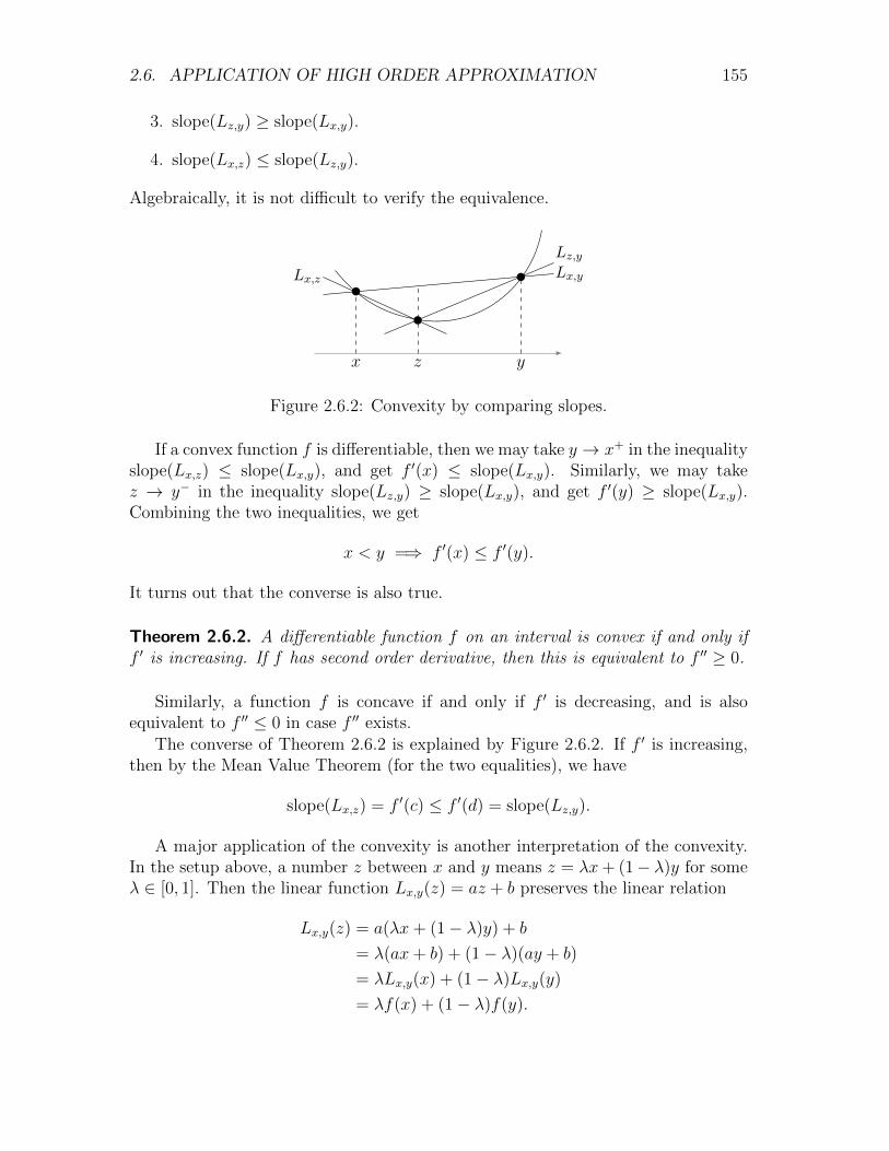
2.6. APPLICATION OF HIGH ORDER APPROXIMATION 155
3. slope(Lz,y) ≥ slope(Lx,y).
4. slope(Lx,z) ≤ slope(Lz,y).
Algebraically, it is not difficult to verify the equivalence.
x z y
Lx,yLx,z
Lz,y
Figure 2.6.2: Convexity by comparing slopes.
If a convex function f is differentiable, then we may take y → x+ in the inequalityslope(Lx,z) ≤ slope(Lx,y), and get f ′(x) ≤ slope(Lx,y). Similarly, we may takez → y− in the inequality slope(Lz,y) ≥ slope(Lx,y), and get f ′(y) ≥ slope(Lx,y).Combining the two inequalities, we get
x < y =⇒ f ′(x) ≤ f ′(y).
It turns out that the converse is also true.
Theorem 2.6.2. A differentiable function f on an interval is convex if and only iff ′ is increasing. If f has second order derivative, then this is equivalent to f ′′ ≥ 0.
Similarly, a function f is concave if and only if f ′ is decreasing, and is alsoequivalent to f ′′ ≤ 0 in case f ′′ exists.
The converse of Theorem 2.6.2 is explained by Figure 2.6.2. If f ′ is increasing,then by the Mean Value Theorem (for the two equalities), we have
slope(Lx,z) = f ′(c) ≤ f ′(d) = slope(Lz,y).
A major application of the convexity is another interpretation of the convexity.In the setup above, a number z between x and y means z = λx+ (1− λ)y for someλ ∈ [0, 1]. Then the linear function Lx,y(z) = az + b preserves the linear relation
Lx,y(z) = a(λx+ (1− λ)y) + b
= λ(ax+ b) + (1− λ)(ay + b)
= λLx,y(x) + (1− λ)Lx,y(y)
= λf(x) + (1− λ)f(y).

156 CHAPTER 2. DIFFERENTIATION
x z yc d
Lx,zLz,y
Figure 2.6.3: Increasing f ′(x) implies convexity.
Therefore the convexity means
f(λx+ (1− λ)y) ≤ λf(x) + (1− λ)f(y) for any 0 ≤ λ ≤ 1.
The following generalizes the inequality.
Theorem 2.6.3 (Jensen’s inequality). If f is convex, and
λ1 + λ2 + · · ·+ λn = 1, 0 ≤ λ1, λ2, . . . , λn ≤ 1,
then
f(λ1x1 + λ2x2 + · · ·+ λnxn) ≤ λ1f(x1) + λ2f(x2) + · · ·+ λnf(xn).
By reversing the direction of inequality, we also get Jensen’s inequality for con-cave functions.
In all the discussions about convexity, we may also consider the strict inequalities.So we have a concept of strict convexity, and a differentiable function is strictlyconvex on an interval if and only if its derivative is strictly increasing. Jensen’sinequality can also be extended to the strict case.
Example 2.6.5. By (xp)′′ = p(p − 1)xp−2, we know xp is convex on (0,+∞) whenp ≥ 1 or p < 0, and is concave when 0 < p ≤ 1.
For p ≥ 1, Jensen’s inequality means that
(λ1x1 + λ2x2 + · · ·+ λnxn)p ≤ λ1xp1 + λ2x
p2 + · · ·+ λnx
pn.
In particular, if all λi =1
n, then we get(
x1 + x2 + · · ·+ xnn
)p≤ xp1 + xp2 + · · ·+ xpn
n, for p ≥ 1, xi ≥ 0.
This means that the p-th power of the average is smaller than the average of thep-th power.

2.6. APPLICATION OF HIGH ORDER APPROXIMATION 157
We note that (xp)′′ > 0 for p > 1. Therefore all the inequalities are strict,provided some xi > 0 and 0 < λi < 1.
By replacing p withp
qand replacing xi with xqi , we get
(xq1 + xq2 + · · ·+ xqn
n
) 1q
≤(xp1 + xp2 + · · ·+ xpn
n
) 1p
, for p > q > 0.
x
1
x2
x12
x−12
x−1
x−2
Figure 2.6.4: xp for various p.
Example 2.6.6. By (log x)′′ = − 1
x2< 0, the logarithmic function is concave. Then
Jensen’s inequality tells us that
log(λ1x1 + λ2x2 + · · ·+ λnxn) ≥ λ1 log x1 + λ2 log x2 + · · ·+ λn log xn.
This is the same as
λ1x1 + λ2x2 + · · ·+ λnxn ≥ xλ11 x
λ22 · · · xλnn .
For the special case λi =1
n, we get
x1 + x2 + · · ·+ xnn
≥ n√x1x2 · · ·xn.
In other words, the arithmetic mean is bigger than the geometric mean.
Exercise 2.6.6. Study the convexity.

158 CHAPTER 2. DIFFERENTIATION
1. x3 + ax+ b.
2. x+ x53 .
3. x+ xp.
4. (x2 + 1)ex.
5. e−x2.
6.√x2 + 1.
7.1
x2 + 1.
8.x2 − 1
x2 + 1.
9. log(x2 + 1).
10. xx.
11. x+ 2 sinx.
12. x sin(log x).
Exercise 2.6.7. Find the condition on A and B so that the function
f(x) =
{Axp, if x ≥ 0,
B(−x)q, if x < 0,
is convex. Is the function necessarily differentiable at 0?
Exercise 2.6.8. Let p, q > 0 satisfy1
p+
1
q= 1. Use the concavity of log x to prove Young’s
inequality1
pxp +
1
qyq ≥ xy.
Exercise 2.6.9. For the case λ1 6= 1, Find suitable µ2, . . . , µn satisfying
λ1x1 + λ2x2 + · · ·+ λnxn = λ1x1 + (1− λ1)(µ2x2 + · · ·+ µnxn).
Then prove Jensen’s inequality by induction.
Exercise 2.6.10. Use the concavity of log x to prove that, for xi > 0, we have
x1 log x1 + x2 log x2 + · · ·+ xn log xnx1 + x2 + · · ·+ xn
≤ logx2
1 + x22 + · · ·+ x2
n
x1 + x2 + · · ·+ xn≤ log(x1 + x2 + · · ·+ xn).
Exercise 2.6.11. Use Exercise 2.6.10 to show that f(p) = log(xp1 + xp2 + · · · + xpn)1p is
decreasing. Then explain
(xq1 + xq2 + · · ·+ xqn)1q ≥ (xp1 + xp2 + · · ·+ xpn)
1p , for p > q > 0.
Note that the similar inequality in Example 2.6.5 is in reverse direction.
Exercise 2.6.12. Verify the convexity of x log x and then use the property to prove theinequality (x+ y)x+y ≤ (2x)x(2y)y. Can you extend the inequality to more variables?
2.6.3 Sketch of Graph
We have learned the increasing and decreasing properties, and the convex and con-cave properties. We may also pay attention to the symmetry properties such as evenor odd function, and the periodic property. Moreover, we should pay attention tothe following special points.

2.6. APPLICATION OF HIGH ORDER APPROXIMATION 159
1. Intercepts, where the graph of function intersects the axes.
2. Disruptions, where the functions are not continuous, or not differentiable.
3. Local extrema, which is often (but not restricted to) the places where thefunction changes between increasing and decreasing.
4. Points of inflection, which is the place where the function changes betweenconvex and concave.
5. Infinity, including the finite places where the function tends to infinity, andthe behavior of the function at the infinity.
One infinity behavior is the asymptotes of a function. If a linear function a+ bxsatisfies
limx→+∞
(f(x)− a− bx) = 0,
then the linear function is an asymptote at +∞. If b = 0, then the line is a horizontalasymptote. We also have similar asymptote at −∞ (perhaps with different a andb). Moreover, if limx→x0 f(x) = ∞ at a finite x0, then the line x = x0 is a verticalasymptote.
In subsequent examples, we sketch the graphs of functions and try to indicatethe characteristics listed above as much as possible.
Example 2.6.7. In Example 2.3.4, we determined the monotone property and thelocal extrema of f(x) = x3 − 3x + 1. The second order derivative f ′′(x) = 6x alsotells us that f(x) is concave on (−∞, 0] and convex on [0,+∞), which makes 0 intoa point of inflection. Moreover, the function has no asymptotes. The function isalso symmetric with respect to the point (0, 1) (f(x)− 1 is an odd function). Basedon these information, we may sketch the graph.
x (−∞,−1) −1 (−1, 0) 0 (0, 1) 1 (1,+∞)f = x3 − 3x+ 1 −∞← 3 0 −1 → +∞
f ′ = 3(x+ 1)(x− 1)+ 0 − 0 +↗ max ↘ min ↗
f ′′ = 6x+ 0 −
infl
Example 2.6.8. In Example 2.3.6, we determined the monotone property of f(x) =3√x2(x+1). The second order derivative f ′′(x) =
2(5x− 1)
93√x4
implies that the function
is concave on (−∞, 0) and on
(0,
1
5
], convex on
[1
5,+∞
), with
1
5as a point of
inflection. Moreover, we have limx→−∞ f(x) = −∞, limx→+∞ f(x) = +∞. The
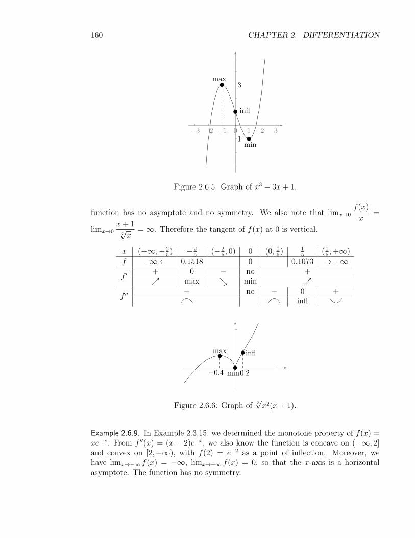
160 CHAPTER 2. DIFFERENTIATION
−3 −2 −1 0 1 2 3
3
1min
max
infl
Figure 2.6.5: Graph of x3 − 3x+ 1.
function has no asymptote and no symmetry. We also note that limx→0f(x)
x=
limx→0x+ 1
3√x
=∞. Therefore the tangent of f(x) at 0 is vertical.
x (−∞,−25) −2
5(−2
5, 0) 0 (0, 1
5) 1
5(1
5,+∞)
f −∞← 0.1518 0 0.1073 → +∞
f ′+ 0 − no +↗ max ↘ min ↗
f ′′− no − 0 +
infl
max infl
−0.4 0.2min
Figure 2.6.6: Graph of3√x2(x+ 1).
Example 2.6.9. In Example 2.3.15, we determined the monotone property of f(x) =xe−x. From f ′′(x) = (x − 2)e−x, we also know the function is concave on (−∞, 2]and convex on [2,+∞), with f(2) = e−2 as a point of inflection. Moreover, wehave limx→−∞ f(x) = −∞, limx→+∞ f(x) = 0, so that the x-axis is a horizontalasymptote. The function has no symmetry.

2.6. APPLICATION OF HIGH ORDER APPROXIMATION 161
1 2
e−12e−2max infl
Figure 2.6.7: Graph of xe−x.
Example 2.6.10. In Example 2.3.7, we determined the monotone property and the
local extrema of f(x) =x3
x2 − 1. The function is not defined at ±1, and has limits
limx→1±
f(x) = ±∞, limx→−1±
f(x) = ∓∞.
These give vertical asymptotes at ±1. Moreover, we have
limx→∞
(f(x)− x) = 0.
Therefore y = x is a slant asymptote at ∞.
The second order derivative f ′′(x) =2x(x2 + 3)
(x2 − 1)3shows that the function is convex
on (−1, 0), (1,+∞), and is concave at the other two intervals. Therefore 0 is a pointof inflection.
We also know the function is odd. So the graph is symmetric with respect tothe origin.
Exercise 2.6.13. Use the graph of x3 − 3x+ 1 in Example 2.6.7 to sketch the graphs.
1. −x3 + 3x2 − 1.
2. x3 − 3x+ 2.
3. |x3 − 3x+ 1|.
4. x3 − 3x.
5. x3 − bx, b > 0.
6. ax3 − bx+ c, ab > 0.
Exercise 2.6.14. Use the graph of xe−x in Example 2.6.9 to sketch the graphs.
1. xex.
2. xe2x.
3. (x+ 1)ex.
4. (ax+ b)ex.
5. xax.
6. |x|e−|x−1|.
Exercise 2.6.15. Sketch the graphs.

162 CHAPTER 2. DIFFERENTIATION
√3
−√
3
max
min
infl
Figure 2.6.8: Graph ofx3
x2 − 1.
1. x− sinx.
2. |x− sinx|.
3. x− cosx.
4. x+ sinx.
5. x+ cosx.
6.1
2+ sinx cosx.
Exercise 2.6.16. Sketch the graphs.
1.1
x2. 2.
1
x2 + 1. 3.
1
x2 − 1. 4.
1
x2 + bx+ c.
Exercise 2.6.17. Sketch the graphs.
1. (x2 + 1)p. 2. (x2 − 1)p. 3.√
1− x2. 4.√ax2 + bx+ c.
Exercise 2.6.18. Sketch the graph ofax+ b
cx+ dby using the graph of
1
x.
Exercise 2.6.19. Sketch the graphs on the natural domains of definitions.
1. x4 − 2x2 + 1.
2. x+1
x.
3.x
x2 + 1.
4.x3
(x− 1)2.
5. x√x− 1.
6.√x2 + 1− x.
7. x13 (1− x)
23 .
8. x2e−x.
9.1
1 + ex.
10. e1x .
11. x log x.
12. x− log(1 + x).
13. log(1− log x).
14. log(1 + x4).
15. e−x sinx.

2.7. NUMERICAL APPLICATION 163
16. x tanx. 17.1
1 + sin2 x. 18. 2 sinx+ sin 2x.
19. 2x− 4 sinx+ sin 2x.
2.7 Numerical Application
The linear approximation can be used to find approximate values of functions.
Example 2.7.1. The linear approximation of√x at x = 4 is
L(x) =√
4 + (√x)′|x=4(x− 4) = 2 +
1
4(x− 4).
Therefore the value of the square root near 4 can be approximately computed
√3.96 ≈ 2 +
1
4(−0.04) = 1.99,
√4.05 ≈ 2 +
1
4(0.05) = 2.0125.
Example 2.7.2. Assume some metal balls of radius r = 10 are selected to make aball bearing. If the radius is allowed to have 1% relative error, what is the maximalrelative error of the weight?
The weight of the ball is
W =4
3ρπr3.
where ρ is the density. The error ∆W of the weight caused by the error ∆r of theradius is
∆W ≈ dW
dr∆r = 4ρπr2∆r.
Therefore the relative error is∆W
W≈ 3
∆r
r.
Given the relative error of the radius is no more than 1%, we have
∣∣∣∣∆rr∣∣∣∣ ≤ 1%, so
that the relative error of the weight is
∣∣∣∣∆WW∣∣∣∣ ≤ 3%.
Example 2.7.3. In Example 2.2.11, we computed the derivatives of the functionsy = y(x) and z = z(x) given by the equations x2 + y2 + z2 = 2 and x + y + z = 0,which is really a circle in R3. The point P = (1, 0,−1) lies on the circle, where wehave
y(1) = 0, z(1) = −1, y′(1) =1− (−1)
(−1)− 0= −2, z′(1) =
1− 0
0− (−1)= 1.

164 CHAPTER 2. DIFFERENTIATION
Therefore
y(1.01) ≈ 0− 2 · 0.01 = −0.02, z(1.01) ≈ −1 + 1 · 0.01 = −0.99,
y(0.98) ≈ 0− 2 · (−0.02) = 0.04, z(0.98) ≈ −1 + 1 · (−0.02) = −1.02.
In other words, the points (1.01,−0.01,−0.99) and (0.98, 0.04,−1.02) are near (1, 0,−1)and almost on the circle.
Exercise 2.7.1. For a > 0 and small x, derive
n√an + x ≈ a+
x
nan−1.
Then find the approximate values.
1. 4√
15. 2.√
46. 3. 5√
39. 4. 7√
127.
Exercise 2.7.2. The period of a pendulum is T = 2π
√L
g, where L the length of the
pendulum and g is the gravitational constant. If the length of the pendulum is increasedby 0.4%, what is the change in the period?
2.7.1 Remainder Formula
We may get more accurate values by using high order approximations. On the otherhand, we have more confidence on the estimated values if we also know what theerror is. The following result gives a formula for the error.
Theorem 2.7.1 (Lagrange Form of the Remainder). If f(x) has (n + 1)-st orderderivative on (a, x), then the remainder of the n-th order Taylor expansion of f(x)at a is
Rn(x) =f (n+1)(c)
(n+ 1)!(x− a)n+1 for some c ∈ (a, x).
We only illustrate the argument for the case n = 2. We know that the remaindersatisfies R(a) = R′(a) = R′′(a) = 0. Therefore by Cauchy’s Means Value Theorem(Theorem 2.4.5), we have
R2(x)
(x− a)3=
R2(x)−R2(a)
(x− a)3 − (a− a)3=
R′2(c1)
3(c1 − a)2(a < c1 < x)
=R′2(c1)−R′2(a)
3[(c1 − a)2 − (a− a)2]=
R′′2(c2)
3 · 2(c2 − a)(a < c2 < c1)
=R′′2(c2)−R′′2(a)
3 · 2(c2 − a)=R′′′2 (c3)
3 · 2 · 1=f ′′′(c3)
3!. (a < c3 < c2)
In the last step, we use R′′′2 = f ′′′ because the f − R2 is a quadratic function andhas vanishing third order derivative.

2.7. NUMERICAL APPLICATION 165
A slight modification of the proof above actually gives a proof that the Taylorexpansion is high order approximation (Theorem 2.5.2).
Example 2.7.4. The error for the linear approximation in Example 2.7.1 can be esti-mated by
R1(x) = −
1
4c32
2!∆x2 =
1
8c32
∆x3.
For both approximate values, we have
|R1| ≤1
8 · 4 32
0.052 = 0.0000390625 < 4× 10⁻⁵.
If we use the quadratic approximation at 4
√x ≈ 2 +
1
4(x− 4)− 1
64(x− 4)2,
then we get better estimated values
√3.96 ≈ 2 +
1
4(−0.04)− 1
64(−0.04)2 = 1.989975,
√4.05 ≈ 2 +
1
4(0.05)− 1
64(0.05)2 = 2.0124609375.
The error can be estimated by
R2(x) =
3
8c52
3!∆x3 =
1
16c52
∆x3.
For both computations, we have
|R2| ≤1
16 · 4 52
0.053 = 0.00000025 = 2.5× 10⁻⁷.
The true values are√
3.96 = 1.989974874213 · · · and√
4.05 = 2.01246117975 · · · .
Example 2.7.5. The Taylor expansion of ex tells us
e = e1 = 1 +1
1!+
1
2!+ · · ·+ 1
n!+Rn(1).
By
|Rn(1)| = ec
(n+ 1)!1n+1 ≤ e
(n+ 1)!, 0 < c < 1,
we know|R13(1)| ≤ 0.000000000035 = 3.5× 10⁻¹¹.

166 CHAPTER 2. DIFFERENTIATION
On the other hand,
1 +1
1!+
1
2!+ · · ·+ 1
13!= 2.718281828447 · · · ,
Therefore e = 2.7182818284 · · · .
Exercise 2.7.3. Find approximate values by using Taylor expansions and estimate the er-rors.
1. sin 1, 3rd order approximation.
2. log 2, 5th order approximation.
3. e−1, 5th order approximation.
4. arctan 2, 3rd order approximation.
Exercise 2.7.4. Find approximate values accurate up to the 10-th digit.
1. sin 1. 2.√
4.05. 3. e−1. 4. tan 46◦.
Exercise 2.7.5. Find the approximate value of tan 1 accurate up to the 10-th digit by usingthe Taylor expansions of sinx and cosx.
Exercise 2.7.6. If we use the Taylor expansion to calculate e accurate up to the 100-thdigit, what is the order of the Taylor expansion we should use?
2.7.2 Newton’s Method
The linear approximation can also be used to find approximate solutions of equa-tions. To solve f(x) = 0, we start with a rough estimation x0 and consider the linearapproximation at x0
L0(x) = f(x0) + f ′(x0)(x− x0).
We expect the solution of the linear equation L0(x) = 0 to be very close to thesolution of f(x) = 0. The solution of the linear equation is easy to find
x1 = x0 −f(x0)
f ′(x0).
Although x1 is not the exact solution of f(x) = 0, chances are it is an improvementof the initial estimation x0.
To get an even better approximate solution, we repeat the process and considerthe linear approximation at x1
L1(x) = f(x1) + f ′(x1)(x− x1)
The solution of the linear equation L1(x) = 0
x2 = x1 −f(x1)
f ′(x1)

2.7. NUMERICAL APPLICATION 167
solution
L0 L1 L2 L3
x0 x1 x2 x3
Figure 2.7.1: Newton’s method.
is an even better estimation than x1. The idea leads to an inductively constructedsequence
xn+1 = xn −f(xn)
f ′(xn).
We expect the sequence to rapidly converge to the exact solution of f(x) = 0.
The scheme above for finding the approximate solution is called the Newton’smethod. The method may fail for various reasons. However, if the function is rea-sonably good and the initial estimation x0 is sufficiently close to the exact solution,then the method indeed produces a sequence that rapidly converges to the exactsolution. In fact, the error between xn and the exact solution c satisfies
|xn+1 − c| ≤M |xn − c|2
for some constant M that depends only on the function.
Example 2.7.6. By Example 1.7.5, the equation x3−3x+1 = 0 should have a solutionon (0.3, 0.4). By Example 1.7.6, the equation should also have a second solution > 1and a third solution < 0. More precisely, by f(−2) = −1, f(−1) = 3, f(1) = −1,f(2) = 3, the second solution is on (−2,−1) and the third solution is on (1, 2).Taking −2, 0.3, 2 as initial estimations, we apply Newton’s method and computethe sequence
xn+1 = xn −x3n − 3xn + 1
3(x2n − 1)
=2
3xn +
2xn − 1
3(x2n − 1)
.
We find the three solutions
−1.87938524157182 · · · , 0.347296355333861 · · · , 1.53208888623796 · · · .

168 CHAPTER 2. DIFFERENTIATION
n x0 = −2 x0 = 0.3 x0 = 21 -1.88888888888889 0.346520146520147 1.666666666666672 -1.87945156695157 0.347296117887934 1.548611111111113 -1.87938524483667 0.347296355333838 1.532390161865384 -1.87938524157182 0.347296355333861 1.532088989397225 -1.87938524157182 0.347296355333861 1.532088886237976 1.532088886237967 1.53208888623796
Note that the initial estimation cannot be 1 or −1, because the derivative van-ishes at the points. Moreover, if we start from 0.88, 0.89, 0.90, we get very differentsequences that respectively converge to the three sequences. We see that Newton’smethod can be very sensitive to the initial estimation, especially when the estimationis close to where the derivative vanishes.
n x0 = 0.88 x0 = 0.89 x0 = 0.901 -0.5362647754137 -0.657267917268 -0.803508771929832 0.6122033746535 0.920119732577 1.916557891161113 0.2884916149262 -1.212642459862 1.630979985462524 0.3461342508923 -3.235117846394 1.541502632357255 0.3472958236620 -2.419800571908 1.532187945055096 0.3472963553337 -2.014098301161 1.532088897394467 0.3472963553339 -1.891076746708 1.532088886237968 -1.8794853750609 -1.879385249013
10 -1.879385241572
Example 2.7.7. We solve the equation sinx+x cosx = 0 by starting with the estima-tion x0 = 1. After five steps, we find the exact solution should be 0.325639452727856 · · · .
n xn0 1.0000000000000001 0.4719246675054872 0.3309688263458733 0.3256453120765424 0.3256394527348765 0.3256394527278566 0.325639452727856
Exercise 2.7.7. Applying Newton’s method to solve x3− x− 1 = 0 with the initial estima-tions 1, 0.6 and 0.57. What lesson can you draw from the conclusion?
Exercise 2.7.8. Use Newton’s method to find the unique positive root of f(x) = ex−x−2.

2.7. NUMERICAL APPLICATION 169
Exercise 2.7.9. Use Newton’s method to find all the solutions of x2 − cosx = 0.
Exercise 2.7.10. Use Newton’s method to find the approximate values of√
4.05 and e−1
accurate up to the 10-th digit.
Exercise 2.7.11. Use Newton’s method to find all solutions accurate up to the 6-th digit.
1. x4 = x+ 3. 2. ex = 3− 2x. 3. cos2 x = x. 4. x+ tanx = 1.
Note that one may rewrite the equation into another equivalent form and derive asimpler recursive relation.
Exercise 2.7.12. The ancient Babylonians used the recursive relation
xn+1 =1
2
(xn +
a
xn
)to get more an more accurate approximate values of
√a. Explain the scheme by Newton’s
method.
Exercise 2.7.13. What approximate values does the recursive relation xn+1 = 2xn − ax2n
give you? Explain by Newton’s method.
Exercise 2.7.14. Explain why Newton’s method does not work if we try to solve x3−3x+1 =0 by starting at the estimation 1.
Exercise 2.7.15. Newton’s method fails to solve the following equations by starting at anyx0 6= 0. Why?
1. 3√x = 0. 2. sign(x)
√|x| = 0.

170 CHAPTER 2. DIFFERENTIATION

Chapter 3
Integration
3.1 Area and Definite Integral
3.1.1 Area below Non-negative Function
Let f(x) be a non-negative function on [a, b]. We wish to find the area of the region
G[a,b](f) = {(x, y) : a ≤ x ≤ b, 0 ≤ y ≤ f(x)}
between the graph of the function and the x-axis.
a
f
b
G[a,b](f)
Figure 3.1.1: The region between the function and the x-axis.
Our strategy is the following. For any x ∈ [a, b], let A(x) be the area of G[a,x](f),which is part of the region over [a, x]. We will find how the function A(x) changesand recover A(x) from its change. The area we wish to find is then the value A(b).The subsequent argument assumes that f(x) is continuous.
Consider an interval [x, x+h] ⊂ [a, b], which implicitly assumes h > 0. Then thechange A(x+h)−A(x) is the area of G[x,x+h](f). Note that G[x,x+h](f) is sandwichedbetween two rectangles
[x, x+ h]× [0,m] ⊂ G[x,x+h](f) ⊂ [x, x+ h]× [0,M ],
171

172 CHAPTER 3. INTEGRATION
wherem = min
[x,x+h]f, M = max
[x,x+h]f.
Since bigger region should have bigger area, we have
mh ≤ A(x+ h)− A(x) ≤Mh.
By h > 0, this is the same as
m ≤ A(x+ h)− A(x)
h≤M. (3.1.1)
Since the (right) continuity of f(x) implies
limh→0+
m = f(x) = limh→0+
M,
by the sandwich rule, we further get the right derivative
A′+(x) = limh→0+
A(x+ h)− A(x)
h= f(x). (3.1.2)
a
f
b
m
x
M
x+ h
G[x,x
+h
](f
)
Figure 3.1.2: Estimate the change of area.
The argument above assumes h > 0. For h < 0, we consider [x + h, x] ⊂ [a, b].Then the change A(x+ h)−A(x) is the negative of the area of G[x+h,x](f), and theinterval [x+ h, x] has length −h. By the same reason as before, we get
m(−h) ≤ −(A(x+ h)− A(x)) ≤M(−h).
By−h > 0, we still get the inequality (3.1.1), and further application of the sandwichrule gives the left derivative
A′−(x) = limh→0−
A(x+ h)− A(x)
h= f(x).
We conclude that, for non-negative and continuous f(x), we have
A′(x) = f(x). (3.1.3)

3.1. AREA AND DEFINITE INTEGRAL 173
Example 3.1.1. To find the area of the region below f(x) = c over [a, b], by (3.1.3),we have A′(x) = c = (cx)′. Then by Theorem 2.4.3, we get A(x) = cx+C. Furtherby A(a) = 0, we get C = −ca and A(x) = c(x−a). Therefore the area of the regionis A(b) = c(b− a).
The region G[a,b](c) is actually a rectangle of base b − a and height c. Thecomputation of the area is consistent with the common sense.
Example 3.1.2. To find the area of the region below f(x) = x over [0, a], we start
with A′(x) = x =
(1
2x2
)′. This implies A(x) =
1
2x2 + C. By A(0) = 0, we further
get C = 0 and A(x) =1
2x2. Therefore the region has area A(a) =
1
2a2.
The region is actually a triangle, more precisely half of the square of side lengtha. The computation of the area is consistent with the common sense.
The pattern we see from the examples above is that, to find the area below a non-negative function and over an interval [a, b], we first find a function F (x) satisfyingf(x) = F ′(x). Then by Theorem 2.4.3, A′(x) = F ′(x) implies A(x) = F (x) + C.Further, by A(a) = 0, we get C = −F (a). Therefore A(x) = F (x)− F (a), and thearea we wish to find is
Area(G[a,b](f)) = F (b)− F (a).
This is the Newton-Leibniz formula. The function F is naturally called an an-tiderivative of f .
Example 3.1.3. To find the area of the region below x2 and over [0, a], we use(1
3x3
)′= x2. The area is
1
3a3 − 1
303 =
1
3a3.
More generally, for any p 6= −1 and 0 < a < b, by
(1
p+ 1xp)′
= xp, the area of
the region below xp and over [a, b] is
1
p+ 1(bp+1 − ap+1).
For example, the area of the region below√x and over [1, 2] is
2
3x
32
∣∣∣∣x=2
x=1
=2
3(2
32 − 1
32 ) =
2
3(2√
2− 1).
Exercise 3.1.1. Find the area of the region below the function over the given interval.

174 CHAPTER 3. INTEGRATION
1 2
√x
Figure 3.1.3: Area below parabola is2
3(2√
2− 1).
1. xp on [0, 1], p > 0.
2. sinx on [0, π2 ].
3. ex on [0, a].
4.1
xon [1, a].
5.√
1 + x on [1, 2].
6. log x on [1, a].
Exercise 3.1.2. Find the area of the region bounded by 1− x2 and the x-axis.
3.1.2 Definite Integral of Continuous Function
What do we get if we apply the Newton-Leibniz formula to general continuousfunctions, which might become negative somewhere? The answer is the signed area.This means that we count the region between the non-negative part of f and thex-axis as having positive area and count the region between the non-positive partof f and the x-axis as having negative area. See Figure 3.1.4.
f
−
+
Figure 3.1.4: Computation by the Newton-Leibniz formula gives signed area.
To justify our claim, let A(x) be the signed area for f(x) over [a, x]. What weare really concerned with is the change of A(x) where f is negative. So we consider[x, x+ h] ⊂ [a, b], with h > 0 and f < 0 on [x, x+ h]. The change A(x+ h)− A(x)is the negative of the positive, “unsigned” area of the region
G[x,x+h](f) = {(t, y) : x ≤ t ≤ x+ h, 0 ≥ y ≥ f(t)}
between f and the x-axis along the interval [x, x+h]. We have the similar inclusion

3.1. AREA AND DEFINITE INTEGRAL 175
(see Figure 3.1.5, and note that [M, 0] ⊂ [m, 0] because 0 ≥M ≥ m)
[x, x+ h]× [M, 0] ⊂ G[x,x+h](f) ⊂ [x, x+ h]× [m, 0], m = min[x,x+h]
f,M = max[x,x+h]
f.
The heights of the rectangles are respectively −M and −m, and we get (beware ofthe signs)
(−M)h ≤ −(A(x+ h)− A(x)) ≤ (−m)h.
Again we get the inequality (3.1.1) and subsequently the limit (3.1.2).The discussion for the case h < 0 is similar, and we conclude that A′(x) = f(x).
a
f
b
x
m
M
x+ h
G(f
)
Figure 3.1.5: Estimate the change of negative area.
The signed area is the definite integral of f(x) and is denoted
∫ b
a
f(x)dx. The
function f(x) is called the integrand and the ends a, b of the interval are calledthe upper limit and lower limit. The argument above and the explanation beforeExample 3.1.3 show that the definite integral can be computed by the Newton-Leibniz formula ∫ b
a
f(x)dx = F (b)− F (a), where F ′(x) = f(x).
Example 3.1.4. By (x)′ = 1 and
(1
2x2
)′= x, we get
∫ b
a
dx = b− a,∫ b
a
xdx =1
2(b2 − a2).
In general, for any integer n 6= −1, we have∫ b
a
xndx =1
n+ 1(bn+1 − an+1).
However, for n < 0, a and b need to have the same sign. The reason is that wederived the Newton-Leibniz formula under the assumption that the integrand is

176 CHAPTER 3. INTEGRATION
continuous. If a and b have different sign, then 0 ∈ [a, b], and xn is not continuouson [a, b] for n < 0.
On the other hand, for any p, xp is defined for x > 0. Then for b ≥ a > 0, wehave ∫ b
a
xpdx =1
p+ 1(bp+1 − ap+1).
We note that xp is also defined at 0 for p ≥ 0, and the formula above holds forp ≥ 0 and b ≥ a ≥ 0. The reason is that xp is right continuous at 0, and we derivedNewton-Leibniz formula by one-sided derivatives.
Example 3.1.5. By (ex)′ = ex and (log x)′ =1
x, we get∫ b
a
exdx = eb − ea,∫ b
a
dx
x= log b− log a = log
b
a.
Note that the second integral requires b ≥ a > 0.
Example 3.1.6. By (sin x)′ = cosx and (cos x)′ = − sinx, we get∫ b
a
cosxdx = sin b− sin a,
∫ b
a
sinxdx = cos a− cos b.
For example, we have ∫ 0
−πsinxdx = cos(−π)− cos 0 = −2.
Example 3.1.7. From the derivatives of arcsinx and arctanx, we get∫ b
a
dx√1− x2
= arcsin b− arcsin a,
∫ b
a
dx
1 + x2= arctan b− arctan a.
Of course, we need |a|, |b| < 1 in the first equality because the integrand is defined
only on the open interval (−1, 1). In particular, the area of the region below1
1 + x2
and over [0, 1] is ∫ 1
0
dx
1 + x2= arctan 1− arctan 0 =
π
4.
We also note that
lima→−∞b→+∞
∫ b
a
dx
1 + x2= lim
b→+∞arctan b− lim
a→−∞arctan a =
π
2−(−π
2
)= π.
So the area of the unbounded region between1
1 + x2and the x-axis is π.
Exercise 3.1.3. Use the area meaning of definite integral to directly find the value.

3.1. AREA AND DEFINITE INTEGRAL 177
1.
∫ 1
−1
√1− x2dx. 2.
∫ 3
0(x− 2)dx. 3.
∫ b
a|x− 1|dx.
Exercise 3.1.4. Compute and compare∫ 2
0x3dx,
∫ 2
0x5dx,
∫ 2
04x3dx,
∫ 2
06x5dx,
∫ 2
0(4x3 + 6x5)dx.
What can you observe about the relation between∫ b
af(x)dx,
∫ b
ag(x)dx,
∫ b
acf(x)dx,
∫ b
a(f(x) + g(x))dx.
Exercise 3.1.5. Compute definite integral.
1.
∫ 2
−1(x2 − 3x− 4)dx.
2.
∫ 2
0(3x+ 1)2dx.
3.
∫ 2
0(3x+ 1)(x− 3)dx.
4.
∫ 8
0
√3x+ 1dx.
5.
∫ 1
0(3 + x
√x)dx.
6.
∫ 2
1
(x+
1
x
)2
dx.
7.
∫ b
0ex+adx.
8.
∫ 1
0(e−x + sinπx)dx.
9.
∫ π4
0secx tanxdx.
Exercise 3.1.6. For non-negative integers m and n, prove that∫ 2π
0cosmx sinnxdx = 0;
∫ 2π
0cosmx cosnxdx =
0, if m 6= n,
π, if m = n 6= 0,
2π, if m = n = 0;∫ 2π
0sinmx sinnxdx =
{0, if m 6= n or m = n = 0,
π, if m = n 6= 0.
Exercise 3.1.7. Compute
∫ b
a
3√xdx and
∫ b
a
13√xdx. Explain for what range of a, b are the
formulae valid.
Exercise 3.1.8. What is wrong with the equality?
1.
∫ 1
−1
1
x2dx = −1
x
∣∣∣∣x=1
x=−1
= 2. 2.
∫ π
0sec2 xdx = tanπ − tan 0 = 0.
Exercise 3.1.9. What is the area of the unbounded region between1√
1− x2and the x-axis,
over the interval (−1, 1)?

178 CHAPTER 3. INTEGRATION
3.1.3 Property of Area and Definite Integral
Since the definite integral is the signed area, the usual properties of area is reflectedas properties of the definite integral. An important property of area is the additivity.Specifically, if X ∩ Y has zero area, then the area of X ∪ Y should be the area of Xplus the area of Y . Translated to definite integral, this means∫ c
a
f(x)dx =
∫ b
a
f(x)dx+
∫ c
b
f(x)dx. (3.1.4)
The equality can be used to calculate the definite integral of “piecewise continuous”functions.
Example 3.1.8. The definite integral of the function (which is not continuous at 0)
f(x) =
{−2x, if − 1 ≤ x < 0,
ex, if 0 ≤ x ≤ 1,
on [−1, 1] is∫ 1
−1
f(x)dx =
∫ 0
−1
f(x)dx+
∫ 1
0
f(x)dx =
∫ 0
−1
(−2x)dx+
∫ 1
0
exdx
= −x2|0−1 + ex|10 = e.
1
ex
−1
−2x
Figure 3.1.6: Definite integral of a piecewise continuous function.
We note that the computation of
∫ 0
−1
f(x)dx actually reassigns the value f(0) = 0
to make the function continuous on [−1, 0]. The modification happens inside thevertical line x = 0. Since the vertical line has zero area, this does not affect thewhole integral.
In general, changing the value of the integrand at finitely many places does notaffect the integral.

3.1. AREA AND DEFINITE INTEGRAL 179
Presumably, the definite integral
∫ b
a
f(x)dx is defined only for the case a ≤ b,
and the equality (3.1.4) implicitly assumes a ≤ b ≤ c. However, by∫ a
a
f(x)dx = 0,
and by taking c = a in (3.1.4), we get∫ a
b
f(x)dx = −∫ b
a
f(x)dx.
This extends the definite integral to the case the upper limit is smaller than the lowerlimit. With such extension, the equality (3.1.4) holds for any combination of a, b, c.Moreover, the extended definite integral is still computed by the antiderivative asbefore.
Another important property of area is positivity. Translated into definite inte-gral, this means
f ≥ 0 =⇒∫ b
a
f(x)dx ≥ 0, for a < b. (3.1.5)
Note that if a > b, then
∫ b
a
f(x)dx ≤ 0. The positivity is further extended to
monotonicity in Example 3.5.5.If we shift the graph under f(x) over [a, b] by d, we get the graph under f(x−d)
over [a+ d, b+ d]. Since the area is not changed by shifting, we get∫ b+d
a+d
f(x− d)dx =
∫ b
a
f(x)dx. (3.1.6)
See Exercise for more examples of properties of area implying properties of definiteintegral.
In Section 3.5, we will introduce more properties from the the viewpoint ofcomputation (i.e., Newton-Leibniz formula). Some of these properties cannot beeasily explained by properties of area.
Exercise 3.1.10. Suppose
∫ 2
0f(x)dx = 3,
∫ 4
5f(x)dx = 2,
∫ 0
5f(x)dx = 0. Find
∫ 4
2f(x)dx.
Exercise 3.1.11. Use area to explain the equalities.
1.
∫ −a−b
f(−x)dx =
∫ b
af(x)dx.
2.
∫ b
acf(x)dx = c
∫ b
af(x)dx.

180 CHAPTER 3. INTEGRATION
3.
∫ b
af(cx)dx = c−1
∫ cb
caf(x)dx.
Then express
∫ b
af(Ax+B)dx as some multiple of the definite integral of f(x) over some
interval.
Exercise 3.1.12. Compute the integrals.
1.
∫ b
0axdx.
2.
∫ b
a(1 + 2x)ndx.
3.
∫ 2
−1sign(x)dx.
4.
∫ 2
−1x2sign(x)dx.
5.
∫ 2
−1|x|dx.
6.
∫ −1
2|x|dx.
7.
∫ 2
0|x2 − 3x+ 2|dx.
8.
∫ 2π
0| sinx|dx.
9.
∫ 0
2π| sinx|dx.
Exercise 3.1.13. Compute the integrals.
1.
∫ 2
0f(x)dx, f(x) =
{x2, if x < 1,
x−2, if x ≥ 2.
2.
∫ 2
−2f(x)dx, f(x) =
{e2|x|, if |x| < 1,
e−x, if |x| ≥ 1.
3.
∫ π
0f(x)dx, f(x) =
{sinx, if x < π
2 ,
cosx, if x ≥ π2 .
4.
∫ π
−πf(x)dx, f(x) =
{sinx, if |x| < π
2 ,
cosx, if |x| ≥ π2 .
3.2 Rigorous Definition of Integral
3.2.1 What is Area?
The definite integral is defined as the signed area. Therefore the rigorous definitionof integral relies on the rigorous definition of area. Any reasonable definition of areashould have the following three properties (the area of a subset X ⊂ R2 is denotedµ(X)):
1. Bigger subsets have bigger area: X ⊂ Y implies µ(X) ≤ µ(Y ).
2. Areas can be added: If µ(X ∩ Y ) = 0, then µ(X ∪ Y ) = µ(X) + µ(Y ).
3. Rectangles have the usual area: µ(〈a, b〉 × 〈c, d〉) = (b− a)(d− c).

3.2. RIGOROUS DEFINITION OF INTEGRAL 181
Here 〈a, b〉 can mean any of [a, b], (a, b), (a, b], or [a, b). A carefully review of theargument in Section 3.1 shows that nothing beyond the three properties are used.
Suppose a plane region A ⊂ R2 is a union of finitely many rectangles, A = ∪ni=1Ii,such that the intersections between Ii are at most lines. Since lines have zero areaby the third property, we may use the second property to further define µ(A) =∑n
i=1 µ(Ii). We give such a plane region the temporary name “good region”, sincewe have definite idea about the area of a good region. (Strictly speaking, we stillneed to argue that
∑ni=1 µ(Ii) is independent of the decomposition A = ∪ni=1Ii.)
Figure 3.2.1: Good region.
For any (bounded) subset X ⊂ R2, we may try to approximate X by goodregions, from inside as well as from outside. In other words, we consider goodregions A and B satisfying A ⊂ X ⊂ B. Then by the first property of area, we musthave
µ(A) ⊂ µ(X) ⊂ µ(B).
Note that µ(A) and µ(B) have been defined, and µ(X) is yet to be defined. So weintroduce the inner area (the maximum should really be the supremum)
µ∗(X) = max{µ(A) : A ⊂ X, A is a good region},
as the lower bound for µ(X), and the outer area (the minimum should really be theinfimum)
µ∗(X) = min{µ(B) : B ⊃ X, B is a good region},
as the upper bound for µ(X). We say that the subset X has area (or Jordanmeasurable) if µ∗(X) = µ∗(X), and the common value is the area µ(X) of X. Ifµ∗(X) 6= µ∗(X), then we say X has no area.
The subset X has area if and only if for any ε > 0, there are good regions Aand B, such that A ⊂ X ⊂ B and µ(B) − µ(A) < ε. In other words, we canfind good inner and outer approximations, such that the difference between theapproximations can be arbitrarily small.

182 CHAPTER 3. INTEGRATION
B
X
A
Figure 3.2.2: Approximation by good regions.
Example 3.2.1. A point can be considered as a reduced rectangle and has area 0. If Xconsists of finitely many points, then we can take B = X be the union of all “pointrectangles” in X. Since µ(B) = 0, we get µ∗(X) = 0. By 0 ≤ µ∗(X) ≤ µ∗(X), wealso have µ∗(X) = 0. Therefore finitely many points has area 0.
Example 3.2.2. Consider the triangle with vertices (0, 0), (1, 0) and (1, 1). We parti-tion the interval [0, 1] into n parts of equal length
[0, 1] = ∪ni=1
[i− 1
n,i
n
].
Correspondingly, we have the inner and outer approximations of the triangle
An = ∪ni=1
[i− 1
n,i
n
]×[0,i− 1
n
], Bn = ∪ni=1
[i− 1
n,i
n
]×[0,i
n
].
They have area
µ(An) =n∑i=1
1
n
i− 1
n=
1
2n(n− 1), µ(Bn) =
n∑i=1
1
n
i
n=
1
2n(n+ 1).
By taking sufficiently big n, the difference µ(Bn)−µ(An) =1
ncan be arbitrarily
small. Therefore the triangle has area, and the area is given by limn→∞ µ(An) =
limn→∞ µ(Bn) =1
2. This justifies the conclusion of Example 3.1.2 for the case a = 1.
Example 3.2.3. For an example of subsets without area, i.e., satisfying µ∗(X) 6=µ∗(X), let us consider the subset X = (Q ∩ [0, 1])2 of all rational pairs in the unitsquare.

3.2. RIGOROUS DEFINITION OF INTEGRAL 183
1
inner approx.
1
outer approx.
Figure 3.2.3: Approximating triangle.
Since the only rectangles contained in X are single points, any good regionA ⊂ X must be finitely many points. Therefore µ(A) = 0 for any good regionA ⊂ X, and µ∗(X) = 0.
On the other hand, if B is a good region containing X, then B must almostcontain the whole square [0, 1]2, with the only exception of finitely many horizontalor vertical (irrational) line segments. Therefore we have µ(B) ≥ µ([0, 1]2) = 1. Thisimplies µ∗(X) ≥ 1 (show that µ∗(X) = 1!).
Exercise 3.2.1. Use inner and outer approximations to explain that any rectangle has areagiven by the multiplication of two sides. This justifies Example 3.1.1.
Exercise 3.2.2. Explain that a (not necessarily horizontal or vertical) straight line segmenthas area 0.
Exercise 3.2.3. Explain that the region between y = x and the x-axis over [0, a] has area1
2a2. This fully justifies the computation in Example 3.1.2.
Exercise 3.2.4. Explain that the subset X = (Q∩ [0, 1])× [0, 1] of all vertical rational linesin the unit square has no area.
Exercise 3.2.5. Show that if X ⊂ Y , then µ∗(X) ≤ µ∗(Y ) and µ∗(X) ≤ µ∗(Y ). Inparticular, we have µ(X) ≤ µ(Y ) in case both X and Y have areas. The property is usedin deriving (3.1.1).
3.2.2 Darboux Sum
After the rigorous definition of area, we can give the rigorous definition of definiteintegral.
Definition 3.2.1. A function f(x) is Riemann integrable if the region
G[a,b](f) = {(x, y) : a ≤ x ≤ b, y is between 0 and f(x)}

184 CHAPTER 3. INTEGRATION
has area. Moreover, the Riemann integral is∫ b
a
f(x)dx = µ(G[a,b](f) ∩H+
)− µ
(G[a,b](f) ∩H−
),
whereH+ = {(x, y) : y ≥ 0}, H− = {(x, y) : y ≤ 0}
are the upper and lower half planes.
Suppose f ≥ 0 on [a, b]. As indicated by Figure 3.2.4, for any inner approxima-tion of G[a,b](f), we can always choose “full vertical strips” to get a better approxima-tion for G[a,b](f). Here better means closer to the expected value of µ(G[a,b](f)). Theouter approximations have similar improvements by full vertical strips. Thereforewe only need to consider the approximations by full vertical strips.
a b a bxi−1 xi
mi
Figure 3.2.4: Better inner approximations by vertical strips.
An approximation by full vertical strips is determined by a partition of the in-terval
P : a = x0 < x1 < · · · < xn = b.
On the i-th interval [xi−1, xi], the inner strip has height mi = min[xi−1,xi] f (the mini-mum should really be the infimum), and the outer strip has heightMi = max[xi−1,xi] f(the maximum should really be the supremum). Therefore the inner and outer ap-proximations are
AP = ∪ni=1[xi−1, xi]× [0,mi) ⊂ X ⊂ BP = ∪ni=1[xi−1, xi]× [0,Mi].
The areas of the two approximations are the lower and upper Darboux sums
L(P, f) = µ(AP ) =n∑i=1
mi(xi − xi−1),
U(P, f) = µ(BP ) =n∑i=1
Mi(xi − xi−1).
The Riemann integrability of f means that G[a,b](f) has area, which furthermeans that the difference between inner and outer approximations can be arbitrarilysmall. Therefore we get the following criterion for the integrability.

3.2. RIGOROUS DEFINITION OF INTEGRAL 185
Theorem 3.2.2 (Riemann Criterion). A bounded function f on [a, b] is Riemannintegrable, if and only if for any ε > 0, there is a partition P , such that
U(P, f)− L(P, f) =n∑i=1
(max
[xi−1,xi]f − min
[xi−1,xi]f
)(xi − xi−1) < ε.
The quantityω[xi−1,xi]f = max
[xi−1,xi]f − min
[xi−1,xi]f
measures how much the value of f fluctuates on [xi−1, xi] and is called the oscillationof the function on the interval. Since the continuity of a function can imply that suchoscillations are uniformly small, continuous functions are always Riemann integrable.The criterion also implies that monotone functions are Riemann integrable. On theother hand, there are functions that are not Riemann integrable.
Example 3.2.4. Consider the Dirichlet function D(x) on [0, 1]. We always have
min[xi−1,xi]
D = 0, max[xi−1,xi]
D = 1.
Therefore U(P, f)− L(P, f) = 1 cannot be arbitrarily small. We conclude that theDirichlet function is not Riemann integrable.
The example is closely related to Example 3.2.3. See Exercise 3.2.4.
We note that U(P, f) − L(P, f) is the area of the good subset BP − AP =∪ni=1[xi−1, xi]× [mi,Mi]. If we consider all the partitions P , the all such good subsetsare essentially all the outer approximations of the graph {(x, f(x)) : a ≤ x ≤ b} off (a curve, not including the part below f). Therefore Theorem 3.2.2 basically saysthat a function is Riemann integrable if and only if the graph curve of the functionhas zero area.
The graph curve is part of the boundary of G(f). In this viewpoint, Theorem3.2.2 is a special case of the following.
Theorem 3.2.3. A bounded subset X ⊂ R2 has area if and only if its boundary ∂Xhas zero area.
We remark that the theory of area can be easily extended to the theory ofvolume for subsets in Rn. We may then get the rigorous definition of multivariableRiemann integrals on subsets of Euclidean spaces, where the subsets should havevolume themselves. The high dimensional versions of Theorems 3.2.2 and 3.2.3 arestill valid.
Further extension of the area theory introduces countably many in place offinitely many. The result is the modern theory of Lebesgue measure and Lebesgueintegral.

186 CHAPTER 3. INTEGRATION
3.2.3 Riemann Sum
Suppose f is Riemann integrable. When the partition gets more and more refined,the upper and lower Darboux sums, as the areas of the outer and inner approxima-
tions, will become closer to the integral
∫ b
a
f(x)dx. Now choose φi satisfying
mi ≤ φi ≤Mi.
Then we get the Riemann sum
S(P, f) =n∑i=1
φi(xi − xi−1)
sandwiched between the two Darboux sums
L(P, f) ≤ S(P, f) ≤ U(P, f).
We conclude that S(P, f) will also become closer to the integral
∫ b
a
f(x)dx.
A useful case of the Riemann sum is obtained by taking φi = f(x∗i ) to be thevalues of some sample points in the partition intervals
S(P, f) =n∑i=1
f(x∗i )(xi − xi−1), x∗i ∈ [xi−1, xi].
This is what is usually called the Riemann sum in most textbooks.
Theorem 3.2.4. Suppose f is Riemann integrable on [a, b]. Then for any ε > 0,there is a partition P0 of [a, b], such that for any partition P obtained by addingmore partition points to P0 (we say P is a refinement of P0), we have∣∣∣∣S(P, f)−
∫ b
a
f(x)dx
∣∣∣∣ < ε.
The statement above is very similar to the limit of sequences and functions, andwe may write ∫ b
a
f(x)dx = limPS(P, f).
The subtlety here is that refinement of partitions replaces n > N or |x− a| < δ.
3.3 Numerical Calculation of Integral
3.3.1 Left and Right Rule
Although Riemann integrals can be computed by the Newton-Leibniz formula, itis often impossible to find the exact formula of a function F satisfying F ′ = f .

3.3. NUMERICAL CALCULATION OF INTEGRAL 187
Moreover, even if we can find a formula for F , it might be too complicated toevaluate. For many practical applications, it is sufficient to find an approximatevalue of the integration. Many efficient numerical schemes have been invented forthis purpose.
All the schemes are the extensions of the Riemann sum in Section 3.2.3. Usuallyone starts with a partition that evenly divides the interval
Pn : a = x0 < x1 = a+ h < · · · < xi = a+ ih < · · · < xn = b = a+ nh,
where
h =b− an
= xi − xi−1
is the step size of the partition. By taking all the sample points to be the left of thepartition intervals, we get x∗i = xi−1 = a+ (i− 1)h and the left rule
Ln = h(f(x0) + f(x1) + · · ·+ f(xn−1)).
By taking all the sample points to be the right of the partition interval, we getx∗i = xi = a+ ih and the right rule
Rn = h(f(x1) + f(x2) + · · ·+ f(xn)).
a ba b a ba b
Figure 3.3.1: Left and right rules.
Example 3.3.1. For f(x) = x on [0, 1], we have
Ln =1
n
(0
n+
1
n+ · · ·+ n− 1
n
)=
1
n2(0 + 1 + · · ·+ (n− 1)) =
1
n2
1
2(n− 1)n =
n− 1
2n,
Rn =1
n
(1
n+
2
n+ · · ·+ n
n
)=
1
n2(1 + 2 + · · ·+ n) =
1
n2
1
2n(n+ 1) =
n+ 1
2n.
Both converge to1
2=
∫ 1
0
xdx as n→∞.
188 CHAPTER 3. INTEGRATION
Example 3.3.2. To compute the integral of f(x) =1
1 + x2on [0, 1], we take n = 4.
The partition is
P4 : 0 < 0.25 < 0.5 < 0.75 < 1, h = 0.25.
The values of f(x) at the five partition points are
1.000000, 0.941176, 0.800000, 0.640000, 0.500000.
Then we get the following approximate values of
∫ 1
0
dx
1 + x2
L4 = 0.25× (1.000000 + 0.941176 + 0.800000 + 0.640000) ≈ 0.845294,
R4 = 0.25× (0.941176 + 0.800000 + 0.640000 + 0.500000) ≈ 0.720294.
By Example 3.1.7, the actual value isπ
4= 0.7853981634 · · · .
Exercise 3.3.1. Find Ln and Rn and confirm the value of related integral.
1. f(x) = x on [a, b].
2. f(x) = x2 on [0, 1].
3. f(x) = 2x on [0, 1].
4. f(x) = ax on [0, 1].
Exercise 3.3.2. Explain the identity.
1. limn→∞
(1
n2+
2
n2+ · · ·+ n− 1
n2
)=
∫ 1
0xdx
2. limn→∞
(1
n+ 1+
1
n+ 2+ · · ·+ 1
2n
)=
∫ 1
0
dx
1 + x.
3. limn→∞
(n
n2 + 12+
n
n2 + 22+ · · ·+ n
n2 + n2
)=
∫ 1
0
dx
1 + x2.
4. limn→∞1
n
(sin
π
n+ sin
2π
n+ · · ·+ sin
(n− 1)π
n
)=
∫ 1
0sinπxdx.
Exercise 3.3.3. Interpret the limit as integration.
1. limn→∞1p + 2p + · · ·+ np
np+1.
2. limn→∞1
n
∑nk=1 f
(a+ k
b− an
).
Exercise 3.3.4. By interpreting
∫ 2
1log xdx, find limn→∞
1
nn
√(2n)!
n!.
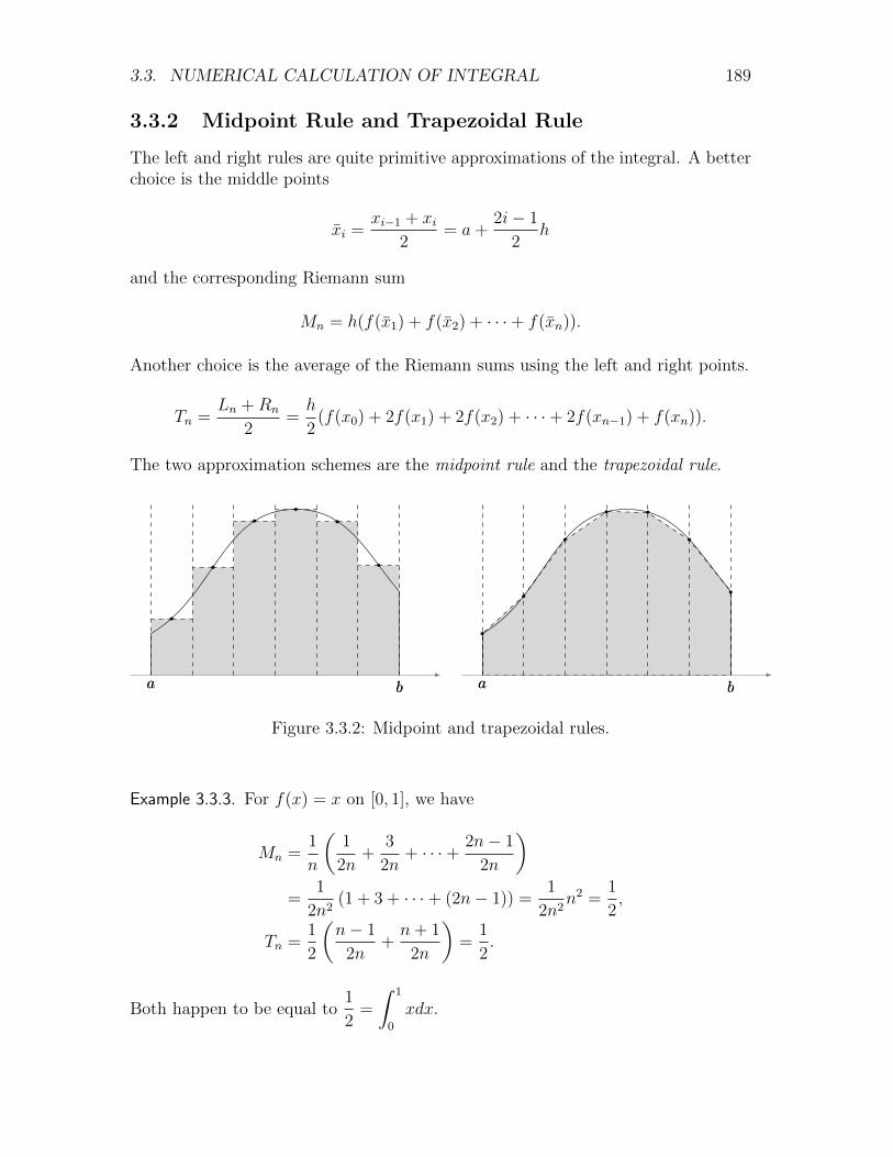
3.3. NUMERICAL CALCULATION OF INTEGRAL 189
3.3.2 Midpoint Rule and Trapezoidal Rule
The left and right rules are quite primitive approximations of the integral. A betterchoice is the middle points
xi =xi−1 + xi
2= a+
2i− 1
2h
and the corresponding Riemann sum
Mn = h(f(x1) + f(x2) + · · ·+ f(xn)).
Another choice is the average of the Riemann sums using the left and right points.
Tn =Ln +Rn
2=h
2(f(x0) + 2f(x1) + 2f(x2) + · · ·+ 2f(xn−1) + f(xn)).
The two approximation schemes are the midpoint rule and the trapezoidal rule.
a b a ba b a b
Figure 3.3.2: Midpoint and trapezoidal rules.
Example 3.3.3. For f(x) = x on [0, 1], we have
Mn =1
n
(1
2n+
3
2n+ · · ·+ 2n− 1
2n
)=
1
2n2(1 + 3 + · · ·+ (2n− 1)) =
1
2n2n2 =
1
2,
Tn =1
2
(n− 1
2n+n+ 1
2n
)=
1
2.
Both happen to be equal to1
2=
∫ 1
0
xdx.

190 CHAPTER 3. INTEGRATION
Example 3.3.4. For f(x) = x2 on [0, 1], we have
Mn =1
n
(12
4n2+
32
4n2+ · · ·+ (2n− 1)2
4n2
)=
1
4n3[(12 + 22 + · · ·+ (2n)2)− 22(12 + 23 + · · ·+ n2)]
=1
4n3
(1
62n(2n+ 1)(4n+ 1)− 1
6n(n+ 1)(2n+ 1)
)=
4n2 − 1
12n2,
Tn =1
2n
(02
n2+ 2
12
n2+ 2
22
n2+ · · ·+ 2
(n− 1)2
n2+n2
n2
)=
1
2n3[2(12 + 22 + · · ·+ n2)− n2]
=1
2n3
(2
1
6n(n+ 1)(2n+ 1)− n2
)=
2n2 + 1
6n2.
Compared with the actual value
∫ 1
0
x2dx =1
3, the errors are
1
12n2and
1
6n2.
Example 3.3.5. We apply the midpoint and trapezoidal rules to
∫ 1
0
dx
1 + x2. For
n = 4, we have
M4 = 0.25× (0.984615 + 0.876712 + 0.719101 + 0.566372) ≈ 0.786700,
T4 =0.25
2× (1.000000 + 2× 0.941176 + 2× 0.800000 + 2× 0.640000 + 0.500000)
≈ 0.782794.
For n = 8, we have h = 0.125 and the following values.
i xi1
1 + x2i
xi1
1 + x2i
0 0 1.0000001 0.125 0.984615 0.0625 0.9961092 0.25 0.941176 0.1875 0.9660383 0.325 0.876712 0.3125 0.9110324 0.5 0.800000 0.4375 0.8393445 0.625 0.719101 0.5625 0.7596446 0.75 0.640000 0.6875 0.6790457 0.875 0.566372 0.8125 0.6023538 1 0.500000 0.9375 0.532225
Then we get the approximations
M8 ≈ 0.785721, T8 ≈ 0.784747.
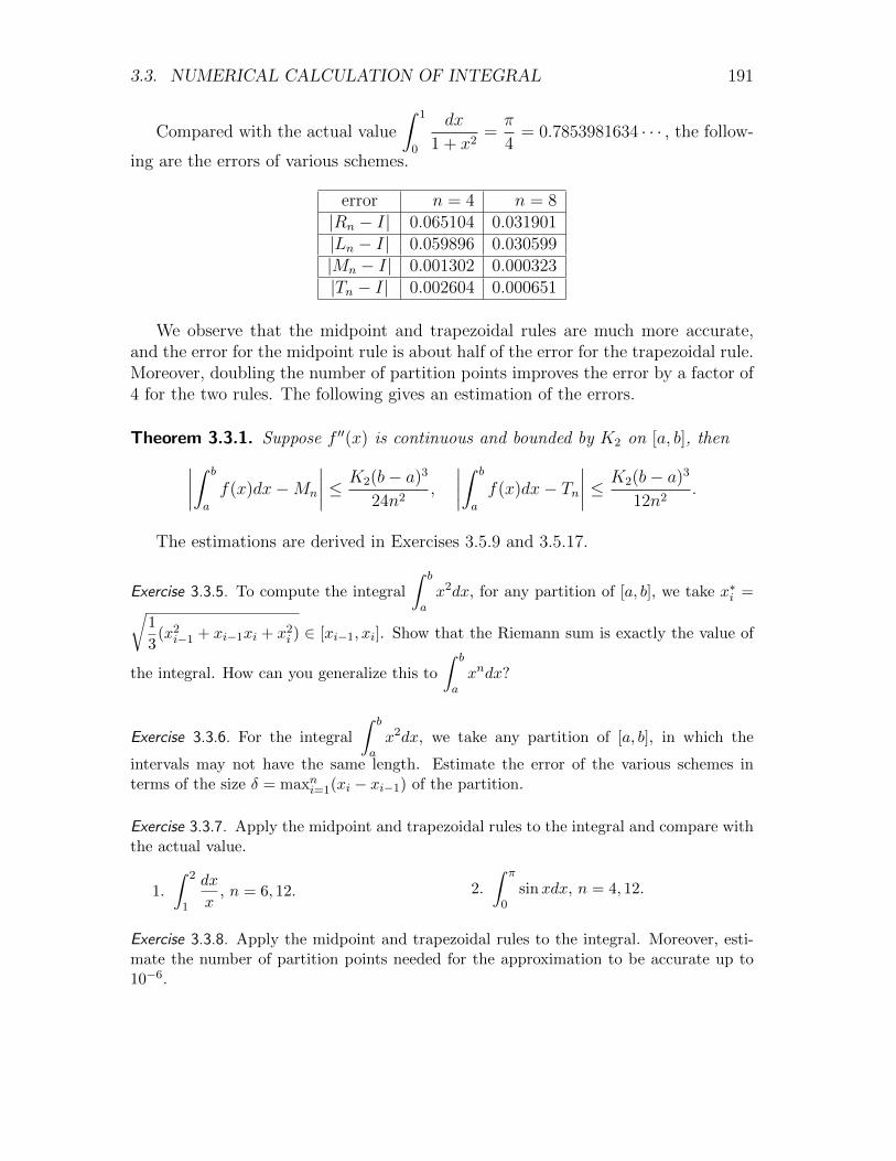
3.3. NUMERICAL CALCULATION OF INTEGRAL 191
Compared with the actual value
∫ 1
0
dx
1 + x2=π
4= 0.7853981634 · · · , the follow-
ing are the errors of various schemes.
error n = 4 n = 8|Rn − I| 0.065104 0.031901|Ln − I| 0.059896 0.030599|Mn − I| 0.001302 0.000323|Tn − I| 0.002604 0.000651
We observe that the midpoint and trapezoidal rules are much more accurate,and the error for the midpoint rule is about half of the error for the trapezoidal rule.Moreover, doubling the number of partition points improves the error by a factor of4 for the two rules. The following gives an estimation of the errors.
Theorem 3.3.1. Suppose f ′′(x) is continuous and bounded by K2 on [a, b], then∣∣∣∣∫ b
a
f(x)dx−Mn
∣∣∣∣ ≤ K2(b− a)3
24n2,
∣∣∣∣∫ b
a
f(x)dx− Tn∣∣∣∣ ≤ K2(b− a)3
12n2.
The estimations are derived in Exercises 3.5.9 and 3.5.17.
Exercise 3.3.5. To compute the integral
∫ b
ax2dx, for any partition of [a, b], we take x∗i =√
1
3(x2i−1 + xi−1xi + x2
i ) ∈ [xi−1, xi]. Show that the Riemann sum is exactly the value of
the integral. How can you generalize this to
∫ b
axndx?
Exercise 3.3.6. For the integral
∫ b
ax2dx, we take any partition of [a, b], in which the
intervals may not have the same length. Estimate the error of the various schemes interms of the size δ = maxni=1(xi − xi−1) of the partition.
Exercise 3.3.7. Apply the midpoint and trapezoidal rules to the integral and compare withthe actual value.
1.
∫ 2
1
dx
x, n = 6, 12. 2.
∫ π
0sinxdx, n = 4, 12.
Exercise 3.3.8. Apply the midpoint and trapezoidal rules to the integral. Moreover, esti-mate the number of partition points needed for the approximation to be accurate up to10−6.

192 CHAPTER 3. INTEGRATION
1.
∫ π
0cosx2dx, n = 5, 10.
2.
∫ π
0
sinx
xdx, n = 5, 10.
3.
∫ 2
0
1√1 + x3
dx, n = 5, 10.
4.
∫ 1
0ex
2dx, n = 10.
5.
∫ 2
1e
1xdx, n = 10.
6.
∫ 2
1
log x
1 + xdx, n = 10.
Exercise 3.3.9. Show that T2n =1
2(Mn + Tn).
Exercise 3.3.10. Prove that if f is a concave positive function, then Tn ≤∫ b
af(x)dx < Mn.
3.3.3 Simpson’s Rule
The midpoint rule is based on the constant approximation, and the trapezoidal ruleis based on linear approximation (actually not quite, as average of two constantapproximations). We may expect better approximation by using quadratic curves.
Since a quadratic curve is determined by three points, we try to approximate f(x)on the interval [xi−1, xi+1] by the quadratic function Q(x) = A(x−xi)2+B(x−xi)+Csatisfying
f(xi−1) = Q(xi−1) = Ah2 −Bh+ C,
f(xi) = Q(xi) = C,
f(xi+1) = Q(xi+1) = Ah2 +Bh+ C.
Then
∫ xi+1
xi−1
f(x)dx is approximated by (the first equality uses (3.1.6))
∫ xi+1
xi−1
Q(x)dx =2
3Ah3 + 2Ch =
h
3(f(xi−1) + 4f(xi) + f(xi+1)).
Suppose n is even. Then we may apply the quadratic approximations to [x0, x2],[x2, x4], . . ., [xn−2, xn]. Adding such approximations together, we get an approxima-
tion of
∫ b
a
f(x)dx
Sn =h
3(f(x0)+4f(x1)+2f(x2)+4f(x3)+2f(x4)+· · ·+2f(xn−2)+4f(xn−1)+f(xn)).
This is Simpson’s rule. Observe that Sn =1
3(2Tn +Mn
2) is the weighted average of
the trapezoidal (with step size h) and midpoint (with step size 2h) rules.The errors in Simpson’s rule can be estimated by the bound on the fourth order
derivative.

3.3. NUMERICAL CALCULATION OF INTEGRAL 193
Theorem 3.3.2. Suppose f (4)(x) is continuous and bounded by K4 on [a, b], then∣∣∣∣∫ b
a
f(x)dx− Sn∣∣∣∣ ≤ K4(b− a)5
180n4.
A consequence of the theorem is that doubling the partition improves the errorby a factor of 16!
Example 3.3.6. Applying Simpson’s rule to
∫ 1
0
dx
1 + x2for n = 4, we use the same
data from Example 3.3.1 to get
S4 =0.25
3× (1.000000 + 4× 0.941176 + 2× 0.800000 + 4× 0.640000 + 0.500000)
≈ 0.785392.
The error |Sn − I| = 0.000540 is comparable to the midpoint and trepezoidal rulefor n = 8.
How many partition points are needed in order to get the approximate valueaccurate up to the 6-th digit? To answer the question, we compute the derivatives
f (4)(x) =24(5x4 − 10x2 + 1)
(1 + x2)5, f (5)(x) = −240x(x2 − 3)(3x2 − 1)
(1 + x2)6.
From f (5)(x), the extrema of f (4)(x) on [0, 1] can only be at 0,1√3
or 1. By
|f (4)(0)| = 24,
∣∣∣∣f (4)
(1√3
)∣∣∣∣ =81
8, |f (4)(1)| = 3,
we get K4 = 24. Then the question becomes
24
180n4≤ 10−6.
Therefore we need n ≥ 19.1. Since n should be an even integer, this means n ≥ 20.We may carry out the similar estimation for the midpoint and trapezoidal rules.
We find K2 = |f ′′(0)| = 2, so that the estimations become
2
24n2≤ 10−6,
2
12n2≤ 10−6.
The answers are respectively n ≥ 289 and n ≥ 409.
Exercise 3.3.11. Repeat Exercise 3.3.7 for the Simpson’s rule.
Exercise 3.3.12. Repeat Exercise 3.3.8 for the Simpson’s rule.

194 CHAPTER 3. INTEGRATION
Exercise 3.3.13. If we apply Simpson’s rule to
∫ 1
0
dx
1 + x2to get an approximate value for
π accurate up to 10−6, how many partition points do we need?
Exercise 3.3.14. Simpson’s 3/8 rule is obtained by using cubic instead of quadratic approx-imation. Derive the formula for this rule.
3.4 Indefinite Integral
3.4.1 Fundamental Theorem of Calculus
The Newton-Leibniz formula is derived from A′(x) = f(x), where A(x) =
∫ x
a
f(t)dt
is the signed area over [a, x]. The equality is summarized below.
Theorem 3.4.1 (Fundamental Theorem of Calculus). If f(x) is continuous at x, then
d
dx
∫ x
a
f(t)dt = f(x).
Note that the continuity was used critically in our argument for A′(x) = f(x).
Example 3.4.1. Let f(x) be a continuous function. To find the derivative of
∫ x2
a
f(t)dt,
we note that the integral is a composition∫ x2
a
f(t)dt = A(x2), A(x) =
∫ x
a
f(t)dt.
By the chain rule and the Fundamental Theorem of Calculus, we have
d
dx
∫ x2
a
f(t)dt =dA(x2)
dx= A′(x2)2x = 2xf(x2).
The Fundamental Theorem also implies the following derivatives
d
dx
∫ x
a
f(t2)dt = f(x2),
d
dx
∫ x
a
f(t)2dt = f(x)2,
d
dx
(∫ x
a
f(t)dt
)2
= 2f(x)
∫ x
a
f(t)dt.

3.4. INDEFINITE INTEGRAL 195
Example 3.4.2. The function f(x) =
∫ x
0
et2
dt cannot be expressed as combinations
of the usual elementary functions. Still, we know f ′(x) = ex2. We also have
d
dx
∫ x2
x
et2
dt =d
dx
(∫ x2
0
et2
dt−∫ x
0
et2
dt
)= 2xex
4 − ex2
.
Example 3.4.3. For the sign function
sign(x) =
1, if x > 0,
0, if x = 0,
−1, if x < 0,
we have
A(x) =
∫ x
0
sign(x)dx = |x|, A′(x) =
1, if x > 0,
no, if x = 0,
−1, if x < 0.
We note that A(x) is not differentiable at 0, exactly the place where the sign functionis not continuous. The example shows that the continuity assumption cannot bedropped from the Fundamental Theorem.
Example 3.4.4. The sine integral function is
Si(x) =
∫ x
0
sin t
tdt.
Since the integrand can be made continuous by assigning value 1 at 0, we know
Si′(x) =
sinx
x, if x 6= 0,
1, if x = 0.
Therefore the function Si(x) is strictly increasing on the following intervals
. . . , [−5π,−4π], [−3π,−2π], [−π, π], [2π, 3π], [4π, 5π], . . . ,
and is strictly decreasing on the following intervals
. . . , [−4π,−3π], [−2π,−π], [π, 2π], [3π, 4π], . . . .
This implies that Si(x) has local maxima at . . . ,−6π,−4π,−2π, π, 3π, 5π, . . . , andhas local minima at . . . ,−5π,−3π,−π, 2π, 4π, 6π, . . . . Moreover, we can also calcu-late the second order derivative
Si′′(x) =
x cosx− sinx
x2, if x 6= 0,
0, if x = 0,
and find the convexity property of Si(x).

196 CHAPTER 3. INTEGRATION
Example 3.4.5. Suppose f is a continuous function satisfying
2
∫ x
0
tf(t)dt = x
∫ x
0
f(t)dt.
Then by taking derivative on both sides, we get
2xf(x) = xf(x) +
∫ x
0
f(t)dt.
Let F (x) =
∫ x
0
f(t)dt. Then the equation is the same as xF ′(x) = F (x). This
implies (F (x)
x
)′=xF ′(x)− F (x)
x2= 0.
Therefore
∫ x
0
f(t)dt = F (x) = Cx for a constant C, and we further find that
f(x) = C is a constant.
Exercise 3.4.1. Find the derivative of function.
1.
∫ x
0t3dt. 2.
∫ x2
0t3dt. 3.
∫ x3
0t2dt. 4.
∫ x3
x2
t2dt.
Exercise 3.4.2. Find the derivative of function.
1.
∫ x
1
dt
1 + t3.
2.
∫ x2
1log(1 + t2)dt.
3.
∫ π
xcos t2dt.
4.
∫ 1
x2
√1 +√tdt.
5.
∫ π
tanxarctan tdt.
6.
∫ cotx
tanx(1 + t2)
32dt.
Exercise 3.4.3. Let f(x) be a continuous function. Find the derivative.
1.
∫ b
x2
f(t)dt.
2.
∫ x2
xf(t)dt.
3.
∫ x
af(t2)dt.
4.
∫ x
aef(t)dt.
5.
∫ b
xf(sin t)dt.
6.
∫ cosx
sinxf(t)dt.
7.
∫ f(x)
0f(t)dt.
8.
∫ f−1(x)
0f(t)dt.
In the 7-th problem, f is differentiable. In the 8-th problem, f is invertible anddifferentiable.
Exercise 3.4.4. Study the monotone and convex properties, including the extrema and thepoints of inflection.

3.4. INDEFINITE INTEGRAL 197
1.
∫ x
0
dt
1 + t+ t2. 2.
∫ x
0sin
πt2
2dt. 3.
2√π
∫ x
0e−t
2dt.
Exercise 3.4.5. Find continuous functions f(x) satisfying the equality.
1.
∫ x
0f(t)dt =
∫ 1
xf(t)dt on [0, 1].
2. A
∫ x
0tf(t)dt = x
∫ x
0f(t)dt on (0,+∞).
3. (f(x))2 = 2
∫ x
0f(t)dt on (−∞,+∞).
4.
∫ x
0f(t)dt = (2x− 1)e2x +
∫ x
0e−tf(t)dt on (−∞,+∞).
Exercise 3.4.6. Find the limit.
1. limx→01
x
∫ x
0
sin t
tdt.
2. limx→01
x3
∫ x
0sin t2dt.
3. limx→+∞
(∫ x
0et
2dt
)2
∫ x
0e2t2dt
.
Exercise 3.4.7. Prove that for a positive continuous function f(x) on (0,+∞), the function
g(x) =
(∫ x
0tf(t)dt
)2
∫ x
0f(t)dt
is strictly increasing on (0,+∞).
Exercise 3.4.8. Discuss where f(x) is not continuous and where
∫ x
0f(t)dt is not differen-
tiable.
1. f(x) =
{x, if x 6= 0,
1, if x = 0,.
2. f(x) =
{x, if x > 0,
1, if x ≤ 0,.
3. f(x) =
(x2 sin
1
x
)′, if x 6= 0,
0, if x = 0,
.
3.4.2 Indefinite Integral
A function F is an antiderivative of f if F ′ = f . By Theorem 2.4.3, the antiderivativeis unique up to adding constants. Therefore we denote all the antiderivatives of f

198 CHAPTER 3. INTEGRATION
by ∫f(x)dx = F (x) + C, for some F (x) satisfying F ′(x) = f(x).
This is the indefinite integral of f .The Newton-Leibniz formula says that the definite integral of a continuous func-
tion can be calculated from the antiderivative∫ b
a
f(x)dx = F (b)− F (a).
The Fundamental Theorem of Calculus says that the signed area gives one an-tiderivative, and can be used as F (x) above∫
f(x)dx =
∫ x
a
f(t)dt+ C.
Example 3.4.6. By
(xp+1)′ = (p+ 1)xp, (log |x|)′ = 1
x, (ex)′ = ex,
we get ∫xpdx =
xp+1
p+ 1+ C, for p 6= −1,
log |x|+ C, for p = −1;
∫exdx = ex + C.
More generally, we have
∫(ax+ b)pdx
(ax+ b)p+1
(p+ 1)a+ C, for p 6= −1,
1
alog |ax+ b|+ C, for p = −1;
∫axdx =
ax
log a+ C.
Example 3.4.7. The antiderivative of the logarithmic function is more complicated∫log |x|dx = x log |x| − x+ C.
The equality can be verified by taking the derivative
(x log |x| − x)′ = log |x|+ x1
x− 1 = log |x|.
Example 3.5.9 gives the systematic way of deriving
∫log |x|dx.

3.4. INDEFINITE INTEGRAL 199
Example 3.4.8. The derivatives of the trigonometric functions give us∫cosxdx = sinx+ C,
∫sinxdx = − cosx+ C,∫
sec2 xdx = tanx+ C,
∫secx tanxdx = secx+ C.
The antiderivatives of tan x and secx are more complicated, and are given in Ex-ample 3.5.27.
Example 3.4.9. The derivative of the inverse sine function gives∫dx√
1− x2= arcsinx+ C,
∫dx√a2 − x2
= arcsinx
a+ C, a > 0.
Similarly, the derivative of the inverse tangent function gives∫dx
x2 + 1= arctanx+ C,
∫dx
x2 + a2=
1
aarctan
x
a+ C.
The similar integrals
∫dx
x2 − a2and
∫dx√x2 + a
are given in Exercise 3.4.10 and
Examples 3.5.2, 3.5.31, 3.5.32.
Exercise 3.4.9. Compute the integrals.
1.
∫4√
1− xdx.
2.
∫1
3√
2x+ 1dx.
3.
∫axdx.
4.
∫csc2 xdx.
5.
∫cscx cotxdx.
6.
∫dx
cos2 x.
Exercise 3.4.10. Verify the antiderivatives.
1.
∫log |x|x
dx =1
2(log |x|)2 + C.
2.
∫eax cos bxdx =
eax
a2 + b2(a cos bx+ b sin bx) + C.
3.
∫cos(ax+ b)dx =
1
asin(ax+ b) + C.
4.
∫ √a2 − x2dx =
a2
2arcsin
x
a+
1
2x√a2 − x2 + C, a > 0.
5.
∫dx
x2 − a2=
1
2alog
∣∣∣∣x− ax+ a
∣∣∣∣+ C.
6.
∫dx√x2 + a
= log∣∣∣x+
√x2 + a
∣∣∣+ C.

200 CHAPTER 3. INTEGRATION
7.
∫ √x2 + adx =
1
2x√x2 + a+
a
2log∣∣∣x+
√x2 + a
∣∣∣+ C.
Exercise 3.4.11. If
∫f(x)dx = F (x) + C, then what is
∫f(ax + b)dx? Apply your
conclusion to compute the integrals.
1.
∫log |a+ bx|dx.
2.
∫sin(ax+ b)dx.
3.
∫sec2(3x− 1)dx.
4.
∫dx√
1− (x− 1)2.
5.
∫dx√
x(1− x).
6.
∫dx
x2 + 2x+ 2.
Exercise 3.4.12. Find the antiderivative of x(ax2 + b)p. Then compute the integrals.
1.
∫x√x2 + 3dx. 2.
∫xdx
x2 + 1. 3.
∫xdx√4− x2
.
Exercise 3.4.13. Compute the integrals.
1.
∫x sin(ax2 + b)dx. 2.
∫xeax
2+bdx. 3.
∫x2(ax3 + b)pdx.
One should not just mindlessly compute the antiderivative. Sometimes we needto consider the meaning of antiderivative and question whether the answer makessense.
Example 3.4.10. Without much thinking, we may write∫|x|dx =
1
2x2 + C, if x ≥ 0,
−1
2x2 + C, if x < 0.
However, the constant C in the two cases cannot be independently chosen becausethe antiderivative must be differentiable and is therefore continuous at 0. The moresensible answer is ∫
|x|dx =
1
2x2, if x ≥ 0
−1
2x2, if x < 0
+ C.
In other words, the constant C is two cases must be equal.For another example, instead of
f(x) =
{ex, if x ≥ 0,
1, if x < 0,
∫f(x)dx =
{ex + C, if x ≥ 0,
x+ C, if x < 0,
we should have ∫f(x)dx =
{ex, if x ≥ 0
x+ 1, if x < 0+ C.

3.5. PROPERTIES OF INTEGRATION 201
Exercise 3.4.14. Compute indefinite integral.
1.
{x2, if x ≤ 0,
sinx, if x > 0.. 2.
{1− x2, if |x| ≤ 1,
sin(1− |x|), if |x| > 1..
Exercise 3.4.15. Does the sign function
sign(x) =
1, if x > 0,
0, if x = 0,
−1, if x < 0,
have antiderivative? Does the function have definite integral? What do you learn fromthe example?
3.5 Properties of Integration
Computationally, integration is the reverse of differentiation. Therefore propertiesof differentiation have corresponding properties of integration.
3.5.1 Linear Property
Suppose F (x) and G(x) are antiderivatives of f(x) and g(x). Then the linear prop-erty of the derivative
(F (x) +G(x))′ = F ′(x) +G′(x) = f(x) + g(x), (cF (x))′ = cF ′(x) = cf(x),
implies the linear property of the antiderivative∫(f(x) + g(x))dx =
∫f(x)dx+
∫g(x)dx,
∫cf(x)dx = c
∫f(x)dx.
By the Newton-Leibniz formula, we get the linear property for the definite integral∫ b
a
(f(x) + g(x))dx = (F (b) +G(b))− (F (a) +G(a))
= (F (b)− F (a)) + (G(b)−G(a)) =
∫ b
a
f(x)dx+
∫ b
a
g(x)dx,∫ b
a
cf(x)dx = cF (b)− cF (a) = c(F (b)− F (a)) = c
∫ b
a
f(x)dx.
Example 3.5.1. We have∫x(1 + x)2dx =
∫(x+ 2x2 + x3)dx =
∫xdx+ 2
∫x2dx+
∫x3dx
=1
2x2 +
2
3x3 +
1
4x4 + C.

202 CHAPTER 3. INTEGRATION
This furthers gives the definite integral∫ 1
0
x(1 + x)2dx =1
2(12 − 02) +
2
3(13 − 03) +
1
4(14 − 04) =
17
12.
On the other hand, it would be very complicated to compute
∫x(x+ 1)10dx by
the binomial expansion of (1 + x)10. The following is much simpler∫x(x+ 1)10dx =
∫((x+ 1)− 1)(x+ 1)10dx =
∫(x+ 1)11dx−
∫(x+ 1)10dx
=1
12(x+ 1)12 − 1
11(x+ 1)11 + C =
1
12 · 11(11x− 1)(x+ 1)11 + C.
Exercise 3.5.1. Compute the integrals.
1.
∫x√x+ 1dx.
2.
∫x(ax+ b)pdx.
3.
∫x2(ax+ b)pdx.
4.
∫(x− 1)(x+ 1)
43dx.
5.
∫(x− 1)(x+ 1)pdx.
6.
∫x
(x+ 1)10dx.
7.
∫x2 − x+ 1
(x+ 1)10dx.
8.
∫x− 1√xdx.
9.
∫ (x− 1
x
)2
dx.
10.
∫ (x− 1
x2
)2
dx.
11.
∫ (x− 1
x+ 1
)2
dx.
12.
∫(x− 1)2
(x+ 1)4dx.
Exercise 3.5.2. Find A,B satisfying
ax+ b
cx+ d= A+
B
cx+ d.
Then compute the antiderivatives ofax+ b
cx+ dand
(ax+ b
cx+ d
)2
.
Exercise 3.5.3. Compute the integrals.
1.
∫(ex − e−x)2dx. 2.
∫(2x + 3x)2dx. 3.
∫2x+1 − 3x−1
6xdx.
Example 3.5.2. To find the antiderivative of1
x2 − a2, we use
1
x2 − a2=
1
(x− a)(x+ a)=
1
2a
(1
x− a− 1
x+ a
)to get ∫
dx
x2 − a2=
1
2alog |x− a| − 1
2alog |x+ a|+ C =
1
2alog
∣∣∣∣x− ax+ a
∣∣∣∣+ C.

3.5. PROPERTIES OF INTEGRATION 203
This furthers gives the definite integral∫ 3
2
1
x2 − 1dx =
1
2log
∣∣∣∣3− 1
3 + 1
∣∣∣∣− 1
2log
∣∣∣∣2− 1
2 + 1
∣∣∣∣ =1
2log
3
2.
As noted in Example 3.1.4, we should not blindly use the Newton-Leibniz formulain competing the definite integral. For example, we cannot get∫ 2
0
1
x2 − 1dx =
1
2log
∣∣∣∣2− 1
2 + 1
∣∣∣∣− 1
2log
∣∣∣∣0− 1
0 + 1
∣∣∣∣ = −1
2log 3,
because the interval [0, 2] contains 1, where the integrand approaches infinity.
Example 3.5.3. The idea in Example 3.5.2 can be extended∫dx
x(x+ 1)(x+ 2)=
∫1
x
(1
x+ 1− 1
x+ 2
)dx =
∫ (1
x(x+ 1)− 1
x(x+ 2)
)dx
=
∫ [(1
x− 1
x+ 1
)− 1
2
(1
x− 1
x+ 2
)]dx
=1
2log |x| − log |x+ 1|+ 1
2log |x+ 2|+ C
=1
2log
∣∣∣∣x(x+ 2)
(x+ 1)2
∣∣∣∣+ C,∫dx
(x2 − 1)2=
1
4
∫ (1
x− 1− 1
x+ 1
)2
dx
=1
4
∫ (1
(x− 1)2+
1
(x+ 1)2− 2
(x+ 1)(x− 1)
)dx
=1
4
∫ [1
(x− 1)2+
1
(x+ 1)2−(
1
x− 1− 1
x+ 1
)]dx
=1
4
(− 1
x− 1− 1
x+ 1+ log
∣∣∣∣x+ 1
x− 1
∣∣∣∣)+ C
= − x
2(x2 − 1)+
1
4log
∣∣∣∣x+ 1
x− 1
∣∣∣∣+ C.
Exercise 3.5.4. Compute the integrals.
1.
∫xdx
x2 − 1.
2.
∫x2dx
x2 − 1.
3.
∫dx
x2 + 3x+ 2.
4.
∫(2x+ 1)dx
x2 + 3x+ 2.
5.
∫ 1
0
(2x+ 1)dx
x2 + 3x+ 2.
6.
∫x2dx
x2 + 3x+ 2.
7.
∫x2dx
x2 + 1.
8.
∫dx
(x2 + 1)(x2 + 4).
9.
∫x2dx
(x2 + 1)(x2 + 4).

204 CHAPTER 3. INTEGRATION
Exercise 3.5.5. Compute the integrals.
1.
∫dx
(x+ a)(x+ b). 2.
∫xdx
(x+ a)(x+ b). 3.
∫dx
(x+ a)(x+ b)(x+ c).
Example 3.5.4. By trigonometric formula, we have∫ π
0
sin2 xdx =
∫ π
0
1
2(1− cos 2x)dx =
1
2
∫ π
0
xdx− 1
2
∫ π
0
cos 2xdx
=1
4(π2 − 02)− 1
4(sin 2π − sin 0) =
1
4π2.
Similar idea gives∫sin2 xdx =
1
2
∫(1− cos 2x)dx =
1
2x− 1
4sin 2x+ C,∫
sinx cos 2xdx =1
2
∫(sin 3x− sinx)dx = −1
6cos 3x+
1
2cosx+ C,∫
tan2 xdx =
∫(sec2 x− 1)dx = tanx− x+ C.
Exercise 3.5.6. Compute the integrals.
1.
∫cosx sinxdx.
2.
∫ π
0sin2 x cosxdx.
3.
∫cos2 xdx.
4.
∫sin3 xdx.
5.
∫cosx sin 2xdx.
6.
∫cot2 xdx.
7.
∫ π2
0sinx cos 2xdx.
8.
∫ π
0| sinx cos 2x|dx.
9.
∫ π
0| sinx− cosx|dx.
Example 3.5.5. For f ≥ g and a ≤ b, by the inequality (3.1.5) and the linearity ofdefinite integral, we have∫ b
a
f(x)dx−∫ b
a
g(x)dx =
∫ b
a
(f(x)− g(x))dx ≥ 0.
Therefore we have
f ≥ g =⇒∫ b
a
f(x)dx ≥∫ b
a
g(x)dx, for a < b.
The inequality corresponds to Theorem 2.3.3 that uses the derivatives to comparefunctions. However, it is more direct to get the inequality by using the non-negativityof area.
If we apply the inequality to −|f | ≤ f ≤ |f |, then we get∫ b
a
|f(x)|dx ≥∣∣∣∣∫ b
a
f(x)dx
∣∣∣∣ , for a < b.

3.5. PROPERTIES OF INTEGRATION 205
Example 3.5.6 (Average). The average of a function f on [a, b] is1
b− a
∫ b
a
f(x)dx.
If m ≤ f ≤M on [a, b], then
m(b− a) =
∫ b
a
mdx ≤∫ b
a
f(x)dx ≤∫ b
a
Mdx = M(b− a).
This implies that the average of f lies between m and M , which is consistent withour intuition.
For continuous f , we may take m and M to be the minimum and maximum off on [a, b]. By the Intermediate Value Theorem, any value between m and M canbe reached by the function. Therefore the average
1
b− a
∫ b
a
f(x)dx = f(c), for some c ∈ (a, b).
This conclusion is the Integral Mean Value Theorem.
Example 3.5.7. Consider the function F (x) =
∫ x
0
sin t2
tdt. The 4-th order Taylor
expansion T (x) = x − x3
6of sin x means that, for any ε > 0, there is δ > 0, such
that|x| < δ =⇒ | sinx− T (x)| ≤ ε|x|4.
Then for t between 0 and x, we have
|x| <√δ =⇒ |t2| < δ =⇒ | sin t2 − T (t2)| ≤ ε|t|8,
so that
|x| <√δ =⇒
∣∣∣∣sin t2t − t− t5
6
∣∣∣∣ =
∣∣∣∣sin t2t − 1
tT (t2)
∣∣∣∣ ≤ ε|t|7.
Therefore
|x| <√δ =⇒
∣∣∣∣F (x)− x2
2− x6
36
∣∣∣∣ =
∣∣∣∣∫ x
0
(sin t2
t− t− t5
6
)dt
∣∣∣∣ ≤ ε
∫ x
0
|t|7dt =ε
8|x|8.
This means exactly the 7-th order approximation of F (x)
F (x) =1
2x2 +
1
36x6 + o(x8).
Example 3.5.8. Suppose f(x) has second order derivative on [a, b]. We may take the
linear approximation at the middle point c =a+ b
2. By the Lagrange form of the
remainder (Theorem 2.7.1), we get
f(x) = f(c) + f ′(c)(x− c) +f ′′(x)
2(x− c)2,

206 CHAPTER 3. INTEGRATION
where x depends on x and lies between x and c. Then we have∣∣∣∣∫ b
a
(f(x)− f(c)− f ′(c)(x− c))dx∣∣∣∣ =
∣∣∣∣∫ b
a
f ′′(x)
2(x− c)2dx
∣∣∣∣By the linear property of the integral, we have the left side∫ b
a
(f(x)− f(c)− f ′(c)(x− c))dx =
∫ b
a
f(x)dx− f(c)
∫ b
a
dx− f ′(c)∫ b
a
(x− c)dx
=
∫ b
a
f(x)dx− f(c)(b− a).
Let K2 be the bound for the second order derivative. In other words, |f ′′| ≤ K2 on[a, b]. Then the right side∣∣∣∣∫ b
a
f ′′(x)
2(x− c)2dx
∣∣∣∣ ≤ ∫ b
a
|f ′′(x)|2
(x− c)2dx ≤ K2
2
∫ b
a
(x− c)2dx =K2
24(b− a)3.
We conclude the inequality∣∣∣∣∫ b
a
f(x)dx− f(c)(b− a)
∣∣∣∣ ≤ K2
24(b− a)3.
Exercise 3.5.7. Show that the integration of n-th order approximation is (n + 1)-st orderapproximation. Specifically, find high order approximation of function at 0.
1.
∫ x
0
cos t− 1
tdt, order 5.
2.
∫ √x0
sin t− tt2
dt, order 4.
3.
∫ 0
−x2
et − 1
tdt, order 5.
4.
∫ x
−x
log(1 + t)
tdt, order 7.
Exercise 3.5.8. Derive an estimation for
∣∣∣∣∫ b
af(x)dx− f(a)(b− a)
∣∣∣∣ in terms of the bound
K1 of f on [a, b].
Exercise 3.5.9. Apply the estimation in Example 3.5.8 to each interval of a partition andderive the error formula for the midpoint rule in Theorem 3.3.1.
3.5.2 Integration by Parts
The Leibniz rule says that, if F (x) and G(x) are antiderivatives of f(x) and g(x),then
(F (x)G(x))′ = F ′(x)G(x) + F (x)G′(x) = f(x)G(x) + F (x)g(x).

3.5. PROPERTIES OF INTEGRATION 207
In other words, F (x)G(x) is an antiderivative of f(x)G(x) + F (x)g(x), or
F (x)G(x) + C =
∫f(x)G(x)dx+
∫F (x)g(x)dx.
If we use the differential notation
dF (x) = F ′(x)dx = f(x)dx, dG(x) = G′(x)dx = g(x)dx,
then the equality becomes∫F (x)dG(x) = F (x)G(x)−
∫G(x)dF (x).
The equality can be used in the following way. To compute an integral
∫h(x)dx,
we separate the integrand into a product h(x) = F (x)g(x) of two parts and integrate
the second part to get
∫g(x)dx = G(x) + C. Then
∫h(x)dx =
∫F (x)dG(x),
which by the equality above is converted into the computation of another integral∫G(x)dF (x) that exchanges F (x) andG(x). This method of computing the integral
is called the integration by parts.By Newton-Leibniz formula, the integration by parts for indefinite integral im-
plies the method for definite integral∫ b
a
F (x)dG(x) = F (b)G(b)− F (a)G(a)−∫ b
a
G(x)dF (x).
The use of Newton-Leibniz formula requires that f = F ′ and g = G′ to be con-tinuous. Then it is not hard to extend the equality to the case that F and G arecontinuous on [a, b] and have continuous derivatives at all but finitely many pointson [a, b].
Example 3.5.9. The antiderivative of the logarithmic function in Example 3.4.7 maybe derived by using the integration by parts (taking F (x) = log |x| and G(x) = x)∫
log |x|dx = x log |x| −∫xd log |x| = x log |x| −
∫x(log |x|)′dx
= x log |x| −∫dx = x log |x| − x+ C.
The antiderivative x log |x| − x just obtained can be further used∫x log |x|dx =
∫xd(x log |x| − x) = x(x log |x| − x)−
∫(x log |x| − x)dx
= x2 log x− x2 −∫x log |x|dx+
1
2x2.

208 CHAPTER 3. INTEGRATION
Solving the equation, we get∫x log |x|dx =
1
2x2 log x− 1
4x2 + C.
The following is an alternative way of applying the integration by parts to the sameintegral ∫
x log |x|dx =1
2
∫log |x|d(x2) =
1
2x2 − 1
2
∫x2d(log |x|)
=1
2x2 log |x| − 1
2
∫x2 1
xdx =
1
2x2 log |x| − 1
4x2 + C.
We may compute
∫xp log xdx by the similar idea.
Example 3.5.10. The integral in Example 3.5.1 can also be computed by using theintegration by parts∫
x(x+ 1)10dx =1
11
∫xd(x+ 1)11 (integrate (x+ 1)10 part)
=1
11x(x+ 1)11 − 1
11
∫(x+ 1)11dx (exchange two parts)
=1
11x(x+ 1)11 − 1
12 · 11(x+ 1)12 + C.
Example 3.5.11. Using integration by parts, we have∫x2e−xdx = −
∫x2de−x = −x2e−x + 2
∫xe−xdx
= −x2e−x − 2
∫xde−x = −x2e−x − 2xe−x + 2
∫e−xdx
= −(x2 + 2x+ 2)e−x + C.
In general, we have the recursive formula∫xnaxdx =
1
log axnax − n
log a
∫xn−1axdx.
Exercise 3.5.10. Compute the integral.
1.
∫x(ax+ b)pdx. 2.
∫x2(ax+ b)pdx. 3.
∫(x− 1)(x+ 1)pdx.
Exercise 3.5.11. Compute the integral.

3.5. PROPERTIES OF INTEGRATION 209
1.
∫(x2 − 1)axdx. 2.
∫(x+ ax)2dx. 3.
∫xexdx
(x+ 1)2.
Exercise 3.5.12. Compute the integral.
1.
∫x2 log |x|dx.
2.
∫xp log xdx.
3.
∫(log |x|)2dx.
4.
∫xp(log |x|)2dx.
5.
∫x log(x+ 1)dx.
6.
∫x log
1 + x
1− xdx.
Exercise 3.5.13. Derive the recursive formula for
∫(log |x|)ndx. How about
∫xp(log x)ndx?
Exercise 3.5.14. Compute
∫ 1
0xnaxdx.
Exercise 3.5.15. For natural numbers m,n, show that
∫ 1
0xm(1− x)ndx =
m!n!
(m+ n+ 1)!.
Exercise 3.5.16. Compute the integral.
1.
∫log(√x+ a+
√x− a)dx.
2.
∫log(√a+ x−
√a− x)dx.
3.
∫ (log(x+ a)
x+ b+
log(x+ b)
x+ a
)dx.
4.
∫x√
1 + x2log(x+
√1 + x2)dx.
5.
∫x log(x+
√1 + x2)√
1 + x2dx.
6.
∫ (log(x+
√1 + x2)
)2dx.
Exercise 3.5.17. Let f have second order derivative on [a, b].
1. Show that for any constants A and B, we have∫ b
af(x)dx =
((x+A)f(x)− 1
2((x+A)2 +B)f ′(x)
)ba
+1
2
∫ b
a((x+A)2 +B)f ′′(x)dx.
2. By choosing suitable A and B in the first part, show that∫ b
af(x)dx =
f(a) + f(b)
2(b− a) +
∫ b
a((x+A)2 + 2B)f ′′(x)dx,
and ∫ b
a|(x+A)2 + 2B|dx =
1
12(b− a)3.
3. Use the second part to derive the error formula for the trapezoidal rule in Theorem3.3.1.

210 CHAPTER 3. INTEGRATION
Example 3.5.12. Using the integration by parts, we have∫x cosxdx =
∫xd sinx = x sinx−
∫sinxdx = x sinx+ cosx+ C.
The idea can be extended to product of xn, sin ax and cos bx for various a and b∫x sinx sin 2xdx =
1
2
∫x(cos 3x− cosx)dx =
1
2
∫xd
(1
3sin 3x− sinx
)=
1
6x(sin 3x− 3 sinx)− 1
6
∫(sin 3x− 3 sinx)dx
=1
6x sin 3x− 1
2x sinx+
1
18cos 3x− 1
2cosx+ C.
An example of the definite integral is∫ π2
0
x2 sinxdx = −∫ π
2
0
x2d cosx = −(π
2
)2
cosπ
2+ 02 cos 0 +
∫ π2
0
2x cosxdx
= 2
∫ π2
0
xd sinx = 2π
2sin
π
2− 2 · 0 sin 0− 2
∫ π2
0
sinxdx
= π + 2 cosπ
2− 2 cos 0 = π − 2.
Example 3.5.13. Let
I0 =
∫eax cos bxdx, J0 =
∫eax sin bxdx.
We have
I0 = a−1
∫cos bxdeax = a−1eax cos bx− a−1
∫eaxd cos bx
= a−1eax cos bx+ a−1bJ0,
J0 = a−1
∫sin bxdeax = a−1eax sin bx− a−1
∫eaxd sin bx
= a−1eax sin bx− a−1bI0.
Solving the system for I0 and J0, we get∫eax cos bxdx =
eax
a2 + b2(a cos bx+ b sin bx) + C,∫
eax sin bxdx =eax
a2 + b2(−b cos bx+ a sin bx) + C.
Let
I1 =
∫xex cosxdx, J1 =
∫xex sinxdx.

3.5. PROPERTIES OF INTEGRATION 211
Using the earlier computation of I0 and J0, we have
I1 =
∫x cosxdex = xex cosx−
∫(cosx− x sinx)exdx
= xex cosx− 1
2ex(cosx+ sinx) + J1.
Similarly, we have
J1 = xex sinx− 1
2ex(− cosx+ sinx)− I1.
Solving the two equations, we get∫xex cosxdx =
1
2xex(cosx+ sinx)− ex sinx+ C,∫
xex sinxdx =1
2xex(− cosx+ sinx) + ex cosx+ C.
Example 3.5.14. Let
Im,n =
∫cosm x sinn xdx.
If n 6= 0, then we may integrate a copy of sin x to get
Im,n = −∫
cosm x sinn−1 xd cosx
= − cosm+1 x sinn−1 x
+
∫(−m cosm−1 x sinn x+ (n− 1) cosm+1 x sinn−2 x) cosxdx
= − cosm+1 x sinn−1 x
+
∫(−m cosm x sinn x+ (n− 1) cosm x(1− sin2 x) sinn−2 x)dx
= − cosm+1 x sinn−1 x− (m+ n− 1)Im,n − (n− 1)Im,n−2.
Therefore (the formula can be directly verified for n = 0)
Im,n = − 1
m+ ncosm+1 x sinn−1 x+
n− 1
m+ nIm,n−2, m+ n 6= 0.
The formula reduces the power of sine by 2. If we first integrate a copy of cosx,then we get another recursive relation that reduces the power of cosine by 2
Im,n =1
m+ ncosm−1 x sinn+1 x+
m− 1
m+ nIm−2,n, m+ n 6= 0.

212 CHAPTER 3. INTEGRATION
On the other hand, we can also express Im,n−2 and Im−2,n in terms of Im,n. Aftersubstituting n by n+ 2, we get recursive relations that increase the power by 2
Im,n =1
n+ 1cosm+1 x sinn+1 x+
m+ n+ 2
n+ 1Im,n+2, n 6= −1,
= − 1
m+ 1cosm+1 x sinn+1 x+
m+ n+ 2
m+ 1Im+2,n, m 6= −1.
Here is a concrete example of using the recursive relation∫cos4 x sin6 xdx = I4,6 = − 1
4 + 6cos4+1 x sin6−1 x+
6− 1
4 + 6I4,6−2
= − 1
10cos5 x sin5 x+
5
10I4,4
= − 1
10cos5 x sin5 x+
5
10
(−1
8cos5 x sin3 x+
3
8I4,2
)= − cos5 x
(1
10sin5 x+
5
10 · 8sin3 x
)+
5 · 310 · 8
(−1
6cos5 x sinx+
1
6I4,0
)= − cos5 x
(1
10sin5 x+
5
10 · 8sin3 x+
5 · 310 · 8 · 6
sinx
)+
5 · 3 · 110 · 8 · 6
(1
4cos3 x sinx+
3
4I2,0
)= − cos5 x
(1
10sin5 x+
5
10 · 8sin3 x+
5 · 310 · 8 · 6
sinx
)+
5 · 3 · 110 · 8 · 6
1
4cos3 x sinx+ +
5 · 3 · 110 · 8 · 6
3
4
(1
2cosx sinx+
1
2I0,0
)= − cos5 x
(1
10sin5 x+
5
10 · 8sin3 x+
5 · 310 · 8 · 6
sinx
)+
5 · 3 · 110 · 8 · 6
(1
4cos3 x+
3 · 14 · 2
cosx
)sinx+ +
5 · 3 · 110 · 8 · 6
3 · 14 · 2
x+ C.
Here is another example that requires increasing the power∫sin2 x
cos4 xdx = I−4,2 = − 1
−4 + 1cos−4+1 x sin2+1 x+
−4 + 2 + 2
−4 + 1I−4+2,2
=1
3
sin3 x
cos3 x+ C.
Applying the recursive relation to the definite integral, we have∫ π2
0
sinn xdx = − 1
ncosx sinn−1 x
∣∣∣∣π20
+n− 1
n
∫ π2
0
sinn−2 xdx =n− 1
n
∫ π2
0
sinn−2 xdx.

3.5. PROPERTIES OF INTEGRATION 213
Then we get
∫ π2
0
sinn xdx =n− 1
n
n− 3
n− 2· · ·∫ π
2
0
sin0 or 1 xdx =
(n− 1)!!
n!!
π
2, if n is even,
(n− 1)!!
n!!, if n is odd.
Here sin0 or 1 x takes power 0 for even n and takes power 1 for odd n. Moreover, weused the double factorial
n!! = n(n− 2)(n− 4) · · · =
{2k(2k − 2)(2k − 4) · · · 4 · 2, if n = 2k,
(2k + 1)(2k − 1)(2k − 3) · · · 3 · 1, if n = 2k + 1.
Exercise 3.5.18. Find the recursive relations for
∫xp cos axdx and
∫xp sin axdx. Then
compute the integral.
1.
∫x cos2 xdx.
2.
∫x3 cos2 xdx.
3.
∫x cos2 x sin 2xdx.
4.
∫x3 cos2 x sin 2xdx.
5.
∫ π
0x6 cosxdx.
6.
∫ π2
0x5 sin 2xdx.
Exercise 3.5.19. Find the recursive relations for
∫xpeax cos bxdx and
∫xpeax sin bxdx.
Then compute the integral.
1.
∫x2e−x sin 3xdx. 2.
∫x22x cosxdx. 3.
∫x3ex cos2 xdx.
Exercise 3.5.20. Compute the integral.
1.
∫sin6 xdx.
2.
∫cos8 xdx.
3.
∫cos8 x sin6 xdx.
4.
∫cos3 x sin2 xdx.
5.
∫cos3 x sin5 xdx.
6.
∫cos−2 x sin2 xdx.
7.
∫dx
cos6 x.
8.
∫dx
sin2 x cos2 x.
Exercise 3.5.21. Show that
∫ π2
0sin2m x cos2n xdx =
(2m)!(2n)!
22m+2n+1m!n!(m+ n)!for natural
numbers m,n. Can you find
∫ π2
0sinm x cosn xdx?
Exercise 3.5.22. Use (tanx)′ = sec2 x = tan2 x + 1 to derive the recursive formula for∫secm x tann xdx similar to Example 3.5.14 and then find the value of
∫ π4
0tan2n xdx.

214 CHAPTER 3. INTEGRATION
Example 3.5.15. Let
Ip =
∫(ax2 + bx+ c)pdx, a 6= 0, b2 6= 4ac.
We have
Ip = x(ax2 + bx+ c)p −∫xd(ax2 + bx+ c)p
= x(ax2 + bx+ c)p −∫px(2ax+ b)(ax2 + bx+ c)p−1dx.
We try to express px(2ax+ b) as a combination of (ax2 + bx+ c) and (ax2 + bx+ c)′,up to adding a constant
2pax2 + pbx = A(ax2 + bx+ c) +B(ax2 + bx+ c)′ + C.
We get A = 2p, B = − pb2a
, C =p(b2 − 4ac)
2a. Then
Ip = x(ax2 + bx+ c)p − A∫
(ax2 + bx+ c)pdx
−B∫
(ax2 + bx+ c)p−1(ax2 + bx+ c)′dx− C∫
(ax2 + bx+ c)p−1dx
= x(ax2 + bx+ c)p − AIp −B
p(ax2 + bx+ c)p − CIp−1.
This gives us the recursive relation
Ip =1
(2p+ 1)2a(2ax+ b)(ax2 + bx+ c)p − p(b2 − 4ac)
(2p+ 1)2aIp−1, p 6= −1
2.
On the other hand, we may also express Ip−1 in terms of Ip. After substituting p byp+ 1, we get
Ip =1
(p+ 1)(b2 − 4ac)(2ax+ b)(ax2 + bx+ c)p+1− (2p+ 3)2a
(p+ 1)(b2 − 4ac)Ip+1, p 6= −1.
For the special case
Ip =
∫(ax2 + b)pdx, a, b 6= 0,
the recursive relations become
Ip =1
2p+ 1x(ax2 + b)p +
2pb
2p+ 1Ip−1, p 6= −1
2;
Ip = − 1
2(p+ 1)bx(ax2 + b)p+1 +
2p+ 3
2(p+ 1)bIp+1, p 6= −1.

3.5. PROPERTIES OF INTEGRATION 215
For the special cases of p = −1
2,−1, Ip is given by Exercise 3.4.10 (and will be
derived in Examples 3.5.30, 3.5.31, 3.5.32)∫dx√a2 − x2
= arcsinx
a+ C, a > 0,∫
dx√x2 + a
= log∣∣∣x+
√x2 + a
∣∣∣+ C,∫dx
x2 − a2=
1
2alog
∣∣∣∣x− ax+ a
∣∣∣∣+ C,∫dx
x2 + a2=
1
aarctan
x
a+ C.
Then the recursive relations can be used to compute Ip when p is an integer or ahalf integer. For example, we have∫ √
a2 − x2dx = I 12
=1
2 · 12
+ 1x(a2 − x2)
12 +
2 · 12a2
2 · 12
+ 1I 1
2−1
=1
2x√a2 − x2 +
a2
2arcsin
x
a+ C,∫
(a2 − x2)32dx = I 3
2=
1
2 · 32
+ 1x(a2 − x2)
32 +
2 · 32a2
2 · 32
+ 1I 3
2−1
=1
4x(a2 − x2)
32 +
3a2
4
(1
2x√a2 − x2 +
a2
2arcsin
x
a
)+ C
= −1
8x(2x2 − 5a2)
√a2 − x2 +
3a4
8arcsin
x
a+ C,∫
dx
(x2 + a2)2= I−2 = − 1
2(−2 + 1)a2x(x2 + a2)−2+1 +
2(−2) + 3
2(−2 + 1)a2I−2+1
=x
2a2(x2 + a2)+
1
2a3arctan
x
a+ C.
Exercise 3.5.23. Compute the integral.
1.
∫x2√a2 − x2dx.
2.
∫x√a2 − x2dx.
3.
∫(x+b)2
√a2 − x2dx.
4.
∫x2dx√a2 − x2
.
5.
∫dx
(a2 − x2)32
.
6.
∫xdx
(a2 − x2)32
.
7.
∫dx
(a2 − x2)52
.
8.
∫dx
(a2 − x2)3.
9.
∫xdx
(a2 − x2)3.
Exercise 3.5.24. Compute the integral.

216 CHAPTER 3. INTEGRATION
1.
∫x2√x2 + adx.
2.
∫x√x2 + adx.
3.
∫x2dx√x2 + a
.
4.
∫xdx√x2 + a
.
5.
∫(x2 + a)
32dx.
6.
∫dx
(x2 + a)32
.
7.
∫dx
(x2 + a2)3.
8.
∫xdx
(x2 + a2)3.
9.
∫x2dx
(x2 + a2)3.
Exercise 3.5.25. Combine the ideas of Exercise 3.4.11 and Example 3.5.15 to compute theintegral.
1.
∫dx
(x2 + 2x+ 2)2.
2.
∫dx√
x2 + 2x+ 2.
3.
∫dx
(x2 + 2x+ 2)32
.
4.
∫(x2 + 2x+ 2)
32dx.
5.
∫ √x(1− x)dx.
6.
∫dx
(x(1− x))32
.
3.5.3 Change of Variable
The chain rule says that, if
∫f(y)dy = F (y) + C is the indefinite integral of f(y),
and φ(x) is a differentiable function, then
F (φ(x))′ = F ′(φ(x))φ′(x) = f(φ(x))φ′(x).
In other words, F (φ(x)) is the antiderivative of f(φ(x))φ′(x), or∫f(φ(x))φ′(x)dx = F (φ(x)) + C =
∫f(y)dy
∣∣∣∣y=φ(x)
.
If we use the differential notation dφ(x) = φ′(x)dx, then the equality becomes∫f(φ(x))dφ(x) =
∫f(y)dy
∣∣∣∣y=φ(x)
.
The right side means computing the antiderivative of the function of y first, andthen substituting y = φ(x) into the antiderivative. This is the change of variableformula. By Newton-Leibniz formula, we further get the change of variable formulafor definite integral∫ b
a
f(φ(x))φ′(x)dx =
∫ b
a
f(φ(x))dφ(x) =
∫ φ(b)
φ(a)
f(y)dy.
Example 3.5.16. If
∫f(y)dy = F (y) + C, then by letting y = ax+ b, we have∫
f(ax+ b)dx =1
a
∫f(ax+ b)d(ax+ b) =
1
aF (ax+ b) + C.

3.5. PROPERTIES OF INTEGRATION 217
For example,∫(2x+ 1)pdx =y=2x+1
1
2
∫ypdy =
yp+1
2(p+ 1)+ C =
(2x+ 1)p+1
2(p+ 1)+ C,∫
sin(3x− 2)dx =y=3x−21
3
∫sin ydy = −1
3cos y + C = −1
3cos(3x− 2) + C,∫
dx
x2 + 2x+ 2=
∫dx
(x+ 1)2 + 1=y=x+1
∫dx
y2 + 1
= arctan y + C = arctan(x+ 1) + C.
Example 3.5.17. The following is a simple change of variable∫xex
2
dx =y=x2
1
2
∫eydy =
1
2ey + C =
1
2ex
2
+ C.
The idea is a “mini-integration” of xdx that can be expressed more clearly by writing∫xex
2
dx =
∫ex
2 1
2d(x2) =
1
2ex
2
+ C.
After the mini-integration, we view x2 as the new variable.
The following are more examples following the mini-integration idea∫dx
x log x=
∫1
log x
(dx
x
)=
∫1
log xd(log x) = log | log x|+ C,∫
dx
x2 + a2=
∫d
a2((
xa
)2+ 1) =
∫d(xa
)a((
xa
)2+ 1) =
1
aarctan
x
a+ C,
∫xdx
x4 + a4=
1
2
∫d(x2)
(x2)2 + a4=
1
2a2arctan
x2
a2+ C.
Example 3.5.18. The integral in Example 3.5.1 was computed in Example 3.5.10again by using the integration by parts. The integral can also be computed bychange of variable.
Let y = x+ 1. Then∫x(x+ 1)10dx =
∫(y − 1)y10dy =
∫(y10 − y11)dy =
1
11y11 − 1
12y12 + C.
Substituting y = x+ 1 back, we get∫x(x+ 1)10dx =
1
11(x+ 1)11 − 1
12(x+ 1)12 + C.

218 CHAPTER 3. INTEGRATION
By the same change, we have∫ (x− 1
x+ 1
)4
dx =y=x+1
∫(y − 2)4
y4dy
=
∫(1− 4 · 2y−1 + 6 · 22y−2 − 4 · 23y−3 + 24y−4)dy
= x+ 1− 8 log |x+ 1|
− 24(x+ 1)−1 + 16(x+ 1)−2 − 16
3(x+ 1)−3 + C
= x− 8(9x2 + 12x+ 5)
3(x+ 1)3− 8 log |x+ 1|+ C.
Note that the second C is the first C plus 1.Compare the above with the computation of definite integral∫ 1
0
(x− 1
x+ 1
)4
dx =y=x+1
∫ 2
1
(y − 2)4
y4dy
=
∫ 2
1
(1− 4 · 2y−1 + 6 · 22y−2 − 4 · 23y−3 + 24y−4)dy
=
(y − 8 log y − 24y−1 + 16y−2 − 16
3y−3
)2
1
= 1− 8 log 2− 24
(1
2− 1
)+ 16
(1
4− 1
)− 16
3
(1
8− 1
)=
17
3− 8 log 2.
Note that the evaluation is done by using the new variable y instead of the old x.
Example 3.5.19. The integrals of inverse trigonometric functions can also be com-puted by combining integration by parts and change of variable∫
arcsinxdx = x arcsinx−∫
xdx√1− x2
= x arcsinx+1
2
∫d(1− x2)√
1− x2
= x arcsinx+√
1− x2 + C.
Alternatively, we may simply introduce the trigonometric function as the new vari-able. For example, by y = arcsinx, x = sin y, we have∫
arcsinxdx =
∫yd(sin y) = y sin y −
∫sin ydy
= y sin y + cos y + C = x arcsinx+√
1− x2 + C.
Note that cos y =√
1− x2 is non-negative because x ∈ [−1, 1] and y ∈ [−π2, π
2]. The
integration by parts used in both computations are essentially the same.

3.5. PROPERTIES OF INTEGRATION 219
The idea for integrating arcsinx can also be used to compute
∫xm(arcsinx)ndx
and
∫xm(arctanx)ndx.
Example 3.5.20. To compute
∫dx√ex + a
, we introduce
y =√ex + a, y2 = ex + a, 2ydy = exdx.
Then ∫dx√ex + a
=
∫ 2y
exdy
y=
∫2dy
y2 − a.
By Examples 3.4.9 and 3.5.2, we have
∫dx√ex + a
=
1√a
log
∣∣∣∣y −√−ay +√−a
∣∣∣∣+ C =1√a
log
∣∣∣∣√ex + a−√a√
ex + a+√a
∣∣∣∣+ C, if a > 0,
2√−a
arctany√−a
+ C =2√−a
arctan
√−e
x
a− 1 + C, if a < 0.
Example 3.5.21. To compute
I =
∫ π
0
x sinx
1 + cos2 xdx,
we introduce y = π − x. Then
I = −∫ 0
π
(π − y) sin y
1 + cos2 ydy = π
∫ π
0
sin y
1 + cos2 ydy −
∫ π
0
y sin y
1 + cos2 ydy
= π
∫ π
0
sin y
1 + cos2 ydy − I.
Therefore
I =π
2
∫ π
0
sin y
1 + cos2 ydy = −π
2
∫ cosπ
cos 0
1
1 + z2dz
=π
2
∫ 1
−1
dz
1 + z2=π
2(arctan 1− arctan(−1)) =
π2
4.
Note that the computation of the definite integral makes use of the new variable zonly. There is no need to go back to the original variable x.
Exercise 3.5.26. Compute the integral.

220 CHAPTER 3. INTEGRATION
1.
∫(x2 + 1)(2x− 1)10dx.
2.
∫log(2x− 1)dx.
3.
∫x log(2x− 1)dx.
4.
∫cos(2x− 1)dx.
5.
∫e3x cos(2x− 1)dx.
6.
∫sin(2x+ 1) cos(2x− 1)dx.
Exercise 3.5.27. Compute the integral.
1.
∫x
x2 + 1dx.
2.
∫bx+ c
x2 + a2dx.
3.
∫x
(x2 + 1)pdx.
4.
∫x(x2 + a2)pdx.
5.
∫x3√x2 + 1dx.
6.
∫x3dx
3√x2 + a2
.
Exercise 3.5.28. Compute the integral.
1.
∫sinx sin(cosx)dx.
2.
∫ √x sin(1 + x
32 )dx.
3.
∫cotxdx.
4.
∫x tanx2dx.
5.
∫1
xtan(log x)dx.
6.
∫sin(log x)dx.
7.
∫sinxdx
a+ cos2 x.
8.
∫sin 2xdx
a+ cos2 x.
9.
∫sin 2x
√a+ cos2 xdx.
10.
∫cosxdx√a+ cos2 x
.
11.
∫sinx cosxdx√
a2 sin2 x+ b2 cos2 x.
12.
∫sinx cosxdx
sin4 x+ cos4 x.
Exercise 3.5.29. Compute the integral.
1.
∫arccosxdx.
2.
∫arcsinxdx√
1− x2.
3.
∫ √1− x2 arcsinxdx.
4.
∫x√
1− x2 arcsinxdx.
5.
∫dx√
1− x2 arccosx.
6.
∫x3 arccosx√
1− x2dx.
7.
∫x2 arccosxdx.
8.
∫arcsinx
x2dx.
9.
∫(arccosx)2dx.
10.
∫x arctanxdx.
11.
∫(arctanx)2
1 + x2dx.
12.
∫dx
(1 + x2) arctanx.
Exercise 3.5.30. Compute the integral.
1.
∫x3ex
2dx.
2.
∫e√xdx.
3.
∫e−√x
√xdx.
4.
∫ √xe√xdx.
5.
∫ecosx sinxdx.
6.
∫exdx
1 + ex.

3.5. PROPERTIES OF INTEGRATION 221
7.
∫dx
1 + ex. 8.
∫dx
ex + e−x. 9.
∫ √ex + adx.
Exercise 3.5.31. Find a recursive relation for
∫(ex + a)pdx. Then compute
∫(ex + a)
52dx
and
∫dx
(ex + a)3.
Exercise 3.5.32. Compute the integral.
1.
∫dx
x√
1 + log x.
2.
∫dx
x log x log(log x).
3.
∫1
x2 − 1log
x+ 1
x− 1dx.
4.
∫log(x+ 1)− log x
x(x+ 1)dx.
Exercise 3.5.33. Compute the integral.
1.
∫f ′(x)
f(x)pdx. 2.
∫f ′(x)
1 + f(x)2dx. 3.
∫2f(x)f ′(x)dx.
Exercise 3.5.34. Prove the equalties
1.
∫ π2
0f(sinx)dx =
∫ π2
0f(cosx)dx. 2.
∫ π
0xf(sinx)dx =
π
2
∫ π
0f(sinx)dx.
Exercise 3.5.35. Explain why we cannot use the change of variable y =1
xto compute the
integral
∫ 1
−1
dx
1 + x2.
Exercise 3.5.36. Suppose f is continuous on an open interval containing [a, b]. Find the
derivatived
dt
∫ b
af(x+ t)dx.
Exercise 3.5.37. Explain the equalities in Exercise 3.1.11 by change of variable.
Exercise 3.5.38. Prove that
∫ a
−af(x)dx = 2
∫ a
0f(x)dx for even function f . Prove that∫ a
−af(x)dx = 0 for odd function f .
Example 3.5.22. To compute
∫dx
1 +√x− 1
, we simply let y =√x− 1. Then x =
y2 + 1, dx = 2ydy, and∫dx
1 +√x− 1
=
∫2ydy
1 + y= 2
∫ (1− 1
1 + y
)dy
= 2y − 2 log(1 + y) + C = 2√x− 1− 2 log(1 +
√x− 1) + C.

222 CHAPTER 3. INTEGRATION
Example 3.5.23. By taking y = x6, we get rid of the square root and cube root atthe same time.∫
dx√x+ 3√x
=x=y6
∫6y5dy
y3 + y2= 6
∫y3dy
y + 1
= 6
∫(y3 + 1)− 1dy
y + 1= 6
∫ (y2 − y + 1− 1
1 + y
)dy
= 2y3 − 3y2 + 6y − 6 log(1 + y) + C
= 2√x− 3 3
√x+ 6 6
√x− 6 log(1 + 6
√x) + C.
Example 3.5.24. To compute
∫dx√
x+ 1 +√x+ 1
, we introduce
y =√x+ 1 +
√x.
Then1
y=√x+ 1−
√x, y +
1
y= 2√x+ 1, y − 1
y= 2√x,
and
x =1
4
(y − 1
y
)2
, dx =1
2
(y − 1
y3
)dy.
Therefore∫dx√
x+ 1 +√x+ 1
=
∫ 12
(y − 1
y3
)dy
y + 1=
1
2
∫(y − 1)(y + 1)(y2 + 1)
(y + 1)y3dy
=1
2
∫ (1− 1
y+
1
y2− 1
y3
)dy
=1
2
(y − log |y| − 1
y+
1
2y2
)+ C
= −1
2log(√x+ 1 +
√x) +
√x+
1
4(√x+ 1 +
√x)2 + C.
Example 3.5.25. The change of variable in Example 3.5.24 can be used for in-tegrating other functions involving
√x+ a and
√x+ b. For example, to com-
pute
∫ √x+ 1
x− 1dx, which makes sense for x > 1 or x ≤ −1, we introduce y =
√x+ 1 +
√x− 1 for x > 1. Then
2
y=√x+ 1−
√x− 1, y +
2
y= 2√x+ 1, y − 2
y= 2√x− 1,
and
x =1
4
(y − 2
y
)2
+ 1, dx =1
2
(1− 4
y4
)ydy.

3.5. PROPERTIES OF INTEGRATION 223
Therefore by x > 1, we have∫ √x+ 1
x− 1dx =
∫ y + 2y
y − 2y
1
2
(1− 4
y4
)ydy =
1
2
∫ (y +
4
y+
4
y3
)dy
=1
4y2 + 2 log |y| − 1
y2+ C = 2 log |y|+ 1
4
(y +
2
y
)(y − 2
y
)+ C
=1
4log(√x+ 1 +
√x− 1) +
√x2 − 1 + C.
For x ≤ −1, we may introduce y =√−x+ 1−
√−x− 1. Then we have∫ √
x+ 1
x− 1dx =
1
2
∫ (y +
4
y+
4
y3
)dy = 2 log |y|+ 1
4
(y +
2
y
)(y − 2
y
)+ C
=1
4log(√−x− 1−
√−x+ 1)−
√x2 − 1 + C.
Example 3.5.26. The integral
∫ √x
1− xdx is comparable to the integral in Example
3.5.25. Yet the similar change of variable does not work, due to the requirement0 ≤ x < 1. So we introduce
y =
√x
1− x, x =
y2
1 + y2, dx =
2y
(1 + y2)2dy,
and get∫ √x
1− xdx =
∫y
2y
(1 + y2)2dy = 2
∫ (1
1 + y2− 1
(1 + y2)2
)dx
= − y
1 + y2+ arctan y + C = −
√x(1− x) + arctan
√x
1− x+ C.
The last computation in Example 3.5.15 is used here.Note that the idea here can also be applied to the integral in Example 3.5.25, by
introducing y =
√x+ 1
x− 1. The advantage of the approach is that we do not need to
distinguish x > 1 and x ≤ 1.
Exercise 3.5.39. Compute the integrals in Example 3.5.24 and 3.5.25 by using change ofvariable similar to Example 3.5.26.
Exercise 3.5.40. Compute the integral.

224 CHAPTER 3. INTEGRATION
1.
∫(1 +
√x)pdx.
2.
∫(1 + 3
√x)pdx.
3.
∫(√x+√x+ 1)pdx.
4.
∫1 +√x
1 + 3√xdx.
5.
∫ √1 + x2
xdx.
6.
∫dx
x√
1 + x2.
Example 3.5.27. We can use (cosx)′ = − sinx, (sin x)′ = cosx and cos2 x+sin2 x = 1to calculate the antiderivative of cosm x sinn x, in which either m or n is odd.∫
sin3 xdx = −∫
sin2 xd cosx =
∫(cos2 x− 1)d cosx
=1
3cos3 x− cosx+ C,∫
cos4 x sin5 xdx = −∫
cos4 x sin4 xd cosx = −∫
cos4 x(1− cos2 x)2d cosx
= −∫
(cos4 x− 2 cos6 x+ cos8 x)d cosx
= −1
5cos5 x+
2
7cos7 x− 1
9cos9 x+ C,∫
tanxdx =
∫sinx
cosxdx = −
∫d cosx
cosx= − log | cosx|+ C,∫
secxdx =
∫dx
cosx=
∫d sinx
cos2 x=
∫d sinx
1− sin2 x
=1
2log
1 + sin x
1− sinx+ C =
1
2log
(1 + sin x)2
1− sin2 x+ C = log
1 + sin x
| cosx|+ C
= log | secx+ tanx|+ C.
Example 3.5.28. Similar to Example 3.5.27, we can also use (tanx)′ = sec2 x, (sec x)′ =secx tanx and sec2 x = 1 + tan2 x to calculate the antiderivative of secm x tann x.∫
secx tan3 xdx =
∫tan2 xd secx =
∫(sec2 x− 1)d secx =
1
3sec3 x− secx+ C,∫
sec4 xdx =
∫(tan2 x+ 1)d tanx =
1
3tan3 x+ tanx+ C,∫
tan4 xdx =
∫(sec2 x− 1)2dx =
∫(sec4 x− 2 sec2 x+ 1)dx
=
(1
3tan3 x+ tanx
)− 2 tanx+ x+ C
=1
3tan3 x− tanx+ x+ C,
The following is computed in Example 3.5.14 by more complicated method∫sin2 x
cos4 xdx =
∫sec2 x tan2 xdx =
∫tan2 xd tanx =
1
3tan3 x+ C.

3.5. PROPERTIES OF INTEGRATION 225
Example 3.5.29. The method of Example 3.5.28 cannot be directly applied to theantiderivatives of secn x and tann x for odd n. Instead, the idea of Example 3.5.27can be used.
Using the integration by parts, we have∫sec3 xdx =
∫secxd tanx = secx tanx−
∫tanxd secx
= secx tanx−∫
tan2 x secxdx = secx tanx−∫
(sec2 x− 1) secxdx
= secx tanx−∫
sec3 xdx+
∫secxdx.
Then with the help of Example 3.5.27, we get∫sec3 xdx =
1
2secx tanx+
1
2
∫secxdx
=1
2secx tanx+
1
2log | secx+ tanx|+ C.
In fact, the integral
∫sec3 xdx is I−3,0 in Example 3.5.14, and the expression above
in terms of
∫secxdx is the expression of I−3,0 in terms of I−1,0.
Example 3.5.27 also gives∫tan3 xdx =
∫tanx(sec2 x− 1)dx =
∫tanxd tanx−
∫tanxdx
=1
2tan2 x+ log | cosx|+ C.
Exercise 3.5.41. Compute the integral.
1.
∫cos3 x sin2 xdx.
2.
∫cos3 x sin5 xdx.
3.
∫dx
cos6 x.
4.
∫dx
sin2 x cos2 x.
5.
∫dx
sinx cosx.
6.
∫cos−3 x sin5 xdx.
Exercise 3.5.42. Compute the integral.
1.
∫cscxdx.
2.
∫tan3 xdx.
3.
∫tan6 x sec4 xdx.
4.
∫tann x sec4 xdx.
5.
∫cot6 x csc4 xdx.
6.
∫tan2 x secxdx.
7.
∫tan3 x secxdx.
8.
∫tan5 x sec7 xdx.
9.
∫tan3 x cos2 xdx.

226 CHAPTER 3. INTEGRATION
10.
∫cot5 x sin4 xdx. 11.
∫csc4 x cot6 xdx. 12.
∫x tanx secxdx.
Exercise 3.5.43. Compute the integral.
1.
∫x3e−x
2cosx2dx.
2.
∫x sin(log x)dx.
3.
∫(sinx)p cos3 xdx.
4.
∫cos 2xdx
sin2 x cos2 x.
5.
∫a sinx+ b cosx
sin 2xdx.
6.
∫dx
a sinx+ b cosx.
7.
∫1 + sinx
1 + cosxdx.
8.
∫dx
1 + cosx.
9.
∫dx
a+ tanx.
10.
∫A sinx+B cosx
a sinx+ b cosxdx.
11.
∫dx
a sin2 x+ b cos2 x.
12.
∫A sinx+B cosx
a sin2 x+ b cos2 xdx.
13.
∫dx√
2 + sinx+ cosx.
14.
∫sinxdx√
2 + sinx+ cosx.
15.
∫xdx
cos2 x.
Exercise 3.5.44. Show that there are constants An, Bn, Cn, such that∫dx
(a sinx+ b cosx)n=
An sinx+Bn cosx
(a sinx+ b cosx)n−1+ Cn
∫dx
(a sinx+ b cosx)n−2.
Exercise 3.5.45. For |a| 6= |b|, show that there are constants An, Bn, Cn, such that∫dx
(a+ b cosx)n=
A sinx
(a+ b cosx)n−1+B
∫dx
(a+ b cosx)n−1+ C
∫dx
(a+ b cosx)n−2.
Exercise 3.5.46. How to calculate
∫(A sinx+B cosx+ C)dx
(a sinx+ b cosx+ c)n?
Exercise 3.5.47. Compute
∫dx
cos(x+ a) cos(x+ b)by using
tan(x+ a)− tan(x+ b) =sin(a− b)
cos(x+ a) cos(x+ b).
Use the similar idea to compute the following integral.
1.
∫dx
sin(x+ a) cos(x+ b).
2.
∫tan(x+ a) tan(x+ b)dx.
3.
∫dx
sinx− sin a.
4.
∫dx
cosx+ cos a.
Example 3.5.30. To integrate a function of√a2 − x2, with a > 0, we may introduce
x = a sin y, dx = a cos ydy. Note that the function makes sense only for |x| ≤ a.
Correspondingly, we take y = arcsinx
a∈[−π
2,π
2
]. This implies cos y ≥ 0, and
√a2 − x2 = a cos y.

3.5. PROPERTIES OF INTEGRATION 227
The following example is also computed in Example 3.5.15.∫ √a2 − x2dx = a2
∫cos2 ydy =
a2
2
∫(1 + cos 2y)dy
= a2
(1
2y +
1
4sin 2y
)+ C =
a2
2(y + sin y cos y) + C
=a
2arcsin
x
a+
1
2x√a2 − x2 + C.
We may also use x = a cos y instead of x = a sin y.∫dx
a+√a2 − x2
=
∫a sin ydy
a+ a sin y=
∫sin y(1− sin y)dy
(1 + sin y)(1− sin y)
=
∫ (sin y
cos2 y− sin2 y
cos2 y
)dy =
∫(sec y tan y − sec2 y + 1)dy
= sec y − tan y + y + C =a
x− a
x
√1− x2
a2+ arccos
x
a+ C.
The following is an example of definite integral.∫ 1
0
(1− x2)pdx = −∫ 0
π2
(1− cos2 y)p sin ydy =
∫ π2
0
sin2p+1 ydy.
By Example 3.5.15, we know the specific value when 2p+ 1 is a natural number.∫ 1
0
(1− x2)ndx =(2n)!!
(2n+ 1)!!,
∫ 1
0
(1− x2)n−12dx =
(2n− 1)!!
(2n)!!
π
2.
Example 3.5.31. To integrate a function of√x2 + a2, with a > 0, we may introduce
x = a tan y, dx = a sec2 ydy. We have y = arctanx
a∈[−π
2,π
2
]and√x2 + a2 =
a sec y.With the help of Example 3.5.27, we have∫
dx√x2 + a2
=
∫a sec2 ydy
a sec y=
∫sec ydy
= log | sec y + tan y|+ C = log(√x2 + a2 + x) + C.
With the help of Example 3.5.29, we have∫ √x2 + a2xdx =
∫a2 sec3 ydy =
a2
2sec y tan y +
a2
2log | sec y + tan y|+ C
=1
2x√x2 + a2 +
a2
2log(√x2 + a2 + x) + C.
One may verify that the two integrals satisfy the recursive relation in Example3.5.15.

228 CHAPTER 3. INTEGRATION
Example 3.5.32. To integrate a function of√x2 − a2, with a > 0, we may introduce
x = a sec y, dx = a sec y tan ydy. We have y = arcsecx
a= arccos
a
x∈ [0, π] and
√x2 − a2 = ±a tan y, where the sign depends on whether x ≥ a or x ≤ −a.
With the help of Example 3.5.28, we have∫dx√x2 − a2
=
∫a sec y tan ydy
±a tan y=
∫sec ydy
= ± log | sec y + tan y|+ C = ± log∣∣∣x±√x2 − a2
∣∣∣+ C
= log∣∣∣x+
√x2 − a2
∣∣∣+ C,∫ √x2 − a2dx =
∫(±a tan y)a sec y tan ydy = ±a2
∫(sec3 y − sec y)dy
= ±a2
2sec y tan y ∓ a2
2log | sec y + tan y|+ C
=1
2x√x2 − a2 − log
∣∣∣x+√x2 − a2
∣∣∣+ C.
Combing with Example 3.5.31, for positive as well as negative a, we have∫dx√x2 + a
= log∣∣∣x+
√x2 + a
∣∣∣+ C,∫ √x2 + adx =
1
2x√x2 + b+
a
2log∣∣∣x+
√x2 + a
∣∣∣+ C.
Example 3.5.33. By completing the square, a quadratic function ax2 + bx+ c can be
changed to a(y2 + d), where y = x+b
2aand d =
4ac− b2
4a2. For example, if b2 < 4ac,
then ∫dx
ax2 + bx+ c=
∫dy
a(y2 + (√d)2)
=1
a√d
arctany√d
+ C
=2√
4ac− b2arctan
2ax+ b√4ac− b2
+ C.
Using the recursive relation in Example 3.5.15, we further get∫dx
(ax2 + bx+ c)2=
2ax+ b
(4ac− b2)(ax2 + bx+ c)− 4a
(4ac− b2)32
arctan2ax+ b√4ac− b2
+ C.
If b2 ≥ 4ac, then by the similar idea, we may get∫dx
ax2 + bx+ c=
∫dy
a(y2 − (√−d)2)
=1
2a√−d
log
∣∣∣∣y −√−dy +√−d
∣∣∣∣+ C
=1√
b2 − 4acarctan
∣∣∣∣2ax+ b−√b2 − 4ac
2ax+ b+√b2 − 4ac
∣∣∣∣+ C.

3.5. PROPERTIES OF INTEGRATION 229
In fact, the quadratic function has two real roots, and it is more direct to calculatethe integral by using
ax2 + bx+ c = a(x− x1)(x− x2), x1, x2 =−b±
√b2 − 4ac
2a,
and the idea of Examples 3.5.2 and 3.5.3.
Example 3.5.34. We further use the idea of Example 3.5.33 to convert the antideriva-tives of functions of
√ax2 + bx+ c to the computations in Examples 3.5.30, 3.5.31
and 3.5.32. For example, by
x(1− x) =1
22−(x2 − 2
1
2x+
1
22
)=
1
22−(x− 1
2
)2
=1
22(1− (2x− 1)2),
we let y = 2x− 1 and get∫dx√
x(1− x)=
∫dy√
1− y2= arcsin y + C = arcsin(2x− 1) + C.
Moreover, for 0 ≤ x < 1, we get∫ √x
1− xdx =
∫xdx√x(1− x)
=
∫ y+12dy√
1− y2= −
∫d(1− y2)
4√
1− y2+
∫dy
2√
1− y2
=1
4
√1− y2 +
1
2arcsin y + C =
1
2
√x(1− x) +
1
2arcsin(2x− 1) + C.
The reader is left to verify that the result is the same as the one in Example 3.5.26.
Exercise 3.5.48. Compute the integral.
1.
∫xdx√1− x2
.
2.
∫(ax2 + bx+ c)dx√
1− x2.
3.
∫dx
x√
1− x2.
4.
∫x2dx
(a2 − x2)32
.
5.
∫dx
x(a2 − x2)32
.
6.
∫(x2 + a2)
32dx.
7.
∫dx
x(x2 + a2)32
.
8.
∫x3dx
(x2 + a2)32
.
9.
∫(x(x+ 1))
32dx.
10.
∫x2√
1− x2dx.
11.
∫dx
1−√
1− x2.
12.
∫dx√
1 + x2 +√
1− x2.
13.
∫xdx√
1 + x2 +√
1− x2.
14.
∫dx
a+√x2 + a2
.
15.
∫xdx
a+√x2 + a2
.
Exercise 3.5.49. Compute the integral.

230 CHAPTER 3. INTEGRATION
1.
∫sinx log tanxdx.
2.
∫arctan
√xdx.
3.
∫log(sinx)
sin2 xdx.
4.
∫esinx
(cos2 x+
1
cos2 x
)dx.
Exercise 3.5.50. Derive the formula
∫dx√
ax2 + bx+ c=
1√a
log
(2ax+ b√
a+√ax2 + bx+ c
)+ C, if a > 0,
1√−a
arcsin−2ax− b√b2 − 4ac
+ C, if a < 0.
Exercise 3.5.51. Use the change of variable y = x± 1
xto compute the integral.
1.
∫x2 + 1
x4 + 1dx.
2.
∫x2 − 1
x4 + 1dx.
3.
∫dx
x4 + 1dx.
4.
∫ 2
12
(1 + x− 1
x
)ex+ 1
xdx.
3.6 Integration of Rational Function
A rational function is the quotient of two polynomials. Examples 3.5.2, 3.5.3, 3.5.18,3.5.33 are some typical examples of integrating rational functions. In this section,we systematically study how to integrate rational functions and how to convert someintegrations into the integration of rational functions.
3.6.1 Rational Function
Example 3.6.1. The idea in Example 3.5.2 can be extended to the integral of rationalfunctions whose denominator is a product of linear functions. For example, to
integratex2 − 2x+ 3
x(x+ 1)(x+ 2), we postulate
x2 − 2x+ 3
x(x+ 1)(x+ 2)=A
x+
B
x+ 1+
C
x+ 2.
The equality is the same as
x2 − 2x+ 3 = A(x+ 1)(x+ 2) +Bx(x+ 2) + Cx(x+ 1).
Taking x = 0,−1,−2, we get
3 = 2A, 6 = −B, 11 = −2C.

3.6. INTEGRATION OF RATIONAL FUNCTION 231
Therefore∫x2 − 2x+ 3
x(x+ 1)(x+ 2)dx =
∫ (3
2x− 6
x+ 1− 11
2(x+ 2)
)dx
=3
2log |x| − 6 log |x+ 1| − 11
2log |x+ 2|+ C.
Example 3.6.2. If some real root of the denominator has multiplicity, then we need
more sophisticated postulation. For example, to integratex2 − 2x+ 3
x(x+ 1)3, we postulate
x2 − 2x+ 3
x(x+ 1)3=A
x+
B
x+ 1+
C
(x+ 1)2+
D
(x+ 1)3.
This is the same as
x2 − 2x+ 3 = A(x+ 1)3 +Bx(x+ 1)2 + Cx(x+ 1) +Dx.
Taking various values, we get
x = 0: 3 = A, x = −1: 6 = −D,
(coefficient of) x3 : 0 = A+B,d
dx
∣∣∣∣x=−1
: − 4 = D − C.
Therefore A = 3, B = −3, C = −2, D = −6, and (C below means the generalconstant, and is different from the coefficient C = −2 above)∫
x2 − 2x+ 3
x(x+ 1)3dx =
∫ (3
x− 3
x+ 1− 2
(x+ 1)2− 6
(x+ 1)3
)dx
= 3 log
∣∣∣∣ x
x+ 1
∣∣∣∣+2
x+ 1+
3
(x+ 1)2+ C
= 3 log
∣∣∣∣ x
x+ 1
∣∣∣∣+2x+ 5
(x+ 1)2+ C.
Example 3.6.3. In Examples 3.5.2, 3.6.1, 3.6.2, the numerator has lower degree thanthe denominator. In general, we need to divide polynomials for this to happen.
For example, to integratex5
(x+ 1)2(x− 1), we first divide x5 by (x + 1)2(x − 1) =
x3 + x2 − x− 1.
x2 − x+ 2
x3 + x2 − x− 1)
x5
− x5 − x4 + x3 + x2
− x4 + x3 + x2
x4 + x3 − x2 − x2x3 − x− 2x3 − 2x2 + 2x+ 2
− 2x2 + x+ 2

232 CHAPTER 3. INTEGRATION
Then
x5
(x+ 1)2(x− 1)= x2 − x+ 2 +
−2x2 + x+ 2
(x+ 1)2(x− 1)
= x2 − x+ 2− 9
4(x+ 1)+
1
2(x+ 1)2+
1
4(x− 1),
and
∫x5
(x+ 1)2(x− 1)dx =
x3
3− x2
2+ 2x− 9
4log |x+ 1| − 1
2(x+ 1)+
1
4log |x− 1|+ C.
Exercise 3.6.1. Compute the integral.
1.
∫x2dx
1 + x.
2.
∫dx
x2 + x− 2.
3.
∫xdx
x2 + x− 2.
4.
∫x5dx
x2 + x− 2.
5.
∫(2− x)2dx
2− x2.
6.
∫x4dx
1− x2.
7.
∫dx
x(1 + x)(2 + x).
8.
∫dx
x2(1 + x).
9.
∫dx
(x+ a)2(x+ b)2.
The examples above illustrate how to integrate rational functions of the formbmx
m + bm−1xm−1 + · · ·+ b1x+ b0
(x− a1)n1(x− a2)n2 · · · (x− ak)nk. This means exactly that all the roots of the
denominator are real. In general, however, a real polynomial may have complexroots, and a conjugate pair of complex roots corresponds to a real quadratic factor.
Example 3.6.4. To integrate1
x3 − 1, we note that x3 = (x − 1)(x2 + x + 1), where
x2 + x+ 1 has a conjugate pair of complex roots. We postulate
1
x3 − 1=
A
x− 1+
Bx+ C
x2 + x+ 1.
This means 1 = A(x2 + x+ 1) + (Bx+ C)(x− 1) and gives
x = 0: 1 = A− C; x = 1: 1 = 3A; x2 : 0 = A+B.
3.6. INTEGRATION OF RATIONAL FUNCTION 233
Therefore A =1
3, B = −1
3, C = −2
3, and∫
dx
x3 − 1=
1
3
∫dx
x− 1+
1
3
∫−x− 2
x2 + x+ 1dx
=1
3log |x− 1| − 1
6
∫d(x2 + x+ 1)
x2 + x+ 1+
1
2
∫dx
x2 + x+ 1
=1
3log |x− 1| − 1
6log(x2 + x+ 1)− 1
2
∫dx(
x+ 12
)2+(√
32
)2
=1
6log
(x− 1)2
x2 + x+ 1− 1
2
1√
32
arctanx+ 1
2√3
2
+ C
=1
6log
(x− 1)2
x2 + x+ 1− 1√
3arctan
2x+ 1√3
+ C.
Example 3.6.5. To integratex2
(x4 − 1)2, we postulate
x2
(x4 − 1)2=
x2
(x− 1)2(x+ 1)2(x2 + 1)2
=A1
x− 1+
A2
(x− 1)2+
B1
x+ 1+
B2
(x+ 1)2+C1x+D1
x2 + 1+C2x+D2
(x2 + 1)2.
Since changing x to −x does not change the left side, we see that A1 = −B1,A2 = B2, C1 = C2 = 0, and the equality becomes
x2
(x4 − 1)2=
2A1
x2 − 1+ 2A2
x2 + 1
(x2 − 1)2+
D1
x2 + 1+
D2
(x2 + 1)2.
It is then easy to find A1 = − 1
16, A2 =
1
16, D1 = 0, D2 = −1
4. Therefore with the
help of Example 3.5.15,∫x2
(x4 − 1)2dx =
∫ (− 1
16(x− 1)+
1
16(x− 1)2
+1
16(x+ 1)+
1
16(x+ 1)2− 1
4(x2 + 1)2
)dx
=1
16log
∣∣∣∣x+ 1
x− 1
∣∣∣∣− 1
16(x− 1)
− 1
16(x+ 1)− x
8(x2 + 1)− 1
8arctanx+ C
= − x3
4(x4 − 1)+
1
16log
∣∣∣∣x+ 1
x− 1
∣∣∣∣− 1
8arctanx+ C.

234 CHAPTER 3. INTEGRATION
Example 3.6.6. To integrate the rational function(x2 + 1)4
(x3 − 1)2, we first notice that the
degree of the numerator is higher. Therefore we divide (x2 + 1)4 by (x3 − 1)2.
x2 + 4
x6 − 2x3 + 1)
x8 + 4x6 + 6x4 + 4x2 + 1− x8 + 2x5 − x2
4x6 + 2x5 + 6x4 + 3x2 + 1− 4x6 + 8x3 − 4
2x5 + 6x4 + 8x3 + 3x2 − 3
This means that
(x2 + 1)4
(x3 − 1)2= x2 + 4 +
2x5 + 6x4 + 8x3 + 3x2 − 3
(x3 − 1)2.
Since x3 − 1 = (x− 1)(x2 + x+ 1), we postulate
2x5 + 6x4 + 8x3 + 3x2 − 3
(x3 − 1)2=
A1
x− 1+
A2
(x− 1)2+
B1x+ C1
x2 + x+ 1+
B2x+ C2
(x2 + x+ 1)2.
This can be interpreted as an expression for 2x5 + 6x4 + 8x3 + 3x2 − 3, which gives
x = 0: − 3 = −A1 + A2 + C1 + C2,
x = 1: 16 = 9A2,
x = −1: − 4 = −2A1 + A2 + 4(−B1 + C1) + 4(−B2 + C2),
x5 : 2 = A1 +B1,
x4 : 6 = A1 + A2 −B1 + C1,
d
dx
∣∣∣∣x=1
: 32 = 9A1 + 18A2.
Solving the system, we get
A2 =32
9, A1 =
16
9, B1 = −14
9, C1 = −8
9, B2 = 0, C2 = −1
3.

3.6. INTEGRATION OF RATIONAL FUNCTION 235
Then∫(x2 + 1)4
(x3 − 1)2dx =
1
3x3 + 4x+
∫32
9(x− 1)dx+
∫16
9(x− 1)2dx
−∫
14x+ 8
9(x2 + x+ 1)dx−
∫1
3(x2 + x+ 1)2dx
=1
3x3 + 4x+
32
9ln |x− 1| − 16
9(x− 1)
−∫
7d(x2 + x+ 1)
9(x2 + x+ 1)−∫
dx
9(x2 + x+ 1)−∫
dx
3(x2 + x+ 1)2
=1
3x3 + 4x+
32
9log |x− 1| − 16
9(x− 1)− 7
9log(x2 + x+ 1)
−∫
dx
9(x2 + x+ 1)−∫
dx
3(x2 + x+ 1)2.
By
x2 + x+ 1 =
(x+
1
2
)2
+
(√3
2
)2
,x+ 1
2√3
2
=2x+ 1√
3,
and Example 3.5.15, we have∫dx
x2 + x+ 1=
2√3
arctan2x+ 1√
3+ C,
and
∫dx
(x2 + x+ 1)2=
x+1
2
2(√
32
)2
(x2 + x+ 1)+
1
2(√
32
)3 arctan2x+ 1√
3+ C
=2x+ 1
3(x2 + x+ 1)+
4
3√
3arctan
2x+ 1√3
+ C.
Combining everything together, we get∫(x2 + 1)4
(x3 − 1)2dx =
1
3x3 + 4x− 6x2 + 5x+ 5
3(x3 − 1)+
13
3log |x− 1| − 7
9log |x3 − 1|
− 2
3√
3arctan
2x+ 1√3
+ C.
In general, the numerator of a rational function is a product of (x + a)m and(x2 + bx + c)n, where b2 < 4c so that the factor x2 + bx + c has no real root. Afterdividing the numerator by the denominator, we can make sure the numerator haslower degree than the denominator. When the numerator has lower degree, the

236 CHAPTER 3. INTEGRATION
rational function can then be expressed as a sum: For each factor (x + a)m of thedenominator, we have terms
A1
x+ a+
A2
(x+ a)2+ · · ·+ Am
(x+ a)m,
and for each factor (x2 + bx+ c)n of the denominator, we have terms
B1x+ C1
x2 + bx+ c+
B2x+ C2
(x2 + bx+ c)2+ · · ·+ Bnx+ Cn
(x2 + bx+ c)n.
The computation is then reduced to the integration of the terms.We have ∫
A
(x+ a)mdx =
−1
(m− 1)(x+ a)m−1+ C, if m > 1,
log |x+ a|+ C, if m = 1.
The quadratic term can be split into two parts∫Bx+ C
(x2 + bx+ c)ndx =
B
2
∫d(x2 + bx+ c)
(x2 + bx+ c)n+
(C − B
2
)∫dx
(x2 + bx+ c)n.
The first part is easy to compute
∫d(x2 + bx+ c)
(x2 + bx+ c)n=
−1
(n− 1)(x2 + bx+ c)n−1+ C, if n > 1,
log |x2 + bx+ c|+ C, if n = 1.
The second part can be computed by the recursive relation in Example 3.5.15∫dx
(x2 + bx+ c)n
=1
(4c− b2)(n− 1)
(2x+ b
(x2 + bx+ c)n−1+ 2(2n− 3)
∫dx
(x2 + bx+ c)n−1
).
For n = 1, 2, we have∫dx
x2 + bx+ c=
2√4c− b2
arctan2x+ b√4c− b2
+ C,∫dx
(x2 + bx+ c)2=
2x+ b
(4c− b2)(x2 + bx+ c)+
4
(4c− b2)32
arctan2x+ b√4c− b2
+ C.
Exercise 3.6.2. Compute the integral.

3.6. INTEGRATION OF RATIONAL FUNCTION 237
1.
∫(1 + x)2dx
1 + x2.
2.
∫(2x2 + 3)dx
x3 + x2 − 2.
3.
∫dx
x3 − 1.
4.
∫(x+ 1)3dx
x3 + 1.
5.
∫dx
(x+ 1)(x2 + 1).
6.
∫dx
x(x+ 1)(x2 + x+ 1).
7.
∫dx
(x+ 1)(x2 + 1)(x3 + 1).
8.
∫dx
(x2 + a2)(x2 + b2).
9.
∫x3dx
(x2 + 1)2.
10.
∫x2dx
(x2 + 4x+ 6)2.
11.
∫dx
x4 − 1.
12.
∫x2dx
x4 − 1.
13.
∫dx
(x4 − 1)2.
14.
∫dx
x4 + 4.
15.
∫dx
x4 + x2 + 1.
16.
∫dx
x6 + 1.
17.
∫xdx
(x− 1)2(x2 + 2x+ 2).
18.
∫(x4 + 4x3 + 4x2 + 4x+ 4)dx
x(x+ 2)(x2 + 2x+ 2)2.
3.6.2 Rational Function of n
√ax+ b
cx+ d
Using suitable changes of variables, some integrals can be changed to integrals ofrational functions.
Example 3.6.7. To integrate
√x− 2
x− 1, we introduce
y =
√x− 2
x− 1, x =
y2 − 2
y2 − 1, dx =
2y
(y2 − 1)2dy.
Then for x ≥ 2, we have∫ √x− 2
x− 1dx =
∫y
2y
(y2 − 1)2dy =
∫1
2
(1
y − 1− 1
y + 1+
1
(y − 1)2+
1
(y + 1)2
)=
1
2log
∣∣∣∣y − 1
y + 1
∣∣∣∣− y
y2 − 1+ C
=1
2log
∣∣∣∣√x− 2−√x− 1√
x− 2 +√x− 1
∣∣∣∣−√
x−2x−1
x−2x−1− 1
+ C
= log(√x− 1−
√x− 2) +
√(x− 1)(x− 2) + C.

238 CHAPTER 3. INTEGRATION
For x ≤ 1, the answer is log(√
2− x−√
1− x)−√
(2− x)(1− x) + C.The same substituting can be used to compute that, for x > 2,∫
dx
x√x2 − 3x+ 2
=
∫dx
x√
(x− 1)(x− 2)=
∫ √x− 2
x− 1
dx
x(x− 2)
=
∫ √x− 2
x− 1
dx
x(x− 2)= −
∫dy
y2 − 2
=1
2√
2log
∣∣∣∣∣y +√
2
y −√
2
∣∣∣∣∣+ C =1
2√
2log
√2x− 2 +
√x− 2√
2x− 2−√x− 2
+ C.
For the case x < 1, the answer is − 1
2√
2log
√2− 2x+
√2− x√
2− 2x−√
2− x+ C.
Example 3.6.8. For y = 3
√x
x+ 1, we have
1
y3= 1 +
1
xand
− 3
y4dy = − 1
x2dx = −
(1− 1
y3
)2
dx.
Therefore by Example 3.6.4, we have∫dx
3√x3 + x2
=
∫1
x3
√x
x+ 1dx =
∫ (1− 1
y3
)y− 3y4dy
−(
1− 1y3
)2 =
∫3dy
y3 − 1
=1
2log
(y − 1)2
y2 + y + 1−√
3 arctan2y + 1√
3+ C
=1
2log
(y − 1)3
y3 − 1−√
3 arctan2y + 1√
3+ C
=3
2log( 3√x+ 1− 3
√x)−
√3 arctan
1√3
(2 3
√x
x+ 1+ 1
)+ C.
In general, a function involving n
√ax+ b
cx+ dcan be integrated by introducing
y =n
√ax+ b
cx+ d, x =
dyn − b−cyn + a
, dx = n(ad− bc) yn−1
(cyn − a)2dy.
Exercise 3.6.3. Compute the integral.
1.
∫dx
1 +√x
. 2.
∫dx√
x(1 + x). 3.
∫x 3√
2 + x
x+ 3√
2 + xdx.
3.6. INTEGRATION OF RATIONAL FUNCTION 239
4.
∫x3
3√x2 + 1
dx.
5.
∫dx
3√x+ 4√xdx.
6.
∫dx
4√x3(a− x)
.
7.
∫ √x+ 1 +
√x− 1√
x+ 1−√x− 1
dx.
8.
∫ √1− x1 + x
dx.
9.
∫1
x2
√1− x1 + x
dx.
10.
∫1
x23
√1− x1 + x
dx.
11.
∫dx
2√x+√x+ 1 + 1
.
12.
∫dx
√x+ a+
√x+ b+ c
.
13.
∫1 +√x+ a
1 +√x+ b
dx.
14.
∫ √x− ax− b
dx.
15.
∫ √x− ab− x
dx.
16.
∫ √(x− a)(x− b)dx.
17.
∫ √(x− a)(b− x)dx.
18.
∫x√
(x− a)(b− x)dx.
19.
∫x
√x− ax− b
dx.
20.
∫xdx√
(x− a)(x− b).
Exercise 3.6.4. Compute the integral.
1.
∫ √1 + exdx. 2.
∫dx√
1 + ex +√
1− ex. 3.
∫dx√ax + b
.
Exercise 3.6.5. Suppose R is a rational function. Suppose r, s are rational numbers such
that r+s is an integer. Find a suitable change of variable, such that
∫R(x, (ax+b)r(cx+
d)s)dx is changed into the antiderivative of a rational function.
Exercise 3.6.6. Suppose r, s, t are rational numbers. For each of the following cases, find
a suitable change of variable, such that
∫xr(a+ bxs)tdx is changed into the integral of a
rational function.
1. t is an integer.
2.r + 1
sis an integer.
3.r + 1
s+ t is an integer.
A theorem by Chebyshev1 says that these are the only cases that the antiderivative canbe changed to the integral of a rational function.
1Pafnuty Lvovich Chebyshev, born 1821 in Okatovo (Russia), died 1894 in St Petersburg (Rus-sia). Chebyshev’s work touches many fields of mathematics, including analysis, probability, numbertheory and mechanics. Chebyshev introduced his famous polynomials in 1854 and later generalizedto the concept of orthogonal polynomials.

240 CHAPTER 3. INTEGRATION
3.6.3 Rational Function of sinx and cosx
A rational function of sinx and cos x can be integrated by introducing
y = tanx
2, sinx =
2y
1 + y2, cosx =
1− y2
1 + y2, dx =
2
1 + y2dy.
Example 3.6.9. For a 6= 0, we have∫dx
a+ sinx=
∫2dy(
a+ 2y1+y2
)(1 + y2)
=
∫2dy
ay2 + 2y + a.
If |a| > 1, then∫dx
a+ sinx=
1
a√
1− 1a2
arctany + 1
a√1− 1
a2
+C =2
sign(a)√a2 − 1
arctana tan x
2+ 1
√a2 − 1
+C.
If |a| < 1, then
∫dx
a+ sinx=
1
a√
1a2 − 1
log
∣∣∣∣∣∣∣y + 1
a−√
1a2 − 1
y +1
a+√
1a2 − 1
∣∣∣∣∣∣∣+ C
=1
sign(a)√
1− a2log
∣∣∣∣∣a tan x2
+ 1−√
1− a2
a tan x2
+ 1 +√
1− a2
∣∣∣∣∣+ C.
If |a| = 1, then ∫dx
a+ sinx=−2
ay + 1+ C =
−2
a tan x2
+ 1+ C.
The example can be extended to
∫dx
a+ b sinx+ c cosx. We have
b sinx+ c cosx =√b2 + c2 sin(x+ θ),
where θ is any fixed angle satisfying sin θ =b√
b2 + c2and cos θ =
c√b2 + c2
. Then∫dx
a+ b sinx+ c cosx=
∫dy
a+√b2 + c2 sin y
, y = x+ θ.
Example 3.6.10. Rational functions of sinx and cosx can be integrated by a simplersubstitution if it has additional property. For example, to integrate the function
sinx
sinx+ cosx, we introduce
y = tanx, x = arctan y, dx =dy
y2 + 1.

3.6. INTEGRATION OF RATIONAL FUNCTION 241
Here we use the tangent of the full angle x, instead of half the angle in Example3.6.9. Then∫
sinxdx
sinx+ cosx=
∫tanxdx
tanx+ 1=
∫ y dyy2+1
y + 1=
1
4log
y2 + 1
(y + 1)2+
1
2arctan y + C
=1
2x− 1
2log | sinx+ cosx|+ C.
The key point here is that the integrand is a rational function R(sinx, cosx) thatsatisfies R(−u,−v) = R(u, v). In this case, the integrad can always be written as arational function of tanx, and the change of variable can be applied.
Example 3.6.11. Note that rational functioncosx
cosx sinx+ sin3 xof sinx and cosx is
odd in the sinx variable. This is comparable to the function cosm x sinn x for the casen is odd. We may introduce the same change of variable y = cosx, dy = − sinxdxlike the earlier example and get∫
cosxdx
cosx sinx+ sin3 x=
∫cosx sinxdx
cosx sin2 x+ (sin2 x)2=
∫−ydy
y(1− y2) + (1− y2)2
=1√5
log
∣∣∣∣∣y − 1+√
52
y − 1−√
52
∣∣∣∣∣+1
2log
∣∣∣∣y − 1
y + 1
∣∣∣∣+ C
=1√5
log
∣∣∣∣∣2 cosx− 1−√
5
2 cosx− 1 +√
5
∣∣∣∣∣+1
2log
1− cosx
1 + cos x+ C.
Similarly, a rational function of sinx and cosx that is odd in the cos x variablecan be integrated by introducing x = sin y. If R(−u,−v) = R(u, v), then we may
introduce y = tanx to compute
∫R(sinx, cosx)dx.
Exercise 3.6.7. Compute the integral.
1.
∫1− r2
1− 2r cosx+ r2dx, |r| < 1.
2.
∫dx
a− cos 2x.
3.
∫dx
a+ tanx.
4.
∫dx
cosx+ tanx.
5.
∫dx
sinx+ tanx.
6.
∫dx
2 sinx+ sin 2x.
7.
∫sin2 x
1 + sin2 xdx.
8.
∫dx
sin(x+ a) sin(x+ b).
9.
∫dx
(1 + cos2 x)(2 + sin2 x).
10.
∫(1 + sinx)dx
sinx(1 + cosx).

242 CHAPTER 3. INTEGRATION
11.
∫dx
(a+ cosx) sinx.
12.
∫(sinx+ cosx)dx
sinx(sinx− cosx).
13.
∫dx
(a+ cos2 x) sinx.
14.
∫dx
a2 sin2 x+ b2 cos2 x.
15.
∫1− tanx
1 + tanxdx.
16.
∫ √tanxdx.
3.7 Improper Integral
The definition of Riemann integral requires both the function and the interval tobe bounded. If either the function or the interval is unbounded, then the integralis improper. We may still make sense of an improper integral if it can be viewed asthe limit of usual integral of bounded function on bounded interval.
3.7.1 Definition and Property
Example 3.7.1. The function e−x is bounded on the unbounded interval [0,+∞). To
make sense of the improper integral
∫ +∞
0
e−xdx, we consider the integral on any
bounded interval ∫ b
0
e−xdx = 1− e−b.
As the bounded interval approaches [0,+∞), we get
limb→+∞
∫ b
0
e−xdx = limb→+∞
(1− e−b) = 1.
Therefore the improper integral
∫ +∞
0
e−xdx has value 1. Geometrically, this means
that the area of the unbounded region under the graph of the function e−x and overthe interval [0,+∞) is 1.
Example 3.7.2. The function log x is unbounded on the bounded interval (0, 1]. Since
the integral
∫ 1
0
log xdx is improper at 0+, we consider the integral over [ε, 1] for ε > 0
∫ 1
ε
log xdx = (x log x− x)∣∣∣x=1
x=ε= −1− ε log ε+ ε.
Since the right side converges to −1 as ε→ 0+, the improper integral converges andhas value ∫ 1
0
log xdx = limε→0+
∫ 1
ε
log xdx = −1.

3.7. IMPROPER INTEGRAL 243
1
e−x
1
log x
Figure 3.7.1: The unbounded region has area 1.
The unbounded region measured by this improper integral is actually the same asthe one in Example 3.7.1, up to a rotation.
Example 3.7.3. Consider the improper integral
∫ +∞
a
dx
xp, where a > 0. We have
∫ b
a
dx
xp=
b1−p − a1−p
1− p, if p 6= 1,
log b− log a, if p = 1.
As b→ +∞, we get ∫ +∞
a
dx
xp=
a1−p
p− 1, if p > 1,
diverge, if p ≤ −1.
Example 3.7.4. The integral
∫ 1
0
dx
xpis improper at 0+ for p > 0. For ε > 0, we have
∫ 1
ε
dx
xp=
1− ε1−p
1− p, if p 6= 1,
− log ε, if p = 1.
As ε→ 0+, we get ∫ 1
0
dx
xp=
1
1− p, if p < 1,
diverge, if p ≥ 1.

244 CHAPTER 3. INTEGRATION
By the same argument, for a < b, the improper integrals
∫ b
a
(x − a)pdx and∫ b
a
(b− x)pdx converge if and only if p > −1.
Example 3.7.5. The integral
∫ +∞
−∞
dx
x2 + 1is improper at +∞ and −∞. The integral
on a bounded interval is ∫ b
a
dx
x2 + 1= arctan b− arctan a.
Then we get∫ +∞
−∞
dx
x2 + 1= lim
a→−∞b→+∞
∫ b
a
dx
x2 + 1= lim
b→+∞arctan b− lim
a→−∞arctan a =
π
2−(−π
2
)= π.
Example 3.7.6. Since ∫ b
0
cosxdx = sin b
diverges as b→ +∞, the improper integral
∫ +∞
0
cosxdx diverges.
In general, an integral may be improper at several places. We may divide theinterval into several parts, such that each part contains exactly one improperness.If an integral has one improperness at +∞ or −∞, then we study the limit of theintegral on bounded intervals. If an integral has one improperness at a+ or a−, thenwe study the limit of the integral on intervals [a+ ε, b] or [b, a− ε].
Example 3.7.7. A naive application of the Newton-Leibniz formula would tell us∫ 1
−1
dx
x= (log |x|)
∣∣∣x=1
x=−1= log 1− log 1 = 0.
However, the computation is wrong since the integrand1
xis not continuous on
[−1, 1]. In fact, the integral
∫ 1
−1
dx
xis improper on both sides of 0, and we need
both improper integrals
∫ 0
−1
dx
xand
∫ 1
0
dx
xto converge and then get
∫ 1
−1
dx
x=
∫ 0
−1
dx
x+
∫ 1
0
dx
x.

3.7. IMPROPER INTEGRAL 245
Since ∫ 1
0
dx
x= lim
ε→0+
∫ 1
ε
dx
x= lim
ε→0+− log ε = +∞
diverges, the improper integral
∫ 1
0
dx
xdiverges, so that
∫ 1
−1
dx
xalso diverges.
Example 3.7.8. To compute the improper integral
∫ 0
−∞xexdx, we start with integra-
tion by parts on a bounded interval∫ 0
b
xexdx =
∫ 0
b
xdex = −beb −∫ 0
b
exdx = −beb − 1 + eb.
Taking b→ −∞ on both sides, we get∫ 0
−∞xexdx = −1.
The example shows that the integration by parts can be extended to improperintegrals, simply by taking the limit of the integration by parts formula for the usualproper integrals.
Example 3.7.9. For a > 1, consider the improper integral
∫ +∞
a
dx
x(log x)p. We have∫ b
a
dx
x(log x)p=
∫ b
a
d(log x)
(log x)p=
∫ log b
log a
dy
yp.
Taking b→ +∞ on both sides, we get∫ +∞
a
dx
x(log x)p=
∫ +∞
log a
dy
yp.
The equality means that the improper integral on the left converges if and only ifthe improper integral on the right converges, and the two values are the same. By
Example 3.7.3, we see that the improper integral
∫ +∞
a
dx
x(log x)pconverges if and
only if p < 1, and ∫ +∞
a
dx
x(log x)p= −(log a)p+1
p+ 1, if p < 1.
The example shows that the change of variable can also be extended to improperintegrals, simply by taking the limit of the change of variable formula for the usualproper intervals.
Exercise 3.7.1. Determine the convergence of improper integrals and evaluate the conver-gent ones.

246 CHAPTER 3. INTEGRATION
1.
∫ +∞
0xpdx.
2.
∫ 1
0
dx
x(− log x)p.
3.
∫ +∞
0axdx.
4.
∫ 0
−∞axdx.
5.
∫ 1
−1
dx
1− x2.
6.
∫ +∞
2
dx
1− x2.
7.
∫ 1
−1
dx√1− x2
.
8.
∫ π2
0tanxdx.
9.
∫ π
0secxdx.
Exercise 3.7.2. Determine the convergence of improper integrals and evaluate the conver-gent ones.
1.
∫ +∞
1
dx
x+ 1.
2.
∫ +∞
−∞
xdx
x2 + 1.
3.
∫ +∞
1
dx3√x+ 1
.
4.
∫ +∞
0
x2dx
x3 + 1.
5.
∫ +∞
0
x2dx
(x3 + 1)2.
6.
∫ +∞
0
dx
x(x+ 1)(x+ 2).
7.
∫ +∞
0
dx√x(1 + x)
.
8.
∫ 9
1
dx3√x− 9
.
9.
∫ +∞
0xexdx.
10.
∫ +∞
0xe−x
2dx.
11.
∫ +∞
0e−√xdx.
12.
∫ 1
0x log xdx.
13.
∫ +∞
1
log x
x2dx.
14.
∫ 1
0
log x√xdx.
15.
∫ +∞
0
x arctanx
(1 + x2)2dx.
16.
∫ +∞
0e−ax cos bxdx.
17.
∫ +∞
0e−ax sin bxdx.
18.
∫ +∞
0e−x| sinx|dx.
Exercise 3.7.3. Prove that
limn→∞
1
n
(log
1
n+ log
2
n+ · · ·+ log
n
n
)=
∫ 1
0log xdx.
Note that the left side is a “Riemann sum” for the right side. However, since the integral isimproper, we cannot directly use the fact that the Riemann sum converges to the integral.
Moreover, the limit is the same as limn→∞
n√n!
n= e−1.
3.7.2 Comparison Test
The improper integral is defined by taking limit. Therefore there is always theproblem of convergence.
The convergence of the improper integral
∫ +∞
a
f(x)dx means the convergence
of the function I(b) =
∫ b
a
f(x)dx as b→ +∞. The Cauchy criterion for the conver-

3.7. IMPROPER INTEGRAL 247
gence is that, for any ε > 0, there is N , such that
b, c > N =⇒ |I(c)− I(b)| =∣∣∣∣∫ c
b
f(x)dx
∣∣∣∣ < ε.
The Cauchy criterion for the convergence of other types of improper integrals is
similar. For example, if the integral
∫ b
a
f(x)dx is improper at a+, then the integral
converges if and only if for any ε > 0, there is δ > 0, such that
c, d ∈ (a, a+ δ) =⇒∣∣∣∣∫ d
c
f(x)dx
∣∣∣∣ < ε.
The Cauchy criterion shows that the convergence of an improper integral dependsonly on the behavior of the function near the improper place. Moreover, the Cauchycriterion also implies the following test for convergence.
Theorem 3.7.1 (Comparison Test). If |f(x)| ≤ g(x) on (a, b) and the integral
∫ b
a
g(x)dx
converges, then
∫ b
a
f(x)dx also converges.
Note that if |f | ≤ g, then | |f | | ≤ g. Therefore whenever we use the comparison
test, we may always conclude that
∫ b
a
|f(x)|dx also converges.
We say that
∫ b
a
f(x)dx absolutely converges if
∫ b
a
|f(x)|dx converges. The com-
parison test tells us that absolute convergence implies convergence.
Here we justify the comparison test for the integral
∫ +∞
a
f(x)dx that is improper
at +∞. The convergence of
∫ +∞
a
g(x)dx implies that for any ε > 0, there is N ,
such that
c > b > N =⇒∫ c
b
g(x)dx < ε.
The assumption |f(x)| ≤ g(x) further implies that for c > b,∣∣∣∣∫ c
b
f(x)dx
∣∣∣∣ ≤ ∫ c
b
|f(x)|dx ≤∫ c
b
g(x)dx.
Combining the two implications, we get
c > b > N =⇒∣∣∣∣∫ c
b
f(x)dx
∣∣∣∣ ≤ ∫ c
b
g(x)dx < ε.
This verifies the Cauchy criterion for the convergence of
∫ +∞
a
f(x)dx.
248 CHAPTER 3. INTEGRATION
Example 3.7.10. We know1√
x3 + 1< x−
32 for x ≥ 1. Since
∫ +∞
1
x−32dx converges,
by the comparison test, we know
∫ +∞
1
dx√x3 + 1
also converges. We note that∫ +∞
0
dx√x3 + 1
converges too because only the behavior of the function for big x
(i.e., near +∞) is involved.
Example 3.7.11. To determine the convergence of
∫ +∞
0
e−x2
dx, we use 0 < e−x2 ≤
e−x for x ≥ 1. By Example 3.7.1 and the comparison test, we know
∫ +∞
1
e−x2
dx
converges. Since
∫ 1
0
e−x2
dx is a proper integral, we know
∫ +∞
0
e−x2
dx also con-
verges.
Example 3.7.12. To determine the convergence of
∫ +∞
1
log x
xpdx, p > 0, we use the
comparisonlog x
xp≥ 1
xp> 0 for x ≥ e. For p ≤ 1, the divergence of
∫ +∞
1
1
xpdx
implies the divergence of
∫ +∞
1
log x
xpdx.
For p > 1, although we also know the convergence of
∫ +∞
1
1
xpdx, the comparison
above cannot be used to conclude the convergence of
∫ +∞
1
log x
xpdx. Instead, we
choose q satisfying p > q > 1. Then by
limx→+∞
log x
xp1
xq
= limx→+∞
log x
xp−q= 0,
we have
∣∣∣∣ log x
xp
∣∣∣∣ ≤ 1
xqfor sufficiently large x. By the convergence of
∫ +∞
1
dx
xq,
therefore, we know the converges of
∫ +∞
1
log x
xpdx.
We conclude that
∫ +∞
1
log x
xpdx converges if and only if p > 1.
Example 3.7.13. The integral
∫ 1
0
dx√x(1− x)
is improper at 0+ and 1−. By applying

3.7. IMPROPER INTEGRAL 249
the idea of Example 3.7.12 to
limx→0+
1√x(1− x)
1√x
= 1, limx→1−
1√x(1− x)
1√1− x
= 1,
and the convergence of
∫ 1
0
dx√x
and
∫ 1
0
dx√1− x
, we know that
∫ 1
0
dx√x(1− x)
con-
verges.
Exercise 3.7.4. Compare the integrals I =
∫ +∞
af(x)dx and J =
∫ +∞
ag(x)dx that are
improper at +∞.
1. Prove that if limx→+∞f(x)
g(x)converges, g(x) ≥ 0 for sufficiently large x, and J
converges, then I also converges.
2. Prove that if limx→+∞f(x)
g(x)converges to a nonzero number, and g(x) ≥ 0 for
sufficiently large x, then I converges if and only if J converges.
Exercise 3.7.5. Suppose f ≥ 0, prove that the improper integral
∫ +∞
af(x)dx converges if
and only if
∫ b
af(x)dx, for all b ∈ [a,+∞), is bounded. What about the integral
∫ b
af(x)dx
that is improper at a+.
Exercise 3.7.6. Suppose
∫ +∞
af2dx and
∫ +∞
ag2dx converge. Prove that
∫ +∞
afgdx and∫ +∞
a(f + g)2dx converge.
Exercise 3.7.7. Determine convergence.
1.
∫ +∞
2
dx
xp(log x)q.
2.
∫ 2
1
dx
xp(log x)q.
3.
∫ 1
0
dx
xp| log x|q.
4.
∫ 1
−∞
dx
|x|p| log x|q.
5.
∫ +∞
2
dx
xp + (log x)q.
6.
∫ +∞
0
xpdx
1 + xq.
7.
∫ 1
0
xpdx√1− xq
, q > 0.
8.
∫ 1
0
dx
xp(1− xq)r, q >
0.
9.
∫ 1
0xpaxdx, a > 0.
10.
∫ +∞
1xpaxdx, a > 0.
11.
∫ +∞
1xp log(1+xq)dx.
12.
∫ 1
0xp log(1 + xq)dx.

250 CHAPTER 3. INTEGRATION
Exercise 3.7.8. Determine convergence.
1.
∫ +∞
2
xdx√x5 − 2x2 + 1
.
2.
∫ 1
0
xdx√x5 − 2x2 + 1
.
3.
∫ +∞
2
x sinxdx√x5 − 2x2 + 1
.
4.
∫ 1
0
x sinxdx√x5 − 2x2 + 1
.
5.
∫ +∞
2
x arctanxdx√x5 − 2x2 + 1
.
6.
∫ 1
0
x arctanxdx√x5 − 2x2 + 1
.
Exercise 3.7.9. Determine convergence.
1.
∫ +∞
1
x+ 1
x3 − 2x+ 3dx.
2.
∫ 10
0
dx√|x2 − 4x+ 3|
.
3.
∫ +∞
1
log x√xp + 1
dx.
4.
∫ 1
0(1− x)p| log x|qdx.
5.
∫ 2
1
dx
(3x− 2− x2)p.
6.
∫ +∞
0
log(1 + x2)dx
1 + xq.
7.
∫ 1
0
dx√x+
√x+√x
.
8.
∫ +∞
1
dx√x+
√x+√x
.
9.
∫ +∞
0
dx√1 +
√1 +√x
.
Exercise 3.7.10. Determine convergence.
1.
∫ π2
0
dx
cosp x.
2.
∫ π2
0
dx
xp sinq x.
3.
∫ π2
0
dx
sinp x cosq x.
4.
∫ π3
0tanp xdx.
5.
∫ π3
0tanp x logq xdx.
6.
∫ π4
0
dx
| sinx− cosx|p.
7.
∫ π2
π4
dx
(1− sinx)p.
8.
∫ π2
0(− log sinx)pdx.
9.
∫ π2
0xp log sinxdx.
10.
∫ π2
0| log tanx|pdx.
11.
∫ +∞
0eax cos bxdx.
12.
∫ +∞
0e−√x cos bx2dx.
13.
∫ +∞
1
x+ cosx
x2 − sinxdx.
14.
∫ +∞
1
log(x+ cosx)
x2 − sinxdx.
15.
∫ +∞
1
log x+ cosx
x2 − sinxdx.
Exercise 3.7.11. Find a constant a, such that
∫ +∞
0
(1√
x2 + 1+
a
x+ 1
)dx converges.
Moreover, evaluate the integral for this a.
3.7.3 Conditional Convergence
Although the comparison test is very effective, some improper integrals needs to bemodified before the comparison test can be applied.

3.7. IMPROPER INTEGRAL 251
Example 3.7.14. By the comparison test, we know
∫ +∞
1
sinx
xpdx converges for p > 1.
However, the argument fails for the case p = 1. We will show that
∫ +∞
1
sinx
xdx
still converges. We will also show that, after taking the absolute value, the integral∫ +∞
1
∣∣∣∣sinxx∣∣∣∣ dx actually diverges. This means that the comparison test cannot be
directly applied to
∫ +∞
1
sinx
xdx.
Using integration by parts, we have∫ b
1
sinx
xdx = −
∫ b
1
1
xd cosx = −cos b
b+ cos 1−
∫ b
1
cosx
x2dx.
By the comparison test, the improper integral
∫ +∞
1
cosx
x2dx converges. Therefore
the right side converges as b→ +∞, and we conclude that
∫ +∞
1
sinx
xdx converges.
On the other hand, we have∫ nπ
1
∣∣∣∣sinxx∣∣∣∣ dx ≥ ∫ nπ
π
∣∣∣∣sinxx∣∣∣∣ dx =
n∑k=2
∫ kπ
(k−1)π
∣∣∣∣sinxx∣∣∣∣ dx ≥ n∑
k=2
1
kπ
∫ kπ
(k−1)π
| sinx|dx
≥n∑k=2
1
kπ≥ 1
π
(1
2+
1
3+ · · ·+ 1
n
).
By Example 1.3.8, the right side diverges to +∞. Therefore
∫ +∞
1
∣∣∣∣sinxx∣∣∣∣ dx diverges.
Example 3.7.15. By a change of variable, we have∫ +∞
0
sinx2dx =
∫ +∞
0
sin yd(√y) =
∫ +∞
0
sin y
2√ydy.
The integral on the right is proper at 0+ and improper at +∞. It converges by an
argument similar to Example 3.7.14. Therefore the integral
∫ +∞
0
sinx2dx converges.
We first used the change of variable, then used the integration by parts, and
finally used the comparison test to conclude the convergence of
∫ +∞
0
sinx2dx.
The reader can further use the idea of Example 3.7.14 to show that
∫ +∞
0
| sinx2|dxdiverges.

252 CHAPTER 3. INTEGRATION
Example 3.7.14 shows that it is possible for an improper integral
∫ b
a
f(x)dx to
converge but the corresponding absolute improper integral
∫ b
a
|f(x)|dx to diverge.
In this case, the integral converges but not absolutely, and we say
∫ b
a
f(x)dx con-
ditionally converges.The idea in Example 3.7.14 can be elaborated to get the following useful tests.
Theorem 3.7.2 (Dirichlet Test). Suppose
∫ b
a
f(x)dx is bounded for all b ∈ [a,+∞).
Suppose g(x) is monotonic and limx→+∞ g(x) = 0. Then
∫ +∞
a
f(x)g(x)dx con-
verges.
Theorem 3.7.3 (Abel Test). Suppose
∫ +∞
a
f(x)dx converges. Suppose g(x) is mono-
tonic and bounded on [a,+∞). Then
∫ +∞
a
f(x)g(x)dx converges.
The tests basically replaces sinx and1
xin the example by f(x) and g(x). In case
f(x) is continuous and g(x) is continuously differentiable, we can justify the tests
by repeating the argument in the example. Let F (x) =
∫ x
a
f(t)dt. Then F (a) = 0,
and ∫ b
a
f(x)g(x)dx =
∫ b
a
g(x)dF (x) = g(b)F (b)−∫ b
a
F (x)g′(x)dx.
Under the assumption of the Dirichlet test, we have limb→+∞ g(b)F (b) = 0, and|F (x)| < M for some constant M and all x ≥ a. Assume the monotonic functiong(x) is increasing. Then g′(x) ≥ 0, and
|F (x)g′(x)| ≤Mg′(x).
Since ∫ +∞
a
g′(x)dx = limb→+∞
∫ b
a
g′(x)dx = limb→+∞
(g(b)− g(a)) = −g(a)
converges, by the comparison test, the improper integral∫ +∞
a
F (x)g′(x)dx = limb→+∞
∫ b
a
F (x)g′(x)dx
converges. Therefore
∫ +∞
a
f(x)g(x)dx = limb→+∞
∫ b
a
f(x)g(x)dx also converges. The
proof for decreasing g(x) is similar.

3.7. IMPROPER INTEGRAL 253
Under the assumption of the Abel test, we know both F (b) and g(b) convergeas b → +∞. Therefore F (x) is bounded, and we may apply the comparison testas before. Moreover, the convergence of limb→+∞ g(b) implies the convergence of∫ +∞
a
g′(x)dx. We conclude again that
∫ +∞
a
f(x)g(x)dx converges.
Exercise 3.7.12. Determine convergence. Is the convergence absolute or conditional?
1.
∫ +∞
0
sinxq
xpdx.
2.
∫ +∞
0
cosxq
xpdx.
3.
∫ 1
0
1
xsin
1
xdx.
4.
∫ 1
0
1
xpsin
1
xdx.
5.
∫ +∞
0
cos ax
1 + xpdx.
6.
∫ +∞
0
xp sin ax
1 + xqdx.
7.
∫ +∞
0
sin2 x
xdx.
8.
∫ +∞
0
sin3 x
xdx.
9.
∫ +∞
1
sinx arctanx
xpdx.
Exercise 3.7.13. Construct a function f(x) such that |f(x)| = 1 and
∫ +∞
0f(x)dx con-
verges.
Finally, we show some examples of using the integration by parts and change ofvariable to compute improper integrals. We note that the convergence needs to beverified before applying the properties of integration.
Example 3.7.16. In Example 3.7.11, we know the convergence of
∫ +∞
0
e−x2
dx. By the
similar idea, especially limx→+∞xpe−x
2
e−x= 0, we know that
∫ +∞
0
xpe−x2
dx converges
for any p ≥ 0.Let
In =
∫ +∞
0
xne−x2
dx.
Then we may apply the integration by parts to get
In = −1
2
∫ +∞
0
xn−1de−x2
= − 1
2xn−1e−x
2
∣∣∣∣x=+∞
x=0
+n− 1
2
∫ +∞
0
xn−2e−x2
dx =n− 1
2In−2.
It is known (by using integration of two variable function, for example) that
I0 =
∫ +∞
0
e−x2
dx =
√π
2.
We can also apply the change of variable to get
I1 =
∫ +∞
0
xe−x2
dx =1
2
∫ +∞
0
e−xdx =1
2.

254 CHAPTER 3. INTEGRATION
Then we can use the recursive relation to compute In for all natural number n.
Example 3.7.17. The integral
∫ π2
0
log sinxdx is improper at 0. By L’Hospital’s rule,
we have
limx→0+
log sinx
log x= lim
x→0+
cosx
sinx1
x
= limx→0+
x cosx
sinx= 1.
By the convergence of
∫ 1
0
| log x|dx = −∫ 1
0
log xdx in Example 3.7.2 and the com-
parison test, we see that
∫ π2
0
log sinxdx converges.
The value of the improper integral can be computed as follows∫ π2
0
log sinxdx =
∫ π4
0
log sinxdx+
∫ π2
π4
log sinxdx
=
∫ π4
0
log sinxdx−∫ 0
π4
log cosxdx
=
∫ π4
0
(log sinx+ log cos x)dx =
∫ π4
0
log
(1
2sin 2x
)dx
=
∫ π4
0
log sin 2xdx− π
4log 2 =
1
2
∫ π2
0
log sinxdx− π
4log 2.
Note that all the deductions are legitimate because all the improper integrals in-volved converge. Therefore we conclude that∫ π
2
0
log sinxdx = −π2
log 2.
Exercise 3.7.14. Compute improper integral.
1.
∫ 1
0(log x)ndx.
2.
∫ +∞
0xne−xdx.
3.
∫ +∞
0
dx
(1 + x2)n.
4.
∫ 1
0
xndx√1− x2
.
5.
∫ π2
0log cosxdx.
Exercise 3.7.15. The Gamma function is
Γ(x) =
∫ +∞
0tx−1e−tdt.
1. Show that the function is defined for x > 0.

3.8. APPLICATION TO GEOMETRY 255
2. Show the other formulae for the Gamma function
Γ(x) = 2
∫ ∞0
t2x−1e−t2dt = ax
∫ ∞0
tx−1e−atdt.
3. Show that Γ(x+ 1) = xΓ(x) and Γ(n) = (n− 1)!.
3.8 Application to Geometry
3.8.1 Length of Curve
Curves in a Euclidean space are often presented by parametrization. For example,the unit circle centered at the origin of R2 may be parametrized by the angle
x = cos θ, y = sin θ, 0 ≤ θ ≤ 2π.
The helix in R3
x = r cos θ, y = r sin θ, z =h
2πθ, 0 ≤ θ ≤ 2π,
moves along the circle of radius r from the viewpoint of the (x, y)-coordinates, andmoves up in the z-direction in constant speed, such that each round moves up byheight h.
In general, a parametrized curve in R2 is given by
x = x(t), y = y(t), a ≤ t ≤ b.
The initial point of the curve is (x(a), y(a)), and the end point is (x(b), y(b)). Tocompute the length of the curve between the two points, we consider the length s(t)from the initial point (x(a), y(a)) to the point (x(t), y(t)). We find the change s′(t)and then integrate the change to get s(t). The length of the whole curve is s(b).
Similar to the argument for the area of the region G[a,b](f), we need to be carefulabout the sign. In the subsequent discussion, we pretend everything is positive(which at least gives you the right derivative), and further argument about thenegative case is omitted. Moreover, we restrict the argument to the case x(t) and y(t)are nice. In fact, we will assume the two functions are continuously differentiable.In general, we may break the curve into finitely many continuously differentiablepieces and add the lengths of the pieces together.
As the parameter t is changed by ∆t, the change ∆s = s(t + ∆t) − s(t) of thelength is the length of the curve segment from (x(t), y(t)) to (x(t+ ∆t), y(t+ ∆t)).The curve segment is approximated by the straight line connecting the two points.Therefore the length of the curve is approximated by the length of the straight line
∆s ≈√
(x(t+ ∆t)− x(t))2 + (y(t+ ∆t)− y(t))2 =√
(∆x)2 + (∆y)2.

256 CHAPTER 3. INTEGRATION
t = at = b
(x(t), y(t))
(x(t+ ∆t), y(t+ ∆t))
Figure 3.8.1: Length of curve.
Dividing the change ∆t of parameter, we get
∆s
∆t≈
√(∆x
∆t
)2
+
(∆y
∆t
)2
.
The approximation gets more refined as ∆t → 0. By taking the limit as ∆t → 0,the approximation becomes an equality
s′(t) = lim∆t→0
∆s
∆t= lim
∆t→0
√(∆x
∆t
)2
+
(∆y
∆t
)2
=√x′(t)2 + y′(t)2.
Therefore the length function s(t) is the antiderivative of√x′(t)2 + y′(t)2, or
ds =√x′(t)2 + y′(t)2dt,
and we have
length of curve = s(b) =
∫ b
a
√x′(t)2 + y′(t)2dt.
Example 3.8.1. The length of the unit circle is∫ 2π
0
√(− sin θ)2 + (cos θ)2dθ =
∫ 2π
0
dθ = 2π.
More generally, an ellipsex2
a2+y2
b2= 1 can be parametrized as
x = a cos θ, y = b sin θ, 0 ≤ θ ≤ 2π.
The length of the ellipse is the so called elliptic integral∫ 2π
0
√(−a sin θ)2 + (b cos θ)2dθ = a
∫ 2π
0
√1 +K cos2 θdθ, K =
b2
a2− 1.
The integral cannot be computed as an elementary expression if a 6= b.

3.8. APPLICATION TO GEOMETRY 257
Example 3.8.2. The graph of a function f(x) on [a, b] is a curve
x = t, y = f(t), t ∈ [a, b].
The length of the graph is ∫ b
a
√1 + f ′(x)2dx,
where the variable t is substituted to the more familiar x.For example, the parabola y = x2 is cut by the diagonal y = x. With the help
of Example 3.5.31, the finite segment corresponding to x ∈ [0, 1] has length∫ 1
0
√1 + (2x)2dx =
1
2
∫ 2
0
√1 + x2dx
=1
4
(x√
1 + x2 + log(√
1 + x2 + x))2
0=
1
2
√5 +
1
4log(√
5 + 2).
x2
1
Figure 3.8.2: Parabola x2 cut by the diagonal.
Example 3.8.3. The astroid x23 + y
23 = 1 can be parametrized as
x = cos3 t, y = sin3 t, t ∈ [0, 2π].
Note that the range [0, 2π] for t corresponds to moving around the astroid exactlyonce. Therefore the perimeter is∫ 2π
0
√(−3 cos2 t sin t)2 + (3a sin2 t cos t)2dt =
∫ 2π
0
3| sin t cos t|dt = 6.
Example 3.8.4. The argument about the length of curves also applies to curves inR3 and leads to
length of curve =
∫ b
a
√x′(t)2 + y′(t)2 + z′(t)2dt.

258 CHAPTER 3. INTEGRATION
1
Figure 3.8.3: Astroid.
For example, the length of one round of the helix is
∫ 2π
0
√(−r sin θ)2 + (r cos θ)2 +
(h
2π
)2
dθ =
∫ 2π
0
√r2 +
(h
2π
)2
dθ
= 2π
√r2 +
(h
2π
)2
=√
(2πr)2 + h2.
The result has a simple geometrical interpretation: By cutting along a vertical line,the cylinder can be “flattened” into a plane. Then the helix becomes the hypotenuseof a right triangle with horizontal length 2πr and vertical length h.
Example 3.8.5. When a circle rolls along a straight line, the track of one point onthe circle is the cycloid. Let r be the radius of the circle, and assume the point isat the bottom at the beginning. After rotating angle t, the center of the circle is at(rt, r), and the point is at (rt, r) + r(− cos(t− π
2), sin(t− π
2)). Therefore the cycloid
is parameterized byx = rt− r sin t, y = r − r cos t.
As the circle makes one complete rotation, we get one period of the cycloid,corresponding to t ∈ [0, 2π]. The length of this one period is∫ 2π
0
√(r − r cos t)2 + (r sin t)2dt = r
∫ 2π
0
√2(1− cos t)dt = r
∫ 2π
0
2
∣∣∣∣sin t
2
∣∣∣∣ dt = 8r.
Exercise 3.8.1. Compute length.
1. y2 = 2x, x ∈ [0, a].
2. x2 = 2py, x ∈ [0, a].
3. y = ex, x ∈ [0, a].
4. y = log x, x ∈ [1, a].

3.8. APPLICATION TO GEOMETRY 259
t
Figure 3.8.4: Cycloid.
5. y = log(4− x2), x ∈ [−1, 1].
6. y = log cosx, x ∈[0,π
4
].
7. y = log secx, x ∈[0,π
4
].
8. y =ex + e−x
2, x ∈ [−a, a].
9. y2 = x3, x ∈ [0, a].
10. y4 = x3, x ∈ [0, a].
11. y = logex + 1
ex − 1, x ∈ [1, 2].
12. y =
∫ x
0
√t3 − 1dt, x ∈ [1, 4].
Exercise 3.8.2. Compute length.
1.√x+√y = 1, x, y ≥ 0.
2. x = t, y = log t, t ∈ [1, 2].
3. x = et − t, y = et + t, t ∈ [0, 1].
4. x = et cos t, y = et sin t, t ∈ [0, π].
5. x = cos2 t, y = cos t sin t, t ∈ [0, π].
6. x = 3 cos t− cos 3t, y = 3 sin t− sin 3t, t ∈ [0, π].
7. x = cos t+ log tant
2, y = sin t, t ∈
[π4,π
2
].
8. x = cos t+ t sin t, y = sin t− t cos t, z = t2, t ∈ [0, 2π].
9. x = a2et, y = b2e−t, z =√
2abt, t ∈ [0, 1].
Exercise 3.8.3. Compute the length of Cornu’s spiral
x =
∫ t
0cos
πu2
2du, y =
∫ t
0sin
πu2
2du.
Exercise 3.8.4. Think of the rolling circle that produces the cycloid as a disk. What is thetrack of a point on the disk that is not necessarily on the circle (i.e., the boundary of thedisk)? Find the formula for computing the length of this track.
Exercise 3.8.5. Suppose a line is wrapped around a circle. When the line is unwrappedfrom the circle, the track of one point on the line is the involute of the circle. Let r be theradius of the circle and let t be the unwrapped angle.

260 CHAPTER 3. INTEGRATION
1. Find the parameterized formula for the involute.
2. Find the length of the involute as the line is unwrapped by half of the circle.
t
Figure 3.8.5: Involute of circle.
3.8.2 Area of Region
Being defined as area, the integration is naturally adapted to the computation ofarea. We start with the area of region bounded by two functions.
Example 3.8.6. The curve y = x2 and the straight line y = x enclose a region over0 ≤ x ≤ 1. The area of the region is the area below x subtracting the area belowx2, which is ∫ 1
0
xdx−∫ 1
0
x2dx =
∫ 1
0
(x− x2)dx =1
6.
1
xx2
Figure 3.8.6: Region between x and x2.

3.8. APPLICATION TO GEOMETRY 261
Example 3.8.7. To compute the area of the region bounded by y = x2−2x and y = x.We denote the (positive) areas of the four indicated regions by A1, A2, A3, A4. Then∫ 2
0
xdx = A1,
∫ 2
0
(x2−2x)dx = −A2,
∫ 3
2
xdx = A3+A4,
∫ 3
2
(x2−2x)dx = A4.
The area we are interested in is
A1 + A2 + A3 = A1 − (−A2) + (A3 + A4)− A4
=
∫ 2
0
xdx−∫ 2
0
(x2 − 2x)dx+
∫ 3
2
xdx−∫ 3
2
(x2 − 2x)dx
=
∫ 3
0
xdx−∫ 3
0
(x2 − 2x)dx =
∫ 3
0
[x− (x2 − 2x)]dx =9
2.
2 3
x
x2 − 2x
A1
A2
A3
A4
Figure 3.8.7: Region between x and x2 − 2x.
The examples suggest that, if f(x) ≥ g(x) on [a, b], then the area of the regionbetween f and g over [a, b] is∫ b
a
f(x)dx−∫ b
a
g(x)dx =
∫ b
a
(f(x)− g(x))dx.
In general, we can divide [a, b] into some intervals, such that on each interval, one ofthe following happens: f(x) ≥ 0 ≥ g(x), f(x) ≥ g(x) ≥ 0, 0 ≥ f(x) ≥ g(x). Thenan argument similar to Example 3.8.7 shows that the total area is indeed given bythe formula above.
Example 3.8.8. The functions sinx and cos x intersect at many places and enclose
many regions. One such region is over the interval
[π
4,5π
4
], on which we have
sinx ≥ cosx. The area of the region is∫ 5π4
π4
(sinx− cosx)dx = 2√
2.

262 CHAPTER 3. INTEGRATION
g
f
0 ≥ f ≥ g f ≥ 0 ≥ g f ≥ g ≥ 0
Figure 3.8.8: The area is
∫ b
a
(f(x)− g(x))dx.
0 π4
π2
π5π4
sinx
cosx
Figure 3.8.9: Region between sinx and cos x.
Example 3.8.9. The region between the parabola y2 − x = 1 and the straight linex+ y = 1 is between the functions
f(x) =
{√x+ 1, if − 1 ≤ x ≤ 0,
1− x, if 0 ≤ x ≤ 3,g(x) = −
√x+ 1.
The area is∫ 3
−1
f(x)dx−∫ 3
−1
g(x)dx =
∫ 0
−1
√x+ 1dx+
∫ 3
0
(1− x)dx−∫ 3
−1
(−√x+ 1)dx =
9
2.
Note that the region is obtained by rotating the region in Example 3.8.7. Natu-rally the results are the same. The previous example actually suggests another wayof computing the area, by exchanging the roles of x and y.
Example 3.8.10. Consider f(x) = x5 + 2x2− 2x− 3 and g(x) = x5−x3 +x2− 3. Wehave
f(x)− g(x) = x3 + x2 − 2x = x(x− 1)(x+ 2).
Therefore the two functions intersect at x = −2, 0, 1 and enclose two regions. Thefirst region is over [−2, 0], on which f(x) ≥ g(x). The second region is over [0, 1],

3.8. APPLICATION TO GEOMETRY 263
y2 − x = 1x+ y = 1
3
−2
1
−1
Figure 3.8.10: Region between a parabola and a straight line.
on which f(x) ≤ g(x). The areas of the regions are
Area over [−2, 0] =
∫ 0
−2
(f(x)− g(x))dx =8
3,
Area over [0, 1] =
∫ 1
0
(f(x)− g(x))dx =5
12.
Note that we may change the functions to f(x) = x5 + 2x2 − 2x − 3 + ex2
andg(x) = x5− x3 + x2− 3 + ex
2and get the same result. Although it is hard (actually
impossible) to compute the exact values of
∫ b
a
f(x)dx and
∫ b
a
g(x)dx. Yet we can
still compute the area.
Exercise 3.8.6. Compute area of the region with the given bounds.
1. y =√x, y-axis, y = 1.
2. y = ex, y = x, on [0, 1].
3. y = log x, y = x, y = 0, y = 1.
4. y = x2, y = 2x− x2.
5. y = sinx, y = cosx, on [0, π4 ].
6. y = ex, y = x2 − 1, on [−1, 1].
7. y = log x, y2 = x+ 2, y = −1, y = 1.
8. x = y2 − 4y, x = 2y − y2.
9. y = 2x− x2, x+ y = 0.
10. y = x, y = x+ sin2 x, on [0, π].
Exercise 3.8.7. Explain that, if 0 ≥ f ≥ g on [a, b], then the area of the region between the
graphs of f and g over [a, b] is
∫ b
a(f(x)− g(x))dx.
Exercise 3.8.8. Explain that, the area of the region between the graphs of f and g over
[a, b] is
∫ b
a|f(x) − g(x)|dx, even when we may have f > g some place and f < g some
other place.

264 CHAPTER 3. INTEGRATION
In practise, a region is often enclosed by a closed boundary curve (or severalclosed curves if the region has holes). It is often more convenient to describe curvesby their parameterisations. For example, the unit disk is enclosed by the unit circle,which can be conveniently parameterised as x = cos t, y = sin t, t ∈ [0, 2π].
A parameterisation of a curve can be considered as a movement along the curve,and therefore imposes a direction on the curve. We will always make the standardassumption that, as we move along a parameterised boundary curve, the region isalways on the left of curve. Figure 3.8.2 illustrates the meaning of the assumption.For a region without holes, this means that the curve has counterclockwise direction.The unit circle parameterisation above is such an example. If the region has holes,then the “inside boundary components” should have clockwise direction.
C C1
C2
Figure 3.8.11: The region is always on the left of the boundary curve.
Consider a simple region in Figure 3.8.2, such that the boundary curve can bedivided into the graphs of two functions y = y1(x) and y = y2(x) for x ∈ [α, β].Suppose the boundary curve has parameterisation φ(t) = (x(t), y(t)), t ∈ [a, b], suchthat y1 and y2 correspond respectively to t ∈ [a, c] and t ∈ [c, b]. The direction ofthe parameterisation satisfies our assumption.
y1
y2
t = c
t = at = b
α β
X
C
Figure 3.8.12: Calculate the area by integrating along the boundary curve.
The area of the region is
∫ β
α
(y1(x)−y2(x))dx. We may use the parameterisation
of the boundary curve as the change of variable to get the following formula for the
3.8. APPLICATION TO GEOMETRY 265
area ∫ β
α
(y1(x)− y2(x))dx =
∫ β
α
y1(x)dx−∫ β
α
y2(x)dx
=
∫ a
c
y(t)dx(t)−∫ b
c
y(t)dx(t)
= −∫ b
a
y(t)dx(t) = −∫C
ydx.
We note that the negative sign comes from our assumption of the direction. The
upper part y1 is supposed to positively contribute
∫ β
α
y1(x)dx to the area of X.
However, the direction of y1 is leftward, opposite to the x-direction (the direction ofdx). This introduces a negative sign. Similarly, the lower part y2 should negativelycontribute to the area, and yet has the rightward direction, the same as the x-direction. This also introduces a negative sign.
We may further use the integration by parts to get another formula for the area
−∫ b
a
y(t)dx(t) = −y(b)x(b) + y(a)x(a) +
∫ b
a
x(t)dy(t) =
∫C
xdy.
Here we have x(a) = x(b) and y(a) = y(b) because the boundary curve is closed.The positive sign on the right can be explained as follows. The area is supposed tobe the contribution from the right boundary part subtracting the contribution fromthe left boundary part. From the picture, we see that the direction of the right partis upward, the same as the y-direction (the direction of dy), and the direction of theleft part is downward, opposite to the y-direction.
Example 3.8.11. The boundary circle of the unit disk is parameterised by x(t) = cos t,y = sin t, t ∈ [0, 2π]. Since the parameterisation satisfies our assumption, we mayuse it to calculate the area of the unit disk
−∫ 2π
0
y(t)dx(t) =
∫ 2π
0
sin2 tdt = π.
Example 3.8.12. Consider the region enclosed by the Archimedean spiral x = t cos t,y = t sin t, t ∈ [0, π], and the x-axis. The boundary of the region consists of thespiral and the interval [−π, 0] on the x-axis. After checking that the direction of theboundary satisfies the assumption, we get the area
−∫ π
0
(t sin t)(t cos t)′dt−∫ 0
−π0dx = −
∫ π
0
(t sin t cos t− t2 sin2 t)dt =1
6π3.

266 CHAPTER 3. INTEGRATION
t = 0t = π
Figure 3.8.13: Archimedean spiral.
Exercise 3.8.9. Explain that the area of the region on the left of Figure 3.8.2 may be
calculated by −∫Cydx. You may need to break the boundary into four parts y1, y2, y3, y4.
Moreover, show that the area may also be calculated by
∫Cxdy.
Exercise 3.8.10. Explain that the area of the region on the right of Figure 3.8.2 may be
calculated by −∫C1
ydx−∫C2
ydx and
∫C1
xdy +
∫C2
xdy.
Exercise 3.8.11. Explain that, if the direction of the boundary curve C is opposite to our
assumption, then the area is
∫Cydx.
Exercise 3.8.12. Compute the areas of the regions enclosed by the curves.
1. Ellipsex2
a2+y2
b2= 1.
2. Astroid x23 + y
23 = 1.
3.√|x|+
√|y| = 1.
4. Hyperbola x2 − y2 = 1 and x = a (a > 1).
5. Sprial x = et cos t, y = et sin t, t ∈ [0, π], and the x-axis.
6. One period of the cycloid in Example 3.8.5 and the x-axis.
3.8.3 Surface of Revolution
If we revolve a curve on the plane with respect to a straight line, we get a surface.For example, the sphere is obtained by revolving a circle around any straight linepassing through the center of the circle, and the torus is obtained by revolving acircle around any straight line not intersecting the circle.
Let (x(t), y(t)), t ∈ [a, b], be a parametrized curve in the upper half of the (x, y)-plane (this means y(t) ≥ 0). To find the area of the surface obtained by revolving

3.8. APPLICATION TO GEOMETRY 267
the curve around the x-axis, we let A(t) be the area of the surface obtained byrevolving the [a, t] segment of the curve around the x-axis. Again the subsequentargument ignores the sign.
As the parameter is changed by ∆t, the change ∆A = A(t+∆t)−A(t) of the areais the area of surface obtained by revolving the curve segment from (x(t), y(t)) to(x(t+ ∆t), y(t+ ∆t)) = (x, y) + (∆x,∆y). Since the curve segment is approximatedby the straight line connecting the two points, the area ∆A is approximated by thearea of the revolution of the straight line.
t = a
t = b
x x + ∆x
y+
∆y
y
2πy
2π
(y+
∆y)
√ ∆x2 +
∆y2
Figure 3.8.14: Area of surface of revolution.
The revolution of the straight line can be expanded to lie on the plane. It is partof the annulus of thickness
√∆x2 + ∆y2. Moreover, the inner arc has length 2πy(t)
and the outer arc has length 2πy(t+ ∆t). Therefore the area of the partial annulusgives the approximation
∆A ≈ 1
2(2πy(t) + 2πy(t+ ∆t))
√∆x2 + ∆y2 = π(y(t) + y(t+ ∆t))
√∆x2 + ∆y2.
Dividing the change ∆t of the parameter, we get
∆A
∆t≈ π(y(t) + y(t+ ∆t))
√(∆x
∆t
)2
+
(∆y
∆t
)2
.
The approximation gets more refined as ∆t → 0. By taking the limit as ∆t → 0,the approximation becomes an equality
A′(t) = lim∆t→0
∆A
∆t= lim
∆t→0π(y(t) + y(t+ ∆t))
√(∆x
∆t
)2
+
(∆y
∆t
)2
= 2πy(t)√x′(t)2 + y′(t)2.

268 CHAPTER 3. INTEGRATION
This leads to
area of surface of revolution = A(b) = 2π
∫ b
a
y(t)√x′(t)2 + y′(t)2dt.
We note that ds =√x′(t)2 + y′(t)2dt is used for computing the length of curve, and
we can write
area of surface of revolution = 2π
∫ b
a
y(t)ds.
Here y is really the distance from the curve to the axis of revolution.
Example 3.8.13. The 2-dimensional sphere of radius r is obtained by revolving thehalf circle
x = r cos θ, y = r sin θ, θ ∈ [0, π]
around the x-axis. Since the length of circular arc is given by ds = rdθ, the area ofthe sphere is
2π
∫ π
0
(r sin θ)rdθ = 4πr2.
Example 3.8.14. The torus is obtained by revolving a circle on the upper half planearound the x-axis. Let the radius of the circle be a and let the center of the circlebe (0, b). Then a < b and the circle may be parametrized as
x = a cos θ, y = a sin θ + b, θ ∈ [0, 2π].
The length is given by ds = adθ, so that the area of the torus is
2π
∫ 2π
0
(a sin θ + b)adθ = 4π2ab.
b
a(a cos θ, a sin θ + b)
θ
Figure 3.8.15: Torus.

3.8. APPLICATION TO GEOMETRY 269
Example 3.8.15. Take the segment y = x2, x ∈ [0, 1] of the parabola in Example3.8.2. If we revolve the parabola around the x-axis, then ds =
√1 + 4x2dx, the
distance from the curve to the axis of rotation (i.e., the x-axis) is x2. Therefore thearea of the surface of revolution is
2π
∫ 1
0
x2√
1 + 4x2dx
With the help of Example 3.5.15 and the computation in Example 3.8.2, we have∫ 1
0
x2√
1 + 4x2dx =1
8
∫ 2
0
x2√
1 + x2dx =1
8
∫ 2
0
((1 + x2)
32 − (1 + x2)
12
)dx
=1
8
(1
2 · 32
+ 1x(1 + x2)
32
∣∣∣∣20
+
(2 · 3
2
2 · 32
+ 1− 1
)∫ 2
0
(1 + x2)12dx
)
=1
8
(2
55
32 − 2
5
(√5 +
1
2log(2 +
√5)
))=
1√5− 1
40log(2 +
√5).
So the area is2π√
5− π
20log(2 +
√5).
x
x2
x
x
x
x−x2√
2
Figure 3.8.16: Revolving a parabola segment around different axes.
If we revolve around the y-axis, then we get a paraboloid. We still have ds =√1 + 4x2dx, but the distance from the curve to the axis of rotation (i.e., the y-axis)
is now x. Therefore the area of the paraboloid is
2π
∫ 1
0
x√
1 + 4x2dx = 2π2
3 · 8(1 + 4x2)
32
∣∣∣∣10
=π
6(5√
5− 1).
Finally, if we revolve around the diagonal y = x, then the distance from the
curve to the axis of rotation isx− x2
√2
, and the area is
2π
∫ 1
0
x− x2
√2
√1 + 4x2dxdx =
1√2
(π
6(5√
5− 1)− 2π√5
+π
20log(2 +
√5)
)=√
2π
(13
60
√5− 1
12− 1
40log(2 +
√5)
).

270 CHAPTER 3. INTEGRATION
Example 3.8.15 shows how to adapt the formula for the area of the surfaceof revolution to the more general case of any parametrized curve (x(t), y(t)) withrespect to a straight line αx + βy + γ = 0. Assume the curve is on the “positiveside” of the straight line
αx(t) + βy(t) + γ ≥ 0, for all t ∈ [a, b].
Then the distance y(t) should be replaced byαx(t) + βy(t) + γ√
α2 + β2. We still have
ds =√x′(t)2 + y′(t)2dt. Therefore we get the general formula
area of surface of revolution = 2π
∫ b
a
(αx(t) + βy(t) + γ)√x′(t)2 + y′(t)2√
α2 + β2dt.
Exercise 3.8.13. Find the formula for the area of the surface of revolution of the graph ofa function y = f(x) around the x-axis. What about revolving around the y-axis? Whatabout revolving around the line x = a?
Exercise 3.8.14. Find the area of the surface of revolution.
1. y = x3, x ∈ [0, 2], around x-axis.
2. x2 = 2py, x ∈ [0, 1], around y-axis.
3. y = ex, x ∈ [0, 1], around x-axis.
4. y = ex, x ∈ [0, 1], around y-axis.
5. y = ex, x ∈ [0, 1], around y = 1.
6. y = tanx, x ∈ [0, π4 ], around x-axis.
7. y2 =ex + e−x
2, x ∈ [−a, a], around
x-axis.
8. y2 = x3, x ∈ [0, 1], around x-axis.
9. Ellipsex2
a2+y2
b2= 1, around x-axis.
10. Astroid x23 + y
23 = 1, around x-axis.
Exercise 3.8.15. Find the area of the surface obtained by revolving one period of the cycloidin Example 3.8.5 around the x-axis.
Exercise 3.8.16. Find the area of the surface obtained by revolving the involute of the circlein Example 3.8.5 around the x-axis.
3.8.4 Solid of Revolution
If we revolve a region in the plane with respect to a straight line, we get a solid. Forexample, the ball is obtained by revolving a disk around any straight line passingthrough the center of the disk, and the solid torus is obtained by revolving a diskaround any straight line not intersecting the disk.
Consider the region G[a,b](f) for a function f(x) ≥ 0 over the interval [a, b]. Tofind the volume of the solid obtained by revolving the region around the x-axis, we

3.8. APPLICATION TO GEOMETRY 271
let V (x) be the volume of the part of solid obtained by revolving G[a,x](f) aroundthe x-axis. Then the change ∆V = V (x + ∆x) − V (x) is the volume of the solidobtained by revolving G[x,x+∆x](f).
f(a)
f(b)m
M
∆x
Figure 3.8.17: Volume of solid of revolution.
Let m = min[x,x+∆x] f and M = max[x,x+∆x] f . Then G[x,x+∆x](f) is sandwichedbetween the rectangles [x, x + ∆x] × [0,m] and [x, x + ∆x] × [0,M ]. Thereforethe revolution of G[x,x+∆x](f) is sandwiched between the revolutions of the tworectangles. The revolutions of rectangles are cylinders and have volumes πm2∆xand πM2∆x. Therefore we get
πm2∆x ≤ ∆V ≤ πM2∆x.
This implies
πm2 ≤ ∆V
∆x≤ πM2.
If f is continuous, then lim∆x→0m = lim∆x→0M = f(x). By the sandwich rule, weget
V ′(x) = lim∆x→0
∆V
∆x= πf(x)2.
This leads to
volume of solid of revolution = V (b) = π
∫ b
a
f(x)2dx.
Example 3.8.16. The 3-dimensional ball of radius r is obtained by revolving the halfdisk around the x-axis. The half disk is the region between
√r2 − x2 and the x-axis
over [−r, r]. Therefore the volume of the ball is
π
∫ 1
−1
(√r2 − x2)2dx =
4
3πr3.

272 CHAPTER 3. INTEGRATION
Example 3.8.17. The solid torus is obtained by revolving a disk in the upper halfplane around the x-axis. Let the radius of the disk be a and let the center of the diskbe (0, b). Then a < b and the disk is the region between y1(x) = b +
√a2 − x2 and
y2(x) = b−√a2 − x2 over the interval [−a, a]. The torus is the solid obtained by re-
volving G[−a,a](y1) subtracting the solid obtained by revolving G[−a,a](y2). Thereforethe volume of the torus is the volume of the first solid subtracting the second
π
∫ a
−ay1(x)2dx− π
∫ a
−ay2(x)2dx = π
∫ a
−a(y1(x)2 − y2(x)2)dx
= π
∫ a
−a((b+
√a2 − x2)2 − (b−
√a2 − x2)2)dx
= π
∫ a
−a4b√a2 − x2dx
= 4πb
∫ π2
−π2
a2 cos2 tdt = 2π2a2b.
annulus section
g
f
Figure 3.8.18: Solid of revolution of the region between two functions.
Example 3.8.17 shows that, if f ≥ g ≥ 0 on [a, b], then the volume of the solid ofrevolution obtained by revolving the region between f and g over [a, b] around thex-axis is
π
∫ b
a
(f(x)2 − g(x)2)dx.
Now we extend the discussion before Example 3.8.11 about calculating the areaof a plan region by the integrating along the boundary curve. Suppose the region Xin Figure 3.8.2 lies in the upper half plane. Then similar to the earlier discussion,

3.8. APPLICATION TO GEOMETRY 273
the volume of the solid obtained by rotating X around the x-axis is
π
∫ β
α
(y1(x)2 − y2(x)2)dx = π
∫ β
α
y1(x)2dx− π∫ β
α
y2(x)2dx
= π
∫ a
c
y(t)2dx(t)− π∫ b
c
y(t)2dx(t)
= −π∫ b
a
y(t)2dx(t) = −π∫C
y2dx.
So all the earlier discussion about the area can be applied to the volume of the solidof revolution.
Example 3.8.18. The volume of the 3-dimensional ball of radius r is obtained byrevolving the half disk around the x-axis. The boundary of the half disk consistsof the half circle x = cos t, y = cos t, t ∈ [0, π], and the interval [−1, 1] on the x-axis. Moreover, the parameterisation of the boundary curve satisfies our assumption.Therefore the volume of the ball is
π
∫ π
0
(r sin t)2d(r cos t) + π
∫ 1
−1
02dx = πr3
∫ π
0
(1− cos2 t)d(cos t) =4
3πr3.
Example 3.8.19. We use the parameterisation x = a cos t, y = b + a sin t, t ∈ [0, 2π]of the circle to calculate the volume of the torus in Example 3.8.17
−π∫ 2π
0
(b+ a sin t)2d(a cos t) = πa
∫ 2π
0
(b2 sin t+ 2ab sin2 t+ a2 sin2 t)dt
= 2π2a2b.
Example 3.8.20. Consider the region enclosed by the Archimedean spiral and thex-axis in Example 3.8.20. The volume of the solid obtained by revolving the regionaround the x-axis is
−∫ π
0
(t sin t)2d(t cos t) = −∫ π
0
(t2 sin2 t cos t− t3 sin3 t)dt =2
3π3 − 4π.
Exercise 3.8.17. Find volume of the solid obtained by revolving the region in Exercise3.8.12 around the x-axis.
Exercise 3.8.18. Use integration by parts to explain that the volume of the solid of revolu-
tion can also be calculated by 2π
∫Cxydy. Then use this formula to calculate the volumes
of the ball, the torus, and the solids obtained by revolving the regions in Exercise 3.8.12around the x-axis.
The formula will be the “shell method” in Example 3.8.27.

274 CHAPTER 3. INTEGRATION
Exercise 3.8.19. Explain that, if the direction of the boundary curve C is opposite to our
assumption, then the volume of the solid of revolution around the x-axis is π
∫Cy2dx.
Exercise 3.8.20. For the solid obtained by revolving a region in the lower half plane around
the x-axis, how should the formula −π∫Cy2dx for the volume be modified?
Next we consider the general case of revolving a region X around a straight lineL : αx + βy + γ = 0. We assume X is on the “positive side” of L in the sense thatthe parameterisation (x(t), y(t)) of the boundary curve C of X satisfies
αx(t) + βy(t) + γ ≥ 0, for all t ∈ [a, b].
Moreover, we still assume that the direction of C satisfies our assumption. Then in
the formula −π∫C
y2dx, y should be understood as the distanceαx(t) + βy(t) + γ√
α2 + β2
from C to L, and dx should be understood as the progression
βdx− αdy√α2 + β2
=βx′(t)− αy′(t)√
α2 + β2dt
along the direction(β,−α)√α2 + β2
of L. Therefore the volume of the solid of revolution
is
−π∫ b
a
(αx(t) + βy(t) + γ)2(βx′(t)− αy′(t))(√α2 + β2)3
dt
We note that the negative sign is due to the mismatch (See Figure 3.8.4) of thedirection of the boundary curve and the direction of the progression along L. Ingeneral, we may determine the sign by comparing the direction of the parameterand the direction of progression.
L : αx+ βy + γ = 0(α, β)
progression along L
X
Figure 3.8.19: Revolving a region X around a line.

3.8. APPLICATION TO GEOMETRY 275
For the special case that X is above the horizontal line y = b ((α, β) = (0, 1)),
the volume of the solid of revolution around the line is −π∫C
(y − b)2dx. If X is on
the right of the y-axis (i.e., the line x = 0, with (α, β) = (1, 0)), then the volume ofthe solid of revolution around the y-axis is
−π∫ b
a
x(t)2(−y′(t))dt = π
∫C
x2dy.
The negative sign in front of y′ comes from the fact that the progression for the linex = 0 goes downwards, the opposite of the y-direction. If X is on the right of thevertical line x = a, then the volume of the solid of revolution around the vertical
line is π
∫C
(x− a)2dy.
Example 3.8.21. Take the segment y = x2, x ∈ [0, 1], of the parabola in Example3.8.2. If we revolve the region X between the parabola and the x-axis around thex-axis, then the volume of the solid is
π
∫ x=1
x=0
y2dx = π
∫ 1
0
(x2)2dx =1
5π.
If we revolve X around the y-axis, then the volume of the solid is
π
∫ x=1
x=0
x2dy = π
∫ y=1
y=0
ydy =1
2π.
Let Y be the region between the parabola and the vertical line x = 1. If werevolve Y around the vertical line x = 1, then the volume of the solid is
π
∫ x=1
x=0
(1− x)2dy = π
∫ 1
0
(1− x)2d(x2) =7
6π.
If we revolve Y around the y-axis instead, then the volume of the solid is
π
∫ x=1
x=0
(12 − x2)dy = π
∫ y=1
y=0
(1− y)dy =1
2π.
Let Z be the region between the parabola y = x2 and the diagonal y = x. If werevolve Z around the x-axis, then the volume of the solid is
π
∫ x=1
x=0
(x2 − (x2)2)dx =2
15π.
If we revolve Z around the line x = −1, then the volume of the solid is
π
∫ x=1
x=0
((x+ 1)2d(x2)− (x+ 1)2dx) = π
∫ 1
0
(x+ 1)2(2x− 1)dx
= π
∫ 2
1
z2(2z − 3)dz =1
2π.

276 CHAPTER 3. INTEGRATION
If we revolve Z around the diagonal y = x, then to make sure the region is onthe positive side of the diagonal, we should write the diagonal as x − y = 0, with
(α, β) = (1,−1). The distance between the parabola and the diagonal isx− x2
√2
.
The progression of the parabola in the direction(β,−α)√α2 + β2
=(−1,−1)√
2of the line
is−dx− dy√
2=−dx− d(x2)√
2=−(1 + 2x)√
2dx.
Therefore the volume of the solid is
−π∫ x=1
x=0
(x− x2
√2
)2 −(1 + 2x)√2
dx =1
30√
2π.
If we revolve Z around the line y = x−1, we should write the line as −x+y+1 = 0for Z to be on the positive side, with (α, β) = (−1, 1). The distance from the
diagonal and the parabola to the line are1√2
and1√2− x− x2
√2
. The progressions
of the diagonal and the parabola in the direction(β,−α)√α2 + β2
=(1, 1)√
2of the line are
dx+ dx√2
=√
2dx anddx+ d(x2)√
2=
1 + 2x√2
dx.
Therefore the volume of the solid is
π
∫ x=1
x=0
((1√2
)2√2dx−
(1√2− x− x2
√2
)21 + 2x√
2dx
)=
3
10√
2π.
Exercise 3.8.21. Let A ≤ f(x) ≤ B for x ∈ [a, b]. Find the formula for the volume of thesolid of revolution of the region between the graph of function f and y = A around theline y = C, where C 6∈ (A,B).
Exercise 3.8.22. Find the formula for the volume of the solid obtained by revolving a regionX for which the parameterised boundary has the right direction.
1. X is on the left of the y-axis, around the y axis.
2. X is on the left of x = a, around x = a.
3. X is below y = b, around y = b.
4. X is on the negative side of x+ y = 0, around x+ y = 0.
5. X is on the negative side of x+ y = 1, around x+ y = 1.

3.8. APPLICATION TO GEOMETRY 277
Exercise 3.8.23. Find the volume of the solid obtained by revolving the region between thecurve and the axis of revolution.
1. y = x3, x ∈ [0, 2], around x-axis.
2. x2 = 2py, x ∈ [0, 1], around y-axis.
3. y = ex, x ∈ [0, 1], around x-axis.
4. y = ex, x ∈ [0, 1], around y-axis.
5. y = ex, x ∈ [0, 1], around x = 1.
6. y = tanx, x ∈[0,π
4
], around x-axis.
7. y2 =ex + e−x
2, x ∈ [−a, a], around x-axis.
8. y2 = x3, x ∈ [0, 1], around x-axis.
9. Ellipsex2
a2+y2
b2≤ 1, around x-axis.
10. Astroid x23 + y
23 ≤ 1, around x-axis.
Exercise 3.8.24. Find the volume of the solid of revolution.
1. Region bounded by y = x and y = x2, around x-axis.
2. Region bounded by y = x and y = x2, around x = 2.
3. Region bounded by y = x and y = x2, around x = y.
4. Region bounded by y = x and y = x2, around x+ y = 0.
5. Region bounded by y2 = x+ 1 and x+ y = 1, around x+ y = 1.
6. Region bounded by y2 = x+ 1 and x+ y = 1, around x = 3.
7. Region bounded by y2 = x+ 1 and x+ y = 1, around y = 1.
8. Region bounded by y = log x, y = 0, y = 1, and y-axis, around y-axis.
9. Region bounded by y = cosx and y = sinx, around y = 1.
10. Triangle with vertices (0, 0), (1, 2), (2, 1), around x-axis.
11. Ellipsex2
a2+y2
b2≤ 1, around y = b.
12. Ellipsex2
a2+y2
b2≤ 1, around bx+ ay = 2ab.
13. Region bounded by y =1
1 + |x|and the x-axis, around x-axis.
14. Region bounded by y = e−|x| and the x-axis, around x-axis.

278 CHAPTER 3. INTEGRATION
3.8.5 Cavalieri’s Principle
The formulae for the area of surface of revolution and the volume of solid of revolu-tion follow from a more general principle.
In general, an n-dimensional solid X has n-dimensional size. For n = 1, X is acurve and the size is the length. For n = 2, X is a region in R2 or more generally asurface, and the size is the area. For n = 3, X is typically a region in R3 but canalso be a “3-dimensional surface” such as the 3-dimensional sphere in R4, and thesize is the volume.
To find the size of an n-dimensional solid X, we may decompose X into sectionsXt of one lower dimension (i.e., Xt has dimension n − 1). For 2-dimensional X,this means that X is decomposed into a one parameter family of curves. For 3-dimensional X, this means that X is decomposed into a one parameter family ofsurfaces. The decomposition is equidistant if the distance between two nearby piecesdoes not depend on the location where the distance is measured. In this case, wehave the distance function s(t), such that the distance between the sections Xt andXt+∆t is ∆s = s(t + ∆t) − s(t). If X spans from distance s = a to distance s = b,then
size of X =
∫ t=b
t=a
size(Xt)ds =
∫ b
a
size(Xt)s′(t)dt.
A consequence of the formula is the following principle of Cavalieri: If two solidsX and Y have equidistant decompositions Xt and Yt, such that Xt and Yt have thesame size, and the distance between Xt and Xt′ is the same as the distance betweenYt and Yt′ , then X and Y have the same size.
Example 3.8.22. Let X be a region inside the plane. We decompose X by intersectingwith vertical lines Xx = X ∩ x× R. The decomposition is equidistant, with the x-
coordinate as the distance. Thus the area of X is
∫ b
a
length(Xx)dx. In the special
case X is the region between f(x) and g(x), where f(x) ≥ g(x), the section Xx isthe interval [g(x), f(x)] and has length f(x) − g(x). Then we recover the formula∫ b
a
(f(x)− g(x))dx in Section 3.8.2.
Example 3.8.23. Let X be a region inside R3. We decompose X by intersectingwith vertical planes Xx = X ∩ x × R2. The decomposition is equidistant, with
the x-coordinate as the distance. Thus the volume of X is
∫ b
a
area(Xx)dx. In the
special case X is obtained by rotating the region between f(x) and g(x), wheref(x) ≥ g(x) ≥ 0, around the x-axis, the section Xx is the annulus with outer radiusf(x) and inner radius g(x). The section has area π(f(x)2 − g(x)2), and we get the
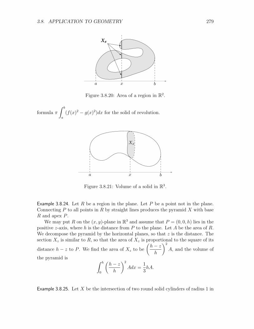
3.8. APPLICATION TO GEOMETRY 279
xa b
XxXxXx
Figure 3.8.20: Area of a region in R2.
formula π
∫ b
a
(f(x)2 − g(x)2)dx for the solid of revolution.
Xx
a bx
Figure 3.8.21: Volume of a solid in R3.
Example 3.8.24. Let R be a region in the plane. Let P be a point not in the plane.Connecting P to all points in R by straight lines produces the pyramid X with baseR and apex P .
We may put R on the (x, y)-plane in R3 and assume that P = (0, 0, h) lies in thepositive z-axis, where h is the distance from P to the plane. Let A be the area of R.We decompose the pyramid by the horizontal planes, so that z is the distance. Thesection Xz is similar to R, so that the area of Xz is proportional to the square of its
distance h− z to P . We find the area of Xz to be
(h− zh
)2
A, and the volume of
the pyramid is ∫ h
0
(h− zh
)2
Adx =1
3hA.
Example 3.8.25. Let X be the intersection of two round solid cylinders of radius 1 in

280 CHAPTER 3. INTEGRATION
0
h
z
P
R
Xz
area A
area
(h− zh
)2
A
Figure 3.8.22: Pyramid.
orthogonal position. We put the two cylinders in R3, by assuming the two cylindersto be x2 +y2 ≤ 1 and x2 +z2 ≤ 1. Then we decompose the solid by intersecting withthe planes perpendicular to the x-axis. The section Xx is a square of side length2√
1− x2 and therefore has area 4(1− x2). The volume of the intersection solid Xis ∫ 1
−1
4(1− x2)dx =16
3.
x √ 1−x2
1 −1−1 x
Figure 3.8.23: Orthogonal intersection of two cylinders.
Exercise 3.8.25. Explain the formula in Section 3.8.3 for the area of surface of revolutionby using suitable equidistant decomposition.
Exercise 3.8.26. Explain that if a solid is stretched by a factor A in the x-direction, by Bin the y-direction, and by C in the z-direction, then the volume of the solid is multipliedby the factor ABC.
Exercise 3.8.27. Find the volume of solid.

3.8. APPLICATION TO GEOMETRY 281
1. Ellipsoidx2
a2+y2
b2+z2
c2≤ 1.
2. Solid bounded byx2
a2+y2
b2− z2
c2= 1 and z = ±c.
3. Intersection of the sphere x2 + y2 + z2 ≤ 1 and the cylinder x2 + y2 ≤ x.
4. Solid bounded by x+ y + z2 = 1 and inside the first quadrant.
Exercise 3.8.28. Find the volume of solid.
1. A solid with a disk as the base, and the parallel sections perpendicular with thebase are equilateral triangles.
2. A solid with a disk as the base, and the parallel sections perpendicular with thebase are squares.
3. Cylinder cut by two planes, one is perpendicular to the cylinder and the other formangle α with the cylinder. The two planes do not intersect inside the cylinder.
4. Cylinder cut by two planes forming respective angles α and β with the cylinder.The two planes do not intersect inside the cylinder.
5. A wedge cut out of a cylinder, by two planes forming respective angles α and β withthe cylinder, such that the intersection of two planes is a diameter of the cylinder.
So far we used parallel lines and planes to construct the decomposition. We mayalso use equidistant curves and surfaces to construct the decomposition.
Example 3.8.26. We may decompose a region X in the plane by concentric circles.The decomposition is equidistant, with the radius r of the circles as the distance. Thesection Xr consists of the points in X of distance r from the origin and is typicallyan arc from angle φ(r) to angle ψ(r). The length of the arc Xr is (ψ(r)− φ(r))r, so
that the area of X is
∫ b
a
(ψ(r)− φ(r))rdr.
O
φ(r)
ψ(r)
a
rb
Xr
Figure 3.8.24: Equidistant decomposition by concentric circles.

282 CHAPTER 3. INTEGRATION
For example, for the disk centered at (1, 0) and of radius 1, we have φ =
− arccosr
2and ψ = arccos
r
2, r ∈ [0, 2]. The area of the disk of radius 1 is (taking
t = arccosr
2, r = 2 cos t)∫ 2
0
2r arccosr
2dr =
∫ 0
π2
2t(2 cos t)d(2 cos t) = 8
∫ π2
0
t cos t sin tdt
= 4
∫ π2
0
t sin 2tdt =
∫ π
0
u sinudu = π.
Example 3.8.27. Let X be a region in the right plane (i.e., the right side of y-axis).Let Y be the solid obtained by revolving X around the y-axis. We may use thecylinders centered at the y-axis to decompose Y . The decomposition is equidistant,with x as the distance. Let Xx be the intersection of X with the vertical linex × R. Then the section Yx is the cylinder obtained by revolving Xx around they-axis. The area of the section is 2πx(length of Xx). Therefore the volume of the
solid of revolution is 2π
∫ b
a
x(length of Xx)dx. In particular, if X is the region
between functions f(x) and g(x), where f(x) ≥ g(x) on [a, b], then the volume is
2π
∫ b
a
x(f(x)− g(x))dx.
x
y
X
Yx Xx
Figure 3.8.25: Equidistant decomposition by concentric cylinders.
For example, consider the solid torus in Example 3.8.17. The disk is the regionbetween x =
√a2 − (y − b)2 and x = −
√a2 − (y − b)2, for y ∈ [b− a, b + a]. If we
use the formula above (note that x and y are exchanged), we get the volume of thesolid torus
2π
∫ b+a
b−ay(2√a2 − (y − b)2)dy = 4π
∫ a
−a(t+ b)
√a2 − t2)dt
= 8π
∫ a
0
b√a2 − t2dt = 4π2a2b.

3.8. APPLICATION TO GEOMETRY 283
Exercise 3.8.29. Compute the volumes of the solids of revolution in Example 3.8.21 byusing the formula in Example 3.8.27.
Exercise 3.8.30. Compute the volumes of the solids of revolution in Exercise 3.8.23 byusing the formula in Example 3.8.27.
Exercise 3.8.31. Compute the volumes of the solids of revolution in Exercise 3.8.24 byusing the formula in Example 3.8.27.
Exercise 3.8.32. After Example 3.8.21, we presented the formula for computing the volumeof a solid obtained by revolving a region in R2 bounded by a parameterized curve. Canyou derive the similar formula by using the idea from Example 3.8.27?
Exercise 3.8.33. In Section 3.8.4 and Example 3.8.27, we have two ways of computing thevolume of a solid of revolution. For the following simple case, explain that the two waysgive the same result: Let f(x) be and invertible non-negative function on [0, a], such thatf(a) = 0 and both f(x) and f−1(y) are continuously differentiable. The solid is obtainedby revolving the region between the graph of f and the two axis.
Example 3.8.28. Finally, we compute the size of high dimensional objects. Let αnbe the volume of the n-dimensional sphere Sn of radius 1. Then
α0 = 2, α1 = 2π, α2 = 4π.
Moreover, the n-dimensional sphere of radius r has volume αnrn.
To compute αn, we decompose Sn by intersecting with “horizontal hyperplanes”.The hyperplanes are indexed by the angle t. The section at angle t is the (n − 1)-dimensional sphere Sn−1 of radius cos t, and form an equidistant decomposition. Infact, the angle t can be used to measure the distance between the sections. Since
the section at t has volume αn−1 cosn−1 t and the range of t is[−π
2,π
2
], we conclude
that
αn =
∫ π2
−π2
αn−1 cosn−1 tdt = 2αn−1In−1,
where In−1 =
∫ π2
0
cosn−1 tdt =
∫ π2
0
sinn−1 tdt has been computed in Example 3.5.14
I2k =(2k)!
22k+1(k!)2π, I2k+1 =
22k(k!)2
(2k + 1)!.
Thus
αn = 2αn−1In−1 = 4αn−2In−1In−2 = 4αn−2π
2(n− 1)=
2π
n− 1αn−2.

284 CHAPTER 3. INTEGRATION
By the values of α1 and α2, we conclude that
αn =
(2π)
n2
2 · 4 · · · (n− 2), if n is even,
2(2π)n−1
2
1 · 3 · · · (n− 2), if n is odd.
1
cos t
Sn−1 of radius cos t
t
Figure 3.8.26: Decomposing n-dimensional sphere of radius 1.
Exercise 3.8.34. Let βn be the volume of the ball Bn of radius 1.
1. Similar to Example 3.8.28, use the intersection with horizontal hyperplanes to derivethe relation between βn and βn−1. Then use the special values β1 and β2, andExample 3.5.14 to compute βn.
2. Use the decomposition of Bn by concentric (n − 1)-dimensional spheres to derivethe relation between βn and αn−1. Then use Example 3.8.28 to find βn.
The two methods should give the same result.
Exercise 3.8.35. Suppose R is a region in Rn−1 with volume. Suppose P is a point in Rnof distance h from Rn−1. By connecting P to all points of R by straight lines, we get apyramid X with base R and apex P . Find the relation between the volumes of X and R.
3.9 Polar Coordinate
The polar coordinate locates a point on the plane by its distance r to the originand the angle θ indicating the direction from the viewpoint of origin. It is roughlyrelated to the cartesian coordinates (x, y) by
x = r cos θ, y = r sin θ; r =√x2 + y2, θ = arctan
y
x.
We say “roughly” because the relation between (x, y) and (r, θ) is not a one-to-onecorrespondence. For example, the last formula literally restricts θ, as the value of

3.9. POLAR COORDINATE 285
inverse tangent function, to be within(−π
2,π
2
). In fact, the angle for a point in the
plane is unique only up to adding an integer multiple of 2π, and is more preciselydetermined by
(cos θ, sin θ) =(x, y)√x2 + y2
.
Another way to say this is that θ is unique if we restrict to [0, 2π) (or [−π, π), etc.).For the convenience of presenting polar equations, we also allow r to be negative,
by specifying that (−r, θ) and (r, θ + π) represent the same point. In other words,(−r, θ) and (r, θ) are symmetric with respect to the origin. The cost of such extensionis more ambiguity in the polar coordinates of a point because all the followingrepresent the same point
(r, θ), (−r, θ ± π), (r, θ ± 2π), (−r, θ ± 3π), . . . .
3.9.1 Curves in Polar Coordinate
Example 3.9.1. The equation r = c is the circle of radius |c| centered at the origin.The equation θ = c is a straight line passing through the origin.
θ = cr = c
dr
αθ
Figure 3.9.1: r = c, θ = c, and polar equation for general straight line.
The equation for a general straight line is
r =d
cos(α− θ).
Moreover, r = a cos θ is the circle of diameter a passing through the origin.
O
r = cos θ
aθ r
θ
0 π2
3π2 2π
Figure 3.9.2: Circle r = a cos θ.
Exercise 3.9.1. Find the cartesian equation.

286 CHAPTER 3. INTEGRATION
1. r = 2.
2. r = −2.
3. r = sin θ.
4. r sin θ = 1.
5. r = tan θ sec θ.
6. r = cos θ + sin θ.
Exercise 3.9.2. Find the polar equation.
1. x = 1.
2. y = −1.
3. x+ y = 1.
4. x = y2.
5. x2 + y2 = x.
6. xy = 1.
Exercise 3.9.3. What is the polar equation of the curve obtained by flipping r = f(θ) withrespect to the origin? Then use your conclusion to find the curve r = − cos θ.
Exercise 3.9.4. What is the relation between the curves r = f(θ) and r = −f(θ + π)?
Exercise 3.9.5. What is the polar equation of the curve obtained by rotating r = f(θ) byangle α? Then use your conclusion to answer the following.
1. What is the curve r = sin θ?
2. Find the polar equation for a general circle passing through the origin.
Exercise 3.9.6. Find the polar equation of a general circle.
Example 3.9.2. The Archimedean spiral is r = θ. Note that r < 0 when θ < 0, sothat a flipping with respect to the origin is needed when we draw the part of thespiral corresponding to θ < 0. The symmetry with respect to the y-axis is due tothe fact that if (r, θ) satisfies r = θ, then (−r,−θ) also satisfies r = θ.
The Fermat’s spiral is r2 = θ. The symmetry with respect to the origin is dueto the fact that if (r, θ) satisfies r2 = θ, then (−r, θ) also satisfies r2 = θ.
(r, θ)
(r,−θ)
(−r,−θ)
(−r, θ)
Figure 3.9.3: Spirals r = θ and r2 = θ.
Example 3.9.3. The curve r = 1 + cos θ is a cardioid. Its clockwise rotation by 90◦ isanother cardioid r = 1 + sin θ. More generally, the curve r = a+ cos θ is a limacon.

3.9. POLAR COORDINATE 287
The curve intersects itself when |a| < 1 and does not intersect itself when |a| > 1.The symmetry with respect to the x-axis is due to the fact that if (r, θ) satisfiesr = a+ cos θ, then (r,−θ) also satisfies the equation.
θ = 0
π2
3π2
π
r = 1 + cos θ r = 1 + sin θ
0.4
1
1.5
Figure 3.9.4: Cardioids and limacons r = a+ cos θ, a = 0.4, 1, 1.5.
The cardioid originates from the following geometrical construction. Consider acircle C of diameter 1 rolling outside of a circle A of equal diameter 1. This is thesame as the circle rolling inside a big circle B of diameter 3. The track traced by apoint on C is the cardioid. Note that the origin O of the polar coordinate shouldbe a point on A, not the center of A.
θθθ
θ
θ
O 1 2
A C
Bco
s θ
1
Figure 3.9.5: Origin of the cardioid.
If we imagine the rolling circle C as part of a rolling disk D, and we fix a pointin D of distance d from the center of C. Then the track tranced by the point is thelimacon r = 1 + 2d cos θ, with the origin of the polar coordinate being a point ofdistance d form the center of A.
Example 3.9.4. The curve r = cos 2θ is the four-leaved rose, and r = cos 3θ is thethree-leaved rose. The circle r = cos θ can be considered as the one-leaved rose.

288 CHAPTER 3. INTEGRATION
In general, the curve r = cosnθ can be described as follows. For θ in the arc
I =[− π
2n,π
2n
], the value of r goes from 0 to 1 and then back to 0, so that the
corresponding curve is one leaf occupyingπ
nangle of the whole circle. This is the
leaf in[−π
4,π
4
]for n = 2 and in
[−π
6,π
6
]for n = 3. For θ in the second arc I +
π
n,
we need to rotate this first leaf by angleπ
nand then flipping with respect to the
origin (because r becomes negative), which gives a leaf occupying I +π
n+ π. This
is the leaf in
[5π
4,7π
4
]for n = 2 and in
[7π
6,9π
6
]for n = 3. For θ in the third arc
I +2π
n, we get the leaf obtained by rotating the first leaf by angle
2π
n(no flipping
needed now because r becomes non-negative again), which gives a leaf occupying
I +2π
n. This is the leaf in
[3π
4,5π
4
]for n = 2 and in
[3π
6,5π
6
]for n = 3. Keep
going, we see two distinct patterns depending on the parity of n.
1
2
3
4
θ = 0θ = π
θ = 3π2
θ = π2
1
2
3
θ = 0
θ = π3
θ = 2π3
Figure 3.9.6: Four-leaved rose r = cos 2θ and three-leaved rose r = cos 3θ.
More generally, we may consider r = cos pθ. Again we get first leaf occupying
I =
[− π
2p,π
2p
], the second leaf occupying I+
π
p+π, the third leaf occupying I+
2π
p,
etc. The pattern could be very complicated, depending on whether p is rational orirrational, and in case p is rational, the parity of the numerator and denominator ofp.
Finally, r = sin pθ is obtained by rotating r = cos 2θ byπ
2p. We also get many
leaved roses by other rotations.
Exercise 3.9.7. Describe the curve.

3.9. POLAR COORDINATE 289
Figure 3.9.7: Many leaved roses r = sin 2θ and r = sin 32θ.
1. r = −θ.
2. r = θ + π.
3. r = 2θ.
4. r2 = −θ.
5. r2 = 4θ.
6. r2 = θ + π.
7. er = θ.
8. rθ = 1.
9. r = 2 + cos θ.
10. r = 2 + 3 cos θ.
11. r = 2− cos θ.
12. r = cos θ + sin θ.
13. r = 1 + cos θ + sin θ.
14. r = cos 4θ.
15. r = 2 sin 5θ.
16. r = −3 sin 6θ.
17. r = sin 2θ − cos 2θ.
18. r = sin 2θ + 2 cos 2θ.
19. r = cos4
3θ.
20. r = sin5
3θ.
21. r = cos1
3θ.
22. r = cos2
3θ.
23. r = cos2
3θ + sin
2
3θ.
24. r2 = sin 2θ.
25. r2 = − cos 4θ.
26. r = 1 + 2 cos1
2θ.
27. r = 2 + cos1
2θ.
3.9.2 Geometry in Polar Coordinate
The curve r = f(θ) for θ ∈ [α, β] is the parameterized curve
x = f(θ) cos θ, y = f(θ) sin θ, θ ∈ [α, β]
in the cartesian coordinate. The length of the curve is∫ β
α
√(f(θ) cos θ)′2 + (f(θ) sin θ)′2dθ =
∫ β
α
√f 2 + f ′2dθ.
For the area in terms of polar coordinate, assume f ≥ 0 and consider the regionX[α,β](f) bounded by r = f(θ), θ ∈ [α, β], and the rays θ = α and θ = β. Using theidea of Section 3.1.1, let A(θ) be the area of the region X[α,θ](f). Then the changeA(θ + h) − A(θ) is the area of X[θ,θ+h](f). Since X[θ,θ+h](f) is sandwiched betweenfans of angle between θ, θ + h and radii m = min[θ,θ+h] f , M = max[θ,θ+h] f , we get
1
2m2h ≤ A(θ + h)− A(θ) ≤ 1
2M2h.

290 CHAPTER 3. INTEGRATION
Here the left and right sides are the known areas of the fans. The inequality is thesame as
1
2m2 ≤ A(θ + h)− A(θ)
h≤ 1
2M2.
O
α
β
θ
θ + h
Mm
Figure 3.9.8: Estimate the change of area.
If f is continuous, then limh→0m = limh→0M = f(θ). By the sandwich rule, weget
A′(θ) =1
2f(θ)2.
Therefore the area of X[α,β](f) is
A(β) =1
2
∫ β
α
f(θ)2dθ.
Example 3.9.5. The cardioid r = 1 + sin θ has length∫ 2π
0
√(1 + sin θ)2 + (1 + sin θ)′2dθ =
∫ 2π
0
√2(1 + sin θ)dθ
=
∫ − 34π
14π
√2(1 + cos 2t)d
(π2− 2t
)= 4
∫ 14π
− 34π
| cos t|dt = 4
∫ π
0
cos tdt = 8.
The region enclosed by the cardioid has area
1
2
∫ 2π
0
(1 + sin θ)2dθ =1
2
∫ 2π
0
(1 + 2 sin θ + sin2 θ)dθ =3
2π.
Example 3.9.6. Let p >1
2. Then one leaf of the rose r = cos pθ is from the angle

3.9. POLAR COORDINATE 291
− π
2pto the angle
π
2p. The length of the leaf is
∫ π2p
− π2p
√(cos pθ)2 + (cos pθ)′2dθ =
∫ π2p
− π2p
√cos2 pθ + p2 sin2 pθdθ
=
∫ π2
−π2
√p−2 cos2 t+ sin2 tdt
=1
2
∫ 2π
0
√1 + (p−2 − 1) cos2 tdt.
This is the elliptic integral in Example 3.8.1. Moreover, the area of the leaf is
1
2
∫ π2p
− π2p
(cos pθ)2dθ =π
4p.
Example 3.9.7. The cardioid r = 1 + cos θ and the circle r = 3 cos θ intersect at
θ = ±π3
. The area of the region outside the cardioid and inside the circle is
1
2
∫ π3
−π3
((3 cos θ)2 − (1 + cos θ)2)dθ = π.
π3
−π3
Figure 3.9.9: Ourside cardioid r = 1 + cos θ and inside circle r = 3 cos θ.
Example 3.9.8. We try to find the volume of the solid of revolution obtained byrevolving the region between the two leaves of the limacon r = a+ cos θ, 0 < a < 1,around the x-axis. In the cartesian coordinate, the curve is parameterized by
x = (a+ cos θ) cos θ, y = (a+ cos θ) sin θ, θ ∈ [0, π].
Let θ = α at the origin O. Then the volume we are looking for is the volume ofthe solid of revolution from θ = 0 to θ = α, subtracting the volume of the solid of

292 CHAPTER 3. INTEGRATION
revolution from θ = α to θ = π. As θ goes from 0 to α, we are moving opposite to
the direction of the x-axis. Therefore the first volume is −π∫ θ=α
θ=0
y2dx. As θ goes
from α to π, we are moving in the direction of the x-axis. Therefore the second
volume is π
∫ θ=π
θ=α
y2dx. We conclude that the volume we are looking for is
−π∫ θ=α
θ=0
y2dx− π∫ θ=π
θ=α
y2dx = −π∫ θ=π
θ=0
y2dx
= −π∫ π
0
(a+ cos θ)2 sin2 θd[(a+ cos θ) cos θ]
= −π∫ π
0
(a+ cos θ)2(1− cos2 θ)(a+ 2 cos θ)d(cos θ)
= −π∫ −1
1
(a+ t)2(1− t2)(a+ 2t)dt =4
3πa(a2 + 1).
Oθ = 0θ = π
θ = α
Figure 3.9.10: Revolving the region between two leaves of a limacon.
Exercise 3.9.8. What is the length of lemicon? What is the area of the region enclosed bylemicon? Note that for |c| > 1, we have two parts of the lemicon and two regions.
Exercise 3.9.9. Find length of the part of the cardioid r = 1 + cos θ in the first quadrant.Moreover, find the area of the region enclosed by this part and the two axes.
Exercise 3.9.10. Find the area of the region enclosed by strophoid r = 2 cos θ − sec θ.
Exercise 3.9.11. Find length.
1. r = θ, θ ∈ [0, π]. 2. r = θ2, θ ∈ [0, π]. 3. r = eθ, θ ∈ [0, 2π].
Exercise 3.9.12. Find area.
1. Bounded by r = θ, θ ∈ [0, π] and the x-axis.

3.10. APPLICATION TO PHYSICS 293
2. Outside r = 1 and inside r = 2 cos θ.
3. Inside r = 1 and outside r = 2 cos θ.
4. Inside both r = 1 and r = 1 + cos θ.
5. Outside r = 3 sin θ and inside r = 2− sin θ.
6. Inside both r = cos 2θ and r = sin 2θ.
7. Inside both r = 1 + c cos θ and r = 1 + c sin θ, |c| < 1.
8. Inside both r = 1 + c cos θ and r = 1− c cos θ, |c| < 1.
9. Inside both r2 = cos 2θ and r2 = sin 2θ.
10. Outside r = 1 and inside r = 2 cos 3θ.
11. Between the two loops of r = 1 + 2 cos 3θ.
3.10 Application to Physics
3.10.1 Work and Pressure
Integration is also widely used to compute physical quantities. If under a constantforce F , an object moves by a distance d in the direction of the force, then the workdone by the force is Fd. In general, however, the force may vary. For simplicity,assume the object moves along the x-axis, from x = a to x = b, and a horizontalforce F (x) is applied when the object is at location x. Then the work done bythe force when the objects moves a little bit from x to x + ∆x is approximately∆W ≈ F (x)∆x.
Similar to the earlier argument, let W (x) be the work done by the force whenthe object moves from a to x. Since the work is additive, we have ∆W = W (x +
∆x)−W (x). The approximation∆W
∆x≈ F (x) becomes more accurate as ∆x→ 0,
and we get an equality after taking the limit
W ′(x) = lim∆x→0
W (x+ ∆x)−W (x)
∆x= lim
∆x→0
∆W
∆x= F (x).
This implies that the work done for the whole trip from a to b is
W (b) =
∫ b
a
F (x)dx.
Example 3.10.1. Suppose one end of spring is fixed and the other end is attachedto an object. In the natural position, when the spring is neither stretched norcompressed, no force is exercised on the object. When the position of the object

294 CHAPTER 3. INTEGRATION
deviate from the natural position by x, however, Hooke’s law says that the springexercises a force F (x) = −kx on the object. Here k is the spring constant, and thenegative sign indicates that the direction of the force is opposite to the direction ofthe deviation.
If the object starts at distance a from its natural position, then the work doneby the spring in pulling the object to its natural position is∫ a
0
kxdx =k
2a2.
Here we use the positive sign because the direction of movement is the same as thedirection of the force.
The argument about the work done by a force is quite typical. In general, if aquantity is additive, then the quantity can be decomposed into small pieces. Theestimation of each small piece tells us the change of the quantity. The whole quantityis then the integration of the change.
In the subsequent examples, we will only analyze a small piece of an additivequantity. We will omit the limit part of the argument and directly write down thecorresponding integration.
Example 3.10.2. We want to find the work it takes to pump a bucket of liquid outof the top of the bucket.
∆x
r
R
h
H
x
Figure 3.10.1: Bucket of liquid.
Suppose the bucket has base diameter r, top diameter R, and height H. Supposethe liquid has density ρ and depth h. We decompose liquid into horizontal sections.At distance x from the top, the section is a disk of radius r(x) satisfying
r(x)− rR− r
=H − xH
.
The liquid of thickness ∆x and at distance x from the top has (approximate) weightgρπr(x)2∆x (g is the gravitational constant). The work it takes to lift this piece

3.10. APPLICATION TO PHYSICS 295
of liquid to the top of bucket is ∆W ≈ (gρπr(x)2∆x)x = πgρxr(x)2∆x. Since theliquid spans from x = H − h to x = H, the total work needed is
W = πgρ
∫ H
H−hxr(x)2dx =
πgρ
H2
∫ H
H−hx [(R− r)(H − x) + rH]2dx
= πgρH2R2
(a2b+
1
2a(2a− 3b)b2 +
1
3(1− a)(1− 3a)b3 − 1
4(1− a)2b4
),
where a =r
Rand b =
h
H.
Example 3.10.3. We want to find the force exercised by water on a dam.Let ρ be the density of water. At the depth x, the pressure of water is ρx per unit
area. Now suppose the dam is a vertical trapezoid with base length l, top length L,and height H. We decompose dam into horizontal sections. At distance x from thetop, the section is a strip of height ∆x and length l(x) satisfying
l(x)− lL− l
=H − xH
.
The force exercised on the strip is ∆F ≈ (ρx)l(x)∆x. Since the water spans fromx = 0 to x = H, the total force
F = ρ
∫ H
0
xl(x)dx = ρ
∫ H
0
x
(L− L− l
Hx
)dx =
1
6ρH2(L+ 2l).
l
L
l(x)∆xH
x
Figure 3.10.2: Hydraulic dam.
Exercise 3.10.1. A spring has natural length a. If the force F is needed to stretch thespring to length b, how muck work is needed to stretch the spring from the natural lengthto the length b?
Exercise 3.10.2. A ball of radius R is full of liquid of density ρ. Due to the gravity, theliquid leaks out of a hole at the bottom of the ball. How much work is done by the gravityin draining all the liquid?

296 CHAPTER 3. INTEGRATION
Exercise 3.10.3. A circular disk of radius r is fully submerged in liquid of density ρ, suchthat the center of the disk is at depth h. What is the force exercised by the liquid on oneside of the plate? Note that the plate may be inclined at some angle.
Exercise 3.10.4. A ball of radius r is fully submerged in liquid of density ρ, such that thecenter of the disk is at depth h. What is the force exercised by the liquid on the ball?
Exercise 3.10.5. A cable of mass m and length l has a mass M tied to the lower end. Howmuch word is done in using the cable to lift the mass M to the top end of the cable?
Exercise 3.10.6. Newton’s law of gravitation says that two bodies with masses m and M
attract each other with a force F =gmM
d2, where d is the distance between the bodies.
Suppose the radius of the earth is R and the mass is M . How much work is needed tolaunch a satellite of mass m vertically to a circular orbit of height H? What is the minimalinitial velocity needed for the satellite to escape the earth’s gravity?
3.10.2 Center of Mass
Consider n masses m1,m2, . . . ,mn distributed at the locations x1, x2, . . . , xn alonga straight line. The center of mass is
x =m1x2 +m2x2 + · · ·+mnxn
m1 +m2 + · · ·+mn
.
The center has the physical meaning that the total moment of the system withrespect to x is zero, or the system is balanced with respect to x.
Now suppose we have masses distributed throughout an interval [a, b], with thedensity ρ(x) at location x. We partition the interval into small pieces
P : a = x0 < x1 < x2 < · · · < xn = b.
Then the system is decomposed into n pieces. The i-th piece can be approximatelyconsidered as a mass mi = ρ(x∗i )(xi − xi−1) located at x∗i , for some x∗i ∈ [xi−1, xi].The whole system is approximated by the system of n pieces, and has approximatecenter of mass
xP =
∑ni=1 ρ(x∗i )(xi − xi−1)x∗i∑ni=1 ρ(x∗i )(xi − xi−1)
.
The denominator is the Riemann sum of the function xρ(x) and the numerator is theRiemann sum of the function ρ(x) (see the beginning of Section 3.3.1). Thereforeas the partition gets more and more refined, the limit becomes the center of mass
x =
∫ b
a
xρ(x)dx∫ b
a
ρ(x)dx
.

3.10. APPLICATION TO PHYSICS 297
The center of mass can be extended to higher dimensions, simply by consideringeach coordinate separately. For example, the system of n masses m1,m2, . . . ,mn at(x1, y1), (x2, y2), . . . , (xn, yn) in the plane has the center of mass (x, y) given by
x =
∑mixi∑mi
, y =
∑miyi∑mi
.
Now consider masses distributed along a curve (x(t), y(t)), t ∈ [a, b], with the densityρ(t) at location t. Take a partition P of [a, b]. The curve is approximated bystraight line segments connecting (x(ti−1), y(ti−1)) to (x(ti), y(ti)). The i-th straightline segment has length ∆si =
√(x(ti)− x(ti−1))2 + (y(ti)− y(ti−1))2 and can be
approximately considered as a mass mi = ρ(t∗i )∆si located at (x(t∗i ), y(t∗i )), for somet∗i ∈ [ti−1, ti]. The whole system is approximated by the system of n pieces, and hasapproximate center of mass
xP =
∑ni=1(ρ(t∗i )∆si)x(t∗i )∑n
i=1 ρ(t∗i )∆si, yP =
∑ni=1(ρ(t∗i )∆si)y(t∗i )∑n
i=1 ρ(t∗i )∆si.
As the partition gets more and more refined, the limit becomes the center of mass
x =
∫ b
a
x(t)ρ(t)ds∫ b
a
ρ(t)ds
, y =
∫ b
a
y(t)ρ(t)ds∫ b
a
ρ(t)ds
, ds =√x′(t)2 + y′(t)2dt.
Example 3.10.4. For constant density ρ(x) = ρ distributed on the interval, the centerof mass is the middle point
x =
∫ b
a
xρdx∫ b
a
ρdx
=ρ
1
2(b2 − a2)
ρ(b− a)=a+ b
2.
If the density is ρ(x) = λ+ µx, which is linearly increasing, then the center of massis
x =
∫ b
a
x(λ+ µx)dx∫ b
a
(λ+ µx)dx
=3λ(a+ b) + 2µ(a2 + ab+ b2)
3(2λ+ µ(a+ b)).
Example 3.10.5. Consider the semi-circular curve of radius r and constant density ρ.We have
x = r cos θ, y = r sin θ, ds = rdθ, 0 ≤ θ ≤ π,
298 CHAPTER 3. INTEGRATION
and the center of mass is
x =
∫ π
0
(r cos θ)ρrdθ∫ π
0
ρrdθ
= 0, y =
∫ π
0
(r sin θ)ρrdθ∫ π
0
ρrdθ
=2r
π.
Exercise 3.10.7. Find the center of mass of the parabola y = x2, x ∈ [0, 2], of constantdensity.
Exercise 3.10.8. Find the center of mass of a triangle of constant density and with verticesat (−1, 0), (0,
√15) and (7, 0).
Exercise 3.10.9. Let m[a,b] and x[a,b] be the mass and the center of mass of a distributionof masses on [a, b] with the density ρ(x). Let [a, b] = [a, c] ∪ [c, b] and similarly introducem[a,c], m[c,b], x[a,c], x[c,b]. Show that the center of mass has the distribution property
m[a,b] = m[a,c] +m[c,b], x[a,b] =m[a,c]x[a,c] +m[c,b]x[c,b]
m[a,c] +m[c,b].
Does the property extend to curves in R2?

Chapter 4
Series
4.1 Series of Numbers
A series is an infinite sum
∞∑n=1
an = a1 + a2 + a3 + · · · .
The following are some examples.
∞∑n=0
rn = 1 + r + r2 + r3 + · · ·+ rn + · · · ,
∞∑n=1
n = 1 + 2 + 3 + · · ·+ n+ · · · ,
∞∑n=1
1
n(n+ 1)=
1
1 · 2+
1
2 · 3+
1
3 · 4+ · · ·+ 1
n(n+ 1)+ · · · ,
∞∑n=1
1
np= 1 +
1
2p+
1
3p+ · · ·+ 1
np+ · · · ,
∞∑n=1
(−1)n+1
n= 1− 1
2+
1
3− · · ·+ (−1)n+1
n+ · · · ,
∞∑n=0
1
n!= 1 +
1
1!+
1
2!+ · · ·+ 1
n!+ · · · .
Like sequences, series do not have to start at n = 1. For example, it is moreconvenient for the geometric series
∑∞n=0 r
n to start at n = 0.
299

300 CHAPTER 4. SERIES
4.1.1 Sum of Series
Definition 4.1.1. The partial sum of a series∑∞
n=1 an is
sn =n∑i=1
ai = a1 + a2 + · · ·+ an.
If the partial sum converges, then the series converges and has sum (or value)
∞∑n=1
an = limn→∞
sn.
If the partial sum diverges, then the series diverges.
If finitely many terms in a series are modified, added or dropped, then the newpartial sum s′n and the original partial sum sn are related by s′n = sn+n0 + C forsome constants n0 and C. This implies that the convergence of series is not affected,although the sum may be affected.
The arithmetic properties of the sequence limit implies∑(an + bn) =
∑an +
∑bn,
∑can = c
∑an.
However, there is no formula for∑anbn or
∑ anbn
.
Example 4.1.1. Let sn = 1 + r + r2 + · · ·+ rn be the partial sum of geometric series∑∞n=0 r
n. Then
(1− r)sn = (1 + r + r2 + · · ·+ rn)− (r + r2 + r3 + · · ·+ rn+1) = 1− rn+1.
Therefore sn =1− rn+1
1− rand
∞∑n=0
rn =
1
1− r, if |r| < 1,
diverges, if |r| ≥ 1.
Example 4.1.2. The computation in Example 1.3.1 gives the partial sum of∑ 1
n(n+ 1).
1
1 · 2+
1
2 · 3+· · ·+ 1
n(n+ 1)=
(1− 1
2
)+
(1
2− 1
3
)+· · ·+
(1
n− 1
n+ 1
)= 1− 1
n+ 1.
Therefore∞∑n=1
1
n(n+ 1)= lim
n→∞
(1− 1
n+ 1
)= 1.

4.1. SERIES OF NUMBERS 301
Example 4.1.3. Example 2.7.5 shows that the partial sum of∑ 1
n!satisfies |sn−e| =
|Rn(1)| ≤ e
(n+ 1)!, which implies
∑∞n=0
1
n!= e. Exercise 1.3.18 gives an alternative
argument. Of course the argument, which uses the Lagrange form of the remainder
(Theorem 2.7.1), can be extended to the series∑ xn
n!. The partial sum satisfies
|sn − ex| = |Rn(x)| = ec
(n+ 1)!|x|n+1 ≤ e|x|
(n+ 1)!|x|n+1, |c| < |x|.
Since for fixed x, the right side converges to 0 as n → ∞, we conclude that∑∞n=0
xn
n!= ex.
Exercise 4.1.1. Suppose the partial sum sn =n
2n+ 1. Find the series
∑an and its sum.
Exercise 4.1.2. Decimal expressions for rational numbers have repeating patterns. Forexample, we have
1.234 = 1.2343434 · · · = 1.2 +34
1000+
34
100000+
34
10000000+ · · ·
= 1.2 +34
1000
∞∑n=0
1
100n= 1.2 +
34
1000
1
1− 1
100
=611
495.
1. Find rational expressions for 1.23, 1.230, 1.023.
2. Final the decimal based series representing the rational numbers5
12,
43
35.
Exercise 4.1.3. What is the total area of infinitely many disks?
θ
a
Exercise 4.1.4. The Sierpinski carpet is obtained from the unit square by successivelydeleting “one third squares”. Find the area of the carpet.

302 CHAPTER 4. SERIES
Exercise 4.1.5. Two lines L and L′ form an angle θ at P . A boy starts on L at distance afrom P and walk to L′ along shortest path. After reaching L′, he walks back to L alongshortest path. Then he walks to L′ again along shortest path, and keeps walking back andforth. What is the total length of his trip?
Exercise 4.1.6. Find the area between curves y = xn and y = xn+1 and use this to conclude
that∑∞
n=1
1
n(n+ 1)= 1.
Exercise 4.1.7. Compute the partial sum and the sum of series.
1.∑∞
n=1 nrn.
2.∑ 2n + (−1)n3n−1
5n+1.
3.∑∞
n=0
1
(a+ nd)(a+ (n+ 1)d).
4.∑∞
n=2
1
n(n+ 1)(n+ 2).
5.∑∞
n=2 log
(1− 1
n2
).
6.∑∞
n=1
n
(n+ 1)!.
Exercise 4.1.8. Suppose xn > 0. Compute∑∞
n=1
xn(1 + x1)(1 + x2) · · · (1 + xn)
.
Exercise 4.1.9. The Fibonacci sequence 1, 1, 2, 3, 5, . . . is defined recursively by a0 = a1 = 1,an = an−1 + an−2. Prove the following
1
an−1an+1=
1
an−1an− 1
anan+1,
∞∑n=2
1
an−1an+1= 1,
∞∑n=2
anan−1an+1
= 2.
Exercise 4.1.10. Use the Lagrange form of the remainder to show that the Taylor series
for1
1− xconverges for |x| < 1.
Exercise 4.1.11. Use the Lagrange form of the remainder to show that the Taylor seriesfor cosx and sinx converge for any x
∞∑n=0
(−1)nx2n
(2n)!= cosx,
∞∑n=0
(−1)nx2n+1
(2n+ 1)!= sinx.
4.1.2 Convergence of Series
Theorem 4.1.2. If∑an converges, then limn→∞ an = 0.
This is a consequence of
limn→∞
an = limn→∞
(sn − sn−1) = limn→∞
sn − limn→∞
sn−1 = s− s = 0.

4.1. SERIES OF NUMBERS 303
By the theorem, the series∑
1,∑n,∑
(−1)n,∑ n
n+ 1diverge. By Example
1.1.20, the series∑
sinna converges if and only if a is an integer multiple of π.If an ≥ 0 for sufficiently large n, then the partial sum sequence is increasing for
large n, and Theorem 1.3.2 becomes the following.
Theorem 4.1.3. If an ≥ 0, then∑an converges if and only if the partial sums are
bounded.
Example 4.1.4. The terms in the series∑
=1
npare positive. Therefore the con-
vergence is equivalent to the boundedness of the partial sum. For p ≥ 2, we have1
np<
1
(n− 1)nand the following bound from Examples 1.3.1 and 4.1.2
1
1p+
1
2p+ · · ·+ 1
np≤ 1 +
1
1 · 2+
1
2 · 3+ · · ·+ 1
(n− 1)n= 2− 1
n< 2.
By Theorem 4.1.3, therefore, the series converges for p ≥ 2.For p = 1, we used Cauchy criterion in Example 1.3.8 to show that the harmonic
series∑ 1
ndiverges.
Example 4.1.5. The even partial sum of the series∑ (−1)n+1
nis the partial sum of
the series ∑(1
2n− 1− 1
2n
)=
(1− 1
2
)+
(1
3− 1
4
)+ · · · .
The terms of the series above are positive, and the partial sum has upper bound
1− 1
2+
1
3−· · ·+ 1
2n− 1− 1
2n= 1−
(1
2− 1
3
)−· · ·−
(1
2n− 2− 1
2n− 1
)− 1
2n< 1.
By Theorem 4.1.3,∑(
1
2n− 1− 1
2n
)converges. This means that the even partial
sum s2n of∑ (−1)n+1
nconverges. By s2n+1 = s2n +
1
2n+ 1, the odd partial sum
s2n+1 converges to the same limit. Therefore∑ (−1)n+1
nconverges.
Exercise 4.1.12. Show the divergence of∑ 1
n√a
and∑ n
2n− 1.
Exercise 4.1.13. Determine convergence.

304 CHAPTER 4. SERIES
1. 1 +1
2− 1
3+
1
4+
1
5− 1
6+ · · · .
2. 1 +1
2− 2
3+
1
4+
1
5− 2
6+ · · · .
3. 1 +1
22+
1
33+
1
44+ · · · .
4. 1 +1√1 · 2
+1√3 · 4
+1√5 · 6
+ · · · .
Exercise 4.1.14. Use Theorem 4.1.3 to argue about the convergence of∑rn for 0 ≤ r < 1
and∑ 1
n!.
Exercise 4.1.15. What is wrong with the following calculation?
0 = 0 + 0 + 0 + · · ·= (1− 1) + (1− 1) + (1− 1) + · · ·= 1− 1 + 1− 1 + 1− 1 + · · ·= 1 + (−1 + 1) + (−1 + 1) + (−1 + 1) + · · ·= 1 + 0 + 0 + 0 + · · · = 1.
We used the Cauchy criterion (Theorem 1.3.3) for the divergence of harmonic
series∑ 1
n. In general, applying the Cauchy criterion to the partial sum shows that∑
an converges if and only if for any ε ≥ 0, there is N , such that (since |sm − sn| issymmetric in m and n, we may always assume n > m)
n > m > N =⇒ |sm − sn| = |am+1 + am+2 + · · ·+ an| < ε.
We may further modify the criterion by taking m+ 1 to be m.
Theorem 4.1.4 (Cauchy Criterion). A series∑an converges if and only if for any
ε > 0, there is N , such that
n ≥ m > N =⇒ |am + am+1 + · · ·+ an| < ε.
Theorem 4.1.2 is a special case of the Cauchy criterion by taking m = n.
4.2 Comparison Test
Series∑an are very much like improper integrals
∫ +∞
a
f(x)dx. The two can be
compared in two aspects. First the convergence of the two can be compared, through
the integral test. Second all the convergence theorems for
∫ +∞
a
f(x)dx, such as the
comparison test, Dirichlet test and Abel test, have parallels for the convergence ofseries.

4.2. COMPARISON TEST 305
4.2.1 Integral Test
Theorem 4.2.1 (Integral Test). Suppose f(x) is a decreasing function on [1,+∞)satisfying limx→+∞ f(x) = 0. Then
f(1) + f(2) + · · ·+ f(n) =
∫ n
1
f(x)dx+ γ + εn,
for a constant 0 ≤ γ ≤ f(1) and a decreasing sequence εn converging to 0. In partic-
ular, the series∑f(n) converges if and only if the improper integral
∫ +∞
a
f(x)dx
converges.
Let
xn = f(1) + f(2) + · · ·+ f(n)−∫ n
1
f(x)dx.
By f decreasing, we get
xn − xn−1 = f(n)−∫ n
n−1
f(x)dx ≤ 0,
xn − f(n) = f(1) + · · ·+ f(n− 1)−∫ n
1
f(x)dx ≥ 0
=n−1∑k=1
(f(k)−
∫ k+1
k
f(x)dx
)≥ 0.
The first inequality implies xn is decreasing, and the second inequality implies xn ≥f(n) ≥ 0. Therefore limxn = γ converges, and the theorem follows. We have0 ≤ γ ≤ x1 = f(1).
Example 4.2.1. For p > 0, the function1
xpis decreasing and converges to 0 as
x→ +∞. By Theorem 4.2.1, therefore, the series∑ 1
npconverges if and only if the
improper integral
∫ +∞
1
dx
xpconverges. By Example 3.7.3, this happens if and only
if p > 1.
Although the harmonic series∑ 1
ndiverges, Theorem 4.2.1 estimates the partial
sum
1 +1
2+
1
3+ · · ·+ 1
n= log n+ γ + εn,
where εn decreases and converges to 0, and
γ = 0.577215664901532860606512090082 · · ·
is the Euler-Mascheroni constant.

306 CHAPTER 4. SERIES
Example 4.2.2. For p > 0 and x > e, the integral test can be applied to the function1
x(log x)p. We conclude that
∑ 1
n(log n)pconverges if and only if the improper
integral
∫ +∞
a
dx
x(log x)pconverges. By Example 3.7.9, this means p > 1.
Example 4.2.3. We will show that∑∞
n=1
1
n2=
π2
6in Example 4.5.13. In fact, for
even k,∑∞
n=1
1
nkcan be calculated as a rational multiple of πk. However, very little
is known about the sum for odd k. Still, we may use the idea of Theorem 4.2.1 toestimate the remainder∫ +∞
n+1
f(x)dx =∞∑
k=n+1
∫ k+1
k
f(x)dx ≤∞∑
k=n+1
f(k) ≤∞∑k=n
∫ k+1
k
f(x)dx =
∫ +∞
n
f(x)dx.
For example, the 10-th partial sum of∑∞
n=1
1
n3is
s10 =1
13+
1
23+ · · ·+ 1
103= 1.197532 · · · .
By ∫ ∞10
dx
x3=
1
2(10)2= 0.005,
∫ ∞11
dx
x3=
1
2(11)2= 0.004132 · · · ,
we get
1.201664 · · · = 1.197532 · · ·+ 0.004132 · · ·
≤∞∑n=1
1
n3≤ 1.197532 · · ·+ 0.005 = 1.202532 · · · .
If we want to get the approximate value of∑∞
n=1
1
n3up to the 6-th digit, then
we my try to find n satisfying∫ n+1
n
dx
x3=
2n+ 1
2n2(n+ 1)2<
1
n3< 0.000001.
So we may take n = 100 and get
100∑n=1
1
n3+
∫ ∞101
dx
x3≤
∞∑n=1
1
n3≤
100∑n=1
1
n3+
∫ ∞100
dx
x3.
Exercise 4.2.1. Determine the convergence of∑ 1
n(log n)(log(log n))p.

4.2. COMPARISON TEST 307
Exercise 4.2.2. Find suitable function f(n), such that the sequence 1+1√2
+· · ·+ 1√n−f(n)
converges to a limit γ. Then express the sum of the series∑∞
n=0(−1)n1√n
in terms of γ.
Exercise 4.2.3. Estimate∑∞
n=1
1
n32
to within 0.01.
4.2.2 Comparison Test
Theorem 4.2.2 (Comparison Test). Suppose |an| ≤ bn for sufficiently large n. If∑bn converges, then
∑an also converges.
The test is completely parallel to the similar test (Theorem 3.7.1) for the con-vergence of improper integrals, and can be proved similarly by using the Cauchycriterion (Theorem 4.1.4).
For the special case bn = |an|, the test says that if∑|an| converges, then
∑an
converges. In other words, absolute convergence implies convergence. We note thatthe conclusion of the comparison test is always absolute convergence.
Example 4.2.4. Consider the series∑ log n
np. If p ≤ 1, then
log n
np≥ 1
n. By the
comparison test, the divergence of∑ 1
nimplies the divergence of
∑ log n
np.
If p > 1, then choose q satisfying p > q > 1. We have
log n
np=
log n
np−q1
nq<
1
nqfor large n.
Here the inequality is due to the fact that p − q > 0 implies limlog n
np−q= 0. By
Example 4.2.1,∑ 1
nqconverges. Then by the comparison test, we conclude that∑ log n
npconverges.
The key idea of the example above is to compare an =log n
npwith bn =
1
nqby
using the limit of their quotient. By
limanbn
= limlog n
np−q= 0,
we getanbn
< 1 for sufficiently large n. Since both an and bn are positive, we may
apply the comparison test to conclude that the convergence of∑bn implies the
convergence of∑an.
308 CHAPTER 4. SERIES
In general, if an, bn > 0 and limanbn
= l converges, then by the comparison test,
the convergence of∑bn implies the convergence of
∑an. Moreover, if l 6= 0, then
we also have limbnan
=1
l, and we conclude that
∑an converges if and only if
∑bn
converges.
Example 4.2.5. For∑ n+ sinn
n3 + n+ 2, we make the following comparison
limn→∞
n+ sinn
n3 + n+ 21
n2
= 1.
By the convergence of∑ 1
n2, we get the convergence of
∑ n+ sinn
n3 + n+ 2.
Similarly, by the comparison
limn→∞
2n + n2
√5n−1 − n43n(
2√5
)n =√
5,
and the convergence of∑(
2√5
)n, the series
∑ 2n + n2
√5n−1 − n43n
converges.
Example 4.2.6. By Example 2.5.14, we know
(1 +
1
x
)x− e = − e
2x+ o
(1
x
). This
implies that for sufficiently large n,
(1 +
1
n
)n− e is negative and comparable to
1
n. Since the harmonic series
∑ 1
ndiverges, we conclude that
∑[(1 +
1
n
)n− e]
diverges.
Example 4.2.7. By Example 3.7.14, we know that
∫ +∞
1
| sinx|xp
dx converges if and
only if p > 1. By a change of variable, we also know that, for a 6= 0,
∫ +∞
1
| sin ax|xp
dx
converges if and only if p > 1. However, we cannot use the integral test (Theorem
4.2.1) to get the similar conclusion for∑ | sinna|
np. The problem is that
| sin ax|xp
is
not a decreasing function.
By| sinna|np
≤ 1
npand the comparison test, we know
∑ | sinna|np
converges for
p > 1. The series also converges if a is a multiple of π, because all the terms are 0.It remains to consider the case p ≤ 1 and a is not a multiple of π.

4.2. COMPARISON TEST 309
First assume 0 < a ≤ π
2. For any natural number k, the interval
[kπ +
π
4, kπ +
3π
4
]has length
π
2and therefore must contain nka for some natural number nk. Then
| sinnka| ≥1√2
, and for p ≤ 1,
∞∑n=1
| sinna|np
≥∞∑n=1
| sinna|n
≥∞∑k=1
| sinnka|nk
≥ 1√2
∞∑k=1
1
nk.
By nk ≤ kπ +3π
4, we get
1
nk≥ 4
4k + 3
a
π>
a
4k. Then by
∑ 1
k= +∞, we get∑ 1
nk= +∞ and
∑ | sinna|np
= +∞.
In general, if a is not an integer multiple of π, then there is b, such that 0 < b ≤ π
2and either a+b or a−b is an integer multiple of π. Then we have | sinna| = | sinnb|,
and we still conclude that∑ | sinna|
npdiverges for p ≤ 1.
Exercise 4.2.4. Show that if an > 0 and∑an converges, then
∑a2n converges. Moreover,
show that the converse is not true.
Exercise 4.2.5. Show that if∑a2n, then
∑ ann
converges.
Exercise 4.2.6. Show that if∑a2n and
∑b2n converge, then
∑anbn and
∑(an + bn)2
converge.
Exercise 4.2.7. Determine the convergence.
1.∑ √4n5 + 5n4
3n2 − 2n3. 2.
∑ 3n2 − 2n3
√4n5 + 5n4
. 3.∑ 3n2 + (−1)n2n3
4n5 + 5n4.
Exercise 4.2.8. Determine the convergence, p, q, r, s > 0.
1.∑ 1
np + (log n)q.
2.∑ 1
np(log n)q.
3.∑ nr + (log n)s
np + (log n)q.
4.∑ nr(log n)s
np + (log n)q.
5.∑ nr + (log n)s
np(log n)q.
6.∑ 1
np(log n)q(log(log n))r.
Exercise 4.2.9. Determine the convergence, b, d, p, q > 0.
1.∑ 1
(a+ nb)p. 2.
∑ (c+ nd)q
(a+ nb)p. 3.
∑ 1
(a+ nb)p(c+ nd)q.

310 CHAPTER 4. SERIES
4.∑ (log(c+ nd))q
(a+ nb)p. 5.
∑ 1
(a+ nb)p(log(c+ nd))q. 6.
∑ (log(c+ nd))q
(a+ nb)p.
Exercise 4.2.10. Determine the convergence, p, q > 0.
1.∑
((np + a)r − (np + b)r). 2.∑[(
np + a
np + b
)q− 1
].
Exercise 4.2.11. Determine the convergence.
1.∑ 1
n√n
.
2.∑ 1
n1+ 1n
.
3.∑ 1
n1+ 1
logn
.
4.∑ 1
(log n)n.
5.∑ n2
(log n)n.
6.∑ 1
n√
log n.
7.∑ (log n)n
nn.
8.∑ nlogn
(log n)n.
Exercise 4.2.12. Determine the convergence, p, q > 0.
1.∑
sin1
n.
2.∑ 1
npsin
1
nq.
3.∑ n2 − n sinn
n3 + cosn.
4.∑ n2 − n sinn
n3 + cosnsin
1
n.
5.∑(
cos1
np− 1
).
6.∑
cos1
npsin
1
nq.
Exercise 4.2.13. Determine the convergence.
1.∑ 1
5n − 1. 2.
∑ 3n+1
5n−1 − n22n. 3.
∑ 5n−1 − n22n
3n+1.
Exercise 4.2.14. Determine the convergence, a, b > 0.
1.∑√
an + bn.
2.∑ 1√
an + bn.
3.∑ 1
an + bn.
4.∑
(an + bn)p.
5.∑ n2
nan + bn.
6.∑ 1
n√an + bn
.
Exercise 4.2.15. Determine the convergence.
1.∑xn
2.
2.∑nxn
2.
3.∑x√n.
4.∑nx√n.
5.∑n2xn
2.
6.∑npxn
q.
Exercise 4.2.16. Determine the convergence.
1.∑an
p.
2.∑
(a1n − 1).
3.∑(
e1n − 1− 1
n
).
4.∑(
n1np − 1
).
5.∑(
1 +a log n
n
)n.
6.∑(
an+ b
cn+ d
)n.
7.∑n3
(a+ (−1)n
b+ (−1)n
)n.

4.2. COMPARISON TEST 311
8.∑(
1√n−√
logn+ 1
n
).
9.∑(
1− 1
n
)n2
.
10.∑(
1 +1
n
)2n−n2
.
11.∑ n2(
a+1
n
)n .
12.∑ n2n
(n+ a)n+b(n+ b)n+a.
13.∑(
2 n√a− n√b− n√c)
.
14.∑(
cosa
n
)n2
.
15.∑(− log cos
1
n
)p.
16.∑
log(np sin
a
nq
).
17.∑ | cosna|
np.
Exercise 4.2.17. Determine the convergence.
1.∑∫ n+1
ne−√x sinxdx.
2.∑∫ n+1
n
sinx
xpdx.
3.∑∫ 1
n
1n+1
log x
xpdx.
4.∑∫ 1
n
0
xp
1 + x2dx.
5.∑∫ 1
n
0| sinx|pdx.
6.∑∫ 1
0sinxndx.
Exercise 4.2.18. Suppose an is a bounded sequence. Show that∑ 1
n(an−an+1) converges.
Exercise 4.2.19. The decimal representations of positive real numbers are actually the sumof series. For example,
π = 3.1415926 · · · = 3+0.1+0.04+0.001+0.0005+0.00009+0.000002+0.0000006+ · · · .
Explain why the expression always converges.
4.2.3 Special Comparison Test
We compare a series∑an with the geometric series
∑rn, which we know converges
if and only if |r| < 1. If |an| ≤ rn for some r < 1, then the comparison test impliesthat
∑an converges. We note that the condition |an| ≤ rn for some r < 1 is the
same as n√|an| ≤ r < 1.
Theorem 4.2.3 (Root Test). Suppose |an| ≤ rn for some r < 1 and sufficiently largen. Then
∑an converges.
Example 4.2.8. To determine the convergence of∑
(n5 + 2n + 3)xn, we note thatlimn→∞
n√|(n5 + 2n+ 3)xn| = |x|. If |x| < 1, then we can pick r satisfying |x| < r <
1. By limn→∞n√|(n5 + 2n+ 3)xn| < r and the order rule, we get n
√|(n5 + 2n+ 3)xn| <
r for sufficiently large n. Then by the root test, we conclude that∑
(n5 + 2n+ 3)xn
converges for |x| < 1.
If |x| ≥ 1, then the term (n5 + 2n+ 3)xn of the series does not converge to 0. ByTheorem 4.1.2, the series diverges for |x| ≥ 1.
312 CHAPTER 4. SERIES
The example suggests that, in practice, it is often more convenient to use thelimit version of the root test. Suppose limn→∞
n√|an| < 1. Then fix r satisfying
limn→∞n√|an| < r < 1. By the order rule, we have n
√|an| < r for sufficiently
large n. Then the root test shows that∑an converges. On the other hand, if
limn→∞n√|an| > 1, then we have n
√|an| > 1 for sufficiently large n. This implies
|an| > 1, and∑an diverges by Theorem 4.1.2.
Exercise 4.2.20. Determine the convergence, a, b > 0.
1.∑ (log n)n
n2.
2.∑ np
(log n)n.
3.∑ 1
an + bn.
4.∑
(an + bn)p.
5.∑npxn.
6.∑npxn
q.
7.∑(
an+ b
cn+ d
)n.
8.∑(
1 +a
n
)n2
.
9.∑(
1 +a
n
)−n2
.
10.∑(
1 +a
n
)2n−n2
.
11.∑ np(
a+b
n
)n .
12.∑n3
(a+ (−1)n
b+ (−1)n
)n.
Next we turn to another way of comparing series. Theorem 2.3.3 compares twofunctions by comparing their derivatives (i.e., the changes of functions). Similarly,we may compare two sequences an and bn by either comparing the differences an+1−an and bn+1− bn, or the ratios
an+1
anand
bn+1
bn. The comparison of ratio is especially
suitable for the comparison of series.
Suppose an, bn > 0, andan+1
an≤ bn+1
bnfor n ≥ N . Then for c =
aNbN
, the two
sequences an and cbn are equal at n = N , andan+1
an≤ cbn+1
cbnimplies that the second
sequence has bigger change than the first one, at least for n ≥ N . This should implyan ≤ cbn for n ≥ N . The following is the rigorous argument
an = aNaN+1
aN
aN+2
aN+1
· · · anan−1
≤ cbNbN+1
bN
bN+2
bN+1
· · · bnbn−1
= cbn.
By the comparison test, if∑bn converges, then
∑an converges.
Theorem 4.2.4 (Ratio Test). Suppose
∣∣∣∣an+1
an
∣∣∣∣ ≤ bn+1
bnfor sufficiently large n. If∑
bn converges, then∑an converges.
We note that the assumption implies that the terms bn have the same sign forsufficiently large n. By changing all bn to −bn if necessary, we may assume thatbn > 0 for sufficiently large n.

4.2. COMPARISON TEST 313
Example 4.2.9. The series∑ (2n)!
(n!)2xn satisfies
limn→∞
∣∣∣∣ anan−1
∣∣∣∣ = limn→∞
∣∣∣∣∣∣∣∣(2n)!
(n!)2xn
(2n− 2)!
((n− 1)!)2xn−1
∣∣∣∣∣∣∣∣ = limn→∞
2n(2n− 1)
n2|x| = 4|x|.
If 4|x| < 1, then we fix r satisfying 4|x| < r < 1. By the order rule, we have∣∣∣∣ anan−1
∣∣∣∣ < r =rn
rn−1for large n.
By comparing with the power series∑bn =
∑rn, Theorem 4.2.4 implies that
∑an
converges. If 4|x| > 1, then we get∣∣∣∣ anan−1
∣∣∣∣ > 1 for large n.
Therefore |an| is increasing and does not converge to 0. By Theorem 4.1.2,∑an
diverges.
We conclude that∑ (2n)!
(n!)2xn converges for |x| < 1
4and diverges for |x| > 1
4. For
x =1
4, we cannot compare with the geometric series
∑rn. Instead, we may try to
compare with∑ 1
np. The terms an =
(2n)!
(n!)24n> 0, and
anan−1
=2n(2n− 1)
4n2= 1− 1
2n,
1
np1
(n− 1)p
= 1− p
n+ o
(1
n
).
So we expect an to be comparable to1
n12
. Since∑ 1
n12
diverges, we expect∑an
diverges. For a rigorous argument, we wish to show that
anan−1
≥
1
np1
(n− 1)p
for some p ≤ 1 and large n.
Of course this holds for p = 1 >1
2. Therefore by the ratio test, we conclude that∑ (2n)!
(n!)24ndiverges.
We will show in Example 4.3.4 that, for r = −1
4, the series
∑(−1)n
(2n)!
(n!)24nconverges.

314 CHAPTER 4. SERIES
There are several generalisations we can make from the example. First, if weapply the ratio test to the case
∑bn =
∑rn is the geometric series, we find that∣∣∣∣an+1
an
∣∣∣∣ ≤ r < 1 for large n =⇒∑
an converges.
The limit version of this specialised ratio test is
limn→∞
∣∣∣∣an+1
an
∣∣∣∣ < 1 =⇒∑
an converges.
On the other hand, the example also shows that
limn→∞
∣∣∣∣an+1
an
∣∣∣∣ > 1 =⇒∑
an diverges.
Second, when the comparison with the geometric series does not work, we may
compare with∑ 1
np. Suppose∣∣∣∣an+1
an
∣∣∣∣ ≤ 1− p
nfor some p > 1 and large n. (4.2.1)
We find q satisfying p > q > 1. Then the property above implies
∣∣∣∣an+1
an
∣∣∣∣ ≤ 1− q
n+ o
(1
n
)=
1
nq1
(n− 1)q
for large n.
By applying the ratio test to bn =1
np, we conclude that
∑an converges. The use
of criterion (4.2.1) for the convergence of series is the Raabe test.The Raabe test also has the limit version. We note that (4.2.1) is equivalent to
n
(1−
∣∣∣∣an+1
an
∣∣∣∣) ≥ p > 1 for large n.
This will be satisfied if we can verify
limn→∞
n
(1−
∣∣∣∣an+1
an
∣∣∣∣) > 1.
Exercise 4.2.21. Determine convergence.

4.3. CONDITIONAL CONVERGENCE 315
1.4
2+
4 · 72 · 6
+4 · 7 · 10
2 · 6 · 10+ · · · .
2.2
4+
2 · 64 · 7
+2 · 6 · 10
4 · 7 · 10+ · · · .
3.2
4+
2 · 54 · 7
+2 · 5 · 84 · 7 · 10
+ · · · .
4.2
4 · 7+
2 · 54 · 7 · 10
+2 · 5 · 8
4 · 7 · 10 · 13+ · · · .
Exercise 4.2.22. Determine convergence.
1.∑ a(a+ 1) · · · (a+ n)
b(b+ 1) · · · (b+ n).
2.∑ a(a+ 1p) · · · (a+ np)
b(b+ 1p) · · · (b+ np).
3.∑ ap(a+ c)p · · · (a+ nc)p
bq(b+ d)q · · · (b+ nd)q1
nr.
4.∑ (a+ c)(a+ 2c)2 · · · (a+ nc)n
(b+ d)(b+ 2d)2 · · · (b+ nd)n.
5.∑ (a1 + b11 + c112) · · · (a1 + b1n+ c1n
2)
(a2 + b21 + c212) · · · (a2 + b2n+ c2n2).
6.∑ a(a+ 1) · · · (a+ n)
b(b+ 1) · · · (b+ n)
c(c+ 1) · · · (c+ n)
d(d+ 1) · · · (d+ n).
Exercise 4.2.23. Determine convergence. There might be come special values of r for whichyou cannot yet make conclusion.
1.∑ (n!)2
(2n)!rn.
2.∑ (3n)!
(n!)3rn.
3.∑ n!(2n)!
(3n)!rn.
4.∑ nn
n!rn.
5.∑ n!
nnrn.
6.∑ n!
(n+ 1)nrn.
7.∑ nn+1
(n+ 1)!rn.
8.∑ (2n)!
n2nrn.
Exercise 4.2.24. Prove the divergent part of the Raabe test.
1. Ifan+1
an≥ 1− 1
nfor sufficiently large n, then
∑an diverges.
2. If an > 0 and limn→∞ n
(1−
∣∣∣∣an+1
an
∣∣∣∣) < 1, then∑an diverges.
4.3 Conditional Convergence
Like improper integrals, the comparison test implies that a series can have threemutually exclusive possibilities:
• Absolute Convergence:∑|an| converges ( =⇒
∑an converges).
• Conditional Convergence:∑|an| diverges and
∑an converges.
• Divergence:∑an diverges ( =⇒
∑|an| diverges).
4.3.1 Test for Conditional Convergence
The series∑ (−1)n+1
nin Example 4.1.5 is a typical conditionally convergent series.
Its absolute value series is the harmonic series∑ 1
n, which we know diverges. We

316 CHAPTER 4. SERIES
cannot apply the comparison test to the whole series because the conclusion ofcomparison test is always absolute convergence. In fact, we applied Theorem 4.1.3to the even partial sum of the series in Example 4.1.5. The following is an elaborationof the idea of Example 4.1.5.
Proposition 4.3.1 (Leibniz Test). If an is decreasing for sufficiently large n andlimn→∞ an = 0, then
∑(−1)nan converges.
The series∞∑n=0
(−1)nan = a0 − a1 + a2 − a3 + · · ·
is called an alternating series. If an is decreasing (for all n), then the odd partialsum
s2n+1 = (a0 − a1) + (a2 − a3) + (a4 − a5) + · · ·+ (a2n − a2n+1)
= a0 − (a1 − a2)− (a3 − a4)− · · · − (a2n−1 − a2n)− a2n+1
is increasing and has upper bound a0. Therefore lim s2n+1 converges. By s2n =s2n+1−a2n+1 and lim a2n+1 = 0, we have lim s2n = lim s2n+1 and therefore the wholepartial sum sequence converges.
Example 4.3.1. By the Leibniz test, the series
∞∑n=1
(−1)n+1
np= 1− 1
2p+
1
3p− · · ·
converges for p > 0. By Example 4.2.1, the series absolutely converges for p > 1,conditionally converges for 0 < p ≤ 1, and diverges for p ≤ 0.
Example 4.3.2. Consider the series∑nabn. By limn→∞
n√|nabn| = |b| and the root
test,∑nabn absolutely converges for |b| < 1 and diverges for |b| > 1.
If b = 1, then the series is∑na, which converges if and only if a < −1. If
b = −1, then the series is∑
(−1)nna, which by Example 4.3.1 converges if and onlyif a < 0.
In conclusion, the series∑nabn absolutely converges for either |b| < 1, or a < −1
and |b| = 1, conditionally converges for −1 ≤ a < 0 and b = −1, and divergesotherwise.
Example 4.3.3. Consider the alternating series∑
(−1)nn2 + a
n3 + b. The corresponding
absolute value series is comparable to the harmonic series and therefore diverges.
If we can show that f(x) =x2 + a
x3 + bis decreasing, therefore, then the Leibniz test
4.3. CONDITIONAL CONVERGENCE 317
implies the conditional convergence. By
f ′(x) =−x4 − 3ax2 + 2xb
(x3 + b)2,
the function indeed decreases for sufficiently large x.
Example 4.3.4. In Example 4.2.9, we determined the convergence of∑ (2n)!
(n!)2xn for
all x except x = −1
4. For x = −1
4, the series is alternating, and |an| is decreasing
by
∣∣∣∣ anan−1
∣∣∣∣ = 1− 1
2n< 1. If we can show that an converges to 0, then we can apply
the Leibniz test.
We compare with the ratio of |an| with the ratio of1
np
∣∣∣∣ anan−1
∣∣∣∣ = 1− 1
2n≤
1
np1
(n− 1)p
= 1− p
n+ o
(1
n
).
This happens if we pick p = 0.4 and n is sufficiently large. The comparison of
the ratio implies |an| <c
n0.4for a constant a and sufficiently large n. This further
implies that lim |an| = 0. By the Leibniz test, we conclude that∑
(−1)n(2n)!
(n!)24nconverges.
Combined with Examples 4.2.9, we conclude that∑ (2n)!
(n!)2xn absolutely con-
verges for |x| < 1
4, conditionally converges for x = −1
4, and diverges otherwise.
Exercise 4.3.1. Suppose an > 0 andanan−1
= 1 − p
n+ o
(1
n
)for some p > 0. Prove that
lim an = 0 and∑
(−1)nan converges.
Exercise 4.3.2. Determine absolute or conditional convergence.
1.4
2− 4 · 7
2 · 6+
4 · 7 · 10
2 · 6 · 10− · · · .
2.2
4− 2 · 6
4 · 7+
2 · 6 · 10
4 · 7 · 10− · · · .
3.2
4− 2 · 5
4 · 7+
2 · 5 · 84 · 7 · 10
− · · · .
4.2
4 · 7− 2 · 5
4 · 7 · 10+
2 · 5 · 84 · 7 · 10 · 13
− · · · .
Exercise 4.3.3. Determine absolute or conditional convergence.

318 CHAPTER 4. SERIES
1.∑
(−1)na(a+ 1r) · · · (a+ nr)
b(b+ 1r) · · · (b+ nr). 2.
∑(−1)n
(a+ 1)(a+ 2)2 · · · (a+ n)n
(b+ 1)(b+ 2)2 · · · (b+ n)n.
Exercise 4.3.4. Determine absolute or conditional convergence.
1.∑ (−1)nn2
n3 + n+ 2.
2.∑ n2 + sinn
(−1)nn3 + n+ 2.
3.∑ (−1)n
(a+ nb)p.
4.∑ rn
np.
5.∑ rn
np(log n)q.
6.∑
(−1)n(n−1)
21
np.
7.∑
(−1)nnqanp.
8.∑ (−1)n
np+ q
logn
.
9.∑ (−1)nnn+p
(an2 + bn+ c)n2
+q.
Exercise 4.3.5. Determine the absolute or conditional convergence for the undecided casesin Exercise 4.2.23.
Like the convergence of improper integrals, we also have the analogues of theDirichlet and Abel tests.
Proposition 4.3.2 (Dirichlet Test). Suppose the partial sum of∑an is bounded.
Suppose bn is monotonic and limn→∞ bn = 0. Then∑anbn converges.
Proposition 4.3.3 (Abel Test). Suppose∑an converges. Suppose bn is monotonic
and bounded. Then∑anbn converges.
Example 4.3.5. In Example 4.2.7, we showed that∑ | sinna|
npdiverges when a is
not an integer multiple of π. Then Example 3.7.14 suggests that the series shouldconverge conditionally.
By the Dirichlet test, if we can show that the partial sum
sn = sin a+ sin 2a+ · · ·+ sinna
is bounded, then the series converges. By
2sn sina
2=(
cos(a− a
2
)− cos
(a+
a
2
))+(
cos(
2a− a
2
)− cos
(2a+
a
2
))+ · · ·+
(cos(na− a
2
)− cos
(na+
a
2
))= cos
a
2− cos
(na+
a
2
),
we get
|sn| ≤1∣∣∣sin a
2
∣∣∣ .The right side is a bound for the partial sums in case a is not a multiple of π.

4.3. CONDITIONAL CONVERGENCE 319
Exercise 4.3.6. Derive the Leibniz test and the Abel test from the Dirichlet test.
Exercise 4.3.7. Prove that if∑ an
npconverges, then
∑ annq
converges for any q > p.
Exercise 4.3.8. Determine the absolute and conditional convergence.
1.∑ cosna
(n+ b)p.
2.∑
(−1)ncosna
n+ b.
3.∑ sinna
np(log n)q.
4.∑
(−1)nsin2 na
np.
5.∑ sin3 na
np(log n)q.
6.∑
(−1)n(n−1)
2sinna
np.
Exercise 4.3.9. Determine absolute or conditional convergence.
1.∑ 1
n+ (−1)nn2.
2.∑ (−1)n
(√n+ (−1)n)p
.
3.∑ (−1)n
(n+ (−1)n)p.
4.∑ (−1)
n(n−1)2
√n+ (−1)n
.
5.∑ (−1)n
np + (−1)n.
Exercise 4.3.10. Determine the convergence.
1.∑
sin√n2 + aπ. 2.
∑(−1)n
(1− a log n
n
)n. 3.
∑(log
an+ b
cn+ d
)n.
Exercise 4.3.11. Let [x] be the biggest integer≤ x. Determine the convergence of∑ (−1)[
√n]
np
and∑ (−1)[logn]
np.
4.3.2 Absolute v.s. Conditional
The distinction between absolute and conditional convergence has implications onhow we can manipulate series. For example, we have a+ b+ c+ d = c+ b+ a+ d.However, we need to be more careful in rearranging orders in an infinite sum.
Theorem 4.3.4. The sum of an absolutely convergent series does not depend on theorder. On the other hand, given any conditionally convergent series and any numbers, it is possible to rearrange the order so that the sum of the rearranged series is s.
Example 4.3.6. We know from Example 4.3.1 that the series∞∑n=1
(−1)n+1
nconverges
conditionally. The partial sum can be estimated from the partial sum of the har-

320 CHAPTER 4. SERIES
monic series in Example 4.2.1
1− 1
2+
1
3− 1
4+ · · ·+ 1
2n− 1− 1
2n
=
(1 +
1
2+
1
3+
1
4+ · · ·+ 1
2n− 1+
1
2n
)− 2
(1
2+
1
4+
1
6+ · · ·+ 1
2n
)= (log 2n+ γ + ε2n)− (log n+ γ + εn) = log 2 + (ε2n − εn).
This implies
1− 1
2+
1
3− 1
4+ · · · = log 2.
If the terms are rearranged, so that one positive term is followed by two negativeterms, then the partial sum is
1− 1
2− 1
4+
1
3− 1
6− 1
8+ · · ·+ 1
2n− 1− 1
4n− 2− 1
4n
=
(1 +
1
2+
1
3+
1
4+ · · ·+ 1
2n− 1+
1
2n
)−(
1
2+
1
4+
1
6+ · · ·+ 1
2n
)−(
1
2+
1
4+
1
6+ · · ·+ 1
4n
)= (log 2n+ γ + ε2n)− 1
2(log n+ γ + εn)− 1
2(log 2n+ γ + ε2n)
=1
2log 2 +
1
2(ε2n − εn).
If two positive terms are followed by one negative term, then the partial sum is
1 +1
3− 1
2+
1
5+
1
7− 1
4+ · · ·+ 1
4n− 1+
1
4n− 3− 1
2n
=
(1 +
1
2+
1
3+
1
4+ · · ·+ 1
4n
)−(
1
2+
1
4+
1
6+ · · ·+ 1
4n
)−(
1
2+
1
4+
1
6+ · · ·+ 1
2n
)= (log 4n+ γ + ε4n)− 1
2(log 2n+ γ + ε2n)− 1
2(log n+ γ + εn)
=3
2log 2 +
1
2(ε4n − ε2n − εn).
We get
1− 1
2− 1
4+
1
3− 1
6− 1
8+ · · · = 1
2log 2,
1 +1
3− 1
2+
1
5+
1
7− 1
4+ · · · = 3
2log 2.

4.3. CONDITIONAL CONVERGENCE 321
Exercise 4.3.12. Rearrange the series 1 − 1
2+
1
3− 1
4+ · · · so that p positive terms are
followed by q negative terms and the pattern repeated. Show that the sum of new series
is log 2 +1
2log
p
q.
Exercise 4.3.13. Show that 1− 1√2
+1√3− 1√
4+ · · · converges, but 1− 1√
2− 1√
4+
1√3−
1√6− 1√
8+
1√5− 1√
10− 1√
12+ · · · diverges.
Another distinction between absolute and conditional convergence is reflected onthe product of two series.
Theorem 4.3.5. Suppose∞∑n=1
an and∞∑n=1
bn converge absolutely. Then∞∑
i,j=1
aibj also
converge absolutely, and∞∑
i,j=1
aibj =
(∞∑n=1
an
)(∞∑n=1
bn
).
Note that the infinite sum∞∑
i,j=1
aibj is a “double series” with two indices i and j.
There are many ways of arranging this series into a single series. For example, thefollowing is the “diagonal arrangement”∑
(ab)k = a1b1 + a1b2 + a2b1 + · · ·
+ a1bn−1 + a2bn−2 + · · ·+ an−1b1 + · · · ,and the following is the “square arrangement”∑
(ab)k = a1b1 + a1b2 + a2b2 + a2b1 + · · ·
+ a1bn + a2bn + · · ·+ anbn−1 + anbn + anbn−1 + · · ·+ anb1 + · · · .Under the condition of the theorem, the series is supposed to converge absolutely.Then by Theorem 4.3.4, all arrangements give the same sum.
Example 4.3.7. We know from Example 4.1.4 that∑∞
n=0
xn
n!absolutely converges to
ex. By Theorem 4.3.5, we have
exey =
(∞∑n=0
xn
n!
)(∞∑n=0
yn
n!
)=
∞∑i,j=0
xiyj
i!j!=∞∑n=0
∑i+j=n
xiyj
i!j!
=∞∑n=0
1
n!
n∑i=0
n!
i!(n− i)!xiyj =
∞∑n=0
1
n!(x+ y)n = ex+y.

322 CHAPTER 4. SERIES
m
n
m
n
(ab)1
(ab)2
(ab)3
(ab)4
(ab)5
(ab)6
(ab)7
(ab)8
(ab)9
(ab)10 (ab)1
(ab)2 (ab)3
(ab)4
(ab)5 (ab)6 (ab)7
(ab)8
(ab)9
(ab)10 (ab)11 (ab)12 (ab)13
(ab)14
(ab)15
(ab)16
Figure 4.3.1: Diagonal and square arrangements.
In the second to the last equality, we used the binomial expansion.
Exercise 4.3.14. If you take the product of a geometric series with itself, what conclusioncan you make?
Exercise 4.3.15. Suppose∑ (−1)n√
n= l. Show that the square arrangement of the product
of the series with itself converges to l2. What is the sum of the diagonal arrangement?
4.4 Power Series
A power series at x0 is∞∑n=0
an(x− x0)n.
By a simple change of variable, it is sufficient to consider power series at 0
∞∑n=0
anxn.
4.4.1 Convergence of Taylor Series
If f(x) has derivatives of arbitrary order at x0, then the high order approximationsof the function gives us the Taylor series
∞∑n=0
f (n)(x0)
n!(x−x0)n = f(x0)+f ′(x0)(x−x0)+
f ′′(x0)
2!(x−x0)2+· · ·+f
(n)(x0)
n!(x−x0)n+· · · .
The partial sum of the series is the n-th order Taylor expansion Tn(x) of f(x) at x0.

4.4. POWER SERIES 323
In Example 4.1.3, we used the Lagrange form of the remainder Rn(x) = f(x)−Tn(x) (Theorem 2.7.1) to show that the Taylor series of ex converges to ex. Exer-cise 4.1.11 further showed that the Taylor series of sin x and cosx converge to thetrigonometric functions.
Example 4.4.1. Consider the Taylor series∑∞
n=0
(−1)n+1
nxn of log(1 + x). We have
dn
dxnlog(1 + x) =
(−1)n−1(n− 1)!
(1 + x)n,
and the Lagrange form of the remainder gives
|Rn(x)| = 1
(n+ 1)!
n!
|1 + c|n+1|x|n+1 =
|x|n+1
(n+ 1)|1 + c|n+1,
where c lies between 0 and x. If −1
2≤ x ≤ 1, then |x| ≤ |1 + c|, and we get
|Rn(x)| < 1
n+ 1. Therefore limn→∞Rn(x) = 0, and the Taylor series converges to
log(1 + x).The Taylor series is the harmonic series at x = −1 and therefore diverges. For
|x| > 1, the terms of the Taylor series diverges to∞, and therefore the Taylor series
also diverges. The remaining case is −1 < x < −1
2.
In Exercise 4.4.2, a new form of the remainder is used to show that the Taylorseries actually converges to log(1 + x) for all −1 < x ≤ 1.
Example 4.4.2. The Taylor series of (1 − x)−1 is the geometric series∑∞
n=0 xn. Ex-
ample 4.1.1 shows that the Taylor series converges to the function for |x| < 1 anddiverges for |x| ≥ 1.
The Taylor series of (1 + x)p is∑∞
n=0
p(p− 1) · · · (p− n+ 1)
n!xn. The Lagrange
form of the remainder gives
|Rn(x)| = |p(p− 1) · · · (p− n)|(n+ 1)!
|1 + c|p−n−1|x|n
=|p(p− 1) · · · (p− n)|
(n+ 1)!
|1 + c|p−1|x|n
|1 + c|n,
where c lies between 0 and x. For −1
2< x ≤ 1, we have |x| ≤ |1 + c| and |1 + c|p−1
is bounded. Moreover, by Exercise 4.3.1, for p > −1, we have
limn→∞
|p(p− 1) · · · (p− n)|(n+ 1)!
= 0.
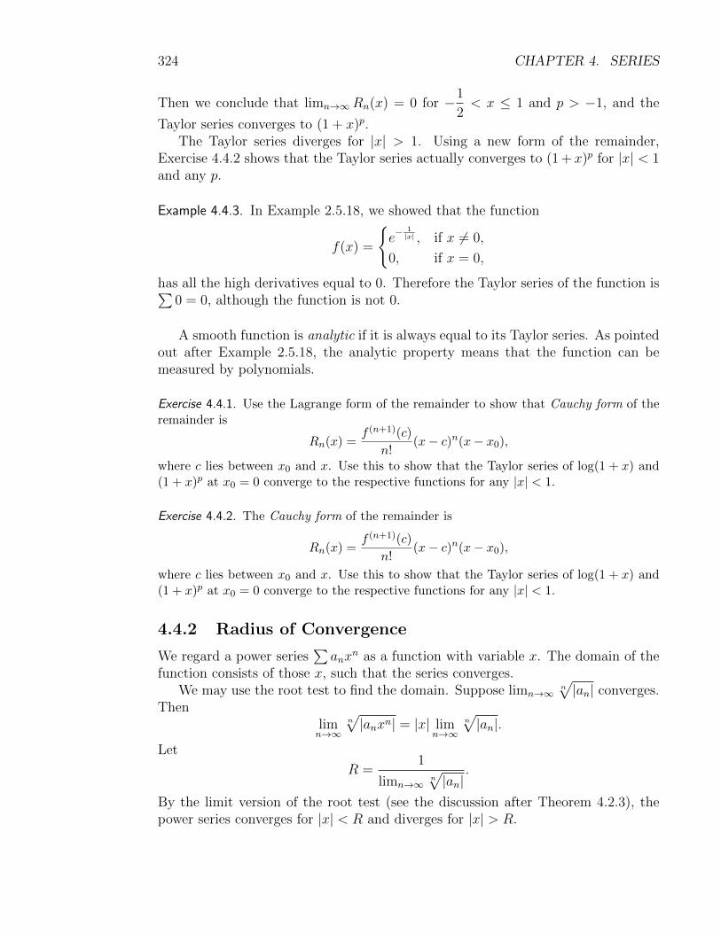
324 CHAPTER 4. SERIES
Then we conclude that limn→∞Rn(x) = 0 for −1
2< x ≤ 1 and p > −1, and the
Taylor series converges to (1 + x)p.The Taylor series diverges for |x| > 1. Using a new form of the remainder,
Exercise 4.4.2 shows that the Taylor series actually converges to (1 + x)p for |x| < 1and any p.
Example 4.4.3. In Example 2.5.18, we showed that the function
f(x) =
{e−
1|x| , if x 6= 0,
0, if x = 0,
has all the high derivatives equal to 0. Therefore the Taylor series of the function is∑0 = 0, although the function is not 0.
A smooth function is analytic if it is always equal to its Taylor series. As pointedout after Example 2.5.18, the analytic property means that the function can bemeasured by polynomials.
Exercise 4.4.1. Use the Lagrange form of the remainder to show that Cauchy form of theremainder is
Rn(x) =f (n+1)(c)
n!(x− c)n(x− x0),
where c lies between x0 and x. Use this to show that the Taylor series of log(1 + x) and(1 + x)p at x0 = 0 converge to the respective functions for any |x| < 1.
Exercise 4.4.2. The Cauchy form of the remainder is
Rn(x) =f (n+1)(c)
n!(x− c)n(x− x0),
where c lies between x0 and x. Use this to show that the Taylor series of log(1 + x) and(1 + x)p at x0 = 0 converge to the respective functions for any |x| < 1.
4.4.2 Radius of Convergence
We regard a power series∑anx
n as a function with variable x. The domain of thefunction consists of those x, such that the series converges.
We may use the root test to find the domain. Suppose limn→∞n√|an| converges.
Thenlimn→∞
n√|anxn| = |x| lim
n→∞n√|an|.
Let
R =1
limn→∞n√|an|
.
By the limit version of the root test (see the discussion after Theorem 4.2.3), thepower series converges for |x| < R and diverges for |x| > R.

4.4. POWER SERIES 325
Example 4.4.4. For the geometric series∑xn = 1+x+x2+· · · , we have limn→∞
n√|1| =
1. Therefore the geometric series converges for |x| < 1 and diverges for |x| > 1.Moreover, the series also diverges for |x| = 1.
For the Taylor series∑∞
n=0
(−1)n+1
nxn of log(1+x), we have limn→∞
n
√∣∣∣∣(−1)n+1
n
∣∣∣∣ =
limn→∞1n√n
= 1. Therefore the series converges for |x| < 1 and diverges for |x| > 1.
We also know that the series converges at x = 1 and diverges at x = −1.
Example 4.4.5. The series∑x2n has an = 1 for even n and an = 0 for odd n.
The sequence n√|an| diverges because it has two limits: limeven
n√|an| = 1 and
limoddn√|an| = 0.
On the other hand, as a function, we have∑x2n = f(x2), where f(x) =
∑xn
is the geometric series. Since the domain of f is |x| < 1, the domain of f(x2) is|x2| < 1, which is equivalent to |x| < 1. Therefore
∑x2n converges for |x| < 1 and
diverges for |x| > 1.
Theorem 4.4.1. For any power series∑anx
n, there is R ≥ 0, such that the seriesabsolutely converges for |x| < R and diverges for |x| > R.
Using the root test, we have proved the theorem in case limn→∞n√|an| converges.
Example 4.4.11 suggests that the theorem is true in general. The theorem is a con-sequence of the fact that, if
∑anr
n converges and |x| < |r|, then∑anx
n absolutelyconverges. Specifically, the convergence of
∑anr
n implies limn→∞ anrn = 0. This
further implies that |anrn| < 1 for sufficiently big n. Then for any fixed x satisfying|x| < |r|, we have
|anxn| = |anrn| ·∣∣∣xr
∣∣∣n ≤ ∣∣∣xr
∣∣∣n .Since
∣∣∣xr
∣∣∣ < 1 implies the convergence of∑∣∣∣x
r
∣∣∣n, by the comparison test, the series∑anx
n absolutely converges.The number R is the radius of convergence of power series. If R = 0, then the
power series converges only for x = 0. If R = +∞, then the power series convergesfor all x.
The same radius of convergence applies to∑an(x − x0)n. The power series
converges on (x0−R, x0 +R), and diverges on (−∞, x0−R) and on (x0 +R,+∞).We had the formula for radius in case n
√|an| converges. In general, the sequence
may have many possible limits (for various subsequences). Let the upper limitlim n√|an| be the maximum of all the possible limits. Then the radius is
R =1
limn→∞n√|an|
.
One can verify the formula for Example 4.4.11.

326 CHAPTER 4. SERIES
Example 4.4.6. For any p, we have limn→∞n√np = 1. Therefore the radius of conver-
gence for the power series∑npxn is 1. The example already appeared in Example
4.3.2.
Example 4.4.7. By limn→∞n√
2n + 3n = 3, the series∑
(2n + 3n)xn converges for
|x| < 1
3and diverges for |x| > 1
3. The series also diverges for |x| =
1
3because the
terms do not converge to 0.
We note that the radius of convergence is1
2for∑
2nxn and1
3for∑
3nxn. The
radius for the sum of the two series is the smaller one.
Example 4.4.8. By limn→∞n√nn = +∞, the series
∑nnxn diverges for all x 6= 0.
By limn→∞n
√1
nn= 0, the series
∑ (−1)n
nnxn converges for all x.
Example 4.4.9. In Example 4.2.9, we use the ratio test to show that the radius of
convergence of∑ (2n)!
(n!)2xn is
1
4. The idea can be used to show that the radius of
convergence for∑anx
n is R = limn→∞
∣∣∣∣ anan+1
∣∣∣∣, provided that the limit converges.
For example, by
limn→∞
np
(n+ 1)p=
(limn→∞
n
n+ 1
)p= 1,
the radius of convergence for∑npxn is 1. Moreover, the radius of convergence for
the Taylor series of ex is
limn→∞
1
n!1
(n+ 1)!
= limn→∞
(n+ 1) = +∞.
Example 4.4.10. The Bessel function of order 0 is
J0(x) =∞∑n=0
(−1)nx2n
22n(n!)2.
The radius of convergence is the square root of the radius of convergence of theseries
∞∑n=0
(−1)nxn
22n(n!)2.

4.4. POWER SERIES 327
By
limn→∞
∣∣∣∣∣∣∣∣(−1)n
22n(n!)2
(−1)n+1
22n+2((n+ 1)!)2
∣∣∣∣∣∣∣∣ = limn→∞
4(n+ 1)2 = +∞,
the later series converges for all x. Therefore the Bessel function is defined for all x.
Note that we cannot calculate limn→∞
∣∣∣∣ anan+1
∣∣∣∣ directly for the Bessel function. In
fact, the limit diverges.
Exercise 4.4.3. Suppose an can be divided into two subsequences an′ and an′′ . Suppose
limn′→∞n′√|an′ | = l′ and limn′′→∞
n′′√|an′′ | = l′′ converge. Prove that
1
max{l′, l′′}is the
radius of convergence for∑anx
n.
Exercise 4.4.4. Suppose limn→∞
∣∣∣∣ anan+1
∣∣∣∣ = R converges. Prove that R is the radius of
convergence for∑anx
n.
Exercise 4.4.5. Determine the radius of convergence.
1.∑
(−1)nxn
np.
2.∑np(x− 1)n.
3.∑np(2x− 1)n.
4.∑np(2x+ 3)n.
5.∑(
an
n+bn
n2
)xn.
6.∑ xn
an + bn.
7.∑n√nxn.
8.∑n!xn.
9.∑ (−1)n+1
√n!
xn.
10.∑ (n!)2
(2n)!xn.
11.∑ (3n)!
n!(2n)!xn.
12.∑an
2xn.
13.∑an
2xn
2.
14.∑
2nxn2−1.
15.∑
(2 + (−1)n)nxn.
16.∑ (2 + (−1)n)n
log nxn.
Exercise 4.4.6. Find the radius of convergence.
1.∑(
n+ 1
n
)nxn.
2.∑(
n+ 1
n
)n2
xn.
3.∑(
n+ a
n+ b
)n2
xn+2.
4.∑
(−1)n(n+ 1
n
)n2
xn.
5.∑
(−1)n(n+ 1
n
)n2
xn2.
6.∑(
an+ b
cn+ d
)nxn−2.
Exercise 4.4.7. Find the domain of the Bessel function of order 1
J1(x) =∞∑n=0
(−1)nx2n+1
n!(n+ 1)!22n+1.

328 CHAPTER 4. SERIES
Exercise 4.4.8. Find the domain of the Airy function
A(x) = 1 +x3
2 · 3+
x6
2 · 3 · 5 · 6+
x9
2 · 3 · 5 · 6 · 8 · 9+ · · · .
Exercise 4.4.9. Suppose the radii of convergence for∑anx
n and∑bnx
n are R and R′.What can you say about the radii of convergence for the following power series?∑
(an + bn)xn,∑
(an − bn)xn,∑
(−1)nanxn,
∑an(2x− 1)n,∑
anx2n,
∑anx
n+2,∑
a2nxn,
∑an+2x
n,∑anx
n2,∑
an2xn,∑
a2nx2n,
∑an2xn
2.
4.4.3 Function Defined by Power Series
Examples 2.5.18 and 4.4.3 suggest that if a function is the sum of a power series,then the function is particularly nice. In fact, the function should be nicer thanfunctions with derivatives of any order.
Because power series converge absolutely within the radius of convergence, byTheorem 4.3.5, we can multiply two power series together within the common radiusof convergence.
Theorem 4.4.2. Suppose f(x) =∑anx
n and g(x) =∑bnx
n have radii of conver-gence R and R′. Then for |x| < min{R,R′}, we have
f(x)g(x) =∑
cnxn, cn = a0bn + a1bn−1 + · · ·+ anb0.
The product should be the sum of aibjxi+j. We get the power series
∑cnx
n bygathering all the terms with power xn.
The power series can also be differentiated or integrated term by term withinthe radius of convergence.
Theorem 4.4.3. Suppose f(x) =∑∞
n=0 anxn for |x| < R. Then
f ′(x) =∞∑n=1
(anxn)′ = a1 + 2a2x+ 3a3x
2 + · · ·+ nanxn−1 + · · · ,
and ∫ x
0
f(t)dt =∞∑n=0
∫ x
0
antndt = a0x+
a1
2x2 +
a2
3x3 + · · ·+ an
n+ 1xn+1 + · · ·
for |x| < R.

4.4. POWER SERIES 329
Example 4.4.11. Taking the derivative of1
1− x=∑∞
n=0 xn, we get
1
(1− x)2= 1 + 2x+ 3x2 + 4x3 + · · ·+ nxn−1 + · · · ,
2
(1− x)3= 2 · 1 + 3 · 2x+ 4 · 3x2 + 5 · 4x3 + · · ·+ n(n− 1)xn−2 + · · · .
Therefore
12x+ 22x2 + · · ·+ n2xn + · · · =∞∑n=1
n2xn = x∞∑n=1
nxn−1 + x2
∞∑n=2
n(n− 1)xn−2
= x1
(1− x)2+ x2 2
(1− x)3=x(1 + x)
(1− x)3.
If we integrate instead, then we get
log(1− x) = −∫ x
0
dx
1− x= −x− x2
2− x3
3− · · · − xn
n!− · · · , for |x| < 1.
Substituting −x for x, we get the Taylor series of log(1 + x)
log(1 + x) = x− x2
2+x3
3− · · ·+ (−1)n+1x
n
n!+ · · · , for |x| < 1.
Note that in Example 4.4.1, by estimating the remainder, we were able to prove the
equality rigorously only for −1
2< x < 1. Here by using term wise integration, we
get the equality for all x within the radius of convergence.
Example 4.4.12. By integrating1
1 + x2=∑∞
n=0(−1)nx2n, we get the Taylor series of
arctanx
arctanx =∞∑n=0
(−1)n
2n+ 1x2n+1 = x− x
3
3+x5
5− x
7
7+ · · ·+ (−1)n
2n+ 1x2n+1 + · · · for |x| < 1.
Exercise 4.4.10. Use the product of power series to verify the identity sin 2x = 2 sinx cosx.
Exercise 4.4.11. Find Taylor series and determine the radius of convergence.
1.1
(x− 1)(x− 2), at 0.
2.√x, at x = 2.
3. sinx2, at 0.
4. sin2 x, at 0.
5. sinx, atπ
2.
6. sin 2x, atπ
2.
7. arcsinx, at 0.
8. arctanx, at 0.
9.
∫ x
0
sin t
tdt, at 0.

330 CHAPTER 4. SERIES
Exercise 4.4.12. Given the Taylor series∑∞
n=0 anxn of f(x), find the Taylor series of
f(x)
1 + x.
Exercise 4.4.13. Show that the function f(x) =∑∞
n=0
xn
(n!)2satisfies xf ′′ + f ′ − f = 0.
Exercise 4.4.14. Show that the Airy function in Exercise 4.4.8 satisfies f ′′ − xf = 0.
Exercise 4.4.15. Show that the Bessel functions in Example 4.4.10 and Exercise 4.4.7 satisfy
xJ ′′0 + J ′0 + xJ0 = 0, x2J ′′1 + xJ ′1 + (x2 − 1)J1 = 0.
A power series may or may not converge at the radius of convergence (i.e., at±R). If it converges, then the following gives the value of the sum.
Theorem 4.4.4. Suppose∑∞
n=0 anxn converges for |x| < R and x = R. Then∑∞
n=0 anRn = limx→R−
∑∞n=0 anx
n.
The theorem says that, if f(x) =∑∞
n=0 anxn is also defined at R, then f(x) is
left continuous at R. We also have the similar statement at the other end −R.
Example 4.4.13. By Examples 4.4.11 and 4.3.1, we know log(1 + x) =∑n
n=1
(−1)n+1
nxn
converges for |x| < 1, and the series converges at x = 1. Since log(1 + x) is continuous atx = 1, by Theorem 4.4.4, we get
n∑n=1
(−1)n+1
n= lim
x→1−
n∑n=1
(−1)n+1
nxn = lim
x→1−log(1 + x) = log(1 + 1) = log 2.
We computed the sum in Example 4.3.6 by another way.
Exercise 4.4.16. Find the sum. Discuss what happens at the radius of convergence.
1.∑∞
n=1 n2xn.
2.∑∞
n=1 n3xn.
3.∑∞
n=2
(x− 1)n
n(n− 1).
4.∑∞
n=1
xn
n(n+ 1)(n+ 2).
5.∑∞
n=0
x2n+1
2n+ 1.
6.∑∞
n=0
xn
2n+ 1.
Exercise 4.4.17. Find the sum. Discuss what happens at the radius of convergence.
1.∑∞
n=1(−1)nx2n+1
n!. 2.
∑∞n=1(−1)n
x2n
(2n+ 1)!. 3.
∑∞n=1
xn
2n(2n− 1)!.
Exercise 4.4.18. Find the Taylor series of the function and the radius of convergence. Thenexplain why the sum of the Taylor series is the given function.

4.5. FOURIER SERIES 331
1. arcsinx.
2.
∫ x
0
sin t
tdt.
3. arctanx.
4.
∫ x
0e−t
2dt.
5. log(x+√
1 + x2).
6.
∫ x
0
log(1− t)t
dt.
4.5 Fourier Series
If f(x+ p) = f(x) for all x and a constant p, then we say f(x) is a periodic functionof period p. For example, the functions sinx and cosx have period 2π, and tan xhas period π.
A periodic function of period p is also a periodic function of period kp for any
integer k. For example, cosnx and sinnx have the period p =2π
nas well as the
period np = 2π.
If f(x) has period p, then f(x+ a) still has period p, and f(ax) is periodic with
periodp
a.
A combination of periodic functions of the same period p is still periodic of periodp. For example, sinx + cos x, sin 3x cos2 x,
√2 sin2 x+ cos4 x are periodic of period
2π.
The Taylor series approximates a function near a point by linear combinationsof power functions. Similarly, we wish to approximate a periodic function by linearcombinations of simple periodic functions such as sine and cosine. Specifically, wewish a periodic function f(x) of period 2π to be approximated as
f(x) ∼ a0 +∞∑n=1
(an cosnx+ bn sinnx)
= a0 + a1 cosx+ b1 sinx+ a2 cos 2x+ b2 sin 2x+ · · · .
Note that there is no b0 because a0 = a0 cos 0x+ b0 sin 0x. Moreover, like the Taylorseries, we use ∼ instead of = to indicate that the equality is yet to be established.
The approximation of a periodic function by (linear combinations of) trigono-metric functions is not measured by the values at single points, but rather the overallapproximation in terms of the integral of the difference function. This means that wecan only expect that the sum of the trigonometric series to be equal to the function“almost everywhere”.
4.5.1 Fourier Coefficient
Let f(x) be a periodic function of period 2π. Our first problem is to find thecoefficients an and bn in the trigonometric series. By Exercise 3.1.6, the trigonometric

332 CHAPTER 4. SERIES
functions are “orthogonal” in the sense that∫ 2π
0
cosmx sinnxdx = 0;
∫ 2π
0
cosmx cosnxdx =
0, if m 6= n,
π, if m = n 6= 0,
2π, if m = n = 0;∫ 2π
0
sinmx sinnxdx =
{0, if m 6= n or m = n = 0,
π, if m = n 6= 0.
We expect the sum of the trigonometric series to be equal to f(x) as far as integra-tions are concerned. We also assume that the integration of infinite series can becalculated term by term. Then we get
∫ 2π
0
f(x) cosnxdx = a0
∫ 2π
0
cosnxdx+∞∑k=1
am
∫ 2π
0
cosmx cosnxdx
+∞∑k=1
bm
∫ 2π
0
sinmx cosnxdx =
{πan, if n 6= 0,
2πa0, if n = 0;∫ 2π
0
f(x) sinnxdx = a0
∫ 2π
0
sinnxdx+∞∑m=1
am
∫ 2π
0
cosmx sinnxdx
+∞∑m=1
bm
∫ 2π
0
sinmx sinnxdx = πbn.
Definition 4.5.1. The Fourier series of a periodic function f(x) of period 2π is
f(x) ∼ a0 +∞∑n=1
(an cosnx+ bn sinnx),
with the Fourier coefficients
a0 =1
2π
∫ 2π
0
f(x)dx,
an =1
π
∫ 2π
0
f(x) cosnxdx, n 6= 0,
bn =1
π
∫ 2π
0
f(x) sinnxdx, n 6= 0.

4.5. FOURIER SERIES 333
Example 4.5.1. Similar to Example 2.5.1, by
sin4 x =1
4(1− cos 2x)2 =
1
4
(1− 2 cos 2x+
1
2(1− cos 4x)
)=
3
8− 1
2cos 2x+
1
8cos 4x,
the right side is the Fourier series of sin4 x. The coefficients give∫ 2π
0
sin4 xdx =3π
4,
∫ 2π
0
sin4 x cos 2xdx = −π2,
∫ 2π
0
sin4 x cos 4xdx =π
8.
Example 4.5.2. A periodic function is determined by its value on one interval ofperiod length. For example, if f(x) is a periodic function of period 2π and satisfies
f(x) =
{1, if 0 ≤ x < a,
0, if a ≤ x < 2π,
then
f(x) =
{0, if 2kπ ≤ x < 2kπ + a,
1, if 2kπ + a ≤ x < 2(k + 1)π.
−4π 4π−2π 2πa
The Fourier coefficients are
a0 =1
2π
∫ a
0
1dx =a
2π,
an =1
π
∫ a
0
cosnxdx =sinna
nπ,
bn =1
π
∫ a
0
sinnxdx =1− cosna
nπ.
and the Fourier series is
f(x) ∼ a
2π+∞∑n=1
1
nπ(sinna cosnx+ (1− cosna) sinnx).
Example 4.5.3. Let f(x) be the even periodic function of period 2π satisfying
f(x) =
{1, if |x| ≤ a,
0, if a < |x| ≤ π.

334 CHAPTER 4. SERIES
−4π 4π−2π 2π−π πa
We have
a0 =1
2π
∫ 2π
0
f(x)dx =1
2π
∫ π
−πf(x)dx =
1
π
∫ π
0
f(x)dx =1
π
∫ a
0
1dx =a
π,
an =1
π
∫ 2π
0
f(x) cosnxdx =2
π
∫ π
0
f(x) cosnxdx =2
π
∫ a
0
cosnxdx =2a
nπ.
The calculation used the fact that
∫ p
0
f(x)dx =
∫ a+p
a
f(x)dx for any periodic func-
tion of period p. We may also calculate bn and find bn = 0. In fact, for even function,we expect that all the odd terms bn sinnx to vanish.
Exercise 4.5.1. Suppose f(x) is an even periodic function of period 2π. Prove that
a0 =1
π
∫ π
0f(x)dx, an =
2
π
∫ π
0f(x) cosnxdx, bn = 0.
Exercise 4.5.2. Suppose f(x) is an odd periodic function of period 2π. Prove that
a0 = an = 0, bn =2
π
∫ π
0f(x) sinnxdx.
Exercise 4.5.3. Extend f(x) on(
0,π
2
)to a periodic function of period 2π, such that its
Fourier series is of the form∑∞
n=1 an cos(2n− 1)x? How about∑∞
n=1 bn sin(2n− 1)x?
Exercise 4.5.4. Given the Fourier series of f(x) and g(x), what is the Fourier series ofaf(x) + bg(x)? Use the idea and Example 4.5.2 to find the Fourier series of the periodicfunction f(x) of period 2π satisfying
f(x) =
{1, if a ≤ x < b,
0, if 0 ≤ x < a or b ≤ x < 2π.
Exercise 4.5.5. Suppose f(x) is a periodic function of period 2π. What is the relationbetween the Fourier series of f(x) and f(x+a)? Use the idea and Example 4.5.3 to deriveExample 4.5.2.
A periodic function f(x) of period p may be converted to a periodic function
f( p
2πx)
of period 2π. Then the Fourier series of f( p
2πx)
gives the Fourier series
of f(x). Alternatively, the basic periodic functions cosnx and sinnx of period 2π

4.5. FOURIER SERIES 335
give the basic periodic functions cos2nπ
px and sin
2nπ
px of period p, and we expect
the Fourier series of f(x) to be
f(x) ∼ a0 +∞∑n=1
(an cos
2nπ
px+ bn sin
2nπ
px
).
By an argument similar to the case of period 2π, we get the Fourier coefficients
a0 =1
p
∫ p
0
f(x)dx,
an =2
p
∫ p
0
f(x) cos2nπ
pxdx, n 6= 0,
bn =2
p
∫ p
0
f(x) sin2nπ
pxdx, n 6= 0.
Exercise 4.5.6. Suppose f(x) is a periodic function of period p.
1. Write down the Fourier series for f( p
2πx)
, together with the formulae for its coef-
ficients.
2. Convert the first part to statements about the original f(x).
Exercise 4.5.7. Use Example 4.5.2 to derive the Fourier series of the periodic function ofperiod 1 satisfying
f(x) =
{1, if 0 ≤ x < a,
0, if a ≤ x < 1.
Exercise 4.5.8. Derive the formulae for the Fourier coefficients of periodic even or oddfunctions of period p, similar to Exercises 4.5.1 and 4.5.2.
Example 4.5.4. The function x on (0, 1) extends to a periodic function of period 1
f(x) = x− k, k < x < k + 1.
−4 −3 −2 −1 1 2 3 4
Note that we do not care about the value at the integer points because it does

336 CHAPTER 4. SERIES
not affect the Fourier coefficients, which are
a0 =1
1
∫ 1
0
xdx =1
2,
an =2
1
∫ 1
0
x cos 2nπxdx =1
nπ
∫ 1
0
xd sin 2nπx = − 1
nπ
∫ 1
0
sin 2nπxdx = 0,
bn =2
1
∫ 1
0
x sin 2nπxdx = − 1
nπ
∫ 1
0
xd cos 2nπx
= − 1
nπ
(1−
∫ 1
0
cos 2nπxdx
)= − 1
nπ.
We note that the reason for an = 0 for n 6= 0 is that f(x)− 1
2is an odd function.
The Fourier series is
x ∼ 1
2− 1
π
∞∑n=1
1
nsin 2nπx, x ∈ (0, 1).
We indicate x ∈ (0, 1) because the function equals x only on the interval. Thefunction is x− 1 instead of x on the interval (1, 2).
Example 4.5.5. The function x on (0, 1) extends to an even periodic function ofperiod 2
f(x) = |x− 2k|, 2k − 1 < x < 2k + 1.
This is also the extension of the function |x| on (−1, 1) to a periodic function ofperiod 2.
−4 −3 −2 −1 1 2 3 4
Using Exercises 4.5.1 and 4.5.8, we get bn = 0 and
a0 =2
2
∫ 1
0
f(x)dx =
∫ 1
0
xdx =1
2,
an =2
1
∫ 1
0
f(x) cosnπxdx = 2
∫ 1
0
x cosnπxdx =
−4
n2π2, if n is odd,
0, if n is even.
Replacing n by 2n+ 1, the Fourier series is
|x| ∼ 1
2− 4
π2
∞∑n=0
1
(2n+ 1)2cos(2n+ 1)πx, x ∈ (−1, 1).

4.5. FOURIER SERIES 337
We may also extend the function to an odd periodic function of period 2. Thisis also the extension of the function x on (−1, 1) to a periodic function of period 2.The Fourier coefficients an = 0 for the odd function, and
bn = 2
∫ 1
0
x sinnπxdx =(−1)n+12
nπ.
The Fourier series is
x ∼∞∑n=1
(−1)n+12
nπsinnπx, x ∈ (−1, 1).
−4 −3 −2 −1 1 2 3 4
Example 4.5.6. Let f(x) be the periodic function of period 1 extending the functionx2 on (0, 1). Then
a0 =
∫ 1
0
x2dx =1
3,
an = 2
∫ 1
0
x2 cos 2nπxdx =1
n2π2,
bn = 2
∫ 1
0
x2 sin 2nπxdx = − 1
nπ.
The Fourier series is
x2 ∼ 1
3+∞∑n=1
(1
n2π2cos 2nπx− 1
nπsin 2nπx
), x ∈ (0, 1).
−4 −3 −2 −1 1 2 3 4
Exercise 4.5.9. The periodic function is given on one interval of period length. Find theFourier series.

338 CHAPTER 4. SERIES
1. sin2 x on (−π, π).
2. sinx on (0, π).
3. | sinx| on (0, 2π).
4. sinx on (0, p).
5. cosx on (0, p).
6. |x| on (−p, p).
7. x on (a, b).
8. x sinx on (−π, π).
9. ex on (0, 1).
Exercise 4.5.10. Use the Fourier coefficient to calculate the integral.
1.
∫ π
0sin2 x cos 2xdx.
2.
∫ 2π
0sin6 xdx.
3.
∫ 2π
0sinx cos 2x sin 3xdx.
4.
∫ 2π
0sinx cos 2x cos 3xdx.
5.
∫ 2π
0sin3 x sin 3xdx.
6.
∫ 2π
0sin3 x cos 3xdx.
Exercise 4.5.11. Write the formula for the Fourier coefficients of the even periodic (ofperiod 2p) extension of a function f(x) on (0, p). What about the odd extension?
Exercise 4.5.12. Extend the function on (0, p) to even and odd functions of period 2p andcompute the Fourier series.
1. x2 on (0, 1). 2. sinx on (0, π). 3. cosx on (0, p).
Exercise 4.5.13. Given the Fourier series of functions f(x) and g(x) of period p. Find theFourier series of the following periodic functions.
1. f(ax).
2. f(x) cos2πx
p.
3. f(x) sin2πx
p.
4.1
2h
∫ x+h
x−hf(t)dt.
5.1
h
∫ x+h
xf(t)dt.
6.
∫ p
0f(t)g(x− t)dt.
Exercise 4.5.14. Use Examples 4.5.4 and 4.5.5 to find the Fourier series.
1. x on (0, p).
2. −x on (−p, 0).
3. |x| on (−p, p).
4. 0 on (−1, 0) and x on (0, 1).
5. ax on (−1, 0) and bx on (0, 1).
6. ax on (−p, 0) and bx on (0, p).
4.5.2 Complex Form of Fourier Series
The sine and cosine functions are related to the exponential function via the use ofcomplex numbers
eix = cosx+ i sinx, cosx =eix + e−ix
2, sinx =
eix − e−ix
2i, i =
√−1.

4.5. FOURIER SERIES 339
Correspondingly, the Fourier series may be rewritten
f(x) =∞∑
n=−∞
cneinx, c0 = a0, cn =
an − ibn2
, c−n =an + ibn
2,
where complex Fourier coefficients are
cn =1
2π
∫ 2π
0
f(x)e−inxdx.
In this course, f(x) is a real valued function, and an, bn are real numbers. There-fore c−ne
i(−n)x is the complex conjugation of cneinx, and the usual Fourier series is
given bya0 = c0, an cosnx+ bn sinnx = 2Re(cne
inx).
Example 4.5.7. For the function in Example 4.5.2, the complex Fourier coefficient is
c0 =1
2π
∫ a
0
dx =a
2π,
cn =1
2π
∫ a
0
e−inxdx =1
−2inπe−inx|a0 =
i
2nπ(e−ina − 1).
The complex Fourier series is
f(x) ∼ a
2π+∑n6=0
i
2nπ(e−ina − 1)einx, x ∈ (0, 2π).
By
2Re
(i
2nπ(e−ina − 1)einx
)= Re
(i
nπ((cosna− 1)− i sinna)(cosnx+ i sinnx)
)=
1
nπ(sinna cosnx− (cosna− 1) sinnx),
we recover the Fourier series in terms of trigonometric functions in Example 4.5.2.
Example 4.5.8. Consider the periodic function of period 2π given by ex on (0, 2π).The complex Fourier coefficient is (recall that e2ikπ = 1)
cn =1
2π
∫ 2π
0
exe−inxdx =1
2π(1− in)e(1−in)x|2π0 =
e2π − 1
2nπ(1− in).
The complex Fourier series is
ex ∼ e2π − 1
2π
∞∑n=−∞
1
1− ineinx, x ∈ (0, 2π).

340 CHAPTER 4. SERIES
By
Re
(1
1− ineinx)
= Re
(1 + in
1 + n2(cosnx+ i sinnx)
)=
cosnx− n sinnx
1 + n2,
we get the Fourier series in terms of trigonometric functions
ex ∼ e2π − 1
π
(1
2+∞∑n=1
cosnx− n sinnx
1 + n2
), x ∈ (0, 2π).
By changing x to 2πx, we get the Fourier series for the periodic function of period1 given by e2πx on (0, 1)
e2πx ∼ e2π − 1
π
(1
2+∞∑n=1
cos 2nπx− n sin 2nπx
1 + n2
), x ∈ (0, 1).
Example 4.5.9. Consider the function f(x) =a sinx
1− 2a cosx+ a2, with |a| < 1. We
rewrite the function and take the Taylor expansion in terms of einx = zn, z = eix,
a sinx
1− 2a cosx+ a2=
aeix − e−ix
2i
1− 2aeix + e−ix
2+ a2
=a
2i
eix − e−ix
(1− aeix)(1− ae−ix)=
1
2i
(1
1− aeix− 1
1− ae−ix
)=
1
2i
(∞∑n=0
(aeix)n −∞∑n=0
(ae−ix)n
)=
1
2i
∑n6=0
a|n|einx
=1
2i
∞∑n=1
an(einx − e−inx) =∞∑n=1
an sinnx.
Note that we have geometric series because |aeix| = |ae−ix| = |a| < 1. Moreover,the Fourier series is actually equal to the function. The example also shows theconnection between the Fourier series and the power series.
Exercise 4.5.15. Find the complex form of the Fourier series of ax on (0, 2π). Then by
taking a = e1
2π , derive the Fourier series of the function ex on (0, 1).
Exercise 4.5.16. Find the complex form of the Fourier series of eix2 on (0, 2π). Then derive
the Fourier series of cosx and sinx on (0, π) by taking the real and imaginary parts.
Exercise 4.5.17. What is the complex form of the Fourier series for a periodic function ofperiod p?
Exercise 4.5.18. Find complex form of Fourier series.

4.5. FOURIER SERIES 341
1. sin2 x on (−π, π).
2. eix on (0, p).
3. |x| on (−p, p).
4. x2 on (0, 1).
5. x sinx on (−π, π).
6. x cosx on (−π, π).
Exercise 4.5.19. Find Fourier series, where |a| < 1.
1.1− a cosx
1− 2a cosx+ a2. 2.
1− a2
1− 2a cosx+ a2. 3. log(1− 2a cosx+ a2).
4.5.3 Derivative and Integration of Fourier Series
The derivative of a periodic function is still periodic. We may use f(p) = f(0)(which is the periodic property) and the integration by parts to compute the Fouriercoefficients An, Bn of f ′(x)
A0 =1
p
∫ p
0
f ′(x)dx =1
p(f(p)− f(0)) = 0,
An =2
p
∫ p
0
f ′(x) cos2nπ
pxdx =
2
p
∫ p
0
cos2nπ
pxdf(x)
=2
p
(f(p)− f(0) +
∫ p
0
f(x)2nπ
psin
2nπ
pxdx
)=
2nπ
pbn,
Bn =2
p
∫ p
0
f ′(x) sin2nπ
pxdx =
2
p
∫ p
0
sin2nπ
pxdf(x)
= −2
p
∫ p
0
f(x)2nπ
pcos
2nπ
pxdx = −2nπ
pan.
This shows that we may differentiate the Fourier series term by term.
Proposition 4.5.2. Suppose f(x) is a periodic function of period p that is continuousand piecewise continuously differentiable. If the Fourier coefficients of f(x) arean, bn, then the Fourier series of f ′(x) is
f ′(x) ∼ 2π
p
∞∑n=1
n
(bn cos
2nπ
px− an sin
2nπ
px
).
The integration F (x) =
∫ x
0
f(t)dt of a periodic function of period p is still
periodic if a0 =1
p
∫ p
0
f(x)dx = 0. Then for n 6= 0, the other Fourier coefficients of

342 CHAPTER 4. SERIES
F (x) are
An =2
p
∫ p
0
F (x) cos2nπ
pxdx =
1
nπ
∫ p
0
F (x)d sin2nπ
px
= − 1
nπ
∫ p
0
f(x) sin2nπ
pxdx = − p
2nπbn,
Bn =2
p
∫ p
0
F (x) sin2nπ
pxdx = − 1
nπ
∫ p
0
F (x)d cos2nπ
px
= − 1
nπ
(∫ p
0
f(x)dx−∫ p
0
f(x) cos2nπ
pxdx
)=
p
2nπan.
The 0-th coefficient is
A0 =1
p
∫ p
0
F (x)dx =1
p
(xF (x)|x=p
x=0 −∫ p
0
xf(x)dx
)= −1
p
∫ p
0
xf(x)dx.
This shows that, in case a0 = 0, we may almost integrate the Fourier series term byterm.
Proposition 4.5.3. Suppose f(x) is a periodic function of period p. If the Fourier co-
efficients of f(x) are an, bn and a0 = 0, then the Fourier series of F (x) =
∫ x
0
f(t)dt
is ∫ x
0
f(t)dt ∼ A0 +p
2π
∞∑n=1
1
n
(−bn cos
2nπ
px+ an sin
2nπ
px
).
Example 4.5.10. In Example 4.5.4, we found the Fourier series
x ∼ 1
2− 1
π
∞∑n=1
1
nsin 2nπx, x ∈ (0, 1).
We wish to integrate to get the Fourier series of x2 on (0, 1). However, to satisfy
the condition of Proposition 4.5.3, we should consider the Fourier series of x − 1
2,
which has vanishing 0-th coefficient. Then F (x) =
∫ x
0
(t− 1
2
)dt =
1
2x2 − 1
2x has
Fourier series
1
2x2 − 1
2x ∼ − 1
12+
1
2π2
∞∑n=1
1
n2cos 2nπx, x ∈ (0, 1).
Here the 0-th coefficient is
A0 = −∫ 1
0
x
(x− 1
2
)dx = − 1
12.

4.5. FOURIER SERIES 343
Then the Fourier series of x2 = 2
(1
2x2 − 1
2x
)+ x on (0, 1) is
x2 ∼ 2
(− 1
12+
1
2π2
∞∑n=1
1
n2cos 2n
)+
(1
2− 1
π
∞∑n=1
1
nsin 2nπx
)
=1
3+∞∑n=1
(1
n2π2cos 2nπx− 1
nπsin 2nπx
), x ∈ (0, 1).
We obtained this Fourier series in Example 4.5.6 by direct computation.
Exercise 4.5.20. Derive the Fourier series of x3 on (0, 1) from the Fourier series of x2.
Exercise 4.5.21. Derive the Fourier series of |x| on (−1, 1) from the Fourier series of itsderivative.
Exercise 4.5.22. Suppose f(x) is continuously differentiable on [0, p], with perhaps differentf(0+) and f(p−). Then we can extend both f(x) and f ′(x) to periodic functions of periodp. If the Fourier coefficients of the extended f(x) are an, bn, prove that
f ′(x) ∼ f(p−)− f(0+)
p+
2
p
∞∑n=1
((f(p−)− f(0+) + nπbn) cos
2nπ
px+ nπan sin
2nπ
px
).
4.5.4 Sum of Fourier Series
Like the Taylor series, the Fourier series may not always converge to the function.The following is one good case when the Fourier series converges.
Theorem 4.5.4. Suppose f(x) is a periodic function. If f(x) has one sided limitsf(x−0 ) and f(x+
0 ) at x0, and there is M , such that
x < x0 and close to x0 =⇒ |f(x)− f(x−0 )| ≤M |x− x0|,
andx > x0 and close to x0 =⇒ |f(x)− f(x+
0 )| ≤M |x− x0|.
Then the Fourier series of f(x) converges tof(x+
0 ) + f(x−0 )
2at x = x0.
The condition means that the value of f(x) lies in two “corners” on the two sidesof x0.
Example 4.5.11. In Example 4.5.4, we find the Fourier series of x on (0, 1). The functionsatisfies the condition of Theorem 4.5.4 at x0 = 0. We conclude that
0 + 1
2=f(0−) + f(0+)
2=
1
2− 1
π
∞∑n=1
1
nsin 2nπ0.

344 CHAPTER 4. SERIES
x0
f(x−0 )
f(x+0 )
Figure 4.5.1: Condition for the convergence of Fourier series.
This is trivially true. We get similar trivial equalities at x0 = 1 and x0 =1
2.
If we take x0 =1
3, then
1
3=
1
2− 1
π
∞∑k=1
(1
3k + 1sin
2(3k + 1)π
3+
1
3k + 2sin
2(3k + 2)π
3+
1
3k + 3sin
2(3k + 3)π
3
)
=1
2− 1
π
∞∑k=1
(1
3k + 1
√3
2− 1
3k + 2
√3
2
).
This means that
1− 1
2+
1
4− 1
5+
1
7− 1
8+
1
10− 1
11+
1
13− 1
14+ · · · = π
3√
3.
Similarly, by evaluating the Fourier series at x0 =1
4and x0 =
1
8, we get
1− 1
3+
1
5− 1
7+
1
9− 1
11+
1
13− 1
15+
1
17− 1
19+ · · · = π
4,
1 +1
3− 1
5− 1
7+
1
9+
1
11− 1
13− 1
15+
1
17+
1
19− · · · = π
2√
2.
Example 4.5.12. The periodic function of period 2 given by |x| on (−1, 1) satisfies thecondition of Theorem 4.5.4 everywhere. Evaluating the Fourier series in Example 4.5.4 atx = 0, we get
0 =1
2− 4
π2
∞∑n=0
1
(2n+ 1)2.
This means that∞∑n=0
1
(2n+ 1)2= 1 +
1
32+
1
52+
1
72+ · · · = π2
8.
If the sum also includes the even terms, then we have
∞∑n=1
1
n2=∞∑n=0
1
(2n+ 1)2+∞∑n=1
1
(2n)2=∞∑n=0
1
(2n+ 1)2+
1
4
∞∑n=1
1
n2.

4.5. FOURIER SERIES 345
0 1
Figure 4.5.2: Partial sums of the Fourier series for x on (0, 1).
Therefore∞∑n=1
1
n2= 1 +
1
22+
1
32+
1
42+ · · · = 4
3
∞∑n=0
1
(2n+ 1)2=π2
6.
If we evaluate at x =1
4, then we get
1
4=
1
2− 4√
2π2
(1
12+
1
32− 1
52− 1
72+
1
92+
1
112− 1
132− 1
152+ · · ·
).
Combined with the sum above, we get
1
12+
1
32+
1
92+
1
112+
1
172+
1
192+ · · · =
(1
12+
1
16√
2
)π2,
1
52+
1
72+
1
132+
1
152+
1
212+
1
232+ · · · =
(1
12− 1
16√
2
)π2.
Exercise 4.5.23. Use the Fourier series of x2 on (0, 1) to compute∑∞
n=1
1
n2.
Exercise 4.5.24. Use the Fourier series of x2 on (−1, 1) to get the Fourier series of x3 and
x4 on (−1, 1). Then evaluate the Fourier series of x4 to get∑∞
n=1
1
n4.
4.5.5 Parseval’s Identity
In Example 4.5.1, we had the Fourier series
sin4 x =3
8− 1
2cos 2x+
1
8cos 4x.
Then ∫ 2π
0
sin8 xdx =
∫ 2π
0
(3
8− 1
2cos 2x+
1
8cos 4x
)2
dx.

346 CHAPTER 4. SERIES
We may expand the square on the right. We get square terms such as1
22cos2 2x
and cross terms such as 21
2· 1
8cos 2x cos 4x. The square term has nonzero integral∫ 2π
0
cos2 2xdx = π.
The cross terms has vanishing integral∫ 2π
0
cos 2x cos 4xdx = 0.
Therefore ∫ 2π
0
sin8 xdx =
(3
8
)2
2π +
(1
2
)2
π +
(1
8
)2
π =35
64π.
The idea (which is essentially Pythagorean theorem) leads to the following formula.
Theorem 4.5.5 (Parseval’s Identity). Suppose f(x) is a periodic function of periodp. Then its Fourier coefficients satisfy
2a20 +
∞∑n=1
(a2n + b2
n) =2
p
∫ p
0
|f(x)|2dx.
The identity means that the Fourier series, considered as a conversion betweenperiodic functions and sequences of numbers, preserves the “Euclidean length”. Thecomplex form of Parseval’s identity is
∞∑n=−∞
|cn|2 =1
2π
∫ 2π
0
|f(x)|2dx.
Example 4.5.13. Applying Parseval’s identity to the Fourier series of x on (0, 1), weget
2 +∞∑n=1
1
n2π2= 2
∫ 1
0
x2dx =2
3.
This is the same as1
12+
1
22+
1
32+
1
42+ · · · = π2
6.
Applying the identity to the Fourier series of x2 on (0, 1), we get
2
9+∞∑n=1
1
n4π4+∞∑n=1
1
n2π2= 2
∫ 1
0
x4dx =2
5.
Using∑∞
n=1
1
n2=π2
6, we get
1
14+
1
24+
1
34+
1
44+ · · · = π4
90.

4.5. FOURIER SERIES 347
Example 4.5.14. Applying Parseval’s identity to the complex form of the Fourierseries of ex on (0, 2π) in Example 4.5.8, we get
(e2π − 1)2
4π2
∞∑n=−∞
1
1 + n2=
1
2π
∫ 2π
0
e2xdx =e4π − 1
4π.
The equality leads to
1 + 2∞∑n=1
1
1 + n2=e2π + 1
e2π − 1π,
or∞∑n=1
1
1 + n2=
1
2+
1
5+
1
10+
1
17+
1
26+ · · · = π(e2π + 1)
2(e2π − 1)− 1
2.
Exercise 4.5.25. Apply Parseval’s identity to the Fourier series in Example 4.5.2 to find∑∞n=1
sin2 na
n2and
∑∞n=1
cos2 na
n2.
Exercise 4.5.26. Apply Parseval’s identiy to the Fourier series of x3 and x4 on (0, 1) to find∑∞n=1
1
n6and
∑∞n=1
1
n8.
Exercise 4.5.27. Find∑∞
n=1
1
1 + n2by evaluating the Fourier series in Example 4.5.8.