Calculus 3.pdf
363
-
Upload
khangminh22 -
Category
Documents
-
view
0 -
download
0
Transcript of Calculus 3.pdf


Copyright 1985 Springer-Verlag. All rights reserved
Geometry Formulas
Area of rectangle A = lw
circle A = 7Tr2
triangle A = ~ bh
Surface Area of sphere A = 47Tr2
cylinder A = 27Trh
Volume of box V = lwh
sphere V = .t 7Tr3
cylinder V = 7Tr2h
cone V = 1 (area of base) X (height)
Trigonometric Identities
Pythagorean
cos28 + sin28 = 1, I + tan28 = sec28, cot28 + I = csc28
Parity
sin( - (}) = - sin 8, cos( - (}) = cos 8, tan( - (}) = - tan(}
csc( - 8) = - csc 8, sec( - (}) = sec 8, cot( - (}) = - cot(}
Co-relations
cos(}= sin( 1- (} ), csc (}=sec( 1- (}),cot(}= tan( 1- (}) Addition formulas
sin((} + cp) = sin (}cos cf> + cos ti sin cf>
sin(8 - cf>)= sin8coscp- cos8sincp
cos((} + cf>) = cos (} cos cf> - sin (} sin cf>
cos((} - cf>) = cos(} cos cf> + sin(} sin cp
(tan (} + tan cf>) tan(8 +cf>)= ---
( I - tan (} tan cf>)
(tan (} - tan cp) tan(8-cp)= ----
( I + tan (} tan cf>)
Double-angle formulas
sin 28 = 2 sin (} cos (}
cos 28 = cos28 - sin28 = 2 cos28 - I = I - 2 sin20
tan 28 = 2 tan 8 (I - tan28)
Half-angle formulas
·28 l-cos8 sm 2 = 2
cos2 (j_ = I + cos 8 2 2
tan (j_ = sin(} 2 I +cos 8
Product formulas
or
or
I - cos(} sin8
sin2(} = I - cos 28 2
cos2(} = I + cos 28 2
or tan(}= I - cos28 sin28
sin (} sin cf> = i [cos((} - cf>) - cos((} + cf>)]
cos8coscp = i [cos((}+ cf>)+ cos(8 - cp)]
sin8coscp = i [sin((}+ cp) +sin((} - cp)]

Copyright 1985 Springer-Verlag. All rights reserved
d(au) du 1. ~ =adx
d(u + v - w) du dv dw 2· dx = dx + dx - dx
d(uv) dv du 3· ~ = u dx + v dx
d(u/v) v(du/dx)- u(dv/dx) 4. -d-- = 2
x v
5 d(un) =nun-I du · dx dx
6 d(uv) = vuv-l du +uv(lnu)dv 'dx dx dx
7 d(eu) =eudu · dx dx
d(eau) du 8 -- = aeau_
· dx dx
9. dau = au(lna) du dx dx
d(lnu) l du 10· -----;JX = u dx
d(logau) _ l du l l. dx - u (In a) dx
dsinu = cosu du 12· dx dx
13 dcosu = -sinu du · dx dx
14 d tan u = sec2u du · dx dx
15 dcotu = -csc2u du · dx dx
16 dsecu = tanusecu du · dx dx
17. d~:u = -(cotu)(cscu) :~
dsin- 1u 18. dx
l du
~dx
Derivatives
d cos - 1u - l du 19· dx d ~x
20. dtan- 1u du
dx = l + u2 dx
21. d cot- 1u -1 du
dx = l + u2 dx
22. dsec- 1u du
dx u~ dx
dcsc- 1u = -1 du 23· dx ~ -d uyu2 - l x
24 dsinhu = coshu du · dx dx
dcoshu · h du 25. dX = sm u dx
26 d tanh u = sech2u du · dx dx
27. dc~~hu = -(csch2u) :~
28. d s~~h u = -(sech u)(tanh u) :~
29. dc~~hu = -(cschu)(cothu) :~
d sinh- 1u du 30. dx ~ dx
d cosh- 1u l du 31. dx ~ dx
dtanh- 1u du 32. =--dx l - u2 dx
d coth- 1u du 33. dx = 1 _ u2 dx
dsech- 1u -1 du 34. dx u~ dx
dcsch- 1u = -1 du 35. dx lul{l+7
dx
Continued on overleaf.

Copyright 1985 Springer-Verlag. All rights reserved
A Brief Table of Integrals
(An arbitrary constant may be added to each integral.)
1. Jx"dx= - 1-xn+l (n"/' -1) n + 1
2. J ± dx = ln[x[
3. Jex dx =ex
4. Jaxdx= ~ Ina
5. Jsinxdx = -cosx
6. J cosx dx = sinx
7. Jtanxdx = -ln[cosx[
8. J cotxdx = ln[sinx[
9. Jsecxdx=ln[secx+tanx[
= Injtan( ix+ i?T)I 10. J cscxdx = ln[cscx - cotx[
= ln[tanix[
11. Jsin- 1 ~ dx = xsin- 1 ~ +..ja2 - x 2 a a
(a> 0)
12. Jcos- 1 ~ dx = xcos- 1 ~ -../a2 - x 2 (a> 0) a a
13.Jtan- 1 ~dx=xtan- 1 ~ -~ln(a2 +x2) (a>O) a a 2
14. Jsin2mxdx = 2~ (mx - sinmxcosmx)
15. J cos2mxdx = 2~ (mx + sinmxcosmx)
16. J sec2x dx = tan x
17. J csc2x dx = -cotx
J . n-1 n - 1 J 2 18. sinnxdx = - sm :cosx + -n- sinn- xdx
19. Jcosnxdx= cosn-~xsinx + n~ 1 Jcosn-2xdx
J tann-lx J 20. tan"x dx = ---;:;-=-} - tann- 2x dx (n "/' l)
J cotn-lx J 21. cotnx dx = - ---;:;-=-} - cotn - 2x dx (n °=!= 1)
22 J n d _ tan x secn- 2x + n - 2 J n-2 d . sec x x - n _ 1
n _ 1
sec x x (n "/' 1)
23 J n d cotx cscn- 2x . csc x x = - n _ l + -- cscn- x dx n -2 J 2 n - 1
(n "/' 1)
24. J sinh x dx = cosh x
25. J cosh x dx = sinh x
26. J tanhx dx = ln[coshx[
27. J coth x dx = ln[sinh x[
28. Jsechxdx=tan- 1(sinhx)
This table is continued on the endpapers at the back.

Copyright 1985 Springer-Verlag. All rights reserved
Springer New York Berlin Heidelberg Barcelona Hong Kong London Milan Paris Singapore Tokyo
Undergraduate Texts in Mathematics
Editors S. Axler
F.W. Gehring K.A. Ribet

Copyright 1985 Springer-Verlag. All rights reserved
Undergraduate Texts in Mathematics
Abbott: Understanding Analysis. Anglin: Mathematics: A Concise History
and Philosophy. Readings in Mathematics.
Anglin/Lambek: The Heritage of Thales. Readings in Mathematics.
Apostol: Introduction to Analytic Number Theory. Second edition.
Armstrong: Basic Topology. Armstrong: Groups and Symmetry. Axler: Linear Algebra Done Right.
Second edition. Beardon: Limits: A New Approach to
Real Analysis. Bak/Newman: Complex Analysis.
Second edition. Banchoff/Wermer: Linear Algebra
Through Geometry. Second edition. Berberian: A First Course in Real
Analysis. Bix: Conics and Cubics: A Concrete Introduction to Algebraic Curves.
Bremaud: An Introduction to Probabilistic Modeling.
Bressoud: Factorization and Primality Testing.
Bressoud: Second Year Calculus. Readings in Mathematics.
Brickman: Mathematical Introduction to Linear Programming and Game Theory.
Browder: Mathematical Analysis: An Introduction.
Buchmann: Introduction to Cryptography. Buskes/van Rooij: Topological Spaces:
From Distance to Neighborhood. Callahan: The Geometry of Spacetime:
An Introduction to Special and General Relavitity.
Carter/van Brunt: The LebesgueStieltjes Integral: A Practical Introduction.
Cederberg: A Course in Modem Geometries. Second edition.
Childs: A Concrete Introduction to Higher Algebra. Second edition.
Chung: Elementary Probability Theory with Stochastic Processes. Third edition.
Cox/Little/O'Shea: Ideals, Varieties, and Algorithms. Second edition.
Croom: Basic Concepts of Algebraic Topology.
Curtis: Linear Algebra: An Introductory Approach. Fourth edition.
Devlin: The Joy of Sets: Fundamentals of Contemporary Set Theory. Second edition.
Dixmier: General Topology. Driver: Why Math? Ebbinghaus/Flum/Thomas:
Mathematical Logic. Second edition. Edgar: Measure, Topology, and Fractal
Geometry. Elaydi: An Introduction to Difference
Equations. Second edition. Exner: An Accompaniment to Higher
Mathematics. Exner: Inside Calculus. Fine/Rosenberger: The Fundamental
Theory of Algebra. Fischer: Intermediate Real Analysis. Flanigan/Kazdan: Calculus Two: Linear
and Nonlinear Functions. Second edition.
Fleming: Functions of Several Variables. Second edition.
Foulds: Combinatorial Optimization for Undergraduates.
Foulds: Optimization Techniques: An Introduction.
Franklin: Methods of Mathematical Economics.
Frazier: An Introduction to Wavelets Through Linear Algebra.
Gamelin: Complex Analysis. Gordon: Discrete Probability. Hairer/Wanner: Analysis by Its History.
Readings in Mathematics. Halmos: Finite-Dimensional Vector
Spaces. Second edition.
(continued after inde,x)

Copyright 1985 Springer-Verlag. All rights reserved
Jerrold Marsden Alan Weinstein
CALCULUS Ill Second Edition
With 431 Figures
i Springer

Copyright 1985 Springer-Verlag. All rights reserved
Jerrold Marsden Alan Weinstein California Institute of Technology Control and Dynamical Systems 107-81 Pasadena, California 91125 USA
Department of Mathematics University of California Berkeley, California 94720 USA
Editorial Board
S. AJl'.ler Mathematics Department San Francisco State
University San Francisco, CA 94132 USA
F.W. Gehring Mathematics Department East Hall University of Michigan Ann Arbor, MI 48109 USA
Mathematics Subject Classification (2000): 26-01
Cover photograph by Nancy Williams Marsden.
Library of Congress Cataloging in Publication Data Marsden, Jerrold E.
Calculus III. (Undergraduate texts in mathematics) Includes index. I. Calculus. II. Weinstein, Alan.
II. Marsden, Jerrold E. Calculus. III. Title. IV. Title: Calculus three. V. Series. QA303.M3372 1984b 515 84-5479
Printed on acid-free paper
KA. Ribet Department of
Mathematics University of California
at Berkeley Berkeley, CA 94 720-3840 USA
Previous edition Calculus© 1980 by The Benjamin/Cummings Pl!blishing Company.
© 1985 by Springer-Verlag New York Inc. All rights reserved. No part of this book may be translated or reproduced in any form without written permission from Springer-Verlag, 175 Fifth Avenue, New York, New York 10010 U.S.A.
Typeset by Computype, Inc., St. Paul, Minnesota. Printed and bound by Braun-Brumfield, Inc., Ann Arbor, MI. Printed in the United States of America.
9 8 7 6 5
ISBN 0-387-90985-0 ISBN 3-540-90985-0 SPIN 10797714
Springer-Verlag New York Berlin Heidelberg A member of BertelsmannSpringer Science+ Business Media GmbH

Copyright 1985 Springer-Verlag. All rights reserved
To Nancy and Margo
Copyright 1985 Springer-Verlag. All rights reserved
Preface
The goal of this text is to help students learn to use calculus intelligently for solving a wide variety of mathematical and physical problems.
This book is an outgrowth of our teaching of calculus at Berkeley, and the present edition incorporates many improvements based on our use of the first edition. We list below some of the key features of the book.
Examples and Exercises The exercise sets have been carefully constructed to be of maximum use to the students. With few exceptions we adhere to the following policies.
• The section exercises are graded into three consecutive groups:
(a) The first exercises are routine, modelled almost exactly on the examples; these are intended to give students confidence.
(b) Next come exercises that are still based directly on the examples and text but which may have variations of wording or which combine different ideas; these are intended to train students to think for themselves.
(c) The last exercises in each set are difficult. These are marked with a star(*) and some will challenge even the best students. Difficult does not necessarily mean theoretical; often a starred problem is an interesting application that requires insight into what calculus is really about.
• The exercises come in groups of two and often four similar ones. • Answers to odd-numbered exercises are available in the back of the
book, and every other odd exercise (that is, Exercise 1, 5, 9, 13, ... ) has a complete solution in the student guide. Answers to evennumbered exercises are not available to the student.
Placement of Topics Teachers of calculus have their own pet arrangement of -topics and teaching devices. After trying various permutations, we have arrived at the present arrangement. Some highlights are the following.
• Integration occurs early in Chapter 4; antidifferentiation and the J notation with motivation already appear in Chapter 2.

Copyright 1985 Springer-Verlag. All rights reserved
viii Preface
• Trigonometric functions appear in the first semester in Chapter 5. • The chain rule occurs early in Chapter 2. We have chosen to use
rate-of-change problems, square roots, and algebraic functions in conjunction with the chain rule. Some instructors prefer to introduce sin x and cos x early to use with the chain rule, but this has the penalty of fragmenting the study of the trigonometric functions. We find the present arrangement to be smoother and easier for the students.
• Limits are presented in Chapter 1 along with the derivative. However, while we do not try to hide the difficulties, technicalities involving epsilonics are deferred until Chapter 11. (Better or curious students can read this concurrently with Chapter 2.) Our view is that it is very important to teach students to differentiate, integrate, and solve calculus problems as quickly as possible, without getting delayed by the intricacies of limits. After some calculus is learned, the details about limits are best appreciated in the context of l'Hopital's rule and infinite series.
• Differential equations are presented in Chapter 8 and again in Sections 12.7, 12.8, and 18.3. Blending differential equations with calculus allows for more interesting applications early and meets the needs of physics and engineering.
Prerequisites and Preliminaries A historical introduction to calculus is designed to orient students before the technical material begins.
Prerequisite material from algebra, trigonometry, and analytic geometry appears in Chapters R, 5, and 14. These topics are treated completely: in fact, analytic geometry and trigonometry are treated in enough detail to serve as a first introduction to the subjects. However, high school algebra is only lightly reviewed, and knowledge of some plane geometry, such as the study of similar triangles, is assumed.
Several orientation quizzes with answers and a review section (Chapter R) contribute to bridging the gap between previous training and this book. Students are advised to assess themselves and to take a pre-calculus course if they lack the necessary background.
Chapter and Section Structure The book is intended for a three-semester sequence with six chapters covered per semester. (Four semesters are required if pre-calculus material is included.)
The length of chapter sections is guided by the following typical course plan: If six chapters are covered per semester (this typically means four or five student contact hours per week) then approximately two sections must be covered each week. Of course this schedule must be adjusted to students' background and individual course requirements, but it gives an idea of the pace of the text.
Proofs and Rigor Proofs are given for the most important theorems, with the customary omission of proofs of the intermediate value theorem and other consequences of the completeness axiom. Our treatment of integration enables us to give particularly simple proofs of some of the main results in that area, such as the fundamental theorem of calculus. We de-emphasize the theory of limits, leaving a detailed study to Chapter 11, after students have mastered the

Copyright 1985 Springer-Verlag. All rights reserved
Preface ix
fundamentals of calculus-differentiation and integration. Our book Calculus Unlimited (Benjamin/Cummings) contains all the proofs omitted in this text and additional ideas suitable for supplementary topics for good students. Other references for the theory are Spivak's Calculus (Benjamin/Cummings & Publish or Perish), Ross' Elementary Analysis: The Theory of Calculus (Springer) and Marsden's Elementary Classical Analysis (Freeman).
~ Calculators Calculator applications are used for motivation (such as for functions and composition on pages 40 and 112) and to illustrate the numerical content of calculus (see, for instance, p. 405 and Section 11.5). Special calculator discussions tell how to use a calculator and recognize its advantages and shortcommgs.
Applications Calculus students should not be treated as if they are already the engineers, physicists, biologists, mathematicians, physicians, or business executives they may be preparing to become. Nevertheless calculus is a subject intimately tied to the physical world, and we feel that it is misleading to teach it any other way. Simple examples related to distance and velocity are used throughout the text. Somewhat more special applications occur in examples and exercises, some of which may be skipped at the instructor's discretion. Additional connections between calculus and applications occur in various section supplements throughout the text. For example, the use of calculus in the determination of the length of a day occurs at the end of Chapters 5, 9, and 14.
Visualization The ability to visualize basic graphs and to interpret them mentally is very important in calculus and in subsequent mathematics courses. We have tried to help students gain facility in forming and using visual images by including plenty of carefully chosen artwork. This facility should also be encouraged in the solving of exercises.
Computer-Generated Graphics Computer-generated graphics are becoming increasingly important as a tool for the study of calculus. High-resolution plotters were used to plot the graphs of curves and surfaces which arose in the study of Taylor polynomial approximation, maxima and minima for several variables, and threedimensional surface geometry. Many of the computer drawn figures were kindly supplied by Jerry Kazdan.
Supplements
Student Guide Contains
• Goals and guides for the student • Solutions to every other odd-numbered exercise • Sample exams
Instructor's Guide Contains
• Suggestions for the instructor, section by section • Sample exams • Supplementary answers

Copyright 1985 Springer-Verlag. All rights reserved
x Preface
Misprints Misprints are a plague to authors (and readers) of mathematical textbooks. We have made a special effort to weed them out, and we will be grateful to the readers who help us eliminate any that remain.
Acknowledgments We thank our students, readers, numerous reviewers and assistants for their help with the first and current edition. For this edition we are especially grateful to Ray Sachs for his aid in matching the text to student needs, to Fred Soon and Fred Daniels for their unfailing support, and to Connie Calica for her accurate typing. Several people who helped us with the first edition deserve our continued thanks. These include Roger Apodaca, Grant Gustafson, Mike Hoffman, Dana Kwong, Teresa Ling, Tudor Ratiu, and Tony Tromba.
Berkeley, California Jerry Marsden
Alan Weinstein

Copyright 1985 Springer-Verlag. All rights reserved
How to Use this Book: A Note to the Student
Begin by orienting yourself. Get a rough feel for what we are trying to accomplish in calculus by rapidly reading the Introduction and the Preface and by looking at some of the chapter headings.
Next, make a preliminary assessment of your own preparation for calculus by taking the quizzes on pages 13 and 14. If you need to, study Chapter R in detail and begin reviewing trigonometry (Section 5.1) as soon as possible.
You can learn a little bit about calculus by reading this book, but you can learn to use calculus only by practicing it yourself. You should do many more exercises than are assigned to you as homework. The answers at the back of the book and solutions in the student guide will help you monitor your own progress. There are a lot of examples with complete solutions to help you with the exercises. The end of each example is marked with the symbol ...
Remember that even an experienced mathematician often cannot "see" the entire solution to a problem at once; in many cases it helps to begin systematically, and then the solution will fall into place.
Instructors vary in their expectations of students as far as the degree to which answers should be simplified and the extent to which the theory should be mastered. In the book we have arranged the theory so that only the proofs of the most important theorems are given in the text; the ends of proofs are marked with the symbol •. Often, technical points are treated in the starred exercises.
In order to prepare for examinations, try reworking the examples in the text and the sample examinations in the Student Guide without looking at the solutions. Be sure that you can do all of the assigned homework problems.
When writing solutions to homework or exam problems, you should use the English language liberally and correctly. A page of disconnected formulas with no explanatory words is incomprehensible.
We have written the book with your needs in mind. Please inform us of shortcomings you have found so we can correct them for future students. We wish you luck in the course and hope that you find the study of calculus stimulating, enjoyable, and useful.
Jerry Marsden Alan Weinstein

Copyright 1985 Springer-Verlag. All rights reserved
Contents Preface vu
How to Use this Book: A Note to the Student x1
Chapter 13 Vectors 13.1 Vectors in the Plane 13.2 Vectors in Space 13.3 Lines and Distance 13.4 The Dot Product 13.5 The Cross Product 13.6 Matrices and Determinants
Chapter 14 Curves and Surfaces 14.1 The Conic Sections 14.2 Translation and Rotation of Axes 14.3 Functions, Graphs, and Level Surfaces 14.4 Quadric Surfaces 14.5 Cylindrical and Spherical Coordinates 14.6 Curves in Space 14. 7 The Geometry and Physics of Space Curves
Chapter 15 Partial Differentiation 15.1 Introduction to Partial Derivatives 15.2 ·Linear Approximations and Tangent Planes 15.3 The Chain Rule 15.4 Matrix Multiplication and the Chain Rule
645 652 660 668 677 683
695 703 710 719 728 735 745
765 775 779 784

Copyright 1985 Springer-Verlag. All rights reserved
xiv Contents
Chapter 16 Gradients, Maxima, and Minima 16.1 Gradients and Directional Derivatives 797 16.2 Gradients, Level Surfaces, and Implicit
Differentiation 805 16.3 Maxima and Minima 812 16.4 Constrained Extrema and Lagrange Multipliers 825
Chapter 17 Multiple Integration 17.1 The Double Integral and Iterated Integral 17.2 The Double Integral Over General Regions 17 .3 Applications of the Double Integral 17.4 Triple Integrals 17.5 Integrals in Polar, Cylindrical, and Spherical
Coordinates 17.6 Applications of Triple Integrals
Chapter 18 Vector Analysis 18.1 Line Integrals 18.2 Path Independence 18.3 Exact Differentials 18.4 Green's Theorem 18.5 Circulation and Stokes' Theorem 18.6 Flux and the Divergence Theorem
Answers
Index
839 847 853 860
869 876
885 895 901 908 914 924
A.69
1.1

Copyright 1985 Springer-Verlag. All rights reserved
Contents of Volume I Introduction Orientation Quizzes
Chapter R Review of Fundamentals
Chapter 1 Derivatives and Limits
Chapter 2 Rates of Change and the Chain Rule
Chapter 3 Graphing and Maximum-Minimum Problems
Chapter 4 The Integral
Chapter 5 Trigonometric Functions
Chapter 6 Exponentials and Logarithms
Contents of Volume II Chapter 7 Basic Methods of Integration
Chapter 8 Differential Equations
Chapter 9 Applications of Integration
Chapter 10 Further Techniques and Applications of Integration
Chapter 11 Limits, L'Hopital's Rule, and Numerical Methods
Chapter 12 Infinite Series

Copyright 1985 Springer-Verlag. All rights reserved
Chapter13
Vectors
Vectors are arrows which have a definite magnitude and direction.
Many interesting mathematical and physical quantities depend upon more than one independent variable. The length z of the hypotenuse of a right triangle, for instance, depends upon the lengths x and y of the two other sides;
the dependence is given by the Pythagorean formula z = ~ x 2 + y 2 • Similarly,
the growth rate of a plant may depend upon the amounts of sunlight, water, and fertilizer it receives; such a dependence relation may be determined experimentally or predicted by a theory.
The calculus of functions of a single variable, which we have been studying since the beginning of this book, is not enough for the study of functions which depend upon several variables-what we require is the calculus of functions of several variables. In the final six chapters, we present this general calculus.
In this chapter and the next, we set out the algebraic and geometric preliminaries for the calculus of several variables. This material is thus analogous to Chapter R, but not so elementary. Chapters 15 and 16 are devoted to the differential calculus, and Chapters 17 and 18 to the integral calculus, of functions of several variables.
13.1 Vectors in the Plane The components of vectors in the plane are ordered pairs.
An ordered pair (x, y) of real numbers has been considered up to now as a point in the plane-that is, as a geometric object. We begin this section by giving the number pairs an algebraic structure. 1 Next we introduce the notion of a vector. In Section 13.2, we discuss the representation of points in space by triples (x, y, z) of real numbers, and we extend the vector concept to three dimensions. In Section 13.3, we apply the algebra of vectors to the solution of geometric problems.
The authors of this book, and probably many of its readers, were brought up mathematically on the precept that "you cannot add apples to oranges." If we have x apples and y oranges, the number x + y represents the number of
1 The reader who has studied Section 12.6 on complex numbers will have seen some of this algebraic structure already.

Copyright 1985 Springer-Verlag. All rights reserved
646 Chapter 13 Vectors
pieces of fruit but confounds the apples with the oranges. By using the ordered pair (x, y) instead of the sum x + y, we can keep track of both our apples and our oranges without losing any information in the process. Furthermore, if someone adds to our fruit basket X apples and Y oranges, which we might denote by (X, Y), our total accumulation is now (x + X, y + Y)-that is, x + X apples and y + Y oranges. This addition of items kept in separate categories is useful in many contexts.
Addition of Ordered Pairs If (xi, Yi) and (x2 , Yz) are ordered pairs of real numbers, the ordered pair (xi+ x 2 ,yi + Yz) is called their sum and is denoted by (xi, Yi)+ (xz, Yz). Thus, (xi, Yi)+ (xz, Yz) =(xi+ Xz, Y1 + Yz).
Example1 (a) Calculate(-3,2)+(4,6). (b) Calculate (1,4) + (1,4) + (1,4). (c) Given pairs (a,b) and (c,d), find (x, y) such that (a,b) + (x, y) = (c,d).
Solution (a) (-3,2) + (4,6) = (-3 + 4,2 + 6) = (1,8). (b) We have not yet defined the sum of three ordered pairs, so we take the problem to mean [(l,4)+(1,4)]+(1,4), which is (2,8)+(1,4)=(3,12). Notice that this is (1 + 1 + 1, 4 + 4 + 4), or (3 · 1, 3 · 4). (c) The equation (a,b)+(x,y)=(c,d) means (a+x,b+y)=(c,d). Since two ordered pairs are equal only when their corresponding components are equal, the last equation is equivalent to the two numerical equations
a + x = c and b + y = d.
Solving these equations for x and y gives x = c - a and y = d - b, or (x,y)=(c-a,d-b) . .A.
Following Example l(b), we may observe that the sum (x, y) + (x, y) + · · · + (x, y), with n terms, is equal to (nx, ny). Thinking of the sum as "n
times (x, y)," we denote it by n(x, y), so we have the equation
n(x,y) = (nx,ny).
Noting that the right-hand side of this equation makes sense when n is any real number, not just a positive integer, we take this as a definition.
Multiplication of Ordered Pairs by Numbers If (x, y) is an ordered pair and r is a real number, the ordered pair (rx, ry) is called the product of r and (x, y) and is denoted by r(x, y). Thus, r(x, y) = (rx, ry).
To distinguish ordinary numbers from ordered pairs, we sometimes call numbers scalars. The operation just defined is called scalar multiplication. Notice that we have not defined the product of two ordered pairs-we will do so in Section 13.4.

Copyright 1985 Springer-Verlag. All rights reserved
13.1 Vectors in the Plane 647
Example 2 (a) Calculate 4(2, - 3) + 4(3, 5). (b) Calculate 4[(2, - 3) + (3, 5)].
Solution (a) 4(2, - 3) + 4(3, 5) = (8, - 12) + (12, 20) = (20, 8). (b) 4[(2, -3) + (3,5)] = 4(5,2) = (20,8) ....
It is sometimes a useful shorthand to denote an ordered pair by a single letter such as A = (x, y). This makes the algebra of ordered pairs look more like the algebra of ordinary numbers. The results in Example 2 illustrate the following general rule.
Example 3 Show that if a is a number and A 1 and A 2 are ordered pairs, then a(A 1 + A 2)
= aA 1 + aA 2 •
Solution We write A 1 = (x 1, y 1) and A 2 = (x2 , h)· Then A 1 + A 2 = (x 1 + x 2 , y 1 + h), and so
a(A 1 + A 2) = (a(x 1 + x 2),a(y1 + h)) = (ax 1 + ax2 ,ay1 +ah)
= (ax 1 ,ay1) + (ax2 ,ah)= a(x 1 , y 1) + a(x2 , h)
= aA 1 + aA 2 ,
as required . .._
All the usual algebraic identities which make sense for numbers and ordered pairs are true, ano they can be used in computations with ordered pairs (see Exercises 17-22).
Example4 (a) Find real numbers a1,a2 ,a3 such that a 1(3,l)+ai6,2)+aJ(-l,l)= (5, 6).
(b) Is the solution in part (a) unique? (c) Can you find a solution in which a1, a2 , and a3 are integers?
Solution (a) a 1(3, 1) + ai6,2) + aJ(-1, I)= (3a 1 + 6a2 - a3 ,a 1 + 2a2 + a3); for this to equal (5, 6), we must solve the equations
3a 1 + 6a2 - a3 = 5,
a1 + 2a2 + a3 = 6.
A solution of these equations is a 1 = 0, a2 = lf, a3 = -\f. (Part (b) explains where this solution came from.) (b) We can rewrite the equations as
6a2 - a3 = 5 - 3a 1
2a2 + a3 = 6 - a 1 •
We may choose a 1 at will, obtaining a pair of linear equations in a2 and a3
which always have a solution, since the lines in the (a2 , a3) plane which they represent have different slopes. The choice a 1 = 0 led us to the equations 6a2 - a3 = 5 and 2a2 + a3 = 6, with the solution as given in part (a). The choice a1 = 6, for instance, leads to the new solution a1 = 6, a2 = - -If-, a3 = -\f, so the solution is not unique. (c) We notice that the sums 3 + I = 4, 6 + 2 = 8, and -1 + I = 0 of the components in each of the ordered pairs are even. Thus the sum 4a 1 + 8a2 of the components of a 1(3, I)+ a2(6,2) + aJ(- I, I) is even if a1, a2 , and a3 are integers; but 5 + 6 = 11 is odd, so there is no solution with ap a2 , and a3 being integers. .._

Copyright 1985 Springer-Verlag. All rights reserved
648 Chapter 13 Vectors
Example 5
Solution
y
p
y{ -----, I I I I
0 x x
Figure 13.1.1. The point P has coordinates (x, y) relative to the given axes.
Figure 13.1.2. A vector v is an arrow with definite length and direction. The same vector is represented by the two arrows in this figure.
p
Figure 13.1.3. The vector from P to Q is denoted PQ.
y
-~-7--~-. --- I
I I I I
Figure 13.1.4. The components of v are x andy.
x
Interpret the chemical equation 2NH2 + H2 = 2NH3 as a relation in the algebra of ordered pairs.
We think of the molecule NxHy (x atoms of nitrogen,y atoms of hydrogen) as represented by the ordered pair (x, y). Then the chemical equation given is equivalent to 2(1, 2) + (0, 2) = 2(1, 3). Indeed, both sides are equal to (2, 6). •
We know from Section R.4 how to represent points Pin the plane by ordered pairs by selecting an origin 0 and two perpendicular lines throught it. Relative to these axes, Pis assigned the coordinates (x, y), as in Fig. 13.1.1. If the axes are changed, the coordinates of P change as well. (In Section 14.2, we will study how coordinates change when the axes are rotated.) When a definite coordinate system is understood, we refer to "the point (x, y)" when x and y are the coordinates in that system.
We turn now from the algebra of ordered pairs to the related geometric concept of a vector.
Vectors in the Plane A vector in the plane is a directed line segment in the plane and is drawn as an arrow.
Vectors are denoted by boldface symbols such as v. Two directed line segments will be said to be equal when they have the same length and direction (as in Fig. 13.1.2).2
The vector represented by the arrow from a point P to a point Q is __._ . denoted PQ. (Figure 13.1.3). If the arrows from P 1 to Q1 and P2 to Q2
---~ represent the same vector, we write P 1 Q1 =P2 Q2•
Ordered pairs are related to vectors in the following way. We first choose a set of x and y axes. Given a vector v, we drop perpendiculars from its head and tail to the x and y axes, as shown in Fig. 13.1.4, producing two signed numbers x and y equaling the directed lengths of the vector in the x and y directions. These numbers are called the components of the vector. Notice that once the x and y axes are chosen, the components do not depend on where the arrow representing the vector v is placed; they depend only on the magnitude and direction of v. Thus, for any vector v, we get an ordered pair (x, y). Conversely, given an ordered pair (x, y), we can construct a vector with these components; for example, the vector from the origin to the point with coordinates (x, y). The arrow representing this vector can be relocated as long as its magnitude and direction are preserved.
Operations of vector addition and scalar multiplication are defined in the following box. These geometric definitions will be seen later to be related to the algebraic ones we studied earlier.
2 Strictly speaking, this definition does not make sense. The two directed line segments in Fig. 13.1.2 are clearly not equal-that is, they are not identical. However, it is very convenient to have the set of all directed line segments with the same magnitude and direction represent a single geometric entity-a vector. A convenient way to do this is to regard two such segments as equal.

Copyright 1985 Springer-Verlag. All rights reserved
u~ / -....__(a)
~ LI+ V (b)
Figure 13.1.5. The geometric construction of u+ v.
Figure 13.1.6. The product ru.
Example 6
Figure 13.1.7. Find u + v, 3u, and -v.
13.1 Vectors in the Plane 649
Vector Addition and Scalar Multiplication Addition. Let u and v be vectors. Their sum is the vector represented by the arrow from the tail of u to the tip of v when the tail of v is placed at the tip of u (Fig. 13.1.5). Scalar Multiplication. Let u be a vector and r a number. The vector ru is an arrow with length lrl times the length of u. It has the same direction as u if r > 0 and the opposite direction if r < 0 (Fig. 13.1.6).
In Fig. 13.1.7, which vector is (a) u + v?, (b) 3u?, (c) - v?
y
~--w
\P
~' x
Solution (a) To construct u + v, we represent u and v by directed line segments so that the head of the first coincides with the tail of the second. We fill in the third side of the triangle to obtain u + v (see Fig. 13.1.:J(b)). Comparing Fig. 13.1.S(b) with Fig. 13.1.7, we find that u + v = w.
Figure 13.1.8. To find 3u, draw a vector in the same direction as u, three times as long; - v is a vector having the same length as v, pointing in the opposite direction.
Example 7
Figure 13.1.9. Find u + v and -2u.
(b) 3u = q (see Fig. 13.1.8). (c) -v = (- l)v = r (see Fig. 13.1.8) . .6.
/~-v ~Ju
Let u and v be the vectors shown in Fig. 13.1.9. Draw u + v and -2u. What are their components?
y
2 3 x

Copyright 1985 Springer-Verlag. All rights reserved
650 Chapter 13 Vectors
Solution We place the tail of vat the tip of u to obtain the vector shown in Fig. 13.1.10.
Figure 13.1.10. Computing u + v and -2u.
Figure 13.1.11. The geometry which relates vector algebra to the algebra of ordered pairs.
Q
R
Figure 13.1.12. Illustrating the identity u + v = v + u and the parallelogram law of addition.
y
3
x
The vector - 2u, also shown, has length twice that of u and points in the opposite direction. From the figure, we see that u + v has components (5, 2) and - 2u has components ( - 6, - 4) . ..&.
The results in Example 7 are illustrations of the following general rules which relate the geometric operations on vectors to the algebra of ordered pairs.
Vectors and Ordered Pairs Addition. If u has components (x1, y 1) and v has components (x2 , Yz), then u + v has components (x 1 + x 2 , y 1 + Yz). Scalar Multiplication. If u has components (x, y), then ru has components (rx, ry).
The statements in this box may be proved by plane geometry. For example, the addition rule follows by an examination of Fig. 13.1.1 l(a), and the one for scalar multiplication follows from the similarity of the triangles in Fig. 13.1.1 l(b ).
_)'
1' { . '
1' { . I
(a) (b)
We can use the correspondence between ordered pairs and vectors to transfer to vectors the identities we know for ordered pairs, such as u + v = v + u. This identity can also be seen geometrically, as in Fig. 13.1.12, which illustrates another geometric interpretation of vector addition. To add u and v, we choose representatives PQ and PR having their tails at the same point P. If we complete the figure to a parallelogram PQSR, then the diagonal PS represents u + v. For this reason, physical quantities which combine by vector addition are sometimes said to "obey the parallelogram law."
If v and w are vectors, their difference v - w is the vector such that (v - w) + w = v. It follows from the "triangle" construction of vector sums that if we draw v and w with a common tail, v - w is represented by the

Copyright 1985 Springer-Verlag. All rights reserved
w
Figure 13.1.13. Geometric interpretation of vector subtraction.
Figure 13.1.14. PQ=OQ-OP.
13.1 Vectors in the Plane 651
directed line segment from the head of w to the head of v. (See Fig. 13.1.13.) The components of v - w are obtained by subtracting the corresponding ordered pairs. Since P([= OQ - OP(Fig. 13.1.14), we obtain the following.
y
Vectors and Directed Line Segments If the point P has coordinates (x 1,y1) and Q has coordinates (x2 ,Y2), then the vector PQ has components (x2 - x 1, y 2 - y 1).
Q
x
Example 8 (a) Find the components of the vector from (3, 5) to (4, 7). (b) Add the vector v from ( - 1, 0) to (2, - 3) and the vector w from (2, 0) to
(1, 1). (c) Multiply the vector v in (b) by 8. If this vector is represented by the
directed line segment from (5, 6) to Q, what is Q?
Solution (a) By the preceding box, we subtract the ordered pairs (4, 7) - (3, 5) = (1, 2). Thus the required components are (1, 2). (b) The vector v has components (2, - 3) - ( - 1, 0) = (3, - 3) and w has components (1, 1) - (2, 0) = (-1, 1). Therefore, the vector v + w has components (3, -3) + (-1, 1) = (2, -2). ( c) The vector 8v has components 8(3, - 3) = (24, - 24). If this vector is represented by the directed line segment from (5, 6) to Q, and Q has coordinates (x, y), then (x, y) - (5, 6) = (24, - 24), so (x, y) = (5, 6) + (24, - 24) = (29, -18). A
Exercises for Section 13.1 Complete the computations in Exercises 1-4.
1. (1,2) + (3, 7) =
3. 3((1, I) - 2(3, O)] =
2. ( - 2, 6) - 6(2, - 10) = 4. 2((8, 6) - 4(2, - l)] =
Solve for the unknown quantities, if possible, in Exercises 5-16.
5. (1, 2) + (0, y) = (1, 3) 6. r(7, 3) = (14, 6) 7. a(2, -1) = (6, - ?T) 8. (7, 2) + (x, y) = (3, 10) 9. 2(1,b)+(b,4)=(3,4)
10. (x,2)+(-3)(x,y)=(-2x,I) 11. 0(3, a)= (3, a) 12. 6(1, 0) + b(O, 1) = (6, 2) 13. a(I, 1) + b(I, -1) = (3, 5) 14. (a, l) - (2, b) = (0, 0) 15. (3a,b) + (b,a) = (1, 1) 16. a(3a, 1) + a(l, - 1) = (1, 0)
In Exercises 17-22, A, B, and C denote ordered pairs; 0 is the pair (0, O); if A = (x 1 , y 1), then -A =
( - x 1 , - y 1); and a and b are numbers. Show the following.
17.A+O=A 18. A+ (-A)= 0 19. (A + B) + C =A + (B + C) 20. A+ B = B +A 21. a(bA) = (ab)A 22. (a + b )A = aA + bA
23. Describe geometrically the set of all points with coordinates of the form m(O, l) + n(l, 1), where m and n are integers. (A sketch will do.)
24. Describe geometrically the set of all points with coordinates of the form m(O, 1) + r(I, 1), where m is an integer and r is a real number.
25. (a) Write the chemical equation kS03 + /S2
= mS02 as an equation in ordered pairs.

Copyright 1985 Springer-Verlag. All rights reserved
652 Chapter 13 Vectors
i·
6 5 4 3 2
(b) Write the equation in part (a) as a pair of simultaneous equations in k, !, and m.
(c) Solve the equation in part (b) for the smallest positive integer values of k, !, and m.
26. Illustrate the solution of Exercise 25 by a vector diagram in the plane, with S03 , S2 , and S02
represented as vectors. 27. In Fig. 13.1.15, which vector is (a) a - b?, (b) ~a? 28. In Fig. 13.1.15, find the number r such that
c - a= rb. 29. Trace Fig. 13.1.15 and draw the vectors (a) c + d,
(b) - 2e + a. What are their components? 30. Trace Fig. 13.1.15 and draw the vectors (a)
3(e - d), (b) - ~c. What are their components?
~ - / d
~ b
39. (a) Draw the vector v1 joining (1, 0) to (1, 1). (b) What are the components of v1? (c) Draw v2 joining (1,0) to (l,~) and find the
components of v2 •
(d) Draw the vector v3 joining (1,0) to (1, -2). (e) What are the coordinates of an arbitrary
point on the vertical (that is, parallel to they axis) line through (1, O)?
(f) What are the components of the vector v joining (1, 0) to such a point?
40. (a) Draw a vector v joining (- 1, 1) to (1, 1). (b) What are the components of v? (c) Sketch the vectors v, = (- 1, 1) + tv when
t = 0, ±, t, ±, and I. (d) Describe, geometrically, the set of vectors
v, = (-1, l) + tv, where t takes on all values between 0 and I. (Assume that all the vectors have their tails at the origin.)
l 2345678910llx
Figure 13.1.15. Compute
*41. We say that v and w are linearly dependent if there are numbers r and s, not both zero, such that rv + sw = 0. Otherwise v and w are called linearly independent. (a) Are (0, 0) and (I, 1) linearly dependent? (b) Show that two non-zero vectors are linearly
dependent if and only if they are parallel. with these vectors in Exercises 27-30.
In Exercises 31-36, let u have components (2, 1) and v have components (1, 2). Draw each of the indicated vectors.
31. u + v 33. 2u 35. 2u - 4v
32. u - v 34. -4v 36. -u + 2v
37. Let P = (2, 1), Q = (3, 3), and R = (4, 1) be points in the xy plane. (a) Draw (on the same diagram) these vectors: v
joining P to Q; w joining Q to R; u joining R to P.
(b) What are the components of v, w, and u? (c) What is v + w + u?
38. Answer the questions in Exercise 37 for P =
( -2, -1), Q = (- 3, --3), and R = (- 1, -4).
(c) Let v and w be vectors in the plane given by v = (a,b) and w = (c,d). Show that v and w are linearly dependent if and only if ad = be. [Hint: For one implication, you might use three cases: b =F 0, d =F 0, and b = d =0.]
(d) Suppose that v and w are vectors in the plane which are linearly independent. Show that for any vector u in the plane there are numbers x and y such that xv + yw = u.
*42. Let P = (a,b) and Q = (c,d) be points in the plane. (You may assume that 0 < a < c and b > d > 0 to make the picture unambiguous.) Compute the area of the parallelogram with vertices at 0, P, Q, and P + Q. Comment on the relationship between this and Exercise 4l(d).
13.2 Vectors in Space A vector in space has three components.
The plane is two-dimensional, but space is three-dimensional-that is, it requires three numbers to specify the position of the point in space. For instance, the location of a bird is specified not only by the two coordinates of the point on the ground directly below it, but also by its height. Accordingly, our algebraic model for space will be the set of triples (x, y,z) rather than pairs of real numbers.
If one starts with abstract "space" as studied in elementary solid geome-

Copyright 1985 Springer-Verlag. All rights reserved
0
x
Figure 13.2.1. Coordinate axes in space.
Figure 13.2.2. Which axes obey the right-hand rule?
13.2 Vectors in Space 653
try, the first step in the introduction of coordinates is the choice of an origin O and three directed lines, each perpendicular to the other two, called the x, y, and z axes. We will usually draw figures in space with the axes oriented as in Fig. 13.2.1.
Think of the x axis as pointing toward you, out of the paper. Notice that if you wrap the fingers of your right hand around the z axis, with your fingers curling in the usual (counterclockwise) direction of rotation in the xy plane, then your thumb points toward the positive z axis. For this reason, we say that the choice of axes obeys the right-hand rule. For example, the coordinate axes (a) and (d) in Fig. 13.2.2 obey the right-hand rule, but (b) and (c) do not. (Think of all horizontal and vertical arrows as being in the plane of the paper, while slanted arrows point out toward you.)
y z y z
x x x x
z y z y (a) (b) (c) (d)
Given a point P in space, drop a perpendicular from P to each of the axes. By measuring the (directed) distance from the origin to the foot of each of these perpendiculars, we obtain numbers (x, y, z) which we call the coordinates of P (see Fig. 13.2.3).
If you cannot see the lines through Pin Fig. 13.2.3 as being perpendicular to the axis it may help to draw in some additional lines parallel to the axes, using the convention that lines which are parallel to one another in space are drawn parallel. This simple convention, sometimes called the rule of parallel projection, does not conform to ordinary rules of perspective (think of railroad tracks "converging at infinity"), but it is reasonably accurate if your distance from an object is great compared to the size of the object.
Now look at Fig. 13.2.4. Observe that the point Q, obtained by dropping a perpendicular from P to the xy plane, has coordinates (x, y, 0). Similarly, the points R and S, obtained by dropping perpendiculars from P to the yz and xz planes, have coordinates (0, y, z) and (x, 0, z), respectively. The coordinates of T, U, and V are (x, 0, 0), (0, y, 0), and (0, 0, z ).
x
Figure 13.2.3. We obtain the coordinates of the point P by dropping perpendiculars to the x,y, and z axes.
y
x
' z
T Q ~ (x,y,0)
Figure 13.2.4. Lines which are parallel in space are drawn parallel.

Copyright 1985 Springer-Verlag. All rights reserved
654 Chapter 13 Vectors
As in the plane, we can find the unique point which has a given ordered triple (x, y,z) as its coordinates. To do so, we begin by finding the point Q = (x, y, 0) in the xy plane. By drawing a line through Q and parallel to the z axis, we can locate the point P at a (directed) distance of z units from Q along this line. The process just described can be carried out graphically, as in the following example.
Example 1 Plot the point (1, 2, - 3).
Solution We begin by plotting (1, 2, 0) in the xy plane (Fig. 13.2.5(a)). Then we draw the line through this point parallel to the z axis and measure 3 units downward (Fig. 13.2.5(b)). £
Figure 13.2.5. Plotting the point (1, 2, - 3).
x
z
(a)
z
y
x
-1)(1,2,0) : 3
~
y
(1,2,-3)
(b)
Warning If you are given a picture consisting simply of three axes (with units of measure) and a point, it is not possible to determine the coordinates of the point from these data alone, since some information must be lost in making a two-dimensional picture of the three-dimensional space. (See Review Exercise 86.)
Addition and scalar multiplication are defined for ordered triples just as for pairs.
The Algebra of Ordered Triples 1. If (x 1 , y 1,z1) and (x2 , J2,z2) are ordered triples of real numbers, the
ordered triple ( x 1 + x 2 , y 1 + Y2, z 1 + z 2) is called their sum and is denoted by (x 1, y 1,z1) + (x2 , J2,z2).
2. If (x, y,z) is an ordered triple and r is a real number, the triple (rx, ry, rz) is called the product of r and (x, y, z) and is denoted by r(x, y,z).
Example 2 Find (3,2, -2) + (-1, -2, -1) and (-6)(2, -1, 1).
Solution We have (3,2, -2) + (-1, -2, -1) = (3 - 1,2 - 2, -2 - 1) = (2,0, -3) and ( - 6)(2, - 1, 1) = ( -12, 6, -6). £

Copyright 1985 Springer-Verlag. All rights reserved
Figure 13.2.6. The vector v has components (x, y, z).
13.2 Vectors in Space 655
Now we look at vectors in space, the geometric objects which correspond to ordered triples.
Vectors in Space A vector in space is a directed line segment in space and is drawn as an arrow. Two directed line segments will be regarded as equal when they have the same length and direction.
Vectors are denoted by boldface symbols. The vector represented by the arrow from a point P to a point Q is denoted PQ. If the arrows from P1 to Q1 and P2 to Q2 represent the same vectors, we write ---- ~ P, Q, =P2Q2·
Vectors in space are related to ordered triples as follows. We choose x,y, and z axes and drop perpendiculars to the three axes. The directed distances obtained are called the components of the vector (see Fig. 13.2.6).
x
z ' { ----~--71 Y I I
I I
i/ I / y x ,// -----<:__ I I
(L ________ -:__:.:::::..J1
Vector addition and scalar multiplication for vectors in space are defined just as in the plane. The student should reread the corresponding development in Section 13.1, replacing the plane by space.
Vectors and Ordered Triples 1. The algebra of vectors corresponds to the algebra of ordered triples. 2. If P has coordinates (x1, y 1,z1) and Q has coordinates (x2 , Y2,z2),
then the vector PQ has components (x2 - x" Y2 - y 1,z2 - z 1).
Example 3 (a) Sketch -2v, where v has components (-1, 1, 2); (b) If v and ware any two vectors, show that v - t w and 3v - w are parallel.
Solution (a) The vector - 2v is twice as long as v but points in the opposite direction (see Fig. 13.2.7). (b) v - tw = t(3v - w); vectors which are multiples of one another are parallel. .6.
Figure 13.2.7. Multiplying (-l,l,2)by -2. (2,-2,-4)
z (-1, 1,2)
y
Copyright 1985 Springer-Verlag. All rights reserved
656 Chapter 13 Vectors
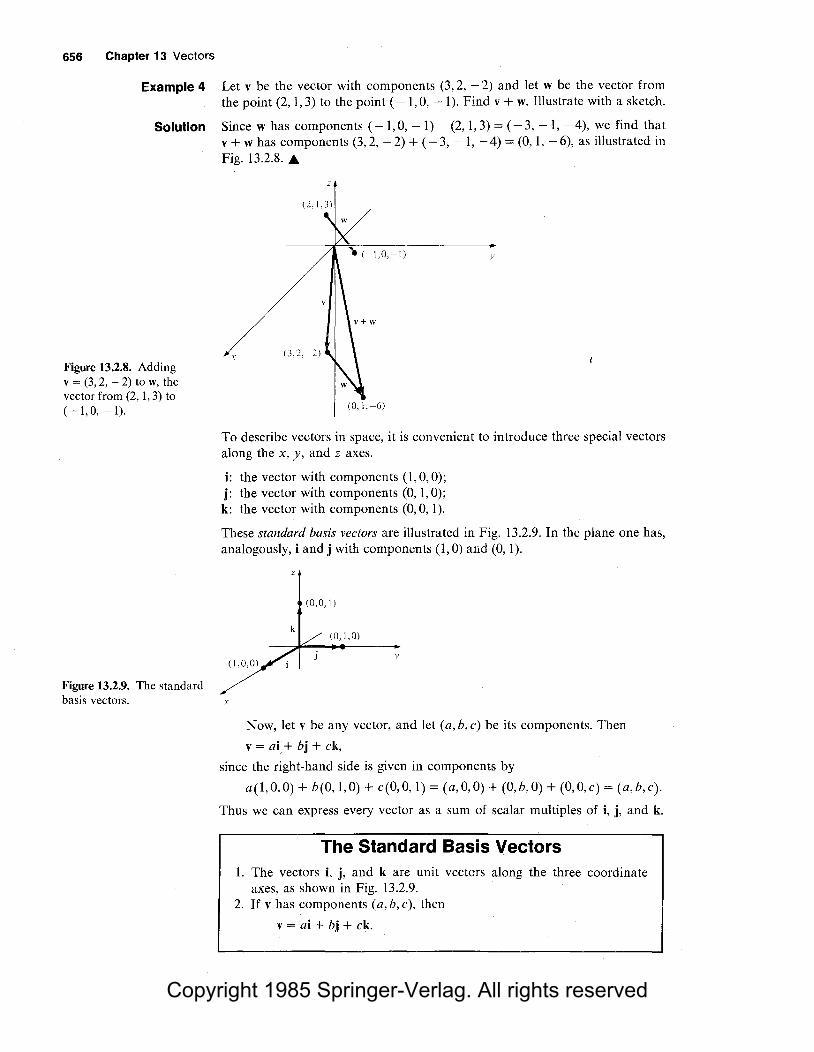
Example 4 Let v be the vector with components (3, 2, - 2) and let w be the vector from the point (2, 1, 3) to the point (-1, 0, -1). Find v + w. Illustrate with a sketch.
Solution Since w has components ( - 1, 0, - 1) - (2, 1, 3) = ( - 3, - 1, - 4), we find that v + w has components (3, 2, - 2) + ( - 3, - 1, -4) = (0, 1, - 6), as illustrated in Fig. 13.2.8 . .A.
Figure 13.2.8. Adding v = (3, 2, - 2) to w, the vector from (2, 1, 3) to (-1,0, -1).
Figure 13.2.9. The standard basis vectors.
z
y
x
I (o, 1,-6)
To describe vectors in space, it is convenient to introduce three special vectors along the x, y, and z axes.
i: the vector with components (1, 0, O); j: the vector with components (0, 1, O); k: the vector with components (0, 0, 1 ).
These standard basis vectors are illustrated in Fig. 13.2.9. In the plane one has, analogously, i and j with components (1, 0) and (0, 1).
x
z
(0,0, 1)
k (0, 1,0)
y
Now, let v be any vector, and let (a, b, c) be its components. Then
v = ai + bj + ck,
since the right-hand side is given in components by
a(l,0,0) + b(O, 1,0) + c(O,O, 1) = (a,0,0) + (O,b,O) + (0,0,c) = (a,b,c).
Thus we can express every vector as a sum of scalar multiples of i, j, and k.
The Standard Basis Vectors 1. The vectors i, j, and k are unit vectors along the three coordinate
axes, as shown in Fig. 13.2.9. 2. If v has components (a, b, c), then
v = ai + bj + ck.

Copyright 1985 Springer-Verlag. All rights reserved
13.2 Vectors in Space 657
Example 5 (a) Express the vector whose components are (e,7T, -if) in the standard basis. (b) Express the vector v joining (2, 0, 1) to ( ~, 7T, - 1) by using the standard basis.
Solution (a) v = ei + 7Tj - ff k. (b) The vector v has components ( ~, 7T, - 1) - (2, 0, 1) = (- ~,7T, -2), so v = - ~i + 7Tj - 2k .....
Example 6
Solution
Figure 13.2.10. Vector methods can be used to locate objects.
Position I after I hour
I 10 I~
I f2 I
-- ___ _J
Initial 10 position -J2 Figure 13.2.11. If an object moves northeast at IO kilometers per hour, its velocity vector has components (IO/ y'2, IO/ y'f ).
Now we turn to some physical applications of vectors.3 A simple example of a physical quantity represented by a vector is a displacement. Suppose that, on a part of the earth's surface small enough to be considered flat, we introduce coordinates so that the x axis points east, they axis points north, and the unit of length is the kilometer. If we are at a point P and wish to get to a point Q, the displacement vector u joining P to Q tells us the direction and distance we have to travel. If x and y are the components of this vector, the displacement of Q from P is "x kilometers east, y kilometers north."
Suppose that two navigators, who cannot see one another but can communicate by radio, wish to determine the relative position of their ships. Explain how they can do this if they can each determine their displacement vector to the same lighthouse.
Let P 1 and P2 be the positions of the ships and Q be the position of the lighthouse. The displacement of the lighthouse from the ith ship is the vector U; joining P; to Q. The displacement of the second ship from the first is the vector v joining P1 to P2 • We have v + u2 = u1 (Fig. 13.2.10), so v = u1 - u2 •
~~ =-= ~ . ''_I'~Q Fo~
P2 ~ L__ -- !_---
That is, the displacement from one ship to the other is the difference of the displacements from the ships to the lighthouse . .A.
We can also represent the velocity of a moving object as a vector. For the moment, we will consider only objects moving at uniform speed along straight lines-the general case is discussed in Section 14.6. Suppose, for example, that a boat is steaming across a lake at 10 kilometers per hour in the northeast direction. After 1 hour of travel, the displacement is (10/i/2, 10/i/2)~ ~ (7.07, 7.07) (see Fig. 13.2.11). The vector whose components are (10/ i/2, 10 / i/2) is called the velocity vector of the boat. In general, if an object is moving uniformly along a straight line, its velocity vector is the displacement vector from the position at any moment to the position 1 unit of time later. If a
3 Historical note: Many scientists resisted the use of vectors in favor of the more complicated theory of quaternions until around 1900. The book which popularized vector methods was Vector Analysis, by E. B. Wilson (reprinted by Dover in 1960), based on lectures of J. W. Gibbs at Yale in 1899-1900. Wilson was reluctant to take Gibbs' course since he had just completed a full-year course in quaternions at Harvard under J. M. Pierce, a champion of quaternionic methods, but was forced by a dean to add the course to his program. (For more details, see M. J. Crowe, A History of Vector Analysis, University of Notre Dame Press, 1967.)

Copyright 1985 Springer-Verlag. All rights reserved
658 Chapter 13 Vectors
Displacement due to current
displacement
Figure 13.2.12. The total displacement is the sum of the displacements due to the engine and the current.
Figure 13.2.13. The velocity w of the wind can be estimated by comparing the "wingflap" velocity v with the actual velocity v + w.
Figure 13.2.14. The magnitude and direction of electrical flow in the heart are indicated by the cardiac vector.
current appears on the lake, moving due eastward at 2 kilometers per hour, and the boat continues to point in the same direction with its engine running at the same rate, its displacement after 1 hour will have components given by (10/[i + 2, 10/[i). (See Fig. 13.2.12.) The new velocity vector, therefore, has components (10/[i + 2, 10/[i). We note that this is the sum of the original velocity vector (10 / fi, 10 / fi) of the boat and the velocity vector (2, 0) of the current.
Similarly, consider a seagull which flies in calm air with velocity vector v. If a wind comes up with velocity w and the seagull continues flying "the same way," its actual velocity will be v + w. One can "see" the direction of the vector v because it points along the "axis" of the seagull; by comparing the direction of actual motion with the direction of v, you can get an idea of the wind direction (see Fig. 13.2.13).
Another example comes from medicine. An electrocardiograph detects the flow of electricity in the heart. Both the magnitude and the direction of the net flow are of importance. This information can be summarized at every instant by means of a vector called the cardiac vector. The motion of this vector (see Fig. 13.2.14) gives physicians useful information about the heart's function.4
''"·"-'·'':I Cardiac vector at one moment
Tip of cardiac vector moving in space
Example 7 A bird is flying in a straight line with velocity vector lOi + 6j + k (in kilometers per hour). Suppose that (x, y) are coordinates on the ground and z
is the height above the ground.
(a) If the bird is at position (1, 2, 3) at a certain moment, where is it 1 minute later?
(b) How many seconds does it take the bird to climb 10 meters?
Solution (a) The displacement vector from (1, 2, 3) is fo(lOi, 6j, k) =ii+ J'oj + fok, so the new position is (1,2,3) + (i,J'ofo) = (ti,2J'o,3fo). (b) After t seconds(= t/3600 hours), the displacement vector from (l,2,3) is (t/3600)(10i + 6j + k) = (t/360)i + (t/600)j + (t/3600)k. The increase in altitude is the z component t /3600. This will equal 10 meters ( = 1/io kilometer) when t / 3600 = l / 100-that is, when t = 36 seconds. A
4 See M. J. Goldman, Principles of Clinical Electrocardiography, 8th edition, Lange, 1973, Chapters 14 and 19.

Copyright 1985 Springer-Verlag. All rights reserved
13.2 Vectors in Space 659
Example 8 Physical forces have magnitude and direction and may thus be represented by vectors. If several forces act at once on an object, the resultant force is represented by the sum of the individual force vectors. Suppose that forces i + k and j + k are acting on a body. What third force must we impose to counteract these two-that is, to make the total force equal to zero?
Solution The force v should be chosen so that (i + k) + (j + k) + v = O; that is v = - (i + k) - (j + k) = - i - j - 2k. (Here 0 is the zero vector, the vector whose components are all zero.) .&.
Exercises for Section 13.2 Plot the points in Exercises 1-4.
1. (1, 0, 0) 3. (3, - 1, 5)
2. (0, 2,4) 4. (2, -1,-!)
Complete the computations in Exercises 5-8. 5. (6, 0, 5) + (5, 0, 6) = 6. (0,0,0) + (0,0,0) =
7. (1, 3, 5) + 4(-1, -3, -5) =
8. (2,o, 1)- 8(3, -LD =
9. Sketch v, 2v, and -v, where v has components (1, - 1, -1).
10. Sketch v, 3v, and - !v, where v has components (2, - 1, 1).
11. Let v have components (0, l, 1) and w have components (1, 1, 0). Find v + w and sketch.
12. Let v have components (2, -1, 1) and w have components (1, -1, -1). Find v +wand sketch.
In Exercises 13-20, express the given vector in terms of the standard basis.
13. The vector with components ( - 1, 2, 3). 14. The vector with components (0, 2, 2). 15. The vector with components (7, 2, 3). 16. The vector with components ( - l, 2, 'TT). 17. The vector from (0, 1,2) to (1, 1, 1). 18. The vector from (3, 0, 5) to (2, 7, 6). 19. The vector from (1, 0, 0) to (2, -1, 1). 20. The vector from (1, 0, 0) to (3, - 2, 2).
21. A ship at position (1, 0) on a nautical chart (with north in the positive y direction) sights a rock at position (2, 4). What is the vector joining the ship to the rock? What angle does this vector make with due north? This is called the bearing of the rock from the ship.
22. Suppose that the ship in Exercise 21 is pointing due north and travelling at a speed of 4 knots relative to the water. There is a current flowing due east at I knot. (The units on the chart are nautical miles; 1 knot = 1 nautical mile per hour.) (a) If there were no current, what vector u
would represent the velocity of the ship relative to the sea bottom?
(b) If the ship were just drifting with the current, what vector v would represent its velocity relative to the sea bottom?
(c) What vector w represents the total velocity of the ship?
( d) Where would the ship be after 1 hour? (e) Should the captain change course? (f) What if the rock were an iceberg?
23. An airplane is located at position (3, 4, 5) at noon and travelling with velocity 400i + 500j - k kilometers per hour. The pilot spots an airport at position (23, 29, 0). (a) At what time will the plane pass directly
over the airport? (Assume that the earth is flat and that the vector k points straight up.)
(b) How high above the airport will the plane be when it passes?
24. The wind velocity v1 is 40 miles per hour from east to west while an airplane travels with air speed v2 of 100 miles per hour due north. The speed of the airplane relative to the earth is the vector sum v1 + v2 •
(a) Find v1 + V2.
(b) Draw a figure to scale. 25. A force of 50 lbs is directed 50° above horizon
tal, pointing to the right. Determine its horizontal and vertical components. Display all results in a figure.
26. Two persons pull horizontally on ropes attached to a post, the angle between the ropes being 60°. A pulls with a force of 150 lbs, while B pulls with a force of 110 lbs. (a) The resultant force is the vector sum of the
two forces in a conveniently chosen coordinate system. Draw a figure to scale which graphically represents the three forces.
(b) Using trigonometry, determine formulas for the vector components of the two forces in a conveniently chosen coordinate system. Perform the algebraic addition, and find the angle the resultant force makes with A.
27. What restrictions must be placed on x, y, and z so that the triple (x,y,z) will represent a point

Copyright 1985 Springer-Verlag. All rights reserved
660 Chapter 13 Vectors
on they axis? On the z axis? In the xy plane? In the xz plane?
28. Plot on one set of axes the eight points of the form (a, b, c ), where a, b, and c are each equal to 1 or - 1. Of what geometric figure are these the vertices?
29. Let u = 2i + 3j + k. Sketch the vectors u, 2u, and - 3u on the same set of axes.
In Exercises 30-34, consider the vectors v = 3i + 4j + 5k and w = i - j + k. Express the given vector in terms of i, j and k.
30. v + w 31. 3v 32. -2w 33. 6v + 8w 34. the vector u from the tip of w to the tip of v.
(Assume that the tails of w and v are at the same point.)
In Exercises 35-37, let v = i + j and w = -i + j. Find numbers a and b such that av + bw is the given vector.
35. i 36. j 37. 3i + 7j
38. Let u = i + j + k, v = i + j, and w = i. Given numbers r, s, and t, find a, b, and c such that au + bv + cw = ri + sj + tk.
39. A I-kilogram mass located at the origin is suspended by ropes attached to the points (1, 1, I) and (-1, -1, 1). If the force of gravity is pointing in the direction of the vector - k, what is the vector describing the force along each rope? [Hint: Use the symmetry of the problem. A I-kilogram mass weighs 9.8 newtons.]
40. Write the chemical equation CO + H 20 = H 2 + C02 as an equation in ordered triples, and illustrate it by a vector diagram in space.
41. (a) Write the chemical equation pC3H 40 3 + q02 = rC02 + sH20 as an equation in ordered triples with unknown coefficients p, q, r, ands.
(b) Find the smallest integer solution for p, q, r, ands.
(c) Illustrate the solution by a vector diagram in space.
42. Suppose that the cardiac vector is given by cos ti + sin tj + k at time t. (a) Draw the cardiac vector for t = 0, w / 4, w /2,
3w / 4, w, 5w / 4, 3w /2, 7w / 4, 2w. (b) Describe the motion of the tip of the cardiac
vector in space if the tail is fixed at the origin.
*43. Let P, =(I, 0, 0) + t(2, I, I), where t is a real number. (a) Compute the coordinates of P, for t = -1,
0, 1, and 2. (b) Sketch these four points on the same set of
axes. (c) Try to describe geometrically the set of all
the P1 •
*44. The z coordinate of the point P in Fig. 13.2.15 is 3. What are the x and y coordinates?
Figure 13.2.15. Let P = (x, y, 3). What are x andy?
•P
y
13.3 Lines and Distance
Example 1
Solution
Algebraic operations on vectors can be used to solve geometric problems.
In this section we apply the algebra of vectors to the description of lines and planes in space and to the solution of other geometric problems.
The invention of analytic geometry made it possible to solve geometric problems in the plane or space by reducing them to algebraic problems involving number pairs or triples. Vector methods also convert geometric problems to algebraic ones; moreover, the vector calculations are often simpler than those from analytic geometry, since we do not need to write down all the components.
Use vector methods to prove that the diagonals of a parallelogram bisect each other. - --Let PQRS be the parallelogram, w the vector PQ and v the vector PS (see Fig.

Copyright 1985 Springer-Verlag. All rights reserved
p
Figure 13.3.1. The diagonals of a parallelogram bisect each other.
R
Example 2
Solution
Figure 13.3.2. The point U is one-third of the way from 0 to the midpoint of the face PSQT.
13.3 Lines and Distance 661
13.3.1). Since PQRS is a parallelogram, v + w is the vector PR. The vector joining P to the midpoint M 1 of the diagonal PR is thus
f (v + w). On the other hand, the vector QS is v - w, so the vector joining Q to the midpoint M 2 of the diagonal QS is t(v - w).
To show that the diagonals bisect each other, it is enough to show that the midpoints M 1 and M 2 are the same. The vector PAI; is the sum
w + t(v- w) = w + fv- fw = w - fw + fv
=fw+fv=t(v+w)
which is the same as the vector PM1• It follows that M 1 and M 2 are the same point. .&.
Consider the cube in space with vertices at (0, 0, 0), (1, 0, 0), (1, 1, 0), (0, 1, 0), (0,0, 1), (1,0, 1), (1, 1, 1), and (0, 1, 1). Use vector methods to locate the point one-third of the way from the origin to the middle of the face whose vertices are (0, 1,0), (0, 1, 1), (1, 1, 1), and (1, 1,0). -- --Refer to Fig. 13.3.2. The vector OP is j, and vector OQ is i + j + k. The vector
z
T
x
PQis the difference i + j + k - j = i + k; the vector joining P to the midpoint R of PQ (and hence of the face PSQT) is one-half of this, that is, f (i + k); the -- : vector OR is then j + f (i + k), and the vector joining 0 to the point U
one-third of the way from 0 to R is tU +Hi+ k)] = H + 7;i + ik = ii + H + i k. It follows that the coordinates of U are (i, t, i) . .&.
Example 3 Prove that the figure obtained by joining the midpoints of successive sides of any quadrilateral is a parallelogram.
Solution Refer to Fig. 13.3.3. Let PQRS be the quadrilateral, v =JiS. w =SR, t =PQ.
Figure 13.3.3. The figure obtained by joining the midpoints of successive sides of PQRS is the parallelogram JKLM.
s
p
Q
and u =QR The vector a from the midpoint J of PS to the midpoint K of SR satisfies f v +a= v + f w; solving for a gives a= f v + f w = f (v + w). Similarly, the vector b from the midpoint M of PQ to the midpoint L of QR satisfies ft+ b = t + f u, sob= ft+ f u = t(t + u).

Copyright 1985 Springer-Verlag. All rights reserved
662 Chapter 13 Vectors
0
Figure 13.3.4. Since P, Q, and R lie on a line, the vector w - u is a multiple of v-u.
To show that JKLM is a parallelogram, it suffices to show that the vectors a and b are equal, but v + w = t + u, since both sides are equal to the vector from P to R, so a= !(v + w) = !(t + u) = b . .A.
In Section R.4 we discussed the equations of lines in the plane. These equations can be conveniently described in terms of vectors, and this description is equally applicable whether the line is the plane or in space. We will now find such equations in parametric form (see Section 10.4 for a discussion of parametric curves).
Suppose that we wish to find the equation of the line I passing through -=----the two points P and Q. Let 0 be the origin and let u and v be the vectors OP and OQ as in Fig. 13.3.4. Let R be an arbitrarzgoint on I and let w be the vector OR. Since Rison/, the vector w - u =PR is a multiple of the vector -v - u = PQ-that is, w - u = t(v - u) for some number t. This gives w = u + t(v - u) = (1 - t)u + tv.
The coordinates of the points P, Q, and R are the same as the components of the vectors u, v, and w, so we obtain the parametric equation R = (I - t)P + tQ for the line /.
Parametric Equation of a Line: Point-Point Form
The equation of the line I through the points P = (x 1, y 1, z 1) and Q = (x2 , Ji, z2) is
R = (1 - t)P + tQ.
In coordinate form, one has the three equations
x = ( 1 - t)x 1 + tx2 ,
y = (1 - t)y. + 0'2,
z = (1 - t)z 1 + tz2 ,
where R = (x, y, z) is the typical point of /, and the parameter t takes on all real values.
Example 4 Find the equation of the line through (2, l, -3) and (6, - 1, - 5).
Solution We have P = (2, 1, - 3) and Q = (6, -1, - 5), so
Figure 13.3.5. If the line through P andR has the direction of the vector d, then the vector from P to R is a multiple of d.
(x, y,z) = R = (1 - t)P + tQ = (1 - t)(2, l, -3) + t(6, -1, -5)
= (2 - 2t, 1 - t, -3 + 3t) + (6t, - t, -St)
= (2 + 4t, 1 - 2t, - 3 - 2t)
or, since corresponding entries of equal ordered triples are equal,
x=2+4t, y=l-2t, z=-3-2t . .A.
We can also ask for the equation of the line which passes through a given point Pin the direction of a given vector d. A point R lies on the line (see Fig. 13.3.5) if and only if the vector PRis a multiple of d. Thus we can describe all -points R on the line by PR= td for some number t. Ast varies, R moves on the line; when t = 0, R coincides with P. Since PR= oR - oP, we can rewrite the equation as oR = oP + td. This reasoning leads to the following conclusion.

Copyright 1985 Springer-Verlag. All rights reserved
13.3 Lines and Distance 663
Parametric Equation of a Line: Point-Direction Form
The equation of the line through the point P = (x0 , y 0 ,z0) and pointing in the direction of the vector d = ai + bj + ck is PR = td or equivalently oR. = oP + td.
In coordinate form, the equations are
x = x0 +at,
y =Yo+ bt,
z = z0 +ct,
where R = (x, y, z) is the typical point on I and the parameter t takes on all real values.
For lines in the xy plane, the z component is not present; otherwise, the results are the same.
Example 5 (a) Find the equations of the line in space through the point (3, - 1, 2) in the direction 2i - 3j + 4k.
(b) Find the equation of the line in the plane through the point (I, -6) in the direction of 5i - '1Tj.
(c) In what direction does the line x = -3t + 2, y = -2(t - 1), z = 8t + 2 point?
Solution (a) Here P = (3, -1, 2) = (x0 , y0 , z0 ) and d = 2i - 3j + 4k, so a= 2, b = - 3, and c = 4. Thus the equations are
x = 3 + 2t, y = - 1 - 3t, z = 2 + 4t.
(b) Here P = (1, - 6) and d = 5i - '1Tj, so the line is
R = (1, -6) + (5t, -?Tt) = (1+5t, -6- 7rt)
or
x = 1 + 5t, y = -6 - '1Tt.
(c) Using the preceding box, we construct the direction d = ai + bj + ck from the coefficients of t: a = - 3, b = - 2, c = 8. Thus the line points in the direction of d = - 3i - 2j + 8k. .A.
Example 6 (a) Do the lines R 1 = (t, -6t + l,2t- 8) and R 2 = (3t + l,2t,O) intersect? (b) Find the "equation" of the line segment between (1, 1, 1) and (2, 1, 2).
Solution (a) If the lines intersect, there must be numbers t 1 and t2 such that the corresponding points are equal: (t., -6t1 + l,2t1 - 8) = (3t2 + l,2t2,0); that is,
l1=3t2+l,
-6t1+1=2t2,
2t.-8=0.
From the third equation we have t1 = 4. The first equation then becomes 4 = 3t2 + 1 or t2 = 1. We must check whether these values satisfy the middle equation:
?
- 6t 1 + I .;. 2t2 , i.e.,

Copyright 1985 Springer-Verlag. All rights reserved
664 Chapter 13 Vectors
Figure 13.3.6.
I 0 PI = ~--a2'"+-b"'"2 -+-c""2 •
?
- 6 · 4 + 1 ~ 2 · 1, i.e., ?
-24 +I~ 2.
The answer is no; the lines do not intersect. (b) The line through (1, 1, 1) and (2, 1, 2) is described in parametric form by R = (1 - t)(I, 1, 1) + t(2, 1, 2) = (1 + t, 1, 1 + t), as t takes on all real values. The point R lies between (1, 1, 1) and (2, 1,2) only when 0 < t < 1, so the line segment is described by R = (1 + t, 1, 1 + t), 0 < t < 1. ..&.
Since all the line segments representing a given vector v = ai + bj + ck have the same length, we may define the length of v to be the length of any of these segments. To calculate the length of v, it is convenient to use the segment 71P, where P =(a, b, c), so that the length of v is just the distance from (0, 0, 0) to (a, b, c ). We apply the Pythagorean theorem twice to calculate this distance. (See Fig. 13.3.6.) Let Q = (a,b,O) and R = (a,0,0). Then !ORI= lal and
IRQI = lbl, so IOQI =Va2 + b2. Now I QPI =lei, so applying Pythagoras'
theorem again, this time to the right triangle OQP, we obtain I OP I = Va 2 + b2 + c2
• We denote the length of a vector v by llvll; it is sometimes called the magnitude of v as well.
z
P = (a,b,c)
y
Q=(a,b,0)
x
Length of a Vector The length llvll of a vector vis the square root of the sum of the squares of the components of v:
llai + bj + ckll =va2 + b2 + c2•
Example 7 (a) Find the length of v = 2i - 6j + 7k. (b) Find the values of c for which Iii + j + ckll = 4.
Solution (a) llvll = -/:~22_+_( --6)_2 _+_7_2 = V4 + 36 + 49 = 189 ~ 9.434.
Figure 13.3.7. The law of cosines applied to vectors.
(b) We have Iii+ j + ckll = Vl + 1 + c2 = Vl + c2. This equals 4 when 2 + c2
= 16, or c = ±ffe . ..&.
Some basic properties of length may be deduced from the law of cosines (see Section 5.1 for its proof). In terms of vectors, the law of cosines states that
llw - vll2 = llv/1 2 + llwll 2
- 211vll llwllcosB,
where Bis the angle between the vectors v and w, 0 < B < 7T. (See Fig. 13.3.7.)

Copyright 1985 Springer-Verlag. All rights reserved
u-v
In particular, since cos(} < 1, we get
jjw - vlj 2 = jjwll 2 + jjvll 2 - 2jjvjj jjwjjcos (}
? jjwjj 2 + llvll 2 - 2jjvjj jjwjj
= (llwll - llvllf
13.3 Lines and Distance 665
Taking square roots and remembering that P =!xi, we get
llw - vjj ? lllwll - llvlll·
Hence
-(llw - vii)< llwll - llvll < llw - vii·
In particular, from the right-hand inequality, we get
llwll < llw - vii+ llvll·
That is, the length of. one side of a triangle is less than or equal to the sum of the lengths of the other sides. If we write u = w - v, then w = u + v, and the inequality above takes the useful form
llu +vii < jjujj + jjvjj,
which is called the triangle inequality. The relation between length and scalar multiplication is given by
jjrvjj = lrl jjvjj
since, if v = ai + bj + ck, then
llrvjj = ~(ra)2 + (rb)2
+ (rc)2 = {r2 Ja 2 + b2 + c2 = lrlllvll·
Properties of length If u, v, and w are any vectors and r is any number:
(1) !lull > 0; (2) llull = 0 if and only if u = O; (3) llrull = lrl liujl; (4) llu +vii < jjujj + jjvjj; } . . .
(4') jjw - vii ? lllwjj - llvlll· Triangle mequahty
Example 8 (a) Verify the triangle inequality (4) for u = i + j and v = 2i + j + k.
Solution
(b) Prove that llu - vjj < llu - wjj + llw - vii for any vectors u, v, w. Illustrate with a figure in which u, v, and w are drawn with the same base point, that is, the same "tail."
(a) We have u + v = 3i + 2j + k, so llu +vii =v9 + 4 + 1 =ffe. On the other hand, !lull = fi and llvll = 16, so the triangle inequality asserts that /i4 < fi + 16. This is indeed true, since /i4 ~ 3.74, while fi + /6 ~ 1.41 + 2.45 =
3.86. (b) We find that u - v = (u - w) + (w - v), so the result follows from the triangle inequality with u replaced by u - w and v replaced by w - v. Geometrically, we are considering the shaded triangle in Fig. 13.3.8. A.
Figure 13.3.8. Illustrating The length of a vector can have interpretations other than the geometric one the inequality given above. For example, suppose that an object is moving uniformly along a llu - vii ,,;; llu - wll + llw -vii· straight line. What physical quantity is represented by the length of its velocity
vector? To answer this, let v be the velocity vector. The displacement vector from its position P at any time to its position Q, t units of time later, is tv. The

Copyright 1985 Springer-Verlag. All rights reserved
666 Chapter 13 Vectors
w
distance between P and Q is then ltlllvll, so the length llvll of the velocity vector represents the ratio of distance travelled to elapsed time-it is called the speed.
A vector o is called a unit vector if its length is equal to 1. If v is any nonzero vector, llvll =I= 0 then we can obtain a unit vector pointing in the direction of v by taking o = (I/ llvll)v. In fact,
11011 =II H vii= H llvll = 1.
We call o the normalization of v.
Example 9 ea) Normalize v = 2i + 3j -1k. eb) Find unit vectors o, v, and win the plane such that o + v = w.
Solution ea) We have llvll = -/22 + 32 + I /22 =(I /2)v'53, so the normalization of v is
o = - 1-v = _i_i + - 6-j- - 1-k. 11v11 v153 v153 v153
eb) A triangle whose sides represent o, v, and w must be equilateral as in Fig. 13.3.9. Knowing this, we may take w = i, o = 1i +elf /2)j, v = 1i - elf /2)j. Check that lloll = llvll = llwll = I and that o + v = w. A
Figure 13.3.9. The vectors u, v, and ware represented by the sides of an equilateral traingle.
Finally, we can use the formula for the length of vectors to obtain a formula for the distance between any two points in space. If Pi= exi, y 1,zi) and P2 = ex2, y 2 ,z2), then the distance between Pi and P2 is the length of the vector from P2 to Pi; that is,
IPiP2I = ll(xi - x2)i +(Yi - Yz)j + (zi - z2)kll
= J(xi - X2)2 +(Yi - Yz)2 + (zi - z2)2 ·
Distance Formula If Pi has coordinates exi,Yi,Zi) and P2 has coordinates (x2,Yz,z2), then the distance between Pi and P 2 is
J(xi - x2)2 +(Yi - Yz)2 + (zi - z2)2 ·
Example 10 ea) Find the distance between e2, 1, 0) and (3, - 2, 6). (b) Let P1 = t(l, I, I).
(i) What is the distance from P1 to (3, 0, O)? (ii) For what value of t is the distance shortest?
(iii) What is the shortest distance?
Solution (a) The distance is
~(2 - 3)2 + [I - ( - 2) J2 + (0 - 6)2 = VC -1)2 + 32 + ( - 6)2
=~I + 9 + 36 = /46 .
(b) (i) By the distance formula, the distance is

Copyright 1985 Springer-Verlag. All rights reserved
13.3 Lines and Distance 667
~(t - 3)2 + (I - 0)2 + (I - 0)2
= ,/12 - 61 + 9 + 12 + 12 = ,/312
- 61 + 9 .
(ii) The distance is shortest when 312 - 61 + 9 is least--that is, when (d/ d1)(312
- 61 + 9) = 61 - 6 = 0, or I= 1. (iii) For I = 1, the distance in (i) is /6 . .A
Exercises for Section 13.3 Use vector methods in Exercises 1-6.
I. Show that the line segment joining the midpoints of two sides of a triangle is parallel to and has half of the length of the third side.
2. Prove that the medians of the triangle intersect in a point two-thirds of the way along any median from a vertex to the midpoint of the opposite side.
3. Prove that if PQR is a triangle in space and b > 0 is a number, then there is a triangle with sides parallel to those of PQR and side lengths b times those of PQR.
4. Prove that if the corresponding sides of two triangles are parallel, then the lengths of corresponding sides have a common ratio. (Assume that the triangles are not degenerated into lines.)
5. Find the point in the plane two-thirds of the way from the origin to the midpoint of the line segment between (I, I) and (2, - 2).
6. Let P = (3, 5, 2) and Q = (2, 5, 3). Find the point R such that Q is the midpoint of the line segment PR.
Write equations for the lines in Exercises 7-10. 7. The line through (I, I, 0) and (0, 0, I). 8. The line through (2, 0, 0) and (0, I, 0). 9. The line through (0, 0, 0) and (I, I, I).
IO. The line through (-1, -1, 0) and (I, 8, -4). Write parametric equations for the lines in Exercises 11-14.
11. The line through the point (I, I, 0) in the direction of vector - i - j + k.
12. The line through (0, I, 0) in the direction j. 13. The line in the plane through ( - 1, - 2) and in
direction 3i - 2j. 14. The line in the plane through (2, -1) and in
direction - i - j.
15. At what point does the line through (0, I, 2) with direction i + j + k cross the xy plane?
16. Where does the line through (3, 4, 5) and (6, 7, 8) meet the yz plane?
17. Do the lines given by R 1 =(t,3t-l,4t) and R 2 = (3t, 5, I - t) intersect?
18. Find the unique value of c for which the lines R 1 = (t, -6t + c,2t - 8) and R2 = (3t + 1,2t,O) intersect.
Compute the length of the vectors in Exercises 19-24.
19. i + j + k 20. 2i + j 21. i + k 22. 3i + 4j 23. 2i + 2k 24. i - j - 3k
25. For what a is llai - 3j + kll = 16? 26. For what b is Iii - bj + 2kll = 3? 27. Verify the triangle inequality for the vectors in
Exercises I 9 and 21. 28. Verify the triangle inequality for the vectors in
Exercises 20 and 22. 29. Find unit vectors u, v, and w in the plane such
that u + 2v + w = 0. 30. Find unit vectors u, v, w, and z in the plane such
that u + v + w + z = 0. 3 I. Show that (0, 0, I) (0, I, 0), and (I, 0, 0) are the
vertices of an equilateral triangle. How long is each side?
32. Find an equilateral triangle in space which shares just one side with the one in Exercise 3 I.
33. Normalize the vectors in Exercises 19 and 21. 34. Normalize the vectors in Exercises 20 and 22.
Find. the distance between the pairs of points in Exercises 35-38.
35. (I, 1,3) and (2,2,2) 37. (I, I, 2) and (I, 2, 3)
39. Let P, = t(3, 2, I).
36. (2, 0, 0) and (2, I, 2) 38. (I, 2, 3) and (3, 2, I)
(i) What is the distance from P, to (2, 0, O)? (ii) For what value oft is the distance shortest?
(iii) What is that shortest distance? 40. Draw a figure, similar to Fig. 13.3.6, to illustrate
the distance formula on p. 666. 41. A boat whose top speed in still water is 12 knots
points north and steams at full power. If there is an eastward current of 5 knots, what is the spee<l of the boat?
42. A ship starting at (0, 0) proceeds at a speed of IO knots directly toward a buoy located at (3, 4). (The chart is measured in nautical miles; a knot equals I nautical mile per hour.) (a) What is the ship's point of closest approach
to a rock located at (2, 2)? (b) After how long does it reach this point? (c) How far is this point from the rock?
*43. Derive the point-point form of the equation of a line obtained in Section R.4 from the parametric

Copyright 1985 Springer-Verlag. All rights reserved
668 Chapter 13 Vectors
form obtained in this section. Comment on the case in which x 1 = x 2 .
V= q1 + q2 4m'ollr - r1 II 4'1TEollr - r2ll
*44. Derive the point-direction form for the parameteric equation of a line from the point-point form. [Hint: If a line through Pis to have direction d, what other point must lie on the line?]
*45. When does equality hold in the triangle inequality? (You might try using the law of cosines as was done in the text.) Test your conclusion on the vectors in Exercises 21 and 23.
*46. The potential V produced at (x, y,z) by charges q1 and q2 of opposite sign placed at distances x 1
and x 2 from the origin along the x axis is given by
13.4 The Dot Product
In this formula, r is the vector from the origin to the point (x, y, z). The vectors r 1 and r2 are vectors from the origin to the respective charges q1 and q2 •
(a) Express the formula for V entirely in terms of the scalar quantities x,y,z,x 1,x2 ,q1'
q2,Eo. (b) Show that the locus of points (x,y,z) for
which V = 0 is a plane or a sphere whose radius is Jq 1q2(x 1 - x 2)/(qT - q~)I and whose center is on the x axis or is a plane.
The dot product of two unit vectors is the cosine of the angle between them.
To introduce the dot product, we will calculate the angle B between two vectors in terms of the components of the vectors.
If v1 and v2 are two vectors, we have seen (Fig. 13.3.7) that
llv2 - V1ll2 = llvill
2 + llv2Jl2
- 2Jlv1ll llv2llcosB,
where B is the angle between v1 and v2; 0 < B < 7T. Therefore,
2JJv1ll llv2llcosB = llv111 2 + llv2Jl 2 - llv2 - V1ll 2. (1)
If v1 = a 1i + bd + c1k and v2 = a2i + b2 j + c2k, then the right-hand side of equation (1) is
(a?+ bi+ cf)+ (ai +bi+ ci)-[ (a 1 - a2)2 + (b 1 - b2)
2 + (c 1 - c2)2
]
= 2(a1a2 + b1b2 + c1c2).
Thus we have proved that
Jlv1ll llv2llcos0 = a1a2 + b1b2 + c1c2 . (2)
This very convenient formula enables us to compute cosB and hence B; thus the quantity on the right-hand side deserves a special name. If v1 = a1i + bd + c1k and v2 = a2i + b2j + c2k are two vectors, the number a1a2 + b1b2 + c1c2 is called their dot product and is denoted by v1 • v2. The dot product in the plane is defined analogously; just think of c1 and c2 as being zero.
Notice that the dot product of two vectors is a number, not a vector. It is sometimes called the scalar product (do not confuse this with scalar multiplication) or the inner product.
Example 1 (a) If v1 = 3i + j - 2k and v2 = i - j + k, calculate v1 · v2. (b) Calculate (2i + j - k) · (3k - 2j).
Solution (a) v1 • v2 = 3 · 1 + 1 · (-1) + (-2) · 1 = 3 - 1 - 2 = 0. (b) (2i + j - k) · (3k - 2j) = (2i + j - k) · (Oi - 2j + 3k) = 2 · 0 - 1 · 2 - 1 · 3 = -5 .....
Combining formula (2) with the definition of the dot product gives
!Iv 1 II llv2llcos B = V1 · V2, (3)
where Bis the angle between v1 and v2.

Copyright 1985 Springer-Verlag. All rights reserved
13.4 The Dot Product 669
We may solve (3) for cosO to obtain the formula
cosO= V1'V2 llv1ll llv2ll
i.e., 0 = cos- 1( 11 ;1111 ' 1 ~:211 )if v1=I=0 and v2 =I= 0.
Example 2 (a) Find the angle between the vectors i + j + k and i + j - k. (b) Find the angle between 3i + j - 2k and i - j + k.
Solution (a) Let v 1 = i + j + k and v2 = i + j - k. Then llv ill = Y3, llv2ll = Y3, and v1·v2 =l·l+l·l-l·l=l. Hence cosO=t, so 0=cos- 1(t):::::;l.23 radians (70°32'). (b) From Example l(a), (3i + j - 2k) · (i - j + k) = 0, so cosO = 0 and hence 0 = 'TT/2 ...
From (3) we get
lv1 · v2I = llv1ll llv2ll lcosOI.
However, lcosOI < 1, so we have
lv1 · v2I < llvill llv2ll·
This is a useful inequality called the Schwarz inequality (and sometimes the Cauchy-Schwarz-Buniakowski inequality).
From either (2) or (3), we notice that if v = ai + bj + ck, then
v · v = a2 + b2 + c2 = llvll 2-
Since two nonzero vectors are perpendicular when 0 = 'TT /2-that is, when cos 0 = 0-we have an algebraic test for perpendicularity: the nonzero vectors v1 and v2 are perpendicular when v1 · v2 = 0. (We adopt the convention that the zero vector is perpendicular to every vector.) The synonyms "orthogonal" or "normal" are also used for "perpendicular."
The Dot Product Algebraic definition:
(a1i + bJi + c1k) • (a2i + b2j + c2k) = a1a2 .+ b1b2 + c1c2 .
Geometric interpretation:
V1 · V2 = llv 1 II llv2llcos 0,
where 0 is the angle between v1 and v2, 0 < 0 < 77. In particular,
llvll2 = v. v.
Properties:
1. u · u > 0 for any vector u. 2. u · u = 0 only if u = 0. 3. u. v = v. u. 4. (u + v) · w = u · w + v • w. 5. (au)· v = a(u · v). 6. In· vi < llnll llvll (Schwarz inequality). 7. u and v are perpendicular when u · v = 0.

Copyright 1985 Springer-Verlag. All rights reserved
670 Chapter 13 Vectors
Example 3
S-ol,utlon
Figure 13.4.1. There are two unit vectors orthogonal
Find a unit vector in the plane which is orthogonal to v = i - 3j.
If w = ai + bj is perpendicular to i - 3j, we must have 0 = v • w = a - 3b; that is, a= 3b. If w is to be a unit vector, we must also have 1 = a2 + b2 = (3b)2 + b2 = 10b2
, so b = ± 1 /{IO and a = ± 3 /{IO. Thus there are two possible solutions:(± 1/{10)(3i + j). (See Fig. 13.4.1.) A
~ (3i + j) v 10
to i - 3j. i - 3j
Example 4 Let u and v be vectors in the plane; assume that u is nonzero.
(a) Show that w = v - (v • u/u • u)u is orthogonal to u. (b) Sketch the vectors u, v, w, and v - w. The vector v - w = (v · u/u · u)u is
called the orthogonal projection of v on u. Why? (c) Find the orthogonal projection of i + j on i - 2j.
Solution (a) We compute
Figure 13.4.2. The vector v - w = (v • u/u • u)u is the orthogonal projection of v on u.
Figure 13.4.3. The orthogonal projection of v on u equals - ~ u.
u • w = u • (v - v • 0 u). u·u
By the algebraic properties of the dot product, this is equal to
u • v - v • u u • u = u • v - v • u = 0, u·u
so u • w = 0 and w is orthogonal to u. (b) We note that v - w = (v • u/u • u)u is a multiple of u. Thus the configuration of vectors must be as in Fig. 13.4.2. The vector v - w is called the orthogonal projection of v on u because it is obtained by dropping a perpendicular from the "tip" of v to the line determined by u. (The base points of u and v must be the same for this construction.) ( c) With u = i - 2j and v = i + j, the orthogonal projection of v on u is
u • v I - 2 (" 2.) 1 (" 2") --u=-- 1- J =-- 1- J· u·u 1+4 5
(See Fig. 13.4.3.) A
We can use the dot product to find the distance from a point Q = ( x 1, y 1, z 1)
to the line l which passes through a point P = (x0 , y 0 , z0) and has the direction d = ai + bj + ck. Indeed, in Fig. 13.4.4 the distance from Q to the line is the
projection of v on u
v
Figure 13.4.4. llWil is the distance from Q to I.

Copyright 1985 Springer-Verlag. All rights reserved
0
13.4 The Dot Product 671
distance between Q and R, where R is chosen on I in such a way that PR and QR are orthogonal. Then PRis the orthogonal projection of PQon the line/. Thus, by Example 4,
PR= PQ· d d = a(x1 - Xo) + b(y1 - Yo)+ c(z1 - zo) d. d . d a2 + b2 + c2
By Pythagoras' theorem, llRQil = v'llPQ11 2 - llPR'il2 which gives
as the distance from Q to the line /.
Example 5 Find the distance from (1, 1, 2) to the line through (2, 0, 0) in the direction (l/Vl)i - (l/Vl)j.
Solution In formula (4), we set (x 1,y1,z1)=(1,1,2), (x0,y0 ,z0)=(2,0,0) and obtain a, b, c from ai + b j + ck = (I/ Vi )i - ( 1 /Vi )j to be a = 1 /Vi, b = - 1 Vi, c = 0. Thus,
<fat( Q,/) +-2)' + I' + 2' _ [ t (I i : i t Ir r = (6 - 2) 1
/2 = 2 .....
The dot product makes it simple to determine the equation of a plane. Suppose that a plane f!71 passes through a point P0 =(x0 ,y0 ,z0) and is perpendicular to a vector n = Ai + Bj + Ck. (See Fig. 13.4.5.)
Figure 13.4.5. The plane fl! is perpendicular to the vector n.
Let P = (x, y,z) be a point on 9. Then n must be perpendicular to the vector v from P0 to P; that is, n · v = 0, or
(Ai+ Bj +Ck)· [ (x - x0)i + (y - y 0)j + (z - z0)k J = 0.
Hence
A (x - x0) + B(y - y 0) + C(z - z0) = 0.
We call n the normal vector of the plane. If we let D = -(Ax0 + By0 + Cz0),
the equation of the plane becomes
Ax + By + Cz + D = 0.
Example 6 Find the equation of the plane through (I, I, I) with normal vector 2i + j - 2k.
Solution Here Ai+ Bj +Ck= 2i + j - 2k, and (x0 , y 0 ,z0) =(I, I, I), so we get
A(x - I)+ B(y - I)+ C(z - I)= 0.
Hence
2(x- l)+(y- I)-2(z- l)=O,
2x + y-2z =I . ..&.

Copyright 1985 Springer-Verlag. All rights reserved
672 Chapter 13 Vectors
Example 7 Find a unit normal vector to the plane 3x + y - z = 10. Sketch the plane.
Solution A normal vector is obtained by making a vector out of the coefficients of x, y, and z; that is, (3, 1, - 1). Normalizing, we get
Figure 13.4.6. The plane 3x + y - z = 10.
(3, 1, -1)/J9 + 1+1 = (3/v'Tf, 1/v'Tf, -1/v'Tf); i.e. - 1-(3i + j - k). v1T
We may sketch the plane by noting where it meets the coordinate axes. For example, setting y = z = 0, we see that ( 3f, 0, 0) lies on the plane (see Fig. 13.4.6) ....
10 (3'0,0)
x
z
(0,10,0) /
y
Equation of a Plane in Space The equation of the plane through (x0 , y 0 , z0) with normal vector n =Ai+ Bj + Ck is
A ( x - x 0 ) + B (y - y 0 ) + C( z - z0) = 0 (5)
or
Ax + By + Cz + D = 0. (6)
Example 8 (a) Find the equation of the plane passing through the point (3, -1, -1) and perpendicular to the vector i - 2j + k. (b) Find the equation of the plane containing the points (1, 1, 1), (2, 0, 0), and (1, 1, 0).
Solution (a) We use the first displayed equation (5) in the preceding box, choosing the point (x0 , y 0 , z0) = (3, -1, -1) and components of the normal vector to be A = 1, B = - 2, C = 1 to give
l(x - 3)-2(y + 1) + l(z + 1) = 0
which simplifies to x - 2y + z = 4. (b) The general equation of a plane has the form (6) Ax+ By+ Cz + D = 0. Since the points (I, 1, 1), (2, 0, 0), and (1, I, 0) lie on the plane, the coefficients A, B, C, D satisfy the three equations:
A+B+C+D = 0, 2A +D =0, A+B +D = 0.

Copyright 1985 Springer-Verlag. All rights reserved
13.4 The Dot Product 673
Proceeding by elimination, we reduce this system to the form
2A + D = 0 (second equation),
2B + D = 0
C=O
(twice the third equation minus the second),
(first equation minus the third).
Since the numbers A, B, C, and D are determined only up to a common factor, we can fix the value of one of them and then the others will be determined uniquely. If we let D = - 2, then A = I, B = 1, C = 0. Thus x + y - 2 = 0 is an equation of the plane that contains the given points. (You may go back and verify that the given points actually satisfy this equation.) .&.
Example 9 Where does the line through the origin in the direction of i + j + 2k meet the plane x + y + 2z = 5? Use your answer to find the distance from the origin to this plane. Sketch.
Solution The line has parametric equations x = t,y = t, z = 2t. It meets the plane when x + y + 2z = t + t + 4t = 5; that is, when t = i. The point of intersection is P, = (i,i,i).
Figure 13.4.7. The vector from 0 to the closest point P 1 on a plane is perpendicular to the plane.
Figure 13.4.8. The geometry for determining the distance from a point to a plane.
Since a normal to the plane is n = i + j + 2k, which is the same as the direction vector of this line, we see that the line is perpendicular to the plane at P 1• If Pis also in the plane, consideration of the right triangle OP1P shows that OP1 must be shorter than OP (see Fig. 13.4.7). Thus the distance from the origin to the plane is the length of OP1:
25 + 25 + 25 = b650 = 5,/666 .... 36 36 9
y
(5,0,0)
x
Let A (x - x 0) + B(y - y 0) + C(z - z0) = 0 be the equation of a plane 9 through the point P = (x0 , y 0 , z 0) in space. Let us use the basic ideas of the preceding example to determine the distance from a point Q = (x 1, y 1,z1) to the plane (see Figure 13.4.8). Consider the vector

Copyright 1985 Springer-Verlag. All rights reserved
674 Chapter 13 Vectors
Ai+ Bj +Ck n= ---;::::======= )A2+B2+c2,
which is a unit vector normal to the plane. Next drop a perpendicular from Q to the plane and construct the triangle PQR shown in Figure 13.4.8. The distance d = RQ is the length of the projection of v = PQ (the vector from P to Q) onto n; thus
distance = Iv · nl = I [ ( x 1 - x0)i + (y 1 - y 0)j + ( z 1 - z0)k J • nl IA (x1 - xo) + B(y1 - Yo)+ C(z1 - zo)I
)A2+B2+c2
If the plane is given in the form Ax + By + Cz + D = 0, choose a point (x0 , y 0 , z0) on it and note that D = - (Ax0 + By0 + Cz0). Substituting in the previous formula gives
. ai 1Ax1 +By1+Cz1+DI dist( Q, er) = (7)
VA2+B2+C2
for the distance from Q to 9.
Example 10 Find the distance from Q = (2,0, -1) to the plane 9: 3x - 2y + 8z + 1=0.
Solution We substitute into (7) the values x 1 = 2,y1 = 0, z1 = -1 (from the point) and A= 3, B = -2, C = 8, D = 1 (from the plane) to give
. 13 · 2 + ( - 2) · o + 8( - 1) + 11 1- 11 1 dist(Q,9) = = -- = - . A
Exercises for Section 13.4 Compute the dot products in Exercises 1-4.
I. (i + j + k)- (i + j + 2k) 3. i. j
2. (i + j + k) • (i + k) 4. (3i + 4j) . (3j + 4k)
5. Find the angle between the pair of vectors in Exercise l.
6. Find the angle between the pair of vectors in Exercise 2.
7. Find the angle between the pair of vectors in Exercise 3.
8. Find the angle between the pair of vectors in Exercise 4.
9. Find a unit vector in the xy plane which is orthogonal to 2i - j.
10. Find a unit vector in the xy plane which is orthogonal to 3j - 5i.
11. Use the formula (i + j + k) · i = l to find the angle between the diagonal of a cube and one of its edges. Sketch.
12. (a) Show that if llull = llvll, and u and v are not parallel, then u + v and u - v are perpendicular. (b) Use the result of part (a) to prove that
)32 + (-2)2 + 82 {Fi {Fi
any triangle inscribed in a circle, with one side of the triangle as a diameter, is a right triangle.
13. Show that the length of the orthogonal projection of v on u is equal to llvll lcos (JI, where (J is the angle between v and u.
14. Use vector methods to prove that a triangle is isosceles if and only if its base angles are equal.
15. Find the distance from (2, 8, -1) to the line through (l, l, l) in the direction of the vector (l / vJ)i + (l I vJ)j + (l / vJ)k.
16. Find the distance from (1, l, -1) to the line through (2, - I, 2) in the direction of k.
17. Find the distance from (1, l, 2) to the line x = 3 t + 2, y = - t - I, z = t + l.
18. Find the distance from (l, 1, 0) to the line through (l, 0, -1) and (2, 3, 1).
Give the equation for each of the planes in Exercises 19-24.
19. The plane through the origin orthogonal to the vector i + j + k.
20. The plane through (1, 0, 0) orthogonal to the vector i + j + k.

Copyright 1985 Springer-Verlag. All rights reserved
21. The plane through the origin orthogonal to i. 22. The plane containing (a,b,c) with normal vector
ai + bj +ck. 23. The plane containing the points (0, 0, 1), (1, 1, 1)
and (0, 1, 0). 24. The plane containing the points (1, 0, 0), (0, 2, 0),
and (0, 0, 3). Find a unit vector orthogonal to each of the planes in Exercises 25-28.
25. The plane given by 2x + 3y + z = 0. 26. The plane given by 8x - y - 2z + 10 = 0. 27. The plane through the origin containing the
points (1, 1, 1) and (1, 1, -1). 28. The plane containing the line (1 + t, 1 - t, t) and
the point (1, 1, 1). Find the equation of the objects in Exercises 29-32.
29. The plane containing (0, 1, 0), (1, 0, 0), (0, 0, 1). 30. The line through (1, 2, l) and ( - 1, 1, 0). 31. The line through (1, 1, 1) and orthogonal to the
plane in Exercise 29. 32. The line through (0, 0, 0) which passes through
and is orthogonal to the line in Exercise 30.
33. Where does the line through the origin in the direction of 2i - j + 3k meet the plane 2x - y + 3z = 7? Find the distance from the origin to this plane.
34. Where does the line through P = (1, 1, 1) in the direction of 2i - j + 3k meet the plane 2x - y + 3z = 7? Find the distance from P to this plane.
35. The planes 3x + 4y + 5z = 6 and x - y + z = 4 meet in a line. Find the parametric equations of this line.
36. Find the parametric equations of the line where the plane x + y = z meets the plane y + z = x.
37. Find the distance from the point (1, 1, 1) to the plane x - y - z + 10 = 0.
38. Find the distance from the point (2, - 1, 2) to the plane 2x - y + z = 5.
39. Find the distance from the origin to the plane through (1, 2, 3), ( -1, 2, 3), and (0, 0, 1).
40. Find the distance from the point (4, 2, 0) to the plane through (0, 0, 0), (1, 1, 1), and (1, 1, 2).
41. Show that the locus of points in the plane equidistant from two given points is a line, and give an equation for that line in terms of the coordinates of the two points.
42. Use vector methods to show that if three parallel lines in the plane cut off equal segments on one transversal, then they do so on any transversal.
43. Compute the following: (a) (3i + 2j - k) · (j - k). (b) [(3i-j-k)-(i+j)]·j. (c) The distance between (1, 0, 2) and (3, 2, 4). (d) The length of (i - j - k) + (2j - k + i).
13.4 The Dot Product 675
44. Find the following: (a) A unit normal to the plane x - 2y + z = 0. (b) A vector orthogonal to the vectors i - j + k
and i + j + k. (c) The angle between 2i + j + k and k - i. (d) A vector in space making an angle of 45°
with i and 60° with j. 45. Let P 1 and P2 be points in the plane. Give an
equation of the form ax + by = c for the perpendicular bisector of the line segment between P 1
and P2 •
46. Given nonzero vectors a and b, show that the vector v = llallb + llhlla bisects the angle between a and b.
Exercises 47-50 form a unit. 47. Suppose that e1 and e2 are perpendicular unit
vectors in the plane, and let v be an arbitrary vector. Show that v = (v • e 1)e1 + (v · e2)e2 • The numbers v • e1 and v • e2 are called the components of v in the directions of e1 and e2 . This expression of v as a sum of vectors pointing in the directions of e1 and e2 is called the orthogonal decomposition of v relative to e1 and e2 .
48. Consider the vectors e1 = (1 / y'2 )(i + j) and e2
= (l / y'2 )(i - j) in the plane. Check that e1 and e2 are unit vectors perpendicular to each other and express each of the following vectors in the form v = a 1e1 + a2e2 (that is, as a linear combination of e 1 and e2):
(a) v = i,
(c) v = 2i + j, (b) v=j, (d) v = -2i - j.
49. Suppose that a force F (for example, gravity) is acting vertically downward on an object sitting on a plane which is inclined at an angle of 45° to the horizontal. Express this force as a sum of a force acting parallel to the plane and one acting perpendicular to it.
50. Suppose that an object moving in direction i + j is acted on by a force given by the vector 2i + j. Express this force as a sum of a force in the direction of motion and a force perpendicular to the direction of motion.
51. A force of 6 newtons makes an angle of 'TT/ 4 radians with they axis, pointing to the right. The force acts against the movement of an object along the straight line connecting (1, 2) to (5, 4). (a) Find a formula for the force vector F. (b) Find the angle (} between the displacement
direction D = (5 - l)i + (4 - 2)j and the force direction F.
(c) The work done is F · D, or equivalently, llFll 11Dllcos8. Compute the work from both formulas and compare.
52. A fluid flows across a plane surface with uniform vector velocity v. Let n be a unit normal to the plane surface. Show that v · n is the volume of fluid that passes through a unit area of the plane in unit time.

Copyright 1985 Springer-Verlag. All rights reserved
676 Chapter 13 Vectors
53. Establish the following properties of the dot product: (a) u · u > 0 for any vector u. (b) If u · u = 0, then u = 0. (c) u• v = v •u for any vector u and v. (d) (au+ bv) · w = a(u · w) + b(v · w) for any
numbers a and b and. any vectors u, v, w. 54. Let:
L 1 =the line (2, 1, 1) + t(l, 1, l); Lz =the line (1 + 7t, 7t - 2, 2 + 7t); L 3 = the line (1, 0, 8) + t(l, 1, 9); L4 =the line through the points (-1, O, 1) and
(1,2, 19). (a) D~termine whether each of the following
palfs of lines is parallel or intersects. If the lines intersect, find the point of intersection.
(i) L 1 and L 2
(ii) L2 and L3
(iii) L 1 and L 3
(iv) L 2 and L 4
(v) L 1 and L4
(vi) L3 and L4
(b) For each pair of lines in part (a) which lie in a plane (that is, are not skew), find an equation for that plane.
(c) For each of the lines L 1 to L 4 , find the point of the closest approach to the origin and an equation for the plane perpendicular to that line through that point.
Lll 55. A construction worker is checking the architect's plans for some sheet metal construction. One diagram contains a triangle with sides 12.5, 16.7, 20.9, but no angles have been included. The worker gets out a calculator to check that (12.5? + (16.7)2 ~ (20.9)2
, then marks the angle opposite the long side as 90°. (a) Explain from the law of cosines the reason
why the worker's actions are essentially correct.
(b) The angle is not exactly 90°, from the data given. What percentage error is present?
*56. Let P1 and P2 be points in the plane with polar coordinates (r 1, 81) and (r2 , 82), respectively, and let u1 be the vector from 0 to P 1 and u2 the vector from 0 to P2 • Show that u1 • u2 = r1r2cos(81 - 82). [Hint: Use a trigonometric identity.]
*.57. Suppose that R = P0 + t(a, b, c) is the line through P0 in the direction d = ai + bj + ck. Let u=d/lldll =(µ,A.,v). Let:
a= angle from i to d; /3= angle from j to d; y = angle from k to d.
These are called the direction angles of the line. The numbers cos a, cos {3, and cosy are called its direction cosines (see Fig. 13.4.9).
k
Figure 13.4.9. The direction angles of the line l are a, {3, and y.
d
(a) Show that P0 +s(µ,A.,v) gives the same line. (What values of s and t correspond to the same points on the line?)
(b) Show that cosa=i·u=µ; cosf3=j·u =A.; cosy= k. u = v.
(c) Show that cos2a + cos2f3 + cos2y = 1. ( d) Determine the direction angles and cosines
of each of the lines in Exercise 54. (e) Which lines through the origin have direc
tion angles a = f3 = y? *58. Imagine that you look to the side as you walk in
the rain. Now you stop walking. (a) How does the (apparent) direction of the
falling rain change? (The rain may be falling at an angle because of wind.)
(b) Explain the observation in (a) in terms of vectors.
(c) Suppose that there is no wind and that you know your walking speed. How could you measure the speed at which the rain is falling?
(d) Do part (c) if the rain is falling at an angle.

Copyright 1985 Springer-Verlag. All rights reserved
13.5 The Cross Product 677
13.5 The Cross Product
Figure 13.5.1. The point P has velocity vector v.
Figure 13.5.3. Calculating the area of ORQP.
Example 1
Solution
The cross product of two vectors in space is a new vector that is perpendicular to the first two.
What is the velocity of a point on a rotating object? Let v1 be a vector which points in the direction of the axis of rotation and whose length equals the rotation rate (in radians per unit time). Let v2 be a vector from a point 0 on the axis of rotation to a point P on the object (see Fig. 13.5. l ). A little thought shows that the velocity v of the point P has the following properties:
l. llvll = llv1ll llv2 llsin0, where Bis the angle between v1 and v2 •
2. If B =I= 0 (so that v =I= 0), vis perpendicular to both v1 and v2 , and the triple (v1, v2 , v) of vectors obeys the right-hand rule (see Fig. 13.5.2).
Figure 13.5.2. Right-hand rule: Place the palm of your hand so that your fingers curl from v 1 in the direction of v2 through the angle B. Then your thumb points in the direction of v.
v
Note that condition l says the magnitude of the velocity of P is proportional to the product of the magnitude of the rotation rate and the distance of P from the axis of rotation; furthermore, for fixed llv2 11, the velocity is greatest when v2 is perpendicular to the axis.
Conditions land 2 determine v uniquely in terms of v1 and v2 ; vis called the cross product (or vector product) of v1 and v2 and is denoted by v1 X v2 .
We will now determine some properties of the cross product operation. Our ultimate goal is to find a formula for the components of v1 X v2 in terms of the components of v1 and v2 • Let us first show that llv1 X v2 ll is equal to the area of the parallelogram spanned by v1 and v2 • Drop the perpendicular PS as shown in Fig. 13.5.3. Then A= !ORI !PSI= !ORI IOPlsinB = llvill llv2 llsin0 = Jlv 1 x v2 ll by condition 1, proving our claim.
Find all the cross products between the standard basis vectors i, j, and k.
We observe first that i Xi= j X j = k X k = 0, because the angle between any vector and itself is zero, and sin 0 = 0. Next we observe that i X j must be a multiple of k, since it is perpendicular to i and j. On the other hand, Iii X ill = II ill Iii II sin 90° = 1, soi X j must be k or - k. The right-hand rule then

Copyright 1985 Springer-Verlag. All rights reserved
678 Chapter 13 Vectors
Figure 13.5.4. The right-hand rule requires that i X j equal k, not - k.
Figure 13.5.5. As we go around the circle, the cross product of any two consecutive vectors equals the third vector. Going backwards produces the negative of the preceding vector.
shows that i X j = k (see Fig; 13.5.4). Next, j x i must be k or - k; this time the right-hand rule gives - k as the answer. Similarly, j x k = i, k X i = j, k x j = -- i, and i x k = - j . .A
A good way to remember these products is to write i, j, and k in a circle as in Fig. 13.5.5.
We will now obtain a general formula for the cross product
(a1 i + bd + c1k) x (a2 i + b2 j + c2 k). If we assumed that the usual rules of algebra apply to the cross product, we could use the result of Example l to make the following calculation:
(a 1i + bd + c1k) X (a2i + b2j + c2k)
= a 1i X (a2i + b2j + c2k) + bd X (a2i + b2j + c2k) + c1k X (a2i + b2j + c2~ = a 1b2k + a 1c2(-j) + b 1a2(-k) + b 1c2i + c1a2j + c 1b2(-i).
Collecting terms, we have
(a 1i + bd + c1k) X (a2i + b2j + c2k)
= (b 1c2 - c1b2)i + (c 1a2 - a 1c2)j + (a 1b2 - b 1a2)k. (1)
Although to derive (1) we made the unjustified assumption that some laws of algebra hold for the cross product, it turns out that the result is correct. To see this, we shall show that u = (b 1c2 - c1b2)i + (c 1a2 - a 1c2)j + (a 1b2 - b 1a2)k is indeed the cross product of v1 = a 1i + bd + c1k and v2 = a2i + b2j + c2k. We accomplish this by verifying that u satisfies conditions I and 2 in the definition of the cross product.
First, we consider the squared length of u:
(b 1c2 - c1b2)2+ (c 1a2 - a 1c2)2+ (a 1b2 - b1a2)2
= bfd - 2b 1c 1b2c2 + cfbi + cfai - 2a 1c 1a 2c2 + afd + afbi - 2a 1b 1a2b2 + bfai
Now we compute the square of llvifl llv2llsinO:
llv 1 ll 2llv2ll 2sin20 = llv 1 ll2llv2ll\ l - cos20)
= llv1ll2
llv2ll2
- (llv1ll llv2llcos0)2
= Jlvifl 2llv211 2 - (v 1 • v2)2
= (af +bf+ cf)(ai +hi+ d)- (a 1a2 + b1b2 + c 1c2)2
which, when it is multiplied out and terms are collected, is the same as llnll2, so llnll = llvifl llv2llsinO.
Next we check that u is perpendicular to v1 and v2. We have
u · v 1 = ( b1c2 - c1b2)a1 + ( c1a2 - a 1c2)h:1 + ( a 1b2 - b1a2)c1
= b1c2a1 - c1b2a 1 + c 1a2b 1 - a1c2b1 + a 1b2c1 - b 1a 2c 1
=0,

Copyright 1985 Springer-Verlag. All rights reserved
13.5 The Cross Product 679
since the terms cancel in pairs. Similarly, u · v2 = 0, sou is perpendicular to v1 and v2.
To check the right-hand rule would require a precise mathematical definition of that rule, which we will not attempt to give. Instead, we will merely remark that the rule is satisfied for all products of standard basis vectors; see Example I.
We have now shown that the vector u on the right-hand side of (1) satisfies the conditions in the definition of v1 X v2, so it must be v1 X v2. The algebraic rules in the following display may then be verified as a consequence of formula (I) (see Example 7).
The Cross Product Geometric definition: v1 X v2 is the vector such that:
l. llv1 X v2ll = llv1ll llv2llsin0, the area of the parallelogram spanned by v1 and v2 (0 is the angle between v1 and v2; 0 < 0 <'IT).
2. Vix v2 is perpendicular to v1 and v2, and the triple (vi, v2, vi X v2) obeys the right-hand rule.
Component formula:
( aii + b1j + cik) X ( a2i + b2j + c2k)
= (bic2 - Cib2)i + (cia2 - a 1c2)j + (a 1b2 - b1a2)k
Algebraic rules:
I. v1 X v2 = 0 if and only if Vi and v2 are parallel or Vi or v2 is zero. 2. Vi Xv2= -v2XVi. 3. Vi X (V2 + V3) =Vi X V2 +Vi X V3. 4. (Vi + V2) X V3 = V1 X V3 + V2 X v3. 5. (avi) X v2 = a(vi X v2).
Multiplication table (see Fig. 13.5.5):
Second Factor x j k
First i - 0 k -j
Factor j -k 0 k j -i 0
Example 2 (a) Compute (3i + 2j - k) x (j - k). (b) Find ix (ix j) and (ix i) x j. Are they equal?
Solution (a) We use the products ix j = k, etc. and the algebraic rules as follows:
(3i + 2j - k) x (j - k) = (3i + 2j - k) x j - (3i + 2j - k) x k
= 3i x j + 2j x j - k x j - 3i x k - 2j x k + k x k
= 3k + 0 + i + 3j - 2i + 0
= -i+3j+3k.
This can be checked using the component formula. (b) We find that ix (ix j) = i X k = -j, while (ix i) x j = 0 X j = 0, so the two expressions are not equal. This example means that the cross product is not associative-one cannot move parentheses as in ordinary multiplication . .A.
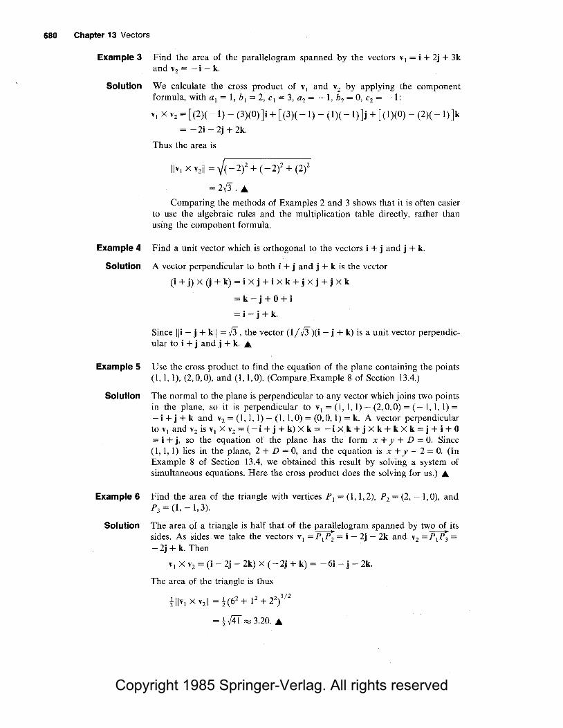
Copyright 1985 Springer-Verlag. All rights reserved
680 Chapter 13 Vectors
Example 3 Find the area of the parallelogram spanned by the vectors v 1 = i + 2j + 3k and v2 = - i - k.
Solution We calculate the cross product of v1 and v2 by applying the component formula, with a1 = 1, b1 = 2, c1 = 3, a2 = -1, b2 = 0, c2 = - 1:
v 1 X v2 = [ (2)( - 1) - (3)(0) Ji + [ (3)( - 1) - ( 1 )( - 1) Jj + [ ( 1 )(0) - (2)( - 1) J k
= - 2i - 2j + 2k.
Thus the area is
llv1 X V2ll = ~(-2)2 + ( -2)2 + (2)2
=2ff .....
Comparing the methods of Examples 2 and 3 shows that it is often easier to use the algebraic rules and the multiplication table directly, rather than using the component formula.
Example 4 Find a unit vector which is orthogonal to the vectors i + j and j + k.
Solution A vector perpendicular to both i + j and j + k is the vector
(i + j) x (j + k) = i x j + i x k + j x j + j x k
=k-j+O+i
= i - j + k.
Since Iii - j + kll =ff, the vector (l /ff )(i - j + k) is a unit vector perpendicular to i + j and j + k . .6.
Example 5 Use the cross product to find the equation of the plane containing the points (I, 1, 1), (2, 0, 0), and (1, 1, 0). (Compare Example 8 of Section 13.4.)
Solution The normal to the plane is perpendicular to any vector which joins two points in the plane, so it is perpendicular to v1 =(1,1, 1)- (2,0,0) = (-1, 1, 1) = -i + j + k and v2 =(1,1, 1)- (1, 1,0) = (0,0, 1) = k. A vector perpendicular to v1 and v2 is v1 X v2 = (-i + j + k) X k = -i X k + j X k + k X k = j + i + 0 = i + j, so the equation of the plane has the form x + y + D = 0. Since (1, 1, 1) lies in the plane, 2 + D = 0, and the equation is x + y - 2 = 0. (In Example 8 of Section 13.4, we obtained this result by solving a system of simultaneous equations. Here the cross product does the solving for us.) .6.
Example 6 Find the area of the triangle with vertices P 1 = (I, 1, 2), P 2 = (2, - 1, 0), and P3 =(I, - 1, 3).
Solution The area of a triangle is half that of the parallelogram spanned by two of its '---------+ --sides. As sides we take the vectors v1 =P1P2 = i - 2j - 2k and v2 =P1P3 =
-2j + k. Then
V1 X V2 = (i - 2j - 2k) X (-2j + k) = -6i - j - 2k.
The area of the triangle is thus
f llv1 X v2JI = t(62 + 12 + 22) I/2
= t [<IT~ 3.20 .....

Copyright 1985 Springer-Verlag. All rights reserved
13.5 The Cross Product 681
Example 7 Prove the algebraic rule 3 by using the component formula.
Solution Let v; = a;i + bj + c;k (i = 1, 2, 3). Then
and
V2 + V3 = ( G2 + G3)i + ( b2 + b3)j + ( C2 + C3)k
v, x (v2 + V3) = [ b,( C2 + C3) - c,( b2 + b3) Ji
+ [ c1(a2 + a3) - a1(c2 + c3)]j + [ a1(b2 + b3) - b1(a2 + a3)]k
= (b 1c2 - c1b2)i + (c 1a2 - a 1c2)j + (a 1b2 - b1a 2)k
+ (b 1c3 - c1b3)i + (c 1a3 - a 1c3)j + (a 1b3 - a3b1)k
=v1 Xv2 +v1 Xv3 . .A
Example 8 Show that llu X vll 2 = llull 2 llvll 2 - (u • v)2
•
Solution Let (} be the angle between u and v. Then
llu Xvii= llnll llvllsinB and u • v = llull llvllcosB.
Squaring both equations and summing gives
llu X vll 2 + (u • v)2 = llull 2 llvll\sin2B + cos2B)
= llull 2 llvll2
,
so llu X vll 2 = llull 2llvll 2 - (u • v)2. .A
Exercises for Section 13.5 Calculate the cross products in Exercises 1-10.
I. (i - i + k) x G - k). 2. ix G - k). 3. (i + j) x [(k - j) + (3j - 2i + k)]. 4. (ai + j - k) Xi. 5. [(3i + 2j) x 3j] x (2i - j + k). 6. (i x j) x (i + j + k). 7. (i+ 2j + 3k) x (i + 3k). 8. (i + j + k) x (i + k). 9. (i + k) x (i + j + k).
10. (3i - 2k) x (3i - j - k). Find the area of the parallelogram spanned by the vectors in Exercises 11-14.
11. i - 2j + k and i + j + k. 12. i - j and i + j. 13. i and i - 2j. 14. i - j - k and i + j + k.
Find a unit vector orthogonal to the pairs of vectors in Exercises 15-18.
15. i and i + j + k. 16. i - j and i + j. 17. i - j - k and 2i - 2j + k.
18. i + 2j + k and 3i - j.
19. Find a unit vector perpendicular to i + j and to i - j -- -,J:k and with a positive k component.
20. Find a unit vector perpendicular to i - j and to i + k and with a positive k component.
21. Find the equation of the plane passing through the points (0, 0, 0), (2, 0, - 1 ), and (0, 4, - 3).
22. Find the equation of the plane through the points (1,2,0), (0, 1, -2), and (4,0, 1).
23. Find the equation of the plane through (1, 1, 1) and containing the line which is the intersection of the planes x - y = 2 and y - z = I.
24. Find the equation of the plane through the point (2, 1, 1) and containing the line x = t - 1, y = 2t + 1, z = - t - I.
25. Find the area of the triangle whose vertices are (0, 1, 2), (3, 4, 5), and (-1, - 1, 0).
26. Find the area of the triangle whose vertices are (0, 1, 2), (1, 1, 1), and (2, I, 0).
27. Find the area of the triangle whose vertices are (0,0,0), (0, -1, 1), and (0, 1, -1).
28. Find the area of the triangle whose vertices are (-1, -1, -1), (-1,0, 1), and (1,0, -1).
29. Prove algebraic rule 5 by using the component formula.
30. Prove the formula in Example 8 by using the component formula.
31. By using the cross product of the vectors cos Bi + sin Bj and cos fi + sin fj, verify that sin(B - if)= sinBcosf- cosBsinf.

Copyright 1985 Springer-Verlag. All rights reserved
682 Chapter 13 Vectors
32. Let! be a line through a point P0 in direction d. Show that the distance from a point P to ! is given by l(Poh X dll/lldll·
33. Let a line in the plane be given by the equation ax+ by= c. Use the cross product to show that the distance from a point P = (x, y) to this line is given by
lax+ by- cl
..,/a2 + b2
34. Use the cross product to find a solution of the following simultaneous equations: x + y = 0 and x - y- 2z = 0.
35. In mechanics, the moment M of a force F about a point 0 is defined to be the magnitude of F times the perpendicular distance d from 0 to the line of action of F. The vector moment M is the vector of magnitude M whose direction is perpendicular to the plane of 0 and F, determined by the right-hand rule. Show that M = R x F, where R is any vector from 0 to the line of action of F. (See Fig. 13.5.6.)
0
line of action Figure 13.5.6. Moment of a force.
36. The angular velocity n of rotation of a rigid body has direction equal to the axis of rotation and magnitude equal to the angular velocity in radians per second. The sense of n is determined by the right-hand rule. (a) Let r be a vector from the axis to a point P
on the rigid body. Show that the quantity v = n X r is the velocity of P, as in Fig. 13.5.1, with g = V1 and r = V2·
(b) Interpret the result for the rotation of a carousel about its axis, with P a point on the circumference.
37. Two media with indices of refraction n1 and n2
N Light ray
Figure 13.5.7. Snell's law.
are separated by a plane surface perpendicular to the unit vector N. Let a and b be unit vectors along the incident and refracted rays, respectively, their directions being those of the light rays. Show that n1(N X a)= n2(N X b) by using Snell's law sin8ifsin82 = n2/n 1, where 81and82 are the angles of incidence and refraction, respectively. (See Fig. 13.5.7.)
* 38. Prove the following: (a) (u xv)· (ax b) = (u · a)(v · b) - (v · a)(u · b). (b) The Jacobi identity:
(u xv) x w + (v x w) Xu+ (w x u) Xv= 0.
*39. (a) Using vector methods, show that the distance between two nonparallel lines 11 and 12
is given by
l(v2 - v1) · (a1 X a2)I d=--------
lla1 X a2ll '
where v1, v2 are vectors from the origin to points on 11 and 12 , respectively, and a1 and a2 are the directions of 11 and 12 • [Hint: Consider the plane through 12 which is parallel to 11• Show that (a1 X a2)/lla1 X a211 is a unit normal for this plane; now project v2 - v1 onto this normal direction.]
(b) Find the distance between the line 11 determined by the two points (-1, -1, 1) and (0, 0, 0) and the line 12 determined by the points (0, - 2, 0) and (2, 0, 5).
*40. Use properties of the cross product to explain why, in the discussion of rotation at the beginning of this section, the resulting vector v does not depend on. the choice of the origin O; i.e., what happens if 0 is replaced by another point O' on the axis of rotation?
*41. When a gyroscope rotating about an axis n, as in Fig. 13.5.8, is subject to a force F, the gyroscope responds by moving in the direction n X F. 5
Show that this fact is consistent with the gyroscopic precession you actually observe in toy gyroscopes.
Figure 13.5.8. Gyroscope and cross products ..
5 This relationship is easiest to see in an orbiting earth satellite, where the effects of gravity do not complicate the issue. Indeed, the Skylab astronauts had great fun carrying out such experiments. (See Henry S. Cooper, Jr., A House in Space, Holt, Rinehart, and Winston, 1976).

Copyright 1985 Springer-Verlag. All rights reserved
13.6 Matrices and Determinants 683
13.6 Matrices and Determinants
(b) a1b2 -b1a2 < 0
Figure 13.6.1. ·The sign of a1b2 - b1a2 determines the orientation of the ordered pair (a1i + b1j, a2i + b2 j).
The cross product can be expressed as a 3 X 3 determinant.
From the point of view of geometry and vectors, we will consider, in turn, 2 X 2 determinants and matrices, and then the 3 X 3 case.
If v1 = a 1i + bd and v2 = a 2i + b2j are vectors in the plane, to compute the area of the parallelogram spanned by v1 and v2 , we may consider them as vectors in space (with c 1 = c2 = 0) and take the cross-product v1 X v2
= (a 1b2 - b1a2)k. The area is then [[v 1 X v2 [[ = la 1b2 - b1a21, but the sign of a1b2 - b1a2 also gives us some information: it is positive if the sense of (shortest) rotation from v1 to v2 is counterclockwise and negative if the sense of rotation is clockwise (see Fig. 13.6.1). We may say that the sign of a1b2 - b1a2 determines the orientation of the ordered pair of vectors (v1, v2).
The combination a1b2 - b1a2 of the four numbers ap b1, a2 , and b2 is denoted by
la, b, I a2 b1
and is called the determinant of these four numbers.
2 x 2 Determinants If a, b, c, d are any four numbers, we write
I~ ~I= ad- be.
The absolute value of
equals the area of the parallelogram spanned by the vectors v = ai + bj and w = ci + dj. The sign of
gives the orientation of the pair (v, w).
Example 1 (a) Find the determinant I ;1; ~I·
(b) Show that I; ~I = I! ~I = I~ : I· What is their common value?
(c) Prove that I~ ~I= -1 ~ ~I (the two columns are interchanged).
Solution (a)

Copyright 1985 Springer-Verlag. All rights reserved
684 Chapter 13 Vectors
(b) I j ~I= (1)(4) - (2)(3) = -2;
I! ~I= (1)(6)- (2)(4) = -2;
I~ :1= (1)(6) - (4)(2) = -2.
Their common value is - 2.
( c) j ~ ~I = ad - be, and
-1 ~ ~ I = - (be - ad) = ad - be. JI..
From the previous section we recall that
(a 1i + bd + c1k) X (a2i + b2j + c2k)
= (b1 c2 - c1 b2 )i + (c 1 a 2 - a 1 c2 )j + (a1 b2 - b1 a2 )k.
All the components on the right-hand side are determinants. We have:
(a 1i + bd + c1k) X (a2i + b~ + c2k)
'
b 1 c1,. lc 1 a1
,. 'a 1 = I+ J +
b2 C2 C2 a2 a2 bl I k. b2
The middle term can also be written
_,al Cl ,j. a2 C2
(1)
Shortly we shall see how to write the cross product in terms of a single 3 X 3 determinant.
Sometimes we wish to refer to the array
a b c d
of numbers without taking the combination ad - be. In this case, we use the notation
[ ~ ~] and refer to this object as a 2 X 2 matrix. Two matrices are considered equal only when all their corresponding entries are equal; thus, in contrast to the equalities in Example l(b), the matrices
[ ! ~ l are all different. The determinant
is a single number obtained by combining the four numbers in the matrix
Geometrically, we may think of a matrix as representing a parallelogram (that is, a geometric figure), while the determinant represents only the area of the parallelogram (that is, a number).

Copyright 1985 Springer-Verlag. All rights reserved
13.6 Matrices and Determinants 685
Example 2 The transpose of a matrix [ ~ ~ J is defined to be the matrix [ ~ ~ J
obtained by reflection across the main (upper left to lower right) diagonal.
(a) Find the transpose of [ I 5 ]· - 3 2
(b) Show that the determinant of a matrix is equal to the determinant of its
transpose: I~ ~I= j~ ~I· (c) Check (b) for the matrix in (a).
Solution (a) The transpose of [ _ ; ~ J is [; - ~ l
Figure 13.6.2. The absolute value of a determinant equals the volume of the parallelepiped spanned by the rows.
0
Figure 13.6.3. The volume of the parallelepiped is its height I PQ I times the area of its base.
(b)
(c)
I~ ~j=ad-bc=I~ ~I·
I l 5 1=2+15=17· - 3 2 '
1; -~1=2+ 15= 17 ....
A 3 x 3 matrix consists of nine numbers in a square array, such as
[
1 4 0 2 3 I
~ ]· -5
a1 b1 c1 a1 b1 C1
To define the determinant D = a2 b2 c2 of a 3 X 3 matrix a2 b2 c2 ,
03 b3 C3 03 b3 C3
we proceed by analogy with the 2 x 2 case. The rows of the matrix give us three vectors in space:
v 1 = a 1i + bd + c 1k,
v2 = a2i + b2j + c2k,
V3 = a3i + b3j + c 3k.
Since the determinant of a 2 x 2 matrix represents an area, we should define the determinant in such a way that its absolute value is the volume of the parallelepiped spanned by v1, v2 , and v3 . (See Fig. 13.6.2.)
To compute this volume in terms of the nine entries in the matrix, we drop a perpendicular PQ from the tip of v3 to the plane spanned by v1 and v2 •
It is a theorem of elementary solid geometry that the volume of the parallelepiped is equal to the length of PQ times the area of the parallelogram spanned by v1 and v2 (see Fig. 13.6.3).
Looking at the right angle OQP, we find that the length of PQ is llv3 ll lcos0j, where 0 is the angle between v3 and PQ. On the other hand, PQ is perpendicular to v1 and v2 , so it is parallel to v1 x v2 , so 0 is also the angle between v3 and v1 X v2 . Now we have:

Copyright 1985 Springer-Verlag. All rights reserved
686 Chapter 13 Vectors
Example 3
Volume= (area of base)(height)
= llv 1 X V2ll llv3il lcos 0 I
=I llv1 X V2il llv3llcosOI
= l(v1 X v2) · v3I·
Since the volume is to be the absolute value of the determinant, we define the determinant to be the expression inside the bars:
al bl C1
a2 b2 c2 = [ ( a 1i + b1j + c1k) X (a2 i + b2j + c2k) J • ( a 3i + b3j + c3k).
a3 b3 C3
By using the component formula for the cross product in equation (1), we find
:: !: :: =\b1 C1\a3+1c1 a11b3+1a1 b11c3 b
b2 C2 C2 a2 a2 b2 a3 3 C3
or
(2)
We take equation (2) as the definition of the determinant of a 3 x 3 matrix; the volume of the parallelepiped spanned by three vectors is thus equal to the absolute value of the determinant of the matrix whose rows are the components of the vectors. The sign of the determinant is interpreted geometrically in Example 9.
0 Evaluate the determinant 2
3
0 4 -1 6-
1 2
Solution By equation (2),
0 0 4 2 - 1 6 =I 0 41(3) -10 41< 1) +I 0 - 011(2) 3 l 2 -1 6 2 6 2
= (4)(3)- (-8)(1) + (0)(2)
= 12 + 8 = 20 ....
We can express the cross product of two vectors as a single 3 X 3 determinant. In fact, comparing equation (2), with (1),
al b1 C1
(a1i + bd + c1k) X (a2i + b2j + c2k) = a2 b2 c2 j k
(3)
Example 4 Write (i + k) X (j - 2k) as a determinant.
Solution 1 0
(i + k) x (j - 2k) = 0 1 j
1 -2 ....
k
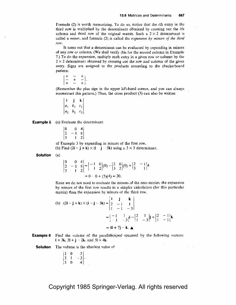
Copyright 1985 Springer-Verlag. All rights reserved
13.6 Matrices and Determinants 687
Formula (2) is worth memorizing. To do so, notice that the ith entry in the third row is multiplied by the determinant obtained by crossing out the ith column and third row of the original matrix. Such a 2 X 2 determinant is called a minor, and formula (2) is called the expansion by minors of the third row.
It turns out that a determinant can be evaluated by expanding in minors of any row or column. ry.I e shall verify this for the second column in Example 7.) To do the expansion, multiply each entry in a given row or column by the 2 x 2 determinant obtained by crossing out the row and column of the given entry. Signs are assigned to the products according to the checkerboard pattern:
I~ + ~I· (Remember the plus sign in the upper left-hand corner, and you can always reconstruct this pattern.) Thus, the cross product (3) can also be written
j k a1 b1 c1
a1 b1 C1
Example 5 (a) Evaluate the determinant
0 0 4 2 - 1 6 3 1 2
of Example 3 by expanding in minors of the first row. (b) Find (2i - j + k) X (i - j - 3k) using a 3 X 3 determinant.
Solution (a)
= 0 - 0 + (5)(4) = 20.
Since we do not need to evaluate the minors of the zero entries, the expansion by minors of the first row results in a simpler calculation (for this particular matrix) than the expansion by minors of the third row.
i j k (b) (2i - j + k) x (i - j - 3k) = 2 - I I
I - I -3
=1-1 - 1 I Ii -12 - 3 I I \i + 12 - 3 I
- l lk - I
= 4i + 7j- k ...
Example 6 Find the volume of the parallelepiped spanned by the following vectors: i + 3k, 2i + j - 2k, and Si + 4k.
Solution The volume is the absolute value of
I 0 3 2 I - 2 5 0 4

Copyright 1985 Springer-Verlag. All rights reserved
688 Chapter 13 Vectors
If we expand this by minors of the second column, the only nonzero term is
11 !1(1)= -11,
so the volume equals 11. _.
To prove that the expansions by minors of rows or columns all give the same result, it is sufficient to compare these expansions for the "general" 3 X 3 determinant.
Example 7 Show that expanding the determinant
al bl C1
a2 b2 C2
a3 b3 C3
by minors of the second column gives the correct result.
Solution The expansion by minors of the second column is
-1a2 c2lb1 + la1 C1 lb2 -1a1 C1 lb3. a3 C3 a3 C3 a2 C2
Expanding the 2 x 2 determinants gives
-( a 2c3 - c2a 3)b 1 + ( a 1c3 - c 1a 3)b2 - ( a 1c 2 - c1a 2)b3
= - b 1a 2c3 + b 1c2a 3 + a 1b 2c3 - c 1b 2a 3 - a 1c2b 3 + c1a 2b 3 .
Collecting the terms in a 3 , b 3 , and c 3 , we get
( b 1c 2 - c 1b 2)a3 - ( a 1c 2 - c 1a 2)b3 + ( a 1b 2 - b 1a 2)c3
=lb! b2
C1 la3 -1a1 C2 a2
Cl lb3 +la! C2 a2
bl I b2
C3
a1 bl Cl
a2 b2 C2 ... a3 b3 C3
The proof that we get the same result by expanding in any row or column is similar.
If V1 = a1i + b1i + C1k, V2 = a2i + b2j + C2k, and V3 = a3i + b3j + C3k, equation (2) can be written
al bl Cl
a2 b2 C2 = (v1 x V2). V3.
a3 b3 C3
This is called the triple product of v1, v2, and v3.
Example8 Show that (v1Xv2)·v3 =(v3 Xv1)·v2. In fact, the numbers 1,2,3 can be moved cyclically without changing the value of the triple product:
r 1 :.-3 2
Solution The triple product (v3 X v1) • v2 is equal to the determinant
a3 b3 C3
al bl Cl
a2 b2 C2

Copyright 1985 Springer-Verlag. All rights reserved
13.6 Matrices and Determinants 689
Expanding this by minors of the first row gives
Expanding the determinant for (v1 x v2) • v3 by the third row gives the same result. ...
Example 9 Let v1 = a 1i + b1j + c1k, v2 = a2i + b2 j + c2k, and v3 = a3i + b3j + c3k. Show that the triple (v 1' v2 , v3) is right-handed (left-handed) if the determinant
al bl Cl
a2 b2 C2
a3 b3 C3
is positive (negative). What does it mean if the determinant is zero?
Solution Let 9 be the plane spanned by v1 and v2 • (We assume that v1 and v2 are not parallel; otherwise v1 X v2 = 0, and the determinant is zero.) Then (v1, v2 , v3) is right handed (left handed) if and only if v3 lies on the same (opposite) side of 9 as v1 X v2 ; that is, if and only if (v1 X v2) • v3 is positive (negative); but (v1 X v2) • v3 is the determinant
al bl Cl
a2 b2 C2
a3 b3 C3
If the determinant is zero (but v1 X v2 is not zero), then v3 must lie in the plane 9. In general, we may say that the determinant is zero when the vectors v 1, v 2 , and v 3 fail to span a solid parallelepiped, but instead lie in a plane, lie on a line, or are all zero. Such triples of vectors are said to be linearly dependent and are neither right-handed nor left-handed . .&
3 x 3 Determinants
The determinant can be expanded by minors of any row or column. If
v1 = a 1i + bJi + c1k,
V2 = a2i + b2j + C2k,
v3 = a3i + b3 j + c3k,
then the determinant equals (v1 X v2) • v3 which is also called the triple product of v1, v2 , and v3 .
The absolute value of the determinant equals the volume of the parallelepiped spanned by v1 , v2 , and v3 •
The sign of the determinant tells whether the triple (v1 , v2 , v3) is right- or left-handed.

Copyright 1985 Springer-Verlag. All rights reserved
690 Chapter 13 Vectors
Exercises for Section 13.6 Evaluate the determinants in Exercises 1-10.
1. 1- ~ ~ I 2. 1-~ ~I
3. I 6 1~1 4. I~ 1°1 I 12
5. 1 3 ~I 6.
Ii ~I 7. 4 8.
1 ~I 11 ~ x - 1 I -1-x
9. I~ ~I 10. 1-% ~I
Prove the identities in Exercises 11-14.
11. I~ ~I = -1 ~ ~I (the two rows are interchanged).
12. I~ ~I= la; c b; di (the last row is added to
the first).
13 I rca rdb I = 'I ac b I ( h f' . 1 . l' d b · d t e lfst row is mu tip ie y
a constant).
14. I a - sb b I =I a b I (a constant times the sec-c - sd d c d
ond column is subtracted from the first). Evaluate the determinants in Exercises 15-24.
15.16 ~ 61 16.16 ~1 1 0 1 0 1
17.1~ - ~ ~1 18. Ii -~ ii 3 0 1 1 0 0
19.1- ~ _ i ~I 20.1-i ~ ~I 0 1 -1 0 1 2
21. I~ ~ ~I 22
· l-i ~ ~I 23
· I~ ~ II 24· I~ ~ ~I
Write the cross products in Exercises 25-30 as determinants and evaluate.
25. (3i - j) x G + k). 21. (i + j) x G + k). 29. (i - k) x (i + k).
26. (i + 3j - k) x (i - 3j + k). 28. (2i + 4j + 6k) x k. 30. G + 2k) x (32j + 64k).
31. Find the volume of the parallelepiped spanned by the vectors i + j + k, i - j + k, and 3k.
32. Find the volume of the parallelepiped spanned by i - j, j - k, and k + i.
33. Find the volume of the parallelepiped with one vertex at (1, 1, 2) and three adjacent vertices at (2, 0, 2), (3, 1, 3), and (2, 2, - 3).
34. Find the other four vertices of the parallelepiped in Exercise 33 and use them to recompute the volume.
35. Check that expanding the determinant
al bl C1
a2 b2 C2
a3 b3 C3
by (a) minors of the second row and (b) minors of the third column gives the correct result.
36. Show that if the first two rows of a 3 X 3 matrix are interchanged, the determinant changes sign.
37. Show that if the first two columns of a matrix are interchanged, the determinant changes sign.
38. Use Exercise 36 to verify that (v 1 X v2) • v3 = -(v2 Xv1)·v3.
39. Verify that (v1 X v2) • v3 = (v2 X v3) • v1. 40. Verify that (v1 - v2) X (v1 + v2) = 2v1 X v2 .
41. Show by drawing appropriate diagrams that if (v1, v2 , v3) is a right-handed triple, then so is (v2, V3, V1)·
42. Show that if two rows or columns of .1 3 X 3 matrix are equal, then the determinant of the matrix is zero.
43. Show that if
I~ ~1* 0, then the solutions to the equations
ax+ by= e,
ex+ dy = f are given by the formulas
This result is called Cramer's rule6 (We have already used it without the language of determinants in our discussion of Wronskians in the Supplement to Section 12.7.)
44. Use Cramer's rule (Exercise 43) to solve the equations 4x + 3y = 2; 2x - 6y = 1.
*45. Suppose that the determinant
al b1 C1
D = a2 b2 c2 a3 b3 C3
6 Gabriel Cramer (1704-1752) published this rule in his book, Introduction a !'analyse des lignes courbes algebriques (1750). However, it was probably known to Maclaurin in 1729. For systems of n equations inn unknowns, there is a generalization of this rule, but it can be inefficient to use on a computer when n is large. (See Exercises 45 for the case n = 3.)

Copyright 1985 Springer-Verlag. All rights reserved
is unequal to zero. Show that the solution of the equations
G1X + h1J + C1Z = d1,
GzX + bzy + CzZ =dz,
G3X + b3y + C3Z = d3
is given by the formulas
d1 b1 CJ
dz bz Cz
d3 b3 C3 x=
D
a1 b1 d1
Gz hz dz
a3 b3 d3 z=
D
a1 d1 CJ
Gz dz Cz
G3 d3 C3 y=
D
This result is called Cramer's rule for 3 X 3 systems.
46. Use Cramer's rule (Exercise 45) to solve
-x+y =14, 2x+y + z = S, x+y+5z=-l.
Use Cramer's rule to solve the systems in Exercises 47 and 4S.
47. 2x + 3y = 5; 3x - 2y = 9. 4S. x + y + z = 3; x - y + z = 4; x + y - z = 5.
49. Check that
a d g b e h
c f
a b c d e f. g h
That is, check that the determinant of the transpose of a 3 x 3 matrix is equal to the determinant of the original matrix.
*50. Show that adding a multiple of the first row of a
Review Exercises for Chapter 13 Complete the calculations in Exercises 1-16.
I. (3, 2) + ( - 1, 6) =
2. 2(1, -4) + (1,5) =
3. (1,2,3) + 2(-1, -2, 7) = 4. 2[(-1,0, 1) + (6,0,2)]- (0,0, 1) = 5. (3i + 2j) + (Si - j - k) = 6. (Si + 3j - k) - 6(i - j - k) = 7. (Si+ 3j - k) x (i - j - k) =
S. (i - j - k) . (i + j + 2k) = 9. (Si + 3j - k) · (i - j - k) =
10. (i+ j) . (i - j) =
11. (i + j) x (i - j) = 12. [(2i - j) x (3i + j)]. (2j + k) = 13. u Xv=?, where u = 2i + j and v = k. 14. u · v = ?, where u = 3j - k and v = 2j + i. 15. u - 3v = ?, where u and v are as in Exercise 13. 16. u + 6v = ?, where u and v are as in Exercise 14.
Review Exercises for Chapter 13 691
matrix to the second row leaves the determinant unchanged; that is,
al b1 C1
az bz Cz
G3 b3 C3
[In fact, adding a multiple of any row (column) of a matrix to another row (column) leaves the determinant unchanged.]
*51. Justify the steps in the following computation:
I
1 2 4 5 7 s ~ 1=1
6 10 7
=I~ =1-3
-6
2 -3 s 2
-3 -6
3 I -6 - 11
- 6 1=33-36= -3. - 11
*52. Follow the technique of Exercise 51 to evaluate the determinant
I I 2 51 2 3 6 .
- 1 2 1
(Add - 2 times the first row to the second row, then add the first row to the third row.)
*53. Use the technique in Exercise 51 to evaluate the 3 X 3 determinants in Exercises lS and 19.
*54. Show that the plane which passes through the three points A = (a I> az, a3), B = ( b1, bz, b3), and C = (c1> Cz, c 3) consists of the points P = (x, y, z) given by
a1 - x az - y a3 - z
b1 - x bz - y b3 - z = 0. C1 - X Cz - J C3 - Z
[Hint: Write the determinant as a triple product.]
17. Find a unit vector orthogonal to 3i + 2k and j- k.
lS. Find a unit vector orthogonal to j + k and 2i + k. 19. Find the volume of the parallelepiped spanned
by 2i - j + k, i, and j - k. 20. Find the volume of the parallelepiped spanned
by i + j, i - j, and i + k. 21. (a) Draw the vector v joining (-2, 0) to (4, 6) and
find the components of v. (b) Add v to the vector joining ( - 2, 0) to (I, I).
22. Find the intersection of the medians of the triangle with vertices at (0, 0), ( 1, n and (2, 0).
23. Let PQR be a triangle in the plane. For each side of the triangle, construct the vector perpendicular to that side, pointing into the triangle, and having the same length as the side. Prove that the sum of the three vectors is zero.
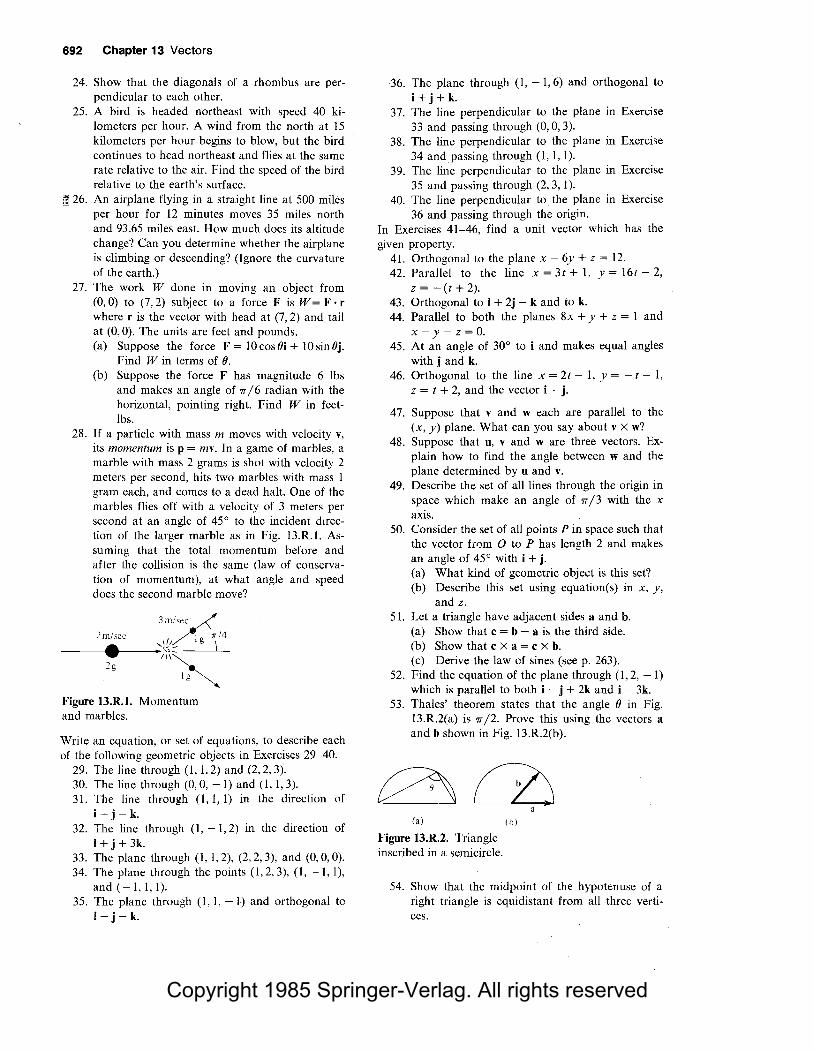
Copyright 1985 Springer-Verlag. All rights reserved
692 Chapter 13 Vectors
24. Show that the diagonals of a rhombus are perpendicular to each other.
25. A bird is headed northeast with speed 40 kilometers per hour. A wind from the north at 15 kilometers per hour begins to blow, but the bird continues to head northeast and flies at the same rate relative to the air. Find the speed of the bird relative to the earth's surface.
rul 26. An airplane flying in a straight line at 500 miles per hour for 12 minutes moves 35 miles north and 93.65 miles east. How much does its altitude change? Can you determine whether the airplane is climbing or descending? (Ignore the curvature of the earth.)
27. The work W done in moving an object from (0, 0) to (7, 2) subject to a force F is W = F · r where r is the vector with head at (7, 2) and tail at (0, 0). The units are feet and pounds. (a) Suppose the force F = 10 cos Bi+ 10 sin Bj.
Find Win terms of B. (b) Suppose the force F has magnitude 6 lbs
and makes an angle of 7T /6 radian with the horizontal, pointing right. Find W in feetlbs.
28. If a particle with mass m moves with velocity v, its momentum is p = mv. In a game of marbles, a marble with mass 2 grams is shot with velocity 2 meters per second, hits two marbles with mass 1 gram each, and comes to a dead halt. One of the marbles flies off with a velocity of 3 meters per second at an angle of 45° to the incident direction of the larger marble as in Fig. 13.R. l. Assuming that the total momentum before and after the collision is the same (law of conservation of momentum), at what angle and speed does the second marble move?
2m/sec
3m/sec _/
,,,/g ~/4 ----t·I-----... ''":.- ----'---. ;'"""
2g ' 1 g ""'
Figure 13.R.1. Momentum and marbles.
Write an equation, or set of equations, to describe each of the following geometric objects in Exercises 29-40.
29. The line through (I, I, 2) and (2, 2, 3). 30. The line through (0, 0, -1) and (1, 1, 3). 31. The line through ( 1, 1, 1) in the direction of
i-j-k. 32. The line through (I, - 1, 2) in the direction of
i + j + 3k. 33. The plane through (1, 1,2), (2,2,3), and (0,0,0). 34. The plane through the points (1,2,3), (1, -1, 1),
and ( - 1, 1, 1). 35. The plane through (1, 1, - l) and orthogonal to
i-j-k.
36. The plane through (1, - 1, 6) and orthogonal to i + j + k.
37. The line perpendicular to the plane in Exercise 33 and passing through (0, 0, 3).
38. The line perpendicular to the plane in Exercise 34 and passing through (1, 1, 1).
39. The line perpendicular to the plane in Exercise 35 and passing through (2, 3, 1).
40. The line perpendicular to the plane in Exercise 36 and passing through the origin.
In Exercises 41-46, find a unit vector which has the given property.
41. Orthogonal to the plane x - 6y + z = 12. 42. Parallel to the line x = 3t + 1, y = 16t - 2,
z = -(t + 2). 43. Orthogonal to i + 2j - k and to k. 44. Parallel to both the planes 8x + y + z = 1 and
x - y- z = 0. 45. At an angle of 30° to i and makes equal angles
with j and k. 46. Orthogonal to the line x = 2t - 1, y = - t - 1,
z = t + 2, and the vector i - j.
47. Suppose that v and w each are parallel to the (x, y) plane. What can you say about v X w?
48. Suppose that u, v and w are three vectors. Explain how to find the angle between w and the plane determined by u and v.
49. Describe the set of all lines through the origin in space which make an angle of 7T /3 with the x axis.
50. Consider the set of all points P in space such that the vector from 0 to P has length 2 and makes an angle of 45° with i + j. (a) What kind of geometric object is this set? (b) Describe this set using equation(s) in x, y,
and z. 51. Let a triangle have adjacent sides a and b.
(a) Show that c = b - a is the third side. (b) Show that c X a = c x b. (c) Derive the law of sines (seep. 263).
52. Find the equation of the plane through (1, 2, -1) which is parallel to both i - j + 2k and i - 3k.
53. Thales' theorem states that the angle B in Fig. 13.R.2(a) is 7T /2. Prove this using the vectors a and b shown in Fig. 13.R.2(b).
~CL) (a) (b)
Figure 13.R.2. Triangle inscribed in a semicircle.
a
54. Show that the midpoint of the hypotenuse of a right triangle is equidistant from all three vertices.

Copyright 1985 Springer-Verlag. All rights reserved
Evaluate the determinants in Exercises 55-62.
55. 1- ~ ii 56. I~ -: I 57. 1-i - : I 58. I-~ 61
I~ - 1
-l 1 I~ 0
r1
59. I 60. - 1 3 1
61.1 i 1 11 1-1
0 -~I 2 2 62. I 0 3 3 -1 0
63. Find the area of the parallelogram spanned by 3i - 2j + k and 8i - k.
64. Find the area of the parallelogram spanned by 2i - j and 3i - 2j.
65. Find the volume of the parallelepiped spanned by i - j ~ k, 2i + j - 5k, and ~ i - j + ! k.
66. Find the volume of the parallelepiped spanned by 2j + i, i - j, and k.
67. The volume of a tetrahedron with concurrent edges a, b, c is given by V = (1/6)a · (b x c). (a) Express the volume as a determinant.
(b) Evaluate V when a= i + j + k, b = i - j + k, c = i + j.
68. A tetrahedron sits in xyz coordinates with one vertex at (0, 0, 0), and the three edges concurrent at (0, 0, 0) are coincident with the vectors a, b, c.
(a) Draw a figure and label the heads of the vectors as a, b, c.
(b) Find the center of mass of each of the four triangular faces of the tetrahedron.
69. Let r1, ..• , rn be vectors from 0 to the masses m 1 , ••• , mn. The center of mass is the vector
70.
71.
72.
c = ( _± m;r;) / ( ± m;) 1=! 1=!
Show that for any vector r,
n n
L m;/lr- r;ll 2 = L m;llr;- cll 2 + mllr - cll 2
, i=l
where m = 2,7= 1m; is the total mass of the system.
Solve the following equations using Cramer's rule (Exercise 43, Section 13.6): x + y = 2; 3x - y = 4.
Solve by using determinants (Exercise 45, Section 13.6): x-y+2z=4; 3x+y+z=l; 4x - y - z = 2.
Use Exercise 50, Section 13.6 to show that
2i~ I = I ~~ ~~~ 1 2 - I
2471 23 . 1
Review Exercises for Chapter 13 693
73. Evaluate
1
6 2 2 2 4 8
-~1 -1
using Exercise 50, Section 13.6. 74. Use Exercise 50, Section 13.6 to show that
I n n+l n+21
n+3 n+4 n+5 n+6 n+7 n+8
has the same value no matter what n is. What is this value?
75. Show that for all x, y, z,
x+2 y z y + 1 5 5
z ly 10 = - I 2 5
x+2 z-x-2
5 10; zl
76. Show that
x x 2
Y Y2 *o z z 2
if x, y, and z are all different. 77. If the triple product (v X j) · k is zero, what can
you say about the vector v? 78. Suppose that the three vectors a;i + b;j + c;k for
i = 1, 2, and 3 are unit vectors, each orthogonal to the other two. Find the value of
al bl C1
a2 b2 C2
a3 b3 C3
79. A sphere of radius 10 centimeters with center at (0, 0, 0) rotates about the z axis with angular velocity 4 radians per second such that the rotation looks counterclockwise from the positive z axis.
80.
(a) Find the rotation vector 0 (see Section 13.5, Exercise 36).
(b) Find the velocity v =ax r when r = 5/f (i - j) is on the "equator."
A pair of dipoles are located at a distance r from each other. The magnetic potential energy P is given by P = - m 1 • B2 (dipole-dipole interaction potential), where the first dipole has moment m1
in the external field B2 of the second dipole. In MKS units,
- m2 + 3(m2 • qt, B2 = /to--------
4'1Tr3
where 1, is a unit vector, and µ0 1s a scalar constant. (a) Show that
rn 1 ·m2 -3(m2 ·1,)(m1 ·1,) P = µo 3 ·
4nr
(b) Find P when m1 and m2 are perpendicular.

Copyright 1985 Springer-Verlag. All rights reserved
694 Chapter 13 Vectors
81. (a) Suppose that v · w = 0 for all vectors w. Show that v = 0. [Note: This is not the same thing as showing that 0 · w = O.]
(b) Suppose that u • w = v · w for all vectors w. Show that u = v.
(c) Suppose that v · i = v · j = v · k = 0. Show that v = 0.
(d) Suppose that u · i = v · i, u · j = v · j, and u · k = v · k. Show that u = v.
82. Let A, B, C, D be four points in space. Consider the tetrahedron bounded by the four triangles 6 1 =BCD, 6 2 = ACD, 6 3 = ABD, and 6 4 =ABC. The triangle 6; is called the ith face of the tetrahedron. For each i, there is a unique vector v; defined as follows: V; is perpendicular to the face 6; and points into the tetrahedron; the length of V; is equal to the area of 6;. (a) Prove that for any tetrahedron ABCD, the
sum v1 + v2 + v2 + v4 is zero. [Hint: Use algebraic properties of the cross-product.]
*(b) Try to generalize the result of part (a) to more complicated polyhedra. (A polyhedron is a solid which is bounded by planar figures.) In other words, show that the sum of the inward normals, with lengths equal to areas of the sides, is zero. You may want to do some numerical calculations if you cannot prove anything, or you may want to restrict yourself to a special class of figures (distorted cubes, decapitated tetrahedra, figures with five vertices, and so forth).
* (c) There is a physical interpretation to the results in parts (a) and (b). If the polyhedron is immersed in a fluid under constant pressure p, then the force acting on the ith face is pv;. Interpret the result 2;v; = 0 in this context. Does this contradict the fact that water pressure tends to buoy up an immersed object? [Note: There is a version of all this material for smooth surfaces. It is related to a result called the divergence theorem and involves partial differentiation and surface integrals. See Chapter 18.]
83. Let P = (1, 2) and Q = (2, 1). Sketch the set of points in the plane of the form rP + sQ, where r ands are: (a) positive integers; (b) integers; (c) positive real numbers; (d) real numbers.
84. Repeat Exercise 83 with P =(I, 2) and Q = (2, 4).
*85. Repeat Exercise 83 using the points P =(I, 2) and Q = ( 7T, 27T). (You may have to guess parts (a) and (b).)
* 86. There are two unit vectors such that if they were
x
drawn on the axes of Fig. 13.R.3, their heads and tails would appear to be at the same point (that is, they would be viewed head on). Approximately what are these vectors? [Hint: Suppose that when you tried to plot a point P, the resulting dot on the paper fell right where the axes cross.]
z
y
Figure 13.R.3. Which unit vectors would be drawn as the dot at the orign?
*87. A regular tetrahedron is a solid bounded by four equilateral triangles. Use vector methods to find the angle between the planes containing two of the faces.
*88. In integrating by partial fractions, we are led to the problem of expressing a rational function
C2X2 + C1X + Co
as a sum
a2 a2 a3 --·+--+-x - r1 x - r2 x - r3
(a) Show that the undetermined coefficients a 1,
a2 , a3 satisfy a system of three simultaneous linear equations.
(b) Applying Cramer's rule (Exercise 45, Section 13.6) to this system, show that the determinant D is equal to
I r2 l r3 r3 l r1 r1 l r2 I· r2r3 r3r1 r1 rz
(c) Evaluate the determinant in (b) and show that it is nonzero whenever r 1, r2 , and r3 are all different.
(d) Conclude that the decomposition into partial fractions is always possible if r 1, r2 , and r 3 are all different.
(e) What happens if r 1 = r 2? Give an example. *89. Read Chapter 5 of Friedrichs' book, From
Pythagoras to Einstein (Mathematical Association of America, New Mathematical Library, 16 (1965)) on the application of vectors to the study of elastic impacts, and prepare a two-page written report on your findings.

Copyright 1985 Springer-Verlag. All rights reserved
Chapter14
Curves and Surfaces
Some three-dimensional geometry is needed for understanding functions of two variables.
The main subject of this chapter is surfaces in three-dimensional space. In preparation for this, we begin with a study of some special curves in the plane -the conic sections. In the last two sections, we will do some calculus with curves in space. Applications of calculus to surfaces are given in Chapters 15 and 16.
14.1 The Conic Sections
Figure 14.1.1. Conic sections are obtained by slicing a cone with a plane; which conic section is obtained depends on the direction of the slicing plane.
All the curves described by quadratic equations in two variables can be obtained by cutting a cone with planes.
The ellipse, hyperbola, parabola, and circle are called conic sections because they can all be obtained by slicing a cone with a plane (see Fig. 14.1.1). The
v (\ /\
Hyperbola Parabola
Qo Circle Ellipse

Copyright 1985 Springer-Verlag. All rights reserved
696 Chapter 14 Curves and Surfaces
theory of these curves, developed by Apollonius of Perga (262-200 B.c.), is a masterwork of Greek geometry. We will return to the three-dimensional origin of the conics in Section 14.4, after we have studied some analytic geometry in space. For now, we will treat these curves, beginning with the ellipse, purely as objects in the plane.
Definition of Ellipse An ellipse is the set of points in the plane for which the sum of the distances from two fixed points is constant. These two points are called the foci (plural of focus).
An ellipse can be drawn with the aid of a string tacked at the foci, as shown in Fig. 14.1.2.
To find an equation for the ellipse, we locate the foci on the x axis at the points F' = ( - c, 0) and F = ( c, 0). Let 2a > 0 be the sum of the distances from a point on the ellipse to the foci. Since the distance between the foci is 2c, and the length of a side of a triangle is less than the sum of the lengths of the other sides, we must have 2c < 2a; i.e., c <a. Referring to Fig. 14.1.3, we
y
P= (x,y)
Figure 14.1.2. Mechanical construction of an ellipse.
F' = (-c, 0) F= (c,0)
Figure 14.1.3. Pis on the ellipse when IFPI + IF'PI = 2a.
see that a point P = (x, y) is on the ellipse precisely when
JFPJ + JF'PJ = 2a.
That is,
~(x + c)2 + y 2 +~(x - c)2 + y 2 = 2a.
Transposing ~( x - c )2 + y 2 , squaring, simplifying, and squaring again yields
( a2 - c2)x2 + ay2 = a2( a2 - c2).
x
Let a2 - c2 = b2 (remember that a > c > 0 and so a2 - c2 > 0). Then, after division by a 2b2
, the equation becomes
x2 y2 -+-=l. a2 b2
This is the equation of an ellipse in standard form. Since b2 = a2 - c2 < a2, we have b < a. If we had put the foci on they
axis, we would have obtained an equation of the same form with b >a; the length of the "string" would now be 2b rather than 2a. (See Fig. 14.1.4.) In either case, the length of the long axis of the ellipse is called the major axis, and the length of the short axis is the minor axis.

Copyright 1985 Springer-Verlag. All rights reserved
Figure 14.1.4. The appearance of an ellipse in the two cases b < a and b >a.
y
(a) b <a
x2 y2 -+-=I a2 b2
x
14.1 The Conic Sections 697
y
x2 y2 _ -+--1 a2 b2
x
(b) b>a
Example 1 Sketch the graph of 4x 2 + 9y2 = 36. Where are the foci? What are the major and minor axes?
Solution Dividing both sides of the equation by 36, we obtain the standard form
Figure 14.1.5. The graph of 4x2 + 9y2 = 36.
Example 2
2 y2 ~+4=1.
Hence a= 3, b = 2, and c =Va2 - b2 =VS. The foci are (±VS,O), they
intercepts are (0, ± 2), and the x intercepts are ( ± 3, 0). The major axis is 6 and the minor axis is 4. The graph is shown in Fig. 14.1.5.
y
(0,2)
(3,0) x
(0,-2)
Sketch the graph of 9x 2 + y 2 = 81. Where are the foci?
y Solution Dividing by 81, we obtain the standard form x 2 /32 + y 2 /92 = 1. The graph is sketched in Fig. 14.1.6. The foci are at (0, ± 6.,/2 ). _.
(0,9)
( 3,0) (3,0)
x
(0,-9)
Figure 14.1.6. The ellipse 9x2 +y2 =81.
Ellipse 2 l
.£ + Y2
= 1 (standard form). a 2 b
Equation:
Foci: ( ± c, 0) where c = ,/a1 - b1 if a > b.
(0, ± c) where c = ,/b2 - a 2 if a < b.
If a = b, the ellipse is a circle. x intercepts: (a, 0) and ( - a, 0). y intercepts: (0, b) and (0, - b ). If P is any point on the ellipse, the sum of its distances from the foci is 2a if b < a or 2b if b > a.

Copyright 1985 Springer-Verlag. All rights reserved
698 Chapter 14 Curves and Surfaces
Figure 14.1.7. Mechanical construction of a hyperbola.
Figure 14.1.8. Pis on the hyperbola when IF' Pl - IFPI = ±2a.
The second type of conic section, to which we now turn, is the hyperbola.
Definition of Hyperbola A hyperbola is the set of points in the plane for which the difference of
. the distances from two fixed points is constaIJ.t. These two points are called the foci.
To draw a hyperbola requires a mechanical device more elaborate than the one for the ellipse (see Fig. 14.1.7); however, we can obtain the equation in the same way as we did for the ellipse. Again let the foci be placed at F' = ( - c, 0)
and F = ( c, 0), and let the difference in question be 2a, a > 0. Since the difference of the distances from the two foci is 2a and we must have IF'PI < IFPI + IF'FI, it follows that IF'PI - IFPI < IF'FI, and so 2a < 2c. Thus we must have a< c (see Fig. 14.1.8). The point P = (x, y) lies on the
F'~(-c,0)
/ y
/
y
/ /
/
hyperbola exactly when
vex+ c)2 + y2 -vex - c)2 + y2 = ±2a.
After some calculations (squaring, simplifying and squaring again), we get
e a2 - c2)x2 + ay2 = a2e a2 - c2).
If we let c2 - a2 = b2 (since a< c), we get
x2 y2 ---=l a2 b2
which is the equation of a hyperbola in standard form. For x large in magnitude, the hyperbola approaches the two lines y =
±(b/a)x, which are called the asymptotes of the hyperbola. To see this, for x and y positive, we first solve for y in the equation of the hyperbola, ob-

Copyright 1985 Springer-Verlag. All rights reserved
Figure 14.1.9. The vertical distance d from the hyperbola to its asymptote y=(b/a)xis
~ ( x - vx2 - a2)
ab
x +vx2 - a2
14.1 The Conic Sections 699
taining y = (b / a)-/x 2 - a2
• Subtracting this from the linear function (b / a)x, we find that the vertical distance from the hyperbola to the line y = (b / a)x is given by
d = % ( x -Jx2 - a2
).
To study the behavior of this expression as x becomes large, we multiply by
(x + )x2 - a2 )/(x + )x2
- a2) and simplify to obtain ab /(x + )x2
- a2 ). As
x becomes larger and larger, the denominator increases as well, so the quantity d approaches zero,,-Thus the hyperbola comes closer and closer to the line. The other quadrants a're treated similarly. (See Fig. 14.1.9.)
y
(-c,O) / I I I// Ji--
/ /
~/ ~
/ (0,b) _/ --/l I
/I I
d
/1 I / I (c,O)
\. (a,0) (x ,0)
'- I '\,I --~
', '\ ~ ~
x
Example 3 Sketch the curve 25x2 - 16y2 = 400.
Solution Dividing by 400, we get the standard form x 2/16 - y 2 /25 = 1, so a = 4 and b = 5. The asymptotes are y = ± ix, and the curve intersects the x axis at (±4,0) (see Fig. 14.1.10). It.
5 Y =4x;:
(0,5) /
/(4,5)/ ----,(
/I /1
/,
-,/ Focus=(v'4J,Ol
' x I (4,0J I / '\ I 1/ \.I Ji---- ---~
,<-4.-5) I (4,--5) '"
I \~ -5) \. I ' ~
y ~ v ~
Figure 14.1.10. The hyperbola 25x2
- I6y 2 = 400.
y
Figure 14.1.11. A hyperbola with foci on they axis.
b y=-x a
x
If the foci are located on they axis, the equation of the hyperbola takes the second standard form y 2
/ b2 - x 2
/ a2 = 1 (see Fig. 14.1.11 ). Notice that if we draw the rectangle with (±a, 0) and (0, ± b) at the
midpoints of its sides, then the asymptotes are the lines through opposite corners, as shown in Figs. 14.1.10 and 14.1.11.

Copyright 1985 Springer-Verlag. All rights reserved
700 Chapter 14 Curves and Surfaces
Example 4 Sketch the graph of 4y2 - x 2 = 4.
Solution Dividing by 4, we get y 2 - x 2 /22 = I, which is in the second standard form
with a = 2 and b = 1. The hyperbola and its asymptotes are sketched in Fig. 14.1.12 ....
Figure 14.1.12. The hyperbola 4y2 - x 2 = 4.
Figure 14.1.13. Pis on the parabola when IPFI = IPGI.
y ,.,,.--Focus= (0,VS)
'Focus= (0,-VS)
Hyperbola Case 1: Foci on x axis Case 2: Foci on y axis
2 y2 y2 2 Equation: £ - - = 1 - - £ = I
a2 b2 b2 a2
Foci:(± c,O), c =)a2 + b2 (0, ± c), c =)a2 + b2
x intercepts: (±a, 0) none y intercepts: none (0, ± b)
Asymptotes: y = ± !z_ x y = ± !z_ x a a
If P is any point on the hyperbola, the difference between its distances from the two foci is 2a in case 1 and 2b in case 2.
We are already familiar with the circle and parabola from Section R.5. The circle is a special case of an ellipse in which a = b; that is, the foci coincide. The parabola can be thought of as a limiting case of the ellipse or hyperbola, in which one of the foci has moved to infinity. It can also be described as follows:
Definition of Parabola A parabola is the set of points in the plane for which the distances from a fixed point, the focus, and a fixed line, the directrix, are equal.
Placing the focus at (0, c) and the directrix at the line y = - c leads, as above, to an equation relating x andy. Here we have (see Fig. 14.1.13) IPFI = jPGj.
y
x y = ---c ----+------
Directrix G = (x,-c)
That is, ~x2 + (Y - c)2 = ly + cj, so x 2 + (y - c)2 = (y + c)2, which gives
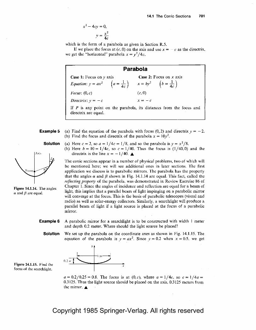
Copyright 1985 Springer-Verlag. All rights reserved
Example 5
Solution
Axis
Figure 14.1.14. The angles a and f3 are equal.
x 2 - 4cy = 0,
x2 y = 4c
14.1 The Conic Sections 701
which is the form of a parabola as given in Section R.5. If we place the focus at ( c, 0) on the axis and use x = - c as the directrix,
we get the "horizontal" parabola x = y 2 /4c.
Parabola Case 1: Focus on y axis Case 2: Focus on x axis
Equation: y = ax2 (a = 41c ) x = by2
Focus: (0, c) (c,O)
Directrix: y = - c x = -c
If P is any point on the parabola, its distances from the focus and directrix are equal.
(a) Find the equation of the parabola with focus (0, 2) and directrix y = - 2. (b) Find the focus and directrix of the parabola x = 10y2
•
(a) Here c = 2, so a= l/4c = 1/8, and so the parabola isy = x 2/8. (b) Here b = 10 = l/4c, so c = 1/40. Thus the focus is (1/40,0) and the
directrix is the line x = - 1/40. .&.
The conic sections appear in a number of physical problems, two of which will be mentioned here; we will see additional ones in later sections. The first application we discuss is to parabolic mirrors. The parabola has the property that the angles a and f3 shown in Fig. 14.1.14 are equal. This fact, called the reflecting property of the parabola, was demonstrated in Review Exercise 86 of Chapter 1. Since the angles of incidence and reflection are equal for a beam of light, this implies that a parallel beam of light impinging on a parabolic mirror will converge at the focus. This is the basis of parabolic telescopes (visual and radio) as well as solar-energy collectors. Similarly, a searchlight will produce a parallel beam of light if a light source is placed at the focus of a parabolic mirror.
Example 6 A parabolic mirror for a searchlight is to be constructed with width 1 meter and depth 0.2 meter. Where should the light source be placed?
Solution We set up the parabola on the coordinate axes as shown in Fig. 14.1.15. The equation of the parabola is y = ax2
. Since y = 0.2 when x = 0.5, we get
Figure 14.1.15. Find the focus of the searchlight.
y
0.2 m
x
a= 0.2/0.25 = 0.8. The focus is at (O,c), where a= l/4c, so c = l/4a = 0.3125. Thus the light source should be placed on the axis, 0.3125 meters from the mirror . .&.

Copyright 1985 Springer-Verlag. All rights reserved
702 Chapter 14 Curves and Surfaces
In courses in mechanics, it is shown that bodies revolving about the sun (planets, asteroids, and comets) do so in elliptic, parabolic, or hyperbolic orbits with the sun at one focus. We shall see part of the derivation of this fact in Section 14.7. Most planetary orbits are nearly circular. To measure the departure from circularity, the eccentricity is introduced. It is defined by
e = !:._, a
where a, b, and c are defined as on p. 697, with a > b. Thus a and b are the semi-major and semi-minor axes and c is the distance of a focus from the center; c = .,/a2
- b2• An ellipse is circular when e = 0, and as e approaches I,
the ellipse grows longer and narrower.
Example 7 The eccentricity of Mercury's orbit is 0.21. How wide is its orbit compared to its length?
Solution Since e = 0.21, c = 0.21a, so c2 = a 2 - b2
, and therefore b2 = a 2 - c2 =
a 2(1 - (0.21 )2) = 0.9559a2
• Hence b ~ 0.9777 a, so the orbit is 0.9777 times as wide as it is long . .&
Exercises for Section 14.1 I. Sketch the graph of x 2 + 9y 2 = 36. Where are
the foci? 2. Sketch the graph of x 2 + !y2 = I. Where are the
foci? 3. Sketch the graphs of x 2 + 4y2 = 4, x 2 + y 2 = 4,
and 4x2 + 4y2 = 4 on the same set of axes. 4. Sketch the graphs of x 2 + 9y2 = 9, 9x2 + y 2 = 9,
and 9x 2 + 9y2 = 9 on the same set of axes. 5. Sketch the graph of y 2 - x 2 = 2, showing its
asymptotes and foci. 6. Sketch the graph of 3x2 = 2 + y 2
, showing asymptotes and foci.
7. Sketch the graphs x 2 + 4y 2 = 4 and x 2 - 4y2 = 4
on the same set of axes. 8. Sketch the graphs of x 2
- y 2 = 4 and x 2 + y 2 = 4 on the same set of axes.
Find the equation of the parabolas in Exercises 9 and 10 with the given focus and directrix.
9. Focus (0, 4), directrix y = - 4 10. Focus (0,3), directrixy = -3.
Find the focus and directrix of the parabolas in Exercises 11-14.
11. y = x 2 12. y = 5x2
13. x = y 2 14. x = 4y 2
Find the equations of the curves described in Exercises 15-20.
15. The circle with center (0, 0) and radius 5. 16. The ellipse consisting of those points whose dis
tances from ( - 2, 0) and (2, 0) sum to 8.
17. A parabola with vertex at (0, 0) and passing through (2, 1 ).
18. The circle centered at (0, 0) and passing through ( 1, 1).
19. The hyperbola with foci at (0, 2) and (0, - 2) and passing though (0, I).
20. The ellipse with x intercept (1, 0) and foci (0, -2) and (0,2).
21. A parabolic mirror to be used in a searchlight has width 0.8 meters and depth 0.3 meters. Where should the light source be placed?
22. A parabolic disk 10 meters in diameter and 5 meters deep is to be used as a radio telescope. Where should the receiver be placed?
23. The eccentricity of Pluto's orbit is 0.25. What is the ratio of the length to width of this orbit?
24. A comet has an orbit 20 times as long as it is wide. What is the eccentricity of the orbit?
*25. Prove the reflecting property of the ellipse: light originating at one focus converges at the other (Hint: Use implicit differentiation.)
*26. A planet travels around its sun on the polar path r = 1 / (2 + cos(}), the sun at the origin. (a) Verify that the path is an ellipse by chang
ing to (x, y) coordinates. (b) Compute the perihelion distance (minimum
distance from the sun to the planet).

Copyright 1985 Springer-Verlag. All rights reserved
14.2 Translation and Rotation of Axes 703
14.2 Translation and Rotation of Axes
Example 1
Solution
Figure 14.2.1. The graph (x - 5)2/9 + (y- 4)2/4 = 1 is an ellipse centered at (5, 4).
Whatever their position or orientation, conics are still described by quadratic equations.
In Section R.5 we studied the shifted parabola: if we move the origin to (p, q), y = ax2 becomes (y - q) = a(x - p)2. We can do the same for the other conic sections:
Shifted Conic Sections (x-p)2 (y-q)2
Shifted ellipse: 2
+ 2
= 1 a b
(x-p)2 (y-q)2 Shifted hyperbola: - = 1
a1 b1 (y-q)2 (x-p)2 ---- =l
b1 a1 Shifted parabola: y - q = a(x - p)2
x - p = b(y - q)2
(shifted circle if a = b ).
(horizontal);
(vertical).
(vertical); (horizontal).
2 2 (x-5)2 (y-4)2
Graph the ellipse ~ + ~ = 1 and shifted ellipse 9
+ 4
= 1
on the same xy axes.
The graph of x 2/9 + y 2/4 = 1 may be found in Fig. 14.1.5. If (x,y) is any point on this graph, then the point (x + 5, y + 4) satisfies the equation (x - 5)2/9 + (y- 4)2/4 = l; thus the graph of (x - 5)2/9 + (y- 4)2/4 = 1 is obtained by shifting the original ellipse 5 units to the right and 4 units upward. (See Fig. 14.2.1.) .&.
y
Although we referred to the second graph in Example 1 as a "shifted ellipse,'' it is really just an ellipse, since it satisfies the geometric definition given in Section 14.1. (Can you locate the foci?) To emphasize this, we may introduce new "shifted variables,'' X = x - 5 and Y = y - 4, for which the equation becomes X 2 /9 + Y2 /4 = 1. If we superimpose X and Y axes on our graph as in Fig. 14.2.2, the "shifted" ellipse is now centered at the origin of our new coordinate system. We refer to this process as translation of axes.

Copyright 1985 Springer-Verlag. All rights reserved
704 Chapter 14 Curves and Surfaces
Figure 14.2.2. The ellipse (x - 5)2/9 + (y -4)2/4 = l is centered at the origin in a shifted coordinate system.
The importance of translation of axes is that it is possible to bring any equation of the form
Ax2 + Cy2 + Dx + Ey + F = 0 ( 1)
into the simpler form
AX 2 + CY2 + G = 0 (2)
of a conic by letting X = x - a and Y = y - b for suitable choices of constants a and b. Thus, (1) always describes a shifted conic. The way to find the quantities a and b by which the axes are to be shifted is by completing the square, as was done for circles and parabolas in Chapter R. (Notice that in equation (1) there is no xy term. We shall deal with such terms by means of rotation of axes in the second half of this section.)
Example 2 Sketch the graph of x2 - 4y2
- 2x + 16y = 19.
Solution We complete the square twice:
x2 -2x=(x-1)2- l,
Figure 14.2.3. The hyperbola x 2
- 4y2 - 2x + 16y = 19.
-4y2 + 16y= -4(y2 -4y) = -4[(y-2)2 -4J.
Thus
0 = x2 - 4y2
- 2x + 16y - 19 = (x - 1)2- 1 - 4[ (y - 2)2
- 4 J - 19
= (x - 1)2- 4(y - 2)2
- 4.
Hence our equation is
(x 1)2
4 - (Y - 2)2= 1
which is the hyperbola x2 /4 - y 2 = 1 shifted over to (1, 2). (See Fig. 14.2.3.)
An alternative procedure is to write
x2 - 4y2
- 2x + 16y - 19 = (x - a)2- 4(y - b)2 + G.
Expanding and simplifying, we get

Copyright 1985 Springer-Verlag. All rights reserved
14.2 Translation and Rotation of Axes 705
-2x+ 16y-19= -2ax+a2 +8by-4b2 + G.
We find a, b, and G by comparing both sides, which gives a= 1, b = 2, and -19 = a2
- 4b2 + G, or G = -19 - 1+16 = -4. This gives the same answer as above . .A
Example 3 Sketch the curve y 2 + x + 3 y - 8 = 0.
Solution Completing the square, we gety2 + 3y = (y + ~)2- *'so thaty2 + x + 3y - 8
y
Figure 14.2.4. The parabola y 2 + x + 3y - 8 = 0.
Figure 14.2.5. The XY coordinate system is obtained by rotating the xy system through an angle a.
= 0 becomes (y + D2 + x - ~ = O; that is, x - ~ = - (y + ~ )2. This is a shifted parabola opening to the left, as in Fig. 14.2.4 . .A
We next turn our attention to rotation of axes. The geometric definitions of the ellipse, hyperbola, and parabola given in Section 14. l do not depend on how these figures are shifted or oriented with respect to the coordinate axes. In the preceding examples we saw how the equations are changed when the coordinate axes are shifted; now we examine how they are changed when the axes are rotated.
In Figure 14.2.5 we have drawn a new set of XY axes which have been
y
y p
x
x
rotated by an angle a relative to the old xy axes. The corresponding unit vectors along the axes are denoted i,j and I, J, as shown in the figure.
To understand how to change coordinates from the xy to XY systems, we will use vector methods. Note that as vectors in the plane,
I = i cos a + j sin o: (3)
J = - i sin a + j cos a.
Observe that either a direct examination of Fig. 14.2.5 or the fact that J = k X I can be used to derive the formula for J.
Now consider a point Pin the plane and the vector v from 0 to P. The coordinates of P relative to the two systems are denoted (x, y) and (X, Y), respectively, and satisfy
v =xi+ yj =XI+ YJ.
Substituting (3) into (4), we get
xi + yj = X (i cos a + j sin o:) + Y ( - i sin o: + j cos a).
Comparing coefficients of i and j on both sides gives
x = X cos a - Ysina y = X sin o: + Y cos a.
(4)
(5)
To solve these equations for X, Yin terms of x, y, we notice that the roles of (X, Y) and (x, y) are reversed if we change a to - a. In other words, the xy

Copyright 1985 Springer-Verlag. All rights reserved
706 Chapter 14 Curves and Surfaces
axes are obtained from the XY axes by a rotation through an angle - a. Thus we can interchange (x, y) and (X, Y) in (5) if we switch the sign of a:
X = xcosa + ysina
Y= -xsina + ycosa.
This conclusion can be verified by substituting (6) into (5) or (5) into (6).
(6)
Example 4 Write down the change of coordinates corresponding to a rotation of 30°.
Solution We have cos30° =ff /2 and sin30° = 1/2, so (5) and (6) become
Figure 14.2.6. The conic is aligned with the rotated coordinate system (X, Y) but is rotated relative to the (x, y) coordinate system.
ff 1 x=-X--Y 2 2 '
1 ff y=2X+TY
ff 1 and X=-x+-y
2 2 ' 1 ff
Y= - 2x+ Ty . .A.
Now suppose we have a rotated conic, such as the ellipse shown in Fig. 14.2.6. In the XY coordinate system, such a conic has the form given by (1):
y
y
x
x
AX 2 + CY 2 + DX+ EY + F = 0.
Substituting (6) into (7) gives
A(xcosa + ysina)2+ C(-xsina + ycosa)2
+ 15 ( x cos a + y sin a) + E ( - x sin a + y cos a) + F = 0.
Expanding, we find
Ax2 + Bxy + Cy2 + Dx + Ey + F = 0,
where
A = A cos2a + C sin2a,
B =(A - C) · 2cosasina =(A - C)sin2a,
C = A sin2a + C cos2a,
D = 15 cos a - E sin a,
E = 15 sin a+ E cos a,
F=F.
(7)
(8)
(9)

Copyright 1985 Springer-Verlag. All rights reserved
14.2 Translation and Rotation of Axes 707
Notice the introduction of the xy term in (8). If we are given an equation of the form (8), we may determine the type of conic it is and the rotation angle a by finding the rotated form (7). To accomplish this, we notice from (9) that
A - C =A (cos2a - sin2a) - C (cos2a - sin2a)
=(A - C)cos2a. Therefore,
B=(A-C)sin2a=(A-- C)tan2a.
Thus, B tan2a = -- (10)
A-C
(a= 45° if A = C). Equation (10) enables one to solve for a given equation (8).
Equation (8) will describe an ellipse only when (7) does, i.e., when A and C have the same sign, or AC> 0. To recognize this condition directly from (8), we use (9) to obtain
AC= (A cos2a + C sin2a)(A sin2a + C cos2a)
= (A2 + C 2)cos2a sin2a +AC (cos4a + sin4a).
However, B =(A - C)2cosasina, so -;j:B 2 = (A2 + C 2 - 2AC)(cos2asin2a), and thus
AC--;j:B 2 = AC(cos4a + sin4a + 2cos2asin2a)
= AC ( cos2a + sin2a) 2 = AC.
Thus (8) is an ellipse if AC - -;\: B 2 > O; i.e., B 2 - 4A C < 0. The other conics
are identified in a similar way, as described in the following box.
Rotation of Axes The equation
Ax2 + Bxy + Cy2 + Dx + Ey + F = 0
(with A, B, and C not all zero) is a conic; it is
an ellipse if B 2 - 4AC < O;
a hyperbola if B 2 - 4A C > O;
a parabola if B 2 - 4AC = 0.
To graph this conic, proceed as follows:
1. Find a from a= -itan-1
[ A~ C l 2. Let x = X cos a - Y sin a, y = X sin a + Y cos a, and substitute into
the given equation. You will get an equation of the form
AX 2 + CY 2 +DX+ EY+ F= 0.
3. This is a shifted conic in XY coordinates which may be plotted by completing the square (as in Examples 2 and 3).
4. Place your conic in the XY coordinates in the xy plane by rotating the axes through an angle a, as in Figure 14.2.6.

Copyright 1985 Springer-Verlag. All rights reserved
708 Chapter 14 Curves and Surfaces
Example 5 What type of conic is given by x 2 + 3y 2 - 2ff xy + 2ff x + 2y = O?
Solution This is a rotated conic because it has an xy term. Here A = 1, B = - 2ff, C = 3, D = 2ff, and E = 2. To find the type, we compute the quantity B 2
- 4A C = 4 · 3 - 4 · 3 = 0, so this is a parabola. A
Example 6 Sketch the graph of the conic in Example 5.
Solution We follow the four steps in the preceding box:
1. a= -!tan- 1[ B/(A - C)] = -!tan- 1
[ -2ff /(1 - 3)]
= -!tan- 1ff = w/6.
Thus a= w /6 or 30°. 2. As in Example 4, we have
ff 1 1 ff x = TX - 2 Y and y = 2 X + T Y.
Substituting into x 2 + 3y2 - 2ff xy + 2ff x + 2y = 0, we get
2 2
( ~ x- i Y) + 3( ix+ ~ Y)
-2ff( ~ x - i Y )(ix+ ~ Y)
F>(ff 1) (1 ff) +2p -X--Y +2 -X+-Y =0 2 2 2 2 . Expanding, we get
( lx2 + l y 2
- ff xY) + ( lx2 + 2. Y 2 + 3ff xY) 4 4 2 4 4 2
- 2ff ( ~ X 2 + i XY - ~ Y2) + 3X - ff Y + X +ff Y = 0
which simplifies to 4 Y 2 + 4X = 0 or X = - Y 2•
3. The conic X = - Y 2 is a parabola opening to the left in XY coordinates.
4. We plot the graph in Fig. 14.2.7. A
y
x
x
Figure 14.2.7. The graph of x 2 + 3y2 -2{3 xy + 2{3 x + 2y = 0.
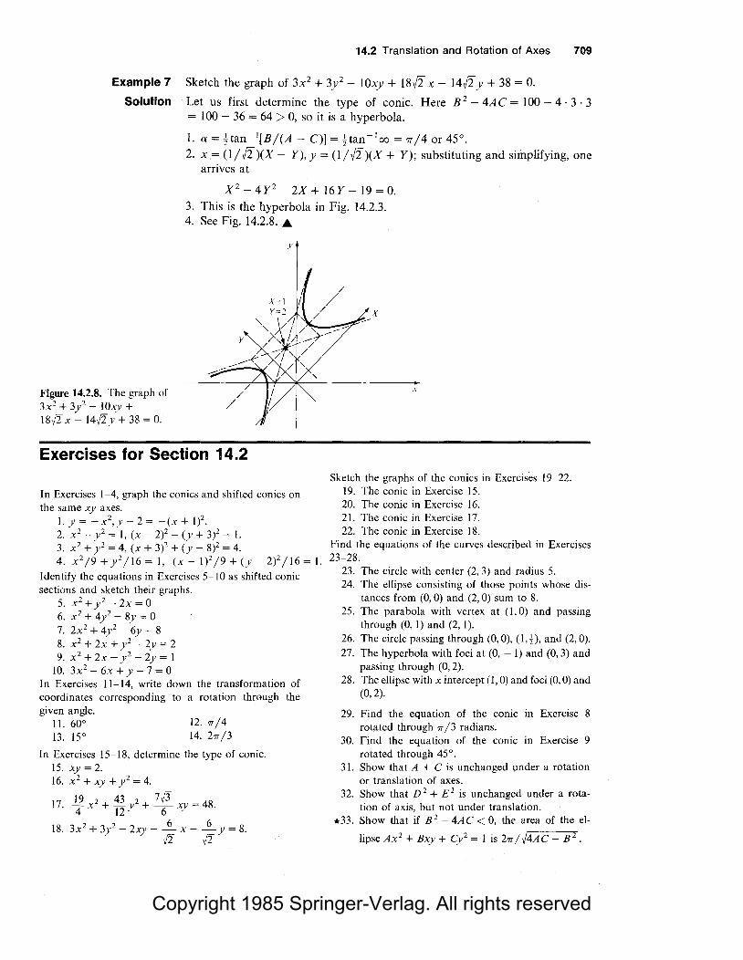
Copyright 1985 Springer-Verlag. All rights reserved
14.2 Translation and Rotation of Axes 709
Example 7 Sketch the graph of 3x2 + 3y2 - 10xy + I8v'2 x - 14v'2 y + 38 = 0.
Solution Let us first determine the type of conic. Here B 2 - 4A C = 100 - 4 . 3 . 3
= 100 - 36 = 64 > 0, so it is a hyperbola.
1. a= 1tan- 1[B/(A - C)] = 1tan- 1oo = 7r/4 or 45°. 2. x.= (I/ft)(X - Y),y = (l/ft)(X + Y); substituting and simplifying, one
arrives at
X 2 -4Y2 -2x+ 16Y-19=0.
3. This is the hyperbola in Fig. 14.2.3. 4. See Fig. 14.2.8 ...
Figure 14.2.8. The graph of 3x2 + 3y2
- lOxy + 18i/2 x - 14i/2y + 38 = 0.
Exercises for Section 14.2
)'
In Exercises 1-4, graph the conics and shifted conics on the same xy axes.
I. y = - x 2, y - 2 = -(x + 1)2
•
2. x 2 - y 2 = 1, (x - 2)2
- (y + 3)2 = I. 3. x 2 + y 2 = 4, (x + 3)2 + (y - 8)2 = 4. 4. x 2 /9+y 2 /16=1, (x-1)2 /9+(y-2)2 /!6=1.
Identify the equations in Exercises 5- JO as shifted conic sections and sketch their graphs.
5. x 2 + y 2 - 2x = 0 6. x 2 + 4y2 - Sy= 0 7. 2x2 + 4y2 - 6y = 8 8. x 2 + 2x + y 2 - 2y = 2 9. x 2 + 2x - y 2 - 2y = 1
10. 3x 2 - 6x + y - 7 = 0 In Exercises 11-14, write down the transformation of coordinates corresponding to a rotation through the given angle.
11. 60° 13. 15°
12. 'IT/4 14. 2'1T/3
In Exercises 15-18, determine the type of conic. 15. xy = 2. 16. x 2 + xy + y 2 = 4.
17. l2x2+ 43 2+ 7ff =48 4 12 Y 6 xy ·
18 , 2 6 6 . 3x" + 3y - 2xy - - x - -y = 8. V2 V2
x
Sketch the graphs of the conics in Exercises 19-22. 19. The conic in Exercise 15. 20. The conic in Exercise 16. 21. The conic in Exercise 17. 22. The conic in Exercise 18.
Find the equations of the curves described in Exercises 23-28.
23. The circle with center (2, 3) and radius 5. 24. The ellipse consisting of those points whose dis
tances from (0, 0) and (2, 0) sum to 8. 25. The parabola with vertex at (1, 0) and passing
through (0, 1) and (2, 1 ). 26. The circle passing through (0, 0), ( 1, ± ), and (2, 0). 27. The hyperbola with foci at (0, - 1) and (0, 3) and
passing through (0, 2). 28. The ellipse with x intercept (1, 0) and foci (0, 0) and
(0, 2).
29. Find the equation of the conic m Exercise 8 rotated through 'IT /3 radians.
30. Find the equation of the conic m Exercise 9 rotated through 45°.
31. Show that A + C is unchanged under a rotation or translation of axes.
32. Show that D 2 + £ 2 is unchanged under a rotation of axis, but not under translation.
*33. Show that if B 2 - 4AC < 0, the area of the el-
lipse Ax2 + Bxy + Cy2 = 1 is 2'1T /,/4AC - B 2 .

Copyright 1985 Springer-Verlag. All rights reserved
710 Chapter 14 Curves and Surfaces
14.3 Functions, Graphs, and Level Surfaces
Figure 14.3.1. Isotherms are lines of constant temperature (in degrees Celsius).
The graph of a function of two variables is a surface in space.
The daily weather map of North America shows the temperatures of various locations at a fixed time. If we let x be the longitude and y the latitude of a point, the temperature T at that point may be thought of as a function of the pair (x, y). Weather maps often contain curves through points with the same temperature. These curves, called isotherms, help us to visualize the temperature function; for instance, in Fig. 14.3.1 they help us to locate a hot spot in the southwestern U.S. and a cold spot in Canada.
Functions of two variables arise in many other contexts as well. For instance, in topography the height h of the land depends on the two coordinates that give the location. The reaction rate a of two chemicals A and B depends on their concentrations a and b. The altitude a of the sun in the sky on June 21 depends on the latitude I and the number of hours t after midnight.
Many quantities depend on more than two variables. For instance, the temperature can be regarded as a function of the time t as well as of x and y to give a function of three variables. (Try to imagine visualizing this function by watching the isotherms move and wiggle as the day progresses.) The rate of a reaction involving 10 chemicals is a function of 10 variables.
In this book we limit our attention to functions of two and three variables. Readers who have mastered this material can construct for themselves, or find in a more advanced work, 1 the generalizations of the concepts presented here to functions of four and more variables.
1 See, for example, J. Marsden and A. Tromba, Vector Calculus, Second Edition, W. H. Freeman and Co., 1980.

Copyright 1985 Springer-Verlag. All rights reserved
14.3 Functions, Graphs, and Level Surfaces 711
The mathematical development of functions of several variables begins with some definitions.
Functions of Two Variables A function of two variables is a rule which assigns a number f(x, y) to each point (x, y) of a domain in the xy plane.
Example 1 Describe the domain of f(x, y) = x/(x2 + y 2). Evaluate f(l,O) andf(l, 1).
Solution As given, this function is defined as long as x 2 + y 2 =!= 0, that is, as long as (x, y) =!= (0, 0). We have
f( l 0) = I = I and f(l 1) I .A. ' 12+02 ' = 12+12=2·
The Graph of a Function The graph of a function f(x, y) of two variables consists of all points (x,y,z) in space such that (x,y) is in the domain of the function and z = f(x,y).
Some particularly simple graphs can be drawn on the basis of our work in earlier chapters.
Example 2 Sketch the graph of (a) f(x, y) = x - y + 2 and (b) f(x, y) = 3x.
Solution (a) We recognize z = x - y + 2 (that is, x - y - z + 2 = 0) as the equation of a plane. Its normal is (I, - I, - I) and it meets the axes at ( - 2, 0, 0), (0, 2, 0), (0, 0, 2). From this information we sketch its graph in Fig. 14.3.2. (b) The graph of f(x, y) = 3x is the plane z = 3x. It contains they axis and is shown in Fig. 14.3.3 . .A.
Figure 14.3.2. The graph of z = x - y + 2 is a plane.
y
Figure 14.3.3. The graph of z = 3x.

Copyright 1985 Springer-Verlag. All rights reserved
712 Chapter 14 Curves and Surfaces
Using level curves instead of graphs makes it possible to visualize a function of two variables by a two-dimensional rather than a three-dimensional picture.
level Curves Let f be a function of two variables and let c be a constant. The set of all (x, y) in the plane such that j(x, y) = c is called a level curve off (with value c).
Isotherms are just the level curves of a temperature function, and a contour plot of a mountain consists of representative level curves of the height function.
Example 3 Sketch the level curves with values -1, 0, 1 for j(x, y) = x - y + 2.
Solution The level curve with value - l is obtained by setting j(x, y) = - 1; that is,
x - y + 2 = - 1, that is, x - y + 3 = 0,
which is a straight line in the plane (see Fig. 14.3.4). The level curve with value Y zero is the line
l t c=+l c = 0
c =-I
x
Example 4
Solution
Figure 14.3.5. The level curve ofj(x, y) with value c is obtained by finding the intersection of the graph of f with the plane z = c and moving it down to the (x, y) plane.
x - y + 2 = 0,
and the curve with value 1 is the line
x - y + 2 = 1,
Figure 14.3.4. Three level curves of the function j(x, y) = x - y + 2.
that is, x - y + 1 = 0 . .&.
How is the intersection of the plane z = c with the graph of j(x, y) related to the level curves off? Sketch.
The intersection of the plane z = c and the graph of J consists of the points ( x, y, c) in space such that j( x, y) = c. This set has the same shape as the level curve with value c, but it is moved from the xy plane up to the plane z = c. (See Fig. 14.3.5.) .&.
z Graph of f(x, y)
We turn now to functions of three variables.
Functions of Three Variables A function of three variables is a rule which assigns a numberj(x,y,z) to each point (x, y, z) of a domain in (x, y, z) space.

Copyright 1985 Springer-Verlag. All rights reserved
14.3 Functions, Graphs, and Level Surfaces 713
The graph of a function w = f ( x, y, z) of three variables would have to lie in four-dimensional space, so we cannot visualize it; but the concept of level curve has a natural extension.
Level Surfaces Let f be a function of three variables and let c be a constant. The set of all points (x, y,z) in space such thatf(x, y,z) = c is called a level surface off (with value c).
Example 5 (a) Let f(x, y,z) = x - y + z + 2. Sketch the level surfaces with values 1, 2, 3. (b) Sketch the level surface of f(x, y,z) = x 2 + y 2 + z2
- 8 with value 1.
Solution (a) In each case we set f(x, y, z) = c:
Figure 14.3.6. Three level surfaces of the function f(x, y,z) = x - y + z + 2.
Figure 14.3.7. The level surface of x 2 + y 2 + z 2
- 8 with value 1 is a sphere of radius 3.
c = 1: x - y + z + 2 = 1 (that is, x - y + z + 1 = 0),
c = 2: x - y + z + 2 = 2
c = 3: x - y + z + 2 = 3
(that is, x - y + z = 0),
(that is, x - y + z - 1 = 0).
These surfaces are parallel planes and are sketched in Fig. 14.3.6. z
x
(b) The surface x 2 + y 2 + z2 - 8 = 1 (that is, x 2 + y 2 + z 2 = 9) is the set
of points (x, y,z) whose distance from the origin is /9 = 3; it is a sphere with radius 3 and center at the origin. (See Fig. 14.3.7.) A
Plotting surfaces in space is usually more difficult than plotting curves in the plane. It is rare that plotting a few points on a surface will give us enough information to sketch the surface. Instead we often plot several curves on the surface and then interpolate between the curves. This technique, called the method of sections, is useful for plotting surfaces in space, whether they be graphs of functions of two variables or level surfaces of functions of three variables. The idea behind the method of sections is to obtain a picture of the

Copyright 1985 Springer-Verlag. All rights reserved
714 Chapter 14 Curves and Surfaces
surface in space by looking at its slices by planes parallel to one of the coordinate planes. For instance, for a graph z = f(x, y) the section z = c is illustrated in Fig. 14.3.8.
z =constant
~ I l
y
Figure 14.3.8. The section z = c of the graph
I I v----q_ Level curve in_>--
xy plane z = f(x, y). x
Example 6 Sketch the surfaces in xyz space given by (a) z = - y 2 and (b) x 2 + y 2 = 25.
Solution (a) Since x is missing, all sections x = constant look the same; they are copies of the parabola z = - y 2
• Thus we draw the parabola z = - y 2 in the yz plane and extend it parallel to the x axis as shown in Fig. 14.3.9. The surface is called a parabolic cylinder.
z
x
Figure 14.3.9. The graph z = -- y 2 is a parabolic cylinder.
y
z=-y 2 ,x=O
z
Figure 14.3.10. The graph x 2 + y 2 = 25 is a right circular cylinder.
(b) The variable z does not occur in the equation, so the surface is a cylinder parallel to the z axis. Its cross section is the plane curve x 2 + y 2 = 25, which is a circle of radius 5, so the surface is a right circular cylinder, as shown in Fig. 14.3.10 ....
Example 7 (a) Sketch the graph of f(x, y) = x 2 + y 2 (this graph is called a paraboloid of revolution). (b) Sketch the surface z = x 2 + y 2
- 4x - 6y + 13. [Hint: Complete the square.]
Solution (a) If we set z =constant, we get x 2 + y 2 = c, a circle. Taking c = 12, 22
, 32, 42
,
we get circles of radius l, 2, 3, and 4. These are placed on the planes z = 12 = 1, z = 22 = 4, z = 32 = 9, and z = 42 = 16 to give the graph shown in Fig. 14.3.11.
If we set x = 0, we obtain the parabola z = y 2; if we set y = 0, we obtain
the parabola z = x 2• The graph is symmetric about the z axis since z depends
only on r = ~ x 2 + y 2 •

Copyright 1985 Springer-Verlag. All rights reserved
14.3 Functions, Graphs, and Level Surfaces 715
(b) Completing the square, we write z = x 2 + y 2 - 4x - 6y + 13 as
z=x2 -4x+ y 2 -6y +13 = x 2
- 4x + 4 + y 2 - 6y + 9 + 13 - 13
= (x - 2)2 + (y - 3)2.
The level surface for value c is thus the circle (x - 2)2 + (y - 3)2 = c with center (2, 3) and radius fC. Comparing this result with (a) we find that the surface is again a paraboloid of revolution, with its axis shifted to the line (x, y) = (2, 3). (See Fig. 14.3.12.) .&.
2
16 x2 + y2 = 42
x2 + y2 = 32
y
x
z
x I {x= 2 1--1 y = 3
Figure 14.3.12. The graph
y
Figure 14.3.11. The sections of the graph z = x 2 + y 2 by planes z = c are circles.
z = x 2 + y 2 - 4x - 6y + 13 is a shifted paraboloid of revolution.
Plotting Surfaces: Methods of Sections l. Note any symmetries of the graph. 2. See if any variables x, y, or z are missing from the equation. If so, the
surface is a "cylinder" parallel to the axis of the missing variable, and its cross section is the curve in the other variables (see Example 6).
3. If the surface is a graph z = j(x, y), find the level curves f(x, y) = c for various convenient values of c and draw these curves on the planes z = c. Smoothly join these curves with a surface in space. Draw the curves obtained by setting x = 0 and y = 0 or other convenient values to help clarify the picture.
4. If the surface has the form F(x, y, z) = c, then either: (a) Solve for one of the variables in terms of the other two and use
step 2 if it is convenient to do so. (b) Set x equal to various constant values to obtain curves in y and z;
draw these curves on the corresponding x =constant planes. Repeat with y = constant or z = constant or both. Fill in the curves obtained with a surface.

Copyright 1985 Springer-Verlag. All rights reserved
716 Chapter 14 Curves and Surfaces
'l
0
~s i
-2
Figure 14.3.13. The graph of z = x 2 + y 2 drawn by computer in two ways.
In the next section, we will use our knowledge of conic sections to plot the graphs of more complicated quadratic functions.
The computer can help us graph surfaces that may be tedious or impossible to plot by hand. The computer draws the graph either by drawing sections perpendicular to the x and y axes or by sections perpendicular to the z axis-that is, level curves lifted to the graph. When this is done for the function z = x 2 + y 2 (Example 7), Figs. 14.3.13(a) and 14.3.13(b) result. (The pointed tips appear because a rectangular domain has been chosen for the function.)2
'J
I 0 "'ll1s 1
-2
The computer-generated graph in Fig. 14.3.14 shows the function
z = (x2 + 3y2)el-(x2+y2l.
Fig. 14.3.15 shows the level curves of this function in the xy plane, viewed first from an angle and then from above. Study these pictures to help develop your powers of three-dimensional visualization; attempt to reconstruct the graph in your mind by looking at the level curves.
2 The authors are indebted to Jerry Kazdan for preparing most of the computer-generated graphs in this book.

Copyright 1985 Springer-Verlag. All rights reserved
(a)
(b)
Figure 14.3.14. Computergenerated graphs of z = (x2 + 3y2)el-(x'+y').
Figure 14.3.15. Level curves for the function z = (x 2 + 3y2)e1-(x2 +y'J.
(a)
(b)
14.3 Functions, Graphs, and Level Surfaces 717
l.5
t.o
·S

Copyright 1985 Springer-Verlag. All rights reserved
718 Chapter 14 Curves and Surfaces
Exercises for Section 14.3 In Exercises 1-8, describe the domain of each of the given functions and evaluate the function at the indicated points.
1. j(x, y) = 2'.; (1,0), (1, 1). x
- x+ y. 2. f(x, y) - -- , (I, -1), (1, 0.9). x-y
- x+ y . 3. j(x, y) - , (1, 1), (-1, 1). x2 + y2 - 1
_ 2xy . 4. j(x, y)- -- , (1, 1), (-1, 1).
x2 + y2
_ 2x + y- z . 5. f(x, y, z) - 2 , (1, 1, 1), (0, 0, 2).
x 2 + y + z2 - 1
6. f(x, y, z) = z ; (1, 0.5, 1), (0.1, 0.5, 1). x 2
- 4y2 - 1
_ 2x - siny. 7.f(x,y)-
1 ,(0,?T/4),('1T/4,'1T). + cosx
ex - eY 8. f(x, y) =
1 . ; (0, l); ('1T /4, -1). + smx
Sketch the graphs of the functions in Exercises 9-12. 9. f(x, y) = 1 - x - y 10. f(x, y) = -1 - x - y
11. z = x - y 12. z = x + 2 Sketch the level curves for the indicated functions and values in Exercises 13-18.
13. fin Exercise 9, values 1, -1. 14. fin Exercise 10, values 1, - 1. 15. fin Exercise 3, values -2, -1, 1, 2 and describe
the level curve for the general value. 16. f in Exercise 4, values - 2, - 1, 1, 2 and describe
the level curve for the general value. 17. f in Exercise 2, values - 2, - 1, 1, 2 and describe
the level curve for the general value. 18. j(x, J) = r I/(x
2+Y
2), value 1/ e.
Sketch the level surfaces in Exercises 19-22. 19. x + y - 2z = 8 20. 3x - 2y - z = 4 21. x 2 + y 2 + z 2 = 4 22. x 2 + y 2
- z = 4 Draw the level curves f(x, y) = c-first in the xy plane and then lifted to the graph in space-for the functions and values in Exercises 23-26.
23. f(x, y) = x 2 + 2y2; c = 0, 1,2. 24. f(x, y) = x 2
- y 2; c = - 1, 0, 1.
25. f(x,y) = x- y 2; c = -2,0,2. 26. f(x, y) = y - x 2
; c = - 1, 0, 1. Sketch the surface in space defined by each of the equations in Exercises 27-40.
27. z = x 2 + 2 29. z 2 + x 2 = 4 31. z = (x - 1)2 + y 2
33. z = x 2 + y 2 L 2x + 8.
28. z = IYI 30. x 2 + y = 2 32. x = - 8z 2 + z
34. z = 3x 2 + 3y2 - 6x + 12y + 15.
35. z = .Jx2 + y 2
36. z = max(lxl, lyl). [Note: max(lxl, lyl) is the maximum of lxl and IYl·l
37. z = sinx (the "washboard").
38. z = 1/(1 + y 2).
39. 4x2 + y 2 + 9z2 = 1.
40. x 2 + 4y 2 + 16z2 = 1. 41. Let j(x, y) = e- 1/<x
2+Y
2l; j(O, 0) = 0.
(a) Sketch the level curve j(x, y) = c for c = 0.001, c = 0.01, c = 0.5, and c = 0.9.
(b) What happens if c is less than zero or greater than 1?
(c) Sketch the cross section of the graph in the vertical plane y = 0 (that is, the intersection of the graph with the xz plane).
(d) Argue that this cross section looks the same in any vertical plane through the origin.
(e) Describe the graph in words and sketch it. trrj42. The formula
2x z=-------(y- y-1)2 + (2x)2
appears in the study of steady state motions of a mechanical system with viscous damping subjected to a harmonic external force. The average power input by the external force is proportional to the variable z (with proportionality constant k > 0). The variable y is the ratio of input frequency to natural frequency. The variable x measures the viscous damping constant. (a) Plot z versus y for x = 0.2, 0.5, 2.0 on the
same axes. Use the range of values 0 < y <: 2.0.
(b) The average power input is a maximum when y = 1, that is, when the input and natural frequencies are the same. Verify this both graphically and algebraically.
43. The potential difference E between electrolyte solutions separated by a membrane is given by
E = RT x - y lnz. F x + y
(The symbols R, T, F are the universal gas constant, absolute temperature, and Faraday unit, respectively-these are constants. The symbols x and y are the mobilities of Na+ and Cl - respectively. The symbol z is cif c2 , where c1 and c2 are the mean salt (NaCl) concentrations on each side of the membrane.) Assume hereafter that RT/ F = 25. (a) Write the level surface E = - 12 in the form
z = f(x, y). (b) In practice, y = 3x /2. Plot E versus z in this
case. *44. Describe the behavior, as c varies, of the level
curve f(x, y) = c for each of these functions: (a) f(x, y) = x 2 + y 2 + l; (b) f(x,y)= l -x2 - y 2
;
(c) j(x, y) = x 2 + xy; (d) j(x, y) = x 3 - x.

Copyright 1985 Springer-Verlag. All rights reserved
14.4 Quadric Surfaces 719
14.4 Quadric Surfaces Quadric surfaces are defined by quadratic equations in x, y, and z.
The methods of Section 14.3, together with our knowledge of conics, enable us to graph a number of interesting surfaces defined by quadratic equations.
Example 1 Sketch the graph of
z = j(x, y) = x 2 - y 2 (a hyperbolic paraboloid).
Solution To visualize this surface, we first draw the level curves x 2 - y 2 = c for c = 0, ± l, ±4. For c = 0 we have y 2 = x 2 (that is, y = ± x), so this level set consists of two straight lines through the origin. For c = 1 the level curve is x 2
- y 2 = 1, which is a hyperbola that passes vertically through the x axis at the points ( ± 1, 0) (see Fig. 14.4.1 ). Similarly, for c = 4 the level curve is x 2
/ 4 - y 2 / 4 = 1, the hyperbola passing vertically through the x axis at
( ± 2, 0). For c = - 1 we obtain the hyperbola x 2 - y 2 = - 1 passing horizon
tally through the y axis at (0, ± 1 ), and for c = - 4 the hyperbola through (0, ± 2) is obtained. These level curves are shown in Fig. 14.4.1. To aid us in visualizing the graph off, we will also compute two sections. First, set x = 0 to obtain z = - y 2
, a parabola opening downward. Second, setting y = 0 gives the parabola z = x 2 opening upward.
Figure 14.4.1. Some level curves ofj(x) = x 2 - y 2.
y
x
x2 _ y2 = -22
The graph may now be visualized if we lift the level curves to the appropriate heights and smooth out the resulting surface. The placement of the lifted curves is aided by the use of the parabolic sections. This procedure generates the saddle-shaped surface indicated in Fig. 14.4.2. The graph is unchanged under reflection in the yz plane and in the xz plane. When accurately plotted by a computer, this graph has the appearance of Fig. 14.4.3; the level curves are shown in Fig. 14.4.4. (The graph has been rotated by 90° about the z axis.) .Ai.

Copyright 1985 Springer-Verlag. All rights reserved
-1
-2
(a)
720 Chapter 14 Curves and Surfaces
Figure 14.4.2. The graph z = x 2
- y 2 is a hyperbolic paraboloid, or "saddle."
Figure 14.4.3. Computergenerated graph of z = x2 - y2.
Figure 14.4.4. Level curves of z = x 2 - y 2 drawn by computer.
z
x2 -y2 = -(12)
y
-1
-2
_, -, -s
(b)

Copyright 1985 Springer-Verlag. All rights reserved
Figure 14.4.5. Graph of the monkey saddle: z = x 3 - 3xy2 •
Figure 14.4.6. Level curves for the monkey saddle.
14.4 Quadric Surfaces 721

Copyright 1985 Springer-Verlag. All rights reserved
722 Chapter 14 Curves and Surfaces
The origin is called a saddle point for the function z = x 2 - y 2 because of the
appearance of the graph. We will return to the study of saddle points in Chapter 16, but it is worth noting another kind of saddle here. Figure 14.4.5 on the preceding page shows the graph of z = x 3
- 3xy2, again plotted by a
computer using sections and level curves. The origin now is called a monkey saddle, since there are two places for the legs and one for the tail. Figure 14.4.6 shows the contour lines in the plane. Figure 14.4.7 shows the four-legged or dog saddle: z = 4xy - 4xy 3
•
Figure 14.4.7. The dog saddle: z = 4x3y - 4xy3
•

Copyright 1985 Springer-Verlag. All rights reserved
14.4 Quadric Surfaces 723
A quadric surface is a three-dimensional figure defined by a quadratic equation in three variables:
ax2 + by2 + cz 2 + dxy + exz + fyz + gx + hy + kz + m = 0.
The quadric surfaces are the three-dimensional versions of the conic sections, studied in Section 14.1, which were defined by quadratic equations in two variables.
Example 2 Particular conic sections can degenerate to points or lines. Similarly, some quadric surfaces can degenerate to points, lines, or planes. Match the sample equations to the appropriate descriptions.
(a) x 2 + 3y2 + z 2 = 0 (b) z 2 =0 (c) x 2 + y 2 = 0 ( d) x 2 + y 2 + z2 + 1 = 0 (e) x 2
- y 2 = 0
(1) No points at all (2) A single point (3) A line (4) One plane (5) Two planes
Solution Equation (a) matches (2) since only (0, 0, 0) satisfies the equation; (b) matches (4) since this is the plane z = O; (c) matches (3) since this is the z axis, where x = 0 and y = O; (d) matches (1) since a non-negative number added to 1 can never be zero; (e) matches (5) since the equation x 2
- y 2 = 0 is equivalent to the two equations x + y = 0 or x - y = 0, which define two planes . .A.
If one variable is missing from an equation, we only have to find a curve in one plane and then extend it parallel to the axis of the missing variable. This procedure produces a generalized cylinder, either elliptic, parabolic, or hyperbolic .
. Example 3 Sketch the surface z = y 2 + 1.
Solution The intersection of this surface with a plane x = constant is a parabola of the form z = y 2 + 1. The surface, a parabolic cylinder, is sketched in Fig. 14.4.8. (See also Example 6, Section 14.3) . .A.
Figure 14.4.8. The surface z = y 2 + I is a parabolic cylinder.
z
y

Copyright 1985 Springer-Verlag. All rights reserved
724 Chapter 14 Curves and Surfaces
Example 4 The surface defined by an equation of the form x 1 / a1 + y 1
/ b1 - z 1
/ c1 = - 1 is called a hyperboloid of two sheets. Sketch the surface x 1 + 4y1
- z 1 = - 4.
Solution The section by the plane z = c has the equation x 1 + 4y1 = c1 - 4. This is an
ellipse when lei > 2, a point when c = ± 2, and is empty when lcl < 2. The section with the xz plane is the hyperbola x 1
- z1 = - 4, and the section with the yz plane is the hyperbola 4y2 - z 1 = - 4. The surface is symmetric with respect to each of the coordinate planes. A sketch is given in Fig. 14.4.9 . ..&.
Figure 14.4.9. The surface x 2 + 4y2 - z 2 = - 4 is a hyperboloid of two sheets (shown with some of its sections by planes of the form z = constant).
z
y
Example 5 The surface defined by an equation of the form x 1 / a1 + y 1
/ b1 + z1 / c1 = I is
called an ellipsoid. Sketch the surface x 2 /9 + y 2 /16 + z 2 = 1.
Solution First, let z be constant. Then we get x 2 /9 + y 1 /16 = 1 - z1. This is an ellipse
centered at the origin if - 1 < z < 1. If z = 1, we just get a point x = 0, y = 0. Likewise, (0, 0, - I) is on the surface. If lzl > 1 there are no (x, y) satisfying the equation.
Figure 14.4.10. The surface (x 2 /9) + (y 2 /16) + z2 = l is an ellipsoid.
Setting x =constant or y =constant, we also get ellipses. We must have lxl < 3 and, likewise, IYI < 4. The surface, shaped like a stepped-on football, is easiest to draw if the intersections with the three coordinate planes are drawn first. (See Fig. 14.4.10.) ..&.
z
" y (0,4,0)

Copyright 1985 Springer-Verlag. All rights reserved
14.4 Quadric Surfaces 725
Example 6 The surface defined by an equation of the form x 2 / a2 + y 2
/ b2 - z 2
/ c2 = I is called a hyperboloid of one sheet. Sketch the surface x 2 + y 2
- z 2 = 4.
Solution If z is a constant, then x 2 + y 2 = 4 + z 2 is a circle. Thus, in any plane parallel to the xy plane, we get a circle. Our job of drawing the surface is simplified if we note right away that the surface is rotationally invariant about the z axis (since z depends only on r 2 = x 2 + y 2). Thus we can draw the curve traced by the surface in the yz plane (or xz plane) and revolve it about the z axis. Setting x ~ 0, we get y 2
- z 2 = 4, a hyperbola. Hence we get the surface shown in Fig. 14.4.11, a one-sheeted hyperboloid. Since this surface is symmetric about the z axis, it is also called a hyperboloid of revolution. A
Figure 14.4.11. The surface x 2 + y 2 - z 2 = 4 is a one-sheeted hyperboloid of revolution.
Figure 14.4.12. One can make a hyperboloid with a wire frame and string.
z
y
The hyperboloid of one sheet has the property that it is ruled: that is, the surface is composed of straight lines (see Review Exercise 76). It is therefore easy to make with string models and is useful in architecture. (See Fig. 14.4.12.)
Example 7 Consider the equation x 2 + y 2 - z2 = 0.
(a) What are the horizontal cross sections for z = ± 1, ± 2, ± 3? (b) What are the vertical cross sections for x = 0 or y = O? (Sketch and
describe.) (c) Show that this surface is a cone by showing that any straight line through
the origin making a 45° angle with the z axis lies in the surface. ( d) Sketch this surface.

Copyright 1985 Springer-Verlag. All rights reserved
726 Chapter 14 Curves and Surfaces
Solution (a) Rewriting the equation as x2 + y 2 = z
2 shows that the horizontal cross sections are circles centered around the z axis with radius lzl. Therefore, for z = ± 1, ± 2, and ± 3, the cross sections are circles of radius l, 2, and 3.
Figure 14.4.13. The cone x2 + y2 - z2 = 0.
(b) When x = 0, the equation is y 2 - z2 = 0 or y 2 = z2 or y = ± z, whose graph is two straight lines. When y = 0, the equation is x 2
- z 2 = 0 or x = ± z, again giving two straight lines.
(c) Any point on a straight line through the origin making a 45° angle with
the z axis satisfies lzl/~x2 + y 2 + z 2 = cos45° = 1//2. Squaring gives 1/2=z2
/(x2 +y2 +z2
), or x2 +y2 +z2 =2z2
, or x2 +y2 -z2 =0,
which is the original equation. (d) Draw a line as described in part (c) and rotate it around the z axis (see
Figure 14.4.13). A
z
For x = 0 For y = 0
z z
y
y y
x
y = ±z
We now discuss how the conic sections, as introduced in the first section of this chapter, can actually be obtained by slicing a cone.
Example 8 Show that the intersection of the cone x2 + y 2 = z
2 and the plane y = 1 is a hyperbola (see Figure 14.4.14).
Figure 14.4.14. The intersection of this vertical plane and the cone is a hyperbola. Hyperbola
y

Copyright 1985 Springer-Verlag. All rights reserved
14.4 Quadric Surfaces 727
Solution The intersection of these two surfaces consists of all points (x,y,z) such that x 2 + y 2 = z 2 and y = 1. We can use x and z as coordinates to describe points in the plane. Thus, eliminating y, we get x 2 + 1 = z 2 or z 2
- x 2 = 1. From Section 14.1, we recognize this as a hyperbola with foci at x = 0, z = ±.ff in the plane y = 1, with the branches opening vertically as in the figure . .A
Example 9 Show that the intersection of the cone x 2 + y 2 = z 2 and the plane z = y - 1 is a parabola (see Figure 14.4.15).
Solution We introduce rectangular coordinates on the plane as follows. A normal vector to the plane is n = (0, 1, - 1), and so a vector w =(a, b, c) is parallel to the plane if 0 = n · w = b - c. Two such vectors that are orthogonal and of unit length are
(\ Figure 14.4.15. The intersection of the plane tilted at 45° and the cone is a parabola.
u = i and v = - 1- (j + k) . .ff
Pick a point on the plane, say P0 = (0,0, -1), and write points P = (x, y,z) in the plane in terms of coordinates (~, 71) by writing --PoP = ~u + 71v
(see Fig. 14.4.16). In terms of (x, y,z), this reads T/
x = ~. y =.ff ' and z = _!]_ - 1. .ff
Figure 14.4.16. Coordinates (~, 11) in the plane z = y - I.
Substitution into x 2 + y 2 = z 2 gives
712 ( T/ )2 712 r:; e + 2 = .ff - 1 = 2 - v211 + 1,
or
e=-../211+1,
or
T/ = - _l_ ~2 + _l_ . .ff .ff
x
z
This, indeed, is a parabola opening downwards in the ~T/ plane . .A
z = y-1
y
Other sections of the cone can be analyzed in a similar way, and one can prove that a conic will always result (see Exercise 27).
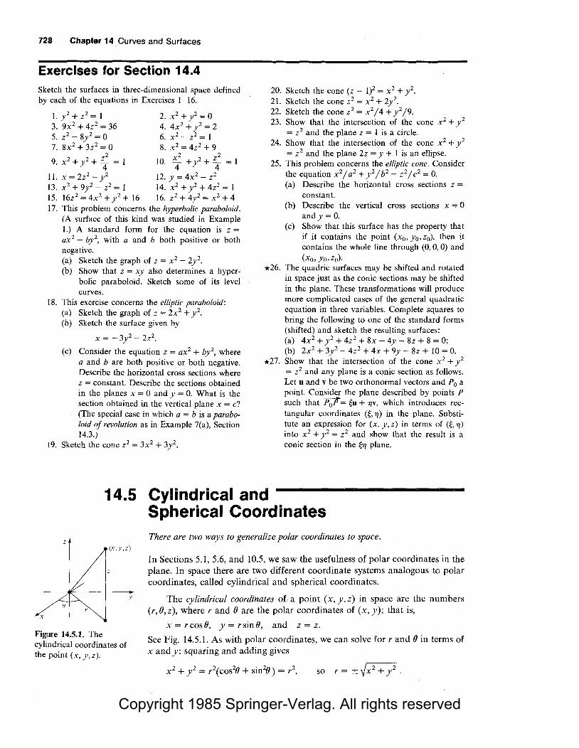
Copyright 1985 Springer-Verlag. All rights reserved
728 Chapter 14. Curves and Surfaces
Exercises for Section 14.4 Sketch the surfaces in three-dimensional space defined by each of the equations in Exercises l -16.
20. Sketch the cone (z - 1)2 = x 2 + y 2•
21. Sketch the cone z 2 = x 2 + 2y2•
x
I. y 2 + z2 = l 2. x 2 + y 2 = 0 3. 9x2 + 4z2 = 36 4. 4x2 + y 2 = 2 5. z2 - 8y2 = 0 6. x 2 - z2 = I 7. 8x2 + 3z2 = 0 8. x 2 = 4z2 + 9
z2 x2 z2 9. x2 + y2 + 4 = l IO. 4 + y2 + 4 = l
11. x = 2z2 - y 2 12. y = 4x2 - z2
13. x 2 + 9y2 - z2 = 1 14. x2 + y 2 + 4z2 = 1 15. 16z2 = 4x2 + y 2 + 16 16. z2 + 4y2 = x 2 + 4 17. This problem concerns the hyperbolic paraboloid.
(A surface of this kind was studied in Example 1.) A standard form for the equation is z = ax2
- by2, with a and b both positive or both
negative. (a) Sketch the graph of z = x 2
- 2y2.
(b) Show that z = xy also determines a hyperbolic paraboloid. Sketch some of its level curves.
18. This exercise concerns the elliptic paraboloid: (a) Sketch the graph of z = 2x2 + y 2
.
(b) Sketch the surface given by
x = -3y2 - 2z2.
(c) Consider the equation z = ax2 + by2, where a and b are both positive or both negative. Describe the horizontal cross sections where z =constant. Describe the sections obtained in the planes x = 0 and y = 0. What is the section obtained in the vertical plane x = c? (The special case in which a = b is a paraboloid of revolution as in Example 7(a), Section 14.3.)
19. Sketch the cone z2 = 3x2 + 3y2•
22. Sketch the cone z2 = x 2 / 4 + y 2 /9.
23. Show that the intersection of the cone x 2 + y 2
= z2 and the plane z = 1 is a circle. 24. Show that the intersection of the cone x 2 + y 2
= z 2 and the plane 2z = y + 1 is an ellipse. 25. This problem concerns the elliptic cone. Consider
the equation x 2 / a2 + y 2 / b2 - z2/ c2 = 0.
(a) Describe the horizontal cross sections z =
constant. (b) Describe the vertical cross sections x = 0
andy = 0. (c) Show that this surface has the property that
if it contains the point (x0 , y 0 , z0), then it contains the whole line through (0, 0, 0) and (xo, Yo, zo).
*26. The quadric surfaces may be shifted and rotated in space just as the conic sections may be shifted in the plane. These transformations will produce more complicated cases of the general quadratic equation in three variables. Complete squares to bring the following to one of the standard forms (shifted) and sketch the resulting surfaces: (a) 4x2 + y 2 + 4z2 + 8x - 4y - 8z + 8 = O; (b) 2x2 + 3y2 - 4z2 + 4x + 9y - 8z + 10 = 0.
*27. Show that the intersection of the cone x 2 + y 2
= z2 and any plane is a conic section as follows. Let u and v be two orthonormal vectors and P0 a point. Consider the plane described by points P such that P0P = ~u + 1JV, which introduces rectangular coordinates (~, 11) in the plane. Substitute an expression for ( x, y, z) in terms of ( ~, 1/)
into x 2 + y 2 = z2 and show that the result is a conic section in the ~1/ plane.
14.5 Cylindrical and Spherical Coordinates
(x,y,z)
y
There are two ways to generalize polar coordinates to space.
In Sections 5.1, 5.6, and 10.5, we saw the usefulness of polar coordinates in the plane. In space there are two different coordinate systems analogous to polar coordinates, called cylindrical and spherical coordinates.
The cylindrical coordinates of. a point (x, y, z) in space are the numbers (r, (), z), where r and () are the polar coordinates of (x, y); that is,
x = rcosB, y = rsinB, and z = z. Figure 14.5.1. The cylindrical coordinates of the point (x, y, z).
See Fig. 14.5.1. As with polar coordinates, we can solve for r and () in terms of x and y: squaring and adding gives
so r = ± ~x2 + y 2 .

Copyright 1985 Springer-Verlag. All rights reserved
14.5 Cylindrical and Spherical Coordinates 729
Dividing gives
1_ = sin8 = tan8. x cos8
As in polar coordinates, it is sometimes convenient to allow negative r; thus (r, 8) and ( - r, 8 + 'lT) represent the same point. Also, we recall that (r, 8) and (r, 8+ 2'1T) represent the same point. Sometimes we specify r > 0 (with r = 0 corresponding to the z-axis) and a definite range for 8. If we choose 8 between 'lT and - 'lT and choose tan - 1u between - 'lT /2 and 'lT /2, then the solution of y/x = tan8 is 8 = tan- 1(y/x) if x > 0, and 8 = tan- 1(y/x) + 'lT if x < 0 (8 = 'lT /2 if x = 0 and y > 0, and 8 = - 'lT /2 if x = 0 and y < 0).
Cylindrical Coordinates If the cartesian coordinates of a point in space are (x, y,z), then the cylindrical coordinates of the point are (r, 8, z), where
x = rcos8, y = rsin8, z = z;
or, if we chooser> 0 and - 'lT < 8 < 'lT,
r = -/x2 + y2 ,
if x ;;. 0,
if x < 0.
Example 1 (a) Find the cylindrical coordinates of (6, 6, 8). Plot. (b) If a point has cylindrical coordinates (3, - 'lT / 6, - 4), what are its cartesian
coordinates? Plot. ( c) Let a point have cartesian coordinates (2, - 3, 6). Find its cylindrical
coordinates and plot. (d) Let a point have cylindrical coordinates (2,3'lT/4, 1). Find its cartesian
coordinates and plot.
Solution (a) Here r =V62 + 62 = 6/i and 8 = tan- 1(V = tan- 1(1) = 'lT/4. Thus the cylindrical coordinates are (6/i, 'lT / 4, 8). See Fig. 14.5.2(a).
Figure 14.S.2. Comparing the cylindrical and cartesian coordinates of two points.
(b) x=rcos8=3cos(-'lT/6)=3f3/2, and y=rsin8=3sin(-'lT/6)= - 3 /2. Thus the cartesian coordinates are (3{3 /2, - 3 /2, -4). See Fig. 14.5.2(b).
(c) r=~r-x-2 +_y_2 =J22 +(-3)2 =fl3; 8=tan- 1(-})~-0.983~ -56.31°;z = 6. See Fig. 14.5.3(a).
x
7f
4
(a)
(6, 6, 8)
8
y
z
y
7f
-4 6
x (3VJ/2, - 3/2, -4)
(b)

Copyright 1985 Springer-Verlag. All rights reserved
730 Chapter 14 Curves and Surfaces
z
6
y y
x
Figure 14.5.3. Two points in cylindrical coordinates.
x
(a) (b)
(d) x=rcos0=2cos(3?T/4)=2·(-/2/2)= -/2;
y = rsinO = 2sin(3?T/4) = 2 ·(If /2) =If; z =I.
See Fig. 14.5.3(b) . .A
Many surfaces are easier to describe in cylindrical than in cartesian coordinates, just as many curves are easier to work with using polar rather than cartesian coordinates.
Example 2 Plot the two surfaces described in cylindrical coordinates by (a) r = 3 and (b) r = cos20.
Solution (a) Note that r is the distance from the given point to the z axis. Therefore the points with r = 3 lie on a cylinder of radius 3 centered on the z axis. See Fig. 14.5.4. (b) The curve r = cos20 in the xy plane is a four-petaled rose (see Example 1, Section 5.6). Thus in cylindrical coordinates we obtain a vertical cylinder with the four-leafed rose as a base, as shown in Fig. 14.5.5 . ..&.
t/ l .· /
z
I I ..
-----*'· /. / l
."' I /; ! / 9111 f. x .• , I
I Figure 14.5.4. The cylinder has a very simple equation in cylindrical coordinates.
Figure 14.5.5. The surface r =cos 20 is a cylinder with a four-petaled rose as its base. x
Example 3 Describe the geometric meaning of replacing (r, 0, z) by (r, () + ?T, - z).
y
Solution Increasing 0 by '1T is a rotation through 180° about the z axis. Switching z to - z reflects in the xy plane (see Fig. 14.5.6). Combining the two operations results in reflection through the origin . ..&.
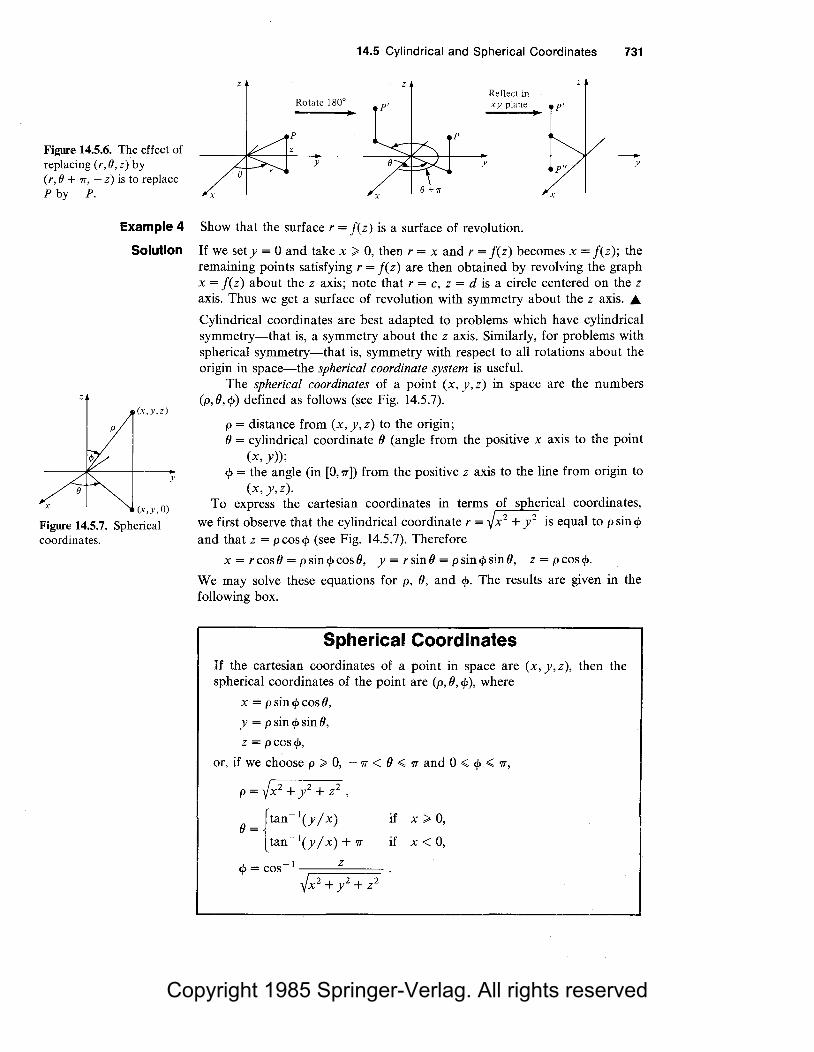
Copyright 1985 Springer-Verlag. All rights reserved
Figure 14.5.6. The effect of replacing (r,B,z) by (r,B +'TT, -z) is to replace P by -P.
Example 4
Solution
z (x,y,z)
p
x (x,y,0)
Figure 14.5.7. Spherical coordinates.
y
z
Rotate 180°
p
y
x
14.5 Cylindrical and Spherical Coordinates 731
z
p
y
e +" x
Reflect in xy plane
x
P'
z
y
Show that the surfacer= j(z) is a surface of revolution.
If we set y = 0 and take x ;;;. 0, then r = x and r = j(z) becomes x = j(z); the remaining points satisfying r = j(z) are then obtained by revolving the graph x = j(z) about the z axis; note that r = c, z = dis a circle centered on the z axis. Thus we get a surface of revolution with symmetry about the z axis. JJ,,.
Cylindrical coordinates are best adapted to problems which have cylindrical symmetry-that is, a symmetry about the z axis. Similarly, for problems with spherical symmetry-that is, symmetry with respect to all rotations about the origin in space-the spherical coordinate system is useful.
The spherical coordinates of a point (x, y,z) in space are the numbers (p, 0, cf>) defined as follows (see Fig. 14.5.7).
p =distance from (x, y,z) to the origin; 0 =cylindrical coordinate 0 (angle from the positive x axis to the point
(x, y)); cf> = the angle (in [O, w]) from the positive z axis to the line from origin to
(x, y,z). To express the cartesian coordinates in terms-/. of spherical coordinates,
we first observe that the cylindrical coordinate r = x 2 + y 2 is equal to p sin cf> and that z = pcoscp (see Fig. 14.5.7). Therefore
x = rcosO = psincpcosO, y = rsinO = psincpsinO, z = pcoscp.
We may solve these equations for p, 0, and cf>. The results are given in the following box.
Spherical Coordinates If the cartesian coordinates of a point in space are (x, y,z), then the spherical coordinates of the point are (p, 0, cf>), where
x = psincpcosO,
y = p sincp sin 0,
z = pcoscp,
or, if we choose p;;;. 0, - w < 0 < wand 0 <cf>< w,
p = -J.x2 + y2 + z2 ,
{
tan- 1(y / x)
O = tan- 1(y/x) + w
cf>=cos- 1 z
-J.x2 + y2 + z2
if x;;;. 0,
if x < 0,

Copyright 1985 Springer-Verlag. All rights reserved
732 Chapter 14 Curves and Surfaces
Notice that the spherical coordinates 0 and cf> are similar to the geographic coordinates of longitude and latitude if we take the earth's axis to be the z
axis. There are differences, though: the geographical longitude is IO I and is called east or west longitude according to whether 0 is positive or negative; the geographical latitude is 1'7T /2 - <t>I and is called north or south latitude according to whether '7T /2 - cf> is positive or negative.
Example 5 (a) Find the spherical coordinates of (1, -1, 1) and plot.
Figure 14.5.8. Finding the spherical coordinates of the point (1, -1, 1) and the cartesian coordinates of (3,?T/6,?T/4).
(b) Find the cartesian coordinates of (3, '7T / 6, '7T / 4) and plot. ( c) Let a point have cartesian coordinates (2, - 3, 6). Find its spherical coordi
nates and plot. (d) Let a point have spherical coordinates (1, -'7T/2,'7T/4). Find its cartesian
coordinates and plot.
0 -1(Y) -1(-l) '7T =tan x =tan -1- =- 4 ,
cf>= cos- 1( ! ) = cos- 1
( ~) ~0.955~54.74°.
See Fig. 14.5.8(a).
z z
(I, -1, I) p=3
y y
e = -2k x x
(a) (b)
(b) . 0 . ( '7T ) ( '7T ) ( 1 ) ff 3[3 x = p sm cf> cos = 3 sm 4 cos 6 = 3 fi T = 2 fi ,
y = psin<f>sinO = 3sin( *)sin(~)= 3( fi )( t) = 2~ ,
z = p cos cf> = 3 cos( * ) = 3f .
See Fig. 14.5.8(b).
(c) p = -Jx2 + y2 + z2 = J22 + (-3)2 + 62 = /49 = 7,
0 = tan - 1 ( ~ ) = tan -- 1
( ~ 3 ) ~ - 0.983 ~ - 56.31 °
cf>= cos- 1( *) = cos- 1
( ~) ~0.541 ~31.0°.
See Fig. 14.5.9(a) (the point is the same as in Example l(d)).

Copyright 1985 Springer-Verlag. All rights reserved
Figure 14.5.9. Two points in spherical coordinates.
z
7
31°
y
x
(a)
14.5 Cylindrical and Spherical Coordinates 733
x
z
1T
4
(b)
y
(d) x = psincpcosO = 1 sin( i )cos( -2w) = ( ~ ) · 0 = 0,
y = psincpsinO = 1 sin( i )sin( -2 w) = ( ~ )(-1) = - ~ ,
z = p cos</> = 1 cos( i ) = ~ .
See Fig. 14.5.9(b ) . ..t.
Example 6 Find the equation in spherical coordinates of x 2 + y 2 - z2 = 4 (a hyperboloid of revolution).
Solution To take advantage of the relationship x 2 + y 2 + z2 = p2, write
x2 + y2 - z2 = (x2 + y2 + z2) - 2z2 = p2 - 2p2cos2cp,
since z-= pcoscp. Also, we can note that
p2 - 2p2cos2cp = p2( 1 - 2 COS2cp) = - p2cos 2cp.
Thus the surface is
p2cos 2cp + 4 = 0 . ..t.
Example 7 (a) Describe the surface given in spherical coordinates by p = 3. (b) Describe the geometric meaning of replacing (p,O,cp) by (p,O + w,cp).
Solution (a) In spherical coordinates, p is the distance from the point (x, y,z) to the origin. Thus p = 3 consists of all points a distance 3 from the origin-that is, a sphere of radius 3 centered at the origin. (b) Increasing 0 by w has the effect of rotating about the z axis through an angle of 180° . ..t.
Example 8 Show that the surface p = f ( </>) is a surface of revolution.
Solution The equation p = f(</>) does not involve 0 and hence is independent of rotations about the z axis; thus it is a surface of revolution. If we set y = 0, then p=Vx2+z2 and cp=cos- 1(z/Vx2+z2 ). Thus the surface p=f(</>) is obtained by revolving the curve in the xz plane given by
)x2+z2 =i{cos- 1( z )), \ )x2 + z2
about the z axis . .A

Copyright 1985 Springer-Verlag. All rights reserved
734 Chapter 14 Curves and Surfaces
Exercises for Section 14.5 In Exercises 1-6, convert from cartesian to cylindrical coordinates and plot:
1. (1, -1, 0) 3. (3, -2, 1) 5. (6, 0, -2)
2. (y'2,l,l) 4. (0, 6, -2) 6. ( - 1, 1, 1)
In Exercises 7-12, convert from cylindrical to cartesian coordinates and plot.
7. (1, 'IT /2, 0) 9. (-1,'IT/6,4)
11. co, 'IT/ 18, 6)
8. (3, 45°, 8) 10. (2, 0, 1) 12. c2, - 'IT/ 4, 3)
13. Sketch the surface described in cylindrical coordinates by r = 1 + 2 cos 0.
14. Sketch the surface given in cylindrical coordinates by r = 1 + cosO.
In Exercises 15-18, describe the geometric meaning of the stated replacement.
15. (r,O,z) by (r,O, -z) 16. (r, 0, z) by (2r, 0, z) 17. (r, 0, z) by (2r, 0, - z) 18. (r, O,z) by (2r, 0 + 'IT,z)
19. Describe the surfaces r =constant, 0 =constant, and z = constant in cylindrical coordinates.
20. Describe the surface given in cylindrical coordinates by z = 0.
In Exercises 21-26, convert from cartesian to spherical coordinates and plot.
21. (0, 1, 1) 22. (1,0, 1) 23.(-2,1,-3) 24.(1,2,3) 25. (-3, -2, -4) 26. (1, 1, 1)
In Exercises 27-32, convert from spherical to cartesian coordinates and plot.
27. (3, 'IT /3, 'IT) 29. (3, 2'1T, 0) 31. (8, -'IT/3,'IT)
28. (2, - 'IT /6, 'IT /3) 30. (l,'IT/6,'IT/3) 32. (1, 'IT /2, 'IT /2)
33. Express the surface xz = 1 in spherical coordinates.
34. Express the surface z = x 2 + y 2 in spherical coordinates.
35. Describe the surface given in spherical coordinates by 0 = 'IT/ 4.
36. Describe the surface given in spherical coordinates by p = <J>.
37. Describe the geometric meaning of replacing (p, 0, </>) by (2p, 0, </>).
38. Describe the geometric meaning of replacing (p, 0, </>) by (p, 0, <J> + 'IT /2) in spherical coordinates.
39. Describe the curve given in spherical coordinates by p= 1, </>= 'IT/2.
40. Describe the curve given in spherical coordinates by p = l, 0 = 0.
In Exercises 41-46, convert each of the points from cartesian to cylindrical and spherical coordinates and plot.
41. (0, 3, 4) 43. (0, 0, 0)
45. (-2/3, -2,3)
42. ( -v'2, 1, 0) 44. ( - 1, 0, 1)
46. ( -1,1, 0)
In Exercises 47-52, the points are given in cylindrical coordinates. Convert to cartesian and spherical coordinates:
47. (l,'IT/4,1) 49. (0,'IT/4,1) 51. (-2, -'IT/2, 1)
48. (3,'IT/6, -4) 50. (2, - 'IT /2, 1) 52. (1, - 'IT /6, 2)
In Exercises 53-58, the points are given in spherical coordinates. Convert to cartesian and cylindrical coordinates and plot.
53. (l,'IT/2,'IT) 55. (0, 'IT /8, 'IT /35) 57. (-1,'IT,'IT/6)
54. (2, - 'IT /2, 'IT /6) 56. (2, -'IT/2, -'IT) 58. (-1, -'IT/4,'IT/2)
59. Express the surface z = x 2 - y 2 (a hyperbolic
paraboloid) in (a) cylindrical and (b) spherical coordinates.
60. Express the plane z = x in (a) cylindrical and (b) spherical coordinates.
61. Show that in spherical coordinates: (a) p is the length of xi+ yj + zk; (b) </> = cos- 1(v · k/llvll), where v =xi+ yj + zk; (c) 0 = cos- 1(u • i/llnll), where u =xi+ yj.
62. Two surfaces are described in spherical coordinates by the equations p = j(O,</>) and p = -2j(O,<J>), where j(O,<J>) is a function of two variables. How is the second surface obtained geometrically from the first?
63. A circular membrane in space lies over the region x 2 + y 2 .;;; a2. The maximum deflection z of the membrane is b. Assume that (x, y,z) is a point on the deflected membrane. Show that the corresponding point (r, 0, z) in cylindrical coordinates satisfies the conditions 0 < r < a, 0 < 0 < 2'1T, izl < b.
64. A tank in the shape of a right circular cylinder of radius 10 feet and height 16 feet is half filled and lying on its side. Describe the air space inside the tank by suitably chosen cylindrical coordinates.
65. A vibrometer is to be designed which withstands the heating effects of its spherical enclosure of diameter d, which is buried to a depth d/3 in the earth, the upper portion being heated by the sun. Heat conduction analysis requires a description of the buried portion of the enclosure, in spherical coordinates. Find it.
66. An oil filter cartridge is a porous right circular cylinder inside which oil diffuses from the axis to the outer curved surface. Describe the cartridge in cylindrical coordinates, if the diameter of the filter is 4.5", the height is 5.6" and the center of the cartridge is drilled (all the way through) from the top to admit a i" diameter bolt.
*67. Describe the surface given in spherical coordinates by p = cos 20.

Copyright 1985 Springer-Verlag. All rights reserved
14.6 y
x
Figure 14.6.1. A parametric curve in the plane.
Example 1
Solution
Figure 14.6.2. The ellipse traced out by (sin t, 2 cost).
14.6 Curves in Space 735
Curves in Space Tangents and velocities of curves in space can be computed by vector methods.
We continue our study of three-dimensional geometry by considering curves in space. We can consider tangents to these curves by using calculus, since only the calculus of functions of one variable and a knowledge of vectors are required. (To determine tangent planes to surfaces, we will need the calculus of functions of several variables.)
Recall from Section 2.4 that a parametric curve in the plane consists of a pair of functions (x, y) = (j(t), g(t)). As t ranges through some interval (on which f and g are defined), the point (x, y) traces out a curve in the plane; see Fig. 14.6.1.
What curve is traced out by (sin t, 2 cost), 0 < t < 27T?
Since x=sint andy/2=cost, (x,y) satisfies x 2 +y2/4=1, so the curve traced out is an ellipse. As t goes from zero to 27T, the moving point goes once around the ellipse, starting and ending at P (Fig. 14.6.2) . ..&.
y
P= (0,2)
(1,0) x
The step from two to three dimensions is accomplished by adding one more function; i.e., we state the following definition: A parametric curve in space consists of three functions (x, y,z) = (j(t), g(t),h(t)) defined for t in some interval on which f, g, and h are defined.
The curve we "see" is the path traced out by .the point (x, y, z) as t varies, just as for curves in the plane.
Example 2 (a) Sketch the parametric curve ( x, y, z) = (3 t + 2, 8 t - 1, t). (b) Describe the curve x = 3t3 + 2, y = t 3
- 8, z = 4t3 + 3.
Solution (a) If we write P = (x, y,z), then
p = (2, - 1, 0) + t(3, 8, 1)
which is a straight line through (2, -1, 0) in the direction (3, 8, 1) (see Section 13.3). To sketch it, we pick the points obtained by setting t = 0 and t = 1, that is, (2, - l, 0) and (5, 7, l); see Fig. 14.6.3 on the next page.

Copyright 1985 Springer-Verlag. All rights reserved
736 Chapter 14 Curves and Surfaces
Figure 14.6.3. The parametric curve (3t+2,8t-1,t)isa straight line.
(2, -1,0)
x
(b) We find
z
/ (5,7, I)//
__ _v/
( x, y, z) = (3t 3 + 2, t3 - 8, 4t3 + 3)
= (2, -8,3) + t3(3, 1,4);
y
so the curve is a straight line through (2, - 8, 3) in the direction (3, 1, 4) ....
Example 3 (a) Sketch the curve given by x =cost, y =sin t, z = t, where - oo < t < oo. (b) Sketch the curve (cost, 2 sin t, 2 t).
Solution (a) As t varies, the point (x, y) traces out a circle in the plane. Thus (x, y, z) is a path which circles around the z axis, but at value t, its height above the xy plane is z = t. Thus we get the helix shown in Fig. 14.6.4. (It is called a right circular helix, since it lies on the right circular cylinder x 2 + y 2 = I.)
Figure 14.6.4. The curve (cost, sin t, t) is a helix.
y
x
In Fig. 14.6.4, the z axis has been drawn with a different scale than the x and y axes so that more coils of the helix can be shown. It is often useful to do something like this when displaying sketches of curves or graphs. You should be careful, however, not to give a false impression-label the axes to show the scale when necessary. (b) Since x =cost and y /2 =sin t, the point (x, y, 0) satisfies x 2 + y 2
/ 4 = 1, so the curve lies over this ellipse in the xy plane. As t increases from zero to 2w, the projection in the xy plane goes once around the same ellipse as in Example 1 (Fig. 14.6.2), only now it starts at (1, 0, 0) at t = 0 and proceeds counterclockwise since x behaves like cost and y like 2 sin t. Meanwhile, z increases steadily with t according to the formula z = 2t. The net result is a helix winding around the z axis, much like that of part (a), but no longer circular. It now lies on a cylinder of elliptical cross section (see Fig. 14.6.5) . .6,.

Copyright 1985 Springer-Verlag. All rights reserved
Figure 14.6.5. The curve (cost, 2 sin t, 2t) is an elliptical helix.
z
14.6 Curves in Space 737
2 y
Example 4 Sketch the curve (t, 2t, cost).
Solution If we ignore z temporarily, we note that (t, 2t) describes the line y = 2x in the xy plane. As t varies, (t,2t) moves along this line. Thus (t,2t,cost) moves along a curve over this line with the z component oscillating as cost. Thus we get the curve shown in Fig. 14.6.6 . .&.
Figure 14.6.6. The curve ( t, 2t, cost) lies in the plane y =2x.
z
y
In doing calculus with parametric curves, it is useful to identify the point P = (x, y,z) = (j(t), g(t),h(t)) with the vector
r =xi+ yj + zk = f(t)i + g(t)j + h(t)k.
This vector is a function of t, according to the following definition.
Vector Functions A vector function of one variable is a rule u which associates a vector r = u(t) in space (or the plane) to each real number t in some domain.

Copyright 1985 Springer-Verlag. All rights reserved
738 Chapter 14 Curves and Surfaces
If u is a vector function and tis in its domain, we can express u(t) in terms of the standard basis vectors, i, j, and k. The coefficients will themselves depend upon t, so we may write
u(t) = f(t)i + g(t)j + h(t)k,
where f, g, and h are scalar (real-valued) functions with the same domain as u. Notice that the functions j(t), g(t), h(t) define a parametric curve such that the displacement vector from the origin to (j(t), g(t), h(t)) is just u(t). The functions f, g, and h are called the component junctions of the vector function u(t). To summarize, we may say that parametric curves, vector functions, and triples of scalar functions are mathematically equivalent objects; we simply visualize them differently. For instance, the wind velocity at a fixed place on earth, or the cardiac vector (see Fig. 13.2.14), may be visualized as a vector depending on time.
Example 5 Let u, v, and w be three vectors such that v and ware perpendicular and have the same length r, and let3 u(t) = u + v cost+ w sin t. (a) Describe the motion of the tip of u(t) if the tail of u(t) is fixed at the
origin. (That is, describe the parametric curve corresponding to u(t).) (b) Find the component functions of u(t) if u = 2i + j, v = j - k, and w =
j + k.
Solution (a) We observe first that the vector v cost + w sin t always lies in the plane spanned by v and w and that the square of its length is
Figure 14.6.7. The tip of u + vcost + wsint moves in a circle of radius r with center at the tip of u and in a plane parallel to that spanned by v and w.
(vcost + wsint) · (vcost + wsint)
= v • vcos2t + 2v • wsintcost + w · wsin2t
= r2cos2t + r2sin2t = r2( cos2t + sin2t) = r2,
so the tip of the vector v cost + w sin t moves in a circle of radius r if its tail is fixed. Adding u to v cost + w sin t to get u( t), we find that the tip of u( t) moves in a circle of radius r whose center is at the tip of u. (See Fig. 14.6.7.)
Path of the tip of v cos t + w sin t if its tail is at 0
(b) We have
Path of the tip of u + v cos t + w sin t if its tail is at 0
u + v cos t + w sin t
u(t) = u + vcost + wsint = 2i + j + (j - k)cost + (j + k)sint
= 2i + ( 1 + cost + sin t)j + ( - cost + sin t)k,
so the component functions are 2, 1 + cost + sin t, and - cost + sin t . .6.
3 Formulas involving vector functions are sometimes clearer to write and read if scalars are placed to the right of vectors. Any expression of the form vf(t) is to be interpreted as j(t)v.

Copyright 1985 Springer-Verlag. All rights reserved
14.6 Curves in Space 739
We now wish to define the rate of change, or derivative, of a vector function IT(t) with respect to t. If IT(t) is the displacement from a fixed origin to a moving point, this derivative will represent the velocity of the point. To see how the derivative should be defined, we examine the case of uniform rectilinear motion.
Example 6 Let 0-(t} = u + tv, so that IT(t) is the displacement from the origin to a point moving uniformly with velocity vector v. Let u = ai + bj + ck and v = Ii + mj + nk.
(a) Find the component functions of IT(t). (b) Show that the components of the velocity vector are obtained by differen
tiating the component functions of IT(t).
Solution (a) We have
IT(t) = u + tv = ai + bj + ck+ t(li + mj + nk)
= (a + lt)i + ( b + mt)j + ( c + nt)k,
so the component functions are a+ It, b + mt, and c + nt. (b) The derivatives of the component functions of IT(t) are the constants I, m, and n; these are precisely the components of the velocity vector v . .A
Example 7 Let IT(t) = j(t)i + g(t)j be a vector function in the plane. Show that the tangent line at time t0 to the parametric curve corresponding to IT(t) (with the tail of IT( t) fixed at zero) has the direction of the vector j'(t0)i + g'(to)j.
Solution Recall from Section 2.4 that if (j(t), g(t)) is a parametrized curve in the plane, then the slope of its tangent line at (j(t0), g(t0)) is g'(t0)/ j'(t0 ). A line in the direction of j'(t0)i + g'(t0)j has slope g'(t0)/ j'(t0), so it is in the same direction as the tangent line . .A
Guided by Examples 6 and 7, we make the following definition.
Derivative of a Vector Function Let IT(t) = j(t)i + g(t)j + h(t)k be a vector function. If the coordinate functions f, g, and h are all differentiable at t0 , then we say that IT is differentiable at t0 , and we define the derivative IT'(t0) to be the vector f'(to)i + g'(to)i + h'(to)k:
cr'(t0 ) = f'(t0 )i + g'(t0 )j + h'(t0 )k.
The derivative of IT is a function of the value of t at which the derivative is evaluated. Thus 1T
1(t) is a new vector function, and we may consider the second derivative 1T
11 (t), as well as higher derivatives. We will sometimes use Leibniz notation for derivatives of vector func
tions: if r = IT(t), we will write dr / dt for 1T1(t) and d 2r / dt 2 for IT"(t).
The derivative of a vector function can also be expressed as a limit of difference quotients. If r = IT( t), we write Ar = IT( t + At) - u( t). Then Ar/ At (i.e., the scalar 1 /At times the vector Ar) is a vector which approaches 1T
1(t) as
At~ 0. (See Fig. l 4.6.8 on the next page and Exercise 52.)

Copyright 1985 Springer-Verlag. All rights reserved
740 Chapter 14 Curves and Surfaces
Figure 14.6.8. As !::..t ~ 0, the quotient [ u(t + !::..t) - u(t)]/ !::..t approaches u'(t); i.e., t::..r/!::..t~dr/dt. o
Example 8 Let O'(t) be the vector function of Example 5, with u, v, and was in part (b) of that example. Find 0"
1(t) and 0"11(t).
Solution In terms of components,
O"(t) = 2i + (1 +cost+ sint)j +(-cost+ sint)k.
Differentiating the components, we have
0"1
( t) = (-sin t +cos t)j + (sin t +cos t)k
and
O'"(t) = (-cost - sin t)j + (cost - sin t)k . ..6.
The differentiation of vector functions is facilitated by algebraic rules which follow from the corresponding rules for scalar functions. We list the rules in the following box.
Differentiation Rules for Vector Functions To differentiate a vector function O"(t) = j(t)i + g(t)j + h(t)k, differentiate it component by component: 0"
1(t) = j'(t)i + g'(t)j + h'(t)k. Let O"(t), 0"1(t), and O"z(t) be vector functions and let p(t) and q(t) be scalar functions.
Sum Rule: ; [ 0"1(t) + 0"2(t)] = O';(t) + 0'2(t).
Scalar Multiplication Rule: ; [p(t)O'(t)] = p'(t)O'(t) + p(t)O''(t).
Dot Product Rule: ; [ O' 1 ( t) • 0'2( t) J = O'; (t) · 0"2(t) + O' 1 ( t) • 0'2(t).
Cross Product Rule: ; [ 0"1(t) X u2(t) J = O';(t) X 0"2(t) + 0"1(t) X 0'2(t).
Chain Rule: ; [ O"(q(t))] = q'(t)O''(q(t)).
For example, to prove the dot product rule, let 0"1(t) = f 1(t)i + g1(t)j + h1(t)k and O"z(t) = fz(t)i + gz(t)j + h2(t)k. Hence,
0'1(t) • ul(t) = f1(t)f2(t) + g1(t)g2(t) + h1(t)h2(t),
so by the sum and product rules for real-valued functions, we have
; [ 0"1(t) • 0"2(t)] = [f{(t)f2(t) + f1(t)f2(t)] + [ g](t)g2(t) + g1(t)g2(t)]
+ [ h;(t)h2( t) + h1(t)h2(t)].

Copyright 1985 Springer-Verlag. All rights reserved
14.6 Curves in Space 741
Regrouping terms, we can rewrite this as
[J; ( t)f2(t) + g; (t)g2( t) + h; ( t)h2(t) J + [f,(t)f2(t) + g,(t)g2(t) + h,(t)h2(t)]
= [!; (t)i + g; (t)j + h; ( t)k J · [ f 2(t)i + g2(t)j + h2( t)k J + [f,(t)i + g,(t)j + h,(t)k]. [f2(t)i + g2(t)j + h2(t)k]
= u; ( t) · u 2( t) + u 1 ( t) • u2(t),
so the dot product rule is proved. The other rules are proved in a similar way (Exercises 53-56).
Example 9 Show that if u(t) is a vector function such that JJu(t)ll is constant, then u'(t) is perpendicular to u(t) for all t.
Solution Since llu(t)JI is constant, so is its square Jlu(t)11 2 = u(t) • u(t). The derivative of this constant is zero, so by the. dot product rule we have
~,g(/7)
o~o! ~ 0'(1 0 )
Figure 14.6.9. The velocity vector of a parametric curve is the derivative of the vector u( t) from the origin to the curve.
0 = :i [ u(t) • u(t) J = u'(t) • u(t) + u(t) • u'(t) = 2u(t) • u'(t);
so u(t) • u'(t) = O; that is, u'(t) is perpendicular to u(t) . .A.
Let (j(t), g(t),h(t)) be a parametric curve. If f, g, and hare differentiable at t0 , the vector f'(t0)i + g'(t0)j + h'(t0)k is called the velocity vector of the curve at t0 . Notice that if u(t) is the vector function corresponding to the curve (j(t), g(t), h(t)), then the velocity vector at t0 is just u'(t0) (see Fig. 14.6.9). We often write v for the velocity vector-that is, v = u'(t). In Leibniz notation, if r = u(t), we have v = dr / dt.
Several other quantities of interest may be defined in terms of the velocity vector. If v = u'(t0) is the velocity of a curve at t0 , then the length v = llvll = llu'(t0 )11 is called the speed along the curve at t0 , and the line through u(t0 )
in the direction of u'(t0) (assuming u'(t0) =I= 0) is called the tangent line to the curve (see Example 7). Thus the tangent line is given by r = u(t0) + tu'(t0).
For a curve describing uniform rectilinear motion, the velocity vector is constant (see Example 6). In general, the velocity vector is a vector function v = u'(t) which depends on t. The derivative a= dv / dt = u"(t) is called the acceleration vector of the curve. Notice that if the curve is (f(t), g(t),h(t)), then the acceleration vector is
a= f"(t)i + g"(t)j + h"(t)k.
The terms velocity, speed, and acceleration come from physics, where parametric curves represent the motion of particles. These topics will be discussed in the next section.
Example 10 A particle moves in a helical path along the curve (cost, sin t, t). (a) Find its velocity and acceleration vectors. (b) Find its speed. (c) Find the tangent line at t0 = 7T /4.
Solution (a) Differentiating the components, we have v = -(sint)i + (cost)j + k, and a= dv/dt = -(cost)i-(sint)j. Notice that the acceleration vector points directly from (cost, sin t, t) to the z axis and is perpendicular to the axis as well as to the velocity vector (see Fig. 14.6.10).

Copyright 1985 Springer-Verlag. All rights reserved
742 Chapter 14 Curves and Surfaces
v
a
y
Figure 14.6.10. The velocity and acceleration of a particle moving on a helix. x
(b) The velocity vector is v = -(sint)i + (cost)j + k, so the speed is
v = llvll =J(-sint)2 + (cost)2 + 1
= Vsin2t + cos2t + 1 =Ii . ( c) The tangent line is
r = a(t0) + ta'(t0 ) = (cos t0)i + (sin t0)j + tok + t[ ( - sin t0)i + (cos t0)j + k]. At t0 = 'TT/ 4, we get
r=- I J +- +t --1+-J+ 1 (' + ') 'TT k [ 1 . 1 . k] Ii 4 Ii Ii
= 1 ii t i + 1 fi t j + ( ~ + t )k. A
Example 11 A particle moves in such a way that its acceleration is constantly equal to - k. If the position when t = 0 is (0, 0, 1) and the velocity at t = 0 is i + j, when and where does the particle fall below the plane z = O? Describe the path travelled by the particle.
Solution Let (j(t), g(t),h(t)) be the parametric curve traced out by the particle, so that the velocity vector is u'(t) = j'(t)i + g'(t)j + h'(t)k. The acceleration a"(t) is equal to - k, so we must have J"(t) = 0, g"(t) = 0, and h"(t) = - l. It follows that j'(t) and g'(t) are constant functions, and h'(t) is a linear function with slope - l. Since a'(O) = i + j, we must have a'(t) = i + j - tk. Integrating again and using the initial position (0,0, 1), we find that (j(t), g(t),h(t)) = (t, t, 1 - ! t 2
). The particle drops below the plane z = 0 when 1 - ! t 2 = O; that is, t =Ii. At that time, the position is (Ii, Ii, 0). The path travelled by the particle is a parabola in the plane y = x. (See Fig. 14.6.11.) A
z
Figure 14.6.11. The path of the parabola with initial position (0, 0, 1 ), initial velocity i + j, and constant acceleration - k is a parabola in the plane
x
y= x.

Copyright 1985 Springer-Verlag. All rights reserved
Exercises for Section 14.6 Sketch the curves in Exercises 1-10.
l. x = sint,y = 4cost, 0 < t < 27T. 2. x = 2 sin t, y = 4 cost, 0 < t < h. 3. x = 2t - l; y = t + 2; z = t. 4. x = - t; y = 2t; z = l It; 1 < t < 3. 5. x = - t; y = t; z = t2
; 0 < t < 3. 6. (t, - t, t 2
); 0 < t < 2. 7. (4cost,2sint, t); 0.;; t < 27T. 8. x = cost;y = sint; z = t/27T; -27T.;; t < 27T. 9. (t, l/t,t); l < t < 3.
10. (cosh t, sinh t, t); - l .;; t .;; l. Let u, v, and w be three vectors such that v and w are perpendicular and have the same length r. In Exercises 11 and 12, (a) describe the motion of the tip of the vector u(t) and (b) find the components of u(t) if u = i - j, v = 2(j + k), w = 2(j - k).
11. u(t)=u+2vcost+4wsint. 12. u(t) = u + 3v cost - 5w sin t.
13. Let u(t) = 3 cos ti - 8 sin tj + e 1k. Find u'(t) and u"(t).
14. (a) Give the "natural" domain for this vector function:
() I. l . l k u t = r•+ t=tJ+ t-2 ·
(b) Find u' and u". In Exercises 15-20, let u 1(t) = e 1i + (sint)j + t3k and u2(t) = e- 1i + (csc t)j - 2t3k. Find each of the stated derivatives in two different ways:
d 15. dt [a1(t) + ui(t)]
d 16. dt [u1(t) • u 2(t)]
d 17. dt [ui(t) X u 2(t)]
d 18. dt { u 1(t) • [2ui(t) + u 1(t)]}
19. :i e'u1(t)
20. :i [ u 1(t2)]
21. Show that if the acceleration of an object is always perpendicular to the velocity, then the speed of the object is constant. [Hint: See Example 9.]
22. Show that, at a local maximum or minimum of llu(t)ll, u'(t) is perpendicular to u(t).
Compute (a) the velocity vector, (b) the acceleration vector, and (c) the speed for each of the curves in Exercises 23-32.
23. The curve in Exercise l. 24. The curve in Exercise 2. 25. The curve in Exercise 3. 26. The curve in Exercise 4. 27. The curve in Exercise 5. 28. The curve in Exercise 6. 29. The curve in Exercise 7.
14.6 Curves in Space 743
30. The curve in Exercise 8. 31. The curve in Exercise 9. 32. The curve in Exercise 10.
For each of the curves in Exercises 33-38, determine the velocity and acceleration vectors for all t and the equation for the tangent line at the specified value oft.
33. (6t, 3t2, t3
); t = 0. 34. (sin 3t, cos 3t, 2t312
); t = l. 35. (cos2t,3t - t3,t); t = 0. 36. (t sin t, t cos t,/3 t); t = 0. 37. (/It,e 1,e- 1
); t=O. 38. (2 cost, 3 sin t, t); t = 7T.
39. Suppose that a particle follows the path (e 1,e- 1,cost) until it flies off on a tangent at t = l. Where is it at t = 2?
40. If the particle in Exercise 39 flies off the path at t = 0 instead of t = l, where is it at t = 2?
41. Describe and sketch the curves specified by the following data: (a) u'(t) = (l, 0, l); u(O) = (0, 0, 0), (b) u'(t) = (-1, l, l); u(O) = (l, 2, 3), (c) u'(t) = (-1, l, l); u(O) = (0, 0, 0).
42. Suppose that a curve u( t) has the velocity vector u'(t) =(a, b, sin t), where a and b are constants. Sketch the curve if a = - 1, b = 2, and assuming u(O) = (0, 0, 1 ).
43. Suppose that a curve has the velocity vector v = u'(t) =(sin t, - cost, d), where d is a constant. (a) Describe the curve. (b) Sketch the curve if you know that u(O) = i. (c) What if in addition, d= O?
44. Suppose that u(t) is a vector function such that u'(t) = -u(t). Show that u(t) = e- 1u(O). (Hint: See Chapter 8.) What is the behavior of u(t) as t~oo?
45. (a) Let u 1(t) and u 2(t) satisfy the differential equation u"(t) = - u(t). Show that for any constants A 1 and A 2 , A 1u 1(t) + A 2u2(t) satisfies the equation as well. (b) Find as many solutions of u"(t) = - u(t) as you can.
46. Suppose that u(t) satisfies the differential equation u"(t) + w2u(t) = 0. Describe and sketch the curve if u(O) = (0, 0, l) and u'(O) = (0, w, w).
47. (a) Sketch the following curves. On each curve, indicate the points obtained when t = 0, t, L :L I.
(i) x = - t; y = 2t; z = 3t; 0 < t < 1. (ii) x = - t2; y = 2t2
; z = 3t2; -1 < t < l.
(iii) x = - sin( 7Tt /2); y = 2 sin( 7Tt /2); z=3sin(7Tt/2); O.;; t< l.
(b) Show that the set of points in space covered by each of these curves is the same. Discuss differences between the curves thought of as functions oft. (How fast do you move along the curve as t changes? How many times is each point covered?)

Copyright 1985 Springer-Verlag. All rights reserved
744 Chapter 14 Curves and Surfaces
48. For each curve in Exercise 47, find the velocity vector v and the speed v as functions of t. Compute J~ v dt, where [a, b] is the defining interval for t in each case. What should this number represent? Explain the difference between the result for part (ii) and that for (i) and (iii).
49. Let (} and cf> be fixed angles, and consider the
following two curves: (a) x=sincpcost,
y = sincpsint, 0 < t < 27T
z = coscp;
(b) x = sintcosB, y=sintsinB,
z =cost.
0 < t < 27T
Show that each curve is a circle lying on the sphere of radius I centered at the origin. Find the center and radius of each circle. Sketch the curves for cf>= 45° and for(}= 45°.
50. Suppose that 0 < (} < 27T and 0 < cf> < 27T, and let
u( B, cf>) = ((2 +cos cf>)cos B, (2 +cos cf>)sin B, sin cf>).
x
(Note that this is a vector function of two variables.) (a) Describe each of the following curves:
(i) u(B, O); U < (} < 27T; (ii) u(B, 7T); 0 < (} < 27T;
(iii) u(B, 7T /2); 0 < B < 27T; (iv) u(O, cf>); 0 < cf> < 27T; (v) u( 7T /2, cf>); 0 < cf> < 27T;
(vi) u(7T/4,cp); 0 <cf>< 27T. (b) Show that the point a(e, cf>) lies on the circle of
radius 2 + cos cf> parallel to the xy plane and centered at (0, 0, sincp).
(c) Show that u(B, cf>) lies on the doughnutshaped surface (a torus) shown in Fig. 14.6.12.
(d) Describe and sketch the curve ((2 +cos t)cos t, (2 +cos t)sin t, sin t).
3 y
Figure 14.6.12. The points u( (},cf>) (Exercise 50) lie on this surface.
51. Suppose that P0 = (x0 , y 0, 0) is a point on the unit circle in the xy plane. Describe the set of points lying directly above or below P0 on the right circular helix of Example 3. What is the vertical distance between coils of the helix?
*52. If 'J'(t) = f(t)i + g(t)j + h(t)k is a vector function, we may define limH10u(t) componentwise; that is,
limu(t) = [Jim f(t)]i + [ lim g(t)Jj t--1't0 t--1't0 t~t0
+[ limh(t)Jk t~t0
if the three limits on the right-hand side all exist. Using this definition, show that
Jim J_ [u(t0 + ~t) - u(to)J = u'(to). M~O ~t
Prove the rules in Exercises 53-56 for vector functions. *53. The sum rule. *54. The scalar multiplication rule. *55. The cross product rule. *56. The chain rule.
*57. Let r = u(t) be a parametric curve. (a) Suppose there is a unit vector u (constant)
such that u(t) • u = 0 for all values of t. What can you say about the curve u(t)?
(b) What can you say if u( t) • u = c for some constant c?
(c) What can you say if u(t)•u= bJJu(t)JI for some constant b with 0 < b < 1?
*58. Consider the curve given by
x = rcoswt, y == rsinwt, and z =ct,
where r, w, and c are positive constants and - 00 < t < oo. (a) What path is traced out by (x, y) in the
plane? (b) The curve in space lies on what cylinder? (c) For what t0 does the curve trace out one coil
of the helix as t goes through the interval 0 < t < t0 ?
( d) What is the vertical distance between coils? (e) The curve is a right-circular helix. Sketch it.

Copyright 1985 Springer-Verlag. All rights reserved
14.7 The Geometry and Physics of Space Curves 745
14.7 The Geometry and Physics of Space Curves Particles moving in space according to physical laws can trace out geometrically interesting curves.
This section is concerned with applications of calculus: arc length, Newton's second law, and some geometry of space curves.
In Section 10.4, we found the arc length formula
l b_ / 2 2 I ( ~~ )2 + ( ddrvt )
2
dt L = a V J'(t) + g'(t) dt= a :,r
for a parametric curve in the plane. A similar formula, with one term added, applies to curves in space.
Arc Length Let (x, y,z) = (j(t), g(t),h(t)) be a parametric curve in space. The length of the curve, for t in the interval [a, b ], is defined to be
L =Lb ~(f'(t))2 + (g'(t))2 + (h'(t))2 dt
or
(1)
Example 1 Find the length of the helix (cost, sin t, t) for 0 < t < 'TT.
Example Here j'(t) = -sint, g'(t) =cost, and h'(t) = l, so the integrand in the arc
length formula ( l) is i/sin2t + cos2t + l = ../2, a constant. Thus the length is simply
L = fo'' ../f dt= 'TT../2. _.
Notice that the integrand in the arc length formula is precisely the speed lla'(t)ll of a particle moving along the parametric curve. Thus the arc length, which can be written as L = J~lla'(t)ll dt, is the integral of speed with respect to time and represents the total distance travelled by the particle between time a and time b.
Example 2 Find the arc length of (cost, sin t, t2), 0 < t < 'TT.
Solution The curve a(t) =(cost, sin t, t2) has velocity vector v = ( - sin t, cost, 2t). Since
llvll = Vl + 4t2 = 2~t2 + (-!-)2, the arc length is
L = fo 772~t2 + 0 )2 dt.

Copyright 1985 Springer-Verlag. All rights reserved
746 Chapter 14 Curves and Surfaces
This integral may be evaluated using the formula (43) from the table of integrals:
J Vx2
+ a 2 dx= ! [ xVx2 + a2 + a2ln(x + Vx2 + a2) J + C.
Thus
= 7T~7T2 + t +tin( 7T + ~7T2 + t )- tin( Ji)
= "I -Ji + 47T2 + t ln(h + -J1 + 47T2 )
~ 10.63 .....
Example 3 Find the arc length of (e 1,t,e 1), 0 < t <I. [Hint: Use u =VI+ 2e21 to
evaluate the integral.]
Solution u(t) = (e 1, t, e 1), so v = (e 1
, 1, e 1), and llvll = -J1 + 2e21 ; so L = JbVl + 2e21 dt.
To evaluate this integral, set u = -J1 + 2e21 , which leads to
JVl +2e21 dt=Ju udu u2 - 1
= J [ 1 + t ( u ~ 1 ) - t ( u ! 1 ) J du (partial fractions)
= u + t ln( u - 1) - t ln( u + 1) + C
= Vl + 2e21 + l 1n Vl + 2e21 - 1 + C. 2 {I+ 2e21 + 1
(This result may be checked by differentiation.) To find L, we evaluate the last expression at t = O and t = 1 and subtract, to obtain
L =~l +2e2 + l1n Vl + 1e2
- l -/3 -lln ff - l ~2.64 . .6. 2 -J1 + 2e2 + 1 2 ff+ 1
We turn next to the study of curves followed by physical particles subject to forces.
If a particle of mass m moves in space, the total force F acting on it at any time is a vector which is related to the acceleration by Newton's second law (see Section 8.1): F = ma.
In many situations, the force is a given function of position r (the "force law"), and the problem of interest is to find the vector function r = u(t) describing a particle's motion, given the initial position and velocity. Thus, Newton's second law becomes a differential equation for u(t), and techniques of differential equations can be used to solve it (as we solved the spring equation in Section 8.1). For example, a planet moving around the sun (considered to be located at the origin) obeys to a high degree of accuracy Newton's law of gravitation:
F = _ GmM r = _ GmM r llrll 3 r3
'

Copyright 1985 Springer-Verlag. All rights reserved
746 Chapter 14 Curves and Surfaces
This integral may be evaluated using the formula (43) from the table of integrals:
J Vx2 + a
2 dx = 1 [ xVx2 + a2 + a 2ln( x + Vx 2 + a2 ) J + C.
Thus
= 77~ + iln( 77 + ~) - iln( ff) =-}-VI+ 4772 + iln(277 +VI+ 4772
)
~ 10.63 ....
Example 3 Find the arc length of (et,t,e 1), 0,;;; t,;;; I. [Hint: Use u =VI+ 2e2t to
evaluate the integral.]
Solution u(t) =(et, t,et), so v =(et, I,et), and llvll =VI+ 2e2t; so L = JbVI + 2e2t dt.
To evaluate this integral, set u =VI + 2e2t, which leads to
JVl + 2e2t dt=Ju udu u2 - I
= J [I + -!- ( u ~ 1 ) - -!- ( u ! 1 ) J du (partial fractions)
= u + -!- In( u - I) - -!- In( u + I) + C
=VI + 2e2t + l 1n VI + 2e2t - I + C. 2 VI + 2e2t + I
(This result may be checked by differentiation.) To find L, we evaluate the last expression at t = 0 and t = I and subtract, to obtain
L =VI+ 2e2 + l1n -Ji+ 2e2
- 1 -ff - lln ff - 1 ~2.64. A. 2 VI + 2e2 + I 2 ff+ I
We turn next to the study of curves followed by physical particles subject to forces.
If a particle of mass m moves in space, the total force F acting on it at any time is a vector which is related to the acceleration by Newton's second law (see Section 8.1): F = ma.
In many situations, the force is a given function of position r (the "force law"), and the problem of interest is to find the vector function r = u(t) describing a particle's motion, given the initial position and velocity. Thus, Newton's second law becomes a differential equation for u(t), and techniques of differential equations can be used to solve it (as we solved the spring equation in Section 8.1). For example, a planet moving around the sun (considered to be located at the origin) obeys to a high degree of accuracy Newton's law of gravitation:
F = _ GmM r = _ GmM r llrll 3 r 3
'

Copyright 1985 Springer-Verlag. All rights reserved
14.7 The Geometry and Physics of Space Curves 747
where r is the vector pointing from the sun to the planet at time t, M is the mass of the sun, m that of the planet, r = llrll, and G is the gravitational constant ( G = 6.67 X 10- 11 newton meter2 per kilogram2
). The differential equation arising from this force law is
d2r =_GM r.
dt2 r3
Rather than solving this equation here, we shall content ourselves with understanding its consequences for the case of circular motion.
Example 4 A particle of mass m is moving in the xy plane at constant speed v in a circular path of radius r0 • Find the acceleration of the particle and the force acting on it.
Solution Let r be the vector from the center of the circle to the particle at time t.
a
Figure 14.7.1. The acceleration vector of a particle in uniform circular motion points to the center of the circle.
Motion of the type described is given by
r = r0cos( ~: )i + r0sin( ~: )j. Differentiating twice, we see that
d2r v
2 ( tv )· v
2 · ( tv )· v
2 a= dt2 = - ~cos ro I - ~ sm ro J = - r6 r.
The force acting on the particle is F = ma = - ( mv2 / r6)r . .A
Example 4 shows that in uniform circular motion, the acceleration vector points in a direction opposite to r-that is, it is directed toward the center of the circle (see Fig. 14.7.1). This acceleration, multiplied by the mass of the particle, is called the centripetal force. Note that even though the speed is constant, the direction of the velocity vector is continually changing, which is why there is an acceleration. By Newton's law, some force must cause the acceleration which keeps the particle moving in its circular path. In whirling a rock at the end of a string, you must constantly be pulling on the string. If you stop that force by releasing the string, the rock will fly off in a straight line tangent to the circle. The force needed to keep a planet or satellite bound into an elliptical or circular orbit is supplied by gravity. The force needed to keep a car going around a curve may be supplied by the friction of the tires against the road or by direct pressure if the road is banked (see Exercise 12).
Suppose that a satellite is moving with a speed v around a planet with mass Min a circular orbit of radius r0 . Then the force computed in Example 4 must equal that in Newton's law:
- v2 r = - GM r. r6 r6
The lengths of the vectors on both sides of this equation must be equal. Hence
v2 = GM. (2) ro
If Tis the period of one revolution, then 27Tr0/ T = v (distance/time = speed); substituting this value for v in equation (2) and solving for T 2
, we obtain the rule:
2 3 (27T)2 T = ro GM . (3)
The square of the period is proportional to the cube of the radius. This law is one

Copyright 1985 Springer-Verlag. All rights reserved
748 Chapter 14 Curves and Surfaces
of the famous three which were discovered empirically by Kepler before Newton's laws were formulated; it enables one to compute the period of a satellite given the radius of its orbit or to determine the radius of the orbit if the period is prescribed. If both the radius and period are known, (3) can be used to determine GM, and hence if G is known, M can be computed.
Example 5 Suppose we want to have a satellite in circular orbit about the earth in such a way that it stays fixed in the sky over one point on the equator. What should be the radius of such an orbit? (The mass of the earth is 5.98 X 1024
kilograms.)
Solution The period of the satellite should be 1 day, so T = 60 X 60 X 24 = 86,400 seconds. By formula (3), the radius of the orbit should satisfy
3 T2GM (86,400)2 x (6.67 x 10- 11
) x (5.98 x 1024)
ro= --- = (2'1T)2 (2'1T)2
= 7.54 X 10²² meters3,
so r0 = 4.23 X 10⁷ meters = 42.300 kilometers = 26,200 miles. A.
Example 6 Let r = u(t) be the vector from a fixed point to the position of an object, v the velocity, and a the acceleration. Suppose that F is the force acting at time t.
(a) Prove that (d/ dt)(mr Xv)= u X F, (that is, "rate of change of angular momentum = torque"). What can you conclude if F is parallel to r? Is this the case in planetary motion?
(b) Prove that a planet moving about the sun does so in a fixed plane. (This is another of Kepler's laws.)
Solution (a) We use the rules of differentiation for vector functions:
:Ji (mr Xv)= m ~~ Xv+ mr X ~~ = mv Xv+ mr X a
= 0 + r X ma = r x F.
If F is parallel to r, then this last cross product is 0. Thus mr Xv must be a constant vector. It represents the angular momentum, a quantity which measures the tendency of a spinning body to keep spinning. The magnitude of mr X v measures the amount of angular momentum, and the direction is along the axis of spin. If the derivative above is zero, it means that angular momentum is conserved; both its magnitude and its direction are preserved. This is the case for our model of planetary motion in which the sun is regarded as fixed and the gravitational force
F= _ GmM r II rll 3
is parallel to the vector r from the sun to the planet. (The actual situation is a bit more complicated than this: in fact, both the sun and the planet move around their common center of mass. However, the mass M of the sun is so much greater than the mass m of the planet that this center of mass is very close to the center of the sun, and our approximation is quite good. Things would be more complicated, for example, in a double-star system where the masses were more nearly the same and the center of gravity somewhere between. What is conserved is the total angular momentum of the whole system, taking both stars into account.)

Copyright 1985 Springer-Verlag. All rights reserved
14.7 The Geometry and Physics of Space Curves 749
(b) Let I = mr X v be the angular momentum vector. Then certainly r · I = 0. We argued above that di/ dt = 0, so I is a constant vector. Since r satisfies r · I = 0, the planet stays in the plane through the sun with normal vector I. .A
Our third and final application in this section is to the geometry of space curves.
Differential geometry is the branch of mathematics in which calculus is used to study the geometry of curves, surfaces, and higher dimensional objects. When we studied the arc length of curves, we were already doing differential geometry-now we will go further and introduce the important idea of curvature.
The curvature of a curve in the plane or in space is a measure of the rate at which the direction of motion along the curve is changing. A curve with curvature zero is just a straight line. We can define the curvature as the rate of change of the velocity vector, if the length of this vector happens to be I; otherwise the change in length of the velocity vector confuses the issue. We therefore make the following definitions.
Parametrization by Arc Length Let r = u( t) be a parametric curve.
I. The curve is called regular if v = u'(t) is not equal to 0 for any t. 2. If the curve is regular, the vector T = v /I/vii = u'(t)/llu'(t)ll is called
the unit tangent vector to the curve. 3. If the length of u'(t) is constant and equal to I (in which case T = v),
the curve is said to be parametrized by arc length.
Example 7 Suppose that the curve r = u(t) is parametrized by arc length. Show that the length of the curve between t = a and t = b is simply b - a.
Solution The integrand in the arc length formula (I) is constant and equal to 1 if the curve is parametrized by arc length. Thus
L = .r 1 dt = b - a . .A
If a curve r = u(t), as it is presented to us, is regular but not parametrized by arc length, we can introduce a new independent variable so that the new curve is parametrized by arc length. In fact, we can choose a value a in the domain of the curve and defines= p(t) to be the arc length J~llu'(u)ll du of the curve between a and t. We have ds/dt = llu'(t)ll > 0 since the curve is regular, so. the inverse function t = q(s) exists (see Section 5.3). Now look at the new curve r = u 1(s) = u(q(s)), which goes through the same points in space as the original curve but at a different speed. In fact, the new speed is
II u~( s)ll = II q' ( s)u' ( q( s)) II (chain rule)
= q'( s) II u'( q( s) )II ( q'( s) is positive)
p'(;(s)) llu'(q(s))ll·
However, by the fundamental theorem of calculus and the definition of p, p'(t) = llu'(t)ll, so 11u;(s)ll =I, and so the new curve is parametrized by arc length.

Copyright 1985 Springer-Verlag. All rights reserved
750 Chapter 14 Curves and Surfaces
Example 8 Find the arc length parametrization for the helix (cost, sin t, t).
Solutlon We have llvll = ~sin2t + cos2t + 1 = {i. Taking a = 0, we have s = p(t) = J&fi du= {it, so s ={it, and t = s / {i; the curve in arc length parametrization is therefore (cos(s//i),sin(s//i),s//i). A
The arc length parametrization is mostly useful for theoretical purposes, since the integral in its definition is often impossible to evaluate. Still, the existence of this parametrization makes the definitions which follow much simpler.
Whenever a curve is parametrized by arc length, we will denote this parameter bys. Notice that in this case T = v = dr/ ds. Now we can define the curvature of a curve.
Curvature Let T be the unit tangent vector of a curve parametrized by arc length. The scalar k = 11 dT / ds 11 is called the curvature of the curve. If k =F 0, the unit vector N = (dT / ds)/ lldT / dsll is called the principal normal vector to the curve.
Let us show that the principal normal vector is perpendicular to the unit tangent vector. Since T has constant length, we know, by Example 9 of the previous section, that dT / ds is perpendicular to T. Since N has the same direction as dT / ds, it is perpendicular to T as well.
Example 9 Compute the curvature and principal normal vector of the helix in Example 8.
Solution We have T = -(1//i)sin(s//i)i + (l//i)cos(s//i)j + (l//i)k, so dT/ ds = -(l/2)cos(s//i)i - (l/2)sin(s//i)j; the curvature is
and the principal normal vector is -cos(s//i)i - sin(s//i)j. A
If a curve is not parametrized by arc length, it is possible to compute the curvature and principal normal vector directly by the following formulas:
k = llv X v'll llvll 3
'
(v · v)v' - (v' · v)v N(t) - -----
ll(v • v)v' - (v' • v)vll
(4)
(5)
We now prove formula (4). The curvature is defined as lldT/dsll· We must use the chain rule to express this in terms of the original parametrization t. First of all, we have T = v /llvll = v /(v · v) 1l 2
, so
dT = dT dt = I dT ds dt ds (ds/dt) dt ·
Now ds/dt= llvll and so

Copyright 1985 Springer-Verlag. All rights reserved
so
14.7 The Geometry and Physics of Space Curves 751
dT d ( v ) dt = dt (v. v) 1/2
= { :i (v • v)- 1/2)v + (v • v)- 112 ~;
= - t (v • v)-3
/2 2 ( v • ~; )v + (v · v)- 1
/2 ~;
=(v·v)-3
/2[-{v· ~;)v+(v·v)~; J.
II ~~ 112 = (v · v)-
3[ -{ v · ~; )v + (v · v) ~; J · [ -{ v • ~; )v + (v. v) ~; J
= (v · v)-3
[ ( v • ~; f (v • v) - 2( v • ~; f (v • v) + (v · v)2{ ~; · ~;)]
= (v. v)-2[ (v. v)( ~;. ~; )- (v. ~; f] = 11v11-
411v x ~; r
(See Exercise 38a, Section 13.5.) Thus
k =II dT II= _l llvll-2llv X dv II= llv X dv / dtll , ds llvll dt llvll 3
which is formula (4). In Exercise 20, the reader is asked to derive (5) using similar methods.
Example 10 Find the curvature of the exponential spiral (e- 1cost,e- 1sint,O) (Fig. 14.7.2).
Figure 14.7.2. Graph of the exponential spiral in the (x, y) plane.
What happens as t~ oo? y
I= tr I= 0 x
Solution We have
and
v = (- e- 1cos t - e- 1sint)i + (- e- 1sint + e- 1cost)j
v' = (e- 1cost + e- 1sint + e- 1sint - e- 1cost)i
+ (e- 1sint - e- 1cost- e- 1cost- e- 1sint)j
= 2e- 1(sinti - costj).
Then
v xv'= 2e-211- ~ost - sint - sint + costlk smt - cost
= 2e- 21 (cos2t + costsint + sin2t - cost sin t)k = 2e- 21k,

Copyright 1985 Springer-Verlag. All rights reserved
752 Chapter 14 Curves and Surfaces
and so llv x v'll = 2e- 21. Since
llvll = {[e- 1(cost + sint)]2 + [e- 1(cost - sint)]2} 1/
2,
llvll 3 = e - 31[ (cost + sin t)2 + (cost - sin t)2 J3 12
= e - 3r23! 2•
By formula (4),
2e-21 et k= ---
e-3123/2 Ii As t---"> oo, the curvature approaches infinity as the spiral wraps more and more tightly about the origin . .A.
Exercises for Section 14. 7 Find the arc length of the given curve on the specified interval in Exercises 1-6.
1. (2cost,2sint,t); 0.;; I.;; 2'Tl.
2. (1, 312, 13); 0 .;; t .;; 1. 3. (sin 31, cos 31, 21312); 0 .;; 1 .;; I.
2/2 3/2 1 2 4. (1 + 1, -3- I + 7, 2 I ) for 1 .;; I .;; 2.
5. (1, I, 12) for 1 .;; I .;; 2. 6. (1,1sin1,1cost); 0.;; I.;; 'Tl.
7. A body of mass 2 kilograms moves in a circular path on a circle of radius 3 meters, making one revolution every 5 seconds. Find the centripetal force acting on the body.
8. Find the centripetal force acting on a body of mass 4 kilograms, moving on a circle of radius 10 meters with a frequency of 2 revolutions per second.
9. A satellite is in a circular orbit 500 miles above the surface of the earth. What is the period of the orbit? (See Example 5; 1 mile = 1.609 kilometer; the radius of the earth is 6370 km).
10. What is the gravitational acceleration on the satellite in Exercise 9? The centripetal acceleration?
11. For a falling body near the surface of the earth, the force of gravity can be approximated very well as a constant downward force with magnitude F = GmM / R 2, where G is the gravitational constant, M the mass of the earth, m the mass of the body, and R the radius of the earth (6.37 X
106 meters). (a) Show that this approximation means that
any body falling freely (neglecting air resistance) near the surface of the earth experiences a constant acceleration of g = 9.8 meters per second per second. Note that this acceleration is independent of m: any two bodies fall at the same rate.
(b) Show that the flight path of a projectile or a baseball is a parabola (see Example 11 in Section 14.6).
12. (a) Suppose that a car is going around a circular curve of radius r at speed v. It will then exert an outward horizontal force on the roadway due to the centripetal acceleration and a vertical force due to gravity. At what angle (} should the roadway be banked so that the total force tends to press the car directly into (perpendicular to) the roadway? (See Fig. 14.7.3.) How does the bank angle depend on r and on the speed v?
Figure 14.7.3. For what value of (} does the total force press directly into the roadway?
(b) Discuss how you might treat the design problem in part (a) for a curve that is not part of a circle. Design an elliptical racetrack with major axis 800 meters, minor axis 500 meters, and speed 160 kilometers per hour.
13. A particle with charge q moving with velocity vector v through a magnetic field is acted on by the force F = ( q / c )v X B, where c is the speed of light and B is a vector describing the magnitude and direction of the magnetic field. Suppose that: (l) The particle has mass m and is following a
path r = u(I) =xi+ yj + zk. (2) u(O) = i; u'(O) = aj + ck. (3) The magnetic field is constant and uniform
given by a vector B = bk.
(a) Use the equation F = (q / c)v x B to write differential equations relating the components of a= a"(t) and v = a'(t).

Copyright 1985 Springer-Verlag. All rights reserved
14.7 The Geometry and Physics of Space Curves 753
(b) Solve these equations to obtain the components of u(t). [Hint: Integrate the equations for d 2x / dt 2 once, use item (2) in the list above to determine the constant of integration, and substitute the resulting expression for dx / dt into the equation for d 2y / dt2 to get an equation similar to the spring equation solved in Section 8.1.)
(c) Show that the path is a right circular helix. What are the radius and axis of the cylinder on which it lies? (The dimensions of the helix followed by a particle in a magnetic field in a bubble chamber are used to measure the charge to mass ratio of the particle.)
14. In Exercise 13, how does the geometry of the helix change if (a) mis doubled, (b) q is doubled, (c) //u'(O)// is doubled?
15. Show that a circle of radius r has constant curvature 1/ r.
16. Compute the curvature4"~and principal normal vector for the helix (r cos wt, r sin wt, ct) in terms of r, w, and c.
17. Find the curvature of the ellipse x 2 + 2y2 = 1, z = 0. (Choose a suitable parametrization.)
18. Compute the curvature and principal normal vector of the elliptical helix (cost, 2 sin t, t).
19. Show that if the curvature of a curve is identically zero, then the curve is a straight line.
*20. Derive formula (5) by using the methods used to derive (4).
*21. A particle is moving along a curve at constant speed. Express the magnitude of the force on the particle in terms of the mass of the particle, the speed of the particle, and the curvature of the curve.
* 22. Let T and N be the unit tangent and principal normal vectors to a space curve r = u( t). Define a third unit vector perpendicular to them by B = T X N. This is called the binormal vector. Together, T, N, and B form a right-handed system of mutually orthogonal unit vectors which may be thought of as moving along the curve (see Fig. 14.7.4.)
z
B
x
Figure 14.7.4. The vectors T, N, and B form a "moving basis" along the curve.
T
y
*23.
*24.
*25.
(a) Show that
B = (v X a)///v X a//= (v X a)/(k//v// 3),
where a is the acceleration vector. (b) Show that (dB/ dt) · B = 0. [Hint: //B// 2 = 1
is constant.] (c) Show that (dB/ dt) · T = 0. [Hint: Take de
rivatives in B · T = 0.) (d) (e)
Show that dB/ dt is a scalar multiple of N. Using part ( d) we can define a scalarvalued function T called the torsion by dB/ dt = -T//v//N. Show that
[u'(t) X u"(t)] • u"'(t) T=
//u'(t) X u"(t)// 2
(a) Show that if a curve lies in a plane, then the torsion T is identically zero. [Hint: The vector function u(t) must satisfy an equation of the form u(t) • n = 0. By taking successive derivatives show that u', u", and u"' all lie in the same plane through the origin. What does this do to the triple product in Exercise 22(e)?]
(b) Show that B is then constant and is a normal vector to the plane in which the curve lies.
If the torsion is not zero, it gives a measure of how fast the curve is tending to twist out of the plane. Compute the binormal vector and the torsion for the helix of Example 8. Using the results of Exercises 22 and 23, prove the following Frenet formulas for a curve parametrized by arc length:
dT kN,
ds
dN = -kT ds
+TB,
dB -TN. ds
[Hint: To get the .second formula from the others, note that N · N, N · H, and N · T are constant. Take derivatives and use earlier tormulas to get (dN/ ds) ·Band (dN/ ds) • T.)
*26. Kepler's first law of planetary motion states that the orbit of each planet is an ellipse with the sun as one focus. The origin (0, 0) is placed at the sun, and polar coordinates (r, B) are introduced. The planet's motion is r = r(t), B = B(t), and these are related by r( t) = l /[ 1 + e cos B ( t) ], where l = k 2 /GM and e2 = l - (2k 2E/ G 2M 2m); k is a constant, G is the universal gravitation constant, E is the energy of the system, M and m are the masses of the sun and planet, respectively (a) Assume e < 1. Change to rectangular coor
dinates to verify that the planet's orbit is an ellipse.
(b) Let µ = 1 / r. Verify the energy equation
(dµ/dB)2+ µ 2
= (2/k2m)(GMmµ- E).

Copyright 1985 Springer-Verlag. All rights reserved
754 Chapter 14 Curves and Surfaces
/
Figure 14.S.1. If r rotates about I, its tip describes a circle.
Figure 14.S.2. The vector mo is in the plane of r0 and l, is orthogonal to l, and makes an angle of (w/2)-/... with r0 •
Figure 14.S.3. The triple (l, ffio, n0) is a right-handed orthogonal set of unit vectors.
Supplement to Chapter 14: Rotations and the Sunshine Formula
Rotations described in terms of the cross product are used to derive the sunshine formula.
The purpose of this section is to derive the sunshine formula, which has been stated and used in the supplements to Chapters 5 and 10. Before we begin the actual derivation, we will study some properties of rotations in preparation for the description of the earth rotating on its axis. The cross product, introduced in Section 13.5, will be used extensively here.
Consider two unit vectors I and r in space with the same base point. If we rotate r about the axis through I, then the tip of r describes a circle (Fig. 14.S.l). (Imagine I and r glued rigidly at their base points and then spun about the axis through I.) Assume that the rotation is at a uniform rate counterclockwise (when viewed from the tip of I), making a complete revolution in T units of time. The vector r now is a vector function of time, so we may write r = <r(t). Our first aim is to find a convenient formula for u(t) in terms of its starting position r0 = u(O).
Let A. denote the angle between I and r0 ; we can assume that A. =I= 0 and A. =I= 71', i.e., land r0 are not parallel, for otherwise r would not rotate. Construct the unit vector Illa as shown in Fig. 14.S.2. From this figure we see that
r0 =cos A.I+ sinA.lllo. (1)
(In fact, formula (1) can be taken as the algebraic definition of Illa by writing Illa= (1/sinA.)r0 - (cosA.jsinA.)I. We assumed that A. =I= 0, and A. =I= 71', so sin A. =I= 0.)
Now add to this figure the unit vector n0 =IX m0 . (See Fig. 14.S.3.) The triple (I, filo, n0) consists of three mutually orthogonal unit vectors, just like (i,j, k).
Example 1 Let I= (l/,/3)(i + j + k) and r0 = k. Find Illa and n0 .
Solution The angle between I and r0 is given by cos A.= I· r0 = 1 / v'3. This was determined by dotting both sides of formula (1) by I and using the fact that I
is a unit vector. Thus sin A.= Vl - cos2A. = V2/3, and so from formula (1) we get
Illa= __ 1_ <r(O) - C?SA I smA. smA.
= fl k - _l fl . _l (i + j + k) v2 v'3 v2 v'3 - 2 k 1 (' + ') - - - - I J
{6 {6
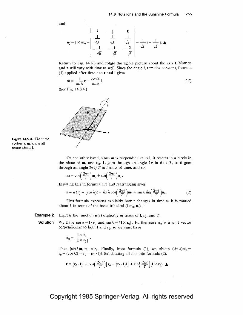
Copyright 1985 Springer-Verlag. All rights reserved
Figure 14.S.4. The three vectors v, m, and n all rotate about I.
14.S Rotations and the Sunshine Formula 755
and
1
n0 =Ix111o= ff 1
V6
j 1
ff 1
12
k
1
ff 2
V6
1 . 1 . = -1- -J. A
12 12
Return to Fig. 14.S.3 and rotate the whole picture about the axis I. Now m and n will vary with time as well. Since the angle A. remains constant, formula (1) applied after time t to rand I gives
m = _l _ r _ cos A. 1 sin A. sin A.
(l ')
(See Fig. 14.S.4.)
On the other hand, since m is perpendicular to I, it rotates in a circle in the plane of D1o and n0 . It goes through an angle 27T in time T, so it goes through an angle 2'1Tt / T in t units of time, and so
m = cos( 2;t )111o + sin(
2;t )no .
Inserting this in formula (l') and rearranging gives
r = u(t) = (cosA.)l +sin A.cos( 2;t )111o +sin A.sin( 2;t )no. (2)
This formula expresses explicitly how r changes in time as it is rotated about I, in terms of the basic trihedral (I, 111o, n0).
Example 2 Express the function u(t) explicitly in terms of I, r0 , and T.
Solution We have cos A.= I· r0 and sinA. = Ill X r0 11. Furthermore n0 is a unit vector perpendicular to both I and r0 , so we must have
IX r0
no= Ill X roll .
Thus (sinA.)n0 =IX r0 . Finally, from formula (1), we obtain (sinA.)m0 = r0 - (cos A.)l = r0 - (r0 • 1)1. Substituting all this into formula (2),
r = (r0 • 1)1 + cos( 2;r ) [ r0 - (r0 • 1)1 J + sin( 2;t )Ct x r0). A

Copyright 1985 Springer-Verlag. All rights reserved
756 Chapter 14 Curves and Surfaces
Example 3 Show by a direct geometric argument that the speed of the tip of r is (2w / T)sin A.. Verify that equation (2) gives the same formula.
Solution The tip of r sweeps out a circle of radius sin A., so it covers a distance 2w sin A. in time T. Its speed is therefore (271" sin A.)/ T (Fig. 14.S.5). From formula (2), we find the velocity vector to be
(J
Figure 14.S.5. The tip of r sweeps out a circle of radius sin t...
Figure 14.S.6. The unit vector u points from the sun to the earth at time t.
k k
~ Figure 14.S.7. At t = 0, the earth's axis is tilted toward the sun.
dr = - sin A. . 2w sin{ 2wt )Dlo + sin A. . 2w cos{ 2wt )no dt T T T T '
and its length is (since Dlo and n0 are unit orthogonal vectors)
II ! II ~ f in'A ( 2; )'<in' ( 2;') Hin'A ( 2; ) 'cot( 2;t ) = sinA. · { 2; ), as above. A.
Now we apply our study of rotations to the motion of the earth about the sun, incorporating the rotation of the earth about its own axis as well. We will use a simplified model of the earth-sun system, in which the sun is fixed at the origin of our coordinate system and the earth moves at uniform speed around a circle centered at the sun. Let u be a unit vector pointingfrom the sun to the earth; we have u = cos(2wt / Ty)i + sin(2wt / Ty)j, where ~ is the length of a year (t and ~ measured in the same units). See Fig. 14.S.6. Notice that the unit vector pointing from the earth to the sun is - u and that we have oriented our axes so that u = i when T = 0.
Next we wish to take into account the rotation of the earth. The earth rotates about an axis which we represent by a unit vector I pointing from the center of the earth to the North Pole. We will assume that I is fixed4 with respect to i, j, and k; astronomical measurements show that the inclination of I (the angle between I and k) is presently about 23.5°. We will denote this angle by a. If we measure time so that the first day of summer in the northern hemisphere occurs when t = 0, then the axis I must tilt in the direction - i, and so we must have I= cosak - sinai. (See Fig. 14.S.7.)
Now let r be the unit vector at time t from the center of the earth to a fixed point P on the earth's surface. Notice that if r is located with its base
4 Actually, the axis I is known to rotate about k once every 21,000 years. This phenomenon, called precession or wobble, is due to the irregular shape of the earth and may play a role in long-term climatic.changes, such as ice ages. See pp. 130-134 of The Weather Machine by Nigel Calder, Viking (1974).

Copyright 1985 Springer-Verlag. All rights reserved
Figure 14.S.8. The vector r is the vector from the center of the earth to a fixed location P. The latitude of Pis land the colatitude is A = 90° - !. The vector mo is a unit vector in the plane of the equator (orthogonal to I) and in the plane of I and r0 .
14.S Rotations and the Sunshine Formula 757
point at P, then it represents the local vertical direction. We will assume that P is chosen so that at t = 0, it is noon at the point P; then r lies in the plane of I and i and makes an angle of less than 90° with - i. Referring to Fig. 14.S.8, we introduce the unit vector Dlo = -(sina)k - (cosa)i orthogonal to I. We then have r0 = (cos;.\)l + (sin;.\)filo, where;.\ is the angle between I and r0 . Since ;.\ = 90° - l, where l is the latitude of the point P, we obtain the expression r0 = (sin/)1 + (cos/)filo. As in Fig. 14.S.3, let n0 =Ix Dlo·
m
Example 4 Prove that n0 = I x mo = - j.
Solution Geometrically, I x Dlo is a unit vector orthogonal to I and m0 pointing in the sense given by the right-hand rule. But I and Dlo are both in the ik plane, so IX Dlo points orthogonal to it in the direction -j (see Fig. 14.S.8).
Algebraically, I= (cosa)k - (sina)i and m0 = -(sina)k - (cosa)i, so
j IX mo= -sma 0
- cos a 0
k cos a
-sma
Now we apply formula (2) to get
r= (cos;.\)l + sin;.\cos( 2;; )mo+ sin;.\sin( 2;; )00 ,
where Td is the length of time it takes for the earth to rotate once about its axis (with respect to the "fixed stars"-i.e., our i,j, k vectors).5 Substituting the expressions derived above for;.\, I, IDo, and n0 , we get
r = sin l (cos ak - sin ai) + cos l cos( 2;; ) ( - sin ak - cos ai) - cos l sin( 2;; )j. Hence
r = -[sin/sin a+ cos/cosacos( 2;;) }- cos/sin(
2;; )i
+ [sin I cosa - cos l sin a cos( 2;; ) Jk. (3)
Example 5 What is the speed (in kilometers per hour) of a point on the equator due to the rotation of the earth? A point at latitude 60°? (The radius of the earth is 6371 kilometers.)
Solution From Example 3, the speed is s = (2'TTR/Td)sin;.\ = (27TR/Td)cosl, where R is the radius of the earth and I is the latitude. (The factor R is inserted since r is a unit vector; the actual vector from the earth's center to a point P is Rr).
5 Td is called the length of the sidereal day. It differs from the ordinary, or solar, day by about I part in 365. (Can you explain why?) In fact, Td""' 23.93 hours.

Copyright 1985 Springer-Verlag. All rights reserved
758 Chapter 14 Curves and Surfaces
Figure 14.S.9. The intensity of sunlight is proportional to sin A. The ratio of area 1 to area 2 is sinA.
Figure 14.S.10. The geometry for the formula sinA = cos(90° - A)
= -u·r.
Using Td = 23.93 hours and R = 6371 kilometers, we get s = 1673 cos/ kilometers per hour. At the equator I= 0, so the speed is 1673 kilometers per hour; at I = 60°, s = 836.4 kilometers per hour. A.
With formula (3) at our disposal, we are now ready to derive the sunshine formula. The intensity of light on a portion of the earth's surface (or at the top of the atmosphere) is proportional to sinA, where A is the angle of elevation of the sun above the horizon (see Fig. 14.S.9). (At night sinA is negative, and the intensity then is of course zero.)
Thus we want to compute sinA. From Fig. 14.S.10 we see that sinA = - u • r. Substituting u = cos(2'1Tt / ~)i + sin(2'1Tt / ~)j and formula (3) into this formula for sinA and taking the dot product gives
sin A = cos( 2~1
) [sin I sin a + cos I cos a cos( 2;; ) ]
+ sin( 2~1
) [cos I sin( 2;; ) ]
( 2'1Tt) . I . =cos ~ sm smo:
+cost[ cos( 2~t )coso:cos( 2;;) +sin( 2~t )sin( 2;;) l (4)
90° -A
-u ... ,/ .. ,,".J' ...
Sunlight
Example 6 Set t = 0 in formula (4). For what I is sinA = O? Interpret your result.
Solution With t = 0 we get
sinA = sin/sino: + cos!cosa =cos(!- a).
This is zero when/ - a= ±'IT /2. Now sinA = 0 corresponds to the sun on the horizon (sunrise or sunset), when A = 0 or 'IT. Thus, at t = 0, this occurs when I = a ± ('IT /2). The case a + ('IT /2) is impossible, since I lies between - 'IT /2 and 'IT /2. The case l = a - ('IT /2) corresponds to a point on the Antarctic Circle; indeed at t = 0 (corresponding to noon on the first day of northern summer) the sun is just on the horizon at the Antarctic Circle . ..._

Copyright 1985 Springer-Verlag. All rights reserved
14.S Rotations and the Sunshine Formula 759
Our next goal is to describe the variation of sinA with time on a particular day. For this purpose, the time variable t is not very convenient; it will be better to measure time from noon on the day in question.
To simplify our calculations, we will assume that the expressions cos(2wt /Ty) and sin(2wt /Ty) are constant over the course of any particular day; since ~ is 365 times as large as the change in t, this is a reasonable approximation. On the nth day (measured from June 21), we may replace 2wt/Ty by 2wn/365, and formula (4) gives
sinA = (sin/)P +(cos/)[ Qcos( 2;;) + Rsin(
2;;) l (5)
where P = cos(2wn/365)sina:, Q = cos(2wn/365)cosa:, and R = sin(hn/365). We will write the expression Q cos(2wt / Td) + R sin(2wt / Td) in the form
U cos[2w(t - tn)/ Td], where tn is the time of noon of the nth day. To find U, we use the addition formula to expand the cosine:
u cos( 2;: -2;:n ) = u[ cos( 2;: )cos(
2;:n ) + sin( 2;; )sin(
2;:n ) l
Setting this equal to Q cos(2wt / Td) + R sin(2wt / Td) and comparing coefficients of cos 2wt / Td and sin 2wt / Td gives
2wtn . 2wtn Ucos-- = Q and Usm-- = R.
Td Td
Squaring the two equations and adding gives
u2 = Q 2 + R 2 or U = V Q 2 + R 2 '6
while dividing the second equation by the first gives tan(2wtn/ Td) = R/ Q. We are interested mainly in the formula for U; substituting for Q and R gives
U= cos2( 2wn )coia + sin2
( 2wn )
365 365
1 - cos2( ~~; )sin
2a: .
Letting T be the time in hours from noon on the nth day so that ( t - tn) / Td = 'T /24, we may substitute into formula (5) to obtain the final formula:
. . I ( 2wn) · + I smA = sm cos 365
sma: cos 1 - cos2(
2wn )sin2a: cos( 2'1T'T ) 365 24 ' (6)
which is identical (after some changes in notation) to formula (1) on page 301.
Example 7 How high is the sun in the sky in Edinburgh (latitutde 56°) at 2 P.M. on February l?
Solution We plug into formula (6): a= 23.5°, I= 90 - 56 = 34°, n =number of days after June 21 = 225, and T = 2 hours. We get
sinA = 0.5196, so A = 31.3 °. J;,.
6 We take the positive square root because sin A should have a local maximum when t = tn.

Copyright 1985 Springer-Verlag. All rights reserved
760 Chapter 14 Curves and Surfaces
Exercises for The Supplement to Chapter 14 1. Let I= G + k)/y'2 and r 0 = (i - j)/y'2. (a) Find
mo and n0 . (b) Find r = u(t) if T = 24. (c) Find the equation of the line tangent to u(t) at t = 12 and T= 24.
2. From formula (2), verify that u(T /2) · n = 0. Also, show this geometrically. For what values oft is u( t) · n = 0?
3. If the earth rotated in the opposite direction about the sun, would Td be longer or shorter than 24 hours? (Assume the solar day is fixed at 24 hours.)
4. Show by a direct geometric construction that r = u(Td/ 4) = - sin l sin ai - cos /j +sin l cos ak. Does this formula agree with formula (3)?
Review Exercises for Chapter 14 Sketch the graphs of the conics in Exercises 1-8.
1. 4x 2 + 9y2 = 36 2. x = 2y2
3. x 2 - 4y2 = 16 4. 4x2 + I6y 2 = 81
5. l00x2 + l00y2 = I 6. y 2 = 16 + 4x2
7. x 2 - y = 14 8. 2x2 + 2y2 = 80
Sketch the graphs of the conics in Exercises 9-12. 9. 9x2 - 18x + y 2
- 4y + 4 = 0. 10. 9x 2 + 18x - y 2 + 2y - 8 = 0. 11. x 2 + 2xy + 3y2 = 14. 12. x 2 - 2xy - 3y2 = 14.
Sketch or describe the level curves for the functions and values in Exercises 13-16.
13. f(x, y) = 3x - 2y; c = 2 14. f(x, y) = x 2 - y 2; c = - I 15. f(x, y) = x 2 + xy; c = 2 16. f(x, y) = x 2 + 4; c = 85
Describe the level surfaces f( x, y, z) = c for each of the functions in Exercises 17-20. Sketch for c =I and c = 5.
17. f( x, y, z) = x - y - z 18. f(x, y,z) = x + y - 2z 19. f(x, y,z) = x 2 + y 2 + z 2 +I 20. f(x, y,z) = x 2 + 2y2 + 3z2
Sketch and describe the surfaces in Exercises 21-28. 21. x 2 + 4y2 + z 2 = I 22. x 2 + 4y2 - z 2 = 0 23. x 2 + 4y2 - z 2 = I 24. x 2 + 4y2 + z 2 = 0 25. x 2 + 4y2 - z = I 26. x 2 + 4y2 - z = 0 27. x 2 + 4y2 + z = I 28. x 2 + 4y2 + z = 0
29. This exercise concerns the elliptic hyperboloid of one sheet. An example of this type was studied in Example 6, Section 14.4. A standard form for the
5. Derive an "exact" formula for the time of sunset from formula (4).
6. Why does formula (6) for sinA not depend on the radius of the earth? The distance of the earth from the sun?
7. How high is the sun in the sky in Paris at 3 P.M. on January 15? (The latitude of Paris is 49°N).
8. How much solar energy (relative to a summer day at the equator) does Paris receive on January 15? (The latitude of Paris is 49° N).
9. How would your answer in Exercise 8 change if the earth were to roll to a tilt of 32° instead of 23.5°?
equation is
x2 y2 z2 -+---=l a2 b2 c2
(a, b, and c positive).
(a) What are the horizontal cross sections obtained by holding z constant?
(b) What are the vertical cross sections obtained by holding either x or y constant?
(c) Sketch the surface defined by
x2 y2 z2 4+1-T=l.
In a yz plane, sketch the cross-section curves obtained from this surface when x is held constantly equal to 0, 1, 2, and 3 (x = 2 is especially interesting).
30. (a) Describe the level surfaces of the function f(x,y,z)=x 2 +y2-z2. In particular, discuss the surface f(x, y, z) = c when c is positive, when c is negative, and when c is zero.
(b) Several level surfaces of f are sketched in Fig. 14.R.l. Find the value of c associated with each.
(c) Describe how the appearance of the level surfaces changes if we consider instead the function g(x, y,z) = x 2 + 2y2
- z 2•
31. Letf(x, y) = x 2 + 2y2 +I (a) Sketch the level curves f(x, y) = c for c =
-10, -1, 0, 1, 2, and 10. (b) Describe the intersection of the graph off
with the vertical planes x = 1, x = - 1, x = 2, y = 1, y = 2, y = - 1.
(c) Sketch the graph off.

Copyright 1985 Springer-Verlag. All rights reserved
x
Figure 14.R.1. Level surfaces of x 2 + y 2 - z 2.
(i)
y
32. Do as in Exercise 31 for f(x, y) = y / x, and describe the intersection of the graph of f with the cylinder of radius R (that is, r = R in cylindrical coordinates).
In Exercises 33-38, fill in the blanks and plot.
Rectangular coordinates
33. (1, - I, I) 34. (1, o. 3) 35. 36. 37. 38.
Cylindrical coordinates
(5,'7T/12,4) (8, 3'7T /2. 2)
Spherical coordinates
(3, -'7T/6,'7T/4) (10,'7T/4,'7T/2)
39. A surface is described in cylindrical coordinates by 3r2 = z 2 + I. Convert to rectangular coordinates and plot.
40. Show that a surface described in spherical coordinates by f(p, cp) = 0 is a surface of revolution.
41. Describe the geometric meaning of replacing (p, (}, cp) by (p, (} + '7T, cf>+ '7T /2) in spherical coordinates.
42. Describe the geometric meaning of replacing (p, (},</>)by (4p, (}, </>) in spherical coordinates.
43. Describe by means of cylindrical coordinates a solenoid consisting of a copper rod of radius 5 centimeters and length 15 centimeters wound on the outside with copper wire to a thickness of 1.2 centimeters. Give separate descriptions of the rod and the winding.
44. A gasoline storage tank has two spherical cap ends of arc length 56.55 feet. The cylindrical part
Review Exercises for Chapter 14 761
of the tank has length 16 feet and circumference 113.10 feet. Let (0, 0, 0) be the geometric center of the tank. See Fig. 14.R.2.
113.10 ft
Figure 14.R.2. The gasoline storage tank for Exercise 44.
(a) Describe the cylindrical part of the tank via cylindrical coordinates.
(b) Describe the hemispherical end caps with spherical coordinates. (Set up spherical coordinates using the centers of the cap ends as the origin.)
Sketch the curves or surfaces given by the equations in Exercises 45-52.
45. z = x + y 46. x 2 + 2xz + z 2
= 0 47. u(t)=3sinti+ tj+costk 48. u(t) = (sint,t + 1,2t - 1) 49. z 2 = -(x2 + y 2/4) 50. z = -(x 2 + y 2
)
51. z 2 = -x2 -3y2 +2 52. z 2 = x 2 - 4y 2
Find the equation of the line tangent to each of the curves at the indicated point in Exercises 53 and 54.
53. (t 3 + l,e-', cos('7Tt/2)); t = 1 54. (t 2
- 1, cos t 2, t 4
); t = fii Find the velocity and acceleration vectors for the curves in Exercises 55-58.
55. u 1(t) = e'i + sintj + costk. 2
56. ui(t) = _t_ i + tj + k. 1 + t1
57. u(t) = u 1(t) + u 2(t), where u 1 and u 2 are given in Exercises 55 and 56.
58. u(t) = u 1(t) X ui(t), where u 1 and u 2 are given in Exercises 55 and 56.
59. Write in parametric form the curve described by the equations x - 1 = 2y + 1 = 3z + 2.
60. Write the curve x = y 3 = z 2 + 1 in parametric form.
61. Find the arc length of u(t) = ti+ Int j + 2/2tk; 1 < t < 2.
62. Express as an integral the arc length of the curve x 2 = y 3 = z 5 between x = 1 and x = 4. (Find a parametrization.)
63. A particle moving on the curve u(t) = 3t2i -sin tj - e'k is released at time t = 1 and flies off on a tangent. What are its coordinates at time t = I?
64. A particle is constrained to move around the unit circle in the xy plane according to the formula (x, y, z) = (cos(t2
), sin(t2), 0), t > 0.

Copyright 1985 Springer-Verlag. All rights reserved
762 Chapter 14 Curves and Surfaces
(a) What are the velocity vector and speed of the particle as functions of t?
(b) At what point on the circle should the particle be released to hit a target at (2, 0, O)? (Be careful about which direction the particle is moving around the circle.)
(c) At what time t should the release take place? (Use the smallest t > 0 which will work.)
(d) What are the velocity and speed at the time of release?
(e) At what time is the target hit? 65. A particle of mass m is subject to the force law
F = - kr, where k is a constant. (a) Write down differential equations for the
components of r(t). (b) Solve the equations in (a) subject to the
initial conditions r(O) = 0, r'(O) = 2j + k. 66. Show that the quantity
; II ~~ /( + ~ r . r is independent of time when a particle moves under the force law in Exercise 65.
67. Find the curvature of the ellipse 4x2 + 9y 2 = 16.
Figure 14.R.3. Yosemite Valley (portion). (U.S. Department of Interior Geological Survey.)
* 68. Let r = u(t) be a curve in space and N be its principal normal vector. Consider the "parallel curve" r = µ(t) = u(t) + N(t), where u(t) is the displacement vector to P(t) from a fixed origin. (a) Under what conditions does µ(t) have zero
velocity for some t0 ? [Hint: Use the Frenet formulas, Exercise 25, Section 14.7]
(b) Find the parametric equation of the parallel curve to the ellipse (±cost, 4 sin t, 0).
69. Find a formula for the curvature of the graph y = j(x) in terms off and its derivatives.
70. The contour lines on a topographical map are the level curves of the function giving height above sea level as a function of position. Figure 14.R.3 is a portion of the U.S. Geological Survey map of Yosemite Valley. There is a heavy contour line for every 200 feet of elevation and a lighter line at each 40-foot interval between these. (a) What does it mean in terms of the terrain
when these contour lines are far apart? (b) What if they are close together? (c) What does it mean when several contour
lines seem to merge for a distance? Is eleva-

Copyright 1985 Springer-Verlag. All rights reserved
tion really a function of position at such points? (Look at the west face of Half Dome. Does this seem like a good direction from which to climb it?)
( d) Sketch a cross section of terrain along a north-south line through the top of Half Dome.
(e) A hiker is not likely to follow the straight north-south path in part (d) and is probably more interested in the behavior of the terrain along the trail he or she will follow. The 3-mile route from the Merced River (altitude approximately 6100 feet) to the top of Half Dome (approximately 8842 feet) along the John Muir and Half Dome Trails has been emphasized in Fig. 14.R.3. Show how a cross section of the terrain along this trail behaves by plotting altitude above sea level as a function of miles along the trail. (A piece of string or flexible wire may be of aid in measuring distances along the trail.)
* 71. Find the curvature of the "helical spiral" (t, t cost, t sin t) fort> 0. Sketch.
*72. Describe the level curves f(x, y) = c for each of the following functions. In particular, discuss any special values of c at which the behavior of the level curves changes suddenly. Sketch the curves for c = - 1, 0, and I. (a) f(x, y) = x + 2y; (b) f(x, y) = x2 - y2; (c) f(x, y) = y2 - x2; (d) f(x, y) = x2 + y2; (e) f(x, y) = xy; (f) f(x, y) = y - 2x2.
*73. (a) Write in parametric form the curve which is the intersection of the surfaces x 2 + y 2 + z2
= 3 andy =I. (b) Find the equation of the line tangent to this
curve at (1, I, I). (c) Write an integral expression for the arc
length of this curve. What is the value of this integral?
Review Exercises for Chapter 14 763
* 74. Let n be a positive integer and consider the curve
x = c6s t cos( 4nt) }
y = c~stsin(4nt) - ~.;; t < ~,
z = smt
(a) Show that the path traced out lies on the surface of the sphere of radius I centered at the origin.
(b) How many times does the curve wind around the z axis?
(c) Where does the curve cross the xy plane? (d) Sketch the curve when n = I and when
n = 2. * 75. Let u1 and u2 be unit vectors, and define the
curve u( t) by
(a) (b) (c)
(d)
( ) U1COS t + U2sin t
u t =-------lln1COS t + U2sin t11 ,
Find u(O) and u('TT /2). On what surfaces does u(t) lie for all t? Find, by geometry, the arc length of the curve u(t) for 0 < t < 'TT /2. Express the arc length of the curve u(t) for 0 < t < 'TT /2 as an integral.
(e) Find a curve u 1(t) which traverses the same
*76 (a)
(b)
path as u(t) for 0 < t < 'TT /2 and such that the speed llu](t)ll is constant. Show that the hyperboloid x 2 + y 2 - z2 = 4 is a ruled surface by finding two straight lines lying in the surface through each point. [Hint: Let (x0 , y 0 , z0) lie on the surface; write the equation of the line in the form x = x0 +at, y = y 0 +ht, z = z0 + t; write out x 2 + y 2 - z2 = 4 using xJ + yJ - zJ = 4 to obtain two equations for a and b representing a line and a circle in the (a, b) plane. Show that these equations have two solutions by showing that the distance from the origin to the line is less than the radius of the circle.] I-s the hyperboloid x 2 + y 2 - z2 = - 4 a ruled surface? Explain.
(c) Generalize the results of parts (a) and (b).

Copyright 1985 Springer-Verlag. All rights reserved
Chapter15
Partial Differentiation
A function of several variables can be differentiated with respect to one variable at a time.
The rate of change of a function of several variables is not just a single function, since the independent variables may vary in different ways. All the rates of change, for a function of n variables, are described by n functions called its partial derivatives. This chapter begins with the definition and basic properties of partial derivatives. Methods for computation, including the chain rule, are presented along with a geometric interpretation in terms of tangent planes. The next chapter continues the development with topics including implicit differentiation, gradients, and maxima and minima.
15.1 Introduction to Partial Derivatives The partial derivatives of a function of several variables are its ordinary derivatives with respect to each variable separately.
In this section we define partial derivatives and practice computing them. The geometric significance of partial derivatives and their use in computing tangent planes are explained in the next section.
Consider a function f ( x, y) of two variables. If we treaty as a constant, f may be differentiated with respect to x. The result is called the partial derivative off with respect to x and is denoted by fx. If we let z = f(x, y), we write
fx = ~~ · These symbols1 are analogous to those we used m one-variable calculus:
f'(x) = dy/dx.
The partial derivative with respect toy is similarly defined by treating x as a constant and differentiatingf(x, y) with respect toy.
1 The symbol a seems to have first been used by Clairaut and Euler around 1740 to avoid confusion with d. The notation Dxf or D 1 f for fx is also used.

Copyright 1985 Springer-Verlag. All rights reserved
766 Chapter 15 Partial Differentiation
Example 1 (a) If f(x, y) = xy + excos y, .compute fx and fy. (b) For fas in (a), calculate JAl,w /2).
(c) If z = xy3 + xy4 - exy2, calculate ~~ and ~; .
Solution (a) Treatingy as a constant and differentiating with respect to x, we get
fx( x, y) = y + excos y.
Figure 15.1.1. The partial derivatives fx and fy are limits of difference quotients along the horizontal and vertical paths shown here.
Differentiating with respect toy and considering x as a constant gives
fy(x,y) = x - exsiny.
(b) Substituting x = 1 and y = w /2, we get
fx(l,w/2) = w/2 + e 1cos(w/2) = w/2.
(c) Here we again hold y constant and calculate the x derivative:
~~ = 2xy3 + 3xy4 - y 2exy'.
Similarly,
~; = 3xy2 + 4x}i3 - 2yxexy'. •
In terms of limits, partial derivatives are given by
. f(x+~x,y)-f(x,y) fx(x,y)= hm A
L\.x-40 uX
and
. f(x, y + ~y) - f(x, y) fy(x,y) = hm ~ .
L\.y-40 :Y
See Fig. 15.1.1. y y
y +L'>y
y s10s•1u(x+Lix,y) Y (x,y)
x x+L'>x x
I (x,y +L'>y)
(x,y)
x x
Partial derivatives of functions f ( x, y, z) of three variables are defined similarly. Two variables are treated as constant while we differentiate with respect to the third.
Example 2 (a) Let f(x, y, z) = sin(xy / z). Calculate fz(x, y, z) and .fz(l, 2, 3). (b) Evaluate
a ay -Jx2 + y2 + z2
at (0, 1, 1). (c) Write the result in (b) as a limit.
Solution (a) We differentiate sin(xy / z) with respect to z, thinking of x and y as constants; the result is
fz( x, y, z) =cos( xy / z)( - xy / z2) = -( xy / z2)cos( xy / z).

Copyright 1985 Springer-Verlag. All rights reserved
15.1 Introduction to Partial Derivatives 767
Substituting (1, 2, 3) for (x, y, z) gives
1·2 (1•2) 2 (2) .fz(l,2,3) = - 32 cos -3- = - 9 cos 3 .
(b) Treating x and z as constants, and using the chain rule of one-variable calculus,
a = _1_ (x2 + y2 + z2)-l/2 ay -/x2 + y2 + z2 ay
At (0, 1, 1) this becomes
= (- ~ )(x2 + y2 + z2f3/2. 2y
-y 3/2 .
(x2 + y2 + z2)
-1 = ___::_!_ (02+ 12+ 12)3/2 2[i
( c) In general,
f(x, y + Ay,z) - f(x, y,z) lim A.v = fy(x,y,z).
Ll.y~O .:..1_,
In case (b ), this becomes
}f":o d j(l + ~)' + I - ~ l ~ -2~ A
Partial Differentiation If f is a function of several variables, to calculate the partial derivative with respect to a certain variable, treat the remaining variables as constants and differentiate as usual by using the rules of one-variable calculus.
If z = f(x, y) is a function of two variables, the partial derivatives are denotedfx = az/ax andfy = az/ay.
If u = j(x, y,z) is a function of three variables, the partial derivatives are denotedfx = au/ax,fy = au/ay, and.fz = au/az.
As in one-variable calculus, the letters for the variables do not always have to bex,y,z.
Example 3 If h = rs2sin(r2 + s2), find ah/as.
Solution Holding r constant, we get
~; = 2rs sin(r2 + s2) + rs2 • 2s · cos(r2 + s2)
= 2rs[ sin(r2 + s2) + s2cos(r2 + s2) J. £

Copyright 1985 Springer-Verlag. All rights reserved
768 Chapter 15 Partial Differentiation
Partial derivatives may be interpreted in terms of rates of change, just as derivatives of functions of one variable.
Example 4 The temperature (in degrees Celsius) near Dawson Creek at noon on April 15, 1901 is given by T = - (0.0003)xy + (0.9307)y, where x and y are the latitude and longitude (in degrees). At what rate is the temperature changing if we proceed directly north? (The latitude and longitude of Dawson Creek are x = 55.7° andy = 120.2°.)
Solution Proceeding directly north means increasing the latitude x. Thus we calculate
~: = -(0.0003) · 2xy = -(0.0003) · 2 · (55.7) · (120.2) ~ -4.017.
So the temperature drops as we proceed north from Dawson Creek, at the instantaneous rate of 4.0l 7°C per degree of latitude . .A.
Since the partial derivatives are themselves functions, we can take their partial derivatives to obtain higher derivatives. For a function of two variables, there are four ways to take a second derivative. If z = j(x, y), we may compute
J ( ) a ( az ) a2z r a ( az ) a
2z
xx x,y =ax ax = ax2 ' Jyy(x,y)= ay ay = ay2 '
f a ( az ) a2z
J xy ( x' y) = a y ax = a y ax ' f x =_l_(~)=_fr_ Jyx( 'y) ax ay ax ay .
Example 5 Compute the second partial derivatives of z = xy2 + ye-x + sin(x - y).
Solution We compute the first partials:
az 2 -x + ( ) ax = y - ye cos x - y
and
~; = 2xy + e-x - cos(x - y).
Now we differentiate again:
a2z - x . ( ) a2
z 2 . ax2 =ye - sm x - y ' ay2 = x - sm(x - y),
a2z a ( az ) 2 -x . ( -- = - - = y - e + sm x - y),
ayax ay ax a2
z a ( a z ) 2 - x · -- = - - = y - e + sm( x - y) . .A.. ax ay ax ay
Example 6 (a) If u = ycos(xz) + xsin(yz), calculate a2u/axaz and a2u/azax. (b) Let j(x,y,z) = exy + zcosx. Find.fzx andfxz·
Solution (a) We find au/ax= - yz sin(xz) + sin(yz) and au/az = - xy sin(xz) + xy cos(yz). Thus
a2u az ax = - y sin( xz) - xyz cos( xz) + y cos(yz).
Differentiation of au/az with respect to x yields
a2u axaz = -ysin(xz)- xyzcos(xz) + ycos(yz).
(b) fx(x, y, z) = yexy - z sinx; fz(x, y, z) = cosx; .fzx(x, y, z) =(a /ax)(cosx) = - sinx; fxz(x, y, z) =(a /az)(yexy - z sinx) = - sinx . .A

Copyright 1985 Springer-Verlag. All rights reserved
y
Figure 15.1.2. The disk Dr(x0 , y 0) consists of the shaded region (excluding the solid circle).
15.1 Introduction to Partial Derivatives 769
In the preceding examples, note that the mixed partials taken in different orders, like o2z I ax a y and o2z I a y ax' or fxz and fzx' are equal. This is no accident.
Theorem: Equality of Mixed Partial Derivatives
If u = j(x, y) has continuous second partial derivatives, then the mixed partial derivatives are equal; that is,
o2u - o2u ox oy - oy ax or hx = fxy.
Similar equalities hold for mixed partial derivatives of functions of three variables.
L. Euler discovered this result around 1734 in connection with problems in hydrodynamics. To prove it requires the notions of continuity and limit for functions of two variables.2
Let us write d((x, y), (x0 , y 0)) = VC x - x0)2 + (y - y 0 )
2 for the distance
between (x,y) and (x0 ,y0), with a similar notation d((x,y,z),(x0 ,y0 ,z0)) in x space. The disk Dr(x0 , y 0) of radius r centered at (x0 , y 0) is, by definition, the
set of all (x,y) such that d((x,y),(x0 ,y0)) < r, as shown in Fig. 15.1.2. The limit concept now can be defined by the same e, 8 technique as in one variable calculus.
The e, 8 Definition of Limit Suppose that f is defined on a region which includes a disk about (x0 , y 0), but need not include (x0 , y 0) itself. We write
lim f(x, y) =I ( x ,y )~( xo,yo)
if, for every e > 0, there is a 8 > 0 such that lf(x, y) - II < e whenever 0 < d((x, y), (x0 , y 0)) < 8. A similar definition is made for functions of three variables.
The e, 8 definition of limit may be rephrased as follows: for every e > 0, there is a 8 > 0 such that lf(x, y) - !I < e if (x, y) lies in D8 (x0 , y 0).
The similarity between this definition and the one in Chapter 11 should be evident. The rules for limits, including rules for sums, products, and quotients, are analogous to those for functions of one variable.
Example 7 Prove the "obvious" limit, lim(x,y)~(xo, Yolx = x 0, using e's and 8's.
Solution Let e > 0 be given and let j(x, y) = x and I= x 0 • We seek a number 8 > 0 such that lf(x, y) - !I < e whenever d((x, y), (x0 , y 0)) < 8, that is, such that
Ix - xol < e whenever vex - Xo)2 + (y - Yo) 2 < 8. However, note that
Ix - Xol =vex - xof <V(x - Xo)2 + (y - Yo)2'
so if we choose 8 = e, d((x, y), (x0 , y 0)) < 8 will imply Ix - x0 1 < e . .A
2 If you are not interested in the theory of calculus, you may skip to p. 772. Consult your instructor.

Copyright 1985 Springer-Verlag. All rights reserved
770 Chapter 15 Partial Differentiation
Example 8
Solution
. . x 3 + 2x2 + xy2 + 2y2 Fmd hm(x,y)--+(O,O) 2 + 2
x y
The numerator and denominator vanish when (x, y) = (0, 0). The numerator factors as (x 2 + y 2)(x + 2), so we may use the replacement rule and algebraic rules to get
lim (x,y)~(O,O)
(x 2 + y 2)(x + 2) 2 2 = lim ( x + 2) = 0 + 2 = 2 . .._
X + y (x,y)~(O,O)
Example 9 Show that
lim JL i/x2 + y 2 (x,y)~(O,O) ax
does not exist. [Hint: Look at the limits along the x andy axes.]
Solution (a /ax)i/x2 + y 2 = x / i/x2 + y 2 if (x, y) * (0, 0). Thus
lim JL i/ x 2 + y 2 = lim x . (x,y)~(O,O) ax (x,y)~(O,O) i/x2 + y2
If we approach (0, 0) on they axis-that is, along points (0, y)-we get zero. Thus the limit, if it exists, is zero. On the other hand, if we approach (0, 0)
along the positive x axis, we have y = 0 and x > O; then x/Vx2 + y 2 = 1
because x / R = 1, so the limit is 1. Since we obtain different answers in different directions, the actual limit cannot exist. .._
We can base the concept of continuity on that of limits, just as we did in Section 1.2.
Definition of Continuity Let f be defined in a disk about (x0 , y 0). Then we say f is continuous at (xo,Yo) if
lim f(x,y) = f(xo,Yo)· (x,y)~(xo,yo)
There is a similar definition for functions of three variables.
Most "reasonable" functions of several variables are continuous, although this may not be simple to prove from the definition. Here is an example of how to do this.
Example 10 (a) If f(x) and g(y) are continuous functions of x and y, respectively, show that h(x, y) = f(x)g(y) is continuous. (b) Use (a) to show that excos y is continuous.
Solution (a) We must show that for any (x0 , y 0), lim(x,y)--+(xo,Yoif(x)g(y) = j(x0)g(y0).
To this end, we manipulate the difference:
/f(x)g(y) - f(xo)g(yo)/
= /f(x)g(y) - f(xo)g(y) + f(xo)g(y) - f(xo)g(yo)/

Copyright 1985 Springer-Verlag. All rights reserved
15.1 Introduction to Partial Derivatives 771
< l(J(x) - f(xo))g(y)I + lf(xo)(g(y) - g(Yo))I
= lf(x) - f(xo)l I g(y)I + lf(xo)l I g(y) - g(yo)I
< If( x) - f( Xo)l(I g(Yo)I + I g(y) - g(yo)I) + If( Xo)l I g(y) - g(yo)I
= If( x) - f(xo)l I g(yo)I + If( Xo)l I g(y) - g(yo)I
+ lf(x) - f(xo)l I g(y) - g(Yo)I.
Now let e > 0 be given. We may choose e1 > 0 so small that we have the inequality e 1(1 g(y0 ) I + lf(y0)1) + e~ < e, by letting e1 be the smaller of
E and 1. I g(yo)I + lf(Yo)I + 1
Since f and g are continuous, there exists 81 > 0 such that, when Ix - x0 1 < 81,
lf(x) - f(x0)1 < e1, and there exists 82 such that when IY - Yol < 82 , we have the inequality I g(x) - g(x0)1 < e1• Let 8 be the smaller of 81 and 82 •
Now if d((x, y), (x0 , y 0)) < 8, we have Ix - x0 1 < 8 < 81 and IY - Yol < 8 < t2. so
If( x) g(y) - f( Xo) g(yo)I < If( x) - f( Xo)l I g(yo)I + If( xo)l I g(y) - g(yo)I
+ lf(x)- f(xo)l lg(y)- g(yo)I
< E1I g(yo)I + lf(xo)le1 + E1 • E1 < E.
Thus we have proven that lim(x,y)~(xo.Yo) = f(x 0)g(y0), so f(x)g(y) is continuous. (b) We know from one-variable calculus that the functions f(x) =ex and g(y) =cosy are differentiable and hence continuous, so by part (a), f(x)g(y) is continuous. A.
Using the ideas of limit and continuity, we can now give the proof of the equality of mixed partials; it uses the mean value theorem for functions of one variable.
Proof of the Consider the expression
equality of f( xo +Ax, Yo+ Ay) - f( Xo +Ax, Yo) - f( Xo' Yo+ Ay) + f( Xo, Yo)· (1) mixed partial
derivatives We fix y 0 and Ay and introduce the function
g( x) = f( x, Yo+ Ay) - f( x, Yo),
so that the expression (I) equals g(x0 +Ax) - g(x0). By the mean value theorem for functions of one variable, this equals g'(.X)Ax for some x between x0 and x0 +Ax. Hence (1) equals
[ ~~ (x, Yo+ Ay) - ~~ (x, Yo) ]Ax.
Applying the mean value theorem again, we get, for (1 ),
a2z c- -) A A ay ax x, y ux uy.
Since a2z/ayax is continuous and (.X,ji)~(x0,y0) as (Ax,Ay)~(O,O), it follows that
a2z ay ax (xo' Yo)
lim (Lh,Lly)->(0,0)
[f(xo +Ax, Yo+ Ay) - f(xo +Ax, Yo) - f(xo' Yo+ Ay) + f(xo' Yo)] AxLiy
(2)

Copyright 1985 Springer-Verlag. All rights reserved
772 Chapter 15 Partial Differentiation
z
(a)
z
,/
(b)
Figure 15.1.3. Moving water in a narrow tank shown at two different instants of time.
Figure 15.1.5. The derivative g'(y0) of the function g(y) = j(t0 , y) represents the slope of the water's surface at time t0
and position y 0 •
y
y
The right-hand side of formula (2) is symmetric in x and y, so that in this derivation we can reverse the roles and x and y. In other words, in the same manner we prove that a2z /ax ay is given by the same limit, and so we obtain the desired result: the mixed partials are equal. •
Supplement to Section 15.1: Partial Derivatives and Wave Motion
Two of the most important problems in the historical development of partial differentiation concerned wave motion and heat conduction. Here we concentrate on the first of these problems. (See also Exercises 71 and 72.)
Consider water in motion in a narrow tank, as illustrated in Fig. 15.1.3. We will assume that the motion of the water is gentle enough so that, at any instant of time, the height z of the water above the bottom of the tank is a function of the position y measured along the long direction of the tank; this means that there are no "breaking waves" and that the height of water is constant along the short direction of the tank. Since the water is in motion, the height z depends on the time as well as ony, so we may write z = f(t, y); the domain of the function J consists of all pairs ( t, y) such that t lies in the interval of time relevant for the experiment, and a < y < b, where a and b mark the ends of the tank.
We can graph the entire function J as a surface in (t, y,z) space lying over the strip.a < y < b (see Fig. 15.1.4); the section of this surface by a plane
Figure 15.1.4. The motion of the water is depicted by
A slice at t = t0
agraphin(t,y,z)space; Y
sections by planes of the form t = t0 show the . configuration of the water / at various instants of timYi
of the form t = t0 is a curve which shows the configuration of the water at the moment t0 (such as each of the "snapshots" in Fig. 15.1.3). This curve is the graph of a function of one variable, z = g(y), where g is defined by g(y) = f(t 0 , y). If we take the derivative of the function g at a pointy0 in (a,b), we get a number g'(y0) which represents the slope of the water's surface at the time t0 and at the location y 0 . (See Fig. 15.1.5.) It could be observed as the slope of a small stick parallel to the sides of the tank floating on the water at that time and position.
z
a
The slope of this line is g' (y 0 )
Yo b y

Copyright 1985 Springer-Verlag. All rights reserved
15.1 Introduction to Partial Derivatives 773
This number, g'(y0), is obtained from the function f by: I. Fixing t at the value t0 .
2. Differentiating the resulting function of y. 3. Setting y equal to y 0 .
The number g'(y0) is just fy(t0 , y 0).
We can also define the partial derivative off with respect to t at (t0 , y0);
it is obtained by: I. Fixing y at the value Yo· 2. Differentiating the resulting function of t. 3. Setting t equal to t0 •
The result is ft(t 0 , y 0). In the first step, we obtain the function h(t) = f(t, y 0),
which represents the vertical motion of the water's surface observed at the fixed position y 0 . The derivative with respect to t is, therefore, the vertical velocity of the surface at the position y 0 . It could be observed as the vertical velocity of a cork floatir~g on the water at that position. Finally, setting t equal to t0 merely involves observing the velocity at the specific time t0 .
Exercises for Section 15.1 Compute fx and fy for the functions in Exercises 1-8 and evaluate them at the indicated points.
I. f(x, y) = xy; (I, 1)
2. f(x, y) = x/y; (I, I) 3. f(x, y) = tan- 1(x - 3y2); (1, 0)
4. f(x, y) = -jx2 + y 2 ; (1, - 1)
5. j(x, y) = exYsin(x + y); (0, 0) 6. f(x, y) = ln(x2 + y 2 + l); (0, 0) 7. f(x,y)= 1/(x3 + y 3
); (-1,2) 8. j(x, y) = e-x'-Y
2; (I, -1)
Compute fx, fy, and f, for the functions in Exercises 9-12, and evaluate them at the indicated points.
9. f(x, y, z) = xyz; (I, I, 1)
10. j(x, y, z) = -/x2 + y 2 + z 2 ; (3, 0, 4)
11. f(x, y, z) = cos(xy 2) + e3xyz; ( 7T, I, I)
12. f(x, y, z) = xYz; (1, 1, 0) Find the partial derivatives az/ax and az/ay for the functions in Exercises I 3-16.
13. z = 3x 2 + 2y2 14. z = sin(x2 - 3xy) 15. z = (2x 2 + 7 xy)/3xy 16. z = xy2e2xy
Find the partial derivatives au/ax, au/ay, and au/az in Exercises 17-20.
17. U = e-xyz(xy + xz + yz) 18. u = sin(xy2z 3
)
19. u = excos(yz2)
20. u = (xy 3 + ez)/(x3 y - ez) Compute the indicated partial derivatives in Exercises 21-24.
21. a~ ( ;:: ~ ~ ) 22. aJu (uvw - sin(uvw))
23. aab (mx + b2)8
In Exercises 25-28, let
f(x, y) = 3x 2 + 2sin(x/y2) + y 3(1 - ex)
and find the indicated quantities. 25. fx(2, 3) 26. fxCO, I) 27. fy(l, l) 28. fy(- 1, - I)
29. Let z = (sinx)e-xY. (a) Find az/ay. (b) Evaluate az/ay at the following four points:
(0, 0), (0, 7T /2), ( 7T /2, 0), and ( 7T /2, 7T /2). 30. Let u = (xy / z)cos(yz).
(a) Find au/az. (b) Evaluate au/az at (l,7T, I), (0,7r/2, I), and
(I, 7T, 1/2). Let g(t,u,v) = ln(t + u + v)- tan(tuv) and find the indicated quantities in Exercises 31-36.
31. g,(0,0, 1) 32. g,(1,0,0) 33. gu(l,2,3) 34. gu(2,3, I) 35. gv(- J, 3, 5) 36. gv(- J, 5, 3)
In Exercises 37-40, compute the indicated partial deriv-atives
37. l_ estu'
as
39. a ( cost..µ, ) at.. i+t..2+µ,2
38. l_ ( _!_ 7Tr2h) ar 3
40. aaa (bed)
41. If f(x, y,z) is a function of three variables, express fz as a limit.
42. Find . 3+(x+y+~y)2z-(3+(x+y)2z)
hm t>y~o ~y
43. In the situation of Example 4, how fast is the temperature changing if we proceed directly west? (The longitude y is increasing as we go west.)

Copyright 1985 Springer-Verlag. All rights reserved
77 4 Chapter 15 Partial Differentiation
44. Chicago Skate Company produces three kinds of roller skates. The cost in dollars for producing x, y, and z units of each, respectively, is c(x, y,z) = 3000 + 27x + 36y + 47z. (a) The value of ac /ax is the change in cost
due to a one unit increase in production of the least expensive skate, the levels of production of the higher-priced units being held fixed. Find it.
(b) Find ac/az, and interpret. 45. If three resistors R 1, R 2, and R 3 are connected in
parallel, the total electrical resistance is determined by the equation
_!_=__!_+_!_+__!_. R R 1 R2 R3
(a) What is aR/aR 1? (b) Suppose that R 1 , R 2, and R 3 are variable
resistors set at 100, 200, and 300 ohms, respectively. How fast is R changing with respect to R 1 ?
46. Consider the topographical map of Yosemite Valley in Fig. 14.R.3. Let r represent the eastwest coordinate on the map, increasing from west to east. Lets be the north-south coordinate, increasing as you go north. (East is the positive r direction, north the positives direction.) Leth be the elevation above sea level. (a) Explain how ah/ar and ah/as are related
to the distances between contour lines and their directions.
(b) At the center of the letter o in Half Dome, what is the sign of ah/ar? of ah/as?
In Exercises 47-50, find the partial derivatives a2z/ax2,
a2z/axay, a2z/ayax and a2z/ay2 for each of the functions in the indicated exercise.
47. Exercise 13 48. Exercise 14 49. Exercise 15 50. Exercise 16
51. Let j(x, y,z) = x}i + xy2 + yz2. Findfxy•fyz,fw
andfxyz· 52. Let z = xy3 - x 8 + y 4
.
(a) Compute a3z/ay ax ax, a3z /ax ay ax, and a3z/ax ax ay.
(b) Compute a3z/ax ay ay, a3z/ay ax ay, and a3z/ayayax.
Compute a2u/ax2, a2u/ay ax, a2u/ay 2
, and a2u/ax ay for each of the functions in Exercises 53-56. Check directly the equality of mixed partials.
53. u = 2xy/(x2 + y 2)2
54. u = cos(xy2)
55. u = e-xy2 + y 3x 4
56. u = l/(cos2x + e-Y)
57. Prove, using e's and S's, that lim(x,y)->(x0,y0)Y =Yo·
58. Prove, using e's and S's, that lim(x,y)->(xo.Yo)(x + y) = Xo +Yo·
In Exercises 59-66, evaluate the given limits exist (do not attempt a precise justification).
if they
1. xy + y3
59. Im (x,y)->(0,0) x 2 + y 2
1. x+ y 1m 2
(x,y)->(Ll) (x - l) + 1 60.
61. lim x}i + y3 + x2 + y2
(x,y)->(2,3) -Jx2 + Y2
62. . 4x2 + 3y2 + x3y3
hm (x,y)->(O,O) x2 + y2 + xy4
63. lim excos('1Ty) (x,y)->(1,1)
64. Jim exycos('ITxy) (x,y)->(0,1)
65. lim sin(xy) (x,y)->(0,0)
66. lim l (x,y)->(O,O) 1 + ln( I + 1 / ( x 2 + y 2))
67. Let j(x, y) = x 2 + y 2 and suppose that (x, y) moves along the curve (x(t), y(t)) =(cost, e'). (a) Find g(t) = j(x(t), y(t)) and use your for
mula to compute g'(t0).
(b) Show that this is the same as
fx(x(t0 ), y(to)) · x'(to) + fy(x(to), y(to)) · y'(to)·
68. Let j(x, y, z) = x 2 + 2y - z and suppose the point (x, y,z) moves along the parametric curve (l,t,t 2).
(a) Let g(t) = j(l,t,t2) and compute g'(t). (b) Show that your answer in (a) is equal to
dx f, dy f dz fx dt + Y dt + z dt .
69. A function u = j(x, y) with continuous second partial derivatives satisfying Laplace's equation
a2u a2u -+-=0 ax2 ay2
is called a harmonic function. Show that the function u(x, y) = x 3 - 3xy2 is harmonic.
70. Which of the following functions satisfy Laplace's equation? (See Exercise 69). (a) j(x, y) = x 2 - y 2; (b) f(x, y) = x2 + y2; (c) j(x, y) = xy; (d) j(x, y) = y 3 + 3x}i; (e) j(x, y) = sinx cosh y; (f) j(x, y) = exsin y.
71. Let f and g be differentiable functions of one variable. Set <p = j(x - t) + g(x + t). (a) Prove that <p satisfies the wave equation:
a2<p/a12 = a2<p/ax 2.
(b) Sketch the graph of <p against t and x if j(x) = x 2 and g(x) = 0.

Copyright 1985 Springer-Verlag. All rights reserved
72. (a) Show that function g(x,t)=2+e- 1sinx satisfies the heat equation: g, = gxx. (Here g(x, t) represents the temperature in a rod at position x and time t.)
(b) Sketch the graph of g fort;;;. 0. [Hint: Look at sections by the planes t = 0, t = 1, and t = 2.]
(c) What happens to g(x, t) as t-+ oo? Interpret this limit in terms of the behavior of heat in a rod.
73. The productivity z per employee per week of a company depends on the size x of the labor force and the amount y of investment capital in millions of dollars. A typical formula is z(x, y) = 60xy - x 2 - 4y2. (a) The value of az/ax at x = 5, y = 3 is the
marginal productivity of labor per worker at a labor force of 5 people and investment level of 3 million dollars. Find it.
(b) Find az/ay at x = 5,y = 3, and interpret. 74. The productivity z of a company is given by
z(x, y) = lOOxy - 2x2 - 6y2 where x X 103 people work for the company, and the capital investment of the company is y million dollars. (a) Find the marginal productivity of labor
az/ax. This number is the expected change in production for an increase of 1000 staff with fixed capital investment.
15.2 Linear Approximations and Tangent Planes 775
(b) Find az/ay when x = 5 and y = 3. Interpret.
* 75. Show that . a 2 2 2 1/3 hm -(x+y+z)
(x,y,z)~(0,0,0) az
does not exist. *76. Let
{
xy(x2 - y2)
f(x, y) = x2 + y2 '
0,
(x,y)7"(0,0),
(x, y) = (0, 0).
(a) If (x, y) 7" (0, 0), compute fx and fy. (b) What is the value of f(x, 0) and f(O, y)? ( c) Show that fx (0, 0) = 0 = fy (0, 0).
* 77 Consider the function fin Exercise 76. (a) Show that fx(O, y) = - y when y 7" 0. (b) What is fy(x, 0) when x 7" O? (c) Show that fyx(O, 0) = 1 and fxy(O, 0) = - 1.
[Hint: Express them as limits.] (d) What went wrong? Why are the mixed
partiaJs not equal? * 78. Suppose that f is continuous at (x0 , y 0) and
f(x0 , y 0) > 0. Show that there is a disk about (x0 , y 0) on which f(x, y) > 0.
15.2 Linear Approximations and Tangent Planes The plane tangent to the graph of a function of two variables has two slopes.
In the calculus of functions of one variable, the simplest functions are the linear functions /(x) = mx + b. The derivative of such a function is the constant m, which is the slope of the graph or the rate of change of y with respect to x. If f(x) is any differentiable function, its tangent line at x 0 is the graph of the linear approximation y = f(x0) + f'(x0)(x - x 0).
To extend these ideas to functions of two variables, we begin by looking at linear functions of the form z = l(x, y) =ax+ by+ c, whose graphs are planes. Such a plane has two "slopes," the numbers a and b, which determine the direction of its normal vector - ai - bj + k (see Section 13.4). These slopes can be recovered from the function I as the partial derivatives Ix = a and~= b. By analogy with the situation for one variable, we define the linear approximation at (x0 , y 0) for a general function f of two variables to be the linear function
I( x, Y) = f( Xo, Yo) + fx( Xo, Yo)( x - Xo) + fy( Xo' Yo)(y - Yo),
which is of the form ax + by + c with
a= fx( x 0 , y 0), b = fy( x 0 , y 0), and
c = f( Xo, Yo) - Xofx( Xo, Yo) - Yofy( Xo, Yo)·

Copyright 1985 Springer-Verlag. All rights reserved
776 Chapter 15 Partial Differentiation
The function I is the unique linear function which has at (x0 , y 0) the same value and the same partial derivatives as J. The graph
z = f(xo,Yo) + f~(xo,Yo)(x - Xo) + J;,(xo,Yo)(y- Yo) (1)
of the linear approximation is a plane through (x0 , y 0 , f(x 0 , y 0)), with normal vector -fAxo, Yo)i - fy(x 0 , y0 )j + k; it is called the tangent plane at (x 0 , y0 ) to the graph off (see Fig. 15.2.1).
z
Normal vector Tangent plane
z=f(x,y) Figure 15.2.1. The tangent plane at (x0 , y 0) to the graph z = j(x, y) has the equation z = j(xo, Yo) + fxCxo, Yo)(x - Xo) + fy(xo, Yo)(y - Yo)· A vector normal to the
y
plane is
n = -fAxo,Yo)i - fy(xo,YoH + k.
Example 1 Find the equation of the plane tangent to the hemisphere z = )1 - x 2 - y 2 at
a point (x0 , y 0). Interpret your result geometrically.
Solution Letting j(x, y) =·Ji - x 2 - y 2
, we have fx(x, y) = - x / )1 - x 2 - y 2 and
J;, ( x, y) = - y / J 1 - x 2 - y 2
• The equation of the tangent plane at ( x0 , Yo· z0)
is obtained from (1) to be
I 2 2 Xo Yo z =yl - x0 - y0 - (x - x0)- -J-;::====-(y- y 0 ),
~1 - x6- y6 1 - x6 - y6
Xo Yo or z = z0 - - ( x - x0) - - (y - Yo)·
zo zo ,
A normal vector is thus Xo i + Yo j + k. Multiplying by z0 , we find that Zo Zo
another normal vector is x0i + y 0 j + zok. Thus we have recovered the geometric result that the tangent plane at a point P of a sphere is perpendicular to the vector from the center of the sphere to P . .A.
The linear approximation may be defined as well for a function of three variables. We include its definition in the following box.
Linear Approximation and Tangent Plane The linear approximation at (x0 , y 0) of f(x, y) is the linear function:
I( x, Y) = f( Xo' Yo) + fx( Xo' Yo)( x - Xo) + J;,( Xo, Yo)(y - Yo)· (2)
The graph z = l(x, y) is called the tangent plane to the graph of J at (x0 , y 0). It has normal vector - fx(x0 , y 0)i - fy(x0 , y 0)j + k.
The linear approximation at (x0 ,y0 ,z0) to j(x,y,z) is the linear function:
l(x,y,z) = f(x0 ,y0 ,z0 ) + fx(x 0 ,y0 ,z0 )(x - x0 )
+ fy(Xo, Yo, zoHY - Yo)+ fz(xo, Yo, zo)(z - zo). (3)

Copyright 1985 Springer-Verlag. All rights reserved
15.2 Linear Approximations and Tangent Planes 777
Example 2 Find the equation of the plane tangent to the graph of
f(x, y) = (x2 + y2)/xy
at (x0 , y 0) = (1, 2).
Solution Here x 0 = 1, Yo= 2, and j(l, 2) = 1 · The partial derivative with respect to x is
x = 2x · xy - ( x 2 + y 2)y = xy _ y3 = x2 _ y2 fx( , y) (xy)2 (xy)2 xy
which is - ~ at (1, 2). Similarly,
_ y2x _ x3 _ y2 _ x2 fy ( x' y) - ( )2 - 2 ' xy xy
which is i at (1, 2). Thus the tangent plane is given by the equation (1)
z= -Hx- l)+i(y-2)+1,
i.e., 4z = -6x + 3y + 10 . ..&.
Example 3 Find a formula for a unit normal vector to the graph of the function j(x, y) = exy at the point ( - 1, 1).
Solution Since a normal vector is - fx(x 0 , y 0)i - fy(x0 , y 0)j + k, a unit normal is obtained by normalizing:
In this case, fx(x, y) = e) and fy(x, y) = ex. Evaluating the partial derivatives at ( - 1, 1 ), we find a normal to be - e - 1i - e - 1j + k, and so a unit normal is
-e- 1i- e- 1j + k
~e- 2 +e-2 +1
-e- 1 e- 1 1 ----i-----j+ k . ..&. be-2 + 1 be-2 + 1 be-2 + 1
Just as in one-variable calculus, we can use the linear approximation for approximate numerical computations. Suppose that the number z = j(x, y) depends on both x and y and we want to know how much z changes as x and y are changed a little. The partial derivative fx(x0 , y 0) gives the rate of change of z with respect to x at (x0 , y0). Thus the change in z which results from a change Ax in x should be about
fx(xo' Yo) Ax.
Similarly, the change in z caused by a shift in y by Ay should be about
fy( Xo, Yo) Ay.
Thus the total change in z should be approximately
Az~fx(x0 ,y0)Ax + fy(x 0 ,y0)Ay. (4)
Notice that the change in z is obtained by simply adding the changes due to Ax and Ay. If we write Ax= x - x0 and Ay = y - y 0 , then the expression for Az is the linear approximation to f(x, y) - f(x0 , y 0) at (x0 , y 0).

Copyright 1985 Springer-Verlag. All rights reserved
778 Chapter 15 Partial Differentiation
!Hl Example 4 Calculate an approximate value for (0.99e0,02)8• Compare with the value from
a calculator.
Solution Let z = j(x, y) = (xeY)8 and let x0 = 1 and y 0 = 0, so j(l, 0) = 1. We get
which is 8 at (1, 0),
and
~; = 8x 8e8Y, which is 8 at (1,0).
Thus if we let x = 0.99 and y = 0.02 so that x - x0 = -0.01 and y - y 0 = 0.02, the linear approximation is (by (2) or (4))
1 + 8( - 0.0 I) + 8(0.02) = 1.08.
The value for (0.99e0,02)8 obtained on our calculator is 1.082850933 . .A.
Example 5 Find an approximate value for sin(0.01) · cos(0.99'17).
Solution Let j(x, y) = sinx cosy and x0 = 0, Yo= 'IT. Then if x = 0.01 and y = 0.99'17,
f(x,y)~fx(0,'1T)(x - 0) + fy(0,'1T)(y- 'IT)+ f(O,'IT)
= -1(0.01)+0+0
= -0.01. (The value of j(x, y) computed on our calculator is - 0.009994899.) .A.
Example 6 A multiplication problem is altered by taking a small amount from one factor and adding it to the other. How can you tell whether the product increases or decreases?
Solution Let j(x, y) = xy. If the amount moved from y to x is h, we must look at
f(x + h,y- h)- f(x,y),
which may be approximated by
hfx( X, Y) + ( - h)fy( X, y).
The partial derivatives are fx(x, y) = y and fy(x, y) = x, so the linear approximation to the change in the product is h(y - x). Thus, the product increases when the increment h is taken from the larger factor. .A.
Exercises for Section 15.2 Find equations for the planes tangent to the surfaces in Exercises 1-4 at the indicated points.
I. z = x 3 + y 3 - 6xy; (1,2, -3)
2. z =(cos x)(cos y); (0, w /2, 0) 3. z = (cosx)(siny); (O,w/2, I) 4. z = 1/xy; (I, I, I)
Find the equation of the plane tangent to the graph of z = j(x, y) = x 2 + 2y3
. + I at the points in Exercises 5-8.
5. (1, 1, 4) 6. ( -1, -1, 0) 7. (0, 0, 1) 8. (1, -1, 0)
Find the equation of the tangent plane of the graph off at the point (x0 , y 0 , f(x0 , y 0)) for the functions and points in Exercises 9-12.
9. f(x, y) = x - y + 2; (x0 , y 0) =(I, 1). 10. f(x, y) = x 2 + 4y2
; (x0 , y 0) = (2, - 1). 11. f(x, y) = xy; (x0 , y 0) =(I, I). 12. f(x, y) = x/(x + y); (x0 , y 0) =(I, 0).
For each of the indicated functions and points in Exercises 13-16, find a unit normal vector to the graph at (xo, Yo, f(xo, Yo)).
13. f and (x0 , y 0) as in Exercise 9. 14. f and (x0 , y 0) as in Exercise 10. 15. f and (x0 , y 0) as in Exercise 11. 16. f and (x0 , y 0) as in Exercise 12.

Copyright 1985 Springer-Verlag. All rights reserved
15.3 The Chain Rule 779
Find an appropriate value for each of the quantities in Exercises 17-22 using the linear approximation.
26. Let g(u, v) be the gas mileage if you drive u miles and use v gallons of gasoline. How does g( u, v) change if you go Au extra miles on Av extra gallons? (Use the linear approximation.)
17. (1.01)2[1 -/[98] [Hint: 1.96 = (l.4)2.J
18 t ( 'TT+ 0.01 )
· an 3.97
19. (0.99)3 + (2.01)3 - 6(0.99)(2.01)
27. Suppose that z = j(x, y) = x 2 + y 2•
(a) Find az /ayl( 1,1)
(b) Describe the curve obtained by intersecting the graph off with the plane x = 1.
20. (0.98)sin( ~:~; ) 21. (0.98)(0.99)( 1.03)
(c) Find a tangent vector to this curve at the point (1, 1, j(l, 1)).
22. -Jc4.01)2 + (3.98)2 + c2.02)
2 28. Repeat Exercise 27 for z = j(x, y) = exY.
29. Let j(x, y) = -(1 - x 2 - y 2)112 for (x, y) such
that x 2 + y 2 < I. Show that the plane tangent to the graph off at (x0 , y 0 , j(x0 , y 0)) is orthogonal to the vector with components (x0 , y 0 , j(xo, Jo)). Interpret this geometrically.
23. In the setup of Example 4, Section 15.1, at Dawson Creek, is the temperature increasing or decreasing as you proceed south? As you proceed east? Southeast?
llil 24. Refer to Exercise 45, Section 15.1. If, in part (b ), R 1 is increased by 1 ohm, R 2 is decreased by 2 ohms, and R 3 is increased by 4 ohms, use the linear approximation to calculate the change in R. Compare with a direct calculation on a calculator.
25. Let j( a, v) be the length of a side of a cube whose surface area is a and whose volume is v. Find the linear approximation to j(6 + Aa, 1 +Av).
*30. (a) Let k be a differentiable function of one variable, and let j(x, y) = k(xy). Suppose that x and y are functions of t: x = g(t), y = h(t), and set F( t) = f( g(t), h ( t)). Prove that
F'(t) = af dx + a1 dy . ax dt ay dt
(b) If j(x, y) = k(x)l(y), show that the formula in (a) is still valid. (These are special cases of the chain rule, proved in the next section.)
15.3 The Chain Rule The derivative of a composite function with several intermediate variables is a sum of products.
In Chapter 2 we developed the chain rule for functions of one variable: If y is a function of x and z is a function of y, then z also may be regarded as a function of x, and
dz dz dy dx = dy. dx ·
For functions of several variables, the chain rule is more complicated. First we consider the case where z is a function of x and y, and x and y are functions oft; we can then regard z as a function of t. In this case the chain rule states that
dz = ~ dx + az dy dt ax dt a y dt ·
The chain rule applies when quantities in which we are interested depend in a known way upon other quantities which in turn depend upon a third set of quantities. Suppose, for example, that the temperature T on the surface of a pond is a function f(x, y) of the position coordinates (x, y). If a duck swims on the pond according to the parametric equations x = g(t), y = h(t), it will feel the water temperature varying with time according to the function T = F(t) = f( g(t), h( t)). The rate at which this temperature changes with respect to time is the derivative dT / dt. By analogy with the chain rule in one variable, we may expect this derivative to depend upon the direction and magnitude of the duck's velocity, as given by the derivatives dx / dt and dy / dt,

Copyright 1985 Springer-Verlag. All rights reserved
780 Chapter 15 Partial Differentiation
as well as upon the partial derivatives a T /ax and a T jay of temperature with respect to position. The correct formula relating all these derivatives is given in the following box. The formula will be proved after we see how it works in an example.
The Chain Rule To find dz/ dt, when z = j(x, y) has continuous partial derivatives and x = g(t) and y = h(t) are differentiable, multiplying the partial derivatives of z with respect to each of the intermediate variables x and y by the derivative of that intermediate variable with respect tot, and add the products: If F(t) = j(g(t),h(t)), then
F'(t) = fx(g(t),h(t))g'(t) + fy(g(t),h(t))h'(t).
In Leibniz notation,
dz=kdx+~dy dt ax dt a y dt ·
For three intermediate variables, if u depends on x, y, and z, and x, y, and z depend on t, then
du = ~ dx + au dy + au dz dt ax dt a y dt a z dt ·
Example 1 Suppose that a duck is swimming in a circle, x =cost, y =sin t, while the water temperature is given by the formula T = x 2eY - xy 3
• Find dT / dt: (a) by the chain rule; (b) by expressing T in terms of t and differentiating.
Solution (a) aT/h=2xeY-y3; ar/ay=x2eY-3xy2
; dx/dt= -sint; dy/dt= cost. By the chain rule, dT / dt =(a T /ax)(dx / dt) +(a T /ay)(dy / dt), so
~1; = (2xeY - y 3)( - sin t) + ( x 2eY - 3xy2)cos t
= (2 cost esin 1 - sin3t)( - sin t) + ( cos2t esin 1
- 3 cost sin2t)cos t
= - 2 cost sin t esin 1 + sin4t + cos3t esin 1 - 3 cos2t sin2t.
(b) Substituting for x and y in the formula for T gives
T = cos2tesin 1 - cost sin\
and differentiating this gives
tiJ = 2 cost( - sin t)esin 1 + cos2t esin 1cos t + sin t sin3t - (cos t)3 sin2t cost
= - 2 cost sin t esin 1 + cos3t esin 1 + sin4t - 3 cos2t sin2t,
which is the same as the answer in part (a) . .A
An intuitive argument for the chain rule is based on the linear approximation of Section 15.2. If the position of the duck changes from the point (x, y) to the point (x +Ax, y + Ay), the temperature change AT is given approximately by (ar;ax)Ax + (aT/ay)Ay. On the other hand, the linear approximation for functions of one variable gives Ax~ (dx / dt) At and !iy ~ (dy / dt) At. Putting these two approximations together gives
AT';:::j ar dx At+ ar dy At. ax dt ay dt

Copyright 1985 Springer-Verlag. All rights reserved
15.3 The Chain Rule 781
Hence
(1)
As D.t ~ 0, the approximations become more and more accurate and the ratio D.T / D..t approaches dT / dt, so the approximation formula (1) becomes the chain rule. The argument for three variables is similar.
In trying to make a proof out of this intuitive argument, one discovers that more than differentiability is required; the partial derivatives of T should be continuous. The technical details are outlined in Exercise 20.
Example 2 Verify the chain rule for u = xeyz and (x,y,z) = (e 1,t,sint).
Solution Substituting the formulas for x, y, and z in the formula for u gives
U = et . et sin t = e t( I +sin t) '
so ~~ = [ t cost + ( 1 + sin t) Jet( 1 +sin t).
The chain rule says that this should equal
~ dX + OU dy + OU dz = eYZet + XzeYZ. 1 + xyeyzCOSt ax dt ay dt az dt
= etsintet + etsintetsint +et. t. etsintcost
= e 1<1+sint)(l + sint + tcost),
which it does . .A.
Example 3 Suppose that v = rcos(st) - e 5 sin(rt) and that r, s, and t are functions of x. Find an expression for dv / dx.
Solution We use the chain rule with a change of notation. If v = f(r,s,t) and r,s,t are functions of x, then
dv = av dr + av ds + av dt dx or dx as dx at dx .
In this case we get
~~ = [cos( st) - te 5 cos(rt) J ;~ - [tr sin( st) + e 5 sin(rt) J ;;
-[rssin(st) + re 5 cos(rt)] ;~ . .A.
Example 4 What do you get if you apply the chain rule to the case z = xy, where x and y are arbitrary functions of t?
Solution If z = xy, then oz /ox = y and oz joy = x, so the chain rule gives dz/ dt = y(dx/dt) + x(dy/dt), which is precisely the product rule for functions of one variable . .A.
The chain rule for the case of two intermediate variables has a nice geometric interpretation involving the tangent plane. Recall from Section 15.2 that the tangent plane to the graph z = f(x, y) at the point (x0 , y 0) is given by the linear equation z = f(x0 , y 0) + fx(x 0 , y 0)(x - x 0) + fy(x 0 , y 0)(y - y 0). For this formula to be consistent with the definition of the tangent line to a curve, we would like the following statement to be true.

Copyright 1985 Springer-Verlag. All rights reserved
782 Chapter 15 Partial Differentiation
Figure 15.3.1. If a curve lies on the surface z = f(x, y), then the tangent line (with direction vector v) to the curve lies in the tangent plane of the surface.
Tangents to Curves in Graphs If (x, y,z) = (g(t),h(t),k(t)) is any curve on the surface z = f(x, y) with (g(t0),h(t0)) = (x0 , y 0), then the tangent line to the curve at t0 lies in the tangent plane to the surface at (x0 , y 0). (In this statement, all derivatives are assumed to be continuous.)
To verify the above statement, we start with the fact that (g(t), h(t), k(t)) lies on the surface z = f(x, y), i.e.,
k(t) = J(g(t),h(t)).
Differentiate both sides using the chain rule and then set t = t0 :
k'(to) = fx( Xo' Yo) g'(to) + fy( Xo' Yo)h'(to);
but this shows that the tangent line
z - z0 = tk'(t0), x - x 0 = tg'(t0), Y - Yo= th'(to)
satisfies z - z0 =fx(x0 , y 0)(x - x0) + fy(x0 , y 0)(y - y 0); that is, the tangent line lies in the tangent plane.
You may think of the preceding box as the "geometric statement" of the chain rule. It is illustrated in Fi~. 15.3.1.
(x,y,z) = (g(t), h(l),k(t))
I y
~ x (x,y) = (g(I), h(t))
Example 5 Show that for any curve u(t) in the upper hemisphere z = Vl - x 2 - y 2
, the velocity vector u'(t) is perpendicular to u(t).
Solution Let (x, y, z) = u(t). By the preceding box, u'(t) is perpendicular to the normal vector to the hemisphere at (x, y,z). From Example 1 of the previous section, this normal vector is just xi+ yj + zk = u(t). Thus, u'(t) is perpendicular to u(t) . .A
Example 6 Show that the tangent plane at each point (x0 , y 0 ,z0) of the cone
z = Vx 2 + y 2 ((x, y) =!= (0, 0)) contains the line passing through (x0 , y 0 ,z0) and the origin.
Solution The line I through (x0 , y 0 ,z0) and the origin has parametrization (x, y,z) = (x0t, y 0 t, z0 t). Since this line lies in the cone for all t > 0, (z 2 = z6t2 = (x6 + y6)t 2 = x 2 + y 2
), the geometric interpretation of the chain rule implies that the tangent plane to the cone contains the tangent line to !; but the tangent line to l is I itself, so I is contained in the tangent plane . .A

Copyright 1985 Springer-Verlag. All rights reserved
Exercises for Section 15.3 I. Suppose that a duck is swimming in a straight
line x = 3 + St, y = 3 - 2t, while the water temperature is given by the formula T = x 2cos y -y 2sinx. Find dT/dt in two ways: (a) by the chain rule and (b) by expressing T in terms of t and differentiating.
2. Suppose that a duck is swimming along the curve x = (3 + t)2, y = 2 - t2, while the water temperature is given by the formula T = ex(y2 + x 2).
Find dT / dt in two ways: (a) by the chain rule and (b) by expressing T in terms of t and differentiating.
Verify the chain rule for the functions and curves in Exercises 3-6.
3. j(x, y) = (x2 + y 2)1n()x2 + y2 ); u(t) =(et, e-t).
4. f(x, y) = xex2+Y
2; u(t) = (t, - t).
5. f(x, y,z) = x + y 2 + z 3; u(t) =(cost, sin t, t).
6. j(x, y, z) = ex-z(y2 - x 2); u(t) = (t, et, t 2).
7. Verify the chain rule for u = x/y + y/z + z/x, x = et,y = et2, z = e 13
•
8. Verify the chain rule for u = sin(xy), x = t2 + t, y = t3.
9. Show that applying the chain rule to z = x/y (where x and y are arbitrary functions of t) gives the quotient rule for functions of one variable.
10. (a) Apply the chain rule to u = xyz, where x, y, and z are functions of t, to get a rule for differentiating a product of three functions of one variable.
(b) Derive the rule in (a) by using one-variable calculus.
11. Let z = )x2 + y 2 + 2xy2, where x and y are func
tions of u. Find an expression for dz/ du. 12. If u = sin( a + cos b ), where a and b are functions
oft, what is du/ dt? 13. Describe the collection of vectors tangent to all
possible curves on the paraboloid z = x 2 + y 2
through the point (1, 2, 5). 14. Show that if a surface is defined by an equation
j(x, y, z) = 0, and if (x(t), y(t), z(t)) is a curve in the surface which passes through the point (x0 , y 0 , z0) when t = t0 , then the two vectors x'(to)i + y'(to)j + z'(t0)k and fxCxo, Yo, zo)i + fy(xo, Yo, zo)j + fz(xo, Yo, zo)k are perpendicular.
15. (a) Use the chain rule to find (d/ dx)(xx) by using the function f (y, z) = y z.
(b) Calculate (d/ dx)(xx) by using one-variable calculus.
(c) Which way do you prefer?
15.3 The Chain Rule 783
16. Suppose that the temperature at the point (x, y, z) in space is T(x, y,z) = x 2 + y 2 + z2
• Let a particle follow the right circular helix u(t) =
(cost, sin t, t) and let T(t) be its temperature at time t. (a) What is T'(t)? (b) Find an approximate value for the tempera
ture at t = (7r/2) + O.Ql. 17. Use the chain rule to find a formula for the
derivative (d/ dt)(j(t)g(t)/ h(t)). 18. Use the chain rule to differentiate j(t)/[g(t)h(t)].
*19. A bug is swimming along the surface of a wave as in the Supplement to Section 15.1. Suppose that the motion of this wave is described by the function f(t, y) = e-Ycos t + sin(y + t2). At t = 2, the. bug is at the position y = 3 and its horizontal velocity dy / dt is equal to 5. What is its vertical velocity dz/ dt at that moment?
*20. Prove the chain rule by filling in the details in the following argument. Let z = j(g(t),h(t)), where g and h are differentiable and f has continuous partial derivatives. (a) Show that
~~ = L {[J(g(t + M),h(t +At)) - f(g(t),h(t +A!)]
+ [f(g(t),h(t + ~t))- f(g(t),h(t))l}.
(b) Apply the mean value theorem for functions of one variable to each of the expressions in square brackets.
(c) Take the limit as ~t~O. (You will use the continuity of partial derivatives at this point.)
*21. Suppose that z = j(x, y) is a surface with the property that if (x0 , y 0 , z0) lies on the surface, then so does the half-line from the origin through (x0 , y 0 , z0). Prove that this half-line also lies in the tangent plane to z = f(x, y) at (x0 , y 0). Give an explicit example of such a surface.
*22. The differential equation u1 + uxxx + uux = 0, called the Korteweg-de Vries equation, describes the motion of water waves in a shallow channel. Show that for any positive number c, the function
u(x,t) = 3csech2[ Hx - ct)vc]
is a solution of the Korteweg-de Vries equation. This solution represents a travelling "hump" of water in the channel and is called a soliton. How do the shape and speed of the soliton depend on c? (Solitons were first discovered by J. Scott Russell around 1840 in barge canals near Edinburgh. He reported his results in the Transactions of the Royal Society of Edinburgh, 1840, Vol. 14, pp. 47-109.)

Copyright 1985 Springer-Verlag. All rights reserved
784 Chapter 15 Partial Differentiation
15.4 Matrix Multiplication and the Chain Rule
Figure 15.4.1. The (i, j) entry of this matrix is aiJ.
The derivative matrix of a composite Junction is the product of two matrices.
The chain rule of Section 2.2 enabled us to differentiate a function which depended on one independent variable through one intermediate variable. In Section 15.3, this result was extended to the case of two or three intermediate variables. When we allow the number of functions and independent variables to grow to two or three, the chain rule may be expressed in terms of matrix multiplication.
An m X n matrix is a rectangular array of mn numbers, called the entries of the matrix, arranged in m rows and n columns. The entry in the ith row and jth column is called the (i,j) entry. (See Fig. 15.4.1.)
First Second Third column column column
t i t Fio<ww:[ a 11 a 12 "n ]
Second row a21 a22 a23
The chain rule of Section 15.3 involves both the partial derivatives of one function of three variables and the derivatives of three functions of one variable. We may assemble the derivatives of one function of three variables as a 1 X 3 matrix or row vector which we denote
[ au au au ] au ax ay az = acx, y,z)
(1)
and the velocity vector of three functions of one variable as a 3 X 1 matrix or column vector which we denote
dx dt dy dt dz dt
a(x, y,z)
at (2)
(If there are only two intermediate variables, our row and column vectors will be 1 x 2 and 2 x 1 matrices.)
To express the chain rule in this new notation, we define a product between row and column vectors of the same length.
Multiplication of Row and Column Vectors Let
bm
be a row vector and a column vector, respectively. If m = n, we define the product AB to be the number a 1b1 + a2b2 + · · · anbn = 2-7~ 1a;b;. (If m =I= n, the product AB is not defined.)
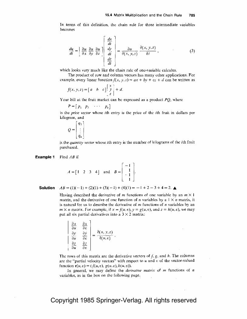
Copyright 1985 Springer-Verlag. All rights reserved
15.4 Matrix Multiplication and the Chain Rule 785
In terms of this definition, the chain rule for three intermediate variables becomes
dx dt
du = [ ~ au au ] dy dt ax ay az dt
dz dt
au a(x, y,z)
a(x, y,z) at
which looks very much like the chain rule of one-variable calculus.
(3)
The product of row and column vectors has many other applications. For example, every linear functionf(x, y,z) =ax+ by+ cz + d can be written as
f(x,y,z)=[a b c][;]+d.
Your bill at the fruit market can be expressed as a product PQ, where
P=[P1 P2 Pn] is the price vector whose ith entry is the price of the ith fruit in dollars per kilogram, and
qi
Q= qn
is the quantity vector whose ith entry is the number of kilograms of the ith fruit purchased.
Example 1 Find AB if
A ~ [ I 2 3 4 J and B ~ r = !] Solution AB= (l)(-1) + (2)(1) + (3)(-1) + (4)(1) = -1 + 2 - 3 + 4 = 2 . .&
Having described the derivative of m functions of one variable by an m X I matrix, and the derivative of one function of n variables by a 1 X n matrix, it is natural for us to describe the derivative of m functions of n variables by an m X n matrix. For example, if x = j(u,v),y = g(u,v), and z = h(u,v), we may put all six partial derivatives into a 3 X 2 matrix:
ax ax au av ay ay a(x, y,z)
au av a(u,v) az az au av
The rows of this matrix are the derivative vectors off, g, and h. The columns are the "partial velocity vectors" with respect to u and v of the vector-valued function r(u,v) = (j(u,v), g(u,v),h(u,v)).
In general, we may define the derivative matrix of m functions of n variables, as in the box on the following page.

Copyright 1985 Springer-Verlag. All rights reserved
786 Chapter 15 Partial Differentiation
Derivative Matrix Let u, = j,(x,,x2, ... 'xn), U2 = f2(x,,X2, ... 'xn), ... ' and um= f m ( x I' X2' ... ' xn) be m functions of the n variables x I' ... ' xn. The derivative matrix of the u;'s with respect to the x/s is the m X n matrix:
au, au, au, ax, ax2 axn
ac u,' ... ' um) au2 au2 au2 ax, ax2 axn
acx,, ... ,xn)
aum aum aum ax, ax2 axn
whose (i, j) entry is the partial derivative aujaxj.
The entries of the derivative matrix are functions of ( x 1, .•. , xn). If we fix values (x?, ... , x~) for the independent variables, then the derivative matrix becomes a matrix of numbers and is denoted by
acu,, .... um) I ac XI ' ... ' Xn) (x?, ... , x::J
Example 2 Let u = x 2 + y 2, v = x 2 - y 2, and w = xy. Find a(u, v, w)/a(x, y) and evaluate
acu,v,w) I acx, y) (-2,3)
Solution Applying the definition, with m = 3, n = 2, u1 = u, u2 = v, u3 = w, x 1 = x, and x2 = y, we get
acu,v,w) -[2x a(x, y) - 2x
y
Substituting x = - 2 and y = 3, we get
acu.v,w)I [-4 a(x,y) (-2,3)= -1 - ~ ]· .A.
-2
Notice that the derivative matrix of one function u = j(t) of one variable is a 1X1 matrix a(u)/a(t) whose single entry is just the ordinary derivative du/ dt. Thus the chain rule (3) can be rewritten as
a(u) a(u) acx, y,z) - - (4) a(t) acx, y,z) a(t)
In the remainder of this section, we will show how to multiply matrices of all sizes and, thereby, to generalize the chain rule (4) to several independent and dependent variables.

Copyright 1985 Springer-Verlag. All rights reserved
15.4 Matrix Multiplication and the Chain Rule 787
Example 3 (a) Suppose that u =ax+ by+ cz + d and v =ex+ fy + gz + h, where a, b, ... , h are constants.
(i) Express u and v by using products of row and column vectors. (ii) Find the derivative matrix 3(u,v)/3(x, y,z).
(b) Suppose that x, y, and z in (a) are linear functions oft:
x =mt+ n,y =pt+ q, and z =rt+ s.
(i) Express u and v in terms oft and find the derivative matrix a( u, v) I a( t). (ii) Express the elements of 3(u,v)/3(t) as products of row and column
vectors.
Solution (a) (i) We have u =[ab c][ ~] + d
andv=[efg][~] +h.
(ii) The derivative matrix is
3(u,v) [a b c] 3(x,y,z) = e J g '
all of whose entries are constants.
(b) (i) Substituting for x, y, and z their expressions int, we get
u = a(mt + n) + b(pt + q) + c(rt + s) + d,
v = e(mt + n) + f(pt + q) + g(rt + s) + h.
We can find the derivative matrix without multiplying out:
3(u,v) = r ~~ 1 =[am+ hp+ er]· 3( t) dv em + fp + gr
dt
(ii) The entries of 3(u,v)/3(t) are
Notice that they are obtained by multiplying the rdws of 3(u,v)/3(x,y,z) by the (single) column of a(x, y,z)/3(t) . ...
The preceding example and the multiplication of row and column vectors suggest how we should multiply m X n matrices.
Matrix Multiplication Let A and B be two matrices and assume that the number of columns of A equals the number of rows of B. To form C =AB:
1. Take the product of the first row of A and first column of B and let it be the (1, 1) entry of C.
2. Take the product of the first row and second column of B and let it be the (1, 2) entry of C.
3. Repeat. In general, the product of the ith row of A and jth column of B is the (i, j) entry of C.

Copyright 1985 Springer-Verlag. All rights reserved
788 Chapter 15 Partial Differentiation
Example 4 Let
Solution
- o1] -3
and B = [ i Find AB and BA.
[; ~.~·][i -~] =[ 1·2+(-'-l)·l 8 - 3 . H1 l
(going across the first row of A and down the first column of B ). Moving to the second column of B:
Moving to the second and third rows of A, we fill in the remaining entries:
= 4 0 . OJ [ 1. 1] - 1 13 3
BA is not defined since the number of columns of B is not equal to the number of rows of A. A.
Example 5 Find:
Solution
[ ; 6 ][ 6 iJ and [ 6 i ] [ ; 6 l [ ; 6 ] [ 6 n = [ ; ~ ] and [ 6 i ][ ; 6 ] = [ ~ 6 l ...
Example 5 shows that even if AB and BA are defined, they may not be equal. In other words, matrix multiplication is not commutative.
Example 6 For 2 X 2 matrices A and B, verify that IAB I= IA I IB I, where IA I denotes the determinant of A (Section 13.6).
Solution Let
A = [: ~] and B = [ ~ £l Then IA I= ad - be, IBI =eh - gf, and
IABI = lae + bg af + bhl ce + dg cf+ dh
= ( ae + bg)( cf+ dh) - ( ce + dg)( af + bh)
= aecf + aedh + bgcf + bgdh - aecf- adgf- cebh - bgdh
= aedh + bgcf - adgf - cebh
=(ad- be)( eh -gf)
=IAl·IBl.A.

Copyright 1985 Springer-Verlag. All rights reserved
15.4 Matrix Multiplication and the Chain Rule 789
The result of Example 3(b) may be written in the following way in terms of derivative matrices:
a(u,v) acu,v)
a(tf = a(x, y,z)
This suggests a similar formula for the general chain rule.
The General Chain Rule Let U1 = f1(X1, ... , xn), ... ' um= fm(Xi, ... , xn) be m functions of n variables, and let x 1 = g1(t1, ... , tk), ... , xn = gn(t1, ... , tk) be n functions of k variables, all with continuous partial derivatives.
Consider the u/s as functions of the 0's by
U1 = f1(g1(t1' · · ·' tk), · · ·, gn(tl' · · · 'tk)).
Then
ac U1' ... , um)
au l ' ... ' tk)
acu1' ... 'um) acx1, ... 'xn)
acx1,···•xn) au1,····tk).
In other words,
au; au; axl au; ax2 au; axn -=--+--+···+--. a0 axl a0 ax2 a0 axn a0
(Note that there are as many terms in the sum as there are intermediate variables.)
We will carry out the proof for the "typical" case m = 2, n = 3, k = 2. We must prove that
axl axl
1~ ~1 au] au]
~1 at1 at2
at1 at2 axl ax2 ax3 ax2 ax2
au2 au2 au2 au2 au2 at1 at2 at1 a12 axl ax2 ax3 ax3 ax3
at1 at2
This matrix equation represents four ordinary equations. We will prove a typical one:
au2 au2 ax] au2 ax2 au2 ax3 -=--+--+-- (5) at] axl ati ax2 atl ax3 at] .
In taking the partial derivatives with respect to t 1, we hold t2 fixed and take ordinary derivatives with respect to t 1. With this understood, we may rewrite (5) as
(6)
We are now in the situation of Section 15.3-we have the independent variable t1, the dependent variable u2 , and intermediate variables (x 1,x2,x3); but the chain rule for this case is just formula (6), so (6) is true and hence (5) is proved.

Copyright 1985 Springer-Verlag. All rights reserved
790 Chapter 15 Partial Differentiation
Example 7 Verify the chain rule for op/ox, where
p=f(u,v,w)=u2+v2-w, u=xy, v=y2, and w=e-xz.
Solution j(u,v, w) = (xy)2 + y 4 - e-xz = xy2 + y 4
- e-xz. Thus
~~ = 4xy2 + ze-xz.
Example 8
Solution
On the other hand,
a · a a J!... au + J!... av + _J!_ aw = 2u(2xy) + 2v. 0 + ze-xz au ax av ax aw ax
= (2xy)(2xy) + ze-xz,
which is the same . .&
Let (x, y) be cartesian coordinates in the plane and let (r,O) be polar coordinates. (a) If z = j(x, y) is a function on the plane, express the partial derivatives oz/or and oz/aO in terms of oz/ax and oz/oy. (b) Express o2z I a r2 in Cartesian coordinates.
(a) By the general chain rule, using x = r cos 0 and y = r sin 0,
[ az ar
r
ax
az J Tr ay ay
ar
oz ] [ cosO ay sin(}
Multiplying out,
az = k cosO + az sinO ar ax ay '
az = r[- k sin(}+ ~ coso]. ao ax ay
(b) By (a),
az = k cosO + az sinO. ar ax ay
ax j ao ay ao
-rsinOJ· rcosO
(7)
Thus 02
z = l_ [ k JcosO + l_ [ oz JsinO. Applying equation (7) with a,2 ar ax ar ay oz/ax and az/ay replacing z, we get
02~ = ( 02
z2 cosO + 0°2
0z sinO)cosO + ( 0°2
z0
cosO + 02
z sinO)sinO ar ax y x x y ay2
= 02z cos20 + 2 ~ sin(} cos(} +
02z sin20 ax2 ay ax ay 2
= 1 [ x2 a2z + 2xy ~ + y2 o
2z ] . .&
x2 + y2 ax2 ax ay ay2
Example 9 Suppose that (t,s) = (j(x, y), g(x, y)), x = u - 2v, and y = u + 3v. Express the derivative matrix o(t,s)/o(u,v) in terms of o(t,s)/o(x,y).
Solution By the chain rule,
o(t,s) - o(t,s) o(x, y) o(u,v) - o(x, y) o(u,v) .

Copyright 1985 Springer-Verlag. All rights reserved
In this example,
a(x,y)=[l a(u,v) 1
so
- 2] 3 '
a(t,s) = a(t,s) [ 1 a(u,v) a(x,y) 1
Exercises for Section 15.4 Find the matrix products in Exercises 1-4.
1. [l 2 3][ i l 1 2
4. [l 2 3
Find the derivative matrices in Exercises 5-8 and evaluate at the given points.
5. a(x, y)/a(u, v); x = u sin v, y = euv; at (0, 1). 6. a(x, y, z)/a(r, 0, </>); where x = r sin</> cos 0,
y = rsin<t>sinO, z = rcoscp; at (2,w/3,w/4). 7. a(u,v)/a(x, y,z); u = xyz, v = x + y + z;
at (3, 3, 3). 8. a(x, y)/a(r, O); x = r cos 0, y = r sin O; at (5, w /6).
Compute the matrix products in Exercises 9-20 or explain why they are not defined.
9. [6 7][~ ~] 10. [6 ~J[~ n 11. [~ 6][~ ~] 12. [6 n[~ ~J 13. [~ jJ[i] 14. [i][i] 15. [~ n[~J 16. [ i : j[~ 0
2
[6 ~][~ ~] 18. [ g 0
rn~ 17. 1 0
19. (U ~JU -iD[6 !J 20
· u ~ ] ( u -i ] [ 6 ~ ])
15.4 Matrix Multiplication and the Chain Rule 791
r
at
-n = ~: ax
at 1 ay [I as 1 ay
-21!..+31f.1 ax ay •• -2k +3~ ax ay
Compute az/ax and az/ay in Exercises 21-24 using matrix multiplication and by direct substitution.
21. z = u2 + v 2; u = 2x + 7, v = 3x + y + 7.
22. z = u2 + 3uv - v 2; u = sinx, v= -cosx+cosy.
23. z = sinucosv; u = 3x2 - 2y, v = x - 3y.
24. z = u/v2; u = x + y, v = xy.
25. (a) Compute derivative matrices a(x, y)/a(t, s) and a(u,v)/a(x, y) if
x = t + s, y = t - s,
u = x2 + y2, v = x2 - y2.
(b) Express ( u, ti) in terms of (t, s) and calculate a(u,v)/a(t,s).
(c) Verify that the chain rule holds. 26. Do as in Exercise 25 for the functions
x = t 2 - s2
, y = ts, u = sin(x + y), v = cos(x - y).
27. Do as in Exercise 25 for x = ts, y = ts; u = x, v= -y.
28. Do as in Exercise 25 for x = t2 + s2, y = t2 - s2,
z = 2ts; u = xy, v = xz, w = xz.
29. Suppose that a function is given in terms of rectangular coordinates by u = f(x, y,z). If
x = r cos 0 sin </>,
y = r sin 0 sin </>,
z = rcoscp,
express au/ar, au;ao, and au/acp in terms of au/ax, au/ay, and au;az.
30. Suppose that x, y,z are as in Exercise 29 and u = x 2 + y 2 + z 2
• Find au/ar, au/aO, and au/aq,.
31. Express the polar coordinates r and 0 in terms of the cartesian coordinates x and y, and find the derivative matrix a(r, O)/a(x, y).

Copyright 1985 Springer-Verlag. All rights reserved
792 Chapter 15 Partial Differentiation
32. Let A be the derivative matrix a(x, y)/a(r, (})for x = r cos(}, y = r sine. Let B be the derivative matrix a(r, {})ja(x, y) of Exercise 31, with its entries expressed in terms of r and (}. Find AB and BA.
33. Let B be the m x 1 column vector
m
m
m
If A = [a1 • • • aml is any row vector, what is AB? Exercises 34-38 form a unit.
34. Let
I = [ b n and A = [ b i]. Find a matrix B such that AB = I.
35. In Exercise 34, show that we also have
BA= [ b ~l 36. Show that the solution of the equation
where A and B are as in Exercises 34 and 35. 37. Find a matrix B such that
B[~ ~]=[6 ~l 38. Using the results of Exercises 36 and 37, solve
each of the following systems of equations: (a) x + 2y = 1, 2x + 5y = 2; (b) x + 2y = 0, 2x + 5y = 0.
Exercises 39-42 form a unit. 39. If (f1(x 1, ... , xn), ... , fn(X1, ... , xn))
= ( u1, ••• , un) are n functions of n variables, then the (square) matrix of partial derivatives is called the Jacobian matrix. Its determinant is called the Jacobian determinant and is denoted by
I a( U I , · · · , Un) I · a(x1, ... , xn)
(a) Suppose that n = 2. Show that the absolute value of
I a(u 1 ,u2) I I a(x, y) (a,b)
is the area of the parallelogram spanned by
( au
1 I au2 I ) ax (a,bi' ax (a,b)
and
( au1 I au
2 ' ) aJ (a,bi' Ty (a,b) .
(b) Suppose that n = 3. Show that the absolute value of
I a(u 1 ,u2 ,u3) I I a( XI 'X2 'X3) (a,b,c)
is the volume of the parallelepiped spanned by the vectors
( au1 I au2 I au3 / ) h 'h 'h 1 (a,b,c) 1 (a,b,c) 1 (a,b,c)
for i = 1,2,3. 40. Compute the following jacobian determinants:
(a) (x, y) = (r cos(}, r sin(}). Find
I a(x,y) /· a(r, (})
(b) Let (x, y,z) = (rcose,rsin(},z). Find
I a(x,y,z) /· a(r, (}, z)
(c) Let (x, y, z) = (r cos(} sin <j>, r sin(} sin <j>, rcostj Find
I a(x,y,z) /· a(r, (}, </>)
41. Compute the jacobian determinants (see Exercise 39) of the following functions at the indicated points: (a) (x, y) = (t 2 + s2
, t2 - s2
); (t,s) = (1,2). (b) (u,v) = (x + y,xy); (x, y) = (5, -3). ( c) Compute the jacobian determinant of ( u, v)
with respect to (t,s) from parts (a) and (b) at (t,s) = (1,2). Verify that your answer is the product of the answers in (a) and (b).
42. Prove the following equations (notation from Exercise 39) in light of the chain rule and the multiplicative property of determinants found in Example 6:
(a) I
~ 11 a( x, y) I = I a( u, v) 1 · a(x, y) a(t,s) a(t,s) ,
(b) I a(x, y) II a(t,s) I= 1. a(t,s) a(x, y)
43. Let v 1 , v2, v3 be the components of a vector function v, u a scalar function, a, b, p constants. Express in matrix notation the equations of elasticity:
p( a2v:) =(a+ b)( aau) + b( a
2v3 + a
2v3 + a
2v3 )·
at z ax 2 ay 2 az 2

Copyright 1985 Springer-Verlag. All rights reserved
44.
45.
46.
A rotation of points in the xy plane (relative to fixed axes) is given by
[XJ = [cos8 y S!Il 8
-sin8][x] cos8 y
where 0 is the angle of rotation of
[;] into [ ~] Show by means of matrix multiplication that a rotation of 81 followed by a rotation of 82 is the same as a rotation of 82 followed by a rotation of 81. The coordinates u, r:p, 8 are defined by x = au sin r:p cos 8, y = bu sin r:p sin 8, z = cu cos r:p for u > 0, 0 < r:p < 7T, 0 < 8 < 27T. (a) Show that the surfaces u = constant are the
ellipsoids
( :J 2
+ (tu f + ( :u f =I.
(b) Show that the surfaces r:p =constant are elliptical cones.
(c) Show the surface 8 =constant is a plane. ( d) Volume calculations involve the determi
nant of a(x, y, z)/a(u, r:p, 8). Show that it equals !]bcu2sin r:p.
The matrix equation
[X] [cos8 ~ = si~B
can be viewed as a rotation in the xy plane through the angle 0. (See Exercise 4.4). Similarly, the equation
can be viewed as a translation in the xy plane. (a) Use a matrix multiplication to find the ma
trix equation for a rotation followed by a translation.
(b) Is a rotation followed by a translation the same as a translation followed by a rotation?
Review Exercises for Chapter 15 Calculate all first partial derivatives for the functions in Exercises 1-10.
sin( 7TX) I. u = g(x, y) = --- .
I+ y2 2. u = f(x, z) = __ :X __ .
1 + cos(2z) 3. u = k(x, z) = xz2 - cos(xz 3).
4. u = m(y,z) = yz.
5. u = h(x, y,z) = zx + y 2 + yz. 6. u = n(x, y,z) = xYz. 7. u = f(x, y,z) =In[!+ e-'cos(xy)]. 8. u = h(x, y,z) = cos(e-x'- 2Y').
Review Exercises for Chapter 15 793
*47. Verify the formula IABI = IAI IBI for 3 X 3 matrices A and B, where IA I denotes the determinant of A.
*48. Public health officials have located four persons, x 1 , x 2 , x 3 , and x4 , known to be carrying a new strain of flu. Three persons, y 1, Ji, and y 3 , report possible contact, and a first-order contact matrix A is set up whose i, )th entry is I if there was contact between X; and y1 and zero otherwise. Five other people, z 1, z 2 , z3 , z 4 , and z5 , are questioned for possible contact with y 1, Ji, and y 3 , and another first-order contact matrix Bis set up whose i, jth entry is 1 if y; has contacted z1 and zero otherwise. (a) Show that the product matrix C =AB
counts the number of second-order contacts. That is, the i,jth entry of C is the number of possible paths of disease communication from X; to z1 .
(b) Write down the three matrices for the situation shown in Fig. 15.4.2. Check the conclusion of part (a).
Figure 15.4.2. Contacts between three groups of people.
*49. Express Simpson's rule (Section 11.5) by using a product of row and column vectors.
*50. Suppose that f is a differentiable function of one variable and that a function u = g(x, y) is defined by
u = g(x,y) = xyf( x ~y )·
Show that u satisfies a (partial) differential equation of the form
2 au 2 au ( ) x - - y - = G x, y u ax ay
and find the function G(x, y).
9. u = g(x, y, z) = xz + e 2 (foxt 2e' dt).
10. u = j(x, y) = cos(xy2) +exp[ fax It cos( ty) dt l
Check the equality of the given mixed partials for the indicated functions in Exercises 11-16.
11. a2u/ax ay = a2u/ay ax for u in Exercise I. 12. a2u/ax az = a2u/az ax for u in Exercise 2. 13. a2u/ax az = a2u/az ilx for u in Exercise 3. 14. a1u/ay az = a2u/az ay for u in Exercise 4.
15. a2u/ax az = a2u/az ax for u in Exercise 5. 16. a2u/ax az = a2u/az ax for u in Exercise 6.

Copyright 1985 Springer-Verlag. All rights reserved
794 Chapter 15 Partial Differentiation
17. Find (a /ax)ex-cos(yx) Ix~ I,ro·
18. Find (a/as)exp(rs3 - r3s)l,~i,s~I·
19. Find fx(l, 0) if f(x, y) = cos(x + eyx).
20. Find fs(-1, 2) if f(r,s) = (r + s 2)/(1 - r2 - s2
).
21. The possible time T in minutes of a scuba dive is given by T = 32 V /(x + 32), where Vis the volume of air in cubic feet at 15 psi (pounds per square inch) which is compressed into the air tanks, and x is the depth of the scuba dive in feet. (a) How long can a 27-foot dive last when
V= 65? (b) Find aT/ax and ar/av when x=27,
V = 65. Interpret. 22. The displacement of a certain violin string placed
on the x axis is given by u = sin(x - 6t) + sin(x + 6t). Calculate the velocity of the string at x = 1 when t = t.
Find the limits in Exercises 23-26, if they exist.
23.
24.
25.
26.
Jim (x 2 - 2xy + 4) (x,y)->(0,0)
Jim (x 3 - y 3 + 15) ( x .y )->(0,0) 3 3
Jim x - y (x,y)->(0,0) x2 + Y2
Jim xy + x 3 + x - 2
(x,y)->(0,0) -Jx2 + Y2
Find the equation of the tangent plane to the given surface at the indicated point in Exercises 27-30.
27. z = x 2 + y 2; x = I, y = 1.
28. z = x sin y; x = 2, y ='IT /4. 29. Z = eXY; X = 0, Y = 0.
30. z = -/x 2 + y 2 ; x = 3, y = 4.
Use the linear approximation to find approximations for the quantities in Exercises 31-34.
31. VCI.01)2 + (4.01)2 + (8.002)2
32. (2.004)ln(0.98) 33. (0.999)1.00l 34. (1.001)0.999
35. Find an approximate value for the hypotenuse of a right triangle whose legs are 3.98 and 3.03.
36. The capacitance per unit length of a parallel pair of wires of radii R and axis-to-axis separation D is given by
The capacitance between a wire and a plane parallel to it is
2m•0 C* = --------
( h + i/h 2
- R 2
) In R
where h = distance from the wire to the plane.
(a) Find the expected change in capacitance for two parallel wires, separated by 2 centimeters, with radius 0.40 centimeter, due to a radius increase of 0.01 centimeter.
(b) A wire of 0.57 centimeter radius has its central axis at a uniform distance of 3 centimeters from a conducting plane. Due to heating, the wire increases 0.02 centimeter in radius, but due to bowing of the wire, it can be assumed that the axis of the wire was raised to 3.15 centimeters above the plane. What is the expected change in capacitance?
37. At time t = 0, a particle is ejected from the surface x 2 + 2y2 + 3z2 = 6 at the point (1, 1, 1) in a direction normal to the surface at a speed of 10 units per second. At what time does it cross the sphere x 2 + y 2 + z 2 = 103? [Hint: Solve for z].
38. At what point(s) on the surface in Exercise 37 is the normal vector parallel to the line x = y = z?
39. Verify the chain rule for the function f(x, y, z) = ln(l + x 2 + 2z 2)/(1 + y 2
) and the curve u(t) = (t, 1 - t 2
, cost). 40. Verify the chain rule for the function f(x, y)
= x 2 /(2 +cosy) and the curve x = e', y = e-'. 41. (a) Let c be a constant. Show that, for every
function f(x), the function u(x, t) = f(x - ct)
satisfies the partial differential equation u, + cux = 0.
(b) With u as in (a), consider for each value oft the graph z = u(x, t) in the xz plane. How does this change as t increases?
42. (a) Show that, if u(x, t) is any solution of the equation u, + cux = 0, then the function g(y, t)
defined by g(y, t) = u(y + ct, t) is independent oft.
(b) Conclude from (a) that u must be of the form u(x, t) = f(x - ct) for some function f.
(c) What kind of wave motion is described by the equation u, + cux = O?
43. A right circular cone of sand is gradually collapsing. At a certain moment, the cone has a height of 10 meters and a base radius of 3 meters. If the height of the cone is decreasing at a rate of 1 meter per hour, how is the radius changing, assuming that the volume remains constant?
44. A boat is sailing northeast at 20 kilometers per hour. Assuming that the temperature drops at a rate of 0.2°C per kilometer in the northerly direction and 0.3°C per kilometer in the easterly direction, what is the time rate of change of temperature as observed on the boat?
45. Use the chain rule to find a formula for (d/ dt)exp(j(t)g(t)].
46. Use the chain rule to find a formula for ( d / dt)(f( t)g(I) ).

Copyright 1985 Springer-Verlag. All rights reserved
47. If x and y are functions oft,
dx I = I, and dy I = - I, dt r~o dt i~o
find !:!_ ex+lxyl in terms of x and y. dt 1~0
48. If x, y, and z are functions of t and
dxl =I dyl -0 dt i~o , dt r~o
and dz I = - I find dd cos(xyz2)1 in dt 1~0 , t 1~0
terms of x, y, and z. 49. The tangent plane to z = x 2 + 6y2 at x = I, y = 1
meets the xy plane in a line. Find the equation of this line.
50. The tangent plane to z = ex-y at x = 1, y = 2 meets the line x = t, y = 2t - 1, z = 5t in a point. Find it.
Find the products AB of the matrices in Exercises 51-60.
51. A =[I 2 4], B = [ - : l 52 A -[ t i ± HB-l;l;J 53 A= [ O . 1
54. A= u 55. A= u
-6JB=[6 -n n' B = [ - ~ ! ] ~Js=[; =~J
56. A = rn = ~ J B = u ~ ] 57. A = [ - ~ n, B = [ _; _ ~ n SSA - [ : ~ i : i'o l B -l = j 1 59. A= [I 0
-}}B=[i 0 -) l 2 0 0 I
60. A= [ i 0 - I] [ 3 0 -~ l 0 b , B = ! 2 1 0
61. Compute az/ax and az/ay if
u2 + v2 u = e-x-y, v = exy z=---u2 - v2 '
by (a) substitution and (b) the chain rule. 62. Do as in Exercise 61 if z = uv, u = x + y, and
v = x -y. 63. Suppose that z = f(x, y), x = u + v and y = u-v.
Express az /au and az /av in terms of az /ax and az/ay.
Review Exercises for Chapter 15 795
64. In the situation of Exercise 63, express az/ax and az/ay in terms of az/au and az/av.
65. The ideal gas law PV = nRT involves a constant R, the number n of moles of the gas, the volume V, the Kelvin temperature T, and the pressure P.
(a) Show that each of n,P, T, Vis a function of the remaining variables, and determine explicitly the defining equations.
(b) The quantity ap /a T is a rate of change. Discuss this in detail, and illustrate with an example which identifies the variables held constant.
(c) Calculate a V /aT, aT /aP, aP /a V and show that their product equals - I.
66. The potential temperature B is defined in terms of temperature T and pressure p by
( 1000 )0.286
B=T - . p
The temperature and pressure may be thought of as functions of position (x,y,z) in the atmosphere and also of time t. (a) Find formulas for ao /ax, ao jay, ao /az,
ao /at in terms of partial derivatives of T andp.
(b) The condition ao /az < 0 is regarded as unstable atmosphere, for it leads to large vertical excursions of air parcels from a single upward or downward impetus. Meteorologists use the formula
ao=!J.._(aT+JL) az T az CP '
where g = 32.2. CP = constant > 0. How does the temperature change in the upward direction for an unstable atmosphere?
67. The specific volume V, pressure P, and temperature T of a Van der Waals gas are related by P =[RT/( V - ,B)] - a/ V 2, where a, {3, R are considered to be constants. (a) Explain why any two of V, P, or T can be
considered independent variables which determine the third variable.
(b) Find a T /aP, aP ;av, av ;a T. Identify which variables are constant, and interpret each partial derivative physically.
(c) Verify that (a T /aP)(aP ;a V)(a v ;a T) =
-1(not+1!). 68. Dieterici's equation of state for a gas is
P( V - b)ea/RVT =RT,
where a, b, and R are constants. Regard volume V as a function of temperature T and pressure P and show that

Copyright 1985 Springer-Verlag. All rights reserved
796 Chapter 15 Partial Differentiation
69. What is wrong with the following argument? Suppose that w = f(x, y) and y = x 2. By the chain rule,
aw = aw ax + aw ay = aw + 2x aw . ax ax ax ay ax ax ay
Hence 0 = 2x(aw /ay), so aw jay= 0. 70. What is wrong with the following argument?
Suppose that w = f(x, y,z) and z = g(x, y). Then by the chain rule,
aw = aw ax + aw ay + aw ~ ax ax ax ay ax az ax
- aw+ aw az - ax a; ax.
Hence
0 = aw az az ax,
so aw /az = 0 or az /ax = 0, which is, in general, absurd.
71. For a function u of three variables (x, y,z), show that a3u/ax ay az = a3u/ay az ax.
72. For a function u of three variables (x, y, z), show that a3u/ax ay az = a3u/az ax ay.
73. Prove that the functions (a) f(x, y) = ln(x2 + y 2
),
1 (b) g(x, y,z) = 1;2'
(x2 + y2 + z2) 1 (c) h(x,y,z,w)= 2 2 2 2 ,
x+y+z+w satisfy the respective Laplace equations: (a) fxx + /yy = 0, (b) gxx + gyy + gzz = 0, (c) hxx + hyy + hzz + hww = 0,
where !xx = a2f /ax2, etc. 74. If z = f(x - y)/y, show that
z + y(az/ax) + y(az/ay) = o.
75. Given w = f(x, y) with x = u + v, y = u - v, show that
a2w a2w a2w au av - ax2 ay2
*76. (a) A function u = f(x 1, ... , xm) is called homogeneous of degree n if
J(tx 1, ... , txm) = t"f(x1, ... , xm).
Show that such a function satisfies Euler's differential equation
au au au - if( ) x 1 - +x2- + · · · + Xm-- - n X1, ... , Xm. ax! ax2 axm
(b) Show that each of the following functions satisfies a differential equation of the type in part (a), find n, and check directly that f is homogeneous of degree n.
(i) f(x, y) = x 2 + xy + y 2;
(ii) f(x,y,z) = x + 3y-{Xi; xz > O; (iii) f(x, y, z) = xyz + x 3
- xy. * 77. In Exercise 77 on page 775 we saw that the
mixed partial derivatives of
z=
xy(x2 - y2) z=
x2 + y2
at (0, 0) are not equal. Is this consistent with the graph in Fig. 15.R.l?
x2 + y2

Copyright 1985 Springer-Verlag. All rights reserved
Chapter16
Gradients, Maxima, and Minima
The gradient of a Junction of several variables vanishes at a maximum or a minimum.
The gradient of a function f is a vector whose components are the partial derivatives of f. Derivatives in any direction can be found in terms of the gradient, using the chain rule. The gradient will be used to find the equations for tangent planes to level surfaces. The last two sections of the chapter extend our earlier studies of maxima and minima (Chapter 3) to functions of several variables.
16.1 Gradients and Directional Derivatives The directional derivative is the dot product of the gradient and the direction vector.
The right-hand side of the chain rule
du = ~ dx + au dy + au dz dt ax dt ay dt az dt
has the appearance of a dot product-in fact it is the dot product of the vectors
dx i + dy . + dz k and dt dt J dt
We recognize the first vector as the velocity vector of a parametric curve; if u(t) is the vector representation of the curve, it is just u'(t). The second vector is something new: it depends upon the function u = j( x, y, z) and contains in vector form all three partial derivatives off. This is called the gradient off and is denoted V f. Thus
VJ(x, y,z) = fx(x, y,z)i + fy(x, y,z)j + fz(x, y,z)k.
Example 1 (a) Find VJ if u = j(x,y,z) = xy- z 2•
(b) Find Vf for the functionj(x,y,z) = exy _ xcos(yz 2).
Solution (a) Substituting the partial derivatives off into the formula for the gradient of f, we find V j(x, y, z) = yi + xj - 2zk.

Copyright 1985 Springer-Verlag. All rights reserved
798 Chapter 16 Gradients, Maxima, and Minima
(b) Here fx(x, y,z) = yexy--, cos(yz 2), fy(x, y,z) = xexy + xz2sin(yz 2
), and .fz(x, y, z) = 2xyz sin(yz 2
), so
V f( x, y, z) = [ yexy - cos(yz2) Ji + [ xexy + xz 2sin(yz2
) )j
+ [ 2xyz sin(yz2) Jk. •
Notice that the vector Vf(x,y,z) is a function of the point (x,y,z) in space; in other words, V f is a function of the point in space where the partial derivatives are evaluated. A rule «I> which assigns a vector <l>(x, y,z) in space to each point (x, y, z) of some domain in space is called a vector field. Thus, for a given function f, V f is a vector field. Similarly, a vector field in the xy plane is a rule «I> which assigns to each point (x, y) a vector «l>(x, y) in the plane.
The Gradient If z = j(x, y) is a function of two variables, its gradient vector field V f is defined by
Vf(x,y)=fx(x,y)i+fy(x,y)j= ~~i+ ~;j.
If u = f(x, y,z) is a function of three variables, its gradient vector field V f is defined by
Vf(x, y,z) = fx(x, y,z)i + fy(x, y,z)j + .fz(x, y,z)k
= ~ i + au j + auk. ax ay az
We may sketch a vector field «l>(x, y) in the plane by choosing several values for (x, y), evaluating «l>(x, y) at each point, and drawing the vector «l>(x, y) with its tail at the point (x, y). The same thing may be done for vector fields in space, although they are more difficult to visualize.
Example 2 Sketch the gradient vector field of the function j( x, y) = x 2/10 + y 2 / 6.
Solution The partial derivatives are fx(x, y) = x /5 and fy(x, y) = y /3. Evaluating these for various values of x and y and plotting, we obtain the sketch in Fig. 16.1.1. For instance,fx(2,2) = ~ andfy(2,2) = 1; thus the vector ~i + 1j is plotted at the point (2, 2), as indicated in the figure . .6. ·
Figure 16.1.1. The gradient vector field V f, where j(x, y) = (x 2 /10) + (y 2 /6).
///
/II
y
x
~ '\"' \\\

Copyright 1985 Springer-Verlag. All rights reserved
16.1 Gradients and Directional Derivatives 799
In sketching a vector field «l>(x, y), we sometimes find that the vectors are so long that they overlap one another, making the drawing confusing. In this case, it is better to sketch e«l>(x, y), where e is a small positive number. This is illustrated in the next example.
Example 3 (a) Illustrate the vector field «l>(x, y) = 3yi - 3xj by sketching -l;-«l>(x, y). (b) Using the law of equality of mixed partial derivatives, show that the vector field in (a) is not the gradient vector field of any function.
Solution (a) If we sketched «l>(x, y) = 3yi - 3xj itself, the vectors at different base points would overlap. Instead we sketch -l;-«l>(x, y) = iyi -1 xj in Fig. 16.1.2.
Figure 16.1.2. The vector field 3yi - 3xj is not the gradient of a function.
y
x
(b) If «l>(x, y) = 3yi - 3xj were the gradient of a function z = j(x, y), we would have az/ax = 3y and az/ay = -3x. By the equality of mixed partial derivatives, a2z ;ax ay = - 3 and a2z jay ax = 3 would have to be equal; but 3 =I= - 3, so our vector field cannot be a gradient. .A.
In a number of situations later in the book, the vector r from the origin to a point (x, y, z) plays a basic role. The next example illustrates its use.
Example 4 Let r = xi+ yj + zk and r = llrll = ~x2 + y 2 + z2• Show that
v( l) = - _!_ , r r3
r =I= 0.
What is llV(l/r)ll? Solution By definition of the gradient,
v( l) = __l_ ( 1 )i + __l_ ( l )j + JL. ( l )k. r ax r ay r az r
Now
aax u) ~ a°x ( ~x' + ~' + z' ) ~ - ( x' + y: + z')'i' ~ - ;, , and, similarly,
J!...(l)=-L ay r r3 ' JL.(l)=-.!.... az r r3 .
Thus
V( I ) x . Y . z k 1 ( . + . + k) r - = - - I - - J - - = - - XI YJ z = - - ' r r3 r3 r3 r3 r3

Copyright 1985 Springer-Verlag. All rights reserved
800 Chapter 16 Gradients, Maxima, and Minima
as required. Finally,
V - = - - \Ir\\ = - = - = A II ( 1 ) II I 1 I r 1 1 r r3 r3 r2 x2 + y2 + z2 ·
In the next box we restate the chain rule from Section 15.3 m terms of gradients.
The Chain Rule for Functions and Curves Let f be a function of two (three) variables, u(t) a parametric curve in the plane (in space), and h(t) = j(u(t)) the composite function. Then
h'( t) = V f( u( t)) · u'( t); that is, fr J( u( t)) =VJ( u( t)) · u'(t).
In this form, the chain rule looks more like it did for functions of one variable:
fr (f(g(t))) = f'(g(t))g'(t).
Example 5 Verify the chain rule for u = j(x,y,z) = xy- z 2 and u(t) = (sint,cost,e 1).
Solution The gradient vector field off is yi + xj - 2zk; the velocity vector is given by u'(t) =cos ti - sin tj + e 1k. By the chain rule,
~~ = V f · u' = (yi + xj - 2zk) • (cos ti - sin tj + e 1k)
= ycost - xsint - 2ze 1 = cos2t- sin2t - 2e21 .
To verify this directly, we first compute the composition as j( u(t)) = sin t cost - e21. Then by one-variable calculus, we find
fr f(u(t)) = -sin2t + cos2t - 2e21 .
Thus the chain rule is verified in this case. A
Example 6 Suppose that f takes the value 2 at all points on a curve u(t). What can you say about Vf(u(t)) and u'(t)?
Solution If f(u(t)) is always equal to 2, the derivative (d/ dt) j(u(t)) is zero. By the chain rule, 0 = V j( u(t)) · u'( t), so the gradient vector V f( u( t)) and the velocity vector u'(t) are perpendicular at all points on the curve. A
Let u = j(x, y,z) be a function (with continuous partial derivatives) and u(t) a parametrized curve in space. The derivative with respect to t of the composite function j(u(t)) may be thought of as "the derivative off along the curve u(t)." According to the chain rule, the value of this derivative at t = t0 is V j( u(t0)) • u'(t0). We may write this dot product as
\\VJ(u(t0))11 llu'(t0)llcos0,
where 0 is the angle between the gradient vector V j( u(t0)) and the velocity vector u'(t0) (Fig. 16.1.3). If we fix the function f and differentiate it along various curves through a given point r (here, as usual, we identify a point with the vector from the origin to the point), the derivative will be proportional to the speed llu'(t0)11 and to the cosine of the angle between the gradient and

Copyright 1985 Springer-Verlag. All rights reserved
\1 f(u(t))
e a' (t)
x
Figure 16.1.3. The derivative off along the curve u( t) is
j_ f(u(t))=Vf(u(t)) · u'(t) dt = llVJ(u(t))ll llu'(t)llcosO.
16.1 Gradients and Directional Derivatives 801
velocity vectors. To describe how the derivative off varies as we change the direction of the curve along which it is differentiated, we fix r and choose u(t) = r + td ford a unit vector. (Note that since d is a unit vector, the speed of the curve u(t) is 1, so 1 unit of time corresponds to 1 unit of distance along the curve.)
We make the following definition: Let j(x, y, z) be a function of three variables, r a point in its domain, and d a unit vector. Define the parametric curve u(t) by u(t)=r+ td. The derivative (d/dt)j(u(t))l 1 = 0 is called the directional derivative off at r in the direction of d.
Since u'(t) = d and lldll = 1, we see that if f has continuous partial derivatives, the directional derivative at r in the direction of d is
V f(r) · d = II V f(r)llcos 0.
Notice that the directional derivatives in the directions of i, j, and k are just the partial derivatives. For instance, choosing d = i, V f · i = (j) + J;J + fzk) · i = fx. Similarly, V f · j = fy and V f · k = fz.
As we let d vary, the directional derivative takes its maximum value when cos 0 = 1, that is, when d points in the direction of V j(r). The maximum value of the directional derivative is just the length II V f(r)ll ·
The following box summarizes our findings.
Gradients and Directional Derivatives The directional derivative at r in the direction of a unit vector d is the rate of change off along the straight line through r in direction d; i.e., along u(t) = r + td.
The directional derivative at r in the direction d equals V j(r) · d. It is greatest (for fixed r) when d points in the direction of the gradient V j(r) and least when d points in the same direction as - V f(r).
Example 7 Compute the directional derivatives of the following functions at the indicated points in the given directions.
(a) j(x, y) = x + 2x2 - 3xy; (x0 , y 0) = (1, l); d = ( ~,v.
(b) j(x, y) = ln(~x 2 + y 2 ); (x0 , y 0) =(I, O); d = (2/5 /5,/5 /5).
(c) j(x, y,z) = xyz; (x0 , y 0 ,z0) = (1, 1, l); d = (l/ft)i + (l/ft)k. (d) f(x, y,z) =ex+ yz; (xo, Yo,Zo) = (1, 1, l); d = (1 I D)(i - j + k).
Solution (a) Vf(x,y)=(1+4x-3y,-3x). At (1,1) this is equal to (2,-3). The directional derivative is V j( x 0 , y 0) • d = (2, - 3) · ( ~, ~) = - ~.
(b) Vf(x,y) = (x/(x 2 + y 2),y/(x2 + y 2)), so Vf(l,O) = (1,0). Thus, the direc
tional derivative in direction (2/5 /5,/5 /5) is 2/5 /5. (c) Vf(x, y,z) = (yz,xz,xy), which equals (1, 1, 1) at (l, 1, 1). Ford equal to
(1/v'2,0, 1 / v'2 ), the directional derivative is 1 / v'2 + 0 + 1 / v'2 = v'2. (d) Vf(x,y,z) = (ex,z,y), which equals (e, I, 1) at (1, 1, 1). Ford equal to
(1 / Y3) · (i - j + k), the directional derivative is e(l / Y3) + 1 ( - 1 Y3) +
1(1/$) = e/$ . .A
If one wishes to move from r = ( x, y, z) in a direction in which f is increasing most quickly, one should move in the direction V j(r). This is because Vf(r) · d = llVf(r)llcosO is maximum when 0 = 0, i.e., cosO = 1, sod is in the direction of V j(r). Likewise, - V j(r) is the direction in which f is decreasing at the fastest rate.

Copyright 1985 Springer-Verlag. All rights reserved
802 Chapter 16 Gradients, Maxima, and Minima
Examples Let u=j(x,y,z)=(sinxy)e-z2
• In what direction from (1,'7T,0) should one proceed to increase f most rapidly?
Solution We compute the gradient:
VJ= aui+ auj+~k ax ay az
= y cos( xy)e-z2i + x cos ( xy)e-z
2j + ( -2z sinxy)e-z
2k.
At (1, '7T, 0) this becomes
'7T cos( '7T)i +cos( 'IT)j = - 'ITi - j.
Thus one should proceed in the direction of the vector - 'ITi - j. A.
Example 9 Captain Astro is drifting in space near the sunny side of Mercury and notices that the hull of her ship is beginning to melt. The temperature in her vicinity is given by T = e-x + e- 2
y + e3z. If she is at (1, 1, 1), in what direction should she proceed in order to cool fastest?
Solution In order to cool the fastest, the captain should proceed in the direction in which T is decreasing the fastest; that is, in the direction - V T(l, 1, 1). However,
Figure 16.1.4. The slope at the point P of the curve C in the plane 9 is the directional derivative at (x0 , y 0) off in the direction d.
VT - ar.+ ar.+ ark_ -x• 2 -2r+3 3zk - -1 -J - - -e 1- e J e . ax ay az
Thus,
-VT(l, 1, 1) = e- 1i + 2e- 2j - 3e3k
is the direction required. A.
Directional derivatives are also defined for functions of two variables. In this case, we have a geometric interpretation of the directional derivatives of j(x, y) in terms of the graph z = j(x, y). Given a point (x0 , y 0) in the plane and a unit vector d = ai + bj, we can intersect the graph with the plane f7 in space which lies above the line through (x0 , y 0) with direction d. (See Fig. 16.1.4.)
c
y
x
The result is a curve C which may be parametrized by the formula (x, y, z) = (x0 + at, y 0 + bt, j(x0 + at, y 0 + bt)). The tangent vector to this curve at P = (x0 , y 0 , f(x0 , y 0)) is
v = ai + bj + fi f(x0 +at, Yo+ bt)li=ok
= ai + bj + [ afx(x0 , Yo)+ bfy(x0 , y 0) ]k.
The slope of C in the plane f7 at P is the ratio of the vertical component

Copyright 1985 Springer-Verlag. All rights reserved
16.1 Gradients and Directional Derivatives 803
afx(x0 , y 0) + bfy(x0 , y 0) of v to the length ./a2 + b2 of the horizontal compo
nent; but ./a2 + b2 = 1, since d = ai + bj is a unit vector. Hence the slope of C in the plane 9 is just afx(x0 , y 0) + bfy(x0 , y 0) = d · V f(x 0 , y 0), which is precisely the directional derivative off at (x0 , y 0) in the direction of d.
If we let the vector d rotate in the xy plane, then the plane 9 will rotate about the vertical line through (x0 , y 0) and the curve C will change. The slopes at P of all these curves are determined by the two numbers fx(x 0 , y 0)
and fy(x 0 , y 0), and the tangent lines to all these curves lie in the tangent plane to z = f(x, y) at P.
Example 10 Let f(x, y) = x 2 - y 2
• In what direction from (0, 1) should one proceed in order to increase f the fastest? Illustrate your answer with a sketch.
Solution The required direction is
Figure 16.1.5. Starting from (0, I), moving in along they axis makes the graph rise the steepest.
v f (O, I) = a f i + a f j ax ay
= 2xi - 2yj
= -2j.
at (0, 1)
at (0, 1)
Thus one should head toward the origin along the y axis. The graph of f, sketched in Fig. 16.1.5, illustrates this . .&.
Our final example concerns the "position vector" r; see Example 4.
Example 11 Let r = xi + yj + zk and r = llrll · Compute V r. In what direction is r increasing the fastest? Interpret your answer geometrically.
Solution We know that r = )x2 + y 2 + z2, so
Vr=ki+kj+kk=:!i+ Yj+~k ax ay az r r r '
since ar/ax = ! · 2x/Vx2 + y 2 + z 2 = x/r and so forth. Thus
V r = l (xi+ yj + zk) = ! . r r
Thus r is increasing fastest in the direction of r / r, which is a unit vector pointing outward from the origin. This makes sense since r is the distance from the origin. .&.

Copyright 1985 Springer-Verlag. All rights reserved
804 Chapter 16 Gradients, Maxima, and Minima
Exercises for Section 16.1 Compute the gradients of the functions in Exercises 1-8.
I. f(x, y,z) = -Jx2 + y2 + z2.
2. j(x, y,z) = xy + yz + xz. 3. f(x, y, z) = x + y 2 + z 3
.
4. f(x, y,z) = xy2 + yz2 + zx2.
5. f(x, y) = ln(-jx2 + y 2 ).
6. f(x, y) = (x 2 + y 2)1n-Jx2 + y 2 . 7. j(x, y) = xex
2+Y
2•
8. f(x, y) = x exp(xy3 + 3).
9. Sketch the gradient vector field of f(x, y) =
x 2/8 + y 2/12 + 6. 10. Sketch the gradient vector field of j(x, y) =
x 2/8 - y 2/12. 11. (a) Illustrate the vector field <l>(x, y) = xj - yi by
sketching f<l>(x, y) instead. (b) Show that <I> is not a gradient vector field.
12. (a) Sketch the vector field <l>(x, y) = ~ i + [I/ (9 + x 2 + y 2
) ]j. (b) Explain why <I> is or is not a gradient vector field.
13. Show that V(l / r2) = - 2r / r4 {rc;b 0).
14. Find V(l / r3) (r * 0).
Verify the chain rule for the functions and curves in Exercises 15-18.
15. f(x,y,z) = xz + yz + xy; u(t) = (e',cost,sint). 16. f(x, y,z) = exyz; u(t) = (6t,3t 2,t3).
17. f(x, y, z) = -Jx2 + y 2 + z 2 ; u(t) =(sin t, cost, t). 18. f(x, y,z) = xy + yz + xz; u(t) = (t, t, t).
19. Suppose that j(u(t)) is an increasing function of t. What can you say about the angle between the gradient VJ and the velocity vector a'?
20. Suppose that f( u( t)) attains a minimum at the time t0 . What can you say about the angle between Vf(u(t0)) and u'(t0)?
In Exercises 21-28, compute the directional derivative of each function at the given point in the given direction.
21. f(x, y) = x 2 + y 2 - 3xy 3; (x0 , y 0) =(I, 2);
d = (1/2,/3 /2). 22. f(x, y) = excos y; (x0 , y 0) = (0, 'lT /4);
d = (i + 3j)/{i0. 23. f(x, y) = 17xY; (x0 , y 0) =(I, I);
d = (i + j); v'2. 24. j(x, y) = ex2cos Y; (xo, Yo)= (I, 'lT /2);
d = (3i + 4j)/5.
25. f(x, y,z) = x 2 - 2xy + 3z2; (x0 , y 0 , z 0) =
(1, 1,2); d = (i + j- k)//3. 26. j(x, y, z) = e-<x2+ y2+z2); (xo, Yo• zo) =
(I, 10, 100); d =(I, -1, -1)/ /3. 27. f(x, y, z) = sin(xyz); (xo, yo, z0) = (I, I, 'lT / 4);
d = (I I v'2, 0, - I I v'2 ). 28. f(x, y,z) = l/(x2 + y 2 + z 2
); (x0 , y 0 ,z0) =
(2,3, I); d = (j- 2k + i)/v'6.
In Exercises 29-32 determine the direction in which each of the functions is increasing fastest at (I, I).
29. f(x, y) = x 2 + 2y 2
30. g(x, y) = x 2 - 2y2
31. h(x,y)=exsiny 32. l(x, y) = exsin y - e-xcos y
33. Captain Astro is once again in trouble near the sunny side of Mercury. She is at location (I, I, I), and the temperature of the ship's hull when she is at location (x, y, z) will be given by T(x, y, z) = e-x'- 2y'- 3z', where x, y and z are measured in meters. (a) In what direction should she proceed in
order to decrease the temperature most rapidly?
(b) If the ship travels at e8 meters per second, how fast will be the temperature decrease if she proceeds in that direction?
(c) Unfortunately, the metal of the hull will crack if cooled at a rate greater than [14 e2
degrees per second. Describe the set of possible directions in which she may proceed to bring the temperature down at no more than that rate.
34. Suppose that a mountain has the shape of an elliptic paraboloid z = c - ax2
- by 2, where a, b,
and c are positive constants, x and y are the east-west and north-south map coordinates, and z is the altitude above sea level (x, y, and z are all measured in meters). At the point (I, I), in what direction is the altitude increasing most rapidly? If a marble were released at (I, I), in what direction would it begin to roll?
35. An engineer wishes to build a railroad up the mountain of Exercise 34. Straight up the mountain is much ·too steep for the power of the engines. At the point (I, I), in what directions may the track be laid so that it will be climbing with a 3% grade-that is, an angle whose tangent is 0.03. (There are two possibilities.) Make a sketch of the situation indicating the two possible directions for a 3% grade at (I, I).
36. The height h of the Hawaiian volcano Mauna Loa is (roughly) described by the function h(x, y) = 2.59 - 0.00024y2 - 0.00065x 2, where h is the height above sea level in miles and x and y measure east-west and north-south distances in miles from the top of the mountain.
At (x, y) = (-2, -4): (a) How fast is the height increasing in the
direction (I, I) (that is, northeastward)? Express your answer in miles of height per mile of horizontal distance travelled.
(b) In what direction is the steepest upward path?

Copyright 1985 Springer-Verlag. All rights reserved
16.2 Gradients, Level Surfaces, and Implicit Differentiation 805
(c) In what direction is the steepest downward path?
(d) In what direction(s) is the path level? (e) If you proceed south, are you ascending or
descending? At what rate? (f) If you move northwest, are you ascending or
descending? At what rate? (g) In what direction(s) may you proceed in
order to be climbing with a grade of 3%? 37. In what direction from (I, 0) does the function
j(x, y) = x 2 - y 2 increase the fastest? Illustrate
with a sketch. 38. In what direction from ( -1, 0) does the function
f(x, y) = x 2 - y 2 increase fastest? Sketch.
39. In what direction is the length of r + j increasing fastest at the point (I, 0, l)? (r =xi+ yj + zk).
40. In what direction should you travel from the point (2, 4, 3) to make the length of r + k decrease as fast as possible?
41. Suppose that J and g are real-valued functions (with continuous partial derivatives). Show that: (a) V f = 0 if f is constant; (b) V(f+g)=V/+Vg; (c) V(c/) = cVJ if c is a constant; (d) V(fg) = /Vg + gVJ; (e) V(f/g)=(gVJ-/Vg)/g2 at points where
gofaO. 42. What rate of change does V /( x, y, z) · ( - j) rep
resent? 43. (a) In what direction is the directional deriva
tive of f(x, y) = (x2 - y 2)/(x2 + y 2) at (I, l)
equal to zero? (b) How about at an arbitrary point (x0 , y0) in
the first quadrant? (c) Describe the level curves of J. In particular,
discuss them in terms of the result of (b ). 44. Suppose that f(x, y) is given (and has continuous
partial derivatives). At (I, l) the directional derivative in the direction toward (2, 4) is 2 and in the direction toward (2, 2) it is 3. Find the gradient
off at (I, 1) and the directional derivative there in the direction toward (2, 3).
45. A function /(x, y) has, at the point (I, 3), directional derivatives of + 2 in the direction toward (2, 3) and - 2 in the direction toward (I, 4). Determine the gradient vector at (l, 3) and compute the directional derivative in the direction toward (3, 6).
46. In electrostatistics, the force P of attraction between two particles of opposite charge is given by P = k(r/llrll 3
) (Coulomb's law), where k is a constant and r = xi + yj + zk. Show that P is the gradient off= -k/llrll·
47. The potential V due to two infinite parallel filaments of charge of linear densities A. and -A. is V = (A/2'17e0)ln(r2/ r 1), where r[ = (x - x0)
2 + y 2
and ri = (x + x0)2 + y 2• We think of the fila
ments as being in the z direction, passing through the xy plane at ( - x 0 , 0) and (x0 , 0). (a) Find V V(x, y), using the chain rule. (b) Verify the flux law a2V /ax2 + a2V /ay 2 = 0.
48. For each of the following find the maximum and minimum values attained by the function J along the curve u(t): (a) f(x, y) = xy; u(t) =(cost, sint);
0 < t < 2'17. (b) f(x, y) = x 2 + y 2
; u(t) =(cost, 2 sin t); 0 < t < 2'17.
*49. What conditions on the function f(x, y) hold if the vector field k X V f is a gradient vector field?
*50. (a) Let F be a function of one variable and J a function of two variables. Show that the gradient vector of g(x, y) = F(f(x, y)) is parallel to the gradient vector of f(x, y).
(b) Let f(x, y) and g(x, y) be functions such that V f =A. V g for some function A.(x, y). What is the relation between the level curves of f and g? Explain why there might be a function F such that g(x, y) = F(f(x, y)).
16.2 Gradients, Level Surfaces, and Implicit Differentiation The gradient of a function of three variables is perpendicular to the surf aces on which the function is constant.
Recall that the tangent plane to a graph z = f(x, y) was defined as the graph of the linear approximation to f. We found (Section 15.3) that the tangent plane at a point could also be characterized as the plane containing the tangent lines to all curves on the surface through the given point. For a general surface, we take this as a definition.

Copyright 1985 Springer-Verlag. All rights reserved
806 Chapter 16 Gradients, Maxima, and Minima
Figure 16.2.1. The gradient off at r0 is perpendicular to the tangent vector of any
Definition: Tangent Plane to a Surface Let S be a surface in space, r0 a point of S. If there is a plane which contains the tangent lines at r0 to all curves through r0 in S, then this plane is called the tangent plane to Sat r0 . A normal to the tangent plane is sometimes said to be perpendicular to S.
The next box tells how to find the tangent plane to a level surface.
Gradients and Tangent Planes Let r 0 lie on the level surface S defined by j( x, y, z) = c, and suppose that V j(r0) =!= 0. Then V j(r0) is normal to the tangent plane to S at r0 .
(See Fig. 16.2.1.)
curve in the level surface. o
To prove this assertion, first observe thatf(u(t)) = c if the curve u(t) lies in S. Hence
; J( u(t)) = 0.
By the chain rule in terms of gradients, this gives
VJ(u(t)) · u'(t) = 0.
Setting t = t0 , we have V j(r0) • u'(t0) = 0 for every curve u in S, so V j(r0) is normal to the tangent plane. (We required V j(r0) =!= 0 so there would be a well-defined plane orthogonal to V j(r0).)
Example 1 Let u = f(x, y, z) = x 2 + y 2 - z2
. Find V j(O, 0, 1). Plot this on the level surface j(x,y,z)= -1.
Solution We have
VJ= ~~i+ ~;j+ ~~k=2xi+2yj-2zk.
At (0, 0, 1), V j(O, 0, 1) = -2k. The level surface x 2 + y 2
- z2 = - l is a hyperboloid of two sheets (Section 14.4). If we plot V j(O, 0, 1) on it (Fig. 16.2.2), we see that it is indeed perpendicular to the surface. A.

Copyright 1985 Springer-Verlag. All rights reserved
Figure 16.2.2. V j(O, 0, 1) is perpendicular to the surface.
z
16.2 Gradients, Level Surfaces, and Implicit Differentiation 807
x2 + y2 - z2 = -1
y
Example 2 Find a unit normal to the surface sin(xy) = ez at (l,7T/2,0).
Solution Let j(x, y,z) = sin(xy) - ez, so the surface is j(x, y,z) = 0. A normal is VJ= ycos(xy)i + xcos(xy)j- ezk. At (l,7T/2,0), we get -k. Thus -k (or k) is the required unit normal. (It already has length 1, so there is no need to normalize.) .A.
Example 3 The gravitational force exerted on a mass m at (x, y, z) by a mass M at the origin is, by Newton's law of gravitation,
F= _ GMmr 3 ' r
where r =xi+ yj + zk and r = llrll·
Write F as the negative gradient of a function V (called the gravitational potential) and verify that F is orthogonal to the level surfaces of V.
Solution By Example 4, Section 16.1, V(l/r) = -(r/r3). Therefore we can choose
V = - GMm/ r to give F = - V V. The vector F points toward the origin. The level surfaces of V are 1 / r = c-that is, r = 1 / c, a sphere. Therefore, F is orthogonal to these surfaces. .A.
The gradient enables us to compute the equation of the tangent plane to the level surface S at r0 . Indeed, V j(r0) will be a normal to this plane, which passes through r0 . Therefore its equation can be read off immediately. (See Section 13.4.)
Example 4 Compute the equation of the plane tangent to. the surface 3xy + z2 = 4 at (1, 1, 1).
Solution Here j(x, y,z) = 3xy + z2 and V f = (3y, 3x, 2z), which at (1, 1, 1) is the vector 3i + 3j + 2k. Thus the tangent plane is
3(x - 1) + 3(y - 1) + 2(z - 1) = 0 or 3x + 3y + 2z = 8 . .A.
Example 5 (a) Find a unit normal t8 the ellipsoid x 2 + 2y2 + 3z 2 = 10 at each of the points (VW, 0, 0), ( - {10, 0, 0), (1, 0, vS), and ( - 1, 0, -vS).
(b) Do the vectors you have,Jound point to the inside or outside of the ellipsoid?
(c) Give equations for the tangent planes to the surface at the two points of the surface with x 0 = y 0 = 1.

Copyright 1985 Springer-Verlag. All rights reserved
808 Chapter 16 Gradients, Maxima, and Minima
Solution (a) Lettingj(x, y,z) = x 2 + 2y 2 + 3z 2 = 10, we find V j(x, y, z) = (2x, 4y, 6z).
At ( /iO, 0, 0), a unit normal to the ellipsoid is
v !( liO '0, 0) (2/iO '0, 0) 1/2 = (1, 0, 0).
llVJ(lfO ,0,0)11 ((21f0)2 + 02 + 02)
At (- /fO, 0, 0), it is (-1, 0, 0). At (1, 0,,/3), it is
Vf(l,0,,/3) ( l 3,/3 )
llVJ(l,0,,/3)11 = 128 ,O, 128 '
and at ( - 1, 0, - ,13) it is ( - 1/128, 0, - 3,/3/128 ). (b) The vectors are pointing to the outside of the ellipsoid.
(c) The two points are (1, 1,,/7 /3 ), and (1, 1, -./7 /3 ). Evaluating the gra-
dient, Vf(l, 1)7 /3) = (2,4,2v'2!) and Vf(l, 1, -./7 /3) = (2,4, -2v'2!),
so the tangent planes to the surface at the points (1, 1, ./7 /3 ) and
(1, 1, -/773) are given by 2(x - 1) + 4(y - 1) + 2m(z - fl/3) = 0 and
2(x - 1) + 4(y - 1) - 2m(z + h /3) = 0, respectively. A
There is also a connection between gradients and tangents for functions of two variables: the tangent line to a level curve of a function j(x, y) is perpendicular to the gradient off at each point. Combining this fact with the box on p. 801, we see that the direction in which the function f is increasing or decreasing most rapidly is perpendicular to the level curves off. For example, to get down most directly from the top of a hill, one should proceed in a direction perpendicular to the level contours. (See Fig. 16.2.3.)
Curve of steepest descent
(a) Steepest descent of a hill (b) Contour map of hill 2000 feet high
Figure 16.2.3. The curve of steepest descent is perpendicular to the level curves. (a) Steepest descent of a hill. (b) Contour map of hill 2000 feet high.
Gradients, Level Surfaces, and Level Curves
The normal to the tangent plane at r0 = (x0 , y 0 , z0) of the level surface j(x, y, z) = c is V f(r0). The equation of the plane is
fx(xo' Yo ,zo)(x - Xo) + fy(xo' Yo ,zo)(y - Yo)+ fz(xo' Yo ,zo)(z - zo) = 0.
The equation of the tangent line at (x0 , y 0) to the curve f(x, y) = c is
fx( Xo' Yo)( x - xo) + fy(xo, Yo)(y - Yo) = 0.

Copyright 1985 Springer-Verlag. All rights reserved
16.2 Gradients, Level Surfaces, and Implicit Differentiation 809
Example 6 Find the equation of the tangent line to xy = 6 at x = 1, y = 6.
Solution Withf(x, y) = xy, we have fx(x, y) = y and fy(x, y) = x. Thenfx(l, 6) = 6 and fy(l, 6) = 1, so from the preceding box, the equation of the tangent line through (1, 6) is
6(x- l)+ l(y-6)=0 or y= -6x+ 12 . .&
In the next example we check that the equation given in Section 15.2 for the tangent plane to a graph is consistent with that given here.
Example 7 Let z = g(x, y). The graph of g may be defined as the level surface f(x, y,z) = 0, where f(x, y, z) = z - g(x, y). Compute the gradient off and verify that it is perpendicular to the tangent plane of the graph z = g(x, y) as defined in Section 15.2.
Solution Withf(x,y,z) = z - g(x,y),
Vf(x, y,z) = fx(x, y,z)i + fy(x, y,z)j + fz(x, y,z)k
= - gx(x, y)i - gy(x, y)j + k.
This is exactly the normal to the tangent plane at (x, y) to the graph of g . .&
Many functions of several variables are built by combining functions of one variable. We actually found partial derivatives of such functions in our earlier work on implicit differentiation and related rates. For instance, suppose that y = f(x) and that x and y satisfy the relation
x 3 + Sx sin y = 0.
Then differentiating with respect to x, using the chain rule for functions of one variable, gives
3x2 + 8 sin y + Sx cosy dx = 0.
which we can solve for dy / dx to obtain
dy 3x2 +8siny dx = - Sxcosy
From the point of view of multivariable calculus, we may say that the graph y = f(x) lies on the level curve F(x, y) = 0, where
F(x,y) = x 3 + 8xsiny.
A normal vector to this curve at (x, y) is
VF= ~~ i + ~~ j = (3x 2 + 8siny)i + (8xcos y)j,
so a tangent vector is given by any vector perpendicular to VF, such as
(-Sx cos y)i + (3x 2 + 8 sin y)j.
Thus dy / dx, the slope of the tangent line, is
3x2 + 8 sin y - 8xcos y ·
The general procedure is indicated in the following box.

Copyright 1985 Springer-Verlag. All rights reserved
810 Chapter 16 Gradients, Maxima, and Minima
Implicit Differentiation and Partial Derivatives
If y = j(x) is a function satisfying the relation z = F(x, y) = 0, then
dy az/ax dx = - az/ay ' (l)
i.e.
Fx(x,J(x)) f'(x) = - Fy(x, f(x)) ( 1')
Indeed, differentiating F(x, y) = 0 with respect to x using the chain rule gives
aF dx + aF dy = 0 ax dx ay dx '
i.e.,
aF+aFdy=O ax ay dx .
Solving for dy / dx gives the result in the box. Notice that in (1) it is incorrect to "cancel the az's," because the minus sign would be left.
Example 8 Suppose thaty is defined implicitly in terms of x by ex-y + x 2 - y =I. Find
dy / dx at x = 0, y = 0 using formula (1).
Solution Here z = F(x, y) = ex-y + x 2 - y - 1, so
k=ex-y+2x and ax
Likewise
k = - ex-y - 1 and ay
Therefore
- az /ax = 1/2. az/ay
and so, by (1), dy/dx = 1/2. A
~~ lx=O = 1. y=O
~z \x=O = -2. y y=O
Formula (1) makes sense as long as az jay =I= 0. In fact there is a result called the implicit Junction theorem 1 which guarantees that F(x, y) = 0 does indeed define y as a function of x, provided that az/ay =I= 0. The values of x and y may have to be restricted, as we found when studying implicit differentiation in Section 2.3 (see Figure 2.3.1).
Example 9 Discuss what happens toy as a function of x if az/ay = 0 in (1) for the example x - y 3 = 0.
Solution The equation z = F(x, y) = x - y 3 = 0 implicitly defines the function y = f(x) = 3../X. We have az/ox = 1 and az/ay = -3y2
; so az/ay vanishes
1 For a proof based on the mean value and intermediate value theorems, see J. Marsden and A. Tromba, Vector Calculus, Second Edition, Freeman (!981), Section 4.4.

Copyright 1985 Springer-Verlag. All rights reserved
16.2 Gradients, Level Surfaces, and Implicit Differentiation 811
when y = O; this is just the point on the graph y = rx where the cube-root function is not differentiable and the tangent line becomes vertical. .&.
In related rate problems, we have a parametric curve (x, y) = (g\t), h(t)) which lies on a level curve F(x, y) = 0. Differentiating with respect tot by the chain rule, we get
(2)
which is a relation between the rates dx / dt and dy / dt. Such relations were obtained in Section 2.5 using one variable calculus.
Example 10 Suppose that x = g(t) and y = h(t) satisfy the relation x 2 - y 2 = xy. Find a
relation between dx / dt and dy / dt: (a) by one-variable calculus; (b) by formula (2).
Solution (a) Differentiating the relation x 2 - y 2 = xy with respect to t by one-variable
calculus, we obtain 2x ( dx / dt) - 2y ( dy / dt) = y ( dx / dt) + x ( dy / dt) or, equivalently, (2x - y)(dx/dt)- (2y + x)(dy/dt) = 0. (b) To apply formula (2), we set F(x, y) = x 2 - y 2
- xy. Then Fx(x, y) = 2x - y and F/x,y) = -(2y + x), so (2) gives the same relation between dx/dt and dy/dt: (2x - y)(dx/dt)- (2y + x)(dy/dt) = 0 . .&.
Example 11 Suppose that x = g(t) and y = h(t) satisfy the relation xY = 2. Find a relation between dx / dt and dy / dt.
Solution Let z = F(x, y) = xY - 2. Then az /ax= yxY- 1 and az jay= xYlnx, so the relation is
yxY- 1 dx + xYlnx dy = 0. dt dt
Using the fact that xY = 2, we can simplify this to
y dx + lnx dy = 0 . .& x dt dt
Exercises for Section 16.2 In Exercises 1-4, find V j(O, 0, 1) and plot it on the level surface f(x, y, z) = c passing through (0, 0, 1).
1. f(x, y, z) = x2 + y2 + z2 2. j(x,y,z) = z - x 2
- y 2
3. f(x, y, z) = z - x + y 4. j(x, y,z) = z 2
- x - y In Exercises 5-8, find a unit normal to the given surface at the given point.
5. xyz = 8; (1, 1, 8). 6. xY2 + y - z + 1 = 0 at (0, 0, 1 ). 7. cos(xy)= e 2 -2 at (l,7T,O). 8. exyz =eat (1, 1, 1).
9. Coulomb's law states that the electric force on a charge q at (x,y,z) produced by a charge Q at the origin is F = Qqr / r3
. Find V so that F = - V V and verify that F is orthogonal to the level surfaces of V.
10. Joe Perverse has invented a new law of gravitation. In this theory, the force exerted on a mass m at (x, y, z) by a mass M at the origin is F = -JMmr/r5
, where J is Joe's constant. Find V such that F = - V V and verify that F is orthogonal to the level surfaces of V.
In Exercises 11-16, find the equation for the tangent plane to each surface at the indicated point.
11. x 2 + 2y2 + 3z2 = 10; (1,yJ, 1). 12. xyz 2 = l; (1, 1, 1). 13. x 2 + 2y2 + 3xz = 10; (1, 2,t). 14. y 2
- x 2 = 3; (1, 2, 8). 15. xyz = 1; (1, 1, 1). 16. xy/z = 1; (I, 1, I).
Find the equation for the tangent line to each curve at the indicated point in Exercises 17-20.
17. x 2 + 2y2 = 3; (1, 1).

Copyright 1985 Springer-Verlag. All rights reserved
812 Chapter 16 Gradients, Maxima, and Minima
18. xy = 17; (x0 , 17/x0).
19. cos(x + y) = 1/2; x = 7T /2, y = 0. 20. exy = 2; (1, In 2).
Find the equation of the line normal to the given surface at the given point in Exercises 21-24.
21. e-<x'+y'+z') = e- 3 ; (1, 1, 1)
22. 2x2 + 3y2 + z 2 = 9; (1, 1,2) 23. x/yz = I; (1, 1, 1) 24. xyz2 = 4; (1, 1, 2)
In Exercises 25-30, suppose that y is defined implicitly in terms of x by the given equation. Find dy / dx using foiynula (l ).
25. x 2 + 2y2 = 3 26. x 2 - y 2 = 7
27. x/y = 10 28. y - sin x 3 + x 2
- y 2 = 1 29. x 3
- sin y + y 4 = 4 30. ex+y' + y 3 = 0
In Exercises 31-34, find dy / dx at the indicated point using formula (1).
31. 3x 2 + y 2 - ex = O; x = 0, y = 1. 32. x 2 +y4 =I;x=I,y=I. 33. cos(x + y) = x + 1/2; x = O,y = 7r/3. 34. cos(xy) = 1/2; x = 1, y = 7T /3.
In Exercises 35-38, discuss what happens to y as a function of x if az/ay = 0 in (1) for the given equation.
35. x - y 2 = 0 36. x - cosy = 0 37. x - y 5 = 0 38. x - sin y = 0
In Exercises 39-42, suppose that x and y are functions of t satisfying the given relation. Find a relation between dx / dt and dy / dt using formula (2).
39. x In y = I 40. sin(xy) + cos(xy) = I 41. x 4 + y 4 = I 42. x 2 + 3y2 = 2
43. (a) Derive a formula like (1) for dx/ dy when x and y are related by F(x, y) = 0. (b) Use your result in (a) to find dx / dy for the functions in Exercises 29 and 30.
44. Let y be a function of x satisfying F(x, y, x + y) = 0, where F(x, y,z) is a given function. Find a formula for dy / dx.
Suppose that x = g( t) and y = h (t) satisfy the equations in Exercises 45 and 46. Relate dx / dt and dy / dt.
45. ln(x cosy)= x 46. cos(x - 2y2 + y 3
) = y
47. (a) Find the plane which is tangent to the surface z = x 2 + y 2 at the point (1, - 2, 5).
*(b) Letting j(x, y) = x 2 + y 2, define the "slope"
of the tangent plane relative to the xy plane and show that it equals llVJ(l, ~2)11·
48. (a) Show that the curve x 2 - y 2 = c, for any
value of c, satisfies the differential equation dy/dx = x/y.
(b) Draw in a few of the curves x 2 - y 2 = c, say
for c = ± 1. At several points (x, y) along each of these curves, draw a short segment of slope x/y; check that these segments appear to be tangent to the curve. What happens when y = O? What happens when c = O?
49. Suppose that a particle is ejected from the surface x 2 + y 2
- z 2 = - I at the point (1, l,i/3) in a direction normal to the surface at time t = 0 with a speed of 10 units per second. When and where does it cross the xy plane?
*50. Let V be a function defined on a domain in space. The force field associated with V is F =<l>(x,y,z)= -VV(x,y,z); we call V the potential of <I>. Let a point with mass m move on a parametric curve a(t) and satisfy Newton's second law ma= F, where a is the acceleration of the curve. Use the chain rule to prove the law of conservation of energy: E = ~mlla'(t)ll 2 + V[a(t)] is constant, where a(t) is the position vector of the curve.
*51. The level surfaces of a potential function V are called equipotential surfaces. (a) What is the relation between the force vec
tor and the equipotential surfaces? (b) Explain why "sea level" is approximately an
equipotential surface for the earth's gravitational field. What spoils the approximation?
16.3 Maxima and Minima First and second derivative tests are developed for locating maximum and minimum points for functions of two variables.
In studying maxima and minima for functions of one variable, we found that the basic tests involved the vanishing of the first derivative and the sign of the second derivative. In this section we develop tests involving first and second partial derivatives for locating maxima and minima of functions of two variables.
The definitions of maxima and minima for functions of two variables are similar to those in the one-variable case, except that we use disks instead of

Copyright 1985 Springer-Verlag. All rights reserved
16.3 Maxima and Minima 813
intervals. Recall that the disk of radius r about (x0 , y 0) consists of all (x, y)
such that the distance ~( x - x 0)2 + (Y - y 0)
2 is less than r. (See Fig. 15.1.2.)
Definition of Maxima and Minima Let f(x, y) be a function of two variables. We say that (x0 , y 0) is a local minimum point for f if there is a disk (of positive radius) about (x0 , y 0)
such that f(x, y) ;;;;, f(x0 , y 0) for all (x, y) in the disk. Similarly, if f(x, y) < f(x 0 , y 0) for all (x, y) in some disk (of posi
tive radius) about (x0 , y 0), we call (x0 , y 0) a local maximum point for f. A point which is either a local maximum or minimum point is
called a local extremum.
We may also define global maximum and minimum points to be those at which a function attains the greatest and least values for all points in its domain.
Example 1 Refer to Fig. 16.3.1, a computer-drawn graph of z = 2(x2 + y 2)e-x2-Y
2
• Where are the maximum and minimum points?
Figure 16.3.1. The volcano: z ""2(x 2 + y 2)exp( - x 2 - y 2). (a) Coordinate grid lifted to the surface. (b) Level curves lifted to the surface.

Copyright 1985 Springer-Verlag. All rights reserved
814 Chapter 16 Gradients, Maxima, and Minima
Solution There is a local (in fact, global) minimum at the volcano's center (0, 0), where z = 0. There are maximum points all around the crater's rim (the circle x2 + y2 = 1) . ..&.
The following is the analog in two variables of the first derivative test for one variable (see Section 3.2).
First Derivative Test Suppose that (x0 , y 0) is a local extremum of f and that the partial derivatives off exist at (x0, y 0). Then fx(x0, y0) = fy(x0, y0) = 0.
We consider the case of a local minimum; the proof for a local maximum is essentially the same.
By assumption, there is a disk of radius r about (x0 , y 0) on which f(x, y) > f(x0, y0). In particular, if Ix - x01 < r, then f(x, y0) > f(x0, y0), so the function g(x) = f(x, y 0 ) has a local minimum at x0 . By the first derivative test of one-variable calculus, g'(x0) = O; but g'(x0) is just fx(x0, y0). Similarly, the function h(y) = f(x0, y) has a local minimum aty0 , so fy(x0, y0) = 0.
The first derivative test has a simple geometric interpretation: at a local extremum off, the tangent plane to the graph z = f(x, y) is horizontal (that is, parallel to the xy plane.)
Points at which fx and fy both vanish are called critical points off. As in one-variable calculus, finding critical points is only the first step in finding local extrema. A critical point could be a local maximum, local minimum, or neither. After looking at some examples, we will present the second derivative test for functions of two variables.
Example 2 Verify that the critical points of the function in Example 1 occur at (0, 0) and on the circle x 2 + y 2 = 1.
Solution Since z = 2(x 2 + y 2)e-x2-Y
2
, we have
i~ = 4x(e_x2-y2) + 2(x2 + y2)e-x2-y2(-2x)
= 4x( e-x2-y2)(l - x2 - y 2)
and
~; = 4y( e_x2-y')(l - x2 - y2).
These vanish when x = y = 0 or when x 2 + y 2 = 1 . ..&.
Example 3 Let z = x 2 - y 2
• Show that (0, 0) is a critical point. Is it a local extremum?
Solution The partial derivatives az /ax = 2x and az jay= - 2y vanish at (0, 0), so the origin is a critical point. It is neither a local maximum nor minimum since f(x, y) = x 2 - y 2 is zero at (0, 0) and can be either positive (on the x axis) or negative (on they axis) arbitrarily near the origin. This is also clear from the graph (see Fig. 16.1.5), which shows a saddle point at (0, 0) . ..&.
If we know in advance that a function has a minimum point, and that the partial derivatives exist there, then we can use the first derivative test to locate the point.

Copyright 1985 Springer-Verlag. All rights reserved
16.3 Maxima and Minima 815
Example 4 (a) Find the mm1mum distance from the origin to a point on the plane x + 3y- z = 6.
(b) Find the minimum distance from (I, 2, 0) to the cone z2 = x 2 + y 2•
Solution (a) Geometric intuition tells us that any plane contains a point which is closest to the origin. To find that point, we must minimize the distance d =
Figure 16.3.2. The point nearest to the origin on the plane z = x + 3y - 6 is (6/11, 18/11, -6/11).
~x2 +y2 + z2, where z = x + 3y - 6. It is equivalent but simpler to minimize
d 2 = x 2 + y 2 + (x + 3y - 6)2. By the first derivative test, we must have
3(d2)
~=0 thatis, 2x+2(x+3y-6)=0
and
thatis, 2y+6(x+3y-6)=0.
Solving these equations gives y = -H-, x = fr. Thus z = x + 3 y - 6 = - fr, and
so the minimum distance is d = ~x2 + y 2 + z2 = 6{IT /11. (See Fig. 16.3.2.)
z
y
(b) We minimize the square of the distance: d 2 = (x - 1)2 + (y - 2)2 + z 2.
Substituting z 2 = x2 + y 2, we have the problem of minimizing
f(x,y) = (x - 1)2+ (y- 2)2+ x2 + y2
= 2x2 + 2y2 -2x -4y + 5.
Now
fx(x, y) = 4x - 2 and fy(x, y) = 4y - 4.
Thus the critical point, obtained by setting these equal to zero, is x = i, y = 1. This is the minimum point. The minimum distance is
d = J(l/2 - 1)2 + (1 - 2)2 + (1/2)2 + 1
= Vl/4 + 1+1/4 + 1 = Vs/2 ~ 1.581. ....
Example 5 A rectangular box, open at the top, is to hold 256 cubic centimeters of cat food. Find the dimensions for which the surface area (bottom and four sides) is minimized.
Solution Let x and y be the lengths of the sides of the base. Since the volume of the box is to be 256, the height must be 256/ xy. Two of the sides have area x(256/ xy), two sides have area y(256/ xy), and the base has area xy, so the

Copyright 1985 Springer-Verlag. All rights reserved
816 Chapter 16 Gradients, Maxima, and Minima
total surface area is A = 2x(256/ xy) + 2y(256/ xy) + xy = 512/y + 512/ x + xy. To minimize A, we must have
O = aA = _ 512 + x. ay Y2
The first equation gives y = 512/ x 2; substituting this into the second equation
gives 0 = -512(x2/512)2 + x = -x4/5J2 + x. Discarding the extraneous root x = 0, we have x 3 /512 = 1, or x = ~512 = 8. Thus y = 512/ x 2 = 8, and the height is 256 / xy = 4, so the optimal box has a square base and is half as high as it is wide. (We have really shown only that the point (8, 8) is a critical point for f, but if there is any minimum point this must be it.) J;.
We now turn to the second derivative test for functions of two variables. Let us begin with an example.
Example 6 Captain Astro is being held captive by Jovians who are studying human intelligence. She is in a room where a loudspeaker emits a piercing noise. There are two knobs on the wall, whose positions, x and y, seem to affect the loudness of the noise. The knobs are initially at x = 0 and y = 0 and, when the first knob is turned, the noise gets even louder for x < 0 and for x > 0. So the captain leaves x = 0 and turns the second knob both ways, but, alas, the noise gets louder. Finally, she sees the formulaf(x, y) = x 2 + 3xy + y 2 + 16 printed on the wall. What to do?
Solution First of all, she notices that j(x, 0) = x 2 + 16 and j(O, y) = y 2 + 16, so the function f, like the loudness of the noise, increases if either x or y is moved away from zero. But look! If we set y = - x, then the "3xy" term becomes negative. In fact, j(x, - x) = x 2
- 3x 2 + x 2 + 16 = - x 2 + 16. Captain Astro rushes to the dials and turns them both at once, in opposite directions. (Why?) The noise subsides (and the Jovians cheer). J;.
The function j(x, y) = x 2 + 3xy + y 2 + 16 has a critical point at (0, 0), and the functions g(x) = j(x, 0) and h(y) = f(O, y) both have zero as a local minimum point; but (0, 0) is not a local minimum point for f, because j(x, - x) = - x 2 + 16 is less than j(O, 0) = 16 for arbitrarily small x. This example shows us that to tell whether a critical point (x0 , y 0) of a function f(x, y) is a local extremum, we must look at the behavior of J along lines passing through (x0 , y 0) in all directions, not just those parallel to the axes.
The following test enables us to determine the nature of the critical point (0, 0) for any function of the form Ax2 + 2Bxy + Cy2
•
Maximum-Minimum Test for Quadratic Functions
Let g(x, y) = Ax2 + 2Bxy + Cy2, where A, B, and Care constants.
1. If AC - B 2 > 0, and A > 0, [respectively A < O], then g(x, y) has a minimum [respectively maximum] at (0, 0).
2. If AC - B 2 < 0, then g(x, y) takes both positive and negative values for (x, y) near (0, 0), so (0, 0) is not a local extremum for g.
To prove these assertions, we consider the two cases separately.
1. If AC - B 2 > 0, then A cannot be zero (why?), so we may write

Copyright 1985 Springer-Verlag. All rights reserved
16.3 Maxima and Minima 817
g(x, y) =A (x2 + 2AB xy + C y2) =A (x2 + 2B xy + By2
+ C y 2 _ B};2) A A A 2 A A 2
A ( B )2
1 A 2 2 = x + A y + A ( C - B )y . (1)
Both terms on the right-hand side of (1) have the same sign as A, and they are both zero only when x + (B / A)y = 0 and y = 0-that is, when (x, y) = (0, 0). Thus (0, 0) is a minimum point for g if A > 0 (since g(x, y) > 0 if (x, y) i= (0, 0)) and a maximum point if A < 0 (since g(x, y) < 0 if (x, y) * (0,0)).
2. If AC - B 2 < 0 and A i= 0, then formula ( 1) still applies, but now the terms
on the right-hand side have opposite signs. By suitable choices of x and y (see Exercise 49), we can make either term zero and the other nonzero. If A = 0, then g(x, y) = y(2Bx + Cy), so we can again achieve both signs.•
In case 2 of the preceding box, (0, 0) is called a saddle point for g(x, y). (See Exercises 49 and 50 for a further discussion of this case and the case AC-B 2=0.)
Example 7 (a) Apply the maximum-minimum test to j(x, y) = x 2 + 3xy + y 2 + 16. (b) Determine whether (0, 0) is a maximum point, a minimum point, or
neither, of g(x, y) = 3x2 - 5xy + 3y2.
Solution (a) We may write this as g(x, y) + 16, where g(x, y) = x 2 + 3xy + y 2 has the form used in the test, with A= 1, B =~'and C = 1. Since AC - B 2 = l - £is negative, there exist choices of x and y making g(x, y) both positive and negative, so f has a saddle point at (0, 0). (Equation (1) gives g(x, y) = (x + ~y)2 - £y2, so moving along the line x = - ~y makes g negative, while moving along y = 0 makes g positive.) (b) A = 3, B = - ~, and C = 3, so A = 3 > 0 and AC - B 2 = 9 - 2j > 0. Thus (0, 0) is a minimum point by part 1 of the maximum-minimum test. 4.
Note that for the quadratic function g(x, y) in the preceding box, the constants A, B, and C can be recovered from g by the formulas
1 a2g 1 a2g 1 a2g A=-- B=--- C=--
2 ax2 ' 2 ax ay ' 2 ay 2
so that the signs of A and AC - B 2 are the same as those of a2g/ax2 and (a2g/ax2)(a2g/ay2) - (a2g/ax ay)2. The second derivative test for general functions involves just these combinations of partial derivatives.
Second Derivative Test Let f(x, y) have continuous second partial derivatives, and suppose that (x0 , y 0) is a critical point for f:
fx(Xo' Yo)= 0 and fy(xo' Yo)= 0.
Let A = fxx(x 0 , y 0), B = fx/x 0 , y 0), and C = fyy{x 0 , y 0).
If: then: A > 0, AC - B 2 > 0 A < 0, AC - B 2 > 0 AC-B 2 <0 AC-B 2 =0
(x0 , y 0) is a local minimum; (x0 , y 0) is a local maximum; (x0 , y 0) is a saddle point; the test is inconclusive.

Copyright 1985 Springer-Verlag. All rights reserved
818 Chapter 16 Gradients, Maxima, and Minima
y
Figure 16.3.3. The point (x, y) is (x0 + r cos 8, y 0 + r sinB).
x
To prove these assertions, we look at f along straight lines through (x0 , Yo)· Specifically, for each fixed 0 in [O, 2w ], we will consider the function h(r) = j(x0 + rcosO, y 0 + rsinO), which describes the behavior off along the line through (x0 , y 0) in the direction of cosOi + sinOj. (See Fig. 16.3.3.)
For each 0, h(r) is a function of one variable with a critical point at r = 0. To analyze the behavior of h(r) near r = 0 by using the second derivative test for functions of one variable, we differentiate h(r) using the chain rule of Section 15.3. Let x = x0 + rcosO andy = y 0 + rsinO; then
h'(r) = fx(x, y) ~~ + fy(x, y) dr = fx(x, y)cosO + fy(x, y)sinO.
We differentiate again, applying the chain rule to fx and fy:
h"(r) = fxx(x, y)cosO ~~ + fxy(x, y)cosO dr r ·odx r ·ody +Jyx(x,y)sm dr +Jyy(x,y)sm dr.
Since fxy = hx by equality of mixed partials, this becomes
h"(r) = fxx(x, y)cos20 + 2fxy(x, y)cosO sinO + fyy(x, y)sin20
or
h" (r) = fxxC x0 + r cos 0, y 0 + r sin O)cos20
+ 2fxy(x0 + r cos 0, y 0 + r sin 0 )cos 0 sinO
+ fyy( x 0 + r cos 0, y 0 + r sinO )sin2B. (2)
Setting r = 0, we get
h" (0) = fxx( x 0 , y 0 )cos20 + 2fxy(x0 , y 0 )cos0 sinO + fyy( x 0 , y 0)sin20,
which has the form Ax2 + 2Bxy + Cy 2, with x = cosO, y = sinO, and with
A= fxx(xo, Yo), B = fxy(xo, Yo), C = fyy(xo, y 0). Let AC - B 2 = D. Now suppose that D > 0 and fxx(x 0 , y 0 ) > 0. By the maximum
minimum test for quadratic functions, h"(O) > 0, so h has a local minimum at r = 0. Since this is true for all values of 0, f has a local minimum along each line through (x0 , y 0). It is thus plausible thatf has a local minimum at (x0 , y 0),
so we will end the proof at this point. (Actually, more work is needed; for further details, see Exercises 51 and 52.)
If D > 0 and fxx(x0 , y 0) < 0, then f has a local maximum along every line through (x0 , y 0); if D < 0, then f has a local minimum along some lines through (x0 , y 0) and a local maximum along others.•
Example 8 Find the maxima, minima, and saddle points of z = ( x 2 - y 2)e< - x'-y') 12 .
Solution First we locate the critical points by setting 3z/ax = 0 and az/ay = 0. Hen
~~ = [2x - x(x2 - y 2) Je<-x'-y')/2
and
~; =[- 2y-y(x2-y2)]e<-x'-y2)/2,

Copyright 1985 Springer-Verlag. All rights reserved
Figure 16.3.4. Computergenerated graph of z = (x2 _ y2)e(-x2
-y2)/2.
16.3 Maxima and Minima 819
so the critical points are the solutions of
x [ 2 - ( x 2 - y 2
) J = 0, y[-2-(x2-y2)]=0.
This has solutions (0, 0), (±Ii, 0), and (0, ± /i ). The second derivatives are
:;2 = [2 - 5x2 + x2(x2 - y2) + Y2]e(-x2-y')/2,
a~ , 2 __ = xy(x2 _ y2)e(-x -y )/2, axay
a2z , , _ = [5y2 _ 2 + y2(x2 _ y2) _ x2]e(-x -y )/2. ay2
Using the second derivative test results in the following data:
Point A B c AC- B 2 Type
(0,0) 2 0 -2 -4 saddle
(/i ,0) -4/e 0 -4/e 16/ e2 maximum
(-/i ,0) -4/e 0 -4/e 16/ e2 maximum
(O,/i) 4/e 0 4/e 16/ e2 mm1mum
(0, -/i) 4/e 0 4/e 16/ e2 minimum
The results of this example are confirmed by the computer-generated graph in Fig. 16.3.4 . .A.
.s ·~
·2
·O
-., ----.s
Example 9 Let z = (x 2 + y 2)cos(x + 2y). Show that (0, 0) 1s a critical point. Is it an extrenmm?
Solution We compute:
~~ = 2xcos(x + 2y) - (x 2 + y 2)sin(x + 2y),
~; = 2y cos( x + 2y) - 2( x 2 + y 2)sin(x + 2y).
These vanish at (0, 0), so (0, 0) is a critical point. The second derivatives are:
32z = 2cos(x + 2y) - 4xsin(x + 2y)- (x 2 + y 2)cos(x + 2y),
ax 2

Copyright 1985 Springer-Verlag. All rights reserved
820 Chapter 16 Gradients, Maxima, and Minima
a~~y = -4x sin(x + 2y) - 2y sin(x + 2y) - 2(x2 + y 2)cos(x + 2y),
a2z = 2cos(x + 2y) - 8ysin(x + 2y)- 4(x2 + y 2)cos(x + 2y).
ay2
Evaluating at x = 0, y = 0, we get A = 2, B = 0, and C = 2, so A > 0, AC - B 2 > 0, and thus (0, 0) is a local minimum . .6.
Example 10 Find the point or points on the elliptic paraboloid z = 4x2 + y 2 closest to (0, 0, 8).
Solution The typical point on the paraboloid is (x, y, 4x 2 + y 2); its distance from
(0, 0, 8) is Jx 2 + y 2 + ( 4x 2 + y 2 - 8) 2
. It is convenient to minimize the
square of the distance:
are
2 f(x, Y) = x2 + y2 + (4x2 + y2 - 8) .
We begin by locating the critical points of J. The partial derivatives of J
fx(x, y) = 2x + 2(4x 2 + y 2 - 8) · 8x = 2x(32x2 + 8y2 - 63),
fy(x, y) = 2y + 2(4x2 + y 2 - 8) · 2y = 2y(8x2 + 2y2 - 15).
For fx(x, y) to be zero we must have x = 0 or 32x2 + 8y2 - 63 = 0. For fy(x, y) to be zero we must have y = 0 or 8x2 + 2y2 - 15 = 0. Thus there are four possibilities:
Case I. x = 0 and y = 0.
Case II. x = 0 and 8x2 + 2y2 - 15 = 0. Then 2y2 - 15 = 0 or y = ± ,/15/2. Case III. 32x2 + 8y2 - 63 = 0 and y = 0. Then 32x 2
- 63 = 0 and so
x = ± ,/63/32. Case IV. 32x2 + 8y2 - 63 = 0 and 8x2 + 2y2 - 15 = 0. Subtracting four
times the second equation from the first gives - 3 = 0, which is impossible, so case IV does not occur.
A simple way to see which of the points in cases I, II, and III minimizes the distance is to compute f(x, y) in each case and choose the smallest value. We leave this method to the reader and, instead, use the second derivative test. The second derivatives are
fxx = 2(32x2 + 8y2 - 63) + 2x · 64x = 192x2 + 16y2
- 126,
fyy = 2(8x2 + 2y 2 - 15) + 2y · 4y = 16x2 + 12y2
- 30,
fxy = hx = 32xy.
Case I. fxx = - 126, fyy = - 30, fxy = 0. Thus fxxhy - J]}, = 126 · 30 > 0, so this point is local maximum for J.
Case II. fxx = 16 · lf - 126 < 0, fyy = 12 · lf - 30 > 0, fxy = 0. Therefore fxxfyy - J]}, < 0, so these two points are saddles for J.
Case III. fxx ~ 192 · fz - 126 > 0, fyy = 16 · fz - 30 > 0, fxy = 0. Therefore fxxfyy - J]}, > 0, so these two points are local minima for f. Thus the closest points to (0, 0, 8) on the paraboloid are
( hf1,o,¥) and (-~fl ,0,¥ )· .6.
•

Copyright 1985 Springer-Verlag. All rights reserved
16.3 Maxima and Minima 821
Supplement to Section 16.3: Astigmatism
The visual problem called astigmatism results from a deviation from circular symmetry in the shape of the lens in your eye. Correcting astigmatism requires a compensating eyeglass or contact lens with the "opposite" deviation .
. A piece of the lens surface may be described by a function z = f(x, y) = Ax2 + 2Bxy + Cy 2
, for x and y small. The lens is symmetric about the z
axis when B = 0 and A = C. In general, if we slice the lens by a plane of the form - x sin 0 + y cos 0 = 0, which contains the z axis and the vector cos Oi + sinOj, the slice is bounded by a curve through the origin whose curvature there is 2(A cos2 0 + 2B sin 0 cos 0 + C sin2 0) (see Section 14.7 and Exercise 56). The maxima and minima of curvature occur when tan20 = 2B/(A - C). Notice that the direction of maximum and minima curvature differ by 90°; this means that an optometrist must know only one of these directions in order to orient corrective lenses properly.
Exercises for Section 16.3 1. Refer to Fig. 16.3.5, a computer-generated graph
of z = (x 3 - 3x)/(I + y 2
). Where are the maximum and minimum points?
Figure 16.3.5. Computergenerated graph of z = (x 3
- 3x)/(I + y 2).
,o .._,,
(a) Coordinate grid lifted to the graph.
(b) Level curves lifted to the graph.

Copyright 1985 Springer-Verlag. All rights reserved
822 Chapter 16 Gradients, Maxima, and Minima
·I
2. Refer to Fig. 16.3.6, a computer-generated graph of z = sin(?Tx)/(1 + y 2
). Where are the maximum and minimum points?
1 Find the critical points -of each of the functions in Exercises 3-6. Decide by inspection whether each of the critical points is a local maximum, minimum, or neither.
3. j(x, y) = x 2 + 2y2
4. j(x, y) = x 2 - 2y 2
5. j(x, y) =exp( - x 2 - 7y2 + 3) 6. j(x, y) = exp(x2 + 2y2
)
7. Minimize the distance to the origin from the plane x - y + 2z = 3.
8. Find the distance from the plane given by x + 2y + 3z - 10 = 0: (a) To the origin. (b) To the point (1, 1, 1).
9. Suppose that the material for the bottom of the box in Example 5 costs b cents per square centimeter, while that for the sides costs s cents per square centimeter. Find the dimensions which minimize the cost of the material.
10. Drug reactions can be measured by functions of the form R(u, t) = u2(c - u)t2e-', 0 < u < c, t ;;;. 0. The symbols u and t are drug units and time in hours, respectively. Find the dosage u and time t at which R is a maximum.
In Exercises 11-16 use the maximum-minimum test for quadratic functions to decide whether (0, 0) is a maximum, minimum, or saddle point.
11. j(x, y) = x 2 + xy + y 2•
12. j(x, y) = x 2 - xy + y 2 + 1.
13. j(x, y) = y 2 - x 2 + 3xy.
14. j(x, y) = x 2 + y 2 - xy.
15. j(x, y) = y 2.
16. j(x, y) = 3 + 2x 2 - xy + y 2
.
Find the critical points of each of the functions in Exercises 17-30 and classify them as local maxima, minima, or neither.
17. j(x, y) = x 2 + y 2 + 6x - 4y + 13. 18. j(x, y) = x 2 + y 2 + 3x - 2y + 1. 19. j(x, y) = x 2
- y 2 + xy - 7.
Figure 16.3.6. Computergenerated graph of sin(?Tx)/(1 + y 2
).
20. j(x, y) = x 2 + y 2 + 3xy + 10. 21. j(x, y) = x 2 + y 2
- 6x - 14y + 100. 22. j(x, y) = y 2
- x 2•
23. j(x, y) = 2x2 - 2xy + y 2
- 2x + 1. 24. j(x, y) = x 2
- 3xy + 5x - 2y + 6y2 + 8. 25. j(x, y) = 3x 2 + 2xy + 2y 2
- 3x + 2y + 10. 26. j(x, y) = x 2 + xy2 + y 4
•
27. j(x, y) = el+x2-y2.
28. j(x, y) = (x 2 + y 2)ex'-y2
•
29. j(x, y) = ln(2 + sinxy). [Consider only the critical point (0, O).]
30. j(x, y) = sin(x2 + y 2). [Consider only the critical
point (0, O).]
31. Analyze the behavior of z = xy + xy5 + xy at its critical points.
32. Test for extrema: z = ln(x2 + y 2 + 1). 33. Analyze the critical point at (0, 0) for the func
tion j(x, y) = x 2 + y 3• Make a sketch.
34. Locate any maxima, minima, or saddle points of j(x, y) = 1n(ax2 + by2 + 1), a, b > 0.
35. A computer-generated graph of
z=(sin?Tr)/?Tr, r=-Jx2 +y2,
is shown in Fig. 16.3.7. (a) Show, by calculation, that all critical points of the function lie on circles whose radius satisfies the equation ?Tr = tan(?Tr). (b) Which points are maxima? Minima? (c) What symmetries does the graph have?
36. Show that z = (x3 - 3x)/(I + y 2
) has exactly one local maximum and one local minimum. What symmetries does the graph have? (It is computer drawn in Fig. 16.3.5.)
37. The work w done in a compressor with k + 1 compression cylinders is given by
W = C1J + C2,
where
k (n-1)/n Y = 2; T;(p;/ Pi+ 1) ·
i=O

Copyright 1985 Springer-Verlag. All rights reserved
Figure 16.3.7. The sombrero: z = (sin'1Tr)/'1Tr.
The symbols T; and p; stand for temperature and pressure in cylinder i, 1 < i < k + 1; the pressures p 1 , ••• , Pk are the independent variables, while p0 , Pk+ 1, T0 , ... , Tk and n > 1 are given. (a) Find relations between the variables if w is a
mm1mum. *(b) Find PI> p2 , p 3 explicitly for the case k = 3.
fill38. Planck's law gives the relationship of the energy E emitted by a blackbody to the wavelength A and temperature T:
2'1Tk5T 5 x 5 he E- where x --~ ex - 1 ' - AkT ·
The constants are h = 6.6256 x 10- 34 joule seconds (Planck's constant), k = 1.3805 X 10- 23
joule kilograms - 1 (Boltzmann's constant), c =
2.9979 x 10⁸ meter second- 1 (velocity of light). The plot of E versus A for fixed T is called a Planck curve. (a) The maximum along each Planck curve is
obtained by setting aE /aA = 0 and solving for Amax. The relationship so derived is called Wien's displacement law. Show that this law is just Amax = he/ kTx0 , where 5 - Xo - 5e-xo = 0.
ffil (b) Clearly x0 is close to 5. By examining the sign of f(x) = 5 - x - 5e-x, use your calculator to complete the expansion x0 =
4.965 . . . to a full six digits. fill (c) Improve upon the displacement law Amax
= 0.00289 / T by giving a slightly better constant. The peak for the earth (288°K) is about 10 micrometers, the peak for the sun (6000°K) about 0.48 micrometers, so the maximum occurs in the infared and visible range, respectively.
39. Apply the second derivative test to the critical point in Example 5.
40. (a) Show that if (x0 , y 0 ,z0) is a local minimum or maximum point of w = f(x, y,z), then aw ;ax, aw jay, and aw ;az are all zero at (xo, Yo, zo)·
(b) Find the critical points of the function sin(x2 + y 2 + z2
).
(c) Find the point in space which minimizes the
16.3 Maxima and Minima 823
sum of the squares of the distances from (0,0,0), (1,0,0), (0, 1,0), and (0,0, 1).
41. Analyze the behavior of the following functions at the indicated points: (a) f(x, y) = x 2
- y 2 + 3xy; (0, 0). (b) f(x, y) = x 2 + y 2 + Cxy; (0, 0). Determine
what happens for various values of C. At what values of C does the behavior change qualitatively?
42. Find the local maxima and minima for z =
(x 2 + 3y2)e 1-x'-y'. (See Fig. 14.3.15.) Exercises 43-48 deal with the method of least squares. It often happens that the theory behind an experiment indicates that the data should lie along a straight line of the form y = mx + b. The actual results, of course, will never exactly match with theory, so we are faced with the problem of finding the straight line which best fits some experimental data (x 1, y 1), ••• , (xn, Yn) as in Fig. 16.3.8. For the straight line y = mx + b, each point will deviate vertically from the line by an amount d; = y; -(mx; + b). We would like to choose m and b in such a way as to make the total effect of these deviations as small as possible. Since some deviations are negative and some are positive, however, a better measure of the total error is the sum of the squares of these deviations; so we are led to the problem of finding m and b to minimize the function
s=f(m,b)=d{+di+ .. · +d; n
= ~ (y;- mx;- b)2,
where x 1, ••• , xn and y 1, ••• , Yn are given data. y
Figure 16.3.8. The method of least squares finds a straight line which "best" approximates a set of data.
x

Copyright 1985 Springer-Verlag. All rights reserved
824 Chapter 16 Gradients, Maxima, and Minima
43. For each set of three data points, plot the points, write down the function f(m, b), find m and b to give the best straight-line fit according to the method of least squares, and plot the straight line. (a) (x1, J1) =(I, I); (x2, Ji)= (2, 3); (x3, JJ)
= (4, 3). (b) (x1, J1) = (0, O); (x2, Ji)= (1, 2); (x 3, JJ)
= (2, 3). 44. Show that if only two data points (x 1 , Ji) and
(x2 , Ji) are given, then this method produces the line through (x 1,J1) and (x2 ,J2).
45. Show that the equations for a critical point, as/ab= 0 and as/am= 0, are equivalent to m(Lx;) + nb = LJ; and m(Lxl) + b(Lx;) = LX;J;, where all the sums run from i = 1 to i = n.
46. If J = mx + b is the best-fitting straight line to the data points (x 1, J 1), ••• , (xn, Jn) according to the least squares method, show that
n
2: (J; - mx; - b) = 0.
That is, show that the positive and negative deviations cancel (see Exercise 45).
47. Use the second derivative test to show that the critical point off is actually a minimum.
48. Use the method of least squares to find the straight line that best fits the points (0, I), (I, 3), (2, 2), (3, 4), and ( 4, 5). Plot your points and line.
*49. Complete the proof of the maximum-minimum test for quadratic functions by following these steps: (a) If A =I= 0 and AC - B 2 < 0, show that
g(x, J) =
A [ ( x + 1 J) - eJ] [ ( x + 1 J) + eJ]
for some number e. What is e? (b) Show that the set where g(x, J) = 0 consists
of two intersecting lines. What are their equations?
(c) Show that g(x, J) is positive on two of the regions cut out by the lines in part (b) and negative on the other two.
(d) If A = 0, g(x, J) = 2BxJ + CJ 2• B must be
nonzero. (Why?) Write g(x, J) as a product of linear functions and repeat parts (b) and (c).
*50. Discuss the function Ax2 + 2BxJ + CJ 2 in the case where AC - B 2 = 0. (a) If A =!= 0, use formula (I) in the proof of the
maximum-minimum test for quadratic functions.
(b) Sketch a graph of the function f(x, J) =
x 2 + 2xJ + J 2.
(c) What happens if A = O? *51. Let f(x, J) = 3x4
- 4x)i + J 2.
(a) Show that f(x, J) has a critical point at the ongm.
(b) Show that for all values of 8, the function h(r) = f(r cos 8, r sin 8) has a local minimum at r = 0.
(c) Show that, nevertheless, the origin is not a local minimum point for f.
(d) Find the set of (x, J) for which f(x, J) = 0. (e) Sketch the regions in the plane where f(x, J)
is positive and negative. (f) Discuss why parts (b) and (c) do not contra
dict one another. *52. Complete the proof of the second derivative test
by following this outline: (a) We begin with the case in which D > 0 and
fxAx 0 ,y0 ) > 0. Using Exercise 78, Section 15.1, show that there is a number f > 0 such that whenever (x, J) lies in the disk of radius f about (x0 , Jo),
and fxAx, J) are both positive. (b) Show that the function h(r) is concave up
ward on the interval ( - f, f) for any choice of 8.
(c) Conclude that f(x, J) > f(x 0 , Jo) for all (x, J) in the disk of radius f about (x0 , Jo).
(d) Complete the case in which D > 0 and fxAxo, Jo)< 0.
(e) Complete the case D < 0 by showing that f takes values near (x0 , Jo) which are greater and less than f(o, Jo).
*53. Find the point or points on the elliptic paraboloid z = 4x2 + J 2 closest to (0, 0, a) for each a. (See Example 10.) How does the answer depend upon a?
*54. Let f(x, J) > 0 for all x and J· Show that f(x, J) and g(x, J) = [f(x, J)]2 have the same critical points, with the same "type" (maximum, minimum, or saddle).
*55. Consider the general problem of finding the points on a graph z = k(x, J) closest to a point (a, b, c). Show that (x0 , Jo) is a critical point for the distance from (x, J, k(x, J)) to (a, b, c) if and only if the line from (a,b, c) to (x0 , J 0 ,k(x0 , Jo)) is orthogonal to the graph at (x0 , Jo, k(x0 , Jo)).
*56. (See the supplement to this section.) (a) Show that if the surface z = Ax2 + 2BxJ +

Copyright 1985 Springer-Verlag. All rights reserved
16.4 Constrained Extrema and Lagrange Multipliers 825
Cy2 is sliced by the plane - x sine + y cos e = 0, then the curvature of the slice at the origin is twice the absolute value of A cos2 8 + 2B sin 8 cos 0 + C sin2 8.
(b) Show that if B2 - AC< 0 and A > 0, then the
maximum and minima of curvature occur when tan20 = 2B/(A - C).
16.4 Constrained Extrema and Lagrange Multipliers
y
x
Figure 16.4.1. If the interior point P 1 is an extreme point off on D, then the partial derivatives off at P 1, if they exist, must be zero. If the boundary point P2 is an extreme point, the partial derivatives there might not be zero.
Example 1
Solution
The level surfaces of two functions must cross, except where the gradients of the functions are parallel.
In studying maximum-minimum problems for a function f(x) defined on an interval [a,b], we found in Section 3.5 that the maximum and minimum points could occur either at critical points (where j'(x) = 0) or at the endpoints a and b. For a functionf(x, y) in the plane, it is common to replace the interval [a, b] by some region D; the role of the endpoints is now played by the boundary of D, which is a curve in the plane (possibly with corners).
The problem of finding extrema in several variables can be attacked in steps:
Step 1. Suppose that (x0 , y 0) is an extremum lying inside D, like the point P 1
in Fig. 16.4.1, and that the partial derivatives of f exist2 at (x0 , y 0).
Then our earlier analysis applies and (x0 , y 0) must be a critical point. Step 2. The extreme point (x0 , y 0) may lie on the boundary of D, like P2 in
Fig. 16.4.1. At such a point, the partial derivatives off might not be zero. Thus we must develop new techniques for finding candidates for the extreme points off on the boundary.
Step 3. The function f should be evaluated at the points found in Steps 1 and 2, and the largest and smallest values should be identified.
If we can parametrize the boundary curve, say by u( t) for t in [a, b ], then the restriction off to the boundary3 becomes a function of one variable, h(t) = f(u(t)), to which the methods of one-variable calculus apply, as in the following example.
Find the extreme values of z = f(x, y) = x 2 + 2y2 on the disk D consisting of points (x, y) satisfying x 2 + y 2 < I.
Step 1. At a critical point, az/ax = 2x = 0 and az/ay = 4y = 0. Thus, the only critical point is (0, 0). It is clearly a minimum point for f; we may also verify this by the second derivative test:
and
a1z = 2 > 0 ax 2
(h)( a1z )-(__l2._)2
=2·4-0>0. ax 2 ay 2 ax ay
2 As with functions of one variable, there may be points where the derivatives of J do not exist. If there are such points, they must be examined directly to see if they are maxima or minima.
3 That is, the function which has the same values as J but whose domain consists only of the boundary points.

Copyright 1985 Springer-Verlag. All rights reserved
826 Chapter 16 Gradients, Maxima, and Minima
Figure 16.4.2. The function j(x, y) = x 2 + 2y2 on the disk D has a minimum point at (0, 0) and maximum points at (0, 1) and (0, -1).
This result confirms that (0, 0) is a local minimum. Step 2. The boundary of D is the unit circle, which we may parametrize by (cost, sin t). Along the boundary,
h(t) = f(cost,sint) = cos2t + 2sin2t = 1 + sin2t.
Since h'(t)=2sintcost, h'(t)=O at t=O, 'TT/2, 'TT, and 3'!T/2 (2'TT gives the same point as zero). Thus, the only boundary points which could possibly be local maxima and minima are (cost, sin t) for these values oft, i.e., (1, 0), (0, 1), ( - 1, 0), and (0, - 1). Step 3. Evaluatingf at the points found in Steps 1 and 2, we obtain:
f(0,0)=0, f(l,0)=1, f(0,1)=2, f(-1,0)=1, f(0,-1)=2.
Thus, f has a minimum point at (0, 0) with value 0 and maximum points at (0, 1) and (0, -1) with value 2. (See Fig. 16.4.2.) The points (1, 0) and (-1, 0) are neither maxima nor minima for f on D even though they are minima for f on the boundary . .&.
z
y
x
Often it is inconvenient to find a parametrization for the curve C on which we are searching for extrema. Instead, the curve C may be given as a level curve of a function g(x, y). In this case, we can still derive a first derivative test for local maxima and minima. The following result leads to the method of Lagrange multipliers.
First Derivative Test for Constrained Extrema Let f and g be functions of two variables with continuous partial derivatives. Suppose that the function f, when restricted to the level curve C defined by g(x, y) = c, has a local extremum at (x0 , y 0) and that V g(x0 , y 0) =I= 0. Then there is a number A. such that
V f( Xo, Yo) = AV g( Xo' Yo)·
If A. =I= 0, this formula says that the level curves of f and g through (x0 , y 0) have the same tangent line at (x0 , y 0).
To demonstrate the result in this box, choose a parametrization (x, y) = u(t) for C near (x0 , y 0), with u(O) = (x0 , y 0) and u'(O) =I= 0.4 Since f has a local extremum at (x0 , y 0), the function h(t) = j(u(t)) has a local extremum at t = 0, so h'(O) = 0. According to the chain rule (Section 16.1), we get h'(O) = V f(x0 , y 0) • u'(O), so V f(x 0 , y 0) is perpendicular to u'(O); but we already
4 The implicit function theorem guarantees that such a parametrization exists; see J. Marsden and A. Tromba, Vector Calculus, Freeman (1981), p. 237. We will not need to know the explicit parametrization for the method to be effective.

Copyright 1985 Springer-Verlag. All rights reserved
Figure 16.4.3. If V g(x0 , y 0)
and V j(x0 , y 0) are not parallel, the level curve g(x, y) = c cuts all nearby level curves off.
16.4 Constrained Extrema and Lagrange Multipliers 827
know that the gradient V g(x0 , y 0) is perpendicular to the tangent vector u'(O) to the level curve C (Section 16.2). In the plane, any two vectors perpendicular to a given nonzero vector must be parallel, so V j(x0 , y 0) = ;\ V g(x0 , y 0) for some number ;\. If ;\ =I= 0, the tangent line to the level curve of f through (x0 , y 0), which is perpendicular to V j(x0 , y 0), is also perpendicular to the vector V g(x0 , y 0 ); the tangent line to C is also perpendicular to V g(x0 , y 0),
so the level curves off and g through (x0 , y0) must have the same tangent line. This completes the demonstration. •
There is a nice geometric way of seeing the result above. If the level curves off and g had different tangent lines at (x0 , y 0), then the level curves would cross one another. It would follow that the level curve C of g would intersect level curves off for both higher and lower values off, so the point (x0 , y 0) would not be an extremum (see Fig. 16.4.3).
y
s f(x,y) > f(xo.Yo)
x
In some problems, it is easiest to use the geometric condition of tangency directly. More often, however, we look for a point (x0 , y 0) on C and a constant ;\, called a Lagrange multiplier, such that V j(x0 , y 0 ) = ;\ V g(x0 , y 0).
This means we wish to solve the three simultaneous equations
fx(x, Y) == ;\gx(x, y),
fy(x, y) = ;\gy(x, y),
g(x, y) = c
(1)
for the three unknown quantities x, y, and ;\. Another way of looking at equations (1) is that we seek the critical points of the auxiliary function k(x, y, ;\) = j(x, y) - ;\[ g(x, y) - c]. (By a critical point of a function of three variables, we mean a point where all three of its partial derivatives vanish.) Here
kx = fx - ;\gx '
ky = fy - ;\gy '
kA = C - g,
and setting these equal to zero produces equations (1). We call this attack on the problem the method of Lagrange multipliers.
Method of Lagrange Multipliers To find the extreme points of j(x, y) subjei:t to the constraint g(x, y) = c, seek points (x, y) and numbers;\ such that (1) holds.

Copyright 1985 Springer-Verlag. All rights reserved
828 Chapter 16 Gradients, Maxima, and Minima
Example 2 Find the extreme values of j(x, y) = x 2 - y 2 along the circle S of radius
centered at the origin.
Solution The circle S is the level curve g(x, y) = x 2 + y 2 = 1, so we want x, y, and /... such that
fx(x, Y) = A.gx(x, y),
fy(x, y) = /...gy(x, y),
g(x,y) = 1.
That is,
2x = /...2x,
2y = -/...2y,
x2 + y2 =I.
From the first equation, either x = 0 or /... = 1. If x = 0, then from the third equation, y = ± 1, and then from the second, /... = - 1. If /... = 1, then y = 0 and x = ± 1; so the eligible points are (x, y) = (0, ± 1) with /... = - 1 and (x, y) = ( ± 1, 0) with /... = 1. We must now check them to see if they really are extrema and, if so, what kind. To do this, we evaluate f:
f(O,l)=f(0,-1)= -1,
f(l,O) = f(-1,0) = 1,
so the maximum and minimum values are 1 and - 1. •
Example 3 Find the point(s) furthest from and closest to the origin on the curve x6 + y6 = 1.
Solution We extremize j(x, y) = x 2 + y 2 subject to the constraint g(x, y) = x 6 + y 6
= 1. The Lagrange multiplier equations (1) are
2x = 6/...x 5,
2y = 6/...y 5,
x6 + y6 = 1.
If we rewrite the first two of these equations as
x(6/...x4 - 2) = 0,
y(6/...y4 - 2) = 0,
we find the solutions (0, ± 1) and ( ± I, 0) with /... = t. If x and y are both nonzero, we have x 4 = 1/3/... = y 4
, so x = ±y, and we get the further solutions (± o/1/2, ± o/1/2 ), with/...= 22! 3 /3.
To tell which points are maxima and minima, we compute; j(O, ± 1)
= j(± 1,0) = 1, while j(± o/I/2, ± o/I/2) = 2 3/1/2 = 22! 3 > 1, so the
points (0, ± 1) and(± 1,0) are closest to the origin, while(± o/1/2, ± o/1/2) are farthest (see Fig. 16.4.4). A

Copyright 1985 Springer-Verlag. All rights reserved
Figure 16.4.4. Extreme points of x 2 + y 2 on the curve x 6 + y 6 =I.
16.4 Constrained Extrema and Lagrange Multipliers 829
y
(1, 0) (-/1,Y{)
(-1, 0) (1,0) x
(-Y}, -~) ~__,,, '"1-YJ) (-1,0) \ 2 , 2
For functions of three variables subject to a constraint, there is a similar method. (See Review Exercise 44 if there are two constraints.) Thus, if we are extremizing j(x, y, z) subject to the constraint g(x, y, z) = c, we can proceed as follows (see Exercise 23).
Method 1. Find points (x0 , y 0 ,z0) and a number A. such that
Vf(xo' Yo ,zo) =A. V g(xo, Yo ,zo),
and
or Method 2. Find critical points of the auxiliary function of four variables given by
k(x,y,z,A.) = f(x,y,z)-A.[g(x,y,z)- c].
Example 4 The density of a metallic spherical surface x 2 + y 2 + z 2 = 4 is given by p(x, y, z) = 2 + xz + y 2
• Find the places where the density is highest and lowest.
Solution We want to extremize p(x, y,z) subject to the constraint g(x, y,z) = x 2 + y 2 + z 2 = 4. Using either method 1 or 2 above gives the equations
Px = A.gx Py= A.gy
Pz = A.g, g=4
i.e.
z = 2A.x 2y = 2A.y x = 2A.z
x2 + y2 + z2 = 4
If y =fa 0 then A. = 1 from the second equation, and so z == 2x and x = 2z which implies x = z = 0. From the last equation, y = ± 2. If y = 0 then we have
z = 2A.x, x = 2A.z and x 2 + z 2 = 4. Thus z = 4A. 2z, so if z =fa 0 then A.= ± 1/2, so x = ± z. If x = z, then from the
last equation x = z = ±/i. If x = -z, then x =±Ii and z = +/i. The case y = 0 and z = 0 cannot occur (why?).
Thus we have six possible extrema:
(0, ±2,0), ( ± Ii ' 0, ± Ii), (±Ii ,0, +/i). Evaluating pat these six points, we find that pis a maximum at the two points
(0, ±2,0) (where pis 6) and a minimum at the two points (±/2,0, +/i) (where p is 0). ~

Copyright 1985 Springer-Verlag. All rights reserved
830 Chapter 16 Gradients, Maxima, and Minima
The multiplier A. was introduced as an "artificial" device enabling us to find maxima and minima, but sometimes it represents something meaningful.
Example 5 Suppose that the output of a manufacturing firm is a quantity Q of product which is a function j(K, L) of the amount K of capital equipment or investment and the amount L of labor used. If the price of labor is p, the price of capital is q, and the firm can spend no more than B dollars, how do you find the amount of capital and labor to maximize the output Q?
Solution It is useful to think about the problem before applying our machinery. We would expect that if the amount of capital or labor is increased, then the output Q should also increase; that is,
Figure 16.4.5. What is the largest value of Q in the shaded triangle?
aQ aQ aK > 0, and aL > 0.
We also expect that as more and more labor is added to a given amount of capital equipment, we get less and less additional output for our effort; that is,
a2Q -2 <0. aL
Similarly,
a2Q --2 <0. aK
It is thus reasonable to expect the level curves of output (called isoquants) Q = j(K, L) = c to look something like the curves sketched in Fig. 16.4.5, with Cl < C2 < C3.
L
B p
B K q
We can interpret the convexity of the isoquants as follows. As you move to the right along a given isoquant, it takes mo.re and more capital to replace a unit of labor and still produce the same output. The budget constraint means that we must stay inside the triangle bounded by the axes and the line pL + qK = B. Geometrically, it is clear that we produce the most by spending all our money in such a way as to pick the isoquant which just touches, but does not cross, the budget line.
Since the maximum point lies on the boundary of our domain, to find it we apply the method of Lagrange multipliers. To maximize Q = j(K, L) subject to the constraint pL + qK = B, we look for critical points of the auxiliary function,
h(K,L,A.) = f(K,L) -A.(pL + qK- B);
so we want
pL+ qK= B.

Copyright 1985 Springer-Verlag. All rights reserved
16.4 Constrained Extrema and Lagrange Multipliers 831
These are the conditions we must meet in order to maximize output. (We will work out a specific case in Example 6.)
.. In this example, A. does represent something interesting and useful. Let k = qK and I= pL, so that k is the dollar value of the capital used and I is the dollar value of the labor used. Then the first two equations become
Thus, at the optimum production point, the marginal change in output per dollar's worth of additional capital investment is equal to the marginal change of output per dollar's worth of additional labor, and A. is this common value. At the optimum point, the exchange of a dollar's worth of capital for a dollar's worth of labor does not change the output. Away from the optimum point the marginal outputs are different, and one exchange or the other will increase the output.5
•
Example 6 Carry out the analysis of Example 5 for the production function Q(K, L) = AKaL 1 -a, where A and r:t are positive constants and r:t < 1. This CobbDouglas production junction is sometimes used as a simple model for the national economy. Then Q is the output of the entire economy for a given input of capital and labor.
Solution The level curves of output are of the form AK"L I -a = c, or, solving for L,
L = ( ~ )l/(l-a)K"/(a-1).
Since a/(a - 1) < 0, these curves do look like those in Fig. 16.4.5. The partial derivatives of Q are
aQ 1 A "L-" aL = ( - a) K ,
so there are no critical points except on the axes, where Q = 0. Thus the maximum must lie on the budget line pL + qK = B. The method of Lagrange multipliers gives the equations
aAK"- 1L 1-" = A.q,
(1 - a)AK"L-" = A.p,
pL + qK= B.
Eliminating A. from the first two equations gives
apL = (1 - a)qK,
and from the third equation we obtain
K= aB q
(1 - a)B and L = . • p
5 More of this type of mathematical analysis in economics can be found in Microeconomic Theory, by James Henderson and Richard Quandt, McGraw-Hill (1958). This reference discusses a second derivative test for the Lagrange multiplier method. [See also J. Marsden and A. Tromba, Vector Calculus, Second Edition, Freeman (1981 ).]

Copyright 1985 Springer-Verlag. All rights reserved
832 Chapter 16 Gradients, Maxima, and Minima
Exercises for Section 16.4 Use the method of Example 1 to find the extreme values of the functions in Exercises 1-4 on the disk x2 + y2 < I.
I. j(x, y) = 2x2 + 3y2
2. j(x, y) = xy + 5y 3. j(x, y) = 5x2 - 2y2 + 10 4. j(x, y) = 3xy - y + 5
Find the extrema off subject to the stated constraints in Exercises 5-12.
5. j(x, y) = 3x + 2y; 2x2 + 3y2 ,,,;; 3. 6. j(x, y) = xy; 2x + 3y < 10, 0 < x, 0 < y. 7. j(x, y) = x + y; x 2 + y 2 = I. 8. j(x, y) = x - y; x 2 - y2 = 2. 9. j(x, y) = xy; x + y = I.
10. j(x, y) = cos2x + cos::y; x + y = 7T / 4. 11. j(x, y) = x - 3y; x 2 + y 2 = I. 12. j(x, y) = x2 + y2; x4 + y4 = 2.
13. Cascade Container Company produces a cardboard shipping crate at three different plants in amounts x, y, z, respectively, producing an annual revenue of R(x, y, z) = 8xyz2 - 200,000(x + y + z). The company is to produce 100,000 units annually. How should production be handled to maximize the revenue?
14. The temperature Ton the spherical surface x 2 + y 2 + z2 = 1 satisfies the equation T(x, y, z) = xz + yz. Find all the hot spots.
15. A rectangular mirror with area A square feet is to have trim along the edges. If the trim along the horizontal edges costs p cents per foot and that for the vertical edges costs q cents per foot, find the dimensions which will minimize the total cost.
16. The Baraboo, Wisconsin, plant of International Widget Co. uses aluminum, iron, and magnesium to produce high-quality widgets. The quantity of widgets which may be produced using x tons of aluminum, y tons of iron, and z tons of magnesium is Q(x, y,z) = xyz. The cost of raw materials is aluminum, $6 per ton; iron, $4 per ton; and magnesium, $8 per ton. How many tons each of aluminum, iron, and magnesium should be used to manufacture 1000 widgets at the lowest possible cost? [Hint: You want an extreme value for what function? Subject to what constraint'?]
17. A water main consists of two sections of pipe of fixed lengths, 11, 12 carrying fixed amounts Q1
and Q2 liters per second. For a given total loss of head h, the (variable) diameters D 1, D 2 of the pipe will result in a minimum cost if
C = 11(a + bD 1) + 12(a + bD2) =minimum
subject to the condition
c/1 Q? cl2 Qf h=--+--.
D? Df
18. A firm uses wool and cotton fiber to produce cloth. The amount of cloth produced is given by Q(x, y) = xy - x - y + 1, where x is the number of pounds of wool, y is the number of pounds of cotton, and x > 1 and y > 1. If wool costs p dollars per pound, cotton costs q dollars per pound, and the firm can spend B dollars on material, what should the mix of cotton and wool be to produce the most cloth?
19. Let j(x, y) = x 2 + xy + y 2. (a) Find the maximum and mm1mum points
and values off along the circle x 2 + y 2 = 1. (b) Moving counterclockwise along the circle
x 2 + y 2 = 1, is the function increasing or decreasing at the points(± 1,0) and (0, ± l)?
(c) Find extreme points and values for fin the disk D consisting of all (x, y) such that x2 + y2 < I.
20. Locate extreme points and values for the function j(x, y) = x 2 + y 2
- x - y + 1 in the disk x2 + y2 < 1.
21. A transformer is built from wire of cross sections q1 and q2 wound with n 1 and n2 turns onto the primary and secondary coils, respectively. The corresponding currents are i 1 and i 2 • The thickness x of the primary winding and the thickness y of the secondary winding will result in minimum copper loss if
pn 17r(D 1 + x)it pn27r(D2 - y)i! C= +------
q1 q2
is a minimum. The resistivity p and iron core diameters D 1, D 2 are constants. (a) From transformer theory, n 1i 1 = n 2i2 =
constant. By an argument involving insulation thickness, one can show that q 1
= axh / n 1 and q2 = ayh / n2 , where a and h are constants. Use these relations to simplify the expression for C.
(b) Physical constraints give x + y = HD2 -
D 1). Apply the method of Lagrange multipliers to find x and y which minimize C subject to this condition.
Bl 22. The state of Megalomania occupies the region x 4 + 2y4 < 30,000. The altitude at point (x, y) is k xy + 200x meters above sea level. Where are the highest and lowest points in the state?
*23. Suppose that (x0 , y 0 ,z0 ) is a critical point for the restriction of the function f ( x, y, z) to the surface g(x, y,z) = c. The method of Lagrange multipliers tells us that in this case the partial derivatives with respect to x, y, z, and A. of the function of four variables
k(x, y,z,,\) = f(x, y,z)
-,\[g(x,y,z)-c]
are equal to zero.

Copyright 1985 Springer-Verlag. All rights reserved
(a) Interpret this fact as the statement about the gradient vectors off and g at (x0 , y 0 , z0).
(b) Find the maxima and minima of xyz on the sphere x 2 + y 2 + z 2 = I.
Review Exercises for Chapter 16 Calculate the gradients of the functions in Exercises 1-4.
I. f(x, y) = eXJ + cos(xy) x2 _ y2
2. f(x,y)--x2 + y2
3. f(x, y) =ex' - cos(xy2)
4. f(x, y) = tan - 1(x2 + y 2)
In Exercises 5-8, calculate (a) the directional derivative of the function in the direction d = i/ ff - j/ ff and (b) the direction in which the function is increasing most rapidly at the given point.
5. f(x, y) = sin(x3 - 2y3); (I, -1)
- x-y. 6. f(x, y) - -- , (0, I) x+y
7. f(x, y) = exp(x 2 - y 2 + 2); (-1, 2)
8. f(x, y) = sin- 1(x - 2y2); (0,0) In Exercises 9-12, find the equation of the tangent plane to the surface at the indicated point.
9. z = x 3 + 2y 2; (!, 1,3)
10. z = cos(x 2 + y 2); (0, 0, I)
11. x2 + y2 + z2 = I; (_I_ , _l_, _l_) {3 {3 {3
12. x 3 + y 3 + z 3 = 3; (I, I, l) Suppose that x = .f(t) and y = g(t) satisfy the relations in Exercises 13-16. Relate dx / dt and dy / dt.
13. x 2 + xy + y 2 = l 14. cos(x - y) = 1 15. (x + y)3 + (x - y)3 = 42e-" 16. tan- 1(x-y)=7T/4
Suppose that x and y are related by the equations given in Exercises 17-20. Find dy / dx at the indicated points.
17. x+cosy=l,x=l,y=7T/2. 18. x 4 +y4 =17,x=-l,y=2. 19. f{u 2du=5t,x= -2,y=2. 20. j{f(t) dt = 7, x = 2, y = 4; if Jif(t) dt = 7,
f(2) = 3, f'(2) = 5, f(4) = 11, J'(4) = 13. Find and classify (as maxima, minima or saddles) the critieal points of the functions in Exercises 21-24.
21. f(x, y) = x 2 - 6xy - y 2
22. f(x, y) = 2x2 - y 2 + 5xy 23. f(x, y) = exp(x 2
- y 2)
24. f(x, y) = sin(x 2 + y 2) (consider only (0, 0)).
25. Prove that
3x4 - 4x3 - 12x2 + 18 z = ---------12(1+4y2
)
has one local maximum, one local minimum, and one saddle point. (The computer-generated graph is shown in Fig. 16.R.l.)
Review Exercises for Chapter 16 833
(c) Rework Example 5, Section 16.3 by minimizing a function of x, y, and h subject to the constraint xyh = 256.
Figure 16.R.1. Computer- generated graph of
z = (3x 4 - 4x 3
- 12x2 + 18)/12(1 + 4y2).
26. Find the maxima, minima, and saddles of the function z = (2 +cos 7TX)(sin 7TJ), which is graphed in Fig. 16.R.2.
Figure 16.R.2. Computer- generated graph of z = (2 + COS7TX)(sin7Ty).
27. Find and describe the critical points of f(x, y) = ysin(7rx) (See Fig. 16.R.3).
Figure 16.R.3. Computer-generated graph of z = y sin( 7TX).

Copyright 1985 Springer-Verlag. All rights reserved
834 Chapter 16 Gradients, Maxima, and Minima
28. A computer-generated graph of the function z = sin('1Tx)/(1 + y 2) is shown in Fig. 16.R.4. Verify that this function has alternating maxima and minima on the x axis with no other critical points.
Figure 16.R.4. Computer-generated graph of sin('1Tx)/(1 + y2).
29. In meteorology, the pressure gradient G is a vector quantity that points from regions of high pressure to regions of low pressure, normal to the lines of constant pressure (isobars). (a) In an xy coordinate system,
Write a formula for the magnitude of the pressure gradient.
(b) If the horizontal pressure gradient provided the only horizontal force acting on the air, the wind would blow directly across the isobars in the direction of G, and for a given air mass, with acceleration proportional to the magnitude of G. Explain, using Newton's second law.
(c) Buys-Ballot's law states: "If in the Northern Hemisphere, you stand with your back to the wind, the high pressure is on your right and the low pressure on your left." Draw a figure and introduce xy coordinates so that G points in the proper direction.
(d) State and graphically illustrate Buys-Ballot's law for the Southern Hemisphere, in which the orientation of high and low pressure is reversed.
30. A sphere of mass m, radius a, and uniform density has potential u and gravitational force F, at a distance r from the center (0, 0, 0), given by
3m mr2 u= - - --
2a 2a3 ,
m u= -, r
F = - m r (r < a); aJ
F = - m r (r >a). r3
Here, r = llrll, r = xi+ yj + zk. (a) Verify that F =Vu on the inside and out
side of the sphere. (b) Check that u satisfies Poisson's equation:
a2u/ax 2 + a2u/ay 2 + a2u/az 2 =constant inside the sphere.
(c) Show u satisfies Laplace's equation: a2u/h2 + a2u/ay2 + a2u/az2 = 0 outside the sphere.
31. Minimize the distance from (0, 0, 0) to each of the following surfaces. [Hint: Write the square of the distance as a function of x and y.] (a) z=~; (b) z = 6xy + 7; (c) z =I/ xy.
32. Suppose that j(x, y) = x 2 + y. Find the maximum and minimum values off for (x, y) on a circle of radius 1 centered at the origin in two ways: (a) By parametrizing the circle. (b) By Lagrange multipliers.
In Exercises 33-36, find the extrema of the given functions subject to the given constraints.
33. j(x, y) = x 2 - 2xy + 2y2; x 2 + y2 = I.
34. j(x, y) = xy - y 2; x2 + y2 = I. 35. j(x, y) = cos(x2 - y 2); x 2 + y2 = I.
x2 y2 36. j(x, y) = -- ; x + y = I.
xl + yl
37. An irrigation canal in Arizona has concrete sides and bottom with trapezoidal cross section of area A = y(x + y tan(}) and wetted perimeter P = x + 2y /cos 0, where x =bottom width, y = water depth, (} = side inclination, measured from vertical. The best design for fixed inclination (} is found by solving P =minimum subject to the condition A = constant. Show that y 2
= A cos (} / (2 - sin (} ). 38. The friction in an open-air aqueduct is propor
tional to the wetted perimeter of the cross section. Show that the best form of a rectangular cross section is one with the width x equal to twice the depthy, by solving the problem perimeter = 2y + x =minimum, area= xy = consta~t.
39. (a) Suppose that z = j(x, y) is defined, has continuous second partial derivatives, and is harmonic:
~ + azz =0. ax2 ay2
Assume that (a2z/h2)(x0 , y 0) =F 0. Prove that f cannot have a local maximum or minimum at
(xo, Yo)· (b) Conclude from (a) that if j(x, y) is harmonic on the region x 2 + y 2 < I and is zero on x 2 + y 2
= 1, then f is zero everywhere on the unit disk. [Hint: Where are the maximum and minimum values of j?]

Copyright 1985 Springer-Verlag. All rights reserved
x
40. (a) Suppose that u = j(x, y) and v = g(x, y) have continuous partial derivatives which satisfy the Cauchy-Riemann equations:
au - av and au - av ax - ay ay - ax
Show that the level curves of u are perpendicular to the level curves of v. (b) Confirm this result for the functions u = x 2
- y 2 and v = 2xy. Sketch some of the level curves of these functions (all on the same set of axes).
41. Consider the two surfaces
S1 : x 2 + y 2 + z2 = f(x, y,z) = 6;
S2 : 2x2 + 3y2 + z2 = g(x, y,z) = 9.
(a) Find the normal vectors and tangent planes to S 1 and S2 at (1, 1, 2).
(b) Find the angle between the tangent planes. (c) Find an expression for the line tangent at
(1, 1,2) to the curve of intersection of S 1 and S2 • [Hint: It lies in both tangent planes.]
42. Repeat Exercise 41 for the surfaces x 2 - y 2 + z2
= 1 and 2x2 - y 2 + 5z 2 = 6 at (1, 1, - 1).
43. (a) Consider the graph of a function j(x, y) (Figure 16.R.5). Let (x0 , y 0) lie on a level curve C, so V j(x0 , y 0) is perpendicular to this curve. Show that the tangent plane to the graph is the plane that (i) contains the line perpendicular to V j(x0 , y 0) and lying in the horizontal plane z = j(x0 , y 0), and (ii) has slope II V j(x0 , y 0)11 relative to the xy plane. (By the slope of a plane P relative to the xy plane, we mean the tangent of the angle 0, 0 < (} < 7T, between the upward pointing normal p to P and the unit vector k.)
z slope of tangent plane= II 'ii' fll
Figure 16.R.5. Relationship between the gradient of a function and the plane tangent to the function's graph (Exercise 43(a)).
Review Exercises for Chapter 16 835
(b) Use this method to show that the tangent plane of the graph of
f(x, y) = (x +cos y)x 2
at (1, 0, 2) is as sketched in Figure 16.R.6.
(I, 0, 2)
I/ - 7""------- ---~-'---------
Figure 16.R.6. The plane referred to in Exercise 43(b).
44. (a) Use a geometric argument to demonstrate that if j(x, y, z) is extremized at (x0 , y 0 , z0)
subject to two constraints g 1(x, y,z) = c1
and g2(x, y, z) = c2 , then there should exist A. 1 and A.2 such that
Vf(xo, Yo ,zo) = A1 V g1(xo, Yo ,zo)
+ A2 V g1(xo, Yo, zo).
(b) Extremize j(x, y,z) = x - y + z subject to the constraints x 2 + y 2 + z2 = 1 and x + y + 2z = 1.
45. A pipeline of length l is to be constructed from one pipe of length /1 and diameter D 1 connected to another pipe of length /2 and diameter D2 •
The finished pipe must deliver Q' liters per second at pressure loss h. The expense is reduced to a minimum by minimization of the cost C = l1(a + bD 1) + l2(a + bD2) (a, b =constants) subject to the conditions
11 + /2 = !, and
h - kQm ' + {
/, 12 } - DI' D!f'' ,
where k, m, m 1 , m2 are constants. Show that D 1 = D2 in order to achieve the minimum cost. [Hint: As in Exercise 44, the partials of C -A. 1/-A.2h with respect to 11, / 2 , D1 and D2 must all be zero for suitable constants A. 1 and A.2.)
46. Ammonia, NH3 , is to be produced at fixed temperature T and pressure p. The pressures of N 2 ,
H2 , NH3 are labeled as u, v, w, and are known to satisfy u + v + w = p, w 2 = cuv 3 (c =positive constant). Due to the nature of the reaction N2 + 3H2~2NH3 , the maximium ammonia production occurs for w = maximum. Find the maximum pressure wmax·
y

Copyright 1985 Springer-Verlag. All rights reserved
836 Chapter 16 Gradients, Maxima, and Minima
For Exercises 47-50, consider the level curves for the function J(x, y) shown in Figure 16.R.7. Find or estimate the maximum value of J(x, y) for each of the given constraint conditions.
y
Figure 16.R.7. Level curves of a function f.
47. x > O,y > O,y = -1x + 2 48. x 2 + y 2 <; 4 49. x 2 + y 2 = 4 50. x = 4, 0 < y < 4
51. Refer to Figure 16.R.7. The function J has exactly one saddle point. Find it.
52. Refer to Figure 16.R.7. There are two points on the graph z = J(x, y) at which the tangent plane is horizontal. Give the equation of the tangent plane at each such point.
53. (a) Let y be defined implicitly by
(b)
x2 + y3 + eY = 0.
Compute dy / dx in terms of x and y. Recall from p. 810 that
dy _ aF/ax dx - aF/ay if aF _,_ O ay ,. .
Obtain a formula analogous to this if y 1, J2 are defined implicitly by
F 1(x, y 1(x), J2(x)) = 0,
Fi{x, y 1(x), J2(x)) = 0.
( c) Let y 1 and Y2 be defined by
x 2 + y? = cosx,
x 2 - yi = sinx.
Compute dy 1/ dx and dJ2/ dx using (b). 54. Thermodynamics texts6 use the relationship
( ~~ )( ~; )( ~;) = -1.
Explain the meaning of this equation and prove that it is true. [Hint: Start with a relationship
F(x, y, z) = 0 that implicitly defines x = J(y, z), y = g(x,z), and z = h(x, y) and differentiate.)
55. (a) Suppose that F(x, y) = P(x, y)i + Q(x, y)j. Show that if there is a function J(x, y) with continuous second partial derivatives such that F =VJ, then PY = Qx.
(b) Suppose that
F(x,y,z)= P(x,y,z)i+ Q(x,y,z)j+ R(x,y,z)k.
Show that if there is a function J(x, y,z) with continuous second partial derivatives such that F =VJ, then
x (c) Let F = 3xyi - yexj. Is there an J such that F =VJ?
*56. (Continuation of Exercise 55.) Suppose that P and Q have continuous partial derivatives everywhere in the xy plane and that Pv = Qx- Follow the steps below to prove that there is a function J such that VJ= Pi + Qj; that is, Jx = P and j,. = Q. (a) Let g(x, y) be an antiderivative of Q with
respect toy; that is, gy = Q. Establish that P - gx is a function of x alone by showing that (P - gx), = 0.
(b) If P - gx = 0, then we may simply take g = f. Otherwise let h(x) be an antiderivative of P - gx; that is, h'(x) = P - gx. Show that J(x, y) = g(x, y) + y(x) satisfies VJ= Pi+ Qj.
*57. For each of the following vector fields Pi+ Qj, find a function J such that f, = P and Jv = Q or show that no such function exists. (See Exercises 55 and 56.) (a) (xy2 + 2x)exY'i + 2x 3yexY'j;
(b) (xy 2 + 2x)exY'i + 2x 3yexY'j;
(c) 2x i + 2y j; I + x2 + y2 I + x2 + y2
(d) 2y i + 2x j. I + x2 + y2 I + x2 + y2
*58. (The gradient and Laplacian in polar coordinates.) Let r and 8 be polar coordinates in the plane and letJ be a given function of (x,y). Write
u = J(x,y) = J(rcos8,rsin8).
Let i, = cos Bi + sin Bj and i8 = - sin Bi + cos Bj. (a) Show that when based at v = xi+ yj the
vectors i, and i8 are orthogonal unit vectors in the directions of increasing r and e, respectively.
(b) Show that
VJ- ( e au _ sin 8 au )· - COS aT -r- ae I
+ ( . e au+ case au)• sm - -- - J ar r ae
6 See S. M. Binder, "Mathematical methods in elementary thermodynamics," J. Chem. Educ. 43 (1966): 85-92. A proper understanding of partial differentiation can be of significant use in applications; for example, see M. Feinberg, "Constitutive equation for ideal gas mixtures and ideal solutions as consequences of simple postulates", Chem. Eng. Sci. 32 (1977): 75-78.

Copyright 1985 Springer-Verlag. All rights reserved
_ au. + 1 au. - ar I, r a(} lo.
(c) Show that
~ + a1u = _! _! (r i!.!±) + _!_ a2u ax2 ay2 r ar ar r2 ao2 .
*59. Find a family of curves orthogonal to the level curves of f(x, y) = x 2 - y 2 as follows: (a) Find an expression for a vector normal to
the level curve off through (x0 , y 0) at the point (x0 , y 0).
(b) Use this expression to find a vector tangent to the level curve of f through (x0 , y 0) at (xo, Yo).
(c) Find a function g which has these vectors as its gradient.
( d) Explain why the level curves of g should intersect those off orthogonally.
(e) Draw a few of the level curves off and g to illustrate this result.
*60. (a) Figure 16.R.8 shows the graph of the function z = (x2
- y2)/(x2 + y 2). Show that z has differ
ent limits if we come in along the x or y axis.
Lo
Figure 16.R.8. Computergenerated graph of z = (x2 _ y2)/(x2 + y2).
Review Exercises for Chapter 16 837
proaches zero, but z has different limits when (0, 0) is approached along the two parabolas x = ±y2.
*61. Let f(x, y) = y 3 /(x2 + y 2); j(O, 0) = 0.
(a) Compute fx, fy, fxCO, 0), and fy(O, 0). (b) Show that, for any B, the directional deriva
tive (d/ dr) f(r cos B, r sin B)l,~o exists. (c) Show that the directional derivatives are not
all given by dotting the direction vector with the gradient vector (see Fig. 16.R.10). Why does this not contradict the chain rule?
Figure 16.R.10. Computer-generated graph of z = YJ /(x2 + y2).
*62. Do the same things as in Exercise 61 for z = (x3
- 3xy2)/(x2 + y 2), which is graphed in Fig.16.R.ll.
(b) Figure 16.R.9 shows the graph of the func- " tion z = 2xy2 /(x2 + y 4
). Show that if we approach the origin on any straight line, z ap-
Figure 16.R.9. Computergenerated graph of z = 2xy2 /(x2 + y 4
).
Figure 16.R.11. Computer-generated graph of z = (x3 - 3xy2)/(x2 + y2).

Copyright 1985 Springer-Verlag. All rights reserved
Chapter17
Multiple Integration
Functions can be integrated over regions in the plane and in space.
Double and triple integrals enable us to "sum" the values of real-valued functions of two or three variables; we evaluate them by integration with respect to one variable at a time, using the methods of one variable calculus. As in the previous chapters, we concentrate on the basic ideas and methods of calculation, leaving a few of the more theoretical points for a later course.
17 .1 The Double Integral and Iterated Integral
Y The double integral of a non-negative function over a region in the plane is equal to the volume under its graph.
d
c ---
The definite integral f~(x) dx, defined in Chapter 4, represents a "sum" of the values of J at the (infinitely many) points of the interval [a, b]. To "sum" the values of a function j(x, y) over the points of a region D in the plane, we will define the double integral ff DJ ( x, y) dx dy. We recommend a rapid review of
a b x Sections 4.1 to 4.5 as preparation for the present section.
(a) The closed rectangle a~ x < b, c < y < d
y
d
c
a b
(b) The open rectangle a< x < b, c < y < d
x
Figure 17.1.1. Examples of closed and open rectangles.
Our development of double integrals will be similar to that of definite integrals in Chapter 4. We will give a formal definition first, but the actual calculation of double integrals will be done by reduction to repeated ordinary integrals as explained later in the section, rather than using the formal definition.
The sets in the plane which will play the role of "intervals" in double integration are the rectangles (see Fig. 17.l.l). A closed rectangle D consists of all x andy such that a< x <band c < y < d; it is denoted by [a,b] X [c,d]. The interior of D consists of all x and y such that a < x < b and c < y < d; it is called an open rectangle and is denoted by (a, b) X ( c, d). The area of D is the product (b - a)(d - c). Note that the rectangles considered here have their sides parallel to the coordinate axes.
We say that a function g(x,y) defined in [a,b] X [c,d] is a step function provided there are partitions a = t0 < t 1 < t2 < · · · < tn = b of [a, b] and c = s0 < s1 < s2 < · · · < sm = d of [c,d] such that, in each of the mn open rectangles RiJ = (t;_ 1, t;) x (s1_ 1, s), g(x, y) has a constant value kiJ. The graph of a step function is shown in Fig. 17. l.2.

Copyright 1985 Springer-Verlag. All rights reserved
840 Chapter 17 Multiple Integration
Figure 17.1.2. g is a step function since it is constant on each subrectangle.
z
y
x
By analogy with our definition for step functions of one variable, we define:
n,m n,m
JJ,g(x,y)dxdy=_ 2: (kij)(areaRii)= 2: (kij)(~q(~sJ), D l=l,j=I l=l,j=I
where ~ti= ti - ti- I and ~si = si - si_ 1. The summation symbol means that we sum over all i and j, with i ranging from 1 to n and j from 1 to m; there are nm terms in the sum corresponding to the nm rectangles Rii.
If g(x, y) > 0, the integral of g is exactly the volume under its graph. Indeed, the height of the box over the rectangle Rii is kii, so the volume of the box is kii X area (Rii) = kii ~t; ~si; the integral of g is the sum of these and so it is the total volume.
Example 1 Let g take values on the rectangles as shown in Fig. 17.1.3. Calculate the integral of g over the rectangle D = [O, 5] x [O, 3].
Solution The integral of g is the sum of the values of g times the areas of the rectangles: y
3 4 -1
2 6 3
I -8 2
2 5
Figure 17.1.3. Find J J Dg(x, y)dx dy if g takes the values shown.
x
J Lg( x, y) dx dy = - s x 2 + 2 x 3 + 6 x 2 + 3 x 3 + 4 x 2 - i x 3
= 16 ....
We proceed now to define the integral of a function over a closed rectangle in the same manner as we did in Section 4.3.
Upper and Lower Sums The integral over D of a step function g such that g(x, y) < j(x, y) on D is called a lower sum for f on D. The integral over D of a step function h such that h(x, y) > j(x, y) on D is called an upper sum for f on D.
As in Section 4.3, every lower sum is less than or equal to every upper sum. The integral separates these sets of numbers.

Copyright 1985 Springer-Verlag. All rights reserved
y
D
17.1 The Double Integral and Iterated Integral 841
The Double Integral We say that J is integrable on D if there is a number S0 such that every S < S0 is a lower sum for Jon D and every S > S0 is an upper sum. The number S0 is called the integral off over D and is denoted by
J fnJ(x,y)dxdy.
Example 2 Let D be the rectangle 0 < x < 2, 1 < y < 3, and let j(x, y) = xy. Choose a step function h(x,y) > j(x,y) to show that ff Df(x,y)dxdy < 25.
Solution The constant function h(x, y) = 12 > j(x, y) has integral 12 X 4 = 48, so we get only the crude estimate ff Df(x, y)dx dy < 48. To get a better one, divide D into four pieces:
x
D 1 =[O,1 J x (1,2],
D2 =[O,1 J x [2,3],
D3 =[1,2J x[I,2],
D 4 = [ 1, 2 J X [2, 3 J. Let h be the step function given by taking the maximum value off on each subrectangle (evaluated at the upper right-hand corner); that is,
h(x,y)=2onD 1 ,3onD2 ,8onD3 ,and 12onD4 •
The integral of h is 2 x 1 + 3 x 1 + 8 x 1 + 12 x 1 = 25. Since h > f, we get
J fnJ(x,y)dxdy< 25 . .._
The basic properties of the double integral are similar to those of the ordinary integral:
Properties of the Double Integral 1. Every continuous function is integrable. 2. If a rectangle D is divided by a line segment into two rectangles D 1
and D 2 (Fig. 17.1.4), and ifj(x,y) is integrable on D 1 and D2 , thenf is integrable on D and
J fnJ(x,y)dxdy= J L/(x,y)dxdy+ J L/(x,y)dxdy.
Figure 17.1.4. The rectangle D is divided into two smaller rectangles D 1
and D2 •
3. If f 1 and f 2 are integrable on D and if f 1 < f 2 on D, then
J fnJ1(x,y)dxdy<J fnJ2(x,y)dxdy.
4. Iff(x,y) = k on D,
J fnJ(x,y)dxdy= k(areaof D).
5. J fn[J1(x,y) + f 2(x,y)]dxdy
= J fnJ1(x,y)dxdy+ J fnJ2(x,y)dxdy.
6. J fncJ(x,y)dxdy= cJ fnJ(x,y)dxdy.
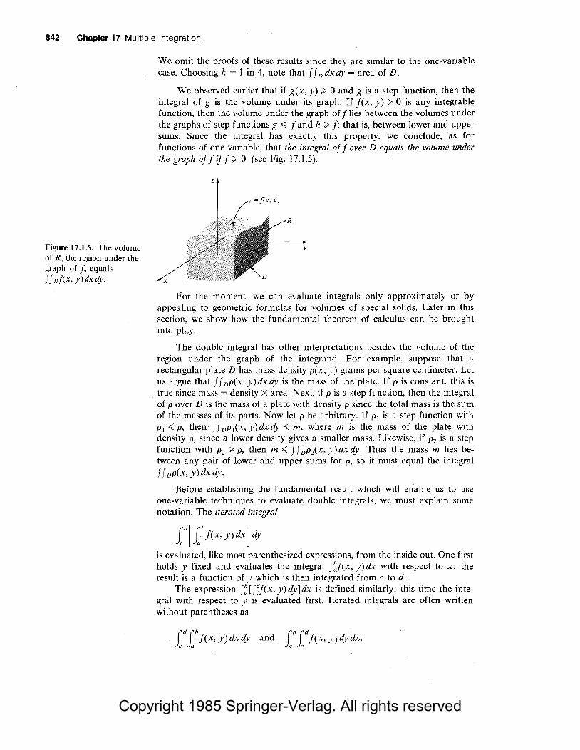
Copyright 1985 Springer-Verlag. All rights reserved
842 Chapter 17 Multiple Integration
Figure 17.1.5. The volume of R, the region under the graph of f, equals ff nf(x, y) dx dy.
We omit the proofs of these results since they are similar to the one-variable case. Choosing k = 1 in 4, note that ff D dx dy = area of D.
We observed earlier that if g(x, y) > 0 and g is a step function, then the integral of g is the volume under its graph. If f(x, y) > 0 is any integrable function, then the volume under the graph off lies between the volumes under the graphs of step functions g < f and h > f; that is, between lower and upper sums. Since the integral has exactly this property, we conclude, as for functions of one variable, that the integral off over D equals the volume under the graph off if f > 0 (see Fig. 17.1.5).
z
y
x
For the moment, we can evaluate integrals only approximately or by appealing to geometric formulas for volumes of special solids. Later in this section, we show how the fundamental theorem of calculus can be brought into play.
The double integral has other interpretations besides the volume of the region under the graph of the integrand. For example, suppose that a rectangular plate D has mass density p(x, y) grams per square centimeter. Let us argue that ff nP(X, y) dx dy is the mass of the plate. If p is constant, this is true since mass= density X area. Next, if pis a step function, then the integral of p over D is the mass of a plate with density p since the total mass is the sum of the masses of its parts. Now let p be arbitrary. If p 1 is a step function with p1 < p, then ff nP 1(x,y)dxdy < m, where mis the mass of the plate with density p, since a lower density gives a smaller mass. Likewise, if p2 is a step function with p2 > p, then m < ff ;pix, y)dx dy. Thus the mass m lies between any pair of lower and upper sums for p, so it must equal the integral ff nP(X, y)dx dy.
Before establishing the fundamental result which will enable us to use one-variable techniques to evaluate double integrals, we must explain some notation. The iterated integral
Ld[ Lb f(x, y)dx] dy
is evaluated, like most parenthesized expressions, from the inside out. One first holds y fixed and evaluates the integral f~(x, y)dx with respect to x; the result is a function of y which is then integrated from c to d.
The expression f~[f~f(x, y)dy]dx is defined similarly; this time the integral with respect to y is evaluated first. Iterated integrals are often written without parentheses as

Copyright 1985 Springer-Verlag. All rights reserved
Example 3
Solution
Figure 17.1.6. The area of the cross-section is the area under the graph of z = f(x, y) fromy = c to y = d (where x is fixed).
17.1 The Double Integral and Iterated Integral 843
2 ' Evaluate fo .r x2ydydx.
2 3 2( 3 ) r2( x2y2
/3
) ( J: x2ydydx= i J: x2ydy dx= Jo - 2- dx Jo I 0 I 0 y~ I
= fo2x2( t - ~) dx= 4fo2x2dx =4 ~31: = 332 .
Notice that the second step in this calculation is essentially the inverse of a partial differentiation. £
We claim, and shall prove below, that the double integral equals the iterated integral. That is, for D = [a,b] X [c,d],
J fo!(x, y)dxdy= id[ lb f(x, y)dx J dy= Lb[ id f(x, y)dy J dx.
To see why this might be so, let us suppose that j(x, y) ;;;;. 0, so that the integral ff Df(x, y)dx dy represents the volume of the region R under the graph of f. If we take this volume and slice it by a plane parallel to the yz plane at a distance x from the origin, we get a two-dimensional region whose area is given by A(x) = J~j(x, y)dy (see Fig. 17.1.6).
z z Graph of z = f(x,y)
z =f(x,y)
x A(x) =Jed f(x,y) dy
By Cavalieri's principle (Section 9.1 ), the total volume is the integral of the area function A (x). Thus,
J Lf(x, y)dxdy= volume of R = LbA (x)dx= Lb[ id f(x, y)dy] dx.
In the same way, if we use planes parallel to the xz plane, we get
J Lf(x, y)dxdy= id[ Lb f(x, y)dx] dy,
which is what we claimed. We see that Cavalieri's principle gives a geometric "proof" of the reduction to iterated integrals; in fact, it is more appropriate to take our proof below as a justification for Cavalieri's principle.
Theorem: Reduction to Iterated Integrals Assume that f(x,y) is integrable on the rectangle D = [a,b] x [c,d]. Then any iterated integral which exists is equal to the double integral; that is,

Copyright 1985 Springer-Verlag. All rights reserved
844 Chapter 17 Multiple Integration
Proof of the Reduction to
Iterated Integrals
To prove this theorem, we first show it is true for step functions. Let g be a step function, with g(x, y) = kiJ on (t;_ 1, t;) X (s1_ 1, s), so that
n,m J J, g(x,y)dxdy= 2: kiJ/:::,.t;/:::,.s1 . D i=l,j=I
If the summands kiJ M; l:::,.s1 are laid out in a rectangular array, they may be added by first adding along rows and then adding up the subtotals, as follows:
kn! /:::,.tn /:::,.sl ~ ( i*l kil /:::,.t;) /:::,.sl
kn2 /:::,.tn /:::,.s2 ~ ( i*l k;2 /:::,.t;) /:::,.s2
knm /:::,.tn /:::,.sm ~ ( i*l kim /:::,.ti) /:::,.sm
)~I ( i*l kij /:::,.t;) /:::,.sj
The coefficient of l:::,.s1 in the sum over the jth row, 2:,7= 1ku /:::,.t0 is equal to f~g(x, y)dx for any y with si_ 1 < y < si, since, for y fixed, g(x, y) is a step function of x. Thus the integral f~g(x, y) dx is a step function of y, and its integral with respect toy is the sum:
Ld[lbg(x,y)dx]dy= J~IC*1 ku/:::,.t;)/:::,.si= J Lg(x,y)dxdy.
Similarly, by summing first over columns and then over rows, we obtain
The theorem is therefore true for step functions. Now letf be integrable on D = [a,b] X [c,d] and assume that the iterated
integral f~[f~j(x, y)dy]dx exists. Denoting this integral by S0 , we will show that every lower sum for f on D is less than or equal to S0 , while every upper sum is greater than or equal to S0 , so S0 must be the integral off over D.
To carry out our program, let g be any step function such that
g(x, y) <; f(x, y) (1)
for all (x, y) in D. Integrating equation (1) with respect to y and usmg property 5 of the one-variable integral (see Section 4.5), we obtain
(2)
for all x in [a, b]. Integrating (2) with respect to x and applying property 5 once more gives
(3)
Since g is a step function, it follows from the first part of this proof that the left-hand side of (3) is equal to the lower sum ff ng(x, y) dx dy; the right-hand side of (3) is just S0 , so we have shown that every lower sum is less than or equal to S0 . The proof that every upper sum is greater than or equal to S0 is similar, and so we are done. •

Copyright 1985 Springer-Verlag. All rights reserved
17.1 The Double Integral and Iterated Integral 845
Example 4 Let j(x, y) = e2x+ Y, Evaluate the integral off over D = [O, l] x [O, 3].
Solution J foJ(x,y)dxdy= fo3(fo
1e2x+ydx)dy
= (3(le2x+y11 )dy=l (3(e2+y_eY)dy Jo 2 x=O 2 Jo
1 r3 ( e2 - 1 )( e3
- 1) = 2 ( e
2 - 1) Jo eY dy= 2
~ 60.9693.
(You should check that integrating with respect to y first gives the same answer.) .A.
Example 5 Evaluate i 3 fo
2 xy dx dy and compare with Example 3.
Solution fi 3 fo2xydxdy= fi 3
(fo2xydx) dy= fi 3
( x? 1:=J dy
= (3
_§_ ydy = 1y213=1 (32 - 12) = 32 .
J1 3 3 I 3 3
The answer is the same as that in Example 3, as predicted by the theorem above. (It is also consistent with Examplj:: 2.) .A.
Example 6 Compute J fosin(x + y)dxdy, where D = [0,'1T] X [0,2'17].
Solution J fosin(x + y)dxdy= fo2'1T[ fo'1Tsin(x + y)dx] dy
= fo2
'1T[ -cos(x + y)l:=o] dy
= fo 2'1T[ cosy - cos(y + '1T) J dy
= [ siny- sin(y + '1T)Jl;: 0 = 0 . .A.
Example 7 Find the volume under the graph of f(x, y) = x 2 + y 2 between the planes x = 0, x = 3, y = -1, and y = 1.
Solution The volume is
J_\fo3(x
2 + y 2)dxdy= L\( ~3
+ y2xl~=J dy= j_\(9 + 3y2)dy
= (9y + y3)l~1 = 20 ....
Example 8 If D is a plate defined by 1 < x < 2, 0 < y < l, and the mass density is p(x, y) = yexy grams per square centimeter, find the mass of the plate.
Solution The total mass is

Copyright 1985 Springer-Verlag. All rights reserved
846 Chapter 17 Multiple Integration
I ( 2y )j' =Ia (e2y _ eY)dy= T -eY ro
e2 I = 2 - e + 2 ~ 1.4762 grams . .6.
Supplement for Section 17 .1: Solar Energy and Double Integrals
To illustrate the process of summation which is represented by the double integral, we may use an example connected with solar energy. The intensity of solar radiation is a "local" quantity, which may be measured at any point on the earth's surface. Since the s9lar intensity is really a rate of power input (see the Supplement to Section 9.5), we can measure it in units of watts per square meter.
If the solar intensity is uniform over a region, the total power received is equal to the intensity times the area of the region. In practice, the intensity is a function of position (in particular, it is a function of latitude); so we cannot just multiply a value by the area of the region. Instead, we must integrate the intensity over the region. Thus, the method of this section would allow us to find (at least in principle) the total power received by the state of Colorado, which is a rectangle in longitude-latitude coordinates. The problem for Utah is also tractable, since that state is composed of two rectangles, but what happens if we are interested in Michigan or Florida? For this problem, we need to integrate over regions which are not rectangles: the method for doing this is presented in the next section.
Exercises for Section 17 .1 In Exercises I and 2, the function g takes values on the rectangles as indicated in Fig. 17.1.7. Calculate the integral of g.
I. For the rectangle in Fig. 17.l.7(a).
2. For the rectangle in Fig. 17.l.7(b).
y y
4 3
0 3 4
-2 2 I 3
2 -I -I -2 I 2
I I --2 I
-I -2 2 I 4 x 2 4 6 x
(a) (b)
Figure 17.1.7. Find the integral of g.
3. (a) Let D be the rectangle determined by the inequalities - I .;; x .;; I and 2 .;; y .;; 4 and let f(x, y) = x(l + y). Find a step function g satisfying g(x, y) < f(x, y) to show that ffnf(x,y)dxdy > -9. (b) Sketch the graph of f(x, y) over D. Use symmetry to argue that the value of the integral in part (a) must in fact be zero.
4. Let D be the rectangle I .;; x .;; 4, 0 .;; y .;; 2. Suppose that D is a plate with mass density p(x, y) = 2xy2 + cos'ITy + 1 (grams per square centimeter). Find step functions to show that the mass m (in grams) of the plate satisfies the inequalities 30 .;; m .;; 62.
Evaluate the iterated integrals in Exercises 5-10.
5. fo 3 fo 2x3ydxdy 6. fo 2fi 4
x 3ydydx
7. (2J 1
(yx)2 dy dx 8. J 1 (
2(yx)2 dx dy
Jo -1 -1Jo
9. J 1 (
1yex dy dx IO. J 1
(3y 5exy' dx dy
-1Jo -1Jo Evaluate J J nf(x, y) dx dy for the indicated functions and rectangles in Exercises 11-16.
11. j(x, y) = (x + 2y)2; D = [ -1, 2] X [O, 2]. 12. j(x, y) = y 3cos2x; D = [ - 'IT /2, 'IT] X [!, 2]. 13. f(x,y) = x 2 + 2xy - y{X; D = [O, I] X [-2,2]. 14. j(x, y) = xy3ex'r'; D = [!, 3] X [!, 2]. 15. f(x, y) = xy + x/(y + l); D = [1,4] X [1,2]. 16. f(x, y) = y5eY' cosx sin x; D = [O, 1] x [ -1, OJ.
17. Evaluate JiJ~ 1 x(l + y)dxdy and compare with Exercise 3.
18. Evaluate J~Ji(2xy2 + cos'ITy + l)dxdy and compare with Exercise 4.

Copyright 1985 Springer-Verlag. All rights reserved
17.1 The Double Integral and Iterated Integral 847
Sketch and find the volume under the graph of f between the planes x = a, x = b, y = c, and y = d in Exercises 19 and 20.
19. j(x,y)=x 3 + y 2 +2; a= -1, b= I, c= I, d= 3.
20. j(x, y) = 2x + 3y2 + 2; a= 0, b = 3, c = - 2, d =I.
21. The density at each point of a 1 centimeter square (i.e., each side has length 1 centimeter) microchip is 4 + r2 grams per square centimeter, where r is the distance in centimeters from the point to the center of the chip. What is the mass of the chip?
22. Do as in Exercise 21, but now let r be the distance to the lower left-hand corner of the plate.
*23. Prove that the sum of two step functions defined on the same rectangle is again a step function.
*24. Prove that if j(x, y) .;; g(x, y) for all (x, y) in the rectangle [a,b] x [c,d], then
lb ld f(x, y) dydx <ld lh g(x,y)dxdy.
*25. The state of Colorado occupies the region between 33° and 41° latitude and 102° and 108° longitude. A degree of latitude is about 110 kilometers and a degree of longitude is about 83 kilometers. The intensity of solar radiation at time I on day T at latitude l is (in suitable units; see the Supplement to Section 9.5)
I = cos l 1 - sin2a cos2( ~~~) cos(
22~1
)
. l . ( 2wT) + Sill Sill a COS 365
.
(a) What is the integrated solar energy over Colorado at time I on day T?
(b) Suppose that the result of part (a) is integrated with respect to I from 11 to 12. What does the integral represent?
17 .2 The Double Integral Over General Regions
Figure 17.2.1. Givenf and D, we constructf* by settingf*(x, y) equal to zero outside D.
Double integrals over general regions become iterated integrals with variable endpoints.
Many applications involve double integrals J J nf(x, y) dx dy over regions D which are not rectangles. For instance, the volume of a hemisphere, the mass of an elliptical plate, or the total solar power received by the state of Texas can be expressed as such integrals. We shall find that such integrals can be evaluated by iterated integration in a form slightly more complicated than that used for rectangles.
To begin, we must define what we mean by ff nf(x, y)dxdy when Dis not a rectangle. We shall assume that D is contained in some rectangle D*. Let f* be the function on D* defined by
if f*(x, y) = { ~(x, y)
if
(See Fig. 17.2.1.)
z = f(x,y)
_,,,,..-) !' ...... ~ ..,,,
f"---- I I I I I I I I I
t:D
(x,y) ED,
(x,y) fl. D.
• y

Copyright 1985 Springer-Verlag. All rights reserved
848 Chapter 17 Multiple Integration
Figure 17.2.2. The choice of D* does not matter.
y
y
y = ¢1(x)
x
x
Figure 17.2.3. A region Dis of type I if it is the region between the graphs of two functions,y = cj> 1(x) and y = c/>2(x).
If D** is another rectangle containing D, and f** is the corresponding function defined as above, then JJD*J*(x,y)dxdy =ff D··f**(x,y)dxdy, since J* and J** are zero in the regions where D* and D** differ (see Fig. 17.2.2 and use the properties of the integral given in Section 17.l ).
f' and /* * are zero here
D'
D"
We note that if j(x, y) > 0 on D, then both integrals above are equal to the volume of the region under the graph off on D, i.e., the set of (x, y, z) such that (x, y) E D and 0 < z < f(x, y).
With these preliminaries, we can state the following definition.
The Double Integral Over a Region D Extendf to a rectangle D* containing D by lettingf* equalf on D and zero outside D. IfJ* is integrable on D*, then we say thatfis integrable on D, and we define Jf Df(x,y) dxdy to be JJD*J*(x,y)dxdy. (By our preceding remarks, the choice of D* does not affect the answer).
This definition serves the purpose of giving meaning to the double integral, but it is not very useful for computation. For this purpose, we need to choose D in a more specific way. We shall define two simple types of regions, which we will call elementary regions. Complicated regions can often be broken into elementary ones.
Suppose that we are given two continuous real-valued functions <f> 1 and <f>2 on [a,b] which satisfy <f> 1(t) < <f>i(t) for all tin [a,b]. Let D be the set of all points (x, y) such that
xisin[a,b] and </> 1(x)<y<</>2(x).
This region D is said to be of type 1. (See Fig. 17.2.3.) The curves and straight line segments that enclose the region constitute the boundary of D.
We say that a region D is of type 2 if there are continuous functions if;1
and if;2 on [ c, d] such that D is the set of points ( x, y) satisfying
y is in [ c, d] and if; 1(y) < x < if;i(y),
where if;1(t) < if;i(t) fort in [c,d]. (See Fig. 17.2.4.) Again the boundary of the region consists of the curves and line segments enclosing the region.

Copyright 1985 Springer-Verlag. All rights reserved
Figure 17.2.4. A region Dis of type 2 if it is the region between the graphs of x = 1h(y) and x = 1/;i(y).
17.2 The Double Integral Over General Regions 849
y y
x x
The following example shows that a given region may be of types 1 and 2 at the same time.
Example 1 Show that the region D defined by x 2 + y 2 < 1 (the unit disk) is a region of types 1 and 2.
Solution Descriptions of the disk, showing that it is of both types, are given in Fig. 17.2.5 .....
Figure 17.2.5. The unit disk as a type I region and a type 2 region.
y=rf>z(X)
y =rf>1(X)
Figure 17.2.6. The integral off* over D* equals that of f over D.
y y
x = >J; 1(y)
=-v1J7
- I x x
y = rf>1(X) - I
=-~
(a) Type I region (b) Type 2 region
We will use, without proof, 1 the following fact: If J is continuous on an elementary region D, then J is integrable on D. This fact, combined with the reduction to iterated integrals for rectangles, enables us to evaluate integrals over elementary regions by iterated integration. Indeed, if D* = [a,b] X [c,d] is a rectangle containing D, then
J fnJ(x, y)dxdy = J LJ*(x, y)dxdy =Lb Ld f*(x, y)dydx
= Ld ih 1*c x, y) dx dy,
(1)
(2)
where f* equals f in D and is zero outside D. Assume that D is a region of type 1 determined by functions </> 1 and </>2 on [a, b ]. Consider the iterated integral
ib Ld f*(x, y)dydx
and, in particular, the inner integral J~J*(x, y)dy for some fixed x (Fig. 17.2.6). By definition,J*(x, y) = 0 if y < <f> 1(x) or y > <f> 2(x), so
(d J*( x, Y) dy = l'MxJ f*( x, y) dy = l<1>2(x) f( x, y) dy. (3) Jc ¢1(x) ¢1(x)
1 For a proof, see an advanced calculus text, such as J. Marsden, Elementary Classical Analysis, Freeman (1974), Chapter 8.

Copyright 1985 Springer-Verlag. All rights reserved
850 Chapter 17 Multiple Integration
y
\ I
' 4 '-......
Substituting (3) into (1) gives
f J, f( x, y) dx dy =lb[ (c/>2(x) f( x, y) dy] dx.
D a Jcp,(x)
A similar construction works for type 2 regions.
Double Integrals If D is a r,egion of type 1 (Fig. 17.2.3),
f J, f(x, y) dx dy= lb[ (c/>2(x) f(x, y) dy] dx. D a Jcp,(x)
If D is of type .2 (Fig. 17.2.4),
ff, f(x,y)dxdy= rd[ (>h(y)f(x,y)dx]dy. D Jc J.p,(y)
If D is of both types, either ( 4) or ( 5) is applicable.
(4)
(5)
If j(x, y) > 0 on D, we may understand the procedure of iterated integration as our old technique of finding volumes by slicing (Section 9.1). Suppose, for instance, that Dis of type 1, determined by <j> 1(x) and <j>z(x) on [a,b]. If we fix x and slice the volume under the graph of j(x, y) on D by the plane which passes through the point (x, 0, 0) and which is parallel to the yz plane, we obtain the region in the yz plane defined by the inequalities <j> 1(x) < y < <j>2(x) and 0 < z < j(x, y). The area A (x) of this region is just J!~/;jJ(x, y)dy. Now the double integral ff Df(x, y)dx dy, which is the volume of the entire solid, equals
lb A (x) dx =lb[ (c/>2(x) f( x, y) dy] dx,
a a Jcp,(x)
the iterated integral. Thus we get (4). If D is of type 2, then slicing by planes parallel to the xz plane produces
the corresponding result (5). The reader should draw figures similar to Fig. 17.1.6 to accompany this discussion.
Example 2 Find f L (x + y)dx dy, where Dis the shaded region in Fig. 17.2.7.
Solution D is a region of type 1, with [a,b] = [0,-!-J; cp 1(x) = 0, and cpz(x) = x 2• By
formula (4) in the preceding box,
y = x2
""!
I 2
I
D
x
J J,,(x + y)dxdr r'f'<x + y)dydx~ r'[ ( xy + i' (J dx
= (1/2(x3 + x4 )dx=( x4 + xs )11;2 Jo 2 4 10 .·.
•. 0
1 1 3 Figure 17.2.7. Find ff D(x + y)dx dy.
= 64 + 320 = 160 .
Dis also a region of type 2, with 1h(y) = fY and 1/iz(y) =~-We leave it to you to verify that the double integral calculated by formula (5) is also 1 ~0 • .A.

Copyright 1985 Springer-Verlag. All rights reserved
Example 3
17.2 The Double Integral Over General Regions 851
Evaluate (' fX\ydydx. Sketch the region for the corresponding double Jo Jx 3
integral.
y Solution Here y ranges from x 3 to x 2, while x goes from 0 to 1. Hence the region is as
shown in Fig. 17 .2.8. The integral is
Y =x3
x =I
Figure 17.2.8. The region of integration for J6J~ixy dy dx.
x
Example 4
The next example shows that it sometimes saves labor to reverse the order of integration.
Write fo 1fov't-x 2 Vl - y 2 dydx as an integral over a region. Sketch the region
and show that it is of types 1 and 2. Reverse the order of integration and evaluate.
y
Solution The region D is shown in Fig. 17.2.9. D is a type 1 region with <f> 1(x) = 0,
cf>i(x) = ./1 - x 2 and a type 2 region with i/;i(y) = 0, if;i(y) = Vl - y 2 . Thus
x
Figure 17.2.9. The region of integration for
f6JoVI-x' ,/I - y 2 dydx.
Example 5
fo'fo'/1-x2 Vl - Y2 dydx= fo'fov1-y2 Vl - Y2 dxdy
= r'[~ xlJI-y'] dy= r\1 - y 2)dy Jo x~O Jo
= ( y - ~3
) 1: = t . Evaluating the integral m the original order requires considerably more computation! .._
Calculate the integral of j(x, y) = (x + y)2 over the reg10n shown m Fig. 17.2.10.
Solution In this example, there is a preferred order of integration for geometric reasons. The order Jfj(x, y)dx dy, i.e., x first, requires us to break up the region into
y (2, 2) two parts by drawing the line y = 1; one then applies formula (5) to each part and adds the results. If we use the other order, we can cover the whole region at once:
(0,0) x
Figure 17.2.10. The region of integration for Example 5.
J fnJ(x,y)dxdy= fo2L~x+lf(x,y)dydx.
(The lines bounding D on the bottom and top are y = x and y = t x + I.) The integral is thus
i2i~x+I 2 l2[ 1 l*x+IJ - (x+y)dydx= 3 (x+y) 3- dx
0 x 0 y~x

Copyright 1985 Springer-Verlag. All rights reserved
852 Chapter 17 Multiple Integration
y
General regions can often be broken into elementary regions, and double integrals over these regions can be computed one piece at a time.
Example 6 Find J L x 2 dx dy, where R is the shaded region in Fig. 17.2.11.
Solution
x
Each of the regions R 1, R 2 , R 3 , R4 is of types 1 and 2, so we may integrate over each one separately and sum the results. Using formula (4), we get
I I I II J L,x2dx,dy= fa L x 2
dydx= fo (xy) y=xdx
(I (x3 x4)\1
=Jo(x2-x3)dx= 3-4 o
Similarly, we find
Figure 17.2.11. Integrate x 2
over the pinwheel.
J L2
x 2 dxdy= J_0
1fo-xx 2dydx= j,-.
By symmetry,
J L3
x2dxdy= A and J L.x
2dxdy= j,-,
so
Jl 2 1 1 1 1 2 Rx dxdy= TI+ 4 +TI+ 4 = 3 ·
You may check that formula (5) gives the same answers . .A.
Exercises for Section 17 .2 In Exercises 1-4, sketch each region and tell whether it is of type 1, type 2, both, or neither.
y
1. (x, y) such that 0 < y < 3x, 0 < x < 1. 2. (x,y) such thaty 2 < x < y, 0,;;:; y < 1. 3. (x, y) such that x 4 + y 4
,;;:; 1.
4. (x, y) such that ~ ,;;:; x 4 + y 4,;;:; 1.
5. Find ff D(x + y)2dxdy, where Dis the shaded region in Fig. 17.2.12.
y =x
x = 1 x
Figure 17.2.12. The region of integration for Exercises 5 and 6.
6. Find JJD(l - sin?Tx)ydxdy, where Dis the region in Figure 17.2.12.
7. Find J J D(x - y)2dx dy, where D is the region in Figure 17.2.13.
8. Find Jf Dy(l - cos(?Tx/4))dxdy, where Dis the region in Fig. 17.2.13.
y
y=vx
Figure 17.2.13. The region of integration for Exercises 7 and 8.
x

Copyright 1985 Springer-Verlag. All rights reserved
Evaluate the integrals in Exercises 9-16. Sketch and identify the type of the region (corresponding to the way the integral is written).
9. ("ihinxx(l + y)dydx. Jo smx
10. (' rxcos 2"\x2 + xy + l)dydx. Jo Jx-1
11. J' J<Z-y)2(y{X + y 3 - 2y)dx dy.
- I y2/3
12_ (2J3(,/4-x2
)/2 (-5- +y3)dydx. Jo -3(,/4-x2 )/2 ,/2 + x
13. fo'fox2(x2 + xy - y2)dydx.
14. (4Jy' 3 dx dy.
Jz y 2 -1
15. (' (\x + y)2dydx. Jo Jx 2
16. fo'fo 3Yex+ydxdy.
In Exercises 17-20, sketch the region of integration, interchange the order, and evaluate.
17. fo'L'xydydx
18. fo"/2 focos 9 COS() dr d()
19. (' (' (x + y 2)dxdy Jo J1-y
20. Ji4Jirx(x2+ y 2)dydx
17.2 The Double Integral Over General Regions 853
In Exercises 21-24, integrate the given function f over the given region D.
21. j(x, y) = x - y; D is the triangle with vertices (0, 0), (l, 0), and (2, 1).
22. j(x, y) = xy + cosx; D the triangle defined by 0 < x <'TT /2, 0 < y < x.
23. j(x, y) = (x 2 + 2xy2 + 2); D the region bounded by the graph of y = - x 2 + x, the x axis, and the lines x = 0 and x = 2.
24. j(x, y) = sin x cosy; D the pinwheel in Fig. 17.2.ll.
25. Show that evaluating ff D dx dy, where D is a region of type l, simply reproduces the formula from Section 4.6 for the area between curves.
26. Let D be the region defined by x 2 + y 2 < I. (a) Estimate ff D dx dy (the area of D) within
0.1 by taking a rectangular grid in the plane and counting the number of rectangles: (i) contained entirely in D (lower sum); (ii) intersecting D (upper sum).
(b) Compute ff D dx dy exactly by using an iterated integral.
27. Which states in the United States are regions of type I? Type 2? (Take x = longitude, y = latitude.)
*28. Prove: fox[ f F(u) du] dt = fo\x - u)F(u)du.
17 .3 Applications of
Figure 17.3.1. The region under the graph off on D may be thought of as being composed of infinitesimal rectangular prisms.
the Double Integral Volumes, centers of mass, and surface areas can be calculated using double integrals.
We have observed in Section 17.1 that if f(x, y) > 0 on D, then the double integral J J Df( x, y) dx dy represents the volume of the three-dimensional region R defined by (x, y) in D, 0 < z < f(x, y). An "infinitesimal argument" for this result goes as follows. Consider R to be made of "infinitesimal rectangular prisms" with base dx and dy and height f(x, y) (see Fig. 17.3.1). The total
y
x

Copyright 1985 Springer-Verlag. All rights reserved
854 Chapter 17 Multiple Integration
volume is obtained by integrating (that is, "summing") the volumes of these cylinders. Notice, in particular, that if j(x, y) is identically equal to 1, the volume of the region under the graph is just the area of D, so the area of D is equal to J Jn dx dy.
Example 1 Compute the volume of the solid in space bounded by the four planes x = 0, y = 0, z = 0, and 3x + 4y = 10, and the graph z = x 2 + y 2.
Solution The region is sketched in Fig. 17.3.2. Thus the volume is
Figure 17.3.2. The volume of the region in space above D and below z = x 2 + y 2
, is Jf n(x2 + y 2)dxdy.
J L ( x2 + y2) dx dy = fo5/2[ fo(I0-4y)/\ x2 + y2) dx] dy
= + dy i 5/2[ (10 - 4y)3
y2(10 - 4y) l
0 34 3
4 5/2 = - (10 - 4y) + 10y3 - y4 I
34 • 4. 4 9 3 0
=_ML+ 10. 53 _ L = 15625~ 12 _056 . .A. 34.24 32.23 3·24 1296
y
(The volume in Example 1 can also be written as 56 / (34
• 24). Can any reader
explain this simple factorization?)
By reasoning similar to that for one-variable calculus (see Section 9.3), we are led to the following definition of the average value of a function on a plane region.
Average Value If f is an integrable function on D, the ratio of the integral to the area of D,
J Lf(x,y)dxdy
J L dxdy
is called the average value off on D.
Example 2 Find the average value of j(x, y) = x sin2(xy) on D = [O, 'lT] X [O, 'lTj.
Solution First we compute
J Lf(x,y)dxdy= fo''fo,,.xsin2(xy)dxdy

Copyright 1985 Springer-Verlag. All rights reserved
17.3 Applications of the Double Integral 855
i71(i 71 1 - cos(2xy) ) i 71
( y sin2(xy)) 1
71
= xdy dx= - - x dx o o 2 o 2 4x
y=O
7T3 [ cos(27r2) - 1 J
=-+------4 87T
Thus the average value off is
7T3
/ 4 + [ cos(27r2) - 1 J /87r 7T cos(27T2
) - 1 --------- = -
4 +
3 ~o.7839. _...
7T2 87T
Double integration also allows us to find the center of mass of a plate with variable density. Let D represent a plate with variable density p(x, y). We can imagine breaking D into infinitesimal elements with mass p(x, y)dx dy; the total mass is thus ff nP(x, y)dx dy. Applying the consolidation principle (see Section 9.4) to the infinitesimal rectangles, one can derive the formulas in the following box.
Center of Mass
_ J fvxp(x,y)dxdy x=~~-----J Lp(x,y)dxdy
and _ J fvyp(x,y)dxdy y= J Lp(x, y)dxdy .
Example 3 Find the center of mass of the rectangle [O, l] x [O, 1] if the density is ex+y.
Solution First we compute the mass:
J fvex+ydxdy= fo 1fo 1ex+ydxdy= fo 1 (ex+yl~=o)dy
= fo\ el +y - eY)dy
= e 1+y - eYl~=o = e2 - e - (e - 1) = e2
- 2e +I.
The numerator in the formula for x is
so
I I I II ii xex+y dxdy= i (xex+y - ex+y) dy 0 0 0 x=O
x= e - 1
e2 - 2e + 1
= fo 1[ e1+y - e 1+Y - (OeY- eY) ]dy
= fo 1eYdy= eYl~=o = e - 1,
e - 1 = _l_ ~o.582. (e-1)2 e-1
The roles of x and y may be interchanged m all these calculations, so y = l/(e - l)~0.582 as well . ..&.

Copyright 1985 Springer-Verlag. All rights reserved
856 Chapter 17 Multiple Integration
Figure 17.3.3. The "image" on the surface z = j(x, y) of an infinitesimal rectangle in the plane is the infinitesimal parallelogram P1P2P4P3.
In Section 10.3 we used ordinary integration to determine the area of surfaces of revolution. Using the double integral, we can find the area of general curved surfaces. We confine ourselves here to an infinitesimal argument-the rigorous theory of surface area is quite subtle.2
To find the area of the graph z = j(x, y) of a function f over the plane region D, we divide D into "infinitesimal rectangles" which are of the form [x,x + dx] x [y, y + dy]. The image of this infinitesimal rectangle on the graph off is approximately an "infinitesimal parallelogram" with vertices at
P1 = (x, y, f(x, y)),
P2 = (x + dx, y, f(x + dx, y)) ~ (x + dx, y, f(x, y) + fx(x, y)dx),
P3 = (x,y + dy,f(x,y + dy))~(x,y + dy,f(x,y) + fy(x,y)dy),
P4 = (x + dx, y + dy, f(x + dx, y + dy))
~(x + dx,y + dy,f(x,y) + fx(x,y)dx + fy(x,y)dy).
(See Fig. 17.3.3.)
x
We compute the area dA of this parallelogram by taking the length of the cross product of the vectors from P1 to P2 and from P1 to P3 (see Section 13.5). The vectors in question are dxi + fx(x,y)dxk and dyj + fy(x,y)dyk; their cross product is
j dx 0
0 dy
k
fx(x, Y) dx = - fx(x, y) dx dy i - fy(x, y)dx dy j + dx dy k,
fy(x, y)dy
and the length of this vector is dA =-JI+ fx(x,y) 2 + fy(x,y) 2 dxdy. To get the area of the surface, we "sum" the areas of the infinitesimal parallelograms by integrating over D.
2 See T. Rado, Length and Area, American Mathematical Society Colloquium Publications, Volume 30 (1958).

Copyright 1985 Springer-Verlag. All rights reserved
17.3 Applications of the Double Integral 857
Surface Area of a Graph
Area= J LdA = J L J1 + fx(x, y)2 + fy( x, y)2 dx dy
Note the similarity of this expression with the formula for the arc length of a graph (Section 10.3). As with arc length, the square root makes the analytic evaluation of surface area integrals difficult or even impossible in all but a few accidentally simple cases.
Example 4 Find the surface area of the part of the sphere x 2 + y 2 + z2 = 1 lying above the ellipse x 2 + (y 2
/ a 2) < 1 ; (a is a constant satisfying 0 < a < 1 ).
Solution The region described by x 2 + (y 2 / a2) < 1 is type 1 with <f> 1(x) = - aJl - x 2
and <f>i(x) =a~; -1 < x < 1. The upper hemisphere may be described
by the equation z = j(x, y) = -j1 - x 2 - y 2
. The partial derivatives off are
az/ax=-x/-jl-x2-y2 and az/ay=-y/-jl-x2-y2 , so the area integrand is
Figure 17.3.4. The area of the hemisphere above the ellipse x 2 + y 2
/ a 2 <; I is 4 sin - 1a.
V 2 y2 1 + x + --'---
1 - x2 - y2 1 - x2 - y2 -j1 - x2 - y2
and the area is
A=f( dxdy
)D-jl-x2-y2 -JI [Ia~ dy ]dx
-I -a.jl-x2 -jJ _ X2 _ y2
= J_\(sin- 1 y 2
la./I-x2
)dx=2J_1
1sin- 1adx=4sin- 1a.
~ -a./l-x2
(See Fig. 17.3.4.) As a check on our answer, note that if a= I, we get 4 sin - 11 = 4 · 'TT /2 = 2'TT, the correct formula for the area of a hemisphere of radius I (the surface area of a full sphere of radius r is 47rr2
) . .&.

Copyright 1985 Springer-Verlag. All rights reserved
858 Chapter 17 Multiple Integration
Example 5 The equation in xyz space of the surface obtained by revolving the graph y = f(x) about the x axis is y 2 + z 2 = [f(x)]2. Express as a double integral the area of the part of this surface lying between the planes x = a and x = b. Carry out the integration over y. Do you recognize the resulting integral over x?
Solution Writing z as a function of x and y, we have z = g(x, y) = ± J f( x)2 - y 2 .
Figure 17.3.5. Finding the surface area when y = f(x) is rotated about the x axis.
The domain of this function consists of those (x, y) with - f(x) < y < f(x), so the surface in question lies over the type 1 region D defined by a < x < b, - f(x) < y < f(x). (See Fig. 17.3.5.) The partial derivatives of g are
,/ --y ~ -f(x) x
z
/ y
gx( x, y) = J'(x)f( x)/ V f( x)2 - y 2 , gy(x,y)= -y/Vf(x)2-y2,
so the surface area integrand is
and the area is A = 2 (bJJ(x) f( x) Ja -J(x)
f(x)2 - y2 + J'(x)2f(x)2 + y2
f(x)2 - y2
I+ J'(x)2
f(x)2 - y2 = f(x)
1 + J'(x)2 dydx.
f(x)2 - y2
(The factor of 2 occurs since half the surface lies below the xy plane.) We can carry out the integration over y:
A = 2 Jb f(x)Vl + J'(x)2 [Jj(x) l dy l dx a -j(x)Vf(x)2-y2 J
= 2 Jb f(x)Jl + J'(x)2 r sin- 1( f(~) )Jf(x) l dx
a l y~-j(x)
= 2 ib f(x)Rc---;)2 ( ~ + ~ )dx
= 27T ib f(x)JI + J'(x)2 dx.
This is the formula for the area of a surface of revolution (Section 10.3). J..

Copyright 1985 Springer-Verlag. All rights reserved
Exercises for Section 17 .3 In Exercises 1-4, find the volume under the graph of f(x, y) between the given planes x =a, x = b, y = c, andy = d,
l. f(x, y) = x sin y + 3; a= 0, b = 2, c ='TT, d= 3'!T;
2. f(x,y) = xy5 + 2x4 + 6; a= 0, b = 1, c = -1, d = 1.
3. f(x,y)=2x 4 +3y213; a= -1, b= 1, c=O,
d=2;
4. f(x, y) = xy~x2 + 3y2 ; a= 1, b = 2, c = 1,
d=2. 5. Compute the volume under the graph of f(x, y)
= 1 +sin( 'TTY /2) + x on the parallelogram in the xy plane with vertices (0, 0), (l, 2), (2, 0), (3, 2). Sketch.
6. Compute the volume under the graph of f(x, y) = 4x 2 + 3y2 + 27 on the disk of radius 2 centered at (0, 1). Sketch.
7. Compute the volume under the graph of f(x, y) = (cos y )e 1 - cos 2x + xy on the region bounded by the line y = 2x, the x axis, and the line x = 'TT/2.
8. Compute the volume between the graphs of the functions f(x, y) = 2x + 1 and g(x, y) = - x -3 y - 6 on the region bounded by the y axis and the curve x = 4 - y 2• Sketch.
9. Find the volume of the region bounded by the planes x = 0 and z = 0 and the surfaces x = -4y2 + 3, and z = x3y.
10. Find the volume of the region bounded by the planes x = 1, z = 0, y = x + 1, y = - x - l and the surface z = 2x 2 + y 4
•
In Exercises 11-14, find the average value of the given function on the given region.
11. f(x, y) = y sin xy; D = [O, 'TT] X [O, 'TT]. 12. f(x, y) = x 2 + y 2
; D =the ring between the circles x 2 +y2 =1- and x 2 + y 2 = l.
13. f(x, y) = ex+y; D =the triangle with vertices at (0, 0), (0, l ), and ( l, 0).
14. f(x, y) = l/(x + y); D = [e, e2] x [e, e2
].
Find the average value of x 2 + y 2 over each of the regions in Exercises 15-18.
15. The square [O, l] x [O, l]. 16. The square [a,a + 1] X [O, l], where a> 0. 17. The square [O, a] X [O, a], where a > 0. 18. The set of (x, y) such that x 2 + y 2 < a2.
19. Find the center of mass of the region between y = x 2 andy = x if the density is x + y.
20. Find the center of mass of the region between y = 0, y = x 2
, where 0 < x < 1 · 21. Find the center of mass of the disk determined
by (x - 1)2 + y 2 < l if the density is x 2•
22. Repeat Exercise 21 if the density is y 2•
17.3 Applications of the Double Integral 859
23. Find the area of the graph of the function f(x, y) = Hx 312 + y 312) which lies over the domain D = [O, l] x [O, 1].
24. Find the area cut out of the cylinder x 2 + z 2 = l by the cylinder x 2 + y 2 = l.
25. Calculate the area of the part of the cone z2
= x 2 + y 2 lying in the region of space defined by x ;;. 0, y ;;. 0, z < l.
26. Find the area of the portion of the cylinder x 2 + z2 = 4 which lies above the rectangle defined by - l < x < 1, 0 < y < 2.
27. Show that if a plate D has constant density, then the average values of x and y on D are the coordinates of the center of mass.
28. Find the center of mass of the region (composed of two pieces) bounded by y = x 3 and y = \fx if the density is (x - y)2
. Try to minimize your work by exploiting some symmetry in the problem.
29. (a) Prove that the area on a sphere of radius r cut out by a cone of angle cp is 27Tr2(1 - cos cp) (Fig. 17.3.6).
Figure 17.3.6. The area of the cap is 27Tr2(1 - cos cp ).
(b) A sphere of radius l sits with its center on the surface of a sphere of radius r > 1. Show that the area of surface on the second sphere cut out by the first sphere is 'TT. (Does something about this result surprise you?)
30. A uniform rectangular steel plate of sides a and b rotates about its center of gravity with constant angular velocity w. (a) Kinetic energy equals t(mass)(velocity)2
.
Argue that the kinetic energy of any element of mass p dx dy (p = constant) is given by p(w2 /2)(x2 + y 2) dx dy, provided the origin (0, 0) is placed at the center of gravity of the plate.
(b) Justify the formula for kinetic energy:
K.E.=J ( p w22 (x2 + y2)dxdy. Jplate
(c) Evaluate the integral, assuming that the plate is described by - a /2 < x < a /2, -b/2<y<b/2.

Copyright 1985 Springer-Verlag. All rights reserved
860 Chapter 17 Multiple Integration
31. A sculptured gold plate D is defined by 0 < x < 2'1T and 0 < y < 'TT (centimeters) and has mass density p(x, y) = y 2sin24x + 2 (grams per square centimeter). If gold sells for $7 per gram, how much is the gold in the plate worth?
*33. Express as a double integral the volume enclosed by the surface of revolution in Example 5. Carry out the integration over y and show that the resulting integral over x is a formula in Section 9.1.
*32. (a) Relate the integrand in the surface area formula to the angle between k and the normal to the surface z = j(x, y).
*34. Let n right circular cylinders of radius r intersect such that their axes lie in a plane, meeting at one point with equal angles. Find the volume of their intersection. (b) Express the ratio of the area of the graph off
over D to the area of D as the average value of some geometrically defined quantity.
17 .4 Triple Integrals
Figure 17.4.1. The box W= [a,b] X [c,d] X [p,q] consists of points (x, y,z)
Integrals over regions in three-dimensional space require the triple integral.
The basic ideas developed in Sections 17. l and 17.2 can be readily extended from double to triple integrals. As with double integrals, one of the most powerful evaluation methods is reduction to iterated integrals. A second important technique, which we discuss in Section 17.5, is the method of changing variables.
If the temperature inside an oven is not uniform, determining the average temperature involves "summing" the values of the temperature function at all points in the solid region enclosed by the oven walls. Such a sum is expressed mathematically as a triple integral.
We formalize the ideas just as we did for double integrals. Suppose that Wis a box (that is, rectangular parallelepiped) in space bounded by the planes x =a, x = b,y = c,y = d, and z = p, z = q, as in Fig. 17.4.1. We denote this
z
y
satisfying a < x < b, b
c < y < d, and p < z < q. x
box by [a,b] X [c,d] X [p,q]. Letf(x,y,z) be a function defined for (x,y,z) in W-that is, for
a < x < b, c < y < d, p < z < q.
In order to define the triple integral
J J fwf(x, y,z)dxdydz,

Copyright 1985 Springer-Verlag. All rights reserved
Figure 17.4.2. g has the value kijk on the small box wijk•
17.4 Triple Integrals 861
we first define the concept of a step function of three variables. A function g(x,y,z) defined on [a,b]X[c,d]X[p,q] is called a step
Junction if there are partitions
a=t0 <t1 <···<tn=b of [a,b],
c =So< s1 < · · · < sm = d of [ c, d],
p=r0 <r1 < ··· <r1 =q of [p,q]
such that g(x, y,z) has the constant value kiJk for (x, y,z) in the open box
W;1k =(ti_, ,ti) X (s1_ 1 ,s1) X (rk_ 1 ,rk)·
We cannot draw the graphs of functions of three variables; however, we can indicate the value kiJk associated with each box (see Fig. 17.4.2). The
y
g = kiik here
b
x
integral of g is defined as a sum of nm! terms: n,m,/
J J fwg(x, y,z) dx dy dz= i= l,J~. k= 1 kiJk(volume WiJk)
n,m,l
2: kiJk (D.t;) (D.s1) (D.rk)· i= l,j= I, k= I
If f is any function on W, its lower (respectively upper) sums are defined, as before, as the integrals of step functions g (respectively h) such that g(x, y,z) < f(x, y,z) (respectively h(x, y,z) > j(x, y,z)) for all points (x, y,z) in W.
The Triple Integral We say that f is integrable on W if there is a number S0 such that every S < S0 is a lower sum for f on W and every S > S0 is an upper sum. The number S0 is called the integral of J over W and is denoted by
J J fwf(x,y,z)dxdydz.
At this point you should look back at the basic properties of the double integrals listed in Section 17.1. Similar properties hold for triple integrals. Furthermore, there is a similar reduction to iterated integrals.

Copyright 1985 Springer-Verlag. All rights reserved
862 Chapter 17 Multiple Integration
Theorem: Reduction to Iterated Integrals Let f(x, y, z) be integrable on the box W =[a, b] x [c, d] x [p, q]. Then any iterated integral which exists is equal to the triple integral; that IS,
J J fwf(x,y,z)dxdydz= .lqidibf(x,y,z)dxdydz
= .lq lb id f(x, y,z)dydxdz
= ib.lqidf(x,y,z)dydzdx,
and so on. (There are six possible orders altogether.)
The proof of this result is just like the corresponding one in Section 17.1, so we omit it.
Example 1 (a) Let W be the box [O, l] x [ - 1, O] x [O, t ]. Evaluate
J J fw(x + 2y + 3z)2dxdydz.
(b) Verify that we get the same answer if the integration is done in the order y first, then z, and then x.
Solution (a) According to the reduction to iterated integrals, this integral may be evaluated as
Ll/3JO LI 2 (x + 2y + 3z) dxdydz 0 -1/2 0
L1; 3Jo [ (x + 2y + 3z/ 1
1 l = dydz 0 -1/2 3 x=O
= fo 113 J~112 t [ (1+2y+3z)3
- (2y + 3z)3
] dydz
= (1/3 214 [ (1+2y + 3z)4 - (2y + 3z)4]/o dz Jo y=-112
= fo 113
2~ [ (3z + 1)4
- 2(3z)4
+ (3z - 1)4] dz
= 24 ~ 15 [(3z+1}5-2(3z)5 +(3z-1)5 ]/~~o
= 24 ~ 15 C25
- 2) = l~ .
(b) J J fw(x+2y+3z)2dydzdx
i lil/JJO 2 = . (x+2y+3z) dydzdx 0 0 -1/2

Copyright 1985 Springer-Verlag. All rights reserved
17.4 Triple Integrals 863
1.11113[ (x+2y+3z)
3
1° l = 6
dzdx 0 0 y= -1/2
[
4 4 1/3 l = r1 l ( (x + 3z) - (x + 3z - 1) ) Jo 6 12 12 dx
z=O
l l [ l)S l S 2 SJ I l = 72 5 (x + + (x - ) - x x=O =TI· A
Example 2 Evaluate the integral of ex+y+z over the box [O, l] X [O, l] X [O, l].
(I I =Jo [ e2+z - 2el+z + e'J dz= [ e2+z - 2el+z + ez]o
= e3 - 3e2 + 3e - l = (e - 1)3
• A.
As in the two-variable case, we define the integral of a function f over a bounded region W by defining a new function f*, equal to f on W and zero outside W, and then setting
J J fwf(x, y,z)dxdydz= J J fwJ*(x, y,z)dxdydz,
where W* is any box containing the region W. As before, we restrict our attention to particularly simple regions. A
three-dimensional region W will be said to be of type I if there is an elementary region D in the xy plane and a pair of continuous functions, y 1(x, y) and yi(x, y) defined on D, such that W consists of those triples (x, y,z) for which (x, y) ED and y 1(x, y) < z < yi(x, y). The region D may itself be of type l or type 2, so there are two possible descriptions of a type I region:
a< x < b,
y 1(x,y) < z < ri(x,y) (if D is of type l) (l)
or
c.;;; y.;;; d,
(if D is of type 2). (2)
Figure 17.4.3 on the next page shows two regions of type I that are described by conditions (l) and (2), respectively.

Copyright 1985 Springer-Verlag. All rights reserved
864 Chapter 17 Multiple Integration
Figure 17.4.3. A region of type I lies between two graphs z = y 1(x, y) and z = Y2(x, y).
Figure 17.4.4. The three types of regions in space.
Figure 17.4.5. Regions in space can be of more than one type. This one is of all three types.
z z
z = 'Y 1(x,y)
d
y y
/ (a) (b)
A region W is of type II if it can be expressed in form (I) or (2) with the roles of x and z interchanged, and Wis of type III if it can be expressed in form (I) or (2) withy and z interchanged. See Fig. 17.4.4.
x
z
(a) Region of type I
Top and bottom are surfaces z = 'Y(X, y)
x
z
(b) Region of type II
Front and rear are surfaces x = p(z, y)
z
Left and right are surfacesy = o(x, z)
Notice that a given region may be of two or even three types at once. (See Fig. 17.4.5.) As with regions in the plane, we call a region of type I, II, or III in space an elementary region.
As a region of type I
x
z
A region
As a region of type II
y
As a region of type III

Copyright 1985 Springer-Verlag. All rights reserved
17.4 Triple Integrals 865
Example 3 Show that the unit ball x 2 + y 2 + z2 < 1 is a region of all three types.
Solution As a type I region, we can express it as
-1 < x < 1,
Figure 17.4.6. The unit ball described as a region of type I.
-~<y<~,
- V 1 - x2 - y2 < z < V 1 - x2 - y2 .
In doing this, we first write the top and bottom hemispheres as z =
Vl - x 2 - y 2 and z = -Vl - x 2 - y 2 , where x and y vary over the unit disk
(that is, - V 1 - x 2 < y < V 1 - x 2 and x varies between - 1 and 1 ). (See Fig. 17.4.6.) We write the region as a type II or III region in a similar manner by interchanging the roles of x, y, and z in the defining inequalities. A
y = ¢2 (x) = vT=X2
y
As with integrals in the plane, any function of three variables which is continuous over an elementary region is integrable on that region. An argument like that for double integrals shows that a triple integral over an elementary region can be rewritten as an iterated integral in which the limits of integration are functions. The formulas for such iterated integrals are given in the following display.
Triple Integrals Suppose that Wis of type I. Then either
ff ( f(x,y,z)dxdydz=lb (<l>z(x)iy2(x,y)f(x,y,z)dzdydx (3) Jw a J</> 1(x) y 1(x,y)
(see Fig. 17.4.3(a)) or
ff ( f(x,y,z)dxdydz= (d (•/'2(y)iy2(x,y)f(x,y,z)dzdxdy (4) Jw Jc J,/Ji(y) y 1(x,y)
(see Fig. 17.4.3(b)).
If Wis of type II, it can be expressed as the set of all (x, y,z) such that
a< z < b, <P 1(z) < y < cpl(z), p1(z, y) < x < pl(z, y).

Copyright 1985 Springer-Verlag. All rights reserved
866 Chapter 17 Multiple Integration
Then
ff ( f(x,y,z)dxdydz= (b (<i>i(z) (Pi(z,y)f(x,y,z)dxdydz. (5)
Jw Ja J</>1(z) Jp 1(z,y)
If Wis expressed as the set of all (x, y,z) such that
c < y < d, i/; 1(y) < z < i/;2(y), p1(z, y) < x < pl(z, y),
then
ff ( f(x,y,z)dxdydz= (dlt/Jz(y) (Pi(z,y)f(x,y,z)dxdzdy. (6)
Jw Jc t/; 1(y) Jp,(z,y)
There are similar formulas for type III regions (Exercise 22). Another way to write formula (3) is
ff ( f( x, y, z) dx dy dz= f J, [ (ri(x,y) f( x, y, z) dz] dy dx, Jw D )y1(x,y)
and for formula ( 4),
ff ( f(x, y,z)dxdydz=fJ, [ (r2(x,y) f(x, y,z)dz] dxdy. Jw D Jy,(x,y)
Notice that the triple integral ff f w dx dy dz is simply the volume of W.
Example 4 Verify the formula for the volume of a ball of radius 1: ff f w dx dy dz = 1 w, where Wis the set of (x, y,z) with x 2 + y 2 + z2 ,;;;; I.
Solution As explained in Example 3, the ball is a region of type I. By formula (3), the integral is
JI J-J1-x2 jJ1-x2-y2 dzdydx.
-I --./l-x 2 -Ji-x2 -y2
Holding y and x fixed and integrating with respect to z yields
J_\J_-V~[ zl~\/i~2;,~2Y2 J dydx
= 2JI [J-J1-x22 (1 - x2 - y2)1;2 dy] dx. -I-~
Since x is fixed in the integral over y, this integral can be expressed as fG_a(a 2 - y 2)112dy, where a= (I - x 2)112. This integral represents the area of a semicircular region of radius a, so that ·
f a ( 2 2)I/2d a2 a -y ~=-w. -a 2
(We could also have used a trigonometric substitution.) Thus
J-./l-x2 (l 2 2)I/2d _ 1 - x 2
-x -y ~----'TT,
--./J-x2 2
and so
2J1 J-J1-x2 (1 - x2 - y2//2 dydx= 2J1 'TT 1 - x2 dx -I --./1-x2 -I 2

Copyright 1985 Springer-Verlag. All rights reserved
17.4 Triple Integrals 867
Example 5 Let W be the region bounded by the planes x = 0, y = 0, and z = 2, and the surface z = x 2 + y2. Compute ff f wx dx dy dz and sketch the region.
Solution Method I. The region Wis sketched in Fig. 17.4.7. We may write this as a region of type I with y 1(x, y) = x 2 + y 2
, yi(x, y) = 2, <j> 1(x) = 0, <j>i(x) =
Figure 17.4.7. Wis the region below the plane z = 2, above the paraboloid z = x 2 + y 2
, and on the positive sides of the planes x = O,y = 0.
Figure 17.4.8. Was a type
b- x2, a= 0, and b =fl. By formula (3),
(i2 (,/2-x2 2 2 =Jo Jo x(2-x -y)dydx
[
2 2 3/2
= foJ2 x (2 - x2)J/2 - ( - ; ) l dx
2 5 /2 fi -2(2 _ x) I
15 0
2s12 s{f =2·-=-15 15 .
z
z=2='Y2 (x,y)
x
Method 2. W can be expressed as the set of (x, y, z) with the property that p1(z, y) = 0 < x < (z - y 2
)1
/2 = pi(z, y) and (z, y) in D, where Dis the subset
of theyz plane with 0 < z < 2 and 0 < y < z 112 (see Fig. 17.4.8). Therefore,
z
D
x = P1(z,y) = 0
y
II region. x

Copyright 1985 Springer-Verlag. All rights reserved
868 Chapter 17 Multiple Integration
ff ( x dx dy dz = f J, ( ( P2(z,y)x dx) dy dz Jw D JP1(z,y)
- xdx dy dz - -- dydz -L2[lz1/2(l(z-y2)1/2 ) ] -L2lzl/2( z _ y2) 0 0 0 0 0 2
= l r2(z3/2 - z3/2 ) dz = l (2 'l:_ z3/2 dz 2 Jo 3 2 Jo 3
= [ _1_ s;2]2 = _1_ 2s12 = s{i 15 z 0 15 15 '
which agrees with our other answer . .._
Example 6 Evaluate (I rx (I dz dy dx. Sketch the region w of integration and interJo Jo Jx2+y2
pret.
Solution (1
(X (1
dzdydx= (' (\1 - x 2 - y 2)dydx Jo Jo Jx2+ y2 Jo Jo
=ii( x - x3 - ~3) dx= 1- i- /2 = i. This is the volume of the region sketched in Fig. 17.4.9 . .._
Figure 17.4.9. The region W (type I) for Example 6. x
Exercises for Section 17 .4
z
I. Evaluate J J J w(2x + 3y + z) dx dy dz, where W = (1, 2] X [ -1, l] X (0, l], in at least two ways.
2. Evaluate the integral J J J wx 2 dx dy dz, where W = (0, l] X [ -1, l] X (0, l], in at least two ways.
3. Integrate the function sin(x + y + z) over the box [0,'IT] X [0,'IT] x [0,'IT].
4. Integrate zex+y over (0, l] X (0, l] X (0, l]. Determine whether each of the regions in Exercises 5-8 is of type I, II, or III.
5. The region between the cone z = ~x2 + y 2 and the paraboloid z = x 2 + y 2
•
6. The region cut out of the ball x 2 + y 2 + z 2 ,;;; 4 by the elliptic cylinder 2x2 + z 2 = l i.e. the region inside the cylinder and the ball.
w z=x2+y2
Y =x
y
7. The region inside the ellipsoid x 2 + 2y2 + z 2 = 1 and above the plane z = 0.
8. The region bounded by the planes x = 0, y = 0, z = 0, x + y = 4, and x = z - y - 1.
Find the volumes of the regions in Exercises 9-12. 9. The region bounded by z = x 2 + y 2 and z =
10- x 2 - 2y2.
10. The solid bounded by x 2 + 2y2 = 2, z = 0, and x + y + 2z = 2.
II. The solid bounded by x = y, z = O,y = 0, x =I, and x + y + z = 0.
12. The region common to the intersecting cylinders x 2 + y 2 < a2 and x 2 + z 2 < a2
.

Copyright 1985 Springer-Verlag. All rights reserved
17.5 Integrals in Polar, Cylindrical, and Spherical Coordinates 869
Evaluate the integrals in Exercises 13-20.
13. fo1Ji 2 lz3
cos[7r(x + y + z)]dxdydz.
14. fol fox foY(y + xz)dzdydx.
15. J J L(x2 + y 2 + z 2)dxdydz; R is the region
bounded by x + y + z =a (where a> 0), x = 0, y = 0, and z = 0.
16. J J J wz dx dy dz; W is the region bounded by
the planes x = 0, y = 0, z = 0, z = 1, and the cylinder x 2 + y 2 = 1, with x > 0, y > 0.
17. J J J wx 2coszdxdydz; Wis the region
bounded by z = 0, z = 7T, y = 0, y = 1, x = 0, and x + y = 1.
18. fo2foxfox+ydzdydx.
19. J J J w (1 - z 2) dx dy dz; W is the pyramid with
top vertex at (0, 0, 1) and base vertices at (0, 0), (1,0), (0, 1), and (1, 1).
20. J J J w(x2 + y 2)dxdydz; Wis the same pyra-
mid as in Exercise 19.
21. If j(x, y, z) = F(x, y) for some function F-that is, if j(x, y, z) does not depend on z-what is the triple integral off over a box W?
22. Write general formulas analogous to (3) and (4) for the triple integral over a region of type III.
23. Do Example 4 by writing W as a region of type III.
24. Write out the property for triple integrals corresponding to property 2 of double integrals (Section 17. l, p. 841).
25. Show that the formula using triple integrals for the volume under the graph of a functionf(x, y), on an elementary region D in the plane, reduces to the double integral off over D.
26. (a) Sketch the region for the integral
f fox foy f(x, y, z) dz dy dx.
(b) Write the integral with the integration order dxdydz.
27. (a) Show that the triple integral of a product over a box is the product of three ordinary integrals; that is, if D = [a,b] x [c,d] x [p,q], then
J J foJ(x)g(y)h(z)dxdydz
= lbf(x)dx idg(y)dy Lqh(z)dz.
(b) Use the result of part (a) to do Example 2.
17 .5 Integrals in Polar,
Figure 17.5.1. The area of the infinitesimal shaded region is r dr d(}.
Cylindrical, and Spherical Coordinates Problems with symmetry are often simplified by using coordinates that respect that symmetry.
We deal first with polar coordinates. Recall that a double integral
J Jnf(x,y)dxdy
may be thought of as a "sum" of the values off over infinitesimal rectangles with area (dx) · (dy). As in Section 10.5, however, we can also describe a region using polar coordinates and can use infinitesimal regions appropriate to those coordinates. The area of such a region is rdrdO, as is evident from Fig. 17.5.1. If u = j(x, y), then u may be expressed in terms of r and (} by the formula u = j(rcosO,rsinO).
y
x
The preceding argument using infinitesimals suggests the formula in the following box (the rigorous proof is omitted).

Copyright 1985 Springer-Verlag. All rights reserved
870 Chapter 17 Multiple Integration
y
a
Double Integrals in Polar Coordinates
J Lf(x,y)dxdy= J Lf(rcosO,rsinO)rdrdO, (1)
where D' is the region corresponding to D in the variables rand 0.
Example 1 Evaluate J J e-<x2
+y2) dxdy, where Dais the disk x 2 + y 2 < a2•
Da
Solution The presence of r 2 = x 2 + y 2 in the integrand and the symmetry of the disk suggest a change to polar coordinates. The disk is described by 0 < r < a, 0 < (} < 27T, so by formula (I), we get
x
J L.e-<x2
+Y'ldxdy= fo 27Tfoae_'
2
rdrd0= fo 27T(- ~e-'2)1: d(}
I (27T , , = - l Jo (e-a - I)dO= 77(1 - e-a ).
There is no direct way to evaluate this integral in xy coordinates! .A.
There is a remarkable application of the result of Example I to single-variable calculus: we will evaluate the Gaussian integral f~
00e-x' dx, which is of basic
importance in probability theory and quantum mechanics. There is no known way to evaluate this integral directly using only single-variable calculus. If we bring in two-variable calculus, however, the solution is surprisingly simple. Letting a go to 00 in the formula ff D e -( x' + y') dx dy = 7T (I - e - a'), we find that the limit L = lima__,
00Jf v
0
e-<x'+ y')"dx dy exists and equals 7T. By analogy with the definition of improper integrals on the line, we may consider L as the (improper) integral of e-<x'+y') over the entire plane, since the disks Da grow to fill the whole plane as a~ oo. The rectangles Ra = [ - a, a] X [ - a, a] grow to fill the whole plane, too, so we must have
lim Jr e-(x'+y')dxdy= 7T a~co )Ra
as well3; but
3 The technical details of the proof that
lim J ( e-<x'+y'>dxdy= lim J ( e-<x'+y'>dxdy a--+oo Jna a--+oo )Ra
go as follows. We have already shown that
lim J ( e-<x'+y') dxdy a--+oo Jna
exists. Thus it suffices to show that
}~.n;,,(J _l0
e-<x'+y'ldxdy- J JD0
e.-<x'+y'>dxdy)
equals zero. The limit equals
Figure 17.5.2. Ca is the shaded region between Ra and Da.
lim J ( e-<x'+y') dxdy, a--+oo Jca
where c. is the region between Ra and Da (see Fig. 17.5.2). In the region Ca, )x2 + y 2 >a (the radius of D.), so e-<x'+y') .;;; e-•'. Thus

Copyright 1985 Springer-Verlag. All rights reserved
17.5 Integrals in Polar, Cylindrical, and Spherical Coordinates 871
Jr e-(x'+y') dxdy=fa fa e-(x'+y') dxdy=fa fa e-x'e-y' dxdy )Ra -a -a -a -a
where Ia= f"_ae-x' dx (see Exercise 27, Section 17.4). Thus,
e-x dx= im la= Joo 2 l' _
00 a---?oo
lim J r e - ( x' + y') dx dy a---?oo )Ra
The Gaussian Integral
J 00
e - x' dx = /:;; . -oo
Example 2 Find L: e- 2x' dx.
Solution We will use the change of variables y = /2 x to reduce the problem to the Gaussian integral just computed.
Joo -2x'd l' fa -2x'd l" Jfi.a -y' dy e x= im e x= im e --oo a-'>oo -a a-'>oo -ff.a /2
Example 3 Evaluate J .fnln(x2 + y 2)dxdy, where D is the region in the first quadrant
lying between the circles x 2 + y 2 = 1 and x 2 + y 2 = 4.
Solution In polar coordinates, D is described by the set of points (r, 0) such that 1 < r < 2, 0 < 0 < w /2. Hence
= e-a' area (ca)= e-a'(4a 2 - l'Ta 2) = (4 - 1'T)a 2e-a'.
Thus it is enough to show that lima__.00
a2e -a'= 0. But, by l'Hopital's rule (see Section 11.2),
lim a2e - a'= lim ( .E!__ ) = lim ( _lg_ ) = Jim ( _!_ ) = 0, a__,,.oo a--:,.oo ea2 a__,,.oo 2aea2 a-700 ea2
as required.

Copyright 1985 Springer-Verlag. All rights reserved
872 Chapter 17 Multiple Integration
Figure 17.5.3. The infinitesimal shaded region has volume r dr dB dz.
= f' 12 .C2(lnr) · rdrd()
= fon/2
( ~ (2lnr - l)CJ d() (integration by parts)
= fon/2( 4ln2 -1) dO= ~ ( 4ln2 -1 )·A We will now evaluate triple integrals in cylindrical and spherical coordinates. At this point you should review the basic features of these coordinates as discussed in Section 14.5.
Cylindrical coordinates consist of polar coordinates in the xy plane, together with the z coordinate. Therefore the infinitesimal "volume element" has volume rdrdOdz. See Fig. 17.5.3.
z
y
x
As in the case of polar coordinates, this leads us to a formula for multiple integrals, presented in the next box.
Triple Integrals in Cylindrical Coordinates
J J f wf( x, y, z) dx dy dz= J J f w/(r cos 0, r sin 0, z)r dr d() dz (2)
where W' is the region in r, (), z coordinates corresponding to W.
Example 4 Evaluate J J f w(z 2x 2 + zy2) dx dy dz, where Wis the cyljndrical region deter
mined by x 2 + y 2 < 1, -1 < z < 1.
Solution By Formula (2) we have
J J fw(z 2x2+zy2)dxdydz= J_\fo
2nfo\z2r2)rdrd0dz
= J_l i2nz2~11 d()dz l 0 r~O
Finally, we turn to spherical coordinates. The volume in space corresponding to infinitesimal changes dp, d(), and def> is shown in Fig. 17.5.4. The sides of this "box" have lengths dp, r dO( = p sin cf> dO), and p def> as shown. Therefore its volume is p2sin cf> dp d() def>. Hence we get the following:

Copyright 1985 Springer-Verlag. All rights reserved
Figure 17.5.4. The infinitesimal shaded region has volume p2sin <f> dp d(} def>.
Example 5
Solution
17.5 Integrals in Polar, Cylindrical, and Spherical Coordinates 873
Triple Integrals in Spherical Coordinates
J J fwf( x, y, z) dx dy dz
= J J fw.J(psincj>cosO,psincj>sinO,pcoscj>)p2sincj>dpdOdcj>, (3)
where W* is the region in p, 0, cj> space corresponding to W; i.e., the limits on p,O,cj> are chosen so that the region in xyz coordinates is W.
z
x
Find the volume of the ball x 2 + y 2 + z 2 .;;;; R 2 by using spherical coordinates.
The ball is described in spherical coordinates by 0 < 0 .;;;; 2'1T, 0 < cj> < 'IT, and 0 < p .;;;; R. Therefore, by formula (3),
J J f w dx dy dz= fo"' fo2"' fo R p2sin cj> dp dO dcj> = ~
3
fo"' fo2"' sin cj> dO dcj>
= 2'1Tf 3 fo"'sincj>dcj>= 2'1Tf 3 {-[ cos('IT)- cos(O)]}
4'1TR 3
=-3-
which is the familiar formula for the voh:1me of a ball. Compare the effort involved with Example 4, Section 17.4. A
Example 6 Evaluate J J fwexp[(x2 + y 2 + z2)312]dxdydz, where W is the unit ball;
i.e., the set of (x, y,z) satisfying x 2 + y 2 + z 2.;;;; 1.
Solution In spherical coordinates, W is described by
0 ~ p.;;;; 1,
Hence
0.;;;; cj>.;;;; 'IT, 0.;;;; 0.;;;; 2'1T.

Copyright 1985 Springer-Verlag. All rights reserved
874 Chapter 17 Multiple Integration
It is important to spend a few moments of reflection with each integral to decide whether cylindrical, spherical, or rectangular coordinates are most useful; usually the symmetry of the problem provides the needed clue.
Example 7 Find the volumes of the following regions:
(a) The solid bounded by the circular cylinder r = 2acosfJ, the cone z = r, and the plane z = 0.
(b) The solid bounded by the cone z = yx2 + y 2 and the paraboloid of revolution z = x 2 + y 2
•
(c) The region bounded by y = x 2, y = x + 2, 4z = x 2 + y 2, and z = x + 3.
Solution The formula for the volume of a region is J J J w dx dy dz.
y
Figure 17.5.5. The base of W for Example 7(a).
z
Figure 17 .5.6. A cross section of W for Example 7(b ).
x
(a) Since we can write r = 2a cos (J as r2 = 2ax or (x - a)2 + y 2 = a2, we see that the base of the solid is a circle in the xy plane centered at (a, 0) with radius a. (See Fig. 17.5.5.) The xz plane is a plane of symmetry, so theAotal volume is twice the volume over the shaded region. In cylindrical coordinates, the total volume is
x 2 fr/2 fo2a cos (J forr dz dr dfJ= 2 Io"' /2 fo2a cos (J(rzl~=o) dr d(J
= 2 ("'/2 r2acos(Jr2drdfJ= 2 ("'/2( r312acos0) d(J Jo Jo Jo 3 r=O
= 2 fo"'/2 8a3~os3(J dfJ= ( 1;a3 )fo"'l\1 - sin2fJ)cosfJdfJ.
Let u =sin(} to get (16a 3 /3)JM1 - u2)du = (16a3 /3)(u - u3 /3)lb = 32a3 /9. (b) In cylindrical coordinates, the solid is bounded by z = r and z = r2 (Fig. 17.5.6.) The solid is obtained by rotating the shaded area around the z axis. Thus, the volume is
l2.,,.l1ir L2.,,.L1 l2.,,.L1 2 3 rdzdrdfJ= (rzl~=,.i)drdfJ= (r - r )drdfJ
0 0 r2 0 0 0 0
= r2.,,.( r3 - r4 )II do= J_ r2.,,. do= '.!!.. • Jo 3 4 r=O 12 Jo 6
(c) This part does not require cylindrical or spherical coordinates; y = x 2 = x + 2 has the solutions x = - 1 and x = 2, so the volume is
J2 ix+2 rx+3 dzdydx=J2 ix+2[(x + 3)- x2 + y2] dydx
-1 x 2 J(x2+ y 2)/4 -1 x 2 4
= - + 4x - 3x - - + - + - dx f2 ( 16 2 4x
3 x4 x6
) -1 3 3 4. 12
== 16x + 2x2 _ x3 _ £ + £ + £ = 783 (
4 5 7 ) 12 3 : 3 20 84 _I 70 .
:
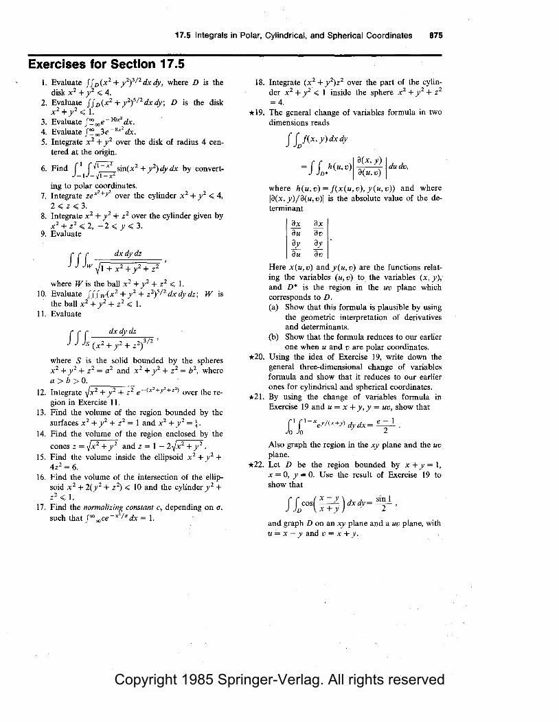
Copyright 1985 Springer-Verlag. All rights reserved
17.5 Integrals in Polar, Cylindrical, and Spherical Coordinates 875
Exercises for Section 17 .5 1. Evaluate J J D(x2 + y 2)312 dx dy, where D is the
disk x2 + y 2 .;;; 4. 2. Evaluate ff D(x2 + y 2)512 dx dy; D is the disk
x2 + y2.;;; 1. 3. Evaluate J'~ 00e- 10x2 dx. 4. Evaluate J~ 003e- 8x2
dx. 5. Integrate x2 + y 2 over the disk of radius 4 cen
tered at the origin.
6. Find J1 J~1 -x2 sin(x2 + y 2)dydx by convert
-I -..j!=? ing to polar coordinates.
7. Integrate zex2+Y
2 over the cylinder x2 + y 2 .;;; 4,
2.;;; z.;;; 3. 8. Integrate x2 + y2 + z2 over the cylinder given by
x 2 + z2 .;;; 2, - 2 .;;; y < 3.
9. Evaluate
J J l dxdydz w .Ji + x2 + y2 + z2 '
where W is the ball x2 + y 2 + z2 .;;; 1. 10. Evaluate ff J w(x2 + y 2 + z2)512 dx dy dz; W is
the ball x2 + y 2 + z2 .;;; 1. 11. Evaluate
JJL dxdydz 3/2 ' s ( x2 + y2 + z2)
where S is the solid bounded by the spheres x2 + y 2 + z 2 = a2 and x 2 + y 2 + z 2 = b2
, where a> b > 0.
12. Integrate -J'x72_+_y_,2,.-+-z"""2 e-<x2 +y'+z2) over the re-gion in Exercise 11.
13. Find the volume of the region bounded by the surfaces x2 + y 2 + z2 = 1 and x2 + y 2 = !.
14. Find the volume of the region enclosed by the
cones z = .Jx2 + y 2 and z = 1 - 2.Jx2 + y 2 •
15. Find the volume inside the ellipsoid x 2 + y 2 + 4z2 = 6.
16. Find the volume of the intersection of the ellipsoid x 2 + 2(y 2 + z2) .;;; 10 and the cylinder y 2 + z2.;;; 1.
17. Find the normalizing constant c, depending on a, such that J~ 00 ce-x
2/ 11 dx = 1.
18. Integrate (x2 + y 2)z2 over the part of the cylinder x 2 + y 2 .;;; 1 inside the sphere x 2 + y 2 + z 2
=4. * 19. The general change of variables formula in two
dimensions reads
J Lf(x,y)dxdy
= J L.h(u,v)I ~~:"~; ldudv,
where h(u, v) = f(x(u, v), y(u, v)) and where la(x, y)/a(u, v)I is the absolute value of the determinant
ax av ay av
Here x(u,v) and y(u,v) are the functions relating the variables ( u, v) to the variables ( x, y ), and D* is the region in the uv plane which corresponds to D. (a) Show that this formula is plausible by using
the geometric interpretation of derivatives and determinants.
(b) Show that the formula reduces to our earlier one when u and v are polar coordinates.
*20. Using the idea of Exercise 19, write down the general three-dimensional change of variables formula and show that it reduces to our earlier ones for cylindrical and spherical coordinates.
*21. By using the change of variables formula in Exercise 19 and u = x + y, y = uv, show that
(I (1-xey/(x+y) dydx= e - 1 . Jo Jo 2
Also graph the region in the xy plane and the uv plane.
* 22. Let D be the region bounded by x + y = 1, x = 0, y = 0. Use the result of Exercise 19 to show that
ff, cos( x - y) dxdy= sin 1 , D X + J 2
and graph D on an xy plane and a uv plane, with u = x - y and v = x + y.

Copyright 1985 Springer-Verlag. All rights reserved
876 Chapter 17 Multiple Integration
17 .6 Applications of Triple Integrals The calculation of mass and center of mass of a region in space involves triple int?grals.
Some of the applications in Section 17 .3 carry over directly from double to triple integrals. We can compute the volume, mass, and center of mass of a region with variable density p(x, y, z) by the formulas in the following box.
Volume, Mass, Center of Mass, and Average Value
Volume= J J fwdxdydz,
Mass= J J JJ>(x,y,z)dxdydz.
Center of mass= (.X, y,z), where
J J fwxp(x,y,z)dxdydz x = ---------
mass
_ J J fwyp(x,y,z)dxdydz y=
mass
J J fwzp(x,y,z)dxdydz z = ---------
mass The average value of a function f on a region W is defined by
J J fwf(x,y,z)dxdydz
J J fwdxdydz
(1)
(2)
(3)
Example 1 The cube [1,2] x [1,2] X [1,2] has mass density p(x,y,z) = (1 + x)ezy. Find the mass of the box.
Solution The mass of the box is
2 2[( 2) ]x=2 2 2 =Ii Ii x + ~ ey x=I dydz= J J !eydydz
= -ezdz= -ez J:2 15 [ 15 ]z=2 I 4 4 z=I
15 ( 2 = 4 e - e). A

Copyright 1985 Springer-Verlag. All rights reserved
17.6 Applications of Triple Integrals 877
Example 2 Find the center of mass of the hemispherical region W defined by the inequalities x 2 + y 2 + z2 ..;; 1, z ;;;.. 0. (Assume that the density is constant.)
Solution By symmetry, the center of mass must lie on the z axis, so x = y = 0. To find z, we must compute, by formula (2), I== J J J wz dx dy dz. The hemisphere is of types I, II, and III; we will consider it to be of type III. Then the integral I becomes
I= (1f,j1-z2 fJ1-y2-z2 zdxdydz. Jo -,/1-z2 -v1-y2-z2 Since z is a constant for the x and y integrations, we can bring it out to obtain
/= r1z(f,j1-z2 fv1-y2-z2 dxdy)dz. Jo -,j1-z2 -J1-y2-z2
Instead of calculating the inner two integrals explicitly, we observe that they are simply the double integral J JD dx dy over the disk x 2 + y 2
..;; 1 - z2,
considered as a type 2 region. The area of this disk is 'IT(l - z2), so
I = 'IT ( z ( 1 - z2) dz= 'IT ( ( z - z3
) dz= 'IT - - - = - . I I [ z2 z4 ] I 'IT
Jo Jo 2 4 0 4
The volume of the hemisphere is (2/3)'1T, so z = ('1T/4)/[(2/3)'1T] = 3/8. A
Example 3 The temperature at points in the cube W = [ - l, 1) x [- 1, 1) x [ -1, 1) is proportional to the square of the distance from the origin. (a) What is the average temperature? (b) At which points of the cube is the temperature equal to the average
temperature?
Solution (a) Let c be the constant of proportionality. Then T = c(x2 + y 2 + z2) and the
average temperature is T = t J J J w T dx dy dz, since the volume of the cube is 8. Thus
T= £8 fl fl fl (x2 + y2 + z2)dxdydz. -I -] -I
The triple integral is the sum of the integrals of x 2,y2, and z2. Since x,y, and z enter symmetrically into the description of the cube, the three integrals will be equal, so
T= 3c fl fl fl z2dxdydz= 3c fl z2(f·1 ft dxdy)dz. 8 -I -1 -I 8 -1 -I -1
The inner integral is equal to the area of the square [ - I, 1) x [ -1, 1). The area of that square is 4, so
- 3cJI 2 3c(z3 )1
1
T=--g _14z dz=l 3 _
1
=c.
(b) The temperature is equal to the average temperature when c(x2 + y 2 + z2) = c; that is, on the sphere x 2 + y 2 + z2 = 1, which is inscribed in the cube W. A

Copyright 1985 Springer-Verlag. All rights reserved
878 Chapter 17 Multiple Integration
Example 4 The moment of inertia about the x axis of a solid S with uniform density p is defined by
Solutlon
Figure 17.6.1. The gravitational potential at (xi. Yi. z1) arising from the mass dm = p(x, y, z) dx dy dz at (x, y, z) is
-[Gp(x, y,z)dxdydz]/r.
Ix= J J kp(y2 + z 2
)dxdydz.
Similarly,
ly = J J kp(x2 + z 2
)dxdydz,
For the following solid, compute Iz; assume that the density is a constant: The solid above the xy plane, bounded by the paraboloid z = x 2 + y 2 and the cylinder x 2 + y 2 = a 2
•
The paraboloid and cylinder intersect at the plane z = a2• Using cylindrical
coordinates, we find
Iz = .rfo2'/T for
2
pr2• rdzdOdr = p foafo2
'/T for2
r3 dzd0dr= '1Tj6
• .A
An interesting physical application of triple integration is the determination of the gravitational fields of solid objects. Example 3, Section 16.2, showed that the gravitational force field F(x, y,z) is the negative of the gradient of a function V(x, y,z) called the gravitational potential. If there is a point mass m at (x, y,z), then the gravitational potentia"'at (x 1, y~,z 1 ) due .to this mas~ is
-Gm[(x - x 1)2 + (y - y 1)2 + (z - z1)2r 112, where G 1s the umversal gravita
tional constant. If our attracting object is an extended domain W with density p(x, y,z),
we may think of it as made of infinitesimal box-shaped regions with masses dm = p(x,y,z)dxdydz located at points (x,y,z). The total gravitational potential for Wis then obtained by "summing" the potentials from the infinitesimal masses-that is, as a triple integral (see Fig. 17.6.1):
(4)
The evaluation of the integral for the gravitational potential is usually quite difficult. The few examples which can be carried out completely require the use of cylindrical or spherical coordinate systems.
Historical Note Newton withheld publication of his gravitational theories for quite some time, until he could prove that a spherical planet' has the same gravitational field that it would have if its mass were all concentrated at the planet's center. Using multiple integrals and spherical coordinates, we shall solve Newton's problem below; Newton's published solution used only euclidean geometry.

Copyright 1985 Springer-Verlag. All rights reserved
17.6 Applications of Triple Integrals 879
Example 5 Let W be a region of constant density and total mass M. Show that the gravitational potentialJis given by L-~ Cl Untf mtU<!
V(x1, y 1,z1) =-(~)GM,
where (1/r) is the average over W of
f - 1 ( x, y, z) - -;:::==========-~( x - X1)2 + (y - Y1)2 + (z - z1)2
Solution According to formula (4),
z
(0,0,R)
y
Figure 17.6.2. The gravitational potential at (x 1, Y1> z1) is the same as at (0, 0, R ), where
R = -i/x'f + y'f + z'f.
J Ji dxdydz
w ~(x - X1)2 + (y - Y1)2 + (z - z1)2 =-G[p volume (W)]------------
volume (W)
=-GM(~)'
as required . .A.
Let us now use formula (4) and spherical coordinates to find the gravitational potential V(x 1, y 1, z1) for the region W between the concentric spheres p = p1
and p = p2 , assuming the density is constant. Before evaluating the integral in formula (4), we make some observations which will simplify the computation. Since G and the density are constants, we may ignore them at first. Since the attracting body W is symmetric with respect to all rotations about the origin, the potential V(x1,y1,z1) must itself be symmetric-thus V(x 1,y1,z1) de-
pends only on the distance R = Jxr + yf + zf from the origin. Our computation will be simplest if we look at the point (0, 0, R) on the z axis (see Fig. 17.6.2). Thus our integral is
V(O,O,R) =1 J l dxdydz w ~ x2 + y2 + ( z _ R )2
In spherical coordinates, W is described by the inequalities p1 < p < p2 ,
0 < () < 277, and 0 < <f> < 7T, so by formula (3) in Section 17.5,
'
Replacing cos2(J + sin28 by 1, so that the integr~nd no longer involves 8, we may integrate over () to get

Copyright 1985 Springer-Verlag. All rights reserved
880 Chapter 17 Multiple Integration
( l7T p2sin <P dq, dp V(O, 0, R) =-2'17 JnP2 -;:=============-
Pi 0 _ / 2 · 2 2 V p sm <P(P cos <P - R)
The inner integral is easily evaluated by the substitution u = - 2Rp cos <fl: it becomes
2~ J2Rp (P2 + u + R2)-l/2 du= 2R2 (P2 + u + R2)1;2,2Rp p -2Rp P -2Rp
= _l_ [(P2 + 2Rp + R2)1;2 - (P2 - 2Rp + R2)1;2-Rp -
= ip{[<p+R)2r/2_[(p-R)2r/2}
= -1 (P + R - IP ~ RI)·
Rp
The expression p + R is always positive, but p - R may not be, so we must keep the absolute value sign. (Here we have used the formula {;2 =Ix!.) Substituting into the formula for V, we get
2 .
V(0,0,R) =-2'1T (P2 RP (P + R - Ip- Rl)dp JPI p
=-2; (P2P(P + R - Ip- Rl)dp. JPI
We will now consider two possibilities for R, corresponding to the gravitational potential for objects outside and inside the hollow ball W.
If R > p2 (that is, (x1, y 1 ;z1) is outside W), then IP - RI = R - p for all p in the interval [p1, p2], so
V(O,O,R)=-2; .e2p[p+R-(R-p)]dp P1
...:.4'1T iP2 2 d 1 4'1T ( 3 3) = - P P = - - P2 - P1 · R Pi R 3
The factor (4'1T /3)(p~ - Pi) is just the volume of W. Putting back the constants G and the mass density we find that the gravitational potential is GM/ R, where M is the mass of W. Thus V is just as it would be if all the mass of W were concentrated at the central point (see Example 3, Section 16.2.)
If R < p1 (that is, (x1,y1,z1) is inside the hole), then Ip- RI= p- R for p in [p1, p2], and
V(0,0,R) ==-"2; (P2P[P + R - (P - R) J dp=4'1T (P2pdp=-2'1T(P~ - pf). JPI Jp,
The result is independent of R, so the potential V is constant inside the hole. Since the gravitational force is minus the gradient of V, we conclude that there is no gravitational force inside a uniform hollow planet!
We leave it to you (Review Exercise 47) to compute V(0,0,R) for the case p1 < R < p2 • r
A similar argument shows that the gravitational potential outside any spherically symmetric body of mass M (even if the density is variable) is

Copyright 1985 Springer-Verlag. All rights reserved
17.6 Applications of Triple Integrals 881
V =-GM/ R, where R is the distance to its center (which is its center of mass) (Exercise 17).
Example 6 Find .the gravitational potential of a spherical star with a mass M = 3.02 X 1030 kilograms at a distance of 2.25 X 10¹¹ meters from its center ( G = 6.67 X 10- 11 Newton meter2 /kilogram2).
Solution The potential is
V=-GM =-6.67X 10-11X3.02X1030=-8.95X10smeters2/sec2 . .A. · R 2.25 x 10¹¹
Exercises for Section 17 .6 I. (a) Find the mass of the box [O,.!] X [O, l] X [O, 2],
assuming the density to be uniform. (b) Same Exercise as part (a), but with a mass density p(x, y,z) = x 2 + 3y2 + z +I.
2. Find the mass of the solid bounded by the cylinder x 2 + z2 = 2x and the cone z2 = x 2 + y 2 if the density is p = .Jx 2 + y 2
•
Find the center of mass of the solids in Exercises 3 and 4, assuming them to have constant density.
3. S bounded by x + y + z = 2, x = 0, y = 0, z = 0. 4. S bounded by the parabolic cylinder z = 4 - x 2
and the planes x = 0, y = 0, y = 6, z = 0.
5. Evaluate the integral in Example 2 by considering the hemisphere as a region of type I.
6. Find the center of mass of the cylinder x 2 + y 2
.;;; l, l .;;; z .;;; 2 if the density is p = (x 2 + y 2)z2•
7. Redo Example 3 for the cube
W= [-c,c] X [-c,c] X [-c,c].
[Hint: Guess the answer to part (b) first.] 8. Find the average value of x 2 + y 2 over the coni
cal region 0 .;;; z .;;; 2, x 2 + y 2 .;;; z 2
.
9. Find the average value of sin2'1Tz cos2'1Tx over the cube [O, 2] x [O, 4] x [O, 6].
10. Find the average value of e-z over the ball x2 + y2 + z2 .;;; I.
11. A solid with constant density is bounded above by the plane z = a and below by the cone described in spherical coordinates by</>= k, where k is a constant 0 < k < 'IT /2. Set up an integral for its moment of inertia about the z axis.
12. Find the moment of inertia around they axis for the ball x 2 + y 2 + z 2
.;;; R 2 if the mass density is a constant p.
13. Find the gravitational potential of a spherical planet with mass M = 3 x 1026 kilograms, at a distance of 2 X 10⁸ meters from its center.
14. Find the gravitational force exerted on a 70-kilogram object at the position in Exercise 13. (See Example 3, Section 16.2.)
15. A body Win xyz coordinates is symmetric with respect to a plane if for every particle on one _side
of the plane there is a particle of equal mass located at its mirror image through the plane. (a) Discuss the planes of symmetry for the body
of an automobile. (b) Let the plane of symmetry be the xy plane,
and denote by W + and W - the portions of W above and below the plane, respectively. By our assumption, the mass density p(x, y, z) satisfies p(x, y, - z) = p(x, y, z). Justify these steps:
z -J J f uf(x, y, z) dx dy dz
= J J J~p(x, y,z)dxdydz
= J J fw/p(x,y,z)dxdydz
+ J J fw_zp(x,y,z)dxdydz
= J J fw/p(x,y,z)dxdydz
+ J J fw+ -wp(u,v,-w)dudvdw=O.
(c) Explain why part (b) proves that if a body is symmetrical with respect to a plane, then its center of mass lies in that plane.
(d) Derive this law of mechanics: "If a body is symmetrical in two planes, then its center of mass lies on their line of intersection."
* 16. If a body is composed of two or more parts whose centers of mass are known, then the center of mass of the composite body can be computed. by regarding the component parts as single particles located at their respective centers of mass. Apply this consolidation principle below. (a) Find the center of mass of an aluminum
block of constant density p, of base 4 x 6 centimeters, /height IO centimeters, with a hole drilled ~hrough. The cylinder removed is 2 centimeters in diameter and 6 centimeters long with its axis of symmetry 8 centi-

Copyright 1985 Springer-Verlag. All rights reserved
882 Chapter 17 Multiple Integration
meters above the base and symmetrically placed.
(b) Repeat for a solid formed by pouring epoxy into a hemispherical form of radius 20 centimeters which contains a balloon of diameter 8 centimeters placed at the center of the circular base.
Review Exercises for Chapter 17 Evaluate the integrals in Exercises I-IO.
I. lz3 L8[x3 + sin(x + y)I dx dy.
2. J JD[x 3 + sin(x + y)I dx dy; D is the rectangle
[l, 21 x [ - 3, 21.
3. Ji 2fi 3L4(x + y + z)dxdydz.
4. J J J w[ex + (y + z)51dxdydz; Wis the cube
[O, II x [O, II x [O, II. 5. J L (x3 + y2x) dx dy; D = region under the graph
of y = x 2 from x = 0 to x = 2. 6. Jf Jw(x 2+y2+z2)dxdydz; W=solid hemi-
sphere x 2 + y 2 + z 2 .;;; 1, z ;;. 0. 7. J fvsec(x 2 + y 2)dxdy, where D is the region
defined by x 2 + y 2 .;;; I. 8. J J fw(x 2 +8yz)dxdydz,where Wis the region
bounded by the surfaces z = x 2 - y 2
, z = 0, y = ± I, and x = 0, 4.
9. fol fox foYxyzdzdydx.
10. f_",J:.,,.J:.,,.cos(x + y + z)dxdydz.
Find the volume of each of the solids in Exercises l l-20.
11. The region bounded by the five planes x = 0, x = 1, y = 0, y = 2, z = 0, and the paraboloid z = x2 + y2.
12. The cone defined by (x - tz)2 + y 2 < 4z2, and
0.;;; z < 3. 13. The ellipsoid x 2 / a2 + y 2 / b2 + z 2 / c2
.;;; I. 14. The intersection of a ball B of radius I with a
ball of radius t whose center is on the boundary of B.
15. The spherical sector x 2 + y 2 + z 2 .;;; 1, z ;;. 0, x2 + y2.;;; az2.
16. The region between the graphs of f(x, y) = cos2(y + x) and g(x, y) = -sin2(y + x) on the domain D = [O, II x [O, II.
17. The "ice cream cone" defined by x 2 + y 2 .;;; t z 2,
0 < z < 5 + ~5 - x 2 - y 2
•
18. The region below the plane z + y = 1 and inside the cylinder x 2 + y 2
.;;; 1, 0.;;; z .;;; I. 19. The solid bounded by x 2 + y 2 + z 2 := 1 and
z2;;. x2 + y2.
*17. Show that the gravitational potential outside of a spherically symmetric body whose density is a given function of the radius is V(x 1, y 1,z1) = GM/ R, where M is the mass of the body
and R = ~xf + yf + zf is the distance to the center of the body.
20. The solid bounded by x 2 + y 2 + z 2 = 1 and z;;. x2 + y2.
Sketch and find the volume under the graph of f between the planes x = a, x = b, y = c, and y = d in Exercises 21 and 22.
21. f(x, y) = x 2 + sin(2y) + l; a== -3, b = 1, c = 0, d= 'TT.
22. f(x, y) = IO - x 2 - y 2; a= - 2, b = 2, c = - 1, d =I.
23. Find the average value of f(x, y) on D =[a, bl X
[ c, di for the function and region given in Review Exercise 21.
24. Find the average value of f(x, y) on D =[a, bl X
[c,dl for the function and region given in Review Exercise 22.
25. The tetrahedron defined by x ;;. 0, y ;;. 0, z ;;. 0, x + y + z .;;; 1 is to be sliced into n segments of equal volume by planes paraJlel to the plane x + y + z = 1. Where should the slices be made?
26. Show that the volume obtained by cutting the rectangular cylinder a .;;; x < b, c < y .;;; d by the planes z = 0 and z = px + qy + r is equal to the area of the base times the average of the heights of the four vertical edges. Assume that px + qy + r ;;. 0 for all (x, y) in the rectangle [a,bl X [c,dl. (See Fig. 17.R.l.)
z
N
a
b
x
Figure 17.R.1. The volume of solid PQRSKLMN is equal to the area of the base PQRS times the average of the lengths of PK, QL, RM, and SN.
d y

Copyright 1985 Springer-Verlag. All rights reserved
27. Show that the surface area of the part of the sphere x 2 + y 2 + z2 = 1 lying above the rectangle [ - a, a] X [ - a, a] in the xy plane is
A=2Jasin- 1( a )dx (2a2 <1).
-a F? 28. The sphere x 2 + y 2 + z 2 = l is to be cut into
three pieces of equal surface area by two parallel planes. How should this be done?
29. Use cylindrical coordinates to find the center of mass of the "dish":
x 2 +y2 .;;l, x 2 +y2 +(z-2)2 .;;25/4, z.;;O.
30. Use cylindrical coordinates to find the center of mass of the region
y 2 + z 2 .;; l / 4, (x - 1)2 + y 2 + z 2
.;; l, x .;; l.
Using polar coordinates, find the surface area of the graph of each of the functions in Exercises 31-34 over the unit disk x 2 + y 2
.;; 1 (express your answer as an integral if necessary).
31. xy 32. x 2 + y 2
33. x 2 - y 2
34. (x 2 + y 2)2 Evaluate the integrals in Exercises 35-38.
35. fo'' fo"/2 fo8in<f>p 2sincf>dpdcf>d0.
36. fa 1 fo"/2 focosli rz dr dB dz.
37. J L dxdy/(x 2 + y 2), where D is the region m
the first quadrant bounded by the circles x 2 + y 2
= 1 and x 2 + y 2 = 2. !l!.l 38. J ( eyx dy dx. (Use a power series to eval-
J[o,1]x[0,1J
uate to within 0.001.) 39. As is well known, the density of a typical planet
is not constant throughout the planet. Assume that planet l.K.U. has a radius of 5 x 10⁸ centimeters and a mass density (in grams per cubic centimeter)
{
3 x 10⁴
p(x,y,z) = --r-'
3,
r ;;. 104 centimeters,
r .;; 104 centimeters,
where r = .Jx2 + y 2 + z 2 . Find a formula for the
gravitational potential outside l.K.U. 40. Derive the following three laws (see Exercise 15,
Section 17.6). (a) If a body is symmetrical about an axis, then
its center of mass lies on that axis. (b) If a body is symmetrical in three planes with
a common point, then that point is its center of mass.
Review Exercises for Chapter 17 883
(c) If a body has spherical symmetry about a point (that is, if the density depends only on the distance from that point), then that point is its center of mass.
41. The flexural rigidity EI of a uniform beam is the product of its Young's modulus of elasticity E and the moment of inertia I of the cross section of the beam at x with respect to a horizontal line l passing through the center of gravity of this cross section. Here
I= J L[D(x,y)f dxdy,
where D(x, y) = the distance from (x, y) to l, R = the cross section of the beam being considered. (a) Assume the cross section R is the rectangle
-1 .;; x < l, - l < y < 2 and l is the x axis. Find /.
(b) Assume the cross section R is a circle of radius 4, and l is the x axis. Find /, using polar coordinates.
42. Justify the formula
JJ, J(x,y)dxdy= (b( (<1>2(x)J(x,y)dy)dx D Ja Jq,1(x)
for an integral over a region of type l by using the slice method.
43. Find J_00
00
e- 5x
2 dx.
44. Find J_00
00
(5 + x 2)e- 2x2 dx.
45. (a) Interpret the result in Exercise 26 as a fact about the average value of a linear function on a rectangle.
*(b) What is the average value of a linear function on a parallelogram?
*46. If the world were two-dimensional,4 the laws of physics would predict that the gravitational potential of a mass point is proportional to the logarithm of the distance from the point. Using polar coordinates, write an integral giving the gravitational potential of a disk of constant density.
*47. Find the gravitational potential in the situation of Fig. 17.6.2 when p1 < R < p2 . [Hint: Break the integral over p into two parts.]
*48. There is an interesting application of double integrals to the problem of differentiation under the integral sign.5 Study the following theorem:
Let D =[a, b] X [c, d] and let g(x, y) be continuous, with gx(x, y) continuous on D. Then
d (d (d dx Jc g(x,y)dy= Jc gx(x,y)dy, a< x < b.
4 See Flatland by Edwin A. Abbot (Barnes and Noble, 1963) for an amusing (but sexist) description of such a world. 5 See "Fubini implies Leibniz implies Fyx = Fx/' by R. T. Seeley, American Mathematical Monthly 68(1961), 56-57.

Copyright 1985 Springer-Verlag. All rights reserved
884 Chapter 17 Multiple Integration
The idea of the proof is this: By the fundamental theorem of calculus,
id g(x, y) dy= ilr gx(s, y) ds + g(a, y) J dy.
Interchanging the order of integration, we get
.r[ id gx(s, y) dy J ds'+ id g(a, y) dy.
We can show that J~gx(s, y)dy is a continuous function of s, so we can use the fundamental theorem of calculus (alterrlative version) to get
ix id g(x, y) dy= ix .r[ id gx(s, y) dy] ds
+ix [idg(a,y)dy]
= idgx(x,y)dy+O
as asserted.
(a) Verify by direct integration that
ix fo''l2sin(xy)dy= fo"/2 aax sin(xy)dy.
(b) Show that F(k)=fo"12 dx/~l-kcos2x,
for 0 .,;; k < 1, is an increasing function of k. How fast is it increasing at k = O?
*49. Use the discussion of the theorem in Exercise 48 to show that interchanging the order of integration allows one to prove that the mixed partials of a function are equal.
*50.6 Show that each of the following functions has the curious property that the volume under its graph equals the surface area of its graph on any region: (a) j(x, y) = 1, (b) j(x, y) = cosh(x cos a:+ y sin a:+ c), (a:, c
constants) and
(c) j(x, y) = cosh( ~x2 + y 2 + c) (c constant). (Compare Review Exercise 85, Chapter 8).
*51. Suppose that j(x, y) = cosh[u(x, y)] has the property considered in Review Exercise 50. Find a partial differential equation satisfied by u(x, y) if u is not identically zero (i.e., find a relation involving u, ux and uy).
6 Suggested by Chris Fisher.

Copyright 1985 Springer-Verlag. All rights reserved
Chapter18
Vector Analysis
The fundamental theorem of calculus is extended from the line to the plane and to space.
The major theorems of vector analysis relate double and triple integrals to integrals over curves and surfaces. These results have their origins in problems of fluid flow and electromagnetic theory; thus, it is not surprising that they are very important for physics as well as for their own mathematical beauty. Enough applications are given in this chapter so that the student can appreciate the physical meaning of the theorems.
18.1 Line Integrals A vector field may be integrated along a curve to produce a number.
The integration of vector fields along curves is of fundamental importance in both mathematics and physics. We will use the concept of work to motivate the material in this section. In later sections, we establish Green's and Stokes' theorems, which relate line integrals, partial derivatives, and double integrals.
The motion of an object is described by a parametric curve-that is, by a vector function r = <T(t). By differentiating this function, we obtain (see Section 14.6):
v = ~~ = <T'(t) =velocity at time t;
v = JJvll = ll<T'(t)ll =speed at time t;
a= ~; = <T"(t) =acceleration at time t.
According to Newton's second law,
F = ma = m d2r = m<T"(t)
dt 2 '
where F is the total force acting on the object. If the mass of the object is m, the kinetic energy K is defined by
K = !mv2 = fmv • v.
To investigate the relationship between force and kinetic energy, we differentiate K with respect to t, obtaining

Copyright 1985 Springer-Verlag. All rights reserved
886 Chapter 18 Vector Analysis
dK = ! m ( dv · v + v · dv ) = m dv · v = ma · v = F • v dt 2 dt dt dt .
The total change in kinetic energy from time t1 to t2 is the integral of dK/ dt, so we get
!l.K = (t2 dK dt= (t2F· v dt = (t2F· dr dt. . )ti dt )ti )ti dt
The integral
(t2F· dr dt )ti dt '
(1)
denoted W, is called the work done by the force F along the path r = a( t). It is often possible to express the total force on an object as a sum of
forces which are due to identifiable sources (such as gravity, friction, and fluid pressure). If F represents a force of a particular type, then the integral (I) is still called the work done by this particular force.
Let us now suppose that the force F at time t depends only on the position r = a(t). That is, we assume that there is a vector field W{r) such that F = W(a(t)). (Examples of such position-dependent forces are those caused by gravitational and electrostatic attraction; frictional and magnetic forces are velocity dependent.) Then we may write the integral (I) as
W= (t2w(a(t)) • a'(t)dt. )ti
(2)
In the one-dimensional case, (2) can be simplified, by a change of variables from time to position, to
W= ibF(x)dx,
where a and b are the sta,rting and ending positions. This formula agrees with that found in Section 9.5. Notice that the work done depends only on F, a, and b and not on the details of the motion. We shall prove later in this section that, to a certain extent, the same situation remains true for motion in space: the work done by a force field as a particle moves along a path does not depend upon how the particle moves along the path; however, if different paths are taken between the same endpoints, the work may be different.
Example 1 Find the work done by the force field W{x, y, z) = yi - xj + k as a particle is moved from {1,0,0) to (1,0, 1) along each of the following paths:
(a) (x,y,z)=(cost,sint,t/2'1T); O< t < 2'1T;. (b) (x,y,z)=(cost 3,sint3,t3/2'1T);O< t< iff;; (c) (x, y, z) =(cost, -sint, t /2'1T); 0 < t < 2'17.
Solution The (helical) paths are sketched in Fig. 18.1.1.
Figure 18.1.1. Paths (a) and (b) follow the solid line; path (c) follows the dashed line.
z
y

Copyright 1985 Springer-Verlag. All rights reserved
18.1 Line Integrals 887
(a) By formula (2), with t1 = 0, t2 = 2w, u(t) =cos ti+ sintj + (t/2w)k, and u'(t) =-sin ti+ costj + (l/2w)k, the work done by the force along path (a) is
W0 = fo 277(sinti- costj + k) • (-sinti + costj + 2~ k)dt
=·fo277 ( - sin2t - cos2t + 2
1'/T ) dt
= 2w( ~ 1 + 21'/T) = -2w + 1 ~ -5.28.
(b) This time,
and
u'(t) = -(sint3)(3t2)i + (cost3)(3t2)j + ~~ k
Wb =Jori; (sint3 i- cost3 j + k) · (3t2)(-sint3 i + cost3 j + 2~ k)dt
=Jo Vi; ( -sin2t3 - cos2t3 + 2~ )3t2 dt
3,,_- 3,/2;; = (v2w(-1 + _1 )3t2dt=(-I + _1 )131 w
Jo 2w 2w t=O
= ( - 1 + 2~ )(2w) = 1 - 2w,
just as in part (a) .. (c) Here
so
a'(t) =-sin ti - costj + 2~ k,
We= fo277(-sinti-costj+k)·(-sinti-costj+ 2~k)dt
= fo 277( sin2t + cos2t + 2~) dt
= 2w( 1 + 2~) = 2w + 1~7.28.
In the case of path (c), the motion is "with the force," so the work is positive; for paths (a) and (b), the motion is "against the force" and the work is negative . .A.
The equality of work along paths (a) and (b) in Example 1 is no accident: it is a consequence of the fact that the two paths are simply two different parametrizations of the same curve in space. Shortly, we will prove that the work along a path is always independent of the parametrization, and in Section 18.2, we will identify those special force fields for which the work is independent of the path itself.

Copyright 1985 Springer-Verlag. All rights reserved
888 Chapter 18 Vector Analysis
Example 2 Suppose that in the force field of Example 1, you pick up a unit mass at (1, 0, 0), carry it along path (a), and leave it at (1, 0, 1). How much work have you done?
Solution Since the kinetic energy is zero at the beginning and the end of the process, the change in energy is zero and the total work is zero. The two sources of work are you and the force field; since the work done by force field is - 5.28, by part (a) of Example 1, the work done by you must be 5.28 . .6.
Example 3 Consider the gravitational force field defined (for (x, y, z) * (0, O, O)) by
«l>(x,y,z)= -l 312 (xi+yj+zk). (x2+y2+z2)
Show that the work done by the gravitational force as a particle moves from
(x1, y 1,z1) to (x2 , Ji,z2) depends only on the radii R 1 = Vxf + yf + zf and
R2 = V x~ +A + z~ . Solution Let the path be given by (x,y,z) = a(t), where a(t1) = (x 1,y1,z1) and a(t2)
= (x2 , Ji,z2). Think of x, y, and z as functions of t. Then a'(t) = (dx / dt)i + ( dy / dt) j + (dz/ dt) k, and so
W = J12 - 1 3/2 (xi + yj + zk) . ( ddx i + dd~ j + ddz k) dt 11 ( x2 + y2 + z2) t t t
= _ 112 x(dx/dt) + y(dy/dt) + z(dz/dt) dt
11 (x2+y2+z2)3/2
=J12_ (l/2)(d/dt)(x2+ y2+z2) dt
i, (x2 + y2 + z2)3/2
= 12 _ ( x2 + y2 + z2) - dt = ( x2 + y2 + z2) -I d 1/2 1/21a(li}
11 dt a(t1)
2 2 2 - I / 2 2 2 2 - I / 2 1 1 =(x2 +Ji+z2) -(x1+Y1+z1) =R-R.
2 I
Thus, the work done by the gravitational field when a particle moves from (x 1, y 1 ,z1) to (x2 , Ji,z2) is 1/ R2 - I/ R 1. Notice that, in this case, the work is independent of the path taken between the two points. A.
To define the line integral, we use formula (2) abstracted from its physical in terpreta ti on.
The Line Integral Let cl> be a vector field defined in some region of space, and let r = a( t) be a parametric curve in that region defined for t in [t1, t2]. The integral
(3)
is called the line integral of the vector field cl> along this curve.
I The work done by a force field on a moving particle is therefore the line integral of the force along the path travelled by the particle.

Copyright 1985 Springer-Verlag. All rights reserved
18.1 Line Integrals 889
Example 4 Find the line integral of the vector field eYi + exj + ezk along the curve (0, t, t2
), for 0 < t < ln2.
Solution The velocity vector u'(t) is j + 2tk, so the line integral is
\,_Start= o(t 1)
Figure 18.1.2. A geometric curve must be parametrized in a specified direction.
c
Figure 18.1.3. Any point may be taken as the starting point for integration around a closed curve.
Example 5
r1n2 0 2 rln2 2
Jo (e 1i+ej+e1 k)·(j+2tk)dt=Jo (l+e12t)dt
= (t + et')l~n2 = ln2 + e(ln2)2 - 1
= ln2 + i1n 2 - 1~1.31. .&
The next theorem shows that the line integral does not depend upon how the path of integration is parametrized.
Theorem: Independence of Parametrization
Given <I> and u as in the preceding box, let t = f(u) be a differentiable function defined on the interval [ u 1, u2] such that f( u 1) = t 1 and f( u2) = t2 • Let u 1(u) be the parametric curve defined by u 1(u) = u(f(u)). Then
The basic idea of the proof was illustrated in Example 1. We apply the chain rule to u 1(u) = u(f(u)), obtaining u;(u) = u'(f(u))f'(u). Hence
i~2<1>(u1 (u)) · u;(u)du = l~2<1>(u(f(u))) • u'(f(u))f'(u)du.
We next change variables from u tot= f(u). Since dt = f'(u)du, the integral becomes J~~<l>(u(t)) • u'(t)dt as required. •
A geometric curve C is a set of points in the plane which can be traversed by a parametrized curve; the direction of travel along C is specified, but not a specific parametrization (see Fig. 18.1.2). The theorem shows that the line integral of a vector field along a geometric curve is well defined.
A parametric curve u(t) defined on [t 1, t2] is called closed if its endpoints coincide-that is, if u(t1) = u(t2). A geometric curve is closed if it has a parametrization which is closed. When C is a closed curve, any point of C may be taken as the initial point for the parametrization, but we must be sure to go around C just once (see Fig. 18.1.3 and Example 5.)
In summary, there are two reservations which must be noted in choosing a parametrization of a geometric curve: the parametrization must go in the correct direction and it must trace out the curve exactly once.
(a) Let C be the line segment joining (0,0,0) to (1,0,0) and let u 1(t) = (t,0,0), 0 < t < 1. Find the line integral of <I>(x, y,z) = i along this curve. If C is parametrized by ui(t) =(I - t, 0, 0), 0 < t < 1, find the line integral. (b) Let C be the circle given by x 2 + y 2 = 1, z = 0. Let u 1(t) =(cost, sin t, 0), 0 < t < 2w. Find the line integral of <I>(x, y,z) = -yi + xj along this curve. If C is parametrized by u2(t) = (cost,sint,O), 0 < t < 4w, find the line integral.

Copyright 1985 Springer-Verlag. All rights reserved
890 Chapter 18 Vector Analysis
Solution (a) Here ai(t) = i, ! 1 = 0, t2 = 1, and «l>(u1(t)) = i, so formula (3) gives
Figure 18.1.4. a 1 and a 2
traverse C in opposite directions.
Figure 18.1.5. a 1 goes around C once while a2
goes around twice.
f 12cl>(u,(t)). ui(t)dt = r1i· idt = r1
dt= I. t1 Jo Jo
For o-2, we similarly have t1 = 0, t2 = 1, o-2(!) = -i, and cf>(uz(t)) = i, so
f 12«l>(u2(t)). u2(t)dt = (1
- i. idt = - r1dt= -1.
J11 Jo Jo Here the geometric curve C is the same, but the two parametrizations, u
1 and
u2, traverse C in opposite directions. See Fig. 18.1.4.
z
y
x
(b) The line integral for u 1 is obtained from formula (3) by substituting t 1 = 0, !2 = 2'TT, u 1(t) = (cost,sint,O), «l>(x,y,z) = -yi+ xj, «l>(u1(t)) = - sin ti+ cost j, u 1(t) =cos ti+ sint j, and ui(t) = - sin ti+ cos tj, as follows:
J12cl>(u,(t)). ui(t)dt = r2w(sin2t + cos2t)dt= 27T. 11 Jo
Notice that we get the same result if we choose any (} and parametrize C by the equation u(t) =(cos(!+ 0), sin(t + 0), 0), 0 < t < 27T; this will start and finish at (cosO, sinO, 0). If we go backwards along C, using the parametrization u(t) =(cos( - t), sin( - t), 0), we will get the negative of our earlier answer.
If we use u2(t), the only change is that t2 is changed to 47T, so we get
I 12«1>(u2(t)) • u2(t)dt = 47T. 11
This is double our first answer, since u2 traverses C twice. See Fig. 18.1.5. A
z
y
x Start= Finish
A useful notation for the line integral is suggested by the Leibniz notation. Let us writer= u(t) so that u'(t) = dr/dt and (3) becomes J:~«l>(r) • (dr/dt)dt. It is tempting to change variables tor and write J~~«l>(r) • dr, where r 1 = u(t1) and r2 = u(t2), but this notation does not display the curve traced out by r = u(t), only its endpoints. If we use the letter C to denote the path of integration, however, we can define
r «l>(r). dr =f12«1>(u(t)). u'(t)dt, Jc t1
(4)
where u(t) is any parametrization of C (subject to the reservations discussed above). The notation dr for u'(t)dt is consistent with our other uses of

Copyright 1985 Springer-Verlag. All rights reserved
18.1 Line Integrals 891
Figure 18.1.6 . .:ir R; u'(t) M.
(a)
(b)
0
infinitesimal notation. The change in r over a small time interval t:..t is t:..r:::::; a'(t)t:..t (see Fig. 18.1.6). As t:..t becomes the infinitesimal dt, t:..r passes over into dr, and the approximate equality becom~s exact.
Example 6 Let C be the straight line segment joining (2, 1, 3) to ( -4, 6, 8). Find
fc t'll(r) • dr,
where tll(x, y,z) =xi - yj + xyk.
Solution We may choose any parametrization of C; the simplest is probably
a(t) = (1 - t)(2, 1,3) + t(-4,6,8)
= (2 - 6t, 1 +St, 3 +St), 0 .;;; t .;;; 1.
As t varies from 0 to l, a( t) moves along C from (2, 1, 3) to ( - 4, 6, 8). By formula ( 4), we get
fc t'll(r) • dr
= .r [ (2 _ 6t)i _ (1 + St)j + (2 _ 6t)(l + St)k) J . ( _ 6i + Sj + Sk) dt
= fo\-7 + 3lt - lSOt2)dt= -8] . ..6.
Example 7 Suppose that tll(r) is orthogonal to a'(t) at each point of the curve a(t). What can you say about the line integral J ctP(r) • dr?
Solution Since J ctP(r) • dr = J~~tll(a(t)) · a'(t)dt, this integral will be zero because tll(a(t)) • a'(t) = 0, as tit and a' are orthogonal. ..6.
The formulas
(S)
and
(6)
for ordinary integrals have their counterparts in line integration. If we choose a point on a curve C, it divides C into two curves, C1 and C2 (see Fig. 18.l.7(a)). We write C = C1 + C2 • Then (4) and (S) give
( t'll(r) • dr = ( t'll(r) • dr + ( t'll(r) • dr. (7) k+~ k )~
Let - C be the curve C traversed in the reverse direction (see Fig. 18.l.7(b)). Then (4) and (6) give
Figure 18.1.7. "Algebraic" operations on curves. J t'll(r) • dr = - ( t'll(r) • dr. (8)
-c Jc

Copyright 1985 Springer-Verlag. All rights reserved
892 Chapter 18 Vector Analysis
Figure 18.1.8. If C= C1 + · · · + Cn, then J c«l>(r) • dr = ~7= if c;«l>(r) • dr.
Example 8
Addition formula (7) suggests a way to define line integrals over curves with "comers"-that is, continuous curves on which the tangent vector is undefined at certain points. If C is such a curve, we write C = C
1 + C
2 +
C3 + · · · + Cn by dividing it at the comer points, and we define f c«l>(r) • dr to be
(see Fig. 18.1.8).
Let C be the perimeter of the unit square [O, 1] X [O, 1] in the plane, traversed in the counterclockwise direction (see Fig. 18.1.9). Evaluate the line integral f c«l>(r) • dr, where «l>(x, y) = x 2i + xyj.
y
Solution We do this problem by integrating along each of the sides C1,C2,C3,C4 separately and adding the results (see Fig. 18.1.9). The parametrizations are
(0, 1)----o, I)
(0,0) (1,0) x
Figure 18.1.9. The perimeter of the unit square broken into four pieces.
C1: (t,O), 0 < t < l; u 1(t) =ti. C2 : (l,t), 0 < t < l; u2(t) = i + tj. C3: (1 - t, 1), 0 < t < l; u3(t) = (1 - t)i + j. C4 : (0, 1 - t), 0 < t < l; uit) = (1 - t)j.
Thus, by (4),
( «l>(r) • dr = ( 1 t2 dt = l ,
J~ k 3
( «l>(r)·dr= r\dt=l, Jc2 Jo 2
I i i 2 1 «l>(r)·dr= (1-t)(-l)dt=--, C3 0 3
( «l>(r) · dr = (1odt = 0.
Jc4 Jo Adding, we get
( 1 1 1 1 Jc «l>(r) . dr = 3 + 2 - 3 + 0 = 2 . .6.
Another notation for the line integral arises if we write our vectors in components. Suppose that «l>(x, y,z) = a(x, y,z)i + b(x, y,z)j + c(x, y,z)k.
The expression for the derivative,
dr = dxi+ dyj+ dzk dt dt dt dt
can be written formally as
dr = dxi + dyj + dzk,
and so
( «l>(r) • dr = .( [a ( x, y, z )i + b ( x, y, z )j ,L c ( x, y, z )k J · ( dx i + dy j + dz k) Jc Jc '
~ .[) a(x,y,z)dx + b(x,y,z)dy + c(x,y,z)dz J. (9)

Copyright 1985 Springer-Verlag. All rights reserved
18.1 Line Integrals 893
The expression inside the last integral is called a differential form. To evaluate the integral, we choose a parametrization of C. Then x, y, and z become functions of t; dx, dy, dz are expressed in terms of t and dt, and the integrand becomes an ordinary integrand in t which may be integrated over the parametrization interval.
Example 9 Evaluate fc cos z dx + ex dy + eY dz, where C is parametrized by ( x, y, z) =
(1,t,e 1), 0 < t < 2.
Solution We compute dx = 0, dy = dt, dz= e 1dt, and so
fc[coszdx + exdy + eYdz] = fo\o+ e 1 + e21 )dt
= [et + t e21 J: = 2e + t e4 - t . _.
The following box summarizes the notations and definitions developed so far.
Line Integrals The line integral of a vector function (x, y,z) along a curve u(t), t 1 < t < t2 , is
f 14:>(u(t)) • u'(t)dt. t,
If fl>(x, y,z) = a(x, y,z)i + b(x, y,z)j + c(x, y,z)k, and u(t) = x(t)i + y(t)j + z(t)k, then
J, 124:>( u(t)) · u'(t)dt = J,t2a(x(t), y(t),z(t)) ~x dt 1, t, t
+J,12b(x(t),y(t),z(t)) dd~ dt+J,
12c(x(t),y(t),z(t)) ddz dt,
t, t 1, t
which is also written
fcadx+bdy+cdz or Lfl>(r)·dr orsimply fcfl>.
Example 10 Find J sinwxdy - coswydz, where C is the triangle with vertices (l,0,0), c .
(0, 1, 0), and (0, 0, 1) in that order.
Solution We write C = C1 + C2 + C3 , where C1 is the line segment from (1, 0, 0) to (0, 1, 0), C2 is the line segment from (0, 1, 0) to (0, 0, 1), and C3 is the line segment from (0, 0, 1) to (1, 0, 0). Parametrizations on [O, l] for these segments are
C1: (x, y,z) = (1- t,t,O) so dx = -dt, dy = dt, dz= 0; C2 : (x,y,z) = (0, 1- t,t) so dx = 0, dy = -dt, dz= dt; C3 : (x,y,z) = (t,O, 1 - t) so dx = dt, dy = 0, dz= -dt.

Copyright 1985 Springer-Verlag. All rights reserved
894 Chapter 18 Vector Analysis
Then 3
fcsin('1Tx)dy- cos('1Ty)dz = ;~1 fc1sin('1Tx)dy- cos('1Ty)dz
= fo 1sin[ 'IT(l - t)] dt- COS('/Tt). 0
+ fo 1sin('IT · 0)(-dt) - cos[ 'IT(l - t) J dt
+ fo 1sin 'ITt· 0 - cos('IT · 0)( - dt)
= fo 1sin['IT(l - t)]dt- fo 1
cos['IT(l - t)]dt+ fo 1dt
= - *{-cos[ 'IT(l - t)J}j~ -(-*){sin[ 'IT(l - t)]}j~ + 1
= l (cosO - cos'IT) + l (sinO- sin'IT) + 1 'IT 'IT
= l [ 1 - ( - 1)] + l (0 - 0) + 1 = l + 1. ... 'IT 'IT 'IT
Exercises for Section 18.1 l. Calculate the work which is done by the force
field Clt(x, y, z) = xi+ yj when a particle is moved along the path (3t2, t, 1), 0 ..;;;; t ..;;;; l.
2. Find the work done by the force field in Exercise 1 when a particle is moved along the straight line segment from (0, 0, 1) to (3, 1, 1).
3. Find the work which is done by the force field Clt(x, y) = (x2 + y 2)(i + j) around the loop (x, y) = (cost,sint), 0..;;;; t..;;;; 2'1T.
4. Find the work done by the force field in Exercise 3 around the loop (x, y) = (1 +cost, 1 +sin t), 0..;;;; t..;;;; 2'1T.
5. Suppose that you pick up a unit mass which was at rest at (1, 0, 0) and carry it to (1, 0, 1) along the path (1, 0, t) under the field xyi + (x + y)k. If you leave the particle with velocity vector i + 2j at the end of the trip, how much work have you done?
6. Do as in Exercise 5, except that the particle is left at rest at the end of the trip.
7. Show that if a particle is moved along the closed curve (cost,sint,O), O.;;;; t<2'1T, then the force field in Example 1 does a nonzero amount of work on the particle. How much is the work?
8. Show that if a particle is moved along a closed curve (that is, u(t 1) = u(t2)), then the work done on it by the gravitational field in Example 3 is zero.
Let cf>(x, y) = [l/(x2 + y 2)](-yi + xj) be a force field in the plane (minus the origin). Compute the work done by this force along each of the paths in Exercises 9-12.
9. (cost,sint); 0..;;;; t..;;;; 'IT 10. (cost, -sint); 0..;;;; t..;;;; 'IT
11. (cost,sint); 0 < t..;;;; 2'1T 12. (-cost,sint); 0..;;;; t..;;;; 2'1T
In Exercises 13-20, evaluate the integral of the given vector field cf> along the given path.
13. u(t) =(sin t, cost, t), 0 ..;;;; t ..;;;; 2'J\, cf>(x, y,z) =xi+ yj + zk. ·
14. u(t) = (t,t,t); 0..;;;; t < 1, «lt(x, y,z) =xi - yj + zk.
15. u(t) = (cost,sint,O); 0..;;;; t..;;;; 'IT/2, cf>(x, y, z) = xi - yj + zk.
16. u(t) =(cost, sin t, O); 0 ..;;;; t ..;;;; 'IT /2, «lt(x, y,z) =xi - yj + 2k.
17. u(t) = (sint, t2, t); 0..;;;; t..;;;; 2'1T,
cf>(x, y,z) = sinzi + cos{Yj + x 3k. 18. u(t)=(cost,sect,tant); -'IT/4<t<'IT/4,
cf>(x, y,z) = xzi + xyj + yzk. 19. u(t) = ((l + t2)2, l, t); 0..;;;; t..;;;; 1,
«lt(x, y,z) = [1/(z2 + l)]i + x(I + y 2)j + eYk. 20. u(t) = 3ti + (t - l)j + t2k; 0..;;;; t..;;;; 1,
«lt(x, y,z) = (x2 + x)i + x - y j + (z - z3)k. x+y
Let cf>(x, y, z) = x 2i - xyj + k. Evaluate the line integral of cf> along each of the curves in Exercises 21-24.
21. The straight line joining (0, 0, 0) to (l, 1, l). 22. The circle of radius 1, center at the origin and
lying in the yz plane, traversed counterclockwise as viewed from the positive x axis.
23. The parabola z = x2, y = 0, between (-1, 0, 1) and (1, 0, 1).1
24. The straight line between (-1, 0, l) and (1, 0, 1).
25. Let C be parametrized by x = cos30, y = .sin30, z = O, O..;;;; O ..;;;; 7'1T /2. Evaluate the integral J csinz dx + cosz dy - (xy) 113 dz.

Copyright 1985 Springer-Verlag. All rights reserved
18.2 Path Independence 895
26. Evaluate fcx 2 dx + xy dy + dz, where C is parametrized by u(t) = (t, t2, 1), 0.;:; t .;:; 1.
29. f(x, y,z) = x + y + yz, where u(t) =(sin t, cost, t); 0 .;:; t .;:; 27T.
27. Evaluate f c«l»(r) • dr, where cl»(x, y,z) = sinzi + cos{i j + x 3k and C is the line segment from (1, 0, 0) to (0, 0, 3).
30. f(x, y, z) = x + cos2 z, Gas in Exercise 29. 31. f(x,y,z)= xcosz, u(t)= ti+ t2j; 0 <;:; t.;:; 1.
32. f(x, y,z) = expfi, u(t) = (1, 2, t2); 0.;:; t < 1.
28. Evaluate fcex+y-z(i + j - k) · dr, where C is the path (Int, t, t) for 2 .;:; t .;;· 4.
33. f(x, y, z) = yz, u(t) = (t, 3t, 2t); 1 <;:; t <;:; 3. 34. f(x, y,z) = (x + y)/(y + z),
u(t) = (t,i t 312, t); 1 <;:; t < 2. The line integral of a scalar function f along a paramet
ric curve u(t), t 1 .;:; t .;:; t2 , is defined by * 35. Show that the value of the line integral of a scalar function over a parametric curve, defined after Exercise 28, is unchanged if the curve is reparametrized.
J, 12f(u(t))llu'(t)ll dt. 1,
Note that if f = 1, this is just the arc length of the curve. Evaluate the line integrals of the functions along the indicated curves in Exercises 29-34.
18.2 Path Independence
C2
Figure 18.2.1. C1 and C2
have the same endpoints when C = C2 + (- C1) is closed.
The line integral of a gradient vector field depends only on the endpoints of the curve.
We saw in the last section that the line integral of a vector field along a curve from a point A to a point B depends not just on A and B, but on the path of integration itself. There is, however, an important class of vector fields for which line integrals are path independent. In this section and the next, we shall give several different ways to recognize and use such vector fields.
A vector field <fl(x, y,z) defined on some domain Din space (or a vector field «l>(x, y) defined on a domain in the plane) is called conservative if, whenever C1 and C2 are curves in D with the same endpoints, the line integrals J c,«l>(r) • dr and J c
2«1>(r) • dr are equal.
Our first observation is that a vector field on D is conservative if and only if its integral around every closed curve in D is zero. (A conservative force field is thus one in which no net work is done, i.e., energy is conserved if a particle goes around a closed path.)
To justify this observation, we consider Figure 18.2.1, which can be interpreted in two different ways. First of all, if C 1 and C2 are given curves from A to B, then C = C2 + (- C1) is a closed curve (from A to A). If <I> has the property that its integral around every closed curve is zero, then by formulas (7) and (8) in Section 18.1,
( «l>(r) • dr - ( «l>(r) • dr = ( «l>(r) • dr = ( «l>(r) • dr = O; Jc2 Jc1 Jc2 + < - c,) Jc
so J c,«l>(r) • dr = J c,«l>(r) • dr. Since this is true for all curves C1 and C2 with common endpoints, <I> is conservative.
The second way to look at Figure 18.2.1 is to consider the closed curve C as given; the pieces C1 and C2 are then manufactured by choosing points A and Bon C so that C = C1 + (- C2). Now if <I> is conservative, then
0 = r «l>(r) • dr - r «l>(r) • dr = r «l>(r) • dr = r «l>(r) • dr; Jc2 Jc1 Jc2+(- c,) Jc
so the integral of <I> around a closed curve C is zero. The argument just given to connect path independence with integrals
around closed curves has many applications in mathematics. A related geometric example is given in Exercise 37.

Copyright 1985 Springer-Verlag. All rights reserved
896 Chapter 18 Vector Analysis
Conservative Fields A vector field «I> is conservative when the line integral of «I> around any closed curve is zero, which is the same as the line integrals of «I> being path independent.
Example 1 Let «I> be a conservative vector field in the plane. If the line integral of «I> along the curve AOB in Figure 18.2.2 equals 3.5, find the integral of «I> along the broken lines: (a) ACB, (b) BDA, (c) ACBDA.
y
x
Figure 18.2.2. Paths for A
Example 1.
Solution (a) Since AOB and ACB have the same endpoints, and «I> is conservative, the integral of «I> along ACB is 3.5. (b) BDA has the same endpoints as BOA, which is -AOB, so the integral is -3.5. (c) ACBDA is a closed curve, so the line integral around it is zero . .A.
Example 2 Using examples from the previous section, show that neither of the vector fields yi - xj + k and - yi + xj is conservative.
Solution In Example 1, Section 18.1, the line integrals of yi - xj + k along the paths (a) and (c) are different, although the curves have the same endpoints. In Example 5(b ), the line integral of - yi + xj around a closed curve is not zero, so it cannot be conservative . .A.
Conservative vector fields are easy to integrate because we can replace complicated paths by simple ones, but we still do not know how to recognize these fields. A first step in this direction is the following result.
Theorem: Gradient Vector Fields Are Conservative
If «I> = V f, then «I> is conservative. In fact, if «I> = V f, then for any curve C from A to B,
Jc «l>(r) · dr = f(B) - f(A).
To. prove this theorem, we let u( t) be a parametrized curve on [t 1, t2]
representing C and going from A to B, so that
( «l>(r) · dr = J'2«1>( u( t)) • u' (t)dt = J'2V f( u( t)) • u' (t) dt Jc, 11 . 1,

Copyright 1985 Springer-Verlag. All rights reserved
18.2 Path Independence 897
By the chain rule for gradients and curves (Section 16.1), Vf(u(t)) · u'(t) = (d/ dt)[f(u(t))], so
( ell(r) · dr = ( 12 dd [f(u(t))] dt= J(u(t2))- f(u(t 1)) = f(B) - f(A).
Jc JI t
In the next-to-last equality, we used the fundamental theorem of calculus (Section 4.4). •
Example 3 Evaluate fcydx + xdy if C is parametrized by (t9,sin9(?Tt/2)), 0 < t <I. Solution We recognize the vector field ell= yi + xj (by guesswork) as the gradient of
j(x, y) = xy, since
fx = y and fy = x.
The path of integration goes from (0, 0) at t = 0 to (l, 1) at t = 1, so the theorem above gives
fc ell(r) · dr = f(l, 1) - f(O,O) =I...&.
Note the resemblance of the formula
fc "Vf(r) • dr = f(B) -f(A),
in the box above to the fundamental theorem of calculus. By analogy with the one-dimensional case, we call a function f such that V f = ell an antiderivative for f (the term primitive is sometimes used). The theorem also shows a big difference between the one-dimensional and multi-dimensional cases: whereas every continuous function of one variable has an antiderivative (see Section 4.5), in several variables, only conservative vector fields can have antiderivatives. In fact, every conservative vector field does have an antiderivative.
Theorem: Every Conservative Vector Field is a Gradient
If ell(x, y) is a vector field defined in a region D, and ell is conservative, then there is a function f defined on D such that ell = V f.
To prove this theorem, we must construct an antiderivative for any given conservative vector field ell. We do so by "integrating ell" as follows. Arbitrarily choose a point 0 in the domain D of the vector field. For every point A in D, we define j(A) by integrating ell along some path from 0 to A. (The word "path" is synonymous with "curve.") Since ell is conservative, we get the same result no matter what path we choose. (We are implicitly assuming that D is connected, i.e., that it consists of just one piece, so that every point may be joined to 0 by some path in D. If D has several pieces, the argument is still valid if we work with one piece at a time.)
To show that V f = ell, we shall show that Jc V f(r) • dr = J cell(r) • dr for every curve C. Once we have done this, it follows that
fc[ ell(r) - V f(r) J · dr = 0
for all C; but this implies that «I>(r) - V j(r) is identically zero (if not, its integral over a suitably chosen short straight path would be nonzero-see Exercise 36), so ell = V f.

Copyright 1985 Springer-Verlag. All rights reserved
898 Chapter 18 Vector Analysis
Figure 18.2.3. C and ( - C1) + C2 are both paths
To prove that Jc V f(r) • dr = J c«l>(r) • dr for any path C, we refer to Figure 18.2.3. Since we know that Jc V j(r) · dr = f(B) -f(A) by the previous theorem, we need to show that J c«l>(r) • dr = f(B) - f(A). Now j(B) =
J c24>(r) • dr an~ f(A) = J c,«l>(r) • dr. Thus f(B) - f(A) = J(-C,)+c
2«l>(r). dr
= J c«l>(r) • dr smce (- C1) + C2 and C have the s.ame endpoints and «I> is conservative. •
from A to B. O
Example 4 Calculate the work done in moving a mass m from a distance r 1 out to a distance r2 in the gravitational field of mass M which produces the force field F = -( GMm / r3)r, where r = xi + yj + zk and the mass M is located at the origin.
Solution From Example 4, Section 16.1, F = -V V, where V = - GMm/r. Let the curve C join the points A and B at distances r 1 and r2 from the origin. The work done by F is
W= J/·dr= - fcvv·dr= -(V(B)- V(A))
= V(A) - V(B) = GMm( l_ _ l_ )· r2 r1
The work done in doing this move is therefore GMm(l/r1 - l/r2). If the signs confuse you, note that a spacecraft moving a payload from a distance r1 to a distance r2 > r1 does positive work . .A.
We still do not know how to tell whether a vector field is conservative just by looking at a formula like «l>(x, y,z) =cos yzi + exj + k, nor do we have a computationally efficient way of finding antiderivatives. The following theorem provides the method we need. For simplicity, we present it for two variables; the analogous result for three variables is given in Exercise 30.
Theorem: The Cross-Derivative Test A vector field «l>(x, y) = a(x, y)i + b(x, y)j defined on the whole plane is conservative if and only if ay = bx.
The following proof gives an explicit method for finding an antiderivative of «I>. First, we note from pages 896 and 897 that «I> is conservative if and only if it is of the form V f, i.e., if and only if we can solve the simultaneous equations1
fx =a,
fy = b.
(1)
(2)
We notice that if (1) and (2) have a solution f, then (1) implies fxy = ay while (a) implies hx = bx. By the equality of mixed partial derivatives (Section 15.1), fxy = hx• so we must have ay =bx whenever the vector field a(x, y)i + b(x, y)j is conservative. I
1 These are called partial differential equations, since they involve partial derivatives of the unknown function f

Copyright 1985 Springer-Verlag. All rights reserved
18.2 Path Independence 899
To prove that ay = bx implies that a(x, y)i + b(x, y)j is a gradient, we begin by solving equation (I). We do this by integrating (1) with respect to x, thinking of y as being held fixed just as we do in partial differentiation, to get a trial solutionj(x, y) of our equations. (You may wish to skip ahead and read Example 5 before finishing this proof.) For instance, we may take
}(x,y) =foxa(t,y)dt.
The choice of 0 as the starting x value for integration was arbitrary, and indeed we get other solutions of equation (1) by adding any function g(y), since the x derivative of j(x, y) = j(x, y) + g(y) is still a(x, y). The function g(y) plays the role of the "arbitrary constant" in this partial indefinite integration; what we must do next is to choose it so that equation (2) as well as (1) will be satisfied. Withj(x, y) = j(x, y) + g(y), equation (2) becomes
}y(x, y) + g'(y) = b(x, y),
i.e., g'(y) = b(x, y) - }y(x, y). (3)
We have written g'(y) rather than gy(y) since g is a function of one variable. Equation (3) can be solved by ordinary integration with respect to y
provided that the right-hand side is a function of y alone, i.e., if the x derivative of b - }y is zero; but (b - }y)x =bx - hx =bx - fxy =bx - ay, which is zero by the hypothesis ay = bx. •
Example 5 Show that the vector field (2x + 3y3)i + (9xy2 + 2y)j is conservative, and find an antiderivative.
Solution With a(x, y) = 2x + 3y3 and b(x, y) = 9xy2 + 2y, we have ay(x, y) = 9y2 and bx(x, y) = 9y2, so the cross-derivative test shows that the given field is conservative. To find an antiderivative f, we first solve the equation
fx(x, y) = 2x + 3y3
by integrating with respect to x to obtain the trial solution x 2 + 3xy3• To this
we may add an arbitrary function g(y) without destroying the property that its x derivative is 2x + 3y3
• Thus, our trial solution is j(x, y) = x 2 + 3xy3 + g(y). Now the equation fy = b becomes
9xy2 + g'(y) = 9xy2 + 2y,
so g'(y) = 2y. (The fact that the equation for g'(y) does not involve x is a consequence of the condition ay =bx.) A solution of g'(y) = 2y is g(y) = y 2, so we may take j(x, y) = x 2 + 3xy3 + y 2 as our antiderivative. A
Example 6 Show that the vector field x2i + xyj is not conservative.
Solution With a(x, y) = x 2 and b(x, y) = xy, we have ay = 0 and bx = y. Since these cross-derivatives are unequal, the field cannot be conservative. A
The next example illustrates the importance of the condition in the previous theorem that the vector field be defined in the entire plane.
Example 7 (a) Show that the vector field
«l>(x,y)= -y i+ x j x2 + y2 x2 + y2
is not conservative by integrating it around the circle x 2 + y 2 = I.

Copyright 1985 Springer-Verlag. All rights reserved
900 Chapter 18 Vector Analysis
(b) Verify that the cross-derivative condition ay =bx is nevertheless satisfied for this vector field.
(c) What is going on here?
Solution (a) Parametrizing the unit circle C by a(t) = (cost)i + (sint)j gives
i """( ) d fn2w( - sin t . + cost ·) (( . • .) d '¥ r · r = . 2 2 1 . 2 2 J • - sm t)1 + (cos t)J t
c o sm t + cos t sm t + cos t
= (2w sin2t + cos2t dt= 2'1T.
Jo sin2t + cos2t
Since this is not zero, cl» is not conservative. (b) With a(x, y) = -y /(x2 + y2) and b(x, y) = x/(x2 + y2), we have
( x2 + y2)( - 1) - ( - y )(2 y) ay(x, Y) = 2
(x2 + y2)
and
(x2 + y 2)(1) - (x)(2x) bx(x,y) =
2 (x2 + y2)
so the cross-derivative condition is satisfied. (c) The vector field «l»(x, y) is not defined at the origin, so the cross-derivative test does not apply . .A.
Exercises for Section 18.2 Let <I> be a conservative vector field in the plane. Suppose that the integral of <I> along AOF is 3, along OF is 2, and along AB is - 5. Compute the integral of <I> along the paths in Exercises 1-4.
1. AODEF 2. FEDD 3. BOEF 4. BAODEF
y
c Figure 18.2.4. Paths for Exercise 4.
In Exercises 5-8, evaluate the integral of the given vector field around the given closed curve to demonstrate that it is not conservative.
5. <I>= yi + yj + k, C the path consisting of straight lines joining (0, 0, 0), (0, 1, 0), (1, 1, 0) and (0, O; 0).
6. <I> = 2i + xj, C the path in the plane consisting of straight lines from (0, 0) to (1, 1) to ( -1, 1) to (0,0).
7. <I>= 3i + xj, C the unit circle x 2 + y 2 = 1. 8. <I> = yi - xyj, C the unit circle x 2 + y 2 = 1.
In Exercises 9-12, recognize the vector field as a gradient and use this to evaluate the given integral.
9. J c2xy dx + x 2 dy, C parametrized by x =cos St, y=5sinl6t,O.;;; t< w/4.
10. fcyexy dX + Xexy dy, C parametrized by X = 5t3,
y = - t3' - 1 .;; t .;; 1.
11. J c3xy2 dx + 2xy dy, C parametrized by x = 3t2 + 1, y = 2t, 0 .;; t .;; 1.
12. f cysin(xy)dx + xsin(xy)dy, C parametrized by x = cos2t,y = 3sin2t, 0.;; t.;; w/2.
13. A certain force field exerted on a mass m is given by F = -(JMm/r5)r. Find the work done in moving the mass m from a distance r 1 out to a distance r2 > r1•
14. The mass of the earth is approximately 6 X 1027
grams; the mass of the sun is 330,000 times as much. The gravitational constant (in units of grams, seconds, and centimeters) is 6.7 X 10- 8•
The distance of the earth from the sun is about 1.5 X 10¹² centimeters. Compute, approximately, the work necessary to increase the distance of the earth from the sun by 1 centimeter.
15. Suppose that the kinetic .energy of a particle which mo'{eS in a circular path increases after it makes one' circuit. Can the force field governing
I the particle's motion be conservative?
16. In the earth's gravitational field, show that if a mass is taken on a journey, however complicated, the net amount of work done against :the

Copyright 1985 Springer-Verlag. All rights reserved
gravitational field is zero, provided the mass ends up in the same spot it began, with the same speed.
17. Is 2xyi + (x2 +cos y)j conservative? If so, find an antiderivative.
18. Is xyi + ( ~ x 3 + yeY)j conservative? If so, find an antiderivative.
19. Is 4x cos2(y /2)i - x 2sin yj conservative? If so, find an antiderivative.
20. Is 2xy sin(x 2y)i + (eY + x 2sin(xy))j conservative? If so, find an antiderivative.
21. Consider the vector field in Example 7. Show that if we restrict its domain to be those (x, y) with y > 0, then it is conservative. (Show that f(x, y) = tan- 1(y / x) is an antiderivative.)
22. In Exercise 21, what prevents f from being an antiderivative for cfl on the whole plane minus the origin?
In Exercises 23-26, recognize cfl as a gradient and compute the work done in moving a particle along the given path with the given force.
23. u(t) =(cost, sin t, t); 0 < t < 2w, cfl(x, y, z) = xi+ yj + zk.
24. u(t) =(cost, sin t, O); 0 < t < 2w, cfl(x, y, z) = xi+ yj + zk.
25. Same as Exercise 24 but with 0 < t < w. 26. u(t) =(a cost, 0, b sin t); 0 < t < 2w, cfl(r) =
-r/llrll 3-
27. Let cfl(x, y, z) = (z 3 + 2xy)i + x 2j + 3xz 2k. Show that the integral of cfl around the circumference of the unit square [O, l] X [O, l] in the xy plane is zero by: (a) Evaluating directly. (b) Demonstrating that cfl is the gradient of
some function f. 28. Let
f(x, y,z) = excos(yz + x 8) + [sin(yz)Jln(l + x 2).
Show that
( Vf(r) · dr = ( Vf(r) · dr, Jc1 Jc2
where C1 is the straight line joining (0, 1, 0) to (1, 1, 0) and C2 is the curve parametrized by (sint,,cos4t,sin4t); 0 < t < w/2.
18.3 Exact Differentials 901
29. If f(x, y,z) = x 3 - y 3 + sin(wyz/2), evaluate
Jc V f(r) · dr along the curve
u(t) = -- sin-t5 t2 + 2 · (
t3 'IT ) 1 + t2 , 4 , , O<t<l.
*30. Extend the cross-derivative test to vector fields in space: show that cfl(x, y, z) = a(x, y, z)i + b(x, y, z)j + c(x, y, z)k is conservative if and only if Cy= b,, ex= az and ay =bx.
Use the cross-derivative test in Exercise 30 to determine whether each of the vector fields in Exercises 31-34 is conservative. If it is, find an antiderivative.
*31. 2xyi + (x2 + z2)j + yk * 32. xyi + yzj + xzk *33. eyzi + xzeYzj + xyeYzk *34. cos(xy)i + yxj - sin(yz)k
*35. Show that any two antiderivatives of a vector field in the plane or space differ by a constant.
* 36. Show that only the zero vector field is totally path independent in the sense that its integrals over all paths, even with different endpoints, are equal.
*37. Two-color problem. Several intersecting circles are clrawn in the plane. Show that the resulting "map" can be colored with two colors in such a way that adjacent regions have different colors (as in Fig: 18.2.5). [Hint: First show that every closed curve crosses the union of the circles an even number of times. Then divide the regions into two classes according to whether an arc from the region to a fixed point crosses the circles an even or odd number of times. Compare your argument with the proof of the basic properties of conservative vector fields.]
Figure 18.2.S. Adjacent regions have opposite colors.
18.3 Exact Differentials Gradient vector fields correspond to exact differentials.
In the preceding section, we established the cross-derivative test: a vector field «l>(x, y) = a(x, y)i + b(x, y)j defined on the whole plane is the gradient of some function if and only if ay = bx. In this section, we shall use this result to solve a class of differential equations called exact equations. In doing this, it is convenient to use the notation of differential forms, so we begin by summarizing this notation.

Copyright 1985 Springer-Verlag. All rights reserved
902 Chapter 18 Vector Analysis
y
(x,y)
(0,0) (x,0)
Figure 18.3.1. The path used to construct u = f(x,y).
x
Example 1
Solution
Just as the differential notation ff(x)dx was convenient for functions of one variable, we have seen that the notation
fc fll(x, y) • dr = fca(x, y)dx+ b(x, y)dy
is a good one for the line integral of a vector field fll(x, y) = a(x, y)i + b(x, y)j. The expression a(x, y)dx + b(x, y)dy is called a differential form; such an expression is often written as P dx + Qdy, where P = a(x,y) and Q = b(x,y). The differential form Pdx + Qdy is called exact if there is a function u = f(x, y) such that P =au/ax and Q = au/ay, so Pdx + Qdy = (au/h)dx + (au/ay)dy. We call u = f(x, y) an antiderivative of the differential form. Using this notation, we can rewrite the cross-derivative test as follows.
Cross-Derivative Test for Differential Forms Let P dx + Q dy be a differential form defined in the plane. If P and Q have continuous partials and aP/ay=aQ/ax, then Pdx+Qdy is exact-that is, there is a function u = f(x, y) such that P =au/ax and Q = au/ay. (In other words, the vector field Pi+ Qj is the gradient of j.)
Given a differential form Pdx + Qdy satisfying aP/ay = aQ/ax, there are two ways of finding u = f(x, y). The first is the method we used in Example 5, Section 18.2.
Method I. If P = au/ax, integrate to give u = f P dx + g(y), where g(y) is a function of y to be determined. Differentiate u with respect to y and equate your answer to Q. This will give an equation for g'(y) which may be integrated to yield g(y) and hence u.
Method 2. If C is a curve from (x0 , y 0) to (x, y) and if fll(x, y) == V f(x, y) then from p. 896,
f(x,y)- f(x0 ,y0) = fc Ill· dr.
Choose C to be the curve from (0,0) to (x,y) shown in Figure 18.3.1. We can also adjust f by a constant so that f(O, 0) = 0. This leads to the explicit formula
f(x,y)= foxa(t,O)dt+ foyb(x,t)dt (1)
for u = f(x,y), where P = a(x,y) and Q = b(x,y). In (1), f0a(t,O)dt is the integral of P dx + Q dy along C1, while fbb(x, t)dt is the integral along C2•
Is (2xycosy+x 2)dx+(x2cosy-xysiny)dy an exact differential'? If so, find an antiderivative; that is, find u such that au/ax= 2xycos y + x 2 and au/ay = x 2cosy- xysiny.
To test for exactness, we let P = 2xy cosy + x 2 and Q = x 2cos y - xy sin y and compute that
~~ = -2xysiny + 2xcosy = ~;, and so a u exists. To find u, we can use either of the two methods above.
Method 1. We must have
au= p and ax
au= Q ay ,

Copyright 1985 Springer-Verlag. All rights reserved
18.3 Exact Differentials 903
Hence
~~ = 2xy cosy+ x 2 and ~; = x 2cos y - x) sin y.
Integrating the first equation with respect to x gives u = x) cosy + x 3 /3 + g(y); the "constant" of integration g must be a function of y alone. Differentiating with respect toy gives au/ay = x 2cosy- x)siny + g'(y). Since au/ay = x 2cos y - x) sin y, g'(y) = 0, and so we may take g(y) = 0. Thus u = x 3/3 + x)cosy.
Method 2. We use formula (1) above:
f(x,y) = foxa(t,O)dt+ foyb(x,t)dt,
where P = a(x, y) and Q = b(x, y). In this case, a(x, y) = 2xycos y + x 2 and b(x, y) = x 2cos y - x) sin y, so we get
f(x,y) = foxt2 dt+ foy(x 2cost- x 2tsint)dt.
Evaluating the last integral by integrating by parts gives
u = f(x,y) = ~3
+ foyx 2costdt- foyx 2costdt + x2tcost/~ x3
= T +x)cosy,
which agrees with the answer using Method 1. We check that au/ax= P and au/ay = Q, as required . ..&.
Exact Differentials To determine whether there is a function u = f(x, y) such that au/ax = P = a(x, y) and au/ay = Q = b(x, y), check whether aP jay= aQ/ax.
If so, f may be constructed by formula (1) or by integrating: u = f P dx + g(y); equating au/ay and Q determines g'(y) and hence, by integration, g(y ).
If ap jay =I= aQ/ax, no suchf can exist.
Example 2 Show that, in place of formula (1 ), we can also choose
f(x, y) = fo' [ xa(tx, ty) + yb(tx, ty) J dt.
Solution The function f is the integral of P dx + Q dy along any path from (0, 0) to (x, y). (In the proof, we used paths parallel to the axes.) The expression Jb[xa(tx, ry) + yb(tx, ry)]dt is just the integral of P dx + Q dy along the path (tx, ry), 0 < t < 1; that is, the straight line segment joining (0, 0) to (x, y) . .A.
In Chapters 8 and 12, we studied a number of useful classes of differential equations. A new class may be solved by the methods of this section. A differential equation of the form
P(x,y)+Q(x,y)dx=O (2)
will be called exact if the corresponding differential form P dx + Q dy is exact.

Copyright 1985 Springer-Verlag. All rights reserved
904 Chapter 18 Vector Analysis
These equations may be solved as follows: there is a functionf(x, y) such that P = fx and Q = fy. The curves
f(x, y) = C (3)
for C a constant are solutions of (2) assuming that they define y as a function of~· Indeed, differentiating (3) implicitly by the chain rule, we get
dy_ dy_ fx + fy dx - 0, i.e., p + Q dx - 0.
Exact Differential Equations To test if the equation
P+ Qdy =0 dx
is exact, see if
aP aQ ay =ax·
To solve an exact equation P + Q(dy / dx) = 0, find f(x, y) such that
P = fx and Q = fy . (See the preceding box.) The solutions are j(x, y) = C for any constant C.
Example 3 Find the solution of the differential equation
2xy cos y + x 2 + ( x 2cos y - xy sin y) dx = 0
that passes through (1, 0).
Solution By Example l, this equation is exact with 3
f(x,y) = ~ +xycosy.
The solution is thus (x 3 /3) + xy cosy = C. Since y = 0 when x = 1, C = t. Thus our solution is given implicitly by
~3
+ xy cos y = t . A
Example 4 (a) Let (x, y) = (e 1-', sin('lT / t)), 1 < t < 2, be a parametrization of the curve
C. Calculate fc,2x cos y dx - x 2sin y dy.
(b) Find the solution of 2x cosy= x 2sin y(dy / dx) that satisfies y(3) = 0.
Solution (a) The curve C goes from (1,0) to (e, 1). Since a(2xcosy)/ay = -2xsiny = a(-x2sin y)/ax, the integrand is exact. Thus we can replace C by any curve having the same endpoints, in particular by the polygonal path from (1,0) to (e,O) to (e, 1). Thus the line integral must be equal to
(e2tcos0dt+ (I -e2sintdt = (e2 - 1) -h e2(cos 1- 1) J1 Jo I
= e2cos 1 - 1. Alternatively, using the antiderivative u = f(x, y) = x 2cos y, which may be

Copyright 1985 Springer-Verlag. All rights reserved
18.3 Exact Differentials 905
found by the methods of Example 1,
fc,2xcosydx- x 2sinydy = fc,VJ(r) · dr= f(e, 1)- f(l,O)
= e2cos 1 - I.
(b) The general solution is x 2cos y = C. Since y = 0 when x = 3 we have x 2cos y = 9; that is, y = cos- 1(9 / x 2
) • .&.
Example 5 (a) Verify that ap jay= aQ/ax and find u = f(x, y) such that P =au/ax and Q = au/ay in each case:
Solution
(i) P = x 2 + y 3; Q = 3xy2 + I.
(ii) P = ycosx; Q = y + sinx.
(b) Solve the following differential equations with the given conditions: (i) x 2 + y 3 + (3xy2 + l)dy / dx = O; y(O) = I.
(ii) y cosx + (y + sinx)dy / dx = 0; y(w /4) = I.
(a) (i) We have P.!J. = 3y2 and Qx = 3y2, and so PY= Qx. Let j(x, y) be such
thatfx=x +y3 andfy=3xy2 +I. Thenj(x,y)=ffxdx=x 3/3+ xy3 + g(y). Then fy(x, y) = 3xy2 + g'(y) = 3xy2 + 1 implies g'(y) = 1, so g(y) = y + C. Thus,f(x,y) = x 3 /3 + xy3 + y + C.
(ii) We have ap jay= cosx and aQ/ax = cosx; thus ap jay= aQ/ax. Integrating, j(x, y) = ffx dx = y sinx + g(y); fy = sinx + g'(y) = sinx + y implies g'(y) = y or g(y) = y 2 /2 + C. We thus have j(x, y) = ysinx+ y 2 /2 + C.
(b) (i) The differential equation x 2 + y 3 + (3xy 2 + l)(dy / dx) = O is exact by our calculation in part (a)(i). From that calculation we find that j(x, y) = x 3 /3 + y 3x + y = K is a solution. Applying the condition y(O) = 1 gives K = I. Thus the solution is x 3 /3 + y 3x + y = I.
(ii) Similarly, using the result of part (a)(ii), we get the solution j(x, y) = y sin x + y 2 /2 = K. Applying the condition that y( w / 4) = 1 gives K
= (../2 + 1)/2. Thus the solution isysinx + y 2/2 = (../2 + 1)/2 . .&.
A differential equation
M+Ndy =0 dx (4)
which is not exact may sometimes be made exact if we multiply it through by a function µ(x, y). The equivalent equation is µM + µN dy / dx = 0, which is exact if a(µM)/ay = a(µN)/ax. This is a condition on µ, which can be written as
(5)
Any function µ(x, y) satisfying equation (5) is called an integrating factor for the original equation (4).
In general, it is not easy to solve (5), but occasionally it is possible to solve it with a µ which is a function of x alone, i.e., µ(x, y) = µ(x), in which case µx =µ'and µY = 0. In this case (5) becomes µMY=µ' N + µNx or
M -N ' Y x=.E:._=(lnµ)'.
N µ

Copyright 1985 Springer-Verlag. All rights reserved
906 Chapter 18 Vector Analysis
This can be solved for µ if (My - NJ/ N is a function of x alone, in which case ln µ = f[(My - Nx)/ N]dx, and so the integrating factor is
µ=exp[ J MY~ Nx dx l Having found an integrating factor, one may now solve the exact equa
tion µM + µN dy / dx = 0 by the methods described earlier in this section. The following example shows how linear equations may be solved by this method (compare this approach with the methods of Section 8.6).
Example 6 (a) Solve the equation x dy / dx - x 5 + xy - y = 0. (b) Solve the linear equation dy / dx + P(x)y + Q(x) = 0 using the method of
integrating factors.
Solution (a) Comparing the equation with (4), we see that M = -x5 + xy - y and N = x. Thus MY= x 3
- 1 and Nx = 1. Hence (My - NJ/ N = (x3 - 1 - 1)/ x
=x2 -2/x. Therefore, the integrating factor is µ=exp[f(x 2 -2/x)dx] = exp(x3 /3 - 2lnx) = exp(x3 /3)/ x 2
• According to forg:mla (1) applied to µMdx + µNdy,
F(x,y)= foxa(t,O)dt+ foyb(x,t)dt
ix exp( t 3 /3) 5 fny exp( x3 /3) = 2 ( - t ) dt + 2 x dt
0 t 0 x
= - fox t 3exp( ~ ) dt + ~ exp( x 3 /3) = C.
If we rearrange and use the indefinite integral notation
Joxt3exp( ~ ) dt+ C = J x3expL~3
) dx,
we get
y = x exp( - 3x3
) J x 3exp( ~3
) dx.
(b) Here, M = P(x)y + Q(x), and so MY= P(x); N = 1, so Nx = 0. Thus (My - Nx)/ N = P(x). Therefore, the integrating factor isµ= exp(f P(x)dx). Applying (1) to µM dx + µN dy, we find that the solution is
f(x,y) = foxa(t,O)dt+ foyb(x,t)dt
= foxexp(J P(t)dt)Q(t)dt+ foyexp(J P(x)dx )dt
= J exp(J P(x)dx)Q(x)dx+ yexp(J P(x)dx) = C.
Absorbing the constant into the first integration and solving for y gives
y= -e-fP(x)dx[J Q(x)efP(x)dxdxl
(The methods of Section 8.6 yield the same answer.) A

Copyright 1985 Springer-Verlag. All rights reserved
Exercises for Section 18.3 I. Is [2x + exY(xy + l)]dx + x 2exy dy an exact dif
ferential? If so, find an antiderivative. 2. Is (cosxy- xysinxy)dx -(x2sinxy)dy an exact
differential? If so, find an antiderivative. 3. Is there a function u = f(x, y) such that au/ax
= x)x2y2 + 1 and au/ay = y)x2y2 + 1 ? If so, find it.
4. Is there a function u of (x, y) such that au/ax = 2x cosy+ cosy and au/ay = -x2sin y -x sin y? If so, find it.
In Exercises 5-8, determine which differentials are exact.
5. x2y dx + (xy /3) dy 6. x 2 dx+(x 3/3)dy 7. x2ydx + (x3 /3)dy 8. xy2 dx + (y3 /3) dy
9. Show that we can use
J (x, y) = foYb(O, t) dt+ fox a(t, y) dt
in place of formula (1).
10. Use the path (Vt x, tx), 0.;;;; t.;;;; 1 to find another formula (other than those in Example 2 and Exercise 9) that may be used in place of (I).
11. Let C1 be parametrized by (t2 + l,tsin('ITt/8)), 0.;;;; t.;;;; 4, and C2 by ((t2 + l)cos'ITt,t) 0.;;;; t.;;;; 4. Determine whether f c,Pdx + Qdy = f c
2Pdx + Qdy, where
Pdx + Qdy = Hx4 + y 2)dx + (xy + eY)dy. 12. Let P = ln(x2 + 1) - 2xe-y and Q = x 2e-y -
ln(y2 + 1). Determine whether J c,P dx + Q dy =fc
2Pdx+Qdy, where C1 and C2 are two
curves with the same endpoints. Solve the differential equations satisfying the given conditions ih Exercises 13-16.
13. yex + eY + (xeY + ex) dy / dx = 0, y(O) = 2. 14. eY + (xeY + 2y)dy / dx = 0, y(O) = I. 15. 3x2 + 2xy + (x2 + y 2)dy / dx = 0, y(l) = 2. 16. cosy sinx +sin y cosx dy / dx = 0, y('IT /2) = I.
Determine which of the equations in Exercises 17-20 are exact and solve the ones that are.
17. x dy / dx + y + x2y2 - 1 = 0.
18. y- x 3 + (x + y 3)dy/dx = 0. 19. xy2 + 3x2y + (x + y)x2 dy/dx = 0. 20. ex sin y - eYsin x dy / dx = 0.
21. (a) Let (x, y) = (t 3 - 1, t6
- t), 0.;;;; t.;;;; 1 parametrize the curve C. Calculate
--dx- dy. l( 2x 2y(x2 + 1) )
y2 + 1 (y2 + 1/
18.3 Exact Differentials 907
(b) Find the solution of
x _ x 2 + 1 dy y - y2 + 1 dx
that satisfies y(l) = I. 22. (a) Let (x,y)=(e',e 1 + 1), -1.;;;;t.;;;;O be a
parametrization of the curve C. Calculate
j) cos(xy2) - xy2sin(xy2)] dx- 2x2ysin(xy2)dy.
(b) Find the solution of
cos( xy2) - xy2sin( xy2
) = 2x2y sin( xy2) ix
that satisfiesy(l) = 0. 23. Solve the equation in Exercise 2l(b) using the
method of separation of variables (Section 8.5). 24. Solve the equation dy/dx = (1 - y)j(x + 1),
y(O) = 2 using (a) the method of exact equations and (b) separation of variables. Verify that the two answers agree.
25. Find an integrating factor µ(x) for the equation
2ycosy + x + (xcosy- xysiny) ix= 0.
26. Solve the equation dy / dx = 3x2y + x by finding an integrating factor. (Leave your answer in the form of an integral.)
27. Solve the equation x dy / dx = xy2 + y by using the integrating factor 1 / y 2
• '
28. Use the integrating factor xy to solve
_!_ + _!_ + ( 2'. + _!_ ) dy = 0. x y x y dx
29. Find the equation which must be satisfied by a function µ of y alone if it is to be an integrating factor for M + N dy / dx = 0.
30. (a) Find a solution of the equation 3x2y2 + 2(x 3y + x 3y 3
) dy / dx = 0 in the form u(x, y) =constant.
lli'l (b) If y = f(x) is a solution of the equation with /(1) = 1, what is /(2)?
*31. If Pdx + Qdy satisfies aP/ay = aQ/ax, show that functions g(y) and h(x) can always be found such that JP dx + g(y) = J Q dy + h(x).
* 32. Generalize the assertion in Exercise 31 to P dx + Qdy + Rdz.

Copyright 1985 Springer-Verlag. All rights reserved
908 Chapter 18 Vector Analysis
18.4 Green's Theorem
y
c
x
Figure 18.4.1. The boundary C of a region D must be oriented counterclockwise in Green's theorem.
Figure 18.4.2. The boundary of this type l region consists of the graphsy = </> 1(x) and y = <f>i(x) and segments of the lines 11 and 12 •
A line integral along a closed curve can be converted to a double integral over a region. ·
Green's2 theorem relates the line integral of a vector field (or differential form) around a closed curve to the double integral of a certain function over the region bounded by the curve. Among the many applications of this theorem is a formula for the area of a region in terms of a line integral around its boundary.
Green's theorem states that
fcPdx+ Qdy = J L( ~; - ~~ )dxdy, (1)
where C is the curve bounding a region D, C is traversed counterclockwise (see Fig. 18.4.1), and P and Q have continuous partial derivatives. We have seen that Pdx + Qdy is exact when aQ/ax = ap jay; in this case, Green's theorem is obviously true because each side of (1) is zero.
We shall prove Green's theorem for regions which are of type 1 and 2 and then indicate through examples how the result may be proved for more general regions.
Consider a region of type 1 in the plane, as shown in Fig. 18.4.2. The boundary of this region is defined to be the closed curve C which goes once
y
a b x
around the region in the counterclockwise direction. If we start at the upper left-hand corner, the boundary curve first traverses the vertical line 11 (call this C1), then goes along the graph of cp 1 (call this C2), then up 12 (call this C3), and, finally, backwards along the graph of cp2 (call this C4). The following lemma is a preliminary form of Green's theorem.
Lemma Let D be a type 1 region as above, with Cits bounding curve. Let P = j(x, y) have continuous partial derivatives in D and on C. Then
(2)
2 George Green (1793-1841), an English mathematician and physicist, was one of the early investigators of electricity and magnetism. His work on potentials led to what is commonly called Green's theorem (although it may also be due to Cauch!}'). This theorem, as generalized to three dimensions by Lord Kelvin, Stokes, Gauss, and Ostrogrli.dsky, was crucial to later developments in electromagnetic, gravitational, and other physical theories. Some of these applications are discussed later in this chapter. For more history, see "The history of Stokes' theorem" by V. J. Katz, Mathematics Magazine, 52 (1979) 146-156.

Copyright 1985 Springer-Verlag. All rights reserved
18.4 Green's Theorem 909
Proof Since the double integral may be evaluated as an iterated integral (see p. 850), we have
y
Figure 18.4.3. The boundary of this type 2 region consists of the two curves, x = fi(y) and
x
x = fi(y), and segments of the lines, 11 and 12 •
Green's Theorem
ff, aaP dx dy = (b (<1>2(x) fy( x, y) dy dx
D Y Ja J</>,(x)
= Lb[f(x,</>2(x)) - f(x,</> 1(x)) J dx.
The latter equality uses the fundamental theorem of calculus. To compute the line integral, we parametrize each of the segments of C:
C1: (x, y) =(a, -t); tin [-<1>z(a), -<1>1(a)]; dx = 0, dy = -dt. C2 : (x, y) = (t,</> 1(t)); tin [a,b]; dx = dt, dy = </>'1(t)dt. C3 : (x, y) = (b, t); t in [</> 1(b), </>z(b)]; dx = 0, dy = dt. C4 : (x, y) = (- t,</>z(- t)); tin [- b, -a]; dx = -dt, dy = -<1>2(- t)dt.
Now f cP dx is the sum of the line integrals over the four C/s. The integrals over C 1 and C3 are zero, since dx = 0 on those curves (x is constant). The integrals over C2 and C4 are given by
( Pdx= (b f(t,</> 1(t))dt Jc2 Ja
and
( Pdx=j-af(-t,</>2(-t))(-dt) Jc4 -b
=la f( t, <t>2(t)) dt (substituting - t for t)
= - Lb f(t,</>2(t))dt.
Thus
fc,Pdx= ib f(t,</> 1(t))dt- ib f(t,</>z(t))dt
= - ib[f(t,</>z(t))- f(t,</>1(t))]dt
=-ff, ap dxdy .• Day
In exactly the same way, we can prove that if D is a type 2 region with boundary curve C traversed counterclockwise (Fig. 18.4.3), then for Q = g(x, y) with continuous partial derivatives,
LQdy= f L ~; dxdy. (3)
If we have a region which is of both types I and 2, then equations (2) and (3) are both valid. Adding them yields formula (1).
If D is a region of types I and 2 with boundary curve C traversed counterclockwise, and if P = f(x, y) and Q = g(x, y) have continuous partial derivatives in D and on C, then
fc,Pdx+ Qdy = f L( ~; - ~~ )dxdy.

Copyright 1985 Springer-Verlag. All rights reserved
910 Chapter 18 Vector Analysis
Example 1 Verify Green's theorem for P = x and Q = xy, where D is the unit disk x2 + y2.;;;; 1.
Solution We can evaluate both sides in Green's theorem directly. The boundary C of D is the unit circle parametrized by x = cost, y = sin t, 0 .;;;; t .;;;; 2'17, so
Example 2
Solution
D
Figure 18.4.4. Is Green's theorem valid for D?
c
Figure 18.4.5. Breaking a region up into smaller regions, each of which is both type I and type 2.
fc,P dx + Q dy = fo 277
[ (cost)( - sin t) + cost sin t cost J dt
= [ cott J:77
+ [ _ cott J:77
= 0.
On the other hand,
J L( ~; - ~~ )dxdy= J kydxdy,
which is zero also, since the contributions from the upper and lower halfcircles cancel one another. Thus Green's theorem is verified in this case . .£.
Green's theorem applies as well to many regions other than just those of types 1 and 2. Often one can show this by dividing up the region, as in the following example.
Show that Green's theorem is valid for the region D shown in Fig. 18.4.4.
Figure 18.4.5 shows how to divide up D into three regions, D 1,D2 ,D3 , each of which is of types 1 and 2. Let C1, C2 , C3 be the boundary curves of these regions. Then
J LJ ~; - ~~ )dxdy= fc,;Pdx+ Qdy.
The double integral over the D;'s adds up to the double integral over D, so
J ( ( ~Q - ~p )dxdy= ( Pdx+ Qdy + ( Pdx+ Qdy + ( Pdx+ Qdy. Jn x Y Jc1 Jc2 Jc3
However, the dotted portions of the boundaries shown in Fig. 18.4.5 are traversed twice in opposite directions; these cancel in the line integrals. Thus we are left with
J L( ~; - ~~ )dxdy= fc,Pdx+ Qdy,
and so Green's theorem is valid . .£.
Example 2 illustrates a special case of the following procedure for a region D:
(a) Break up D into smaller regions, D 1,D2 , ••• , Dn, each of which is of types 1 and 2.
(b) Apply Green's theorem as proven above to each of D 1, • •• , Dn, and add the resulting integrals.
(c) The line integrals along interior boundaries cancel, leaving the line integral around the boundary of D.
This procedure yields Green's theorem for D. It is plausible that this. method applies to any region bounded by piecewise
1 smooth curves, and so we may
expect a general form of Green's theorem. i

Copyright 1985 Springer-Verlag. All rights reserved
18.4 Green's Theorem 911
Green's Theorem If D is a region and C is the boundary of D, oriented as in Fig. 18.4.1, then
Example 3 Let «l>(x, y) = yi - xj and let C be a circle of radius r traversed counterclockwise. Write f c«l>(r) • dr as a double integral using Green's theorem. Evaluate.
Solution If «I>(x, y) =Pi+ Qj, then «I>(r) • dr = Pdx + Qdy. Now we apply Green's theorem to the case where D is the disk of radius r, Q = - x, and P = y, so aQ/ax - aP fay= -2. Thus fc«I>(r). dr =ff D(-2)dxdy = (-2)(area of D) = -2'llr2 • .._
Example 4 Let C be the boundary of the square [O, 1] x [O, 1] oriented counterclockwise. Evaluate
J/y4 + x3)dx+ 2x6 dy.
Solution We could, of course, evaluate the integral directly, but it is easier to use Green's theorem. Let D be the unit square (bounded by the lines x = 0, y = 0, x = 1, andy = 1). Then
fc(y 4 + x 3)dx+ 2x6 dy = J L[ a: 2x6 - a~ (y
4 + x3)] dxdy
= J .£p2x5 - 4y3
) dx dy
= fo1[fo\12x 5 -4y
3)dx]dy
= fol(2 - 4y3)dy= I. ...
Example 5 Show that if C is the boundary of D, then
L/Qdx+ PQdy = J L[ Q( ~~ - ~~) + P( ~; - ~;)] dxdy.
Solution By Green's theorem,
LPQdx+PQdy = J L[ aax (PQ) - a~ (PQ)] dxdy
=JJ,(aP Q+PaQ _ aP Q-PaQ)dxdy D ax ax ay ay
=JJ, [ Q( aP _ aP) + P( aQ _ aQ )] dxdy . .._ D ax ay ax ay

Copyright 1985 Springer-Verlag. All rights reserved
912 Chapter 18 Vector Analysis
We can use Green's theorem to obtain a formula for the area of a region bounded by a curve C.
Corollary: Area of a Region If C is a curve that bounds a region D, then the area of D is
A= t fcxdy- ydx. (4)
The proof is as follows. Let P = - y, Q = x; then by Green's theorem we have
l rxdy-ydx=lJJ,(ax - a(-y))dxdy=ff,dxdy 2 Jc 2 D ax ay D
which is the area of D. •
Example 6 Verify formula (4) in the case where D is the disk x 2 + y 2 .;;; r2•
Solution The area is wr2. Formula (4) with x = rcost,y = rsint, 0 < t < 2w, gives
A= t fcxdy- ydx = t fo2'1T(rcost)(rcost)dt-(rsint)(-rsint)dt
= l (27Tr2dt= wr2 2 Jo '
so formula (4) checks. •
Example 7 Use formula (4) to find the area bounded by the ellipse C: x 2 / a2 + y 2
/ b2 = 1.
Solution Parametrize C by (a cost, b sin t), 0 < t < 2w. Then ( 4) gives
A = t fcx dy - ydx = t fo27T( a cost)( b cost)dt - (b sint)(- a sint)dt
1 (27T = l Jo abdt = abw. •
Exercises for Section 18.4 1. Check the validity of Green's theorem for the
region between the curves y = x 2 and y = x between x = 0 and x = 1, with P = xy and Q = x.
2. Verify Green's theorem when D is the disk of radius r, center (0, 0), and P = xy2
, Q = - yx 2.
3. Verify Green's theorem for P = 2y, Q = x, and D the unit disk x 2 + y 2
.;; 1. 4. Verify Green's Theorem for P = cos(xy 2
) -
xy2sin(xy2), Q = - 2x2y sin(xy2
), and D the ellipse x 2 /4 + y2 /9 ~ 1. [Hint: do not evaluate the line integral directly.l
Exercises 5-8 refer to Fig. 18.4.6. Show how to decompose each region into subregions, each of which is of types 1 and 2.
Figure 18.4.6. Subdivide each of these regions into subregions of types 1 and 2.
y 5.
y 7.
x
x
y
6.
y
8.
x
x

Copyright 1985 Springer-Verlag. All rights reserved
9. Let C be the ellipse x 2 / a2 + y 2
/ b2 = 1, and let cI>(x, y) = xy2i - yx 2j. Write J ccI>(r) · dr as a double integral using Green's theorem. Evaluate.
10. Let cI>(x, y) = (2y + ex)i + (x + sin(y2))j and C be the circle x 2 + y 2 = 1. Write J ccI>(r) · dr as a double integral and evaluate.
11. Let C be the boundary of the rectangle [l, 2] x [l, 2]. Evaluate fcx 2y dx + 3yx 2 dy by using Green's theorem.
12. Evaluate f c(x 5 - 2xy3)dx - 3xy2 dy, where C
is parametrized by (t 8, t 10
), 0 < t .;;; 1. Let C be the boundary of the rectangle with sides x = 1, y = 2, x = 3, and y = 3. Evaluate the integrals in Exercises 13-16.
13. L(2y2 + x 5)dx + 3y6 dy.
14. fc (xy 2 - y 3
) dx + ( - 5x2 + y 3) dy.
15. £(3x4 + 5)dx + (y 5 + 3y2 - l)dy.
16. ( [ 2y + sinx ] dx + [ x + eY] dy. Jc l + x 2 l + y 2
17. Suppose that Pi + Qj is parallel to the tangent vector of a closed curve C. (a) Show that Qi - Pj is perpendicular to the
tangent vector. (b) Show that JfD(aP/ax+aQ/ay)dxdy=O,
where D is the region whose boundary is C. We call "i/ 2u = a2u/ax2 + a2u/ay 2 the Laplacian of u = f(x, y). Prove the identities in Exercises 18 and 19.
18. J fnu"il 2vdxdy= - J fnVu·Vvdxdy
+ fc u ~~ dy - u ~; dx, (Green's first identity).
19. J L(u'\l2v-v"il
2u)dxdy= fc(y~~ -v~~)dy
-(u av - v au ) dx (Green's second identity). ay ay
[Hint: Write down Green's first identity again with u and v interchanged and subtract.]
20. Suppose that a2u/ax2 + a2u/ay2 = 0 on D. Show that
( au dx- au dy = 0. Jc ay ax
Use formula (4) to determine the area of the regions in the plane bounded by the figures in Exercises 21 and 22.
21. The triangle with vertices (I, 0), (3, 4), and (5, -1).
22. The rhombus with vertices (0, - 1), (3, 0), (1, 2), and (4, 3).
18.4 Green's Theorem 913
23. Show that the area enclosed by the hypocycloid · 30 · 30 o o 2 · 3 2 x = a cos , y = a sin , < < 'IT is s '!Ta .
(Use Green's theorem.) 24. Find the area bounded by one arc of the cycloid
x = a(O - sinO), y = a(l - cosO), where a> 0, 0 < 0 < 2'1T.
25. Find the area between the curves y = x 3 and y = {X by using Green's theorem.
26. Use formula (4) to recover the formula A = H~r2 dB for a region in polar coordinates (see Section 10.5).
27. Sketch the proof of Green's theorem for the region shown in Fig. 18.4.7.
Figure 18.4.7. Prove Green's theorem for this region.
28. Find the work which is done by the force field (3x + 4y)i + (8x + 9y)j on a particle which moves once around the ellipse 4x2 + 9y2 = 36 by (a) directly evaluating the line integral and by (b) using Green's theorem.
29. Let P = y and Q = x. What is f cPdx + Qdy if C is a closed curve?
30. Use Green's first identity (Exercise 18) with v = u to prove that if "i/2u = 0 on D and u = 0 on C, then Vu= 0 on D, and hence u = 0 on D.
* 31. Green's theorem can be used to give another proof that a differential form P dx + Q dy defined on the plane is exact if aP/ay == aQ/ax. (In fact, the argument in Section 18.3 or the one outlined here also works in other regions, such as a disk.) Define f by
f(x, y) = foxa(t, 0) dt+ J:Yb(x, t) dt,
where P = a(x, y) and Q = b(x, y) and set u = f(x, y). Show that au jay= Q. The function f is the line integral of P dx + Q dy along a horizontal segment C1 and a vertical segment C2 •
Define another function u = j(x, y) by letting C be the path which consists of the vertical segment C 1 from (0, 0) to (0, y ), followed by the horizontal segment C2 from (0, y) to (x, y) and setting j(x, y) =Jc,+ (;
2P dx + Q dy. Show that
au/ax= P. Apply Green's theorem to the rectangle D bounded by C1 + C2 + (- C2) + (- C1)
to get

Copyright 1985 Springer-Verlag. All rights reserved
914 Chapter 18 Vector Analysis
= ( . . ( P dx + Q dy) Jc,+ C2+(-C2)+(-C,)
= ( (Pdx + Qdy)- ( • (Pdx + Qdy) Jc,+ c2 Jc,+ c2
= u- U; but the double integral over D is zero, since 'dP /'dx = 'dQ/'dy by assumption. Conclude that u = u, to complete the proof.
*32. If Pdx + Qdy satisfies 'dP/'dy = 'dQ/'dx, use Green's theorem to show that P dx + Q dy is conservative by showing its integral around "every" closed curve in zero.
*33. Project: The formula A = t J cX dy - y dx is the basis for the operation of the planimeter, a mechanical device for measuring areas. Find out about planimeters from an encyclopedia or the American Mathematical Monthly, Vol. 88, No. 9, November (1981), p. 701, and relate their operation to this formula for area.
. *34. (a) If D is a region to which Green's theorem applies, write the identity of Example 5 this way:
J L( P ~;-P ~; )dxdy
= f/Qdx+ PQdy
-JL( Q ~: -Q ~~ )dxdy.
How is this like integration by parts? (b) Elaborate the following statement: Green's theorem is "the fundamental theorem of calculus" in the plane since it relates a double integral to an integral around the boundary, just as the fundamental theorem relates an integral over an interval to a sum over the boundary of the interval (that is, the two endpoints).
18.5 Circulation and Stokes' Theorem
Figure 18.5.1. The velocity field of a fluid.
The line integral of a vector field around the boundary of a surface in space equals the surface integral of the curl of the vector field.
If cl> is a vector field defined at points in the plane, we can write cl> = Pi + Qj. The line integral of cl> around a curve C, namely
L cI>(r)"dr= fcPdx+ Qdy,
occurs on the left-hand side of the equation in the statement of Green's theorem. The expression "circulation of cl> around C" is often used for the number J c«l>(r) • dr. This terminology arose through the application of Green's theorem to fluid mechanics; we shall now briefly discuss this application.
Imagine a fluid moving in the plane. Each particle of the fluid (or piece of dust suspended in the fluid) has a well-defined velocity. If, at a particular time, we assign to each point (x, y) of the plane the velocity V(x, y) of the fluid particle moving through (x, y) at that time, we obtain a vector field Von the plane. See Fig. 18.5.1. The integral J cV(r) • dr of V around a closed curve
V(x,y) =velocity of a fluid particle
I I
C represents, intuitively, the sum of the tangential components of V around C. Thus, if C is traversed counterclockwise, and Jc V(r) • dr > 0, there is a net counterclockwise motion of the fluid. Likewise, if Jc V(r) • dr < 0, the fluid is

Copyright 1985 Springer-Verlag. All rights reserved
Figure 18.5.2. The intuitive meaning of the possible signs of Jc V(r) • dr.
18.5 Circulation and Stokes' Theorem 915
circulating clockwise. This explains the origin of the term "circulation" and is illustrated in Fig. 18.5.2.
v
fc V(r) • dr > 0 fc V(r) • dr<O Jc V(r) • dr = 0
In Section 18.1, we interpreted the line integral of a force vector field along a curve as the work done by the force on a particle traversing the curve. Notice that the single mathematical concept of a line integral is subject to
_different interpretations, depending on what physical quantity is represented by the vector field.
The integrand on the right-hand side of Green's theorem,
aQ aP ~- ay,
is important because, when integrated over the region whose boundary is C, it produces the circulation of <I> around C according to Green's theorem.
The Scalar Curl If <I> = Pi + Qj is a vector field in the plane,
aQ _ aP ax ay
is called the scalar curl of <I>.
Example 1 In the plane, the vector field
Figure 18.5.3. The velocity field near a drain.
xj yi V(x, y) = ---"--
x2 + y2 x2 + y2
approximates (the horizontal part of) the velocity field of water flowing down a drain (see Fig. 18.5.3). (a) Calculate its scalar curl. (b) Is Green's theorem valid for this vector field on the unit disk D, defined by x 2 + y 2 < 1?
x
Copyright 1985 Springer-Verlag. All rights reserved
916 Chapter 18 Vector Analysis
Solution Here P(x, y) = y /(x2 + y 2) and Q(x, y) = - x /(x2 + y 2), so the scalar curl is
aQ aP a ( x ) a ( y ) ax - ay = - ax x2 + y2 - ay x2 + y2
-(x2 + y2) + 2x2 -(x2+ y2) + 2y2 = 2 + 2 =Q
(x2 + y2) (x2 + y2)
The circulation of V about the circle x 2 + y 2 = I is
_(Pdx+ Qdy = _(ydx- xdy = 2 ·(area of disk)= -277.
(See formula (4), Section 18.4.) This is an apparent contradiction to Green's theorem! The explanation is the fact that the hypotheses of Green's theorem are not satisfied; V is not defined at (0, 0) . .A
If we write (scalar curl «I>)= 'dQ/'dx - 3P joy, then Green's theorem becomes
.( «l>(r) · dr = J L (scalar curl «I>) dx dy,
where C is the boundary of D. Now choose a point P0 in the plane and let D, be the disk of radius e about P 0 and C, the circle of radius e. By the mean value theorem,
J J, (scalar curl «I>) dx dy = [scalar curl «I>( P,) J [area D, J D,
for some point P, in D,. Dividing by (area D,) and letting e~O gives
(scalar curl «l>)(P0) = lim [ 1 D J «l>(r) · dr],
.~o area , c,
i.e., the scalar curl may be thought of as the circulation per uni( area.
A fluid moving in space is represented by a vector field «l>(x, y,z) in three variables. The generalization of Green's theorem to this case is called Stokes' theorem. We shall next prove a special case of this theorem.
Consider a region D in the xy plane and a function f defined in D. The equation z = f(x, y) defines a surface over D. If we refer to Section 15.2, we see that a normal vector to this surface is given by - f) - fyj + k, and so a unit normal is
-f)- fyj+k n=----;:====-
~f} + fy2 + 1
The area elemen.t on the surface is given by
dA = ~ 1 + f} + fy2 dx dy
as was shown in Section 17.3. Thus ndA = (- f)- fyj + k)dxdy.
The Surface Integral If «I> = Pi + Qj + R k is a vector field in space and S is the surface z = f(x, y), the surface integral of «I> over Sis the integral of the normal component of «I> over S: 1
I J fs «I>· ndA = J L(-Pfx - Qfy + R')dxdy. (1)
We shall discuss a physical interpretation of this definition in Section 18.6.

Copyright 1985 Springer-Verlag. All rights reserved
18.5 Circulation and Stokes' Theorem 917
Example 2 Let ell = x 2i + y 2j + zk. Evaluate J J 8 ell · n dA, where S is the graph of the function z = x + y + I over the rectangle 0 < x <( l, 0 <( y < I.
Solution By formula (1), with P(x,y,z)=x2, Q(x,y,z)=y2, R(x,y,z)=z, and z = f(x, y) = x + y + 1,
J fs ell· n dA = J j) - x2 · 1 - y 2 · 1 + ( x + y + 1) J dx dy
= fo1fo1(x + y + 1 - x2 - y2)dxdy
1 1 I 1 4 =1+2+ 1-3-3=3·•
Stokes' theorem will involve the concept of curl defined as follows.
The Curl of a Vector Field Let ell = Pi + Qj + R k be a vector field in space. Its curl is defined by
curl ell = (Ry - Q2 )i + ( P2 - Rx )j + ( Qx - Py )k.
If ell is a vector field in the plane, but regarded as being in space with R = 0 and P, Q independent of z, then the curl of ell is just the scalar curl of ell times k.
Formally, we can write V = aax i + a~ j + aaz k, treating it as if it were a
vector; then
j k
curl ell= V xell = a a a ax ay az p Q R
which helps one remember the formula.
Example 3 Find the curl of xyi - sinz j + k.
Solution j k
curl ell = V X ell = a a a ax ay az
xy - sinz
a a a a a a ay az i- ax az j+ ax ay k
- sinz xy 1 xy - sinz
= coszi - xk ....
Example 4 If f is a twice differentiable function in space, prove that V X (V j) = 0.
Solutlon Let us write out the components. Since VJ= (aj /ax, af jay, aJ!az), we have

Copyright 1985 Springer-Verlag. All rights reserved
918 Chapter 18 Vector Analysis
Figure 18.5.4. As you traverse as counterclockwise, the surface is on your left.
j k a a a
VxVJ= ax ay az
a1 a1 af ax ay az
( a2j a2j )· ( a2j a2j )· ( a2j a2j )
= ay az - az ay I+ az ax - ax az J + ax ay - ay ax k.
Each component is zero because of the symmetry property of mixed partial derivatives . .A.
Now we are ready to state Stokes' theorem. Like Green's theorem, it relates an integral over a surface with an integral around a curve.
Stokes' Theorem Let n be a region in the plane (to which Green's theorem applies) and S the surface z = f(x, y), where f is twice continuously differentiable. Let an be the boundary of n traversed counterclockwise and as the corresponding boundary of S (see Fig. 18.5.4). If <I> is a continuously differentiable vector field in space, then
fa8
<I>(r) • dr = J fs<V X<I>) • ndA.
as
y
Proof of Let <I>= Pi + Qj + Rk, so that
Stokes V x <f> = (RY - Qz )i + ( Pz - Rx )j + ( Qx - PY )k. Theorem
We may use formula (1) to write
J fscurl<I>· ndA = J L[ ( ~~ - ~; )(- ~~)
+ ( aP _ aR )(- az ) + ( aQ _ aP) J dA. (l) az ax ay ax ay
On the other hand, if a(t) = x(t)i + y(t)j parametrizes an, then TJ(t) = x(t)i + y(t)j + j(x(t), y(t))k is an orientation-preserving parameterization of the oriented simple closed curve as. Thus I
( <l>(r) · dr = (b(p dx + Q dy + R dz ) dt; Jas . )0 dt dt dt
(3)

Copyright 1985 Springer-Verlag. All rights reserved
18.5 Circulation and Stokes' Theorem 919
but, by the chain rule,
dz = k dx + az dy dt ax dt a y dt ·
Substituting this expression into (3), we obtain
( <l>(r) · dr = (b[(P + R k) dx + ( Q + R k) dy] dt Jas Ja ax dt ay dt
(4)
Applying Green's theorem to (4) yields
ff, [a( Q + R az/ay) _ a(P +Raz/ax)]
a a dA. D X y
Now we use the chain rule, remembering that P, Q, and R are functions of x, y, and z, and z is a function of x and y, to obtain
( <l>(r) · dr Jas
=JJ,[(aQ + aQ .k+ aR. az + aR .k. az +R·___Q_i_) D ax az ax ax ay az ax ay axay
_ ( ap + ap . az + aR . k + aR . k . k + R ___Q_i_)] dA ay az ay ay ax az ay ax ayax .
The last two terms in each set of parentheses cancel each other, and we can rearrange terms to obtain the integral (2). •
As with Green's theorem, Stokes' theorem is valid for a much wider class of surfaces than graphs, but for simplicity we have treated only this case.
Example 5 Let <I>= yezi + xezj + xyezk. Show that the integral of <I> around an oriented simple closed curve C that is the boundary of a surface S is 0. (Assume S to be the graph of a function.)
Solution By Stokes' theorem,
Ls<l>(r)·dr= J fs(VX<l>)·ndA.
However,
j k
VX<I>= a a a =0, ax ay az yez xez xye'
so fc<I>(r) · dr = ff s V X <I>· n dA = ff sO • n dA = 0 . ..&.
Example 6 Find the integral of F(x, y, z) = x 2i + y 2j - zk around the triangle with vertices (0, 0, 0), (0, 2; 0) and (0, 0, 2), using Stokes' theorem.

Copyright 1985 Springer-Verlag. All rights reserved
920 Chapter 18 Vector Analysis
Solution Refer to Fig. 18.5.5. C is the triangle in question and Sis a surface it bounds.
Figure 18.5.5. The curve C of integration for
By Stokes' theorem,
fcF· dr= J fscvxF)"ndA.
Now
j k
VXF= a a a
= Oi + Oj + Ok = 0. ax ay az x2 y2 -z
Therefore the integral of F around C is zero . .A
z
Y•
Example 6. x
Example 7 Evaluate the integral J J s(V x F) • n dA, where S is the portion of the surface of a sphere defined by x 2 + y 2 + z2 = 1 and x + y + z > 1, and where F = r X (i + j + k), r = xi+ yj + zk.
Solution The surface Sand its boundary as are shown in Fig. 18.5.6. We choose the orientation shown.
Figure 18.5.6. The surface Sin Example 7.
z
(0,0, 1)
Method I. Using Stokes' theorem directly. We need to parametrize the boundary circle as, which consists of all unit vectors v = xi+ yj + zk satisfying the equation x + y + z = 1. The vectors i, j, and k point from the origin to points o.n as, and m = t(i + j + k) points from the origin to the center of the circle as. The radius of the circle as is II Hi+ i + k)- ill= ci + ~ + n112 = t/6 = b/3. To describe the general point on as, we choose orthogonal unit vectors parallel to the plane x + y + z = 1, say u = (1 /Ii )(i - j) and v =
(l//6)(i+j-2k). The general point on as is m+~2/3[(cost)u+(sint)v]. Ast goes from 0 to 27T, the circle is traversed once. The orientation is correct if the triple product (u X v) ·mis positive3 (Fig~re 18.5.7). Up to positive factors, this triple product equals the determinant '
1 1 1
1 - 1
1
1 0 0 0 = 1 - 1
- 2 1 1
3 0 = 31 l
- 2 1 -: I= 3. 2 = 6.
30ur original computation of (u Xv)· m when writing this solution came out negative, so we interchanged u and v.

Copyright 1985 Springer-Verlag. All rights reserved
Figure 18.5.7. u, v, m are oriented so that rotations about m counterclockwise in the uv plane correspond to the correct orientation for Stokes' theorem.
18.5 Circulation and Stokes' Theorem 921
Now r = m + ./2/3 (cost u +sin t v) and dr = ./2/3 ( - sin tu+ cost v)dt, so by Stokes' theorem,
J fs<V XF) • ndA
= ( F·dr= ( [rX(i+j+k)]·dr= ( (drXr)·(i+j+k) Jas Jas Jas
~ fo"[ (-If (-sin tu+ co"•)) x (m +-If (costu + sintv)) ]-(I+ j + k)dt. Now i + j + k = 3m, so the term involving m drops out, and the integral becomes
2 i2" . 2 2 . . 2 i2" 1 1 - -(smt+cost)(uXv)·(I+J+k)dt=-- -·-·6dt 3o 3o ,f6 fi
= - 4'1T 13
Method 2. Simplifying the Surface. We compute V XF = -2i - 2j - 2k. By Stokes' theorem,
J fs<V XF) • ndA =fa/· dr = J L(V XF) • ndA,
where Pis any surface having as as its boundary. We take for P the portion of the plane x + y + z = 1 inside the circle in Fig. 18.5.6; n = (i + j + k) / /3 is a unit vector orthogonal to the plane, ·so (V X F) • n is constant and equal to - 6/13. In method 1, we found the radius of P to be ./2 / 3 . Thus
J ( (V XF) • ndA =JJ,- __§__ dA =__§__(area of P) Js P 13 13
=- ~·'JT·(t)=-~· which agrees with the answer in Method 1. .A
Just as with the scalar curl, we can show that n · curl 4>(P 0) is the circulation per unit area at P 0 in the plane through P orthogon,al to n.
Indeed, let D, be the disk centered at P0 with radius e and lying in the

Copyright 1985 Springer-Verlag. All rights reserved
922 Chapter 18 Vector Analysis
Figure 18.5.8. The curl gives the circulation per unit area.
plane orthogonal ton, and let an, be its boundary. See Fig. 18.5.8. By Stokes' theorem,
J J, (VX«l>)·ndA = i «l>·dr. D, aD,
In one variable calculus we have seen that a mean value theorem holds for integrals (see p. 435). There is a similar result for double and triple integrals; thus there is a point P, in D, such that
J J, (VX«l>)·ndA =[(VX«l>)(P,)·n](areaD,). D,
Thus
n · (V X«l>)(P,) = _l_ ( «I>· dr, and so n · (V X«l>)(P0) = lim -1i- ( «I>· dr, 7Te 2 JaD, e-40 7Tf JaD,
as we wanted to show.
Example 8 Let E and H be time-dependent electric and magnetic fields in space. Let S be a surface with boundary C. We define
Figure 18.5.9. Faraday's law.
fc E • dr = voltage drop around C,
J £ H · n dA = magnetic flux across S.
Faraday's law (see Fig. 18.5.9) states that the voltage around C equals the negative rate of change of magnetic flux through S.
Show that Faraday's law follows from the following differential equation (<;me of the Maxwell equations):
VXE= - aa~.
Solution In symbols, Faraday's law states f cE · dr = -(a/at)Jf sH • ndA. By Stokes' theorem, fcE·dr=Jfs(VXE)·ndA. Assuming that we can move a/at under the integral sign (see Review Exercise 48, Chapter 17), we get
- _Q_J (H·ndA =f ( - aH ·ndA. at Js Js at Since the two integrals
f fs(-(aH/at)·n)dA and f fs(VXE)·ndA
are equal for all S, it must be the case that VXE= -aH/at (compare the proof of the theorem following Example 3 i~ Section 18.2) . .A

Copyright 1985 Springer-Verlag. All rights reserved
Exercises for Section 18.5 Calculate the scalar curl of the plane vector fields in Exercises 1-4.
1. V(x, y) = yi - xj. 2. V(x, y) = xyi - exYj.
xi yj · 3· V(x, y) = -2--2 - -2--2 ·
x+y x+y
4. V(x, y) = exYi - __ x_j. x2+ y2
Evaluate the surface integrals of the vector fields over the surfaces given in Exercises 5-8.
5. «I>= 3x2i - 2yxj + 8k; S is the graph of z = 2x - y over the rectangle [O, 2] X [O, 2].
6. «I>= xi - 2yj + xzk, S is the graph of z = - x -y - 1 over the rectangle [O, I] X [O, I].
7. «I>= xk, S is the disk x 2 + y 2 .;; I in the xy plane. 8. «I> = j, S is the disk x 2 + z2 .;; I in the xz plane.
Calculate the curl of the vector fields in Exercises 9-12. 9. F(x, y, z) = ezi - cos(xy)j + z)k.
10. «l>(x, y,z) = xz cos xi - yz sinxj - xy tan yk. 11. «l>(x, y, z) = __ y_z ___ i - xz j
x2 + y2 + z2 x2 + y2 + z2
+ xy k. x2 + y2 + z2
12. F(x, y, z) = (V X «l>)(x, y, z), where «I> is given in Exercise 10.
13. Prove the identity curl(j«I>) = f curl «I>+ V f X «I>. 14. If r =xi+ yj + zk, prove that V Xr = 0. 15. Show that Stokes' theorem reduces to 0 = 0 for
«I> = V f, by evaluating each side directly. 16. Prove the identity
J ((Vfx Vg)·ndA = ( JVg·dr= - ( gVJ-dr. Js Jas Jas
17. Let
«I>= _i_ _ xj y + z (y + z)2
xk 2 •
(y + z)
Show that the integral of «I> around an oriented simple curve C that is the boundary of a surface S is zero.
18. Let «I>= (yzex + xyzex)i + xzexj + xyexk. Repeat Exercise 17.
19. Let «I>= 2xi - yj + (x + z)k. Evaluate the integral of «I> around the curve consisting of straight lines joining (1, 0, 1), (0, 1, 0), and (0, 0, 1), using Stokes' theorem.
20. Let C consist of straight lines joining (2, 0, 0), (0, 1, 0), and (0, 0, 3). Evaluate the integral of «l>(x, y, z) = xyi + yzj + xzk around C by using Stokes' theorem.
18.5 Circulation and Stokes' Theorem 923
21. Let «I> be perpendicular to the tangent vector of the boundary as of a surface S. Show that ff s(V x«I>) · ndA = 0.
22. Let «I> = axi + byj + czk and let C be a curve in a plane with normal n and enclosing the area A. Find an expression for J c«I> · dr using Stokes' theorem.
23. Evaluate ff s(V XF) • ndA, where Sis the portion of the sphere x 2 + y 2 + z2 = 9 defined by x + y > 1, and where F = r X (i + j).
24. Evaluate J J s(V X F) · n dA, where S is the portion of the surface of a sphere x 2 + y 2 + z2 = 4 and 3x + 2y - z ;;;. 1, and where F is the vector field r X (3i + 2j - k).
25. Ampere's law states that if the _electric current density is described by a vector field J and the induced magnetic field is H, then the circulation of H around the boundary C of a surface S equals the integral of J over S (i.e., the total current crossing S). See Fig. 18.5.10. Show that this is implied by the steady-state Maxwell equation V X H=J.
Figure 18.5.10. Ampere's law.
J
26. Let F = x2i + (2xy + x)j + zk. Let C be the circle x 2 + y 2 = I oriented counterclockwise and S the disk x 2 + y 2
.;; 1. Determine: (a) The integral of F over S. (b) The circulation of F around C. (c) Find the integral of V XF over S. Verify
Stokes' theorem directly in this case. *27. Imagine a fluid moving in space. Take a paddle
wheel on the end of a stick and put it in the fluid. Move the stick around until the paddle wheel rotates the fastest in a counter-clockwise direction. Your stick now points in the direction of the curl. Justify.
*28. Generalize Example 7 by replacing x + y + z ;;;. 1 by ax + by + cz ;;;. d and F = r X (i + j + k) by F = r X (ai + bj + ck). (What inequality is needed to ensure that the plane ax + by + cz = d intersects the sphere x 2 + y 2 + z2 = I?)
*29. Prove that Stokt<s' theorem holds for the surface x 2 + y 2 + z2 = 1, z > -1/2.

Copyright 1985 Springer-Verlag. All rights reserved
924 Chapter 18 Vector Analysis
18.6 Flux and
Figure 18.6.1. The amount of fluid crossing C per unit time is the normal component of V times the length of C.
the Divergence Theorem The integral of the normal component of a vector field over a closed surface equals the integral of its divergence over the enclosed volume.
Let V be the velocity field of a fluid moving in the plane. In the previous section, we explained why the line integral of V around a closed curve C is called the circulation of V around C. The line integral is the integral of the tangential component of V. The integral around C of the normal component of V also has physical meaning.
Imagine first that V is constant and C is a line segment; see Fig. 18.6.l.
c
Suppose we consider a parallelogram consisting of a unit area of fluid, the shaded area in Fig. 18.6.1. The parallelogram's base is one unit in length along C and has its other side parallel to V. Since its area is one, the other side has length d = 1/cosO, where 0 is the angle between n and V. It takes this parallelogram t = d/llVll = l/[cosOllVll] units of time to ~ross C. Thus cos 0 llVll square units of fluid cross each unit length of C per unit time. Since n has unit length, this rate equals V • n.
If we now imagine C to consist of straight line segments and V to be constant across each one, we are led to interpret the integral of the normal component of V along C, that is,
fcv·nds,
as the amount of fluid crossing C per unit of time. This integral is the flux of V across C.
Let C be parametrized by u(t) = x(t)i + y(t)j. Then a unit tangent vector lS
x'i + y'j t = --;:::======-
~( x')2 + (y')2
The element of length is
ds = ~( x')2 + (y')2 dt
and a unit normal is
y'i- x'j n = -;::::'.::::====-
~( x')2 + (Y')2
where x' = dx/dt and y' = dy/dt.
This n has length 1 and is perpendicular to t, as is easily checked. We chose

Copyright 1985 Springer-Verlag. All rights reserved
c
Figure 18.6.2. y'i - x'j
n = ~(x'/ + (y')2 is the unit outward normal.
18.6 Flux and the Divergence Theorem 925
this n and not its negative so that if C is a closed curve traversed counterclockwise, n will be the unit outward normal, as in Fig. 18.6.2. If V =Pi+ Qj, then substitution of the above formulas for n and ds gives
V • nds =(Py' - Qx')dt.
This leads to the following definition.
The Flux of a Vector Field The flux of V across a curve C is defined to be
fcv· nds = fcPdy- Qdx.
If C is parametrized by u(t) = x(t)i + y(t)j, a < t < b, the flux equals
lb(P( x(t), y(t)) ~ -Q( x(t), y(t)) ~~) dt,
as our calculations above show. The divergence theorem relates the flux of a vector field V across C to the
integral of the divergence of V over D defined as follows.
Divergence in the Plane The divergence of a vector field V = Pi + Qj is the function given by
div v = v · v = a P + a Q . ax ay
We can remember the formula for divV in the plane by writing the "dot product" of V = (a/ax)i + (a/ay)j with V, where instead of multiplying a ax and P, we let a /ax operate on P. This is similar to the way we regarded curl <l>=Vx<I> as the cross product of V=(a/ax)i+(a/ay)j+(a/az)k with <I> (see Example 3, Section 18.5).
Gauss' Divergence Theorem in the Plane Let D be a region in the plane to which Green's theorem applies and let C be its boundary traversed in a counterclockwise direction. Then
L V · nds = J i/divV)dxdy.
The proof is as follows. The left-hand side equals
LPdy- Qdx.
By Green's theorem, this equals (with P replaced by - Q and Q by P in the statement of Green's theorem)
(a ac- Q)) J L a~ - ay dxdy= J L(divV)dxdy. •

Copyright 1985 Springer-Verlag. All rights reserved
926 Chapter 18 Vector Analysis
Example 1 Calculate the flux of V = x cosy i - sin y j across the boundary of the unit square in the plane with vertices (0, 0), (1, 0), (1, 1 ), and (0, 1 ).
Solution The divergence of V is
Figure 18.6.3. A compressing, incompressible and expanding fluid.
div v = a: ( x cosy) + a~ ( -sin y) = cosy - cosy = 0,
so by the divergence theorem, the flux across any closed curve is zero. Thus the flux across the given boundary is zero. (Notice that directly computing the flux across C is possible, but more tedious.) A.
A vector field in the plane is called incompressible or divergence free if div V = 0. This terminology arises from the divergence theorem and the example in which V is the velocity of a fluid. In fact, the divergence theorem implies that the flux across closed curves is zero, that is, the net area of fluid entering and leaving the region enclosed by C is zero. For a compressible fluid, it can happen that the fluid inside C is squeezed so that the net flux across C is negative. In this case, div V would be negative. Likewise, if div V > 0 in a region, the fluid is expanding. See Fig. 18.6.3.
v
div V < 0 div V = 0 div V> 0
Example 2 Figure 18.6.4 shows some flow lines for a fluid moving in the plane with velocity field V. What would you guess4 the sign of div V to be at points A, B, C, and D?
Figure 18.6.4. Find the sign of divV.
Solution The fluid appears to be emerging from small regions near A, B, and C, so at these points it is reasonable to suppose div V > 0. At D the fluid appears to be converging, so there div V < 0. A.
We saw that a generalization of Green's theorem to three dimensions which relies on the idea of circulation is given by Stokes' theorem. It is natural to also seek a generalization of the divergence theorem to three dimensions.
Let V be a vector field defined in space. Reasoning as we did in the plane, we see that if V represents the velocity field of a fluid and S is a surface, then the surface integral J J s V · n dA is the volume of fluid crossing the surface S in the direction of the normal n per unit time. Thus we call J J s V · ndA the flux of V across S.
If V = Pi + Qj + R k, we can generalize our definition of twodimensional divergence by setting
divV = aP + aQ + aR , ax ay az
again called the divergence of the three-dimensional vector field V.
4 0ne has to guess, because one cannot really tell from the picture without knowing how fast the fluid is moving.

Copyright 1985 Springer-Verlag. All rights reserved
18.6 Flux and the Divergence Theorem 927
Gauss' Divergence Theorem in Space Let W be a region in space which is of type I, II, and. III (see Section 17.4), and let a W be the surface of W with n the outward pointing unit normal. Let V be a vector field defined on W. Then
J J fw(divV)dxdydz= J law(V · n)dA.
In words, the total flux across the boundary of W equals the total divergence in W.
Proof of It is sufficient to prove the three equalities
z ~ f 2 (x,y)
Gauss' Theorem
Figure 18.6.5. A region W of type 1. The four sides of a W, namely S3 , S4 , S5 , S6 have normals perpendicular to the z axis.
(1)
J lawQj · ndA = J J fw ~; dxdydz, (2)
J law Rk · ndA = J J fw ~~ dxdydz. (3)
This is because
J J fw(divV)dxdydz= J J fw ~~ dxdydz+ J J fw ~; dydydz
+ J J fw ~~ dxdydz,
and
J law V· ndA =flaw( Pi+ Qj + Rk) · ndA
= J lawPi· ndA + J lawQj· ndA + J faw Rk· ndA.
The equality (3) will be proved here; the other two are proved in an analogous fashion.
Express W by the inequalities
f2(x, y) < z < f 1(x, y), (x, y) in D
for functions f 1 and f2 on a domain D in the xy plane. (See Fig. 18.6.5.) The boundary of Wis closed surface whose top S 1 is the graph of z = f 1(x, y), (x, y) in D, and whose bottom S2 is the graph of z = f 2(x, y), (x, y) in D. The four other sides of a W (if they are not reduced to curves) consist of surfaces S3 , S4 , S5 , and S6 whose normals are always perpendicular to the z axis. We claim that
J J fw ~~ dxdydz= J j) R(x, y, f 1(x, y)) - R(x,y, f2(x, y))] dxdy.
(4)
Indeed, by the fundamental theorem of calculus and the reduction to iterated integrals,
J J fw ~~ dzdydx= J fv[R(x,y,z)/~'~/,lx,y)]dydx = J fv[R(x,y,f1(x,y))-R(x,y,j2(x,y))]dxdy.

Copyright 1985 Springer-Verlag. All rights reserved
928 Chapter 18 Vector Analysis
Next we break up the left side of (3) into the sum of six terms:
6
J ( Rk·DdA =J ( Rk·D1 dA +f ( Rk·DzdA + .L: J ( Rk·D;dA. (5) Jaw Js, Js2 i=3 Js;
Since on each of S3 , S4 , S5 , and S6 , the normal D; is perpendicular to k, we have k · D; = 0 along these faces, and so the integral (5) reduces to
J fawRk·DdA = J L,Rk·D1 dA + J fs2
Rk·DzdA. (6)
The surface Sz is defined by z = fz(x, y), so
(8fz/ax)i + (8fz/ay)j - k Dz = -;::=========-
)(8 fz/ax)z + (8fz/8y)z + 1 (7)
Thus
-1 Dz• k = --;:=========-
J(8fz/8x)2 + (8f2/8y)2 + 1
and so
J fs2
R(k · D2)dA
= J L R(x, y, fz(x, y)) -1
(~~f +(~f +l = - J L R(x,y,f2(x,y))dxdy. (8)
The formula for D 1 is similar to formula (7) for D2 . However, D 1 points upward, so the numerator of D 1 is -(8j1/8x)i - (8f1/8y)j + k (Note the positive k component). Thus
[ 81 2 (af )2 ]-
1
12
D, • k = ( a~ ) + a; + 1 ,
and so
J fs1
R(k · D1)dA = J L R(x, y, f 1(x, y))dxdy.
Substituting (8) and (9) in (6) gives
J faw R(k · n)dA
= J L R(x, y, f 1(x, y))dxdy-J L R(x, y, f 2(x, y))dxdy
= J .fn[ R(x, y, f 1(x, y)) - R(x, y, fz(x, y)) J dxdy
= J J fw ~~ dxdydz, by formula (4).
This proves that
J fawRk·DdA = J J fw ~~ dxdydz
which is the identity (3) which we wanted to show. •
(9)
Copyright 1985 Springer-Verlag. All rights reserved
18.6 Flux and the Divergence Theorem 929
As with Green's and Stokes' theorems, Gauss' theorem holds for regions more general than those of types I, II, and III. This assertion may be established by breaking up a region w into smaller subregions WI' ... ' wn each of which is of types I, II, and III. We apply Gauss' theorem to each of these smaller regions and add the results. The surface integrals along common boundaries interior to W cancel, and we are left with Gauss' theorem for the original region W.
Example 3 Evaluate
f fsF·ndA, where F( x, y, z) = xy2i + xyj + yk
and S is the surface of the cylinder W defined by x 2 + y 2 < 1, - 1 < z < 1.
Solution One can compute the integral directly, but it is easier to use the divergence theorem.
Since S is the boundary of the region W, the divergence theorem gives ff sF · ndA =ff f wdivFdxdydz. Now
divF = aax (xy2) + a~ (xy) + aaz (y)
and so
J J fwdivFdxdydz= J J fw(x 2 + y 2)dxdydz
=f1 (fr (x 2 + y 2)dxdy)dz
-I Jx2+y2<1
=2Jr (x 2+y2)dxdy. Jx2+y2.;;;J
We change variables to polar coordinates to evaluate the double integral:
x = rcosO, y = rsinO, 0 < r < I, 0 < (} < 2w.
Replacing x2 + y 2 by r2 and dx dy by r dr dB, we have
Jr (x 2 + y 2)dxdy= r
27T( r
1r3 dr)do= -2
1 'IT. Jx2+y2< 1 Jo Jo
Therefore
J fsF· ndA = J J fwdivFdxdydz= w . .&.
Example 4 Let V = 2xi + 2yj + 2zk and let S be the unit sphere x2 + y 2 + z2 = 1. Calculate the flux of V across S.
Solution By the divergence theorem, the flux of V across S equals
J J fwdivV dxdydz,
where W is the ball x2 + y 2 + z2 < I. However,
divV(x, y,z) = a: (2x) + a~ (2y) + aaz (2z) = 6.
Thus the flux is
6 X volume(W) = 6 ·~'IT= 8w . .A.

Copyright 1985 Springer-Verlag. All rights reserved
930 Chapter 18 Vector Analysis
Example 5 Calculate the flux of V(x, y,z) = x 3i + y 3j + z3k across the surface of the unit sphere x 2 + y 2 + z 2 = 1.
Solution For V(x, y,z) = x 3i + y 3j + z 3k, divV = 3x2 + 3y2 + 3z2• By Gauss' theorem
in space, the flux equals
J J fw(divV)dxdydz.
Using spherical coordinates (Section 17.5), this becomes
r2~ r~ r1 . 12 Jo Jo Jo 3p4sm<f>dpd<f>d0= S 'TT • .A.
Example 6 Prove the vector identities (a) V ·(f'1>) =(VJ)· 4> +JV ·'1> (b) V ·(V x4>) = O.
Solution Suppose that 4> = ai + bj +ck. (a)
v ·(!'1>) = a(fa) + a(fb) + a(fc) ax ay az
= aJ a+ aJ b + aJ c + J( ~ + ab+ ac) =(VJ). 4> +JV ·'1>. ax ay az ax ay az
(b)
V ·(V X'1>) = _Q_ (ab _ ac) + .l_ ( 1£. _ aa) + _Q_ ( aa _ ab)· ax az ay ay ax az az ay ax
By commutativity of partial derivatives, all terms cancel to give 0 as the result. ... Example 7 A basic law of electrostatics is that an electric field E in space satisfies
div E = p, where p is the charge density. Show that the flux of E across a closed surface equals the total charge inside the surface.
Solution Let W be a region in space with boundary surface S. By the divergence theorem,
{ fluxofE} =J (E·ndA across S Js
= J J fwdivEdxdydz
= J J fwp(x,y,z)dxdydz,
since div E = p by assumption; but since p is the charge per unit volume,
Q = J J fj1dxdydz
is the total charge inside S. .&.
Exercises for Section 18.6 Calculate the divergence of the vector fields in Exercises 1-4.
I. cl>(x, y) = x 3i - x sin(xy)j. 2. cl>(x, y) = yi - xj. 3. F(x, y) = sin(xy)i - cos(xy)j. 4. F(x, y) = xe>'i - [y /(x + y)]j.
5. Calculate the flux of cl>(x, y) = x 2i - y 3j across the perimeter of the square whose vertices are ( - I, - I), ( - I, I), (I, I), (I, - I).
6. Evaluate the flux of cl>(x, y. z) = 3xy 2i + 3xyj out of the unit circle x 2 + y 2 = I in the plane.

Copyright 1985 Springer-Verlag. All rights reserved
7. Calculate the flux of «l>(x, y) = yi + exj across the boundary of the square with vertices (0, 0), (I, 0), (0, 1) and (I, I).
8. Calculate the flux of x 3i + y 3j out of the unit circle x 2 + y 2 = 1.
9. Fig. 18.6.6 shows some flow lines for a fluid moving in the plane. Let V be the velocity field. At which of the indicated points A, B, C, D can one reasonably expect that (a) div V > O? (b) divV < 0?
Figure 18.6.6. The flow lines of a fluid moving in the plane.
10. Fig. 18.6.7 shows some flow lines for a fluid moving in the plane. Let V be the velocity field. At which of the indicated points A, B, C, D can one reasonably expect that (a) divV > O? (b) divV<O?
Figure 18.6.7. Where is divV > O? < O?
Find the divergence of the vector fields in Exercises 11-14.
11. V(x, y,z) = exyi - exYj + eYzk. 12. V(x, y,z) = yzi + xzj + xyk. 13. V(x, y, z) =xi+ (y + cosx)j + (z + exY)k. 14. V(x, y,z) = x 2i + (x + y)2j + (x + y + z)2k.
18.6 Flux and the Divergence Theorem 931
15. Find the flux of «l>(x, y,z) = 3xy2i + 3x~vj + z3k out of the unit sphere.
16. Evaluate the flux of «l>(x, y,z) =xi+ yj + zk out of the unit sphere.
17. Evaluate ffawF·ndA, where F(x,y,z)= xi+ yj - zk and Wis the unit cube in the first octant. Perform the calculation directly and check by using the divergence theorem.
18. Evaluate the surface integral J J a 5 F · n dA, where F(x, y,z) = i + j + z(x2 + y 2
)2k and as is the
surface of the cylinder x 2 + y 2 < I, 0 < z < I. 19. Suppose a vector field V is tangent to the bound
ary of a region W in space. Prove that JJJ w(divV)dxdydz = 0.
20. Prove the identity
V ·(F x «I>)= «I>· (V x F) - F · (V x«I>).
21. Prove that
ff fw(Vf) • «l>dxdydz
= f fawJ«I>· ndA - ff fwfV ·«l>dxdydz.
22. Prove that (a/at)(V ·H) = 0 from the Maxwell equation V x E = - aH/at (Example 8, Section 18.5).
23. i(i) Prove that V ·J = 0 from the steady state Maxwell equation V X H = J (Exercise 25, Section 18.5).
(ii) Argue physically that the flux of J through any closed surface is zero (conservation of charge). Use this to deduce V ·J = 0 from Gauss' theorem.
24. (a) Use Gauss' theorem to show that
f ( VXF·ndA = f ( VXF·ndA, Js 1 Js,
where S 1 and S2 have a common boundary. (b) Prove the same assertion using Stokes' Theo
rem. (c) Where was this used in Example 7, Section
18.5? *25. Let p be a continuous function of q = (x, y,z)
such that p(q) = 0 except for q in some region !J. The potential of p is defined as the function
ff ( p(q)
<j>(p)= )g4'1Tllp-qll dxdydz,
where llP - qll is the distance between p and q. (a) Show that for a region D in space
ffwV<P • ndA =ff fnpdxdydz. (b) Show that <I> ~atisfies Poisson's equation
v2<1>= P·

Copyright 1985 Springer-Verlag. All rights reserved
932 Chapter 18 Vector Analysis
Review Exercises for Chapter 18 Evaluate the line integrals in Exercises 1-10.
I. Jc xy dx + x sin y dy, where C is the straight line
segment joining (0, I, I) to (2, 2, - 3).
2. fc x dy, where C is the unit circle x 2 + y 2 = I
traversed counterclockwise.
3. fc xeY dx - yex dy where C is the straight line
segment joining (0, I, 0) to (2, I, I).
4. fc x 2 dx + y 2 dy, where C is the circle x 2 + y 2
= I, traversed counterclockwise.
5. fc V(xy2cosz) · dr where C is a curve in space
joining (0, I, 0) to (8, 2, ?T).
6. Jc V(cos(xyz)) · dr, where C is a curve in space
joining (0, 0, 0) to (I, ?T /2, I).
7. r __Q_ ( exyz) dx + __Q_ ( exyz) dy + __Q_ ( exyz) dz, Jc ax ay az
where C is a curve in space joining (1, I, I) to (0, 2, 0)
8. Laaxcxcosyz)dx+ a~cxcosyz)dy
+ aaz (xcosyz)dz, where c is a curve in space
joining (0,0,0) to (l,?T, I).
9. fcsinxdx - lnzdy + xydz, where C is para-
metrized by (2t + I, Int, t2), I ,;:; t ,;:; 2.
10. fcxy 2dx+(y+z)dy+[sin(eY)]dz, where C is
parametrized by (sin 2t, cost, 5), 0 < t < 2?T.
11. Letf(x, y) = x 2sin y - xy 2. Evaluate the integral
J c(af!ax) dx + (af!ay) dy, where C is parametrized by: (a) (tan?Tt,ln(t +I)); -t < t <t. (b) (tcos2(?Tt/4),e 1 + 1
); 0 < t,;:; 2. (c) (t 3
- 2t2 + l,sin5(?Tt/2)- 2t312); 0,;:; t.;:; I. 12. If j(x, y,z) = ex'+y - ln(z 2 +I), evaluate the
line integral Jc V f(r) · dr along the curve given by u(t) = (- t2, t3 + I, t sinlf ?Tt), 0 < t < 1.
In Exercises 13-16, let f(x, y,z) = xzeY - z 3 /(I+ y 2).
Evaluate the line integral Jc(aj/ax)dx + (aj/ay)dy + caJ /az) dz, where c has the given parametrization.
13. u(t) =(ft sin 7!_4
(1 + t), t2 - 1, 2 - t2
); 2 + t 2
O<t<I. 14. u(t) = (cos4t, esin(wt/2), 2 - t); 0,;:; t ,;:; I.
15. u(t)=(cos~t,sin~t,t); -1<t<1. 16. u(t) = (e 1
, e- 1, t2), 0,;:; t < I.
17. Find the work done moving a particle along the path u( t) = (t, t2
), 0 < t < I subject to the force cl>(x, y) = exi - xexYj.
18. Find the work done moving a particle from (0, 0, 0) to (I, I, I) along the path
(x,y,z) = (t 3,t,t2)
subject to the force cl>( x, y, z) = z cos xj + 8 yzk. In Exercises 19-22, determine if the given vector field cl> is conservative; if it is, find an f such that cl> = V f.
19. cl>(x, y) = x tan yi + x secyj. 20. cl>(x, y) = tan yi + x secyj. 21. cI>(x, y) = 3x2y2i + 2x};2j. 22. cl>(x, y) = 3xy2i + 2x3yj.
23. In Exercise 30, Section 18.2, it was shown that a vector field
cI>(x, y,z) = a(x, y,z)i + b(x, y,z)j + c(x, y,z)k
defined in all of space is conservative if and only if ay =bx, a2 =ex, and b2 = cy. Is cl>(x,y,z) = 2xyi + (3z 3 + x 2)j + 9yz 2k conservative? If so, find a function f such that V f = cl>.
24. (a) If cl> is conservative, prove that V X cl>= 0. (b) Find an f such that
VJ= tan- 1(yz)i + (1 + xz )j + xy k. y2z2 + 1 y2z2 + 1
Which of the differential forms in Exercises 25-28 are exact? Find antiderivatives for those that are.
25. (eYsinx + xeYcosx)dx + xeYsinxdy. 26. (y cos x +sin z) dx + (z cosy+ sin x) dy +
(xcosz + siny)dz. (You may wish to study Review Exercise 23 first.)
27. xeY dx + yex dy.
28. exp(x2 + y 2)(xdx + ydy). Solve the differential equations in Exercises 29-32.
29. y cos x + 2xeY +(sin x + x 2eY + 2) ix = 0,
y(?T/2) = 0.
30. 3x2 - 2y + exey + (exey - 2x + 4) ix = 0,
y(O) = 0.
31. 2xy+(x2 +l)dy =l,y(l)=l. dx
32. 2xy - 2x + (x 2 + I) dy = 0. dx
Test each of the equations in Exercises 33-36 for exactness and solve the exact ones.
33. xy - (x 2 + 3y2) dy = O. dx
34. sin x sin y - xeY + ( eY + cos x cos y) ix = 0.
35. 5x3y4 - 2y + (3xy 5 + x) ix = 0.
36. 9x2 + y = (4y - x) ix + 1.

Copyright 1985 Springer-Verlag. All rights reserved
37. If Dis a region in the plane with boundary curve C traversed counterclockwise, express the following three integrals in terms of the area of D:
(a) fcx dy, (b) J cY dx, (c) fcx dx. 38. Use Green's theorem to calculate the line inte
gral f c(x3 + y 3)dy -(x3 + y)dx, where C is the circle x 2 + y 2 = 1 traversed counterclockwise.
Calculate the curl and the divergence of the vector fields in Exercises 39-42.
39. <ll(x, y, z) =xi+ [y /(x + z)]j - zk. 40. <ll(x, y, z) = 2xeYi - y 2e=j + zex-yk. 41. <ll(x, y, z) = r X (xi - yj - zk),
where r = xi + yj + zk. 42. <fl = V X F, where
F(x, y,z) = 3x2i + cos(yz)j - sin(xy)k.
43. (a) Let F = yi - xj + zx}i2k. Calculate V X F and V ·F.
(b) Evaluate ffs/VXF)·ndA where S 1 is the surface x 2 + y 2 + z 2 = 1, z < 0.
(c) Evaluate J J s,F · ndA where S2 is the surface of the unit cube in the first octant.
44. (a) Let F = (x 2 + y - 4)i + 3xyj + (2xz + z 2)k. Calculate the divergence and curl of F.
(b) Find the flux of the curl of F across the surface x 2 + y 2 + z 2 = 16, z > 0.
(c) Find the flux of F across the surface of the unit cube in the first quadrant.
45. Express as a surface integral the work done by a force field F going around a closed curve C in space.
46. Suppose that div F > 0 inside the unit ball x 2 + y 2 + z 2 <; 1. Show that F cannot be everywhere tangent to the surface of the sphere. Give a physical interpretation of this result.
47. Calculate the surface integral ffs(VXF)·ndA, where S is the hemisphere x 2 + y 2 + z 2 = 1, z > 0 and F = x 3i - y 3j.
48. Calculate the integral of the vector field in Exercise 47 over the hemisphere x 2 + y 2 + z 2 = 1, z < 0.
49. Calculate the integral J J 5 F · n dA, where S is the surface of the half ball x 2 + y 2 + z 2 < 1, z ;;;, 0, and F = (x + 3y5)i + (y + IOxz)j + (z - xy)k.
50. Find J J 5 (V X <fl) · n dA, where S is the ellipsoid x 2 + y 2 + 2z 2 = 10 and <fl= sinxyi + exj - yzk.
For a region W in space with boundary a W, unit outward normal n and functions f and g defined on W and a W, prove Green's identities in Exercises 51 and 52,
a2j a11 a2j where V2j = - + - + - is the Laplacian off.
ax 2 ay 2 az 2
51. J fajCV g) • ndA
= J J fwCJ'V2g +VJ· Vg)dxdydz.
52. J fawCJVg-gVJ)·ndA
= J J fwCJ'V2g- gV2j)dxdydz.
Review Exercises for Chapter 18 933
53. Show that div <fl at a point P0 in space is the "flux of <fl per unit volume" at P0 .
54. In Section 18.4, we gave an example of a region to which Green's theorem as stated did not apply, but which could be cut up into smaller regions to which it did apply. In this way, Green's theorem was extended. Give an example of a similar procedure for Stokes' theorem.
55. Surface integrals apply to the study of heat flow. Let T(x, y, z) be the temperature at a point (x, y, z) in W where Wis some region in space and Tis· a function with continuous partial derivatives. Then
VT= ari+ ar.+ ark ax ay J az
represents the temperature gradient, and heat "flows" with the vector field - kV T = F, where k is the positive constant. Therefore J J sF · n dA is the total rate of heat flow or flux across the surface S. (n is the unit outward normal.)
Suppose a temperature function is given as T(x, y, z) = x 2 + y 2 + z 2
, and let S be the unit sphere x 2 + y 2 + z 2 = 1. Find the heat flux across the surface S if k = 1.
*56. (a) Express conservation of thermal energy by means of the statement that for any volume Win space
:i J J fwedxdydz= - J hwF· ndA,
where F = - kV T, as in Exercise 55 and e = cp0 T, where c is the specific heat (a constant) and p0 is the mass density (another constant). Use the divergence theorem to show that this statement of conservation of energy is equivalent to the statement
a T = ~ V2T (heat equation), at cp0
where V 2T =div grad T = a2T /ax 2 + a2T /ay 2
+ a2T /az 2 is the Laplacian of T. (b) Make up an integral statement of conservation of mass for fluids that is equivalent to the continuity equation
~~ + div(pV) = 0,
where p is the mass density of a fluid and V is the fluid's velocity field.
*57. (a) Let <fl be a vector field in space. Follow the pattern of Exercise 31, Section 18.4, replacing Green's theorem by Stokes' theorem to show that <fl = V f for some f (that is, <fl is conservative) if and only if V x<ll = 0. (b) Is F = (2xyz + sin x )i + x 2zj + xyk a gradient? If so, find f.

Copyright 1985 Springer-Verlag. All rights reserved
934 Chapter 18 Vector Analysis
*58. (a) Use Green's theorem to find a formula for the area of the triangle with vertices (xi, Yi), (x2 , Yi), and (x3 , y 3).
(b) Use Green's theorem to find a formula for the area of the n-sided polygon whose consecutive vertices are (x1' Yi), (x2, Yi), .. · , (xn, Yn).
*59. Let j be a function on the region W in space
a2f a2j a2f such that: (i) - + - + - = 0 every-
ax2 ay2 az2
where on W and (ii) V j is tangent to the boundary a Wat each point of a W. Use the identity in
Exercise 51 to prove that j is constant. *60. Show that the result in Exercise 59 is true if the
condition (ii) is replaced by (ii') j is constant on aw.
*61. Considering a closed curve in space as the boundary of two different surfaces, discuss the relation between: (a) the divergence theorem; (b) Stokes' theorem; (c) the identity V ·(V Xcf>) = 0.

Copyright 1985 Springer-Verlag. All rights reserved
Chapter 13 Answers 13.1 Vectors in the Plane
1. (4,9) 3. (-15, 3) 5. y =I 7. No solution 9. No solution 11. No solution
13. a = 4, b = - I 15. a = 0, b = 1
17. (x" Yi)+ (0, 0) = (x1 + 0, Yi + 0) = (x1, Yi) 19. [(x1, Y1) + (x2, Y2)] + (x3, y3)
= (x1 + X2 + X3, Yi + Y2 + YJ) = (x1, Yi)+ [(x2, Y2) + (x3, y3)]
21. a(b(x, y)) = a(bx, by)= (abx, aby) = ab(x, y) 23. y
• • • • •• • • • • ••
x • • • • • • • • • • ••
25. (a) k(l, 3) + 1(2, 0) = m(l, 2) (b) k + 21 = m and 3k + 0 = 2m (c) k = 4, I= 1 and m = 6; i.e. 4S03 + S2 = 6S02
27. (a) d (b) e
29. (a) c + d = (6, 2)
y
2
(b) - 2e + a = ( - I, 0)
y
-2e +a
6 x
x
Chapter 13 Answers A.69
31. y
3
3 x
33. y
4 x
35. .v
x
-6
37. (a)
y
Q 3 vAw
PUR u
2 3 4 x
(b) v=(l,2);w=(l,-2);u=(-2,0) (c) 0
39. (a)
x
(b) (0, I)

Copyright 1985 Springer-Verlag. All rights reserved
A.70 Chapter 13 Answers
(c) (0, 5/2)
5/c.
(d) (0, -2)
-2
(e) (I, y) (f) v=(O,y)
41. (a) Yes (c) Eliminate rands. (b) v = -(s/r)w (d) Solve linear equations.
13.2 Vectors in Space 1.
3.
y
5.(11,0,11) 7. (-3, -9, -15)
9.
x
11.
13. - i + 2j + 3k 17. i- k
w
w
15. 7i + 2j + 3k 19. i - j + k
21. i + 4j, (} ~ 0.24 radians east of north 23. (a) 12:03 P.M.
(b) 4.95 kilometers
25. .\" F~ 50 lb.
F, = 50 sin (50°) lb"" 38.3 lb.
Fx = 50 cos (50°) lb"" 32.1 lb.
27. The points have the forms (0, y, 0), (0, 0, z), (x,y,O), and (x,O,z).
29.
x
y

Copyright 1985 Springer-Verlag. All rights reserved
31. 9i + 12j + 15k
35. a= Lb= -7 33. 26i + 16j + 38k
37. a= 5, b = 2
39. (4.9, 4.9, 4.9) and ( -4.9, -4.9, 4.9) newtons. 41. (a) Letting x, y, and z coordinates be the number
of atoms of C, H, and 0 respectively, we get p(3, 4, 3) + q(O, 0, 2) = r(I, 0, 2) + s(O, 2, 1).
(b) p = 2, r = 6, s = 4, q = 5 .
(c) o
6(1.0.2)
10
c
2(3,4,3)+ 5(0,0,2) =
6(1.0,2) + 4(0,2, l ).
4(0.2. l)
10
43. (a) P_ 1 =(-l,-l,-l), P0 =(1,0,0), P 1 = (3, 1, 1), P2 = (5, 2, 2)
(b) x
x
II
(c) The line through (I, 0, 0) parallel to the vector (2, 1, 1).
13.3 lines and Distances 1. Use vectors with tails at the vertex containing the
two sides. 3. Use the distributive law for scalar multiplication. 5. (I, - t) 7. x = 1 - t, y = 1 - t, z = t 9. x = t, y = t, z = t
11. x = 1 - t, y = 1 - t, z = t 13. x = -1 + 3t, y = -2 - 2t
15. (-2, -1,0) 17. No 19. f3 21. ff
23. 2ff 25. ± /246 27. 112i + j + 2kll = 3, which is less than f3 +ff. 29. One solution is u = i, v = -i, w = i.
31. Each side has length ff.
Chapter 13 Answers A.71
33. o I f3 )i + o I f3 )j + o / f3 )k, o /ff )i + o /ff )k 35. f3 37. ff
39. (i) Jl4t2 - 12t + 4
(ii) t=3/7
(iii) v1011 41. 13 knots
43. Solve one equation for t and substitute. The line is vertical when x 1 = x 2 .
45. When the angle between the vectors is 0.
13.4 The Dot Product 1. 4 3. 0 5. ~ 0.34 radian 7. 7T /2 radians
9. O/VS)i + (2/VS)j
11. 0.955 radians
13. Use Figure 13.4.2. 17. y50/11
21. x = 0
(i+j+k)
15. f42 19. x + y + z = 0 23. - x + y + z - I = 0
25. (2/[i4)i + (3/[i4)j + (l/[i4)k
27. (I I ff )i + ( 1 I ff )j 29. x + y + z - 1 = 0 31. x = 1 + t, y = 1 + t, z = 1 + t
33. (1, -1/2, 3/2), fj4 /2 35. x = (22 - 9t)/7,y = (-6 - 2t)/7, z = t
37. 3/3. 39. ff /2. 41. Letting (a,b) and (c,d) be the given points, the
equation of the line is (a - c)x + (b - d)y = (I /2)( a 2
- c2 + b2 - d 2). Use this to show that
the two points are equidistant from points on the line.
43. (a) 3 (b) -2 (c) 2/3 (d) 3
45. Letting P 1 = (p,q) and P2 = (r,s), we have (r - p)x + (s - q)y = (r2 + s2 - P2 - q2)/2.

Copyright 1985 Springer-Verlag. All rights reserved
A.72 Chapter 13 Answers
47. To show that v and w = (v · e1)e1 + (v · e2)e2 are equal, show that v - w is orthogonal to both e1
and e2 .
49. F1 = -(F/2)(i + j) and F2 = (F/2)(i- j)
51. (a) F=(3,/2i+3,/2j) (b) ~ 0.322 radians (c) 18,/2
53. Use the component formula for the dot product. 55. (a) [12.5)2 + (16.7)2
- (20.9)2]/[(12.5)(16.7)] IS
close to 0. (b) 0.54%
57. (a) Lets = r.ja 2 + b2 + c2
(b) Use the fact that llull = 1. (c) Use llull 2 = 1. (d) For L 1 and L 2 ,
cos a= 1//3 so a= cos- 1(1//3),
cos f3 = 1//3 so f3 = cos- 1(1//3),
cosy= 1//3 soy= cos- 1(1//3). For L 3 and L 4 ,
cosa = l/i/83 so a= cos- 1(1/i/83),
cos f3 = l/i/83 so f3 = cos- 1(1/i/83)
and cosy= 9/i/83 soy= cos- 1(9/i/83). (e) Only the line t(l, 1, 1).
13.5 The Cross Product 1. j + k 5. 9i + 18j 9. -i + k
13. 2
11. -(1 I ,/2)i - o I ,/2)j
3. 2i- 2j + 4k 7. 6i - 2k
11. 3,/2
t5. -(1 I ,/2)j + o I ,/2)k
19. (,/2 /6)i - (,/2 /6)j + (2,/2 /3)k 21. 2x + 3y + 4z = 0 23. x - 3y + 2z = 0
25. 3,/2 /2 27. The points are collinear, so the area is zero. 29. Substitute component expressions for v 1 and v2 .
31. The angle between the vectors is B - if;. Now use property 1 in the box on p. 679.
33. Use the result of Exercise 32. 35. Show that M satisfies the defining properties of
RXF. 37. Show that n1(N X a) and n2(N X b) have the same
magnitude and direction. 39. (a) Draw a figure showing the two lines and the
plane in the hint. (b) ,12
41. If F is the gravitational force, the gyroscope rotates to the left (viewed from above).
13.6 Matrices and Determinants 1. 2 5. -2
9. ac
3. 0 7. 25
11. Compute the two determinants. 13. Compute the two determinants. 15. 0 19. -6 17.4 21.9
23. abc
Ii
j ~I= -i- 3j + 3k 25. - 1
1
Ii
j ~l=i-j+k 27. 1
1
29.1 ~ j
->I= -2j 0 0
31. 6 33. 12 35. Compute and simplify. 37. Compute both determinants and compare. 39. Use Example 8 after renumbering the vectors.
41.
43. Substitute the expressions for x and y in the equations.
45. Substitute the given expressions for x, y, and z in the equations.
47. x=37/13,y= -3/13 49. Compute both determinants and compare.

Copyright 1985 Springer-Verlag. All rights reserved
51. Subtract four times row 1 from row 2, subtract seven times row 1 from row 3, expand by column 1 and then evaluate the 2 X 2 determinant.
53. 3, -6
Review Exercises for Chapter 13
1. (2, 8) 3. (- l"-2, 17) 5. l li + j - k 7. -4i + 7j - l lk 9. 6
11. -2k 13. i - 2j 15. 2i + j - 3k
17. (-2/i/22)i + (3/i/22)j + (3/i/22)k 19. 0 (the three vectors lie in a plane). 21. (a) (6, 6)
4
-2
(b) (9, 7)
x
23. Put the triangle in the xy-plane; use cross products with k.
25. (1825 - 600{2) 1 12 ~31.25 km/hr. 27. (a) 70 cos 0 + 20 sin 0
(b) (21,13 + 6) ft.-lbs. 29. x = 1 + t, y = 1 + t, z = 2 + t 31. x = 1 + t, y = 1 - t, z = 1 - t 33. -x + y = 0 35. x - y - z - 1 = 0 37. x = - t, y = t, z = 3 39. x = 2 + t, y = 3 - t, z = 1 - t
41. (l/v'38)i - (6/v'38)j + (l/v'38)k
43. (2//S)i - (l//S)j
45. ( ,13 /2)i + (1 /2{2)j + (1 /2{2)k 47. It is parallel to the z-axis.
Chapter 13 Answers A. 73
49. This is a (double) cone with vertex at the origin.
y
x
51. (a) Draw a vector diagram. (b) Use c x c = 0. (c) Use part (b).
53. Use the dot product to show that the vectors a - b and - a - b are perpendicular.
55. 3 57. 1 59. -2 61. 0 63. J38T 65. 29 /2
(b) 1/3
69. Use the fact that llall 2 =a· a, expand both sides and use the definition of c.
71. x=3/7,y= -29/21,z=23/21 73. - 162 75. Each side equals
2xy - 7yz + 5z 2 - 48x + 54y - 5z - 96.
(Or switch the first two columns and then subtract the first row from the second.)
77. v is orthogonal to i 79. (a) 4k
(b) 20{2i + 20{2j 81. (a) Substitute i, j, and k for w.
(b) (u - v)- w = 0. (c) Repeat the reasoning in (a) (d) Apply (c) to u - v.
83. (a)
123456 x

Copyright 1985 Springer-Verlag. All rights reserved
A.74 Chapter 14 Answers
y
(c)
y y = 2x
I 2
(d) The set is the entire plane.
85. (a)
y (1+27T) (I, 2)
14 (4+7T)(l, 2)
12
IO
8
6
4
2
12345678 x
Chapter 14 Answers 14.1 The Conic Sections
1. Foci at ( ± 4y'2, 0).
y
2
-6 6 .\
-2
y
(c)
2
x
(d)
x
3.
y
2
x
-2

Copyright 1985 Springer-Verlag. All rights reserved
5. y
7.
9. y = x 2/16 13. (I I 4, 0), x = - I I 4 17. y=x2/4
x
11. (0, 1/4),y = -1/4 15. x 2 + y 2 = 25
x2 19. y 2
- T =I
21. On the axis, 2/15 meters from the mirror. 23. 4/{15 25. Use the dot product to find an expression for the
cosine of the incident and reflected angles.
14.2 Translation and Rotation of Axes
1. y
(-1,2)
Chapter 14 Answers A.75
3. y
-2 x
-2
5. A circle of radius I centered at (I, 0)
y
x
7. An ellipse shifted to (0, 3 / 4).
y

Copyright 1985 Springer-Verlag. All rights reserved
A. 76 Chapter 14 Answers
9. A hyperbola with asymptotes y = ±x, shifted to (-1, -1).
y
11. x = x /2 - ff y /2, y =ff x /2 + y /2,
x = x /2 +ff y /2, y = - ff x /2 + y /2. 13. x = 0.97 X - 0.26 Y, y = 0.26X + 0.97 Y,
X = 0.97x + 0.26y, Y = -0.26x + 0.97y. 15. Hyperbola 17. Ellipse
19.
-2
y
-I
~ -]
(-v'2, -v0i '
~I 2
x
x
21. y
x
23. x 2 + y 2 - 4x - 6y = 12
2 25. y = (x - 1)2 27. (y - 1)2
- ~ = I.
29. X 2 + Y 2 +(I - ff)X + (-1 - ff) Y = 2. 31. For translations, A =A and C = E. For rotations
use equations (9) to compute A + C.
33. The area of the rotated ellipse is 7T {f · {f .
14.3 Functions, Graphs and Level Surfaces
1. All (x, y) with x-=!= O; 0, I. 3. All (x, y) with x 2 + y 2 -=!= 1; 2, 0. 5. All (x, y,z) with x 2 + y 2 + z2 -=!= 1; 1, -2/3 7. All (x, y) with x-=!= 7T + 2n7T, n an integer;
-II /4, 77(2-/I)/2.
9.
z
y
x

Copyright 1985 Springer-Verlag. All rights reserved
11.
13.
x
15. Circles with centers on the line y = x and passing
through the points (±ff /2, +ff /2), excluding points on the circle x 2 + y 2 = I.
Chapter 14 Answers A. 77
17. Lines through the origin, excluding points on the line x = y.
y
c =-I c = -2
x
I
19.
y
x
21.
y
x

Copyright 1985 Springer-Verlag. All rights reserved
A.78
23.
x
25.
Chapter 14 Answers
z
y
y c=2
z = 2
z=l
y
c = -2
---~:::::::::::== c = 0 (' = 2
c=2
x
x
c = -2
27.
x
29.
x
31.
.v x
33.
x
z
z.
y
!\ J+-----------+----
1 I
y
y
.v

Copyright 1985 Springer-Verlag. All rights reserved
35.
y
x
37.
y
x )I
39.
y
1/2
x
41. (a) y
x
Chapter 14 Answers A. 79
(b) No level curve. (c)
0 x
(d) In polar coordinates, the equation is j(r, B) = e-l/r2_ This is independent of B.
(e) The graph looks like a plane gradually sloping down to a pit in the center.
,x
43. (a) z =exp[(- 12)(x + y)/25(x - y)] (b)
2
-1
-3
-5
y

Copyright 1985 Springer-Verlag. All rights reserved
A.80 Chapter 14 Answers
14.4 Quadric Surfaces 9.
1. 2
x
z z =y'By
y
13. y
y
y
x
x

Copyright 1985 Springer-Verlag. All rights reserved
15.
y
x
17. (a)
y
x
(b) Rotate the x and y axes by 45 °.
_l'
x
Chapter 14 Answers A.81
19. z·
y
x
21.
y
x
23. Substituting z = 1 gives x 2 + y 2 = 1, a circle. 25. (a) They are ellipses.
(b) In each case the cross section is two straight lines.
(c) If (x0 , y 0 ,z0) satisfies the equation, so does (tx0 , ty0 , tz0).
27. Substitute x = x 0 + ~u 1 + 17v 1, y = y 0 + ~u2 + 17v2 ,
z = z0 + ~u3 + 17v3 into x 2 + y 2 = z 2, where u
= (u 1, u2 , u3) and v = (v 1, v2 , v3).
14.5 Cylindrical and Spherical Coordinates
t. c ff, - '1T / 4, o)
y
x

Copyright 1985 Springer-Verlag. All rights reserved
A.82 Chapter 14 Answers
3. (/i3, -0.588, 1)
x
5.(6,0,-2)
6
x
7. (0, 1, 0)
x
I I • (6,0,-2)
1T
2
(0, I, 0)
9. ( - f3 /2, - l /2, 4)
11/6
x
• (_ Y3 _J_ 4) I 2 ' 2 '
I I I I I I I I
y
y
11. (0, 0, 6)
(0,0,6)
y
x
13.
z
y
15. Reflection throug xy-plane. 17. Stretching by a factor of 2 away from the z-axis,
and a reflection through the xy-plane. 19. Right circular cylinder with radius r; vertical plane
making an angle 0 with the xz-plane; horizontal plane containing (0, 0, z ).
21. (/2,7l/2,7l/4)
y
x

Copyright 1985 Springer-Verlag. All rights reserved
23. ( 114, 2.68, 2.50)
0.64
2.68
x
I '- I
'~ (-2.1,--3)
25. (JN,3.73,2.41)
z
I
3.731
x ( 3,-2,-4)
27. (0, 0, - 3)
x
29. (0, 0, 3)
x
I I I I I
"
l (0,0,-3)
(0,0,3)
y
y
y
Chapter 14 Answers A.83
31. (0, 0, - 8)
x
z.
I I I I I I I I I I
~ (0,0,-8)
33. p2 = 2/sin2cpcosB
y
35. The vertical half plane with positive y-coordinates and making a 45° angle with the xz-plane.
37. It moves each point twice as far from the origin along the same line through the origin.
39. The unit circle in the xy-plane. 41. (3, 7T /2, 4), (5, 7T /2, 0.64)
x
(0,3,4)
' I I I I
43. (0, B, 0), (0, B, </>) for any B, cp.
(0, 0, 0) y
x
y

Copyright 1985 Springer-Verlag. All rights reserved
A.84 Chapter 14 Answers
45. (4, 77T /6, 3), (5, 77T /6, 0.93)
/
/ /
// /
• (-2v13,-2, 3) I I I I I I I -----7
/ /
/ /
/
L------JL------y
x
47. (ff /2,/f /2, 1), (/f ,7T/4,7T/4) 49. (0, 0, 1), (1, 'IT /4, 0)
51. (0, 2, 1), (/5, 'IT /2, 1.11) 53. (0, 0, -1), (0, B, - 1) for any(}
x
I I • (0,0,-1)
55. (0, 0, 0), (0, B, 0) for any (}
x
y
y
57. (1;2,0, -rs ;2), 012,0, -rs ;2)
y
~c1o_v'3:) 2' , 2
x
59. (a) z = r2cos 2(}
(b) 1 = p tan </> sin </> cos 2B 61. (a) The length of xi+ yj + zk is
(x2 + y2 + z2)1;2 ;= P
(b) cos<j> = z/(x2 + y 2 + z2)112
(c) cos(}= x/(x 2 + y2)112
63. 0 < r < a, 0 < (} < 27T means that (r, (}, z) is inside the cylinder with radius a centered on the z-axis, and lzl < b means that it is no more than a distance b from the xy plane.
65. -(d/6)cos<j> < p < d/2, 0 < (} < 27T, and 'IT - cos- 1(1/3) <</><'IT.
67. This is a surface whose cross-section with each surface z = c is a four-petaled rose. The petals shrink to zero as lei changes from 0 to 1.
14.6 Curves in Space 1.
y
4
-1
x
-4
3.
z y =..:!.+2
2 2
(-5,0,0)
x

Copyright 1985 Springer-Verlag. All rights reserved
5.
7.
(4.0.0)
9.
(2.1. 2)
~--,-r \' = -- x
l' = x
11. (a) An ellipse in the plane spanned by v and w and passing through the tip of u. The ellipse has semi-major axis 4 and semi-minor axis 2.
(b) I, - I + 4 cos t + 8 sin t, and 4 cos t - 8 sin t. 13. u'(t) = - 3 sin ti -- 8 cos tj + erk;
u" (t) = - 3 cos ti + 8 sin tj + erk. 15. (er - e-r)i +(cost - csctcott)j - 3t 2k.
Chapter 14 Answers A.85
17. [t 3cos t( -2 + csc2t) - 3t 2sin 1(2 + csc2t)]i + [t 2e-r(3 - t) + 2t2er(t + 3)]j + [ercsct(l - cott)- e-r(cost + sint)]k
19. er[2eri + (sint + cost)j + t 2(3 + t)k]
21. :i llrr'(t)ll 2 = 2u'(t) • u"(t) = 0.
23. (a) cos ti - 4 sin tj (b) -sin ti - 4costj (c) ../cos2t + 16 sin2t
25. (a) 2i + j + k (b) 0 (c) /6 27. (a) -i + j + 2tk (b) 2k (c) ../2 + 4t 2
29. (a) -4sinti+2costj+k (b) -4costi-2sintj (c) ../5 + 12 sin2t
31. (a) i - (l/t 2)j + k (b) (2/t 3)j (c) ,/2t4+i /t 2
33. (6, 6t, 3t2); (0, 6, 6t); (x, y, z) = t(6, 0, 0)
35. (-2sintcost,3 -3t2, I); (-2cos2t, -6t,O);
(x, y.z) =(I, 0, 0) + t(O, 3, I)
37. (/I.er, -e-r); (O,er,e-r);
(x, y,z) = (0, I, I)+ t(/I. I, -1)
39. (2e, 0, cos 1-sin 1) 41. (a) t(l,0,1)
(a) (b)
.\:
(b) (I, 2, 3) + t ( - I, I, I)
____ _,/

Copyright 1985 Springer-Verlag. All rights reserved
A.86 Chapter 14 Answers
(c) t(-1, I, I)
y
x
43. (a) The curve is a right circular helix with axis parallel to the z-axis.
(b)
(l,0,0)
y
x
(c) The curve becomes a circle in the xy plane with center (2, 0, 0) and radius 1.
45. (a) Substitute (b) (A 1cost + B 1sint,A 2cost + B2sint,A 3cost +
B3sint) where A 1, A2 , A 3 , B 1, B2 and B3 are constants.
47. (a) (i)
y
x
(ii) z
y
x
(iii)
y
x
(b) Each curve is the line segment joining (0, 0, 0) to ( - 1, 2, 3). It is covered once by (i) and (iii) and twice by (ii). The velocity is constant in (i), variable in (ii) and (iii).
49. In each case, verify that x 2 + y 2 + z 2 = I, so the
curve lies on the sphere.
z (a)
y
(b)
y

Copyright 1985 Springer-Verlag. All rights reserved
51. The set of points above or below P0 have coordinates (x 0 , y 0 , z) where z = cos- 1x 0 + 2mr if x 0 > 0 or z = - cos- 1x 0 + 2mr if x 0 < 0, n an integer. The vertical distance is 2n.
53. Let 0" 1 = f 1i + gd + h 1k, 0"2 = fii + g2 j + h2k. Form 0"1 + 0"2 and differentiate using the sum rule for scalar functions.
55. Using notation in the answer to Exercise 53, form 0" 1 x 0"2 and differentiate using the product rule for scalar functions.
57. (a) O"(t) describes a curve in the plane through the origin perpendicular to u.
(b) Same as (a), except that the plane need not go through the origin.
(c) O"(t) describes a curve lying in the cone with u as its axis and vertex angle 2 cos- 1b.
14. 7 The Geometry and Physics of Space Curves
1. 277/5 3. 4i/2 - 2 5. ~ 3.326 7. -0.32n2 r, where r is the vector from the center to
the particle. 9. (6.05 x 10³
) seconds. 11. (a) From ma= GmM / R 2, g = GM/ R 2 =
(6.67 x 10- 11 )(5.98 x 1024)/(6.37 x 106)
2 =
9.83 m/sec2•
(b) The acceleration is - 9.8k if k points upward. 13. (a) x" = (qb / cm)y'; y" = ( - qb / cm)x'; z" = 0.
(b) x = -(amc / qb)cos(qbt /me)+ (amc / qb) + I,
y = (amc/qb)sin(qbt/mc), z =ct. ( c) r = amc / qb, the axis is the line parallel to the
z-axis through (amc / qb + I, 0, 0). 15. The circle parametrized by arc length is O"(s) =
(rcos(s/r),rsin(s/r)). Calculate T= dO"/ds and dT / ds.
17. k = I/ j2 (2y 1 + x 1 /2)312.
19. Assume that the curve is parametrized by arc length and show that v is constant.
21. Force magnitude = (mass) x (speed)2 x (curvature).
23. (a) n is the normal to the plane. Since a', a", a"' are perpendicular to n, their triple product is zero. By Exercise 22(e), r = 0. (b) By Exercise 22(e), dB/dt = 0. By Exercise 22(a), B lies in the direction of v x a.
25. Use the hint for the second equation and Exercise 22 (a) for the third.
14.S Rotations and the Sunshine Formula
1. (a) m0 =(I/ J(J)(i + j + 2k),
n0 = (1/2/f )(i + j - k)
(b) r = [cos(nt/12)/2i/2 + sin(nt/12)/4]i +
Chapter 14 Answers A.87
[-1/2i/2 + cos(nt/12)/2i/2 + sin(nt/12)/4]j + [-1/2i/2 + cos(nt/12)/i/2 - sin(nt/12)/4]k
(c) (x, y, z) = (- 1/2i/2)(i + 2j + 3k) + (- 7T /48)(i + j + k)(t - 12)
3.· Td would be longer. 5. The "exact" formula is - tan I sin a =
cos(2nt / Td)[tan(2nt / Ty)tan(2nt / Td) - cosa]. 7. A = 9.4° 9. The equator would receive approximately six
times as much solar energy as Paris.
Review Exercises for Chapter 14
1.
3.
5.
-3
y
0.1
0.1
-0.1
y
0.1
3 x
y
8
6
x
-6
-8

Copyright 1985 Springer-Verlag. All rights reserved
A.88 Chapter 14 Answers
7. y 15. y
20 2
15
10
x
x
-15
-20
17. The level surfaces are parallel planes.
9. y
(I, 5)
y
(0,2) (2,2)
x
(I, - 1)
x
11. y
19. The level surfaces are spheres of radius {C=T.
x
c =I
y
13.
)' x
x

Copyright 1985 Springer-Verlag. All rights reserved
21. Ellipsoid with intercepts ( ± I, 0, 0), (0, ± I /2, 0) and (0, 0, ±I).
y
x
23. Elliptic hyperboloid with intercepts ( ± I, 0, 0) and (0, ± I /2, 0).
y
x
25. Elliptic paraboloid with intercepts (±I, 0, 0), (0, ± 1/2,0) and (0,0, -1).
y
~-1
x
Chapter 14 Answers A.89
27. Elliptic paraboloid with intercepts (±I, 0, 0), (0, ±I /2, 0) and (0, 0, I).
1/2
y
x
29. (a) (x/a)2+(y/b)2 = I +(z/c)2, which are el
lipses. (b) x constant; lxl <a gives a hyperbola opening
along the y-direction, Ix I = a gives two lines, and lxl >a gives a hyperbola opening along z-direction.
(c)
y
x=O
z
x=2
-2-
x = 1
x=3
y
y

Copyright 1985 Springer-Verlag. All rights reserved
A.90 Chapter 14 Answers
31. (a) 31. (c)
(b) For x = ± 1 and x = 2, the equations are z = 2y2 + 2 and z = 2y2 + 5 which give parabolas opening upward in planes parallel to the yz-plane. For y = ± 1 and y = 2, the equations are z = x 2 + 3 and z = x 2 + 9 which give parabolas opening upward in planes parallel to the xz-plane.
Rectangular Coordinates
Cylindrical Coordinates
33. (I, -1, 1)
35. (5cos(7T/12), 5sin(7T/12), 4)
37. (3/6 /4, -3/I /4,3/I /2)
33.
(II ' - 7T I 4, 1)
(5, 7T / 12, 4)
(3/I /2, - 7T /6, 3/I /2)
35.
(4.83, l.29, 4)
z
x
Spherical Coordinates
(/3, -7T/4,cos- 1(1//3))
(/41 ,7T/12,cos- 1(4//4T))
(3, -7T/6,7T/4)
37.
y
'p I '/ / I / /
y
y
x
39. 3x 2 + 3y 2 = z 2 + 1,
i;VT
y
x
x
I r,/ el/
I I/ I I/
__ jV
y
e
x
41. Rotate 180° around the z-axis and 90° away from the positive z-axis.
43. The rod is described by 0 < r < 5, 0 < B < 27T, and 0 < z < 15. The winding is described by 5 < r < 6.2, 0 < B < 27T, and 0 < z < 15.
45.
line x + y = 0, z = 0
y

Copyright 1985 Springer-Verlag. All rights reserved
47.
x
49.
y
51.
y
x
53. (x,y,z) = (2, 1/e,O) + (t- 1)(3, -1/e, -'TT/2) 55. e'i +cos tj - sin tk; e'i - sin tj - cos tk 57. [e' + 2t/(l + t2)2]i +(cost+ l)j- sintk;
[ e' + (2 - 6t 2) /(I + t 2
)3]i - sin tj - cos tk
59. x = t + 1, y = (t - 1)/2, z = (t - 2)/3.
Chapter 15 Answers 15.1 Introduction to
Partial Derivatives 1. fx = y, jx(I, 1) = 1; fy = x, fy(I, I)= I 3. fx = !/[! + (x - 3y 2
)2
], fx(I, 0) = 1/2; fy = -6y/[1 + (x - 3y2
)2],fy(l,0) = 0.
y
5. fx = yexYsin(x + y) + exYcos(x + y), j,(O, 0) = 1; fy = xexYsin(x + y) + exYcos(x + y), fy(O, 0) = I.
7. fx= -3x2/(x 3 +y3)2,jx(-I,2)= -3/49; fy = -3y2 /(x 3 + y 3)2, fy(-1, 2) = -12/49.
Chapter 15 Answers A.91
61. I+ ln2 63. (9/4, -sin(l/2)- (l/2)cos(l/2), -2e 112
)
65. (a) x"(t) = -(k/m)x(t),y"(t) = -(k/m)y(t), and z"(t) = -(k/m)z(t).
(b) x(t) = O,y(t) = (2m/k)sin(kt/m), and z(t) = (m/ k)sin(kt / m).
67. (8/81)cos2t/(20sin2t + 16)312, where x = 2cost, y=4/3sint
69. k = IJ"(x)l/[1 + (j'(x))2]3/2 71. (t4 + 3t2 + 8)1/2 /(t2 + 2)3/2
x
73. (a) The curve is x 2 + z 2 = 2 which can be ex
pressed as x =II cost, y = I, z =II sin t. (b) (x, y, z) = (1, 1, 1) + t(- 1, 0, 1)
(c) fo27T~(-IIsint)2 +(0)2 +(1Icost)2 dt
= 21I 'TT. 75. (a) u(O) = u1, u('TT /2) = u2
(b) u(t) lies on the unit sphere and in the plane determined by u 1 and u2
(c) cos- 1(u1 • u2)
( d) fo 'lT 12 {l-=-2·-u-, -. u-2-si-. n-t-co_s_t dt
(e) Let w be the unit vector in the direction of
(u1 X u2) X u1. Let w = 2 cos-1(u1 · u2). Then 'TT
u1(t) = u1 cos(wt) + wsin(wt).
9. j,=yz,j,(1,1,I)= l;fy=xz,fy(l,1,1)= I; fz = xy, JzCI, 1, 1) = 1.
11. fx = - y 2sin(xy2) + 3yze3xyz, fx('IT, 1, I)= 3e 3";
fy = -2xy sin(xy2) + 3xze3xyz, fy('IT, I, 1) = 3'1Te 3
";
fz = 3xye3xY2 ,j,('IT, I, 1) = 3'1Te 317 •
13. az ;ax= 6x; az jay= 4y. 15. az/h=2/3y+7/3; az/ay= -2x/3y2. 17. au/ax= e-xyz[- yz(xy + xz + yz) + (y + z)];
au/ay = e-xyz[-xz(xy + xz + yz) + (x + z)]; au/az = e-xyz[-xy(xy + xz + yz) + (x + y)].

Copyright 1985 Springer-Verlag. All rights reserved
A.92 Chapter 15 Answers
19. au/ax= excos(yz 2); au/ay = - z 2exsin(yz 2); au/az = -2yzexsin(yz2)
21. (xyexey - xexey + xeY + ex)/(ye-' + 1)2
23. 16b(mx + b2)
7
25. 12 + (2/9)cos(2/9)- 27e2. 27. -4cos(l) + 3 - 3e 29. (a) -x(sinx)e-xy
(b) 0,0, -n/2, -(n/2)e-"214
31. I 33. l/6-3sec2(6) 35. 1/7 + 3 sec2(- 15) 37. (tu 2)estu'
( - µsin.\µ)( I + ,\ 2 + µ 2) - 2,\ cos.\µ 39. 2
(I + ,\2 + µ2) 41. f,= Jim {[j(x,y,z+ilz)-j(x,y,z)]/ilz}.
t.z->0
43. The rate of change is approximately zero. 45. (a) 1/(1 + R 1/ R 2 + R 1/ R3)
2
(b) 36 / 121 times as fast. 47. a2z/ax2 = 6, a2z/ay2 = 4,
a2z/axay = a2z/ayax = o 49. a2z/ax2 = 0, a2z/ay2 = 4x/3y 3
,
a2z/axay = a2z/ayax = -2/3y2
51. fxy = 2x + 2y, hz = 2z, fzx = 0, fxyz = 0 53. a2u/ax 2 = 24xy(x 2 - y 2)/(x2 + y2)4
, a2u/ayax = a2u/axay = -6(x4
- 6x2y2 + y 4 )/(x2 + y 2)4
,
a2u/ay2 = -24xy(x2 - y2)/(x2 + y2)4. 55. a2u/ax2 = y 4e-xy' + 12x2y 3, a2u/ayax
= a2u/axay = e-x.v'(-2y + 2xy 3) + 12x 3y 2, a2u/ay2 = 2xe-xY'(2xy2 - I)+ 6xy.
57. Take 8 = e. 59. 0 61. 52/--.ff3 = 4--.ff3 63. -e 65. 0 67. g'(t0) = - 2 cos t0sin t0 + 2e21
0
69. Evaluate the derivatives and add. 71. (a) Evaluate the derivatives and compare.
(b)
x =I
73. (a) 170units (b) 276 units. This is the marginal productivity of
capital per million dollars invested, with a labor force of 5 people and investment level of three million dollars.
75. (a) Look at the function restricted to the x-, y-, and z-axes.
75. (a) Look at the function restricted to the x-, y-, and z-axes.
77. (a) Substitute x = 0 into f,. (b) Substitute y = 0 into fv to get fv(x, 0) = x
(c) [vx(O, 0) = lim [(jx(O, y) - fx(O, 0))/ y ], etc. y->O
(d) Notice that fx and f,. are not continuous at (0, 0). ·
15.2 Linear Approximations and Tangent Planes
1. z = - 9x + 6y - 6. 5. z = 2x + 6y - 4 9. z = x - y + 2
13. -(1/)J)(i-j-k) 17. -0.415
21. 1.00
3. z =I 7. z =I
11. z=x+y-1
15. -(1/)J)(i+j-k) 19. -2.S5
23. Increasing, decreasing, increasing. 25. 1-ila/6+Llv 27. (a) 2
(b) A parabola in the yz-plane, opening upward with vertex at (I, 0, I).
(c) (0, I, 2) 29. See Example I; in this case we are dealing with
the !Ower hemisphere.
15.3 The Chain Rule 1. (4S + 12St)cos(3 - 2t) - S(3 - 2t)2cos(3 +St)+
2(3 + St)2sin(3 - 2t) + (12 - St)sin(3 +St) 3. ( e21 - e -21)(ln( e21 + e - 21) + I).
5. -sint + 2costsint + 3t2•
7. e'- 12(1 - 2t) + e 1'-
1'(21 - 3t2) + e 1
'-1(3t 2 - I).
9. Letj(x,y) = x/y.
11. (x/,/x 2 + y 2 + 2y2)(dx/du) +
(y / .}x2 + y 2 + 4xy)(dy /du). 13. ai + bj + ck where - 2a - 4b + c = 0. 15. (a) xx(!+ lnx)
(b) xx(!+ lnx) (c) One author prefers (a), the other (b). j'(t)g(t)h(t) + f(t)g'(t)h(t) - f(t)g(t)h'(t)
17. [h(t)]
2
19. 6.S43 21. The half-line lies in its own tangent line. The cone
in Example 6 is such a surface, as is any other surface obtained by drawing rays from the origin to the points of a space curve.
15.4 Matrix Multiplication and the Chain Rule
1. [32]
5. [sin v veuv
3. [44]
u cos v J. [ sin I 0 J 9. [140 1
53]
ueuv ' I 0

Copyright 1985 Springer-Verlag. All rights reserved
13. Undefined, the first matrix has two columns and the second matrix has three rows.
15. [ ~] 17. [ ~ ~] 19. [ 2 6 ] 7 12
21. oz/ox= 26x + 6y + 70; oz/ay = 6x + 2y + 14. 23. oz/ox= cos(3x 2
- 2y)(6x)cos(x - 3y) + sin(3x 2
- 2y)[-sin(x - 3y)]; az /oy = -2 cos(3x 2
- 2y)cos(x - 3y) + 3 sin(3x2
- 2y)sin(x - 3y).
25. (a) [ 1 1 ]· [ 2x 2y ] I - 1 2x - 2y
(b) u = (t + s)2 + (t - s)2, v = (t + s)2 - (t - s)2,
o(u, v)/o(t,s) = [ 1; !~ J (c) Multiply the matrices in (a) and express
in terms of s and t.
21. (a) [ ~ ~ J. [ b _o 1 J
(b) u =ts, v = - ts, o(u, v)/o(t,s) = [ s t ] -s - t
(c) Multiply the matrices in (a).
29. ou/or = cosOsincf>(ou/ax) + sinOsincf>(ou/oy) + cos cf>(ou/oz), au;ao = - r sin 0 sin cf>(ou/ax) + r cos 8 sin cf>(ou/oy), (ou/ocf>) = r cos 0 cos cf>(ou/ox) + r sin 8 cos cf>(ou/oy) - r sin </>(au/oz)
31. :(~.~::::,y)·~~r·;;l ~ J
x2 + y2 x2 + y2
m l m 33. AB= 2: a;· (l/m) = - 2: a;, the average of the
i=I m i=I
entries of A. 35. Multiply B (found in Exercise 34) by A.
37. [ 5 - 2] -2 1
39. Use the relations between areas, volumes, and determinants in Section 13.6.
41. (a) - 16 (b) 8 (c) - 128 = - 16 · 8
43. J :::~~:;: l =(a+ b)[ ~~j~;] l a2v3/at2 j au/az
l a2v,/ox
2 + a2v,/oy
2 + a2v,/oz
2 j + b a2v2/ox2 + a2v2/ay2 + a2v2/az2
a2v3/ox2 + o2v3/ay2 + a2v3/oz2
45. (a) Substitute and use cos2 + sin2 = I.
Chapter 15 Answers A.93
(b) Eliminate 8 to find a relation between x, y, z, and <p.
(c) Look at the ratio y / x. (d) Find o(x,y,z)/o(u,<p,O) and evaluate its de
terminant. 47. Express IA 11 BI as a sum of 36 terms.
(b b - a 49. Ja j(x)dx ~ ~ [j(x0) j(x 1) ••• j(xn)J
1 4 2 4
4 2 4 1
Review Exercises for Chapter 15
1. gx = '7TCOS('7Tx)j(I + y 2); g,. = -2ysin('7Tx)/(l + y 2
)2
3. kx = z2 + z3 sin(xz3); kz = 2xz + 3xz2 sin(xz3
).
5. hx = z; hy = 2y + z; hz = x + y 7. fx = -[cos(xy) + ysin(xy)]/[ex + cos(xy)];
fv = -x sin(xy)/[ex + cos(xy)]; fz = 0.
9. ~x = z + x 2ex+z; gv = O; g, = x + ez (xt 2e' dt . ~
11. gxy = gyx = -2'7TJCOS('7Tx)/(I + y 2)2
13. kxz = kzx = 2z + 3z2sin(xz 3) + 3xz 5cos(xz3)
15. hxz = hzx = 1 17. I 19. - sin(2) 21. (a) 35.25 minutes
(b) oT/oxl< 27,65 l = -0.598 minutes/foot; this means that in diving from 27 to 28 feet, your time decreases about 36 seconds. a T /o Vl<27J = 0.542 minutes/ cubic foot; this means that bringing an extra cubic foot of air will give
23. 4 25. 0
you about 33 seconds more diving time. 29. z =I 31. 9.00733
27. z = 2x + 2y - 2
35. 5.002
33. 0.999
37. t =ff4(-3 + 2{i09)/70 39. d[j( u(t)]/ dt = 2t /[(I + t2 + 2 cos2t)(2 - 2t2 + t 4
)]
-4t(t2 - l)ln(l + t2 + 2cos2t)/(2- 2t2 + t4)2
- 4 cost sin t /[(I + t2 + 2 cos2t)(2 - 2t2 + t4)]
41. (a) Use the chain rule with x - ct as intermediate variable.
(b) It shifts with velocity c along the x axis, without changing its shape.
43. The radius is increasing by 15 cm/hr. 45. [j'(t)g(t) + j(t)g'(t)]exp[j(t)g(t)] 47. (I + 2y - 2x)exp(x + 2xy) 49. y= -x/6+7/12 51. [4]
53. [ ~ 6] 57. [ -: 3
- I -2
I
55. [ 6 12
-3] -6

Copyright 1985 Springer-Verlag. All rights reserved
A.94 Chapter 16 Answers
[
3 I 59. 5 - I
I I
61. az/ax = 4(e-2x-2y+2xy)(I + y)/(e-2x-2y _ e2xy)2, az/ay = 4(e-2y-2x+2xy)(I + x)/(e-2x-2y -e2xy)2
63. az /au= az ;ax+ az jay; az/av = az/ax - az/ay.
65. (a) n=PV/RT; P=nRT/V; T=PV/nR; V= nRT/ P
(b) a P /a T represents the ratio between the change t:i.P in pressure and the change D.T in temperature when the volume and number of moles of gas are held fixed.
(c) a V /aT= nR/ P; ar/aP = V /nR; a?/aV = - nRT / V 2. Multiply, remembering that PV= nRT.
Chapter 16 Answers 16.1 Gradients and
Directional Derivatives
1. (x/,/x2 + y2 + z2 )i + (y/,jx2 + y2 + z2 )j
+ (z/,/x2 + y2 + z2 )k
3. i + 2yj + 3z 2k
5. [x/(x2 + y 2)]i + [y/(x2 + y 2)]j 7. (I + 2x 2)exp(x 2 + y 2)i + 2xy exp(x 2 + y 2)j.
9.
,,, \ 4 ,,,,3 --"-'-'2 ____ , 1
-4 -3 -2 -1 _....,,.,,,,,,,,. /_\
---/ /_2
/ / / /-3 // 114
//// //// I / ..,..,.,, __
/ ------1 2 3 4 ', ............ ......_ ' ...................... ............
\"°''' \"''
67. (a) One may solve for any of the variables m terms of the other two.
(b) a T /a? = ( v - f3) / R; aP ;av= - RT/( v - [3)2 + 2a/ V 3
;
av ;a T = R/[( v - [3)(RT /( v - [3)2 - 2a/ V 3)]
(c) Multiply and cancel factors. 69. Notice thaty = x 2
, so if y is constant, x cannot be a variable.
71. a3u/axayaz = a3u/ayaxaz = a3u/ayazax 73. Differentiate and substitute. 75. Use the chain rule. 77. Yes. The second partial derivatives are not contin
uous at the origin; the graph has a 'crinkle' at the origin.
11. (a)
/ ' I / ' \ I ' \
x
\ _.,,I I .........
.......... /
(b) a(- y)/ay =1= a(x)/ax
13 _il_ ( I ) = - 2x , etc. . ax x2 + y2 + z2 r4
15. 2e 1cost + cos2t - sin2t
11. t I .,fl+t2 19. The angle between the gradient and the velocity
vector is between 0 and 'IT /2. 21. - 11 - 16)3
23. 17 /ff 25. -14/)3
27. 'IT/8 - 1/2 29. (i+2n;vs
31. e[(sin l)i +(cos l)j] 33. (a) (1,2,3)
(b) - 2 [i4 e2 degrees per second (c) She should fly outside the cone with vertex at
(I, I,!), axis along (1,2,3) and sides at an angle of 'IT/3 from the axis.

Copyright 1985 Springer-Verlag. All rights reserved
35. d1 = [ -(0.03 + 2by 1)/2a]i +yd, d2 = [ -(0.03 + 2bY2)/2a]i + hj where y 1 andh are the solutions
of (a 2 + b2 )y 2 + 0.03by + ( 0.~32 - a 2) = 0.
y
x
37. 2i
x
39. (l/yJ)(i+j+k) 41. Write out each expression in terms of partial deriv
atives and use the properties of differentiation.
43. (a) (l/J2, I/J2) (b) The directional derivative is 0 in the direction
(xoi + Yoj)h/x6 +YB · (c) The level curve through (x0 , y 0) must be tan
gent to the line through (0, 0) and (x0 , y 0). The level curves are lines or half lines emanating from the origin.
45. v j(I, 3) = (2, -2); -2/ /IT 47. (a) _). {(x +
2Xo _ x -
2xo)i + 2y(~ -~)j}
2nr,0 r 1 r2 r 1 r2
(b) Compute the indicated partial derivatives. 49. The function f must satisfy Laplace's equation:
fxx + fvy = 0.
Chapter 16 Answers A.95
16.2 Gradients, Level Surfaces, and Implicit Differentiation
1. V j(O, 0, I) = 2k
3
y
x
3. V j(O, 0, I) = - i + j + k
\ • (-1.0.0)
I I )-------~~~~_,,_~~•y
/ (0,1,0) /
x
5. (l//l29)(8i + 8j + k) 7. k 9. V = Qq / r; the level surfaces are spheres, which
are orthogonal to radial vectors.
11. x + 2yJ y + 3z = 10. 13. 3x +Sy+ 3z = 20 15. x + y + z = 3 17. x + 2y - 3 = 0 19. x + y - 7T /2 = 0 21. (I, I, I)+ t(I, I, I) 23. (I, I, I)+ t(l, -1, -1) 25. - x/2y 27. y/x =I/IO 29. 3x2 /(cosy - 4y3
)
31. 1/2
33. - I - 2yJ /3
35. At (0, 0), the slope of y = fX is infinite. 37. At (0, 0), the slope of y = x 1
/5 is infinite.
39. dx/dt=(-1/y)(dy/dt)

Copyright 1985 Springer-Verlag. All rights reserved
A.96 Chapter 16 Answers
41. x 3(dx/dt) + y 3(dy/dt) = 0 43. (a) dx/dy = -(az/ay)/(az/ax)
(b) (cosy - 4y3)/3x2;
- y(2ex+y' + 3y)/ ex+y'
45. (I/ x - 1 )( dx / dt) + ( - tan y )( dy / dt) = 0 47. (a) z = 2x - 4y - 5
(b) The slope is the tangent of the angle between the upward pointing unit normal vector and
the z-axis. The slope in this case is 2{5.
49. Crosses at (2, 2, 0), {5/10 seconds later. 51. (a) They are perpendicular.
(b) If it were not equipotential, there would be places where the force of gravity is not perpendicular to the surface and the water would flow to correct this. The rotation of the earth and tides (among other things) spoil the approximation.
16.3 Maxima and Minima 1. Local minimum at (I, 0), local maximum at
( - 1, 0) 3. (0, 0) is a local minimum. 5. (0, 0) is a local maximum.
7. ,/3/2 9. The height is 4b213
/ s 213•
11. Minimum 13. Saddle point 15. Minimum (although the test per se is inconclusive) 17. (-3,2), minimum 19. (0, 0), neither 21. (3, 7), minimum 23. (1, 1), minimum 25. (4/5, -9/10), minimum 27. (0, 0), neither 29. (0, 0), neither 31. (0, 0) is a saddle point. 33. The second derivative test fails, but from the ac
companying graph, we can see that (0, 0) is neither a local maximum nor minimum.
y
35. (a) Calculate az/ax and az/ay and set them equal to zero.
(b) The maximum is at (0, 0) and local maxima [resp. minima] occur on circles of radius r 2 ,.
r4,. .. [resp. r1,r3 , ••• ] where 0<r1 <r2
< r 3 < · · · are the solutions of 7Tr = tan(7rr). ( c) Symmetric in every vertical plane through the
_origin and under any rotation about the z-axis. 37. (a) Set aw/ap;=O. This occurs when T;_ 1/T;
= (p?/(P;-1P;+1))1-< 1!n>.
-[( TJ )n/(n-1) 3 ]1/4 (b) Pi - T1T2T3 PoP4
-[( ToT! )n/(n-1) ]1/2 P2 - -- PoP4
T2T3
-[( ToT1T2 )n/(n-1) 3]1/4 p3 - --- PoP4
T{ 39. A= 2, B = 1, C = 2 so A > 0 and AC - B 2 = 3
> 0. Thus the point is a local minimum. 41. (a) (0, 0) is a saddle point.
(b) The behavior changes qualitatively at C = ± 2. For - 2 < C < 2, (0, 0) is a strict minimum; for C < - 2 or C > 2, (0, 0) is a saddle point. For C = ± 2, (0, 0) is a minimum.
43. (a) b = 1, m = 4/7
y
2 3 4 x
(b) b = 1/6, m = 3/2
y
x
(0,0)
45. ~~ = -22:(Y; - mx; - b) and
aa~ = - 2 2.: X;(J; - mX; - b ); set these equal to
zero and use properties of summation (Section 4.1).
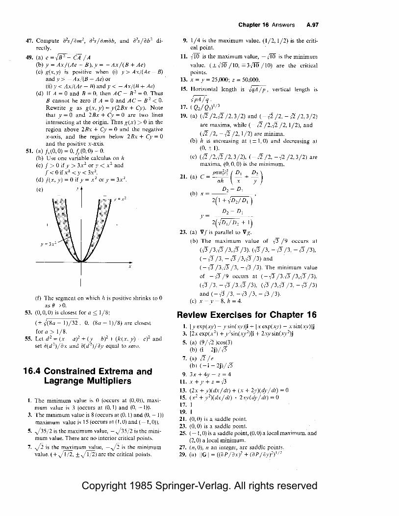
Copyright 1985 Springer-Verlag. All rights reserved
47. Compute il2s /ilm 2, il 2s /ilmilb, and il 2s /ilb 2 di
rectly.
49. (a) e=i/B 2- CA /A
(b) y = Ax/(Ae - B),y = -Ax/(B + Ae) (c) g(x,y) is positive when (i) y > Ax/(Ae - B)
and y > - Ax/(B + Ae) or (ii) y < Ax/(Ae - B) and y < -Ax/(B + Ae)
(d) If A= 0 and B = 0, then AC - B 2 = 0. Thus B cannot be zero if A = 0 and AC - B 2 < 0. Rewrite g as g(x, y) = y(2Bx + Cy). Note that y = 0 and 2Bx + Cy = 0 are two lines intersecting at the origin. Thus g(x) > 0 in the region above 2Bx + Cy = 0 and the negative x-axis, and the region below 2Bx + Cy= 0 and the positive x-axis.
51. (a) fx(O, 0) = 0, fy(O, 0) = 0. (b) Use one variable calculus on h (c) f > 0 if y > 3x2 or y < x 2 and
f < 0 if x 2 < y < 3x2.
(d) f(x, y) = 0 if y = x 2 or y = 3x 2.
(e) Y
y = x2
+
x
(f) The segment on which h is positive shrinks to 0 as 0---70.
53. (0, 0, 0) is closest for a _::::: 1/8;
(± V(8a - 1)/32, 0, (8a - 1)/8) are closest
for a> 1/8. 55. Let d 2 = (x - a)2 + (y - b)2 + (k(x, y) - c)2 and
set il(d 2)/ilx and il(d 2)/ily equal to zero.
16.4 Constrained Extrema and Lagrange Multipliers
I. The minimum value is 0 (occurs at (0,0)), maximum value is 3 (occurs at (0, 1) and (0, -1)).
3. The minimum value is 8 (occurs at (0, 1) and (0, -1)) maximum value is 15 (occurs at (1,0) and (-1,0)).
5. j35/2 is the maximum value, -j35/2 is the minimum value. There are no interior critical points.
7. fi is the maximum value, -fi is the mini.mum value. ( ± j172, ± j172) are the critical points.
Chapter 16 Answers A.97
9. I/ 4 is the maximum value. ( 1 /2, 1 /2) is the critical point.
11. fiO is the maximum value, - fiO is the minimum
value. (± fiO /10, +3/iO /10) are the critical points.
13. x = y = 25,000; z = 50,000.
15. Horizontal length is i/qA / p , vertical length 1s
VpA/q. 17. ( Q1/ Q1) 113
19. (a) CII /2,II /2,3/2) and (-II /2, -II /2,3/2)
are maxima, while ( - II /2,/2 /2, 1 /2), and
(II /2, - II /2, 1 /2) are minima. (b) h is increasing at ( ± 1, 0) and decreasing at
(0, ± 1).
(c) <II /2,II /2,3/2), (-II /2, -II /2,3/2) are maxima, (0, 0, 0) is the minimum.
21. (a) C = --1-
1 ~ + --2 P7Tn2i
2 ( D D )
ah x y
D2- D1 (b) x = ,
2( 1 + ,/ D 2/ D 1 )
D2- D1 y=------
2(./D1/ D 2 + 1) 23. (a) V f is parallel to V g.
(b) The maximum value of ff /9 occurs at
(ff /3,ff /3,ff /3), (ff /3, -ff /3, -ff /3),
( - ff /3, -ff /3,ff /3) and
(-ff /3,ff /3, - ff /3). The minimum value
of - ff /9 occurs at ( - ff /3, ff /3, ff /3),
(ff /3, -ff /3,ff /3), (ff /3,ff /3, -ff /3)
and ( - ff /3, - ff /3, - ff /3). (c) x = y = 8, h = 4.
Review Exercises for Chapter 16 1. [y exp(xy) - y sin(xy))i + [x exp(xy) - x sin(xy)Jj 3. [2x exp(x 2
) + y 2sin(xy 2))i + 2xy sin(xy2)j
5. (a) (9/II)cos(3) (b) (i - 2j) / v'5
7. (a) II/ e (b) (-i - 2j)/y's
9. 3x + 4y - z = 4 11.x+y+z=ff
13. (2x + y)(dx/ dt) + (x + 2y)(dy / dt) = 0 15. (x 2 + y2)(dx / dt) + 2xy(dy / dt) = 0 17. 1 19. 1 21. (0, 0) is a saddle point. 23. (0, 0) is a saddle point. 25. ( - 1, 0) is a saddle point, (0, 0) a local maximum, and
(2, 0) a local minimum. 27. (n, 0), n an integer, are saddle points. 29. (a) llGll = ((ilP /ilx)2 + (ilP /ily)2
)112

Copyright 1985 Springer-Verlag. All rights reserved
A.98 Chapter 16 Answers
(b) According to Newton's second law of motion, G creates a force on the air mass which produces a proportionate acceleration in the direction of G.
(c)
North
Y low
m\pressure
~ hh ~ p~!ssure
@jD wind
(d) If, in the Southern Hemisphere, you stand with your back to the wind, the high pressure is on your left and the low pressure is on your right.
North
high pressure
low
~ pressure
([) wind
31. (a) ( ± I, 0, 0) are closest, distance is I.
(b) (-/<IT /6,/<IT /6, 1/6),
(/<IT /6, -[<IT /6, 1/6) are closest,
the distance is m /6.
x
( c) ( - I, - I, I), ( - I, I, - I), (I, - I, - I) and
(I, I, I) are closest, the distance is /3. 33. 0.382 is the minimum value, 2.618 is the maximum
value. 35. 0.540 is the minimum value, I is the maximum
value. 37. The partials of k(x, y, A.)= x + 2y sec B +
A.(xy + y 2tan B - A) must all vanish 39. (a) Use the second derivative test.
(b) Since the maximum and minimum must occur on the boundary (by (a)), both are zero. Hence f is everywhere zero.
41. (a)(!, 1,2), x + y + 2z = 6; (2,3,2), 2x + 3y + 2z = 9.
(b) B = 0.47 (c) (!, 1, 2) + t(-4, 2, I)
43. (a) A normal vector to the tangent plane is j) + fyj - k.
(b) The slope of the plane relative to the -".Y plane
is 5; the plane contains the line through the point (I, 0, 2) parallel to the y-axis.
45. Equate the four partial derivatives equal to zero. Eliminate A. 1 by subtracting two equations and A.2 by dividing two equations.
47. 600 49. Approximately 570 51. (4, 2) 53. (a) dy / dx = -(2x)/(3y2 + eY)
(b)
d Id _ (aF1/a12)(aF2/ax) - (aFifa12)(aF1/ax)
!JI X - -;-;c-c;:o--~--,-c~-::-;~-c-----:-::-=--ccc-----,.---c--( a F2 /a J2) (a F 1 /a y I) - (aF2/ay1)(aF1/a12)
I (aF1/ay1)(aF2/ax) - (aF1/ax)(aF2/av1) dJ2 dx = -c::---=---~--:-c-::---:-cc-~--------
( aF1/a12)(a F2/a y1) - (aFifa12)(aF1/ay1) (c) dy 1/dx = -(2x + sinx)/2y 1,
d12/ dx = (cosx - 2x)/J2. 55. (a) Use equality of mixed partials of j(x, y)
(b) Use equality of mixed partials of j(x, y,z) (c) No
57. (a) x 2exp(xy2) + C (b) No function exists. (c) In(!+ x 2 + y 2
) + C. (d) No function exists.
59. (a) (x0 , - y 0)
(b) (yo, xo) (c) g(x, y) = xy ( d) Since V g is normal to the level curves of g, the
tangent to these curves is normal to level curves off.
(e)
y
f= corn;tant
x
61. (a) fx = - 2xy3 / (x2 + y2)2, fy = y2(3x2 + y2)/(x2 + y2)2. fx(O, 0) = 0 and fy(O, 0) = I (compute the latter two using limits).
(b) (a/ar)j(rcosB,rsinB) = cos2B( - 2 sin3B + 3 sin2B + I) is defined for all B.
(c) V j(O, 0) ·(cos B, sin B) =sin B disagrees with the formula in (b). There is no contradiction because the partial derivatives are not continuous at (0, 0) (see Exercise 20, p; 783).

Copyright 1985 Springer-Verlag. All rights reserved
Chapter 17 Answers 17 .1 The Double Integral and
Iterated Integral 1. 12 3. (a) Divide D into D 1 = [ - 1, O] x [2, 3],
D2 = [-1,0] X (3,4], and D3 = (0, l] x [2,4]. Let g(x, y) be -4 on D 1, -5 on D2 , and O on D3.
(b) The part of the integral for x .;; 0 is the negative of the part for x -;, 0.
z
x
5. 18 7. 16/9 9. e/2 - 1/2e
11. 50 13. 4/3 is. 45 / 4 + (15 /2)In(3 /2)
y
17. O; this agrees with the answer in Exercise 3(b).
19. 76/3
x
y
Chapter 17 Answers A.99
21. 25/6 grams. 23. Use partition points obtained from subrectangles
for both the functions being added. 25. (a) 0.88[ 1 - sin2o: cos2(2'1TT /365)] 112cos(27rt /24)]
+ 0.67 sin o: cos(2'1TT /365), where o: = 23.5° (b) This is the total solar energy received in the
state between times t 1 and t2 on day T.
17 .2 The Double Integral Over General Regions
1. Both a type 1 and a type 2 region.
y
3
x
3. Both a type 1 and a type 2 region.
-1
5. 7 /12
y
1
-1
9. Type I; 2'1T + 'IT2
y
3
" x
7. 64/35
x

Copyright 1985 Springer-Verlag. All rights reserved
A.100 Chapter 17 Answers
11. Type 2; 104/45
y
-]
-]
13. fype 1; 33/140
y
15. Type I; 71/420
y
0
17. 1/8
y
19.7/12
y
21. I /3 23. 19/3
x
x
x
x
x
25. The result of the first integration is the length of a section of the region.
27. Type 1 states include: Wyoming, Colorado, Nevada, New Mexico,. Kansas, and Ohio. Type 2 states include: Wyoming, Colorado, Kansas, North Dakota, and Vermont.
17 .3 Applications of the Double Integral
1. 12'7T 3. (4/5)(2 + 9\/4) 5. 10 + 8/n
(3,2,0)
x
y (1, 2,0)
9. 243/80 13. 2
7. (16e2 - 16 + '7T 4)/32
11. [ '7T 2 - sin( ?T
2)]/ ?T
3
15. 2/3 19. (11/18,65/126)
17. 2a2 /3 21. (7 /5, 0)
23. (4/15)(9,13 - 8/I + l) 25. II '7T/4
27. Compare the formulas for average value and center of mass.
29. (a) Write z = ± ~r1 - x 1
- y2 over the region
0 < x < r, - Jr1 - x 1 < y < Jr1
- x1 .
(b) The result is independent of r. 31. $503.64
33. 2 (hJJ(x) V[f(x)]2 - y 1 dydx = '7T fU<x)]2dx.
Ja - /(x) a (This is the disk method; see p. 423.)
17 .4 Triple Integrals 1. 7 7. Type I
13. 0
19. 3/10
3. -8
9. 25J2/3 '7T 15. a 5 /20
5. Type I 11. I /2 17. 0
21. The double integral of F over the base of the box times the height of the box.
23. Interchange x and z in Example 4. 25. The region under the graph is of type I. 27. (a) Use iterated integrals and the constant multi
ple rule for definite integrals. (b) ex+y+z = exeyez.

Copyright 1985 Springer-Verlag. All rights reserved
17.5 Integrals in Polar, Cylindrical, and Spherical Coordinates
1. 64'17 /5
3. v'17 ;10
5. 128'17 7. 5?7(e4
- 1)/2
9. 2'17[J2 - In(! +J2)J 11. 4'17 In( a/ b)
13. (?7/6)(8-3y'3) 15. 4'17{6
17. 1/{iia 19. (a) Use the linear approximations
ax ax ay ay D.x ~-a D.u + -a D.v and D.y ~ - D.u + - D.v.
u v au av
(b) Use the fact that I a(x. y) I= r. a( r. B)
21. The conditions 0 < y < I - x and 0 < x < I are
equivalent to 0 < x + y < I and O < _Y_ < I. x+y
v
17 .6 Applications of Triple Integration
1. (a) p, where p is the (constant) mass density. (b) 41/3
·3, (1/2. 1/2. 1/2)
5. ~ (as in Example 2)
7. (a) kc 2
(b) Along the sphere x 2 + y 2 + z 2 = c2
9. 1/4
II
11. Letiing d be density, the moment of inertia 1s d fokfo2" foasec<f>p4sin3<j>dpd8d<j>
13. 1.00 X 10⁸(m/s)2
15. (a) The only plane of symmetry for the body of an automobile is the one dividing the left and right sides of the car.
(b) z · J J fwp(x, y,z)dx dy dz is the z-coordinate
of the center of mass times the mass of W.
Chapter 17 Answers A.101
Rearrangement of the formula for z gives the first line of the equation. The next step is justified by the additivity property of integrals (see rule 2 on p. 841). By symmetry, we can replace z by - z and integrate in the region above the xy-plane. Finally, we can factor the minus sign outside the second integral and since p(x, y, z) = p(u, v, - w), we are subtracting the second integral from itself. Thus, the answer is 0.
(c) In part (b), we showed that z times the mass of W is 0. Since the mass must be positive, z must be 0.
(d) By part (c), the center of mass must lie in both planes.
17. Follow the pattern on p. 880 for the case of constant density. Be sure to use different symbols for the density and the spherical coordinate
~x2 + y2 + z2.
Review Exercises for Chapter 17
1. 960 - sin(! I) + sin( 10) + sin(7) - sin(6) ~ 961.4 3. 15/2 5. 64/3 7. '17 in(sec I +tan I) 9. 1/48
11. 10/3 13. 4?7abc/3
15. 2'17(1 - !/va+J)/3
17. (25 + IOVS)?7/3
19. (4'17 /3)(1 -v'2 /2) 21. 40'17 /3
( -3. 7T. 10)
( -3.1T, 0)
(l, 1T.0)
23. 10/3 25. Cut with the planes x + y + z = 3 ,/k/n,
I < k < n - !, k an integer. 27. Use the formula for surface area.

Copyright 1985 Springer-Verlag. All rights reserved
A.102 Chapter 18 Answers
29. (0, 0, - 0.203)
31. 27T(2/I - 1)/3
33. 7T(5{5 - 1)/6 35. 7T2 /8 37. c 7T / 4)ln(2) 39. V(O, 0, R) = (4.71 x 10²²)G/ R 41. (a) 32/3
(b) 647T
43. J7T /5 45. (a) It is equal to the average of the values of the
function at the vertices.
Chapter 18 Answers 18.1 Line Integrals
1. 5 7. -27T
13. 27T2
19. 2 + e
23. 2/3 27. (cos3)/3 + 5/12 31. (5{5 - 1)/12
3. 0 9. 7T
15. - I
21. I 25. -1/2 29. 0 33. 52/f4
5. 3/2 11. 27T 17. 0
35. Use the chain rule and make a change of variables in the integral.
18.2 Path Independence 1. 3 3. 8 5. 1 /2 7. 7T 9. 0 11. 256
13. JMm(r2-3
- r;- 3)/3 17. Yes; xy +sin y + C 15. No 19. Yes; x 2 + x 2cos y + C
21. Calculate fx = - y /(x2 + y 2) and
fy = x/(x2 + y2). 23. 27T2
25. 0 27. (a) The integrals along the four sides are 0, I, - 1,
and 0. (b) j(x, y, z) = z 3x + xy + C.
29. (I /2)3 - (/I /2)3 + sin(3/I 7T / 4)
31. The field is not conservative. 33. x exp(yz) + C 35. If "ii f ="ii g then "ii (j - g) = 0. Show that f - g is
constant, using the second box on p. 896. 37. Pick a point P and draw an arc from P to each
region. If the arc crosses the circles an even number of times, color the region red, otherwise color the region blue.
18.3 Exact Differentials 1. No 3. No 5. Not exact 7. Exact 9. J is the integral of P dx + Q dy along the line
segment from (0, 0) to (0, y) followed by the segment from (0, y) to (x, y).
(b) Same as in (a). 47. Using d for density, the potential is given by
27TdG[(P2)2 - R 2 /3 - 2(p 1)3 /3R].
49. Show that the double integral of fxy - hx over every rectangle is zero.
51. u; + u} =I
11. The two line integrals are equal since P dx + Q dy is exact.
13. xeY + yex = 2 15. x 3 + xy + y 3 /3 = 17 /3. 17. Not exact 19. 2x 3y + x 2y 2 = C 21. (a) - I
(b) y = x 23. y = ±x 25. fl= x 27. x 2/2 + x/y = C
29. In fl= f [CNx - My)/ M]dy
31. If f is an antiderivative of P dx + Q dy, then
fx = aax J p dx; now integrate.
18.4 Green's Theorem 1. Each side gives I/ 12. 3. Each side gives - 7T.
5.
y
7.
y
x
x

Copyright 1985 Springer-Verlag. All rights reserved
9. -4Jb ((a/b) b'-y' xydxdy = 0 -b)(a/b) b2 -y2
11. 67 /6 13. -20 15. 0 17. (a) Recall that a zero dot product implies orthogo
nality. (b) Use Green's Theorem.
19. In applying the hint, note that the terms involving Vu· Vv cancel.
21. 9
23. Simplify A= t fcxdy - ydx to
3a2
(2
"' sin22(} dB; now use the double angle for-8 Jo
mula to integrate. 25. 5/12 27. A horizontal line segment divides the region into
three regions to which Green's theorem applies; see Example 2.
29. 0 31. aa;ay = Q by the r iamental theorem of calcu-
lus; similarly for :> , JX = P. 33. The device is run around the perimeter of the
region and the mechanism evaluates the integral
_!_ ( (xdy - ydx). 2 JaD
18.5 Circulation and Stokes' Theorem
1. -2 3. 4xy /(x 2 + y 2)2 5. 8 7. 0 9. z 3i + e'j + (y sin xy)k.
11. (2/(x 2 + y 2 + z 2)2)(x 3i + (xy - yz 2)j - z 3k)
13. Let <I>= Pi+ Qj + Rk, write out curl (j<I>), and use the product rule for derivatives.
15. V XV J = 0 is a vector identity; the integral of an exact differential about a closed loop is zero.
17. Compute that V X <I>= 0 and use Stokes' theorem. 19. -1/2
21. Use Stokes' theorem and <l>(u(s)) · u'(s) = 0. 23. - 17'lr/2
25. fcH(r) · dr = J fscv xH) · ndA = J fsJ · ndA
27. The component of the curl of the velocity of the fluid along a vector n is the circulation around n per unit area (p. 921); this is maximized when the curl and n are aligned.
29. Partition the surface into the upper and lower hemispherical pieces; apply Stokes' theorem to each piece and add.
Chapter 18 Answers
18.6 Flux and the Divergence Theorem
1. 3x2 - x 2cos(xy) 3. y cos(xy) - x 2sin(x2 y) 5. -4 7. 0 9. (a) A,C
(b) B,D 11. y exp(xy) - x exp(xy) + y exp(yz) 13. 3 15. !2'lr /5 17. I 19. Use Gauss' theorem and V · n = 0. 21. Apply the divergence theorem to f<I> using
V ·(j<I>) =VJ· <I>+ JV ·<I>. 23. (i) Use the vector identity V · (V X H) = 0.
A.103
(ii) Since charge is conserved, the rate at which charge is entering equals the rate at which charge is leaving; the total flux is therefore zero. By Gauss' theorem, the integral of V ·J over any region is zero, so V ·J = 0.
25. (a) Calculate div Vcp on a region excluding a small ball near q.
(b) Use (a).
Review Exercises for Chapter 18
1. !0/3-2cos2+2sin2-2sinl 3. 2e 5. -8 7. I - e 9. -cos5 + cos3 + (ln4)2/4+ (44ln2)/3 + 83/18
11. (a) sin(ln(5/4))- sin(ln(3/4))- (In(5/4))2 + (In(3 / 4))2
(b) 0 (c) 0
13. 43/54 15. - 1 17. (e - 1)/3 19. Not conservative 21. Not conservative 23. Yes; 3zy + xy + C 25. Exact; xeYsin x + C 27. Not exact 29. ysinx + x 2eY + 2y = 7r
2 /4 31. -x + xy + y = I 33. Not exact 35. Not exact
37. (a) J L (I) dx dy, the area of D
(b) J L(-l)dydx, the negative of the area of D
(c) J L (O)dydx = 0
39. curl <I>= [y /(x + z)2]i - [y /(x + z)2]k; div<I> = 1/(x + z)
41. curl <I>= -4xi - 2yj + 2zk; div <I>= 0.

Copyright 1985 Springer-Verlag. All rights reserved
IU04 Chapter 18 Answers
43. (a) V XF = 2x 3yzi- 3xy2zj + 2k, V·F = x}i2 (b) 27T (c) 1/12
45. J fs(V xF) • ndA, where C is the boundary of S.
47. 0 49. -27T /3 51. Use Gauss' theorem. 53. Use Gauss' theorem over a small region; divide by
the volume of the region and use the mean value theorem for integrals.
55. -87T
57. (a) Letu'= foxa(t,O,O)dt+ fo 2
c(x,O,t)dt+
foyb(x, t, z)dt, so au' jay= Q. Permute x, y, z
to give u" with au" /az = R, and u"' with au'" /ax= P. Use Stokes' theorem to show that u' = u" = u"'.
(b) xyz - cosx + C
59. J faj(VJ)-ndA = J J fw(f'il 2J +VJ· VJ)dxdydz
gives 0 = J J fw(VJ· Vf)dxdydz
= J J f)VJll 2 dxdydz, so VJ= 0 and thus
J is constant.
61. J fs (V X <I>) • ndA = 0 if S is the union of the two
surfaces.

Copyright 1985 Springer-Verlag. All rights reserved
Index Includes Volumes I, II and Ill
Note: Pages 1-336 are in Volume I; pages 337-644 are in Volume II; pages 645-934 are in Volume III.
Abbot, Edwin A. 883 Abel, Nils Hendrik 172 absolute value 22
function 42, 72 properties of 23
absolutely convergent 574 accelerating 160 acceleration 102, 131 , 7 41
gravitational 446 vector 741
Achilles and tortoise 568 addition formulas 259 addition of ordered pairs 646 air resistance 136 Airy's equation 640 algebraic
operations on power series 591 rules 16
alternating series test 573 amplitude 372 analytic 600 angular
frequency 373 momentum 506, 748
annual percentage rate 382 antiderivative 104, 128, 897
of Ir 323, 342 of constant mutiple 130, 338 of exponential 342 of hyperbolic functions 389 of inverse trigonometric function 341 of Ilx 323, 342 of polynomial 130
of power 130, 338 rules 337, 338 of sum 130, 338 of trigonometric function 340 of trigonometric functions 269
Apollonius 696 Apostol, Tom M. 582 approaches 58 approximation
first-order (see linear approximation) linear (see linear approximation)
arc length 477 of curve in space 745 parametrized by 749 in polar coordinates 500
Archimedes 3,5,6 area 4, 251
between curves 853 between graphs 211, 241 between intersecting graphs 242 of graph 857 of n-sided polygon 934 of parallelogram 683 in polar coordinates 502 of region bounded by a curve
914 of sector 252 of surface 482 of revolution 483 signed 215 of triangle 934 under graph 208, 212, 229
of step function 210

Copyright 1985 Springer-Verlag. All rights reserved
1.2 Index
argument 40 arithmetic mean 188 arithmetic-geometric mean inequality 436 associative 679 astigmatism 821 astroid 198 astronomy 9 asymptote 165
horizontal 165, 513, 535 of hyperbola 698 vertical 164, 518, 531
asymptotic 164 average 3
power 464, 465 rate of change 100 value 434, 854, 878 velocity 50 weighted 437
axes 29 rotation of 705, 707 translation of 703
axial symmetry 423 axis
major 696 minor 696 of symmetry 440
B-o definition of limit 516 ball 421 Bascom, Willard 306(fn) base of logarithm 313 basis vectors, standard 656 bearing 659 beats 628 Beckman, P. 251, (fn) Berkeley, Bishop George 6(fn) Bernoulli, J. 252(fn), 521
equation 414 numbers 643
Bessel, F.W. 639 equation 639 functions 643
Binder, S. M. 836 binomial series 600 binormal vector 753 bird 692 bisection, method of 142, 145 blows up 399 Boltzmann's constant 823 bouncing ball 549 boundary 848, 908 bounded above 575 Boyce, W. 401 Boyer, C. 7(fn), 252(fn) Braun, Martin 380, 401, 414, 626 Burton, Robert 8 bus, motion of 49, 202, 207, 225
Buys-Ballot's law 834
Calculator discussion 49, 112, 166, 255, 257, 265, 277, 309, 327, 330, 541
calculator symbol 29 Calculus Unlimited iii, 7(fn) calculus
differential 1 fundamental theorem of 4, 225, 237 integral 1,3
Calder, Nigel 756 capacitor equation 406 Captain Astro 802, 804, 816 carbon-14 383 Cardano, Girolamo 172 cardiac vector 658 cardioid 298 cartesian coordinates 255 catastrophe
cusp 176 theory 176
catenary 402 Cauchy, Augustin-Louis 6, 521, 908
mean value theorem 526 Cauchy-Riemann equations 835 Cauchy-Schwarz-Buniakowski
inequality 669 Cavalieri, Bonaventura 8, 425
principle 843 center of mass 437, 693, 857, 876
in the plane 439 of region under graph 441 of triangular region 445
centripetal force 747 chain rule 112, 779
for partial derivatives 800 physical model 116
change average rate of 100 instantaneous rate of 10 linear or proportional 100 proportional 95 rate of 2, 100, 101, 247 of sign 146 total 244 of variables 877
chaos and Newton's method 547 characteristic equation 617 charge 930 chemical equation 648, 651, 660 chemical reaction rates 407 circle 34, 44, 120, 251, 421
as section of cone 695 equations of 37 parametric equations of 490
circuit, electric 413 circular functions 385

Copyright 1985 Springer-Verlag. All rights reserved
circulation 914 circumference 251 city
Fat 116 Thin 115
Clairaut 767 climate 180 closed curve 889 closed interval 21 closed interval test 181 closed rectangle 839 Cobb-Douglas production function 831 College, George 383 common sense 61, 193 commutative 788 comparison test 570
for improper integrals 530 for limits 518 for sequences 543
completing the square 16, 17, 463 complex number 607, 609
argument of 609 conjugate of 609 imaginary part of 609 length or absolute value of 609 polar representation of 612 properties of 610 real part of 609
component 648 functions 738
composition of functions 112, 113, 779 compressing fluid 926 computer-generated graph 716, 717, 720,
721, 813, 819, 821, 822, 833, 834, 837
concave downward 158 upward 158
concavity, second derivative test for 159 conditionally convergent 574 cone, elliptic 728, 793 conic sections 695 connected 897 conoid 486 conservation of energy 372 conservative vector field 895 consolidation principle 438 constant function 41, 192
derivative of 54 rule for antiderivatives 130 rule for derivatives 77 rule for limits 62, 511 rule for series 566
constrained extrema 825 first derivative test for 826
consumer's surplus 248 continuity 63, 72, 770
equation 953
Index 1.3
of rational functions 140 continuous function 63, 139, 770
integrability of 219 continuously compounded interest 3 31 ,
382, 416 convergence
absolute 574 conditional 574 radius of 587 of series 562 of Taylor series 597
convergent integral 529 convex function 199 cooling, Newton's law of 378 Cooper, Henry S. Jr. 682 coordinates 29, 648, 653
cartesian 255 polar 253, 255, 791, 869 spherical 731
Coriolis force 499 cosecant 256
inverse 285 cosine 254
derivative of 266 direction 676 hyperbolic 385 inverse 283 law of 258, 676 series for 600
cost, marginal 106 cotangent 256
inverse 285 Coulomb's law 805 Cramer, Gabriel 690
rule 690 Creese, T.M. 401 critical points 151, 814 critically damped 621 cross product 674, 679, 754 cross-derivative test 898, 904 Crowe, M. J. 657 cubic function 168
general, roots and graphing 172 curl
of a vector field 917 scalar 915
curvature 749, 750, 821 curve 31
closed 889 geometric 889 level 712 parametric 124, 298, 489
in space 735 regular 749 in space, arc length of 745
cusp 170 catastrophe 176
cycloid 497

Copyright 1985 Springer-Verlag. All rights reserved
1.4 Index
cylinder 715, 722 parabolic 714, 723
cylindrical coordinates 728 triple integrals in 872
dam 454 damping 377
in forced oscillations 626 in simple harmonic motion 415
Davis, Phillip 550 day
length of 30, 302 shortening of 303 sidereal 757 solar 757
decay 378 decelerating 160 decimal approximations 538 decrease, rate of 101 decreasing function 146 definite integral 232
constant multiple rule for 339 endpoint additivity rule for 339 inequality rule for 339 power rule 339 properties of 234, 339 by substitution 355 sum rule for 339
degree as angular measure 252 of polynomial and rational functions 97
delicatessen, Cavalieri' s 425 delta 50(fn) demand curve 248 Demoivre, Abraham 614
formula 614 density 440
uniform 440 dependent, linearly 89 depreciation 109 derivative 3, 53, 70
of Ir 318 of composition 113 of constant multiple 77 of cosine 266 of hyperbolic functions 388 of implicitly defined function 122 of integer power 87 of integral with respect to endpoint 236 of integral, endpoint a given
function 236 of inverse function 278 of inverse hyperbolic function 396 of inverse trigonometric functions 285 of linear function 54 of logarithmic function 321 of llx 71
of polynomial 75, 79 of power 75, 119
of a function 110, 119 of product 82 of quadratic function 54 of quotient 85 of rational power 119
of a function 119 of reciprocal 85 of sum 78 of vector function 739 of Yx71 as a limit 69 directional 801 formal definition of 70 Leibniz notation for 73 logarithmic 117, 322, 329 matrix 784, 786 partial 765 second 99, 104, 157 second partial 768 summary of rules 88
determinant 683, 685 jacobian 792
Dido 182 Dieterici's equation 795 difference quotient 53, 766 differentiable 70 differential
algebra 356 calculus 1 equation 369
Airy's 369 Bessel's 639 Euler's 796 first order 3 69 of growth and decay 379 harmonic oscillator 370 Hermite's 636 Legendre's 635 linear first order 369 of motion 369 numerical methods for 405 partial 898 second-order 399 second-order linear 617 separable 398, 399 series solution of 632 solution of 369 spring 370 Tchebycheff's, 640
form 893, 902 geometry 749 notation 351, 359, 374, 398
differentiation 3, 53, 122, 201 implicit 120, 398, 810 logarithmic 117, 322, 329 partial 767

Copyright 1985 Springer-Verlag. All rights reserved
of power series 590 rules for vector functions 740 under integral sign 883
diminishing returns, law of 106 dipole 693 Diprima, Richard 390, 401 direction
angles 676 cosines 676 field 403
directional derivative 80 l directrix 700 discriminant 17 disk 421
method 423 displacement 230
vector 657 distance formula
in the plane 30 on the line 23
divergence 925 free 926 theorem 694, 924
divergent integral 529 dog saddle 722 domain 41 dot product 668 double integral 839, 850
applications of 853 over general regions 847 in polar coordinates 870 properties of 841
double-angle formulas 259 drag 136, 414 dummy index 203
e 319, 325 as a limit 330
e-A definition of limit 513 e-8 definition of limit 511, 769 ear popping 116 earth, rotation of 756 earth's axis, inclination of 30 l eccentricity 702 economics 105, 830 electric circuits 399, 413 element 21 elementary regions 848, 864 ellipse 696
equation of 696 focus of 696 reflection of property of 702 as section of cone 695 shifted 703
ellipsoid 724, 793 elliptic
cone 728, 273
Index 1.5
hyperboloid of one sheet 760 integral 417, 506, 507 paraboloid 728
endpoints 181 of integration 217
energy 201, 445 conservation of 372 equation 753 potential 446
equation chemical 648, 651, 652, 660 differential 369 (see also differential
equation) indicial 638 of circle and parabola 3 7 of ellipse 696 of hyperbola 698 of line 662 of parabola 701 of plane 671 of plane in space 672 of straight line 32 of tangent line 90 parametric 124, 298 simultaneous, 37 spring 376
equipotential surfaces 816 error function 558 Eudoxus 4 Euler, Leonhard 25l(fn), 252(fn), 369
differential equation 796 equation 636 formula 608 method 404
evaluating 40 even function 164, 175 exact differential 901 , 903 exhaustion, method of 5, 7 existence theorem 180, 219 expansion by minors 687 exponent zero 23 exponential and logarithmic functions,
graphing problems 236 exponential functions 307
derivative of 320 limiting behavior of 328
exponential growth 332 exponential series 600 exponential spiral 310, 333, 751 exponentiation 23 exponents
integer 23 laws of 25 negative 26 rational 27, 118 real, 308
extended product rule for limits 62 extended sum rule for limits 62, 69

Copyright 1985 Springer-Verlag. All rights reserved
1.6 Index
extensive quantity 445 extreme value theorem 180 extremum, local 813
factoring 16 falling object 412, 414 Faraday's law 922 Feigenbaum, M. J. 548 Feinberg, M. 836 Ferguson, Helaman 602 Fermat, Pierre de 8 Fine, H.B. 468 first derivative test 153, 814
for constrained extrema 826 first-order approximation (see linear
approximation) Fisher, Chris 884 fluid 914, 926 flux 924
law 805 of a vector field 925
flying saucer 430 focus of ellipse 696 focusing property of parabolas 36, 95, 97,
701 football 453 force 448, 659, 675, 885, 886
centripetal 747 on a dam 454 gravitational 834 resultant 659
forced oscillations 415, 624 four-petaled rose 730 Fourier coefficients 506 fractals 499 fractional exponents (see rational
exponents) fractional powers (see rational powers) Frenet formulas 753 frequency 259 friction 3 77 Friedrichs, Kurt 694 Frobenius, George 636 frustrum 485 function 1, 39
absolute value 42, 72, 73 average value of 434 circular 385 component 738 composition of 112, 113, 779 constant 41, 192 continuous 63 convex 199 cubic 168 definition of 41 differentiation of 268 even 164, 175
exponential 307 graph of 41, 44 greatest integer 224 harmonic 774 homogeneous 796 hyperbolic 384, 385 identity 40, 277, 384, 385 integration of 217 inverse 272, 274 inverse hyperbolic 392 inverse trigonometric 281, 285 linear 192 odd 164, 175 piecewise linear 480 power 307 rational 63 squaring 41 step 140, 209, 210, 839, 861 of three variables 712 trigonometric, antiderivative of 269 trigonometric, graphs of 260 of two variables 711 vector 737 zero 41
fundamental integration method 226 fundamental set 630 fundamental theorem of calculus 4, 225,
237 alternative version of 236
Galileo 8 gamma function 643 gas
ideal 795 Van der Waals 795
Gauss, Carl Friedrich 205, 613, 908 divergence theorem in the plane 925 in space 927
gaussian integral 870, 871 Gear, C. W. 405 Gelbaum, Bernard R. 576, 600 general solution 618, 623 geometric curve 889 geometric mean 188, 436 geometric series 564, 600 geometry, differential 749 Gibbs, J. Willard 657 global 141, 177
maximum 813 Goldman, M. J. 658 Goldstein, Larry 172 Gould, S.H. 6(fn) gradient 197, 798
and Laplacian in polar coordinates 836 and level curves 808 pressure 833 and tangent planes 806

Copyright 1985 Springer-Verlag. All rights reserved
vector fields 896 graph 41, 163
area between 241 area under 212, 229 computer-generated 716, 717, 720, 721,
813, 819, 821, 822, 833, 834, 837 of function 41, 44
of two variables 711 surface area of 857
graphing in polar coordinates 296 graphing problems
exponential and logarithmic functions 236
trigonometric functions 292 graphing procedure 163 gravitational acceleration 446 gravitational force 834
inside a hollow planet 880 gravitational potential 878, 882, 883 greatest integer function 224 Green, George 908
identities 933 theorem 908, 911
growth 378 and decay equation, solution of 379 exponential 332
gyroscope 682
half-life 381, 383 hanging cable 401 Haralick, R.M. 401 Hardin, Garrett 416 harmonic series 567 harmonic function 774 heat
conduction 772 equation 775, 933 flow 933
helix, right circular 736 Henderson, James 831 Hermite polynomial 636 Hermite's equation 636 herring 156 Hipparchus 256(fn) Hofstadter, Douglas 548 Holder condition 559 homogenous equation 623 homogenous function 796 Hooke's Law 99, 295 horizontal asymptote 165, 513, 535 horizontal tangent 193 horsepower 446 horserace theorem 193 hyperbola 698
asymptotes of 698 equation of 698 shifted 703
Index 1.7
hyperbolic cosine 385 hyperbolic functions 384, 385
antiderivatives of 389 derivatives of 388 inverse 392
hyperbolic paraboloid 719, 720, 728 hyperbolic sine 385
inverse of 393 hyperboloid
of one sheet 725 elliptic 7 60
of revolution 725 as ruled surface 763 of two sheets 724
I method 361 ice ages 756 ideal gas 795 identity function 40, 277
rule for limits 60 identity, trigonometric 257 illumination 183 imaginary axis 609 imaginary numbers 18 implicit differentiation 120, 122, 398, 810 implicit function theorem 810 improper integrals 528, 529
comparison test 530 inclination, of the earth's axis 301 incompressible 926 increase, rate of 101 increasing function 146
test 148 theorem 195
increasing on an interval 149 increasing sequence property 575 indefinite integral (see antiderivative)
test 233 independent variable 40 indeterminate form 521 index
dummy 203 substitution of 205
indices of refraction 682 indicial equation 638 induction, principle of 69 inequalities 18
properties of 19 inequality
arithmetic-geometric mean 188, 436 Cauchy-Schwarz-Buniakowski 669 Minkowski' s 365 Schwartz 669 triangle 665
infinite limit 66 infinite series 561 infinite sum 561

Copyright 1985 Springer-Verlag. All rights reserved
1.8 Index
infinitesimal 73 parallelograms 856
infinitesimals, method of 6, 8, 419, 428, 441, 477, 482, 495, 856, 872
infinity 21 inflection point 159
test for 160 initial conditions 371, 398 inner product 668 instantaneous quantity 445 instantaneous velocity 50, 51 integer power rule for derivatives 87 integers 15
sum of the first n 204 integrability of continuous function 219 integrable 217, 848, 861 integral 129, 217, 861
calculated "by hand" 212 calculus 1 convergent 529 definite 232 definition of 217 divergent 529 double 8-39, 850 elliptic 417 gaussian 870, 871 of hyperbolic function 389 improper 528, 529 indefinite 129 (see also antiderivative) of inverse function 362 iterated 842
reversing order of 851 Leibniz notation for 132 line 888, 893 mean value theorem for 239, 435 of rational expression in sin x and
cos x 475 of rational function 469 Riemann 220 sign 129, 132, 217
differentiation under 883 surface 916 tables 356 trigonometric 457, 458 triple 860, 861, 865 of unbounded function, 531 wrong way 235
integrand 129 integrating factor 905 integration 33, 129, 201, 851
applications of 420 by parts 358, 359 by substitution 347, 348, 352 endpoint of 217 limit of 217 method, fundamental 226 methods of 337 multiple 839
numerical 550 of power series 590
intensity of sunshine 451 interest, compound 244, 331 interior 839 intermediate value theorem 141, 14 2 intersecting graphs, area between 242 intersection of points 39 intertia, moment of 877 interval 21
closed 21 open 19
inverse cosecant 285 cosine 283 cotangent 285 function 272, 274
integral of 362 rule 278 test 276
hyperbolic functions 392 derivatives 396 integrals 396
hyperbolic sine 393 secant 285 sine 281 tangent 283 trigonometric functions 281, 285
invertibility, test for 275, 276 irrational numbers 16 isobars 833 isoquants 830 isotherms 710 iterated integrals 842
reduction to 843, 862 ith term test 567
Jacobi identity 682 Jacobian determinant 792 Jacobian matrix 792 joule 445
Kadanoff, Leo 548 Katz, V.J. 908 Kazdan, Jerry 716 Keisler, H. J. 7(fn), 73(fn) Kelvin, Lord 594, 908 Kendrew, W.G. 180 Kepler, Johannes 8
first law 753 second law 506
kilowatt-hour 446 kinetic energy 446, 859, 886 Kline, Morris 182 Korteweg--de Vries equation 783

Copyright 1985 Springer-Verlag. All rights reserved
I'Hopital, Guillaume 521 l'Hopital's rule 522, 523, 525 labor 106 ladder 190 Lagrange
interpolation polynomial 556 multiplier 826, 827
Laguerre functions 640 Lambert, Johann Heinrich 251(fn) Laplace equation 796 Laplacian 933 latitude 300, 732 least squares 823 Legendre, Adrien Marie 251(fn)
equation 635 polynomials 635
Leibniz, Gottfried 3, 73, 193, 594 notation 73, 104, 132, 217
for derivative 73 for integral 132
lemniscate 136 length
of curves 4 77 of days 300, 302 of parametric curve 495 properties of 665 of vector
level curve 712, 808 level surface 713 librations 506 lima<;:on 298 limit 6, 57, 59
comparison test 518 of (cos x - l)/x 265 derivative as a 69 derived properties of 62 c-3 definition of 509, 769 of functions 509 infinite 66 at infinity 65, 512 of integration 217 method 6 one-sided 65, 517 of powers 542 product rule 511 properties of 60, 511 reciprocal rule 511 of sequences 537, 540
properties of 563 of (sin x)lx 265
line 31(fn) equation of 32 integral 886, 893
of a scalar function 895 parametric equation of 664, 665 perpendicular 33 point-point form of 32 point-slope form of 32
real number 18 secant 51, 191 slope of 52 slope-intercept form 32 straight 31(fn), 125 tangent 2, 191, 741
Index 1.9
linear approximation 90, 91, 92, 158, 159, 601, 775, 776
linear combination 675 linear function 192
derivative of 54 linear or proportional change 100 linearized oscillations 3 7 5 linearly dependent 652, 689 linearly independent 652 Lipschitz condition 559 Lissajous figure 507 local 141, 151, 177
extremum 813 maximum point 151, 157 minimum point 151, 157, 813
logarithm 313 base of 313 defined as integral 326 and exponential functions, word
problems 326 function, derivative of 321 laws of 314 limiting behavior of 328 natural 319 properties of 314 series for 600
logarithmic differentiation 117, 322, 329 logarithmic spiral 534, 535 logistic equation 506 logistic law 407 logistic model for population 335 longitude 732 Lotka-Voltera model 400 love bugs 535 lower sum 210, 840, 861 Lucan 8(fn)
Maclaurin, Colin 594, 690 polynomials for sin x 602 series 594, 596
MACSYMA 465 magnetic field 752 major axis 696 majorize 199 Mandelbrot, Benoit 499 marginal
cost 106 productivity 106 profit 106 revenue 106

Copyright 1985 Springer-Verlag. All rights reserved
1.10 Index
Marsden, Jerrold 582, 615, 710, 810, 826, 849
mass action, law of 476 matrix 685, 784
derivative 784, 786 multiplication 787
Matsuoka, Y. 582 Mauna Loa 804 maxima and minima, tests for 153, 157,
181, 816 maximum
global 177 point 813 value 177
. . . max1mum-mm1mum
problems 177 test for quadratic functions 816
Maxwell equations 922, 923, 931 mean value theorem 191, 922
Cauchy's 526 consequences of 192 for integrals 239, 435, 455
Meech, L.W. 9 midnight sun 301(fn) minimum
points 177 local 813
value 177 Minkowski's inequality 365 minor axis 696 minors, expansion by 687 mixed partial derivatives 769 mixing problem 413, 414 modulate 628 moment
of a force 682 of inertia 878
momentum 692 monkey saddle 719, 721 motion, simple harmonic 373
with damping 415 multiple integration 839 multiplication
matrix 787 of ordered pairs 646
multiplier, Lagrange 826
natural growth or decay 380 logarithms 319 numbers 15
Newton, Isaac 3(fn), 8(fn), 193(fn), 253(fn), 594
iteration 559 law of cooling 378 law of gravitation 746 method 537, 546
accuracy of 559 and chaos 547
second law of motion 369, 746, 886 nonhomogenous equation 623 noon 30l(fn) normal 669
vector 671 principal 750
normalization 666 northern hemisphere 301 notation
differential 351, 359, 374, 398 Leibniz 73, 104, 132, 217 summation 203, 204
nowhere differentiable continuous function 578
number complex 607, 609 imaginary 18 irrational 16 natural 15 rational 15 real 15, 16
numerical integration 550
odd function 164, 175 Olmsted, J. M. H. 578, 600 one-sided limit 65, 517 open interval 21 open rectangle 839 optical focusing property of parabolas 36,
95, 97,701 orbit 702 order 18 ordered pairs
addition of 646 multiplication of 646
ordered triples, algebra of 654 orientation 683 orientation quizzes 13 origin 29 orthogonal 669
decomposition 675 projection 670 trajectories 402
oscillations 294, 369 damped forced 628 forced 415, 626 harmonic 373 linearized 375 overdamped 621 underdamped 621
oscillator (see oscillations) oscillatory part 629 Osgood, W. 521 Ostrogradsky, Michel 908 overdamped oscillation 621

Copyright 1985 Springer-Verlag. All rights reserved
pH 317 Pappus' theorem for volumes 454 parabola 34, 700, 752
equations of 37, 701 focusing property of 36, 95, 97, 701 as section of cone 695 shifted 703 vertex of 55
parabolic cylinder 714, 723 paraboloid
elliptic 728 hyperbolic 719, 720, 728 of revolution 714
parallel projection rule 653 parallelepiped, volume of 685 \ parallelogram
area of 683 infinitesimal 856 law 650
parameter 489 parametric curve 124, 287, 489
in space 735 length of 495 tangent line 491, 492
parametric equations of line 490, 662 of circle 490
parametrized by arc length 749 partial derivatives 765
equality of mixed 769 second 768
partial differentiation 765, 767 partial differential equations 898 partial fractions 465, 469, 591 partial integration (see parts, integration by) particular solution 371, 623 partition 209 parts, integration by 358, 359 path independence 895 pendulum 376, 391, 417 perihelion 702 period 259
of satellite 748 periodic 259 perpendicular lines 33 Perverse, Arthur 367 Perverse, Joe 811 pharaohs 416 phase shift 372, 629 Picard's method 559 Pierce, J.M. Planck's constant 823 Planck's law 823 plane
in space, equation of 671, 672 tangent 776, 782, 835
planimeter 914 plotting 29, 43, 163
point critical 151 inflection 159 intersection 39 ·
Index 1.11
local maximum or minimum 151, 157 point-point form 32 Poisson's equation 931 polar coordinates 253, 255, 791, 869
arc length in 500 area in 502 double integrals in 870 graphing in 296 gradient and Laplacian in 836 tangents in 299
polar representation of complex numbers 614
Polya, George 182 polynomial
antiderivative of 130 derivative of 75, 79
pond, 74 population 117, 175, 189, 195, 335, 344,
382, 400, 407, 416 position 131 positive velocity 149 Poston, Tim 176 potential 834, 931
energy 446 power 445
function 307 of function rule for derivatives 1 IO integer 23 negative 26 rational 18, 27, 169 real 308 rule
for antiderivatives 130 for derivatives 76, 119 for limits 62
series 586 algebraic operations on 591 differentiation and integration of 590 root test for 589
precession 756 predator-prey equations 400 pressure gradient 833 price vector 785 principal normal vector 750 producer's surplus 248 product
cross 677 dot 668 inner 668 rule
for derivatives 82 for limits 60 E-3 proof of 520
triple 688

Copyright 1985 Springer-Verlag. All rights reserved
1.12 Index
vector 677 productivity
of labor 106 marginal 106
profit 329 marginal 106
program 40 projectile 295, 752 projection, orthogonal 670 proportional change 95 Ptolemy 256(fn) pursuit curve 499 Pythagoras 694
theorem of 30
quadratic formula 16, 17 function, derivative of 54
quadri/ic surfaces 719, 723 Quandt, Richard 831 quantity vector 785 quartic function, general, graphing 176 quizzes, orientation 13 quotient
derivative of 85 difference 53, 766 rule, for limits 62
radian 252 radius 34
of convergence 587 Rado, T. 856 rate
of change 2, 101, 247 of decrease 101 of increase 101 relative 329
rates, related 124, 811 ratio comparison test for series 571 ratio test
for power series 587 for series 582
rational exponents 118 expressions 475 function, continuity of 63, 140 numbers 15 power rule for derivatives of a
function 119 powers 118, 119
rationalizing 228 substitution 474
real axis 609 real exponents 308 real numbers 15, 16 real number line · 18
real powers 308 reciprocal rule
for derivatives 86 for limits 60
reciprocal test for limit 517 rectangle
closed 839 open 839
reduction formula 365 to iterated integrals 843, 862 of order 619
reflecting property of ellipse 702 of parabola 36, 95, 97, 701
reflection, law of 290 refraction, indices of 682 region
between graphs 240 bounded by a curve, area of 912 elementary 848
regular curve 749 regular tetrahedron 694 related rates 124, 815
word problems for 125 relative rate of change 329 relativity 80(fn) repeated roots 620 replacement rule for limits 60 resisting medium 412 resonance 415, 626, 629 resultant force 659 revenue, marginal 106 revolution
hyperboloid of 725 surface of 482
rhombus 692 Riccati equation 414 Richter scale 317 Riemann, Bernhard 220(fn)
integral 220 sums 220, 221, 551
right-hand rule 653, 677 Rivlin's equation 199 Robinson, Abraham 7, 73(fn) rocket propulsion 412 Rodrigues' formula 640 Rolle, Michel 193(fn)
theorem 193 root
splitting 619 test 589
series 589 for series 5 84
rose 297 rotation 754, 79J
of axes 705, 707 qf the earth 756

Copyright 1985 Springer-Verlag. All rights reserved
Ruelle, David 548 Ruffini, Paolo 172 ruled surface 725, 763
Saari, Donald G. 548 saddle
dog 726 monkey 719, 721 point 719, 817
satellite 7 4 7 period of 748
scalar 646 curl 915, 916 multiplication 646, 649 product 668
scaling rule for integral 350 Schelin, C.W. 257(fn) school year 303 Schwarz inequality 669 Scott Russell, J. 783 seagull 658 secant, 256
inverse 285 line 52, 191
second derivative 99, 104, 157 test for maxima and minima 157, 817 test for concavity 159
second-order approximation 601 second-order linear differential
equations 617 second partial derivatives 768 sections, method of 713 sector, area of 252 Seeley, Robert T. 883 separable differential equations 398, 399 sequence 537
comparison test for 543 limit of 537, 540, 563
series 581 alternating 572 comparison test for 570 constant multiple rule for 566 convergence of 562 divergent 562 geometric 564 harmonic 567 infinite 561 integral test for 580 p 581 power (see power series) ratio comparison test for 571 ratio test for 582 root test for 584 solutions 632 sum of 562 sum rule 566
set 21
shell method 429 shifted ellipse 703 shifted hyperbola 703 shifted parabola 703 shifting rule
for derivatives 115 for integrals 350
sidereal day 757 sigma 203 sign, change of 146 signed area 215 similar triangles 254 Simmons, G.F. 401
Index 1.13
simple harmonic motion 373 damped 415
Simpson's rule 554 simultaneous equations 37 sine 254
derivative of 266 hyperbolic 385 inverse 281 law of 263 series for 600
Skylab astronauts 682 slice method 420 slope 2, 31
of tangent line 52 slope-intercept form 32 Smith, D.E. 193(fn) Snell's law 305, 682 solar day 757 solar energy 8, 107, 179, 180, 221, 449,
846 solid of revolution 423, 429 solution of growth and decay equation 379 solution of harmonic oscillator
equation 373 space
Gauss' divergence theorem in 927 parametric curve in 735 vector in
Spearman-Brown formula 520 speed 103, 497, 666, 741 speedometer 95 sphere 421
bands on 483 spherical coordinates 731 spiral
exponential 310, 333, 751 logarithmic 534, 535
Spivak, Mike 251(fn) spring
constant 370 equation 370, 376
square, completing the 16, 17, 463, 704 square root function, continuity of 64 squaring function 41 stable equilibrium 376

Copyright 1985 Springer-Verlag. All rights reserved
1.14 Index
standard basis vectors 656 standard deviation 453 steady-state current 520 steepest descent 808 step function 5, 140, 209, 210, 839, 861
area under graph of 210 Stokes, Sir George Gabriel 908
theorem 914, 918 straight line 31(fn), 125 stretching rule for derivatives 117 strict local minimum 151 Stuart, Ian 176 substitution
of index 205 integration by 347, 348, 352, 355 rationalizing 474 trigonometric 461
subtraction, vector 650 sum 203
collapsing 206 of the first n integers 204 infinite 561 lower 210, 840
Riemann 220, 221, 551 rule
for antiderivatives 130 for derivatives 78
physical model for 80 for limits 60
e-o proof of 520 telescoping 206 upper 210, 840
summation notation 201, 203, 204 properties of 204, 208
sun 300 sunshine
formula 754 intensity 451
superposition 371 supply curve 248 surface
area of graph 857 integral 916 level 713 quadratic 722 of revolution 482
area of 483 ruled 725, 763 tangent plane to 806
suspension bridge 407 symmetry 163, 296
axis of 440 principle 440
tables of integrals 356 Tacoma bridge disaster 626
tangent function 256
inverse 284 horizontal 193 hyperbolic 386 line 2, 191, 491, 741
to parametric curves 492 slope of 52
plane 776, 782, 835 and gradients 806 to surface 806
vector, unit 749 vertical 169
Tartaglia, Niccolo 172 Taylor, Brook 594
series 594 convergence of 597 test 599
Tchebycheff's equation 640 telescoping sum 206 terminal speed 412 tetrahedron 694, 882
regular 694 volume of 693
Thales' theorem 692 thermodynamics 836 third derivative test 160 Thompson, D' Arey 423 time
of day 301 of year 301
torque 748 torus 431, 744 total change 244 tractrix 499 train 55, 80, 291 transcontinental railroad 569 transient 411, 628 transitional spiral 643 translation 793
of axes 703 transpose 691 trapezoidal rule 552 triangle inequality 665 triangles, similar 254 trigonometric functions 254, 256
antiderivatives of 269 differentiation of 264, 268 graphs of 260 graphing problem 282 inverse 281, 285 word problems 289
trigonometric identity 257 trigonometric integrals 457, 458 trigonometric substitution 461 triple integral 860, 861, 865
applications of 876 in cylindrical coordinates 872

Copyright 1985 Springer-Verlag. All rights reserved
in spherical coordinates 873 triple product 688 trisecting angles 172 Tromba, Anthony 710, 810, 826 two-color problem 901
unbounded region 528 underdamped oscillations 621 undetermined coefficients 623 unicellular organisms 423 uniform density 440 uniform growth or decay 381 unit tangent vector 749 unit vector 666 unstable atmosphere 795 unstable equilibrium 376, 390, 406 upper sum 210, 861 uranium 383 Urenko, J.B. 548
value absolute (see absolute value) maximum 177 minimum 177
van de! Waals gas 795 variable
change of 354, 875 independent 40
variance 453 variation of parameter or constants 378,
624 vector 645, 648
acceleration 741 addition 649 cardiac 658 displacement 657 field 798, 888
curl of 917 flux of 925 gradient 896
function 737 derivative of 739 differentiation rules for 740
length of 664 moment of 682 normal 671 principal 750 price 785 product 677 quantity 785 standard basis 568 subtraction 650 unit 666 unit tangent 749 velocity 741
velocity 102, 131, 230, 741 average 50 field 404 instantaneous :So, 51 of light 823 positive 149 vector 741
vertex 55
Index 1.15
vertical asymptote 164, 518, 531 vertical tangent 169 Viete, Fran<;ois 251(fn) Volterra, Vito 401 volume 876
of bologna 426 by disk method 423 of parallelepiped 685 by shell method 429 by slice method 419 of a solid region 419 of tetrahedron 693 by washer method 424
washer method 424 water 178, 247, 772
flowing 131, 144, 343, 915 in tank 126
watt 446 wave 306 wave motion 772 wavelength 263 Weber-Fechner law 33 Weierstrass, Karl 6, 578 weighted average 437 Wien' s displacement 823 Wilson, E. B. 657 window seat 291 wobble 756 word problems
integration 247 logarithmic and exponential
functions 326 maximum-minimum 177 related rates 125 trigonometric functions 289
work 675, 886, 888 wrong-way integrals 235 Wronskians 630
yogurt 279 Yosemite Valley 762
zero exponent 23 function 41

Copyright 1985 Springer-Verlag. All rights reserved
Undergraduate Texts in Mathematics
(continued from page ii)
Halmos: Naive Set Theory. Hlimmerlin/Hoffmann: Numerical
Mathematics. Readings in Mathematics.
Harris/Hirst/Mossinghoff: Combinatorics and Graph Theory.
Hartshorne: Geometry: Euclid and Beyond.
Hijab: Introduction to Calculus and Classical Analysis.
Hilton/Holton/Pedersen: Mathematical Reflections: In a Room with Many Mirrors.
looss/Joseph: Elementary Stability and Bifurcation Theory. Second edition.
Isaac: The Pleasures of Probability. Readings in Mathematics.
James: Topological and Uniform Spaces.
Jiinich: Linear Algebra. Jlinich: Topology. Jiinich: Vector Analysis. Kemeny/Snell: Finite Markov Chains. Kinsey: Topology of Surfaces. Klambauer: Aspects of Calculus. Lang: A First Course in Calculus. Fifth
edition. Lang: Calculus of Several Variables.
Third edition. Lang: Introduction to Linear Algebra.
Second edition. Lang: Linear Algebra. Third edition. Lang: Undergraduate Algebra. Second
edition. Lang: Undergraduate Analysis. Lax/Burstein/Lax: Calculus with
Applications and Computing. Volume 1.
LeCuyer: College Mathematics with APL.
Lidl/Pilz: Applied Abstract Algebra. Second edition.
Logan: Applied Partial Differential Equations.
Macki-Strauss: Introduction to Optimal Control Theory.
Malitz: Introduction to Mathematical Logic.
Marsden/Weinstein: Calculus I, II, III. Second edition.
Martin: The Foundations of Geometry and the Non-Euclidean Plane.
Martin: Geometric Constructions. Martin: Transformation Geometry: An
Introduction to Symmetry. Millman/Parker: Geometry: A Metric
Approach with Models. Second edition.
Moschovakis: Notes on Set Theory. Owen: A First Course in the
Mathematical Foundations of Thermodynamics.
Palka: An Introduction to Complex Function Theory.
Pedrick: A First Course in Analysis. Peressini/Sullivan/Uhl: The Mathematics
of Nonlinear Programming. Prenowitz/Jantosciak: Join Geometries. Priestley: Calculus: A Liberal Art.
Second edition. Protter/Morrey: A First Course in Real
Analysis. Second edition. Protter/Morrey: Intermediate Calculus.
Second edition. Roman: An Introduction to Coding and
Information Theory. Ross: Elementary Analysis: The Theory
of Calculus. Samuel: Projective Geometry.
Readings in Mathematics. Scharlau/Opolka: From Fermat to
Minkowski. Schiff: The Laplace Transform: Theory
and Applications. Sethuraman: Rings, Fields, and Vector
Spaces: An Approach to Geometric Constructability.
Sigler: Algebra. Silverman/Tate: Rational Points on
Elliptic Curves. Simmonds: A Brief on Tensor Analysis.
Second edition.

Copyright 1985 Springer-Verlag. All rights reserved
Undergraduate Texts in Mathematics
Singer: Geometry: Plane and Fancy. Singer/Thorpe: Lecture Notes on
Elementary Topology and Geometry.
Smith: Linear Algebra. Third edition. Smith: Primer of Modem Analysis.
Second edition. Stanton/White: Constructive
Combinatorics. Stillwell: Elements of Algebra:
Geometry, Numbers, Equations. Stillwell: Mathematics and Its History. Stillwell: Numbers and Geometry.
Readings in Mathematics.
Strayer: Linear Programming and Its Applications.
Toth: Glimpses of Algebra and Geometry. Readings in Mathematics.
Troutman: Variational Calculus and Optimal Control. Second edition.
Valenza: Linear Algebra: An Introduction to Abstract Mathematics.
Whyburn/Duda: Dynamic Topology. Wilson: Much Ado About Calculus.

Copyright 1985 Springer-Verlag. All rights reserved
A Brief Table of Integrals, continued.
J . I x I 1 cosh x + 1 29. cschxdx=lntanh 2 =- 2 Incoshx-l
30. J sinh2x dx = i sinh 2x - ~ x
31. J cosh2xdx = * sinh2x + ~ x
32. J sech2x dx = tanh x
33. Jsinh- 1 ~ dx = xsinh- 1 ~ -../x2 + a2 a a
(a> 0)
txcosh- 1 ~ -../x2 - a2
34. Jcosh- 1 ~ dx = a a x cosh- 1 ~ + ../x2
- a2
[ cosh -1
( ~ ) > 0, a > 0 J
[ cosh - 1 ( ~ ) < 0, a > 0 J
35. Jtanh- 1 ~ dx = xtanh- 1 ~+1In[a2 - x 2[
36. J 1 dx = ln(x +../a2 + x 2) = sinh- 1 ~
../a2 + x2 a (a> 0)
37.J--1 -dx=ltan-l~ (a>O) a2 + x2 a a
J~ x~ a 2 x 38. ya2-x2 dx= 2 va2 -x2 + 2 sin-'a (a>O)
39. J (a 2 - x 2)312 dx = ]" (5a 2 - 2x2)../a2 - x 2 + 3t sin- 1 ~ (a> 0)
40. J 1 dx = sin - I~ (a > 0) ../a2 _ x2 a
41. J--1- dx = _!_lnl a+ x I a2 _ x2 2a a - x
42. J I 3/2 dx = x ( a2 - x2) a2../a2 - x2
43. J ../x2 ± a2 dx = 1- ../x2 ± a2 ± a2
2 ln[x + ../x2 ± a2 [
44. J 1 dx = ln[x + ../x2 - a2 [ = cosh- 1 ~
../x2 _ a2 a (a> 0)
45. J 1
dx = l 1n1 _x_ I x(a +bx) a a+ bx
J
~ 2(3bx - 2a)(a + bx)3/2
46. xya + bx dx = 2 I5b
47. J {ri+7iX dx = 2,/a +bx + aJ 1
x x,/a +bx dx
J
x _2(bx-2a),/a+bx 48. dx -
2 ,/a+ bx 3b
49. J 1
x,/a +bx dx = _I lnl {ri+7iX - Va I
Va ,/a+ bx +/(i (a> 0)
= _2_ tan - 1 ~a + bx ~ -a
(a< 0)
50. J ~ dx = ../a2 - x
2 - a lnl a+~ I 51. J x../a 2 - x 2 dx = - {- (a 2 - x 2
)312
J ~x ~a4 x 52. x 2ya 2 - x 2 dx = S (2x 2
- a 2)ya2 - x 2 + g sin - l a (a> 0)
Continued on overleaf.

Copyright 1985 Springer-Verlag. All rights reserved
A Brief Table of Integrals, continued.
53. J 1 dx= - ~lnl a+~ I
x,/a2 - x 2
54. J x dx = - ,/a2 - x 2
,/a2 - x2
J X2
X ~2 a2 · -1 X 55. · dx = - - ya - x + - sm -,/a2-x2 2 2 a
56. J ~ dx =,/x2 + a2 -alnl a+~ I
57. J ~ dx =,/x2 - a2 -acos- 1 _!!:__ lxl
(a> 0)
=,/x2 - a2 -asec- 1( ~) (a> 0)
58. J x,/x2 ± a2 dx = t (x 2 ± a2)312
59. J 1 dx = _! lnl x I
x,/x2 +a2 a a+,/x2 +a2
60.J 1 dx=lcos- 1 _!!:__ (a>O) x,/x2 - a2 a lxl
1 ~ 61. J dx = + yx ~a
x2,/x2 ± a2 ax
62. J x dx = ,/x2 ± a2
,/x2 ± a2
63. J 1 dx = 1 lnl 2ax + b -,/b2 - 4ac I (b2 > 4ac) ax
2 + bx + c ,jb2 - 4ac 2ax + b + ,/b2 - 4ac
2 tan - 1 2ax + b ( b2 < 4ac)
,/4ac - b2 ,/4ac - b2
64. J x dx = -21 lnlax2 +bx+ cl -
2b J 1
dx ax2 + bx + c a a ax 2 + bx + c
65. J 1 dx = - 1
- Inl2ax + b + 2..({i ,/ax2 + bx+ c I (a> 0) ,/ax2 + bx + c ra
= _l _ sin - 1 - 2ax - b (a < O)
Fa ,/b2 -4ac
66. J ,/ax2 + bx + c dx = 2a~ + b ,/ax2 + bx + c + 4ac3 - b
2 J 1 dx a a ,/ax2 + b + c
67. J x dx = ,/ax2 + bx + c - ; J 1 dx
,/ax2 + bx + c a a ,/ax2 + bx + c
68. J 1 dx = -=l 1nl 2,/C ,/ax2 +bx+ c +bx+ 2c I (c > 0) x,/ax2 + bx + c {C x
=-l-sin-1 bx+2c (c<O) f=C lxl,/b2 - 4ac
69. J x 3,/x
2 + a2 dx =( ~x2
- -fsa2)~(a2 + x 2)3
_I 2 2 3
J,/x2±a2 +y(x ±a)
70. dx = -----x4 3a2x 3
J . . sin(a - b)x sin(a + b)x
71. sm ax sm bx dx = ( -2 a - b) 2( a + b)
Continued on inside back cover.

Copyright 1985 Springer-Verlag. All rights reserved
A Brief Table of Integrals, continued.
f cos(a - b)x
72. sin ax cos bx dx = - -----2( a - b)
cos(a + b)x
2(a + b)
f sin( a - b)x
73. cos ax cos bx dx = ) 2(a - b
74. J secx tanx dx = secx
75. J cscxcotxdx = -cscx
sin(a + b)x +-----
2(a + b)
f m-1 ·n+I m-lf 2 76. cosmx sinnx dx = cos x sm x + -- cosm- x sinnx dx m+n m+n
·n-1 m+I 1 sm x cos x + n - f m . n - 2 d = - -- cos x sm x x m+n m+n
77. J xnsinaxdx = - ~ xncosax + ~ J xn- 1cosaxdx
78. J xncosaxdx = ~ xnsinax - ~ J xn-lsinaxdx
79. f xneaxdx = xn;ax - ~ f Xn-leaxdx
80. Jxnlnaxdx = xn+I[ lnax - 1 ] n + 1 (n + 1)2
81. f Xn(lnaxr dx = Xn+ I (lnaxr - _!!!:__ f Xn(ln axr- I dx n+l n+l
f eax(a sin bx - b cos bx)
82. eaxsin bx dx = --------a2 + b2
f eax(bsinbx + acosbx)
83. eaxcosbxdx = --------a2 + b1
84. J sech x tanh x dx· = - sech x
85. J csch x coth x dx = - csch x
Greek Alphabet
a alpha iota /3 beta K kappa y gamma ,\ lambda 0 delta µ. mu ( epsilon v nu ~ zeta g XI
1j eta 0 omicron B theta 7T pi
p rho a sigma T tau v upsilon
</> phi x chi if; psi w omega

Copyright 1985 Springer-Verlag. All rights reserved
This book, the third of a three-volume work, is the outgrowth of the authors' experience teaching calculus at Berkeley. It is concerned with multivariable calculus, and begins with the necessary material from analytic geometry. It goes on to cover partial differentation, the gradient and its applications, multiple integration, and the theorems of Green, Gauss, and Stokes. Throughout the book, the authors motivate the study of calculus using its applications. Many solved problems are included, and extensive exercises are given at the end of each section. In addition, a separate student guide has been prepared.
ISBN 0-387-90985-0


![3 pdf 3 topic and main idea4[แก้ไข5].pdf](https://static.fdokumen.com/doc/165x107/631edbd45ff22fc74506e49f/3-pdf-3-topic-and-main-idea45pdf.jpg)


