
FORECASTING HOSPITAL EMERGENCY DEPARTMENT ...
203
FORECASTING HOSPITAL EMERGENCY DEPARTMENT VISITS FOR RESPIRATORY ILLNESS USING ONTARIO’S TELEHEALTH SYSTEM An Application of Real-Time Syndromic Surveillance to Forecasting Health Services Demand by ALEXANDER GORDON PERRY A thesis submitted to the Department of Community Health and Epidemiology in conformity with the requirements for the degree of Master of Science Queen’s University Kingston, Ontario, Canada August 2009 Copyright © Alexander Gordon Perry, 2009
-
Upload
khangminh22 -
Category
Documents
-
view
1 -
download
0
Transcript of FORECASTING HOSPITAL EMERGENCY DEPARTMENT ...

FORECASTING HOSPITAL EMERGENCY DEPARTMENT VISITS FOR
RESPIRATORY ILLNESS USING ONTARIO’S TELEHEALTH SYSTEM
An Application of Real-Time Syndromic Surveillance
to Forecasting Health Services Demand
by
ALEXANDER GORDON PERRY
A thesis submitted to the Department of Community Health and Epidemiology
in conformity with the requirements for
the degree of Master of Science
Queen’s University
Kingston, Ontario, Canada
August 2009
Copyright © Alexander Gordon Perry, 2009

i
Abstract
Background: Respiratory illnesses can have a substantial impact on population health
and burden hospitals in terms of patient load. Advance warnings of the spread of such
illness could inform public health interventions and help hospitals manage patient
services. Previous research showed that calls for respiratory complaints to Telehealth
Ontario are correlated up to two weeks in advance with emergency department visits for
respiratory illness at the provincial level.
Objectives: This thesis examined whether Telehealth Ontario calls for respiratory
complaints could be used to accurately forecast the daily and weekly number of
emergency department visits for respiratory illness at the health unit level for each of the
36 health units in Ontario up to 14 days in advance in the context of a real-time
syndromic surveillance system. The forecasting abilities of three different time series
modeling techniques were compared.
Methods: The thesis used hospital emergency department visit data from the National
Ambulatory Care Reporting System database and Telehealth Ontario call data and from
June 1, 2004 to March 31, 2006. Parallel Cascade Identification (PCI), Fast Orthogonal
Search (FOS), and Numerical Methods for Subspace State Space System Identification
(N4SID) algorithms were used to create prediction models for the daily number of
emergency department visits using Telehealth call counts and holiday/weekends as
predictors. Prediction models were constructed using the first year of the study data and

ii
their accuracy was measured over the second year of data. Factors associated with
prediction accuracy were examined.
Results: Forecast error varied widely across health units. Prediction error increased with
lead time and lower call-to-visits ratio. Compared with N4SID, PCI and FOS had
significantly lower forecast error. Forecasts of the weekly aggregate number of visits
showed little evidence of ability to accurately flag corresponding actual increases.
However, when visits were aggregated over a four day period, increases could be flagged
more accurately than chance in six of the 36 health units accounting for approximately
half of the Ontario population.
Conclusions: This thesis suggests that Telehealth Ontario data collected by a real-time
syndromic surveillance system could play a role in forecasting health services demand for
respiratory illness.

iii
Acknowledgements
This project was unique and challenging because it combined elements of Epidemiology
and Engineering. The following individuals and organizations deserve recognition for
their roles in this project:
Dr. Kieran Moore, Adam van Dijk, and the other members of the Queen’s Public Health
Informatics (QPHI) team for their advice and for providing the resources necessary to
carry out the project
Dr. Will Pickett whose open-mindedness and willingness to supervise this cross-
disciplinary project made it possible
Dr. Michael Korenberg of the Department of Electrical and Computer Engineering for his
insightful suggestions and for agreeing to supervise a project outside his home department
in addition to the many other projects with which he is involved
Dr. Miu Lam for his advice on statistical aspects of the project
The Kingston General Hospital for its financial support through the KGH Scholarship
Don McGuinness for his advice and help with ICD code translation
Dr. Linda Levesque for her advice and support
Finally, I would like to thank my grandfather, Dr. V. R. Perry, for his enthusiasm in my
return to school to study Epidemiology

iv
Table of Contents Abstract ..................................................................................................................................................... i
Acknowledgements .................................................................................................................................. iii
Table of Contents ..................................................................................................................................... iv
List of Acronyms and Abbreviations ........................................................................................................ vi
List of Symbols....................................................................................................................................... vii
List of Tables ......................................................................................................................................... viii
List of Figures .......................................................................................................................................... x
Chapter 1 Introduction ....................................................................................................................... 1
1.1 Background ............................................................................................................................ 1
1.1.1 Real-Time Syndromic Surveillance ................................................................................ 1
1.1.2 Applications of Syndromic Surveillance......................................................................... 2
1.2 Study Objectives..................................................................................................................... 3
Chapter 2 Literature Review and Study Rationale ............................................................................... 5
2.1 Previous Research on the Telehealth Ontario Call-Emergency Department Visit Relationship
for Respiratory Illness .......................................................................................................................... 5
2.2 Time Series Forecasting .......................................................................................................... 7
2.3 Previous Research on Health Service Demand Forecasting ...................................................... 8
2.4 Gaps in Existing Knowledge ..................................................................................................13
2.5 Study Rationale .....................................................................................................................15
2.5.1 Conceptual Framework .................................................................................................15
2.5.2 Addressing Gaps in Knowledge ....................................................................................16
Chapter 3 Study Design and Methods ................................................................................................19
3.1 Study Population, Setting, and Design ....................................................................................19
3.2 Data Sources and Ethics Approval .........................................................................................19
3.3 Definitions.............................................................................................................................20
3.4 Emergency Department Visits: the NACRS Database .............................................................25
3.4.1 Coverage and Data Quality ...........................................................................................25
3.4.2 Inclusion/Exclusion ......................................................................................................26
3.5 Telehealth Ontario Calls ........................................................................................................27
3.5.1 Coverage and Data Quality ...........................................................................................27
3.5.2 Inclusion/Exclusion ......................................................................................................27
3.6 Confounders ..........................................................................................................................28
3.7 Geographic Grouping of Telehealth Calls and Emergency Visits ............................................29
3.8 Analytic Techniques for Establishing the Relationship between Calls and Visits .....................30
3.8.1 Background ..................................................................................................................30
3.8.2 Numerical Algorithms for Subspace State Space System Identification ..........................33

v
3.8.3 Fast Orthogonal Search .................................................................................................35
3.8.4 Parallel Cascade Identification ......................................................................................38
3.8.5 Model Implementation ..................................................................................................40
3.9 Measures ...............................................................................................................................47
Chapter 4 Results ..............................................................................................................................62
4.1 Summary Statistics of Telehealth Ontario Calls and Emergency Department Visits by Health
Unit ..............................................................................................................................................62
4.2 Plots of Daily Calls and Daily Visits over Study Period ..........................................................68
4.3 Qualitative Forecast Assessment ............................................................................................71
4.4 Quantitative Forecast Assessment ..........................................................................................85
4.5 Ability to Predict Increases ....................................................................................................98
4.5.1 Increases in Emergency Visits Aggregated over a Seven Day Window ........................ 102
4.5.2 Increases in Emergency Visits Aggregated over Four Day Windows ........................... 104
Chapter 5 Discussion and Conclusions ............................................................................................ 106
5.1 Summary of Key Findings ................................................................................................... 106
5.1.1 Forecast Accuracy ...................................................................................................... 106
5.1.2 Usefulness of Telehealth Ontario Calls versus Knowledge of Upcoming Holidays and
Weekends to Predict Future Visits for Respiratory Illness .............................................................. 108
5.1.3 Comparison of Forecasting Methods ........................................................................... 109
5.2 Results in the Context of the Existing Literature ................................................................... 110
5.3 Study Strengths ................................................................................................................... 113
5.4 Study Limitations ................................................................................................................ 115
5.5 Application of Results and Implications for Future Research ................................................ 118
References ............................................................................................................................................. 121
Appendices ............................................................................................................................................ 130
APPENDIX A: Ethics Approval ....................................................................................................... 130
APPENDIX B: Ability of Forecasts to Predict Increases in Emergency Department Visits ................. 131
APPENDIX C: One-Week-Ahead Forecasts of the Weekly Aggregate Number of Hospital Emergency
Visits for All Ontario Health Units .................................................................................................... 155

vi
List of Acronyms and Abbreviations
Acronym/Abbreviation Definition
ARIMA AutoRegressive Integrated Moving Average
ARX AutoRegressive with Exogenous Input
ARMAX AutoRegressive Moving Average with Exogenous Input
AUROC Area Under the Receiver Operating Characteristic
CIHI Canadian Institute of Health Information
ED Emergency Department
FOS Fast Orthogonal Search
FN False Negative
FP False Positive
FSA Forward Sortation Area
FWER Family-Wise Error Rate
GARCH Generalized Autoregressive Conditional Heterokedasticity
ICD International Classification of Disease Codes
LN Linear Nonlinear
MA Moving Average
MAPE Mean Absolute Percentage Error or Mean Absolute Prediction Error
MCC Matthew’s Correlation Coefficient
MSE Mean Square Error
N4SID Numerical Methods for Subspace State Space System Identification
NACRS National Ambulatory Care Reporting System
NHS National Health Service
NPV Negative Predictive Value
PCI Parallel Cascade Identification
PEM Prediction Error Method
PHLS Public Health Laboratory Service
PHU Public Health Unit
PPV Positive Predictive Value
QPHI Queen’s Public Health Informatics Group
RMS Root Mean Square
ROC Receiver Operating Characteristic
RSV Respiratory Syncytial Virus
Sn Sensitivity
Sp Specificity
SS Subspace
TN True Negative
TP True Positive
UK United Kingdom

vii
List of Symbols
Note: The following list is not exhaustive and provides a reference only to symbols
found in the body of the text with no associated equation. Symbols used in equations are
defined immediately following the equation.
Symbol Definition
C Number of candidate terms in the Fast Orthogonal Search model
cm Candidate term in the Fast Orthogonal Search difference equation model
j0 Number of y factors in a term pm of the Fast Orthogonal Search difference equation
model
j1 Number of u1 factors in a term pm of the Fast Orthogonal Search difference equation
model
j2 Number of u2 factors in a term pm of the Fast Orthogonal Search difference equation
model
K Kalman gain matrix
k Time index shift
pm mth term in the Fast Orthogonal Search difference equation model
M Number of terms in the Fast Orthogonal Search difference equation model
N Sample size/Total number of time values in a time series
n Time index
w1(n) Error in Telehealth Ontario calls at time index n
w2(n) Error in Holidays/Weekends at time index n
wm(n) Orthogonal basis function for the set of terms in the Fast Orthogonal Search
difference equation model
u1(n) Telehealth Ontario calls time series at time index n
u2(n) Indicator variable time series for holidays/weekends at time index n
vy(n) Error in Emergency department visits time series at time index n
y(n) Actual emergency department visits time series at time index n
z(n) Predicted emergency department visits time series at time index n

viii
List of Tables Table 1: Literature on Forecasting Health Services Demand (1996-2008).................................................. 9
Table 2: ICD-10CA Codes Used to Identify Emergency Visits for Respiratory Complaints from the
NACRS Data Set .....................................................................................................................................22
Table 3: Guidelines Used to Identify Calls for Respiratory Complaints from the Telehealth Ontario Data
Set ...........................................................................................................................................................24
Table 4: NACRS Fields Used in Analysis of Emergency Department Visits .............................................25
Table 5: Telehealth Ontario Call Database Fields Used in Analysis ..........................................................27
Table 6: Structure Choices Required for each Type of Prediction Model ..................................................43
Table 7: Total Telehealth Ontario Calls and Emergency Department Visits for Respiratory Complaints by
Health Unit over Study Period ..................................................................................................................64
Table 8: Summary Statistics of Daily Telehealth Ontario Call and Emergency Department Visit Activity
for Respiratory Complaints by Health Unit over Study Period...................................................................65
Table 9: Ratio of the Median Number of Daily Telehealth Ontario Calls to Median Number of Daily
Hospital Emergency Department Visits by Health Unit .............................................................................66
Table 10: Ages of Individuals Telehealth Ontario Calls were Concerning and Ages of Emergency
Department Visit Patients by Health Unit .................................................................................................67
Table 11: Summary Statistics of the Error (Predicted-Actual) in Daily Forecasts for the (Approximate) City
of Toronto Health Unit over the Validation Dataset ..................................................................................86
Table 12: Summary Statistics of the Error (Predicted-Actual) in Daily Forecasts for the (Approximate)
Grey Bruce Health Unit over the Validation Dataset .................................................................................86
Table 13: Summary Statistics of the Error (Predicted-Actual) in the Forecasted Aggregate Number of
Weekly Hospital Emergency Department Visits for Respiratory Illness for the (Approximate) City of
Toronto Health Unit over the Validation Dataset ......................................................................................87
Table 14: Summary Statistics of the Error (Predicted-Actual) in the Forecasted Aggregate Number of
Weekly Hospital Emergency Department Visits for Respiratory Illness for the (Approximate) Grey Bruce
Health Unit over the Validation Dataset ...................................................................................................87
Table 15: %MSE (MAPE) for 0-Day-Ahead Forecasts of Hospital Emergency Department Visits for
Respiratory Illness for Each of the 36 Health Units in Ontario over the Validation Dataset ........................88
Table 16: %MSE (MAPE) for 5-Day-Ahead Forecasts of Hospital Emergency Department Visits for
Respiratory Illness for Each of the 36 Health Units in Ontario over the Validation Dataset ........................89
Table 17: %MSE (MAPE) for 8-Day-Ahead Forecasts of Hospital Emergency Department Visits for
Respiratory Illness for Each of the 36 Health Units in Ontario over the Validation Dataset ........................90
Table 18: %MSE (MAPE) for 11-Day-Ahead Forecasts of Hospital Emergency Department Visits for
Respiratory Illness for Each of the 36 Health Units in Ontario over the Validation Dataset ........................91
Table 19: %MSE (MAPE) for 14-Day-Ahead Forecasts of Hospital Emergency Department Visits for
Respiratory Illness for Each of the 36 Health Units in Ontario over the Validation Dataset ........................92

ix
Table 20: Parameter Estimates for the Multilevel Regression Model of Transformed %MSE, MSET ........95
Table 21: Health Units where Forecasts Show Ability to Discriminate between Increases and Decreases in
the Aggregate Number of Visits over the Next Four Days ....................................................................... 104
Table 22: Health Units where Forecasts Show Ability to Predict 10% Nominal Increases in the Aggregate
Number of Visits over the Next Four Days ............................................................................................. 105

x
List of Figures Figure 1: Hypothetical Framework Illustrating the Temporal Relationship between Telehealth Ontario
Calls and Emergency Department Visits at the Individual Level ...............................................................15
Figure 2: Hypothetical Framework Illustrating the Temporal Relationship between Telehealth Ontario
Calls and Emergency Department Visits at the Population Level...............................................................16
Figure 3: Inclusion/Exclusion of Hospital Emergency Department Visits for Respiratory Complaints .......26
Figure 4: Inclusion/Exclusion of Telehealth Ontario Calls for Respiratory Complaints .............................28
Figure 5: The Dynamic Relationship between Calls and Visits Time Series Framed as a System
Identification Problem..............................................................................................................................32
Figure 6: Prediction of Aggregate Hospital Visits over a period of 1-7 Days in the Future (1 Window
Ahead) and a period of 8-14 Days in the Future (2 Windows Ahead) ........................................................49
Figure 7: Ability to Predict Important Increases in Visits over a Seven-Day Window ...............................55
Figure 8: Threshold used for Flagging an Important Increases in the Number of Emergency Department
Visits .......................................................................................................................................................57
Figure 9: Plot of the Daily Number of Emergency Department Visits and Telehealth Ontario Calls for
Respiratory Complaints for the Approximate City of Toronto Health Unit from June 1, 2004 to March 31,
2006 ........................................................................................................................................................69
Figure 10: Plot of the Daily Number of Emergency Department Visits and Telehealth Ontario Calls for
Respiratory Complaints for the Approximate Grey Bruce Health Unit from June 1, 2004 to March 31, 2006
................................................................................................................................................................70
Figure 11: Zero-Day Ahead Emergency Department Visit Forecast for Respiratory Complaints over the
Validation Dataset for the (Approximate) City of Toronto Health Unit (using all three Forecasting Methods)
................................................................................................................................................................72
Figure 12: Forecasting Errors (Predicted - Actual) for Zero-Day Ahead Emergency Department Visit
Prediction for Respiratory Complaints over the Validation Dataset for the (Approximate) City of Toronto
Health Unit ..............................................................................................................................................73
Figure 13: Zero-Day-Ahead Emergency Department Visit Forecast for Respiratory Complaints over the
Validation Dataset for the (Approximate) Grey Bruce Health Unit (using all three Forecasting Methods) ..74
Figure 14: Forecasting Errors (Predicted - Actual) for Zero-Day Ahead Emergency Department Visit
Prediction for Respiratory Complaints over the Validation Dataset for the (Approximate) Grey Bruce
Health Unit ..............................................................................................................................................75
Figure 15: Five-Day-Ahead Emergency Department Visit Forecast for Respiratory Complaints over the
Validation Dataset for the (Approximate) City of Toronto Health Unit (using all three Forecasting Methods)
................................................................................................................................................................76
Figure 16: Forecasting Errors (Predicted - Actual) for Five-Day Ahead Emergency Department Visit
Prediction for Respiratory Complaints over the Validation Dataset for the (Approximate) City of Toronto
Health Unit ..............................................................................................................................................77

xi
Figure 17: Five-Day-Ahead Emergency Department Visit Forecast for Respiratory Complaints over the
Validation Dataset for the (Approximate) Grey Bruce Health Unit (using all three Forecasting Methods) ..78
Figure 18: Forecasting Errors (Predicted - Actual) for Five-Day Ahead Emergency Department Visit
Prediction for Respiratory Complaints over the Validation Dataset for the (Approximate) Grey Bruce
Health Unit ..............................................................................................................................................79
Figure 19: One-Week-Ahead Forecasts of the Weekly Aggregate Number of Hospital Emergency Visits
using all Three Forecasting Methods and the Corresponding Weekly Aggregate Number of Actual Visits for
the (Approximate) City of Toronto Health Unit ........................................................................................81
Figure 20: Two-Week-Ahead Forecasts of the Weekly Aggregate Number of Hospital Emergency Visits
using all Three Forecasting Methods and the Corresponding Weekly Aggregate Number of Actual Visits for
the (Approximate) City of Toronto Health Unit ........................................................................................82
Figure 21: One-Week-Ahead Forecasts of the Weekly Aggregate Number of Hospital Emergency Visits
using all Three Forecasting Methods and the Corresponding Weekly Aggregate Number of Actual Visits for
the (Approximate) Grey Bruce Health Unit ..............................................................................................83
Figure 22: Two-Week-Ahead Forecasts of the Weekly Aggregate Number of Hospital Emergency Visits
using all Three Forecasting Methods and the Corresponding Weekly Aggregate Number of Actual Visits for
the (Approximate) Grey Bruce Health Unit ..............................................................................................84
Figure 23: Regression Model Estimates for the %MSE versus Prediction Lead for Each Forecasting
Method for a Ratio of Median Daily Number of Calls to Median Daily Number of Visits of 0.6 ................96
Figure 24: Regression Model Estimates for the %MSE versus Prediction Lead for Each Forecasting
Method for a Ratio of Median Daily Number of Calls to Median Daily Number of Visits of 0.3 ................97
Figure 25: Regression Model Estimates for the %MSE versus Prediction Lead for Each Forecasting
Method for a Ratio of Median Daily Number of Calls to Median Daily Number of Visits of 0.1 ................98
Figure 26: Plot Illustrating Analyses of PCI-Predicted versus Actual Sequence of Increases/Decreases in
Emergency Department Visits One Week in Advance for the City of Toronto Health Unit ...................... 101

1
Chapter 1 Introduction
1.1 Background
This thesis investigates the use of a nursing telephone help line, Telehealth Ontario, as a
source of real-time data for syndromic surveillance of respiratory illness in Ontario. This
builds on past research by members of the Queen’s Public Health Informatics (QPHI)
group (1-5). Specifically, it investigates a practical application of syndromic surveillance
using Telehealth Ontario to predict demand for hospital emergency department services
for the treatment of respiratory illness.
1.1.1 Real-Time Syndromic Surveillance
In the context of public health, surveillance is the continuous monitoring of the
occurrence and distribution of disease in a population and it involves the collection,
analysis, interpretation and dissemination of information for this purpose (6). Timeliness,
sensitivity, and specificity of detected events are key characteristics of an effective
surveillance system (7)(8)(9). Timeliness can pose one of the greatest challenges to
surveillance as gathering and assimilating the information from its various sources can be
slow (7)(3). Threats of an influenza pandemic and bioterrorism, and events such water
contamination in Walkerton, Ontario, and North Battleford, Saskatchewan, and the SARS
outbreak in Hong Kong and Toronto, have generated interest in the development of more
timely surveillance systems(10-13)(9)(14).

2
Syndromic surveillance systems rely on the ―…detection of clinical case features…‖ or
health behaviours ―…that are discernable before confirmed diagnoses are made...‖ and
exploit the fact that ―…ill persons may exhibit behavioural patterns, symptoms, signs, or
laboratory findings that can be tracked through a variety of sources‖(15). This approach
combined with real-time automated data collection and anomaly detection methods has
given rise to real-time syndromic surveillance systems. The strength of these systems is
that they address the issue of timeliness (7)(9). Ideally, real-time syndromic surveillance
systems collect data that are leading indicators of disease, provide good coverage of the
target population, accurately reflect the level of disease in the target population, and are
readily available from electronic sources. Examples of such data sources include calls to
nursing help lines, over-the-counter drug sales, emergency medical services dispatch, and
emergency department triage information (7)(5). Real-time syndromic surveillance
systems automatically integrate and process these data into syndrome categories, scan the
resulting time series for unusual numbers of events, and provide rapid dissemination of
any anomalies to the appropriate individuals (7,16)(5)(17)(15).
1.1.2 Applications of Syndromic Surveillance
Early detection of respiratory illnesses, including influenza, has obvious benefits to public
health and the health of individuals. Timely warning of increased illness in a population
could be used in planning public health interventions to prevent further spread of disease
such as vaccination (18), especially vaccination in vulnerable populations which fall short
of national targets (19), and screening of health care staff (20). Less obvious, by giving
3
an estimate of the prevalence of respiratory illness, these systems could also help
facilitate clinical health professionals’ diagnostic and treatment decisions by providing a
measure of the pre-test probability of respiratory illness. Influenza can be difficult to
diagnose and knowing the prevalence of disease can substantially increase the utility of a
set of symptoms (21).
Early disease detection could also have benefits to the health system. Respiratory illness
can place a significant burden on hospitals. It is a leading cause of hospitalization in
Canada (22), accounts for 12-16% of emergency department visits in Canada (23,24), and
has been linked to emergency department overcrowding (25,26)(21). Canada is not alone
in this predicament. In fact, it has been recommended that the British National Health
Service (NHS) use its disease surveillance systems and its telephone nursing line, the
NHS Direct system, to anticipate sudden increases in hospital admissions in winter
months, of which respiratory infections are a major factor (27). Anticipating increased
visits could help hospitals better manage patient load and reduce wait times for
emergency services (28). Doing so might also help improve the efficiency of hospital
spending by reducing demand uncertainty (29).
1.2 Study Objectives
The objective of this thesis was to examine whether calls to a nursing helpline, Telehealth
Ontario, could be used to generate accurate forecasts for the number of emergency
department visits for respiratory illness for each of the 36 health regions (health units) in

4
Ontario. This tests the hypothesis that Telehealth Ontario calls are a leading indicator of
emergency department visits for respiratory illness. The accuracy of the forecasts
provides a measure of the degree of association between Telehealth Ontario calls and
emergency visits for different lead times.
This thesis compared the accuracy of three methods for generating emergency department
visit forecasts from the Telehealth calls time series. Nonlinearity in the temporal
relationship between calls and visits was considered. Two of the methods used were
capable of modeling nonlinearities while the third was not. The forecasting methods were
applied in such a way that they could be deployed as part of a real-time syndromic
surveillance system: the forecasts used only data that would be available to such a real-
time system in making predictions. By using this approach, it was hoped that the study
results would have practical significance and real-life application.
The three modeling techniques compared have never, to my knowledge, been previously
applied to health services demand forecasting or in the context of syndromic surveillance.
These methods were developed primarily for time series analysis and modeling in the
context of engineering. They represent a progression from the ARIMA (Autoregressive
Integrated Moving Average) models used previously in research on forecasting health
services demand. Two of them were novel non-linear techniques: Parallel Cascade
Identification (PCI) and Fast Orthogonal Search (FOS); and one of them a well-
established and widely-used linear technique: Numerical Methods for Subspace State
Space System Identification (abbreviated in the literature as N4SID or 4SID pronounced
―forsid‖ (30)).

5
Chapter 2 Literature Review and Study Rationale
2.1 Previous Research on the Telehealth Ontario Call-Emergency Department Visit Relationship for Respiratory Illness
Telehealth Ontario is a 24-hour, 7 days-a-week, free telephone helpline providing health
advice from trained Registered Nurses in English, French, and with translation support
available in other languages to callers across Ontario (31)(5). Telehealth receives an
average of 2700 calls each day that are captured in a central database. Advice offered
includes self-care, referral to physician, referral to the hospital emergency department
(ED), and immediate referral to 911 emergency services (1,4,5).
Previous research by the QPHI group has characterized Telehealth Ontario calls and
emergency department visits for respiratory complaints between mid-2004 and mid-2006.
At the provincial level, the majority of calls to Telehealth occurred during January and
March, on weekends, and in the late afternoon or evening (4). Compared to the hospital
emergency visit demographic, Telehealth calls for respiratory symptoms over-represent
children 0-4 years old and under-represent older age groups (5-17 years old, 18-65 years
old, and older than 65 years old). Specifically, ages 0-4 represent approximately 49% of
calls but only 24% of visits, while individuals older than 65 years represent
approximately only 3% of calls but 11% of visits (1). Intensities of both emergency
department use and Telehealth Ontario use is known to vary widely across Ontario based
on geographic location (3).
6
One previous approach to the assessment of data sources for real-time syndromic
surveillance used by several researchers involves cross-correlation analyses of the
candidate data source, after applying a syndromic mapping, with a gold-standard measure
of the outcome or disease being monitored, such as laboratory results (1,32,33). The
syndromic mapping classifies events in the candidate data source into syndrome
categories. The goal is to evaluate the strength of the correlation between the time series
of events assigned to a specific syndrome in the candidate data source and the gold-
standard measure of outcome, and to determine how far in advance this correlation is
significant. In this way, one can assess the candidate data source as a ―leading indicator‖
of disease and the usefulness of the syndromic mapping.
This type of analysis has been carried out for Telehealth Ontario for monitoring
respiratory illness by the QPHI group (1) based on methods developed by an earlier study
(32). The Telehealth calls time series was compared to the emergency department visits
time series obtained from the National Ambulatory Care Reporting System (NACRS)
database for respiratory complaints. Telehealth Ontario calls for respiratory syndrome
were identified according to set of call guidelines developed by QPHI (the syndromic
mapping). Emergency department visits for respiratory illness were identified by ICD-
10CA codes (International Classification of Disease Codes Revision 10 Canadian
Enhancement) for reason for visit. A number of steps to remove the effects of
confounding created by repeating patterns in the time series data, in particular weekends
which are associated both with increased call(4) and emergency visit (23) activity, were
required before assessing the cross-correlation of the time series. To do this, an ARIMA
(AutoRegressive Integrated Moving Average) model was fit to the time series to remove

7
autocorrelation, including that generated by weekends. Fitting an ARIMA model requires
stationary time series, which was achieved through differencing (34)(35). These steps
were performed for both time series. Cross-correlation was then performed on the
residuals and statistical significance was assessed for the different lags (1).
This study concluded that, at the provincial level, Telehealth Ontario calls for respiratory
complaints were significantly correlated with emergency department visits for respiratory
illness, with strong correlations at zero lag and weak correlations at lags of 15 days (1).
2.2 Time Series Forecasting
Forecasting health service demand can be done on a long- or short-term basis. Whereas
short-term forecasting can rely exclusively on time series analyses (34), longer-term
forecasting must account for other factors such as change in the age structure of the
population, the development of alternate forms of care, new procedures, and many other
factors that short-term forecasting assumes remain constant (36).
Generally, short-term forecasting methods can take three approaches: i) ―univariate time-
series forecasting‖ methods that rely on past values of a time series to predict its future
values, ii) ―causal models‖ that use the relationship between the variable to be forecast
and one or several independent variables to make the forecast, or iii) a combination of
both (34). When only a univariate approach is taken, it is assumed that past values of the
time series contain information that allow future values to be determined. This thesis is

8
concerned with short-term forecasting and employs a causal (as defined above) approach:
Telehealth Ontario calls were assumed to be a leading indicator of visits. The influence
of holidays/weekends on visits was also accounted for.
A popular approach to time series modeling and forecasting involves the use of ARIMA
(AutoRegressive Integrated Moving Average) models. ARIMA models can take either a
univariate or a causal form. If a causal form is chosen, an exogenous input is used and
the model is sometimes referred to as an ARMAX (AutoRegressive Moving Average
with eXogenous input(s)) model.
2.3 Previous Research on Health Service Demand Forecasting
A Medline search for studies in peer reviewed journals from July 2008 dating back to
1996 using subject headings ―Forecasting‖, ―Hospitalization/ or Patient Admission‖ and
―Health Services Needs and Demand‖ and a Google search (also for studies dating back
to 1996) of the world-wide web using the same search terms were performed to determine
what methods had been used previously to create short-term health services demand
forecasts. Only studies using time series methods to forecast health care contact were
included. Five such studies were identified. The study objectives relevant to forecasting
and the forecasting methods used are summarized in Table 1.

9
Table 1: Literature on Forecasting Health Services Demand (1996-2008)
Author, Date Study Objective Relevant to Forecasting Analytic Techniques Used
Abdel-Aal, 1998 (37) Forecast monthly patient volume of a primary health care clinic in
Saudi Arabia
Univariate time-series forecasting using ARIMA models
and ad-hoc extrapolation
Diaz, 2001(38) Forecast emergency admissions for organic disease, circulatory
disease, and respiratory disease in a Madrid hospital using
environmental variables
ARIMA models with environmental variables as exogenous
inputs
Jones, 2002 (28) Forecast daily bed occupancy and emergency admissions in an acute
hospital in UK
ARIMA with exogenous inputs and GARCH (Generalized
Autoregressive Conditional Heteroskedasticity) to forecast
volatility
Reis, 2003 (39) Generated forecasts for number of emergency department visits in
order to establish an expected number of visits that could be used in
statistical tests for outbreaks in syndromic surveillance
Trimmed mean seasonal model combined with univariate
ARIMA models
Upshur, 2005(40) Examined seasonality and predictability of hospital admissions for
various health outcomes in Ontario
Regression techniques using sinusoidal terms and spectral
analysis

10
Abdel-Aal et al.(37) fit a univariate ARIMA model to 108 months of monthly patient visit
volume data for a primary care clinic using univariate Box-Jenkins methods. This model
was used to forecast visits over the following 24 month period. The clinic served a
population of 13,000 and no particular age range or patient population details were
discussed. The visits data showed a very regular repeating pattern with increasing trend
in the monthly visits. Visits ranged from approximately 400 to 850 patients over the 11
year study period. The study found that the ARIMA models had a forecasting accuracy
with a mean absolute percentage error of 1.86% and a maximum absolute percentage
error of 4.23% over the last two years of data. Because the visit pattern was so regular,
this study also considered a simple ad-hoc extrapolation method for generating forecasts
(referred to as extrapolating the growth curve) which involved using values of past visits
multiplied by a factor determined using the ratio of past visits indicating anticipated
growth. This ad-hoc method produced more accurate forecasts with mean absolute
percentage error of 0.55% and a maximum absolute percentage error of 1.17% over the
last two years of data.
Diaz et al. (38) used an ARIMA model with exogenous inputs including levels four air
pollutants, air temperature, humidity, and day of week in order to establish a relationship
between air pollutants and daily hospital admissions for total organic-disease, circulatory
disease, and respiratory system disease for a single teaching hospital in Madrid over a
1004 day period. Specific details on the demographic characteristics of the patients
visiting the hospital examined in the study were not given, but 13% of the Madrid
population is over 65. While the authors did not explicitly attempt to forecast with the
model, they did suggest that the model might be used to ―detect variations in the number

11
of hospital admissions well in advance‖ and thereby ―ensure optimal management and
allocation of hospital health care resources‖. A mean error of 15% is reported for the
ability to accurately model daily hospital admissions, although it was not clear whether
this measurement was made over a separate validation data set or over the set used to fit
the model. The lack of precise description of the methods used and the models developed
in this study made it difficult to interpret the results.
Jones et al. (28) used 2182 days of hospital emergency admissions data in an attempt to
build time series models for forecast emergency admissions and bed occupancy in a 540
bed hospital in the Britain serving what the authors describe as ―an older than average
population‖. The study examined the relationship between the Public Health Laboratory
Service’s (PHLS) influenza surveillance program estimate of new influenza and
influenza-like illness cases and emergency admissions and bed occupancy. Both
admissions and bed occupancy were found to be correlated with these estimates up to two
weeks in advance. It also examined the relationship between outside temperature and bed
occupancy and admissions and found that temperature was related to current bed
occupancy but not to admissions. The authors used knowledge of these relationships to
attempt to build predictive models of bed occupancy and admissions. To build and test
models for bed occupancy and admissions (each treated separately), the available data
was divided into 10 segments and an ARIMA model was fit for each segment. The next
32 days was used to assess the model performance. ARIMA models for bed occupancy
incorporating exogenous inputs for temperature and the PHLS influenza surveillance
program were developed. Errors were calculated as percentages relative to the mean and
standard deviations of visits: the mean number (and standard deviation) of daily occupied

12
beds was 441.06 (standard deviation of 32.48) and the mean number of daily admissions
was 51.71 (standard deviation of 13.39). These models had root mean square (RMS) error
of 23 beds (5.2%) (standard deviation 4.2) compared with 15.1 (3.4%) (standard deviation
2.09) when no exogenous inputs were included. They noted that the forecasts were poor
during times of ―bed crisis‖. A simple moving average (MA) model was used to predict
admissions and tested in the same way. This model was found to have an RMS error of
12.6 (standard deviation of 2.5) or 24% relative to a mean of 51.71 admissions. The
authors note that using the mean level of admissions to forecast future admissions was
almost as good as the moving average model. This study also examined forecasting
volatility in admissions and bed occupancy. The authors suggest that future research
should consider nonlinearity as it may improve forecasting.
Reis et al. (39) attempted to find a systematic method for forecasting the expected number
of daily emergency department visits for respiratory complaints in order to be able to
reliably detect abnormal visit patterns for the purpose of surveillance. The forecasting
models used to generate the expected number of visits incorporated both a trimmed
seasonal model and an ARIMA model. The trimmed seasonal model generated the
expected number of visits using a sum of the overall mean, a mean for day of week, and a
mean for day of year. The authors fit an ARIMA model to the residuals of this trimmed
model and the actual time series. Combining these two models improved overall fit.
Models were constructed using 2775 days of data and validated over a period of 730 days.
The study found a mean absolute percentage error (MAPE) of 9.37% for prediction of
overall visits and an MAPE of 27.54% for respiratory visits. This study also investigated
the ability to detect outbreaks using a scheme that looked at the difference between the

13
expected number of visits forecast by the developed model and actual visits; however,
these results are not relevant to the current study.
Upshur et al. (40) developed a regression model including sinusoidal terms of monthly
hospital admissions for 52 of the most common admission diagnoses for all of Ontario for
the period from April 1988 to December 2001. The first 148 monthly observations for
each series were used to fit the models and the last 12 were used to assess the adequacy of
fit. The only measurement of fit provided by the authors is the number of samples in the
12 month validation set that fell outside the 95% confidence interval which was not
specified.
2.4 Gaps in Existing Knowledge
Based on the research reviewed above, the following gaps are noted:
1) Although the QPHI group has investigated the relationship between Telehealth calls
and emergency visits in Ontario at the provincial level, the fact that Telehealth Ontario
calls and emergency department visits each vary in intensity by region suggests the call-
visits relationship may also vary by geographical region. A preliminary evaluation of the
relationship between calls and visits at the health unit level was done by creating plots of
weekly calls and visits (3), but the relationship has not been quantitatively evaluated.

14
2) The cross-correlation analyses used in past studies to measure the association between
a data source for syndromic surveillance and the outcome it was intended to monitor
(32,33), including that performed for Telehealth Ontario calls and emergency department
visits for respiratory illness at the provincial level (1), ignore the possibility that there
may be important information in the calls time-series about visits in the form of a
nonlinear relationship.
3) To be useful, knowledge of the relationship between Telehealth Ontario calls and
emergency department visits must eventually lead to practical applications. However, to
date, studies of the Telehealth calls/emergency department visits relationship have not
addressed how information about the call-visits relationship might be applied to public
health and clinical practice.
4) While it has been suggested that respiratory illness has an impact on demand for
hospital services and that surveillance systems, including telephone help lines, might be
used to anticipate demand for these services, there have been few attempts to study how
this can be done. Of the literature reviewed, Jones et al. (28) was the best attempt at this
specific task. The forecasts obtained by this study for admissions and bed occupancy
were not as good as the authors had hoped, and they suggested that nonlinear
relationships might be investigated in order to improve results. The study was done at the
level of a single hospital and it is unknown whether better or worse results might have
been achieved if a larger number of hospitals had been included. The study was
performed in the UK and it is not clear how results might differ in Canada.

15
2.5 Study Rationale
2.5.1 Conceptual Framework
Figure 1 and Figure 2 illustrate a hypothetical framework for the temporal relationship
between Telehealth Ontario calls and Emergency Department visits for respiratory illness.
This relationship can be thought of at two levels: an individual level and a population
level.
Figure 1 presents a framework at the individual level. Individuals are infected with a
respiratory pathogen. The onset of symptoms occurs after some incubation period.
Symptoms cause individuals to initiate some sort of behaviour, in this case a call to
Telehealth Ontario, which precedes seeking care at the emergency department.
Figure 1: Hypothetical Framework Illustrating the Temporal Relationship between Telehealth
Ontario Calls and Emergency Department Visits at the Individual Level
Time
Exposure
and Infection
Onset of
Symptoms
Initiation of
BehaviourSeek Care
Call to
Telehealth
Ontario
Emergency
Department
Visit
Delay 1
Although the delay (labeled ―Delay 1‖ in Figure 1) between a call to Telehealth and a
visit to the emergency department may be short for a given individual (hours or a single
day), there may be a longer delay between when some individuals make calls and other
members of the population seek care (―Delay 2‖ in Figure 2). Telehealth Ontario calls for

16
respiratory complaints are primarily for younger individuals (1,4). There is evidence that
younger individuals start to use health services for respiratory illness sooner than older
individuals (41), meaning that the delay between the majority of calls may occur before
the majority of visits.
Figure 2: Hypothetical Framework Illustrating the Temporal Relationship between Telehealth
Ontario Calls and Emergency Department Visits at the Population Level
Time
Infection of
Younger
Individuals
Infection of
Older
Individuals
Telehealth
Ontario Calls
from Younger
Individuals
Emergency
Visits from
Older
Individuals
Delay 2
Research also indicates that health care contact for the 0-4 year old age group showed the
highest seasonal variability in rates (41). Since the majority of calls to Telehealth are
from this age group, this might mean that Telehealth calls have good signal-to-noise
properties, where ―signal‖ is defined as the difference in means between the time when
there is respiratory illness present to when there is not, and ―noise‖ is defined as the
standard deviation during the time there is no illness present (42).
2.5.2 Addressing Gaps in Knowledge
The objectives of this study address the knowledge gaps summarized in section 2.4.

17
1) This study examines the Telehealth call/emergency visit relationship at the health unit
level which has not been formally done. Because some health interventions may be
coordinated at the health unit level, health units are involved in monitoring infectious
disease, and there is geographic variability in the intensity of emergency department and
Telehealth Ontario use, it would be helpful to make the assessment of the relationship
between Telehealth Ontario calls and emergency department visits for respiratory illness
at the health unit level.
2) This study uses methods that are capable of capturing a nonlinear relationship between
calls and visits. Furthermore, because three methods of modeling the call-visits
relationship are compared, two of which are capable of modeling nonlinear relationships
and a third that is not, the results of the study may demonstrate the potential importance
of accounting for nonlinearity in these models. If methods capable of modeling
nonlinearity perform better than those that do not, the difference might be attributable to
important nonlinearity in the relationship captured in the time series models.
3) By measuring the ability of calls to forecast visits, this study examines a practical
application of the calls-visits relationship. Currently, there is no published research
investigating practical application of the known relationship between Telehealth Ontario
calls and emergency department visits for respiratory illness. Although the forecasting of
respiratory illness using surveillance information has been suggested in the literature, it
appears that few studies have been done to examine its feasibility. Furthermore, past
18
studies do not attempt to use nonlinear relationships to generate forecasts, but it has been
suggested that doing so might be of value (28).
4) Finally, the literature has recognized the need for more integration between the areas
of health services research and informatics in order to improve health care delivery (43).
This thesis attempts to bring new approaches to Epidemiology. It suggests a new
application for syndromic surveillance systems in forecasting health services demand.

19
Chapter 3 Study Design and Methods
3.1 Study Population, Setting, and Design
This study examined Telehealth Ontario calls and emergency department visits for
respiratory complaints for all of Ontario from June 1, 2004 to March 31, 2006 (669 days).
Time-series analyses of the relationship between calls and visits were carried out at the
health unit level for each of the 36 health units in Ontario. Forecasting models were
constructed using roughly half of the approximately two years of time series data, and
then validated on the remaining data. Individual Telehealth calls were not linked to
corresponding individual emergency department visits.
3.2 Data Sources and Ethics Approval
Hospital emergency department (ED) visits for respiratory complaints were obtained from
the Canadian Institute of Health Information (CIHI) National Ambulatory Care Reporting
System (NACRS) database using data from the fiscal years 2004-2005 and 2005-2006
(44,45). All institutions in Ontario providing hospital care are mandated by the Ontario
Ministry of Health and Long Term care to submit emergency data to CIHI on a yearly
basis (45).
Telehealth Ontario calls were obtained from Clinidata Inc. which was contracted by the
Ontario Ministry of Health and Long-Term Care to administer the Telehealth Ontario
nursing call line over the study period.
20
Ethics approval for the project was obtained from the Queen’s University Ethics Review
Board in accordance with the Tri-Council Policy Statement on the Ethical Conduct of
Research Involving Humans (refer to Appendix A for a copy of the ethics approval).
3.3 Definitions
Respiratory illness was defined as sickness caused by respiratory pathogens. Pathogens
responsible for the majority of respiratory illness screened for by laboratory tests in
Canada include respiratory syncytial virus (RSV), parainfluenza viruses, adenoviruses,
influenza A and influenza B (46). Specific definitions used in identifying emergency
visits and Telehealth Ontario calls are as follows:
Emergency Department Visits: Using a gold-standard of laboratory test results for
respiratory pathogens, a study by Marsden-Haug et. al. (42) developed a set of
International Classification of Disease version 9 (ICD-9) codes for use in syndromic
surveillance that were highly correlated with respiratory illness. These ICD-9 codes were
translated to ICD-10CA codes, the Canadian enhancement to the ICD-10 codes published
by the World Health Organization, using a conversion file and by matching definitions
(47)(48). Emergency department visits for respiratory illness were identified from the
NACRS database using this set of ICD10-CA codes. Both the ICD-9 codes developed by
Marsden-Haug et al. and the corresponding ICD10-CA codes are given in the third
column of Table 2. This set of ICD10-CA codes is similar to that used by van Dijk et al.

21
(1,3) in a previous study of the Telehealth Ontario call emergency department visit
relationship discussed in section 2.1.

22
Table 2: ICD-10CA Codes Used to Identify Emergency Visits for Respiratory Complaints from the NACRS Data Set
ICD9 Codes Developed by Marsden-Haug et al. Corresponding ICD10-CA Codes
ICD9 Code ICD9 Description ICD10-CA Code ICD10-CA Description
079.9 Unspecified viral and chlamydial infections B34.9 Viral infection, unspecified
382.9 Unspecified otitis media H66.9 Otitis media, unspecified
460 Acute nasopharyngitis [common cold] J00 Acute nasopharyngitis (common cold)
461.9 Acute sinusitis, unspecified J01.9 Acute sinusitis, unspecified
465.8 Acute upper respiratory infections of multiple or unspecified sites J06.8 Other acute upper respiratory infections of multiple sites
465.9
Acute upper respiratory infections of multiple or unspecified sites
J39.9 Disease of upper respiratory tract, unspecified
J06.9 Acute upper respiratory infection, unspecified
466.0
Acute bronchitis
J20.0 Acute bronchitis due to mycoplasma pneumoniae
J20.1 Acute bronchitis due to haemophilus influenzae
J20.2 Acute bronchitis due to streptococcus
J20.3 Acute bronchitis due to coxsackievirus
J20.4 Acute bronchitis due to parainfluenza virus
J20.5 Acute bronchitis due to respiratory syncytial virus
J20.6 Acute bronchitis due to rhinovirus
J20.7 Acute bronchitis due to echovirus
J20.8 Acute bronchitis due to other specified organisms
J20.9 Acute bronchitis, unspecified
486
Pneumonia, organism unspecified
J18.8 Other pneumonia, organism unspecified
J18.9 Pneumonia, unspecified
487.0
Influenza w/ pneumonia
J10.0 Influenza with pneumonia, influenza virus identified
J11.0 Influenza with pneumonia, virus not identified
487.1
Influenza w/ other respiratory manifestations
J10.1 Influenza with other respiratory manifestations, influenza virus identified
J11.1 Influenza with other respiratory manifestations,virus not identified
487.8
Influenza w/ other manifestations
J10.8 Influenza with other manifestations, influenza virus identified
J11.8 Influenza with other manifestations, virus not identified
490 Bronchitis, not specified as acute or chronic J40 Bronchitis, not specified as acute or chronic
780.6
Fever (general symptoms, pyrexia of unknown origin)
R50.0 Fever with chills
R50.1 Persistent fever

23
Telehealth Ontario Calls: The reason for each call to Telehealth Ontario is mapped to
one of 486 clinical guidelines (1,4,5). The study by van Dijk et. al. (1) discussed in
section 2.1 identified a set of Telehealth Ontario call guidelines (i.e. a syndromic mapping
for Telehealth calls) that resulted in a strong correlation at the provincial level between
the Telehealth calls and the emergency visits for respiratory complaints. This set of
guidelines (Table 3) was used to identify calls due to respiratory complaints from the
Telehealth Ontario call data set.

24
Table 3: Guidelines Used to Identify Calls for Respiratory Complaints from the Telehealth Ontario
Data Set
Upper Respiratory Syndrome
Colds (adult after hours)
Colds (pediatric after hours)
Congestion – guideline selection(pediatric after hours)
Croup (pediatric after hours)
Ear, congestion (adult after hours)
Ear, congestion (pediatric after hours)
Ear, discharge (adult after hours)
Ear, discharge (pediatric after hours)
Earache (adult after hours)
Earache (pediatric after hours)
Hoarseness (adult after hours)
Hoarseness (pediatric after hours)
Respiratory multiple symptoms – guideline selection (adult after hours)
Respiratory multiple symptoms – guideline selection (pediatric after hours)
Sinus pain and congestion (adult after hours)
Sinus pain or congestion (pediatric after hours)
Sore throat (adult after hours)
Sore throat (pediatric after hours)
Lower Respiratory Syndrome
Cough, acute non-productive (adult after hours)
Cough, acute productive (adult after hours)
Cough, chronic (adult after hours)
Cough (pediatric after hours)
Coughing up blood (adult after hours)
Wheezing, other than asthma (pediatric after hours)

25
3.4 Emergency Department Visits: the NACRS Database
Fields available from the NACRS database used to identify and characterize emergency
department visits for respiratory complaints in this study are given in Table 4. ICD10-CA
codes were used to identify visits for respiratory complaints, date information was used to
generate daily visit counts, age information was used for comparison with the age
demographics of callers, and forward sortation area (FSA) of the postal code of the
patient was used to allocate the calls to the various geographic regions in Ontario.
Table 4: NACRS Fields Used in Analysis of Emergency Department Visits
Variable Database Fields Used Data Quality
Time Registration date No Information
Reason for seeking care ICD-10-CA 3 digits for main
problem
Re-abstraction Study/original
agreement 78.5% exact ICD-10-CA
agreement; 88.8% category level (49)
Geographic location of
patient
Patient’s postal code forward
sortation area (first three
characters of postal code)
1.71% unknown postal code; 0.79%
invalid postal codes(45)
Demographic
information
Patient age in years 0.02% unknown/partial birth date (45)
3.4.1 Coverage and Data Quality
All institutions in Ontario are required to provide their records on emergency department
visits to CIHI. In the 2004-2005 and 2005-2006 fiscal years, 177 and 180 institutions in
Ontario reported their emergency visits to CIHI, respectively (44,45). The missing record
rate was estimated to be less than 0.10% and the duplicate record rate less than 0.20%

26
(44,45). Data quality in NACRS is verified using various cross-checking and data
validation algorithms, which are incorporated in the data collection software (44).
Quality of the emergency department visits data has been assessed using re-abstraction
studies (49). The last column of Table 4 provides information on the data quality related
to the NACRS fields used in the current analysis.
3.4.2 Inclusion/Exclusion
The inclusion/exclusion criteria employed for emergency visits is summarized in Figure
3. All visits with ICD-10CA codes for main reason for visit given in Table 2 and visit
dates between June 1, 2004 and March 31, 2006 were included. Calls from patients with
missing and out-of-province forward sortation area (FSA) information were excluded
from the analysis. This resulted in 555,171 emergency department visits for respiratory
complaints being included for all of Ontario over the study period.
Figure 3: Inclusion/Exclusion of Hospital Emergency Department Visits for Respiratory Complaints
NACRS Fiscal Year 2004/2005,
2005/2006 ED Visits for
ICD-10CA Chapters 1, 6, 10
N=1,473,276
N=1,354,181
Select Visits Between 6/1/2004
and 3/31/2006
N=570,014
Select Visits for ICD-10CA Codes for
Respiratory Illness given in Table 1
Visits used in Analyses N=555,171
Exclude Records with Missing or
Out-of-Province FSAN=14,843

27
3.5 Telehealth Ontario Calls
Information used from the Telehealth Ontario calls database is provided in Table 5.
Table 5: Telehealth Ontario Call Database Fields Used in Analysis
Variable Database Field Used
Time Call date
Geographic location of caller Patient forward sortation area (first three characters of postal
code)
Reason for call Clinical call guideline assigned
Demographic information Patient age in years
3.5.1 Coverage and Data Quality
The Telehealth service is freely available to anyone in Ontario and does not require the
caller to provide health insurance information (50). Information on the quality of the data
in the Telehealth Ontario database was not available.
3.5.2 Inclusion/Exclusion
The inclusion/exclusion criteria for Telehealth Ontario calls are summarized in Figure 4.
All calls with assigned call guidelines given in Table 3 occurring between June 1, 2004
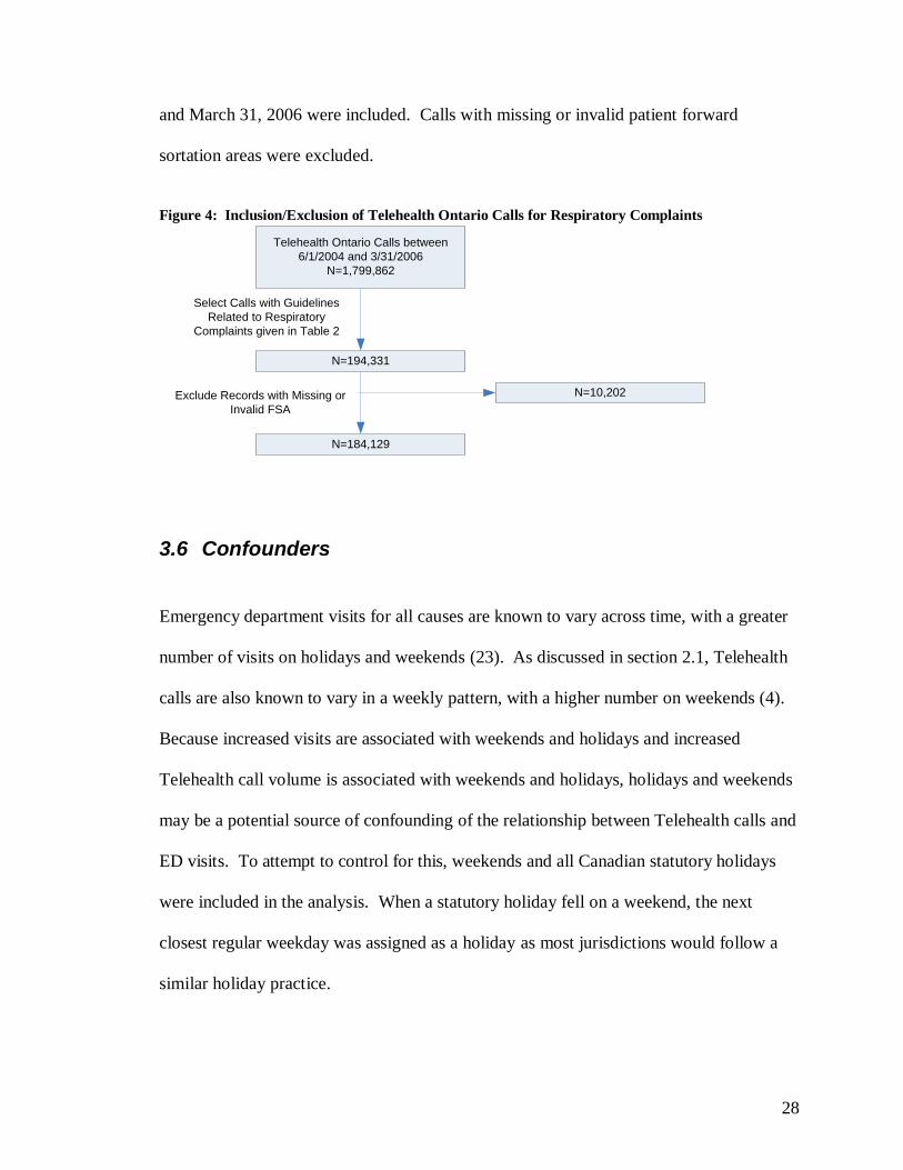
28
and March 31, 2006 were included. Calls with missing or invalid patient forward
sortation areas were excluded.
Figure 4: Inclusion/Exclusion of Telehealth Ontario Calls for Respiratory Complaints
Telehealth Ontario Calls between
6/1/2004 and 3/31/2006
N=1,799,862
N=194,331
Select Calls with Guidelines
Related to Respiratory
Complaints given in Table 2
N=184,129
Exclude Records with Missing or
Invalid FSA
N=10,202
3.6 Confounders
Emergency department visits for all causes are known to vary across time, with a greater
number of visits on holidays and weekends (23). As discussed in section 2.1, Telehealth
calls are also known to vary in a weekly pattern, with a higher number on weekends (4).
Because increased visits are associated with weekends and holidays and increased
Telehealth call volume is associated with weekends and holidays, holidays and weekends
may be a potential source of confounding of the relationship between Telehealth calls and
ED visits. To attempt to control for this, weekends and all Canadian statutory holidays
were included in the analysis. When a statutory holiday fell on a weekend, the next
closest regular weekday was assigned as a holiday as most jurisdictions would follow a
similar holiday practice.

29
3.7 Geographic Grouping of Telehealth Calls and Emergency Visits
The analysis performed in this study was carried out by geographical regions that
correspond approximately to each of the 36 public health unit regions in Ontario. Both
the NACRS and Telehealth Ontario data sets contain patient/caller postal code forward
sortation area (FSA) information, which is the first three digits of the individual’s postal
code (to protect the identities of individuals, complete postal code information was not
available).
An exact mapping between FSA and health unit is not possible as the region
corresponding to a single FSA may overlap with the regions corresponding to two or
more health units. To address this issue, a mapping between FSA and approximate public
health unit region was created as follows:
In Canada, census geography is broken down into census subdivisions, dissemination
areas, and blocks (from least to most granular) (51)(52). Statistics Canada provides a
correspondence file between dissemination areas and health region boundaries (53)(54)
and a postal code conversion file which includes all the dissemination areas for a given
FSA (51). A dissemination area only falls into one health region; however, each
dissemination area can be linked to more than one FSA. For each FSA in Ontario, the
associated dissemination areas in the postal code conversion file were used to match the
FSA to one or more health regions. The correspondence file also included the 2001
census population for the dissemination area. For a given FSA, the population was

30
summed for each unique health region sharing a geographic area with that FSA. The
public health unit with the largest census population was assigned to that FSA. In this
way, a one-to-one mapping between FSA and PHU was established. As the developed
FSA groupings do not represent exact PHU areas, the approximation should be
noted in all the results that follow.
Time series of calls and visits for respiratory complaints for each approximate PHU
region were obtained using this FSA mapping and the date information in the call and
visit data.
3.8 Analytic Techniques for Establishing the Relationship between Calls and Visits
3.8.1 Background
This thesis attempted to establish a useful relationship between the time series of
Telehealth Ontario calls for respiratory complaints and the time series of emergency
department visits time series for respiratory illness, for each health unit in Ontario.
Specifically, it was desired to know if the number of calls from the current day and those
from several days in the past were predictive of future emergency department visits. For
example, one may want to know how well the calls for the past 10 days predicted the
number of visits 3 days in advance. One could also ask the same question for 4, 5, 6 or
more days in advance. Therefore, this thesis examined multiple associations between
calls and visits, one association for each day in advance. This can be thought of an
analogous but different and more sophisticated approach to looking at the correlation

31
between time series at multiple lags as was done by van Dijk et al., discussed in section
2.1.
Characterization of this association can be thought of as a type of dynamic regression
problem (34). A mathematical model to quantify the relationship between a variable and
a set of predictor variables can be built from a first-principles understanding of the
relationship between variables, or by taking an empirical approach using measurement
data. In this latter approach, the model is sometimes referred to as a ―black-box‖ model
as we ignore how the physical process works (i.e. ignore the first principles approach) in
building the model and care only that the relationship between variables is accurately
described. In the engineering literature the term ―system identification‖ is used to refer to
the process of building a mathematical model describing the dynamic relationship
between two or more time series from observed data. The ―system‖ is a physical or
hypothetical process that transforms one or more input time series (independent variables)
into one or more output time series (dependent variables). System identification seeks to
build a mathematical description of how the system transforms its inputs into outputs.
There have been many methods developed to do this (55)(56). All three analytic time
series techniques applied in this thesis have been developed and used for the development
of black-box models of systems. A brief introduction to these methods is presented here.
Figure 5 illustrates the relationship between Telehealth Ontario calls and emergency
department visits framed as a system identification problem. This follows a standard
representation (57). The emergency department visit time series, y(n) (the system output
or dependent variable), is assumed to depend on past and present Telehealth Ontario calls,

32
u1(n), and holidays/weekends, u2(n) (the system inputs or independent variables). The
variable n indicates the time in days. All three of these time series are subject to
measurement error (for example miscoded reason for calls or visits). The error in calls is
represented by the noise series w1(n), w2(n) represents the error in holiday/weekends, and
vy(n) represents the error in emergency visits.
Figure 5: The Dynamic Relationship between Calls and Visits Time Series Framed as a System
Identification Problem
+ Unknown
Deterministic,
Time-Invariant
Relationship
Telehealth
Calls, u1(n)
Call Noise,
w1(n)
+
Process
Noise, wp(n)
+
Output
Measurement
Noise vy(n)
Emergency Visits,
y(n)
Measured
Emergency Visits,
ym(n)+Holidays,
u2(n)
Holiday
Noise, w2(n)
Shaping
Filter
The process noise, wp(n), and the associated shaping filter account for the fact that our
description of the relationship between time series may be imperfect because of missing
explanatory time series, a poorly chosen model structure, or a poor parameterization of
the chosen model structure (these are sometimes referred to as disturbances) (35,56).

33
Some model structures attempt to include a description of these disturbances effects.
Incorporation of these can improve results when the models are used to generate forecasts
(56). Other model structures do not include a description of the process noise: ignoring it
may have negligible impact on model performance if the inputs we have chosen to model,
u1(n) and u2(n), describe enough of the variation in the output (i.e. high signal-to-noise
ratio) (56).
3.8.2 Numerical Algorithms for Subspace State Space System Identification
ARMA (AutoRegressive Moving Average, univariate), ARX (AutoRegressive with
eXogenous input), and ARMAX (AutoRegressive Moving Average with eXogenous
input) time-series models are all variants of the ARIMA class of models. This class of
models has been investigated by previous studies as methods to create forecasts for health
services demand (Table 1). The ARIMA class of models have been shown to be special
cases of the state-space representation for a dynamic deterministic-stochastic process
(34,35,56,58). The state space representation uses a set of auxiliary variables, called state
variables, to describe the relationship between the predictor time series and the dependent
time series. The state variables allow the relationship to be expressed as a set of first-
order difference equations; the number of state variables in the model is referred to as the
order of the system (56).

34
The innovations form of the state-space representation is given by (56):
)()()()1( nKenBunAxnx
Equation 3-1
)()()()( nenDunCxny
Equation 3-2
where
x(n) is a vector of state variables
u(n) is a vector of system inputs
y(n) is a vector of system outputs
e(n) is the innovation vector
A, B, C, D, K are matrices of appropriate dimensions
Two general approaches for the identification of A, B, C, D, K using input-output data are
the Prediction Error Method (PEM) and Numerical Algorithms for Subspace State Space
System Identification (N4SID)(30,59). Briefly, N4SID methods construct an estimate of
a sequence of state vectors, x(n), of the state-space model given in Equation 3-1 and
Equation 3-2 from the observed input-output data. To do this, an approach similar to a
principal components analysis is taken (30). Once this state sequence is obtained, it is
possible to use regression to obtain a least-squares estimate of the system matrices C, D
and then A, B and K (56). The PEM method takes a fundamentally different approach
and suffers from a number of problems which are not encountered using the N4SID class
methods; therefore, the N4SID approach is preferable under many circumstances (59,60).

35
The N4SID algorithms have been implemented in the MATLAB System Identification
Toolbox (56). This software was used to fit linear state space models describing the
relationship between calls and visits. Further description of how this was done is given in
section 3.8.5.
Since the ARIMA, and in particular the ARMAX, model structures are a special case of
the state-space representation, the state space representation of the time series model was
included in the analysis to serve as a baseline with which to compare the novel non-linear
approaches. In this way, the advantage of accounting for possible non-linearity in the
calls to visits relationship could be assessed.
3.8.3 Fast Orthogonal Search
Fast Orthogonal Search (FOS) is a novel method for developing a non-linear difference
equation or other model of unknown structure (in contrast to the linear difference
equation described by the state-space method) of a dynamic system proposed by
Korenberg (61). The nonlinear difference equation model describes the relationship
between the current number of emergency department visits, y[n], current and past
number of Telehealth Ontario calls, u1[n], u1[n-1], u1[n-2], etc…, and current and past
values of an indicator variable for holidays/weekends, u2[n], u2[n-1], u2[n-2], etc… , and
past values of the number of emergency visits, y[n-1], y[n-2], etc… and is of the form:

36
M
m
mm nenpany0
][][][
Equation 3-3
where
n is the time index, n=0, 1, 2, …
p0=1
][]...[][]...[][]...[][210 2121111 jjjm qnuqnulnulnumnymnynp is the
general form of each term in the difference equation for m>0
am is a scalar coefficient
e[n] represents the error
and
j0 is the number of y factors, j0≥0
j1 is the number of u1 factors j1≥0
j2 is the number of u2 factors j2≥0
mk is the lag in kth
y factor, mk≥1
lk is the lag in the kth u1 factor, lk≥0
qk is the lag in the kth u2 factor, qk≥0
FOS searches a set of possible candidate terms, {cm[n]}, for the most significant terms
that minimize the mean square error over a training data set. Each of the candidate terms
in the set {cm[n]} has the general form shown above for pm.

37
Briefly, the method works by adding terms to the difference equation model from a set of
candidate terms, {cm[n]}, one at a time. Terms are selected based on a measure of the
reduction in the mean square error (MSE) of the model fit over the training data after
having added that particular term to the model. The candidate offering the largest
reduction in MSE is chosen and the process is repeated until the MSE has been reduced to
a predetermined level or a certain number of terms have been accepted into the model.
The reduction in MSE by adding a given candidate term to the model can be simply stated
in terms of a set of orthogonal basis functions {wm[n]} spanning the set {pm[n]} of all
terms in the model plus the candidate under consideration. One key to FOS is how the
measure of the reduction in MSE is calculated for each candidate term. Because the
number of potential candidate terms can be extremely large, calculating the MSE
reduction for each term could take a great deal of time as finding {wm[n]} is
computationally intensive. With the FOS algorithm, the set {wm[n]} are never actually
calculated, yet a measure of the reduction in MSE is still obtained, leading to faster
identification of the candidate which reduces the MSE by the largest amount (hence the
―Fast‖ in Fast Orthogonal Search) (62). To choose M terms for the model out of C
candidates using N values of time, FOS requires on the order of MNC multiplications.
FOS is related to an algorithm by Desrochers (63) for approximating static nonlinear
models where, amongst various differences, the computational and memory requirements
are proportional to the square of the number of candidates, whereas in FOS they depend
linearly on the number.

38
3.8.4 Parallel Cascade Identification
Parallel Cascade Identification (PCI) is a novel method for developing a model of a non-
linear time-invariant system and has been applied successfully in a wide-range of system
identification problems (64-70).
Consider a discrete-time (i.e. data are sampled at evenly spaced instants in time), time-
invariant (i.e. the relationship between time series does not change over time), causal (i.e.
output only depends on present and past values of the input(s)), finite-memory system
(i.e. output only depends on inputs up to a finite time in the past). Suppose that its output
is a continuous mapping of its input, in that ―small‖ changes in the input result in ―small‖
changes in the output. Then it follows from the Stone-Weierstrass theorem that such a
system can, over a uniformly bounded set of input signals, be approximated to an
arbitrary degree of accuracy by a discrete-time, finite-memory Volterra series of
sufficient, but finite, order. Korenberg further showed that any discrete-time, finite-
memory, finite-order Volterra series can be represented with an arbitrary degree of
accuracy by a parallel array of ―LN cascades‖. Each ―LN cascade‖ is a system consisting
of a dynamic linear element (L), described by a finite duration impulse response,
followed by a static non-linearity (N). PCI is a method of identifying these cascades using
observed input-output data from the system(64). To summarize, PCI has been
theoretically proven capable of modeling a class of non-linear time series associations
(more specifically any system having a Wiener series expansion).

39
A simplistic explanation of how PCI works for a single-input single-output system is as
follows (64,69,70):
In this explanation we note a discrepancy between the language used in signal processing
and that used in biostatistics. In this section ―cross-correlation‖ refers actually to the
cross-covariance familiar to statisticians and biostatisticians. Starting with the first
cascade, identify the impulse response of the dynamic linear element (L) in the cascade
using the first-order cross-correlation of the system input with the system output or a slice
of a second- or higher-order cross-correlation, determined at random, of the system input
with the system output. In the case of the latter, addition or subtraction (also determined
at random) of weighted delta functions is required for diagonal elements of the cross-
correlations, in order to ensure convergence. Calculate the output of the linear element
and fit a polynomial that minimizes the mean square error of the residual, where the
residual for the first cascade is the difference between the polynomial’s output and the
output of the system to be identified. Determine the reduction in mean-square error in the
residual as a result of adding this cascade (which is equal to the mean-square of the
cascade output); reject the cascade if this reduction is not above a certain threshold (to
avoid fitting noise). Subsequent cascades are added in a similar fashion using the residual
between the system output and the output of the model consisting of all the cascades
identified to date.
The above algorithm is easily modified to accommodate multiple inputs, as is done in this
thesis, by randomly selecting one of the inputs or cross-products of the inputs when
computing the first- or higher-order cross-correlation (64,70).

40
There are no special requirements for the input-output data required to fit (train) a PCI
model as there is with some other methods of non-linear system identification. The only
requirement is that the training data should be sufficiently ―rich‖. Practically, ―rich‖
means that it should cover the range of inputs and outputs expected when the model is
applied (69,70). Since respiratory illness shows a yearly pattern that peaks during
influenza season (46), in terms of the current study, this means that the training set cover
at least one year of data. For this reason approximately half of the two years of study data
was used to train the models and the other half was used to validate (assess the fit) of the
models.
3.8.5 Model Implementation
There were two inputs (independent variables) to the models created: 1) an indicator
variable coded 1 for weekends/statutory holidays and 0 otherwise, u2, and 2) the number
of Telehealth Ontario calls, u1, for each 24 hour period. There was one output (dependent
variable): the number of emergency department visits, y, for each 24 hour period.
Process noise is ignored when constructing a state space model for the system for two
reasons. First, we do not have access to the error for past predictions due to the fact that
NACRS visit data is not available until the end of the fiscal year (44,45), therefore we
cannot use the sequence of past errors to improve future forecasts. Second, the Parallel
Cascade Identification and Fast Orthogonal Search algorithms are not implemented to

41
include these effects, although it is possible to do so, and so to make them comparable
with the Subspace Identification Algorithm, the latter ignores fitting a disturbance model.
Forecasting models were constructed for each of the days ahead to be predicted. This
included a zero-day-ahead forecaster that produced a forecast of the number of visits for
the current day (i.e. at the end of that day, assuming all calls for that day had been
received). A total of 15 models were created to produce such forecasts up to 14 days in
advance. Note that a 14-day-ahead predictor could have been used to produce an estimate
for all of these cases (i.e. 0, 1, 2, 3, 4, …, 14 days in advance), but as will be shown later,
in general, a n-day-ahead predictor was more accurate than an n+k-day-ahead predictor,
where k>0.
To fit (train) a model using the Parallel Cascade Identification (PCI), Fast Orthogonal
Search (FOS), or N4SID (SS) algorithms to create an k-day ahead predictor, visits were
advanced in time (i.e. left-shifted) by k-days relative to the calls. The weekend/holiday
indicator variable input was also advanced in time by the same k-days. This is reasonable
to do as upcoming weekends/holidays are known in advance. Specifically, a k-day ahead
predictor described the mathematical relationship between the following input and output
time series:

42
Input (predictor) time series:
Telehealth Ontario calls time series: u1(n)
Holiday/weekend indicator variable time series: u2(n+k)
Output (dependent) time series:
Emergency department visits time series: y(n+k)
where n=0, 1, … could take on any time index over the training data.
When generating the forecasted values in this thesis, it was NOT assumed that the actual
past emergency department visits are available to the forecasting model. This is realistic
if the algorithms were to be applied in a real-time, prospective manner as hospitals in
Ontario are only required to submit the information used to generate the NACRS database
to CIHI at the end of the fiscal year (44,45). The specific implications of this are as
follows:
1) When making forecasts in the case of Fast Orthogonal Search, it may be necessary to
use past values of the system output (emergency department visits) to make future
forecasts of visits; this can be seen from Equation 3-3 which includes the possibility
of past values of the output in the difference equation. In this case, the forecasted values
of the past output, rather than the actual values of that output were used.
2) The state space model in Equation 3-1 allows for a disturbance model by specifying
the K matrix which uses values of the error to compute the next state vector. Since the
error is not available to the model, the term containing K in Equation 3-1 is ignored.

43
All models were programmed in the MATLAB software package (71). The state-space
model was identified using the Numerical Methods for Subspace State Space System
Identification (N4SID) algorithm implemented in the MATLAB system identification
toolbox (71). The Parallel Cascade Identification algorithm and Fast Orthogonal Search
algorithm were implemented by the author. Both implementations were validated using
test data generated from a known non-linear difference equation prior to using them to
build models in this thesis.
A trial-and-error process was used to determine appropriate model structure for the three
types of models. Specifically, this included defining structural choices given in Table 6.
Table 6: Structure Choices Required for each Type of Prediction Model
Model Type Structure Choices
State Space Number of state variables (system order)
Difference Equation Determined by Fast
Orthogonal Search
Total number of terms in the difference equation
Maximum number of u1, u2, and y factors in each term
in the difference equation
Maximum lag for each u1, u2, and y factor
Parallel Cascade Number of cascades
Memory length of the linear elements
Order of the static nonlinearity in each cascade

44
3.8.5.1 State Space Model using Subspace Identification
A state-space model with 10 state variables was used for all health units. Preliminary
investigation indicated that models of order 8 or 9 allowed good fits to be achieved for
most health units when the algorithm was allowed to choose automatically. This
dimension of the state space model was chosen to ensure rough comparability with other
techniques: the number of state variables (also referred to as the system order) is related
to the number of lags in the difference equation representation of a state space model
(56). The Parallel Cascade model allowed lags from 0 to 9 in the inputs (i.e. the linear
element in each cascade had a memory length of 10) and the difference equation
generated by FOS allowed for lags up to 10 in any factor in any term (refer to
implementation details of FOS and PCI implementations below). The N4SID algorithm
properties were set to optimize for prediction and stability (56); without specifying these
options, many of the models found were unstable (i.e. resulted in extremely large/small
forecasts and/or large oscillations in the forecasts).
3.8.5.2 Parallel Cascade Model Using Parallel Cascade Identification
The Parallel Cascade Identification algorithm was implemented as described by
Korenberg (64). This section describes the model structure chosen and modifications to
the algorithm.
The Parallel Cascade models incorporated a maximum of three cascades (it was observed
that the mean square error did not decline much after three cascades had been added to

45
the model over the training data). The linear element in each cascade had a memory
length of 10 samples (i.e. calls from 0 to 9 days in the past were used by the model). A
maximum second-order cross-correlation was used in identifying the impulse response of
the linear element. The static non-linearity was limited to only a second-order
polynomial. Limiting the order of the polynomial prevented over-fitting (loss of
generalizability of the model) on the training data which could result in large deviations
in the forecasts over the validation data.
An adaptive approach was taken to the cutoff value used in determining whether a given
cascade was accepted in the model in an effort to only accept the best cascades into the
model. Specifically, the suggested cutoff given by Korenberg (64):

46
)(1
4)( 22
1 nyRT
nz ii
Equation 3-4
where:
zi+1(n) is the output of the i+1 cascade to be added
yi(n) is the residual after adding the ith cascade to the model
T is the length of the training time series
R is the maximum lag used by the linear element
the over-bar represents the time average from n = R to n = T
was modified to:
)(1
)( 22
1 nyRT
nz ii
Equation 3-5
where λ was adjusted from an initial value of 40, and then decreased in an exponential
fashion (by dividing by a factor of 1.5) each time more than 100 cascades were rejected.
3.8.5.3 Difference Equation Model Using Fast Orthogonal Search
The Fast Orthogonal Search algorithm was implemented as described by Korenberg (61).
Ten terms were allowed in the difference equation model generated by the Fast
Orthogonal Search algorithm. Each term, other than the constant term, contained factors
with lags of up to 10 days.

47
Trial and error indicated that the model generalized better when a number of linear terms
were allowed in the model first before adding terms containing cross-products. Linear
terms are terms which have only one factor; in terms of pm in Equation 3-3 this means
only one of j0, j1, j2 is non-zero. Therefore the model included a constant term, seven
linear terms, and two cross-product terms. The two non-linear or cross-product terms had
up to one factor in the call input, one factor related to the holiday input, and at most one
output factor. This approach to forcing certain terms into the model before others was
similar to that used by Minz and Korenberg (72), but did not involve pre-screening of the
terms. Cross-product terms were not limited to cross-products of the linear terms
previously accepted into the model.
3.9 Measures
For each health unit, the time series was divided into a training dataset (45% of the data
or 301 days) and a validation dataset (55% of the data or 368 days). Refer to section
3.8.4 for justification of this split in the data. The training dataset was used to fit the
models. Each model was assessed using the measures described below over the
validation dataset. Models producing forecasts of the number of daily visits up to 14 days
in advance were created. A maximum 14-day lead was chosen because previous work
indicated a significant correlation in the calls/visits time series of up to 15 days in
advance (1). A period of time equal to the maximum lag used in the models (10 days)

48
was excluded at the beginning of the validation datasets to allow the models to settle
before performance was assessed.
3.9.1.1 Qualitative Assessment of Model Fit
Model fit was assessed qualitatively by visually comparing plots of the forecasted time
series of hospital emergency visits and the actual time series of visits. Plots can provide
more information than statistical summary measures of error. For example, summary
measures such as average error can fail to capture short-term but important deviations of
the predictions from the actual time series, and also fail to adequately characterize the
temporal variation in the error. Plots of the error between the predicted and actual
number of visits were also generated.
Plots for both the daily number of visits and weekly aggregate number of visits were
generated. Plots for daily number of visits can be generated for any one of the k-day
ahead predictors. Plots of the weekly aggregate number of visits can be generated for one
week ahead (the next 1 to 7 days) or two weeks ahead (the next 8-14 days). The one
week ahead aggregate number of visits is generated by summing the 1-day, 2-day, 3-day,
4-day, 5-day, 6-day, and 7-day ahead (lead) predictions. A concrete example of this is
illustrated in Figure 6 assuming it is Monday and all calls have been received for the day
(note that the start of the week was arbitrary and the choice of Tuesday is only for
illustrative purposes). The two week ahead aggregate number of visits is generated in a
similar manner by summing 8-day through 14-day ahead predictions. Plots of the weekly

49
aggregate number of visits remove the cyclical weekly pattern of visits which can act to
visually obscure trends. Aggregation keeps the plots more interpretable than if filtering
methods such as a moving average were applied. Because they remove the cyclical
weekly pattern, this approach controls for the possible confounding effect of weekends,
allowing the ability of Telehealth calls to predict emergency department visits to be
assessed (rather than assessing the ability of Telehealth AND weekends/holidays to
predict visits). Note that there will still be some residual confounding as aggregating on a
weekly basis does not control for the effect of holidays.
Figure 6: Prediction of Aggregate Hospital Visits over a period of 1-7 Days in the Future (1 Window
Ahead) and a period of 8-14 Days in the Future (2 Windows Ahead)
Su Mo Tu We Th Fr Sa Su Mo Tu We Th Fr Sa Su Mo Tu
1 Week Ahead 2 Week Ahead
Current Date
1-D
ay L
ea
d
Pre
dic
tor
2-D
ay L
ea
d
Pre
dic
tor
3-D
ay L
ea
d
Pre
dic
tor
4-D
ay L
ea
d
Pre
dic
tor
5-D
ay L
ea
d
Pre
dic
tor
6-D
ay L
ea
d
Pre
dic
tor
7-D
ay L
ea
d
Pre
dic
tor
8-D
ay L
ea
d
Pre
dic
tor
9-D
ay L
ea
d
Pre
dic
tor
10
-Da
y L
ea
d
Pre
dic
tor
11
-Da
y L
ea
d
Pre
dic
tor
12
-Da
y L
ea
d
Pre
dic
tor
13
-Da
y L
ea
d
Pre
dic
tor
14
-Da
y L
ea
d
Pre
dic
tor
Predictors
Used:
3.9.1.2 Quantitative Assessment of Model Fit
Quantitative assessment of the fit of the model over the validation set was made by
capturing the median, 25th percentile, and 75
th percentile of the error in the daily and
weekly aggregate number of emergency department visits for each of the prediction
methods over the validation data.
Two summary measures of the error were used. The percent mean square error (%MSE)
is defined as (73):

50
%100))()((
))()((%100
))()((
))()((%
22
2
2
2
nyny
nzny
nyny
nznyMSE
Equation 3-6
The percent mean absolute prediction (percentage) error (MAPE) is defined as (34):
%100)(
)()(
ny
nznyMAPE
Equation 3-7
where
the over-bar represents the time average
y(n) is the value of the actual time series at time n
z(n) is the value of the forecast (predicted) time series at time n
Justification for the choice of these measures follows.
The MAPE has been used as a standard measure of forecasting accuracy (34) and is an
intuitive measure of the size of the forecasting errors. It allows the results of this study to
be compared with past studies that have used this measure. However, it has two
drawbacks. First, Equation 3-7 is not defined when the actual number of visits is zero.
Zero visits occurred in some of the smaller health units: Perth District Health Unit,
Timiskaming Health Unit, Brant County Health Unit, and Elgin-St. Thomas Health Unit.
This measure cannot be used in these health units. A second drawback is that forecasting
errors of equal magnitude above and below the actual value give different percentage
errors, with over-predictions being penalized more than under-prediction. For example if

51
the actual value is 130 and the forecast value is 100 (a difference of 30—under-
prediction), the MAPE is 23%, but when the actual value is 100 and the forecast is 130
(also a difference of 30—over-prediction), the MAPE is 30% (74,75). Although
corrections for this have been proposed, there are still issues (76). For this reason the
comparison between forecasting methods was performed using %MSE, and MAPE is
presented as an alternative mainly for comparison with past and future studies.
%MSE is an alternative measurement of accuracy without this problem, but with the
drawback that it is less intuitive. %MSE is a relative measure of the variation in the
prediction error (sum of squares of the error) compared to the variance in the time series
we are trying to predict. A model that fits well will have an error variance much lower
than the variance in the actual time series to be predicted.
3.9.1.3 Ability to Predict Increases
While plots of the actual and forecasted time series, the error time series, summary error
statistics, and summary measures of fit (%MSE and MAPE) discussed in the previous
sections provide a way to compare models, using any of these to interpret the usefulness
of the models can still be difficult. A model might appear to fit well according to these
measures, but be of little practical value.

52
Usefulness of the predictions was assessed in terms of the ability to predict future
increases in emergency department visits. Since it is desirable to be able to forecast
hospital bed shortages or the presence of a disease outbreak, the ability to warn of
increases in the aggregate number of future visits over a given window of time is
important. Aggregation of visits over a window of several days was necessary because
the day-to-day volatility in the number of visits was high and it was desirable to capture
increases in longer term trend rather than in daily volatility.
3.9.1.3.1 Windowing Method
Visits were aggregated over four- or seven-day windows that did not overlap. Analyses
were carried out over the validation dataset. A window size of seven-days eliminates the
cyclical weekly pattern in visits and calls on weekends thereby providing control for the
confounding effect of weekends (as discussed in section 3.9.1.1). The four-day window
was chosen to assess the combined predictive ability of calls and holidays/weekends over
a shorter time frame as a comparison.
The ability to predict an increase in the aggregate number of visits over a seven-day
window (i.e. weekly aggregate) either 1-7 days in the future (referred to as a one-window-
ahead/one-week-ahead forecast), or 8-14 days in the future (referred to as a two-
windows-ahead/two-week-ahead forecast) was assessed. Increases were relative to a
baseline seven-day window, consisting of the immediately preceding seven-day period.
The aggregate number of visits predicted for one-window-ahead (1-7 days in the future)

53
consists of the sum of the forecasted visits using the 1-day, 2-day, 3-day, 4-day, 5-day, 6-
day and 7-day lead predictors. Note that it is possible to use only a seven-day ahead
predictor to generate forecasts for the 1-window-ahead aggregate forecast; however, as
will be shown later, the %MSE generally increases as the prediction lead increases,
meaning that the forecasted visits generated by the n-day ahead predictor more accurately
reflect the true visits than those generated by the n+k-day, where k>0, ahead predictor.
Therefore, we should use the predictor with the smallest lead possible if we wish to
generate the most accurate forecasts. Forecasts for the two-windows-ahead were
generated in a similar manner.
The aggregate number of visits over the baseline window was calculated using forecasted
visits because data from the NACRS database are not available immediately; hospitals are
only required to submit their data to CIHI for inclusion in the NACRS database by the
end of July for the preceding fiscal year (44). Although it might seem intuitive to use the
zero-lead predictor to do this because it is more accurate that an k-lead predictor, where
k>0, as will be shown later, in practice this can give poor results because the predicted
time series generated by the zero-lead predictors can be quite different from the 1-7 or 8-
14 day predictors (for example one sequence can be slightly offset from the other). For
this reason, the corresponding past 1-7 or 8-14 day predictors were used in creating the
baseline visits.
An analogous approach was taken for the four-day window, the only difference being that
visits were aggregated over four days instead of seven.

54
3.9.1.3.2 Method used to Flag Increases
Increases in the aggregate number of visits for the nth
-window-ahead over the baseline
window was calculated as follows:
100%
B
BWn
A
AAI
Equation 3-8
where
%I is the percentage increase for the nth
-window-ahead over baseline
AWn is the aggregate number of forecasted visits over the nth-window-ahead
AB is the aggregate number of predicted visits over the baseline window.
To clarify this scheme, consider Figure 7. Suppose it is currently Tuesday (not yet the
end of the day) and it is desired to predict whether there will be an important increase in
the number of visits over the following seven-day window (1 window ahead, or Tuesday
(today) through Monday, inclusive) relative to the baseline aggregate number of visits
over the previous seven-day window (baseline window). Predictions from the 1-day lead
predictor through to the 7-day lead predictor are summed to give AW1 (AWn with n=1) in
Equation 3-8. This sum from the previous period (i.e. that generated last Tuesday) is used
for AB in Equation 3-8. The percentage increase over baseline is calculated using
Equation 3-8 and compared to a threshold (this threshold is discussed below). If the
percentage increase is above the threshold, the window is flagged. The actual visits time
series is flagged in a similar manner except that AWn and AB in Equation 3-8 are
calculated using actual visits rather than forecasted values.

55
Figure 7: Ability to Predict Important Increases in Visits over a Seven-Day Window
Su Mo Tu We Th Fr Sa Su Mo Tu We Th Fr Sa Su Mo Tu
1 Window Ahead 2 Windows Ahead
Current Date
1-D
ay L
ea
d
Pre
dic
tor
2-D
ay L
ea
d
Pre
dic
tor
3-D
ay L
ea
d
Pre
dic
tor
4-D
ay L
ea
d
Pre
dic
tor
5-D
ay L
ea
d
Pre
dic
tor
6-D
ay L
ea
d
Pre
dic
tor
7-D
ay L
ea
d
Pre
dic
tor
8-D
ay L
ea
d
Pre
dic
tor
9-D
ay L
ea
d
Pre
dic
tor
10
-Da
y L
ea
d
Pre
dic
tor
11
-Da
y L
ea
d
Pre
dic
tor
12
-Da
y L
ea
d
Pre
dic
tor
13
-Da
y L
ea
d
Pre
dic
tor
14
-Da
y L
ea
d
Pre
dic
tor
Predictors
Used:
Su Mo Tu We Th Fr Sa
Baseline Window
Estimate of Baseline Visits using Previous 1
Window Ahead or 2 Window Ahead Forecasts
Two different types of thresholds were specified: 1) a fixed threshold at a zero percent
increase, and 2) a threshold whose percentage increase cutoff depended on the number of
visits.
The purpose of using a fixed threshold at zero was to test whether or not the forecasts
could accurately predict the sequence of increases and decreases in actual visits.
As discussed above, for planning purposes it might be desirable to warn of a large
upcoming increase in the number of emergency visits rather than simply an increase. A
large change in the number of visits may also indicate disease outbreak. The threshold
defining a ―large percentage increase‖ was variable depending on the actual number of
visits over the baseline window. A variable threshold was necessary because for a small
number of visits, a few additional visits can represent a large percentage increase, but this
increase is not important. For example, if the baseline window had 10 visits and the
window ahead being considered had 12 visits this would be a 20% increase. If the
baseline window for the same health unit now had 100 visits and the window ahead being
considered had 120 visits, this also represents a 20% increase. While the former case is
probably not an important increase, the latter might be.

56
The threshold used for flagging an increase, T, as a function of vbaseline (expressed as a
percentage) was defined as follows:
imum
ref
baseline
alnoimumimumbaseline Tv
vTTTvT minminmaxmax ,)(max)(
Equation 3-9
where
otherwiseb
baifaba
,
,,max
vbaseline is the number of visits over the baseline window
Tnominal is a nominal threshold
vref is a reference number of baseline visits where the threshold is the nominal
threshold and was set to the average number of daily visits over the training data
times the window size (for example to give the average number of weekly visits in
the case of a seven-day window),
Tmaximum is the threshold if there were zero visits
Tmininum is the minimum threshold, regardless of the number of visits
Figure 8 illustrates this variable threshold as a function of the baseline number of visits.

57
Figure 8: Threshold used for Flagging an Important Increases in the Number of Emergency
Department Visits
T
vref
Tmaximum
Tminimum
Tnominal
vbaseline
For the window of 1-7 days in advance, Tnominal was set to 10, Tminimum was set to 10, and
Tmaximum was set to 30. For the window of 8-14 days in advance, the thresholds were set
higher (as we are trying to detect ―important‖ increases after a longer period of time—
with more time, we expect higher variation). In this case Tnominal was set to 15, vref was
again set to the average number of daily visits over the training data times the window
size (to give the average number of weekly visits in the case of a 7-day window size),
Tminimum was set to 10, and Tmaximum was set to 60.
For example, using the values for 1-7 days in advance, with an average weekly number of
visits of 100, the nominal threshold with 100 visits in the baseline window is a 10%
increase; with 50 visits in the baseline window, the threshold is a 20% increase; with 20
visits in the baseline window, the threshold is a 26% increase.
This procedure for flagging increases was repeated using the time series for the actual
visits employing the same threshold and window definition—the only difference was that
the actual values for the number of emergency visits was used in the calculations
described above instead of those generated by k-day-ahead predictors.
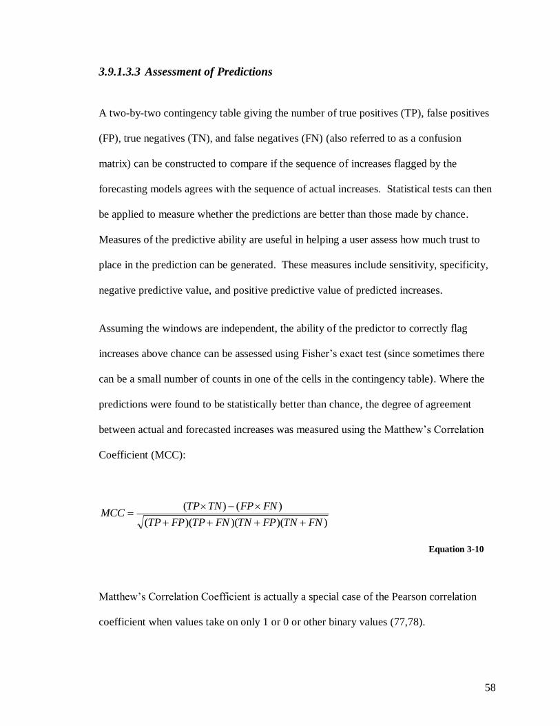
58
3.9.1.3.3 Assessment of Predictions
A two-by-two contingency table giving the number of true positives (TP), false positives
(FP), true negatives (TN), and false negatives (FN) (also referred to as a confusion
matrix) can be constructed to compare if the sequence of increases flagged by the
forecasting models agrees with the sequence of actual increases. Statistical tests can then
be applied to measure whether the predictions are better than those made by chance.
Measures of the predictive ability are useful in helping a user assess how much trust to
place in the prediction can be generated. These measures include sensitivity, specificity,
negative predictive value, and positive predictive value of predicted increases.
Assuming the windows are independent, the ability of the predictor to correctly flag
increases above chance can be assessed using Fisher’s exact test (since sometimes there
can be a small number of counts in one of the cells in the contingency table). Where the
predictions were found to be statistically better than chance, the degree of agreement
between actual and forecasted increases was measured using the Matthew’s Correlation
Coefficient (MCC):
))()()((
)()(
FNTNFPTNFNTPFPTP
FNFPTNTPMCC
Equation 3-10
Matthew’s Correlation Coefficient is actually a special case of the Pearson correlation
coefficient when values take on only 1 or 0 or other binary values (77,78).
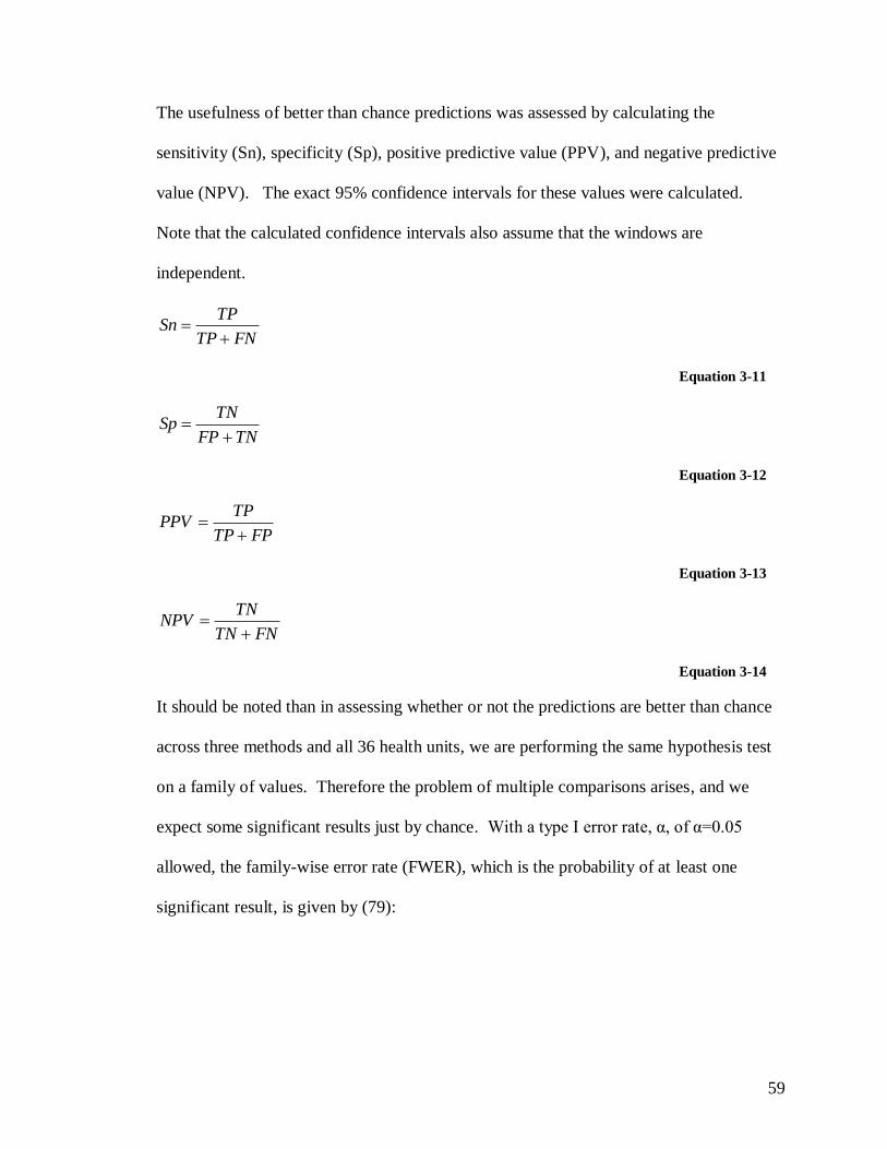
59
The usefulness of better than chance predictions was assessed by calculating the
sensitivity (Sn), specificity (Sp), positive predictive value (PPV), and negative predictive
value (NPV). The exact 95% confidence intervals for these values were calculated.
Note that the calculated confidence intervals also assume that the windows are
independent.
FNTP
TPSn
Equation 3-11
TNFP
TNSp
Equation 3-12
FPTP
TPPPV
Equation 3-13
FNTN
TNNPV
Equation 3-14
It should be noted than in assessing whether or not the predictions are better than chance
across three methods and all 36 health units, we are performing the same hypothesis test
on a family of values. Therefore the problem of multiple comparisons arises, and we
expect some significant results just by chance. With a type I error rate, α, of α=0.05
allowed, the family-wise error rate (FWER), which is the probability of at least one
significant result, is given by (79):

60
kFWER )1(1
Equation 3-15
where
k is the number of independent hypothesis tests performed
α is the probability of a type I error in the predictions over the validation set for
any single combination of health unit, method, and windows ahead
Conservative adjustment of the p-values for multiple comparisons can be made by the
Bonferroni method, which involves multiplication of the Fisher’s exact test p-values by
the number of experiments, k.
kppadj
Equation 3-16
Note that the Bonferroni correction is a very conservative adjustment (79).
3.9.1.3.4 Comparison to Using Telehealth Alone
It has been shown that Telehealth calls appear to precede visits at the provincial level (1).
Therefore, Telehealth calls time series alone may predict future increases in visits. A
comparison between the method of flagging increases discussed above and a simple
method using Telehealth calls alone should be made to ensure that the models used to
generate the forecasts provide value. In other words, is it really necessary to go to all of
the trouble to use forecasted values produced by the models to predict increases or could
a simple predictor be built using only the raw Telehealth calls time series?

61
To answer this question, Telehealth calls were aggregated over a given window and again
over the window prior to that. The percentage change in calls over these two windows
was calculated using Equation 3-8 (with AWn representing calls for the given window,
and AB calls from the previous window) and this percentage increase was considered to
be a ―test value‖. Because Telehealth calls appear to represent a scaled version of the
number of visits for many health units (refer to Figure 9 for example), the same threshold
used for actual increases (described above) was not employed for flagging increases using
the ―test value‖. Instead, it was desired to know if using a threshold at any level yielded a
useful predictor. Answering this question can be accomplished by calculating the area
under the receiver operating characteristic (ROC) and associated confidence limits
(78,80,81). In other words, the problem is viewed as that of determining the usefulness of
a diagnostic variable as is done in clinical epidemiology.
As just noted, in addition to a point estimate, confidence limits can be generated for the
area under the receiver operating characteristic (AUROC) (80,81). In this analysis, the
confidence limits of the AUROC were not adjusted for possible correlation between
windows, nor were they adjusted to account for multiple comparisons.

62
Chapter 4 Results
Although analyses were carried out for each of the 36 Health Units in Ontario, it would
be overwhelming to present detailed results such as plots for each health unit. Therefore
in sections where it is not feasible to include results for all health units, the City of
Toronto Health Unit and the Grey Bruce Health Unit are chosen as representative
examples. Justification for the choice of these two health units is as follows. According
to total and daily median number of emergency department visits, these two Health Units
are most important. These two health regions also provide contrast: the City of Toronto
Health Unit is an urban area with a relatively high ratio of daily Telehealth calls to daily
visits while the Grey Bruce Health Unit is a rural area with a relatively low ratio of daily
calls to daily visits.
4.1 Summary Statistics of Telehealth Ontario Calls and Emergency Department Visits by Health Unit
Table 7, Table 8, and Table 9 present summary statistics for the number of Telehealth
Ontario calls and emergency department visits for respiratory complaints for each
approximate health unit area in Ontario over the study period.
Table 7 gives the total number of hospital emergency department visits and Telehealth
Ontario calls over the study period for each health unit. Health units were ranked in
importance based on the overall number of emergency visits. Table 7 and all subsequent
tables are sorted according to this ranking. Note that ranking Health Units by the overall

63
number of ED visits is similar (with some exceptions) to ranking them by median number
of daily visits as can be seen by examining Table 8.
Table 8 presents summary statistics (25th percentile, median, 75
th percentile) of the daily
number of Telehealth Ontario calls and emergency department visits for respiratory
complaints over the study period. Health units with a higher median number of visits do
not necessarily also have a higher median number of calls. To highlight this, Table 9
presents the ratio of the median number of daily calls to the median number of daily ED
visits.
Table 10 presents basic descriptive statistics of the age of the individuals Telehealth calls
for respiratory complaints were about and of the age of patients visiting the emergency
department for respiratory illness.

64
Table 7: Total Telehealth Ontario Calls and Emergency Department Visits for Respiratory
Complaints by Health Unit over Study Period
Hospital Emergency
Department Visits
Telehealth Ontario Calls
Public Health Unit Name (Approximate1)
2001
Census
Population2
Total
Number
of Visits
Percentage
of Total
Total
Number
of Calls
Percentage
of Total
City of Toronto Health Unit 2,481,494 59,048 10.6 35,808 19.4
Grey Bruce Health Unit 152,965 32,018 5.8 2,457 1.3
Simcoe Muskoka District Health Unit 430,156 29,647 5.3 8,361 4.5
Niagara Regional Area Health Unit 410,574 25,261 4.6 5,405 2.9
Peel Regional Health Unit 988,948 25,111 4.5 17,032 9.3
City of Ottawa Health Unit 791,477 24,502 4.4 14,727 8.0
City of Hamilton Health Unit 490,268 23,280 4.2 6,261 3.4
York Regional Health Unit 729,254 18,633 3.4 14,069 7.6
Leeds, Grenville and Lanark District Health Unit 159,101 17,989 3.2 2,345 1.3
Middlesex-London Health Unit 403,185 17,862 3.2 6,166 3.3
Durham Regional Health Unit 506,901 17,647 3.2 8,732 4.7
The Eastern Ontario Health Unit 185,968 16,230 2.9 2,698 1.5
Peterborough County-City Health Unit 125,856 15,105 2.7 2,884 1.6
Hastings and Prince Edward Counties Health Unit 150,816 14,703 2.6 3,036 1.6
Waterloo Health Unit 438,515 14,413 2.6 8,853 4.8
The District of Algoma Health Unit 117,185 14,192 2.6 1,758 1.0
Renfrew County and District Health Unit 96,467 13,306 2.4 1,621 0.9
Thunder Bay District Health Unit 155,462 12,812 2.3 3,120 1.7
Porcupine Health Unit 88,205 12,558 2.3 1,696 0.9
Haliburton, Kawartha, Pine Ridge District Health
Unit
161,761 12,295 2.2 1,827 1.0
North Bay Parry Sound District Health Unit 120,353 12,230 2.2 2,663 1.4
Oxford County Health Unit 99,270 11,725 2.1 1,606 0.9
Lambton Health Unit 126,971 11,549 2.1 1,336 0.7
Chatham-Kent Health Unit 107,709 11,451 2.1 1,557 0.8
Haldimand-Norfolk Health Unit 104,575 11,297 2.0 1,431 0.8
Halton Regional Health Unit 375,229 11,210 2.0 7,451 4.0
Windsor-Essex County Health Unit 374,975 9,991 1.8 3,965 2.2
Northwestern Health Unit 77,823 9,906 1.8 1,673 0.9
Kingston, Frontenac, Lennox, Addington Health Unit 235,664 9,806 1.8 2,820 1.5
Sudbury and District Health Unit 190,474 8,183 1.5 2,723 1.5
Huron County Health Unit 59,701 6,857 1.2 798 0.4
Wellington-Dufferin-Guelph Health Unit 238,326 6,835 1.2 3,132 1.7
Perth District Health Unit 73,675 5,131 0.9 1,172 0.6
Brant County Health Unit 118,580 4,814 0.9 1,706 0.9
Timiskaming Health Unit 35,245 4,072 0.7 498 0.3
Elgin-St. Thomas Health Unit 81,553 3,458 0.6 742 0.4
Total 555,127 184,129
1 Refer to section 3.7
2 Calculated using the 2001 census population of the dissemination areas making up the approximate health unit grouping

65
Table 8: Summary Statistics of Daily Telehealth Ontario Call and Emergency Department Visit
Activity for Respiratory Complaints by Health Unit over Study Period Public Health Unit Name Number of Daily Visits Number of Daily Calls
Median (25th Percentile,
75th Percentile)
Median (25th Percentile,
75th Percentile)
City of Toronto Health Unit 75 (60, 103) 48 (35, 65)
Grey Bruce Health Unit 44 (30, 58) 3 (2, 5)
Simcoe Muskoka District Health Unit 41 (31, 52) 11 (8, 16)
Niagara Regional Area Health Unit 33 (25, 44) 7 (5, 10)
Peel Regional Health Unit 33 (25, 45) 23 (16, 32)
City of Ottawa Health Unit 33 (25, 45) 21 (13, 28)
City of Hamilton Health Unit 30 (24, 40) 8 (5, 12)
York Regional Health Unit 25 (19, 33) 19 (13, 26)
Leeds Grenville and Lanark District Health Unit 25 (18, 34) 3 (2, 5)
Middlesex-London Health Unit 23 (16, 32) 8 (5, 12)
Durham Regional Health Unit 24 (17, 32) 12 (8, 17)
The Eastern Ontario Health Unit 23 (16, 29) 3 (2, 6)
Peterborough County-City Health Unit 20 (14, 27) 4 (2, 6)
Hastings and Prince Edward Counties Health Unit 20 (13, 27) 4 (2, 6)
Waterloo Health Unit 19 (14, 26) 11 (8, 16)
The District of Algoma Health Unit 19 (14, 26) 2 (1, 4)
Renfrew County and District Health Unit 18 (13, 25) 2 (1, 3)
Thunder Bay District Health Unit 17 (12, 23) 4 (2, 6)
Porcupine Health Unit 17 (12, 23) 2 (1, 4)
Haliburton Kawartha Pine Ridge District Health 17 (11, 23) 2 (1, 4)
North Bay Parry Sound District Health Unit 16 (12, 22) 3 (2, 5)
Oxford County Health Unit 15 (11, 22) 2 (1, 3)
Lambton Health Unit 15 (11, 21) 2 (1, 3)
Chatham-Kent Health Unit 15 (10, 20) 2 (1, 3)
Haldimand-Norfolk Health Unit 15 (11, 21) 2 (1, 3)
Halton Regional Health Unit 15 (11, 20) 10 (6, 14)
Windsor-Essex County Health Unit 13 (9, 19) 5 (3, 8)
Northwestern Health Unit 13 (10, 18) 2 (1, 3)
Kingston Frontenac, Lennox and Addington
Health Unit 13 (9, 19) 4 (2, 6)
Sudbury and District Health Unit 11 (8, 15) 4 (2, 5)
Huron County Health Unit 9 (6, 13) 1 (0, 2)
Wellington-Dufferin-Guelph Health Unit 9 (6, 13) 4 (2, 6)
Perth District Health Unit 6 (4, 10) 1 (1, 3)
Brant County Health Unit 6 (4, 9) 2 (1, 4)
Timiskaming Health Unit 5 (3, 8) 0 (0, 1)
Elgin-St. Thomas Health Unit 4 (3, 7) 1 (0, 2)
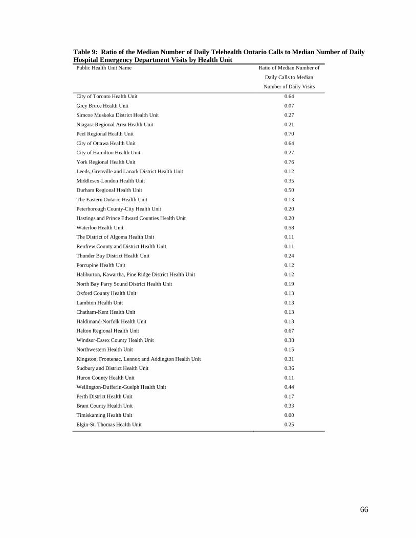
66
Table 9: Ratio of the Median Number of Daily Telehealth Ontario Calls to Median Number of Daily
Hospital Emergency Department Visits by Health Unit Public Health Unit Name Ratio of Median Number of
Daily Calls to Median
Number of Daily Visits
City of Toronto Health Unit 0.64
Grey Bruce Health Unit 0.07
Simcoe Muskoka District Health Unit 0.27
Niagara Regional Area Health Unit 0.21
Peel Regional Health Unit 0.70
City of Ottawa Health Unit 0.64
City of Hamilton Health Unit 0.27
York Regional Health Unit 0.76
Leeds, Grenville and Lanark District Health Unit 0.12
Middlesex-London Health Unit 0.35
Durham Regional Health Unit 0.50
The Eastern Ontario Health Unit 0.13
Peterborough County-City Health Unit 0.20
Hastings and Prince Edward Counties Health Unit 0.20
Waterloo Health Unit 0.58
The District of Algoma Health Unit 0.11
Renfrew County and District Health Unit 0.11
Thunder Bay District Health Unit 0.24
Porcupine Health Unit 0.12
Haliburton, Kawartha, Pine Ridge District Health Unit 0.12
North Bay Parry Sound District Health Unit 0.19
Oxford County Health Unit 0.13
Lambton Health Unit 0.13
Chatham-Kent Health Unit 0.13
Haldimand-Norfolk Health Unit 0.13
Halton Regional Health Unit 0.67
Windsor-Essex County Health Unit 0.38
Northwestern Health Unit 0.15
Kingston, Frontenac, Lennox and Addington Health Unit 0.31
Sudbury and District Health Unit 0.36
Huron County Health Unit 0.11
Wellington-Dufferin-Guelph Health Unit 0.44
Perth District Health Unit 0.17
Brant County Health Unit 0.33
Timiskaming Health Unit 0.00
Elgin-St. Thomas Health Unit 0.25

67
Table 10: Ages of Individuals Telehealth Ontario Calls were Concerning and Ages of Emergency
Department Visit Patients by Health Unit
Emergency Department Visits Telehealth Ontario Calls
Public Health Unit Patient Age Age of Individual Call was
Concerning
Median (75th Percentile,
25th Percentile)
Median (75th Percentile,
25th Percentile)
City of Toronto Health Unit 21 (3, 51) 5 (1, 30)
Grey Bruce Health Unit 30 (9, 52) 7 (1, 30)
Simcoe Muskoka District Health Unit 24 (4, 48) 5 (1, 30)
Niagara Regional Area Health Unit 26 (5, 49) 6 (1, 31)
Peel Regional Health Unit 11 (2, 11) 4 (1, 25)
City of Ottawa Health Unit 19 (3, 49) 5 (1, 28)
City of Hamilton Health Unit 25 (5, 49) 5 (1, 28)
York Regional Health Unit 18 (3, 18) 3 (1, 23)
Leeds, Grenville and Lanark District Health
Unit
27 (7, 27) 7 (1, 31)
Middlesex-London Health Unit 18 (3, 18) 7 (1, 28)
Durham Regional Health Unit 20 (3, 20) 4 (1, 27)
The Eastern Ontario Health Unit 27 (7, 27) 6 (1, 30)
Peterborough County-City Health Unit 30 (10, 52) 13 (2, 31)
Hastings and Prince Edward Counties Health
Unit
27 (7, 49) 6 (1, 29)
Waterloo Health Unit 22 (3, 46) 6 (1, 28)
The District of Algoma Health Unit 28 (9, 51) 10 (2, 32)
Renfrew County and District Health Unit 27 (6, 49) 6 (1, 27)
Thunder Bay District Health Unit 22 (5, 46) 8 (2, 29)
Porcupine Health Unit 27 (6, 49) 9 (2, 29)
Haliburton, Kawartha, Pine Ridge District
Health Unit
30 (8, 53) 10 (2, 35)
North Bay Parry Sound District Health Unit 28 (7, 52) 8 (2, 31)
Oxford County Health Unit 24 (5, 45) 5 (1, 28)
Lambton Health Unit 26 (7, 48) 7 (1, 30)
Chatham-Kent Health Unit 23 (5, 46) 5 (1, 27)
Haldimand-Norfolk Health Unit 21 (5, 46) 6 (1, 29)
Halton Regional Health Unit 16 (2, 44) 3 (1, 26)
Windsor-Essex County Health Unit 22 (3, 50) 3 (1, 25)
Northwestern Health Unit 22 (4, 45) 8 (1, 30)
Kingston, Frontenac, Lennox and Addington
Health Unit
27 (6, 51) 10 (1, 30)
Sudbury and District Health Unit 30 (6, 56) 6 (2, 28)
Huron County Health Unit 28 (6, 53) 6 (1, 31)
Wellington-Dufferin-Guelph Health Unit 22 (4, 44) 5 (1, 28)
Perth District Health Unit 20 (4, 46) 6 (1, 27)
Brant County Health Unit 23 (5, 47) 5 (1, 27)
Timiskaming Health Unit 33 (13, 52) 19 (3, 34)
Elgin-St. Thomas Health Unit 19 (3, 44) 5 (1, 26)

68
4.2 Plots of Daily Calls and Daily Visits over Study Period
Figure 9 and Figure 10 show plots of the daily number of emergency department visits
and Telehealth Ontario calls for respiratory complaints for the approximate City of
Toronto Health Unit and the approximate Grey Bruce Health Unit over the study period
from June 1, 2004 to March 31, 2006.

69
Figure 9: Plot of the Daily Number of Emergency Department Visits and Telehealth Ontario Calls
for Respiratory Complaints for the Approximate City of Toronto Health Unit from June 1, 2004 to
March 31, 2006

70
Figure 10: Plot of the Daily Number of Emergency Department Visits and Telehealth Ontario Calls
for Respiratory Complaints for the Approximate Grey Bruce Health Unit from June 1, 2004 to
March 31, 2006
71
4.3 Qualitative Forecast Assessment
Figure 11 and Figure 13 show the predicted emergency department visits using each of
the three forecasting methods for zero days in the future (i.e. using calls to predict the
current number of visits) for the approximate City of Toronto Health Unit and the
approximate Grey Bruce Health Unit respectively over the validation dataset (days 302 to
669, or March 29, 2005 to March 31, 2006). Note that the time scale in these plots is with
respect to a reference of June 1, 2004 being day 1, and therefore the actual dates of
plotted values can be determined by adding the independent axis value less one to this
reference date. Days that were coded as weekends or statutory holidays (discussed in
section 3.6) are indicated at the bottom of the plots. Figure 12 and Figure 14 show plots
of the corresponding forecasting errors, with positive error indicating forecasts that are
too high and negative errors indicating forecasts that are too low. A zero-days-ahead
forecast is presented as a reference point, as it will be later shown that forecasting error
generally increases with lead time.
Figure 15 through Figure 18 show the same thing for a five-day-ahead forecast rather than
a zero-day-ahead forecast.

72
Figure 11: Zero-Day Ahead Emergency Department Visit Forecast for Respiratory Complaints over
the Validation Dataset for the (Approximate) City of Toronto Health Unit (using all three Forecasting
Methods)

73
Figure 12: Forecasting Errors (Predicted - Actual) for Zero-Day Ahead Emergency Department
Visit Prediction for Respiratory Complaints over the Validation Dataset for the (Approximate) City
of Toronto Health Unit

74
Figure 13: Zero-Day-Ahead Emergency Department Visit Forecast for Respiratory Complaints over
the Validation Dataset for the (Approximate) Grey Bruce Health Unit (using all three Forecasting
Methods)

75
Figure 14: Forecasting Errors (Predicted - Actual) for Zero-Day Ahead Emergency Department
Visit Prediction for Respiratory Complaints over the Validation Dataset for the (Approximate) Grey
Bruce Health Unit

76
Figure 15: Five-Day-Ahead Emergency Department Visit Forecast for Respiratory Complaints over
the Validation Dataset for the (Approximate) City of Toronto Health Unit (using all three Forecasting
Methods)

77
Figure 16: Forecasting Errors (Predicted - Actual) for Five-Day Ahead Emergency Department Visit
Prediction for Respiratory Complaints over the Validation Dataset for the (Approximate) City of
Toronto Health Unit

78
Figure 17: Five-Day-Ahead Emergency Department Visit Forecast for Respiratory Complaints over
the Validation Dataset for the (Approximate) Grey Bruce Health Unit (using all three Forecasting
Methods)
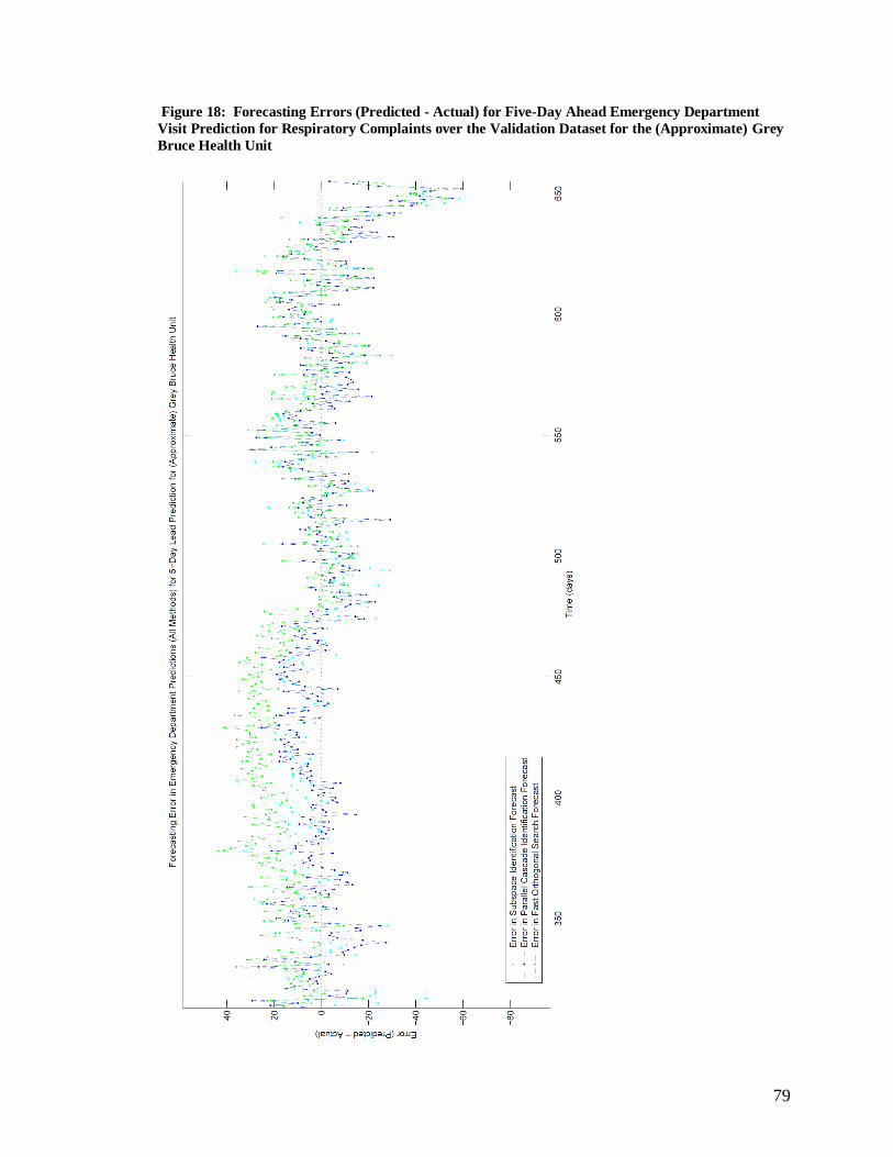
79
Figure 18: Forecasting Errors (Predicted - Actual) for Five-Day Ahead Emergency Department
Visit Prediction for Respiratory Complaints over the Validation Dataset for the (Approximate) Grey
Bruce Health Unit

80
Plots of the forecasted aggregate weekly hospital emergency department visits one week
in advance (aggregate of the forecasted visits for 1-7 days in advance) and two weeks in
advance (aggregate of the forecasted visits for 8-14 days in advance) for the City of
Toronto Health Unit and the Grey Bruce Health Unit are given in Figure 19 through
Figure 22 respectively. These plots better show the trends in the actual and forecasted
time series than do plots of the daily visits.
Appendix C provides plots for the forecasted aggregate weekly hospital emergency
department visits one week in advance for each of the 36 health units.

81
Figure 19: One-Week-Ahead Forecasts of the Weekly Aggregate Number of Hospital Emergency
Visits using all Three Forecasting Methods and the Corresponding Weekly Aggregate Number of
Actual Visits for the (Approximate) City of Toronto Health Unit

82
Figure 20: Two-Week-Ahead Forecasts of the Weekly Aggregate Number of Hospital Emergency
Visits using all Three Forecasting Methods and the Corresponding Weekly Aggregate Number of
Actual Visits for the (Approximate) City of Toronto Health Unit

83
Figure 21: One-Week-Ahead Forecasts of the Weekly Aggregate Number of Hospital Emergency
Visits using all Three Forecasting Methods and the Corresponding Weekly Aggregate Number of
Actual Visits for the (Approximate) Grey Bruce Health Unit

84
Figure 22: Two-Week-Ahead Forecasts of the Weekly Aggregate Number of Hospital Emergency
Visits using all Three Forecasting Methods and the Corresponding Weekly Aggregate Number of
Actual Visits for the (Approximate) Grey Bruce Health Unit

85
4.4 Quantitative Forecast Assessment
Summary statistics for the error in the daily forecasts over the validation dataset for the
City of Toronto Health Unit and the Grey Bruce Health Unit for each of the methods are
given in Table 11 and Table 12 respectively. Summary statistics for the error in the
aggregate weekly forecasts over the validation dataset for these two health units are given
in Table 13 and Table 14. Note in these tables the interquartile range is generally less for
models developed using the Fast Orthogonal Search or Parallel Cascade Identification
methods. Specifically in the case of the Toronto Health Unit, the models developed using
Fast Orthogonal Search had the lowest interquartile range (with some exceptions where
the Subspace models had a lower interquartile range). In the case of the Grey Bruce
Health Unit, the models developed with Parallel Cascade Identification generally had the
lowest interquartile range (with some exceptions where the Subspace models had a lower
interquartile range).

86
Table 11: Summary Statistics of the Error (Predicted-Actual) in Daily Forecasts for the
(Approximate) City of Toronto Health Unit over the Validation Dataset
Parallel Cascade Identification Fast Orthogonal Search Subspace Identification
Lead Median (25th Percentile,
75th Percentile)
Median (25th Percentile,
75th Percentile)
Median (25th Percentile,
75th Percentile)
0 -5 (-15, 4) -2 (-11, 5) -2 (-15, 9)
1 -4 (-14, 5) 0 (-9, 9) -2 (-13, 9)
2 -5 (-14, 5) -1 (-9, 9) -1 (-13, 10)
3 -5 (-13, 5) -2 (-11, 6) -2 (-12, 10)
4 -2 (-11, 8) -2 (-11, 6) 0 (-12, 10)
5 0 (-11, 8) 1 (-10, 9) -3 (-14, 8)
6 0 (-10, 11) 5 (-6, 15) -2 (-13, 10)
7 2 (-9, 12) 4 (-7, 13) -1 (-14, 11)
8 2 (-11, 12) 7 (-4, 17) 0 (-11, 10)
9 2 (-11, 13) 6 (-5, 17) 0 (-13, 11)
10 5 (-8, 15) 5 (-6, 15) 0 (-14, 15)
11 4 (-9, 18) 3 (-9, 11) 2 (-21, 20)
12 4 (-9, 18) 3 (-9, 12) 2 (-15, 16)
13 4 (-10, 16) 11 (-2, 22) 2 (-19, 17)
14 5 (-10, 16) 11 (-3, 22) 1 (-17, 20)
Table 12: Summary Statistics of the Error (Predicted-Actual) in Daily Forecasts for the
(Approximate) Grey Bruce Health Unit over the Validation Dataset
Parallel Cascade Identification Fast Orthogonal Search Subspace Identification
Lead Median (25th Percentile,
75th Percentile)
Median (25th Percentile,
75th Percentile)
Median (25th Percentile,
75th Percentile)
0 0 (-8, 8) 17 (3, 26) 1 (-6, 8)
1 0 (-6, 8) 9 (-5, 18) 10 (-1, 19)
2 0 (-7, 8) 9 (-5, 17) 2 (-6, 9)
3 0 (-7, 8) 9 (-5, 17) 2 (-7, 7)
4 0 (-8, 8) 12 (0, 24) 5 (-5, 13)
5 1 (-8, 9) 11 (0, 22) 4 (-6, 12)
6 1 (-7, 10) 11 (0, 22) 0 (-13, 11)
7 2 (-7, 9) 19 (8, 33) 3 (-6, 11)
8 2 (-6, 10) 21 (8, 34) 5 (-7, 14)
9 2 (-7, 9) 19 (7, 32) 3 (-5, 10)
10 3 (-6, 10) 19 (7, 31) 3 (-6, 10)
11 3 (-6, 11) 1581 (61, 261)
1 3 (-6, 12)
12 4 (-5, 11) 38 (27, 52) 6 (-6, 17)
13 4 (-5, 11) 30 (20, 44) 5 (-7, 13)
14 5 (-6, 12) 17 (5, 35) 7 (-5, 19)
1This model had poor fit over the training data (%MSE > 100%) and should not be used for prediction, explaining this observation

87
Table 13: Summary Statistics of the Error (Predicted-Actual) in the Forecasted Aggregate Number
of Weekly Hospital Emergency Department Visits for Respiratory Illness for the (Approximate) City
of Toronto Health Unit over the Validation Dataset
Parallel Cascade Identification Fast Orthogonal Search Subspace Identification
Weeks
Ahead
Median (25th Percentile,
75th Percentile)
Median (25th Percentile,
75th Percentile)
Median (25th Percentile,
75th Percentile)
1 -5 (-57, 31) 18 (-31, 52) -28 (-70, 42)
2 5 (-66, 97) 48 (0, 97) -17 (-86, 58)
Table 14: Summary Statistics of the Error (Predicted-Actual) in the Forecasted Aggregate Number
of Weekly Hospital Emergency Department Visits for Respiratory Illness for the (Approximate) Grey
Bruce Health Unit over the Validation Dataset
Parallel Cascade Identification Fast Orthogonal Search Subspace Identification
Weeks
Ahead
Median (25th Percentile,
75th Percentile)
Median (25th Percentile,
75th Percentile)
Median (25th Percentile,
75th Percentile)
1 5 (-38, 55) 76 (0, 141) 28 (0, 62)
2 21 (-23, 64) 3231 (259, 382)
1 45 (-21, 84)
1This model had poor fit over the training data (%MSE > 100%) and should not be used for prediction, explaining this observation
The %MSE and MAPE, shown in brackets, of the models over the validation dataset for
leads of 0, 5, 8, 11, and 14 days are given for each of the 36 Ontario health units in Table
15 through Table 19. Results for models with a %MSE of greater than 100% over the
training dataset were excluded from the analysis (indicated by footnotes in the tables).
When %MSE was greater than 100% over the training data, it was deemed that no
suitable forecasting model could be found using that method.

88
Table 15: %MSE (MAPE) for 0-Day-Ahead Forecasts of Hospital Emergency Department Visits for
Respiratory Illness for Each of the 36 Health Units in Ontario over the Validation Dataset 0-Day Lead
Approximate Public Health Region
Parallel Cascade
Identification
Fast Orthogonal
Search
Subspace
Identification
City of Toronto Health Unit 40 (14) 36 (14) 48 (19)
Grey Bruce Health Unit 42 (56) 135 (56) 39 (23)
Simcoe Muskoka District Health Unit 39 (17) 42 (17) 45 (17)
Niagara Regional Area Health Unit 44 (26) 47 (26) 53 (28)
Peel Regional Health Unit 43 (19) 43 (19) 50 (23)
City of Ottawa Health Unit 39 (20) 41 (20) 42 (21)
City of Hamilton Health Unit 46 (26) 49 (26) 67 (31)
York Regional Health Unit 52 (22) 48 (22) 54 (25)
Leeds Grenville and Lanark District Health Unit 69 (26) 64 (26) 71 (27)
Middlesex-London Health Unit 73 (24) 59 (24) 64 (25)
Durham Regional Health Unit 50 (23) 47 (23) 55 (24)
The Eastern Ontario Health Unit 72 (32) 70 (32) 67 (27)
Peterborough County-City Health Unit 70 (36) 68 (36) 91 (41)
Hastings and Prince Edward Counties Health Unit 55 (30) 50 (30) 52 (32)
Waterloo Health Unit 59 (26) 59 (26) 68 (29)
The District of Algoma Health Unit 88 (30) 71 (30) 79 (32)
Renfrew County and District Health Unit 61 (54) 103 (54) 116 (51)
Thunder Bay District Health Unit 90 (43) 107 (43) 81 (32)
Porcupine Health Unit 68 (43) 72 (43) 123 (47)
Haliburton Kawartha Pine Ridge District Health 85 (37) 87 (37) 91 (38)
North Bay Parry Sound District Health Unit 68 (31) 65 (31) 73 (32)
Oxford County Health Unit 50 (34) 49 (34) 59 (37)
Lambton Health Unit 61 (48) 86 (48) 67 (41)
Chatham-Kent Health Unit 102 (75) 164 (75) 180 (75)
Haldimand-Norfolk Health Unit 60 (42) 62 (42) 59 (40)
Halton Regional Health Unit 61 (27) 56 (27) 65 (28)
Windsor-Essex County Health Unit 91 (46) 82 (46) 100 (51)
Northwestern Health Unit 111 (29) 108 (29) 95 (30)
Kingston Frontenac Lennox and Addington Health Unit 66 (35) 65 (35) 68 (34)
Sudbury and District Health Unit 78 (41) 79 (41) 125 (49)
Huron County Health Unit 69 (56) 71 (56) 71 (53)
Wellington-Dufferin-Guelph Health Unit 68 (47) 66 (47) 86 (50)
Perth District Health Unit 73 –1 77 –
1 82 –
1
Brant County Health Unit 81 –1 76 –
1 84 –
1
Timiskaming Health Unit 128 –1 101 –
1 151 –
1
Elgin-St. Thomas Health Unit 72 –1 75 –
1 78 –
1
Average 67 72 78
1 MAPE is not defined when there are zero visits; refer to section 3.9.1.2

89
Table 16: %MSE (MAPE) for 5-Day-Ahead Forecasts of Hospital Emergency Department Visits for
Respiratory Illness for Each of the 36 Health Units in Ontario over the Validation Dataset 5-Day Lead
Approximate Public Health Region
Parallel Cascade
Identification
Fast Orthogonal
Search
Subspace
Identification
City of Toronto Health Unit 39 (17) 38 (15) 45 (19)
Grey Bruce Health Unit 50 (27) 101 (48) 61 (30)
Simcoe Muskoka District Health Unit 46 (18) 61 (22) 53 (19)
Niagara Regional Area Health Unit 49 (27) 54 (28) 79 (36)
Peel Regional Health Unit 45 (20) 43 (19) 50 (23)
City of Ottawa Health Unit 46 (22) 41 (21) 47 (22)
City of Hamilton Health Unit 51 (28) 52 (28) 72 (34)
York Regional Health Unit 55 (24) 51 (23) 57 (26)
Leeds Grenville and Lanark District Health Unit 68 (28) 82 (34) 80 (29)
Middlesex-London Health Unit 66 (26) 68 (24) 64 (27)
Durham Regional Health Unit 54 (25) 57 (26) 59 (26)
The Eastern Ontario Health Unit 58 (26) 67 (33) 71 (30)
Peterborough County-City Health Unit 70 (36) 78 (39) 92 (42)
Hastings and Prince Edward Counties Health Unit 52 (30) 68 (35) 55 (33)
Waterloo Health Unit 62 (29) 4628 (312) 68 (30)
The District of Algoma Health Unit 100 (34) 100 (38) 88 (32)
Renfrew County and District Health Unit 62 (31) 209 (82) 95 (47)
Thunder Bay District Health Unit 93 (35) 234 (76) 85 (32)
Porcupine Health Unit 65 (38) 64 (41) 68 (40)
Haliburton Kawartha Pine Ridge District Health 83 (29) 86 (29) 90 (38)
North Bay Parry Sound District Health Unit 70 (33) 74 (37) 68 (32)
Oxford County Health Unit 49 (33) 185 (95) 54 (36)
Lambton Health Unit 65 (35) 76 (43) 67 (36)
Chatham-Kent Health Unit 121 (58) 128 (66) 138 (65)
Haldimand-Norfolk Health Unit 67 (43) 64 (42) 67 (44)
Halton Regional Health Unit 57 (27) 57 (29) 109 (40)
Windsor-Essex County Health Unit 98 (52) 88 (50) 103 (53)
Northwestern Health Unit 115 (32) 165 (50) 183 (51)
Kingston Frontenac Lennox and Addington Health Unit 64 (37) 68 (41) 66 (36)
Sudbury and District Health Unit 76 (42) 79 (44) 83 (42)
Huron County Health Unit 66 (50) 70 (54) 65 (46)
Wellington-Dufferin-Guelph Health Unit 69 (48) 66 (48) 76 (48)
Perth District Health Unit 82 –1 83 –
1 95 –
1
Brant County Health Unit 75 –1 78 –
1 77 –
1
Timiskaming Health Unit 122 –1 98 –
1 152 –
1
Elgin-St. Thomas Health Unit 83 –1 86 –
1 183 –
1
Average 69 212 82
1 MAPE is not defined when there are zero visits; refer to section 3.9.1.2
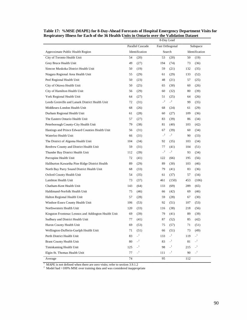
90
Table 17: %MSE (MAPE) for 8-Day-Ahead Forecasts of Hospital Emergency Department Visits for
Respiratory Illness for Each of the 36 Health Units in Ontario over the Validation Dataset 8-Day Lead
Approximate Public Health Region
Parallel Cascade
Identification
Fast Orthogonal
Search
Subspace
Identification
City of Toronto Health Unit 54 (20) 53 (20) 50 (19)
Grey Bruce Health Unit 49 (27) 194 (74) 73 (36)
Simcoe Muskoka District Health Unit 50 (19) 59 (21) 132 (35)
Niagara Regional Area Health Unit 55 (29) 61 (29) 133 (52)
Peel Regional Health Unit 50 (23) 48 (21) 57 (25)
City of Ottawa Health Unit 50 (25) 65 (30) 60 (26)
City of Hamilton Health Unit 56 (29) 60 (32) 80 (39)
York Regional Health Unit 64 (27) 51 (25) 64 (26)
Leeds Grenville and Lanark District Health Unit 72 (31) –2 –
2 99 (35)
Middlesex-London Health Unit 68 (26) 68 (24) 61 (29)
Durham Regional Health Unit 61 (28) 60 (27) 109 (36)
The Eastern Ontario Health Unit 57 (27) 83 (39) 86 (34)
Peterborough County-City Health Unit 79 (38) 81 (40) 103 (42)
Hastings and Prince Edward Counties Health Unit 56 (31) 67 (39) 60 (34)
Waterloo Health Unit 66 (31) –2 –
2 90 (33)
The District of Algoma Health Unit 104 (34) 92 (35) 103 (34)
Renfrew County and District Health Unit 59 (31) 77 (41) 104 (51)
Thunder Bay District Health Unit 112 (39) –2 –
2 93 (34)
Porcupine Health Unit 72 (41) 122 (66) 195 (56)
Haliburton Kawartha Pine Ridge District Health 89 (29) 89 (30) 103 (46)
North Bay Parry Sound District Health Unit 68 (33) 79 (41) 83 (36)
Oxford County Health Unit 54 (35) 61 (37) 57 (34)
Lambton Health Unit 73 (37) 461 (150) 453 (106)
Chatham-Kent Health Unit 143 (64) 133 (69) 289 (65)
Haldimand-Norfolk Health Unit 75 (46) 66 (42) 69 (46)
Halton Regional Health Unit 57 (28) 59 (28) 67 (30)
Windsor-Essex County Health Unit 106 (53) 92 (51) 107 (53)
Northwestern Health Unit 120 (33) 116 (38) 218 (56)
Kingston Frontenac Lennox and Addington Health Unit 69 (39) 79 (41) 89 (39)
Sudbury and District Health Unit 77 (41) 87 (52) 85 (42)
Huron County Health Unit 69 (53) 75 (57) 71 (51)
Wellington-Dufferin-Guelph Health Unit 71 (51) 66 (51) 73 (49)
Perth District Health Unit 83 –1 133 –
1 119 –
1
Brant County Health Unit 80 –1 83 –
1 81 –
1
Timiskaming Health Unit 125 –1 98 –
1 215 –
1
Elgin-St. Thomas Health Unit 77 –1 111 –
1 90 –
1
Average 74 95 112
1 MAPE is not defined when there are zero visits; refer to section 3.9.1.2
2 Model had >100% MSE over training data and was considered inappropriate

91
Table 18: %MSE (MAPE) for 11-Day-Ahead Forecasts of Hospital Emergency Department Visits
for Respiratory Illness for Each of the 36 Health Units in Ontario over the Validation Dataset 11-Day Lead
Approximate Public Health Region
Parallel Cascade
Identification
Fast Orthogonal
Search
Subspace
Identification
City of Toronto Health Unit 50 (21) 45 (17) 92 (30)
Grey Bruce Health Unit 54 (28) –2 –
2 60 (30)
Simcoe Muskoka District Health Unit 56 (21) 113 (37) 71 (23)
Niagara Regional Area Health Unit 60 (32) 82 (38) 63 (30)
Peel Regional Health Unit 52 (24) 53 (21) 95 (35)
City of Ottawa Health Unit 61 (28) 57 (26) 57 (26)
City of Hamilton Health Unit 63 (31) 83 (41) 72 (31)
York Regional Health Unit 59 (27) 55 (26) 66 (26)
Leeds Grenville and Lanark District Health Unit 73 (32) 106 (45) 97 (34)
Middlesex-London Health Unit 70 (26) 69 (25) 71 (27)
Durham Regional Health Unit 69 (30) 63 (28) 87 (32)
The Eastern Ontario Health Unit 62 (29) 113 (49) 81 (35)
Peterborough County-City Health Unit 91 (40) 83 (41) 162 (51)
Hastings and Prince Edward Counties Health Unit 61 (33) –2 –
2 83 (38)
Waterloo Health Unit 71 (34) 206 (78) 70 (30)
The District of Algoma Health Unit 104 (34) 114 (43) 108 (35)
Renfrew County and District Health Unit 63 (33) 98 (51) 99 (48)
Thunder Bay District Health Unit 129 (42) –2 –
2 116 (35)
Porcupine Health Unit 77 (42) 78 (46) 76 (41)
Haliburton Kawartha Pine Ridge District Health 96 (30) 92 (32) 94 (36)
North Bay Parry Sound District Health Unit 68 (33) 99 (52) 77 (32)
Oxford County Health Unit 58 (36) 77 (42) 56 (34)
Lambton Health Unit 76 (38) 100 (60) 81 (51)
Chatham-Kent Health Unit 163 (69) 138 (75) 181 (69)
Haldimand-Norfolk Health Unit 76 (47) 72 (46) 80 (44)
Halton Regional Health Unit 54 (28) 56 (29) 110 (40)
Windsor-Essex County Health Unit 122 (58) 105 (57) 114 (55)
Northwestern Health Unit 126 (34) 118 (38) 143 (43)
Kingston Frontenac Lennox and Addington Health Unit 73 (42) 90 (49) 98 (44)
Sudbury and District Health Unit 80 (42) 116 (69) 90 (44)
Huron County Health Unit 67 (51) 91 (68) 89 (64)
Wellington-Dufferin-Guelph Health Unit 79 (54) 72 (54) 77 (51)
Perth District Health Unit 89 –1 99 –
1 93 –
1
Brant County Health Unit 79 –1 87 –
1 85 –
1
Timiskaming Health Unit 116 –1 110 –
1 147 –
1
Elgin-St. Thomas Health Unit 93 –1 101 –
1 97 –
1
Average 79 92 93
1 MAPE is not defined when there are zero visits; refer to section 3.9.1.2
2 Model had >100% MSE over training data and was considered inappropriate

92
Table 19: %MSE (MAPE) for 14-Day-Ahead Forecasts of Hospital Emergency Department Visits
for Respiratory Illness for Each of the 36 Health Units in Ontario over the Validation Dataset 14-Day Lead
Approximate Public Health Region
Parallel Cascade
Identification
Fast Orthogonal
Search
Subspace
Identification
City of Toronto Health Unit 52 (22) 58 (25) 85 (30)
Grey Bruce Health Unit 60 (30) 195 (71) 87 (43)
Simcoe Muskoka District Health Unit 61 (22) –2 –
2 73 (23)
Niagara Regional Area Health Unit 68 (36) 87 (44) 106 (43)
Peel Regional Health Unit 54 (24) 58 (23) 96 (34)
City of Ottawa Health Unit 63 (29) 86 (38) 62 (27)
City of Hamilton Health Unit 72 (34) 85 (41) 67 (31)
York Regional Health Unit 59 (28) 59 (28) 76 (31)
Leeds Grenville and Lanark District Health Unit 79 (35) 88 (35) 123 (40)
Middlesex-London Health Unit 71 (26) 77 (25) 72 (29)
Durham Regional Health Unit 69 (32) 65 (32) 71 (32)
The Eastern Ontario Health Unit 64 (30) 102 (45) 77 (32)
Peterborough County-City Health Unit 105 (44) 100 (44) 103 (42)
Hastings and Prince Edward Counties Health Unit 68 (36) 96 (49) 95 (42)
Waterloo Health Unit 80 (36) –2 –
2 82 (34)
The District of Algoma Health Unit 124 (38) 113 (43) 101 (35)
Renfrew County and District Health Unit 62 (34) 119 (60) 78 (41)
Thunder Bay District Health Unit 134 (44) –2 –
2 107 (33)
Porcupine Health Unit 91 (44) 108 (58) 138 (65)
Haliburton Kawartha Pine Ridge District Health 95 (31) 95 (32) 93 (33)
North Bay Parry Sound District Health Unit 72 (36) –2 –
2 75 (35)
Oxford County Health Unit 64 (39) –2 –
2 78 (43)
Lambton Health Unit 79 (38) 104 (61) 76 (45)
Chatham-Kent Health Unit 179 (72) 177 (76) 408 (75)
Haldimand-Norfolk Health Unit 80 (49) 69 (46) 104 (63)
Halton Regional Health Unit 54 (28) 56 (29) 70 (31)
Windsor-Essex County Health Unit 130 (59) 110 (59) 113 (53)
Northwestern Health Unit 110 (31) 98 (32) 129 (40)
Kingston Frontenac Lennox and Addington Health Unit 75 (42) 85 (47) 81 (39)
Sudbury and District Health Unit 87 (43) 112 (64) 95 (48)
Huron County Health Unit 71 (52) 95 (78) 100 (73)
Wellington-Dufferin-Guelph Health Unit 87 (58) 71 (52) 83 (55)
Perth District Health Unit 96 –1 92 –
1 116 –
1
Brant County Health Unit 82 –1 87 –
1 80 –
1
Timiskaming Health Unit 128 –1 110 –
1 159 –
1
Elgin-St. Thomas Health Unit 90 –1 147 –
1 91 –
1
Average 84 97 101
1 MAPE is not defined when there are zero visits; refer to section 3.9.1.2
2 Model had >100% MSE over training data and was considered inappropriate

93
An informal comparison of the forecasting accuracy for the three different methods and
the effect of lead time on forecasting accuracy can be made by looking at the ―Average‖
row at the bottom of each table. To formally compare the performance of the different
methods of forecasting visits, and examine the effect of lead time on forecasting
accuracy, a multi-level regression model was used to fit the transformed MSE. The
transformation was chosen to normalize the distribution of the residuals of the regression
model. The following power transformation was used for the %MSE:
1
1100
%1
MSE
MSET
Equation 4-1
MSET was modeled as a function of the prediction lead time in days and prediction
method, both treated as fixed effects. Health Unit was treated as a random effect in the
model to allow for the differences in the health units. Specifically, the multilevel
regression model was:

94
ijijijijjijT PCIFOSleadMSE 3210 (level 1—individual prediction
model)
jjj ratio 400 (level 2—health unit)
),0(~2
Nj
),0(~ 2 N
Equation 4-2
where
the subscript j is used to denote the jth health unit
the subscript i is the ith observation (for a prediction model) in health unit j
lead is the lead time of the predictor in days (0 through 14 days)
FOS is an indicator variable for the Fast Orthogonal Search algorithm (1 if the
prediction model used FOS, 0 otherwise)
PCI is an indicator variable for the Parallel Cascade Identification algorithm (1 if
the prediction model used PCI, 0 otherwise)
ratio is the ratio of the median number of daily calls to median number of daily
visits
β0 is the overall intercept
β1, β2, β3, β4 are the regression coefficients for lead, FOS, PCI and ratio
respectively
αj describes the variation attributable to the health unit
ε describes the unexplained variation in MSET

95
Observations where the MSE exceeded 100% over the training data were excluded from
the regression analysis (a total of 27 observations were excluded—all from Fast
Orthogonal Search); therefore the model was estimated from a total of 1593 observations
(each corresponding to a prediction model; 36 health units × 3 methods × 15 leads (0 to
14 days) – 27 excluded observations).
Table 20: Parameter Estimates for the Multilevel Regression Model of Transformed %MSE, MSET Variable (Coefficient) Parameter Estimate Standard Error p-value
Intercept (β0) 0.9884 0.000796 <0.0001
Prediction lead time (days) (β1) 0.000263 0.000024 <0.0001
Ratio of Median Number of Daily Calls to Median Number of Daily
Visits (β4)
-0.01030 0.002225 <0.0001
Method Subspace (SS) Identification referent n/a n/a
Fast Orthogonal Search (FOS) (β2) -0.00097 0.000277 0.0005
Parallel Cascade Identification (PCI) (β3) -0.00205 0.000275 <0.0001
Covariance Parameters σα2
7.112×10⁻⁶
σ2
5.646×10⁻⁶
This analysis indicates that %MSE increases with prediction lead in days. In terms of
forecasting accuracy as measured by %MSE, Parallel Cascade Identification produced the
most accurate forecasts followed by Fast Orthogonal Search and Subspace Identification.
A model including the interaction between method and lead found these interaction terms
not to be statistically significant. The covariance parameter estimates suggest about 55%
of the total unexplained variation is attributable to differences in health units.
To provide a visual interpretation of the results of the multilevel regression model, plots
of the model estimates for the %MSE for each of the forecasting methods for several
values of the ratio of the median number of daily calls to the median number of daily
visits are given in Figure 23 to Figure 25. This was done as it can be difficult to interpret
the regression coefficients as the dependent variable in the model is the transformed

96
%MSE--the corresponding equation for %MSE is nonlinear. In these plots, three
different values of the ratio of the median number of daily calls to median number of
daily visits is given: 0.6, 0.3, and 0.1. These values were chosen based on the range of
the calls-to-visits ratio given in Table 9.
Figure 23: Regression Model Estimates for the %MSE versus Prediction Lead for Each Forecasting
Method for a Ratio of Median Daily Number of Calls to Median Daily Number of Visits of 0.6
REGRESSION MODEL ESTIMATES FOR
%MSE VERSUS PREDICTION LEAD BY FORECAST METHOD
(CALL-TO-VISITS RATIO OF 0.6)
40
50
60
70
80
90
100
0 2 4 6 8 10 12 14
Prediction Lead (Days)
%M
SE
Parallel Cascade Identification
Fast Orthogonal Search
Subspace Identification

97
Figure 24: Regression Model Estimates for the %MSE versus Prediction Lead for Each Forecasting
Method for a Ratio of Median Daily Number of Calls to Median Daily Number of Visits of 0.3
REGRESSION MODEL ESTIMATES FOR
%MSE VERSUS PREDICTION LEAD BY FORECAST METHOD
(CALL-TO-VISITS RATIO OF 0.3)
40
50
60
70
80
90
100
0 2 4 6 8 10 12 14
Prediction Lead (Days)
%M
SE
Parallel Cascade Identification
Fast Orthogonal Search
Subspace Identification

98
Figure 25: Regression Model Estimates for the %MSE versus Prediction Lead for Each Forecasting
Method for a Ratio of Median Daily Number of Calls to Median Daily Number of Visits of 0.1
REGRESSION MODEL ESTIMATES FOR
%MSE VERSUS PREDICTION LEAD BY FORECAST METHOD
(CALL-TO-VISITS RATIO OF 0.1)
40
50
60
70
80
90
100
0 2 4 6 8 10 12 14
Prediction Lead (Days)
%M
SE
Parallel Cascade Identification
Fast Orthogonal Search
Subspace Identification
4.5 Ability to Predict Increases
Figure 26 illustrates an example of analyses carried out of the ability to predict increases
in emergency department visits above a certain threshold. This example is for the City of
Toronto Health Unit for a seven-day window size and a threshold of 0% (i.e.
discrimination between visit increases/decreases). It was desired to predict increases
above this threshold one week in advance.
The information in this plot is as follows.

99
The validation data set is divided into windows as indicated by the vertical yellow lines.
The actual daily number of emergency visits is shown in red at the bottom of the plot.
The forecasted number of daily visits is plotted in green at the bottom of the plot. The
daily forecasted number of visits time series shown in each window is constructed using
the 1-day-ahead predictor through 7-day-ahead predictor as discussed in 3.9.1.1. The 1-
day-ahead prediction is the left-most point in the window and actually lies on the vertical
yellow line indicating the left boundary of the window. The 2-day-ahead prediction is the
second-from-the-left point in the window, and so on. Days that were holidays or
weekends are given at the bottom of the plot.
The horizontal red bars indicate the aggregate number of actual visits for a given window.
This is the sum of each of the daily visits over that window including the visit that falls on
the left boundary of the window, but not including that on the right side of the window.
The horizontal green bar indicates sum of the forecasted daily visits (generated as
discussed above) over that window. Note that the level of these bars in Figure 26 can be
directly compared to the points plotted in Figure 19.
If the actual aggregate number of visits for the current window exceeds the threshold
percentage increase relative to the baseline window then the window is flagged. In the
case of Figure 26, the baseline window is the immediately preceding window. The
procedure is repeated for the forecasted series. Flagged windows are indicated by an ―×‖
at the top of the plot: red ―×‖s indicate flagged windows for the actual time series, while
lower placed green ―×‖s indicate flagged windows for the forecasted time series.

100
The results of this analysis can be summarized in a two-by-two contingency table
(confusion matrix) giving the number of windows where actual increases were flagged as
increases (true positives), number of windows where actual increases were not flagged
(false negatives), number of windows that were flagged as increases but were not actual
increases (false positives), and number of windows that were not flagged where there was
no actual increase (true negatives). From these tables, the Matthew’s Correlation
Coefficient, sensitivity, specificity, positive predictive value, and negative predictive
value can be calculated with corresponding confidence intervals as discussed in section
3.9.1.3. These results for each of the 36 Ontario Health Units and each of the three
forecasting methods are given in Appendix B for each combination of window size (four-
day or seven-day) and threshold (ability to discriminate between increases and decreases
and nominal thresholds of 10% or 15% increases). It would be overwhelming to present
figures such as Figure 26 for each of these and so the results are presented in tabular
format only.

101
Figure 26: Plot Illustrating Analyses of PCI-Predicted versus Actual Sequence of
Increases/Decreases in Emergency Department Visits One Week in Advance for the City of Toronto
Health Unit

102
4.5.1 Increases in Emergency Visits Aggregated over a Seven Day Window
4.5.1.1 Ability to Discriminate Between Increases and Decreases in the
Aggregate Number of Emergency Visits One and Two Weeks in
Advance
After adjustment for multiple comparisons, none of the predictions for any of the 36
health units showed an ability to discriminate between increases or decreases in the
aggregate number of emergency visits 1-7 or 8-14 days in advance. Table B.1 in
Appendix B presents results for each health unit. The adjustment used the highly
conservative Bonferroni correction, and multiplied each observed p-value by 3 ×36 × 2 =
216 since three methods were tried on 36 PHUs to predict both one- and two-weeks
ahead. Values for Matthew’s Correlation Coefficient, sensitivity, specificity, positive
predictive value, and negative predictive value are reported in the tables when the p-value
for Fisher’s exact test is significant before applying the Bonferroni correction.
Another issue concerned the ability of Telehealth Ontario calls alone to predict increases
and decreases without use of FOS, PCI, or Subspace methods. The lower 95%
confidence intervals for the area under the receiver operating characteristic (AUROC)
were above 0.5 in only four of 72 cases: Niagara Regional Area Health Unit, City of
Ottawa Health Unit, Middlesex-London Health Unit, and Peterborough County-City
Health Unit. In these four cases the lower 95% confidence intervals were very close to
0.5. This provides no evidence for the ability of Telehealth calls to be used directly to

103
discriminate between increases or decreases in aggregate numbers of future emergency
department visits. Table B.2 in Appendix B presents the results for each health unit.
4.5.1.2 Ability to Predict Increases in the Aggregate Number of Future
Visits above a 10% Nominal Threshold One Week in Advance or
a Nominal 15% Threshold Two Weeks in Advance
After adjusting for multiple comparisons (again by the Bonferroni correction), none of the
predictions for any forecasting method for any of the 36 health units showed an ability to
warn of increases in the seven-day aggregate number of emergency visits above a
nominal 10% increase for the next week or above a nominal 15% increase for two weeks
in advance. Table B.3 in Appendix B presents results for each health unit.
The next issue concerned the ability of Telehealth calls alone to predict increases above
this same threshold one- and two-weeks in advance. Six of the 36 health units had lower
95% confidence intervals for area under the receiver operating characteristic that were
above 0.5. Results for the City of Toronto Health Unit indicated that Telehealth Ontario
Calls alone might be predictive of hospital emergency department visits one and two
weeks in advance. Grey Bruce Health Unit, Peel Regional Health Unit, City of Ottawa
Health Unit, Middlesex-London Health Unit, and Durham Region Health Unit had lower
95% confidence intervals AUROC above 0.5. However, this is only seven of 72 cases.
In five of these cases the lower 95% confidence interval was very close to 0.5. Table B.4
in Appendix B presents the results for each health unit.

104
4.5.2 Increases in Emergency Visits Aggregated over Four Day Windows
4.5.2.1 Ability to Discriminate Between Increases and Decreases in the
Aggregate Number of Future Visits over the Next Four Days
Table B.5 in Appendix B presents the results of the ability to discriminate between
increases and decreases in the aggregate number of future visits over the next four days
for each health unit. After conservative adjustment of the p-values for multiple
comparisons, there was evidence for ability to distinguish between increases and
decreases in the aggregate visits for a window consisting of the next four days over a
baseline of the aggregate number of visits over the previous four days in eight of the 36
health units: City of Toronto Health Unit, Peel Regional Health Unit, York Regional
Health Unit, Durham Regional Health Unit, Waterloo Health Unit, Renfrew County and
District Health Unit, Halton Regional Health Unit, and Windsor-Essex County Health
Unit. These results are summarized in Table 21.
Table 21: Health Units where Forecasts Show Ability to Discriminate between Increases and
Decreases in the Aggregate Number of Visits over the Next Four Days Health Unit Best Performing
Method
MCC Sensitivity Specificity PPV NPV
City of Toronto Health Unit FOS 0.68 0.85 0.83 0.85 0.83
Peel Regional Health Unit PCI/FOS
(PCI reported)
0.48 0.77 0.71 0.72 0.76
York Regional Health Unit PCI/SS
(PCI reported)
0.60 0.81 0.78 0.78 0.82
Durham Regional Health Unit PCI 0.46 0.74 0.72 0.71 0.75
Waterloo Health Unit FOS 0.44 0.70 0.74 0.75 0.69
Renfrew County and District Health Unit FOS 0.42 0.70 0.71 0.70 0.71
Halton Regional Health Unit FOS 0.51 0.79 0.72 0.69 0.82
Windsor-Essex County Health Unit FOS/PCI
(PCI reported)
0.51 0.79 0.72 0.72 0.79
Concerning the ability of Telehealth calls alone to predict four-day increases and
decreases, without the use of FOS, PCI, or Subspace methods, only two of the 36 health

105
units had lower 95% confidence intervals for AUROC that were above 0.5: the Eastern
Ontario Health Unit and Huron County Health Unit. Table B.6 in Appendix B presents
the results for each of the 36 health units.
4.5.2.2 Ability to Predict Increases in the Aggregate Number of Future
Visits above a 10% Nominal Threshold over the Next Four Days
Table B.7 in Appendix B presents the results for each health unit. After adjusting for
multiple comparisons and when a nominal threshold of 10% was considered, there was
evidence for ability to flag increases in the aggregate number of future hospital
emergency visits over a period of the next four days compared to the past four days in six
of the 36 health units: City of Toronto Health Unit, Peel Regional Health Unit, York
Regional Health Unit, Durham Regional Health Unit, Halton Regional Health Unit, and
Windsor Essex Health units. A summary of these results is given in Table 22.
Table 22: Health Units where Forecasts Show Ability to Predict 10% Nominal Increases in the
Aggregate Number of Visits over the Next Four Days Health Unit Best Performing
Method
MCC Sensitivity Specificity PPV NPV
City of Toronto Health Unit FOS 0.41 0.54 0.85 0.63 0.80
Peel Regional Health Unit PCI 0.49 0.74 0.77 0.59 0.87
York Regional Health Unit FOS 0.42 0.59 0.82 0.67 0.80
Durham Regional Health Unit PCI 0.46 0.66 0.81 0.66 0.81
Halton Regional Health Unit PCI 0.41 0.69 0.75 0.53 0.85
Windsor-Essex County Health Unit PCI 0.40 0.57 0.75 0.62 0.71
In the case of flagging a nominal 10% increase in visits using Telehealth calls only, the
95% confidence limits for AUROC did not include 0.5 in only two of the 36 health units:
the district of Algoma Health Unit and the Sudbury and District Health Unit. Table B.8
in Appendix B presents the results for each of the 36 health units.

106
Chapter 5 Discussion and Conclusions
5.1 Summary of Key Findings
5.1.1 Forecast Accuracy
This thesis found limited evidence that predictive models employing Telehealth Ontario
Calls and knowledge of upcoming statutory holidays and weekends could be used to
accurately predict future emergency department visits for respiratory illness. Assuming
that it is appropriate to apply the highly conservative Bonferroni correction for multiple
hypothesis testing, then there was no evidence of the ability of such models to accurately
predict increases in the number of weekly emergency department visits either one or two
weeks in advance. However, the Bonferroni correction assumes that each of the multiple
tests is independent and that there is the same probability of obtaining a significant result
in each test. If this were really the case here, then the significant results for individual
tests should occur at random positions in Table B1. In fact, there appears to be a much
greater tendency for significant results to occur near the top of the table, for health units
with larger populations and higher ratios of calls-to-visits. Moreover, the models could
predict increases in the aggregate number of emergency department visits over the next
four days in eight of the health units when discrimination between increases and
decreases was considered and in six of these eight health units when a nominal 10%
threshold was considered even after highly conservative adjustment of p-values. While
six out of 36 health units seems to be a small number, these six health units account for
approximately half of the Ontario population (refer to Table 7). The call-to-visits ratio
was highly correlated with whether a health unit had a significant result or not (in other

107
words these six health units had a significantly higher ratio of calls to visits than the
remaining ones).
Despite the fact that increases were arguably not predicted accurately for the weekly
number of emergency department visits, the forecasts did appear to follow the trend in
these visits for some health units (refer to Figure 19 through Figure 22 and Appendix C).
Unfortunately, plots of both the forecasted and actual time series and the forecasting
errors show that the forecasts sometimes miss important increases in the visits time series
(see for example Figure 15 and Figure 16) which is consistent with the poor ability to
predict increases.
Estimates of the accuracy of the forecasts in terms of the percent mean square error were
not consistent across health units. This is evident in the wide range of values of the mean
square errors in Table 15 through Table 19. This might be expected as the intensity of
Telehealth Ontario call and emergency department visit use had been found to vary
widely by geographic region (3). Some of the variation in the forecast error between
health units was explained by the ratio of the median daily number of calls to the median
daily number of visits as indicated by the results of the multilevel regression model.
Health units with a larger ratio of daily calls-to-visits generally had a lower %MSE.
Analysis of the area under the receiver operating characteristic (AUROC) showed that
Telehealth calls on their own (i.e. without use of a forecasting model) have little or no
ability to predict increases in emergency department visits as most of the confidence
intervals contain 0.50.

108
A lack of consistent ability to predict future increases across health units suggests some
chance findings, in particular for a predictor using only Telehealth calls alone.
5.1.2 Usefulness of Telehealth Ontario Calls versus Knowledge of Upcoming Holidays and Weekends to Predict Future Visits for Respiratory Illness
The prediction models have two independent variables: the number of Telehealth Ontario
calls and an indicator variable for upcoming holiday/weekends. Therefore some of the
ability of such a model to predict increases in hospital emergency department visits is due
to the calls variable and some is due to the weekends/holidays variable. It is well-known
that hospital emergency department visits increase during holidays and weekends (23), so
ability to predict increases based on this knowledge alone would provide little additional
information to those monitoring disease or trying to manage hospital resources.
The fact that prediction accuracy decreases with lead time (i.e. the coefficient for lead
time is statistically significant and greater than zero in the multi-level regression model
used to assess the impact of method and lead time on prediction accuracy) provides
indirect evidence that Telehealth Ontario calls do carry some advance information about
emergency department visits. Longer-lead predictors use Telehealth Ontario call
information further in the past than shorter lead predictors when generating predictions.
However, both longer- and shorter-lead predictors have upcoming weekends/holidays as
far ahead as they are predicting as this information is always available in advance.

109
Therefore, of the two independent variables in the model, only the Telehealth Ontario
calls variable could potentially have less useful information for longer lead predictors.
We would also not expect that the forecasts would follow trends in the visits as shown in
Figure 19 through Figure 22 using only information in an indicator variable for
weekends/holidays.
The fact that, even after applying the Bonferroni correction, predictions of the aggregate
number of visits over a four-day window show accuracy beyond chance for some health
units while predictions of the aggregate number of visits over a seven day window do not
show this suggests two possibilities: 1) that weekend/holiday information is more useful
for predicting visits than call information and/or 2) only accurate short-term forecasts are
possible (i.e. the delay in the conceptual framework in Figure 1 and Figure 2 is short and
calls from longer ago have little use in predicting visits).
5.1.3 Comparison of Forecasting Methods
The coefficients of the indicator variables for modeling method in the multi-level
regression model are all significant suggesting that both the Parallel Cascade
Identification and Fast Orthogonal Search algorithms generally produce more accurate
forecasting models (as measured by %MSE) than the Subspace Identification method.
This finding was further supported by the fact that methods that provided the best ability
to flag increases in the aggregate number of hospital visits (highest MCC) over a four-day

110
period were Parallel Cascade Identification and Fast Orthogonal search (refer to Table 21
and Table 22).
There are two possible reasons why these non-linear methods gave better results than the
subspace method. First, they may have been better able to capture linear information in
the call-to-visits relationship. Second, there may be important nonlinear information in
the call-to-visits relationship which could only be captured using nonlinear modeling
techniques.
5.2 Results in the Context of the Existing Literature
In each of the 36 health units the median patient age of callers for respiratory complaints
was less than the median patient age of patients visiting the emergency department for
respiratory complaints (refer to Table 10). This is consistent with previous research
examining calls and visits at the provincial level (1,4) and supports the conceptual
framework suggested in section 2.5.1.
The fact that Telehealth Ontario calls can be used to generate forecasts of both the daily
and the aggregated number of emergency department visits for respiratory illness that
generally follow the trend in emergency department visits (refer to Figure 19 through
Figure 22) for some of the health units is consistent with the finding by van Dijk et al.
that Telehealth Ontario calls are correlated with emergency department visits at the
provincial level (1). The study by van Dijk found that Telehealth Ontario calls and

111
Emergency Department visits were strongly correlated at a zero day lag and weakly
correlated at up to a 15 day lag. This is consistent with the finding that over all health
units in Ontario, there was a statistically significant decrease in forecasting accuracy with
increasing lead time as discussed in section 5.1.1.
None of the previous literature looked specifically at forecasting hospital emergency
department visits in Ontario or Canada, so there is nothing to directly compare the results
with in terms of forecasting accuracy. However, it is possible to make a general
comparison of the forecasting accuracy for other health services for the five studies
discussed in section 2.3. In order to compare the results obtained in this study with
previous literature, forecasting error must be measured in the same way. Unfortunately,
these five studies did not describe explicitly how the forecasting error they report was
calculated. This makes it difficult to be certain error was measured in the same way it
was in this thesis or to convert the error measurements into the same format. Only the
studies by Reis et al. and Jones et al. are compared below as these are the most relevant in
terms of the health service investigated and because the authors reported enough on the
methods used to make an attempt at comparison feasible.
The study by Reis et al. (39) found an MAPE of 27.5% in forecasts for emergency
department visits for respiratory complaints. Comparing this result (although it is not
possible to make a true comparison) to the MAPE results in Table 15 and Table 16 we
find that the predictions produced by the methods in this thesis are better for some of the
health units than what Reis had found. If the PCI- and FOS-found models perform better
that ARIMA methods, a modified version of the methods used in this thesis might be
valuable in developing models for the expected number of emergency department visits

112
for use in a conventional syndromic surveillance application; the need to do this has been
acknowledged in the syndromic surveillance literature (7).
The study by Jones et al. (28) reported a percent root mean square (%RMS) error of 5.2%
(relative to the mean number of beds occupied) for their forecasting model for bed
occupancy when exogenous inputs were used and 3.2% if no exogenous inputs were used.
It appears that the %RMS error was calculated as:
)(
))()((%
2
ny
nznyRMS
where
y(n) is the actual number of beds occupied
z(n) is the forecasted number of beds occupied
Using the standard deviations in the actual number of beds occupied reported by the
authors, the %RMS errors can be converted into %MSE errors. The %RMS error of 3%
(15.1 beds out of a mean of 441.06 beds with a standard deviation of 32.48 beds) in their
study corresponds to a %MSE of 15.12/32.48
2×100%=21.6% as calculated in this thesis.
The prediction models in Jones et al. therefore may appeared to perform better in that
application as a %MSE of 22% was lower than any of the prediction models in this thesis.
However, note that the authors in their study only test over a validation set consisting of
the next 32 days whereas in this thesis the models are tested over a validation set of
approximately one year. Shorter validation sets make it more likely that the relationship
will not change over the validation set and that better forecasting results will be obtained.

113
5.3 Study Strengths
The study undertaken in this thesis had strengths in terms of quality of the data used to
verify the forecasts, its pragmatic approach to studying the Telehealth call-emergency
department visit relationship, the various measures it used in reporting forecasting errors,
its examination of the call-visits relationship at the health unit level, and the use of several
approaches in establishing a relationship between calls and visits.
The high quality and coverage of the NACRS database (discussed in section 3.4.1) put the
study in a good position to be able to conclude whether forecasts of emergency
department visits for respiratory illness using Telehealth Ontario calls were accurate and
useful. Good measurement of the true number of emergency department visits is
necessary before it is possible to conclude whether or not forecasts are accurate. If only a
poor measurement of the actual number of visits were used, then poor forecasts could
have been due to either the methods used or simply to the fact that measurement of the
truth was inaccurate.
Because this study used a variety of approaches to measure the association between calls
and visits, including those allowing for nonlinearity in this association, there was
increased chance of capturing an association if one existed. The fact that similar results
were obtained by several different approaches to modeling the association reinforces the
study findings about predictive ability of Telehealth and weekend/holiday information.
For example, the models developed by all three forecasting methods generated similar

114
forecasts and errors for the City of Toronto as shown in Figure 11 and Figure 12.
Similarly, measurements of the %MSE and MAPE reported in Table 15 through Table 19
are consistent across the methods for a given health unit relative to other health units.
This study took a pragmatic approach to studying the association between calls and visits:
the association between calls and visits was examined from the point of view of how
knowledge of its existence might be used in a practical application of forecasting future
visits. This is in contrast to previous work in investigating data sources for syndromic
surveillance data that yielded only a correlation coefficient between the data source under
study and a measure of the outcome (1,32,33). Such a pragmatic approach allows the
results of the study to be more easily interpreted in the context of how they may be
applied.
This study quantified the forecasting error in a number of ways including summary
measures of the error, %MSE and MAPE, measurement of the ability to discriminate
between increases and decreases, ability to predict increases above a threshold, and plots
and summary statistics of the errors for select health units. Previous research (discussed
in section 2.3) has reported only summary measures of the error, which can be difficult to
interpret.
The association between calls and visits was investigated at the health unit level allowing
for regional differences in the relationship that might be expected because of differing use
in Telehealth Ontario and emergency department services. Previous work by van Dijk (1)
et al. had only looked at the relationship at the provincial level, although geographical

115
analysis of the intensity of Telehealth Ontario call and emergency department visit use
had been found to vary widely by geographic region (3). This allows the usefulness of
Telehealth calls in each of the health units to be assessed.
5.4 Study Limitations
This thesis had several limitations in terms of how it handled the confounding effect of
holidays/weekends, how it statistically tested the ability of forecasts to predict increases
in visits, its adjustment of the AUROC for multiple comparisons and correlation when
assessing the usefulness of raw Telehealth Ontario calls in making predictions, the small
sample size used in model validation, how it assigned calls and visits to Health Units, and
the assumptions made about the static nature of the Telehealth calls to ED visits
relationship.
Assessment of the ability to predict increases in the aggregate number of visits over a
seven day window was used to control for confounding, specifically the fact that
emergency visits and Telehealth calls are both known to vary on a weekly basis. Some
residual confounding may be present because of the fact that this adjustment does not
account for holidays. With a seven-day window, increase due for example to Christmas
holidays would not be controlled for. Because of this confounding effect, it is difficult to
say whether ability to predict increases over a four day window beyond chance was due
only to the weekend/holiday information presented to the model or to both this
information and the Telehealth call information. Fitting a model that only used
Telehealth call information and comparing it to the performance of a model that used both

116
Telehealth call information and weekend/holiday information would not necessarily
resolve this problem because Telehealth call information implicitly contains information
about holidays/weekends (i.e. there is some collinearity between these variables) since
call volume is known to increase on weekends (5).
The statistical tests to determine whether predicted increases are better than chance
assume that observations are independent of one another as do computation of confidence
intervals for measures of sensitivity, specificity, positive predictive value and negative
predictive value. Note that windows are not necessarily independent of each other
because of autocorrelation in the time series. It is also noted that when the memory
length of the predictors is less than the window size, there will be some correlation
between the predictions. Therefore predictions may not be independent of each other
either. No attempt was made to correct for this. This type of correlation would reduce
the effective sample size and widen the confidence intervals reported for the sensitivity,
specificity, positive predictive value, and negative predictive value. This also would
affect the calculation of the confidence limits for the AUROC in assessing the predictive
value of raw counts of Telehealth Ontario calls for respiratory complaints.
Although the upper and lower 95% confidence intervals for the AUROC are provided, it
could be argued that a one-tailed test is actually more appropriate since we are only
interested in determining whether or not the AUROC is greater than 0.5, and that really
the cutoff to consider the AUROC significant was p=0.025 rather than p=0.05. However,
this is more than offset by the fact that the AUROC is not adjusted for multiple

117
comparisons or for possible correlation in the prediction windows as discussed above.
Therefore it is entirely likely that positive findings were due only to chance.
The confidence intervals for the sensitivity and specificity are wide indicating that one
year of validation data is insufficient to give a good assessment of the predictive ability of
the forecasting models. For example, the sensitivity of the fast orthogonal search forecast
for the City of Toronto Health Unit had a 95% confidence interval of 0.34 to 0.72. It is
difficult to assess in advance how much data is required to train the models to achieve
reasonable fit, and therefore to know how much data will be available for validation. It
was also not known in advance how many increases and non-increases there would be
over the validation data set. This makes calculating sample size and study power very
difficult. The results of this study could therefore be useful in designing future follow-up
studies.
Because only patient forward sortation area is available in the call and visit data and
forward sortation areas do not have a one-to-one correspondence with health units as
discussed in section 3.7, the Health Unit labeling of the geographical groupings in this
study are only approximate. In other words, calls and visits always come from the same
geographic region, but the regions may not exactly represent the health units. If an
individual health unit were interested in applying the results, an analysis would have to be
carried out to determine the overlap in geographical regions.

118
A related issue is that callers from one region may seek care in another region. This
could be particularly problematic where health unit boundaries separate a populated area
from the centre that provides care for that area.
This study assumes that the relationship between calls and visits is time invariant. The
models capture the relationship between calls and visits over the first year of data and
then assume that this remains the same over the second year of data. This may not be the
case, however. For example, call patterns may change due to shifts in behaviour or the
delays between calls and visits may vary depending on the underlying cause of the
respiratory complaints. Better predictive models might be achieved by using triage
information rather than NACRS database information to fit the models. Since this
information is available in real-time, the models could be updated on an on-going basis to
correct for the time-varying nature of the calls-visits relationship.
5.5 Application of Results and Implications for Future Research
The forecasts using Telehealth Ontario calls and the methods presented in this thesis do
not generate forecasts that are accurate enough to be used as a sole means of making
decisions about future increases in the number of emergency department visits for
respiratory illness. However, the models may generate accurate enough predictions at
short leads to be used as a crude proxy for the actual number of emergency department
visits. The plots given in Appendix C provide evidence for this. Even though accurate
flagging of increases only occurs in six of the 36 health units, these health units account

119
for approximately half of the Ontario population (refer to Table 7). This could still allow
the forecasts to contribute valuable information to a surveillance system that incorporates
data from multiple sources. The information provided by the forecasts might be especially
useful because aggregate emergency department visit information at the health unit level
may be difficult, time consuming, and costly to obtain from other sources.
The forecasts generated by the methods discussed in this thesis might be improved if
emergency visits for past days were available. Recall from section 3.8.5 that these were
not assumed to be available to the forecasting system as NACRS data is only available at
the end of the fiscal year. If information collection systems are improved, it is feasible
that such information would be available. This would allow for three things. First, it
would allow the models to be updated on an on-going basis to correct for changes in the
call-to-visits relationship. Doing so would reduce, to some extent, the assumption of a
time invariant relationship discussed in section 5.4 (the length of time over which the
relationship was assumed to be time invariant would be reduced). Second, it would allow
an accurate number of baseline visits to be estimated when predicting increases, possibly
improving accuracy of these predictions. Third, when FOS-found difference equation
models are employed to make predictions, it would allow actual values of past visits to be
used in the models rather than calculated values of past visits.
The methods developed here might be applied to other syndromic surveillance time series
or for forecasting demand for other health services with better success. As stated earlier,
poor forecasts could be due to either: 1) that the methods were inadequate to capture
information in the data that would allow accurate forecasts or 2) that the data used to

120
produce the forecasts does not contain enough information in order to generate accurate
forecasts. Forecasting accuracy of the models might be improved if they incorporate
information from other independent variables. For example, if real-time triage data were
available, this might improve model accuracy.
The threshold approach to flagging increases using the forecasted time series might be
improved by developing a predictor model directly. In other words, instead of outputting
the forecasted number of visits, the predictor might output a binary variable indicating an
increase or no increase. Such predictors have been developed using Parallel Cascade
Identification for other purposes (68).

121
References
(1) van Dijk A, McGuinness D, Rolland E, Moore KM. Can Telehealth Ontario
respiratory call volume be used as a proxy for emergency department respiratory visit
surveillance by public health? CJEM 2008 Jan;10(1):18-24.
(2) Moore K. Real-time syndrome surveillance in Ontario, Canada: the potential use of
emergency departments and Telehealth. Eur.J.Emerg.Med. 2004 Feb;11(1):3-11.
(3) Moore KM. Integrating Ontario’s Telehealth program into a province-wide public
health surveillance system: evaluation and recommendations. 2008.
(4) Rolland E, Moore KM. Ontario's Telehealth: A Novel Syndromic Surveillance Tool.
Advances in Disease Surveillance 2007;4:190-190.
(5) Rolland E, Moore KM, Robinson VA, McGuinness D. Using Ontario's "Telehealth"
health telephone helpline as an early-warning system: a study protocol. BMC Health
Serv.Res. 2006 Feb 15;6:10.
(6) Webb P, Bain C, Pirozzo S. Essential Epidemiology. New York: Cambridge
University Press; 2005.
(7) Buckeridge DL, Burkom H, Campbell M, Hogan WR, Moore AW. Algorithms for
rapid outbreak detection: a research synthesis. Journal of Biomedical Informatics, 2005
4;38(2):99-113.
(8) Kleinman K, Abrams A. Assessing Surveillance Using Sensitivity, Specificity and
Timeliness. Statistical Methods in Medical Research 2006;15:445-464.
(9) Lombardo J, Buckeridge D editors. Disease Surveillance: A Public Health Informatics
Approach. 1st ed. New Jersey: John Wiley & Sons, Inc.; 2007.

122
(10) Naylor D, Basrur S, Bergeron M, Brunham R, Butler-Jones D, Dafoe G, et al.
National Advisory Committee on SARS and Public Health: Learning from SARS:
Renewal of Public Health in Canada. 2003.
(11) Ontario Ministry of Health and Long-Term Care. For The Public's Health : Initial
Report of the Ontario Expert Panel on SARS and Infectious Disease Control. 2003.
(12) Ontario Ministry of Health and Long-Term Care. Ontario Health Pandemic Influenza
Plan June 2005. 2005:68-78.
(13) Walker D, Keon W, Laupacis A, Low D, Moore K, Kitts J, et al. The Ontario Expert
Panel on SARS and Infectious Disease Control: For the Public's Health: A Plan of
Action--Final Report of the Ontario Expert Panel on SARS and Infectious Disease
Control. 2004.
(14) Campbell A. Commission to Investigate the Introduction and Spread of SARS in
Ontario: Interim Report: SARS and Public Health in Ontario. 2004.
(15) Mandl K, Overhage M, Wagner M, Lober W, Sebastiani P, Mostashari F, et al.
Implementing Syndromic Surveillance: A Practical Guide Informed by the Early
Experience. Journal of the American Medical Informatics Association 2004;11(2):141-
150.
(16) Burkom, HS, Murphy, SP, Shmueli G. Automated Time Series Forecasting for
Biosurveillance. Statistics in Medicine 2007;26:4202-4218.
(17) Lombardo J, Burkom H, Elbert E, Magruder S, Lewis S, Loschen W, et al. A
Systems Overview of the Electronic Surveillance System for the Early Notification of
Community-Based Epidemics (ESSENCE II). Journal of Urban Health: Bulletin of the
New York Academy of Medicine 2003;80(2, Supplement 1):i32-i42.
(18) Gostin L. Public Health Strategies for Pandemic Influenza. The Journal of the
American Medical Association 2006;295(14):1700-1704.

123
(19) Kwong J, Rosella L, Johansen H. Trends in influenza vaccination in Canada,
1996/1997 to 2005. Health Reports 2007;18(4):1-11.
(20) Ontario Hospital Association and Ontario Medical Association Joint Committee on
Communicable Disease Surveillance Protocols. Influenza Surveillance Protocol for
Ontario Hospitals. 2005;306.
(21) Eskin B, Levy R. Does This Patient Have Influenza? Annals of Emergency Medicine
2007;49(1):103-105.
(22) Public Health Agency of Canada. Leading Causes of Death and Hospitalization in
Canada. 2008; Available at: http://www.phac-aspc.gc.ca/publicat/lcd-pcd97/index-
eng.php. Accessed 08/01, 2008.
(23) Chan B, Schull MJ, Schultz SE. Atlas Report: Emergency Department Services in
Ontario 1993-2000. 2001.
(24) Brown A, Alikhan M, Anderson G, Baker G, Croxford R, Daniel I, et al. Hospital
Report 2003: Emergency Department Care. 2004.
(25) Menec V, Bruce S, MacWilliam L. Exploring Reasons for Bed Pressures in
Winnipeg Acute Care Hospitals. Canadian Journal of Aging 2005;24(Supplement 1):121-
131.
(26) Menec V, Black C, MacWilliam L, Aoki F. The Impact of Influenza-Associated
Respiratory Illnesses on Hospitalizations, Physician Visits, Emergency Room Visits, and
Mortality. Canadian Journal of Public Health 2003;94(1):59-63.
(27) Hanratty B, Robinson M. Coping with Winter Bed Crises. BMJ 1999;319:1511-
1512.
(28) Jones S, Joy M. Forecasting Demand of Emergency Care. Health Care Management
Science 2002;5:297-305.

124
(29) Huges D, McGuire A. Stochastic Demand, Production Responses and Hospital
Costs. Journal of Health Economics 2003;22:999-1010.
(30) Viberg M. Subspace-based Methods for the Identification of Linear Time-invariant
Systems. Automatica 1995;31(12):1835-1851.
(31) Ontario Ministry of Health and Long-Term Care. Telehealth Ontario. 2006;
Available at:
http://www.health.gov.on.ca/english/public/program/telehealth/telehealth_mn.html.
Accessed 03/21, 2009.
(32) Doroshenko A, Cooper D, Smith G, Gerard E, Chinemana F, Verlander N, et al.
Evaluation of Sydromic Surveillance Based on National Health Service Direct Derived
Data -- England and Wales. Morbidity and Mortality Weekly Report
2005;54(Supplement):117-122.
(33) Zheng W, Aitken R, Muscatello D, Churches T. Potential for early warning of viral
influenza activity in the community by monitoring clinical diagnoses of influenza in
hospital emergency departments. BMC Public Health 2007;7(1):250.
(34) Makridakis S, Wheelwright S, Hyndman R. Forecasting: methods and applications.
3rd ed. New York: Wiley; 1998.
(35) Brockwell P, Davis R. Introduction to Time Series and Forecasting. 2nd ed. New
York: Springer-Verlag; 2002.
(36) Finarelli H, Johnson T. Effective Demand Forecasting in 9 Steps. Healthcare
Financial Management 2004;58(11):52-58.
(37) Abdel-Aal R, Mangoud A. Modeling and Forecasting Monthly Patient Volume at a
Primary Health Care Clinic using Univariate Time-Series Analysis. Computer Methods
and Programs in Biomedicine 1998;56:235-247.

125
(38) Diaz J, Aberdi J, Pajares M, Lopez C, Lopez R, Lage M, et al. A Model for
Forecasting Emergency Hospital Admissions: Effect of Environmental Variables. Journal
of Environmental Health 2001;64(3):15.
(39) Reis B, Mandl K. Time Series Modeling for Syndromic Surveillance. BMC Medical
Informatics and Decision Making 2003;3(2).
(40) Upshur R, Moineddin R, Crighton E, Kiefier L, Mamdani M. Simplicity within
Complexity: Seasonality and Predictability of Hospital Admissions in the Province of
Ontario 1988-2001, A Population-Based Analysis. BMC Health Services Research
2005;5(13).
(41) Crighton E, Moineddin R, Mamdani M, Upshur REG. Influenza and pneumonia
hospitalizations in Ontario: a time-series analysis. Epidemiology and Infection
2004;132:1167-1174.
(42) Marsden-Haug N, Foster V, Gould P, Elbert E, Wang H, Pavlin J. Code-based
Syndromic Surveillance for Influenzalike Illness by International Classification of
Diseases, Ninth Revision. Emerging Infectious Diseases 2007;13(2):207-216.
(43) Mandl K, Lee T. Integrating Medical Informatics and Health Services Research: The
Need for Dual Training at the Clinical Health Systems and Policy Levels. Journal of the
American Medical Informatics Association 2002;9(2):127-132.
(44) Canadian Institute for Health Information. Database Background and General Data
Limitations Documentation: National Ambulatory Care Reporting System (NACRS) FY
2005-2006. 2006.
(45) Canadian Institute for Health Information. Database Background and General Data
Limitations Documentation: National Ambulatory Care Reporting System (NACRS) FY
2004-2005. 2005.
(46) Reyes F, Aziz S, Li Y, Macey J, Winchester B, Garner M, et al. Influenza in Canada:
2006-2007 Season. Canada Communicable Disease Report 2008;34(3):1-25.

126
(47) Ontario Ministry of Health and Long-Term Care. ICD10-CA to ICD-9 Conversion
Table. 2006.
(48) Canadian Institute for Health Information. 2006/2007 Conversion Tables: ICD-10-
CA/CCI to ICD-9-CM (July 2006 Update). 2007.
(49) Canadian Institute for Health Information. CIHI Data Quality Study of Ontario
Emergency Department Visits for Fiscal Year 2004-2005--Executive Summary. 2007.
(50) Ontario Ministry of Health and Long-Term Care. Telehealth Ontario. 2002;
Available at:
http://www.health.gov.on.ca/english/public/program/telehealth/telehealth_mn.html.
Accessed 02/14, 2009.
(51) Statistics Canada. Postal Code Conversion File (PCCF), Reference Guide.
2006;92F0153GIE.
(52) Mechanda K, Puderer H. How Postal Codes Map to Geographic Areas.
2007;92F0138MIE.
(53) Statistics Canada. Health Region Boundary File. 2005.
(54) Statistics Canada. Health Regions: Boundaries and Correspondence with Census
Geography. 2007;82-402-XIE.
(55) Ljung L. From Data to Model: A Guided Tour of System Identification. 1994;LiTH-
ISY-R-1652.
(56) Ljung L. MATLAB System Identification Toolbox User's Guide. Version 6 ed.
Natick, MA: The MathWorks; 2003.
(57) D. Westwick. Methods for the Identification of Multiple-Input Nonlinear
SystemsMcGill University; 1995.

127
(58) Gilbert P. State Space and ARMA Models: An Overview of the Equivalence.
1993;Bank of Canada Working Paper 93-4.
(59) Katayama T. Subspace methods for system identification: a realization approach.
London: Springer-Verlag; 2005.
(60) Overschee P, DeMoor B. N4SID: Subspace Algorithms for the Identification of
Combined Deterministic-Stochastic Systems. Automatica 1994;30(1):75-93.
(61) Korenberg M. A Robust Orthogonal Algorithm for System Identification and Time-
Series Analysis. Biological Cybernetics 1989;60:267-276.
(62) Korenberg M. Identifying Nonlinear Difference Equation and Functional Expansion
Representations: The Fast Orthogonal Algorithm. Annals of Biomedical Engineering
1988;16:123-142.
(63) Desrochers A. On an improved model reduction technique for nonlinear systems.
Automatica 1981;17(2):407-409.
(64) Korenberg M. Parallel Cascade identification and Kernel Estimation for Nonlinear
Systems. Annals of Biomedical Engineering 1991;19:429-455.
(65) Korenberg M, David R, Hunter I, Solomon JE. Parallel Cascade Identification and its
Application to Protein Family Prediction. Journal of Biotechnology 2001;91:35-47.
(66) Korenberg M, Doherty P. Rapid DTMF signal classification via parallel cascade
identification. Electronics Letters 1996;32(20):1862-1863.
(67) Korenberg M, McGaughey D, Aitken G. Parallel cascade prediction of turbulence
induced wavefront tilt. Electronics Letters 1996;32(14):1315-1316.
(68) Korenberg M, Solomon JE, Regelson ME. Parallel Cascade Identification as a
Means for Automatically Classifying Protein Sequences into Structural/Functional
Groups. Biological Cybernetics 2000;82:15-21.

128
(69) Eklund M, Korenberg M. Simulation of Aircraft Pilot Flight Controls Using
Nonlinear System Identification. Simulation 2000;75(2):72-81.
(70) Green J, Korenberg M. On the Advantages of Multi-Input Single-Output Parallel
Cascade Classifiers. Annals of Biomedical Engineering 2006;34(4):709-716.
(71) The MathWorks Inc. MATLAB Version 7 Release 14. 2003.
(72) Minz I, Korenberg M. Modeling Cooperative Gene Regulation Using Fast-
Orthogonal Search. The Open Bioinformatics Journal 2008;2:80-89.
(73) Windhorst U, Johansson H editors. Modern Techniques in Neuroscience Research.
1st ed. New York: Springer; 1999.
(74) Markridakis S, Wheelwright S, McGee V. Forecasting: Methods and Applications.
2nd ed. Toronto: John Wiley & Sons; 1983.
(75) Makridakis S. Accuracy Measures: Theoretical and Practical Concerns. International
Journal of Forecasting 1993;9:527-529.
(76) Goodwin P, Lawton R. On the asymmetry of the symmetric MAPE. International
Journal of Forecasting 1999;15:405-408.
(77) Baldi P, Brunak S, Chauvin Y, Andersen C, Nielsen H. Assessing the Accuracy of
Prediction Algorithms for Classification: An Overview. Bioiinformatics 2000;16(5):412-
424.
(78) Lund O, Nielsen M, Lundegaard C, Kesmir C, Brunak S. Immunological
Bioinformatics. 1st ed. Cambridge, Massachusetts: The MIT Press; 2005.
(79) Bender R, Lange S. Adjusting for multiple testing--when and how? Journal of
Clinical Epidemiology 2001;54:343-349.
(80) Bewick V, Cheek L, Ball J. Statistics review 13: Receiver operating characteristic
curves. Critical Care 2004;8(6):508-512.

129
(81) Park S, Goo J, Jo C. Receiver Operating Characteristic (ROC) Curve: Practical
Review for Radiologists. Korean Journal of Radiology 2004;5(1):11-18.

130
Appendices
APPENDIX A: Ethics Approval

131
APPENDIX B: Ability of Forecasts to Predict Increases in Emergency Department Visits Table B.1: Ability to Discriminate Between Increases and Decreases in Weekly Aggregate Number of Hospital Emergency Department Visits One or
Two Weeks in Advance
TP FN TN FP Point
Estimate
Lower
95% CI
Upper
95% CI
Point
Estimate
Lower
95% CI
Upper
95% CI
Point
Estimate
Lower
95% CI
Upper
95% CI
Point
Estimate
Lower
95% CI
Upper
95% CI
City of Toronto Health Unit 1 FOS 19 10 13 6 0.038 1.000 0.34 0.64 0.44 0.81 0.70 0.46 0.88 0.75 0.53 0.90 0.58 0.37 0.78
City of Toronto Health Unit 1.000 PCI 20 9 14 5 0.007 1.000 0.42 0.68 0.48 0.84 0.75 0.51 0.91 0.79 0.58 0.93 0.63 0.41 0.81
City of Toronto Health Unit 1.000 SS 17 12 9 10 0.770 1.000 0.11 0.61 0.41 0.78 0.50 0.27 0.73 0.63 0.42 0.81 0.48 0.26 0.70
City of Toronto Health Unit 2 FOS 14 10 15 9 0.248 1.000 0.21 0.57 0.34 0.77 0.64 0.43 0.82 0.59 0.36 0.79 0.62 0.41 0.80
City of Toronto Health Unit 2.000 PCI 13 11 12 12 1.000 1.000 0.04 0.52 0.31 0.73 0.52 0.31 0.72 0.50 0.29 0.71 0.54 0.33 0.74
City of Toronto Health Unit 2.000 SS 13 11 11 13 1.000 1.000 0.05 0.57 ed 0.77 0.48 0.28 0.69 0.50 0.30 0.70 0.55 0.32 0.76
Grey Bruce Health Unit 1 FOS 8 13 21 6 0.338 1.000 0.15 0.35 0.15 0.59 0.79 0.59 0.92 0.54 0.25 0.81 0.63 0.45 0.79
Grey Bruce Health Unit 1.000 PCI 12 9 16 11 0.383 1.000 0.16 0.55 0.32 0.77 0.61 0.41 0.78 0.50 0.28 0.72 0.65 0.44 0.83
Grey Bruce Health Unit 1.000 SS 11 10 16 11 0.561 1.000 0.11 0.50 0.27 0.73 0.61 0.41 0.78 0.48 0.26 0.70 0.63 0.42 0.81
Grey Bruce Health Unit 2 FOS* 19 1 11 17 0.008 1.000 0.40 0.95 0.74 1.00 0.41 0.24 0.61 0.51 0.34 0.69 0.92 0.64 1.00
Grey Bruce Health Unit 2.000 PCI 11 9 17 11 0.381 1.000 0.14 0.53 0.29 0.76 0.62 0.42 0.79 0.48 0.26 0.70 0.67 0.46 0.83
Grey Bruce Health Unit 2.000 SS 13 7 14 14 0.382 1.000 0.20 0.68 0.43 0.87 0.52 0.33 0.71 0.48 0.29 0.68 0.71 0.48 0.89
Simcoe Muskoka District Health Unit 1 FOS 13 11 14 10 0.564 1.000 0.12 0.52 0.31 0.73 0.60 0.39 0.79 0.55 0.32 0.76 0.58 0.37 0.77
Simcoe Muskoka District Health Uni 1.000 PCI 13 11 13 11 0.773 1.000 0.08 0.52 0.31 0.73 0.56 0.35 0.76 0.52 0.31 0.73 0.56 0.35 0.76
Simcoe Muskoka District Health Uni 1.000 SS 13 11 14 10 0.564 1.000 0.12 0.52 0.31 0.73 0.60 0.39 0.79 0.55 0.32 0.76 0.58 0.37 0.77
Simcoe Muskoka District Health Uni 2 FOS* 17 5 13 13 0.074 1.000 0.28 0.76 0.53 0.92 0.52 0.32 0.71 0.55 0.36 0.74 0.74 0.49 0.91
Simcoe Muskoka District Health Uni 2.000 PCI 12 10 15 11 0.563 1.000 0.12 0.52 0.30 0.74 0.59 0.39 0.78 0.50 0.28 0.72 0.62 0.41 0.80
Simcoe Muskoka District Health Uni 2.000 SS 11 11 14 12 1.000 1.000 0.03 0.48 0.26 0.70 0.56 0.35 0.75 0.45 0.24 0.68 0.58 0.37 0.77
Niagara Regional Area Health Unit 1 FOS 12 9 17 10 0.244 1.000 0.19 0.55 0.32 0.77 0.64 0.44 0.81 0.52 0.30 0.74 0.67 0.46 0.83
Niagara Regional Area Health Unit 1.000 PCI 10 11 16 11 0.771 1.000 0.06 0.45 0.23 0.68 0.61 0.41 0.78 0.45 0.23 0.68 0.61 0.41 0.78
Niagara Regional Area Health Unit 1.000 SS 9 12 10 17 0.244 1.000 -0.20 0.40 0.19 0.64 0.39 0.22 0.59 0.32 0.15 0.54 0.48 0.27 0.69
Niagara Regional Area Health Unit 2 FOS 12 11 16 9 0.383 1.000 0.16 0.50 0.28 0.72 0.65 0.44 0.83 0.55 0.32 0.77 0.61 0.41 0.78
Niagara Regional Area Health Unit 2.000 PCI 15 8 16 9 0.082 1.000 0.29 0.64 0.41 0.83 0.65 0.44 0.83 0.61 0.39 0.80 0.68 0.46 0.85
Niagara Regional Area Health Unit 2.000 SS 16 7 15 10 0.049 1.000 0.30 0.68 0.45 0.86 0.62 0.41 0.80 0.60 0.39 0.79 0.70 0.47 0.87
Peel Regional Health Unit 1 FOS 13 10 12 13 0.780 1.000 0.05 0.55 0.32 0.76 0.50 0.30 0.70 0.48 0.28 0.69 0.57 0.34 0.77
Peel Regional Health Unit 1.000 PCI 12 11 15 10 0.563 1.000 0.12 0.50 0.28 0.72 0.62 0.41 0.80 0.52 0.30 0.74 0.59 0.39 0.78
Peel Regional Health Unit 1.000 SS 13 10 14 11 0.564 1.000 0.12 0.55 0.32 0.76 0.58 0.37 0.77 0.52 0.31 0.73 0.60 0.39 0.79
Peel Regional Health Unit 2 FOS 17 11 14 6 0.045 1.000 0.31 0.59 0.39 0.78 0.71 0.48 0.89 0.73 0.50 0.89 0.58 0.37 0.77
Peel Regional Health Unit 2.000 PCI 16 12 15 5 0.040 1.000 0.32 0.56 0.35 0.75 0.76 0.53 0.92 0.75 0.51 0.91 0.57 0.37 0.76
Peel Regional Health Unit 2.000 SS 16 12 11 9 0.559 1.000 0.13 0.56 0.35 0.75 0.57 0.34 0.78 0.63 0.41 0.81 0.50 0.29 0.71
City of Ottawa Health Unit 1 FOS 17 7 19 5 0.001 0.256 0.50 0.70 0.47 0.87 0.80 0.59 0.93 0.76 0.53 0.92 0.74 0.54 0.89
City of Ottawa Health Unit 1.000 PCI 14 10 19 5 0.017 1.000 0.42 0.61 0.39 0.80 0.80 0.59 0.93 0.74 0.49 0.91 0.69 0.49 0.85
City of Ottawa Health Unit 1.000 SS 16 8 15 9 0.082 1.000 0.34 0.70 0.47 0.87 0.64 0.43 0.82 0.64 0.43 0.82 0.70 0.47 0.87
City of Ottawa Health Unit 2 FOS 14 9 18 7 0.040 1.000 0.33 0.59 0.36 0.79 0.73 0.52 0.88 0.65 0.41 0.85 0.68 0.48 0.84
City of Ottawa Health Unit 2.000 PCI 14 9 17 8 0.081 1.000 0.28 0.59 0.36 0.79 0.69 0.48 0.86 0.62 0.38 0.82 0.67 0.46 0.83
City of Ottawa Health Unit 2.000 SS 15 8 15 10 0.094 1.000 0.25 0.64 0.41 0.83 0.62 0.41 0.80 0.58 0.37 0.78 0.67 0.45 0.84
Health Unit Weeks
Ahead
Forecasting
Method
Fisher's
Exact Test
p-Value
Specificity Positive Predictive Value Negative Predictive ValueSensitivityConfusion Matrix
for Flagging
Increases
Adjusted p-
Value
Matthew's
Correlation
Coefficient
(MCC)

132
Table B.1 (Continued): Ability to Discriminate Between Increases and Decreases in Weekly Aggregate Number of Hospital Emergency Department
Visits One or Two Weeks in Advance
TP FN TN FP Point
Estimate
Lower
95% CI
Upper
95% CI
Point
Estimate
Lower
95% CI
Upper
95% CI
Point
Estimate
Lower
95% CI
Upper
95% CI
Point
Estimate
Lower
95% CI
Upper
95% CI
City of Hamilton Health Unit 1 FOS 16 11 12 9 0.383 1.000 0.17 0.58 0.37 0.77 0.59 0.36 0.79 0.63 0.41 0.81 0.54 0.33 0.74
City of Hamilton Health Unit 1.000 PCI 15 12 12 9 0.561 1.000 0.13 0.54 0.33 0.73 0.59 0.36 0.79 0.61 0.39 0.80 0.52 0.31 0.72
City of Hamilton Health Unit 1.000 SS 13 14 11 10 1.000 1.000 0.05 0.50 0.30 0.70 0.55 0.32 0.76 0.57 0.34 0.77 0.48 0.28 0.69
City of Hamilton Health Unit 2 FOS 15 10 15 8 0.094 1.000 0.25 0.58 0.37 0.78 0.67 0.45 0.84 0.64 0.41 0.83 0.62 0.41 0.80
City of Hamilton Health Unit 2.000 PCI 13 12 13 10 0.578 1.000 0.13 0.54 0.33 0.74 0.58 0.37 0.78 0.57 0.34 0.77 0.56 0.35 0.76
City of Hamilton Health Unit 2.000 SS 11 14 18 5 0.132 1.000 0.27 0.46 0.26 0.67 0.79 0.58 0.93 0.69 0.41 0.89 0.59 0.41 0.76
York Regional Health Unit 1 FOS 14 9 15 10 0.248 1.000 0.21 0.59 0.36 0.79 0.62 0.41 0.80 0.57 0.34 0.77 0.64 0.43 0.82
York Regional Health Unit 1.000 PCI 15 8 14 11 0.161 1.000 0.21 0.64 0.41 0.83 0.58 0.37 0.77 0.56 0.35 0.76 0.65 0.43 0.84
York Regional Health Unit 1.000 SS 11 12 14 11 1.000 1.000 0.08 0.50 0.28 0.72 0.58 0.37 0.77 0.50 0.28 0.72 0.58 0.37 0.77
York Regional Health Unit 2 FOS 15 7 19 7 0.008 1.000 0.41 0.67 0.43 0.85 0.74 0.54 0.89 0.67 0.43 0.85 0.74 0.54 0.89
York Regional Health Unit 2.000 PCI 16 6 19 7 0.003 0.711 0.45 0.71 0.48 0.89 0.74 0.54 0.89 0.68 0.45 0.86 0.77 0.56 0.91
York Regional Health Unit 2.000 SS 14 8 15 11 0.161 1.000 0.21 0.62 0.38 0.82 0.59 0.39 0.78 0.54 0.33 0.74 0.67 0.45 0.84
1 FOS* 14 13 11 10 1.000 1.000 0.05 0.50 0.30 0.70 0.55 0.32 0.76 0.57 0.34 0.77 0.48 0.28 0.69
1.000 PCI 14 13 9 12 0.776 1.000 -0.05 0.50 0.30 0.70 0.45 0.24 0.68 0.52 0.31 0.72 0.43 0.23 0.66
Leeds, Grenville and Lanark Distri 1.000 SS 18 9 10 11 0.380 1.000 0.16 0.65 0.44 0.83 0.50 0.28 0.72 0.61 0.41 0.78 0.55 0.32 0.77
Leeds, Grenville and Lanark Distri 2 FOS* 20 3 4 21 1.000 1.000 0.07 0.86 0.65 0.97 0.19 0.07 0.39 0.48 0.32 0.64 0.63 0.24 0.91
Leeds, Grenville and Lanark Distri 2.000 PCI 13 10 15 10 0.386 1.000 0.16 0.55 0.32 0.76 0.62 0.41 0.80 0.55 0.32 0.76 0.62 0.41 0.80
Leeds, Grenville and Lanark Distri 2.000 SS 13 10 16 9 0.246 1.000 0.24 0.59 0.36 0.79 0.65 0.44 0.83 0.59 0.36 0.79 0.65 0.44 0.83
Middlesex-London Health Unit 1 FOS 10 13 14 11 1.000 1.000 -0.01 0.41 0.21 0.64 0.58 0.37 0.77 0.45 0.23 0.68 0.54 0.34 0.72
Middlesex-London Health Unit 1.000 PCI 13 10 17 8 0.145 1.000 0.24 0.55 0.32 0.76 0.69 0.48 0.86 0.60 0.36 0.81 0.64 0.44 0.81
Middlesex-London Health Unit 1.000 SS 14 9 17 8 0.081 1.000 0.28 0.59 0.36 0.79 0.69 0.48 0.86 0.62 0.38 0.82 0.67 0.46 0.83
Middlesex-London Health Unit 2 FOS 11 12 15 10 0.771 1.000 0.12 0.48 0.27 0.69 0.64 0.43 0.82 0.55 0.32 0.77 0.57 0.37 0.76
Middlesex-London Health Unit 2.000 PCI 12 11 14 11 0.773 1.000 0.12 0.52 0.31 0.73 0.60 0.39 0.79 0.55 0.32 0.76 0.58 0.37 0.77
Middlesex-London Health Unit 2.000 SS 13 10 15 10 0.386 1.000 0.21 0.57 0.34 0.77 0.64 0.43 0.82 0.59 0.36 0.79 0.62 0.41 0.80
Durham Regional Health Unit 1 FOS 15 7 17 9 0.041 1.000 0.33 0.67 0.43 0.85 0.67 0.46 0.83 0.61 0.39 0.80 0.72 0.51 0.88
Durham Regional Health Unit 1.000 PCI 14 8 15 11 0.161 1.000 0.21 0.62 0.38 0.82 0.59 0.39 0.78 0.54 0.33 0.74 0.67 0.45 0.84
Durham Regional Health Unit 1.000 SS 14 8 18 8 0.041 1.000 0.32 0.62 0.38 0.82 0.70 0.50 0.86 0.62 0.38 0.82 0.70 0.50 0.86
Durham Regional Health Unit 2 FOS 13 11 12 12 1.000 1.000 0.04 0.52 0.31 0.73 0.52 0.31 0.72 0.50 0.29 0.71 0.54 0.33 0.74
Durham Regional Health Unit 2.000 PCI 13 11 12 12 1.000 1.000 0.04 0.52 0.31 0.73 0.52 0.31 0.72 0.50 0.29 0.71 0.54 0.33 0.74
Durham Regional Health Unit 2.000 SS 10 14 13 11 1.000 1.000 -0.05 0.39 0.20 0.61 0.56 0.35 0.76 0.45 0.23 0.68 0.50 0.31 0.69
The Eastern Ontario Health Unit 1 FOS 7 14 20 7 0.750 1.000 0.12 0.33 0.15 0.57 0.78 0.58 0.91 0.54 0.25 0.81 0.60 0.42 0.76
The Eastern Ontario Health Unit 1.000 PCI 9 12 14 13 0.776 1.000 -0.02 0.43 0.22 0.66 0.56 0.35 0.75 0.43 0.22 0.66 0.56 0.35 0.75
The Eastern Ontario Health Unit 1.000 SS 8 13 14 13 0.565 1.000 -0.06 0.38 0.18 0.62 0.56 0.35 0.75 0.40 0.19 0.64 0.54 0.34 0.72
The Eastern Ontario Health Unit 2 FOS 8 12 22 6 0.206 1.000 0.23 0.42 0.20 0.67 0.79 0.60 0.92 0.57 0.29 0.82 0.68 0.49 0.83
The Eastern Ontario Health Unit 2.000 PCI 11 9 19 9 0.144 1.000 0.22 0.53 0.29 0.76 0.69 0.49 0.85 0.53 0.29 0.76 0.69 0.49 0.85
The Eastern Ontario Health Unit 2.000 SS 11 9 15 13 0.770 1.000 0.08 0.53 0.29 0.76 0.55 0.36 0.74 0.43 0.23 0.66 0.64 0.43 0.82
Leeds, Grenville and Lanark District
Health Unit
Positive Predictive Value Negative Predictive ValueHealth Unit Weeks
Ahead
Forecasting
Method
Confusion Matrix
for Flagging
Increases
Fisher's
Exact Test
p-Value
Adjusted p-
Value
Matthew's
Correlation
Coefficient
(MCC)
Sensitivity Specificity

133
Table B.1 (Continued): Ability to Discriminate Between Increases and Decreases in Weekly Aggregate Number of Hospital Emergency Department
Visits One or Two Weeks in Advance
TP FN TN FP Point
Estimate
Lower
95% CI
Upper
95% CI
Point
Estimate
Lower
95% CI
Upper
95% CI
Point
Estimate
Lower
95% CI
Upper
95% CI
Point
Estimate
Lower
95% CI
Upper
95% CI
Peterborough County-City Health Unit 1 FOS 15 8 19 6 0.008 1.000 0.41 0.64 0.41 0.83 0.77 0.56 0.91 0.70 0.46 0.88 0.71 0.51 0.87
Peterborough County-City Health Un 1.000 PCI 16 7 15 10 0.049 1.000 0.30 0.68 0.45 0.86 0.62 0.41 0.80 0.60 0.39 0.79 0.70 0.47 0.87
Peterborough County-City Health Un 1.000 SS 12 11 14 11 0.773 1.000 0.08 0.50 0.28 0.72 0.58 0.37 0.77 0.50 0.28 0.72 0.58 0.37 0.77
Peterborough County-City Health Un 2 FOS 12 8 18 10 0.143 1.000 0.23 0.58 0.33 0.80 0.66 0.46 0.82 0.52 0.30 0.74 0.70 0.50 0.86
Peterborough County-City Health Un 2.000 PCI 12 8 22 6 0.014 1.000 0.38 0.58 0.33 0.80 0.79 0.60 0.92 0.65 0.38 0.86 0.74 0.55 0.88
Peterborough County-City Health Un 2.000 SS 10 10 17 11 0.560 1.000 0.14 0.53 0.29 0.76 0.62 0.42 0.79 0.48 0.26 0.70 0.67 0.46 0.83
1 FOS 12 10 18 8 0.143 1.000 0.23 0.52 0.30 0.74 0.70 0.50 0.86 0.58 0.33 0.80 0.66 0.46 0.82
1.000 PCI 12 10 17 9 0.244 1.000 0.19 0.52 0.30 0.74 0.67 0.46 0.83 0.55 0.32 0.77 0.64 0.44 0.81
Hastings and Prince Edward Countie 1.000 SS 13 9 13 13 0.573 1.000 0.09 0.57 0.34 0.78 0.52 0.32 0.71 0.48 0.28 0.69 0.61 0.39 0.80
Hastings and Prince Edward Countie 2 FOS* 17 5 10 16 0.351 1.000 0.18 0.76 0.53 0.92 0.41 0.22 0.61 0.50 0.32 0.68 0.69 0.41 0.89
Hastings and Prince Edward Countie 2.000 PCI 12 10 17 9 0.244 1.000 0.19 0.52 0.30 0.74 0.67 0.46 0.83 0.55 0.32 0.77 0.64 0.44 0.81
Hastings and Prince Edward Countie 2.000 SS 9 13 17 9 0.768 1.000 0.05 0.38 0.18 0.62 0.67 0.46 0.83 0.47 0.23 0.72 0.58 0.39 0.75
Waterloo Health Unit 1 FOS* 17 7 11 13 0.371 1.000 0.18 0.70 0.47 0.87 0.48 0.28 0.69 0.55 0.36 0.74 0.63 0.38 0.84
Waterloo Health Unit 1.000 PCI 14 10 12 12 0.772 1.000 0.09 0.57 0.34 0.77 0.52 0.31 0.72 0.52 0.31 0.72 0.57 0.34 0.77
Waterloo Health Unit 1.000 SS 15 9 14 10 0.248 1.000 0.21 0.61 0.39 0.80 0.60 0.39 0.79 0.58 0.37 0.78 0.63 0.41 0.81
Waterloo Health Unit 2 FOS* 23 1 1 23 1.000 1.000 0.08 0.96 0.78 1.00 0.08 0.01 0.26 0.49 0.34 0.64 0.67 0.09 0.99
Waterloo Health Unit 2.000 PCI 12 12 12 12 1.000 1.000 0.00 0.48 0.27 0.69 0.52 0.31 0.72 0.48 0.27 0.69 0.52 0.31 0.72
Waterloo Health Unit 2.000 SS 12 12 12 12 1.000 1.000 0.00 0.48 0.27 0.69 0.52 0.31 0.72 0.48 0.27 0.69 0.52 0.31 0.72
The District of Algoma Health Unit 1 FOS 10 11 18 9 0.380 1.000 0.18 0.48 0.26 0.70 0.70 0.50 0.86 0.56 0.31 0.78 0.63 0.44 0.80
The District of Algoma Health Unit 1.000 PCI 13 8 14 13 0.393 1.000 0.14 0.62 0.38 0.82 0.52 0.32 0.71 0.50 0.30 0.70 0.64 0.41 0.83
The District of Algoma Health Unit 1.000 SS 12 9 17 10 0.244 1.000 0.20 0.57 0.34 0.78 0.63 0.42 0.81 0.55 0.32 0.76 0.65 0.44 0.83
The District of Algoma Health Unit 2 FOS 11 9 20 8 0.080 1.000 0.25 0.53 0.29 0.76 0.72 0.53 0.87 0.56 0.31 0.78 0.70 0.51 0.85
The District of Algoma Health Unit 2.000 PCI 9 11 15 13 1.000 1.000 0.02 0.47 0.24 0.71 0.55 0.36 0.74 0.41 0.21 0.64 0.62 0.41 0.80
The District of Algoma Health Unit 2.000 SS 9 11 15 13 1.000 1.000 0.02 0.47 0.24 0.71 0.55 0.36 0.74 0.41 0.21 0.64 0.62 0.41 0.80
1 FOS 11 15 13 9 1.000 1.000 0.01 0.40 0.21 0.61 0.61 0.39 0.80 0.53 0.29 0.76 0.48 0.29 0.67
1.000 PCI 14 12 12 10 0.772 1.000 0.09 0.52 0.31 0.72 0.57 0.34 0.77 0.57 0.34 0.77 0.52 0.31 0.72
Renfrew County and District Health 1.000 SS 13 13 8 14 0.393 1.000 -0.13 0.48 0.28 0.69 0.39 0.20 0.61 0.46 0.27 0.67 0.41 0.21 0.64
Renfrew County and District Health 2 FOS 10 12 17 9 0.557 1.000 0.14 0.48 0.26 0.70 0.67 0.46 0.83 0.53 0.29 0.76 0.62 0.42 0.79
Renfrew County and District Health 2.000 PCI 12 10 19 7 0.077 1.000 0.32 0.57 0.34 0.78 0.74 0.54 0.89 0.63 0.38 0.84 0.69 0.49 0.85
Renfrew County and District Health 2.000 SS 9 13 10 16 0.246 1.000 -0.21 0.38 0.18 0.62 0.41 0.22 0.61 0.33 0.16 0.55 0.46 0.26 0.67
Thunder Bay District Health Unit 1 FOS* 20 3 9 16 0.098 1.000 0.28 0.86 0.65 0.97 0.38 0.20 0.59 0.54 0.37 0.71 0.77 0.46 0.95
Thunder Bay District Health Unit 1.000 PCI 12 11 15 10 0.563 1.000 0.12 0.50 0.28 0.72 0.62 0.41 0.80 0.52 0.30 0.74 0.59 0.39 0.78
Thunder Bay District Health Unit 1.000 SS 10 13 14 11 1.000 1.000 -0.01 0.41 0.21 0.64 0.58 0.37 0.77 0.45 0.23 0.68 0.54 0.34 0.72
Thunder Bay District Health Unit 2 FOS* 24 0 3 21 0.234 1.000 0.29 1.00 0.85 1.00 0.16 0.05 0.36 0.52 0.37 0.68 1.00 0.40 1.00
Thunder Bay District Health Unit 2.000 PCI 12 12 16 8 0.380 1.000 0.16 0.48 0.27 0.69 0.68 0.46 0.85 0.58 0.33 0.80 0.59 0.39 0.76
Thunder Bay District Health Unit 2.000 SS 13 11 16 8 0.244 1.000 0.20 0.52 0.31 0.73 0.68 0.46 0.85 0.60 0.36 0.81 0.61 0.41 0.78
Hastings and Prince Edward Counties
Health Unit
Renfrew County and District Health
Unit
Health Unit Weeks
Ahead
Forecasting
Method
Confusion Matrix
for Flagging
Increases
Fisher's
Exact Test
p-Value
Adjusted p-
Value
Matthew's
Correlation
Coefficient
(MCC)
Sensitivity Specificity Positive Predictive Value Negative Predictive Value

134
Table B.1 (Continued): Ability to Discriminate Between Increases and Decreases in Weekly Aggregate Number of Hospital Emergency Department
Visits One or Two Weeks in Advance
TP FN TN FP Point
Estimate
Lower
95% CI
Upper
95% CI
Point
Estimate
Lower
95% CI
Upper
95% CI
Point
Estimate
Lower
95% CI
Upper
95% CI
Point
Estimate
Lower
95% CI
Upper
95% CI
Porcupine Health Unit 1 FOS 12 11 13 12 1.000 1.000 0.04 0.50 0.28 0.72 0.54 0.33 0.73 0.48 0.27 0.69 0.56 0.35 0.76
Porcupine Health Unit 1.000 PCI 9 14 11 14 0.265 1.000 -0.17 0.36 0.17 0.59 0.46 0.27 0.67 0.36 0.17 0.59 0.46 0.27 0.67
Porcupine Health Unit 1.000 SS 11 12 12 13 1.000 1.000 -0.05 0.45 0.24 0.68 0.50 0.30 0.70 0.43 0.23 0.66 0.52 0.31 0.72
Porcupine Health Unit 2 FOS 10 12 18 8 0.375 1.000 0.18 0.48 0.26 0.70 0.70 0.50 0.86 0.56 0.31 0.78 0.63 0.44 0.80
Porcupine Health Unit 2.000 PCI 12 10 12 14 1.000 1.000 0.01 0.52 0.30 0.74 0.48 0.29 0.68 0.44 0.24 0.65 0.57 0.34 0.77
Porcupine Health Unit 2.000 SS 10 12 16 10 0.770 1.000 0.06 0.43 0.22 0.66 0.63 0.42 0.81 0.47 0.24 0.71 0.59 0.39 0.76
1 FOS 7 13 14 14 0.382 1.000 -0.11 0.37 0.16 0.62 0.52 0.33 0.71 0.33 0.15 0.57 0.56 0.35 0.75
1.000 PCI 14 6 17 11 0.045 1.000 0.30 0.68 0.43 0.87 0.62 0.42 0.79 0.54 0.33 0.74 0.75 0.53 0.90
Haliburton, Kawartha, Pine Ridge D 1.000 SS 13 7 13 15 0.555 1.000 0.11 0.63 0.38 0.84 0.48 0.29 0.67 0.44 0.25 0.65 0.67 0.43 0.85
Haliburton, Kawartha, Pine Ridge D 2 FOS 11 14 12 11 1.000 1.000 0.00 0.46 0.26 0.67 0.54 0.33 0.74 0.50 0.28 0.72 0.50 0.30 0.70
Haliburton, Kawartha, Pine Ridge D 2.000 PCI 17 8 14 9 0.081 1.000 0.29 0.67 0.45 0.84 0.63 0.41 0.81 0.64 0.43 0.82 0.65 0.43 0.84
Haliburton, Kawartha, Pine Ridge D 2.000 SS 15 10 11 12 0.771 1.000 0.13 0.63 0.41 0.81 0.50 0.29 0.71 0.56 0.35 0.75 0.57 0.34 0.78
1 FOS 14 12 15 7 0.153 1.000 0.22 0.52 0.31 0.72 0.70 0.47 0.87 0.65 0.41 0.85 0.57 0.37 0.76
1.000 PCI 12 14 10 12 0.772 1.000 -0.08 0.44 0.24 0.65 0.48 0.27 0.69 0.48 0.27 0.69 0.44 0.24 0.65
North Bay Parry Sound District Hea 1.000 SS 16 10 13 9 0.246 1.000 0.21 0.60 0.39 0.79 0.61 0.39 0.80 0.63 0.41 0.81 0.58 0.37 0.78
North Bay Parry Sound District Hea 2 FOS* 20 2 4 22 0.674 1.000 0.13 0.90 0.70 0.99 0.19 0.06 0.38 0.46 0.31 0.63 0.71 0.29 0.96
North Bay Parry Sound District Hea 2.000 PCI 12 10 16 10 0.384 1.000 0.15 0.52 0.30 0.74 0.63 0.42 0.81 0.52 0.30 0.74 0.63 0.42 0.81
North Bay Parry Sound District Hea 2.000 SS 12 10 15 11 0.563 1.000 0.12 0.52 0.30 0.74 0.59 0.39 0.78 0.50 0.28 0.72 0.62 0.41 0.80
Oxford County Health Unit 1 FOS 10 15 12 11 0.771 1.000 -0.04 0.42 0.22 0.63 0.54 0.33 0.74 0.48 0.26 0.70 0.48 0.29 0.68
Oxford County Health Unit 1.000 PCI 12 13 14 9 0.573 1.000 0.08 0.46 0.26 0.67 0.63 0.41 0.81 0.55 0.32 0.77 0.54 0.34 0.72
Oxford County Health Unit 1.000 SS 16 9 15 8 0.082 1.000 0.29 0.63 0.41 0.81 0.67 0.45 0.84 0.65 0.43 0.84 0.64 0.43 0.82
Oxford County Health Unit 2 FOS* 13 11 15 9 0.385 1.000 0.16 0.52 0.31 0.73 0.64 0.43 0.82 0.57 0.34 0.78 0.59 0.39 0.78
Oxford County Health Unit 2.000 PCI 12 12 14 10 0.772 1.000 0.08 0.48 0.27 0.69 0.60 0.39 0.79 0.52 0.30 0.74 0.56 0.35 0.75
Oxford County Health Unit 2.000 SS 16 8 13 11 0.244 1.000 0.21 0.65 0.43 0.84 0.56 0.35 0.76 0.58 0.37 0.77 0.64 0.41 0.83
Lambton Health Unit 1 FOS 11 13 17 7 0.371 1.000 0.16 0.43 0.23 0.66 0.72 0.51 0.88 0.59 0.33 0.82 0.58 0.39 0.75
Lambton Health Unit 1.000 PCI 14 10 12 12 0.772 1.000 0.09 0.57 0.34 0.77 0.52 0.31 0.72 0.52 0.31 0.72 0.57 0.34 0.77
Lambton Health Unit 1.000 SS 13 11 15 9 0.385 1.000 0.16 0.52 0.31 0.73 0.64 0.43 0.82 0.57 0.34 0.78 0.59 0.39 0.78
Lambton Health Unit 2 FOS 15 8 16 9 0.082 1.000 0.29 0.64 0.41 0.83 0.65 0.44 0.83 0.61 0.39 0.80 0.68 0.46 0.85
Lambton Health Unit 2.000 PCI 11 12 16 9 0.559 1.000 0.16 0.50 0.28 0.72 0.65 0.44 0.83 0.55 0.32 0.77 0.61 0.41 0.78
Lambton Health Unit 2.000 SS 12 11 12 13 1.000 1.000 0.00 0.50 0.28 0.72 0.50 0.30 0.70 0.46 0.26 0.67 0.54 0.33 0.74
Chatham-Kent Health Unit 1 FOS 10 13 16 9 0.769 1.000 0.12 0.43 0.23 0.66 0.68 0.46 0.85 0.56 0.31 0.78 0.57 0.37 0.75
Chatham-Kent Health Unit 1.000 PCI 9 14 12 13 0.401 1.000 -0.09 0.39 0.20 0.61 0.52 0.31 0.72 0.43 0.22 0.66 0.48 0.29 0.68
Chatham-Kent Health Unit 1.000 SS 10 13 16 9 0.769 1.000 0.12 0.43 0.23 0.66 0.68 0.46 0.85 0.56 0.31 0.78 0.57 0.37 0.75
Chatham-Kent Health Unit 2 FOS 8 14 15 11 0.771 1.000 -0.03 0.38 0.18 0.62 0.59 0.39 0.78 0.42 0.20 0.67 0.55 0.36 0.74
Chatham-Kent Health Unit 2.000 PCI 10 12 14 12 1.000 1.000 -0.02 0.43 0.22 0.66 0.56 0.35 0.75 0.43 0.22 0.66 0.56 0.35 0.75
Chatham-Kent Health Unit 2.000 SS 10 12 14 12 1.000 1.000 0.03 0.48 0.26 0.70 0.56 0.35 0.75 0.45 0.24 0.68 0.58 0.37 0.77
Haliburton, Kawartha, Pine Ridge
District Health Unit
Negative Predictive Value
North Bay Parry Sound District Health
Unit
Forecasting
Method
Confusion Matrix
for Flagging
Increases
Fisher's
Exact Test
p-Value
Health Unit Weeks
Ahead
Adjusted p-
Value
Matthew's
Correlation
Coefficient
(MCC)
Sensitivity Specificity Positive Predictive Value

135
Table B.1 (Continued): Ability to Discriminate Between Increases and Decreases in Weekly Aggregate Number of Hospital Emergency Department
Visits One or Two Weeks in Advance
TP FN TN FP Point
Estimate
Lower
95% CI
Upper
95% CI
Point
Estimate
Lower
95% CI
Upper
95% CI
Point
Estimate
Lower
95% CI
Upper
95% CI
Point
Estimate
Lower
95% CI
Upper
95% CI
Haldimand-Norfolk Health Unit 1 FOS 11 9 15 13 0.770 1.000 0.13 0.58 0.33 0.80 0.55 0.36 0.74 0.46 0.26 0.67 0.67 0.45 0.84
Haldimand-Norfolk Health Unit 1.000 PCI 12 8 14 14 0.565 1.000 0.15 0.63 0.38 0.84 0.52 0.33 0.71 0.46 0.27 0.67 0.68 0.45 0.86
Haldimand-Norfolk Health Unit 1.000 SS 10 10 15 13 1.000 1.000 0.08 0.53 0.29 0.76 0.55 0.36 0.74 0.43 0.23 0.66 0.64 0.43 0.82
Haldimand-Norfolk Health Unit 2 FOS 11 10 18 9 0.242 1.000 0.23 0.55 0.32 0.77 0.68 0.48 0.84 0.55 0.32 0.77 0.68 0.48 0.84
Haldimand-Norfolk Health Unit 2.000 PCI 12 9 14 13 0.573 1.000 0.13 0.60 0.36 0.81 0.54 0.34 0.72 0.48 0.28 0.69 0.65 0.43 0.84
Haldimand-Norfolk Health Unit 2.000 SS 14 7 14 13 0.249 1.000 0.23 0.70 0.46 0.88 0.54 0.34 0.72 0.52 0.32 0.71 0.71 0.48 0.89
Halton Regional Health Unit 1 FOS 13 14 13 8 0.565 1.000 0.14 0.50 0.30 0.70 0.64 0.41 0.83 0.62 0.38 0.82 0.52 0.32 0.71
Halton Regional Health Unit 1.000 PCI 13 14 13 8 0.565 1.000 0.14 0.50 0.30 0.70 0.64 0.41 0.83 0.62 0.38 0.82 0.52 0.32 0.71
Halton Regional Health Unit 1.000 SS 16 11 12 9 0.383 1.000 0.17 0.58 0.37 0.77 0.59 0.36 0.79 0.63 0.41 0.81 0.54 0.33 0.74
Halton Regional Health Unit 2 FOS 13 15 12 8 0.771 1.000 0.06 0.44 0.25 0.65 0.62 0.38 0.82 0.60 0.36 0.81 0.46 0.28 0.66
Halton Regional Health Unit 2.000 PCI 15 13 15 5 0.075 1.000 0.32 0.56 0.35 0.75 0.76 0.53 0.92 0.75 0.51 0.91 0.57 0.37 0.76
Halton Regional Health Unit 2.000 SS 17 11 14 6 0.045 1.000 0.34 0.63 0.42 0.81 0.71 0.48 0.89 0.74 0.52 0.90 0.60 0.39 0.79
Windsor-Essex County Health Unit 1 FOS 11 12 15 10 0.771 1.000 0.07 0.45 0.24 0.68 0.62 0.41 0.80 0.50 0.27 0.73 0.57 0.37 0.76
Windsor-Essex County Health Unit 1.000 PCI 12 11 12 13 1.000 1.000 0.00 0.50 0.28 0.72 0.50 0.30 0.70 0.46 0.26 0.67 0.54 0.33 0.74
Windsor-Essex County Health Unit 1.000 SS 11 12 15 10 0.771 1.000 0.12 0.50 0.28 0.72 0.62 0.41 0.80 0.52 0.30 0.74 0.59 0.39 0.78
Windsor-Essex County Health Unit 2 FOS 12 14 9 13 0.401 1.000 -0.13 0.44 0.24 0.65 0.43 0.23 0.66 0.46 0.26 0.67 0.42 0.22 0.63
Windsor-Essex County Health Unit 2.000 PCI 11 15 12 10 1.000 1.000 -0.04 0.40 0.21 0.61 0.57 0.34 0.77 0.50 0.27 0.73 0.46 0.28 0.66
Windsor-Essex County Health Unit 2.000 SS 8 18 10 12 0.143 1.000 -0.20 0.32 0.15 0.54 0.48 0.27 0.69 0.40 0.19 0.64 0.39 0.22 0.59
Northwestern Health Unit 1 FOS 12 11 10 15 0.771 1.000 -0.08 0.50 0.28 0.72 0.42 0.23 0.63 0.42 0.23 0.63 0.50 0.28 0.72
Northwestern Health Unit 1.000 PCI 6 17 10 15 0.023 1.000 -0.31 0.27 0.11 0.50 0.42 0.23 0.63 0.29 0.11 0.52 0.41 0.22 0.61
Northwestern Health Unit 1.000 SS 12 11 8 17 0.377 1.000 -0.16 0.50 0.28 0.72 0.35 0.17 0.56 0.39 0.22 0.59 0.45 0.23 0.68
Northwestern Health Unit 2 FOS* 16 9 16 7 0.025 1.000 0.38 0.67 0.45 0.84 0.71 0.49 0.87 0.70 0.47 0.87 0.68 0.46 0.85
Northwestern Health Unit 2.000 PCI 9 16 10 13 0.246 1.000 -0.21 0.33 0.16 0.55 0.46 0.26 0.67 0.38 0.18 0.62 0.41 0.22 0.61
Northwestern Health Unit 2.000 SS 13 12 10 13 0.780 1.000 -0.04 0.50 0.29 0.71 0.46 0.26 0.67 0.48 0.28 0.69 0.48 0.27 0.69
1 FOS 9 13 15 11 1.000 1.000 -0.03 0.38 0.18 0.62 0.59 0.39 0.78 0.42 0.20 0.67 0.55 0.36 0.74
1.000 PCI 11 11 14 12 1.000 1.000 0.03 0.48 0.26 0.70 0.56 0.35 0.75 0.45 0.24 0.68 0.58 0.37 0.77
Kingston, Frontenac and Lennox and 1.000 SS 13 9 15 11 0.385 1.000 0.16 0.57 0.34 0.78 0.59 0.39 0.78 0.52 0.31 0.73 0.64 0.43 0.82
Kingston, Frontenac and Lennox and 2 FOS 10 16 14 8 1.000 1.000 0.01 0.36 0.18 0.57 0.65 0.43 0.84 0.53 0.28 0.77 0.48 0.30 0.67
Kingston, Frontenac and Lennox and 2.000 PCI 16 10 14 8 0.147 1.000 0.25 0.60 0.39 0.79 0.65 0.43 0.84 0.65 0.43 0.84 0.60 0.39 0.79
Kingston, Frontenac and Lennox and 2.000 SS 16 10 14 8 0.147 1.000 0.25 0.60 0.39 0.79 0.65 0.43 0.84 0.65 0.43 0.84 0.60 0.39 0.79
Sudbury and District Health Unit 1 FOS 14 9 14 11 0.265 1.000 0.17 0.59 0.36 0.79 0.58 0.37 0.77 0.54 0.33 0.74 0.63 0.41 0.81
Sudbury and District Health Unit 1.000 PCI 11 12 12 13 1.000 1.000 -0.05 0.45 0.24 0.68 0.50 0.30 0.70 0.43 0.23 0.66 0.52 0.31 0.72
Sudbury and District Health Unit 1.000 SS 12 11 15 10 0.563 1.000 0.12 0.50 0.28 0.72 0.62 0.41 0.80 0.52 0.30 0.74 0.59 0.39 0.78
Sudbury and District Health Unit 2 FOS 10 14 16 8 0.766 1.000 0.07 0.39 0.20 0.61 0.68 0.46 0.85 0.53 0.28 0.77 0.55 0.36 0.73
Sudbury and District Health Unit 2.000 PCI 16 8 15 9 0.082 1.000 0.29 0.65 0.43 0.84 0.64 0.43 0.82 0.63 0.41 0.81 0.67 0.45 0.84
Sudbury and District Health Unit 2.000 SS 15 9 17 7 0.041 1.000 0.33 0.61 0.39 0.80 0.72 0.51 0.88 0.67 0.43 0.85 0.67 0.46 0.83
Kingston, Frontenac and Lennox and
Addington Health Unit
Health Unit Weeks
Ahead
Forecasting
Method
Confusion Matrix
for Flagging
Increases
Fisher's
Exact Test
p-Value
Adjusted p-
Value
Matthew's
Correlation
Coefficient
(MCC)
Sensitivity Specificity Positive Predictive Value Negative Predictive Value

136
Table B.1 (Continued): Ability to Discriminate Between Increases and Decreases in Weekly Aggregate Number of Hospital Emergency Department
Visits One or Two Weeks in Advance
TP FN TN FP Point
Estimate
Lower
95% CI
Upper
95% CI
Point
Estimate
Lower
95% CI
Upper
95% CI
Point
Estimate
Lower
95% CI
Upper
95% CI
Point
Estimate
Lower
95% CI
Upper
95% CI
Huron County Health Unit 1 FOS 13 11 14 10 0.564 1.000 0.12 0.52 0.31 0.73 0.60 0.39 0.79 0.55 0.32 0.76 0.58 0.37 0.77
Huron County Health Unit 1.000 PCI 9 15 8 16 0.082 1.000 -0.25 0.39 0.20 0.61 0.36 0.18 0.57 0.36 0.18 0.57 0.39 0.20 0.61
Huron County Health Unit 1.000 SS 11 13 14 10 1.000 1.000 0.04 0.43 0.23 0.66 0.60 0.39 0.79 0.50 0.27 0.73 0.54 0.34 0.72
Huron County Health Unit 2 FOS 12 10 20 6 0.037 1.000 0.31 0.52 0.30 0.74 0.78 0.58 0.91 0.65 0.38 0.86 0.68 0.49 0.83
Huron County Health Unit 2.000 PCI 13 9 16 10 0.246 1.000 0.20 0.57 0.34 0.78 0.63 0.42 0.81 0.55 0.32 0.76 0.65 0.44 0.83
Huron County Health Unit 2.000 SS 14 8 13 13 0.393 1.000 0.14 0.62 0.38 0.82 0.52 0.32 0.71 0.50 0.30 0.70 0.64 0.41 0.83
Wellington-Dufferin-Guelph Health Unit 1 FOS 11 13 12 12 1.000 1.000 -0.05 0.43 0.23 0.66 0.52 0.31 0.72 0.45 0.24 0.68 0.50 0.30 0.70
Wellington-Dufferin-Guelph Health 1.000 PCI 12 12 13 11 1.000 1.000 0.08 0.52 0.31 0.73 0.56 0.35 0.76 0.52 0.31 0.73 0.56 0.35 0.76
Wellington-Dufferin-Guelph Health 1.000 SS 11 13 10 14 0.564 1.000 -0.13 0.43 0.23 0.66 0.44 0.24 0.65 0.42 0.22 0.63 0.46 0.26 0.67
Wellington-Dufferin-Guelph Health 2 FOS 13 11 15 9 0.385 1.000 0.16 0.52 0.31 0.73 0.64 0.43 0.82 0.57 0.34 0.78 0.59 0.39 0.78
Wellington-Dufferin-Guelph Health 2.000 PCI 11 13 13 11 1.000 1.000 -0.01 0.43 0.23 0.66 0.56 0.35 0.76 0.48 0.26 0.70 0.52 0.32 0.71
Wellington-Dufferin-Guelph Health 2.000 SS 13 11 15 9 0.385 1.000 0.16 0.52 0.31 0.73 0.64 0.43 0.82 0.57 0.34 0.78 0.59 0.39 0.78
Perth District Health Unit 1 FOS 12 13 11 12 1.000 1.000 0.00 0.50 0.29 0.71 0.50 0.29 0.71 0.50 0.29 0.71 0.50 0.29 0.71
Perth District Health Unit 1.000 PCI 10 15 13 10 1.000 1.000 0.00 0.42 0.22 0.63 0.58 0.37 0.78 0.50 0.27 0.73 0.50 0.31 0.69
Perth District Health Unit 1.000 SS 12 13 10 13 0.578 1.000 -0.08 0.46 0.26 0.67 0.46 0.26 0.67 0.46 0.26 0.67 0.46 0.26 0.67
Perth District Health Unit 2 FOS 8 12 17 11 1.000 1.000 0.04 0.42 0.20 0.67 0.62 0.42 0.79 0.42 0.20 0.67 0.62 0.42 0.79
Perth District Health Unit 2.000 PCI 7 13 16 12 0.766 1.000 -0.05 0.37 0.16 0.62 0.59 0.39 0.76 0.37 0.16 0.62 0.59 0.39 0.76
Perth District Health Unit 2.000 SS 8 12 16 12 1.000 1.000 0.01 0.42 0.20 0.67 0.59 0.39 0.76 0.40 0.19 0.64 0.61 0.41 0.78
Brant County Health Unit 1 FOS 13 11 15 9 0.385 1.000 0.16 0.52 0.31 0.73 0.64 0.43 0.82 0.57 0.34 0.78 0.59 0.39 0.78
Brant County Health Unit 1.000 PCI 14 10 11 13 1.000 1.000 0.05 0.57 0.34 0.77 0.48 0.28 0.69 0.50 0.30 0.70 0.55 0.32 0.76
Brant County Health Unit 1.000 SS 13 11 14 10 0.564 1.000 0.12 0.52 0.31 0.73 0.60 0.39 0.79 0.55 0.32 0.76 0.58 0.37 0.77
Brant County Health Unit 2 FOS 14 8 16 10 0.147 1.000 0.29 0.67 0.43 0.85 0.63 0.42 0.81 0.58 0.37 0.78 0.71 0.49 0.87
Brant County Health Unit 2.000 PCI 13 9 17 9 0.146 1.000 0.24 0.57 0.34 0.78 0.67 0.46 0.83 0.57 0.34 0.78 0.67 0.46 0.83
Brant County Health Unit 2.000 SS 13 9 15 11 0.385 1.000 0.16 0.57 0.34 0.78 0.59 0.39 0.78 0.52 0.31 0.73 0.64 0.43 0.82
Timiskaming Health Unit 1 FOS 9 9 16 14 1.000 1.000 0.03 0.50 0.26 0.74 0.53 0.34 0.72 0.39 0.20 0.61 0.64 0.43 0.82
Timiskaming Health Unit 1.000 PCI 12 6 15 15 0.369 1.000 0.16 0.67 0.41 0.87 0.50 0.31 0.69 0.44 0.25 0.65 0.71 0.48 0.89
Timiskaming Health Unit 1.000 SS 12 6 17 13 0.145 1.000 0.26 0.67 0.41 0.87 0.60 0.41 0.77 0.50 0.29 0.71 0.75 0.53 0.90
Timiskaming Health Unit 2 FOS 9 12 15 12 1.000 1.000 0.02 0.45 0.23 0.68 0.57 0.37 0.76 0.43 0.22 0.66 0.59 0.39 0.78
Timiskaming Health Unit 2.000 PCI 12 9 13 14 0.776 1.000 0.05 0.55 0.32 0.77 0.50 0.31 0.69 0.44 0.24 0.65 0.61 0.39 0.80
Timiskaming Health Unit 2.000 SS 10 11 16 11 0.771 1.000 0.06 0.45 0.23 0.68 0.61 0.41 0.78 0.45 0.23 0.68 0.61 0.41 0.78
Elgin-St. Thomas Health Unit 1 FOS 16 10 12 10 0.384 1.000 0.17 0.60 0.39 0.79 0.57 0.34 0.77 0.60 0.39 0.79 0.57 0.34 0.77
Elgin-St. Thomas Health Unit 1.000 PCI 14 12 13 9 0.401 1.000 0.13 0.52 0.31 0.72 0.61 0.39 0.80 0.59 0.36 0.79 0.54 0.33 0.73
Elgin-St. Thomas Health Unit 1.000 SS 14 12 11 11 1.000 1.000 0.04 0.52 0.31 0.72 0.52 0.31 0.73 0.54 0.33 0.74 0.50 0.29 0.71
Elgin-St. Thomas Health Unit 2 FOS 13 12 12 11 1.000 1.000 0.08 0.54 0.33 0.74 0.54 0.33 0.74 0.54 0.33 0.74 0.54 0.33 0.74
Elgin-St. Thomas Health Unit 2.000 PCI 14 11 13 10 0.564 1.000 0.13 0.54 0.33 0.74 0.58 0.37 0.78 0.57 0.34 0.77 0.56 0.35 0.76
Elgin-St. Thomas Health Unit 2.000 SS 13 12 11 12 1.000 1.000 0.00 0.50 0.29 0.71 0.50 0.29 0.71 0.50 0.29 0.71 0.50 0.29 0.71
Positive Predictive Value Negative Predictive ValueAdjusted p-
Value
Matthew's
Correlation
Coefficient
(MCC)
Sensitivity SpecificityHealth Unit Weeks
Ahead
Forecasting
Method
Confusion Matrix
for Flagging
Increases
Fisher's
Exact Test
p-Value

137
Table B.2: Ability of Telehealth Ontario Calls to Directly Discriminate between Increases and Decreases in
the Weekly Aggregate Number of Hospital Emergency Department Visits One or Two Weeks in Advance
Health Unit Weeks
Ahead
Area
Under
ROC
Lower
95% CI
Upper
95% CI
City of Toronto Health Unit 1 0.67 0.50 0.83
2 0.60 0.43 0.76
Grey Bruce Health Unit 1 0.59 0.43 0.76
2 0.51 0.34 0.68
Simcoe Muskoka District Health Unit 1 0.47 0.30 0.64
2 0.58 0.41 0.75
Niagara Regional Area Health Unit 1 0.41 0.24 0.57
2 0.67 0.51 0.82
Peel Regional Health Unit 1 0.45 0.29 0.62
2 0.56 0.38 0.73
City of Ottawa Health Unit 1 0.69 0.53 0.84
2 0.60 0.43 0.77
City of Hamilton Health Unit 1 0.48 0.31 0.65
2 0.54 0.37 0.71
York Regional Health Unit 1 0.61 0.45 0.77
2 0.61 0.44 0.77
Leeds, Grenville and Lanark District Health Unit 1 0.50 0.33 0.67
2 0.47 0.31 0.64
Middlesex-London Health Unit 1 0.68 0.53 0.83
2 0.59 0.42 0.75
Durham Regional Health Unit 1 0.67 0.50 0.83
2 0.54 0.37 0.71
The Eastern Ontario Health Unit 1 0.37 0.20 0.53
2 0.56 0.38 0.73
Peterborough County-City Health Unit 1 0.60 0.44 0.77
2 0.67 0.51 0.82
Hastings and Prince Edward Counties Health Unit 1 0.64 0.48 0.81
2 0.56 0.39 0.72
Waterloo Health Unit 1 0.50 0.33 0.66
2 0.56 0.40 0.73
The District of Algoma Health Unit 1 0.58 0.41 0.75
2 0.53 0.36 0.70
Renfrew County and District Health Unit 1 0.56 0.39 0.72
2 0.51 0.34 0.69
Thunder Bay District Health Unit 1 0.57 0.40 0.73
2 0.54 0.37 0.72
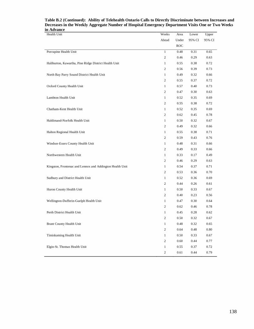
138
Table B.2 (Continued): Ability of Telehealth Ontario Calls to Directly Discriminate between Increases and
Decreases in the Weekly Aggregate Number of Hospital Emergency Department Visits One or Two Weeks
in Advance Health Unit Weeks
Ahead
Area
Under
ROC
Lower
95% CI
Upper
95% CI
Porcupine Health Unit 1 0.48 0.31 0.65
2 0.46 0.29 0.63
Haliburton, Kawartha, Pine Ridge District Health Unit 1 0.55 0.38 0.72
2 0.56 0.39 0.73
North Bay Parry Sound District Health Unit 1 0.49 0.32 0.66
2 0.55 0.37 0.72
Oxford County Health Unit 1 0.57 0.40 0.73
2 0.47 0.30 0.63
Lambton Health Unit 1 0.52 0.35 0.69
2 0.55 0.38 0.72
Chatham-Kent Health Unit 1 0.52 0.35 0.69
2 0.62 0.45 0.78
Haldimand-Norfolk Health Unit 1 0.50 0.32 0.67
2 0.49 0.32 0.66
Halton Regional Health Unit 1 0.55 0.38 0.71
2 0.59 0.43 0.76
Windsor-Essex County Health Unit 1 0.48 0.31 0.66
2 0.49 0.33 0.66
Northwestern Health Unit 1 0.33 0.17 0.49
2 0.46 0.29 0.63
Kingston, Frontenac and Lennox and Addington Health Unit 1 0.54 0.37 0.71
2 0.53 0.36 0.70
Sudbury and District Health Unit 1 0.52 0.36 0.69
2 0.44 0.26 0.61
Huron County Health Unit 1 0.50 0.33 0.67
2 0.40 0.23 0.56
Wellington-Dufferin-Guelph Health Unit 1 0.47 0.30 0.64
2 0.62 0.46 0.78
Perth District Health Unit 1 0.45 0.28 0.62
2 0.50 0.32 0.67
Brant County Health Unit 1 0.48 0.32 0.65
2 0.64 0.48 0.80
Timiskaming Health Unit 1 0.50 0.33 0.67
2 0.60 0.44 0.77
Elgin-St. Thomas Health Unit 1 0.55 0.37 0.72
2 0.61 0.44 0.79

139
Table B.3: Ability to Predict Increases in the Weekly Aggregate Number of Hospital Emergency Department Visits Above a Nominal 10% Increase One
Week Ahead or Nominal 15% Increase Two Weeks Ahead
TP FN TN FP Point
Estimate
Lower
95% CI
Upper
95% CI
Point
Estimate
Lower
95% CI
Upper
95% CI
Point
Estimate
Lower
95% CI
Upper
95% CI
Point
Estimate
Lower
95% CI
Upper
95% CI
City of Toronto Health Unit 1 FOS 2 10 36 0 0.059 1.000 0.36 0.17 0.02 0.48 1.00 0.90 1.00 1.00 0.16 1.00 0.78 0.64 0.89
City of Toronto Health Unit 1.000 PCI 2 10 34 2 0.257 1.000 0.17 0.17 0.02 0.48 0.94 0.81 0.99 0.50 0.07 0.93 0.77 0.62 0.89
City of Toronto Health Unit 1.000 SS 2 10 30 6 1.000 1.000 0.00 0.17 0.02 0.48 0.83 0.67 0.94 0.25 0.03 0.65 0.75 0.59 0.87
City of Toronto Health Unit 2 FOS 2 12 32 2 0.569 1.000 0.14 0.14 0.02 0.43 0.94 0.80 0.99 0.50 0.07 0.93 0.73 0.57 0.85
City of Toronto Health Unit 2.000 PCI 6 8 27 7 0.157 1.000 0.23 0.43 0.18 0.71 0.79 0.62 0.91 0.46 0.19 0.75 0.77 0.60 0.90
City of Toronto Health Unit 2.000 SS 6 8 23 11 0.522 1.000 0.10 0.43 0.18 0.71 0.68 0.49 0.83 0.35 0.14 0.62 0.74 0.55 0.88
Grey Bruce Health Unit 1 FOS 0 8 40 0 1.000 1.000 0.00 0.00 0.37 1.00 0.91 1.00 0.83 0.70 0.93
Grey Bruce Health Unit 1.000 PCI 5 3 32 8 0.025 1.000 0.36 0.63 0.24 0.91 0.80 0.64 0.91 0.38 0.14 0.68 0.91 0.77 0.98
Grey Bruce Health Unit 1.000 SS 2 6 33 7 0.633 1.000 0.07 0.25 0.03 0.65 0.83 0.67 0.93 0.22 0.03 0.60 0.85 0.69 0.94
Grey Bruce Health Unit 2 FOS* 2 10 36 0 0.059 1.000 0.36 0.17 0.02 0.48 1.00 0.90 1.00 1.00 0.16 1.00 0.78 0.64 0.89
Grey Bruce Health Unit 2.000 PCI 6 6 28 8 0.139 1.000 0.26 0.50 0.21 0.79 0.78 0.61 0.90 0.43 0.18 0.71 0.82 0.65 0.93
Grey Bruce Health Unit 2.000 SS 3 9 31 5 0.394 1.000 0.13 0.25 0.05 0.57 0.86 0.71 0.95 0.38 0.09 0.76 0.78 0.62 0.89
Simcoe Muskoka District Health Unit 1 FOS 1 7 37 3 0.530 1.000 0.07 0.13 0.00 0.53 0.93 0.80 0.98 0.25 0.01 0.81 0.84 0.70 0.93
Simcoe Muskoka District Health Uni 1.000 PCI 2 6 37 3 0.189 1.000 0.21 0.25 0.03 0.65 0.93 0.80 0.98 0.40 0.05 0.85 0.86 0.72 0.95
Simcoe Muskoka District Health Uni 1.000 SS 6 2 31 9 0.008 1.000 0.42 0.75 0.35 0.97 0.78 0.62 0.89 0.40 0.16 0.68 0.94 0.80 0.99
Simcoe Muskoka District Health Uni 2 FOS* 0 13 32 3 0.553 1.000 -0.16 0.00 0.00 0.25 0.91 0.77 0.98 0.00 0.00 0.71 0.71 0.56 0.84
Simcoe Muskoka District Health Uni 2.000 PCI 6 7 27 8 0.157 1.000 0.23 0.46 0.19 0.75 0.77 0.60 0.90 0.43 0.18 0.71 0.79 0.62 0.91
Simcoe Muskoka District Health Uni 2.000 SS 6 7 27 8 0.157 1.000 0.23 0.46 0.19 0.75 0.77 0.60 0.90 0.43 0.18 0.71 0.79 0.62 0.91
Niagara Regional Area Health Unit 1 FOS 2 13 32 1 0.227 1.000 0.20 0.13 0.02 0.40 0.97 0.84 1.00 0.67 0.09 0.99 0.71 0.56 0.84
Niagara Regional Area Health Unit 1.000 PCI 3 12 29 4 0.662 1.000 0.10 0.20 0.04 0.48 0.88 0.72 0.97 0.43 0.10 0.82 0.71 0.54 0.84
Niagara Regional Area Health Unit 1.000 SS 6 9 22 11 0.749 1.000 0.06 0.40 0.16 0.68 0.67 0.48 0.82 0.35 0.14 0.62 0.71 0.52 0.86
Niagara Regional Area Health Unit 2 FOS 4 9 33 2 0.038 1.000 0.34 0.31 0.09 0.61 0.94 0.81 0.99 0.67 0.22 0.96 0.79 0.63 0.90
Niagara Regional Area Health Unit 2.000 PCI 5 8 30 5 0.108 1.000 0.26 0.38 0.14 0.68 0.86 0.70 0.95 0.50 0.19 0.81 0.79 0.63 0.90
Niagara Regional Area Health Unit 2.000 SS 5 8 24 11 0.735 1.000 0.07 0.38 0.14 0.68 0.69 0.51 0.83 0.31 0.11 0.59 0.75 0.57 0.89
Peel Regional Health Unit 1 FOS 5 12 25 6 0.486 1.000 0.11 0.29 0.10 0.56 0.81 0.63 0.93 0.45 0.17 0.77 0.68 0.50 0.82
Peel Regional Health Unit 1.000 PCI 4 13 26 5 0.701 1.000 0.09 0.24 0.07 0.50 0.84 0.66 0.95 0.44 0.14 0.79 0.67 0.50 0.81
Peel Regional Health Unit 1.000 SS 4 13 23 8 1.000 1.000 -0.03 0.24 0.07 0.50 0.74 0.55 0.88 0.33 0.10 0.65 0.64 0.46 0.79
Peel Regional Health Unit 2 FOS 7 13 25 3 0.070 1.000 0.29 0.35 0.15 0.59 0.89 0.72 0.98 0.70 0.35 0.93 0.66 0.49 0.80
Peel Regional Health Unit 2.000 PCI 8 12 24 4 0.088 1.000 0.29 0.40 0.19 0.64 0.86 0.67 0.96 0.67 0.35 0.90 0.67 0.49 0.81
Peel Regional Health Unit 2.000 SS 9 11 17 11 0.771 1.000 0.06 0.45 0.23 0.68 0.61 0.41 0.78 0.45 0.23 0.68 0.61 0.41 0.78
City of Ottawa Health Unit 1 FOS 5 9 32 2 0.017 1.000 0.38 0.36 0.13 0.65 0.94 0.80 0.99 0.71 0.29 0.96 0.78 0.62 0.89
City of Ottawa Health Unit 1.000 PCI 5 9 31 3 0.037 1.000 0.33 0.36 0.13 0.65 0.91 0.76 0.98 0.63 0.24 0.91 0.78 0.62 0.89
City of Ottawa Health Unit 1.000 SS 5 9 29 5 0.130 1.000 0.24 0.36 0.13 0.65 0.85 0.69 0.95 0.50 0.19 0.81 0.76 0.60 0.89
City of Ottawa Health Unit 2 FOS 2 14 30 2 0.592 1.000 0.11 0.13 0.02 0.38 0.94 0.79 0.99 0.50 0.07 0.93 0.68 0.52 0.81
City of Ottawa Health Unit 2.000 PCI 6 10 27 5 0.144 1.000 0.25 0.38 0.15 0.65 0.84 0.67 0.95 0.55 0.23 0.83 0.73 0.56 0.86
City of Ottawa Health Unit 2.000 SS 8 8 24 8 0.110 1.000 0.25 0.50 0.25 0.75 0.75 0.57 0.89 0.50 0.25 0.75 0.75 0.57 0.89
Health Unit Weeks
Ahead
Forecasting
Method
Fisher's
Exact Test
p-Value
Specificity Positive Predictive Value Negative Predictive ValueSensitivityConfusion Matrix
for Flagging
Increases
Adjusted p-
Value
Matthew's
Correlation
Coefficient
(MCC)

140
Table B.3 (Continued): Ability to Predict Increases in the Weekly Aggregate Number of Hospital Emergency Department Visits Above a Nominal 10%
Increase One Week Ahead or Nominal 15% Increase Two Weeks Ahead
TP FN TN FP Point
Estimate
Lower
95% CI
Upper
95% CI
Point
Estimate
Lower
95% CI
Upper
95% CI
Point
Estimate
Lower
95% CI
Upper
95% CI
Point
Estimate
Lower
95% CI
Upper
95% CI
City of Hamilton Health Unit 1 FOS 3 7 35 3 0.095 1.000 0.27 0.30 0.07 0.65 0.92 0.79 0.98 0.50 0.12 0.88 0.83 0.69 0.93
City of Hamilton Health Unit 1.000 PCI 2 8 35 3 0.276 1.000 0.16 0.20 0.03 0.56 0.92 0.79 0.98 0.40 0.05 0.85 0.81 0.67 0.92
City of Hamilton Health Unit 1.000 SS 3 7 30 8 0.675 1.000 0.09 0.30 0.07 0.65 0.79 0.63 0.90 0.27 0.06 0.61 0.81 0.65 0.92
City of Hamilton Health Unit 2 FOS 1 14 33 0 0.312 1.000 0.22 0.07 0.00 0.32 1.00 0.89 1.00 1.00 0.03 1.00 0.70 0.55 0.83
City of Hamilton Health Unit 2.000 PCI 3 12 28 5 0.692 1.000 0.06 0.20 0.04 0.48 0.85 0.68 0.95 0.38 0.09 0.76 0.70 0.53 0.83
City of Hamilton Health Unit 2.000 SS 5 10 24 9 0.738 1.000 0.06 0.33 0.12 0.62 0.73 0.54 0.87 0.36 0.13 0.65 0.71 0.53 0.85
York Regional Health Unit 1 FOS 1 14 29 4 1.000 1.000 -0.08 0.07 0.00 0.32 0.88 0.72 0.97 0.20 0.01 0.72 0.67 0.51 0.81
York Regional Health Unit 1.000 PCI 3 12 28 5 0.692 1.000 0.06 0.20 0.04 0.48 0.85 0.68 0.95 0.38 0.09 0.76 0.70 0.53 0.83
York Regional Health Unit 1.000 SS 5 10 27 6 0.283 1.000 0.17 0.33 0.12 0.62 0.82 0.65 0.93 0.45 0.17 0.77 0.73 0.56 0.86
York Regional Health Unit 2 FOS 4 10 30 4 0.208 1.000 0.20 0.29 0.08 0.58 0.88 0.73 0.97 0.50 0.16 0.84 0.75 0.59 0.87
York Regional Health Unit 2.000 PCI 6 8 30 4 0.045 1.000 0.35 0.43 0.18 0.71 0.88 0.73 0.97 0.60 0.26 0.88 0.79 0.63 0.90
York Regional Health Unit 2.000 SS 5 9 25 9 0.728 1.000 0.09 0.36 0.13 0.65 0.74 0.56 0.87 0.36 0.13 0.65 0.74 0.56 0.87
Leeds, Grenville and Lanark District Health Unit1 FOS* 0 9 39 0 1.000 0.00 0.00 0.34 1.00 0.91 1.00 0.81 0.67 0.91
Leeds, Grenville and Lanark Distri 1.000 PCI 4 5 28 11 0.432 1.000 0.14 0.44 0.14 0.79 0.72 0.55 0.85 0.27 0.08 0.55 0.85 0.68 0.95
Leeds, Grenville and Lanark Distri 1.000 SS 5 4 28 11 0.138 1.000 0.23 0.56 0.21 0.86 0.72 0.55 0.85 0.31 0.11 0.59 0.88 0.71 0.96
Leeds, Grenville and Lanark Distri 2 FOS* 0 16 31 1 1.000 1.000 -0.10 0.00 0.00 0.21 0.97 0.84 1.00 0.00 0.00 0.98 0.66 0.51 0.79
Leeds, Grenville and Lanark Distri 2.000 PCI 4 12 21 11 0.742 1.000 -0.10 0.25 0.07 0.52 0.66 0.47 0.81 0.27 0.08 0.55 0.64 0.45 0.80
Leeds, Grenville and Lanark Distri 2.000 SS 7 9 25 7 0.178 1.000 0.23 0.44 0.20 0.70 0.78 0.60 0.91 0.50 0.23 0.77 0.74 0.56 0.87
Middlesex-London Health Unit 1 FOS 4 12 30 2 0.086 1.000 0.27 0.25 0.07 0.52 0.94 0.79 0.99 0.67 0.22 0.96 0.71 0.55 0.84
Middlesex-London Health Unit 1.000 PCI 6 10 26 6 0.178 1.000 0.20 0.38 0.15 0.65 0.81 0.64 0.93 0.50 0.21 0.79 0.72 0.55 0.86
Middlesex-London Health Unit 1.000 SS 4 12 27 5 0.457 1.000 0.11 0.25 0.07 0.52 0.84 0.67 0.95 0.44 0.14 0.79 0.69 0.52 0.83
Middlesex-London Health Unit 2 FOS 5 8 28 7 0.263 1.000 0.19 0.38 0.14 0.68 0.80 0.63 0.92 0.42 0.15 0.72 0.78 0.61 0.90
Middlesex-London Health Unit 2.000 PCI 5 8 27 8 0.298 1.000 0.16 0.38 0.14 0.68 0.77 0.60 0.90 0.38 0.14 0.68 0.77 0.60 0.90
Middlesex-London Health Unit 2.000 SS 4 9 25 10 1.000 1.000 0.02 0.31 0.09 0.61 0.71 0.54 0.85 0.29 0.08 0.58 0.74 0.56 0.87
Durham Regional Health Unit 1 FOS 5 10 32 1 0.008 1.000 0.42 0.33 0.12 0.62 0.97 0.84 1.00 0.83 0.36 1.00 0.76 0.61 0.88
Durham Regional Health Unit 1.000 PCI 5 10 29 4 0.115 1.000 0.25 0.33 0.12 0.62 0.88 0.72 0.97 0.56 0.21 0.86 0.74 0.58 0.87
Durham Regional Health Unit 1.000 SS 5 10 28 5 0.249 1.000 0.21 0.33 0.12 0.62 0.85 0.68 0.95 0.50 0.19 0.81 0.74 0.57 0.87
Durham Regional Health Unit 2 FOS 3 12 31 2 0.307 1.000 0.21 0.20 0.04 0.48 0.94 0.80 0.99 0.60 0.15 0.95 0.72 0.56 0.85
Durham Regional Health Unit 2.000 PCI 4 11 30 3 0.183 1.000 0.23 0.27 0.08 0.55 0.91 0.76 0.98 0.57 0.18 0.90 0.73 0.57 0.86
Durham Regional Health Unit 2.000 SS 5 10 21 12 1.000 1.000 -0.03 0.33 0.12 0.62 0.64 0.45 0.80 0.29 0.10 0.56 0.68 0.49 0.83
The Eastern Ontario Health Unit 1 FOS 1 13 34 0 0.292 1.000 0.23 0.07 0.00 0.34 1.00 0.90 1.00 1.00 0.03 1.00 0.72 0.57 0.84
The Eastern Ontario Health Unit 1.000 PCI 3 11 25 9 1.000 1.000 -0.05 0.21 0.05 0.51 0.74 0.56 0.87 0.25 0.05 0.57 0.69 0.52 0.84
The Eastern Ontario Health Unit 1.000 SS 4 10 25 9 1.000 1.000 0.02 0.29 0.08 0.58 0.74 0.56 0.87 0.31 0.09 0.61 0.71 0.54 0.85
The Eastern Ontario Health Unit 2 FOS 1 13 34 0 0.292 1.000 0.23 0.07 0.00 0.34 1.00 0.90 1.00 1.00 0.03 1.00 0.72 0.57 0.84
The Eastern Ontario Health Unit 2.000 PCI 6 8 28 6 0.139 1.000 0.26 0.43 0.18 0.71 0.82 0.65 0.93 0.50 0.21 0.79 0.78 0.61 0.90
The Eastern Ontario Health Unit 2.000 SS 3 11 26 8 1.000 1.000 -0.02 0.21 0.05 0.51 0.76 0.59 0.89 0.27 0.06 0.61 0.70 0.53 0.84
Positive Predictive Value Negative Predictive ValueHealth Unit Weeks
Ahead
Forecasting
Method
Confusion Matrix Fisher's
Exact Test
p-Value
Adjusted p-
Value
Matthew's
Correlation
Coefficient
(MCC)
Sensitivity Specificity

141
Table B.3 (Continued): Ability to Predict Increases in the Weekly Aggregate Number of Hospital Emergency Department Visits Above a Nominal 10%
Increase One Week Ahead or Nominal 15% Increase Two Weeks Ahead
TP FN TN FP Point
Estimate
Lower
95% CI
Upper
95% CI
Point
Estimate
Lower
95% CI
Upper
95% CI
Point
Estimate
Lower
95% CI
Upper
95% CI
Point
Estimate
Lower
95% CI
Upper
95% CI
Peterborough County-City Health Unit 1 FOS 5 13 27 3 0.132 1.000 0.23 0.28 0.10 0.53 0.90 0.73 0.98 0.63 0.24 0.91 0.68 0.51 0.81
Peterborough County-City Health Un 1.000 PCI 7 11 20 10 0.761 1.000 0.06 0.39 0.17 0.64 0.67 0.47 0.83 0.41 0.18 0.67 0.65 0.45 0.81
Peterborough County-City Health Un 1.000 SS 8 10 21 9 0.361 1.000 0.15 0.44 0.22 0.69 0.70 0.51 0.85 0.47 0.23 0.72 0.68 0.49 0.83
Peterborough County-City Health Un 2 FOS 5 8 28 7 0.263 1.000 0.19 0.38 0.14 0.68 0.80 0.63 0.92 0.42 0.15 0.72 0.78 0.61 0.90
Peterborough County-City Health Un 2.000 PCI 7 6 28 7 0.034 1.000 0.33 0.54 0.25 0.81 0.80 0.63 0.92 0.50 0.23 0.77 0.82 0.65 0.93
Peterborough County-City Health Un 2.000 SS 5 8 22 13 1.000 1.000 0.01 0.38 0.14 0.68 0.63 0.45 0.79 0.28 0.10 0.53 0.73 0.54 0.88
Hastings and Prince Edward Counties Health Unit1 FOS 4 7 37 0 0.002 1.000 0.55 0.36 0.11 0.69 1.00 0.91 1.00 1.00 0.40 1.00 0.84 0.70 0.93
Hastings and Prince Edward Countie 1.000 PCI 6 5 28 9 0.074 1.000 0.27 0.55 0.23 0.83 0.76 0.59 0.88 0.40 0.16 0.68 0.85 0.68 0.95
Hastings and Prince Edward Countie 1.000 SS 6 5 26 11 0.163 1.000 0.22 0.55 0.23 0.83 0.70 0.53 0.84 0.35 0.14 0.62 0.84 0.66 0.95
Hastings and Prince Edward Countie 2 FOS* 2 10 30 6 1.000 1.000 0.00 0.17 0.02 0.48 0.83 0.67 0.94 0.25 0.03 0.65 0.75 0.59 0.87
Hastings and Prince Edward Countie 2.000 PCI 6 6 27 9 0.152 1.000 0.23 0.50 0.21 0.79 0.75 0.58 0.88 0.40 0.16 0.68 0.82 0.65 0.93
Hastings and Prince Edward Countie 2.000 SS 2 10 24 12 0.465 1.000 -0.16 0.17 0.02 0.48 0.67 0.49 0.81 0.14 0.02 0.43 0.71 0.53 0.85
Waterloo Health Unit 1 FOS* 0 17 31 0 1.000 0.00 0.00 0.20 1.00 0.89 1.00 0.65 0.49 0.78
Waterloo Health Unit 1.000 PCI 3 14 26 5 1.000 1.000 0.02 0.18 0.04 0.43 0.84 0.66 0.95 0.38 0.09 0.76 0.65 0.48 0.79
Waterloo Health Unit 1.000 SS 4 13 24 7 1.000 1.000 0.01 0.24 0.07 0.50 0.77 0.59 0.90 0.36 0.11 0.69 0.65 0.47 0.80
Waterloo Health Unit 2 FOS* 14 0 7 27 0.090 1.000 0.27 1.00 0.77 1.00 0.21 0.09 0.38 0.34 0.20 0.51 1.00 0.59 1.00
Waterloo Health Unit 2.000 PCI 6 8 27 7 0.157 1.000 0.23 0.43 0.18 0.71 0.79 0.62 0.91 0.46 0.19 0.75 0.77 0.60 0.90
Waterloo Health Unit 2.000 SS 6 8 24 10 0.503 1.000 0.13 0.43 0.18 0.71 0.71 0.53 0.85 0.38 0.15 0.65 0.75 0.57 0.89
The District of Algoma Health Unit 1 FOS 0 14 33 1 1.000 1.000 -0.09 0.00 0.00 0.23 0.97 0.85 1.00 0.00 0.00 0.98 0.70 0.55 0.83
The District of Algoma Health Unit 1.000 PCI 5 9 23 11 1.000 1.000 0.03 0.36 0.13 0.65 0.68 0.49 0.83 0.31 0.11 0.59 0.72 0.53 0.86
The District of Algoma Health Unit 1.000 SS 6 8 26 8 0.294 1.000 0.19 0.43 0.18 0.71 0.76 0.59 0.89 0.43 0.18 0.71 0.76 0.59 0.89
The District of Algoma Health Unit 2 FOS 3 9 34 2 0.092 1.000 0.28 0.25 0.05 0.57 0.94 0.81 0.99 0.60 0.15 0.95 0.79 0.64 0.90
The District of Algoma Health Unit 2.000 PCI 3 9 19 17 0.311 1.000 -0.20 0.25 0.05 0.57 0.53 0.35 0.70 0.15 0.03 0.38 0.68 0.48 0.84
The District of Algoma Health Unit 2.000 SS 3 9 24 12 0.728 1.000 -0.08 0.25 0.05 0.57 0.67 0.49 0.81 0.20 0.04 0.48 0.73 0.54 0.87
Renfrew County and District Health Unit 1 FOS 1 13 34 0 0.292 1.000 0.23 0.07 0.00 0.34 1.00 0.90 1.00 1.00 0.03 1.00 0.72 0.57 0.84
Renfrew County and District Health 1.000 PCI 4 10 27 7 0.708 1.000 0.09 0.29 0.08 0.58 0.79 0.62 0.91 0.36 0.11 0.69 0.73 0.56 0.86
Renfrew County and District Health 1.000 SS 2 12 25 9 0.469 1.000 -0.13 0.14 0.02 0.43 0.74 0.56 0.87 0.18 0.02 0.52 0.68 0.50 0.82
Renfrew County and District Health 2 FOS 1 15 32 0 0.333 1.000 0.21 0.06 0.00 0.30 1.00 0.89 1.00 1.00 0.03 1.00 0.68 0.53 0.81
Renfrew County and District Health 2.000 PCI 10 6 26 6 0.004 1.000 0.44 0.63 0.35 0.85 0.81 0.64 0.93 0.63 0.35 0.85 0.81 0.64 0.93
Renfrew County and District Health 2.000 SS 3 13 25 7 1.000 1.000 -0.04 0.19 0.04 0.46 0.78 0.60 0.91 0.30 0.07 0.65 0.66 0.49 0.80
Thunder Bay District Health Unit 1 FOS* 5 11 25 7 0.500 1.000 0.10 0.31 0.11 0.59 0.78 0.60 0.91 0.42 0.15 0.72 0.69 0.52 0.84
Thunder Bay District Health Unit 1.000 PCI 5 11 20 12 0.757 1.000 -0.06 0.31 0.11 0.59 0.63 0.44 0.79 0.29 0.10 0.56 0.65 0.45 0.81
Thunder Bay District Health Unit 1.000 SS 4 12 21 11 0.742 1.000 -0.10 0.25 0.07 0.52 0.66 0.47 0.81 0.27 0.08 0.55 0.64 0.45 0.80
Thunder Bay District Health Unit 2 FOS* 13 1 5 29 0.656 1.000 0.10 0.93 0.66 1.00 0.15 0.05 0.31 0.31 0.18 0.47 0.83 0.36 1.00
Thunder Bay District Health Unit 2.000 PCI 6 8 21 13 1.000 1.000 0.04 0.43 0.18 0.71 0.62 0.44 0.78 0.32 0.13 0.57 0.72 0.53 0.87
Thunder Bay District Health Unit 2.000 SS 3 11 23 11 0.510 1.000 -0.11 0.21 0.05 0.51 0.68 0.49 0.83 0.21 0.05 0.51 0.68 0.49 0.83
Specificity Positive Predictive Value Negative Predictive ValueHealth Unit Weeks
Ahead
Forecasting
Method
Confusion Matrix Fisher's
Exact Test
p-Value
Adjusted p-
Value
Matthew's
Correlation
Coefficient
(MCC)
Sensitivity

142
Table B.3 (Continued): Ability to Predict Increases in the Weekly Aggregate Number of Hospital Emergency Department Visits Above a Nominal 10%
Increase One Week Ahead or Nominal 15% Increase Two Weeks Ahead
TP FN TN FP Point
Estimate
Lower
95% CI
Upper
95% CI
Point
Estimate
Lower
95% CI
Upper
95% CI
Point
Estimate
Lower
95% CI
Upper
95% CI
Point
Estimate
Lower
95% CI
Upper
95% CI
Porcupine Health Unit 1 FOS 3 12 30 3 0.360 1.000 0.15 0.20 0.04 0.48 0.91 0.76 0.98 0.50 0.12 0.88 0.71 0.55 0.84
Porcupine Health Unit 1.000 PCI 6 9 25 8 0.315 1.000 0.16 0.40 0.16 0.68 0.76 0.58 0.89 0.43 0.18 0.71 0.74 0.56 0.87
Porcupine Health Unit 1.000 SS 5 10 21 12 1.000 1.000 -0.03 0.33 0.12 0.62 0.64 0.45 0.80 0.29 0.10 0.56 0.68 0.49 0.83
Porcupine Health Unit 2 FOS 2 14 30 2 0.592 1.000 0.11 0.13 0.02 0.38 0.94 0.79 0.99 0.50 0.07 0.93 0.68 0.52 0.81
Porcupine Health Unit 2.000 PCI 7 9 24 8 0.206 1.000 0.19 0.44 0.20 0.70 0.75 0.57 0.89 0.47 0.21 0.73 0.73 0.54 0.87
Porcupine Health Unit 2.000 SS 5 11 20 12 0.757 1.000 -0.06 0.31 0.11 0.59 0.63 0.44 0.79 0.29 0.10 0.56 0.65 0.45 0.81
Haliburton, Kawartha, Pine Ridge District Health Unit1 FOS 2 11 33 2 0.294 1.000 0.16 0.15 0.02 0.45 0.94 0.81 0.99 0.50 0.07 0.93 0.75 0.60 0.87
Haliburton, Kawartha, Pine Ridge D 1.000 PCI 5 8 25 10 0.509 1.000 0.09 0.38 0.14 0.68 0.71 0.54 0.85 0.33 0.12 0.62 0.76 0.58 0.89
Haliburton, Kawartha, Pine Ridge D 1.000 SS 4 9 28 7 0.458 1.000 0.11 0.31 0.09 0.61 0.80 0.63 0.92 0.36 0.11 0.69 0.76 0.59 0.88
Haliburton, Kawartha, Pine Ridge D 2 FOS 4 13 22 9 0.747 1.000 -0.06 0.24 0.07 0.50 0.71 0.52 0.86 0.31 0.09 0.61 0.63 0.45 0.79
Haliburton, Kawartha, Pine Ridge D 2.000 PCI 8 9 25 6 0.055 1.000 0.29 0.47 0.23 0.72 0.81 0.63 0.93 0.57 0.29 0.82 0.74 0.56 0.87
Haliburton, Kawartha, Pine Ridge D 2.000 SS 6 11 23 8 0.522 1.000 0.10 0.35 0.14 0.62 0.74 0.55 0.88 0.43 0.18 0.71 0.68 0.49 0.83
North Bay Parry Sound District Health Unit 1 FOS 1 15 32 0 0.333 1.000 0.21 0.06 0.00 0.30 1.00 0.89 1.00 1.00 0.03 1.00 0.68 0.53 0.81
North Bay Parry Sound District Hea 1.000 PCI 6 10 26 6 0.178 1.000 0.20 0.38 0.15 0.65 0.81 0.64 0.93 0.50 0.21 0.79 0.72 0.55 0.86
North Bay Parry Sound District Hea 1.000 SS 7 9 26 6 0.090 1.000 0.27 0.44 0.20 0.70 0.81 0.64 0.93 0.54 0.25 0.81 0.74 0.57 0.88
North Bay Parry Sound District Hea 2 FOS* 12 4 19 13 0.034 1.000 0.32 0.75 0.48 0.93 0.59 0.41 0.76 0.48 0.28 0.69 0.83 0.61 0.95
North Bay Parry Sound District Hea 2.000 PCI 6 10 26 6 0.178 1.000 0.20 0.38 0.15 0.65 0.81 0.64 0.93 0.50 0.21 0.79 0.72 0.55 0.86
North Bay Parry Sound District Hea 2.000 SS 7 9 23 9 0.339 1.000 0.16 0.44 0.20 0.70 0.72 0.53 0.86 0.44 0.20 0.70 0.72 0.53 0.86
Oxford County Health Unit 1 FOS 1 15 32 0 0.333 1.000 0.21 0.06 0.00 0.30 1.00 0.89 1.00 1.00 0.03 1.00 0.68 0.53 0.81
Oxford County Health Unit 1.000 PCI 4 12 25 7 1.000 1.000 0.04 0.25 0.07 0.52 0.78 0.60 0.91 0.36 0.11 0.69 0.68 0.50 0.82
Oxford County Health Unit 1.000 SS 4 12 27 5 0.457 1.000 0.11 0.25 0.07 0.52 0.84 0.67 0.95 0.44 0.14 0.79 0.69 0.52 0.83
Oxford County Health Unit 2 FOS* 1 13 34 0 0.292 1.000 0.23 0.07 0.00 0.34 1.00 0.90 1.00 1.00 0.03 1.00 0.72 0.57 0.84
Oxford County Health Unit 2.000 PCI 4 10 25 9 1.000 1.000 0.02 0.29 0.08 0.58 0.74 0.56 0.87 0.31 0.09 0.61 0.71 0.54 0.85
Oxford County Health Unit 2.000 SS 6 8 25 9 0.315 1.000 0.16 0.43 0.18 0.71 0.74 0.56 0.87 0.40 0.16 0.68 0.76 0.58 0.89
Lambton Health Unit 1 FOS 4 15 29 0 0.020 1.000 0.37 0.21 0.06 0.46 1.00 0.88 1.00 1.00 0.40 1.00 0.66 0.50 0.80
Lambton Health Unit 1.000 PCI 9 10 22 7 0.124 1.000 0.24 0.47 0.24 0.71 0.76 0.56 0.90 0.56 0.30 0.80 0.69 0.50 0.84
Lambton Health Unit 1.000 SS 5 14 25 4 0.451 1.000 0.16 0.26 0.09 0.51 0.86 0.68 0.96 0.56 0.21 0.86 0.64 0.47 0.79
Lambton Health Unit 2 FOS 2 13 32 1 0.227 1.000 0.20 0.13 0.02 0.40 0.97 0.84 1.00 0.67 0.09 0.99 0.71 0.56 0.84
Lambton Health Unit 2.000 PCI 5 10 23 10 1.000 1.000 0.03 0.33 0.12 0.62 0.70 0.51 0.84 0.33 0.12 0.62 0.70 0.51 0.84
Lambton Health Unit 2.000 SS 5 10 23 10 1.000 1.000 0.03 0.33 0.12 0.62 0.70 0.51 0.84 0.33 0.12 0.62 0.70 0.51 0.84
Chatham-Kent Health Unit 1 FOS 2 15 31 0 0.121 1.000 0.28 0.12 0.01 0.36 1.00 0.89 1.00 1.00 0.16 1.00 0.67 0.52 0.80
Chatham-Kent Health Unit 1.000 PCI 4 13 20 11 0.521 1.000 -0.12 0.24 0.07 0.50 0.65 0.45 0.81 0.27 0.08 0.55 0.61 0.42 0.77
Chatham-Kent Health Unit 1.000 SS 5 12 24 7 0.731 1.000 0.08 0.29 0.10 0.56 0.77 0.59 0.90 0.42 0.15 0.72 0.67 0.49 0.81
Chatham-Kent Health Unit 2 FOS 2 12 29 5 1.000 1.000 -0.01 0.14 0.02 0.43 0.85 0.69 0.95 0.29 0.04 0.71 0.71 0.54 0.84
Chatham-Kent Health Unit 2.000 PCI 5 9 22 12 1.000 1.000 0.00 0.36 0.13 0.65 0.65 0.46 0.80 0.29 0.10 0.56 0.71 0.52 0.86
Chatham-Kent Health Unit 2.000 SS 4 10 27 7 0.708 1.000 0.09 0.29 0.08 0.58 0.79 0.62 0.91 0.36 0.11 0.69 0.73 0.56 0.86
Specificity Positive Predictive Value Negative Predictive ValueFisher's
Exact Test
p-Value
Adjusted p-
Value
Matthew's
Correlation
Coefficient
(MCC)
SensitivityHealth Unit Weeks
Ahead
Forecasting
Method
Confusion Matrix

143
Table B.3 (Continued): Ability to Predict Increases in the Weekly Aggregate Number of Hospital Emergency Department Visits Above a Nominal 10%
Increase One Week Ahead or Nominal 15% Increase Two Weeks Ahead
TP FN TN FP Point
Estimate
Lower
95% CI
Upper
95% CI
Point
Estimate
Lower
95% CI
Upper
95% CI
Point
Estimate
Lower
95% CI
Upper
95% CI
Point
Estimate
Lower
95% CI
Upper
95% CI
Haldimand-Norfolk Health Unit 1 FOS 1 13 27 7 0.407 1.000 -0.16 0.07 0.00 0.34 0.79 0.62 0.91 0.13 0.00 0.53 0.68 0.51 0.81
Haldimand-Norfolk Health Unit 1.000 PCI 3 11 23 11 0.510 1.000 -0.11 0.21 0.05 0.51 0.68 0.49 0.83 0.21 0.05 0.51 0.68 0.49 0.83
Haldimand-Norfolk Health Unit 1.000 SS 4 10 21 13 0.741 1.000 -0.09 0.29 0.08 0.58 0.62 0.44 0.78 0.24 0.07 0.50 0.68 0.49 0.83
Haldimand-Norfolk Health Unit 2 FOS 7 9 27 5 0.073 1.000 0.31 0.44 0.20 0.70 0.84 0.67 0.95 0.58 0.28 0.85 0.75 0.58 0.88
Haldimand-Norfolk Health Unit 2.000 PCI 7 9 20 12 0.759 1.000 0.06 0.44 0.20 0.70 0.63 0.44 0.79 0.37 0.16 0.62 0.69 0.49 0.85
Haldimand-Norfolk Health Unit 2.000 SS 7 9 25 7 0.178 1.000 0.23 0.44 0.20 0.70 0.78 0.60 0.91 0.50 0.23 0.77 0.74 0.56 0.87
Halton Regional Health Unit 1 FOS 5 12 26 5 0.295 1.000 0.16 0.29 0.10 0.56 0.84 0.66 0.95 0.50 0.19 0.81 0.68 0.51 0.82
Halton Regional Health Unit 1.000 PCI 5 12 28 3 0.112 1.000 0.25 0.29 0.10 0.56 0.90 0.74 0.98 0.63 0.24 0.91 0.70 0.53 0.83
Halton Regional Health Unit 1.000 SS 3 14 25 6 1.000 1.000 -0.02 0.18 0.04 0.43 0.81 0.63 0.93 0.33 0.07 0.70 0.64 0.47 0.79
Halton Regional Health Unit 2 FOS 4 12 28 4 0.413 1.000 0.16 0.25 0.07 0.52 0.88 0.71 0.96 0.50 0.16 0.84 0.70 0.53 0.83
Halton Regional Health Unit 2.000 PCI 7 9 25 7 0.178 1.000 0.23 0.44 0.20 0.70 0.78 0.60 0.91 0.50 0.23 0.77 0.74 0.56 0.87
Halton Regional Health Unit 2.000 SS 8 8 22 10 0.226 1.000 0.18 0.50 0.25 0.75 0.69 0.50 0.84 0.44 0.22 0.69 0.73 0.54 0.88
Windsor-Essex County Health Unit 1 FOS 1 11 32 4 1.000 1.000 -0.04 0.08 0.00 0.38 0.89 0.74 0.97 0.20 0.01 0.72 0.74 0.59 0.86
Windsor-Essex County Health Unit 1.000 PCI 3 9 30 6 0.671 1.000 0.09 0.25 0.05 0.57 0.83 0.67 0.94 0.33 0.07 0.70 0.77 0.61 0.89
Windsor-Essex County Health Unit 1.000 SS 5 7 29 7 0.143 1.000 0.22 0.42 0.15 0.72 0.81 0.64 0.92 0.42 0.15 0.72 0.81 0.64 0.92
Windsor-Essex County Health Unit 2 FOS 1 8 37 2 0.472 1.000 0.10 0.11 0.00 0.48 0.95 0.83 0.99 0.33 0.01 0.91 0.82 0.68 0.92
Windsor-Essex County Health Unit 2.000 PCI 1 8 26 13 0.250 1.000 -0.19 0.11 0.00 0.48 0.67 0.50 0.81 0.07 0.00 0.34 0.76 0.59 0.89
Windsor-Essex County Health Unit 2.000 SS 2 7 27 12 1.000 1.000 -0.07 0.22 0.03 0.60 0.69 0.52 0.83 0.14 0.02 0.43 0.79 0.62 0.91
Northwestern Health Unit 1 FOS 1 11 32 4 1.000 1.000 -0.04 0.08 0.00 0.38 0.89 0.74 0.97 0.20 0.01 0.72 0.74 0.59 0.86
Northwestern Health Unit 1.000 PCI 2 10 20 16 0.167 1.000 -0.25 0.17 0.02 0.48 0.56 0.38 0.72 0.11 0.01 0.35 0.67 0.47 0.83
Northwestern Health Unit 1.000 SS 0 12 33 3 0.563 1.000 -0.15 0.00 0.00 0.26 0.92 0.78 0.98 0.00 0.00 0.71 0.73 0.58 0.85
Northwestern Health Unit 2 FOS* 1 20 26 1 1.000 1.000 0.03 0.05 0.00 0.24 0.96 0.81 1.00 0.50 0.01 0.99 0.57 0.41 0.71
Northwestern Health Unit 2.000 PCI 5 16 14 13 0.133 1.000 -0.25 0.24 0.08 0.47 0.52 0.32 0.71 0.28 0.10 0.53 0.47 0.28 0.66
Northwestern Health Unit 2.000 SS 3 18 23 4 1.000 1.000 -0.01 0.14 0.03 0.36 0.85 0.66 0.96 0.43 0.10 0.82 0.56 0.40 0.72
Kingston, Frontenac and Lennox and Addington Health Unit1 FOS 4 11 31 2 0.067 1.000 0.29 0.27 0.08 0.55 0.94 0.80 0.99 0.67 0.22 0.96 0.74 0.58 0.86
Kingston, Frontenac and Lennox and 1.000 PCI 5 10 23 10 1.000 1.000 0.03 0.33 0.12 0.62 0.70 0.51 0.84 0.33 0.12 0.62 0.70 0.51 0.84
Kingston, Frontenac and Lennox and 1.000 SS 6 9 21 12 1.000 1.000 0.03 0.40 0.16 0.68 0.64 0.45 0.80 0.33 0.13 0.59 0.70 0.51 0.85
Kingston, Frontenac and Lennox and 2 FOS 2 15 27 4 1.000 1.000 -0.02 0.12 0.01 0.36 0.87 0.70 0.96 0.33 0.04 0.78 0.64 0.48 0.78
Kingston, Frontenac and Lennox and 2.000 PCI 5 12 19 12 0.753 1.000 -0.09 0.29 0.10 0.56 0.61 0.42 0.78 0.29 0.10 0.56 0.61 0.42 0.78
Kingston, Frontenac and Lennox and 2.000 SS 6 11 17 14 0.555 1.000 -0.10 0.35 0.14 0.62 0.55 0.36 0.73 0.30 0.12 0.54 0.61 0.41 0.78
Sudbury and District Health Unit 1 FOS 2 14 29 3 1.000 1.000 0.05 0.13 0.02 0.38 0.91 0.75 0.98 0.40 0.05 0.85 0.67 0.51 0.81
Sudbury and District Health Unit 1.000 PCI 4 12 24 8 1.000 1.000 0.00 0.25 0.07 0.52 0.75 0.57 0.89 0.33 0.10 0.65 0.67 0.49 0.81
Sudbury and District Health Unit 1.000 SS 6 10 22 10 0.750 1.000 0.06 0.38 0.15 0.65 0.69 0.50 0.84 0.38 0.15 0.65 0.69 0.50 0.84
Sudbury and District Health Unit 2 FOS 0 18 30 0 1.000 0.00 0.00 0.19 1.00 0.88 1.00 0.63 0.47 0.76
Sudbury and District Health Unit 2.000 PCI 10 8 23 7 0.032 1.000 0.33 0.56 0.31 0.78 0.77 0.58 0.90 0.59 0.33 0.82 0.74 0.55 0.88
Sudbury and District Health Unit 2.000 SS 8 10 23 7 0.198 1.000 0.22 0.44 0.22 0.69 0.77 0.58 0.90 0.53 0.27 0.79 0.70 0.51 0.84
Health Unit Weeks
Ahead
Forecasting
Method
Confusion Matrix Fisher's
Exact Test
p-Value
Adjusted p-
Value
Matthew's
Correlation
Coefficient
(MCC)
Sensitivity Specificity Positive Predictive Value Negative Predictive Value

144
Table B.3 (Continued): Ability to Predict Increases in the Weekly Aggregate Number of Hospital Emergency Department Visits Above a Nominal 10%
Increase One Week Ahead or Nominal 15% Increase Two Weeks Ahead
TP FN TN FP Point
Estimate
Lower
95% CI
Upper
95% CI
Point
Estimate
Lower
95% CI
Upper
95% CI
Point
Estimate
Lower
95% CI
Upper
95% CI
Point
Estimate
Lower
95% CI
Upper
95% CI
Huron County Health Unit 1 FOS 4 7 35 2 0.019 1.000 0.39 0.36 0.11 0.69 0.95 0.82 0.99 0.67 0.22 0.96 0.83 0.69 0.93
Huron County Health Unit 1.000 PCI 5 6 26 11 0.468 1.000 0.14 0.45 0.17 0.77 0.70 0.53 0.84 0.31 0.11 0.59 0.81 0.64 0.93
Huron County Health Unit 1.000 SS 6 5 26 11 0.163 1.000 0.22 0.55 0.23 0.83 0.70 0.53 0.84 0.35 0.14 0.62 0.84 0.66 0.95
Huron County Health Unit 2 FOS 3 10 34 1 0.055 1.000 0.33 0.23 0.05 0.54 0.97 0.85 1.00 0.75 0.19 0.99 0.77 0.62 0.89
Huron County Health Unit 2.000 PCI 8 5 24 11 0.096 1.000 0.27 0.62 0.32 0.86 0.69 0.51 0.83 0.42 0.20 0.67 0.83 0.64 0.94
Huron County Health Unit 2.000 SS 6 7 26 9 0.293 1.000 0.20 0.46 0.19 0.75 0.74 0.57 0.88 0.40 0.16 0.68 0.79 0.61 0.91
Wellington-Dufferin-Guelph Health Unit 1 FOS 4 15 27 2 0.197 1.000 0.21 0.21 0.06 0.46 0.93 0.77 0.99 0.67 0.22 0.96 0.64 0.48 0.78
Wellington-Dufferin-Guelph Health 1.000 PCI 6 13 21 8 1.000 1.000 0.04 0.32 0.13 0.57 0.72 0.53 0.87 0.43 0.18 0.71 0.62 0.44 0.78
Wellington-Dufferin-Guelph Health 1.000 SS 5 14 23 6 0.732 1.000 0.07 0.26 0.09 0.51 0.79 0.60 0.92 0.45 0.17 0.77 0.62 0.45 0.78
Wellington-Dufferin-Guelph Health 2 FOS 5 13 27 3 0.132 1.000 0.23 0.28 0.10 0.53 0.90 0.73 0.98 0.63 0.24 0.91 0.68 0.51 0.81
Wellington-Dufferin-Guelph Health 2.000 PCI 8 10 22 8 0.226 1.000 0.18 0.44 0.22 0.69 0.73 0.54 0.88 0.50 0.25 0.75 0.69 0.50 0.84
Wellington-Dufferin-Guelph Health 2.000 SS 8 10 24 6 0.103 1.000 0.26 0.44 0.22 0.69 0.80 0.61 0.92 0.57 0.29 0.82 0.71 0.53 0.85
Perth District Health Unit 1 FOS 2 17 22 7 0.286 1.000 -0.17 0.11 0.01 0.33 0.76 0.56 0.90 0.22 0.03 0.60 0.56 0.40 0.72
Perth District Health Unit 1.000 PCI 6 13 21 8 1.000 1.000 0.04 0.32 0.13 0.57 0.72 0.53 0.87 0.43 0.18 0.71 0.62 0.44 0.78
Perth District Health Unit 1.000 SS 8 11 15 14 0.771 1.000 -0.06 0.42 0.20 0.67 0.52 0.33 0.71 0.36 0.17 0.59 0.58 0.37 0.77
Perth District Health Unit 2 FOS 2 15 29 2 0.607 1.000 0.09 0.12 0.01 0.36 0.94 0.79 0.99 0.50 0.07 0.93 0.66 0.50 0.80
Perth District Health Unit 2.000 PCI 3 14 20 11 0.320 1.000 -0.19 0.18 0.04 0.43 0.65 0.45 0.81 0.21 0.05 0.51 0.59 0.41 0.75
Perth District Health Unit 2.000 SS 5 12 18 13 0.536 1.000 -0.12 0.29 0.10 0.56 0.58 0.39 0.75 0.28 0.10 0.53 0.60 0.41 0.77
Brant County Health Unit 1 FOS 3 14 27 4 0.686 1.000 0.06 0.18 0.04 0.43 0.87 0.70 0.96 0.43 0.10 0.82 0.66 0.49 0.80
Brant County Health Unit 1.000 PCI 5 12 24 7 0.731 1.000 0.08 0.29 0.10 0.56 0.77 0.59 0.90 0.42 0.15 0.72 0.67 0.49 0.81
Brant County Health Unit 1.000 SS 7 10 26 5 0.083 1.000 0.28 0.41 0.18 0.67 0.84 0.66 0.95 0.58 0.28 0.85 0.72 0.55 0.86
Brant County Health Unit 2 FOS 0 14 30 4 0.307 1.000 -0.19 0.00 0.00 0.23 0.88 0.73 0.97 0.00 0.00 0.60 0.68 0.52 0.81
Brant County Health Unit 2.000 PCI 6 8 25 9 0.315 1.000 0.16 0.43 0.18 0.71 0.74 0.56 0.87 0.40 0.16 0.68 0.76 0.58 0.89
Brant County Health Unit 2.000 SS 4 10 25 9 1.000 1.000 0.02 0.29 0.08 0.58 0.74 0.56 0.87 0.31 0.09 0.61 0.71 0.54 0.85
Timiskaming Health Unit 1 FOS 5 10 31 2 0.024 1.000 0.36 0.33 0.12 0.62 0.94 0.80 0.99 0.71 0.29 0.96 0.76 0.60 0.88
Timiskaming Health Unit 1.000 PCI 4 11 21 12 0.742 1.000 -0.10 0.27 0.08 0.55 0.64 0.45 0.80 0.25 0.07 0.52 0.66 0.47 0.81
Timiskaming Health Unit 1.000 SS 6 9 23 10 0.527 1.000 0.10 0.40 0.16 0.68 0.70 0.51 0.84 0.38 0.15 0.65 0.72 0.53 0.86
Timiskaming Health Unit 2 FOS 2 15 27 4 1.000 1.000 -0.02 0.12 0.01 0.36 0.87 0.70 0.96 0.33 0.04 0.78 0.64 0.48 0.78
Timiskaming Health Unit 2.000 PCI 7 10 20 11 0.761 1.000 0.06 0.41 0.18 0.67 0.65 0.45 0.81 0.39 0.17 0.64 0.67 0.47 0.83
Timiskaming Health Unit 2.000 SS 5 12 23 8 1.000 1.000 0.04 0.29 0.10 0.56 0.74 0.55 0.88 0.38 0.14 0.68 0.66 0.48 0.81
Elgin-St. Thomas Health Unit 1 FOS 2 18 24 4 1.000 1.000 -0.06 0.10 0.01 0.32 0.86 0.67 0.96 0.33 0.04 0.78 0.57 0.41 0.72
Elgin-St. Thomas Health Unit 1.000 PCI 10 10 18 10 0.382 1.000 0.14 0.50 0.27 0.73 0.64 0.44 0.81 0.50 0.27 0.73 0.64 0.44 0.81
Elgin-St. Thomas Health Unit 1.000 SS 7 13 18 10 1.000 1.000 -0.01 0.35 0.15 0.59 0.64 0.44 0.81 0.41 0.18 0.67 0.58 0.39 0.75
Elgin-St. Thomas Health Unit 2 FOS 1 18 28 1 1.000 1.000 0.04 0.05 0.00 0.26 0.97 0.82 1.00 0.50 0.01 0.99 0.61 0.45 0.75
Elgin-St. Thomas Health Unit 2.000 PCI 8 11 20 9 0.541 1.000 0.11 0.42 0.20 0.67 0.69 0.49 0.85 0.47 0.23 0.72 0.65 0.45 0.81
Elgin-St. Thomas Health Unit 2.000 SS 8 11 18 11 1.000 1.000 0.04 0.42 0.20 0.67 0.62 0.42 0.79 0.42 0.20 0.67 0.62 0.42 0.79
Positive Predictive Value Negative Predictive ValueAdjusted p-
Value
Matthew's
Correlation
Coefficient
(MCC)
Sensitivity SpecificityHealth Unit Weeks
Ahead
Forecasting
Method
Confusion Matrix Fisher's
Exact Test
p-Value

145
Table B.4: Ability of Telehealth Ontario Calls to Directly Predict Increases the Weekly Aggregate
Number of Hospital Emergency Department Visits Above a Nominal 10% Increase One Week Ahead
or Nominal 15% Increase Two Weeks Ahead Health Unit Weeks
Ahead
Area
Under
ROC
Lower
95% CI
Upper
95% CI
City of Toronto Health Unit 1 0.70 0.55 0.86
2 0.67 0.52 0.83
Grey Bruce Health Unit 1 0.74 0.57 0.91
2 0.62 0.43 0.80
Simcoe Muskoka District Health Unit 1 0.63 0.39 0.88
2 0.52 0.31 0.73
Niagara Regional Area Health Unit 1 0.52 0.34 0.70
2 0.65 0.49 0.81
Peel Regional Health Unit 1 0.50 0.33 0.67
2 0.68 0.52 0.83
City of Ottawa Health Unit 1 0.66 0.46 0.86
2 0.69 0.51 0.87
City of Hamilton Health Unit 1 0.68 0.49 0.86
2 0.55 0.37 0.72
York Regional Health Unit 1 0.57 0.41 0.74
2 0.61 0.45 0.78
Leeds, Grenville and Lanark District Health Unit 1 0.64 0.47 0.81
2 0.57 0.40 0.74
Middlesex-London Health Unit 1 0.69 0.53 0.84
2 0.61 0.43 0.79
Durham Regional Health Unit 1 0.69 0.54 0.85
2 0.59 0.40 0.77
The Eastern Ontario Health Unit 1 0.42 0.23 0.61
2 0.51 0.31 0.70
Peterborough County-City Health Unit 1 0.56 0.39 0.73
2 0.56 0.39 0.72
Hastings and Prince Edward Counties Health Unit 1 0.60 0.39 0.81
2 0.56 0.36 0.75
Waterloo Health Unit 1 0.53 0.36 0.70
2 0.63 0.47 0.79
The District of Algoma Health Unit 1 0.55 0.33 0.76
2 0.56 0.35 0.77
Renfrew County and District Health Unit 1 0.55 0.36 0.75
2 0.44 0.25 0.63
Thunder Bay District Health Unit 1 0.47 0.29 0.64
2 0.57 0.40 0.74

146
Table B.4 (Continued): Ability of Telehealth Ontario Calls to Directly Predict Increases the Weekly
Aggregate Number of Hospital Emergency Department Visits Above a Nominal 10% Increase One
Week Ahead or Nominal 15% Increase Two Weeks Ahead Health Unit Weeks
Ahead
Area
Under
ROC
Lower
95% CI
Upper
95% CI
Porcupine Health Unit 1 0.52 0.32 0.72
2 0.51 0.33 0.69
Haliburton, Kawartha, Pine Ridge District Health Unit 1 0.65 0.46 0.84
2 0.58 0.41 0.75
North Bay Parry Sound District Health Unit 1 0.65 0.48 0.82
2 0.57 0.40 0.75
Oxford County Health Unit 1 0.43 0.25 0.61
2 0.52 0.32 0.72
Lambton Health Unit 1 0.53 0.35 0.70
2 0.49 0.31 0.66
Chatham-Kent Health Unit 1 0.62 0.46 0.78
2 0.57 0.39 0.75
Haldimand-Norfolk Health Unit 1 0.43 0.24 0.63
2 0.55 0.37 0.72
Halton Regional Health Unit 1 0.48 0.29 0.66
2 0.66 0.49 0.84
Windsor-Essex County Health Unit 1 0.61 0.41 0.80
2 0.59 0.41 0.77
Northwestern Health Unit 1 0.41 0.24 0.58
2 0.39 0.22 0.56
Kingston, Frontenac and Lennox and Addington Health Unit 1 0.59 0.41 0.77
2 0.50 0.31 0.69
Sudbury and District Health Unit 1 0.54 0.37 0.72
2 0.54 0.37 0.72
Huron County Health Unit 1 0.62 0.42 0.81
2 0.54 0.35 0.73
Wellington-Dufferin-Guelph Health Unit 1 0.53 0.37 0.70
2 0.58 0.41 0.75
Perth District Health Unit 1 0.61 0.44 0.78
2 0.58 0.40 0.76
Brant County Health Unit 1 0.61 0.44 0.78
2 0.65 0.49 0.81
Timiskaming Health Unit 1 0.44 0.27 0.62
2 0.57 0.40 0.74
Elgin-St. Thomas Health Unit 1 0.62 0.45 0.78
2 0.64 0.48 0.79

147
Table B.5: Ability to Discriminate Between Increases and Decreases in the Aggregate Number of Hospital Emergency Department Visits over the Next
Four-Days
TP FN TN FP Point
Estimate
Lower
95% CI
Upper
95% CI
Point
Estimate
Lower
95% CI
Upper
95% CI
Point
Estimate
Lower
95% CI
Upper
95% CI
Point
Estimate
Lower
95% CI
Upper
95% CI
City of Toronto Health Unit FOS 40 7 35 7 0.000 0.000 0.68 0.85 0.72 0.94 0.83 0.69 0.93 0.85 0.72 0.94 0.83 0.69 0.93
City of Toronto Health Unit PCI 39 8 35 7 0.000 0.000 0.66 0.83 0.69 0.92 0.83 0.69 0.93 0.85 0.71 0.94 0.81 0.67 0.92
City of Toronto Health Unit SS 37 10 33 9 0.000 0.000 0.57 0.79 0.64 0.89 0.79 0.63 0.90 0.80 0.66 0.91 0.77 0.61 0.88
Grey Bruce Health Unit FOS 23 18 32 16 0.035 1.000 0.23 0.56 0.40 0.72 0.67 0.52 0.80 0.59 0.42 0.74 0.64 0.49 0.77
Grey Bruce Health Unit PCI 27 14 28 20 0.033 1.000 0.24 0.66 0.49 0.80 0.58 0.43 0.72 0.57 0.42 0.72 0.67 0.50 0.80
Grey Bruce Health Unit SS 25 16 29 19 0.057 1.000 0.21 0.61 0.45 0.76 0.60 0.45 0.74 0.57 0.41 0.72 0.64 0.49 0.78
Simcoe Muskoka District Health Unit FOS 21 24 24 20 1.000 1.000 0.01 0.47 0.32 0.62 0.55 0.39 0.70 0.51 0.35 0.67 0.50 0.35 0.65
Simcoe Muskoka District Health Uni PCI 23 22 23 21 0.833 1.000 0.03 0.51 0.36 0.66 0.52 0.37 0.68 0.52 0.37 0.68 0.51 0.36 0.66
Simcoe Muskoka District Health Uni SS 23 22 22 22 1.000 1.000 0.01 0.51 0.36 0.66 0.50 0.35 0.65 0.51 0.36 0.66 0.50 0.35 0.65
Niagara Regional Area Health Unit FOS 26 14 33 16 0.003 0.319 0.32 0.65 0.48 0.79 0.67 0.52 0.80 0.62 0.46 0.76 0.70 0.55 0.83
Niagara Regional Area Health Unit PCI 28 12 29 20 0.010 1.000 0.29 0.70 0.53 0.83 0.59 0.44 0.73 0.58 0.43 0.72 0.71 0.54 0.84
Niagara Regional Area Health Unit SS 19 21 26 23 1.000 1.000 0.01 0.48 0.32 0.64 0.53 0.38 0.67 0.45 0.30 0.61 0.55 0.40 0.70
Peel Regional Health Unit FOS 32 12 34 11 0.000 0.001 0.48 0.73 0.57 0.85 0.76 0.60 0.87 0.74 0.59 0.86 0.74 0.59 0.86
Peel Regional Health Unit PCI 34 10 32 13 0.000 0.001 0.48 0.77 0.62 0.89 0.71 0.56 0.84 0.72 0.57 0.84 0.76 0.61 0.88
Peel Regional Health Unit SS 32 12 32 13 0.000 0.005 0.44 0.73 0.57 0.85 0.71 0.56 0.84 0.71 0.56 0.84 0.73 0.57 0.85
City of Ottawa Health Unit FOS 27 14 32 16 0.003 0.316 0.32 0.66 0.49 0.80 0.67 0.52 0.80 0.63 0.47 0.77 0.70 0.54 0.82
City of Ottawa Health Unit PCI 27 14 29 19 0.019 1.000 0.26 0.66 0.49 0.80 0.60 0.45 0.74 0.59 0.43 0.73 0.67 0.51 0.81
City of Ottawa Health Unit SS 23 18 28 20 0.205 1.000 0.14 0.56 0.40 0.72 0.58 0.43 0.72 0.53 0.38 0.69 0.61 0.45 0.75
City of Hamilton Health Unit FOS 25 17 30 17 0.035 1.000 0.23 0.60 0.43 0.74 0.64 0.49 0.77 0.60 0.43 0.74 0.64 0.49 0.77
City of Hamilton Health Unit PCI 26 16 28 19 0.057 1.000 0.21 0.62 0.46 0.76 0.60 0.44 0.74 0.58 0.42 0.72 0.64 0.48 0.78
City of Hamilton Health Unit SS 26 16 31 16 0.011 1.000 0.28 0.62 0.46 0.76 0.66 0.51 0.79 0.62 0.46 0.76 0.66 0.51 0.79
York Regional Health Unit FOS 34 9 36 10 0.000 0.000 0.57 0.79 0.64 0.90 0.78 0.64 0.89 0.77 0.62 0.89 0.80 0.65 0.90
York Regional Health Unit PCI 35 8 36 10 0.000 0.000 0.60 0.81 0.67 0.92 0.78 0.64 0.89 0.78 0.63 0.89 0.82 0.67 0.92
York Regional Health Unit SS 36 7 35 11 0.000 0.000 0.60 0.84 0.69 0.93 0.76 0.61 0.87 0.77 0.62 0.88 0.83 0.69 0.93
FOS 22 25 25 17 0.669 1.000 0.06 0.47 0.32 0.62 0.60 0.43 0.74 0.56 0.40 0.72 0.50 0.36 0.64
PCI 25 22 21 21 0.833 1.000 0.03 0.53 0.38 0.68 0.50 0.34 0.66 0.54 0.39 0.69 0.49 0.33 0.65
Leeds, Grenville and Lanark Distri SS 21 26 25 17 0.830 1.000 0.04 0.45 0.30 0.60 0.60 0.43 0.74 0.55 0.38 0.71 0.49 0.35 0.63
Middlesex-London Health Unit FOS 30 18 25 16 0.034 1.000 0.23 0.63 0.47 0.76 0.61 0.45 0.76 0.65 0.50 0.79 0.58 0.42 0.73
Middlesex-London Health Unit PCI 27 21 26 15 0.088 1.000 0.20 0.56 0.41 0.71 0.63 0.47 0.78 0.64 0.48 0.78 0.55 0.40 0.70
Middlesex-London Health Unit SS 31 17 25 16 0.020 1.000 0.26 0.65 0.49 0.78 0.61 0.45 0.76 0.66 0.51 0.79 0.60 0.43 0.74
Durham Regional Health Unit FOS 30 13 34 12 0.000 0.005 0.44 0.70 0.54 0.83 0.74 0.59 0.86 0.71 0.55 0.84 0.72 0.57 0.84
Durham Regional Health Unit PCI 32 11 33 13 0.000 0.002 0.46 0.74 0.59 0.86 0.72 0.57 0.84 0.71 0.56 0.84 0.75 0.60 0.87
Durham Regional Health Unit SS 30 13 31 15 0.001 0.070 0.37 0.70 0.54 0.83 0.67 0.52 0.80 0.67 0.51 0.80 0.70 0.55 0.83
The Eastern Ontario Health Unit FOS 28 18 29 14 0.011 1.000 0.28 0.61 0.45 0.75 0.67 0.51 0.81 0.67 0.50 0.80 0.62 0.46 0.75
The Eastern Ontario Health Unit PCI 28 18 31 12 0.003 0.291 0.33 0.61 0.45 0.75 0.72 0.56 0.85 0.70 0.53 0.83 0.63 0.48 0.77
The Eastern Ontario Health Unit SS 28 18 27 16 0.034 1.000 0.24 0.61 0.45 0.75 0.63 0.47 0.77 0.64 0.48 0.78 0.60 0.44 0.74
Leeds, Grenville and Lanark District
Health Unit
Health Unit Forecasting
Method
Fisher's
Exact Test
p-Value
Specificity Positive Predictive Value Negative Predictive ValueSensitivityConfusion Matrix
for Flagging
Increases
Adjusted p-
Value
Matthew's
Correlation
Coefficient
(MCC)

148
Table B.5 (Continued): Ability to Discriminate Between Increases and Decreases in the Aggregate Number of Hospital Emergency Department Visits
over the Next Four-Days
TP FN TN FP Point
Estimate
Lower
95% CI
Upper
95% CI
Point
Estimate
Lower
95% CI
Upper
95% CI
Point
Estimate
Lower
95% CI
Upper
95% CI
Point
Estimate
Lower
95% CI
Upper
95% CI
Peterborough County-City Health Unit FOS 26 17 26 20 0.139 1.000 0.17 0.60 0.44 0.75 0.57 0.41 0.71 0.57 0.41 0.71 0.60 0.44 0.75
Peterborough County-City Health Un PCI 21 22 23 23 1.000 1.000 -0.01 0.49 0.33 0.65 0.50 0.35 0.65 0.48 0.32 0.63 0.51 0.36 0.66
Peterborough County-City Health Un SS 25 18 24 22 0.397 1.000 0.10 0.58 0.42 0.73 0.52 0.37 0.67 0.53 0.38 0.68 0.57 0.41 0.72
FOS 20 22 18 29 0.206 1.000 -0.14 0.48 0.32 0.64 0.38 0.25 0.54 0.41 0.27 0.56 0.45 0.29 0.62
PCI 22 20 25 22 0.673 1.000 0.06 0.52 0.36 0.68 0.53 0.38 0.68 0.50 0.35 0.65 0.56 0.40 0.70
Hastings and Prince Edward Countie SS 22 20 21 26 0.833 1.000 -0.03 0.52 0.36 0.68 0.45 0.30 0.60 0.46 0.31 0.61 0.51 0.35 0.67
Waterloo Health Unit FOS 33 14 31 11 0.000 0.005 0.44 0.70 0.55 0.83 0.74 0.58 0.86 0.75 0.60 0.87 0.69 0.53 0.82
Waterloo Health Unit PCI 28 19 24 18 0.140 1.000 0.17 0.60 0.44 0.74 0.57 0.41 0.72 0.61 0.45 0.75 0.56 0.40 0.71
Waterloo Health Unit SS 26 21 27 15 0.088 1.000 0.20 0.55 0.40 0.70 0.64 0.48 0.78 0.63 0.47 0.78 0.56 0.41 0.71
The District of Algoma Health Unit FOS 17 25 29 18 1.000 1.000 0.02 0.40 0.26 0.57 0.62 0.46 0.75 0.49 0.31 0.66 0.54 0.40 0.67
The District of Algoma Health Unit PCI 21 21 19 28 0.399 1.000 -0.10 0.50 0.34 0.66 0.40 0.26 0.56 0.43 0.29 0.58 0.48 0.32 0.64
The District of Algoma Health Unit SS 21 21 25 22 0.833 1.000 0.03 0.50 0.34 0.66 0.53 0.38 0.68 0.49 0.33 0.65 0.54 0.39 0.69
FOS 31 13 32 13 0.000 0.013 0.42 0.70 0.55 0.83 0.71 0.56 0.84 0.70 0.55 0.83 0.71 0.56 0.84
PCI 25 19 27 18 0.140 1.000 0.17 0.57 0.41 0.72 0.60 0.44 0.74 0.58 0.42 0.73 0.59 0.43 0.73
Renfrew County and District Health SS 26 18 22 23 0.525 1.000 0.08 0.59 0.43 0.74 0.49 0.34 0.64 0.53 0.38 0.67 0.55 0.38 0.71
Thunder Bay District Health Unit FOS* 25 14 30 20 0.033 1.000 0.24 0.64 0.47 0.79 0.60 0.45 0.74 0.56 0.40 0.70 0.68 0.52 0.81
Thunder Bay District Health Unit PCI 24 15 32 18 0.020 1.000 0.25 0.62 0.45 0.77 0.64 0.49 0.77 0.57 0.41 0.72 0.68 0.53 0.81
Thunder Bay District Health Unit SS 21 18 26 24 0.671 1.000 0.06 0.54 0.37 0.70 0.52 0.37 0.66 0.47 0.32 0.62 0.59 0.43 0.74
Porcupine Health Unit FOS 18 22 30 19 0.666 1.000 0.06 0.45 0.29 0.62 0.61 0.46 0.75 0.49 0.32 0.66 0.58 0.43 0.71
Porcupine Health Unit PCI 21 19 27 22 0.527 1.000 0.08 0.53 0.36 0.68 0.55 0.40 0.69 0.49 0.33 0.65 0.59 0.43 0.73
Porcupine Health Unit SS 20 20 27 22 0.674 1.000 0.05 0.50 0.34 0.66 0.55 0.40 0.69 0.48 0.32 0.64 0.57 0.42 0.72
FOS 27 23 24 15 0.199 1.000 0.15 0.54 0.39 0.68 0.62 0.45 0.77 0.64 0.48 0.78 0.51 0.36 0.66
PCI 32 18 23 16 0.035 1.000 0.23 0.64 0.49 0.77 0.59 0.42 0.74 0.67 0.52 0.80 0.56 0.40 0.72
Haliburton, Kawartha, Pine Ridge D SS 28 22 19 20 0.675 1.000 0.05 0.56 0.41 0.70 0.49 0.32 0.65 0.58 0.43 0.72 0.46 0.31 0.63
FOS 26 19 26 18 0.140 1.000 0.17 0.58 0.42 0.72 0.59 0.43 0.74 0.59 0.43 0.74 0.58 0.42 0.72
PCI 23 22 21 23 1.000 1.000 -0.01 0.51 0.36 0.66 0.48 0.32 0.63 0.50 0.35 0.65 0.49 0.33 0.65
North Bay Parry Sound District Hea SS 21 24 25 19 0.832 1.000 0.04 0.47 0.32 0.62 0.57 0.41 0.72 0.53 0.36 0.68 0.51 0.36 0.66
Oxford County Health Unit FOS 28 13 30 18 0.006 0.596 0.31 0.68 0.52 0.82 0.63 0.47 0.76 0.61 0.45 0.75 0.70 0.54 0.83
Oxford County Health Unit PCI 25 16 25 23 0.287 1.000 0.13 0.61 0.45 0.76 0.52 0.37 0.67 0.52 0.37 0.67 0.61 0.45 0.76
Oxford County Health Unit SS 28 13 31 17 0.003 0.305 0.33 0.68 0.52 0.82 0.65 0.49 0.78 0.62 0.47 0.76 0.70 0.55 0.83
Lambton Health Unit FOS 26 23 27 13 0.058 1.000 0.21 0.53 0.38 0.67 0.68 0.51 0.81 0.67 0.50 0.81 0.54 0.39 0.68
Lambton Health Unit PCI 31 18 22 18 0.093 1.000 0.18 0.63 0.48 0.77 0.55 0.38 0.71 0.63 0.48 0.77 0.55 0.38 0.71
Lambton Health Unit SS 27 22 23 17 0.289 1.000 0.13 0.55 0.40 0.69 0.58 0.41 0.73 0.61 0.45 0.76 0.51 0.36 0.66
Chatham-Kent Health Unit FOS 21 21 31 16 0.139 1.000 0.16 0.50 0.34 0.66 0.66 0.51 0.79 0.57 0.39 0.73 0.60 0.45 0.73
Chatham-Kent Health Unit PCI 20 22 20 27 0.399 1.000 -0.10 0.48 0.32 0.64 0.43 0.28 0.58 0.43 0.28 0.58 0.48 0.32 0.64
Chatham-Kent Health Unit SS 21 21 26 21 0.674 1.000 0.05 0.50 0.34 0.66 0.55 0.40 0.70 0.50 0.34 0.66 0.55 0.40 0.70
Hastings and Prince Edward Counties
Health Unit
Renfrew County and District Health
Unit
Haliburton, Kawartha, Pine Ridge
District Health Unit
North Bay Parry Sound District Health
Unit
Positive Predictive Value Negative Predictive ValueHealth Unit Forecasting
Method
Confusion Matrix
for Flagging
Increases
Fisher's
Exact Test
p-Value
Adjusted p-
Value
Matthew's
Correlation
Coefficient
(MCC)
Sensitivity Specificity

149
Table B.5 (Continued): Ability to Discriminate Between Increases and Decreases in the Aggregate Number of Hospital Emergency Department Visits
over the Next Four-Days
TP FN TN FP Point
Estimate
Lower
95% CI
Upper
95% CI
Point
Estimate
Lower
95% CI
Upper
95% CI
Point
Estimate
Lower
95% CI
Upper
95% CI
Point
Estimate
Lower
95% CI
Upper
95% CI
Haldimand-Norfolk Health Unit FOS 20 18 22 29 0.830 1.000 -0.04 0.53 0.36 0.69 0.43 0.29 0.58 0.41 0.27 0.56 0.55 0.38 0.71
Haldimand-Norfolk Health Unit PCI 26 12 26 25 0.085 1.000 0.19 0.68 0.51 0.82 0.51 0.37 0.65 0.51 0.37 0.65 0.68 0.51 0.82
Haldimand-Norfolk Health Unit SS 19 19 26 25 1.000 1.000 0.01 0.50 0.33 0.67 0.51 0.37 0.65 0.43 0.28 0.59 0.58 0.42 0.72
Halton Regional Health Unit FOS 31 8 36 14 0.000 0.000 0.51 0.79 0.64 0.91 0.72 0.58 0.84 0.69 0.53 0.82 0.82 0.67 0.92
Halton Regional Health Unit PCI 29 10 35 15 0.000 0.005 0.44 0.74 0.58 0.87 0.70 0.55 0.82 0.66 0.50 0.80 0.78 0.63 0.89
Halton Regional Health Unit SS 28 11 34 16 0.000 0.028 0.39 0.72 0.55 0.85 0.68 0.53 0.80 0.64 0.48 0.78 0.76 0.60 0.87
Windsor-Essex County Health Unit FOS 33 10 34 12 0.000 0.000 0.51 0.77 0.61 0.88 0.74 0.59 0.86 0.73 0.58 0.85 0.77 0.62 0.89
Windsor-Essex County Health Unit PCI 34 9 33 13 0.000 0.000 0.51 0.79 0.64 0.90 0.72 0.57 0.84 0.72 0.57 0.84 0.79 0.63 0.90
Windsor-Essex County Health Unit SS 31 12 33 13 0.000 0.005 0.44 0.72 0.56 0.85 0.72 0.57 0.84 0.70 0.55 0.83 0.73 0.58 0.85
Northwestern Health Unit FOS* 24 17 24 24 0.523 1.000 0.09 0.59 0.42 0.74 0.50 0.35 0.65 0.50 0.35 0.65 0.59 0.42 0.74
Northwestern Health Unit PCI 21 20 19 29 0.401 1.000 -0.09 0.51 0.35 0.67 0.40 0.26 0.55 0.42 0.28 0.57 0.49 0.32 0.65
Northwestern Health Unit SS 19 22 23 25 0.672 1.000 -0.06 0.46 0.31 0.63 0.48 0.33 0.63 0.43 0.28 0.59 0.51 0.36 0.66
FOS 26 17 29 17 0.034 1.000 0.24 0.60 0.44 0.75 0.63 0.48 0.77 0.60 0.44 0.75 0.63 0.48 0.77
PCI 24 19 26 20 0.292 1.000 0.12 0.56 0.40 0.71 0.57 0.41 0.71 0.55 0.39 0.70 0.58 0.42 0.72
Kingston, Frontenac and Lennox and SS 23 20 26 20 0.399 1.000 0.10 0.53 0.38 0.69 0.57 0.41 0.71 0.53 0.38 0.69 0.57 0.41 0.71
Sudbury and District Health Unit FOS 25 21 24 19 0.399 1.000 0.10 0.54 0.39 0.69 0.56 0.40 0.71 0.57 0.41 0.72 0.53 0.38 0.68
Sudbury and District Health Unit PCI 27 19 24 19 0.206 1.000 0.15 0.59 0.43 0.73 0.56 0.40 0.71 0.59 0.43 0.73 0.56 0.40 0.71
Sudbury and District Health Unit SS 19 27 18 25 0.140 1.000 -0.17 0.41 0.27 0.57 0.42 0.27 0.58 0.43 0.28 0.59 0.40 0.26 0.56
Huron County Health Unit FOS 24 20 27 18 0.205 1.000 0.15 0.55 0.39 0.70 0.60 0.44 0.74 0.57 0.41 0.72 0.57 0.42 0.72
Huron County Health Unit PCI 24 20 20 25 1.000 1.000 -0.01 0.55 0.39 0.70 0.44 0.30 0.60 0.49 0.34 0.64 0.50 0.34 0.66
Huron County Health Unit SS 23 21 26 19 0.399 1.000 0.10 0.52 0.37 0.68 0.58 0.42 0.72 0.55 0.39 0.70 0.55 0.40 0.70
Wellington-Dufferin-Guelph Health Unit FOS 24 20 26 19 0.292 1.000 0.12 0.55 0.39 0.70 0.58 0.42 0.72 0.56 0.40 0.71 0.57 0.41 0.71
Wellington-Dufferin-Guelph Health PCI 23 21 26 19 0.399 1.000 0.10 0.52 0.37 0.68 0.58 0.42 0.72 0.55 0.39 0.70 0.55 0.40 0.70
Wellington-Dufferin-Guelph Health SS 23 21 24 21 0.674 1.000 0.06 0.52 0.37 0.68 0.53 0.38 0.68 0.52 0.37 0.68 0.53 0.38 0.68
Perth District Health Unit FOS 30 15 30 14 0.001 0.153 0.35 0.67 0.51 0.80 0.68 0.52 0.81 0.68 0.52 0.81 0.67 0.51 0.80
Perth District Health Unit PCI 25 20 27 17 0.139 1.000 0.17 0.56 0.40 0.70 0.61 0.45 0.76 0.60 0.43 0.74 0.57 0.42 0.72
Perth District Health Unit SS 19 26 24 20 0.832 1.000 -0.03 0.42 0.28 0.58 0.55 0.39 0.70 0.49 0.32 0.65 0.48 0.34 0.63
Brant County Health Unit FOS 21 19 26 23 0.672 1.000 0.06 0.53 0.36 0.68 0.53 0.38 0.67 0.48 0.32 0.63 0.58 0.42 0.72
Brant County Health Unit PCI 18 22 19 30 0.141 1.000 -0.16 0.45 0.29 0.62 0.39 0.25 0.54 0.38 0.24 0.53 0.46 0.31 0.63
Brant County Health Unit SS 20 20 23 26 0.833 1.000 -0.03 0.50 0.34 0.66 0.47 0.33 0.62 0.43 0.29 0.59 0.53 0.38 0.69
Timiskaming Health Unit FOS 20 22 25 22 1.000 1.000 0.01 0.48 0.32 0.64 0.53 0.38 0.68 0.48 0.32 0.64 0.53 0.38 0.68
Timiskaming Health Unit PCI 20 22 21 26 0.527 1.000 -0.08 0.48 0.32 0.64 0.45 0.30 0.60 0.43 0.29 0.59 0.49 0.33 0.65
Timiskaming Health Unit SS 20 22 21 26 0.527 1.000 -0.08 0.48 0.32 0.64 0.45 0.30 0.60 0.43 0.29 0.59 0.49 0.33 0.65
Elgin-St. Thomas Health Unit FOS 29 14 24 22 0.086 1.000 0.20 0.67 0.51 0.81 0.52 0.37 0.67 0.57 0.42 0.71 0.63 0.46 0.78
Elgin-St. Thomas Health Unit PCI 24 19 27 19 0.206 1.000 0.15 0.56 0.40 0.71 0.59 0.43 0.73 0.56 0.40 0.71 0.59 0.43 0.73
Elgin-St. Thomas Health Unit SS 27 16 28 18 0.034 1.000 0.24 0.63 0.47 0.77 0.61 0.45 0.75 0.60 0.44 0.74 0.64 0.48 0.78
Kingston, Frontenac and Lennox and
Addington Health Unit
Health Unit Forecasting
Method
Confusion Matrix
for Flagging
Increases
Fisher's
Exact Test
p-Value
Adjusted p-
Value
Matthew's
Correlation
Coefficient
(MCC)
Sensitivity Specificity Positive Predictive Value Negative Predictive Value

150
Table B.6: Ability of Telehealth Ontario Calls to Directly Discriminate Between Increases and
Decreases in the Aggregate Number of Hospital Emergency Department Visits Over the Next Four
Days
Health Unit AUROC Lower
95% CI
Upper 95%
CI
City of Toronto Health Unit 0.30 0.19 0.42
Grey Bruce Health Unit 0.58 0.46 0.70
Simcoe Muskoka District Health Unit 0.46 0.34 0.58
Niagara Regional Area Health Unit 0.48 0.36 0.61
Peel Regional Health Unit 0.56 0.44 0.68
City of Ottawa Health Unit 0.46 0.34 0.58
City of Hamilton Health Unit 0.48 0.36 0.61
York Regional Health Unit 0.30 0.19 0.41
Leeds, Grenville and Lanark District Health Unit 0.50 0.38 0.62
Middlesex-London Health Unit 0.45 0.33 0.58
Durham Regional Health Unit 0.34 0.23 0.46
The Eastern Ontario Health Unit 0.62 0.51 0.74
Peterborough County-City Health Unit 0.42 0.30 0.54
Hastings and Prince Edward Counties Health Unit 0.58 0.46 0.70
Waterloo Health Unit 0.35 0.23 0.46
The District of Algoma Health Unit 0.60 0.48 0.72
Renfrew County and District Health Unit 0.59 0.48 0.71
Thunder Bay District Health Unit 0.46 0.33 0.58
Porcupine Health Unit 0.44 0.32 0.57
Haliburton, Kawartha, Pine Ridge District Health Unit 0.47 0.35 0.59
North Bay Parry Sound District Health Unit 0.43 0.31 0.55
Oxford County Health Unit 0.50 0.38 0.62
Lambton Health Unit 0.57 0.45 0.69
Chatham-Kent Health Unit 0.57 0.45 0.69
Haldimand-Norfolk Health Unit 0.49 0.37 0.61
Halton Regional Health Unit 0.46 0.34 0.59
Windsor-Essex County Health Unit 0.46 0.33 0.58
Northwestern Health Unit 0.51 0.38 0.63
Kingston, Frontenac and Lennox and Addington Health Unit 0.52 0.40 0.64
Sudbury and District Health Unit 0.62 0.50 0.73
Huron County Health Unit 0.67 0.55 0.78
Wellington-Dufferin-Guelph Health Unit 0.57 0.44 0.69
Perth District Health Unit 0.40 0.28 0.52
Brant County Health Unit 0.50 0.38 0.62
Timiskaming Health Unit 0.48 0.36 0.61
Elgin-St. Thomas Health Unit 0.57 0.44 0.69

151
Table B.7: Ability to Predict a Nominal 10% Increase in the Aggregate Number of Hospital Emergency Department Visits over the Next Four Days
TP FN TN FP Point
Estimate
Lower
95% CI
Upper
95% CI
Point
Estimate
Lower
95% CI
Upper
95% CI
Point
Estimate
Lower
95% CI
Upper
95% CI
Point
Estimate
Lower
95% CI
Upper
95% CI
City of Toronto Health Unit FOS 15 13 52 9 0.000 0.027 0.41 0.54 0.34 0.72 0.85 0.74 0.93 0.63 0.41 0.81 0.80 0.68 0.89
City of Toronto Health Unit PCI 16 12 46 15 0.004 0.436 0.32 0.57 0.37 0.76 0.75 0.63 0.86 0.52 0.33 0.70 0.79 0.67 0.89
City of Toronto Health Unit SS 18 10 45 16 0.001 0.100 0.36 0.64 0.44 0.81 0.74 0.61 0.84 0.53 0.35 0.70 0.82 0.69 0.91
Grey Bruce Health Unit FOS 4 19 62 4 0.197 1.000 0.17 0.17 0.05 0.39 0.94 0.85 0.98 0.50 0.16 0.84 0.77 0.66 0.85
Grey Bruce Health Unit PCI 8 15 46 20 0.795 1.000 0.04 0.35 0.16 0.57 0.70 0.57 0.80 0.29 0.13 0.49 0.75 0.63 0.86
Grey Bruce Health Unit SS 5 18 49 17 0.786 1.000 -0.04 0.22 0.07 0.44 0.74 0.62 0.84 0.23 0.08 0.45 0.73 0.61 0.83
Simcoe Muskoka District Health Unit FOS 5 13 60 11 0.301 1.000 0.13 0.28 0.10 0.53 0.85 0.74 0.92 0.31 0.11 0.59 0.82 0.71 0.90
Simcoe Muskoka District Health Uni PCI 5 13 57 14 0.522 1.000 0.08 0.28 0.10 0.53 0.80 0.69 0.89 0.26 0.09 0.51 0.81 0.70 0.90
Simcoe Muskoka District Health Uni SS 3 15 49 22 0.378 1.000 -0.13 0.17 0.04 0.41 0.69 0.57 0.79 0.12 0.03 0.31 0.77 0.64 0.86
Niagara Regional Area Health Unit FOS 10 13 57 9 0.006 0.654 0.32 0.43 0.23 0.66 0.86 0.76 0.94 0.53 0.29 0.76 0.81 0.70 0.90
Niagara Regional Area Health Unit PCI 8 15 52 14 0.261 1.000 0.14 0.35 0.16 0.57 0.79 0.67 0.88 0.36 0.17 0.59 0.78 0.66 0.87
Niagara Regional Area Health Unit SS 7 16 44 22 1.000 1.000 -0.03 0.30 0.13 0.53 0.67 0.54 0.78 0.24 0.10 0.44 0.73 0.60 0.84
Peel Regional Health Unit FOS 19 8 48 14 0.000 0.003 0.45 0.70 0.50 0.86 0.77 0.65 0.87 0.58 0.39 0.75 0.86 0.74 0.94
Peel Regional Health Unit PCI 20 7 48 14 0.000 0.001 0.49 0.74 0.54 0.89 0.77 0.65 0.87 0.59 0.41 0.75 0.87 0.76 0.95
Peel Regional Health Unit SS 15 12 45 17 0.016 1.000 0.27 0.56 0.35 0.75 0.73 0.60 0.83 0.47 0.29 0.65 0.79 0.66 0.89
City of Ottawa Health Unit FOS 12 11 53 13 0.006 0.640 0.32 0.52 0.31 0.73 0.80 0.69 0.89 0.48 0.28 0.69 0.83 0.71 0.91
City of Ottawa Health Unit PCI 11 12 53 13 0.014 1.000 0.28 0.48 0.27 0.69 0.80 0.69 0.89 0.46 0.26 0.67 0.82 0.70 0.90
City of Ottawa Health Unit SS 10 13 48 18 0.194 1.000 0.15 0.43 0.23 0.66 0.73 0.60 0.83 0.36 0.19 0.56 0.79 0.66 0.88
City of Hamilton Health Unit FOS 6 20 52 11 0.562 1.000 0.06 0.23 0.09 0.44 0.83 0.71 0.91 0.35 0.14 0.62 0.72 0.60 0.82
City of Hamilton Health Unit PCI 13 13 50 13 0.010 1.000 0.29 0.50 0.30 0.70 0.79 0.67 0.89 0.50 0.30 0.70 0.79 0.67 0.89
City of Hamilton Health Unit SS 14 12 47 16 0.014 1.000 0.27 0.54 0.33 0.73 0.75 0.62 0.85 0.47 0.28 0.66 0.80 0.67 0.89
York Regional Health Unit FOS 20 14 45 10 0.000 0.017 0.42 0.59 0.41 0.75 0.82 0.69 0.91 0.67 0.47 0.83 0.76 0.63 0.86
York Regional Health Unit PCI 20 14 43 12 0.001 0.066 0.37 0.59 0.41 0.75 0.78 0.65 0.88 0.63 0.44 0.79 0.75 0.62 0.86
York Regional Health Unit SS 18 16 42 13 0.006 0.683 0.30 0.53 0.35 0.70 0.76 0.63 0.87 0.58 0.39 0.75 0.72 0.59 0.83
FOS 0 27 58 4 0.310 1.000 -0.14 0.00 0.00 0.13 0.94 0.84 0.98 0.00 0.00 0.60 0.68 0.57 0.78
PCI 6 21 46 16 0.795 1.000 -0.04 0.22 0.09 0.42 0.74 0.62 0.84 0.27 0.11 0.50 0.69 0.56 0.79
Leeds, Grenville and Lanark Distri SS 6 21 45 17 0.793 1.000 -0.05 0.22 0.09 0.42 0.73 0.60 0.83 0.26 0.10 0.48 0.68 0.56 0.79
Middlesex-London Health Unit FOS 7 20 56 6 0.057 1.000 0.21 0.26 0.11 0.46 0.90 0.80 0.96 0.54 0.25 0.81 0.74 0.62 0.83
Middlesex-London Health Unit PCI 12 15 49 13 0.039 1.000 0.24 0.44 0.25 0.65 0.79 0.67 0.88 0.48 0.28 0.69 0.77 0.64 0.86
Middlesex-London Health Unit SS 12 15 47 15 0.079 1.000 0.20 0.44 0.25 0.65 0.76 0.63 0.86 0.44 0.25 0.65 0.76 0.63 0.86
Durham Regional Health Unit FOS 12 20 50 7 0.008 0.811 0.30 0.38 0.21 0.56 0.88 0.76 0.95 0.63 0.38 0.84 0.71 0.59 0.82
Durham Regional Health Unit PCI 21 11 46 11 0.000 0.002 0.46 0.66 0.47 0.81 0.81 0.68 0.90 0.66 0.47 0.81 0.81 0.68 0.90
Durham Regional Health Unit SS 22 10 43 14 0.000 0.010 0.43 0.69 0.50 0.84 0.75 0.62 0.86 0.61 0.43 0.77 0.81 0.68 0.91
The Eastern Ontario Health Unit FOS 11 13 55 10 0.005 0.504 0.32 0.46 0.26 0.67 0.85 0.74 0.92 0.52 0.30 0.74 0.81 0.70 0.89
The Eastern Ontario Health Unit PCI 12 12 48 17 0.043 1.000 0.23 0.50 0.29 0.71 0.74 0.61 0.84 0.41 0.24 0.61 0.80 0.68 0.89
The Eastern Ontario Health Unit SS 12 12 47 18 0.076 1.000 0.21 0.50 0.29 0.71 0.72 0.60 0.83 0.40 0.23 0.59 0.80 0.67 0.89
Positive Predictive Value Negative Predictive ValueSensitivityConfusion Matrix
for Flagging
Increases
Adjusted p-
Value
Matthew's
Correlation
Coefficient
(MCC)
Health Unit Forecasting
Method
Fisher's
Exact Test
p-Value
Specificity
Leeds, Grenville and Lanark District
Health Unit

152
Table B.7 (Continued): Ability to Predict a Nominal 10% Increase in the Aggregate Number of Hospital Emergency Department Visits over the Next
Four Days
TP FN TN FP Point
Estimate
Lower
95% CI
Upper
95% CI
Point
Estimate
Lower
95% CI
Upper
95% CI
Point
Estimate
Lower
95% CI
Upper
95% CI
Point
Estimate
Lower
95% CI
Upper
95% CI
Peterborough County-City Health Unit FOS 7 26 49 7 0.367 1.000 0.12 0.21 0.09 0.39 0.88 0.76 0.95 0.50 0.23 0.77 0.65 0.53 0.76
Peterborough County-City Health Un PCI 6 27 35 21 0.061 1.000 -0.20 0.18 0.07 0.35 0.63 0.49 0.75 0.22 0.09 0.42 0.56 0.43 0.69
Peterborough County-City Health Un SS 16 17 37 19 0.187 1.000 0.14 0.48 0.31 0.66 0.66 0.52 0.78 0.46 0.29 0.63 0.69 0.54 0.80
FOS 5 21 55 8 0.512 1.000 0.08 0.19 0.07 0.39 0.87 0.77 0.94 0.38 0.14 0.68 0.72 0.61 0.82
PCI 7 19 47 16 1.000 1.000 0.02 0.27 0.12 0.48 0.75 0.62 0.85 0.30 0.13 0.53 0.71 0.59 0.82
Hastings and Prince Edward Countie SS 9 17 39 24 0.813 1.000 -0.03 0.35 0.17 0.56 0.62 0.49 0.74 0.27 0.13 0.46 0.70 0.56 0.81
Waterloo Health Unit FOS 12 21 51 5 0.002 0.241 0.34 0.36 0.20 0.55 0.91 0.80 0.97 0.71 0.44 0.90 0.71 0.59 0.81
Waterloo Health Unit PCI 16 17 44 12 0.010 1.000 0.28 0.48 0.31 0.66 0.79 0.66 0.88 0.57 0.37 0.76 0.72 0.59 0.83
Waterloo Health Unit SS 13 20 43 13 0.147 1.000 0.17 0.39 0.23 0.58 0.77 0.64 0.87 0.50 0.30 0.70 0.68 0.55 0.79
The District of Algoma Health Unit FOS 1 27 57 4 1.000 1.000 -0.06 0.04 0.00 0.18 0.93 0.84 0.98 0.20 0.01 0.72 0.68 0.57 0.78
The District of Algoma Health Unit PCI 4 24 43 18 0.185 1.000 -0.16 0.14 0.04 0.33 0.70 0.57 0.81 0.18 0.05 0.40 0.64 0.52 0.76
The District of Algoma Health Unit SS 6 22 44 17 0.608 1.000 -0.07 0.21 0.08 0.41 0.72 0.59 0.83 0.26 0.10 0.48 0.67 0.54 0.78
Renfrew County and District Health UnitFOS 7 24 55 3 0.029 1.000 0.26 0.23 0.10 0.41 0.95 0.86 0.99 0.70 0.35 0.93 0.70 0.58 0.79
Renfrew County and District Health PCI 8 23 44 14 1.000 1.000 0.02 0.26 0.12 0.45 0.76 0.63 0.86 0.36 0.17 0.59 0.66 0.53 0.77
Renfrew County and District Health SS 7 24 44 14 1.000 1.000 -0.02 0.23 0.10 0.41 0.76 0.63 0.86 0.33 0.15 0.57 0.65 0.52 0.76
Thunder Bay District Health Unit FOS* 11 19 48 11 0.074 1.000 0.20 0.37 0.20 0.56 0.81 0.69 0.90 0.50 0.28 0.72 0.72 0.59 0.82
Thunder Bay District Health Unit PCI 16 14 43 16 0.020 1.000 0.26 0.53 0.34 0.72 0.73 0.60 0.84 0.50 0.32 0.68 0.75 0.62 0.86
Thunder Bay District Health Unit SS 15 15 40 19 0.113 1.000 0.17 0.50 0.31 0.69 0.68 0.54 0.79 0.44 0.27 0.62 0.73 0.59 0.84
Porcupine Health Unit FOS 9 23 50 7 0.085 1.000 0.20 0.28 0.14 0.47 0.88 0.76 0.95 0.56 0.30 0.80 0.68 0.57 0.79
Porcupine Health Unit PCI 13 19 44 13 0.092 1.000 0.19 0.41 0.24 0.59 0.77 0.64 0.87 0.50 0.30 0.70 0.70 0.57 0.81
Porcupine Health Unit SS 12 20 37 20 0.822 1.000 0.02 0.38 0.21 0.56 0.65 0.51 0.77 0.38 0.21 0.56 0.65 0.51 0.77
FOS 4 32 47 6 1.000 1.000 0.00 0.11 0.03 0.26 0.89 0.77 0.96 0.40 0.12 0.74 0.59 0.48 0.70
PCI 13 23 42 11 0.145 1.000 0.17 0.36 0.21 0.54 0.79 0.66 0.89 0.54 0.33 0.74 0.65 0.52 0.76
Haliburton, Kawartha, Pine Ridge D SS 8 28 48 5 0.128 1.000 0.18 0.22 0.10 0.39 0.91 0.79 0.97 0.62 0.32 0.86 0.63 0.51 0.74
FOS 6 26 55 2 0.023 1.000 0.26 0.19 0.07 0.36 0.96 0.88 1.00 0.75 0.35 0.97 0.68 0.57 0.78
PCI 7 25 38 19 0.333 1.000 -0.12 0.22 0.09 0.40 0.67 0.53 0.79 0.27 0.12 0.48 0.60 0.47 0.72
North Bay Parry Sound District Hea SS 8 24 45 12 0.792 1.000 0.05 0.25 0.11 0.43 0.79 0.66 0.89 0.40 0.19 0.64 0.65 0.53 0.76
Oxford County Health Unit FOS 12 20 51 6 0.005 0.521 0.32 0.38 0.21 0.56 0.89 0.78 0.96 0.67 0.41 0.87 0.72 0.60 0.82
Oxford County Health Unit PCI 13 19 38 19 0.500 1.000 0.07 0.41 0.24 0.59 0.67 0.53 0.79 0.41 0.24 0.59 0.67 0.53 0.79
Oxford County Health Unit SS 13 19 41 16 0.247 1.000 0.13 0.41 0.24 0.59 0.72 0.58 0.83 0.45 0.26 0.64 0.68 0.55 0.80
Lambton Health Unit FOS 2 31 51 5 1.000 1.000 -0.05 0.06 0.01 0.20 0.91 0.80 0.97 0.29 0.04 0.71 0.62 0.51 0.73
Lambton Health Unit PCI 13 20 42 14 0.163 1.000 0.15 0.39 0.23 0.58 0.75 0.62 0.86 0.48 0.29 0.68 0.68 0.55 0.79
Lambton Health Unit SS 11 22 40 16 0.642 1.000 0.05 0.33 0.18 0.52 0.71 0.58 0.83 0.41 0.22 0.61 0.65 0.51 0.76
Chatham-Kent Health Unit FOS 4 23 56 6 0.484 1.000 0.07 0.15 0.04 0.34 0.90 0.80 0.96 0.40 0.12 0.74 0.71 0.60 0.81
Chatham-Kent Health Unit PCI 7 20 43 19 0.801 1.000 -0.05 0.26 0.11 0.46 0.69 0.56 0.80 0.27 0.12 0.48 0.68 0.55 0.79
Chatham-Kent Health Unit SS 10 17 50 12 0.108 1.000 0.19 0.37 0.19 0.58 0.81 0.69 0.90 0.45 0.24 0.68 0.75 0.63 0.84
Forecasting
Method
Confusion Matrix
for Flagging
Increases
Fisher's
Exact Test
p-Value
Adjusted p-
Value
Positive Predictive Value Negative Predictive ValueMatthew's
Correlation
Coefficient
(MCC)
Sensitivity Specificity
Haliburton, Kawartha, Pine Ridge
District Health Unit
North Bay Parry Sound District Health
Unit
Hastings and Prince Edward Counties
Health Unit
Health Unit
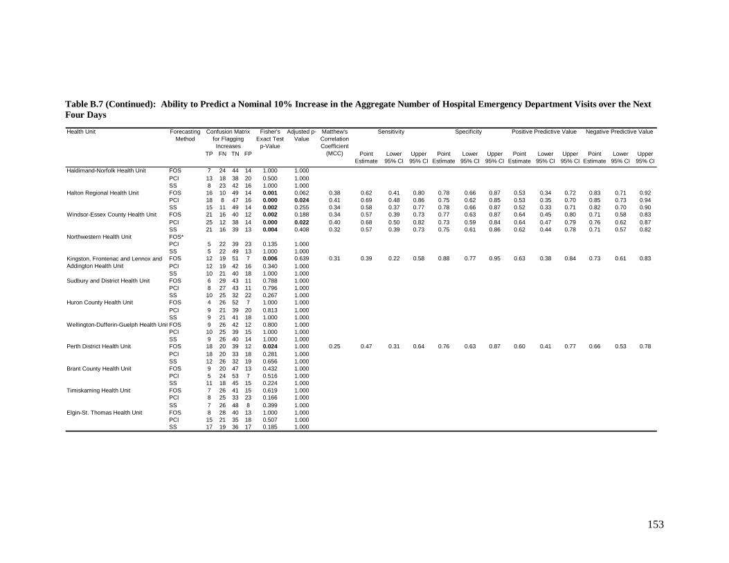
153
Table B.7 (Continued): Ability to Predict a Nominal 10% Increase in the Aggregate Number of Hospital Emergency Department Visits over the Next
Four Days
TP FN TN FP Point
Estimate
Lower
95% CI
Upper
95% CI
Point
Estimate
Lower
95% CI
Upper
95% CI
Point
Estimate
Lower
95% CI
Upper
95% CI
Point
Estimate
Lower
95% CI
Upper
95% CI
Haldimand-Norfolk Health Unit FOS 7 24 44 14 1.000 1.000 -0.02 0.23 0.10 0.41 0.76 0.63 0.86 0.33 0.15 0.57 0.65 0.52 0.76
Haldimand-Norfolk Health Unit PCI 13 18 38 20 0.500 1.000 0.07 0.42 0.25 0.61 0.66 0.52 0.78 0.39 0.23 0.58 0.68 0.54 0.80
Haldimand-Norfolk Health Unit SS 8 23 42 16 1.000 1.000 -0.02 0.26 0.12 0.45 0.72 0.59 0.83 0.33 0.16 0.55 0.65 0.52 0.76
Halton Regional Health Unit FOS 16 10 49 14 0.001 0.062 0.38 0.62 0.41 0.80 0.78 0.66 0.87 0.53 0.34 0.72 0.83 0.71 0.92
Halton Regional Health Unit PCI 18 8 47 16 0.000 0.024 0.41 0.69 0.48 0.86 0.75 0.62 0.85 0.53 0.35 0.70 0.85 0.73 0.94
Halton Regional Health Unit SS 15 11 49 14 0.002 0.255 0.34 0.58 0.37 0.77 0.78 0.66 0.87 0.52 0.33 0.71 0.82 0.70 0.90
Windsor-Essex County Health Unit FOS 21 16 40 12 0.002 0.188 0.34 0.57 0.39 0.73 0.77 0.63 0.87 0.64 0.45 0.80 0.71 0.58 0.83
Windsor-Essex County Health Unit PCI 25 12 38 14 0.000 0.022 0.40 0.68 0.50 0.82 0.73 0.59 0.84 0.64 0.47 0.79 0.76 0.62 0.87
Windsor-Essex County Health Unit SS 21 16 39 13 0.004 0.408 0.32 0.57 0.39 0.73 0.75 0.61 0.86 0.62 0.44 0.78 0.71 0.57 0.82
Northwestern Health Unit FOS* 3 24 57 5 0.694 1.000 0.05 0.11 0.02 0.29 0.92 0.82 0.97 0.38 0.09 0.76 0.70 0.59 0.80
Northwestern Health Unit PCI 5 22 39 23 0.135 1.000 -0.18 0.19 0.06 0.38 0.63 0.50 0.75 0.18 0.06 0.37 0.64 0.51 0.76
Northwestern Health Unit SS 5 22 49 13 1.000 1.000 -0.03 0.19 0.06 0.38 0.79 0.67 0.88 0.28 0.10 0.53 0.69 0.57 0.79
FOS 12 19 51 7 0.006 0.639 0.31 0.39 0.22 0.58 0.88 0.77 0.95 0.63 0.38 0.84 0.73 0.61 0.83
PCI 12 19 42 16 0.340 1.000 0.11 0.39 0.22 0.58 0.72 0.59 0.83 0.43 0.24 0.63 0.69 0.56 0.80
Kingston, Frontenac and Lennox and SS 10 21 40 18 1.000 1.000 0.01 0.32 0.17 0.51 0.69 0.55 0.80 0.36 0.19 0.56 0.66 0.52 0.77
Sudbury and District Health Unit FOS 6 29 43 11 0.788 1.000 -0.04 0.17 0.07 0.34 0.80 0.66 0.89 0.35 0.14 0.62 0.60 0.47 0.71
Sudbury and District Health Unit PCI 8 27 43 11 0.796 1.000 0.03 0.23 0.10 0.40 0.80 0.66 0.89 0.42 0.20 0.67 0.61 0.49 0.73
Sudbury and District Health Unit SS 10 25 32 22 0.267 1.000 -0.12 0.29 0.15 0.46 0.59 0.45 0.72 0.31 0.16 0.50 0.56 0.42 0.69
Huron County Health Unit FOS 4 26 52 7 1.000 1.000 0.02 0.13 0.04 0.31 0.88 0.77 0.95 0.36 0.11 0.69 0.67 0.55 0.77
Huron County Health Unit PCI 9 21 39 20 0.813 1.000 -0.04 0.30 0.15 0.49 0.66 0.53 0.78 0.31 0.15 0.51 0.65 0.52 0.77
Huron County Health Unit SS 9 21 41 18 1.000 1.000 -0.01 0.30 0.15 0.49 0.69 0.56 0.81 0.33 0.17 0.54 0.66 0.53 0.78
Wellington-Dufferin-Guelph Health Unit FOS 9 26 42 12 0.800 1.000 0.04 0.26 0.12 0.43 0.78 0.64 0.88 0.43 0.22 0.66 0.62 0.49 0.73
Wellington-Dufferin-Guelph Health PCI 10 25 39 15 1.000 1.000 0.01 0.29 0.15 0.46 0.72 0.58 0.84 0.40 0.21 0.61 0.61 0.48 0.73
Wellington-Dufferin-Guelph Health SS 9 26 40 14 1.000 1.000 0.00 0.26 0.12 0.43 0.74 0.60 0.85 0.39 0.20 0.61 0.61 0.48 0.72
Perth District Health Unit FOS 18 20 39 12 0.024 1.000 0.25 0.47 0.31 0.64 0.76 0.63 0.87 0.60 0.41 0.77 0.66 0.53 0.78
Perth District Health Unit PCI 18 20 33 18 0.281 1.000 0.12 0.47 0.31 0.64 0.65 0.50 0.78 0.50 0.33 0.67 0.62 0.48 0.75
Perth District Health Unit SS 12 26 32 19 0.656 1.000 -0.06 0.32 0.18 0.49 0.63 0.48 0.76 0.39 0.22 0.58 0.55 0.42 0.68
Brant County Health Unit FOS 9 20 47 13 0.432 1.000 0.10 0.31 0.15 0.51 0.78 0.66 0.88 0.41 0.21 0.64 0.70 0.58 0.81
Brant County Health Unit PCI 5 24 53 7 0.516 1.000 0.08 0.17 0.06 0.36 0.88 0.77 0.95 0.42 0.15 0.72 0.69 0.57 0.79
Brant County Health Unit SS 11 18 45 15 0.224 1.000 0.13 0.38 0.21 0.58 0.75 0.62 0.85 0.42 0.23 0.63 0.71 0.59 0.82
Timiskaming Health Unit FOS 7 26 41 15 0.619 1.000 -0.06 0.21 0.09 0.39 0.73 0.60 0.84 0.32 0.14 0.55 0.61 0.49 0.73
Timiskaming Health Unit PCI 8 25 33 23 0.166 1.000 -0.17 0.24 0.11 0.42 0.59 0.45 0.72 0.26 0.12 0.45 0.57 0.43 0.70
Timiskaming Health Unit SS 7 26 48 8 0.399 1.000 0.09 0.21 0.09 0.39 0.86 0.74 0.94 0.47 0.21 0.73 0.65 0.53 0.76
Elgin-St. Thomas Health Unit FOS 8 28 40 13 1.000 1.000 -0.03 0.22 0.10 0.39 0.75 0.62 0.86 0.38 0.18 0.62 0.59 0.46 0.71
Elgin-St. Thomas Health Unit PCI 15 21 35 18 0.507 1.000 0.08 0.42 0.26 0.59 0.66 0.52 0.78 0.45 0.28 0.64 0.63 0.49 0.75
Elgin-St. Thomas Health Unit SS 17 19 36 17 0.185 1.000 0.15 0.47 0.30 0.65 0.68 0.54 0.80 0.50 0.32 0.68 0.65 0.51 0.78
Matthew's
Correlation
Coefficient
(MCC)
Sensitivity Specificity Positive Predictive Value Negative Predictive ValueForecasting
Method
Confusion Matrix
for Flagging
Increases
Fisher's
Exact Test
p-Value
Adjusted p-
Value
Kingston, Frontenac and Lennox and
Addington Health Unit
Health Unit

154
Table B.8: Ability of Telehealth Ontario Calls to Directly Discriminate Between Increases in the
Aggregate Number of Hospital Emergency Department Visits Above a Nominal 10% Increase One
Week Ahead Health Unit AUROC Lower
95% CI
Upper 95%
CI
City of Toronto Health Unit 0.36 0.23 0.49
Grey Bruce Health Unit 0.49 0.34 0.64
Simcoe Muskoka District Health Unit 0.40 0.25 0.54
Niagara Regional Area Health Unit 0.44 0.31 0.57
Peel Regional Health Unit 0.49 0.36 0.62
City of Ottawa Health Unit 0.46 0.31 0.60
City of Hamilton Health Unit 0.41 0.28 0.54
York Regional Health Unit 0.34 0.23 0.46
Leeds, Grenville and Lanark District Health Unit 0.46 0.33 0.59
Middlesex-London Health Unit 0.41 0.29 0.54
Durham Regional Health Unit 0.34 0.22 0.47
The Eastern Ontario Health Unit 0.52 0.38 0.66
Peterborough County-City Health Unit 0.38 0.25 0.50
Hastings and Prince Edward Counties Health Unit 0.45 0.31 0.59
Waterloo Health Unit 0.39 0.27 0.51
The District of Algoma Health Unit 0.66 0.54 0.78
Renfrew County and District Health Unit 0.52 0.40 0.65
Thunder Bay District Health Unit 0.47 0.34 0.60
Porcupine Health Unit 0.47 0.34 0.59
Haliburton, Kawartha, Pine Ridge District Health Unit 0.40 0.27 0.52
North Bay Parry Sound District Health Unit 0.39 0.27 0.51
Oxford County Health Unit 0.45 0.33 0.58
Lambton Health Unit 0.50 0.37 0.62
Chatham-Kent Health Unit 0.56 0.42 0.70
Haldimand-Norfolk Health Unit 0.52 0.40 0.64
Halton Regional Health Unit 0.38 0.24 0.51
Windsor-Essex County Health Unit 0.48 0.35 0.60
Northwestern Health Unit 0.51 0.38 0.63
Kingston, Frontenac and Lennox and Addington Health Unit 0.53 0.40 0.66
Sudbury and District Health Unit 0.64 0.51 0.76
Huron County Health Unit 0.58 0.45 0.71
Wellington-Dufferin-Guelph Health Unit 0.56 0.44 0.69
Perth District Health Unit 0.44 0.32 0.57
Brant County Health Unit 0.46 0.33 0.58
Timiskaming Health Unit 0.49 0.37 0.62
Elgin-St. Thomas Health Unit 0.59 0.47 0.72

155
APPENDIX C: One-Week-Ahead Forecasts of the Weekly Aggregate Number of Hospital Emergency Visits for All Ontario Health Units

156
Figure C.1: One-Week-Ahead Forecasts of the Weekly Aggregate Number of Hospital Emergency
Visits using all Three Forecasting Methods and the Corresponding Weekly Aggregate Number of
Actual Visits for the (Approximate) City of Toronto Health Unit

157
Figure C.2: One-Week-Ahead Forecasts of the Weekly Aggregate Number of Hospital Emergency
Visits using all Three Forecasting Methods and the Corresponding Weekly Aggregate Number of
Actual Visits for the (Approximate) Grey Bruce Health Unit

158
Figure C.3: One-Week-Ahead Forecasts of the Weekly Aggregate Number of Hospital Emergency
Visits using all Three Forecasting Methods and the Corresponding Weekly Aggregate Number of
Actual Visits for the (Approximate) Simcoe Muskoka District Health Unit

159
Figure C.4: One-Week-Ahead Forecasts of the Weekly Aggregate Number of Hospital Emergency
Visits using all Three Forecasting Methods and the Corresponding Weekly Aggregate Number of
Actual Visits for the (Approximate) Niagara Regional Health Unit

160
Figure C.5: One-Week-Ahead Forecasts of the Weekly Aggregate Number of Hospital Emergency
Visits using all Three Forecasting Methods and the Corresponding Weekly Aggregate Number of
Actual Visits for the (Approximate) Peel Regional Health Unit

161
Figure C.6: One-Week-Ahead Forecasts of the Weekly Aggregate Number of Hospital Emergency
Visits using all Three Forecasting Methods and the Corresponding Weekly Aggregate Number of
Actual Visits for the (Approximate) City of Ottawa Health Unit

162
Figure C.7: One-Week-Ahead Forecasts of the Weekly Aggregate Number of Hospital Emergency
Visits using all Three Forecasting Methods and the Corresponding Weekly Aggregate Number of
Actual Visits for the (Approximate) City of Hamilton Health Unit

163
Figure C.8: One-Week-Ahead Forecasts of the Weekly Aggregate Number of Hospital Emergency
Visits using all Three Forecasting Methods and the Corresponding Weekly Aggregate Number of
Actual Visits for the (Approximate) York Regional Health Unit

164
Figure C.9: One-Week-Ahead Forecasts of the Weekly Aggregate Number of Hospital Emergency
Visits using all Three Forecasting Methods and the Corresponding Weekly Aggregate Number of
Actual Visits for the (Approximate) Leeds, Grenville and Lanark District Health Unit
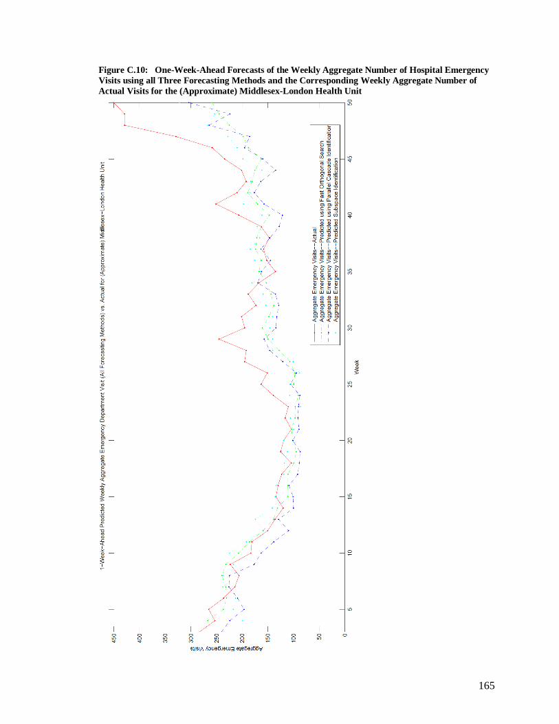
165
Figure C.10: One-Week-Ahead Forecasts of the Weekly Aggregate Number of Hospital Emergency
Visits using all Three Forecasting Methods and the Corresponding Weekly Aggregate Number of
Actual Visits for the (Approximate) Middlesex-London Health Unit

166
Figure C.11: One-Week-Ahead Forecasts of the Weekly Aggregate Number of Hospital Emergency
Visits using all Three Forecasting Methods and the Corresponding Weekly Aggregate Number of
Actual Visits for the (Approximate) Durham Regional Health Unit

167
Figure C.12: One-Week-Ahead Forecasts of the Weekly Aggregate Number of Hospital Emergency
Visits using all Three Forecasting Methods and the Corresponding Weekly Aggregate Number of
Actual Visits for the (Approximate) Eastern Ontario Health Unit

168
Figure C.13: One-Week-Ahead Forecasts of the Weekly Aggregate Number of Hospital Emergency
Visits using all Three Forecasting Methods and the Corresponding Weekly Aggregate Number of
Actual Visits for the (Approximate) Peterborough County-City Health Unit
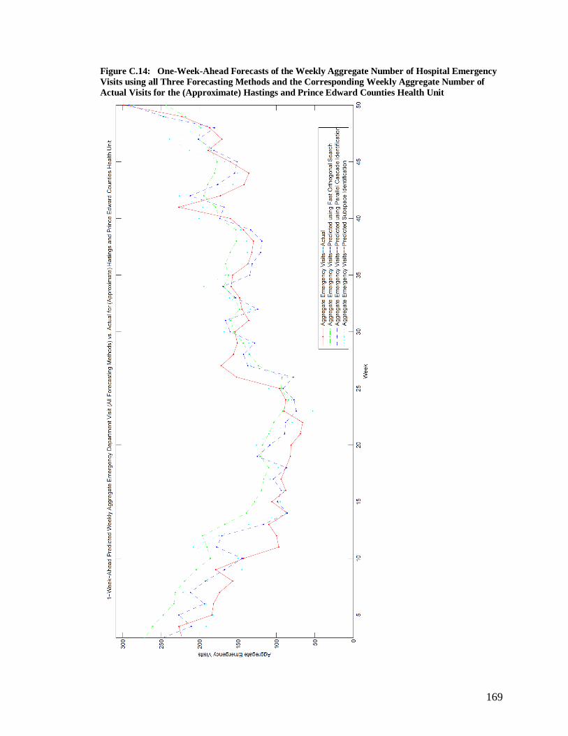
169
Figure C.14: One-Week-Ahead Forecasts of the Weekly Aggregate Number of Hospital Emergency
Visits using all Three Forecasting Methods and the Corresponding Weekly Aggregate Number of
Actual Visits for the (Approximate) Hastings and Prince Edward Counties Health Unit

170
Figure C.15: One-Week-Ahead Forecasts of the Weekly Aggregate Number of Hospital Emergency
Visits using all Three Forecasting Methods and the Corresponding Weekly Aggregate Number of
Actual Visits for the (Approximate) Waterloo Health Unit

171
Figure C.16: One-Week-Ahead Forecasts of the Weekly Aggregate Number of Hospital Emergency
Visits using all Three Forecasting Methods and the Corresponding Weekly Aggregate Number of
Actual Visits for the (Approximate) District of Algoma Health Unit
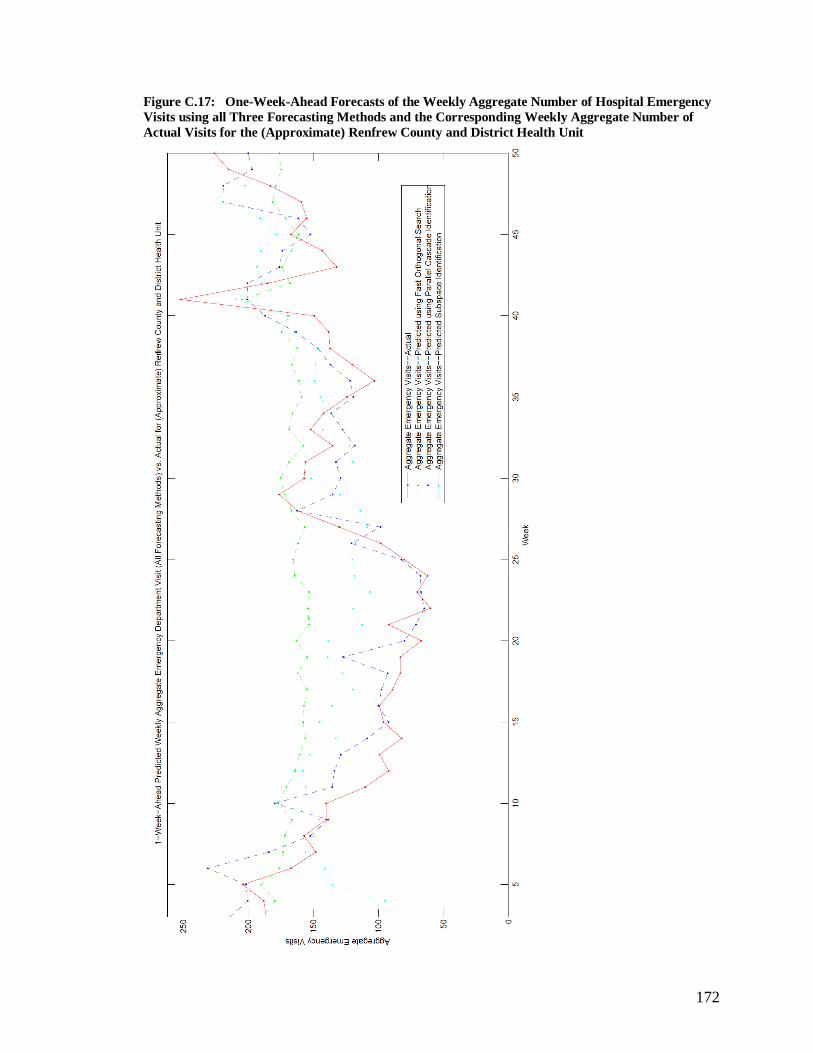
172
Figure C.17: One-Week-Ahead Forecasts of the Weekly Aggregate Number of Hospital Emergency
Visits using all Three Forecasting Methods and the Corresponding Weekly Aggregate Number of
Actual Visits for the (Approximate) Renfrew County and District Health Unit

173
Figure C.18: One-Week-Ahead Forecasts of the Weekly Aggregate Number of Hospital Emergency
Visits using all Three Forecasting Methods and the Corresponding Weekly Aggregate Number of
Actual Visits for the (Approximate) Thunder Bay Health Unit

174
Figure C.19: One-Week-Ahead Forecasts of the Weekly Aggregate Number of Hospital Emergency
Visits using all Three Forecasting Methods and the Corresponding Weekly Aggregate Number of
Actual Visits for the (Approximate) Porcupine Health Unit
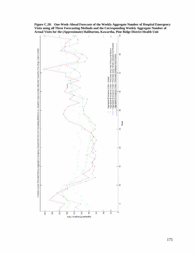
175
Figure C.20: One-Week-Ahead Forecasts of the Weekly Aggregate Number of Hospital Emergency
Visits using all Three Forecasting Methods and the Corresponding Weekly Aggregate Number of
Actual Visits for the (Approximate) Haliburton, Kawartha, Pine Ridge District Health Unit

176
Figure C.21: One-Week-Ahead Forecasts of the Weekly Aggregate Number of Hospital Emergency
Visits using all Three Forecasting Methods and the Corresponding Weekly Aggregate Number of
Actual Visits for the (Approximate) North Bay Parry Sound District Health Unit

177
Figure C.22: One-Week-Ahead Forecasts of the Weekly Aggregate Number of Hospital Emergency
Visits using all Three Forecasting Methods and the Corresponding Weekly Aggregate Number of
Actual Visits for the (Approximate) Oxford County Health Unit
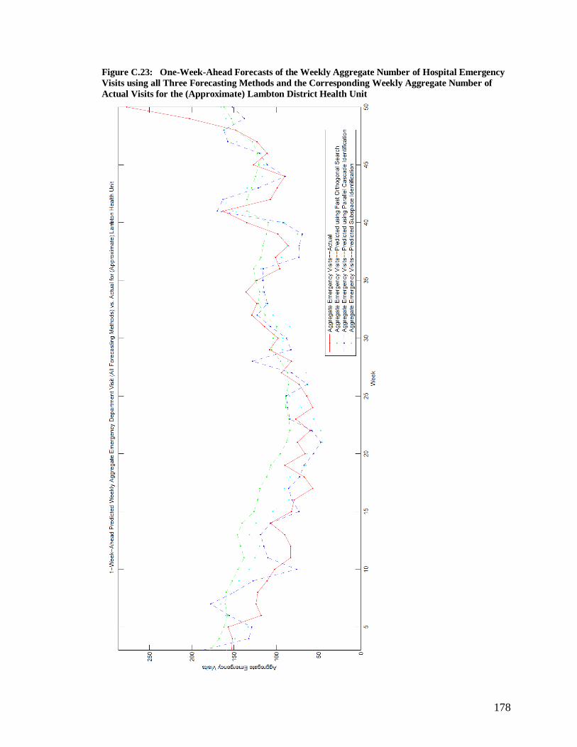
178
Figure C.23: One-Week-Ahead Forecasts of the Weekly Aggregate Number of Hospital Emergency
Visits using all Three Forecasting Methods and the Corresponding Weekly Aggregate Number of
Actual Visits for the (Approximate) Lambton District Health Unit

179
Figure C.24: One-Week-Ahead Forecasts of the Weekly Aggregate Number of Hospital Emergency
Visits using all Three Forecasting Methods and the Corresponding Weekly Aggregate Number of
Actual Visits for the (Approximate) Chatham-Kent Health Unit

180
Figure C.25: One-Week-Ahead Forecasts of the Weekly Aggregate Number of Hospital Emergency
Visits using all Three Forecasting Methods and the Corresponding Weekly Aggregate Number of
Actual Visits for the (Approximate) Haldimand-Norfolk Health Unit

181
Figure C.26: One-Week-Ahead Forecasts of the Weekly Aggregate Number of Hospital Emergency
Visits using all Three Forecasting Methods and the Corresponding Weekly Aggregate Number of
Actual Visits for the (Approximate) Halton Regional Unit

182
Figure C.27: One-Week-Ahead Forecasts of the Weekly Aggregate Number of Hospital Emergency
Visits using all Three Forecasting Methods and the Corresponding Weekly Aggregate Number of
Actual Visits for the (Approximate) Windsor-Essex County Health Unit

183
Figure C.28: One-Week-Ahead Forecasts of the Weekly Aggregate Number of Hospital Emergency
Visits using all Three Forecasting Methods and the Corresponding Weekly Aggregate Number of
Actual Visits for the (Approximate) Northwestern Health Unit

184
Figure C.29: One-Week-Ahead Forecasts of the Weekly Aggregate Number of Hospital Emergency
Visits using all Three Forecasting Methods and the Corresponding Weekly Aggregate Number of
Actual Visits for the (Approximate) Kingston, Frontenac and Lennox and Addington Health Unit

185
Figure C.30: One-Week-Ahead Forecasts of the Weekly Aggregate Number of Hospital Emergency
Visits using all Three Forecasting Methods and the Corresponding Weekly Aggregate Number of
Actual Visits for the (Approximate) Sudbury and District Health Unit

186
Figure C.31: One-Week-Ahead Forecasts of the Weekly Aggregate Number of Hospital Emergency
Visits using all Three Forecasting Methods and the Corresponding Weekly Aggregate Number of
Actual Visits for the (Approximate) Huron County Health Unit
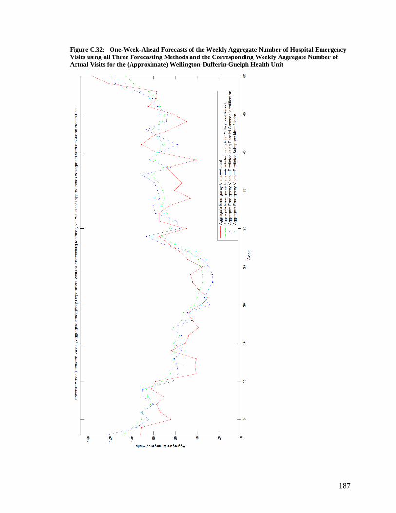
187
Figure C.32: One-Week-Ahead Forecasts of the Weekly Aggregate Number of Hospital Emergency
Visits using all Three Forecasting Methods and the Corresponding Weekly Aggregate Number of
Actual Visits for the (Approximate) Wellington-Dufferin-Guelph Health Unit

188
Figure C.33: One-Week-Ahead Forecasts of the Weekly Aggregate Number of Hospital Emergency
Visits using all Three Forecasting Methods and the Corresponding Weekly Aggregate Number of
Actual Visits for the (Approximate) Perth District Health Unit

189
Figure C.34: One-Week-Ahead Forecasts of the Weekly Aggregate Number of Hospital Emergency
Visits using all Three Forecasting Methods and the Corresponding Weekly Aggregate Number of
Actual Visits for the (Approximate) Brant County Health Unit

190
Figure C.35: One-Week-Ahead Forecasts of the Weekly Aggregate Number of Hospital Emergency
Visits using all Three Forecasting Methods and the Corresponding Weekly Aggregate Number of
Actual Visits for the (Approximate) Timiskaming Health Unit

191
Figure C.36: One-Week-Ahead Forecasts of the Weekly Aggregate Number of Hospital Emergency
Visits using all Three Forecasting Methods and the Corresponding Weekly Aggregate Number of
Actual Visits for the (Approximate) Elgin-St. Thomas Health Unit