NATIONAL ELECTRICITY FORECASTING REPORT
188
NATIONAL ELECTRICITY FORECASTING REPORT For the National Electricity Market (NEM) 2012
Transcript of NATIONAL ELECTRICITY FORECASTING REPORT

NATIONAL ELECTRICITY FORECASTING REPORT
For the National Electricity Market (NEM)
2012

NATIONAL ELECTRICITY FORECASTING REPORT
ii © AEMO 2012
Disclaimer This document is subject to an important disclaimer that limits or excludes AEMO’s liability.
Please read the full disclaimer on page D1.
Published by
AEMO Australian Energy Market Operator ABN 94 072 010 327 Copyright © 2012 AEMO

© AEMO 2012 Foreword iii
FOREWORD
This is the first edition of AEMO’s National Electricity Forecasting Report (NEFR), which represents the first time AEMO has developed independent electricity demand forecasts on a consistent basis for the five National Electricity Market (NEM) regions, namely New South Wales (including the Australian Capital Territory), Queensland, South Australia, Tasmania, and Victoria.
National Electricity Forecasting represents a package of information papers and reports that document the input data, assumptions, and methodology used to develop a set of annual energy and maximum demand forecasts for the NEM, ensuring an open and transparent process. This will then allow AEMO to engage and work collaboratively with stakeholders to ensure continued efficiency in terms of NEM operations.
In the past, AEMO has published demand forecasts via a series of AEMO planning publications, namely the Electricity Statement of Opportunities (ESOO), the Victorian Annual Planning Report (VAPR), and the South Australian Supply and Demand Outlook (SASDO).
From 2012, the NEFR will be the only AEMO publication presenting electricity demand forecasts for the NEM.
Robust independent forecasting is needed to assist AEMO with planning efficient future investment in electricity infrastructure to service the long-term needs of energy consumers. These forecasts are used for both operational purposes, including the calculation of marginal loss factors, and as a key input into AEMO’s national transmission planning role.
Significant factors currently influencing changes in demand involve the penetration of rooftop photovoltaic systems, changing consumption patterns in the industrial sector (particularly in mining and manufacturing), consumer responses to rising electricity prices and energy efficiency initiatives, and changes in domestic and international economics.
In the second half of 2012, AEMO will be holding regional forums that will promote further dialogue with stakeholders, with an aim to discuss the forecasts and assumptions related to National Electricity Forecasting. This will also provide an opportunity for stakeholders to be involved in discussions about the future direction of NEM forecasting.
I look forward to working more closely with our stakeholders to ensure this forecasting process is a success.
Matt Zema
Managing Director and Chief Executive Officer

NATIONAL ELECTRICITY FORECASTING REPORT
iv Foreword © AEMO 2012
[This page is left blank intentionally]

© AEMO 2012 Executive summary v
EXECUTIVE SUMMARY
Annual energy and maximum demand forecasts are significantly lower than those contained in the 2011 ESOO, signalling an expected delay for new generation and network investment.
To benefit the long-term needs of energy consumers, robust independent forecasting of electricity supply and consumption is needed to assist with planning future efficient investment.
For the first time AEMO has developed an independent set of electricity forecasts for each region of the National Electricity Market (NEM) to capture and assess the notable changes taking place.
AEMO will be using the National Electricity Forecasting Report as a basis for further collaboration with our stakeholders to maintain the quality and value of this work.
Key observations for the 2012 National Electricity Forecasts detailed in this report are as follows:
• Across the NEM, annual energy for 2011-12 is projected to be 2.4 per cent lower than 2010-11 and 5.7 per cent lower than forecast in the 2011 ESOO under a “medium” economic growth scenario.
• Forecast annual energy for 2012-13 is projected to remain flat (0.0% growth), which represents an 8.8 per cent reduction from the 2011 ESOO forecast.
• Average growth in annual energy for the 10-year period is now forecast to be 1.7 per cent, down from the 2.3 per cent forecast in the 2011 ESOO.
• Growth in annual energy consumption is strongly linked to large industrial projects in Queensland, most notably coal seam gas developments.
• Maximum demand forecasts across the five regions are much lower than in previous years, but are expected to continue to grow into the future.
The main factors influencing these changes are as follows:
• Changes in the economic outlook. Reduced energy forecasts are consistent with a moderation in gross domestic product (GDP), especially in the short term.
• Reduced manufacturing consumption in response to the high Australian dollar. An expected increase in cheaper imports is anticipated to impact domestic manufacturing growth.
• Significant penetration of rooftop PV systems (South Australia has the highest penetration of rooftop PV of all the NEM states). The impact of rooftop PV installations is expected to partially offset the need for increased electricity generation. By 2021-22, this is forecast to increase to 7,558 GWh or 3.4% of annual energy.
• Consumer response (commercial and residential) to rising electricity costs and energy efficiency measures.
Future implications
Structural change in the Australian economy – acceleration in the mining sector in the northern states together with a decline in manufacturing in Victoria, South Australia and Tasmania – is having disparate impacts across the NEM states, particularly in the wake of the global financial crisis.
Across the NEM, lower than forecast annual energy for 2011-12 under a “medium” economic growth scenario points to a likely delay in the need for new generation investment including the potential for a reduction in significant large-scale investment.

NATIONAL ELECTRICITY FORECASTING REPORT
vi Executive summary © AEMO 2012
Figure 1 — Revised annual energy growth rates
NSW QLD SA TAS VIC NEM2011 ESOO 1.6% 4.1% 1.5% 0.9% 1.6% 2.3%2012 NEFR 1.2% 2.9% 0.9% 0.9% 1.4% 1.7%
0.0%
0.5%
1.0%
1.5%
2.0%
2.5%
3.0%
3.5%
4.0%
4.5%
Annu
al a
vera
ge g
row
th ra
te to
202
1-22
-An
nual
ene
rgy (
GW
h)

© AEMO 2012 Executive summary vii
Figure 2 — Revised maximum demand growth rates
NSW QLD SA TAS VIC2011 ESOO 1.9% 4.2% 1.7% 1.4% 2.1%2012 NEFR 1.2% 2.5% 1.0% 1.1% 1.6%
0.0%
0.5%
1.0%
1.5%
2.0%
2.5%
3.0%
3.5%
4.0%
4.5%
Annu
al a
vera
ge g
row
th ra
te to
202
1-22
-M
axim
um d
eman
d (M
W)

NATIONAL ELECTRICITY FORECASTING REPORT
viii Executive summary © AEMO 2012
[This page is left blank intentionally]

© AEMO 2012 Contents ix
CONTENTS
FOREWORD III
EXECUTIVE SUMMARY V
CHAPTER 1 - INTRODUCTION 1-1
1.1 National Electricity Forecasting 1-1 1.2 The NEFR and AEMO’s other planning publications 1-2 1.3 Content and structure of the NEFR 1-3
CHAPTER 2 - DEFINITIONS, PROCESS AND METHODOLOGY 2-1
2.1 Key definitions of energy and maximum demand 2-1 2.1.1 Energy and maximum demand definitions 2-1 2.1.2 The components of energy and maximum demand in NEM forecasting 2-3
2.2 Process and methodology 2-5 2.2.1 Overview of the AEMO forecasting process 2-5 2.2.2 NTNDP scenarios 2-7 2.2.3 Mapping the NTNDP scenarios 2-8
2.3 Changes since the 2011 ESOO 2-9
CHAPTER 3 - NEM-WIDE FORECASTS 3-1
Summary 3-1 3.1 Annual energy forecasts 3-2
3.1.1 Annual energy forecasts 3-2 3.1.2 Mass market forecasts 3-6 3.1.3 Large industrial forecasts 3-7 3.1.4 Annual electrical energy requirement breakdown 3-8
3.2 Maximum demand forecasts 3-8 3.3 Small non-scheduled generation forecasts 3-9
CHAPTER 4 - NEW SOUTH WALES (INCLUDING ACT) FORECASTS 4-1
Summary 4-1 4.1 Annual energy forecasts 4-2
4.1.1 Annual energy forecasts 4-2 4.1.2 Mass market forecasts 4-6 4.1.3 Large industrial forecasts 4-7 4.1.4 Annual electrical energy requirement breakdown 4-8
4.2 Maximum demand forecasts 4-9 4.2.1 Summer maximum demand forecasts 4-9 4.2.2 Winter maximum demand forecasts 4-12
4.3 Small non-scheduled generation forecasts 4-14

NATIONAL ELECTRICITY FORECASTING REPORT
x Contents © AEMO 2012
CHAPTER 5 - QUEENSLAND FORECASTS 5-1
Summary 5-1 5.1 Annual energy forecasts 5-2
5.1.1 Annual energy forecasts 5-2 5.1.2 Mass market forecasts 5-6 5.1.3 Large industrial forecasts 5-7 5.1.4 Annual electrical energy requirement breakdown 5-9
5.2 Maximum demand forecasts 5-10 5.2.1 Summer maximum demand forecasts 5-10 5.2.2 Winter maximum demand forecasts 5-13
5.3 Small non-scheduled generation forecasts 5-16
CHAPTER 6 - SOUTH AUSTRALIA FORECASTS 6-1
Summary 6-1 6.1 Annual energy forecasts 6-2
6.1.1 Annual energy forecasts 6-2 6.1.2 Mass market forecasts 6-6 6.1.3 Large industrial forecasts 6-7 6.1.4 Annual electrical energy requirement breakdown 6-8
6.2 Maximum demand forecasts 6-9 6.2.1 Summer maximum demand forecasts 6-9 6.2.2 Winter maximum demand forecasts 6-12
6.3 Small non-scheduled generation forecasts 6-14
CHAPTER 7 - TASMANIA FORECASTS 7-1
Summary 7-1 7.1 Annual energy forecasts 7-2
7.1.1 Annual energy forecasts 7-2 7.1.2 Mass market forecasts 7-6 7.1.3 Large industrial forecasts 7-7 7.1.4 Annual electrical energy requirement breakdown 7-8
7.2 Maximum demand forecasts 7-9 7.2.1 Summer maximum demand forecasts 7-9 7.2.2 Winter maximum demand forecasts 7-12
7.3 Small non-scheduled generation forecasts 7-14
CHAPTER 8 - VICTORIA FORECASTS 8-1
Summary 8-1 8.1 Annual energy forecasts 8-2
8.1.1 Annual energy forecasts 8-2 8.1.2 Mass market forecasts 8-6 8.1.3 Large industrial forecasts 8-7 8.1.4 Annual electrical energy requirement breakdown 8-8
8.2 Maximum demand forecasts 8-8 8.2.1 Summer maximum demand forecasts 8-8 8.2.2 Winter maximum demand forecasts 8-12
© AEMO 2012 Contents xi
8.3 Small non-scheduled generation forecasts 8-14
APPENDIX A - REGIONAL MODEL EQUATIONS FOR NON-LARGE INDUSTRIAL CONSUMPTION A-1
A.1 New South Wales (including the ACT) A-1 A.2 Queensland A-2 A.3 South Australia A-3 A.4 Tasmania A-4 A.5 Victoria A-5
APPENDIX B - ENERGY EFFICIENCY B-1
B.1 Introduction B-1 B.1.1 Energy efficiency impacts as a post-model adjustment B-1 B.1.2 Energy efficiency definition B-1 B.1.3 Impacts on demand forecasting B-1 B.1.4 Future work B-2
B.2 Energy efficiency policies, drivers and methodology B-2 B.2.1 Energy efficiency policies B-2
B.3 Drivers of energy efficiency B-4 B.4 Energy efficiency impact forecast category B-5 B.5 Energy efficiency impact base scenario and data sources B-5 B.6 Estimating energy efficiency policy impacts B-5 B.7 Modelling limitations B-7 B.8 Energy efficiency policy impacts in the NEM B-7 B.9 Historical analysis B-7 B.10 Annual energy B-8 B.11 Maximum demand B-9 B.12 Regional energy efficiency policy impact B-10
B.12.1 New South Wales (and the Australian Capital Territory) B-10 B.12.2 Queensland B-13 B.12.3 South Australia B-15 B.12.4 Tasmania B-18 B.12.5 Victoria B-20
B.13 National energy efficiency policies B-22 B.13.1 Clean Energy Future Plan B-22 B.13.2 Renewable Energy Target B-23 B.13.3 Energy Efficiency Opportunities Regulations B-23 B.13.4 Residential and commercial building mandatory disclosure B-23 B.13.5 Minimum Energy Performance Standards B-24 B.13.6 Energy Efficiency Building Standards B-24 B.13.7 Phase-out of Electric Storage Hot Water Systems and Solar Hot Water Rebate B-26
B.14 State energy efficiency policies B-26 B.14.1 New South Wales Energy Savings Scheme B-26 B.14.2 Queensland Renewable Energy Plan 2012 B-27 B.14.3 South Australia Residential Energy Efficiency Scheme (REES) B-27 B.14.4 Victorian Energy Efficiency Target B-28

NATIONAL ELECTRICITY FORECASTING REPORT
xii Contents © AEMO 2012
APPENDIX C - SMALL NON-SCHEDULED GENERATION C-1
C.1 New South Wales C-1 C.2 Queensland C-4 C.3 South Australia C-7 C.4 Tasmania C-9 C.5 Victoria C-11
APPENDIX D - DEMAND-SIDE PARTICIPATION D-1
D.1 Survey and analysis of results D-1 D.2 Demand-side participation forecasts D-2 D.3 Treatment of demand-side participation in the maximum demand projections D-3
DISCLAIMER D1
MEASURES AND ABBREVIATIONS M1
Units of measure M1 Abbreviations M2
GLOSSARY AND LIST OF COMPANY NAMES G1
Glossary G1 List of company names G7

© AEMO 2012 Tables xiii
TABLES Table 2-1 — Mapping scenarios for national electricity forecasting 2-9 Table 2-2 — Energy projection changes since the 2011 ESOO 2-10 Table 2-3 — Summer 10% POE maximum demand projection changes since the 2011 ESOO 2-10 Table 2-4 — Winter 10% POE maximum demand projection changes since the 2011 ESOO 2-10 Table 3-1 — NEM annual energy forecasts (GWh) 3-4 Table 3-2 — NEM-wide annual electrical energy requirement breakdown (GWh) 3-8 Table 3-3 — Forecasts of small non-scheduled generation energy for the NEM (GWh) 3-10 Table 4-1 — Annual energy forecasts for New South Wales (including the ACT) (GWh) 4-4 Table 4-2 — Annual electrical energy requirement breakdown for New South Wales (including the ACT) (GWh) 4-8 Table 4-3 — Summer maximum demand forecasts for New South Wales (including the ACT) 4-10 Table 4-4 — Winter maximum demand forecasts for New South Wales (including the ACT) (MW) 4-13 Table 4-5 — Forecasts of small non-scheduled generation energy for New South Wales (including ACT) (GWh) 4-15 Table 4-6 — Forecasts of the small non-scheduled generation contribution to maximum demand for New South
Wales (including ACT) (MW) 4-16 Table 5-1 — Annual energy forecasts for Queensland (GWh) 5-4 Table 5-2 — Annual electrical energy requirement breakdown for Queensland (GWh) 5-9 Table 5-3 — Summer maximum demand forecasts for Queensland (MW) 5-11 Table 5-4 — Winter maximum demand forecasts for Queensland (MW) 5-14 Table 5-5 — Forecasts of small non-scheduled generation energy for Queensland (GWh) 5-17 Table 5-6 — Forecasts of the small non-scheduled generation contribution to maximum demand for Queensland
(MW) 5-18 Table 6-1 — Annual energy forecasts for South Australia (GWh) 6-4 Table 6-2 — Annual electrical energy requirement breakdown for South Australia (GWh) 6-8 Table 6-3 — Summer maximum demand forecasts for South Australia (MW) 6-10 Table 6-4 — Winter maximum demand forecasts for South Australia (MW) 6-13 Table 6-5 — Forecasts of small non-scheduled generation energy for South Australia (GWh) 6-15 Table 6-6 — Forecasts of the small non-scheduled generation contribution to maximum demand for South
Australia (MW) 6-16 Table 7-1 — Annual energy forecasts for Tasmania (GWh) 7-4 Table 7-2 — Annual electrical energy requirement breakdown for Tasmania (GWh) 7-8 Table 7-3 — Summer maximum demand forecasts for Tasmania (MW) 7-10 Table 7-4 — Winter maximum demand forecasts for Tasmania (MW) 7-13 Table 7-5 — Forecasts of small non-scheduled generation energy for Tasmania (GWh) 7-15 Table 7-6 — Forecasts of the small non-scheduled generation contribution to maximum demand for Tasmania
(MW) 7-16 Table 8-1 — Annual energy forecasts for Victoria (GWh) 8-4 Table 8-2 — Annual electrical energy requirement breakdown for Victoria (GWh) 8-8 Table 8-3 — Summer maximum demand forecasts for Victoria (MW) 8-10 Table 8-4 — Winter maximum demand forecasts for Victoria (MW) 8-13 Table 8-5 — Forecasts of small non-scheduled generation energy for Victoria (GWh) 8-15 Table 8-6 — Forecasts of the small non-scheduled generation contribution to maximum demand for Victoria
(MW) 8-16 Table B-1 — Key national policies that may impact NEM electricity demand B-3 Table B-2 — Key state policies that may impact NEM electricity demand B-4 Table B-3 — Estimated average daily consumption per household in kWh by NEM region in 2004–05, 2007–08
and 2010–11 B-8 Table B-4 — State building standards B-25 Table B-5 — Energy Savings Scheme B-27 Table B-6 — Annual greenhouse gas reduction targets for REES stage 1 and 2 (CO2-e tonnes) B-28

NATIONAL ELECTRICITY FORECASTING REPORT
xiv Figures © AEMO 2012
Table C-1 — List of power stations used for operational demand forecasts for New South Wales (including ACT)C-1 Table C-2 — List of power stations used for annual energy forecasts for New South Wales (including ACT) C-2 Table C-3 — List of power stations used for operational demand forecasts for Queensland C-4 Table C-4 — List of power stations used for annual energy forecasts for Queensland C-5 Table C-5 — List of power stations used for operational demand forecasts for South Australia C-7 Table C-6 — List of power stations used for annual energy forecasts for South Australia C-8 Table C-7 — List of power stations used for operational demand forecasts for Tasmania C-9 Table C-8 — List of power stations used for annual energy forecasts for Tasmania C-10 Table C-9 — List of power stations used for operational demand forecasts for Victoria C-11 Table C-10 — List of power stations used for annual energy forecasts for Victoria C-12 Table D-1 — Estimated historical DSP (MW) D-2 Table D-2 — DSP available for the 2012-13 summer (MW) D-2 Table D-3 — Future scenarios for DSP (annual growth) D-3
FIGURES Figure 1 — Revised annual energy growth rates vi Figure 2 — Revised maximum demand growth rates vii Figure 1-1 — AEMO’s national electricity forecasting 1-2 Figure 1-2 — Forecasts as inputs into AEMO publications and processes 1-3 Figure 2-1 — Electricity network topology 2-2 Figure 2-2 — The components of energy and maximum demand 2-4 Figure 2-3 — Overview of forecasting process 2-6 Figure 3-1 — Annual energy forecasts for the NEM 3-3 Figure 3-2 — Comparison of the 2012 NEFR and 2011 ESOO annual energy forecasts for the NEM 3-5 Figure 3-3 — Mass market forecasts for the NEM 3-6 Figure 3-4 — Large industrial forecasts for the NEM 3-7 Figure 4-1 — Annual energy forecasts for New South Wales (including the ACT) 4-3 Figure 4-2 — Comparison of the 2012 NEFR and 2011 ESOO annual energy forecasts for New South Wales
(including the ACT) 4-5 Figure 4-3 — Mass market forecasts for New South Wales (including the ACT) 4-6 Figure 4-4 — Large industrial forecasts for New South Wales (including the ACT) 4-7 Figure 4-5 — Summer 50% POE maximum demand forecasts for New South Wales (including the ACT) 4-9 Figure 4-6 — Comparison of the 2012 NEFR and 2011 ESOO summer maximum demand forecasts for New
South Wales (including the ACT) 4-11 Figure 4-7 — Winter 50% POE maximum demand forecasts for New South Wales (including the ACT) 4-12 Figure 4-8 — Comparison of the 2012 NEFR and 2011 ESOO winter maximum demand forecasts for New South
Wales (including the ACT) 4-14 Figure 5-1 — Annual energy forecasts for Queensland 5-3 Figure 5-2 — Comparison of the 2012 NEFR and 2011 ESOO annual energy forecasts for Queensland 5-5 Figure 5-3 — Mass market forecasts for Queensland 5-6 Figure 5-4 — Large industrial forecasts for Queensland 5-8 Figure 5-5 — Summer 50% POE maximum demand forecasts for Queensland 5-10 Figure 5-6 — Comparison of the 2012 NEFR and 2011 ESOO summer maximum demand forecasts for
Queensland 5-12 Figure 5-7 — Winter 50% POE maximum demand forecasts for Queensland 5-13 Figure 5-8 — Comparison of the 2012 NEFR and 2011 ESOO winter maximum demand forecasts for
Queensland 5-15 Figure 6-1 — Annual energy forecasts for South Australia 6-3

© AEMO 2012 Figures xv
Figure 6-2 — Comparison of the 2012 NEFR and 2011 ESOO annual energy forecasts for South Australia 6-5 Figure 6-3 — Mass market forecasts for South Australia 6-6 Figure 6-4 — Large industrial forecasts for South Australia 6-7 Figure 6-5 — Summer 50% POE maximum demand forecasts for South Australia 6-9 Figure 6-6 — Comparison of the 2012 NEFR and 2011 ESOO summer maximum demand forecasts for South
Australia 6-11 Figure 6-7 — Winter 50% POE maximum demand forecasts for South Australia 6-12 Figure 6-8 — Comparison of the 2012 NEFR and 2011 ESOO forecasts for South Australia 6-14 Figure 7-1 — Annual energy forecasts for Tasmania 7-3 Figure 7-2 — Comparison of the 2012 NEFR and 2011 ESOO annual energy forecasts for Tasmania 7-5 Figure 7-3 — Mass market forecasts for Tasmania 7-6 Figure 7-4 — Large industrial forecasts for Tasmania 7-7 Figure 7-5 — Summer 50% POE maximum demand forecasts for Tasmania 7-9 Figure 7-6 — Comparison of the 2012 NEFR and 2011 ESOO summer maximum demand forecasts for
Tasmania 7-11 Figure 7-7 — Winter 50% POE maximum demand forecasts for Tasmania 7-12 Figure 7-8 — Comparison of the 2012 NEFR and 2011 ESOO winter maximum demand forecasts for Tasmania7-14 Figure 8-1 — Annual energy forecasts for Victoria 8-3 Figure 8-2 — Comparison of the 2012 NEFR and 2011 ESOO annual energy forecasts for Victoria 8-5 Figure 8-3 — Mass market forecasts for Victoria 8-6 Figure 8-4 — Large industrial forecasts for Victoria 8-7 Figure 8-5 — Summer 50% POE maximum demand forecasts for Victoria 8-9 Figure 8-6 — Comparison of the 2012 NEFR and 2011 ESOO summer maximum demand forecasts for Victoria8-11 Figure 8-7 — Winter 50% POE maximum demand forecasts for Victoria 8-12 Figure 8-8 — Comparison of the 2012 NEFR and 2011 ESOO winter maximum demand forecasts for Victoria 8-14 Figure B-1 — Modelling framework for the policy impact forecast B-6 Figure B-2 — Residential electricity consumption by appliance in the NEM B-8 Figure B-3 — Energy efficiency policy, annual energy impact forecasts by NEM region B-9 Figure B-4 — Energy efficiency policy, summer maximum demand impact forecasts by NEM region B-10 Figure B-5 — Energy efficiency impact annual energy forecasts for New South Wales (and the Australian Capital
Territory) B-11 Figure B-6 — Energy efficiency impact summer maximum demand forecasts for New South Wales (and the
Australian Capital Territory) B-12 Figure B-7 — Energy efficiency impact winter maximum demand forecasts for New South Wales (and the
Australian Capital Territory) B-12 Figure B-8 — Energy efficiency impact annual energy forecasts for Queensland B-13 Figure B-9 — Energy efficiency impact summer maximum demand forecasts for Queensland B-14 Figure B-10 — Energy efficiency impact winter maximum demand forecasts for Queensland B-15 Figure B-11 — Energy efficiency impact annual energy forecasts for South Australia B-16 Figure B-12 — Energy efficiency impact summer maximum demand forecasts for South Australia B-17 Figure B-13 — Energy efficiency impact winter maximum demand forecasts for South Australia B-17 Figure B-14 — Energy efficiency impact annual energy forecasts for Tasmania B-18 Figure B-15 — Energy efficiency impact summer maximum demand forecasts for Tasmania B-19 Figure B-16 — Energy efficiency impact winter maximum demand forecasts for Tasmania B-19 Figure B-17 — Energy efficiency impact annual energy forecasts for Victoria B-20 Figure B-18 — Energy efficiency impact summer maximum demand forecasts for Victoria B-21 Figure B-19 — Energy efficiency impact winter maximum demand forecasts for Victoria B-21 Figure D-1 — Overview of forecasting process D-3

NATIONAL ELECTRICITY FORECASTING REPORT
xvi Figures © AEMO 2012
[This page is left blank intentionally]

© AEMO 2012 Introduction 1-1
CHAPTER 1 - INTRODUCTION
1.1 National Electricity Forecasting AEMO has changed the way it develops and publishes electricity demand forecasts for the electricity industry, by developing independent forecasts for each region in the National Electricity Market (NEM).
Electricity demand forecasts are used for operational purposes, for the calculation of marginal loss factors, and as a key input into AEMO‘s national transmission planning role. This requires a close understanding of how the forecasts are developed to ensure forecasting processes and assumptions are consistently applied and fit for purpose. AEMO is ideally positioned to undertake this task and lead collaboration with the industry to ensure representative and reliable forecasts are consistently produced for each region.
Previously, AEMO developed demand forecasts for South Australia and Victoria, while the regional transmission network service providers (TNSPs) developed forecasts for Queensland, New South Wales (including the Australian Capital Territory), and Tasmania. These forecasts were subsequently published via a series of AEMO publications including the Electricity Statement of Opportunities (ESOO), the Victorian Annual Planning Report (VAPR), and the South Australian Supply and Demand Outlook (SASDO).
National electricity forecasting
To facilitate greater forecasting transparency and stimulate discussion with the electricity industry, AEMO is now publishing the electricity demand forecasts via a series of separate information papers and reports:
• Economic Outlook Information Paper is AEMO’s assessment of the work undertaken by the National Institute of Economic and Industry Research (NIEIR), published in May 2012.
• Rooftop PV Information Paper quantifies the impact of rooftop photovoltaic (PV) systems on the electricity market, published in May 2012.
• 2011–12 NEM Demand Review Information Paper reviews 2011–12 NEM demand.
• Forecasting Methodology Information Paper describes the modelling process underpinning the demand forecast development.
• 2012 National Electricity Forecasting Report (NEFR) presents the electricity demand forecasts for the five NEM regions.
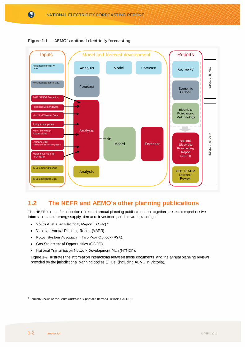
Figure 1-1 illustrates the inputs, the modelling and forecast development processes, and the subsequent reports underpinning AEMO’s new approach to national electricity forecasting.
This is first time AEMO has developed forecasts for the NEM, so more work still needs to be done, and AEMO will continue to improve the underpinning data, modelling, and interpretation, as well as engaging with industry on an ongoing basis to ensure an open and transparent process.
NATIONAL ELECTRICITY FORECASTING REPORT
1-2 Introduction © AEMO 2012
Figure 1-1 — AEMO’s national electricity forecasting
1.2 The NEFR and AEMO’s other planning publications The NEFR is one of a collection of related annual planning publications that together present comprehensive information about energy supply, demand, investment, and network planning:
• South Australian Electricity Report (SAER).1
• Victorian Annual Planning Report (VAPR).
• Power System Adequacy – Two Year Outlook (PSA).
• Gas Statement of Opportunities (GSOO).
• National Transmission Network Development Plan (NTNDP).
Figure 1-2 illustrates the information interactions between these documents, and the annual planning reviews provided by the jurisdictional planning bodies (JPBs) (including AEMO in Victoria).
1 Formerly known as the South Australian Supply and Demand Outlook (SASDO).
2011-12 NEM Demand Review
Analysis
Rooftop PV
Economic Outlook
May 2012 release
June 2012 release
ForecastNational Electricity
Forecasting Report (NEFR)
Model and forecast development Reports
Model
Electricity Forecasting Methodology
ForecastModelAnalysis
Analysis
Forecast
Historical rooftop PV Data
Historical Economic Data
Inputs
2011-12 Weather Data
2011-12 Demand Data
Policy Assumptions
New Technology Assumptions
Demand Side Participation Assumptions
Major industrial load information
Historical Demand Data
Historical Weather Data
2012 NTNDP Scenarios

© AEMO 2012 Introduction 1-3
Figure 1-2 — Forecasts as inputs into AEMO publications and processes
1.3 Content and structure of the NEFR The NEFR presents annual energy and maximum demand forecasts for each region, with key results presented for three main scenarios:
• Scenario 2, Fast World Recovery, is equivalent to a high economic growth scenario.
• Scenario 3, Planning, is equivalent to a medium economic growth scenario and is the base case scenario.
• Scenario 6, Slow Growth, is equivalent to a low economic growth scenario.
The NEFR printed document
The executive summary provides an overview of the key findings in relation to the annual energy and maximum demand projections for each NEM region.
Chapter 1, Introduction, provides background information about National Electricity Forecasting and outlines the key bodies responsible for developing forecasts in the 2011 ESOO and the 2012 NEFR.
Chapter 2, Definitions, process and methodology, provides a definition of demand, a high level overview of the forecasting methodology used to develop the forecasts, construction and mapping of scenarios, and changes in annual energy and maximum demand forecasts since the 2011 ESOO.
Chapter 3, NEM-wide forecasts, provides annual energy and small non-scheduled generation forecasts for the NEM.

NATIONAL ELECTRICITY FORECASTING REPORT
1-4 Introduction © AEMO 2012
Chapter 4, New South Wales (including ACT) forecasts, provides annual energy, summer and winter maximum demand, and small non-scheduled generation forecasts for New South Wales.
Chapter 5, Queensland forecasts, provides annual energy, summer and winter maximum demand, and small non-scheduled generation forecasts for Queensland.
Chapter 6, South Australia forecasts, provides annual energy, summer and winter maximum demand, and small non-scheduled generation forecasts for South Australia.
Chapter 7, Tasmania forecasts, provides annual energy, summer and winter maximum demand, and small non-scheduled generation forecasts for Tasmania.
Chapter 8, Victoria forecasts, provides annual energy, summer and winter maximum demand, and small non-scheduled generation forecasts for Victoria.
Appendix A, Regional model equations for non-large industrial consumption, presents the AEMO models for non-large industrial consumption for each NEM region.
Appendix B, Energy efficiency, analyses and forecasts the impact of a range of energy efficiency and greenhouse gas abatement measures on future electricity consumption and maximum demand for the regions and the NEM.
Appendix C, Small non-scheduled generation, lists generating systems by region that have been included in native and operational demand definitions. Specific information about each generating system has been included for installed capacity (MW), plant type, fuel type, and dispatch type.
Appendix D, Demand-side participation, presents the demand-side participation survey and forecasts for 2012.
NEFR electronic information
In addition to an electronic copy of the printed material, NEFR supplementary information is available from the AEMO website2, and includes the following information:
• Historical actual data and input assumptions.
• Annual energy forecasts for six scenarios over the 20-year outlook period-year outlook period from 2012–13 to 2031–32. Forecasts are provided for the regions and NEM. Components of these forecasts are also provided, including forecasts for the mass market, transmission losses, auxiliary loads, large industrial loads, rooftop PV and energy efficiency.
• Summer and winter maximum demand forecasts for six scenarios and over the 20-year outlook period from 2012–13 to 2031–32. Forecasts are provided for 10%, 50% and 90% probability of exceedence (POE) for the NEM regions. Components of these forecasts are also provided, including forecasts for mass market, transmission losses, auxiliary loads, large industrial loads, rooftop PV and energy efficiency.
2 AEMO, available http://www.aemo.com.au/en/Electricity/Forecasting. Viewed June 2012.

© AEMO 2012 Definitions, process and methodology 2-1
CHAPTER 2 - DEFINITIONS, PROCESS AND
METHODOLOGY
2.1 Key definitions of energy and maximum demand
This section provides an overview of key definitions and commonly used terms relating to electricity supply and
demand, and the components of energy and maximum demand in National Electricity Market (NEM) forecasting. It
also provides a summary of the changes in the projections since 2011.
Other information relevant to this report can be found at the following references:
• For information about the economic growth forecasts used to develop the projections, see the Economic
Outlook Information Paper.1
• For information about the rooftop photovoltaic (PV) forecasts used to develop the projections, see the Rooftop
PV Information Paper. 2
• For information about the energy efficiency forecasts used to develop the projections, see Appendix B.
• For a list of the small non-scheduled generating units used to develop the regional energy and maximum
demand projections, see Appendix C.
2.1.1 Energy and maximum demand definitions
This section provides an overview of key definitions and commonly used terms relating to electricity supply and
demand, and plays an important part in understanding the energy and maximum demand projections.
Supply and demand
Electricity supply is instantaneous, which means it cannot be stored and supply must equal demand at all times.
The NEM provides a central dispatch mechanism that adjusts supply to meet demand through the dispatch of
generation every five minutes.
Measuring demand by measuring supply
Electricity demand is measured by metering supply to the network rather than consumption. The benefit of
measuring demand this way is that it includes electricity used by customers, energy lost transporting the electricity
(network losses), and the energy used to generate the electricity (auxiliary loads).
Figure 2-1 shows the high-level topology of the electricity transmission network connecting supply (generation) and
demand (customers). It also shows the different points at which supply and demand are measured as well as the
relative contribution of different types of generation.
1 AEMO, available http://www.aemo.com.au/en/Electricity/Forecasting. Viewed June 2012.
2 See note 1.

NATIONAL ELECTRICITY FORECASTING REPORT
2-2 Definitions, process and methodology © AEMO 2012
Figure 2-1 — Electricity network topology
The basis for measuring demand
The electricity (energy) supplied by a generator can be measured in two ways:
• Supply ‘as-generated’ is measured at the generator terminals, and represents the entire output from a
generator.
• Supply ‘sent-out’ is measured at the generator connection point, and represents only the electricity supplied to
the market, excluding a generator’s auxiliary loads.
The basis for projecting energy and maximum demand
The ESOO energy and maximum demand projections are presented in the following way:
• Energy is presented on a sent-out basis. This means that the energy projections include the customer load
(supplied from the network) and network losses, but not auxiliary loads.
• Maximum demand is presented on an as-generated basis. This means that the maximum demand projections
(the highest level of instantaneous demand for electricity during summer and winter each year, averaged over
a 30-minute period) include the customer load (supplied from the network), the network losses, and the
auxiliary loads.
Generation Electricity Networks Customers
Large-scale
Generation
TransmissionCustomers
(large industrial)
Excluded or Exempted
Small-Scale Generation (distributed generation)
Supply ‘as generated’
Supply ‘sent out’
Embedded
Generation
Customer Load (supplied from the network)
Distribution
Customers
(industrial, agricultural, commercial and residential)
Generator
Auxiliary Load (mine supplies,
motors, etc)
Generator
Auxiliary Load (may include
own-use for cogeneration)
Transmission Losses
Distribution Losses
TransmissionNetwork
Distribution
Network
Excluded or ExemptedSmall-Scale Generation
(distributed generation)
Transformer

© AEMO 2012 Definitions, process and methodology 2-3
Categorising generation
Generation types are categorised differently to enable an accurate assessment of generation contribution when it
comes to analysing the markets and assessing the supply-demand outlook.
Figure 2-1 — shows a high-level representation of the three basic types of generation connected to the electricity
network:
• Large-scale generation includes any generating system of 30 MW or more that offers its output for control by
the NEM dispatch process.
• Embedded generation includes any generating system installed within a distribution network or by industry to
meet its own electricity needs. Depending on how it is implemented, embedded generation of 30 MW or more
can be offered for control by the NEM dispatch process.
• Exempt, small-scale generation, or distributed generation, includes generation installed by customers,
including, for example, some relatively large generators that may be located on customer premises, back-up
generators that rarely run, roof-top PV, micro generation from fuel cells, landfill generators, small
cogeneration, and very small wind farms.
These three basic generation types can be further categorised in terms of the NEM dispatch process and
registration:
• Scheduled generation typically refers to any generating system with an aggregate nameplate capacity of
30 MW or more, unless it is classified as semi-scheduled, or AEMO is permitted to classify it as non-
scheduled. The output from scheduled generation is controlled by the NEM dispatch process.
• Semi-scheduled generation refers to any generating system with intermittent output (such as wind or run-of-
river hydroelectric) with an aggregate nameplate capacity of 30 MW or more. A semi-scheduled classification
gives AEMO the power to limit generation output that may exceed network capabilities, but reduces the
participating generator’s requirement to provide information.
• Non-scheduled generation typically refers to generating systems with an aggregate nameplate capacity of less
than 30 MW and equal to or greater than 5 MW. Non-scheduled generation is not controlled by the NEM
dispatch process.
• Exempt generation is typically smaller generation with a capacity less than 5 MW that is not required to
register with AEMO or participate in the NEM dispatch process. Exempt generation is typically operated by
customers to offset their load and is not separately metered.
This last category of exempt, small-scale distributed generation is becoming an increasingly important part of
electricity supply.
Small-scale embedded generation
Figure 2-1 — shows the role that small-scale embedded generation plays in the network. Attaching to both
transmission and distribution customers, small-scale embedded generation reduces (or offsets) the amount of
electricity that needs to be supplied by large-scale generation.
The projections do, however, indirectly account for this type of generation. For example, a large increase in
household rooftop PV is reflected in lower projected growth. Similarly, energy efficiency and load control initiatives
act to reduce the demand at customer locations. The projections reflect this as lower demand growth.
From a NEM perspective, it is sometimes difficult to separate the contributions to reduced growth rates from
increased local generation, improvements in energy efficiency, and customers controlling their loads at times of
high prices. This difficulty increases when these activities are more widespread (down to the level of households),
and the growing use of ‘smart’ meters may improve the ability to gauge this level of consumption.
2.1.2 The components of energy and maximum demand in NEM forecasting
Figure 2-2 shows the components of energy and maximum demand, which represent the generation categories
being accounted for in the projections.

NATIONAL ELECTRICITY FORECASTING REPORT
2-4 Definitions, process and methodology © AEMO 2012
Figure 2-2 — The components of energy and maximum demand
Calculating energy and maximum demand
The energy projections account for the sent-out energy from scheduled, semi-scheduled, and significant non-
scheduled generation. Calculating the energy supplied by generation controlled through the NEM dispatch process
(scheduled and semi-scheduled generation) requires subtracting the energy supplied from significant non-
scheduled generation.
The maximum demand projections account for the as-generated demand supplied from scheduled, semi-
scheduled, and significant non-scheduled and exempt generation. Calculating the maximum demand supplied by
generation controlled through the NEM dispatch process requires subtracting the maximum demand met by
significant non-scheduled generation.
When establishing the adequacy of NEM generation supplies, both the supply-demand outlook and the Medium-
term Projected Assessment of System Adequacy (MT PASA) make assessments based on the demand met by
scheduled and semi-scheduled generation only, and do not include non-scheduled or exempt generation, unless it
has a significant impact on network limitations or the behaviour of other plant.
Accounting for demand-side participation
Demand-side participation (DSP), which occurs when customers vary their consumption in response to changed
market conditions, is treated as demand that does not need to be met by generation. As a result, DSP is effectively
a separate component of the supply and demand equation, with its own set of projections (see Appendix D).
In the supply-demand outlook, DSP acts to reduce the amount of generation needed to meet projected maximum
demand.
Energy supplied by significant non-scheduled
generation
Demand met by
significant non-scheduled generation
Scheduled
generation
Semi-scheduled
Semi-scheduled
generation
Energy supplied by scheduled and semi-scheduled generation
Demand met by scheduled and semi-scheduled generation
Energy
Maximum
demand
Scheduled
generation
© AEMO 2012 Definitions, process and methodology 2-5
Defining the probability of exceedence
A probability of exceedence (POE) refers to the likelihood that an maximum demand projection will be met or
exceeded. The various probabilities (generally 90%, 50%, and 10%) provide a range of likelihoods that analysts
can use to determine a realistic range of power system and market outcomes.
The maximum demand (MD) in any year will be affected by weather conditions, and an increasing proportion of
demand is sensitive to, for example, temperature and humidity conditions. For any given season:
• A 10% POE MD projection is expected to be exceeded, on average, 1 year in 10.
• A 50% POE MD projection is expected to be exceeded, on average, 5 years in 10 (or 1 year in 2).
• A 90% POE MD projection is expected to be exceeded, on average, 9 years in 10.
2.2 Process and methodology
This section provides a description of the process and methodology used to develop the energy and maximum
demand forecasts.
The energy and maximum demand forecasts presented do not include an assumed level of demand-side
participation (DSP). Forecast levels of DSP, at times of very high NEM wholesale spot price are included in
Appendix D.
2.2.1 Overview of the AEMO forecasting process
This section provides a brief overview of the consistent approach used by AEMO to develop the annual energy and
maximum demand forecasts for the NEM regions. For a more detailed description of the AEMO modelling process,
with a detailed example, see the Forecasting Methodology Information Paper.3
Energy and maximum demand forecasts are interconnected, as the energy forms an average level of demand
around which the half-hourly variations are modelled. Figure 2-3 shows an overview of the forecasting process.
3 See note 1.

NATIONAL ELECTRICITY FORECASTING REPORT
2-6 Definitions, process and methodology © AEMO 2012
Figure 2-3 — Overview of forecasting process
The forecasting process comprises modelling and forecasting each of the components on the right hand side of the
following equation for each NEM region:
�������� �� �� ��� � �� ���� � ��
Annual energy and maximum demand forecasts have been calculated based on a combination of components:
• Large industrial loads (LIL). Large industrial loads are generally transmission-connected customers with
electricity consumption that varies principally because of major investment or decommissioning decisions and
is not weather-sensitive. AEMO developed projections of future LIL using a combination of transmission
network service provider (TNSP) information and public announcements in the shorter term, and assumptions
based on long-term trends in the longer term.
• Power station auxiliaries (AUX). AEMO prepared estimates of future power station auxiliary consumption
based on known historical measures and assumptions about future power station operations.
• Transmission losses (TX). AEMO prepared estimates of future power station transmission losses based on
known historical measures and assumptions about future power station operations.
Non-large industrial consumption
modelsHalf-hourly models
Simulations
Annual energy forecasts
Maximum demand distribution forecasts
AUX TX LIL PV EE

© AEMO 2012 Definitions, process and methodology 2-7
• Rooftop photovoltaic generation (PV). Data for installation and self-generation from rooftop PV was
collected with the assistance of distribution network service providers (DNSPs) in each region. AEMO
developed the forecasts based on assumptions about future installed capacity and generation models that
project historical sunlight exposure. For information about the collection of historical rooftop PV data and
forecast development, see the Rooftop PV Information Paper.4
• Energy efficiency policies and measures (EE). The overall energy efficiency impact of recent initiatives was
assessed by AEMO and an average allowance was developed for each region for each future year, in terms of
replacement generation. For more information about specific EE allowances, see Appendix B.
• Non-large industrial consumption (NLIC). This was generally modelled by AEMO as a function of regional
income, energy prices and weather.
Mass market (energy) forecasts
In the 2012 NEFR, forecasts for the mass market are defined as:
������������������������ ���� � �� � ��
For each NEM region, a separate econometric model was developed for the non-large industrial consumption
component. This component represents the underlying demand for electricity as closely as is practically possible,
which can be modelled using economic drivers.
Final regional model equations are provided in Appendix A. Forecasts of PV and EE have then been subtracted to
obtain forecasts for the mass market.
Maximum demand forecasts
Regional summer and winter maximum demand forecasts are based on modelling undertaken by Monash
University (Department of Econometrics and Business Statistics). For more information, see the Forecasting
Methodology Information Paper.5
2.2.2 NTNDP scenarios
Equivalent to the scenarios for the 2012 National Transmission Network Development Plan (NTNDP) and 2012
Gas Statement of Opportunities (GSOO), the regional forecasts were developed on the basis of six scenarios6:
• Scenario 1: Fast Rate of Change. With higher economic growth, a carbon dioxide equivalent (CO2-e)
emissions reduction target of 25% by 2020 and 80% by 2050, and a strong rate of new technology
development, this scenario includes currently legislated carbon policies based on the Australian Treasury’s
high scenario.7
• Scenario 2: Fast World Recovery. With higher economic growth, a CO2-e emissions reduction target of 5%
by 2020 and 80% by 2050, and a moderate rate of new technology development, this scenario is similar to the
planning scenario, but with increased economic growth, and the inclusion of currently legislated carbon
policies based on the Australian Treasury’s core scenario.8
• Scenario 3: Planning. Based on AEMO’s best estimate of the future direction of major drivers, and designed
as a central growth scenario, this scenario includes any policy or other changes that can be predicted with
reasonable certainty. With predicted economic growth, a CO2-e emissions reduction target of 5% by 2020 and
80% by 2050, and a moderate rate of new technology development, this also scenario includes currently
legislated carbon policies based on the Treasury core scenario.9
4 See note 1.
5 See note 1.
6 AEMO, available http://www.aemo.com.au/planning/2418-0005.pdf. Viewed June 2012.
7 The Australian Government’s Treasury and the Department of Climate Change and Energy Efficiency modelled the potential economic impacts of
reducing emissions over the medium and long term proposed in the ‘Strong Growth, Low Pollution, Modelling a Carbon Price’ Report, released on
10 July 2011, available http://archive.treasury.gov.au/carbonpricemodelling/content/default.asp. Viewed May 2012. 8 See note 7.
9 See note 7.

NATIONAL ELECTRICITY FORECASTING REPORT
2-8 Definitions, process and methodology © AEMO 2012
• Scenario 4: Decentralised World. With predicted economic growth, a CO2-e emissions reduction target of
5% by 2020 and 80% by 2050, and a moderate rate of new technology development, this scenario includes
currently legislated carbon policies based on the Treasury core scenario.10
It is similar to the planning
scenario, but with an increased uptake of localised generation and energy efficiency measures.
• Scenario 5: Slow Rate of Change. With lower economic growth, a CO2-e emissions reduction target of 0%
by 2020 and 80% by 2050, and the development of new technologies slowed, this scenario includes currently
legislated carbon policies based on the Treasury core scenario11
for the first 3 years, and a $0/t CO2-e after
that.
• Scenario 6: Slow growth. With lower economic growth, a CO2-e emissions reduction target of 5% by 2020
and 80% by 2050, and the development of new technologies slowed, this scenario includes currently
legislated carbon policies based on the Treasury core scenario.12
It is similar to the slow rate of change
scenario, but with a continuing carbon price in line with the Australian Treasury’s core scenario.
2.2.3 Mapping the NTNDP scenarios
The energy and maximum demand projections were developed on the basis of high, medium, and low economic
growth scenarios, which correspond with three of the six scenarios developed for the 2012 NTNDP. For energy
forecasting purposes, these scenarios have been designed to reflect different levels of economic growth, non-large
industrial consumption, large industrial consumption, rooftop PV penetration, energy efficiency (EE), and small non-
scheduled generation.
Table 2-1 lists the correlation between the various national electricity forecasting scenarios and their component
forecasts:
• Economic variable forecasts are calculated for a range of economic scenarios defined by AEMO, based on
different assumptions about productivity growth, commodity prices, carbon prices, and growth of the working
age population. For more information, see the AEMO Economic Outlook Information Paper .13
• Non-large industrial consumption forecasts are the same as the forecasts for the economic variables.
• Large industrial consumption forecasts are linked to the high, medium and low economic growth scenarios.
• Rooftop PV uptake forecasts are calculated for three rooftop PV uptake scenarios defined by AEMO (rapid,
moderate and slow), based on retail electricity prices, rooftop PV system costs, and government incentives
(including the price obtained for excess energy fed into the power system).14
• Energy efficiency forecasts are calculated only for the base case scenario, with an estimated percentage
impact applied (see Appendix B).
• Small non-scheduled generation forecasts are developed for three uptake scenarios defined by AEMO, based
on assumed CO2-e reduction targets and/or incentives being provided for distributed generation.
10 See note 7.
11 See note 7.
12 See note 7.
13 See note 1.
14 See note 1.

© AEMO 2012 Definitions, process and methodology 2-9
Table 2-1 — Mapping scenarios for national electricity forecasting
2012 NTNDP scenarios
2012 NEFR scenarios
Component forecasts
Economic variables
Non-large industrial
consumption
Large industrial
Rooftop PV Energy
efficiency
Small non-scheduled generation
Scenario 1 -
Fast Rate of Change
- HCO25 HCO25 High Rapid 100% High (rapid)
Scenario 2 -
Fast World
Recovery
High HCO5 HCO5 High Moderate 50% Medium
(moderate)
Scenario 3 -
Planning Medium MCO5a MCO5 a Medium Moderate 50%
Medium
(moderate)
Scenario 4 –
Decentralised World
- MCO5 a MCO5 a Medium Rapid 50% High (rapid)
Scenario 5 -
Slow Rate of
Change
- LCO0 LCO0 Low Slow 50% Low (slow)
Scenario 6 -
Slow growth Low LCO5 LCO5 Low Moderate 50%
Medium
(Moderate)
a. As an example, MCO5 is a medium scenario that assumes medium economic and population growth. A base case scenario contingent on
expected or most likely economic and population growth rates, it also assumes carbon emission targets of 5% by 2020. For more information
about the economic variable assumptions, see the Economic Outlook Information Paper (available
http://www.aemo.com.au/en/Electricity/Forecasting. Viewed June 2012).
The 2012 NEFR only presents results for the three main scenarios, Fast World Recovery (the high scenario),
Planning (the medium scenario), and Slow Growth (the low scenario). Abridged references in text to high, medium
and low are made for the purposes of simplification.
For forecasts for all six 2012 NTNDP scenarios, see the AEMO website.15
2.3 Changes since the 2011 ESOO
Table 2-2 to Table 2-4 summarise the changes in the medium scenario energy and maximum demand projections
since the 2011 ESOO.
Growth in demand will continue to be unevenly distributed between NEM regions. Given there is no single national
factor driving changes in the energy and maximum demand projections, there is a mix of positive and negative
changes.
15 See note 2.

NATIONAL ELECTRICITY FORECASTING REPORT
2-10 Definitions, process and methodology © AEMO 2012
Table 2-2 — Energy projection changes since the 2011 ESOO
Region Change in 2012–13
(GWh) Change in 2020–21
(GWh) Change in average
growth ratea
Queensland -5,791 -11,459 -0.7%
New South Wales -7,520 -10,797 -0.4%
Victoria -2,256 -2,591 -0.02%
South Australia -1,808 -2,586 -0.5%
Tasmania -977 -966 0.1%
NEM-wide -18,353 -28,400 -0.4%
a. Growth rate calculated from 2012–13 to 2020–21.
Table 2-3 — Summer 10% POE maximum demand projection changes since the 2011 ESOO
Region Change in 2012–13
(MW) Change in 2020–21
(MW) Change in average
growth ratea
Queensland -1,908 -3,795 -1.3%
New South Wales -2,056 -3,463 -0.8%
Victoria -746 -1,247 -0.4%
South Australia -359 -597 -0.6%
Tasmania -149 -190 -0.2%
a. Growth rate calculated from 2012–13 to 2020–21.
Table 2-4 — Winter 10% POE maximum demand projection changes since the 2011 ESOO
Region Change in 2012 (MW) Change in 2020 (MW) Change in average
growth ratea
Queensland -696 -2,136 -1.3%
New South Wales -857 -2,085 -0.9%
Victoria 11 184 0.2%
South Australia -146 -297 -0.6%
Tasmania -113 -156 -0.2%
a. Growth rate calculated from 2012 to 2020.

© AEMO 2012 NEM-wide forecasts 3-1
CHAPTER 3 - NEM-WIDE FORECASTS
Summary This chapter presents information about annual energy, maximum demand (summer and winter), and non-scheduled generation for the National Electricity Market (NEM) as a whole. It also includes information about historical annual energy, mass market forecasts, large industrial forecasts, and an annual electrical energy requirement breakdown.
Annual energy
Key differences between the 2011 Electricity Statement of Opportunities (ESOO) and the 2012 National Electricity Forecasting Report (NEFR) annual energy forecasts include the following:
• Annual energy for 2011–12 is expected to be 2.4% lower than 2010–11 and 5.7% lower than forecast in the 2011 ESOO (medium economic growth scenario).
• Forecast annual energy for 2012–13 is expected to remain flat (0.0% growth), which represents a 8.8% reduction from 2011 ESOO forecasts.
• Average growth in annual energy for the 10-year outlook period is now forecast to be 1.7%, down from the 2.3% forecast in the 2011 ESOO.
• Growth in NEM annual energy is strongly linked to large industrial projects in Queensland (for example, coal seam gas developments).
Main factors contributing to forecast change
Annual energy and maximum demand forecasts have decreased since the 2011 ESOO for several main reasons:
• A slower than expected forecast increase in consumption from large industrial customers. From 2011–12 to 2012–13 energy use in the large industrial sector is expected to decline by 3.0%.
• Significant penetration of rooftop photovoltaics (PV) (South Australia has the highest penetration of rooftop PV of all the regions). The impact of rooftop PV penetration is expected to offset mass market energy. In 2011–12, rooftop PV systems are estimated to have generated 1,702 GWh or 0.9% of estimated annual energy.1 In 2012–13, rooftop PV energy is forecast to be 2,473 GWh or 1.3% of annual energy under the Planning (medium) scenario. By 2021–22, this is forecast to increase to 7,558 GWh or 3.4% of annual energy. Over the 10-year outlook period, the average annual growth rate of rooftop PV energy is expected to be 13.2%. For more information, see AEMO’s Rooftop PV Information Paper .2
• Reduced manufacturing consumption in response to the high Australian dollar. An expected increase in cheaper imports is expected to partially offset domestic growth.
• Changes in the economic outlook. Expected lower energy forecasts are consistent with changes in economic forecasts from the 2011 ESOO, in particular a moderation in gross domestic product (GDP), especially in the short term. In 2011–12, when the Australian economy is expected to grow 2.8%, the 2011 ESOO forecasts an equivalent higher growth rate of 3.6%. Over the 10-year outlook period annual average growth rates are forecast to be similar (3.0 % for the 2012 NEFR and 2.9% for the 2011 ESOO).
• Increasing (real) residential electricity prices. In 2011–12 and 2012–13, electricity prices are expected to increase, and then (on average) moderate from 2013–14 until the end of the outlook period for all regions of the NEM.
1 Estimated annual energy does not include generation by rooftop PV systems. 2 AEMO, available http://www.aemo.com.au/en/Electricity/Forecasting. Viewed June 2012.

NATIONAL ELECTRICITY FORECASTING REPORT
3-2 NEM-wide forecasts © AEMO 2012
• Consumer response (commercial and residential) to rising electricity costs and energy efficiency measures.
3.1 Annual energy forecasts This section presents annual energy forecasts for the NEM based on the sum of the forecasts for the five regions (for more information, see Chapter 4 to Chapter 8).
Annual energy is defined on a ‘sent-out’ basis. Actual annual energy in 2011–12 includes two financial quarters of actual data and two quarters of estimated data.
3.1.1 Annual energy forecasts Annual energy increased on average by 1.5% per year from 2000–01 to 2011–12. The factors supporting this growth are changes in economic activity, and changes in developments in the industrial sector.
Annual energy increased by an average of 3.4% from 2000–01 to 2005–06, followed by moderate average growth of 1.7% until 2008–09, and decreasing by 1.7% (on average) from 2009–10 to 2011–12.
Annual energy for the NEM is projected to increase over the 10-year outlook period from 2012–13 to 2021–22 at an annual average rate of 1.7% under the medium scenario, and 2.3% and 0.9% under the high and the low scenarios, respectively.
It is expected that in 2012–13 forecasts are similar to actual energy in 2011–12. From 2013–14, changes in the mass market and LNG sector in Queensland are mainly driving changes in demand.
Annual energy forecasts are offset by the penetration of rooftop PV systems and energy efficiency savings, which are expected to grow across the 10-year outlook period under all scenarios.

© AEMO 2012 NEM-wide forecasts 3-3
Figure 3-1-shows the forecast and actual energy under the three main scenarios. Table 3-1 lists the data used to plot the forecast charts.
Figure 3-1 — Annual energy forecasts for the NEM
50,000
100,000
150,000
200,000
250,000
300,000
350,000
Annu
al e
nerg
y (G
Wh)
Year
Actual High (Scenario 2, Fast World Recovery) Medium (Scenario 3, Planning) Low (Scenario 6, Slow Growth)

NATIONAL ELECTRICITY FORECASTING REPORT
3-4 NEM-wide forecasts © AEMO 2012
Table 3-1 — NEM annual energy forecasts (GWh)
Actual High
(Scenario 2, Fast World Recovery)
Medium (Scenario 3, Planning)
Low (Scenario 6, Slow
Growth)
2005–06 191,089 - - -
2006–07 195,173 - - -
2007–08 196,820 - - -
2008–09 197,908 - - -
2009–10 197,944 - - -
2010–11 195,791 - - -
2011–12 (estimate) 191,125 - - -
2012–13 - 192,826 191,076 188,018
2013–14 - 199,303 194,492 189,725
2014–15 - 206,358 199,388 192,205
2015–16 - 214,888 205,053 195,498
2016–17 - 220,906 209,078 197,872
2017–18 - 225,485 212,487 200,170
2018–19 - 228,717 214,658 200,641
2019–20 - 231,237 216,744 201,099
2020–21 - 234,856 219,573 202,516
2021–22 - 237,723 221,654 203,194
Average annual growth
- 2.35% 1.66% 0.87%

© AEMO 2012 NEM-wide forecasts 3-5
2011 and 2012 forecast comparison
Over the 9-year outlook period from 2012–13 to 2020–21, the 2012 NEFR annual energy forecasts begin from a lower base and have a more modest trajectory than the 2011 ESOO. There is an average decrease in annual energy of approximately 22,177 GWh from the 2011 ESOO’s medium economic growth scenario forecasts when compared with the 2012 NEFR medium scenario forecasts. This is equivalent to a decrease in average annual growth from 2.3% in the 2011 ESOO to 1.7% in 2012 NEFR.
Figure 3-2 shows historical actual annual energy and compares the two annual energy forecasts.
In the near term, 2011–12 annual energy is expected to be 5.7% lower than forecast for the 2011 ESOO forecast. From 2011–12 to 2012–13, it is expected to decrease by 0.03%, with the annual energy forecast for 2012–13 representing a 8.8% reduction from 2011 ESOO forecasts.
Figure 3-2 — Comparison of the 2012 NEFR and 2011 ESOO annual energy forecasts for the NEM
125,000
150,000
175,000
200,000
225,000
250,000
275,000
300,000
Annu
al e
nerg
y (G
Wh)
Year
Actual 2012 NEFR (Medium, Scenario 3, Planning) 2011 ESOO (Medium)

NATIONAL ELECTRICITY FORECASTING REPORT
3-6 NEM-wide forecasts © AEMO 2012
3.1.2 Mass market forecasts Over the 10-year outlook period, the average annual growth rate for the medium, high and low scenarios is expected to be 1.3%, 1.6% and 0.7%, respectively.
There is only a small divergence between the medium and high scenarios due to stronger economic growth and higher electricity prices being offset under the high scenario.
Figure 3-3 shows forecast and actual consumption in the mass market under these scenarios.
Figure 3-3 — Mass market forecasts for the NEM
100,000
120,000
140,000
160,000
180,000
200,000
220,000
Mas
s m
arke
t ene
rgy
(GW
h)
Year
Actual High (Scenario 2, Fast World Recovery) Medium (Scenario 3, Planning) Low (Scenario 6, Slow Growth)

© AEMO 2012 NEM-wide forecasts 3-7
3.1.3 Large industrial forecasts Forecasts for the large industrial sector include new projects, site closures, and increases and decreases of existing sites. For more information about each region, see Chapter 4 to Chapter 8.
Figure 3-4 shows forecast and actual consumption in the large industrial sector under the three main scenarios. Annual energy consumption is forecast to increase over the next 10 years at an annual average rate of 3.0% under the medium scenario, and 5.1% and 1.4% under the high and low scenarios, respectively.
Figure 3-4 — Large industrial forecasts for the NEM
0
10,000
20,000
30,000
40,000
50,000
60,000
70,000
80,000
Larg
e in
dust
rial e
nerg
y (G
Wh)
Year
Actual High (Scenario 2, Fast World Recovery) Medium (Scenario 3, Planning) Low (Scenario 6, Slow Growth)

NATIONAL ELECTRICITY FORECASTING REPORT
3-8 NEM-wide forecasts © AEMO 2012
3.1.4 Annual electrical energy requirement breakdown Table 3-2 provides a breakdown of the annual energy forecasts by customer sales, network losses, and auxiliary energy use by generators under the medium scenario.
Table 3-2 — NEM-wide annual electrical energy requirement breakdown (GWh)
Customer sales
Transmission network losses
Annual energy (sent out basis)a
Auxiliary energy use
Annual energy (as-generated basis)b
Actual
2005–06 185,659 5,431 191,089 13,179 204,269
2006–07 189,851 5,322 195,173 13,154 208,327
2007–08 191,518 5,301 196,820 13,599 210,418
2008–09 192,646 5,257 197,908 14,243 212,151
2009–10 192,434 5,493 197,944 13,889 211,833
2010–11 190,598 5,152 195,791 13,658 209,450
2011–12 (estimate) 185,938 5,187 191,125 13,135 204,259
Scenario 3 - Planning
2012–13 185,905 5,171 191,076 13,105 204,181
2013–14 189,213 5,279 194,492 13,273 207,765
2014–15 193,952 5,436 199,388 13,437 212,825
2015–16 199,421 5,632 205,053 13,599 218,652
2016–17 203,304 5,774 209,078 13,705 222,784
2017–18 206,596 5,891 212,487 13,818 226,305
2018–19 208,702 5,956 214,658 13,872 228,530
2019–20 210,725 6,019 216,744 13,932 230,677
2020–21 213,459 6,114 219,573 13,973 233,546
2021–22 215,472 6,182 221,654 14,026 235,680
a. Annual energy (sent out basis) is defined as the total of customer sales and transmission network losses.
b. Annual energy (as-generated basis) is defined as the total of annual energy (sent out basis) and auxiliary energy use.
3.2 Maximum demand forecasts In the 2011 ESOO, summer and winter maximum demand forecasts were calculated by scaling-down the sum of all the regional forecasts by an assumed diversity factor. The diversity factors used in the 2011 ESOO were calculated as the average diversity between the regions over the past five summers and winters, and were used to indicate the coincidence of the maximum demand between each region. For summer the diversity factor was 0.92, and for winter the diversity factor was 0.98.
Using a single percentage-based diversity factor to approximate the NEM maximum demand does not reflect the true diversity that may result from actual conditions and producing probability of exceedence (POE) forecasts using

© AEMO 2012 NEM-wide forecasts 3-9
this approach is inconsistent with how the regional maximum demand forecasts are developed. AEMO does not consider this estimation method to be robust, and as a consequence has not continued to use this approach to calculate maximum demand for the 2012 NEFR. This is an area of future work that will be developed for the 2013 NEFR, using time-sequential modelling to understand the coincidence between each region’s maximum demand.
3.3 Small non-scheduled generation forecasts This section presents forecasts of the contribution from small non-scheduled generation (excluding semi-scheduled, significant non-scheduled, and exempt generation) to annual energy and maximum demand, which are not included in the definition of operational demand.
It is possible that some non-scheduled generators may not be included due to their small size, lack of production, or lack of accurate data. These forecasts consider all non-scheduled generation (as nominated by the jurisdictional planning bodies (JPBs)), which is different from previous reports.
When establishing the adequacy of NEM generation supplies, both the supply-demand outlook and the Medium-term Projected Assessment of System Adequacy (MT PASA) make assessments based only on the demand met by scheduled and semi-scheduled generation, and do not include non-scheduled or exempt generation unless these are considered to have a significant impact on network limitations or the behaviour of other generation.
The small non-scheduled generation forecasts presented in this section are subtracted from both the annual energy and maximum demand forecasts to calculate operational generation forecasts used in the supply-demand outlook.
For a list of the scheduled and semi-scheduled generators (by region) used to calculate these forecasts, see Appendix C.
Forecasts of small non-scheduled generation energy for the NEM
Table 3-3- lists the forecast and actual energy of small non-scheduled generation under the three main scenarios.
The contribution to maximum demand from small non-scheduled generation in the NEM is not provided, as a concurrent NEM maximum demand has not been separately forecast.
Energy supplied by small non-scheduled generating units in the NEM is forecast to increase over the next 10 years at an annual average rate of between 1.7% and 5.6% (depending on economic scenario), compared with historical annual average growth of 7.0%. Much of the forecast growth can be attributed to the installation of wind, hydro and other renewable generation sources.
The majority of large projects are expected to register as semi-scheduled rather than non-scheduled. This contributes to relatively low to medium projected growth in non-scheduled energy, capacity, and the contribution to summer maximum demand.

NATIONAL ELECTRICITY FORECASTING REPORT
3-10 NEM-wide forecasts © AEMO 2012
Table 3-3 — Forecasts of small non-scheduled generation energy for the NEM (GWh)
Actual
High
(Scenario 2, Fast World Recovery)a
Medium
(Scenario 3, Planning)a
Low
(Scenario 6, Slow Growth)a
2005–06 1,747 - - -
2006–07 1,939 - - -
2007–08 2,109 - - -
2008–09 2,465 - - -
2009–10 2,498 - - -
2010–11 2,553 - - -
2011–12 (estimate) 2,624 - - -
2012–13 - 2,595 2,595 2,595
2013–14 - 2,701 2,701 2,701
2014–15 - 2,807 2,807 2,807
2015–16 - 2,913 2,913 2,913
2016–17 - 3,019 3,019 3,019
2017–18 - 3,125 3,125 3,125
2018–19 - 3,230 3,230 3,230
2019–20 - 3,336 3,336 3,336
2020–21 - 3,442 3,442 3,442
2021–22 - 3,548 3,548 3,548
Average annual growth 7.0% 3.2% 3.2% 3.2%
a. These scenarios assume the same medium (moderate) forecast for small non-scheduled generation.

© AEMO 2012 New South Wales (including ACT) forecasts 4-1
CHAPTER 4 - NEW SOUTH WALES (INCLUDING ACT) FORECASTS
Summary This chapter presents information about annual energy, maximum demand (summer and winter), and non-scheduled generation for the New South Wales (including the Australian Capital Territory) region. It also includes information about historical annual energy, mass market forecasts, large industrial forecasts, and an annual electrical energy requirement breakdown.
Annual energy
Key differences between the 2012 National Electricity Forecasting Report (NEFR) and the TransGrid 2011 annual energy forecasts, published in the 2011 ESOO, include the following:
• Annual energy for 2011–12 is expected to be 4.1% lower than 2010–11, and 5.6% lower than forecast in the 2011 ESOO (medium economic growth scenario).
• Forecast annual energy for 2012–13 is expected to further decrease by 2.0%, which represents a 9.7% reduction from the 2011 ESOO forecasts.
• Average growth in annual energy for the 10-year outlook period is now forecast to be 1.2%, down from the 1.6% forecast in the 2011 ESOO.
Maximum demand
Key differences between the 2012 NEFR and the TransGrid 2011 summer maximum demand medium economic growth scenario forecasts include the following:
• The 2011–12 actual summer maximum demand was 1,690 MW below TransGrid’s 90% POE forecast.
• The NEFR 2012–13 forecast summer 10% POE maximum demand is 2,060 MW lower than the TransGrid’s 2011 forecast.
• Average growth in summer 10% POE maximum demand for the 10-year outlook period is now forecast to be 1.2%, down from the 2.0% forecast in the 2011 ESOO.
Main factors contributing to forecast change
Annual energy and maximum demand forecasts have decreased since the 2011 ESOO for several main reasons:
• Reduced consumption from large industrial customers. In 2011–12, energy use is expected to decline mainly due to the announced closure of Norsk Hydro’s aluminium smelter at Kurri Kurri.
• Increasing penetration of rooftop photovoltaics (PV). In 2011–12, rooftop PV systems are estimated to have generated 559 GWh or 0.8% of estimated annual energy.1 In 2012–13, rooftop PV energy is forecast to be 740 GWh or 1.1% of annual energy under the Planning (medium) scenario. By 2021–22, this is forecast to increase to 2,702 GWh or 3.5% of annual energy. Over the 10-year outlook period, the average annual growth rate of rooftop PV energy is expected to be 15.5%. For more information, see AEMO’s Rooftop PV Information Paper.2
• Reduced manufacturing consumption in response to the high Australian dollar. An expected increase in cheaper imports is expected to partially offset domestic growth.
1 Estimated annual energy does not include generation by rooftop PV systems. 2 AEMO, available http://www.aemo.com.au/en/Electricity/Forecasting. Viewed June 2012.

NATIONAL ELECTRICITY FORECASTING REPORT
4-2 New South Wales (including ACT) forecasts © AEMO 2012
• Economic growth (measured by gross state product (GSP)) is a significant driver of annual energy. In the short term, GSP forecasts for the 2012 NEFR are lower than the 2011 ESOO, influencing a lower level of annual energy.
• Increasing (real) residential electricity prices. In 2011–12 and 2012–13, electricity prices are expected to increase, and then (on average) moderate from 2013–14 until the end of the outlook period.
• Consumer response (commercial and residential) to rising electricity costs and energy efficiency measures.
4.1 Annual energy forecasts This section presents annual energy forecasts for New South Wales based on AEMO modelling. For more information about the modelling, see AEMO’s Forecasting Methodology Information Paper.3
Annual energy is defined on a ‘sent-out’ basis. Actual annual energy in 2011–12 includes two financial quarters of actual data and two financial quarters of estimated data
4.1.1 Annual energy forecasts Annual energy increased on average by only 0.7% per year from 2000–01 to 2011–12, underpinned by a slowdown in economic activity, increasing electricity prices, and industrial sector weakness. Historical annual energy peaked in 2007–08, and shows a negative average annual growth of 1.5% over the last 4 years.
Annual energy in New South Wales is projected to grow over the 10-year outlook period from 2012–13 to 2021–22 at an annual average rate of 1.2% under the medium scenario, and 1.6% and 0.3% under the high and the low scenarios, respectively.
It is expected that in 2012–13 forecasts are similar to actual energy in 2011–12. From 2013–14, changes in the mass market and the aluminium sector are driving changes in the forecasts. Forecast annual energy is expected to return to the 2010–11 level by 2016–17.
Annual energy forecasts are offset by the penetration of rooftop PV systems and energy efficiency savings, which are expected to grow across the 10-year outlook period under these three main scenarios.
3 See note 2.

© AEMO 2012 New South Wales (including ACT) forecasts 4-3
Figure 4-1 shows the forecast and actual energy under the three main scenarios. Table 4-1 lists the data used to plot the forecast charts.
Figure 4-1 — Annual energy forecasts for New South Wales (including the ACT)
50,000
55,000
60,000
65,000
70,000
75,000
80,000
85,000
Annu
al e
nerg
y (G
Wh)
Year
Actual High (Scenario 2, Fast World Recovery) Medium (Scenario 3, Planning) Low (Scenario 6, Slow Growth)

NATIONAL ELECTRICITY FORECASTING REPORT
4-4 New South Wales (including ACT) forecasts © AEMO 2012
Table 4-1 — Annual energy forecasts for New South Wales (including the ACT) (GWh)
Actual High
(Scenario 2, Fast World Recovery)
Medium (Scenario 3, Planning)
Low (Scenario 6,
Slow Growth)
2006–07 75,436 - - -
2007–08 75,878 - - -
2008–09 75,488 - - -
2009–10 74,772 - - -
2010–11 74,512 - - -
2011–12 (estimate) 71,468 - - -
2012–13 - 70,354 70,007 69,551
2013–14 - 71,507 70,887 70,015
2014–15 - 73,006 72,133 70,341
2015–16 - 74,503 73,128 70,750
2016–17 - 75,757 73,912 70,929
2017–18 - 77,268 75,106 71,540
2018–19 - 77,886 75,518 71,282
2019–20 - 78,805 76,181 71,322
2020–21 - 79,902 76,948 71,578
2021–22 - 80,894 77,669 71,633
Average annual growth - 1.56% 1.16% 0.33%

© AEMO 2012 New South Wales (including ACT) forecasts 4-5
2011 and 2012 forecast comparison
Over the 9-year outlook period from 2012–13 to 2020–21, there is an average decrease in annual energy of approximately 8,470 GWh from the 2011 ESOO medium economic growth scenario forecasts when compared with the 2012 medium scenario forecasts. This is equivalent to a decrease in average annual growth from 1.6 % in the 2011 ESOO to 1.2% in the 2012 NEFR.
Figure 4-2 shows actual energy and compares the forecast energy for the two forecasts.
In the near term, 2011–12 annual energy is expected to be 5.6% lower than the 2011 ESOO forecast. From 2011–12 to 2012–13, it is expected to decrease by 2.0%, with the annual energy forecast for 2012–13 representing a 9.7% reduction from 2011 ESOO forecasts.
Figure 4-2 — Comparison of the 2012 NEFR and 2011 ESOO annual energy forecasts for New South Wales (including the ACT)
50,000
55,000
60,000
65,000
70,000
75,000
80,000
85,000
90,000
Annu
al e
nerg
y (G
Wh)
Year
Actual 2012 NEFR (Medium, Scenario 3, Planning) ESOO 2011 (Medium)

NATIONAL ELECTRICITY FORECASTING REPORT
4-6 New South Wales (including ACT) forecasts © AEMO 2012
4.1.2 Mass market forecasts Over the 10-year outlook period, the average annual growth rate for the medium, high and low scenarios is expected to be 1.1%, 1.4% and 0.5%, respectively.
Figure 4-3 shows forecast and actual consumption in the mass market sector under these scenarios.
Forecasts for the mass market have been calculated by developing a model for non-large industrial consumption, and then subtracting forecasts for rooftop PV and energy efficiency savings. For more information about the model for non-large industrial consumption, see Appendix A.
Figure 4-3 — Mass market forecasts for New South Wales (including the ACT)
50,000
52,000
54,000
56,000
58,000
60,000
62,000
64,000
66,000
68,000
70,000
Mas
s m
arke
t ene
rgy
(GW
h)
Year
Actual High (Scenario 2, Fast World Recovery) Medium (Scenario 3, Planning) Low (Scenario 6, Slow Growth)

© AEMO 2012 New South Wales (including ACT) forecasts 4-7
4.1.3 Large industrial forecasts The large industrial forecasts account for a number of new projects:
• The recently announced closure of the Kurri Kurri aluminium smelter4 and general weakness in the aluminium sector.
• Newcrest Cadia East gold mine.5
• Xstrata’s Ulan West thermal coal mine.6
Under the high scenario, some additional small prospective mining projects have been included in the forecasts.
Figure 4-4 shows forecast and actual consumption in the large industrial sector under the three main scenarios. Energy consumption is forecast to increase over the next 10 years at an annual average rate of 1.4% under the medium scenario, and 1.6% and -0.9% under the high and low scenarios, respectively.
Figure 4-4 — Large industrial forecasts for New South Wales (including the ACT)
4 As of January 2012, the Kurri Kurri aluminium smelter closed one of its three potlines, reducing electricity consumption by approximately one third.
As of May 2012, Norsk Hydro announced a total curtailment of production due to low global aluminium prices, a high Australian dollar and high electricity prices. Hydro, available http://www.hydro.com/en/Press-room/News/Archive/2012/Hydro-is-considering-full-curtailment-of-the-Kurri-Kurri-aluminium-plant-in-Australia/. Viewed May 2012.
5 Newcrest, available http://www.newcrest.com.au/projects.asp?category=3 Viewed May 2012. 6 Xsrata, available http://www.xstrata.com/media/news/2010/08/03/0730CET/. Viewed May 2012.
0
2,000
4,000
6,000
8,000
10,000
12,000
14,000
Larg
e in
dust
rial e
nerg
y (G
Wh)
Year
Actual High (Scenario 2, Fast World Recovery) Medium (Scenario 3, Planning) Low (Scenario 6, Slow Growth)

NATIONAL ELECTRICITY FORECASTING REPORT
4-8 New South Wales (including ACT) forecasts © AEMO 2012
4.1.4 Annual electrical energy requirement breakdown Table 4-2 provides a breakdown of the annual energy forecasts by customer sales, network losses, and auxiliary energy use by generators under the medium scenario.
Table 4-2 — Annual electrical energy requirement breakdown for New South Wales (including the ACT) (GWh)
Customer sales Transmission network losses
Annual energy (sent out basis)a
Auxiliary energy use
Annual energy (as-generated basis)b
Actual
2005–06 71,490 1,969 73,459 4,039 77,498
2006–07 73,450 1,985 75,436 4,119 79,554
2007–08 73,772 2,106 75,878 4,320 80,198
2008–09 73,546 1,943 75,488 4,487 79,975
2009–10 72,771 2,001 74,772 4,252 79,024
2010–11 72,731 1,781 74,512 4,166 78,678
2011–12 (estimate) 69,748 1,720 71,468 4,100 75,568
Medium scenario (Scenario 3, Planning)
2012–13 68,337 1,670 70,007 4,051 74,058
2013–14 69,187 1,700 70,887 4,078 74,964
2014–15 70,390 1,743 72,133 4,113 76,246
2015–16 71,351 1,777 73,128 4,141 77,269
2016–17 72,107 1,805 73,912 4,164 78,076
2017–18 73,258 1,848 75,106 4,192 79,298
2018–19 73,655 1,863 75,518 4,198 79,716
2019–20 74,294 1,887 76,181 4,212 80,393
2020–21 75,033 1,915 76,948 4,232 81,180
2021–22 75,727 1,942 77,669 4,256 81,926
a. Annual energy (sent out basis) is defined as the total of customer sales and transmission network losses.
b. Annual energy (as-generated basis) is defined as the total of annual energy (sent out basis) and auxiliary energy use.

© AEMO 2012 New South Wales (including ACT) forecasts 4-9
4.2 Maximum demand forecasts Currently, the maximum demand in New South Wales (including ACT) occurs during summer. From 2015, however, the maximum demand is forecast to start occurring during winter.
Half-hourly temperature data was obtained from the Sydney Observatory Hill and Richmond RAAF stations.
4.2.1 Summer maximum demand forecasts Figure 4-5 shows summer 50% POE maximum demand forecasts under the three main scenarios (and actual data).
The summer 50% POE maximum demand is forecast to increase over the next 10 years at an annual average growth rate of 1.2% under the medium scenario, and 1.5% and 0.4% under the high and low scenarios, respectively. Trends in maximum demand are largely the same as annual energy.
The load factor7 has remained relatively stable averaging approximately 17.9% during the last 10 years.
Summer maximum demand peaked on 1 February in 2010–11 at 14,744 MW, decreasing by 2,670 MW in summer 2011–12.
Figure 4-5 — Summer 50% POE maximum demand forecasts for New South Wales (including the ACT)
7 The load factor is defined as the annual maximum demand divided by the annual energy.
8,000
9,000
10,000
11,000
12,000
13,000
14,000
15,000
16,000
Sum
mer
max
imum
dem
and
(MW
)
Year
Actual High (Scenario 2, Fast world recovery) Medium (Scenario 3, Planning) Low (Scenario 6, Slow growth)

NATIONAL ELECTRICITY FORECASTING REPORT
4-10 New South Wales (including ACT) forecasts © AEMO 2012
Table 4-3 presents actual and forecast summer 10%, 50% and 90% POE maximum demand for New South Wales (including ACT) under the three main scenarios.
Table 4-3 — Summer maximum demand forecasts for New South Wales (including the ACT)
Actual
High (Scenario 2, Fast World
Recovery) Medium
(Scenario 3, Planning) Low
(Scenario 6, Slow Growth)
10% 50% 90% 10% 50% 90% 10% 50% 90%
2005–06 13,328 - - - - - - - - -
2006–07 12,896 - - - - - - - - -
2007–08 12,956 - - - - - - - - -
2008–09 14,176 - - - - - - - - -
2009–10 13,969 - - - - - - - - -
2010–11 14,863 - - - - - - - - -
2011–12 12,141 - - - - - - - - -
2012–13 - 14,145 13,474 12,764 14,065 13,399 12,697 13,937 13,277 12,586
2013–14 - 14,421 13,737 13,012 14,289 13,609 12,898 14,061 13,393 12,700
2014–15 - 14,665 13,968 13,229 14,467 13,779 13,059 14,099 13,427 12,720
2015–16 - 14,959 14,246 13,489 14,660 13,960 13,226 14,177 13,497 12,783
2016–17 - 15,236 14,504 13,731 14,865 14,151 13,398 14,279 13,590 12,867
2017–18 - 15,532 14,781 13,986 15,130 14,398 13,622 14,454 13,750 13,013
2018–19 - 15,580 14,822 14,021 15,158 14,420 13,638 14,378 13,672 12,933
2019–20 - 15,834 15,057 14,225 15,363 14,607 13,806 14,474 13,757 12,997
2020–21 - 16,019 15,232 14,400 15,497 14,732 13,921 14,531 13,806 13,047
2021–22 - 16,191 15,392 14,548 15,636 14,860 14,039 14,542 13,813 13,047
Average annual growth
- 1.51% 1.49% 1.46% 1.18% 1.16% 1.12% 0.47% 0.44% 0.40%

© AEMO 2012 New South Wales (including ACT) forecasts 4-11
2011 and 2012 forecast comparison
Figure 4-6 compares the 2012 NEFR medium scenario and 2011 ESOO medium economic growth scenario summer 10%, 50% and 90% POE maximum demand forecasts.
The average annual summer 10% POE maximum demand forecast growth rate is expected to be 1.2% over the 9-year outlook period from 2012–13 to 2020–21, representing a 0.8% reduction from the 2011 ESOO forecasts.
Figure 4-6 — Comparison of the 2012 NEFR and 2011 ESOO summer maximum demand forecasts for New South Wales (including the ACT)
8,000
10,000
12,000
14,000
16,000
18,000
20,000
Sum
mer
max
imum
dem
and
(MW
)
Year
2012 NEFR 10% POE (Medium, Scenario 3, Planning) Actual
2011 ESOO 10% POE (Medium) 2012 NEFR 90% POE (Medium, Scenario 3, Planning)
2012 NEFR 50% POE (Medium, Scenario 3, Planning) 2011 ESOO 90% POE (Medium)
2011 ESOO 50% POE (Medium)
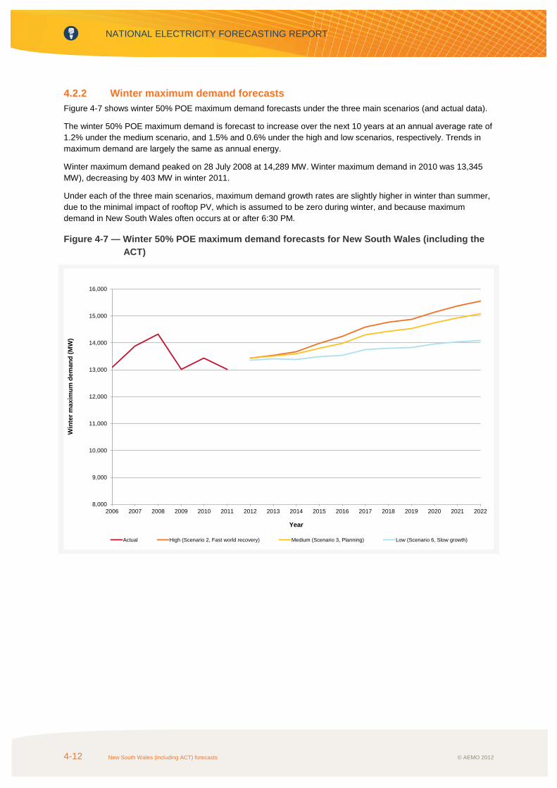
NATIONAL ELECTRICITY FORECASTING REPORT
4-12 New South Wales (including ACT) forecasts © AEMO 2012
4.2.2 Winter maximum demand forecasts Figure 4-7 shows winter 50% POE maximum demand forecasts under the three main scenarios (and actual data).
The winter 50% POE maximum demand is forecast to increase over the next 10 years at an annual average rate of 1.2% under the medium scenario, and 1.5% and 0.6% under the high and low scenarios, respectively. Trends in maximum demand are largely the same as annual energy.
Winter maximum demand peaked on 28 July 2008 at 14,289 MW. Winter maximum demand in 2010 was 13,345 MW), decreasing by 403 MW in winter 2011.
Under each of the three main scenarios, maximum demand growth rates are slightly higher in winter than summer, due to the minimal impact of rooftop PV, which is assumed to be zero during winter, and because maximum demand in New South Wales often occurs at or after 6:30 PM.
Figure 4-7 — Winter 50% POE maximum demand forecasts for New South Wales (including the ACT)
8,000
9,000
10,000
11,000
12,000
13,000
14,000
15,000
16,000
2006 2007 2008 2009 2010 2011 2012 2013 2014 2015 2016 2017 2018 2019 2020 2021 2022
Win
ter m
axim
um d
eman
d (M
W)
Year
Actual High (Scenario 2, Fast world recovery) Medium (Scenario 3, Planning) Low (Scenario 6, Slow growth)

© AEMO 2012 New South Wales (including ACT) forecasts 4-13
Table 4-4 presents actual and forecast winter 10%, 50% and 90% POE maximum demand for New South Wales (including ACT) under the three main scenarios.
Table 4-4 — Winter maximum demand forecasts for New South Wales (including the ACT) (MW)
Actual
High (Scenario 2, Fast World
Recovery) Medium
(Scenario 3, Planning) Low
(Scenario 6, Slow Growth)
10% 50% 90% 10% 50% 90% 10% 50% 90%
2006 13,088 - - - - - - - - -
2007 13,890 - - - - - - - - -
2008 14,316 - - - - - - - - -
2009 13,028 - - - - - - - - -
2010 13,424 - - - - - - - - -
2011 13,030 - - - - - - - - -
2012 - 13,940 13,422 12,988 13,961 13,441 13,007 13,875 13,360 12,926
2013 - 14,042 13,527 13,089 14,032 13,511 13,080 13,919 13,398 12,975
2014 - 14,192 13,667 13,218 14,115 13,581 13,144 13,896 13,377 12,946
2015 - 14,528 13,989 13,528 14,338 13,807 13,353 13,998 13,477 13,033
2016 - 14,793 14,237 13,776 14,539 13,994 13,543 14,066 13,531 13,100
2017 - 15,179 14,577 14,121 14,892 14,290 13,841 14,321 13,739 13,302
2018 - 15,329 14,760 14,273 15,005 14,442 13,967 14,353 13,813 13,357
2019 - 15,453 14,877 14,389 15,112 14,535 14,063 14,367 13,821 13,368
2020 - 15,719 15,132 14,633 15,328 14,743 14,261 14,505 13,951 13,494
2021 - 15,969 15,368 14,855 15,531 14,935 14,447 14,610 14,045 13,582
Average annual growth
- 1.52% 1.52% 1.50% 1.19% 1.18% 1.17% 0.58% 0.56% 0.55%

NATIONAL ELECTRICITY FORECASTING REPORT
4-14 New South Wales (including ACT) forecasts © AEMO 2012
2011 and 2012 forecast comparison
Figure 4-8 compares the 2012 NEFR medium scenario and 2011 ESOO medium economic growth scenario winter 10%, 50% and 90% POE maximum demand forecasts.
The average annual winter 10% POE maximum demand forecast growth rate is expected to be 1.3% over the 10-year outlook period from 2012 to 2021, representing a 0.7% reduction from the 2011 ESOO forecasts.
Figure 4-8 — Comparison of the 2012 NEFR and 2011 ESOO winter maximum demand forecasts for New South Wales (including the ACT)
4.3 Small non-scheduled generation forecasts This section presents forecasts of the contribution from small non-scheduled generation (excluding semi-scheduled, significant non-scheduled, and exempt generation) to annual energy and maximum demand, which are not included in the definition of operational demand.
It is possible that some non-scheduled generators may not be included due to their small size, lack of production, or lack of accurate data. These forecasts consider all non-scheduled generation (as nominated by the jurisdictional planning bodies (JPBs)), which is different from previous reports.
When establishing the adequacy of NEM generation supplies, both the supply-demand outlook and the Medium-term Projected Assessment of System Adequacy (MT PASA) make assessments based only on the demand met by scheduled and semi-scheduled generation, and do not include non-scheduled or exempt generation unless these are considered to have a significant impact on network limitations or the behaviour of other generation.
The small non-scheduled generation forecasts presented in this section are subtracted from both the annual energy and maximum demand forecasts to calculate operational generation forecasts used in the supply-demand outlook.
8,000
10,000
12,000
14,000
16,000
18,000
20,000
2006 2007 2008 2009 2010 2011 2012 2013 2014 2015 2016 2017 2018 2019 2020 2021
Win
ter m
axim
um d
eman
d (M
W)
Year2012 NEFR 10% POE (Medium, Scenario 3, Planning) Actual2011 ESOO 10% POE (Medium) 2012 NEFR 50% POE (Medium, Scenario 3, Planning)2012 NEFR 90% POE (Medium, Scenario 3, Planning) 2011 ESOO 50% POE (Medium)2011 ESOO 90% POE (Medium)

© AEMO 2012 New South Wales (including ACT) forecasts 4-15
For a list of the scheduled and semi-scheduled generators (by region) used to calculate these forecasts, see Appendix C.
Forecasts of small non-scheduled generation energy for New South Wales
Table 4-5 lists the forecast and actual energy of small non-scheduled generation under the three main scenarios.
Table 4-6 presents forecasts of the contribution to summer and winter maximum demand from New South Wales (including ACT) small non-scheduled generation.
Energy supplied by small non-scheduled generating units is forecast to increase over the next 10 years at an annual average rate of between 1.4% and 4.7% (depending on economic scenario), compared with historical annual average growth of 10.4%. Much of the forecast growth can be attributed to the installation of wind, hydro and other renewable sources.
The majority of large projects are expected to register as semi-scheduled rather than non-scheduled. This contributes to relatively low to medium projected growth in non-scheduled energy, capacity, and contribution to summer maximum demand.
Table 4-5 — Forecasts of small non-scheduled generation energy for New South Wales (including ACT) (GWh)
Actual High
(Scenario 2, Fast World Recovery)a
Medium (Scenario 3, Planning)a
Low (Scenario 6,
Slow Growth)a
2005–06 469 - - -
2006–07 469 - - -
2007–08 474 - - -
2008–09 806 - - -
2009–10 806 - - -
2010–11 848 - - -
2011–12 (estimate) 848 - - -
2012–13 - 873 873 873
2013–14 - 899 899 899
2014–15 - 924 924 924
2015–16 - 950 950 950
2016–17 - 975 975 975
2017–18 - 1,000 1,000 1,000
2018–19 - 1,026 1,026 1,026
2019–20 - 1,051 1,051 1,051
2020–21 - 1,077 1,077 1,077
2021–22 - 1,102 1,102 1,102
Average annual growth 10.4% 2.62% 2.62% 2.62%
a. These scenarios assume the same medium (moderate) forecast for small non-scheduled generation.

NATIONAL ELECTRICITY FORECASTING REPORT
4-16 New South Wales (including ACT) forecasts © AEMO 2012
Table 4-6 — Forecasts of the small non-scheduled generation contribution to maximum demand for New South Wales (including ACT) (MW)
Actual
Summer maximum demand
Actual
Winter maximum demand
High (Scenario 2, Fast World Recovery)a
Medium (Scenario
3, Planning)a
Low (Scenario 6, Slow
Growth)a
High (Scenario 2, Fast World Recovery)b
Medium (Scenario
3, Planning)b
Low (Scenario 6,
Slow Growth)b
2005–06 36 - - - - - -
2006–07 20 - - - 13 - - -
2007–08 16 - - - 19 - - -
2008–09 75 - - - 27 - - -
2009–10 75 - - - 15 - - -
2010–11 119 - - - 80 - - -
2011–12 115 - - - 37 - - -
2012–13 - 118 118 118 - 115 115 115
2013–14 - 121 121 121 - 118 118 118
2014–15 - 125 125 125 - 121 121 121
2015–16 - 128 128 128 - 125 125 125
2016–17 - 132 132 132 - 128 128 128
2017–18 - 135 135 135 - 132 132 132
2018–19 - 139 139 139 - 135 135 135
2019–20 - 142 142 142 - 139 139 139
2020–21 - 146 146 146 - 142 142 142
2021–22 - 149 149 149 - 146 146 146
Average annual growth
- 2.62% 2.62% 2.62% - 2.69% 2.69% 2.69%
a. These scenarios assume the same medium (moderate) forecast for small non-scheduled generation.
b. These scenarios assume the same medium (moderate) forecast for small non-scheduled generation.

© AEMO 2012 Queensland forecasts 5-1
CHAPTER 5 - QUEENSLAND FORECASTS
Summary This chapter presents information about annual energy, maximum demand (summer and winter), and non-scheduled generation for the Queensland region. It also includes information about historical annual energy, mass market forecasts, large industrial forecasts, and an annual electrical energy requirement breakdown.
Annual energy
Key differences between the 2012 National Electricity Forecasting Report (NEFR) and Powerlink Queensland’s 2011 annual energy forecasts include the following:
• Annual energy for 2011–12 is expected to be 1.0% lower than 2010–11, and 6.5% lower than forecast in the 2011 Electricity Statement of Opportunities (ESOO) (medium economic growth scenario).
• Forecast annual energy for 2012–13 is expected to only grow by 1.4%, which represents a 10.4% reduction from the 2011 ESOO forecasts.
• Average growth in annual energy for the 10-year outlook period is now forecast to be 2.9%, down from the 4.0% forecast in the 2011 ESOO.
Maximum demand
Key differences between the 2012 NEFR and Powerlink Queensland’s 2011 summer maximum demand medium economic growth scenario forecasts include the following:
• The 2011–12 actual summer maximum demand was 990 MW below Powerlink’s 90% probability of exceedence (POE) forecast.
• AEMO’s 2012–13 summer 10% POE maximum demand forecast is 1,910 MW lower than Powerlink’s 2011 forecast.
• Average growth in 10% POE summer maximum demand for the 10-year outlook period is now forecast to be 2.5%, down from the 4.2% forecast in the 2011 ESOO.
Main factors contributing to forecast change
Annual energy and maximum demand forecasts have decreased since the 2011 ESOO for several main reasons:
• Lower expectation on new project developments from the large industrial sector, including coal seam gas developments and new mining projects forecast to commence from 2013–14.

NATIONAL ELECTRICITY FORECASTING REPORT
5-2 Queensland forecasts © AEMO 2012
• Increasing penetration of rooftop photovoltaics (PV). In 2011–12, rooftop PV systems are estimated to have generated 517 GWh or 1% of estimated annual energy.1 In 2012–13, rooftop PV energy is forecast to be 766 GWh or 1.5% of annual energy under the Planning (medium) scenario. By 2021–22, this is forecast to increase to 2,421 GWh or 3.7% of annual energy. Over the 10-year outlook period, the average annual growth rate of rooftop PV energy is expected to be 13.6%. For more information, see AEMO’s Rooftop PV Information Paper.2
• Reduced manufacturing consumption in response to the high Australian dollar. An expected increase in cheaper imports is expected to partially offset domestic growth.
• A moderation in gross state product (GSP) compared to the 2011 ESOO economic outlook, especially in the short term, influences reduced annual energy forecasts.
• Increasing (real) residential electricity prices. In 2011–12 and 2012–13, electricity prices are expected to increase, and then (on average) moderate from 2013–14 until the end of the outlook period.
• Consumer response (commercial and residential) to rising electricity costs and energy efficiency measures.
• Powerlink uses different maximum demand forecasting methodology.
5.1 Annual energy forecasts This section presents annual energy forecasts for Queensland based on AEMO modelling. For more information about the modelling, see AEMO’s Forecasting Methodology Information Paper.3
Annual energy is defined on a ‘sent-out’ basis. Actual annual energy in 2011–12 includes two financial quarters of actual data and two financial quarters of estimated data.
5.1.1 Annual energy forecasts Annual energy increased on average by 1.8% per year from 2000–01 to 2011–12, underpinned by increasing population and economic growth, higher penetration of air-conditioning units, and increased developments in the industrial sector. Historical annual energy peaked in 2009–10, and has shown negative average annual growth of 1.3% over the last 24 months, with severe weather conditions (floods and cyclones) having an impact.
Annual energy in Queensland is projected to grow over the 10-year outlook period from 2012–13 to 2021–22 at an annual average rate of 2.9% under the medium scenario, and 4.1% and 1.8% under the high and the low scenarios, respectively.
It is expected that in 2012–13 forecasts are similar to actual energy in 2011–12. From 2013–14, changes in the mass market and CSG sector are driving changes in the forecasts.
Annual energy forecasts are offset by the penetration of rooftop PV and energy efficiency savings, which are expected to grow across the 10-year outlook period under all three main scenarios.
1 Estimated annual energy does not include rooftop PV generation. 2 AEMO, available http://www.aemo.com.au/en/Electricity/Forecasting. Viewed June 2012. 3 See note 2.

© AEMO 2012 Queensland forecasts 5-3
Figure 5-1 shows the forecast and actual energy under the three main scenarios. Table 5-1 lists the data used to plot the forecast charts.
Figure 5-1 — Annual energy forecasts for Queensland
37,000
42,000
47,000
52,000
57,000
62,000
67,000
72,000
77,000
Annu
al e
nerg
y (G
wh)
Year
Actual High (Scenario 2, Fast World Recovery) Medium (Scenario 3, Planning) Low (Scenario 6, Slow Growth)

NATIONAL ELECTRICITY FORECASTING REPORT
5-4 Queensland forecasts © AEMO 2012
Table 5-1 — Annual energy forecasts for Queensland (GWh)
Actual High
(Scenario 2, Fast World Recovery)
Medium (Scenario 3, Planning)
Low (Scenario 6, Slow
Growth)
2005-06 47,487
2006–07 48,036 - - -
2007–08 48,313 - - -
2008–09 49,770 - - -
2009–10 50,641 - - -
2010–11 48,862 - - -
2011–12 (estimate) 49,374 - - -
2012–13 - 50,560 50,063 49,590
2013–14 - 53,651 51,873 50,775
2014–15 - 57,682 54,407 52,516
2015–16 - 63,351 58,082 54,943
2016–17 - 66,573 60,383 56,622
2017–18 - 68,583 61,815 57,738
2018–19 - 69,857 62,570 57,860
2019–20 - 70,566 63,157 57,785
2020–21 - 71,728 64,208 58,290
2021–22 - 72,624 64,795 58,465
Average annual growth - 4.1% 2.9% 1.8%

© AEMO 2012 Queensland forecasts 5-5
2011 and 2012 forecast comparison
Over the 9-year outlook period from 2012–13 to 2020–21, there is an average decrease in annual energy of approximately 8,021 GWh from the 2011 ESOO’s medium economic growth scenario forecasts when compared with the 2012 medium scenario forecasts. This is equivalent to a decrease in average annual growth, from 3.9% in the 2011 ESOO to 3.2% in 2012 NEFR.
Figure 5-2 shows actual energy and compares the forecast energy for the two forecasts.
In the near term, 2011–12 annual energy is expected to be 6.5% lower than the 2011 ESOO forecast. From 2011–12 to 2012–13, it is expected to grow by 1.4%, with the annual energy forecast for 2012–13 representing a 10.4% reduction from the 2011 ESOO forecasts.
Figure 5-2 — Comparison of the 2012 NEFR and 2011 ESOO annual energy forecasts for Queensland
40,000
45,000
50,000
55,000
60,000
65,000
70,000
75,000
80,000
Annu
al e
nerg
y (G
wh)
Year
Actual 2011 ESOO (Medium) 2012 NEFR (Medium, Scenario 3, Planning)

NATIONAL ELECTRICITY FORECASTING REPORT
5-6 Queensland forecasts © AEMO 2012
5.1.2 Mass market forecasts Over the 10-year outlook period, the average annual growth rate for the medium, high and low scenarios is expected to be 1.8%, 2.2% and 1.0%, respectively.
Figure 5-3 shows forecast and actual consumption in the mass market sector under the three main scenarios.
Forecasts for the mass market have been calculated by developing a model for non-large industrial consumption, and then subtracting forecasts for rooftop PV and energy efficiency savings. For more information about the model for non-large industrial consumption, see Appendix A.
Figure 5-3 — Mass market forecasts for Queensland
27000
32000
37000
42000
47000
52000
Mas
s M
arke
t ene
rgy
(GW
h)
Year
Actual High (Scenario 2, Fast World Recovery) Medium (Scenario 3, Planning) Low (Scenario 6, Slow Growth)

© AEMO 2012 Queensland forecasts 5-7
5.1.3 Large industrial forecasts Energy consumption in the large industrial sector in Queensland is forecast to increase sharply in the next few years when proposed coal seam gas projects commence operation.
The large industrial forecasts account for a number of new large industrial projects:
• The Xstrata Wandoan coal project.
• Coal seam gas projects in the Bowen and Surat Basins, including:
− Australia Pacific liquefied natural gas (LNG) coal seam gas (CSG) projects – Columbula connections and Orana and North West Surat connections.
− QGC – Kumbarilla Park and Woleebee Creek connections.
− Arrow Energy Surat Gas project.
− Santos Bowen/Surat Basin CSG project.
Although at different stages of project development, all four LNG projects associated with these CSG projects have been approved. Assumptions regarding the scale of these projects vary according to the different scenarios.
AEMO has not included other potential mining and large industrial projects due to the uncertainty that these projects will go ahead.

NATIONAL ELECTRICITY FORECASTING REPORT
5-8 Queensland forecasts © AEMO 2012
Figure 5-4 shows forecast and actual consumption in the large industrial sector for the three main scenarios. Energy consumption is forecast to increase over the next 10 years at an annual average rate of 6.5% under the medium scenario, and 9.6% and 4.7% under the high and low scenarios, respectively.
The difference in these growth rates is primarily due to different assumptions of the scale of LNG projects supported by CSG developments and mining projects in the region. All scenarios assume the 6 committed LNG trains become fully operational by 2017–18.
The low scenario assumes there are no other new large industrial customers commencing operations over the 10 year outlook. Under the medium scenario it is assumed an additional 2,500 GWh, above the low scenario, of large industrial load (equivalent to an additional 3 LNG trains or large mining developments) comes online by 2018–19. Under the high scenario, the majority of the remaining large industrial projects that have commenced feasibility studies are included, which represents an additional 5,500 GWh of large industrial load, by 2018–19, above the medium scenario.
Figure 5-4 — Large industrial forecasts for Queensland
7000
9000
11000
13000
15000
17000
19000
21000
23000
25000
Larg
e In
dust
rial e
nerg
y (G
wh)
Year
Actual High (Scenario 2, Fast World Recovery) Medium (Scenario 3, Planning) Low (Scenario 6, Slow Growth)

© AEMO 2012 Queensland forecasts 5-9
5.1.4 Annual electrical energy requirement breakdown Table 5-2 provides a breakdown of the annual energy forecasts by customer sales, network losses, and auxiliary energy use by generators under the medium scenario.
Table 5-2 — Annual electrical energy requirement breakdown for Queensland (GWh)
Customer sales Transmission network losses
Annual energy (sent out basis)a
Auxiliary energy use
Annual energy (as-generated basis)b
Actual
2005–06 45,947 1,539 47,487 3,891 51,377
2006–07 46,455 1,581 48,036 3,792 51,828
2007–08 46,757 1,557 48,313 3,861 52,174
2008–09 48,266 1,505 49,770 3,947 53,717
2009–10 49,099 1,541 50,641 4,008 54,649
2010–11 47,439 1,423 48,862 3,822 52,684
2011–12 (estimate) 47,743 1,632 49,374 3,760 53,135
Medium scenario (Scenario 3, Planning)
2012–13 48,407 1,656 50,063 3,788 53,851
2013–14 50,152 1,721 51,873 3,896 55,769
2014–15 52,591 1,816 54,407 4,002 58,409
2015–16 56,120 1,962 58,082 4,137 62,220
2016–17 58,325 2,058 60,383 4,232 64,615
2017–18 59,695 2,120 61,815 4,284 66,099
2018–19 60,418 2,153 62,570 4,310 66,880
2019–20 60,979 2,179 63,157 4,337 67,494
2020–21 61,983 2,226 64,208 4,377 68,585
2021–22 62,543 2,252 64,795 4,397 69,192
a. Annual energy (sent out basis) is defined as the total of customer sales and transmission network losses.
b. Annual energy (as-generated basis) is defined as the total of annual energy (sent out basis) and auxiliary energy use.

NATIONAL ELECTRICITY FORECASTING REPORT
5-10 Queensland forecasts © AEMO 2012
5.2 Maximum demand forecasts The maximum demand in Queensland generally occurs in summer.
Half-hourly temperature data was obtained from the Brisbane (Archerfield), Rockhampton and Townsville stations.
5.2.1 Summer maximum demand forecasts Figure 5-5 shows summer 50% POE maximum demand forecasts under the three main scenarios (and actual data).
The summer 50% POE maximum demand is forecast to increase over the next 10 years at an annual average rate of 2.5% under the medium scenario, and 3.4% and 1.5% under the high and low scenarios, respectively. Trends in maximum demand are largely the same as annual energy.
The load factor4 has remained relatively stable, averaging approximately 17.4% during the last 10 years except for 2007–08.
Summer maximum demand peaked on 9 January in 2011–12 at 8,806 MW, decreasing by 102 MW from summer 2010–11.
Figure 5-5 — Summer 50% POE maximum demand forecasts for Queensland
4 The load factor is defined as the annual maximum demand divided by the annual energy.
7,000
8,000
9,000
10,000
11,000
12,000
13,000
Sum
mer
max
imum
dem
and
(MW
)
Year
Actual High (Scenario 2, Fast World Recovery) Medium (Scenario 3, Planning) Low (Scenario 6, Slow Growth)

© AEMO 2012 Queensland forecasts 5-11
Table 5-3 presents actual and forecast summer 10%, 50%, and 90% POE maximum demand for Queensland under the three main scenarios.
Table 5-3 — Summer maximum demand forecasts for Queensland (MW)
Actual
High (Scenario 2, Fast World
Recovery) Medium
(Scenario 3, Planning) Low
(Scenario 6, Slow Growth)
10% 50% 90% 10% 50% 90% 10% 50% 90%
2005–06 8,289 - - - - - - - - -
2006–07 8,664 - - - - - - - - -
2007–08 8,181 - - - - - - - - -
2008–09 8,800 - - - - - - - - -
2009–10 9,061 - - - - - - - - -
2010–11 8,908 - - - - - - - - -
2011–12 8,806 - - - - - - - - -
2012–13 - 9,427 9,129 8,834 9,299 9,007 8,726 9,192 8,904 8,628
2013–14 - 9,896 9,599 9,309 9,558 9,262 8,987 9,355 9,063 8,791
2014–15 - 10,455 10,142 9,844 9,926 9,625 9,334 9,612 9,315 9,038
2015–16 - 11,217 10,895 10,584 10,453 10,142 9,841 9,963 9,659 9,374
2016–17 - 11,650 11,321 11,003 10,785 10,464 10,160 10,218 9,906 9,614
2017–18 - 11,996 11,656 11,326 11,040 10,708 10,396 10,423 10,100 9,801
2018–19 - 12,208 11,860 11,521 11,169 10,830 10,512 10,433 10,099 9,794
2019–20 - 12,339 11,983 11,637 11,285 10,941 10,615 10,417 10,086 9,782
2020–21 - 12,600 12,226 11,872 11,509 11,155 10,817 10,530 10,198 9,887
2021–22 - 12,769 12,388 12,020 11,610 11,245 10,906 10,560 10,217 9,899
Average annual growth
- 3.4% 3.4% 3.5% 2.5% 2.5% 2.5% 1.5% 1.5% 1.5%

NATIONAL ELECTRICITY FORECASTING REPORT
5-12 Queensland forecasts © AEMO 2012
2011 and 2012 forecast comparisons
Figure 5-6 compares the 2012 NEFR medium scenario and 2011 ESOO medium economic growth scenario summer 10%, 50%, and 90% POE maximum demand forecasts.
The average annual summer 10% POE maximum demand forecast growth rate is expected to be 1.6% over the 9-year outlook period from 2012–13 to 2020–21, representing a 0.4% reduction from the 2011 ESOO forecast.
Figure 5-6 — Comparison of the 2012 NEFR and 2011 ESOO summer maximum demand forecasts for Queensland
7,000
8,000
9,000
10,000
11,000
12,000
13,000
14,000
15,000
16,000
Sum
mer
max
imum
dem
and
(MW
)
Year2012 NEFR 10% POE (Medium , Scenario 3, Planning) Actual
2011 ESOO 10% POE (Medium) 2012 NEFR 90% POE (Medium , Scenario 3, Planning)
2012 NEFR 50% POE (Medium , Scenario 3, Planning) 2011 ESOO 90% POE (Medium)
2011 ESOO 50% PE (Medium)
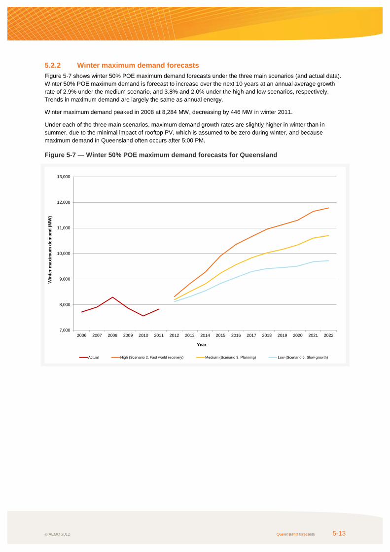
© AEMO 2012 Queensland forecasts 5-13
5.2.2 Winter maximum demand forecasts Figure 5-7 shows winter 50% POE maximum demand forecasts under the three main scenarios (and actual data). Winter 50% POE maximum demand is forecast to increase over the next 10 years at an annual average growth rate of 2.9% under the medium scenario, and 3.8% and 2.0% under the high and low scenarios, respectively. Trends in maximum demand are largely the same as annual energy.
Winter maximum demand peaked in 2008 at 8,284 MW, decreasing by 446 MW in winter 2011.
Under each of the three main scenarios, maximum demand growth rates are slightly higher in winter than in summer, due to the minimal impact of rooftop PV, which is assumed to be zero during winter, and because maximum demand in Queensland often occurs after 5:00 PM.
Figure 5-7 — Winter 50% POE maximum demand forecasts for Queensland
7,000
8,000
9,000
10,000
11,000
12,000
13,000
2006 2007 2008 2009 2010 2011 2012 2013 2014 2015 2016 2017 2018 2019 2020 2021 2022
Win
ter m
axim
um d
eman
d (M
W)
Year
Actual High (Scenario 2, Fast world recovery) Medium (Scenario 3, Planning) Low (Scenario 6, Slow growth)

NATIONAL ELECTRICITY FORECASTING REPORT
5-14 Queensland forecasts © AEMO 2012
Table 5-4 presents actual and forecast winter 10%, 50% and 90% POE maximum demand for Queensland under the three main scenarios.
Table 5-4 — Winter maximum demand forecasts for Queensland (MW)
Actual
High (Scenario 2, Fast World
Recovery) Medium
(Scenario 3, Planning) Low
(Scenario 6, Slow Growth)
10% 50% 90% 10% 50% 90% 10% 50% 90%
2006 7,713 - - - - - - - - -
2007 7,914 - - - - - - - - -
2008 8,284 - - - - - - - - -
2009 7,860 - - - - - - - - -
2010 7,563 - - - - - - - - -
2011 7,838 - - - - - - - - -
2012 - 8,675 8,311 8,085 8,560 8,199 7,974 8,484 8,122 7,901
2013 - 9,182 8,812 8,582 8,880 8,510 8,281 8,678 8,313 8,089
2014 - 9,668 9,278 9,041 9,200 8,818 8,585 8,919 8,548 8,319
2015 - 10,308 9,913 9,667 9,618 9,229 8,987 9,207 8,824 8,590
2016 - 10,758 10,345 10,092 9,964 9,563 9,316 9,443 9,055 8,813
2017 - 11,093 10,670 10,411 10,244 9,830 9,576 9,696 9,296 9,049
2018 - 11,379 10,944 10,674 10,445 10,021 9,759 9,822 9,416 9,169
2019 - 11,574 11,124 10,847 10,598 10,162 9,897 9,850 9,440 9,193
2020 - 11,750 11,295 11,013 10,774 10,331 10,055 9,922 9,507 9,250
2021 - 12,110 11,638 11,345 11,058 10,601 10,318 10,113 9,689 9,433
2022 - 12,258 11,773 11,476 11,158 10,696 10,410 10,138 9,713 9,453
Average annual growth -
3.8% 3.8% 3.8% 2.9% 2.9% 2.9% 2.0% 2.0% 2.0%

© AEMO 2012 Queensland forecasts 5-15
2011 and 2012 forecast comparison
Figure 5-8 compares the 2012 NEFR medium scenario and 2011 ESOO medium economic growth scenario winter 10%, 50% and 90% POE maximum demand forecasts.
The average annual winter 10% POE maximum demand forecast growth rate is expected to be 2.9% over the 10-year outlook period from 2012 to 2021, representing a 1.2% reduction from the 2011 ESOO forecasts.
Figure 5-8 — Comparison of the 2012 NEFR and 2011 ESOO winter maximum demand forecasts for Queensland
7,000
8,000
9,000
10,000
11,000
12,000
13,000
14,000
2006 2007 2008 2009 2010 2011 2012 2013 2014 2015 2016 2017 2018 2019 2020 2021 2022
Win
ter m
axim
um d
eman
d (M
W)
Year2012 NEFR 10% POE (Medium , Scenario 3, Planning) Actual
2011 ESOO 10% POE (Medium) 2012 NEFR 90% POE (Medium , Scenario 3, Planning)
2012 NEFR 50% POE (Medium , Scenario 3, Planning) 2011 ESOO 90% POE (Medium)
2011 ESOO 50% PE (Medium)

NATIONAL ELECTRICITY FORECASTING REPORT
5-16 Queensland forecasts © AEMO 2012
5.3 Small non-scheduled generation forecasts This section presents forecasts of the contribution from small non-scheduled generation (excluding semi-scheduled, significant non-scheduled, and exempt generation) to annual energy and maximum demand, which are not included in the definition of operational demand.
It is possible that some non-scheduled generators may not be included due to their small size, lack of production, or lack of accurate data. These forecasts consider all non-scheduled generation (as nominated by the jurisdictional planning bodies (JPBs)), which is different from previous reports.
When establishing the adequacy of NEM generation supplies, both the supply-demand outlook and Medium-term Projected Assessment of System Adequacy (MT PASA) make assessments based only on the demand met by scheduled and semi-scheduled generation, and do not include non-scheduled or exempt generation unless these are considered to have a significant impact on network limitations or the behaviour of other plants.
The small non-scheduled generation forecasts presented in this section are subtracted from both the annual When establishing the adequacy of NEM generation supplies, both the supply-demand outlook and the MT PASA make assessments based only on the demand met by scheduled and semi-scheduled generation, and do not include non-scheduled or exempt generation unless these are considered to have a significant impact on network limitations or the behaviour of other generation.
The small non-scheduled generation forecasts presented in this section are subtracted from both the annual energy and maximum demand forecasts to calculate operational generation forecasts used in the supply-demand outlook.
For a list of the scheduled and semi-scheduled generators (by region) used to calculate these forecasts, see Appendix C.
Forecasts of small non-scheduled generation energy for Queensland
Table 5-5 lists the forecast and actual energy of small non-scheduled generation under the three main scenarios.
Table 5-6 presents forecasts of the contribution to summer and winter maximum demand from Queensland small non-scheduled generation.
Energy supplied by small non-scheduled generating units in Queensland is forecast to increase over the next 10 years at an annual average rate of between 1.4% and 4.7% (depending on economic scenario), compared with historical annual average growth of 8.6%.
The majority of large projects are expected to register as semi-scheduled rather than non-scheduled. This contributes to relatively low to medium projected growth in non-scheduled energy, capacity, and contribution to summer maximum demand.

© AEMO 2012 Queensland forecasts 5-17
Table 5-5 — Forecasts of small non-scheduled generation energy for Queensland (GWh)
Actual High
(Scenario 2, Fast World Recovery)a
Medium (Scenario 3, Planning)a
Low (Scenario 6, Slow
Growth)a
2005–06 507 - - -
2006–07 628 - - -
2007–08 786 - - -
2008–09 812 - - -
2009–10 834 - - -
2010–11 834 - - -
2011–12 (estimate) 834 - - -
2012–13 - 860 860 860
2013–14 - 885 885 885
2014–15 - 910 910 910
2015–16 - 936 936 936
2016–17 - 961 961 961
2017–18 - 987 987 987
2018–19 - 1,012 1,012 1,012
2019–20 - 1,037 1,037 1,037
2020–21 - 1,063 1,063 1,063
2021–22 - 1,088 1,088 1,088
Average annual growth 8.6% 2.7% 2.7% 2.7%
a. These scenarios assume the same medium (moderate) forecast for small non-scheduled generation.

NATIONAL ELECTRICITY FORECASTING REPORT
5-18 Queensland forecasts © AEMO 2012
Table 5-6 — Forecasts of the small non-scheduled generation contribution to maximum demand for Queensland (MW)
Actual
Summer maximum demand
Actual
Winter maximum demand
High (Scenario 2, Fast World Recovery)a
Medium (Scenario
3, Planning)a
Low (Scenario 6, Slow
Growth)a
High (Scenario 2, Fast World Recovery)b
Medium (Scenario
3, Planning)b
Low (Scenario 6,
Slow Growth)b
2005–06 9 - - - - - -
2006–07 53 - - - 4 - - -
2007–08 95 - - - 52 - - -
2008–09 93 - - - 72 - - -
2009–10 164 - - - 231 - - -
2010–11 82 - - - 225 - - -
2011–12 157 - - - 200 - - -
2012–13 - 163 163 163 - 157 157 157
2013–14 - 169 169 169 - 163 163 163
2014–15 - 175 175 175 - 169 169 169
2015–16 - 181 181 181 - 175 175 175
2016–17 - 187 187 187 - 181 181 181
2017–18 - 193 193 193 - 187 187 187
2018–19 - 199 199 199 - 193 193 193
2019–20 - 205 205 205 - 199 199 199
2020–21 - 211 211 211 - 205 205 205
2021–22 - 217 217 217 - 211 211 211
a. These scenarios assume the same medium (moderate) forecast for small non-scheduled generation.
b. These scenarios assume the same medium (moderate) forecast for small non-scheduled generation.

© AEMO 2012 South Australia forecasts 6-1
CHAPTER 6 - SOUTH AUSTRALIA FORECASTS
Summary This chapter presents information about annual energy, maximum demand (summer and winter), and non-scheduled generation for the South Australian region. It also includes information about historical annual energy, mass market forecasts, large industrial forecasts, and an annual electrical energy requirement breakdown.
Annual energy
Key differences between the 2011 Electricity Statement of Opportunities (ESOO) and the 2012 National Electricity Forecasting Report (NEFR) include the following:
• Annual energy for 2011–12 is expected to be 5.2% lower than 2010–11, and 10.5% lower than forecast in the 2011 ESOO (medium economic growth scenario).
• Forecast annual energy for 2012–13 is expected to only grow by 0.1%, which represents a 12.2% reduction from the 2011 ESOO forecasts.
• Average growth in annual energy for the 10-year outlook period is now forecast to be 0.9%, down from the 1.5% forecast in the 2011 ESOO.
Maximum demand
Key differences between the 2011 ESOO medium economic growth scenario and the 2012 NEFR Planning (medium) scenario summer maximum demand forecasts include the following:
• The 2011–12 actual summer maximum demand was the same as the 2011 ESOO 90% probability of exceedence (POE) forecast.
• The 2012–13 forecast summer 10% POE maximum demand has been reduced by 360 MW.
• Average growth in summer 10% POE maximum demand for the 10-year outlook period is now forecast to be 1.0%, down from the 1.7% forecast in the 2011 ESOO.
Main factors contributing to forecast change
Annual energy and maximum demand forecasts have decreased since the 2011 ESOO for several main reasons:
• A slower than expected forecast increase in consumption from large industrial customers, including developments in the mining sector and the Port Stanvac water desalination plant.
• The significant penetration of rooftop photovoltaics (PV). Among the regions, South Australia has the highest penetration of rooftop PV. In 2011–12, rooftop PV systems are estimated to have generated 306 GWh, or 2.4% of estimated annual energy.1 In 2012–13, rooftop PV energy is forecast to be 448 GWh or 3.4% of annual energy under the Planning (medium) scenario. By 2021–22, this is forecast to increase to 900 GWh or 6.4% of annual energy. Over the 10-year outlook period, the average annual growth rate of rooftop PV energy is expected to be 8.1%. For more information, see AEMO’s Rooftop PV Information Paper.2
• Reduced manufacturing consumption in response to the high Australian dollar. An expected increase in cheaper imports is expected to partially offset domestic growth.
• A moderation in gross state product (GSP) compared to the 2011 ESOO economic outlook, especially in the short term, has influenced reduced annual energy forecasts.
1 Estimated annual energy does not include rooftop PV generation. 2 AEMO, available http://www.aemo.com.au/en/Electricity/Forecasting. Viewed June 2012.
NATIONAL ELECTRICITY FORECASTING REPORT
6-2 South Australia forecasts © AEMO 2012
• Increasing (real) residential electricity prices. In 2011–12 and 2012–13, electricity prices are expected to increase, and then (on average) moderate from 2013–14 until the end of the outlook period.
• Consumer response (commercial and residential) to rising electricity costs and energy efficiency measures.
6.1 Annual energy forecasts This section presents annual energy forecasts for South Australia based on AEMO modelling. For more information about the modelling, see AEMO’s Forecasting Methodology Information Paper.3
Annual energy is defined on a ‘sent-out’ basis. Actual annual energy in 2011–12 includes two financial quarters of actual data and two financial quarters of estimated data.
6.1.1 Annual energy forecasts Annual energy increased on average by 0.5% per year from 2000–01 to 2011–12. Historical annual energy decreased by 3.5% on average from 2000–01 to 2001–02, followed by an increase of 1.6% on average until 2010–11, and a decrease of 5.2% from 2010–11 to 2011–12.
Annual energy in South Australia is projected to grow over the 10-year outlook period from 2012–13 to 2021–22 at an annual average rate of 0.9% under the medium scenario, and 1.6% and 0.03% under the high and the low scenarios, respectively.
It is expected that in 2012–13 forecasts are similar to actual energy in 2011–12. From 2013–14, changes in the mass market and the mining sector are driving changes in the forecasts.
Annual energy forecasts are offset by the penetration of rooftop PV and energy efficiency savings, which are expected to grow across the 10-year outlook period under these three main scenarios.
Figure 6-1 shows the forecast and actual energy under the three main scenarios. Table 6-1 lists the data used to plot the forecast charts.
3 See note 2.

© AEMO 2012 South Australia forecasts 6-3
Figure 6-1 — Annual energy forecasts for South Australia
10,000
11,000
12,000
13,000
14,000
15,000
16,000
17,000
Annu
al e
nerg
y (G
Wh)
Year
Actual High (Scenario 2, Fast world recovery) Medium (Scenario 3, Planning) Low (Scenario 6, Slow growth)

NATIONAL ELECTRICITY FORECASTING REPORT
6-4 South Australia forecasts © AEMO 2012
Table 6-1 — Annual energy forecasts for South Australia (GWh)
Actual High
(Scenario 2, Fast World Recovery)
Medium (Scenario 3, Planning)
Low (Scenario 6, Slow
Growth)
2005–06 12,802 - - -
2006–07 13,451 - - -
2007–08 13,431 - - -
2008–09 13,686 - - -
2009–10 13,621 - - -
2010–11 13,729 - - -
2011–12 (estimate) 13,020 - - -
2012–13 - 13,296 13,031 12,680
2013–14 - 13,783 13,226 12,659
2014–15 - 14,068 13,418 12,616
2015–16 - 14,275 13,440 12,556
2016–17 - 14,632 13,572 12,535
2017–18 - 14,703 13,637 12,563
2018–19 - 14,950 13,843 12,619
2019–20 - 15,073 13,947 12,659
2020–21 - 15,254 14,108 12,755
2021–22 - 15,290 14,123 12,713
Average annual growth - 1.56% 0.90% 0.03%

© AEMO 2012 South Australia forecasts 6-5
2011 and 2012 forecast comparison
Over the 9-year outlook period from 2012–13 to 2020–21, there is an average decrease in annual energy of approximately 2,180 GWh from the 2011 ESOO’s medium economic growth scenario forecasts when compared with the 2012 medium scenario forecasts. This is equivalent to a decrease in average annual growth, from 1.5% in the 2011 ESOO to 0.9% in the 2012 NEFR.
Figure 6-2 shows actual energy and compares the forecast energy for the two forecasts.
In the near term, 2011–12 annual energy is expected to be 10.5% lower than the 2011 ESOO forecast. From 2011–12 to 2012–13, it is expected to remain flat, with the annual energy forecast for 2012–13 representing a 12.2% reduction from the 2011 ESOO forecast.
Figure 6-2 — Comparison of the 2012 NEFR and 2011 ESOO annual energy forecasts for South Australia
10,000
11,000
12,000
13,000
14,000
15,000
16,000
17,000
18,000
Annu
al e
nerg
y (G
Wh)
Year
Actual 2012 NEFR (Medium, Scenario 3, Planning) 2011 ESOO (Medium)

NATIONAL ELECTRICITY FORECASTING REPORT
6-6 South Australia forecasts © AEMO 2012
6.1.2 Mass market forecasts Over the 10-year outlook period, the average annual growth rate for the medium, high and low scenarios is expected to be 0.5%, 0.7% and 0.1%, respectively.
Figure 6-3 shows forecast and actual consumption in the mass market under the three main scenarios.
Forecasts for the mass market have been calculated by developing a model for non-large industrial consumption, and then subtracting forecasts for rooftop PV and energy efficiency savings. For more information about the model for non-large industrial consumption, see Appendix A.
Figure 6-3 — Mass market forecasts for South Australia
9,000
9,500
10,000
10,500
11,000
11,500
12,000
12,500
13,000
Mas
s m
arke
t ene
rgy
(GW
h)
Year
Actual High (Scenario 2, Fast world recovery) Medium (Scenario 3, Planning) Low (Scenario 6, Slow growth)

© AEMO 2012 South Australia forecasts 6-7
6.1.3 Large industrial forecasts The large industrial forecasts include a number of new and existing customers:
• DSC Woomera.
• SANTOS Stony Point.
• SA Water (including the seawater desalination pumping stations).
• AMCOR Roseworthy.
• BHP Billiton (Olympic Dam).
• One Steel Middleback.
• Alinta Energy Leigh Creek Coal-field.
• Kimberly Clark.
New planning proposals for future large industrial projects (requiring transmission network connection points) and further mining exploration activity may potentially be developed in South Australia, but are not accounted for by the scenarios, due to a lack of sufficient information.
Figure 6-4 shows forecast and actual consumption in the large industrial sector under the three main scenarios. Energy consumption is forecast to increase over the next 10 years at an annual average rate of 2.8% under the medium scenario, and 5.2% and 0.4% under the high and low scenarios, respectively.
Figure 6-4 — Large industrial forecasts for South Australia
0
500
1,000
1,500
2,000
2,500
3,000
3,500
4,000
Larg
e in
dust
rial e
nerg
y (G
Wh)
Year
Actual High (Scenario 2, Fast world recovery) Medium (Scenario 3, Planning) Low (Scenario 6, Slow growth)

NATIONAL ELECTRICITY FORECASTING REPORT
6-8 South Australia forecasts © AEMO 2012
6.1.4 Annual electrical energy requirement breakdown Table 6-2 provides a breakdown of the annual energy forecasts by customer sales, network losses, and auxiliary energy use by generators under the medium scenario.
Table 6-2 — Annual electrical energy requirement breakdown for South Australia (GWh)
Customer sales Transmission network losses
Annual energy (sent out basis)a
Auxiliary energy use
Annual energy (as-generated basis)b
Actual
2005–06 12,509 293 12,802 876 13,678
2006–07 13,174 277 13,451 773 14,224
2007–08 13,183 247 13,431 840 14,271
2008–09 13,386 296 13,686 807 14,493
2009–10 13,291 313 13,621 780 14,401
2010–11 13,376 311 13,729 769 14,498
2011–12 (estimate) 12,774 246 13,020 725 13,745
Medium scenario (Scenario 3, Planning)
2012–13 12,785 246 13,031 714 13,745
2013–14 12,973 254 13,226 721 13,947
2014–15 13,158 261 13,418 727 14,145
2015–16 13,178 262 13,440 727 14,166
2016–17 13,305 267 13,572 730 14,302
2017–18 13,368 269 13,637 735 14,373
2018–19 13,565 277 13,843 741 14,584
2019–20 13,666 281 13,947 749 14,696
2020–21 13,820 288 14,108 753 14,861
2021–22 13,834 288 14,123 754 14,877
a. Annual energy (sent out basis) is defined as the total of customer sales and transmission network losses.
b. Annual energy (as-generated basis) is defined as the total of annual energy (sent out basis) and auxiliary energy use.

© AEMO 2012 South Australia forecasts 6-9
6.2 Maximum demand forecasts The maximum demand in South Australia occurs in summer.
Half-hourly temperature data was obtained from the Kent Town station.
6.2.1 Summer maximum demand forecasts Figure 6-5 shows summer 50% POE maximum demand forecasts under the three main scenarios (and actual data).
The summer 50% POE maximum demand is forecast to increase over the next 10 years at an annual average rate of 1% under the medium scenario, and 1.4% and 0.3% under the high and low scenarios, respectively. Trends in maximum demand are largely the same as annual energy.
The load factor4 for summer has averaged approximately 23% during the last 10 years.
Summer maximum demand peaked on 31 January in 2010–11 at 3,423 MW, decreasing by 445 MW in summer 2011–12.
Figure 6-5 — Summer 50% POE maximum demand forecasts for South Australia
4 The load factor is defined as the annual maximum demand divided by the annual energy.
1,800
2,200
2,600
3,000
3,400
3,800
4,200
Sum
mer
max
imum
dem
and
(MW
)
Year
Actual High (Scenario 2, Fast world recovery) Medium (Scenario 3, Planning) Low (Scenario 6, Slow growth)

NATIONAL ELECTRICITY FORECASTING REPORT
6-10 South Australia forecasts © AEMO 2012
Table 6-3 presents actual and forecast summer 10%, 50%, and 90% POE maximum demand for South Australia under the three main scenarios.
Table 6-3 — Summer maximum demand forecasts for South Australia (MW)
Actual
High (Scenario 2, Fast World
Recovery) Medium
(Scenario 3, Planning) Low
(Scenario 6, Slow Growth)
10% 50% 90% 10% 50% 90% 10% 50% 90%
2005–06 2,935 - - - - - - - - -
2006–07 2,936 - - - - - - - - -
2007–08 3,173 - - - - - - - - -
2008–09 3,401 - - - - - - - - -
2009–10 3,309 - - - - - - - - -
2010–11 3,424 - - - - - - - - -
2011–12 2,979 - - - - - - - - -
2012–13 - 3,308 3,025 2,811 3,271 2,990 2,778 3,218 2,939 2,728
2013–14 - 3,410 3,118 2,901 3,332 3,045 2,826 3,247 2,963 2,747
2014–15 - 3,455 3,163 2,943 3,362 3,073 2,855 3,242 2,957 2,742
2015–16 - 3,496 3,201 2,976 3,375 3,083 2,861 3,236 2,950 2,734
2016–17 - 3,558 3,259 3,031 3,407 3,112 2,887 3,245 2,956 2,737
2017–18 - 3,591 3,287 3,056 3,439 3,140 2,911 3,268 2,975 2,752
2018–19 - 3,646 3,335 3,100 3,488 3,183 2,951 3,288 2,992 2,766
2019–20 - 3,682 3,367 3,128 3,521 3,211 2,974 3,305 3,005 2,777
2020–21 - 3,740 3,417 3,173 3,573 3,256 3,015 3,340 3,036 2,804
2021–22 - 3,750 3,425 3,177 3,578 3,259 3,015 3,332 3,026 2,792
Average annual growth
- 1.4% 1.4% 1.4% 1.0% 1.0% 0.9% 0.39% 0.33% 0.26%

© AEMO 2012 South Australia forecasts 6-11
2011 and 2012 forecast comparison
Figure 6-6 compares the 2012 NEFR medium scenario and 2011 ESOO medium economic growth scenario summer 10%, 50%, and 90% POE maximum demand forecasts.
The average annual summer 10% POE maximum demand forecast growth rate is expected to be 1.1% over the 9-year outlook period from 2012–13 to 2020–21, representing a 0.6% reduction from the 2011 ESOO forecast.
Figure 6-6 — Comparison of the 2012 NEFR and 2011 ESOO summer maximum demand forecasts for South Australia
2,000
2,300
2,600
2,900
3,200
3,500
3,800
4,100
4,400
4,700
Sum
mer
max
imum
dem
and
(MW
)
Year2012 NEFR 10% POE (Medium, Scenario 3, Planning) Actual
2011 ESOO 10% POE (Medium) 2012 NEFR 90% POE (Medium, Scenario 3, Planning)
2012 NEFR 50% POE (Medium, Scenario 3, Planning) 2011 ESOO 90% POE (Medium)
2011 ESOO 50% POE (Medium)

NATIONAL ELECTRICITY FORECASTING REPORT
6-12 South Australia forecasts © AEMO 2012
6.2.2 Winter maximum demand forecasts Figure 6-7 shows winter 50% POE maximum demand forecasts under the three main scenarios (and actual data).
The winter 50% POE maximum demand is forecast to increase over the next 10 years at an annual average rate of 1.2% under the medium scenario, and 1.8% and 0.4% under the high and low scenarios, respectively. Trends in maximum demand are largely the same as annual energy.
Winter maximum demand peaked on 29 July 2008 at 2,530 MW (and was only slightly lower in 2010 at 2,523 MW), decreasing by 143 MW in winter 2011.
The impact of rooftop PV on winter maximum demand is assumed to be zero due to the maximum demand in South Australia often occurring in the evening around 6:30 PM to 7:30 PM, coinciding with increased use of space heating and electrical appliances.
Figure 6-7 — Winter 50% POE maximum demand forecasts for South Australia
1,800
2,000
2,200
2,400
2,600
2,800
3,000
3,200
3,400
2006 2007 2008 2009 2010 2011 2012 2013 2014 2015 2016 2017 2018 2019 2020 2021
Win
ter m
axim
um d
eman
d (M
W)
Year
Actual High (Scenario 2, Fast world recovery) Medium (Scenario 3, Planning) Low (Scenario 6, Slow growth)

© AEMO 2012 South Australia forecasts 6-13
Table 6-4 lists actual and forecast winter 10%, 50%, and 90% POE maximum demand for South Australia under the three main scenarios.
Table 6-4 — Winter maximum demand forecasts for South Australia (MW)
Actual
High (Scenario 2, Fast World
Recovery) Medium
(Scenario 3, Planning) Low
(Scenario 6, Slow Growth)
10% 50% 90% 10% 50% 90% 10% 50% 90%
2006 2,379 - - - - - - - - -
2007 2,458 - - - - - - - - -
2008 2,530 - - - - - - - - -
2009 2,445 - - - - - - - - -
2010 2,523 - - - - - - - - -
2011 2,380 - - - - - - - - -
2012 - 2,578 2,476 2,412 2,574 2,472 2,408 2,565 2,462 2,398
2013 - 2,623 2,513 2,447 2,596 2,487 2,421 2,561 2,452 2,387
2014 - 2,690 2,578 2,511 2,627 2,516 2,450 2,556 2,445 2,380
2015 - 2,743 2,629 2,562 2,653 2,542 2,475 2,552 2,442 2,377
2016 - 2,789 2,676 2,607 2,682 2,571 2,505 2,557 2,447 2,381
2017 - 2,836 2,719 2,649 2,705 2,591 2,523 2,563 2,451 2,385
2018 - 2,894 2,778 2,708 2,748 2,636 2,567 2,594 2,484 2,417
2019 - 2,937 2,819 2,748 2,788 2,674 2,603 2,615 2,503 2,436
2020 - 2,987 2,869 2,796 2,833 2,717 2,645 2,642 2,530 2,461
2021 - 3,026 2,902 2,828 2,869 2,747 2,675 2,667 2,548 2,479
Average annual growth
- 0.43% 0.38% 0.37% 1.21% 1.18% 1.17% 1.80% 1.78% 1.79%

NATIONAL ELECTRICITY FORECASTING REPORT
6-14 South Australia forecasts © AEMO 2012
2011 and 2012 forecast comparison
Figure 6-8 the 2012 NEFR medium scenario and 2011 ESOO medium economic growth winter 10%, 50%, and 90% POE maximum demand forecasts.
The average annual winter 10% POE maximum demand forecast growth rate is expected to be 1.2% over the 10-year outlook period from 2012 to 2021, representing a 0.4% reduction from the 2011 ESOO forecasts.
Figure 6-8 — Comparison of the 2012 NEFR and 2011 ESOO forecasts for South Australia
6.3 Small non-scheduled generation forecasts This section presents forecasts of the contribution from small non-scheduled generation (excluding semi-scheduled, significant non-scheduled, and exempt generation) to annual energy and maximum demand, which are not included in the definition of operational demand.
It is possible that some non-scheduled generators may not be included due to their small size, lack of production, or lack of accurate data. These forecasts consider all non-scheduled generation (as nominated by the jurisdictional planning bodies (JPBs)), which is different from previous reports.
When establishing the adequacy of NEM generation supplies, both the supply-demand outlook and the Medium-term Projected Assessment of System Adequacy (MT PASA) make assessments based only on the demand met by scheduled and semi-scheduled generation, and do not include non-scheduled or exempt generation unless these are considered to have a significant impact on network limitations or the behaviour of other generation.
The small non-scheduled generation forecasts presented in this section are subtracted from both the annual energy and maximum demand forecasts to calculate operational generation forecasts used in the supply-demand outlook.
1,800
2,000
2,200
2,400
2,600
2,800
3,000
3,200
3,400
3,600
2006 2007 2008 2009 2010 2011 2012 2013 2014 2015 2016 2017 2018 2019 2020 2021
Win
ter m
axim
um d
eman
d (M
W)
Year2012 NEFR 10% POE (Medium, Scenario 3, Planning) Actual2011 ESOO 10% POE (Medium) 2012 NEFR 90% POE (Medium, Scenario 3, Planning)2012 NEFR 50% POE (Medium, Scenario 3, Planning) 2011 ESOO 90% POE (Medium)2011 ESOO 50% POE (Medium)

© AEMO 2012 South Australia forecasts 6-15
For a list of the scheduled and semi-scheduled generators (by region) used to calculate these forecasts, see Appendix C.
Forecasts of small non-scheduled generation energy for South Australia
Table 6-5 lists the forecast and actual energy of small non-scheduled generation under the three main scenarios.
Table 6-6 presents forecasts of the contribution to summer and winter maximum demand from South Australian small non-scheduled generation.
Energy supplied by small non-scheduled generating units in South Australia is forecast to increase over the next 10 years at an annual average rate of between 9.1% and 17.9% (depending on economic scenario), compared with historical annual average growth of 38%.
The majority of large projects are expected to register as semi-scheduled rather than non-scheduled. This contributes to relatively low to medium projected growth in non-scheduled energy, capacity, and contribution to summer maximum demand.
Table 6-5 — Forecasts of small non-scheduled generation energy for South Australia (GWh)
Actual energy High
(Scenario 2, Fast World Recovery)a
Medium (Scenario 3, Planning)a
Low (Scenario 6, Slow
Growth)a
2005–06 10 - - -
2006–07 10 - - -
2007–08 10 - - -
2008–09 10 - - -
2009–10 10 - - -
2010–11 10 - - -
2011–12 (estimate) 69 - - -
2012–13 - 90 90 90
2013–14 - 111 111 111
2014–15 - 133 133 133
2015–16 - 154 154 154
2016–17 - 175 175 175
2017–18 - 196 196 196
2018–19 - 217 217 217
2019–20 - 238 238 238
2020–21 - 260 260 260
2021–22 - 281 281 281
Average annual growth 32.1% 12.5% 12.5% 12.5%
a. These scenarios assume the same medium (moderate) forecast for small non-scheduled generation.

NATIONAL ELECTRICITY FORECASTING REPORT
6-16 South Australia forecasts © AEMO 2012
Table 6-6 — Forecasts of the small non-scheduled generation contribution to maximum demand for South Australia (MW)
Actual
Maximum demand
Scenario 1 Fast Rate of Change
Scenario 2 Fast World Recovery
Scenario 3 Planning
Scenario 4 Decentralised
World
Scenario 5 Slow Rate of Change
Scenario 6 Slow
Growth
2005-06 19 2006-07 21 2007-08 21 2008-09 17 2009-10 1 2010-11 25 2011-12 21 2012-13 22 22 22 22 22 22 2013-14 23 23 23 23 23 23 2014-15 24 24 24 24 24 24 2015-16 26 26 26 26 26 26 2016-17 27 27 27 27 27 27 2017-18 28 28 28 28 28 28 2018-19 29 29 29 29 29 29 2019-20 30 30 30 30 30 30 2020-21 31 31 31 31 31 31 2021-22 32 32 32 32 32 32 2022-23 34 34 34 34 34 34 2023-24 35 35 35 35 35 35 2024-25 36 36 36 36 36 36 2025-26 37 37 37 37 37 37 2026-27 38 38 38 38 38 38 2027-28 39 39 39 39 39 39 2028-29 40 40 40 40 40 40 2029-30 42 42 42 42 42 42 2030-31 43 43 43 43 43 43 2031-32 44 44 44 44 44 44
a. These scenarios assume the same medium (moderate) forecast for small non-scheduled generation.
b. These scenarios assume the same medium (moderate) forecast for small non-scheduled generation.

© AEMO 2012 Tasmania forecasts 7-1
CHAPTER 7 - TASMANIA FORECASTS
Summary This chapter presents information about annual energy, maximum demand (summer and winter), and non-scheduled generation for the Tasmanian region. It also includes information about historical annual energy, mass market forecasts, large industrial forecasts, and an annual electrical energy requirement breakdown.
Annual energy
Key differences between the 2012 National Electricity Forecasting Report (NEFR) and Transend Network’s 2011 annual energy forecasts, published in the 2011 ESOO, include the following:
• Annual energy for 2011-12 is expected to be 5.0% lower than 2010-11 and 7.3% lower than what was forecast in the 2011 ESOO (medium economic growth scenario).
• Forecast annual energy for 2012-13 is expected to increase by 0.7%, which represents an 8.5% reduction from the 2011 ESOO forecasts.
• Average growth in annual energy for the 10-year outlook period is forecast to be 0.9%, the same as was forecast in the 2011 ESOO.
Maximum demand
Key differences between the 2012 NEFR and Transend Network’s 2011 winter maximum demand medium economic growth scenario forecasts include the following:
• The 2011 actual winter maximum demand was 40 MW below Transend Network’s 90% POE forecast.
• The 2012 forecast winter 10% POE maximum demand is 110 MW lower than Transend’s 2011 forecast.
• Average growth in winter 10% POE maximum demand for the 10-year outlook period is now forecast to be 1.1%, down from the 1.4% forecast in the 2011 ESOO.
• AEMO and Transend use different maximum demand forecasting methodology.
Main factors contributing to forecast change
Annual energy and maximum demand forecasts have decreased since the 2011 ESOO for several main reasons:
• Reduced consumption from large industrial customers. In 2011–12, energy use is expected to decline mainly due to BHP’s Tasmanian Electro Metallurgical Company (TEMCO) manganese smelter suspending production between March and May 2012. In May 2012, BHP announced that TEMCO operations will be restarted and resume operating at full capacity by the end of August 2012.
• Increasing penetration of rooftop photovoltaics (PV). In 2011–12, rooftop PV systems are estimated to have generated 15 GWh or 0.1% of estimated annual energy.1 In 2012–13, rooftop PV energy is forecast to be 30 GWh or 0.3% of annual energy under the Planning (medium) scenario. By 2021–22, this is forecast to increase to 147 GWh or 1.3% of annual energy. Over the 10-year outlook period, the average annual growth rate of rooftop PV energy is expected to be 19.3%. For more information, see AEMO’s Rooftop PV Information Paper.2
• Reduced manufacturing consumption in response to the high Australian dollar. An expected increase in cheaper imports is expected to partially offset domestic growth.
1 Estimated annual energy does not include rooftop PV generation. 2 AEMO, available http://www.aemo.com.au/en/Electricity/Forecasting. Viewed June 2012.

NATIONAL ELECTRICITY FORECASTING REPORT
7-2 Tasmania forecasts © AEMO 2012
• A decrease in economic growth (measured by gross state product (GSP)) forecasts since the 2011 ESOO influences lower energy forecasts, particularly in the short term.
• Increasing (real) residential electricity prices. In 2011–12 and 2012–13, electricity prices are expected to increase, and then (on average) moderate from 2013–14 until the end of the outlook period.
• Consumer response (commercial and residential) to rising electricity costs and energy efficiency measures.
7.1 Annual energy forecasts This section presents annual energy forecasts for Tasmania based on AEMO modelling. For more information about the modelling, see AEMO’s Forecasting Methodology Information Paper.3
Annual energy is defined on a ‘sent-out’ basis. Actual annual energy in 2011–12 includes two financial quarters of actual data and two financial quarters of estimated data.
7.1.1 Annual energy forecasts Annual energy increased on average by 0.7% per year from 2002–03 to 2011–12. Historical annual energy peaked in 2007–08 and 2008–09, followed by largely negative annual average growth until 2011–12. In 2010–11, there was a brief recovery in economic growth, cooler winter conditions, and an increase in energy use in the industrial sector.
Annual energy in Tasmania is projected to grow over the 10-year outlook period from 2012–13 to 2021–22 at an annual average rate of 0.9% under the medium scenario, and 1.7% and -0.02% under the high and the low scenarios, respectively.
It is expected that in 2012–13 forecasts are similar to actual energy in 2011–12. From 2013–14, changes in the large industrial sector (smelting and mining) are driving changes in the forecasts.
Annual energy forecasts are offset by the penetration of rooftop PV and energy efficiency savings, which are expected to grow across the 10-year outlook period under these three main scenarios.
3 See note 2.

© AEMO 2012 Tasmania forecasts 7-3
Figure 7-1 shows the forecast and actual energy for the three main scenarios.
Table 7-1 lists the data used to plot the forecast charts.
Figure 7-1 — Annual energy forecasts for Tasmania
0
2,000
4,000
6,000
8,000
10,000
12,000
14,000
Annu
al e
nerg
y (G
Wh)
Year
Actual High (Scenario 2, Fast world recovery) Medium (Scenario 3, Planning) Low (Scenario 6, Slow growth)

NATIONAL ELECTRICITY FORECASTING REPORT
7-4 Tasmania forecasts © AEMO 2012
Table 7-1 — Annual energy forecasts for Tasmania (GWh)
Actual High
(Scenario 2, Fast World Recovery)
Medium (Scenario 3, Planning)
Low (Scenario 6,
Slow Growth)
2005–06 10,574 - - -
2006–07 10,667 - - -
2007–08 10,974 - - -
2008–09 10,979 - - -
2009–10 10,877 - - -
2010–11 10,934 - - -
2011–12 (estimate) 10,391 - - -
2012–13 - 10,681 10,466 9,666
2013–14 - 10,778 10,494 9,451
2014–15 - 10,930 10,578 9,291
2015–16 - 11,050 10,716 9,239
2016–17 - 11,507 10,877 9,346
2017–18 - 11,835 10,959 9,404
2018–19 - 12,104 10,988 9,414
2019–20 - 12,091 11,044 9,438
2020–21 - 12,205 11,169 9,520
2021–22 - 12,419 11,336 9,652
Average annual growth - 1.69% 0.89% -0.02%

© AEMO 2012 Tasmania forecasts 7-5
2011 and 2012 forecast comparison
Over the 9-year outlook period from 2012–13 to 2020–21, there is an average reduction of 947 GWh from the 2011 ESOO’s medium economic growth scenario forecasts when compared with the 2012 medium scenario forecasts. This is equivalent to average annual growth of 0.9% for both the 2011 ESOO and the 2012 NEFR.
Figure 7-2 shows actual energy and compares the forecast energy for the two forecasts.
In the near term, 2011–12 annual energy was 7.3% lower than the 2011 ESOO forecast. From 2011–12 to 2012–13, it is expected to grow by 0.7%, with the annual energy forecast for 2012–13 representing an 8.5% reduction from the 2011 ESOO forecasts.
Figure 7-2 — Comparison of the 2012 NEFR and 2011 ESOO annual energy forecasts for Tasmania
8,500
9,000
9,500
10,000
10,500
11,000
11,500
12,000
12,500
13,000
Annu
al e
nerg
y (G
Wh)
Year
Actual 2012 NEFR (Medium, Scenario 3, Planning) ESOO 2011 (Medium)

NATIONAL ELECTRICITY FORECASTING REPORT
7-6 Tasmania forecasts © AEMO 2012
7.1.2 Mass market forecasts Over the 10-year outlook period, the average annual growth rate for the medium, high and low scenarios is expected to be 1.1%, 1.1% and 0.7%, respectively.
There is only a small difference between the medium and high scenarios, which is due to stronger economic growth and higher electricity prices offsetting each other under the high scenario.
Figure 7-3 shows forecast and actual consumption in the mass market sector under the three main scenarios.
Forecasts for the mass market have been calculated by developing a model for non-large industrial consumption, and then subtracting forecasts for rooftop PV and energy efficiency savings. For more information about the model for non-large industrial consumption, see Appendix A.
Figure 7-3 — Mass market forecasts for Tasmania
4,200
4,400
4,600
4,800
5,000
5,200
5,400
5,600
Mas
s m
arke
t ene
rgy
(GW
h)
Year
Actual High (Scenario 2, Fast world recovery) Medium (Scenario 3, Planning) Low (Scenario 6, Slow growth)

© AEMO 2012 Tasmania forecasts 7-7
7.1.3 Large industrial forecasts The large industrial forecasts account for a number of new and existing projects:
• BHP’s TEMCO manganese smelter suspended production between March and May 2012, with operations to resume at full capacity by the end of August 2012.4
• Gunn’s Pulp Mill at Bell Bay, which contributes significantly to growth under the high scenario.
• Weakness in the metals sector, which slows growth under the low scenario.
Figure 7-4 shows forecast and actual consumption in the large industrial sector for the three main scenarios. Energy consumption is forecast to increase over the next 10 years at an annual average rate of 0.7% under the medium scenario, and 2.1% and -0.7% under the high and low scenarios, respectively.
Figure 7-4 — Large industrial forecasts for Tasmania
4 See note 5.
0
1,000
2,000
3,000
4,000
5,000
6,000
7,000
8,000
Larg
e in
dust
rial e
nerg
y (G
Wh)
Year
Actual High (Scenario 2, Fast world recovery) Medium (Scenario 3, Planning) Low (Scenario 6, Slow growth)

NATIONAL ELECTRICITY FORECASTING REPORT
7-8 Tasmania forecasts © AEMO 2012
7.1.4 Annual electrical energy requirement breakdown Table 7-2 provides a breakdown of the annual energy forecasts by customer sales, network losses, and auxiliary energy use by generators under the medium scenario.
Table 7-2 — Annual electrical energy requirement breakdown for Tasmania (GWh)
Customer sales
Transmission network losses
Annual energy (sent out basis)a
Auxiliary energy use
Annual energy (as-generated basis)b
Actual
2005–06 10,293 281 10,574 65 10,639
2006–07 10,431 236 10,667 121 10,788
2007–08 10,722 252 10,974 117 11,091
2008–09 10,711 268 10,979 58 11,037
2009–10 10,572 304 10,877 73 10,950
2010–11 10,631 304 10,934 126 11,060
2011–12 (estimate) 10,142 249 10,391 78 10,469
Scenario 3 - Planning
2012–13 10,213 252 10,466 78 10,543
2013–14 10,240 254 10,494 78 10,572
2014–15 10,320 258 10,578 78 10,656
2015–16 10,452 264 10,716 78 10,795
2016–17 10,605 272 10,877 79 10,956
2017–18 10,683 276 10,959 79 11,038
2018–19 10,711 278 10,988 79 11,067
2019–20 10,763 280 11,044 79 11,123
2020–21 10,882 287 11,169 79 11,248
2021–22 11,041 295 11,336 80 11,415
a. Annual energy (sent out basis) is defined as the total of customer sales and transmission network losses.
b. Annual energy (as-generated basis) is defined as the total of annual energy (sent out basis) and auxiliary energy use.

© AEMO 2012 Tasmania forecasts 7-9
7.2 Maximum demand forecasts The maximum demand in Tasmania occurs in winter.
Half-hourly temperature data was obtained from Hobart’s Ellerslie Road station.
7.2.1 Summer maximum demand forecasts Figure 7-5 shows summer 50% POE maximum demand forecasts under the three main scenarios (and actual data).
The summer 50% POE maximum demand is forecast to increase over the next 10 years at an annual average rate of 1.1% under the medium scenario, and 1.8% and 0.3% under the high and low scenarios, respectively. Trends in maximum demand are largely the same as annual energy.
Figure 7-5 — Summer 50% POE maximum demand forecasts for Tasmania
0
200
400
600
800
1,000
1,200
1,400
1,600
1,800
Sum
mer
max
imum
dem
and
(MW
)
Year
Actual High (Scenario 2, Fast world recovery) Medium (Scenario 3, Planning) Low (Scenario 6, Slow growth)

NATIONAL ELECTRICITY FORECASTING REPORT
7-10 Tasmania forecasts © AEMO 2012
Table 7-3 presents actual and forecast summer 10%, 50% and 90% POE maximum demand for Tasmania under the three main scenarios.
Table 7-3 — Summer maximum demand forecasts for Tasmania (MW)
Actual
High Medium Low
(Scenario 2, Fast World Recovery) (Scenario 3, Planning) (Scenario 6, Slow Growth)
10% 50% 90% 10% 50% 90% 10% 50% 90%
2005–06 1,311 - - - - - - - - -
2006–07 1,401 - - - - - - - - -
2007–08 1,438 - - - - - - - - -
2008–09 1,487 - - - - - - - - -
2009–10 1,400 - - - - - - - - -
2010–11 1,392 - - - - - - - - -
2011–12 1,423 - - - - - - - - -
2012–13 - 1,437 1,397 1,365 1,412 1,371 1,339 1,317 1,277 1,245
2013–14 - 1,454 1,414 1,380 1,420 1,381 1,347 1,298 1,259 1,225
2014–15 - 1,478 1,437 1,402 1,436 1,395 1,360 1,283 1,243 1,210
2015–16 - 1,498 1,456 1,421 1,459 1,417 1,382 1,283 1,242 1,209
2016–17 - 1,557 1,514 1,478 1,483 1,440 1,405 1,301 1,260 1,225
2017–18 - 1,601 1,557 1,520 1,498 1,455 1,418 1,313 1,271 1,236
2018–19 - 1,636 1,591 1,554 1,505 1,461 1,425 1,317 1,275 1,239
2019–20 - 1,637 1,593 1,556 1,516 1,472 1,435 1,322 1,280 1,245
2020–21 - 1,657 1,612 1,573 1,536 1,492 1,453 1,336 1,294 1,257
2021–22 - 1,688 1,643 1,603 1,561 1,516 1,477 1,358 1,315 1,278
Average annual growth - 1.80% 1.82% 1.81% 1.13% 1.12% 1.10% 0.34% 0.32% 0.29%
2011 and 2012 forecast comparison
Figure 7-6 compares the 2012 NEFR medium scenario and 2011 ESOO medium economic growth scenario summer 10%, 50% and 90% POE maximum demand forecasts.
The average annual summer 10% POE maximum demand forecast growth rate is expected to be 1.1% over the 9-year outlook period from 2012–13 to 2020–21, representing a 0.3% reduction from the 2011 ESOO forecasts.

© AEMO 2012 Tasmania forecasts 7-11
Figure 7-6 — Comparison of the 2012 NEFR and 2011 ESOO summer maximum demand forecasts for Tasmania
800
900
1,000
1,100
1,200
1,300
1,400
1,500
1,600
1,700
1,800
Sum
mer
max
imum
dem
and
(WM
)
Year2012 NEFR 10% POE (Medium, Scenario 3, Planning) Actual2011 ESOO 10% POE (Medium) 2012 NEFR 90% POE (Medium, Scenario 3, Planning)2012 NEFR 50% POE (Medium, Scenario 3, Planning) 2011 ESOO 90% POE (Medium)2011 ESOO 50% POE (Medium)

NATIONAL ELECTRICITY FORECASTING REPORT
7-12 Tasmania forecasts © AEMO 2012
7.2.2 Winter maximum demand forecasts Figure 7-7 shows winter 50% POE maximum demand forecasts under the three main scenarios (and actual data).
The winter 50% POE maximum demand is forecast to increase over the next 10 years at an annual average rate of 1.1% under the medium scenario, and 1.7% and 0.2% under the high and low scenarios, respectively. Trends in maximum demand are largely the same as annual energy.
The load factor5 for winter has remained relatively stable, averaging approximately 16.6% during the last 6 years.
Winter maximum demand peaked on 21 July 2008 at 1,879 MW. The 2011 winter maximum demand was 72 MW lower than this, at 1,807 MW.
The impact of rooftop PV on winter maximum demand is assumed to be zero due to the maximum demand in Tasmania often occurring in the early morning between 8:30 AM and 9:00 AM.
Figure 7-7 — Winter 50% POE maximum demand forecasts for Tasmania
Table 7-4 presents actual and forecast winter 10%, 50% and 90% POE maximum demand for Tasmania under the three scenarios.
5 The load factor is defined as the annual maximum demand divided by the annual energy.
0
500
1,000
1,500
2,000
2,500
2006 2007 2008 2009 2010 2011 2012 2013 2014 2015 2016 2017 2018 2019 2020 2021 2022
Win
ter m
axim
um d
eman
d (M
W)
Year
Actual High (Scenario 2, Fast world recovery) Medium (Scenario 3, Planning) Low (Scenario 6, Slow growth)

© AEMO 2012 Tasmania forecasts 7-13
Table 7-4 — Winter maximum demand forecasts for Tasmania (MW)
Actual
High (Scenario 2, Fast World
Recovery) Medium
(Scenario 3, Planning) Low
(Scenario 6, Slow Growth)
10% 50% 90% 10% 50% 90% 10% 50% 90%
2006 1,740 - - - - - - - - -
2007 1,823 - - - - - - - - -
2008 1,879 - - - - - - - - -
2009 1,763 - - - - - - - - -
2010 1,784 - - - - - - - - -
2011 1,807 - - - - - - - - -
2012 - 1,836 1,784 1,747 1,822 1,770 1,733 1,772 1,721 1,683
2013 - 1,837 1,786 1,750 1,813 1,763 1,727 1,715 1,665 1,630
2014 - 1,883 1,831 1,794 1,851 1,799 1,761 1,724 1,673 1,636
2015 - 1,904 1,851 1,813 1,868 1,815 1,777 1,714 1,662 1,625
2016 - 1,955 1,901 1,862 1,901 1,847 1,809 1,728 1,675 1,638
2017 - 2,016 1,961 1,920 1,931 1,875 1,836 1,750 1,696 1,658
2018 - 2,062 2,005 1,965 1,948 1,891 1,852 1,763 1,709 1,670
2019 - 2,082 2,025 1,984 1,958 1,902 1,862 1,768 1,714 1,675
2020 - 2,100 2,041 2,000 1,982 1,925 1,883 1,785 1,729 1,690
2021 - 2,134 2,075 2,032 2,014 1,955 1,914 1,807 1,751 1,711
Average annual growth
- 1.69% 1.69% 1.70% 1.12% 1.11% 1.11% 0.22% 0.19% 0.18%

NATIONAL ELECTRICITY FORECASTING REPORT
7-14 Tasmania forecasts © AEMO 2012
2011 and 2012 forecast comparison
Figure 7-8 compares the 2012 NEFR medium scenario and 2011 ESOO medium economic growth scenario winter 10%, 50% and 90% POE maximum demand forecasts.
The average annual winter 10% POE maximum demand forecast growth rate is expected to be 1.1% over the 10-year outlook period from 2012 to 2021, representing a 0.3% reduction from the 2011 ESOO forecasts.
Figure 7-8 — Comparison of the 2012 NEFR and 2011 ESOO winter maximum demand forecasts for Tasmania
7.3 Small non-scheduled generation forecasts This section presents forecasts of the contribution from small non-scheduled generation (excluding semi-scheduled, significant non-scheduled, and exempt generation) to annual energy and maximum demand, which are not included in the definition of operational demand.
It is possible that some non-scheduled generators may not be included due to their small size, lack of production, or lack of accurate data. These forecasts consider all non-scheduled generation (as nominated by the jurisdictional planning bodies (JPBs)), which is different from previous reports.
When establishing the adequacy of NEM generation supplies, both the supply-demand outlook and the Medium-term Projected Assessment of System Adequacy (MT PASA) make assessments based only on the demand met by scheduled and semi-scheduled generation, and do not include non-scheduled or exempt generation unless these are considered to have a significant impact on network limitations or the behaviour of other generation.
The small non-scheduled generation forecasts presented in this section are subtracted from both the annual energy and maximum demand forecasts to calculate operational generation forecasts used in the supply-demand outlook.
1,000
1,200
1,400
1,600
1,800
2,000
2,200
2,400
2006 2007 2008 2009 2010 2011 2012 2013 2014 2015 2016 2017 2018 2019 2020 2021
Win
ter m
axim
um d
eman
d (M
W)
Year2012 NEFR 10% POE (Medium, Scenario 3, Planning) Actual2011 ESOO 10% POE (Medium) 2012 NEFR 90% POE (Medium, Scenario 3, Planning)2012 NEFR 50% POE (Medium, Scenario 3, Planning) 2011 ESOO 90% POE (Medium)2011 ESOO 50% POE (Medium)

© AEMO 2012 Tasmania forecasts 7-15
For a list of the scheduled and semi-scheduled generators (by region) used to calculate these forecasts, see Appendix C.
Forecasts of small non-scheduled generation energy for Tasmania
Table 7-5 lists the forecast and actual energy of small non-scheduled generation under the three main scenarios.
Table 7-6 presents forecasts of the contribution to summer and winter maximum demand from Tasmanian small non-scheduled generation.
Energy supplied by small non-scheduled generating units in Tasmania is forecast to increase over the next 10 years at an annual average rate of between 2.0% and 6.2% (depending on economic scenario), compared with historical annual average growth of 0.2%.
The majority of large projects are expected to register as semi-scheduled rather than non-scheduled. This contributes to relatively low to medium projected growth in non-scheduled energy, capacity, and contribution to summer maximum demand.
Table 7-5 — Forecasts of small non-scheduled generation energy for Tasmania (GWh)
Actual energy High
(Scenario 2, Fast World Recovery)a
Medium (Scenario 3, Planning)a
Low (Scenario 6, Slow
Growth)a
2005–06 287 - - -
2006–07 287 - - -
2007–08 291 - - -
2008–09 291 - - -
2009–10 291 - - -
2010–11 291 - - -
2011–12 (estimate) 291 - - -
2012–13 - 304 304 304
2013–14 - 317 317 317
2014–15 - 330 330 330
2015–16 - 342 342 342
2016–17 - 355 355 355
2017–18 - 368 368 368
2018–19 - 380 380 380
2019–20 - 393 393 393
2020–21 - 406 406 406
2021–22 - 418 418 418
Average annual growth
0.2% 3.6% 3.6% 3.6%
a. These scenarios assume the same medium (moderate) forecast for small non-scheduled generation.

NATIONAL ELECTRICITY FORECASTING REPORT
7-16 Tasmania forecasts © AEMO 2012
Table 7-6 — Forecasts of the small non-scheduled generation contribution to maximum demand for Tasmania (MW)
Actual
Summer maximum demand
Actual
Winter maximum demand
High (Scenario 2, Fast World Recovery)a
Medium (Scenario
3, Planning)a
Low (Scenario 6, Slow
Growth)a
High (Scenario 2, Fast World
Recovery)b
Medium (Scenario
3, Planning)b
Low (Scenario 6, Slow
Growth)b
2005–06 70 - - - - - - -
2006–07 34 - - - 74 - - -
2007–08 67 - - - 40 - - -
2008–09 82 - - - 89 - - -
2009–10 24 - - - 63 - - -
2010–11 24 - - - 73 - - -
2011–12 86 - - - 58 - - -
2012–13 - 90 90 90 - 86 86 86
2013–14 - 93 93 93 - 90 90 90
2014–15 - 97 97 97 - 93 93 93
2015–16 - 101 101 101 - 97 97 97
2016–17 - 105 105 105 - 101 101 101
2017–18 - 108 108 108 - 105 105 105
2018–19 - 112 112 112 - 108 108 108
2019–20 - 116 116 116 - 112 112 112
2020–21 - 120 120 120 - 116 116 116
2021–22 - 123 123 123 - 120 120 120
Average annual growth
- 3.6% 3.6% 3.6% - 3.7% 3.7% 3.7%
a. These scenarios assume the same medium (moderate) forecast for small non-scheduled generation.
b. These scenarios assume the same medium (moderate) forecast for small non-scheduled generation.

© AEMO 2012 Victoria forecasts 8-1
CHAPTER 8 - VICTORIA FORECASTS
Summary This chapter presents information about annual energy, maximum demand (summer and winter), and non-scheduled generation for the Victorian region. It also includes information about historical annual energy, mass market forecasts, large industrial forecasts, and an annual electrical energy requirement breakdown.
Annual energy
Key differences between the 2011 Electricity Statement of Opportunities (ESOO) and the 2012 National Electricity Forecasting Report (NEFR) annual energy forecasts include the following:
• Annual energy for 2011–12 is expected to be 1.8% lower than 2010–11 and 3.0% lower than what was forecast in the 2011 ESOO (medium economic growth scenario).
• Forecast annual energy for 2012–13 is expected to only grow by 1.4%, which represents a 4.5% reduction from the 2011 ESOO forecasts.
• Average growth in annual energy for the 10-year outlook period is now forecast to be 1.4%, down from the 1.6% forecast in the 2011 ESOO.
Maximum demand
Key differences between the 2011 ESOO and 2012 NEFR summer maximum demand medium economic growth scenario forecasts includes the following:
• The 2011–12 actual summer maximum demand was 503 MW below AEMO’s 90% probability of exceedence (POE) forecast.
• The 2012–13 forecast 10% POE summer maximum demand has been reduced by 746 MW.
• Average growth in 10% POE summer maximum demand for the 10-year outlook period is now forecast to be 1.6%, down from the 2.2% forecast in the 2011 ESOO.
Main factors contributing to forecast change
Annual energy and maximum demand forecasts have decreased since the 2011 ESOO for several main reasons:
• Reduced consumption from large industrial customers. The 2011 ESOO included a plan by the Portland aluminium smelter to increase operations to its pre-June 2009 level. However, this is no longer expected to occur and has not been included in the 2012 NEFR forecasts. Additional changes in consumption include other developments in the steel and aluminium smelting sectors, and the new desalination plant at Wonthaggi.
• Increasing penetration of rooftop photovoltaics (PV). In 2011–12, rooftop PV systems are estimated to have generated 304 GWh or 0.6% of estimated annual energy.1 In 2012–13, rooftop PV energy is forecast to be 489 GWh or 1% of annual energy under the Planning (medium) scenario. By 2021–22, this is forecast to increase to 1,388 GWh or 2.6% of annual energy. Over the 10-year outlook period, the average annual growth rate of rooftop PV energy is expected to be 12.3%. For more information, see AEMO’s Rooftop PV Information Paper.2
• Reduced manufacturing consumption in response to the high Australian dollar. An expected increase in cheaper imports is expected to partially offset domestic growth.
1 Estimated annual energy does not include rooftop PV generation. 2 AEMO, available http://www.aemo.com.au/en/Electricity/Forecasting. Viewed June 2012.

NATIONAL ELECTRICITY FORECASTING REPORT
8-2 Victoria forecasts © AEMO 2012
• Increasing (real) residential electricity prices. In 2011–12 and 2012–13, electricity prices are expected to increase, and then (on average) moderate from 2013–14 until the end of the outlook period.
• Consumer response (commercial and residential) to rising electricity costs and energy efficiency measures.
8.1 Annual energy forecasts This section presents annual energy forecasts for Victoria based on AEMO modelling. For more information about the modelling, see AEMO’s Forecasting Methodology Information Paper.3
Annual energy is defined on a ‘sent-out’ basis. Actual annual energy in 2011–12 includes two financial quarters of actual data and two financial quarters of estimated data.
8.1.1 Annual energy forecasts Annual energy increased on average by 0.86% per year from 2000–01 to 2011–12. Historical annual energy peaked in 2007–08, and negative average annual growth of 1.2% in the last 24 months.
Annual energy in Victoria is projected to grow over the 10-year outlook period from 2012–13 to 2021–22 at an annual average rate of 1.4% under the medium scenario, and 1.8% and 1.0% under the high and the low scenarios, respectively.
Annual energy forecasts are offset by the penetration of rooftop PV and energy efficiency savings, which are expected to grow across the 10-year outlook period under these three main scenarios.
Figure 8-1 shows the forecast and actual energy under the three main scenarios. Table 8-1 lists the data used to plot the forecast charts.
3 See note 2.

© AEMO 2012 Victoria forecasts 8-3
Figure 8-1 — Annual energy forecasts for Victoria
45,000
47,000
49,000
51,000
53,000
55,000
57,000
59,000
Annu
al e
nerg
y (G
Wh)
Year
Actual High (Scenario 2, Fast world recovery) Medium (Scenario 3, Planning) Low (Scenario 6, Slow growth)

NATIONAL ELECTRICITY FORECASTING REPORT
8-4 Victoria forecasts © AEMO 2012
Table 8-1 — Annual energy forecasts for Victoria (GWh)
Actual High
(Scenario 2, Fast World Recovery)
Medium (Scenario 3, Planning)
Low (Scenario 6,
Slow Growth)
2005–06 46,768 - - -
2006–07 47,584 - - -
2007–08 48,223 - - -
2008–09 47,984 - - -
2009–10 48,033 - - -
2010–11 47,754 - - -
2011–12 (estimate) 46,871 - - -
2012–13 - 47,935 47,510 46,530
2013–14 - 49,585 48,012 46,824
2014–15 - 50,671 48,852 47,441
2015–16 - 51,710 49,687 48,010
2016–17 - 52,436 50,335 48,440
2017–18 - 53,096 50,970 48,925
2018–19 - 53,920 51,738 49,468
2019–20 - 54,702 52,415 49,896
2020–21 - 55,768 53,141 50,373
2021–22 - 56,496 53,731 50,730
Average annual growth - 1.8% 1.4% 1.0%

© AEMO 2012 Victoria forecasts 8-5
2011 and 2012 forecast comparison
Over the 9-year outlook period from 2012–13 to 2020–21, there is an average decrease in annual energy of approximately 2,211 GWh from the 2011 ESOO’s medium economic growth scenario forecasts when compared to the 2012 medium scenario forecasts. This is equivalent to a decrease in average annual growth, from 1.6% in the 2011 ESOO to 1.4% in the 2012 NEFR.
Figure 8-2 shows actual energy and compares the forecast energy for the two forecasts.
In the near term, 2011–12 annual energy is expected to be 3.0% lower than the 2011 ESOO forecast. From 2011–12 to 2012–13, it is expected to grow by 1.4%, with the annual energy forecast for 2012–13 representing a 4.5% reduction from the 2011 ESOO forecasts.
Figure 8-2 — Comparison of the 2012 NEFR and 2011 ESOO annual energy forecasts for Victoria
45,000
47,000
49,000
51,000
53,000
55,000
57,000
Annu
al e
nerg
y (G
Wh)
Year
Actual 2012 NEFR (Medium, Scenario 3, Planning) 2011 ESOO (Medium)

NATIONAL ELECTRICITY FORECASTING REPORT
8-6 Victoria forecasts © AEMO 2012
8.1.2 Mass market forecasts Over the 10-year outlook period, the average annual growth rate for the medium, high and low scenarios is expected to be 1.5%, 1.8% and 1.1%, respectively.
Figure 8-3 shows forecast and actual consumption in the mass market sector under the three main scenarios.
Forecasts for the mass market have been calculated by developing a model for non-large industrial consumption, and then subtracting forecasts for rooftop PV and energy efficiency savings. For more information about the model for non-large industrial consumption, see Appendix A.
Figure 8-3 — Mass market forecasts for Victoria
35,000
37,000
39,000
41,000
43,000
45,000
47,000
49,000
Mas
s m
arke
t ene
rgy
(GW
h)
Year
Actual High (Scenario 2, Fast world recovery) Medium (Scenario 3, Planning) Low (Scenario 6, Slow growth)

© AEMO 2012 Victoria forecasts 8-7
8.1.3 Large industrial forecasts Since 2006–07, industrial loads have steadily declined in Victoria, mainly in the manufacturing sector. This has been caused by a high Australian dollar and competition from cheap imports.
The large industrial forecasts account for a number of new large industrial projects:
• Energy consumed by the steel and aluminium smelting sectors, with the three scenarios assuming different levels of development.
• The new desalination plant at Wonthaggi. The Victorian Government has ordered no water for 2012–13, so its electrical energy during this year will be negligible. Future energy consumption depends on rainfall and water supply from other sources.
Alcoa is currently reviewing operations at its Point Henry aluminium smelter, and plans for this facility are expected to be announced in early 2012–13. As a result, AEMO has not included changes in demand from this load in the current set of forecasts.
Figure 8-4 shows forecast and actual consumption in the large industrial sector under the three main scenarios. Energy consumption is forecast to increase over the next 10 years at an annual average rate of 0.8% under the medium scenario, and 2.3% and 0.4% under the high and low scenarios, respectively.
Figure 8-4 — Large industrial forecasts for Victoria
-
1,000
2,000
3,000
4,000
5,000
6,000
7,000
8,000
9,000
Larg
e in
dust
rial e
nerg
y (G
Wh)
Year
Actual High (Scenario 2, Fast world recovery) Medium (Scenario 3, Planning) Low (Scenario 6, Slow growth)

NATIONAL ELECTRICITY FORECASTING REPORT
8-8 Victoria forecasts © AEMO 2012
8.1.4 Annual electrical energy requirement breakdown Table 8-2 provides a breakdown of the annual energy forecasts by customer sales, network losses, and auxiliary energy use by generators under the medium scenario.
Table 8-2 — Annual electrical energy requirement breakdown for Victoria (GWh)
Customer sales
Transmission network losses
Annual energy (sent out basis)a
Auxiliary energy use
Annual energy (as-generated basis)b
Actual
2005–06 45,419 1,348 46,768 4,308 51,076
2006–07 46,340 1,244 47,584 4,349 51,933
2007–08 47,084 1,139 48,223 4,461 52,684
2008–09 46,738 1,245 47,984 4,945 52,929
2009–10 46,700 1,333 48,033 4,776 52,810
2010–11 46,421 1,333 47,754 4,774 52,529
2011–12 (estimate) 45,531 1,341 46,871 4,472 51,343
Scenario 3 - Planning
2012–13 46,163 1,346 47,510 4,474 51,984
2013–14 46,661 1,351 48,012 4,500 52,512
2014–15 47,493 1,358 48,852 4,518 53,370
2015–16 48,321 1,366 49,687 4,515 54,202
2016–17 48,963 1,372 50,335 4,501 54,836
2017–18 49,592 1,378 50,970 4,527 55,497
2018–19 50,353 1,385 51,738 4,544 56,283
2019–20 51,023 1,392 52,415 4,556 56,971
2020–21 51,742 1,399 53,141 4,531 57,672
2021–22 52,327 1,405 53,731 4,539 58,270
a Annual energy (sent out basis) is defined as the total of customer sales and transmission network losses.
b Annual energy (as-generated basis) is defined as the total of annual energy (sent out basis) and auxiliary energy use.
8.2 Maximum demand forecasts The maximum demand in Victoria occurs in summer.
Half-hourly temperature data was obtained from weather stations located in Melbourne and Frankston.
8.2.1 Summer maximum demand forecasts Figure 8-5 shows summer 50% POE maximum demand forecasts under the three main scenarios (and actual data).

© AEMO 2012 Victoria forecasts 8-9
The summer 50% POE maximum demand is forecast to increase over the next 10 years at an annual average rate of 1.6% under the medium scenario, and 2.0% and 1.2% under the high and low scenarios, respectively. Trends in maximum demand are largely the same as annual energy.
The load factor4 for summer has averaged approximately 20% during the last seven years. Summer maximum demand peaked on 29 January 2009 at 10,603 MW, decreasing by 1,413 MW to summer 2011–12.
In Victoria, summer maximum demand is driven by space cooling on hot days, and tends to occur around 4:00 PM. Actual maximum demands vary significantly from year to year, depending on the occurrence of extreme weather days. After a severe heatwave in January 2009 (prior to the Black Saturday bushfires), the last few summers have been relatively mild.
Figure 8-5 — Summer 50% POE maximum demand forecasts for Victoria
4 The load factor is defined as the annual maximum demand divided by the annual energy.
5,000
6,000
7,000
8,000
9,000
10,000
11,000
12,000
Sum
mer
max
imum
dem
and
(MW
)
Year
Actual High (Scenario 2, Fast world recovery) Medium (Scenario 3, Planning) Low (Scenario 6, Slow growth)

NATIONAL ELECTRICITY FORECASTING REPORT
8-10 Victoria forecasts © AEMO 2012
Table 8-3 presents actual and forecast summer 10%, 50% and 90% POE maximum demand for Victoria under the three main scenarios.
Table 8-3 — Summer maximum demand forecasts for Victoria (MW)
Actual
High (Scenario 2, Fast World
Recovery) Medium
(Scenario 3, Planning) Low
(Scenario 6, Slow Growth)
10% 50% 90% 10% 50% 90% 10% 50% 90%
2005–06 8,767 - - - - - - - - -
2006–07 9,098 - - - - - - - - -
2007–08 9,839 - - - - - - - - -
2008–09 10,603 - - - - - - - - -
2009–10 10,144 - - - - - - - - -
2010–11 9,978 - - - - - - - - -
2011–12 9,190 - - - - - - - - -
2012–13 - 10,723 9,781 9,181 10,624 9,690 9,092 10,472 9,547 8,946
2013–14 - 11,121 10,146 9,532 10,877 9,921 9,312 10,673 9,730 9,127
2014–15 - 11,419 10,410 9,768 11,109 10,124 9,499 10,858 9,891 9,275
2015–16 - 11,653 10,617 9,964 11,289 10,284 9,644 10,981 10,000 9,373
2016–17 - 11,839 10,782 10,112 11,456 10,430 9,776 11,105 10,106 9,468
2017–18 - 12,010 10,929 10,247 11,618 10,570 9,903 11,237 10,219 9,571
2018–19 - 12,231 11,121 10,424 11,817 10,744 10,063 11,386 10,348 9,688
2019–20 - 12,429 11,293 10,579 11,986 10,891 10,194 11,499 10,445 9,774
2020–21 - 12,623 11,461 10,732 12,157 11,036 10,326 11,613 10,541 9,860
2021–22 - 12,825 11,642 10,899 12,285 11,147 10,426 11,687 10,603 9,914
Average annual growth
- 2.0% 2.0% 1.9% 1.6% 1.6% 1.5% 1.2% 1.2% 1.1%

© AEMO 2012 Victoria forecasts 8-11
2011 and 2012 forecast comparison
Figure 8-6 compares the 2012 NEFR medium scenario and 2011 ESOO medium economic growth scenario summer 10%, 50% and 90% POE maximum demand forecasts.
The average annual summer 10% POE maximum demand forecast growth rate is expected to be 1.6% over the 9-year outlook period from 2012–13 to 2020–21, representing a reduction from 2.2% from the 2011 ESOO forecasts.
Figure 8-6 — Comparison of the 2012 NEFR and 2011 ESOO summer maximum demand forecasts for Victoria
5,000
6,000
7,000
8,000
9,000
10,000
11,000
12,000
13,000
14,000
Sum
mer
max
imum
d de
man
d (M
W)
Year2012 NEFR 10% POE Medium (Scenario 3, Planning) Actual2011 ESOO 10% POE (Medium) 2012 NEFR 90% POE Medium (Scenario 3, Planning)2012 NEFR 50% POE Medium (Scenario 3, Planning) 2011 ESOO 90% POE (Medium)2011 ESOO 50% POE (Medium)

NATIONAL ELECTRICITY FORECASTING REPORT
8-12 Victoria forecasts © AEMO 2012
8.2.2 Winter maximum demand forecasts Figure 8-7 shows winter 50% POE maximum demand forecasts for the three main scenarios (and actual data).
The winter 50% POE maximum demand is forecast to increase over the next 10 years at an annual average rate of 1.6% under the medium scenario, and 1.8% and 1.2% under the high and low scenarios, respectively. Trends in maximum demand are largely the same as annual energy.
Winter maximum demand peaked in 2007 at 8,393 MW, decreasing by 43 MW in 2011.
The impact of rooftop PV on winter maximum demand is assumed to be zero due to the maximum demand in Victoria often occurring in the evening around 6:00 PM, coinciding with increased use of reverse-cycle air-conditioning and electrical appliances.
Figure 8-7 — Winter 50% POE maximum demand forecasts for Victoria
5,000
6,000
7,000
8,000
9,000
10,000
11,000
2006 2007 2008 2009 2010 2011 2012 2013 2014 2015 2016 2017 2018 2019 2020 2021
Win
ter m
axim
um d
eman
d (M
W)
Year
Actual High (Scenario 2, Fast world recovery) Medium (Scenario 3, Planning) Low (Scenario 6, Slow growth)

© AEMO 2012 Victoria forecasts 8-13
Table 8-4 presents actual and forecast winter 10%, 50% and 90% POE maximum demand for Victoria under the three main scenarios.
Table 8-4 — Winter maximum demand forecasts for Victoria (MW)
Actual
High (Scenario 2, Fast World
Recovery) Medium
(Scenario 3, Planning) Low
(Scenario 6, Slow Growth)
10% 50% 90% 10% 50% 90% 10% 50% 90%
2006 7,886 - - - - - - - - -
2007 8,393 - - - - - - - - -
2008 8,150 - - - - - - - - -
2009 8,227 - - - - - - - - -
2010 8,198 - - - - - - - - -
2011 8,350 - - - - - - - - -
2012 - 8,780 8,523 8,371 8,743 8,486 8,335 8,628 8,372 8,222
2013 - 9,010 8,731 8,577 8,849 8,576 8,426 8,708 8,439 8,290
2014 - 9,171 8,897 8,739 8,972 8,707 8,548 8,796 8,536 8,380
2015 - 9,458 9,176 9,013 9,206 8,937 8,776 8,993 8,730 8,571
2016 - 9,649 9,346 9,178 9,371 9,080 8,921 9,116 8,830 8,677
2017 - 9,784 9,476 9,306 9,502 9,203 9,043 9,219 8,931 8,774
2018 - 9,924 9,616 9,447 9,631 9,333 9,166 9,327 9,038 8,874
2019 - 10,105 9,787 9,612 9,794 9,487 9,320 9,450 9,154 8,991
2020 - 10,266 9,940 9,758 9,929 9,616 9,446 9,550 9,249 9,084
2021 - 10,440 10,101 9,914 10,085 9,763 9,589 9,661 9,351 9,186
Average annual growth
- 1.8% 1.8% 1.8% 1.6% 1.6% 1.6% 1.2% 1.2% 1.2%

NATIONAL ELECTRICITY FORECASTING REPORT
8-14 Victoria forecasts © AEMO 2012
2011 and 2012 forecast comparison
Figure 8-8 compares the 2012 NEFR medium scenario and 2011 ESOO medium economic growth scenario winter 10%, 50% and 90% POE maximum demand forecasts.
The 2012 NEFR winter 50% POE maximum demand is 1% lower than the 2011 ESOO forecast due to different economic forecast assumptions, otherwise the two forecasts are very similar.
Figure 8-8 — Comparison of the 2012 NEFR and 2011 ESOO winter maximum demand forecasts for Victoria
8.3 Small non-scheduled generation forecasts This section presents forecasts of the contribution from small non-scheduled generation (excluding semi-scheduled, significant non-scheduled, and exempt generation) to annual energy and maximum demand, which are not included in the definition of operational demand.
It is possible that some non-scheduled generators may not be included due to their small size, lack of production, or lack of accurate data. These forecasts consider all non-scheduled generation (as nominated by the jurisdictional planning bodies (JPBs)), which is different from previous reports.
When establishing the adequacy of NEM generation supplies, both the supply-demand outlook and the Medium-term Projected Assessment of System Adequacy (MT PASA) make assessments based only on the demand met by scheduled and semi-scheduled generation, and do not include non-scheduled or exempt generation unless these are considered to have a significant impact on network limitations or the behaviour of other generation.
The small non-scheduled generation forecasts presented in this section are subtracted from both the annual energy and maximum demand forecasts to calculate operational generation forecasts used in the supply-demand outlook.
5,000
6,000
7,000
8,000
9,000
10,000
11,000
2006 2007 2008 2009 2010 2011 2012 2013 2014 2015 2016 2017 2018 2019 2020 2021
Win
ter m
axim
um d
eman
d (M
W)
Year2012 NEFR 10% POE Medium (Scenario 3, Planning) Actual2011 ESOO 10% POE (Medium) 2012 NEFR 90% POE Medium (Scenario 3, Planning)2012 NEFR 50% POE Medium (Scenario 3, Planning) 2011 ESOO 90% POE (Medium)2011 ESOO 50% POE (Medium)
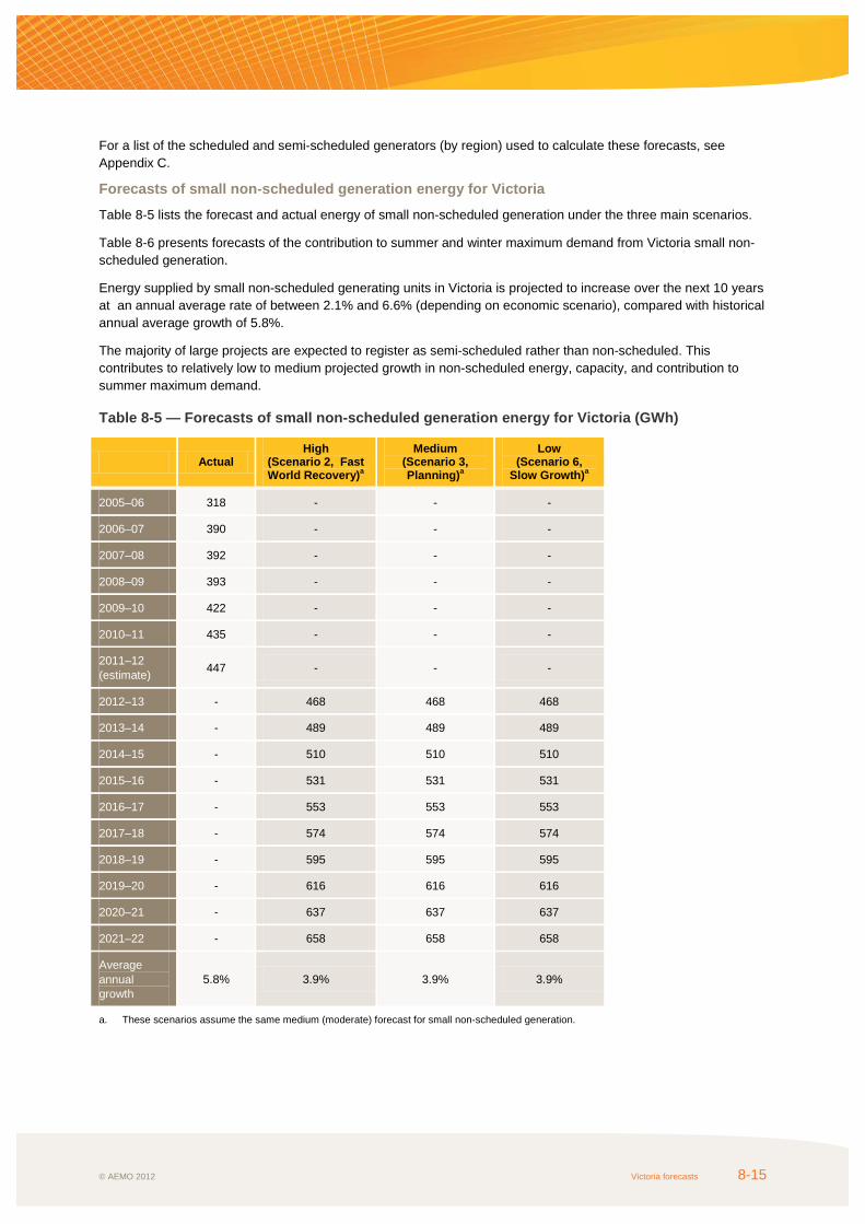
© AEMO 2012 Victoria forecasts 8-15
For a list of the scheduled and semi-scheduled generators (by region) used to calculate these forecasts, see Appendix C.
Forecasts of small non-scheduled generation energy for Victoria
Table 8-5 lists the forecast and actual energy of small non-scheduled generation under the three main scenarios.
Table 8-6 presents forecasts of the contribution to summer and winter maximum demand from Victoria small non-scheduled generation.
Energy supplied by small non-scheduled generating units in Victoria is projected to increase over the next 10 years at an annual average rate of between 2.1% and 6.6% (depending on economic scenario), compared with historical annual average growth of 5.8%.
The majority of large projects are expected to register as semi-scheduled rather than non-scheduled. This contributes to relatively low to medium projected growth in non-scheduled energy, capacity, and contribution to summer maximum demand.
Table 8-5 — Forecasts of small non-scheduled generation energy for Victoria (GWh)
Actual High
(Scenario 2, Fast World Recovery)a
Medium (Scenario 3, Planning)a
Low (Scenario 6,
Slow Growth)a
2005–06 318 - - -
2006–07 390 - - -
2007–08 392 - - -
2008–09 393 - - -
2009–10 422 - - -
2010–11 435 - - -
2011–12 (estimate) 447 - - -
2012–13 - 468 468 468
2013–14 - 489 489 489
2014–15 - 510 510 510
2015–16 - 531 531 531
2016–17 - 553 553 553
2017–18 - 574 574 574
2018–19 - 595 595 595
2019–20 - 616 616 616
2020–21 - 637 637 637
2021–22 - 658 658 658
Average annual growth
5.8% 3.9% 3.9% 3.9%
a. These scenarios assume the same medium (moderate) forecast for small non-scheduled generation.

NATIONAL ELECTRICITY FORECASTING REPORT
8-16 Victoria forecasts © AEMO 2012
Table 8-6 — Forecasts of the small non-scheduled generation contribution to maximum demand for Victoria (MW)
Actual
Summer maximum demand
Actual
Winter maximum demand
High (Scenario 2, Fast World Recovery) a
Medium (Scenario
3, Planning)a
Low (Scenario 6, Slow
Growth)a
High (Scenario 2, Fast World
Recovery)b
Medium (Scenario
3, Planning)b
Low (Scenario 6, Slow
Growth)b
2005–06 37 - - - - - - -
2006–07 36 - - - 23 - - -
2007–08 21 - - - 42 - - -
2008–09 20 - - - 26 - - -
2009–10 39 - - - 33 - - -
2010–11 64 - - - 58 - - -
2011–12 20 - - - 83 - - -
2012–13 - 21 21 21 - 20 20 20
2013–14 - 23 23 23 - 21 21 21
2014–15 - 24 24 24 - 23 23 23
2015–16 - 25 25 25 - 24 24 24
2016–17 - 26 26 26 - 25 25 25
2017–18 - 27 27 27 - 26 26 26
2018–19 - 28 28 28 - 27 27 27
2019–20 - 29 29 29 - 28 28 28
2020–21 - 30 30 30 - 29 29 29
2021–22 - 31 31 31 - 30 30 30
Average annual growth
- 4.0% 4.0% 4.0% - 4.2% 4.2% 4.2%
a. These scenarios assume the same medium (moderate) forecast for small non-scheduled generation.
b. These scenarios assume the same medium (moderate) forecast for small non-scheduled generation.

© AEMO 2012 Regional model equations for non-large industrial consumption A-1
APPENDIX A - REGIONAL MODEL EQUATIONS FOR
NON-LARGE INDUSTRIAL CONSUMPTION
This appendix provides model equations for non-large industrial consumption for each NEM region.
A.1 New South Wales (including the ACT)
The model equation for non-large industrial consumption, which is based on a Vector Error Correction model has
been constructed on a quarterly basis and is outlined as follows:
∆ ln��� � �0.53e����
�0.28∆ ln������ � 0.05∆ ln������ � 0.08∆ ln������
�0.21∆ ln������ � 0.03∆ ln������ � 0.23∆ ln������
�0.15∆ ln������ � 0.26∆ ln������ � 0.07∆ ln������
�0.004�1 � 0.11�2 � 0.10�3
�0.0003� � 0.0002! ∗ �1 � #!�
Where e� � 2.25 � 0.29 ln�p� � 0.62 ln�i� � y
Or y � 2.25 � 0.29 ln�p� � 0.62 ln�i�
• y = per capita electricity consumption in kWh per quarter per person
• i = state final demand per capita in 2009–10 dollars per quarter
• p = real residential electricity price in 2009–10 c/kWh
• HDD = heating degree days per quarter in Sydney (Observatory Hill)
∑ )*+�0, -. � 18� where -. is average daily temperature on a 6:00 PM to 6:00 PM basis
• CDD = cooling degree days per quarter in Sydney (Observatory Hill)
∑ )*+�0,19 � -.� where -. is average daily temperature on a 6:00 PM to 6:00 PM basis
• AC = Air conditioning ownership variable developed by AEMO
• S1 = seasonal dummy for the March quarter (1 when period is the March quarter, 0 otherwise)
• S2 = seasonal dummy for the June quarter (1 when period is the June quarter, 0 otherwise)
• S3 = seasonal dummy for the September quarter (1 when period is the September quarter, 0 otherwise)
Due to the complex nature of the VEC model, it is best to focus on the error component for the long-run driver
relationships. Putting the long-run relationship simply:
� � 2.25 � 0.29 ln��� � 0.62 ln���
Key observations in the short run include:
• Lags of consumption, price and income allow for short-run effects of these variables.
• Heating degree days (the heating load) and cooling degree days (the cooling load) along with an air
conditioning ownership variable explain the short-run variations in electricity consumption.
• Seasonal (quarterly) dummy variables allow adjustment for the non-temperature related quarterly seasonality
in electricity consumption.

NATIONAL ELECTRICITY FORECASTING REPORT
A-2 Regional model equations for non-large industrial consumption © AEMO 2012
Key observations in the long run include:
• Per capita consumption has a fixed component (2.25 kWh per person) and a price elasticity of -0.29, implying
that the long-run response to a 1% increase in electricity price is a 0.29% decrease in electricity consumption.
• Per capita consumption also has an income elasticity of +0.62, meaning that the long-run response to an
increase in state final demand per capita of 1% is a 0.62% increase in electricity consumption.
A.2 Queensland
The model equation for non-large industrial consumption, which is based on an Auto-Regressive Distributed Lag
(ARDL) model has been constructed on a quarterly basis and is outlined as follows:
ln��� � 5.53
�0.26 ln��� � 0.18 ln������ � 0.03 ln�/����
�0.012�1 � 0.012�2 � 0.021�3
�0.00035! � 0.0080
Where:
• y = per capita electricity consumption in kWh per quarter per person
• i = gross state product per capita in 2009–10 dollars per person per quarter
• p = real total electricity price in 2009–10 c/kWh
• r = real interest rate, defined as (((svr/100)+1)/(1+log(cpi/cpi(-4))))-1 where svr is quarterly standard variable
interest rate1 and cpi is quarterly consumer price index
• CDD = cooling degree days per quarter in Brisbane (Archerfield)
∑ )*+�0,21 � -.� where -. is average daily temperature on a 6:00 PM to 6:00 PM basis
• S1 = seasonal dummy for the March quarter (1 when period is the March quarter, 0 otherwise)
• S2 = seasonal dummy for the June quarter (1 when period is the June quarter, 0 otherwise)
• S3 = seasonal dummy for the September quarter (1 when period is the September quarter, 0 otherwise)
• w = dummy for the Queensland floods in 2010–11 (1 for December 2010 quarter, March 2011 quarter and
June 2011 quarter)
Weather components include cooling degree days (the cooling load), and a dummy variable to adjust for the impact
of 2010–11 Queensland floods. Additionally, there are seasonal (quarterly) dummy variables that allow adjustment
for the non-temperature related quarterly seasonality in electricity consumption.
Key observations include:
• Per capita consumption has a fixed component (5.53 kWh per person).
• A lagged total electricity price with elasticity of -0.18, implying that a 1% increase in total electricity price nine
months ago will result in a 0.18% decrease in electricity consumption today.
• A lagged real interest rate with elasticity of -0.03, implying that a 1% increase in real interest rate three months
ago will result in a 0.03% decrease in electricity consumption today.
• A gross state product per capita with income elasticity of +0.26, implying that an increase in gross state
product per capita of 1% will result in a 0.26% increase in electricity consumption.
1Standard variable banks housing loan rates published by Reserve Bank of Australia, Table F5 Indicator Lending Rates.

© AEMO 2012 Regional model equations for non-large industrial consumption A-3
A.3 South Australia
The model equation for non-large industrial consumption, which is based on a Vector Error Correction model, has
been constructed on a quarterly basis and is outlined as follows:
∆ 12��� � �0.823̂���
�0.12∆ 12������ � .08∆ 12����6�
�0.13∆ 12������ � 0.09∆ 12����6�
�0.13∆ 12������ � 0.03∆ 12����6�
�0.007�1 � 0.04�2 � 0.07�3
�0.0004� � 0.0005!
Where
e� � 7.10 � 0.25 ln�p� � 0.34 ln�i� � y Or
y � 7.10 � 0.25 ln�p� � 0.34 ln�i�
• y = per capita electricity consumption in kWh per quarter per person
• i = state final demand per capita in 2009–10 dollars per person per quarter
• p = real residential electricity price in 2009–10 c/kWh
• HDD = heating degree days per quarter in Adelaide (Kent Town)
∑ Max�0, T; � 17.5� where T; is average daily temperature on a 6:00 PM to 6:00 PM basis
• CDD = cooling degree days per quarter in Adelaide (Kent Town)
∑ Max�0,19.5 � T;� where T; is average daily temperature on a 6:00 PM to 6:00 PM basis
• S1 = seasonal dummy for the March quarter (1 when period is the March quarter, 0 otherwise)
• S2 = seasonal dummy for the June quarter (1 when period is the June quarter, 0 otherwise)
• S3 = seasonal dummy for the September quarter (1 when period is the September quarter, 0 otherwise)
Due to the complex nature of the VEC model, it is best to focus on the error component for the long-run driver relationships. Putting the long-run relationship simply:
y � 7.10 � 0.25 ln�p� � 0.34 ln�i�
Key observations in the short run include:
• Lags of consumption, price and income allow for short-run effects of these variables.
• Heating degree days (the heating load) and cooling degree days (the cooling load) along with an air
conditioning ownership variable explain the short-run variations in electricity consumption.
• Seasonal (quarterly) dummy variables allow adjustment for the non-temperature related quarterly seasonality
in electricity consumption.
Key observations in the long run include:
• Per capita consumption has a fixed component (7.10 kWh per person) and a price elasticity of -0.25, implying
that the long-run response to a 1% increase in electricity price is a 0.25% decrease in electricity consumption.
• Per capita consumption also has an income elasticity of +0.34, meaning that the long-run response to an
increase in state final demand per capita of 1% is a 0.34% increase in electricity consumption.

NATIONAL ELECTRICITY FORECASTING REPORT
A-4 Regional model equations for non-large industrial consumption © AEMO 2012
A.4 Tasmania
The model equation for non-large industrial consumption, which is based on a Vector Error Correction model has
been constructed on a quarterly basis and is outlined as follows:
∆ 12��� � �0.583̂���
�0.17∆ 12������ � 0.24∆ 12������ � 0.21∆ 12������ � 0.13∆ 12�<= >?����
�0.05�1 � 0.16�2 � 0.16�3
�0.0004�
Where
3̂ � 2.85 � 0.68 ln��� � 0.69 ln��� � 0.13 ln�<= >?� � � Or
� � 2.85 � 0.68 ln��� � 0.69 ln��� � 0.13 ln�<= >?�
• y = per capita electricity consumption in kWh per quarter per person
• i = state final demand per capita in 2009–10 dollars per person per quarter
• p = real residential electricity price in 2009–10 c/kWh
• INDEX = Gas and Other Household Fuels Price Index (ABS CPI Series 6401)
• HDD = heating degree days per quarter in Hobart (Ellerslie Road)
∑ )*+�0, -. � 19� where -. is average daily temperature on a 6:00 PM to 6:00 PM basis
• S1 = seasonal dummy for the March quarter (1 when period is the March quarter, 0 otherwise)
• S2 = seasonal dummy for the June quarter (1 when period is the June quarter, 0 otherwise)
• S3 = seasonal dummy for the September quarter (1 when period is the September quarter, 0 otherwise)
Due to the complex nature of the VEC model, it is best to focus on the error component for the long-run driver
relationships. Putting the long-run relationship simply:
� � 2.85 � 0.68 ln��� � 0.69 ln��� � 0.13 ln�<= >?�
Key observations in the short run include:
• Lags of consumption, price, income, and the alternative fuels index allow for short-run effects of these
variables.
• Heating degree days (the heating load) explain the short-run variations in electricity consumption.
• Seasonal (quarterly) dummy variables allow adjustment for the non-temperature related quarterly seasonality
in electricity consumption.
Key observations in the long run include:
• Per capita consumption has a fixed component (2.85 kWh per person) and a price elasticity of -0.69, implying
that the long-run response to a 1% increase in electricity price is a 0.69% decrease in electricity consumption.
• Per capita consumption has an income elasticity of +0.69, meaning that the long-run response to an increase
in state final demand per capita of 1%, is a 0.69% increase in electricity consumption.
• The alternative fuel index has an elasticity of 0.13%, meaning that the long-run response to an increase in
alternative fuels of 1% is a 0.13% increase in electricity consumption. The inclusion of this variable was based
on the alternative fuel availability in Tasmania (for example, gas and wood) for heating. However, electricity
price and income are the major determinants of electricity consumption in the mass market sector.

© AEMO 2012 Regional model equations for non-large industrial consumption A-5
A.5 Victoria
The model equation for non-large industrial consumption, which is based on an Auto-Regressive Distributed Lag
(ARDL) model has been constructed on a quarterly basis and is outlined as follows:
ln�y� � 4.54
�0.34 ln�i� � 0.04ln�p� � 0.05 ln�p��6� � 0.046 ln�p���� � 0.096 ln�p����
�0.0026S1 � 0.023S2 � 0.03S3
�0.00032CDD � 0.00037HDD
Where:
• y = per capita electricity consumption in kWh per quarter per person
• i = gross state product per capita in 2009–10 dollars per person per quarter
• p = real residential electricity price in 2009–10 c/kWh
• CDD = cooling degree days per quarter in Melbourne (Melbourne Airport)
∑ Max�0,18 � T;� where T; is average daily temperature on a 6:00 PM to 6:00 PM basis
• HDD = heating degree days per quarter in Melbourne (Melbourne Airport)
∑ Max�0, T � 17.........� where T; is average daily temperature on a 6:00 PM to 6:00 PM basis
• S1 = seasonal dummy for the March quarter (1 when period is the March quarter, 0 otherwise)
• S2 = seasonal dummy for the June quarter (1 when period is the June quarter, 0 otherwise)
• S3 = seasonal dummy for the September quarter (1 when period is the September quarter, 0 otherwise)
The weather components include cooling degree days (the cooling load) and heating degree days (the heating
load). Additionally, there are seasonal (quarterly) dummy variables that allow adjustment for the non-temperature
related quarterly seasonality in electricity consumption.
Key observations include:
• Per capita consumption has a fixed component (4.54 kWh per person).
• A real residential electricity price with elasticity of -0.14, implying that a 1% increase in residential electricity
price during the last 12 months will result in a 0.14% decrease in electricity consumption today.
• A GSP per capita with income elasticity of +0.34, implying that an increase in GSP per capita of 1% will result
in a 0.34% increase in electricity consumption.

NATIONAL ELECTRICITY FORECASTING REPORT
A-6 Regional model equations for non-large industrial consumption © AEMO 2012
[This page is left blank intentionally]

© AEMO 2012 Energy efficiency B-1
APPENDIX B - ENERGY EFFICIENCY
B.1 Introduction B.1.1 Energy efficiency impacts as a post-model adjustment This appendix analyses and forecasts the impact of a range of energy efficiency and greenhouse gas abatement measures on future electricity consumption and maximum demand in the National Electricity Market (NEM). The forecasts are then used together with forecasts of rooftop photovoltaics (PV) as post-model adjustments to the electricity forecasts for non-large industrial consumption produced by econometric modeling in the national electricity forecasting project.
Various policies are in place on both the national and the state level to achieve energy efficiency objectives and to reduce greenhouse gas emissions.
The main national policies reviewed in this forecast are the Clean Energy Future package, the national Renewable Energy Target (RET) scheme, Mandatory Disclosure (Energy Efficiency Disclosure Act 2010), Minimum Energy Performance Standards (MEPS), and various building energy efficiency codes.
Some of the state government energy efficiency policies are measured individually to develop energy efficiency impact forecasts for each state, such as the New South Wales Energy Savings Scheme, South Australian Residential Energy Efficiency Scheme (REES), Queensland Renewable Energy Plan, and the Victorian Energy Efficiency Target (VEET). See Table B-1 for the full list of policy measures covered in this appendix.
The impacts from the assessed policy measures are forecast in both annual energy (gigawatt hours (GWh)) and maximum demand (megawatts (MW)) by region. Maximum demand is expected to be an approximation, as it is less predictable in terms of how households, businesses will behave and appliances will perform during maximum demand events.
The appendix mainly focuses on existing energy efficiency policies or measures affecting the residential sector. The commercial and industrial sector is considered only when the relevant reduction targets are explicitly stated in these policies.
B.1.2 Energy efficiency definition The World Energy Council has defined energy efficiency improvement1 as being a reduction in the energy used for a given service (for example, heating, cooling, and lighting) or level of activity. The reduction in the energy consumption is usually associated with technological changes, but not always, since it can also result from better organization and management or improved economic conditions in the sector (referred to as non-technical factors).
Energy efficiency can result from several areas:
• Individual behaviour to avoid unnecessary consumption of energy, such as switching off lights or air-conditioning when not needed, and the employment of standby power controllers.
• Choosing the most appropriate equipment to reduce energy consumption (such as electrical appliances with higher energy ratings) and better building standards (including installing insulation).
B.1.3 Impacts on demand forecasting Energy efficiency and emission reduction policies, coupled with rising energy prices in recent years, have encouraged households and businesses to undertake energy efficiency measures to reduce their electricity bills.
1 World Energy Council. ‘Energy Efficiency Policies around the World: Review and Evaluation’. Available:
http://www.worldenergy.org/publications/energy_efficiency_policies_around_the_world_review_and_evaluation/1_introduction/1175.asp. Viewed 14 June 2012.

NATIONAL ELECTRICITY FORECASTING REPORT
B-2 Energy efficiency © AEMO 2012
Energy efficiency though policy incentives, technological improvements or consumer behaviour change is expected to have a long-lasting effect on energy and maximum demand in the NEM.
When estimating historical annual energy or forecasting future demand, it is important to account for the contribution from energy efficiency. Omitting the contribution from energy efficiency can result in demand forecast overestimation.
This paper forecasts the impact of energy efficiency policies on electricity demand for the 20-year outlook period from 2012 to 2031. The forecasts are largely based on the existing energy efficiency policies and do not take potential future policy changes into consideration.
The analysis presented here will form part of the electricity forecasts, which will reduce the mass market demand forecasts from the econometric modelling.
In Scenario 2, Fast World Recovery; Scenario 3, Planning; Scenario 4, Decentralised World; Scenario 5, Slow Rate of Change; and Scenario 6, Slow Growth, 50% of the energy efficiency impact is incorporated in the annual energy forecasts and the maximum demand forecasts for each region.
Only Scenario 1, Fast Rate of Change, has assumed a 100% energy efficiency impact.
B.1.4 Future work This is the first time AEMO has undertaken a study of energy efficiency policies that influence electricity demand, which aims to establish a framework for future work and improvement in the following areas:
• Increased collaboration with government agencies, energy efficiency bodies, transmission network service providers (TNSP) and distribution network service providers (DNSP) to understand consumer behaviour changes.
• More closely monitoring the implementation of energy policies and measure the impact of these policies.
• Develop a robust data collection process by appliance and by sector.
• Build accurate inventory for major electrical appliances in the NEM.
• More in-depth analysis and modelling in the following areas:
− Energy efficiency potential in the residential sector.
− Commercial and industrial energy efficiency opportunities.
− Energy efficiency impacts on maximum demand.
• Measuring how electricity prices influence consumer choices and interact with energy efficiency policies.
B.2 Energy efficiency policies, drivers and methodology B.2.1 Energy efficiency policies This section describes current state government and Australian Government policies that might impact electricity demand.
Table B-1 provides an overview of six national policies, some of which are described in more detail in Section B.13.

© AEMO 2012 Energy efficiency B-3
Table B-1 — Key national policies that may impact NEM electricity demand
Table B-2 provides an overview of key state energy efficiency policies that impact electricity demand, which are described in more detail in Section B.14.
2 Clean Energy Future, available at http://www.cleanenergyfuture.gov.au/clean-energy-future/our-plan/. Viewed 25 June 2012. 3 Energy Efficiency Opportunities, available at http://www.ret.gov.au/energy/efficiency/eeo/Pages/default.aspx. Viewed 25 June 2012. 4 Minimum Energy Performance Standards, available at http://www.energyrating.gov.au/. Viewed 25 June 2012. 5 National Framework for Energy Efficiency, available at http://www.ret.gov.au/documents/mce/energy-eff/nfee/committees/buildings/default.html.
View 25 June 2012. 6 Insulation Rebate, available at http://www.australian-government-insulation-rebates.com/Rebates/federal-government-rebate.html. Viewed 25 June
2012. 7 Renewable Energy Target, available at http://www.climatechange.gov.au/ret. Viewed 25 June 2012.
Program Measure Description of impact on electricity demand
Clean Energy Future plan 2 Carbon price, energy efficiency, renewable energy. Impact on generation merit order, price elasticity of demand by sector, and energy efficiency measures.
Energy Efficiency Opportunities Programs 3
Assessment of energy efficiency opportunities from large energy users.
Energy savings, potential renewable energy, cogeneration and trigeneration opportunities.
Minimum Energy Performance Standards (MEPS) 4
Mandatory for a range of electrical products manufactured in or imported into Australia.
Electricity appliance penetration and appliance efficiency.
The Energy Rating Labelling Scheme is a mandatory scheme for a range of appliances, which currently include refrigerators, freezers, clothes washers, clothes dryers, dishwashers, air conditioners and televisions.
Mandatory Disclosure (Energy Efficiency Disclosure Act 2010)5
Residential and commercial energy performance when sold or leased (existing buildings).
Impacts electricity use for space heating/cooling, and lighting.
Home Insulation Program 2009–10 6 Insulation subsidy for existing uninsulated dwellings. Program ended in 2010, but has an
ongoing impact on electricity demand.
Renewable Energy Target (RET) 7
Targeted renewable energy production through a certificate scheme. Hot water eligible.
Impact via switch to solar water heaters and heat pumps.

NATIONAL ELECTRICITY FORECASTING REPORT
B-4 Energy efficiency © AEMO 2012
Table B-2 — Key state policies that may impact NEM electricity demand
B.3 Drivers of energy efficiency Energy efficiency and emission reduction policies, coupled with recent increasing energy prices, have encouraged households and businesses to undertake energy efficiency measures to reduce costs.
A range of activities are accounted for in developing the energy efficiency policy impact forecasts:
• The replacement of incandescent lighting with fluorescent and LED lights.
• The replacement of electric heaters or coolers with gas heaters, heat pumps, or reverse-cycle air-conditioners.
• The replacement of electric hot water systems with gas or solar water heaters.
• The installation standby power controllers and In-home displays.
• The replacement of electrical appliances with appliances with higher energy ratings.
• More energy-efficient building standards.
8 Available at https://www.veet.vic.gov.au/Public/Public.aspx?id=Home. Viewed 25 June 2012. 9 Overview of the Scheme, available at http://www.ess.nsw.gov.au/Overview_of_the_scheme. Viewed 25 June 2012. 10 Queensland Renewable Energy Plan, available at http://www.cleanenergy.qld.gov.au/renewable-energy/renewable-energy-plan.htm. Viewed 25
June 2012. 11 Residential Energy Efficiency Scheme, available at http://www.escosa.sa.gov.au/consumer-information/residential-energy-efficiency-
scheme.aspx. Viewed 25 June 2012. 12 Energy Saving Guide, available at http://www.education.tas.gov.au/dept/strategies/energy-saving-guide. Viewed 25 June 2012.
Jurisdiction Program Measure Description of impact on electricity demand
Victoria Victorian Energy Efficiency Target (VEET)8, Phase Two.
Retailers are required to meet targets mainly through energy efficiency measures.
Impact on electricity demand through lightings upgrade, standby power etc. by residential customers.
New South Wales Energy Savings Scheme9.
Businesses are required to meet targets mainly through energy efficiency measures.
Impact through the surrender of Energy Savings Certificates (ESCs) by residential, commercial and industrial customers undertaking energy saving activities.
Queensland Queensland Renewable Energy Plan10.
Total 2,635 MW renewable energy capacity by 2020, involving Solar Hot Water Rebate, the Solar Bonus Scheme, and The Solar City.
Energy savings on grid through renewable energy incentives.
South Australia South Australian Residential Energy Efficiency Scheme (REES)11.
Energy providers are required to achieve greenhouse gas reduction targets mainly through energy saving measures.
Impact on electricity demand through lighting, showerheads, insulation, heating/cooling, and electric appliances.
Tasmania Energy Saving Guide12.
Educational material for government agencies to address climate change and greenhouse gas emissions.
No real target on energy savings or energy efficiency.

© AEMO 2012 Energy efficiency B-5
B.4 Energy efficiency impact forecast category A range of energy efficient appliances and equipment have been considered:
• Lighting (the phase-out of incandescent light bulbs).
• Heating and cooling systems.
• Hot water systems (the phase-out of electric storage hot water systems).
• Standby power controllers.
• Building standards.
• Other appliances covered by the MEPS.
B.5 Energy efficiency impact base scenario and data sources
Energy efficiency policy impacts are forecast for the medium, base case scenario only, which is used to develop the annual energy and maximum demand forecasts for all scenarios.
The energy efficiency policy impact forecast development is largely based on a series of secondary information sources:
• Government reviews of the energy efficiency programs.
• Consultancy reports.
• Australian Bureaux of Statistics (ABS) demographic and electrical appliance statistics.
• Economic forecasts developed by the National Institute of Economic and Industry Research (NIEIR).
The accuracy of the forecasts depends on the accuracy of this information.
B.6 Estimating energy efficiency policy impacts Three main steps were used to develop the forecasts:
• Step 1, calibrating historical energy efficiency impacts based on ABS household appliances data and electricity demand by NEM region from 2007–08 till 2010–11.
• Step 2, estimating total energy savings using average household consumption patterns from step 1 categorised by lighting, hot water, heating and cooling, standby power, and MEPS, taking into consideration the potential impact of energy efficiency policies.
• Step 3, forecasting the maximum demand based on the annual energy forecasts, and efficiency gains from each category specified in step 2.
Each forecast category is analysed separately for annual energy and maximum demand forecasts based on its distinctive feature in terms of influencing annual energy and maximum demand.
For example, appliances such as commercial lighting and refrigeration, and energy efficient buildings, are more likely to reduce both electricity consumption and maximum demand, whereas other appliances such as televisions, cooking appliances, heating and cooling systems, and hot water systems may have more effect on electricity consumption than maximum demand.

NATIONAL ELECTRICITY FORECASTING REPORT
B-6 Energy efficiency © AEMO 2012
Figure B-1 illustrates the modelling framework for the policy impact forecast.
Figure B-1 — Modelling framework for the policy impact forecast
Where possible, a residential electrical appliance analysis of the following appliances is performed to match historical residential electricity consumption:
• Electric hot water and electric-boosted solar water heaters.
• Electric heating.
• Electric cooling (air-conditioning, refrigerated and evaporative systems).
• Pools and spas (Queensland only).
• Fridges/freezers.
• Washing machines and dryers.
• Electric cooktops and electric ovens.
• Televisions, home theaters and stereos.
• Computers and game consoles.
• Standby power.
Commercial and industrial analysis is performed based on the MEPS only.
ABS Statistics on household appliances
Historical residential electricity consumption
Economic outlook - Household growth
- - AC sales forecasts
Government/consultant research reports
Household electrical appliance analysis Policy analysis
(including commercial/industrial MEPS analysis)
Energy Efficiency Impact
FORECAST
Commercial Energy Efficiency
analysis
IndustrialEnergy Efficiency
analysis

© AEMO 2012 Energy efficiency B-7
B.7 Modelling limitations The energy efficiency policy impact forecasts are primarily based on existing policies and measures with real energy savings targets, and potential policy changes are not considered or assessed.
Policies on the national level and policies on the state level may not be mutually exclusive. For example, in the water heating area, a number of measures currently exist in parallel on a both national and a state level, including rebates for replacing electric resistance water heating, state solar water heater rebates, building standards, and eligibility of solar water heating for the national RET scheme.
The forecast categories in some cases may overlap with each other. Energy efficient lighting, heating and cooling systems, hot water systems are potentially also covered in the Building Standards. To minimise the possibility of double counting, a growth rate for each appliance is assumed.
The impact on electricity consumption co-exists in both electricity price response, energy efficiency and the uptake of distributed energy such as rooftop PV. The interaction among these three aspects is not analysed in this report and the potential overlap is not measured in these forecasts.
In addition, rebound effects, for example using more efficient lighting, the rebound effect may off-set the potential energy saving. Lighting, space conditioning (air conditioning and heating) and hot water use are likely to have an element of rebound.
The rebound effects are not analysed and therefore not measured in these forecasts.
B.8 Energy efficiency policy impacts in the NEM AEMO independently studied energy efficiency policy impacts to understand the current and forecast impact of energy efficiency policies on the NEM. This is the first time AEMO has undertaken a study of this type, and the methodology will continue to develop. This first step has, however, provided insight into the current setting of energy efficiency policies and their impacts on the NEM.
Various energy efficiency program reviews and consultancy reports are available, mostly targeting individual programs, some of which have been incorporated into the forecasts.
The historical and forecast estimates for the NEM are an aggregation of each of the five regions.
The analysis discussed here forms the basis for AEMO’s energy forecast calculations.
B.9 Historical analysis The impact of energy efficiency on overall electricity demand in the NEM has become noticeable over the last few years. This has been reflected in the average consumption per household, estimated using ABS household appliances data and electricity demand by NEM region from 2007–08 to 2010–11.
Estimates suggest that the regions with mandatory residential energy efficiency targets have seen a reduction of average household electricity consumption over this period.
This reduction was largely a result of more efficient lighting and electrical appliances, better energy ratings in building standards, and a certain degree of behaviour changes responding to the increased energy prices.
Table B-3 lists the estimated average daily consumption per household in kWh in 2004–05, 2007–08 and 2010–11.

NATIONAL ELECTRICITY FORECASTING REPORT
B-8 Energy efficiency © AEMO 2012
Table B-3 — Estimated average daily consumption per household in kWh by NEM region in 2004–05, 2007–08 and 2010–11
Daily consumption per household (kwh) 2004–05 2007–08 2010–11
Victoria 16.37 17.68 16.07
Queensland 21.38 21.57 22.14
New South Wales (and the ACT) 17.94 18.00 17.74
South Australia 17.65 18.15 17.82
Tasmania 27.80 27.47 29.56
Figure B-2 shows the breakdown of estimated residential electricity consumption by appliance in the NEM.
Figure B-2 — Residential electricity consumption by appliance in the NEM
B.10 Annual energy Figure B-3 shows the forecast energy saving for energy efficiency for each NEM region in 2011–12, 2021–22 and 2031–32.
In the NEM, annual energy savings due to energy efficiency policy impacts are forecast to reach approximately 14,191 GWh by 2021–22 and 21,032 GWh by 2031–32.
Lighting, 10%
Hot Water, 18%
Heating/Cooling, 20%
Fridges/Freezers, 11%
Washers/Dryers, 7%
Dishwashers, 3%
Cooktops/Stove, 6%
TV, 3%
Electronics, 4%
Standby, 4%Pool, 4%
Others, 10%
Lighting Hot Water Heating/Cooling Fridges/Freezers Washers/Dryers Dishwashers
Cooktops/Stove TV Electronics Standby Pool Others
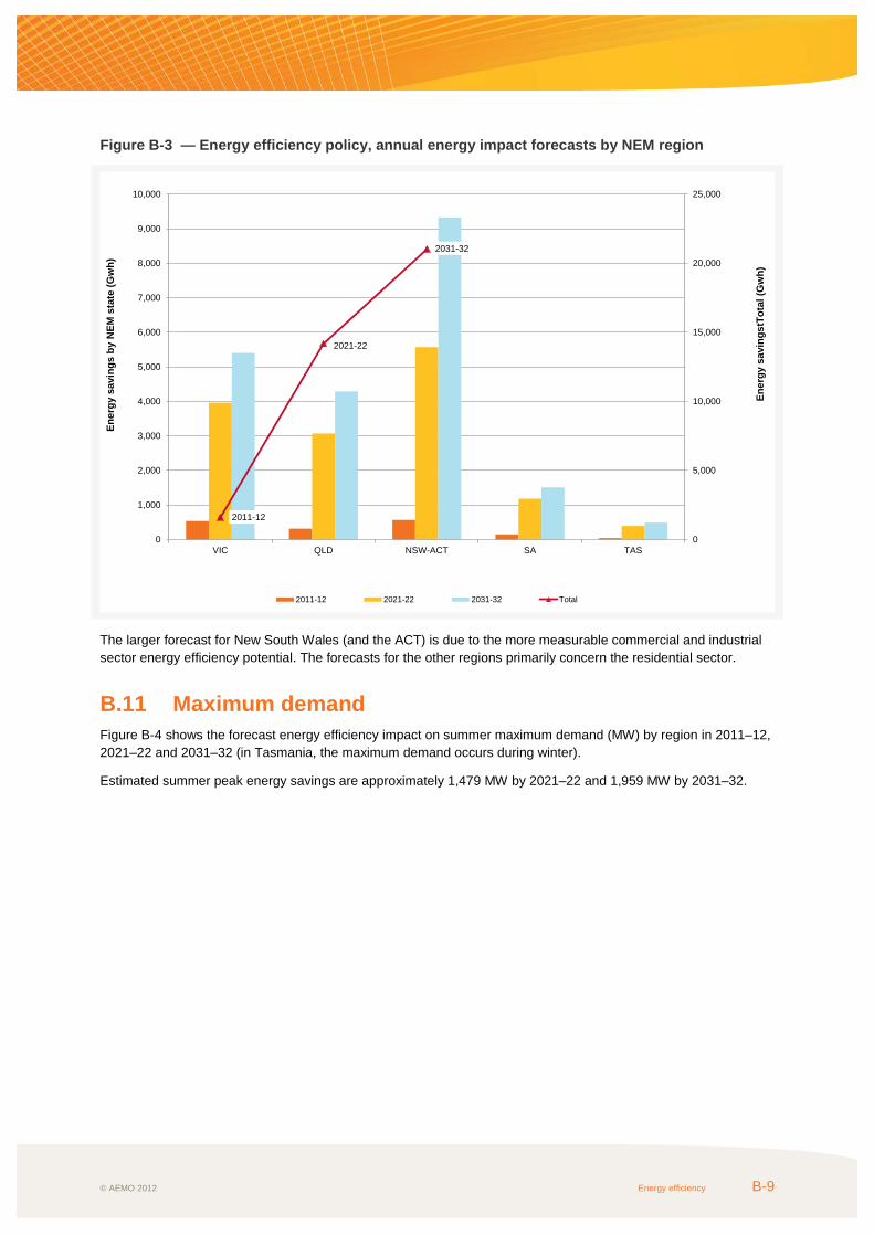
© AEMO 2012 Energy efficiency B-9
Figure B-3 — Energy efficiency policy, annual energy impact forecasts by NEM region
The larger forecast for New South Wales (and the ACT) is due to the more measurable commercial and industrial sector energy efficiency potential. The forecasts for the other regions primarily concern the residential sector.
B.11 Maximum demand Figure B-4 shows the forecast energy efficiency impact on summer maximum demand (MW) by region in 2011–12, 2021–22 and 2031–32 (in Tasmania, the maximum demand occurs during winter).
Estimated summer peak energy savings are approximately 1,479 MW by 2021–22 and 1,959 MW by 2031–32.
2011-12
2021-22
2031-32
0
5,000
10,000
15,000
20,000
25,000
0
1,000
2,000
3,000
4,000
5,000
6,000
7,000
8,000
9,000
10,000
VIC QLD NSW-ACT SA TAS
Ener
gy s
avin
gstT
otal
(Gw
h)
Ener
gy s
avin
gs b
y N
EM s
tate
(Gw
h)
2011-12 2021-22 2031-32 Total

NATIONAL ELECTRICITY FORECASTING REPORT
B-10 Energy efficiency © AEMO 2012
Figure B-4 — Energy efficiency policy, summer maximum demand impact forecasts by NEM region
B.12 Regional energy efficiency policy impact This section provides information about historical and forecast estimates for energy efficiency policy impact in each region. Providing an initial overall picture of energy efficiency policy impacts, additional modelling and data mining work is required to improve the forecasts.
B.12.1 New South Wales (and the Australian Capital Territory) The New South Wales Energy Savings Scheme13 is the key policy considered in developing forecasts for energy efficiency for New South Wales (including the Australian Capital Territory). For an overview of the scheme and the assumptions made in developing these forecasts, see Section B.14.1.
Annual energy
Figure B-5 shows the forecast impact from energy efficiency for New South Wales (including the Australian Capital Territory).
The impact is forecast to grow continuously during the forecast period in both the residential and business sectors (with residential sector growth anticipated to slow after 2021 due to high saturation), and is estimated to reach 5,575 GWh by 2021–22 and 9,331 GWh by 2031–32, which is approximately 7.2% and 11.5% (respectively) of total forecast sent-out energy in New South Wales (including the ACT).
13 See note 9.
2011-12
2021-22
2031-32
0
500
1,000
1,500
2,000
2,500
0
100
200
300
400
500
600
700
VIC QLD NSWACT SA TAS
Sum
mer
max
imum
dem
and
Tota
l (M
W)
Sum
mer
max
imum
dem
and
by N
EM s
tate
(MW
)
2011-12 2021-22 2031-32 Total

© AEMO 2012 Energy efficiency B-11
Figure B-5 — Energy efficiency impact annual energy forecasts for New South Wales (and the Australian Capital Territory)
Maximum demand
Figure B-6 and Figure B-7 show energy efficiency policy impact summer and winter maximum demand forecasts.
Energy efficiency policy summer maximum demand impacts reach 487 MW in 2021–22 and 630 MW in 2031–32.
The winter maximum demand impact is estimated to be similar to the summer maximum demand, because improved energy efficient lighting, refrigeration, and building is most likely to consistently impact in both summer and winter.
0
1,000
2,000
3,000
4,000
5,000
6,000
Annu
al e
nerg
y (G
wh)
Year
Non-residential Residential

NATIONAL ELECTRICITY FORECASTING REPORT
B-12 Energy efficiency © AEMO 2012
Figure B-6 — Energy efficiency impact summer maximum demand forecasts for New South Wales (and the Australian Capital Territory)
Figure B-7 — Energy efficiency impact winter maximum demand forecasts for New South Wales (and the Australian Capital Territory)
0
100
200
300
400
500
600
Sum
mer
max
imum
dem
and
(MW
)
Year
Non-residential Residential
0
100
200
300
400
500
600
2012 2013 2014 2015 2016 2017 2018 2019 2020 2021
Win
ter m
axim
um d
eman
d (M
W)
Year
Non-residential Residential

© AEMO 2012 Energy efficiency B-13
B.12.2 Queensland The Queensland Renewable Energy Plan14 is the key policy considered in developing forecasts for energy efficiency for Queensland. For an overview of the scheme and the assumptions made in developing these forecasts, see Section B.14.2.
Annual energy
Figure B-8 shows the forecast impact from energy efficiency for Queensland.
The impact is forecast to grow continuously during the forecast period in both the residential and business sectors, and is estimated to reach 3,072 GWh by 2021–22 and 4,291 GWh by 2031–32, which is approximately 4.7% and 6.0% (respectively) of total forecast sent-out energy in Queensland.
Figure B-8 — Energy efficiency impact annual energy forecasts for Queensland
14 See note 10.
0
500
1000
1500
2000
2500
3000
3500
Annu
al e
nerg
y (G
wh)
Year
Non-residential Residential

NATIONAL ELECTRICITY FORECASTING REPORT
B-14 Energy efficiency © AEMO 2012
Maximum demand
Figure B-9 and Figure B-10 show energy efficiency policy impact summer and winter maximum demand forecasts.
Energy efficiency policy summer maximum demand impacts reach 425 MW in 2021–22 and 589 MW in 2031–32.
The winter maximum demand impact is estimated to be slightly lower than the summer maximum demand based on the assumption that the cooling requirement is lower in winter.
Figure B-9 — Energy efficiency impact summer maximum demand forecasts for Queensland
0
50
100
150
200
250
300
350
400
450
Sum
mer
max
imum
dem
and
(MW
)
Year
Non-residential Residential

© AEMO 2012 Energy efficiency B-15
Figure B-10 — Energy efficiency impact winter maximum demand forecasts for Queensland
B.12.3 South Australia The South Australian Residential Energy Efficiency Scheme (REES)15 is the key policy considered in developing forecasts for energy efficiency for South Australia. For an overview of the scheme and the assumptions made in developing these forecasts, see Section B.14.3.
Annual energy
Figure B-11 shows the forecast impact from energy efficiency for South Australia.
The impact is forecast to grow continuously during the forecast period in both the residential and business sectors, and is estimated to reach 1,186 GWh by 2021–22 and 1,512 GWh by 2031–32, around 8.4% and 10.7% (respectively) of total forecast sent-out energy in South Australia.
15 See note 11.
0
50
100
150
200
250
300
350
400
2012 2013 2014 2015 2016 2017 2018 2019 2020 2021
Win
ter m
axim
um d
eman
d (M
W)
Year
Non-residential Residential
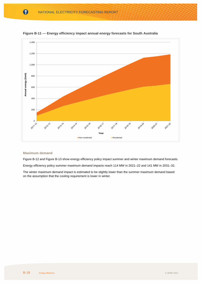
NATIONAL ELECTRICITY FORECASTING REPORT
B-16 Energy efficiency © AEMO 2012
Figure B-11 — Energy efficiency impact annual energy forecasts for South Australia
Maximum demand
Figure B-12 and Figure B-13 show energy efficiency policy impact summer and winter maximum demand forecasts.
Energy efficiency policy summer maximum demand impacts reach 114 MW in 2021–22 and 141 MW in 2031–32.
The winter maximum demand impact is estimated to be slightly lower than the summer maximum demand based on the assumption that the cooling requirement is lower in winter.
0
200
400
600
800
1,000
1,200
1,400
Annu
al e
nerg
y (G
wh)
Year
Non-residential Residential

© AEMO 2012 Energy efficiency B-17
Figure B-12 — Energy efficiency impact summer maximum demand forecasts for South Australia
Figure B-13 — Energy efficiency impact winter maximum demand forecasts for South Australia
0
20
40
60
80
100
120
Sum
mer
max
imum
dem
and
(MW
)
Year
Non-residential Residential
0
20
40
60
80
100
120
2012 2013 2014 2015 2016 2017 2018 2019 2020 2021
Win
ter m
axim
um d
eman
d (M
W)
Year
Non-residential Residential

NATIONAL ELECTRICITY FORECASTING REPORT
B-18 Energy efficiency © AEMO 2012
B.12.4 Tasmania The Energy Saving Guide16 published by the Tasmanian Government has no material measures for energy efficiency. National energy efficiency policies (such as the MEPS) represent the key policies in developing the forecast for Tasmania. For an overview of the MEPS, see Section B.13.5.
Annual energy
Figure B-14 shows the forecast impact from energy efficiency for Tasmania.
The impact is forecast to grow continuously during the forecast period in both the residential and business sectors, and is estimated to reach 396 GWh by 2021–22 and 493 GWh by 2031-32, which is approximately 3.5% and 4.0% (respectively) of total forecast sent-out energy in Tasmania.
Figure B-14 — Energy efficiency impact annual energy forecasts for Tasmania
Maximum demand
Figure B-15 and Figure B-16 show energy efficiency policy impact summer and winter maximum demand forecasts.
Energy efficiency policy summer maximum demand impacts reach 31 MW in 2021–22 and 35 MW in 2031–32.
The winter maximum demand impact is estimated to be slightly higher than summer due to Tasmanian electricity consumption peaking during winter.
16 See note 12.
0
50
100
150
200
250
300
350
400
450
Annu
al e
nerg
y (G
wh)
Year
Non-residential Residential

© AEMO 2012 Energy efficiency B-19
Figure B-15 — Energy efficiency impact summer maximum demand forecasts for Tasmania
Figure B-16 — Energy efficiency impact winter maximum demand forecasts for Tasmania
0
5
10
15
20
25
30
35
Sum
mer
max
imum
dem
and
(MW
)
Year
Non-residential Residential
0
5
10
15
20
25
30
35
40
2012 2013 2014 2015 2016 2017 2018 2019 2020 2021
Win
ter m
axim
um d
eman
d (M
W)
Year
Non-residential Residential

NATIONAL ELECTRICITY FORECASTING REPORT
B-20 Energy efficiency © AEMO 2012
B.12.5 Victoria The Victorian Energy Efficiency Target17 (VEET) scheme is the key policy considered in developing forecasts for energy efficiency for Victoria. For an overview of the scheme and the assumptions made in developing these forecasts, see Section B.14.4.
Annual energy
Figure B-17 shows the forecast impact from energy efficiency for Victoria.
The impact is more significant in the residential sector than in the business sector during the forecast period, due to financial incentives from the VEET scheme. The impact is estimated to reach 3,962 GWh by 2021–22 and 5,404 GWh by 2031–32, which is approximately 7.3% and 9.2% (respectively) of total forecast sent-out energy in Victoria.
Figure B-17 — Energy efficiency impact annual energy forecasts for Victoria
Maximum demand
Figure B-18 and Figure B-19 show energy efficiency policy impact summer and winter maximum demand forecasts.
Energy efficiency policy summer maximum demand impacts reach 421 MW in 2021–22 and 563 MW in 2031–32.
The winter maximum demand impact is estimated to be lower than the summer maximum demand due to a higher percentage of gas heating in Victoria.
17 See note 8.
0
500
1,000
1,500
2,000
2,500
3,000
3,500
4,000
4,500
Annu
al e
nerg
y (G
wh)
YearNon-residential Residential

© AEMO 2012 Energy efficiency B-21
Figure B-18 — Energy efficiency impact summer maximum demand forecasts for Victoria
Figure B-19 — Energy efficiency impact winter maximum demand forecasts for Victoria
0
50
100
150
200
250
300
350
400
450
Sum
mer
max
imum
dem
and
(MW
)
Year
Non-Residential Residential
0
50
100
150
200
250
300
350
400
2012 2013 2014 2015 2016 2017 2018 2019 2020 2021
Win
ter m
axim
um d
eman
d (M
W)
Year
Non-Residential Residential

NATIONAL ELECTRICITY FORECASTING REPORT
B-22 Energy efficiency © AEMO 2012
B.13 National energy efficiency policies B.13.1 Clean Energy Future Plan On 8 November 2011, the Australian Government’s Clean Energy Future Plan18 was passed into law. Under the plan, Australia will reduce greenhouse gas pollution by at least 5% (compared with 2000 levels) by 2020, equivalent to removing 159 Mt/yr CO2-e from the atmosphere by 2020.
The legislation includes the following measures:
• Pricing carbon pollution.
• Promoting innovation and investment in renewable energy.
• Improving energy efficiency.
• Creating opportunities in the land-use sector to cut carbon pollution.
Carbon price
The introduction of a carbon price mechanism was announced by the Australian Government in July 2011, after an agreement reached by the Multi-Party Climate Change Committee.19
Recent modelling work by Treasury for the Australian Government’s Clean Energy Future Plan has led to several carbon price assumptions:
• Fixed carbon pricing will start on 1 July 2012, at a nominal price of $23/t CO2-e, rising to 2.5% in real terms for the subsequent two years.
• A flexible phase will be introduced on 1 July 2015, with the carbon price determined through an emission trading scheme (ETS) with a transitional price cap and floor applied.
• Real growth in the carbon price of 5% per year on average plus inflation from 2015–16 onwards.
This legislation is designed to achieve a reduction in Australian carbon emissions of 5% below 2000 levels by 2020 with a long-term target to cut pollution by 80% below 2000 levels by 2050.
Clean Energy Finance Corporation
A $10 billion commercially oriented Clean Energy Finance Corporation will drive innovation through investments in clean energy. The corporation will leverage private sector financing for renewable energy and clean technology projects, with a focus on renewable energy, energy efficiency, and low-emissions technologies, and the transformation of existing manufacturing businesses to refocus on meeting demand for inputs for these sectors.
National Energy Savings Initiative (ESI)
Under the Clean Energy Future Plan, the Australian Government committed to do further work to investigate the merits of a national Energy Savings Initiative (ESI)20, which will place obligations on energy retailers to find and implement energy savings in households and businesses. The design of any national scheme will need the following features:
• A broad coverage involving the residential, commercial and industrial sectors.
• Creation of an incentive or a requirement to create certificates in both low-income households and in ways that reduce peak demand.
18 See note 2. 19 The Australian Government’s Treasury and the Department of Climate Change and Energy Efficiency modelled the potential economic impacts of
reducing emissions over the medium and long term proposed in the ‘Strong Growth, Low Pollution, Modelling a Carbon Price’ Report, released on 10 July 2011, available http://archive.treasury.gov.au/carbonpricemodelling/content/default.asp. Viewed May 2012.
20 Australian Government, available at http://www.climatechange.gov.au/government/initiatives/energy-savings-initiative.aspx. Viewed 20 June 2012.

© AEMO 2012 Energy efficiency B-23
Subject to the findings of economic modelling and regulatory impact analysis, the Australian Government will make a final decision to adopt a national ESI, which will be conditional on the agreement of the Council of Australian Governments (COAG) and the abolition of existing and planned state schemes.
B.13.2 Renewable Energy Target The national Renewable Energy Target (RET) scheme requires 20% of Australia’s electricity to be produced from renewable energy sources by 2020.21 The scheme requires Australian electricity retailers and large wholesale purchasers of electricity to meet annual targets, creating a financial incentive for investment in renewable energy sources through the creation and sale of certificates. The scheme is split into two parts:
• The Large-scale Renewable Energy Target (LRET) has a target of 41,000 GWh by 2020 and only large-scale renewable energy projects are eligible.
• The Small-scale Renewable Energy Scheme (SRES) targets a theoretical 4,000 GWh annually and is eligible only to small-scale or household installations.
Solar water heaters and heat pumps remain supported through the SRES. Under this scheme, these are assigned a number of Small-scale Technology Certificates (STCs). For information about these policies, see Section 0.
B.13.3 Energy Efficiency Opportunities Regulations The Energy Efficiency Opportunities Act 2006 mandates that corporations that individually or as part of a corporate group use more than 0.5 PJ of energy per year must report on energy savings opportunities with a less than four year payback, and report on their implementation. The first phase of the Energy Efficiency Opportunities (EEO) program extended over the period 2006 to 2011. The second phase covering the period 2012 to 2017 is now being planned.
The program applies to over 310 corporations from the manufacturing, mining, resource processing, electricity generation, transport and commercial sectors. These corporations represent approximately 57% of Australia’s total energy use.
As part of the Australian Government's Clean Energy Future plan, the EEO program will be expanded in the following ways22:
• Extending base funding for the program to 30 June 2017.
• Expanding the program to include energy transmission and distribution networks, and major greenfield and expansion projects, as recommended in the 2010 Prime Minister's Task Group on Energy Efficiency.
• Establishing a voluntary scheme for medium-sized energy users. The Government aims to have the temporary exemption of this sector removed from the EEO regulations by 1 July 2012, and a stakeholder consultation is currently underway. Under the expansion, network businesses that use more than 0.5 PJ of energy in a financial year will be required to register for the EEO program. Energy use is intended to include both own use (such as the fuel used in gas pipeline compressors), and a network's energy losses.
B.13.4 Residential and commercial building mandatory disclosure From 1 November 2010 under the Building Energy Efficiency Disclosure Act 2010, commercial mandatory disclosure requires most sellers or lessors of office space of 2,000 or more square metres to obtain and disclose an up-to-date energy efficiency rating.23 New commercial building standards and promotion of higher star ratings is promoting better energy performance investment in new and existing buildings. This will reduce energy demand for these buildings.
21 See note 7. 22 See note 3. 23 Australian Government, available http://www.cbd.gov.au/LegalResponsibilities.aspx. Viewed 20 June 2012.
NATIONAL ELECTRICITY FORECASTING REPORT
B-24 Energy efficiency © AEMO 2012
The Standing Council on Energy and Resources released the Regulatory Impact Statement for Residential Mandatory Disclosure24 on 21 July 2011, detailing the options under consideration for implementing this legislation, and signalling the start of the public consultation process.
A draft National Building Energy Standard-Setting, Assessment and Rating Framework25 is going through a public consultation process to develop a Framework–Policy Statement for consideration by governments in early 2013.
The Draft Framework is open to feedback on specific policy proposals to provide direction on future energy efficiency standards that involve the following:
• Increasingly stringent minimum building standards set over time for new buildings and renovations.
• Covering all types of residential and commercial buildings, including new and existing buildings.
• Including building equipment and services as well as the building envelope in energy efficiency ratings.
• Improving the accuracy of building performance assessments and ratings through consistent measurement and reporting.
• Encouraging innovation and flexibility to meet defined performance standards.
• Increasing compatibility amongst rating tools used for existing and new buildings.
• Including broader sustainability issues over time, including the level of greenhouse gas emissions generated and water used by buildings.
• Continuing a star ratings approach to communicating building performance.
• Facilitating effective monitoring and compliance.
B.13.5 Minimum Energy Performance Standards Mandatory Minimum Energy Performance Standards (MEPS) and Energy Rating Labels26 are implemented through a collaborative initiative called the Equipment Energy Efficiency Program involving representatives drawn from all jurisdictions in Australia and New Zealand.
It is mandatory for a range of electrical products manufactured in or imported into Australia to meet the MEPS levels specified in the relevant Australian Standards.
The Energy Rating Labelling Scheme is a mandatory scheme for a range of appliances, which currently include refrigerators, freezers, clothes washers, clothes dryers, dishwashers, air conditioners and televisions.
The report “Prevention is Cheaper than Cure – Avoiding Carbon Emissions through Energy Efficiency”27, published by the E3 committee, is used as a guide to measure the energy efficiency impact on residential and non-residential sectors for each NEM region.
B.13.6 Energy Efficiency Building Standards The 2010 Building Code of Australia (BCA), which takes effect from 1 May 2010, will require all new houses to be built in Australia to a six-star energy efficiency rating equivalence28,29. Apartments will have to have an average rating of six stars or equivalent.
24 See note 6. 25 Australian Government, available at http://www.climatechange.gov.au/government/submissions/national-building-framework.aspx. Viewed 20
June 2012. 26 Australian Government, available http://www.energyrating.gov.au/. Viewed 20 June 2012. 27 “Prevention is Cheaper than Cure – Avoiding Carbon Emissions through Energy Efficiency”. An initiative forming part of the Australian National
Framework for Energy Efficiency and the New Zealand National Energy Efficiency and Conservation Strategy, January 2009 28 Building Commission, available http://www.buildingcommission.com.au/www/html/2562-introduction-of-6-star.asp. Viewed 20 June 2012. 29 ACT Government, available http://www.actpla.act.gov.au/customer_information/industry/bca_2010_energy_efficiency_changes. Viewed 20 June
2012.

© AEMO 2012 Energy efficiency B-25
Following the establishment of the BCA, each NEM region has introduced its own energy efficiency building standards. Table B-4 lists the time of the introduction, and summarises the building standard.
Table B-4 — State building standards
Jurisdiction Year of introduction Measure Description of impact on electricity demand
Victoria 1 May 2011. 6-Star Building Standards.
The 6-Star Standard applies to the thermal performance of a new home, home renovations, alterations, additions and relocations plus the requirement to install a solar water heater system or a rainwater tank for toilet flushing in new homes
New South Wales October 2005.
NSW BAXIS program (minimum 5-star energy equivalence rating).
All new dwellings in the state to commit to mandatory water and emission (energy) reduction targets based on the 40% fewer greenhouse gases and 40% less water requirement.
Australian Capital Territory
1 July 2006. Minimum five star energy efficiency rating.a
All new houses must comply with minimum five star energy efficiency rating.
Queensland 1 May 2010 6 Star Building Standards.
New houses and townhouses, and major renovations to existing buildings, must achieve a minimum 6-star energy equivalence rating.b New unit buildings and major renovations to units must achieve a 5-star energy equivalence rating.
South Australia
September 2010.
Mandatory 5 star building standards.
All new homes and extensions built in South Australia need to achieve a 6-star level of energy efficiency.c In addition to achieving a 6-star level for thermal comfort, new houses must also meet lighting requirements and have energy-efficient water heaters.
Tasmania 1 January 2010. 5 star building standards. Energy efficiency requirements apply to the construction or alteration of houses.d
a. “Towards more solar efficient housing Issues Paper”, ACT Planning & Land Authority, July 2008.
b. Available at http://www.dlgp.qld.gov.au/sustainable-housing/6-star-energy-equivalence-rating-requirement-for-houses-and-townhouses.html
c. South Australian Government, availablehttp://sa.gov.au/subject/Housing%2C+property+and+land/Building+and+development/ Residential+building+regulations/Building+rules%2C+regulations+and+information/ Sustainability+and+efficiency+regulations/Six+star+energy+efficiency+requirements+for+new+homes. Viewed 20 June 2012.
d. Tasmanian Government, available http://www.wst.tas.gov.au/industries/building/bca/5_star_energy. Viewed 20 June 2012.
Six Star homes are projected to use 24% less energy through heating and cooling compared to 5 Star homes.30 A 20% energy saving is assumed for all new homes in this forecast.
30 Building Commission, available http://www.buildingcommission.com.au/www/html/2562-introduction-of-6-star.asp. Viewed 20-year outlook period
June 2012.

NATIONAL ELECTRICITY FORECASTING REPORT
B-26 Energy efficiency © AEMO 2012
B.13.7 Phase-out of Electric Storage Hot Water Systems and Solar Hot Water Rebate Phase-out of Electric Hot Water Systems
The Australian Government as part of its National Strategy for Energy Efficiency31 has announced a phase out of greenhouse intensive electric hot water systems from new buildings from 2011.
The restrictions have been placed on the installation of greenhouse intensive water heaters in new detached, terrace, row and town houses (Class 1 buildings under the Building Code of Australia 2010). These regulations apply in all jurisdictions except Tasmania.
Solar Hot Water Rebate
On 28 February 2012, the Australian Government announced the end of the Renewable Energy Bonus Scheme (REBS) by 30 June 2012.32 The Federal Solar Hot Water Rebate will be concluded as a part of the REBS.
Solar water heater systems remain supported through the SRES. Under this scheme, solar and heat-pump water heater systems are assigned a number of Small-scale Technology Certificates (STCs).
Some state rebates on solar water heater systems still exist. A list of Australian, state and territory government solar water heater initiatives up to April 2012 can be found on Clean Energy Council’s website.33
These initiatives have provided incentives to install more energy-efficient solar water heater systems to replace electric hot water systems.
Yearly replacement rates of electric hot water systems are applied to estimate the energy efficiency impact on annual energy consumption. Its impact on maximum demand is assumed to be zero.
B.14 State energy efficiency policies B.14.1 New South Wales Energy Savings Scheme The New South Wales Energy Savings Scheme (ESS)34 establishes legislated annual energy savings targets that must be met through the creation and surrender of energy saving certificates (ESC). In the first year, the target has been set to 0.4% of total electricity sales, increasing to 4% over the period to 2014.
The energy savings target is allocated each year to electricity retailers in proportion to their liable electricity sales, which are total sales less sales to partially exempt, emissions-intensive trade-exposed industries or activities. The list of activities that are partially exempt under the ESS takes into account the national approach to exemptions for the expanded RET scheme and the proposed Carbon Pollution Reduction Scheme (CPRS). If exemptions were not included, the mandated energy savings requirement for retailers would start at 0.5% of liable sales, then increase to 5% by 2014 and continue at that level until 2020. Table B-5 — lists the target’s gradual increase until 2014, after which it remains constant until 2020.
31 Phase-out of greenhouse intensive hot water heaters, available at http://www.climatechange.gov.au/en/what-you-need-to-know/appliances-and-
equipment/hot-water-systems.aspx. Viewed 25 June 2012.. 32 Renewable Energy Bonus Scheme - Solar hot water rebate, Department of Climate Change and Energy Efficiency. 33 Government Initiatives, available at http://www.cleanenergycouncil.org.au/resourcecentre/Government-Initiatives.html. Viewed 25 June 2012. 34 See note 9.
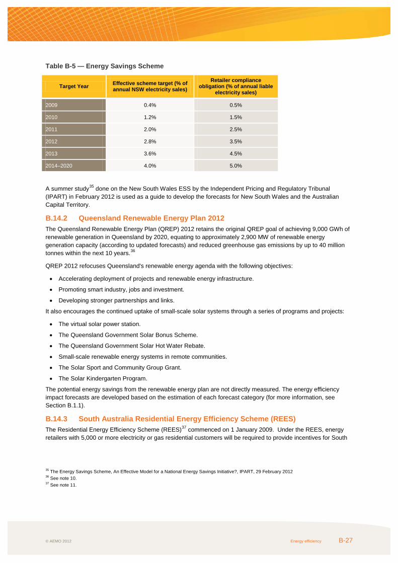
© AEMO 2012 Energy efficiency B-27
Table B-5 — Energy Savings Scheme
Target Year Effective scheme target (% of annual NSW electricity sales)
Retailer compliance obligation (% of annual liable
electricity sales)
2009 0.4% 0.5%
2010 1.2% 1.5%
2011 2.0% 2.5%
2012 2.8% 3.5%
2013 3.6% 4.5%
2014–2020 4.0% 5.0%
A summer study35 done on the New South Wales ESS by the Independent Pricing and Regulatory Tribunal (IPART) in February 2012 is used as a guide to develop the forecasts for New South Wales and the Australian Capital Territory.
B.14.2 Queensland Renewable Energy Plan 2012 The Queensland Renewable Energy Plan (QREP) 2012 retains the original QREP goal of achieving 9,000 GWh of renewable generation in Queensland by 2020, equating to approximately 2,900 MW of renewable energy generation capacity (according to updated forecasts) and reduced greenhouse gas emissions by up to 40 million tonnes within the next 10 years.36
QREP 2012 refocuses Queensland's renewable energy agenda with the following objectives:
• Accelerating deployment of projects and renewable energy infrastructure.
• Promoting smart industry, jobs and investment.
• Developing stronger partnerships and links.
It also encourages the continued uptake of small-scale solar systems through a series of programs and projects:
• The virtual solar power station.
• The Queensland Government Solar Bonus Scheme.
• The Queensland Government Solar Hot Water Rebate.
• Small-scale renewable energy systems in remote communities.
• The Solar Sport and Community Group Grant.
• The Solar Kindergarten Program.
The potential energy savings from the renewable energy plan are not directly measured. The energy efficiency impact forecasts are developed based on the estimation of each forecast category (for more information, see Section B.1.1).
B.14.3 South Australia Residential Energy Efficiency Scheme (REES) The Residential Energy Efficiency Scheme (REES)37 commenced on 1 January 2009. Under the REES, energy retailers with 5,000 or more electricity or gas residential customers will be required to provide incentives for South
35 The Energy Savings Scheme, An Effective Model for a National Energy Savings Initiative?, IPART, 29 February 2012 36 See note 10. 37 See note 11.

NATIONAL ELECTRICITY FORECASTING REPORT
B-28 Energy efficiency © AEMO 2012
Australian households to achieve greenhouse gas reductions and potentially lower their energy bills through reduced energy consumption.
The first stage of the scheme was in operation from 2009–2011. The second stage runs from 2012–2014.
Table B-6 lists the annual greenhouse gas reduction targets (expressed in tonnes of carbon dioxide equivalent) for the first and second REES stages.
Table B-6 — Annual greenhouse gas reduction targets for REES stage 1 and 2 (CO2-e tonnes)
Energy efficiency activities targets
2009 2010 2011 2012 2013 2014
Total 155,000 235,000 255,000 255,000 335,000 410,000
Electricity 136,446 208,423 226,206 226,206(e) 297,173(e) 363,704(e)
(e). Estimated annual targets from electricity.
The greenhouse gas reduction targets for REES are incorporated into the energy efficiency impact forecasts for South Australia.
B.14.4 Victorian Energy Efficiency Target The Victorian Energy Efficiency Target38 (VEET) scheme commenced on 1 January 2009. It sets a target for energy savings, initially in the residential sector, and requires energy retailers to meet their own targets through energy efficiency activities such as providing households with energy saving products and services. The VEET scheme plays a role in achieving the Victorian Government’s target of reducing Victoria’s greenhouse gas emissions to 60% by 2050.
The Victorian Energy Efficiency Target Act 2007 (VEET Act) provides for the VEET scheme to operate in three-year phases, with new scheme targets and prescribed activities set for each phase. The first phase of the VEET scheme operates from 1 January 2009 to 31 December 2011.
On 24 May 2011 the Minister for Energy and Resources amended regulations to double the scheme target to 5.4 Mt/yr CO2-e for the second three-year phase beginning on 1 January 2012. Separately, the Minister announced that the scheme would be expanded from the residential to the business sector from the same date.
AEMO’s forecasts incorporate a notional impact of the VEET scheme on residential electricity demand. The VEET scheme electricity usage can be substituted by gas or solar electricity, or the reduction of electricity usage due to higher energy efficiency in the household.
38 See note 8.

© AEMO 2012 Small non-scheduled generation C-1
APPENDIX C - SMALL NON-SCHEDULED GENERATION
This appendix provides two lists of small non-scheduled power stations for each region:
• The first lists the power stations used to develop operational demand forecasts.
• The second lists the power stations used to develop annual energy forecasts.
C.1 New South Wales Table C-1 — List of power stations used for operational demand forecasts for New South Wales
(including ACT)
Power station Installed Capacity
(MW) Plant Type Fuel Type Dispatch
Type
Bayswater 2,640 Steam Sub Critical Black Coal S
Blowering 70 Hydro - Gravity Water S
Capital Wind Farm 141 Wind - Onshore Wind NS
Collongra 724 OCGT Natural Gas Pipeline S
Cullerin Range Wind Farm 30 Wind - Onshore Wind NS
Eraring 2,820 Steam Sub Critical Black Coal S
Gunning Wind Farm 46.5 Wind Wind SS
Guthega 60 Hydro - Gravity Water S
Hume NSW 29 Hydro - Gravity Water S
Hunter Valley GT 50 OCGT Fuel Oil S
Liddell 2,000 Steam Sub Critical Black Coal S
Mt Piper 1,400 Steam Sub Critical Black Coal S
Munmorah 600 Steam Sub Critical Black Coal S
Redbank 144 Steam Sub Critical Black Coal S
Smithfield Energy Facility 171 CCGT Natural Gas Pipeline S
Tallawarra 420 CCGT Natural Gas Pipeline S
Tumut 1 (Upper Tumut) 720 Hydro - Gravity Water S
Tumut 3 1,500 Hydro - Gravity Water S
Uranquinty 664 OCGT Natural Gas Pipeline S
Vales Point "B" 1,320 Steam Sub Critical Black Coal S
Wallerawang "C" 1,000 Steam Sub Critical Black Coal S
Woodlawn Wind Farm 48 Wind Wind SS

NATIONAL ELECTRICITY FORECASTING REPORT
C-2 Small non-scheduled generation © AEMO 2012
Table C-2 — List of power stations used for annual energy forecasts for New South Wales (including ACT)
Power station Installed Capacity
(MW) Plant Type Fuel Type Dispatch
Type
Part of Operational
Demand ()
Awaba PS 1.1 Spark Ignition Reciprocating Engine
Landfill Methane / Landfill Gas NS
Bankstown Sports Club 2.1 Compression Reciprocating Engine Diesel NS
Bayswater 2,640 Steam Sub Critical Black Coal S
Bendeela / Kangaroo Valley Power Station / Pumps 240 Hydro - Gravity Water NS
Blowering 70 Hydro - Gravity Water S Broadwater Power Station 30 Steam Sub Critical Bagasse NS
Broken Hill GT 50 OCGT Diesel NS Brown Mount 5.4 Hydro - Gravity Water NS Burrendong Hydro 18 Hydro - Gravity Water NS Burrinjuck PS 27 Hydro - Gravity Water NS Capital Wind Farm 141 Wind - Onshore Wind NS
Collongra 724 OCGT Natural Gas Pipeline S Condong PS 30 Steam Sub Critical Bagasse NS
Copeton Hydro 20 Hydro - Gravity Water NS Cullerin Range Wind Farm 30 Wind - Onshore Wind NS
EarthPower Biomass 3.9 Spark Ignition Reciprocating Engine
Biomass recycled municipal and industrial
materials NS
Eastern Creek PS 5 Spark Ignition Reciprocating Engine
Landfill Methane / Landfill Gas NS
Eraring 2,820 Steam Sub Critical Black Coal S Glenbawn Hydro 5 Hydro - Gravity Water NS
Glennies Creek PS 13 Compression Reciprocating Engine Coal Seam Methane NS
Grange Avenue 2 Compression Reciprocating Engine
Landfill Methane / Landfill Gas NS
Gunning Wind Farm 46.5 Wind Wind SS Guthega 60 Hydro - Gravity Water S Hume NSW 29 Hydro - Gravity Water S Hunter Valley GT 50 OCGT Fuel Oil S
Jacks Gully 2.3 Spark Ignition Reciprocating Engine
Landfill Methane / Landfill Gas NS
Jindabyne 1.1 Hydro - Gravity Water NS Jounama 14.4 Hydro - Gravity Water NS Keepit 6.5 Hydro - Gravity Water NS Liddell 2,000 Steam Sub Critical Black Coal S
Mt Piper 1,400 Steam Sub Critical Black Coal S Munmorah 600 Steam Sub Critical Black Coal S
Nine Network Willoughby 3.2 Compression Reciprocating Engine Diesel NS
Pindari Hydro 5.7 Hydro - Gravity Water NS Redbank 143.8 Steam Sub Critical Black Coal S

© AEMO 2012 Small non-scheduled generation C-3
Power station Installed Capacity
(MW) Plant Type Fuel Type Dispatch
Type
Part of Operational
Demand ()
St Georges League Club 1.48 Compression Reciprocating Engine Diesel NS
Smithfield Energy Facility 171 CCGT Natural Gas Pipeline S Tallawarra 420 CCGT Natural Gas Pipeline S
Teralba 8 Compression Reciprocating Engine Coal Seam Methane NS
Tumut 1 (Upper Tumut) 720 Hydro - Gravity Water S Tumut 3 1,500 Hydro - Gravity Water S Uranquinty 664 OCGT Natural Gas Pipeline S Vales Point "B" 1,320 Steam Sub Critical Black Coal S Wallerawang "C" 1,000 Steam Sub Critical Black Coal S
Western Suburbs League Club 1.3 Compression Reciprocating Engine Diesel NS
West Illawarra 1 Compression Reciprocating Engine Diesel NS
West Nowra Landfill 1 Spark Ignition Reciprocating Engine
Landfill Methane / Landfill Gas NS
Whytes Gully 2.5 Spark Ignition Reciprocating Engine
Landfill Methane / Landfill Gas NS
Wilga Park 10 Spark Ignition Reciprocating Engine
Natural Gas - Unprocessed NS
Woodlawn Bioreactor 4.3 Spark Ignition Reciprocating Engine
Landfill Methane / Landfill Gas NS
Woodlawn Wind Farm 48 Wind Wind SS Wyangala A 20 Hydro - Gravity Water NS
Wyangala B 4 Hydro - Gravity Water NS

NATIONAL ELECTRICITY FORECASTING REPORT
C-4 Small non-scheduled generation © AEMO 2012
C.2 Queensland Table C-3 — List of power stations used for operational demand forecasts for Queensland
Power station Installed Capacity
(MW) Plant Type Fuel Type Dispatch
Type
Barcaldine 55 CCGT Natural Gas Pipeline S
Barron Gorge 66 Run of River Water S
Braemar 504 OCGT Coal Seam Methane S
Braemar 2 519 OCGT Coal Seam Methane S
Callide B 700 Steam Sub Critical Black Coal S
Callide Power Plant 950 Steam Super Critical Black Coal S
Collinsville 190 Steam Sub Critical Black Coal S
Condamine A 144 CCGT Coal Seam Methane S
Darling Downs 644 CCGT Coal Seam Methane S
Gladstone 1,680 Steam Sub Critical Black Coal S
Kareeya 88 Run of River Water S
Kogan Creek 744 Steam Super Critical Black Coal S
Mackay Gas Turbine 34 OCGT Diesel S
Millmerran Power Plant 856 Steam Super Critical Black Coal S
Mt Stuart 424 OCGT Kerosene Aviation fuel
used for stationary energy - avtur
S
Oakey 282 OCGT Diesel S
Roma Gas Turbine 80 OCGT Natural Gas Pipeline S
Stanwell 1,460 Steam Sub Critical Black Coal S
Swanbank B 250 Steam Sub Critical Black Coal S
Swanbank E GT 385 CCGT Coal Seam Methane S
Tarong 1,400 Steam Sub Critical Black Coal S
Tarong North 450 Steam Super Critical Black Coal S
Townsville Gas Turbine 1 (Yabulu) 160 CCGT Coal Seam Methane S
Townsville Gas Turbine 2 (Yabulu2) 84 CCGT Coal Seam Methane S
Wivenhoe 500 Pump Storage Water S
Yarwun 154 CCGT Natural Gas Pipeline NS

© AEMO 2012 Small non-scheduled generation C-5
Table C-4 — List of power stations used for annual energy forecasts for Queensland
Power station Installed Capacity
(MW) Plant Type Fuel Type Dispatch
Type
Part of Operational
Demand ()
Barcaldine 55 CCGT Natural Gas Pipeline S Barron Gorge 66 Run of River Water S Braemar 504 OCGT Coal Seam Methane S Braemar 2 519 OCGT Coal Seam Methane S Callide B 700 Steam Sub Critical Black Coal S Callide A4 30 Steam Sub Critical Black Coal NS
Callide Power Plant 950 Steam Super Critical Black Coal S Collinsville 190 Steam Sub Critical Black Coal S Condamine A 144 CCGT Coal Seam Methane S
Daandine PS 30 Compression Reciprocating
Engine Coal Seam Methane NS
Darling Downs 644 CCGT Coal Seam Methane S
Roghan Road LFG Plant 1.03 Spark Ignition Reciprocating
Engine
Landfill Methane / Landfill Gas NS
German Creek 31.8
Spark Ignition Reciprocating
Engine
Waste Coal Mine Gas NS
Gladstone 1,680 Steam Sub Critical Black Coal S ISIS Central Sugar Mill Cogen 25 Steam Sub Critical Bagasse NS
Invicta 39 Steam Sub Critical Bagasse NS Kareeya 88 Run of River Water S
Kogan Creek 744 Steam Super Critical Black Coal S KRC Cogen 5 Steam Sub Critical Natural Gas Pipeline NS
Mackay Gas Turbine 34 OCGT Diesel S Millmerran Power Plant 856 Steam Super Critical Black Coal S
Moranbah PS 12 Compression Reciprocating
Engine
Waste Coal Mine Gas NS
Moranbah North PS 45.6
Spark Ignition Reciprocating
Engine
Waste Coal Mine Gas NS
Mt Stuart 424 OCGT
Kerosene Aviation fuel used for
stationary energy - avtur
S
Oakey 282 OCGT Diesel S
Oaky Creek 20 Compression Reciprocating
Engine Coal Seam Methane NS
Pioneer 67.8 Steam Sub Critical Bagasse NS
Rochdale Renewable Energy 4.1 Spark Ignition Reciprocating
Engine
Landfill Methane / Landfill Gas NS
Rocky Point 30 Steam Sub Critical Green and air dried wood NS
Roma Gas Turbine 80 OCGT Natural Gas Pipeline S Somerset Dam (Wivenhoe Small Hydro) 4.7 Run of river Hydro NS
Southbank Institute of Tech 1 OCGT Diesel NS

NATIONAL ELECTRICITY FORECASTING REPORT
C-6 Small non-scheduled generation © AEMO 2012
Power station Installed Capacity
(MW) Plant Type Fuel Type Dispatch
Type
Part of Operational
Demand ()
Stanwell 1,460 Steam Sub Critical Black Coal S Swanbank B 250 Steam Sub Critical Black Coal S Swanbank E GT 385 CCGT Coal Seam Methane S
Suncoast Gold Macadamias 1.5 Steam Sub Critical Macadamia Nut Shells NS
Tarong 1,400 Steam Sub Critical Black Coal S Tarong North 450 Steam Super Critical Black Coal S Townsville Gas Turbine 1 (Yabulu) 160 CCGT Coal Seam Methane S Townsville Gas Turbine 2 (Yabulu2) 84 CCGT Coal Seam Methane S
Veolia Ti Tree Bioreactor 3.3 Compression Reciprocating
Engine
Landfill Methane / Landfill Gas NS
Victoria Mill 24 Steam Sub Critical Bagasse NS
Whitwood Road Renewable 1.1 Spark Ignition Reciprocating
Engine
Landfill Methane / Landfill Gas NS
Windy Hill 12 Steam Sub Critical Green and air dried wood NS
Wivenhoe 500 Pump Storage Water S Yarwun 154 CCGT Natural Gas Pipeline NS

© AEMO 2012 Small non-scheduled generation C-7
C.3 South Australia Table C-5 — List of power stations used for operational demand forecasts for South Australia
Power station Installed Capacity
(MW) Plant Type Fuel Type Dispatch
Type
Dry Creek Gas Turbine Station 156 OCGT Natural Gas Pipeline S
Hallett GT 228.3 OCGT Natural Gas Pipeline S
Ladbroke Grove Power Station 80 OCGT Natural Gas Pipeline S
Mintaro Gas Turbine Station 90 OCGT Natural Gas Pipeline S
Northern Power Station 530 Steam Sub Critical Brown Coal S
Osborne Power Station 180 CCGT Natural Gas Pipeline S
Pelican Point Power Station 478 CCGT Natural Gas Pipeline S
Playford B Power Station 240 Steam Sub Critical Brown Coal S
Port Lincoln Gas Turbine 73.5 OCGT Diesel S
Quarantine Power Station 224 OCGT Natural Gas Pipeline S
Snuggery Power Station 63 OCGT Diesel S
Torrens Island A 480 Steam Sub Critical Natural Gas Pipeline S
Torrens Island B 800 Steam Sub Critical Natural Gas Pipeline S
Canunda Wind Farm 46 Wind Wind NS
Cathedral Rocks Wind Farm 66 Wind Wind NS
Clements Gap Wind Farm 56.7 Wind Wind SS
Hallett 1 (Brown Hill) 94.5 Wind Wind SS
Hallett 2 (Hallet Hill) 71.4 Wind Wind SS
Hallett 4 (Nth Brown Hill) 132.3 Wind Wind SS
Hallett 5 (The Bluff ) 52.5 Wind Wind SS
Lake Bonney Wind Farm 80.5 Wind Wind NS
Lake Bonney Stage 2 Wind Farm 159 Wind Wind SS
Lake Bonney Stage 3 Wind Farm 39 Wind Wind SS
Mt Millar Wind Farm 70 Wind Wind NS
Snowtown Wind Farm Units 1 And 47 98.7 Wind Wind SS
Starfish Hill Wind Farm 34.5 Wind Wind NS
Waterloo Wind Farm 111 Wind Wind SS
Wattle Point Wind Farm 91 Wind - Onshore Wind NS

NATIONAL ELECTRICITY FORECASTING REPORT
C-8 Small non-scheduled generation © AEMO 2012
Table C-6 — List of power stations used for annual energy forecasts for South Australia
Power station Installed Capacity
(MW) Plant Type Fuel Type Dispatch
Type
Part of Operational
Demand ()
Angaston 50 Compression Reciprocating
Engine Diesel NS
Amcor Glass 4.02
Compression Reciprocating
Engine Diesel NS
Canunda Wind Farm 46 Wind Wind NS Cathedral Rocks Wind Farm 66 Wind Wind NS Clements Gap Wind Farm 56.7 Wind Wind SS
Dry Creek Gas Turbine Station 156 OCGT Natural Gas Pipeline S
Hallett 1 (Brown Hill) 94.5 Wind Wind SS Hallett 2 (Hallet Hill) 71.4 Wind Wind SS Hallett 4 (Nth Brown Hill) 132.3 Wind Wind SS Hallett 5 (The Bluff ) 52.5 Wind Wind SS
Hallett GT 228.3 OCGT Natural Gas Pipeline S
Ladbroke Grove Power Station 80 OCGT Natural Gas Pipeline S
Lake Bonney Wind Farm 80.5 Wind Wind NS Lake Bonney Stage 2 Wind Farm 159 Wind Wind SS Lake Bonney Stage 3 Wind Farm 39 Wind Wind SS
Lonsdale 20.7 Compression Reciprocating
Engine Diesel NS
Mintaro Gas Turbine Station 90 OCGT Natural Gas Pipeline S
Mt Millar Wind Farm 70 Wind Wind NS
Northern Power Station 530 Steam Sub Critical Brown Coal S
Osborne Power Station 180 CCGT Natural Gas Pipeline S
Pelican Point Power Station 478 CCGT Natural Gas Pipeline S
Playford B Power Station 240 Steam Sub Critical Brown Coal S
Port Lincoln Gas Turbine 73.5 OCGT Diesel S
Quarantine Power Station 224 OCGT Natural Gas Pipeline S
Snowtown Wind Farm Units 1 And 47 98.7 Wind Wind SS Snuggery Power Station 63 OCGT Diesel S Starfish Hill Wind Farm 34.5 Wind Wind NS
Torrens Island A 480 Steam Sub Critical
Natural Gas Pipeline S
Torrens Island B 800 Steam Sub Critical
Natural Gas Pipeline S
Tatiara Meats 0.5 Compression Reciprocating
Engine Diesel NS
Terminal Storage Mini Hydro 2.5 Hydro - Gravity Water NS
Waterloo Wind Farm 111 Wind Wind SS Wattle Point Wind Farm 91 Wind - Onshore Wind NS

© AEMO 2012 Small non-scheduled generation C-9
C.4 Tasmania Table C-7 — List of power stations used for operational demand forecasts for Tasmania
Power station Installed Capacity
(MW) Plant Type Fuel Type Dispatch
Type
Bastyan 80 Hydro - Gravity Water S
Bell Bay Three 120 OCGT Natural Gas Pipeline S
Catagunya / Liapootah / Wayatinah 170 Hydro - Gravity Water S
Cethana 85 Hydro - Gravity Water S
Devils Gate 60 Hydro - Gravity Water S
Fisher 43.2 Hydro - Gravity Water S
Gordon 432 Hydro - Gravity Water S
John Butters 144 Hydro - Gravity Water S
Lake Echo 32.4 Hydro - Gravity Water S
Lemonthyme / Wilmot 81.6 Hydro - Gravity Water S
Mackintosh 80 Hydro - Gravity Water S
Meadowbank 40 Hydro - Gravity Water S
Poatina 300 Hydro - Gravity Water S
Reece 231 Hydro - Gravity Water S
Tamar Valley Combined Cycle 208 CCGT Natural Gas Pipeline S
Tamar Valley Peaking 58 OCGT Natural Gas Pipeline S
Tarraleah 90 Hydro - Gravity Water S
Trevallyn 80 Hydro - Gravity Water S
Tribute 82.8 Hydro - Gravity Water S
Tungatinah 125 Hydro - Gravity Water S
Woolnorth Studland Bay / Bluff Point Wind Farm 140 Wind - Onshore Wind NS

NATIONAL ELECTRICITY FORECASTING REPORT
C-10 Small non-scheduled generation © AEMO 2012
Table C-8 — List of power stations used for annual energy forecasts for Tasmania
Power station Installed Capacity
(MW) Plant Type Fuel Type Dispatch
Type
Part of Operational
Demand ()
Bastyan 80 Hydro - Gravity Water S
Bell Bay Three 120 OCGT Natural Gas Pipeline S
Butlers Gorge Rev 14.4 Hydro - Gravity Water NS Catagunya / Liapootah / Wayatinah 170 Hydro - Gravity Water S
Cethana 85 Hydro - Gravity Water S Cluny 17 Hydro - Gravity Water NS
Devils Gate 60 Hydro - Gravity Water S Fisher 43.2 Hydro - Gravity Water S Gordon 432 Hydro - Gravity Water S John Butters 144 Hydro - Gravity Water S Lake Echo 32.4 Hydro - Gravity Water S Lemonthyme / Wilmot 82 Hydro - Gravity Water S Mackintosh 80 Hydro - Gravity Water S Meadowbank 40 Hydro - Gravity Water S Paloona 28 Hydro - Gravity Water NS
Poatina 300 Hydro - Gravity Water S Reece 231 Hydro - Gravity Water S
Remount 2.2 Spark Ignition Reciprocating Engine
Landfill Methane / Landfill Gas NS
Repulse 28 Hydro - Gravity Water NS Rowallan 10.5 Hydro - Gravity Water NS Tamar Valley Combined Cycle 208 CCGT Natural Gas
Pipeline S
Tamar Valley Peaking 58 OCGT Natural Gas Pipeline S
Tarraleah 90 Hydro - Gravity Water S Trevallyn 80 Hydro - Gravity Water S Tribute 82.8 Hydro - Gravity Water S Tungatinah 125 Hydro - Gravity Water S Woolnorth Studland Bay / Bluff Point Wind Farm 140 Wind - Onshore Wind NS

© AEMO 2012 Small non-scheduled generation C-11
C.5 Victoria Table C-9 — List of power stations used for operational demand forecasts for Victoria
Power station Installed Capacity
(MW) Plant Type Fuel Type Dispatch
Type
Anglesea 150 Steam Sub Critical Brown Coal
Bairnsdale 94 OCGT Natural Gas Pipeline S
Bogong / Mckay 300 Hydro - Gravity Water S
Dartmouth 185 Hydro - Gravity Water S
Eildon 1 60 Hydro - Gravity Water S
Eildon 2 60 Hydro - Gravity Water S
Energy Brix Complex (Morwell) 189 Steam Sub Critical Brown Coal S
Hazelwood 1,600 Steam Sub Critical Brown Coal S
Hume VIC 29 Hydro - Gravity Water S
Jeeralang A 212 OCGT Natural Gas Pipeline S
Jeeralang B 228 OCGT Natural Gas Pipeline S
Laverton North 312 OCGT Natural Gas Pipeline S
Loy Yang A 2,180 Steam Sub Critical Brown Coal S
Loy Yang B 1,000 Steam Sub Critical Brown Coal S
Mortlake Units 566 OCGT Natural Gas Pipeline S
Murray 1 950 Hydro - Gravity Water S
Murray 2 552 Hydro - Gravity Water S
Newport 500 Steam Sub Critical Natural Gas Pipeline S
Somerton 160 OCGT Natural Gas Pipeline S
Valley Power Peaking Facility 300 OCGT Natural Gas Pipeline S
West Kiewa 60 Hydro - Gravity Water S
Yallourn W 1,480 Steam Sub Critical Brown Coal S
Challicum Hills Wind Farm 52.5 Wind - Onshore Wind NS
Oaklands Hill Wind Farm 67.2 Wind Wind SS
Portland Wind Farm 164 Wind - Onshore Wind NS
Waubra Wind Farm 192 Wind - Onshore Wind NS
Yambuk Wind Farm 30 Wind - Onshore Wind NS

NATIONAL ELECTRICITY FORECASTING REPORT
C-12 Small non-scheduled generation © AEMO 2012
Table C-10 — List of power stations used for annual energy forecasts for Victoria
Power station Installed Capacity
(MW) Plant Type Fuel Type Dispatc
h Type
Part of Operational Demand
()
Anglesea 150 Steam Sub Critical Brown Coal
Bairnsdale 94 OCGT Natural Gas Pipeline S
Ballarat Base hospital 2.04 Spark Ignition Reciprocating Engine
Natural Gas Pipeline NS
Banimboola PS 12.5 Hydro - Gravity Water NS
Berwick 4.6 Spark Ignition Reciprocating Engine
Landfill Methane / Landfill Gas
NS
Bogong / Mckay 300 Hydro - Gravity Water S
Brooklyn Landfill 2.83 Spark Ignition Reciprocating Engine
Landfill Methane / Landfill Gas
NS
Dartmouth 185 Hydro - Gravity Water S
Eildon 1 60 Hydro - Gravity Water S
Eildon 2 60 Hydro - Gravity Water S
Energy Brix Complex (Morwell) 189 Steam Sub Critical Brown Coal S
Hallam Road 6.7 Spark Ignition Reciprocating Engine
Landfill Methane / Landfill Gas
NS
Hallam Hydro - SEW 0.25 Hydro - Gravity Water NS
Hazelwood 1,600 Steam Sub Critical Brown Coal S
HRL Tramway Road 5 OCGT Diesel NS
Hume VIC 29 Hydro - Gravity Water S
Jeeralang A 212 OCGT Natural Gas Pipeline S
Jeeralang B 228 OCGT Natural Gas Pipeline S
Laverton North 312 OCGT Natural Gas Pipeline S
Longford 31.8 OCGT Natural Gas Pipeline NS
Loy Yang A 2,180 Steam Sub Critical Brown Coal S
Loy Yang B 1,000 Steam Sub Critical Brown Coal S
Mornington Waste Disposal 0.77 Spark Ignition Reciprocating Engine
Landfill Methane / Landfill Gas
NS
Wyndham Waste Disposal 1 Spark Ignition Reciprocating Engine
Landfill Methane / Landfill Gas
NS
Mortlake Units 566 OCGT Natural Gas Pipeline S
Murray 1 950 Hydro - Gravity Water S
Murray 2 552 Hydro - Gravity Water S
Newport 500 Steam Sub Critical Natural Gas Pipeline S
Rubicon 13.5 Hydro - Gravity Water NS

© AEMO 2012 Small non-scheduled generation C-13
Power station Installed Capacity
(MW) Plant Type Fuel Type Dispatc
h Type
Part of Operational Demand
()
Shepparton Wastewater 1.1 Spark Ignition Reciprocating Engine
Sewerage / Waste Water
NS
Somerton 160 OCGT Natural Gas Pipeline S
Sunshine Energy 8.7 Spark Ignition Reciprocating Engine
Landfill Methane / Landfill Gas
NS
Symex 5.9 OCGT Natural Gas Pipeline NS
Tatura Biomass 1.1 Spark Ignition Reciprocating Engine
Sewerage / Waste Water
NS
Valley Power Peaking Facility 300 OCGT Natural Gas Pipeline S
West Kiewa 60 Hydro - Gravity Water S
Yallourn W 1,480 Steam Sub Critical Brown Coal S
Yarrawonga Hydro 9.5 Hydro - Gravity Water NS
Challicum Hills Wind Farm 52.5 Wind - Onshore Wind NS
Codrington Wind Farm 18.2 Wind - Onshore Wind NS
Hepburn Wind Farm (Leonards Hill)
4.1 Wind - Onshore Wind NS
Oaklands Hill Wind Farm 67.2 Wind Wind SS
Portland Wind Farm 164 Wind - Onshore Wind NS
Toora Wind Farm 21 Wind - Onshore Wind NS
Waubra Wind Farm 192 Wind - Onshore Wind NS
Wonthagi Wind Farm 12 Wind - Onshore Wind NS
Yambuk Wind Farm 30 Wind - Onshore Wind NS

NATIONAL ELECTRICITY FORECASTING REPORT
C-14 Small non-scheduled generation © AEMO 2012
[This page is left blank intentionally]
© AEMO 2012 Demand-side participation D-1
APPENDIX D - DEMAND-SIDE PARTICIPATION
Demand-side participation (DSP) refers to measures of short-term, market-driven demand reductions that AEMO includes in the supply-demand outlook, and includes all short-term reductions in demand in response to temporary price increases (in the case of retailers and customers) or adverse network loading conditions (in the case of networks)1. An organised, aggregated response may also be possible. From the perspective of the transmission network, consumers may effectively reduce demand by turning off electricity-using equipment or starting up on-site generators. In the latter case it is important to distinguish between the operation of registered generation units (which are captured on the supply side) and small unregistered generating units whose potential output may be counted by AEMO as DSP.
Examples of load curtailment that would count as DSP include the following.
• Large consumers subject to real-time pricing, critical peak pricing or other pricing structures (including discounting) may have an incentive to reduce load in response to temporary periods of high market prices.
• Energy consumers may also have non-price incentives to reduce load at or near the time of the regional maximum demand, for example due to any verifiable demand management scheme (although this does not include continuously operating changes in load between peak and off-peak periods such as off-peak hot water heating).
• Other arrangements that could come within the scope of DSP are appliance direct load control, network support agreements or any other non-tariff contractual agreement involving an obligation to reduce load or increase on-site generation at or near the time of the regional maximum demand.
In 2011 AEMO conducted a survey of stakeholders to ascertain potential DSP sites and future DSP opportunities. The results of the survey form the basis of AEMO’s regional estimates of historical and projected DSP.
D.1 Survey and analysis of results DSP has been established for a number of years by surveying demand response aggregators, network service providers (NSP), retailers and other market customers. The survey respondents were asked for confidential DSP megawatt values that could be regarded as ‘committed’ or ‘non-committed’. These amounts were then aggregated to create regional totals.
The annual DSP survey and analysis procedure involves the following steps:
• National Metering Identifiers (NMIs) are collected by surveying demand response aggregators, NSPs, retailers and other market customers. The NMIs collected are from direct market customers, price-responsive retail customers, and customers with specific demand-response arrangements, including network support agreements.
• The energy data associated with the NMIs is aggregated for each region for the period January 2008 to March 2011. Each regional model was then constructed to test the relationship between this energy data and spike prices in the NEM, using a price function equal to the market price above $1000 or else zero. Normal prices (below $1000) and non-price related movements in the energy data, including time- and calendar-related movements, were also included in the empirical model.
1 The AEMC has defined DSP in the following manner: “DSP refers to the ability of consumers to make informed decisions about the quantity and
timing of their electricity use, which reflects the value that they obtain from using electricity services”. For further information see Directions Paper at: http://www.aemc.gov.au/Market-Reviews/Open/stage-3-demand-side-participation-review-facilitating-consumer-choices-and-energy-efficiency.html. Viewed June 2012.

NATIONAL ELECTRICITY FORECASTING REPORT
D-2 Demand-side participation © AEMO 2012
• The estimated energy-spike price relationships were then used to predict the energy data for each region on the basis of the NEM prices that actually occurred over the historical reference period. An alternative prediction was also prepared using a constant zero-spike price scenario.
• For each region, the seasonal maximum difference between the predicted energy under actual price spikes and the prediction of what would have occurred if there were no price spikes is defined as historical ‘committed’ DSP. ‘Maximum potential’ DSP is defined as the total identified price-responsive load. ‘Non-committed’ DSP is the difference between maximum potential and committed DSP.
• Future DSP is identified by aggregating the amounts nominated by the same survey respondents supplying the NMIs. These amounts are placed by the respondents into one of three categories: ‘very likely’, ‘even chance’, or ‘extremely unlikely’. Medium, high, and low DSP scenario projections are developed based on the ‘very likely’ DSP starting-year amounts. These DSP projections should be regarded as being aligned with previously advised ‘committed’ DSP amounts.
D.2 Demand-side participation forecasts The section presents estimated historical DSP and projected future DSP for each region.
Table D-1 shows the estimated committed and non-committed historical results from the 2011 DSP survey.
Table D-1 — Estimated historical DSP (MW)
Region 2010 ESOO 2011 ESOO
Committed Non-committed
Actual occurrence
Maximum available
Queensland 31 140 58 58
New South Wales 68 303 69 95
Victoria and South Australia a
32 145 80 90
Tasmania 0 0 0 0
a. DSP data is aggregated to maintain the confidentiality of the small number of DSP providers in these regions.
Table D-2 shows the results of the 2011 DSP survey regarding the amount of DSP available for the 2012–13 summer season.
Table D-2 — DSP available for the 2012-13 summer (MW)
Very likely Even chance Very unlikely
Queensland 78 111 111
New South Wales 31 71 98
Victoria and South Australia a
109 121 149
Tasmania 0 0 0
a. DSP data is aggregated to maintain the confidentiality of the small number of DSP providers in these regions.
Table D-3 shows future growth scenarios for DSP. The medium growth scenario is based on the ‘very likely’ amounts shown in Table D-2, with percentage increases for small loads expected to grow in line with projected regional load growth. This does not include the DSP from large industrial loads included in Table D-2, which are

© AEMO 2012 Demand-side participation D-3
expected to remain static. The high growth scenario shows a significant increase in growth rate compared with the medium growth scenario, while DSP generally remains unchanged in the low growth scenario.
Table D-3 — Future scenarios for DSP (annual growth)
Medium High Low
Queensland 3.7% 6.6% 0.0%
New South Wales 3.2% 5.8% 0.0%
Victoria and South Australia a
5.4% 8.4% 2.1%
Tasmania 0.0% 0.0% 0.0%
a. DSP data is aggregated to maintain the confidentiality of the small number of DSP providers in these regions.
D.3 Treatment of demand-side participation in the maximum demand projections
Figure D-1 shows how DSP is treated by the demand projections. Historical DSP is added back to historical demand as a demand correction, returning it to the level it would have achieved without the retailer’s or customer’s decision to interrupt. The corrected figure is then used to determine projected maximum demand trends.
Figure D-1 — Overview of forecasting process
Historical demand Projected demand
Past Future
Demand participation
- side

NATIONAL ELECTRICITY FORECASTING REPORT
D-4 Demand-side participation © AEMO 2012
[This page is left blank intentionally]

© AEMO 2012 Disclaimer D1
DISCLAIMER
This publication has been prepared by the Australian Energy Market Operator Limited (AEMO) as part of a series of information papers and report about the development of AEMO’s demand forecasts for the National Electricity Market for 2012-13 onwards, to be used for AEMO’s planning and operational functions under the National Electricity Rules.
This publication may contain data provided by or collected from third parties, and conclusions, opinions, assumptions or forecasts that are based on that data. AEMO does not warrant or represent that the information in this publication (including statements, opinions, forecasts and third party data) is accurate, complete or current, or that it may be relied on for any particular purpose.
Anyone proposing to rely on or use any information in this publication should independently verify and check its accuracy, completeness, reliability and suitability for purpose, and should obtain independent and specific advice from appropriate experts.
To the maximum extent permitted by law, neither AEMO, nor any of AEMO’s advisers, consultants or other contributors to this publication (or their respective associated companies, businesses, partners, directors, officers or employees) shall have any liability (however arising) for any information or other matter contained in or derived from, or for any omission from, this publication, or for a person’s use of or reliance on that information.
Copyright Notice
© 2012 - Australian Energy Market Operator Ltd. This publication is protected by copyright and may be used provided appropriate acknowledgement of the source is published as well.
Acknowledgements
AEMO acknowledges the support, co-operation and contribution of all participants in providing the data and information used in this publication.

NATIONAL ELECTRICITY FORECASTING REPORT
D2 Disclaimer © AEMO 2012
[This page is left blank intentionally]

© AEMO 2012 Measures and abbreviations M1
MEASURES AND ABBREVIATIONS
Units of measure Abbreviation Unit of measure
CDD Cooling degree days
DD Degree days
EDD Effective degree days
GWh Gigawatt hours
HDD Heating degree days
kV Kilovolts
kWh Kilowatt hours
MVA Megavolt amperes
MVAr Megavolt amperes reactive
MW Megawatts
MWh Megawatt hours
$ Australian dollars
$/kWh Australian dollars per kilowatt hour
$/MWh Australian dollars per megawatt hour

NATIONAL ELECTRICITY FORECASTING REPORT
M2 Measures and abbreviations © AEMO 2012
Abbreviations Abbreviation Expanded name
AC Air conditioning
ACT Australian Capital Territory
AEMO Australian Energy Market Operator
APR Annual planning report
ARDL model Auto-Regressive Distributed Lag Model
AUX Power station auxiliaries
BOM Bureau of Meteorology
CO2-e Carbon dioxide equivalent
CSG Coal seam gas
DNSP Distribution network service provider
DSP Demand-side participation
EE Energy efficiency
ESOO Electricity Statement of Opportunities
GDP Gross domestic product
GFC Global financial crisis
GPG Gas powered generation
GSOO Gas Statement of Opportunities
GSP Gross state product
JPB Jurisdictional planning body
LIL Large industrial loads
LNG Liquefied Natural Gas
LRET Large-scale Renewable Energy Target
MD Maximum demand
MEPS Minimum Energy Performance Standards
MRET Mandatory Renewable Energy Target
MT PASA Medium-term Projected Assessment of System Adequacy
NEM National Electricity Market
NERF National Electricity Repository for Forecasting
NIEIR National Institute of Economic and Industry Research
NLIC Non-large industrial consumption
NSW New South Wales
NTNDP National Transmission Network Development Plan
POE Probability of exceedence

© AEMO 2012 Measures and abbreviations M3
Abbreviation Expanded name
PV Photovoltaics
QGC Queensland Gas Company
QLD Queensland
REC Renewable Energy Certificate
RET Renewable Energy Target - national Renewable Energy Target scheme
Rooftop PV Rooftop photovoltaic
SA South Australia
SRES Small-scale Renewable Energy Scheme
STC Small-scale Technology Certificates
ST PASA Short-term Projected Assessment of System Adequacy
TAS Tasmania
TNSP Transmission network service provider
TX Transmission losses
US dollar United States dollar
VAPR Victorian Annual Planning Report
VEC model Vector error correction model
VIC Victoria

NATIONAL ELECTRICITY FORECASTING REPORT
M4 Measures and abbreviations © AEMO 2012
[This page is left blank intentionally]

© AEMO 2012 Glossary and list of company names G1
GLOSSARY AND LIST OF COMPANY NAMES
Glossary Term Definition
active power See electrical power.
Annual energy The amount of electrical energy consumed in a year. See also ‘electrical energy’.
annual planning report An annual report providing forecasts of gas or electricity (or both) supply, capacity, and demand, and other planning information.
as-generated A measure of demand or energy (in megawatts (MW) and megawatt hours (MWh), respectively) at the terminals of a generating system. This measure includes consumer load, transmission and distribution losses, and generator auxiliary loads.
auxiliary loads The load from equipment used by a generating system for ongoing operation. Auxiliary loads are located on the generating system’s side of the connection point.
back assessment The comparison of old maximum demand (MD) projections with actual (historical) MD values.
backcasting
Backcasting involves ’forecasting’ historical maximum demands (MDs), and applies the current forecasting model to project values of seasonal MD that have already occurred (but were not used to derive the model).
Backcasting takes actual economic and climatic conditions and temperatures into account to produce a single point MD projection for each season for comparison with the actual (historical) seasonal MDs.
capacity factor The output of generating units or systems, averaged over time, expressed as a percentage of rated or maximum output.
coincidence factor An expression of the degree of historical coincidence of the maximum demands (MDs) within different regions in the National Electricity Market (NEM), or between regional MDs and the NEM-wide MD.
compound average growth rate The year-over-year growth rate over a specified period of time.
connection point (electricity) The agreed point of supply established between network service provider(s) and another registered participant, non-reregistered customer or franchise customer.
consumer See customer (electricity).
customer (electricity) A person who engages in the activity of purchasing electricity supplied through a transmission or distribution system to a connection point.
demand See electricity demand.
demand diversity
Referring to both intra and inter-regional demand diversity in the following terms:
• ‘Intra-regional’ recognises that the maximum demands (MDs) at each connection point within a region might not occur at the same time, and the sum of the connection point MDs will exceed the regional MD.
• ‘Inter-regional’ recognises that the MDs of different regions may occur at different times, and the sum of the individual regional MDs will exceed the total National Electricity Market (NEM) MD.
demand response aggregator (DRA) An organisation contracted to facilitate and administer the provision of demand-side responses.
demand-side management The act of administering electricity demand-side participants (possibly through a demand-side response aggregator).

NATIONAL ELECTRICITY FORECASTING REPORT
G2 Glossary and list of company names © AEMO 2012
Term Definition
demand-side participation (DSP) The situation where customers vary their electricity consumption in response to a change in market conditions, such as the spot price.
distribution network A network which is not a transmission network.
distribution network service provider (DNSP)
A person who engages in the activity of owning, controlling, or operating a distribution system.
diversity The lack of coincidence of peak demand across several sources of demand, such as residential, industrial, and gas powered generation.
diversity factor
Refers to the ratio of the NEM maximum demand to the sum of maximum demands in each NEM region. This is sometimes referred to as the demand factor, and is always less than one.
See also ‘demand diversity’.
electrical energy
Energy can be calculated as the average electrical power over a time period, multiplied by the length of the time period.
Measured on a sent-out basis, it includes energy consumed by the consumer load, and distribution and transmission losses.
In large electric power systems, electrical energy is measured in gigawatt hours (GWh) or 1,000 megawatt hours (MWh).
electrical power Electrical power is a measure of the instantaneous rate at which electrical energy is consumed, generated or transmitted.
In large electric power systems it is measured in megawatts (MW) or 1,000,000 watts.
electricity demand
The electrical power requirement met by generating units. The Electricity Statement of Opportunities (ESOO) reports demand on a generator-terminal basis, which includes the following:
• The electrical power consumed by the consumer load. • Distribution and transmission losses. • Power station transformer losses and auxiliary loads.
The ESOO reports demand as half-hourly averages.
embedded generating unit A generating unit connected within a distribution network and not having direct access to the transmission network.
embedded generator A generator who owns, operates or controls an embedded generating unit.
energy See ‘electrical energy’.
exempted generator A generator exempted from the requirement to register in accordance with clause 2.2.1 of the NER, and in accordance with the Australian Energy Market Operator’s (AEMO) Generator Registration Guide.
generating plant In relation to a connection point, includes all equipment involved in generating electrical energy.
generating system A system comprising one or more generating units that includes auxiliary or reactive plant that is located on the generator’s side of the connection point.
generating unit The actual generator of electricity and all the related equipment essential to its functioning as a single entity.
generation The production of electrical power by converting another form of energy in a generating unit.
generation capacity
The amount (in megawatts (MW)) of electricity that a generating unit can produce under nominated conditions.
The capacity of a generating unit may vary due to a range of factors. For example, the capacity of many thermal generating units is higher in winter than in summer.

© AEMO 2012 Glossary and list of company names G3
Term Definition
generation centre A geographically concentrated area containing a generating unit or generating units with significant combined generating capability.
generator
A person who engages in the activity of owning, controlling or operating a generating system that is connected to, or who otherwise supplies electricity to, a transmission or distribution system and who is registered by AEMO as a generator under Chapter 2 (of the NER) and, for the purposes of Chapter 5 (of the NER), the term includes a person who is required to, or intends to register in that capacity.
generator auxiliary load Load used to run a power station, including supplies to operate a coal mine (otherwise known as ‘used in station load’).
generator-terminal basis
A measure of demand at the terminals of a generating unit. This measure covers the entire output of the generating unit, and includes (in megawatts (MW)) the following:
• Consumer load. • Transmission and distribution losses. • Generating unit auxiliary load. • Generator transformer losses.
gross domestic product A measure of the economic output of a country.
gross state product A measure of the economic output of a state.
jurisdictional planning body (JPB)
An entity nominated by the relevant Minister of the relevant participating jurisdiction as having transmission system planning responsibility (in that participating jurisdiction).
The jurisdictional planning bodies are:
• Queensland - Powerlink Queensland • New South Wales – TransGrid • Victoria – AEMO • South Australia – ElectraNet, and • Tasmania – Transend Networks.
Large-scale Renewable Energy Target (LRET) See ‘national Renewable Energy Target scheme’.
load
A connection point or defined set of connection points at which electrical power is delivered to a person or to another network or the amount of electrical power delivered at a defined instant at a connection point, or aggregated over a defined set of connection points.
load factor The load factor is defined as the annual maximum demand divided by the annual energy.
Mandatory Renewable Energy Target (MRET) See ‘national Renewable Energy Target scheme’.
market participant (electricity) A person who is registered by AEMO as a market generator, market customer or market network service provider under Chapter 2 (of the NER).
maximum demand (MD) The highest amount of electrical power delivered, or forecast to be delivered, over a defined period (day, week, month, season, or year) either at a connection point, or simultaneously at a defined set of connection points.
medium economic growth scenario An economic growth scenario used in the projection of energy and maximum demand growth for the 2011 Electricity Statement of Opportunities (ESOO). The 2011 ESOO projection also included scenarios of low and high economic growth.
Medium-term Projected Assessment of System Adequacy (Medium-term PASA or MT PASA)
The Projected Assessment of System Adequacy in respect of the period from the eighth day after the current trading day to 24 months after the current trading day in accordance with clause 3.7.2 (of the NER).
National Electricity Market (NEM) The wholesale exchange of electricity operated by AEMO under the NER.

NATIONAL ELECTRICITY FORECASTING REPORT
G4 Glossary and list of company names © AEMO 2012
Term Definition
national Renewable Energy Target scheme
The national Renewable Energy Target (RET) scheme, which commenced in January 2010, aims to meet a renewable energy target of 20% by 2020. Like its predecessor, the Mandatory Renewable Energy Target (MRET), the national RET scheme requires electricity retailers to source a proportion of their electricity from renewable sources developed after 1997.
The national RET scheme is currently structured in two parts:
• Small-scale Renewable Energy Scheme (SRES), which is a fixed price, unlimited-quantity scheme available only to small-scale technologies (such as solar water heating) and is being implemented via Small-scale Technology Certificates (STC).
• Large-scale Renewable Energy Target (LRET), which is being implemented via Large-scale Generation Certificates (LGC), and targets 41,000 GWh of renewable energy by 2020.
National Transmission Network Development Plan (NTNDP)
An annual report to be produced by AEMO that replaces the existing National Transmission Statement (NTS) from December 2010.
Having a 20-year outlook, the NTNDP will identify transmission and generation development opportunities for a range of market development scenarios, consistent with addressing reliability needs and maximising net market benefits, while appropriately considering non-network options.
native energy The electrical energy supplied by scheduled, semi-scheduled, and significant non-scheduled generating units.
network losses See ‘transmission losses’.
non-scheduled generating system A generating system comprising non-scheduled generating units.
non-scheduled generating unit A generating unit that is not scheduled by AEMO as part of the central dispatch process, and which has been classified as such in accordance with Chapter 2 (of the NER).
non-scheduled generator A generator in respect of which any generating unit is classified as a non-scheduled generating unit in accordance with Chapter 2 (of the NER).
own price elasticity The proportional change in electrical energy consumption in response to a proportional change in retail electricity price.
participant A person registered with AEMO in accordance with the NGR (Victorian gas industry).
peak coincidence Peak coincidence is a measure of the correlation in the timing of maximum demands in each different region. As all regions are unlikely to have their maximum demand at the same time, a diversity factor is applied to the sum of all the regional forecasts.
peaking generating system A generating system that typically runs only when demand (and spot market price) is high. These systems usually have lower efficiency, higher operating costs, and very fast start up and shutdown times compared with base load and intermediate systems.
planning criteria
Criteria intended to enable the jurisdictional planning bodies (JPBs) to discharge their obligations under the NER and relevant regional transmission planning standards.
The JPBs must consider their planning criteria when assessing the need to increase network capability.
power See ‘electrical power’.
power station In relation to a generator, a facility in which any of that generator’s generating units are located.
power system The National Electricity Market’s (NEM) entire electricity infrastructure (including associated generation, transmission, and distribution networks) for the supply of electricity, operated as an integrated arrangement.

© AEMO 2012 Glossary and list of company names G5
Term Definition
probability of exceedence (POE) maximum demand
The probability, as a percentage, that a maximum demand (MD) level will be met or exceeded (for example, due to weather conditions) in a particular period of time.
For example, for a 10% POE MD for any given season, there is a 10% probability that the corresponding 10% POE projected MD level will be met or exceeded. This means that 10% POE projected MD levels for a given season are expected to be met or exceeded, on average, 1 year in 10.
region An area determined by the AEMC in accordance with Chapter 2A (of the NER), being an area served by a particular part of the transmission network containing one or more major load centres or generation centres or both.
Renewable Energy Target (RET) See ‘national Renewable Energy Target scheme’.
rooftop photovoltaic (PV) systems A system comprising one or more photovoltaic panels, installed on a residential or commercial building rooftop to convert sunlight into electricity.
scenario A consistent set of assumptions used to develop forecasts of demand, transmission, and supply.
scheduled demand
That part of the electricity demand supplied by scheduled generating units.
Scheduled demand is measured on a generator-terminal basis. For a region, the measure includes the output of scheduled generating units within the region plus net imports (imports into the region minus exports from the region).
scheduled energy
The electrical energy requirement supplied by scheduled generating units.
Scheduled energy is measured on a sent-out basis. For a region, the measure includes the output of scheduled generating units within the region plus net imports (imports into the region minus exports from the region).
scheduled generating unit
A generating unit with the following qualities:
• An output controlled through the central dispatch process. • Classification as a scheduled generating unit in accordance with Chapter 2 of the
NER.
scheduled generator A generator in respect of which any generating unit is classified as a scheduled generating unit in accordance with Chapter 2 (of the NER).
scheduled load
A market load which has been classified by AEMO in accordance with Chapter 2 (of the NER) as a scheduled load at the market customer’s request. Under Chapter 3 (of the NER), a market customer may submit dispatch bids in relation to scheduled loads.
For the purposes of Chapter 3 (of the NER) and rule 4.9, two or more scheduled loads referred to in paragraph (a) that have been aggregated in accordance with clause 3.8.3 (of the NER).
scheduled network service
A network service which is classified as a scheduled network service in accordance with Chapter 2 (of the NER).
For the purposes of Chapter 3 (of the NER) and rule 4.9, two or more scheduled network services referred to in paragraph (a) that have been aggregated in accordance with clause 3.8.3 (of the NER).
scheduling
The process of scheduling nominations and increment/decrement offers, which AEMO is required to carry out in accordance with the NGR, for the purpose of balancing gas flows in the transmission system and maintaining the security of the transmission system.
second-tier load Electricity purchased at a connection point in its entirety other than directly from the local retailer or the spot market and which is classified as a second-tier load in accordance with Chapter 2 (of the NER).
semi-scheduled demand That part of the electricity demand supplied by semi-scheduled generating units.
Semi-scheduled demand is measured on a generator-terminal basis. For a region, the measure includes the output of semi-scheduled generating units within the region.

NATIONAL ELECTRICITY FORECASTING REPORT
G6 Glossary and list of company names © AEMO 2012
Term Definition
semi-scheduled energy The electrical energy requirement supplied by semi-scheduled generating units.
Semi-scheduled energy is measured on a sent-out basis. For a region, the measure includes the output of semi-scheduled generating units within the region.
semi-scheduled generating system A generating system comprising semi-scheduled generating units.
semi-scheduled generating unit
A generating unit with the following qualities:
• An intermittent output. • A total capacity of 30 megawatts (MW) or greater. • That may have its output limited to prevent the violation of network constraint
equations.
semi-scheduled generator A generator in respect of which any generating unit is classified as a semi-scheduled generating unit in accordance with Chapter 2 (of the NER).
sent-out basis A measure of demand or energy (in megawatts (MW) and megawatt hours (MWh), respectively) at the connection point between the generating system and the network. This measure includes consumer load and transmission and distribution losses.
Short-term Projected Assessment of System Adequacy (Short-term PASA or ST PASA)
The PASA in respect of the period from 2 days after the current trading day to the end of the 7th day after the current trading day inclusive in respect of each trading interval in that period.
significant non-scheduled generating unit
Refers to all generating units classified as follows:
• Market non-scheduled (MNS) generating units. • Non-market non-scheduled (NMNS) generating units and generating units
exempted from registration (with an aggregate capacity greater than 1 MW), for which AEMO and the jurisdictional planning bodies (JPBs) have sufficient data to enable the development of energy and maximum demand (MD) projections.
Small-scale Renewable Energy Scheme (SRES) See ‘national Renewable Energy Target scheme’.
state final demand A measure of the total value of goods and services sold in a state for consumption or retention as capital assets. It excludes sales for production inputs, exports, or to add to inventories.
Statement of Opportunities The (gas or electricity) Statement of Opportunities published annually by AEMO.
summer Unless otherwise specified, refers to the period 1 November–31 March (for all regions except Tasmania), and 1 December–28 February (for Tasmania only).
supply The delivery of electricity.
supply-demand outlook The future state of supply’s ability to meet projected demand.
transmission losses Electrical energy losses incurred in transporting electrical energy through a transmission system.
transmission network
A network within any participating jurisdiction operating at nominal voltages of 220 kV and above plus:
any part of a network operating at nominal voltages between 66 kV and 220 kV that operates in parallel to and provides support to the higher voltage transmission network,
any part of a network operating at nominal voltages between 66 kV and 220 kV that is not referred to in paragraph (a) but is deemed by the Australian Energy Regulator (AER) to be part of the transmission network.
transmission system (electricity) A transmission network, together with the connection assets associated with the transmission network, which is connected to another transmission or distribution system.
winter Unless otherwise specified, refers to the period 1 June–31 August (for all regions).

© AEMO 2012 Glossary and list of company names G7
List of company names The following companies and organisations have provided AEMO with information which is referred to in this report:
Group or short form name Organisation or company name
AEMC Australian Energy Market Commission
Alcoa Alcoa of Australia Ltd
Alinta Energy Alinta Energy (Australia) Pty Ltd
AMCOR Amcor Ltd
Arrow Energy Arrow Energy Pty Ltd
Australian Pacific LNG Australia Pacific LNG
BHP Billiton BHP Billiton Ltd
BlueScope Steel BlueScope Steel Limited
Clean Energy Council Clean Energy Council Limited
DSC Woomera DSC Woomera
ElectraNet Electranet Pty Limited
Gunns Gunns Limited
Hydro Tasmania Hydro-Electric Corporation
Kimberly Clark Kimberly-Clark Australia and New Zealand
Kurri Kurri aluminium smelter Hydro Aluminium Kurri Kurri Pty Ltd (owned by Norsk Hydro)
Monash University Monash University
Newcrest Newcrest Mining Limited
NIEIR National Institute of Economic and Industry Research Pty Ltd
Norsk Hydro Norsk Hydro Pty Ltd
OneSteel OneSteel Ltd
Powerlink Queensland Queensland Electricity Transmission Corporation Limiited
QGC QGC Pty Ltd
Santos Santos Ltd
SA Water SA Water, Government of South Australia
Transend Networks Transend Networks Pty Ltd
TransGrid TransGrid
Wonthaggi desalination plant Wonthaggi desalination plant (also referred to as the Victorian Desalination Project)
Xstrata Xstrata Coal Pty Limited

NATIONAL ELECTRICITY FORECASTING REPORT
G8 Glossary and list of company names © AEMO 2012
[This page is left blank intentionally]