Hierarchical Probabilistic Forecasting of ElectricityDemand with Smart Meter Data

Souhaib Ben TaiebDepartment of Computer Science, University of Mons ∗

James W. TaylorSaıd Business School, University of Oxford

and

Rob J. HyndmanDepartment of Econometrics and Business Statistics, Monash University

February 21, 2020

Abstract

Decisions regarding the supply of electricity across a power grid must take into consid-eration the inherent uncertainty in demand. Optimal decision-making requires probabilisticforecasts for demand in a hierarchy with various levels of aggregation, such as substations,cities and regions. The forecasts should be coherent in the sense that the forecast of the aggre-gated series should equal the sum of the forecasts of the corresponding disaggregated series.Coherency is essential, since the allocation of electricity at one level of the hierarchy relieson the appropriate amount being provided from the previous level. We introduce a new prob-abilistic forecasting method for a large hierarchy based on UK residential smart meter data.We find our method provides coherent and accurate probabilistic forecasts, as a result of aneffective forecast combination. Furthermore, by avoiding distributional assumptions, we findthat our method captures the variety of distributions in the smart meter hierarchy. Finally, theresults confirm that, to ensure coherency in our large-scale hierarchy, it is sufficient to modela set of lower-dimension dependencies, rather than modeling the entire joint distribution of allseries in the hierarchy. In achieving coherent and accurate hierarchical probabilistic forecasts,this work contributes to improved decision-making for smart grids.

Keywords: Aggregates of time series; Empirical copulas; Forecast combinations; Predictive distri-butions; Smart meters

∗Souhaib is an Adjunct Senior Research Fellow in the Department of Econometrics and Business Statistics, MonashUniversity.

1

1 Introduction

Forecasts of electricity demand are needed for the efficient and secure management of power grids.

Traditionally, the focus has been on forecasting the demand for the whole system. However, this

is changing due the increasing adoption of smart meters, which provide an accurate record of elec-

tricity consumption within intraday periods at the level of individual commercial and residential

properties (Borenstein & Bushnell 2015). Along with detailed data regarding power generation,

smart meters provide the basis of smart grids, which enable electricity consumption to be managed

in a dynamic, efficient, reliable and sustainable way (Ramchurn et al. 2012, Mirowski et al. 2014).

Demand forecasts are important for various levels of aggregation of the individual consumers. For

example, grid management can benefit from the availability of predictions at the level of individu-

als, transformers, feeders, substations, balancing areas, cities, regions, and countries (Smith et al.

2010, Cho et al. 2013, Haben et al. 2014, Sun et al. 2016, Cabrera & Schulz 2017). In this con-

text, the forecasting problem involves a hierarchy of time series, with levels consisting of differing

degrees of aggregation.

Forecasting a hierarchy of time series presents a number of challenges. First, the series at dif-

ferent levels of the hierarchy, corresponding to different degrees of aggregation, can exhibit notably

different features. While smart meter data is characterized by intermittency, relatively high volatil-

ity, and skewness, aggregated series will naturally be more smoothly evolving, less skewed, and

show clearer signs of seasonality and weather-dependency. These differences have implications

for the choice of forecasting method to use at different levels of the hierarchy. Forecasts for the ag-

gregates could be produced by simply summing forecasts of the corresponding series at the lower

levels. However, this bottom-up approach generally delivers poor results (Hyndman et al. 2011).

This links to a second significant challenge, which is the requirement that the forecast of each

aggregated series should equal the sum of the forecasts of the corresponding disaggregated series,

in order to support coherent decision-making at different levels of the hierarchy. This aggregation

constraint is unlikely to be satisfied if the forecasts for each series in the hierarchy are produced

independently. Lastly, in many applications, such as the smart meter context, the hierarchy can

consist of thousands, or even millions, of time series at the bottom level, which has implications

for the choice of forecasting method in terms of computational load.

2

Generating forecasts to support decision-making in a hierarchical structure is important in

many other applications, such as retail (Kremer et al. 2016) and tourism (Wickramasuriya et al.

2018). Recently proposed methods involve two stages, with forecasts first produced independently

for each series in the hierarchy, and then combined to enable a synthesis of available informa-

tion, and to ensure compliance with the aggregation constraint (see, for example, van Erven &

Cugliari 2015). A notable feature of the hierarchical forecasting literature is the lack of proba-

bilistic prediction. This is a significant limitation, because optimal decision making, in a variety

of applications, requires an assessment of forecast uncertainty (see, for example, Berrocal et al.

2010, Jeon & Taylor 2012). In the electricity demand context, probabilistic predictions of the total

system load are used for stochastic unit commitment models, power supply planning, setting op-

erating reserve, price forecasting, and electricity market trading (Hong et al. 2016). With regard

to disaggregated load, probabilistic forecasts are used to ensure a balance between generation and

consumption at regional (Cabrera & Schulz 2017) and distributional levels (Sun et al. 2016). At the

smart meter level, suppliers can use probabilistic forecasts to update pricing and incentive schemes

for individual customers (Arora & Taylor 2016, Ben Taieb et al. 2016). An advantage of generat-

ing probabilistic forecasts for the entire hierarchy is that it allows the possibility of predictions for

each series in the hierarchy to benefit from the information elsewhere in the hierarchy.

We introduce an approach for producing a probability density forecast for each series within

a large-scale hierarchy. Our aim is probabilistic forecasts that are “aggregate coherent”; i.e., the

forecast distribution of each aggregate series is equal to the convolution of the forecast distribu-

tions of the corresponding disaggregate series. Such forecasts naturally satisfy the aggregation

constraints of the hierarchy. Our method allows different types of distributions, and accounts for

dependencies to enable the computation of the predictive distribution of the aggregates. It proceeds

by independently generating a density forecast for each series in the hierarchy. Then, a state-of-the-

art hierarchical forecast combining method is applied to produce revised coherent mean forecasts.

Samples are then taken from the densities. Drawing on the work of Arbenz et al. (2012), a set of

permutations, derived from empirical copulas, are applied to the multivariate samples to restore

dependencies before computing the sums corresponding to the aggregates in the hierarchy. The

result is aggregate coherent density forecasts for the entire hierarchy.

Our approach has four advantages. First, for every series in the hierarchy, a density forecast

3

is produced, and these together satisfy the coherency constraints. Second, each estimated density

and dependency structure is the result of a synthesis of information from different levels of the

hierarchy. Third, distributional assumptions are not required. Fourth, the problem is decomposed

into lower-dimension sub-problems, enabling the approach to be scalable to large hierarchies. We

note that the paper by Borges et al. (2013) concerns the forecasting of a hierarchy with electricity

load at the substation level. However, this paper differs from our focus because it does not deal with

smart meter data, probabilistic forecasting or hierarchical coherency. Furthermore, the hierarchies

considered are relatively small, consisting of just a top and bottom level.

Section 2 introduces the smart meter data that we analyze in this paper. Section 3 discusses

hierarchical forecasting for the mean, while Section 4 presents our new approach to probabilistic

hierarchical forecasting. For our smart meter data, Section 5 describes the forecasting methods

that we implement for individual series in the hierarchy, and Section 6 presents forecasting results.

Section 7 provides a simulation study, and Section 8 concludes the paper.

2 Smart Electricity Meter Data

Our empirical analysis involves time series of electricity consumption, recorded by smart meters

at residential properties in Great Britain. The data was collected, along with geographic and de-

mographic information, by four energy supply companies as part of a research project aimed at

understanding domestic energy usage (AECOM Building Engineering 2014, AECOM 2011). Al-

though more than 14000 series were available, for simplicity, we chose to avoid relatively short

series with a lot of missing observations, and this led us to select data recorded at 1578 meters for

the period of approximately 15 months from 20 April 2009 to 31 July 2010, inclusive. With the

data recorded half-hourly, each series consisted of 22464 observations. In excluding short series

with many missing observations, we were focusing on the sort of data that would be relevant to

the existing hierarchical forecasting methods and our new proposals. For each series, we used the

approximately 12 months up to 30 April 2010, for model estimation, and the final three calendar

months for post-sample evaluation. Our interest is in predictions made each day from 23:30 for

each half-hour of the next day, which implies 48 different lead times.

Using the geographical information, we constructed a hierarchy consisting of five levels. These

4

levels corresponded to the NUTS (Nomenclature of Territorial Units) statistical regions of the

United Kingdom, with the top level being the East Midlands region of England, and the second

level being the counties within that region. The five levels had the following numbers of series:

1578 (Level 5, the bottom level), 40 (Level 4), 11 (Level 3), 3 (Level 2), and 1 (Level 1, the top

level). In total, therefore, the hierarchy consists of 1633 series, with 1578 in the bottom level and

55 aggregates in the other levels. The hierarchy’s architecture is summarized in Figure 1, where

each node corresponds to one of the aggregates in Levels 1 to 4, and its size is in proportion to the

number of smart meters aggregated from the bottom level. To reflect reality, we have allowed quite

large variation in the number of smart meters making up the different aggregates. In the following,

we use the terms ‘node’ and ‘series’ interchangeably.

In Figure 2, we present a one-week period for a series taken from each level of the hierarchy.

The values on the left hand side of the figure indicate the number of smart meter series that have

been summed to give each aggregated series. The series from the higher levels show daily and

weekly patterns, which become increasingly evident with greater aggregation. For example, the

intraday patterns for Saturday and Sunday can be seen to be similar to each other, but different

to the weekdays, for the top level series and the series formed from the aggregation of the 150

series. However, this is much less clear in the three other series in Figure 2. Indeed, daily and

weekly patterns are not so apparent in the series from the bottom level, which exhibits relatively

●

●●

●

●

●

●

●

●

●

●

●

●

●

●

●

●

●

●

●

●

●

●

●

●

●

●

●

●

●

●

●

●

●

●

●

●

●

●

●

●

●

●

●

●

●

●

●

●

●

●

●

●

●

●

●

●

●

●

●

●

●

●

●

●

●

●

●

●

●

●

●

●

●

●

●

●

●

●

●

●

●

●

●

●

●

●

●

●

●

●

●

●

●

●

●

●

●

●

●

●

●

●

●

●

●

●

●

●

●

●

●

●

●

●

●

●

●

●

●

●

●

●

●

●

●

●

●

●

●

●

●

●

●

●

●

●

●

●

●

●

●

●

●

●

●

●

●

●

●

●

●

●

●

●

●

●

●

●

●

●

●

●

●

●

●

●

●

●

●

●

●

●

●

●

●

●

●

●

●

●

●

●

●

●

●

●

●

●

●

●

●

●

●

●

●

●

●

●

●

●

●

●

●

●

●

●

●

●

●

●

●

●

●

●

●

●

●

●

●

●

●

●

●

●

●

●

●

●

●

●

●

●

●

●

●

●

●

●

●

●

●

●

●

●

●

●

●

●

●

●

●

●

●

●

●

●

●

●

●

●

●

●

●

●

●

●

●

●

●

●

●

●

●

●

●

●

●

●

●

●

●

●

●

●

●

●

●

●

●

●

●

●

●

●

●

●

●

●

●

●

●

●

●

●

●

●

●

●

●

●

●

●

●

●

●

●

●

●

●

●

●

●

●

●

●

●

●

●

●

●

●

●

●

●

●

●

●

●

●

●

●

●

●

●

●

●

●

●

●

●

●

●

●

●

●

●

●

●

●

●

●

●

●

●

●

●

●

●

●

●

●

●

●

●

●

●

●

●

●

●

●

●

●

●

●

●

●

●

●

●

●

●

●

●

●

●

●

●

●

●

●

●

●

●

●

●

●

●

●

●

●

●

●

●

●

●

●

●

●

●

●

●

●

●●

●

●

●

●

●

●

●

●

●

●

●

●

●

●

●

●

●

●

●

●

●

●

●

●

●

●

●

●

●

●

●

●

●

●

●

●

●

●

●

●

●

●

●

●

●

●

●

●

●

●

●

●

●

●

●

●

●

●

●

●

●

●

●

●

●

●

●

●

●

●

●

●

●

●

●

●

●

●

●

●

●

●

●

●

●

●

●

●

●

●

●

●

●

●

●

●

●

●

●

●

●

●

●

●

●

●

●

●

●

●

●

●

●

●

●

●

●

●

●

●

●

●

●

●

●

●

●

●

●

●

●

●

●

●

●

●

●

●

●

●

●

●

●

●

●

●

●

●

●

●●

●

●

●

●

●

●

●

●

●

●

●

●

●

●

●

●

●

●

●

●

●

●

●

●

●

●

●

●

●

●

●

●

●

●

●

●

●

●

●

●

●

●

●

●

●

●

●

●

●

●●

●

●

●

●

●

●

●

●

●

●

●

●

●

●

●

●

●

●

●

●

●

●

●

●

●

●

●

●

●

●

●

●

●

●

●

●

●

●

●

●

●

●

●

●

●

●

●

●

●

●

●

●

●

●

●

●

●

●

●

●

●

●

●

●

●

●

●

●

●

●

●

●

●

●

●

●

●

●

●

●

●

●

●

●

●

●

●

●

●

●

●

●

●

●

●

●

●

●

●

●

●

●

●

●

●

●

●

●

●

●

●

●

●

●

●

●

●

●

●

●

●

●

●

●

●

●

●

●

●

●

●

●

●

●

●

●

●

●

●

●

●

●

●

●

●

●

●

●

●

●

●

●

●

●

●

●

●

●

●

●

●

●

●

●

●

●

●

●

●

●

●

●

●

●

●

●

●

●

●

●

●

●

●

●

●

●

●

●

●

●

●●

●

●

●

●

●

●

●

●

●

●

●

●

●

●

●

●

●

●

●

●

●

●

●

●

●

●

●

●

●

●

●

●

●

●

●

●

●

●

●

●

●

●

●

●

●

●

●

●

●

●

●

●

●

●

●

●

●

●

●

●

●

●

●

●

●

●

●

●

●

●

●

●

●

●

●

●

●

●

●

●

●

●

●

●

●

●

●

●

●

●

●

●

●

●

●

●

●

●

●

●

●

●

●

●

●

●

●

●

●

●

●

●

●

●

●

●

●

●

●

●

●

●

●

●

●

●

●

●

●

●

●

●

●

●

●

●

●

●

●

●

●

●

●

●

●

●●

●

●

●

●

●

●

●

●

●

●

●

●

●

●

●

●

●

●

●

●

●

●

●

●

●

●

●

●

●

●

●

●

●

●

●

●

●

●

●

●

●

●

●

●

●

●

●

●

●

●

●

●

●

●

●

●

●

●

●

●

●

●

●

●

●

●

●

●

●

●

●

●

●

●

●

●

●

●

●

●

●

●

●

●

●

●

●

●

●

●

●

●

●

●

●

●

●

●

●

●

●

●

●

●

●

●

●

● ●

●

●

●

●

●

●

●

●

●

●

●

●

●

●

●

●

●

●

●

●

●

●

●

●

●

●

●

●

●

●

●

●

●

●

●

●

●

●

●

●

●

●

●

●

●

●

●

●

●

●

●

●

●

●

●

●

●

●

●

●

●

●

●

●

●

●

●

●

●

●

●

●

●

●

●

●

●

●

●

●

●

●

●

●

●

●

●

●

●

●

●

●

●

●

●

●

●

●

●

●

●

●

●

●

●

●

●

●

●

●

●

●

●

●

●

●

●

●

●

●

●

●

●

●

●

●

●

●

●

●

●

●

●

●

●

●

●

●

●

●

● ●

●

●

●

●

●

●

●

●

●

●

●

●

●

●

●

●

●

●

●

●

●

●

●

●

●

●

●

●

●

●

●

●

●

●

●

●

●

●

●

●

●

●

●

●

●

●

●

●

●

●

●

●

●

●

●

●

●

●

●

●

●

●

●

●

●

●

●

●

●

●

●

●

●

●

●

●

●

●

●

●

●

●

●

●

●

●

●

●

●

●

●

●

●

●

●

●

●

●

●

●

●

●

●

●

●

●

●

●

●

●

●

●

●

●

●

●

●

●

●

●

●

●

●

●

●

●

●

●

●

●

●

●

●

●

●

●

●

●

●

●

●

●

●

●

●

●

●

●

●

●

●

●

●

●

●

●

●

●

●

●

●

●

●

●

●

●

●

●

●

●

●

●

●

●

●

●

●

●

●

●

●

●

●

●

●

●

●

●

●

●

●

●

●

●

●

●

●

●

●

●

●

●

●

●

●

●

●

●

●

●

●

●

●

●

●

●

●

●

●

●

●

●

●

●

●

●

●

●

●

●

●

●

●

●

●

●

●

●

●

●

●

●

●

●

●

●

●

●

●

●

●

●

●

●

●

●

●

●

●

●

●

●

●

●

●

●

●

●

●

●

●

●

●

●

●

●

●

●

●

●

●

●

●

●

●

●

●

●

●

●

●

●

●

●

●

●

●

●

●

●

●

●

●

●

●

●

●

●

●

●

●

●

●

●

●

●

●

●

●

●

●

●

●

●

●

●

●

●

●

●

●

●

●

●

●

●

●

●

●

●

●●

●

●

●

●

●

●

●

●

●

●

●

●

●

●

●

●

●

●

●

●

●

●

●

●

●

●

●

●

●

●

●

●

●

●

●

●

●

●

●

●

●

●●

●

●

●

●

●

●

●

●

●

●

●

●

●

●

●

●

●

●

●

●

●

●

●

●

●

●

●

●

●

Figure 1: The hierarchical structure of the electricity network, where the size of each node isproportional to the number of aggregated meters.

5

1578

150

3010

1

Mon Tue Wed Thu Fri Sat Sun

Figure 2: A one-week period of demand corresponding to different numbers of aggregated meters.

300

400

500

600 1578 aggregated meters

Time of Day

Con

sum

ptio

n (k

Wh)

●

●●●●●●

●●●●

●

●

●

●●●●●●●●●●●

●●●●●

●

●

●

●

●●●

●●

●●

●●

●

●

●

●

●

00:00 03:30 07:30 11:30 15:30 19:30 23:30

● SatSunMonTueWedThuFri

3040

5060

150 aggregated meters

Time of Day

Con

sum

ptio

n (k

Wh)

●●

●●●●●

●●●●

●

●

●

●●

●●●●●●●●●●

●●●●

●

●

●

●

●●●

●●

●●●●

●

●

●

●

●

00:00 03:30 07:30 11:30 15:30 19:30 23:30

46

810

14

30 aggregated meters

Time of Day

Con

sum

ptio

n (k

Wh)

●●●●●●●●●●●

●

●

●

●●●●●

●●●●●●●●●●●

●

●

●

●●●●

●●●●●●

●

●

●

●

●

00:00 03:30 07:30 11:30 15:30 19:30 23:30

23

45

10 aggregated meters

Time of Day

Con

sum

ptio

n (k

Wh)

●

●

●●●●

●●●●

●●

●

●

●

●

●

●●●

●●●

●●

●●●●●

●

●●

●●

●●

●●●

●●

●

●

●●

●

●

00:00 03:30 07:30 11:30 15:30 19:30 23:30

0.1

0.3

0.5

Individual smart meter

Time of Day

Con

sum

ptio

n (k

Wh)

●●

●●●●●●●●●●

●

●

●

●

●

●

●

●●

●

●●

●●

●●

●●●

●●●●

●●●●●

●●●●

●●

●

●

00:00 03:30 07:30 11:30 15:30 19:30 23:30

Figure 3: Intraday pattern for each day of the week and different numbers of aggregated meters.

6

volatile behavior, with occasional spikes, which suggests the distribution of consumption is pos-

itively skewed. For the same five series, Figure 3 shows the intraday pattern for each day of the

week, averaged over the full series. It is interesting to see from Figure 3 the existence of cyclical

patterns in the daily profiles for the individual smart meter series. For this particular household,

the average daily pattern varies little across the seven days of the week.

3 Hierarchical Mean Electricity Demand Forecasting

In this section, we first introduce terminology and our notation relating to hierarchical forecasting.

We then describe the method of Wickramasuriya et al. (2018), which has been introduced for mean

hierarchical forecasting, but has the potential to be used for probabilistic hierarchical forecasting.

3.1 Hierarchical forecasting

Electricity consumption collected by smart meters, and the associated aggregated consumption

form a multivariate time series with a hierarchical structure, also called a hierarchical time series.

Building on the notation in Hyndman et al. (2016), we let bbbt be an m-vector with the observations

at time t in the bottom level. Then, the r-vector with the observations at the different levels of

aggregation is given by aaat = AAAbbbt where the matrix AAA ∈ {0,1}r×m, and t = 1, . . . ,T . An entry of

AAA is equal to 1 if the associated bottom-level observation is included in the aggregation. Finally,

we let yyyt = (aaat bbbt)′ be an n-vector containing observations both at the bottom and aggregate levels,

given by yyyt = SSSbbbt , where SSS′=[AAA′ IIIm

]∈ {0,1}n×m and IIIm is an identity matrix of order m. To avoid

pathological hierarchies, we will assume that m > 0, r > 0 and ∑rj=1 si, j > 1 where si j is the entry

in the ith row and jth column of matrix SSS. Figure 4 gives a small example with m = 5 bottom level

series with bbbt = (yaa,t ,yab,t ,yba,t ,ybb,t ,ybc,t)′, and r = 3 aggregate series with aaat = (yt ,ya,t ,yb,t)

′.

Given historical observations yyy1, . . . ,yyyT , forecasting the mean electricity consumption for each

half-hour h of the next day reduces to estimating the h period-ahead conditional expectation:

E[yyyT+h | yyy1, . . . ,yyyT ] = SSS E[bbbT+h | bbb1, . . . ,bbbT ], (1)

where h = 1,2, . . . ,48. Recall that our interest is in predictions made each day from 23:30 for each

7

yt

ya,t

yaa,t yab,t

yb,t

yba,t ybb,t ybc,t

Figure 4: Example of a hierarchical time series.

half-hour of the next day, implying 48 lead times.

A natural plug-in estimator for expression (1), known as bottom-up, is given by

yyyT+h = SSSbbbT+h, (2)

where bbbT+h = (b1,T+h, . . . , bm,T+h)′, b j,T+h is an estimate of E[b j,T+h | b j,1, . . . ,b j,T ], and b j,t

denotes the jth variable of the vector bbbt with j = 1, . . . ,m. In other words, the mean forecasts for

each aggregate node are computed by summing the mean forecasts of the associated bottom level

series. This approach is computationally efficient since it only requires summing bottom level

forecasts. However, the series at the most disaggregated level often have a low signal-to-noise

ratio, which makes them hard to predict. Indeed, this is the case for our electricity consumption

hierarchy. Therefore, summing bottom level forecasts is unlikely to provide good forecast accuracy

at upper levels in the hierarchy (Hyndman et al. 2011).

Another approach, known as base, forecasts all nodes at all levels independently. More pre-

cisely, we compute

yyyT+h = (y1,T+h, . . . , yn,T+h)′ = (aaa′T+h bbb

′T+h)

′ (3)

where yi,T+h is an estimate of E[yi,T+h | yi,1, . . . ,yi,T ] and yi,t denotes the ith variable of the vec-

tor yyyt with i = 1, . . . ,n. This approach provides flexibility since we can use different forecasting

algorithms for each series and aggregation level. However, the base forecasts yyyT+h will generally

not satisfy the aggregation constraints, i.e. aaaT+h = AAAbbbT+h, with the constraint violations for each

aggregate series at horizon h given by

εεεT+h = aaaT+h−AAAbbbT+h. (4)

8

The forecasts yyyT+h in expression (3) are mean coherent if εεεT+h = 000, and are incoherent otherwise.

Since the optimal mean forecasts in expression (1) are coherent by definition, it seems sensible

to impose the aggregation constraints when generating hierarchical mean forecasts. Furthermore,

coherent forecasts will allow coherent decisions over the entire hierarchy.

Starting from a set of (probably incoherent) base forecasts yyyT+h, Hyndman et al. (2011) pro-

poses the computation of revised coherent hierarchical forecasts of the following form:

yyyT+h = SSSbbbT+h and bbbT+h = PPPhyyyT+h, (5)

for some appropriately chosen matrix PPPh ∈ Rm×n. In other words, forecasts are obtained by sum-

ming bottom level revised forecasts bbbT+h, which have been computed by combining forecasts from

all levels yyyT+h. An advantage of the forecast in expression (5) is that it involves the combination of

the forecasts from all levels of the hierarchy, applied through the weight matrix PPPh. Furthermore,

many hierarchical forecasting methods are represented as particular cases, including the bottom-up

forecasts, for which PPPh =[000m×r | IIIm×m

]. Finally, the forecasts are coherent by construction.

3.2 The MinT approach to hierarchical forecasting

Instead of using an arbitrary weight matrix PPPh, Wickramasuriya et al. (2018) propose the minimiza-

tion of the sum of the error variances, and derive a closed-form expression, as in the following:

Theorem 1. (Adapted from Wickramasuriya et al. 2018) Let eeet+h = yyyt+h− yyyt+h be the h period-

ahead base forecast errors for t = 1, . . . ,T , and WWW h = E[eeet+heee′t+h], the corresponding positive

definite covariance matrix. Then, assuming unbiased base forecasts,

1. the covariance matrix of the h period-ahead revised forecast errors is given by

VVV h = V[yyyt+h− yyyt+h] = SSSPPPhWWW hPPP′hSSS′, (6)

2. the weight matrix PPPh of the unbiased revised forecasts, which minimizes the trace of VVV h, is

PPP∗h = (SSS′WWW−1h SSS)−1SSS′WWW−1

h , (7)

9

3. the revised forecasts of the mean are given by

yyyT+h = SSSPPP∗hyyyT+h. (8)

We refer to this method as MinT, as it involves the minimization of the trace. Computing the

matrix PPP∗h in expression (7) requires the estimation of the possibly high-dimensional covariance

matrix WWW h or its inverse. However, WWW h is typically hard to estimate for h > 1. For example, an

empirical approach has the problem that successive multi-step-ahead errors will not be independent

for h > 1. We will assume WWW h ∝ WWW 1 (as in Wickramasuriya et al. 2018). For h = 1, the sample

covariance matrix is given by

WWW 1 =1T

T

∑t=1

eeet eee′t ,

where eeet are the residuals (the in-sample one-step forecast errors) from the base models applied

to each node in the hierarchy. However, since electricity demand volatility varies with the time of

day, we will allow WWW 1 to change for each half-hour s, s = 1, . . . ,48; i.e. we compute

WWW 1,s =∑t 1{bt/48c= s} eeet eee′t

1{bt/48c= s}

where 1{} is the indicator function, and b.c denotes the floor operator.

When T = O(n), the sample covariance matrix is singular, and hence not invertible. Conse-

quently, Wickramasuriya et al. (2018) proposed using either a diagonal estimate, which ignores all

covariances, or the regularized estimate of Schafer & Strimmer (2005), which involves shrinking

the off-diagonal terms of the sample covariance estimate towards zero. We call these MinTDiag

and MinTShrink, respectively.

4 Hierarchical Probabilistic Electricity Demand Forecasting

In this section, we first introduce our definition for probabilistically coherent hierarchical forecasts.

We then discuss how copulas provide a convenient framework to compute the distribution of the

sum of random variables. Following that, we present a copula-based hierarchical probabilistic

forecasting approach, and then describe how we implement an empirical copula through a set of

10

permutations. Finally, we present our new hierarchical probabilistic forecasting algorithm.

4.1 Probabilistically coherent hierarchical forecasts

Let yi,t denote the ith variable of the vector yyyt with i = 1, . . . ,n. Recall that n is the number of

nodes in the hierarchy, and is, therefore, the number of time series that need predicting. Instead of

estimating the conditional mean given in expression (1), we want to estimate, for each node in the

hierarchy, the h period-ahead conditional cumulative distribution function: Fi,T+h(y | yyy1, . . . ,yyyT ) =

P(yi,T+h ≤ y | bbb1, . . . ,bbbT ) for each half-hour h = 1, . . . ,48.

Let Fbbb,T+h be the joint predictive distribution for bbbT+h; Fa j,T+h the predictive distribution for

a j,T+h; sss j the jth row vector of matrix SSS, for j = 1, . . . ,r; and let d= denote equality in distribution.

When a j,T+hd= sss jbbbT+h, we describe the forecasts as probabilistically coherent. Note that if the

forecasts are probabilistically coherent, they are also mean coherent.

It is possible to compute independently probabilistic base forecasts for each series: Fi,T+h(y |

yi,1, . . . ,yi,T ) = P(yi,T+h ≤ y | yi,1, . . . ,yi,T ). However, producing a forecast for each node, using

only historical observations for that node, does not exploit the possible dependencies between the

time series for different nodes. Furthermore, the probabilistic forecasts will not necessarily be

probabilistically coherent due to estimation errors and possible model differences.

The MinT method of Theorem 1 allows for both coherent mean forecasts yyyT+h given in ex-

pression (8), and the calculation of the associated forecast variances VVV h given in expression (6).

Therefore, for the situation where the distribution is completely specified by its first two moments,

it is possible to produce coherent probabilistic forecasts. In the case of electricity demand, forecast

distributions tend to be highly skewed, and so one option is to assume a log-normal distribution, as

this is completely specified by its first two moments. In this paper, we avoid distributional assump-

tions, as we do not want to restrict the choice of forecasting method used for any individual series.

Our proposal uses a bottom-up approach based on Monte Carlo sampling of the bottom level pre-

dictive distributions. We use the MinT approach to adjust the mean of each of the bottom level

distributions, and then account for dependencies using empirical copulas (Ruschendorf 2009).

11

4.2 Copula-based distribution of sums of random variables

Since each aggregate node is the sum of a subset of bottom level nodes, computing bottom-up

predictive distributions reduces to computing the distribution of sums of random variables. Let

us first focus on a simple hierarchy with d bottom level nodes and one aggregate node, and only

consider unconditional distributions. Let XXX = (X1, . . . ,Xd) be a random vector with continuous

marginals Fi, and joint distribution F . The distribution of Z = ∑di=1 Xi at value z is given by

FZ(z) =∫Rd1{x1 + · · ·+ xd ≤ z} dF(x1, . . . ,xd), (9)

where (x1, . . . ,xd) ∈ Rd . Clearly, computing the distribution of the sum requires the joint distribu-

tion. In our application, the bottom level marginal predictive distributions Fi are available. To take

advantage of this, instead of directly estimating the joint distribution F , it seems appealing to em-

ploy a forecasting algorithm that uses the predictive marginals Fi to estimate the joint distribution

F . A natural and convenient framework to enable this is provided by copulas (Nelsen 2007).

Copulas originate from Sklar’s theorem (Sklar 1959), which states that for any continuous dis-

tribution function F with marginals F1, . . . ,Fd , there exists a unique “copula” function CCC : [0,1]d→

[0,1] such that F can be written as F(x1, . . . ,xd) = C(F1(x1), . . . ,Fd(xd)). This allows us to de-

couple the computation of the marginal predictive distributions from the computation of the de-

pendence structure. Since we are interested in multivariate forecasting, we will need a version of

Sklar’s theorem for conditional distributions proposed by Patton (2006). Given some information

set Ft−1, if yyyt |Ft−1 ∼ F(· |Ft−1) with yi,t |Ft−1 ∼ Fi(· |Ft−1), i = 1, . . . ,d, then

F(yyy |Ft−1) =C(F1(y1 |Ft−1), . . . ,Fn(yd |Ft−1) |Ft−1). (10)

In the following, we will omit the conditioning variables in order to simplify the notations,

4.3 A copula-based bottom-up procedure

Consider the hierarchy of Figure 4. If we compute the marginals for all bottom level nodes, i.e.

Faa,t , Fab,t , Fba,t , Fbb,t , Fbc,t and the associated five-dimensional copula C, then the joint distribution

F can be computed using expression (10).

12

Although it is convenient to decouple the computation of the marginals from the computation of

the dependence function, it is still challenging to specify a d-dimensional copula when d is large,

which is indeed the case in our application where d is the number of households. Furthermore,

with highly disaggregated time series data, the bottom level series often have a small signal-to-

noise ratio making it difficult to estimate the dependence structure between the series.

However, since we are only interested in specific aggregations, we can avoid explicitly mod-

eling the (often) high-dimensional copula that describes the dependence between all bottom level

nodes. Similar to Arbenz et al. (2012), we decompose the problem into the estimation of multi-

ple lower-dimensional copulas for all child nodes of each aggregate node (i.e. the nodes directly

connected to the aggregate node), and compute the sum distribution in a hierarchical manner.

For the example in Figure 4, the following procedure allows us to compute the distributions of

all aggregates in a hierarchical manner:

1. Compute Fa,t(·) using C1(Faa,t(·), Fab,t(·)).

2. Compute Fb,t(·) using C2(Fba,t(·), Fbb,t(·), Fbc,t(·)).

3. Compute Ft(·) using C3(Fa,t(·), Fb,t(·)).

Instead of computing a five-dimensional copula C for all bottom level nodes in Figure 4, the hierar-

chical procedure uses three lower-dimensional copulas C1, C2 and C3 for (yaa,t ,yab,t), (yba,t ,ybb,t ,ybc,t)

and (ya,t ,yb,t), respectively. Furthermore, by contrast with a simple bottom-up procedure, which

uses information from only the bottom level, our approach conditions on information at multiple

levels, which can be beneficial, as the series at the higher levels are smoother, and easier to model.

4.4 Empirical copulas and permutations

With the exception of some special cases where the distribution of the sum in expression (9) can be

computed analytically, we would typically resort to Monte Carlo simulation (Gijbels & Herrmann

2014). Suppose we have samples xik ∼ Fi, and uuuk = (u1

k , . . . ,udk ) ∼ C with i = 1, . . . ,d and k =

1, . . . ,K, then we can compute the empirical marginals

Fi(x) =1K

K

∑k=1

1{xik ≤ x},

13

and the empirical copula

C(uuu) =1K

K

∑k=1

1

{rk(u1

k)

K≤ u1, . . . ,

rk(udk )

K≤ ud

}, (11)

for uuu = (u1, . . . ,ud) ∈ [0,1]d , where rk(uik) is the rank of ui

k within the set {ui1, . . . ,u

iK}. Then, by

Sklar’s theorem, the joint distribution can be computed using expression (10).

The procedure of applying empirical copulas to empirical marginals is convenient since it can

be efficiently represented in terms of sample reordering. Indeed, this can be seen by rewriting

expression (10) using expression (11), and by exploiting the fact that F−1i (k/K) = xi

(k) where xi(k)

denotes the order statistics of {xi1, . . . ,x

iK}. In other words, the order statistics ui

(1), . . . ,ui(K) of

the samples ui1, . . . ,u

iK induce a permutation pi of the integers {1,2, . . . ,K}, defined by pi(k) =

rk(uik) for k = 1, . . . ,K, where a permutation denotes a bijective mapping from {1,2, . . . ,K} to

{1,2, . . . ,K}. If we apply the permutations to each independent marginal sample {xi1, . . . ,x

iK}, the

reordered samples inherit the multivariate rank dependence structure from the copula C.

Introducing a dependence structure into originally independent marginal samples goes back

to Iman & Conover (1982) who considered the special case of normal copulas. Under appropri-

ate regularity conditions, Mainik (2015) showed that the estimate of the distribution of the sum,

computed using the reordering procedure, is strongly uniformly consistent with convergence rate

Op(T−1/2) where T is the sample size. The use of a sample reordering procedure to specify multi-

variate dependence structure has been considered in Arbenz et al. (2012) for high-dimensional risk

aggregation, and by Schefzik et al. (2013) with applications to weather forecasting.

4.5 An algorithm for hierarchical probabilistic forecasting

In this section, we present the different steps of our algorithm, which produces probabilistic fore-

casts for a hierarchy with n series for lead times from one to H steps ahead.

Our algorithm generates random samples for all nodes in the hierarchy by applying a hier-

archical reordering procedure on independent samples from all bottom-level nodes as explained

in Section 4.3 and 4.4. Finally, a mean forecast combination is applied using the MinT method

described in Section 3.2. The different steps of our algorithm are given below.

14

1. For each series i = 1, . . . ,n, fit the base model and compute the in-sample base predictive

distribution Fi,t for t = 1, . . . ,T . Then, compute ui,t = Fi,t(yi,t) and define the permutations

pi(t) = rk(ui,t) as explained in Section 4.4, where rk(ui,t) is the rank of ui,t within the set

{ui,1, . . . ,ui,T}. Note that it is possible to allow the copula (and the associated permutations)

to vary for each half-hour. However, we did not find this beneficial, and this can be explained

by the fact that we are already conditioning by half-hour for the marginals.

2. Let yyyt = (y1,t , . . . , yn,t)′, where yi,t is the mean of the in-sample base predictive distribution

Fi,t . Compute the covariance matrix WWW 1 of the base forecast errors eeet = yyyt − yyyt as explained

in Section 3.2, and compute the MinT combination weight matrix PPPh given by expression

(7).

3. For each series i = 1, . . . ,n and each horizon h = 1, . . . ,H, compute an h period-ahead post-

sample base predictive distribution Fi,T+h. Compute the revised mean forecasts yyyT+h =

SSSPPPhyyyT+h, where PPPh has been previously computed using the MinT approach in step 2 and

yyyT+h = (y1,T+h, . . . , yn,T+h)′, where yi,T+h is the post-sample base predictive mean of yi,T+h.

4. For each bottom level node i = r+1, . . . ,n, produce a sample of size K, xi1, . . . ,x

iK , with

xik = F−1

i,T+h(τk), (12)

where

F−1i,T+h(τk) = F−1

i,T+h(τk)− yi,T+h + yi,T+h, (13)

τk ∼U(0,1) and k = 1 . . . ,K. In other words, xi1, . . . ,x

iK is a sample from the base predictive

distribution Fi,T+h with revised predictive mean yi,T+h.

5. For each aggregate node i = 1, . . . ,r, produce a sample of size K, xi1, . . . ,x

iK , by recursively

computing

xik = xc(i,1)

(pc(i,1)(k))+ · · ·+ xc(i,ni)

(pc(i,ni)(k)), (14)

where c(i, j) is the jth child node of the aggregate node i, where j = 1, . . . ,ni, and xi(k) denotes

the kth order statistic of {xi1, . . . ,x

iK}, i.e. xi

(1) ≤ ·· · ≤ xi(K). In other words, in expression

(14), for each aggregate node, we first apply the permutations computed in step 1 to the

15

independent samples of the child nodes generated using expression (12). A sample for the

aggregate node is then obtained by summing the permuted samples.

Note that we have used the T historical observations to compute the permutations in step 1.

When K 6= T , in order to apply the permutations to the independent sample of size K, we

can generate a bootstrap sample from the T permutations. If a parametric copula is fitted,

we can generate a sample of size K from the estimated copula.

Compared to a simple bottom-up approach, which uses information from only the bottom level,

our algorithm synthesizes information from multiple levels. In particular, we apply the MinT ap-

proach to revise the mean forecasts, which allows us to take advantage of more accurate forecasts of

the mean at higher levels. Furthermore, we estimate the permutations at different aggregate levels,

which allows us to benefit from better estimation since the series are smoother, and hence easier to

model. Finally, compared to MinT, our approach does not require distributional assumptions.

5 Forecasting Individual Electricity Demand Series

The first step of our proposed hierarchical probabilistic forecasting algorithm involves indepen-

dently generating density forecasts for each series in the hierarchy. In this section, we present the

density forecasting methods that we applied to each individual series. In the hierarchical forecast-

ing context, these are termed the base forecasting methods. In choosing methods to use for the base

forecasts, we draw on the literature on forecasting electricity consumption. We do not develop new

methods for base forecasting, because our contribution in this paper relates to the different problem

of converting any set of base forecasts into a hierarchy of potentially more accurate forecasts that

are probabilistically coherent.

Hong et al. (2016) describe how there are many different approaches available for probabilistic

forecasting of the total electricity demand on a transmission system. For day-ahead prediction, a

weather-based model is typically used (see, for example, Cottet & Smith 2003, Smith et al. 2010,

Cho et al. 2013). For shorter lead times, univariate time series models have been proposed (see,

for example, De Livera et al. 2011), and from these, density forecasting is straightforward. This

contrasts with weather-based models, for which the generation of probabilistic demand forecasts

16

requires density forecasts for the weather variables (Taylor & Buizza 2002). As our focus is on

large-scale hierarchical forecasting, rather than the modeling of individual time series, for sim-

plicity, we use univariate methods. Because the series in the bottom level of the hierarchy exhibit

different features to the aggregate series, we use different forecasting methods for each.

5.1 Forecasting bottom level series

For our smart meter series, the non-Gaussian behavior and lack of clear autoregressive structure

(see, for example, Figure 2) motivates a nonparametric approach to density forecasting. This is

supported by the results of Arora & Taylor (2016), who found that, for residential smart meter

series, several kernel density estimation (KDE) approaches outperformed exponential smoothing.

We implemented the best performing of those KDE approaches (see Section 3.7 of Arora & Taylor

2016) for our smart meter series, which constitute the bottom level of our hierarchy.

This KDE approach has the appeal of simplicity, which is important because, in a smart meter

application, it would typically need to be applied within an automated procedure. The approach

treats the five weekdays as identical, and applies KDE separately to the 48 half-hours of the day.

It treats Saturday and Sunday as different, and again performs KDE separately for each period of

the day. The days of the week are, therefore, categorized into three different day types. Using

historical observations y1, . . . ,yT , the predictive density at value y for period T +h is expressed as:

fT+h(y) =∑

t ∈ ST+h

λ b(T−t)/336cKb(yt− y)

∑t ∈ ST+h

λ b(T−t)/336c ,

where Kb(.) =K(./b)/b denotes a kernel function with bandwidth b; ST+h is the set of past periods

that fall on the same period of the day and the same day type as period T +h; and λ (0 ≤ λ ≤ 1)

is a decay parameter. The decay is imposed in steps of size 336, which is the number of half-hours

in a week. This ensures that observations from the same week are given equal weighting. For each

day in our post-sample period, we implemented the KDE using the previous 3 months of data.

For each series, we selected b and λ by minimizing the continuous ranked probability score

(CRPS) (see, for example, Gneiting et al. 2007) for a cross-validation period consisting of the one

month immediately prior to our post-sample period. In using cross-validation, we are adopting a

17

data-driven approach to KDE parameter optimization (see, for example, Hall et al. 2004), rather

than a rule-based approach. Since we used a Gaussian kernel function K, we computed the CRPS

using the closed-form expression for a mixture of Gaussians (see Grimit et al. 2006). We are not

aware of the previous use of this expression for KDE. The selected values of b and λ tended to be

quite small, indicating little kernel smoothing and fast decay.

5.2 Forecasting aggregated series

The autocorrelation in the time series of the aggregates (see, for example, Figure 2) motivates the

use of a time series model, rather than KDE. For the modeling of the total demand on a transmission

system, De Livera et al. (2011) generalize the HWT exponential smoothing model of Taylor (2010,

Section 3.1), which models the intraday and intraweek cycles in intraday data, and incorporates an

autoregressive model for the residuals. We chose to use this model for the aggregates, rather than

the models of De Livera et al. (2011), as these require a selection procedure, which is challenging

in our context, where the chosen method must be applied in an automated fashion to many series.

Let y1, . . . ,yT be one of the aggregate series in the hierarchy. The HWT exponential smoothing

model is given by the following expressions:

yt = `t−1 +dt−48 +wt−336 + rt , (15)

`t = `t−1 +αrt , (16)

dt = dt−1 +δ rt , (17)

wt = wt−1 +ωrt , (18)

rt = φrt−1 + εt , (19)

where `t is the smoothed level; dt is the seasonal index for the intraday pattern; wt is the seasonal

index for the intraweek pattern that remains after the intraday pattern has been removed; α , δ and

ω are smoothing parameters; rt is a residual term that is modeled as a first order autoregressive

process with parameter φ ; and εt is a random noise term with mean zero and finite variance.

We estimated the initial smoothed values for the level and seasonal components of each series

by averaging the observations from the first three weeks of data. For each series, we optimized

18

the parameters by minimizing the sum of squared one step-ahead forecast errors for the first 12

months of data. Table 1 presents the optimized parameter values for the four series of aggregates

considered in Figures 2 and 3. These values are similar to those found in previous applications of

the model to electricity load (see, for example, Taylor & McSharry 2012), with relatively small

values of α and relatively high values of φ .

An expression for the forecast of the mean is given by Taylor (2010). We constructed density

forecasts using bootstrapping based on the in-sample one step-ahead forecast errors {ε1, . . . , εT}.

The bootstrapping proceeded by randomly sampling 48 times from this set of forecast errors. We

treat these values as one step-ahead forecast errors for each of the next 48 periods. We express the

values as {ε(b)T+1, . . . , ε(b)T+48}, and refer to this as the bth bootstrapped sample, with b = 1, . . . ,B.

Using this sample and the estimated parameters α , δ , ω , φ in the model of expressions (15)-

(19), we compute a sample path {y(b)T+1, . . . ,y(b)T+48}. We repeat this B=5000 times. The empirical

distribution of {y(1)T+h, . . . ,y(B)T+h} is then used as the predictive distribution for yT+h for each lead

time h = 1, . . . ,48.

The first of the two plots in Figure 5 shows forecasts of the mean, and 50% and 95% prediction

intervals produced using the exponential smoothing method for the aggregated series at the top of

the hierarchy. The forecasts were produced from the end of the estimation sample of 12 months, for

lead times from one half-hour up to 24 hours ahead. In Figure 5, the coverage rates of the 50% and

90% intervals are 48% and 94%, respectively. The second of the plots in Figure 5 shows forecasts

of the mean and prediction intervals for the KDE approach for one individual smart meter series.

In this figure, the coverage rates of the 50% and 90% intervals are 44% and 83%, respectively.

The simplest approach to hierarchical forecasting is to produce forecasts independently for

each node of the hierarchy. In Section 3.1, in relation to expression (3), we referred to these as the

base forecasts, and we discussed how they are unlikely to satisfy the aggregation constraint. This

is illustrated by Figure 6, which shows boxplots of the resulting base forecast coherency errors,

defined in expression (4), computed for each period of the day using the 92-day post-sample period.

The two panels correspond to two of the aggregate series considered in Figures 2 and 3. As these

are aggregate series, we used the exponential smoothing method to produce forecasts. Naturally,

we can see that the magnitude of the coherency errors increases with the amount of aggregation.

We can also see that the sum of the bottom level forecasts tends to be higher than the base aggregate

19

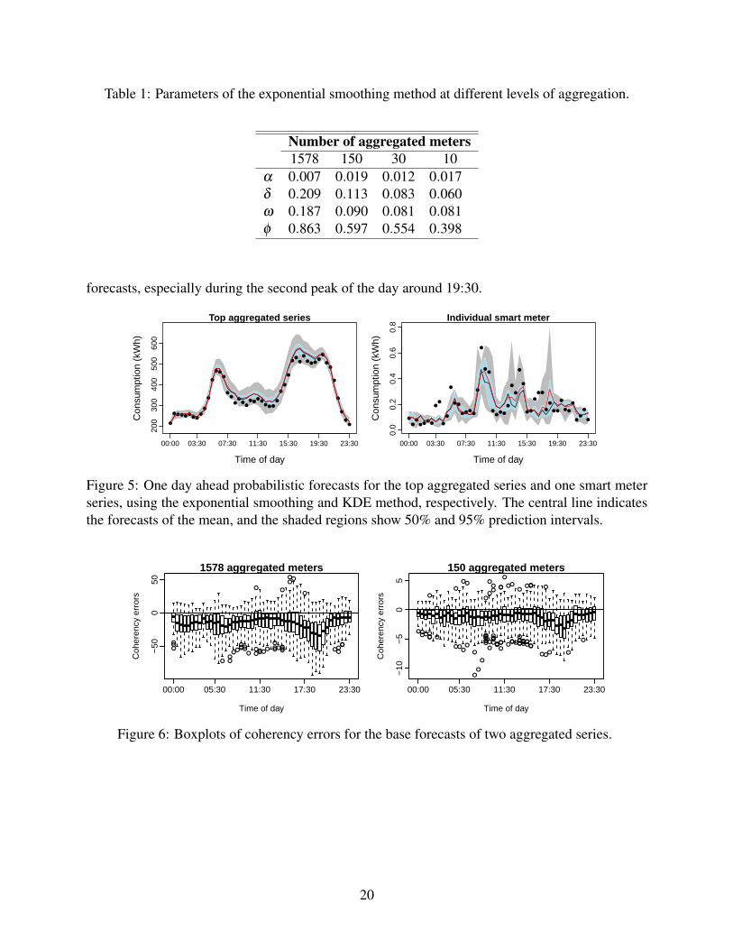
Table 1: Parameters of the exponential smoothing method at different levels of aggregation.

Number of aggregated meters1578 150 30 10

α 0.007 0.019 0.012 0.017δ 0.209 0.113 0.083 0.060ω 0.187 0.090 0.081 0.081φ 0.863 0.597 0.554 0.398

forecasts, especially during the second peak of the day around 19:30.

200

300

400

500

600

Top aggregated series

Time of day

Con

sum

ptio

n (k

Wh)

●

● ● ● ●●

● ●●

●

●

●

● ●

●

●●

●

●●

●

● ●●

●●

● ●

●

●

●

●

●●

●

●

●● ●

●

●

●

●

●

●

●

●

●

00:00 03:30 07:30 11:30 15:30 19:30 23:30

0.0

0.2

0.4

0.6

0.8

Individual smart meter

Time of day

Con

sum

ptio

n (k

Wh)

●

●

●

● ●●

●

●●

●

●

●

● ●

● ● ●●

●

●

●●

●●

● ●

●

●

●

●

●

● ●

●

● ●

●

●

● ●

●

● ●

●

●

●

●

●

00:00 03:30 07:30 11:30 15:30 19:30 23:30

Figure 5: One day ahead probabilistic forecasts for the top aggregated series and one smart meterseries, using the exponential smoothing and KDE method, respectively. The central line indicatesthe forecasts of the mean, and the shaded regions show 50% and 95% prediction intervals.

●●●

● ●●

●●●●●●●

●

●

●●

●●●●

●

●●●

●

●●●

●●

●

●

●●●

●●

−50

050

1578 aggregated meters

Time of day

Coh

eren

cy e

rror

s

00:00 05:30 11:30 17:30 23:30

●●●●

●

●●● ●

●

●●

●

●

●

●

●

●●

●

●

●●●

●●

●

●●

●

●

●

●

●

●

●

●●

●

●

●●●

●●

●●

●

●

●

●

●

●●●●

●

●●●

●●●●●

●

●●●

●●

●●

●●

●

● ●

●

−10

−5

05

150 aggregated meters

Time of day

Coh

eren

cy e

rror

s

00:00 05:30 11:30 17:30 23:30

●●

●

●●●

●●

●●●

●●

●

●

●

●

●

●

●●●●●

●

●●●●●

●

●

●

● ●

●

●●

●

●●

●

−2

−1

01

30 aggregated meters

Time of day

Coh

eren

cy e

rror

s

00:00 05:30 11:30 17:30 23:30

●●

●● ●

●●

●

●

●

●

●

●

●

●

●

●●●

●

●

●

●●

●

●●

●●

●●

●

●●● ●

●

●

●

●

●

●● ●

●● ●

●

●●

−1.

5−

0.5

0.5

10 aggregated meters

Time of day

Coh

eren

cy e

rror

s

00:00 05:30 11:30 17:30 23:30

Figure 6: Boxplots of coherency errors for the base forecasts of two aggregated series.

20

6 Empirical Study of Smart Meter Data

In this section, we empirically evaluate mean and probabilistic hierarchical forecasts. We first

describe the evaluation measures that we use, and list the forecasting methods in our study.

6.1 Evaluation measures

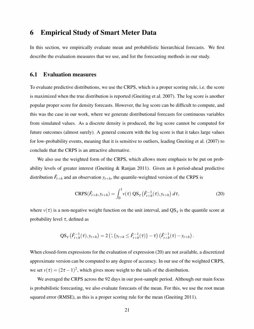
To evaluate predictive distributions, we use the CRPS, which is a proper scoring rule, i.e. the score

is maximized when the true distribution is reported (Gneiting et al. 2007). The log score is another

popular proper score for density forecasts. However, the log score can be difficult to compute, and

this was the case in our work, where we generate distributional forecasts for continuous variables

from simulated values. As a discrete density is produced, the log score cannot be computed for

future outcomes (almost surely). A general concern with the log score is that it takes large values

for low-probability events, meaning that it is sensitive to outliers, leading Gneiting et al. (2007) to

conclude that the CRPS is an attractive alternative.

We also use the weighted form of the CRPS, which allows more emphasis to be put on prob-

ability levels of greater interest (Gneiting & Ranjan 2011). Given an h period-ahead predictive

distribution Ft+h and an observation yt+h, the quantile-weighted version of the CRPS is

CRPS(Ft+h,yt+h) =∫ 1

0v(τ) QSτ

(F−1

t+h(τ),yt+h)

dτ, (20)

where v(τ) is a non-negative weight function on the unit interval, and QSτ is the quantile score at

probability level τ , defined as

QSτ

(F−1

t+h(τ),yt+h)= 2

(1{yt+h ≤ F−1

t+h(τ)}− τ)(

F−1t+h(τ)− yt+h

).

When closed-form expressions for the evaluation of expression (20) are not available, a discretized

approximate version can be computed to any degree of accuracy. In our use of the weighted CRPS,

we set v(τ) = (2τ−1)2, which gives more weight to the tails of the distribution.

We averaged the CRPS across the 92 days in our post-sample period. Although our main focus

is probabilistic forecasting, we also evaluate forecasts of the mean. For this, we use the root mean

squared error (RMSE), as this is a proper scoring rule for the mean (Gneiting 2011).

21

For conciseness, when presenting the results, we report the average of the scores for the peri-

ods of the day split into three eight-hour intervals. For ease of comparison, we present skill scores.

These measure the performance relative to a reference method. In our application, a natural refer-

ence is the base forecasts, which are produced independently for each series in the hierarchy. For

each method, to calculate the skill score, we compute the ratio of the score to that of the base fore-

casts, then subtract this ratio from one, and multiply the result by 100. The skill score, therefore,

conveys the percentage by which a method’s score is superior to the score of the reference method.

6.2 Forecasting methods

For each half-hour of each of the 92 days in our post-sample period, we made predictions from

23:30 of the previous day. This implies 48 different lead times. We computed predictive distribu-

tions using the following seven methods:

1. BASE - We independently produce predictive distributions for each node in the hierarchy.

For each bottom level series, we use the KDE method described in Section 5.1, and for

each aggregate series, we use the exponential smoothing model of Section 5.2. This BASE

method is used as the reference in the calculation of the skill scores.

2. LogN-MinTDiag - Forecasts of the means and variances for each node are computed using

the MinT expressions (8) and (6), respectively. A diagonal covariance matrix WWW h is used

within the method, which led us to label this method MinTDiag in Section 3.2. Forecasts of

the probability distributions are produced by assuming log-normality.

3. LogN-MinTShrink - This is identical to LogN-MinTDiag, except that a shrunken covariance

matrix WWW h is used within the MinT method. We referred to this version of the MinT method

as MinTShrink in Section 3.2.

4. IndepBU-NoMinT - In this bottom-up approach, we compute the aggregate forecasts by

Monte Carlo simulation. Predictive distributions for the aggregates are generated from the

sum of independently sampled values of the predictive distributions, produced by the BASE

method, for the bottom level nodes.

22

5. IndepBU-MinTShrink - This is identical to IndepBU-NoMinT, except that, prior to the

Monte Carlo simulation, the MinTShrink method is used to revise the predictive distribu-

tions produced by the BASE method for the nodes in the bottom level.

6. DepBU-NoMinT - In this bottom-up approach, we impose dependency on the IndepBU-

NoMinT method. Simulation is again used. We compute the aggregate forecasts by sum-

ming permuted independently sampled values from the predictive distributions, produced by

the BASE method, for the bottom level nodes. In other words, we use our algorithm of Sec-

tion 4.5 with Fi,T+h = Fi,T+h in expression (13). Note that the predictive means are equal for

IndepBU-NoMinT and DepBU-NoMinT. This is because they reduce to simple bottom-up

mean forecasts, given by expression (2).

7. DepBU-MinTShrink - This is identical to DepBU-NoMinT, except that, in an initial step,

the MinTShrink method is used to revise the predictive distributions produced by the BASE

method for the nodes in the bottom level.

Although previous literature has not considered any of these seven methods for probabilistic

hierarchical forecasting, we should acknowledge that the BASE method is a simple benchmark,

and that the methods involving MinTDiag and MinTShrink are founded on the work of Wickrama-

suriya et al. (2018), who consider hierarchical forecasting for the mean. The BASE method is typ-

ically neither mean or probabilistically coherent, and the MinT approaches require a distributional

assumption. These issues motivate our use of a bottom-up approach based on Monte Carlo simula-

tion, and we include four of these in our empirical study. While the IndepBU-NoMinT method can

also be considered as a relatively simple benchmark, the IndepBU-MinTShrink method is more

novel and sophisticated, with our aim being to incorporate, within a simple bottom-up approach,

the MinT approach to hierarchical forecasting of the mean. However, it is important to note that

our main methodological contribution is the DepBU-MinTShrink method, which is the algorithm

described in Section 4.5. A simplified version of this is DepBU-NoMinT, which is also new.

6.3 Hierarchical mean forecasting

For different times of the day, Figure 7 presents the RMSE values and Figure 8 shows RMSE

skill scores of different methods for aggregates constructed from different numbers of meters. As

23

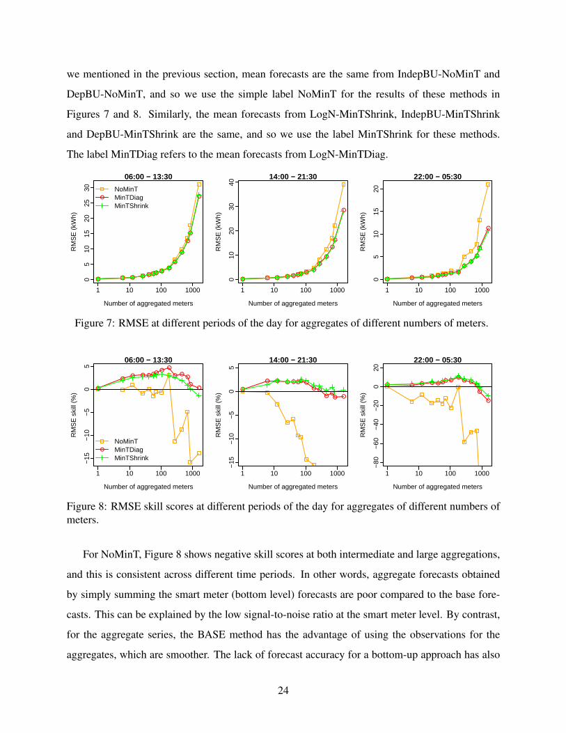
we mentioned in the previous section, mean forecasts are the same from IndepBU-NoMinT and

DepBU-NoMinT, and so we use the simple label NoMinT for the results of these methods in

Figures 7 and 8. Similarly, the mean forecasts from LogN-MinTShrink, IndepBU-MinTShrink

and DepBU-MinTShrink are the same, and so we use the label MinTShrink for these methods.

The label MinTDiag refers to the mean forecasts from LogN-MinTDiag.

05

1015

2025

30

06:00 − 13:30

Number of aggregated meters

RM

SE

(kW

h)

●

●

●

●

●

●●●●●●●●●

1 10 100 1000

●

NoMinTMinTDiagMinTShrink

010

2030

40

14:00 − 21:30

Number of aggregated meters

RM

SE

(kW

h)●

●

●

●

●

●●●●●●●●●

1 10 100 1000

05

1015

20

22:00 − 05:30

Number of aggregated meters

RM

SE

(kW

h)

●

●

●

●●

●●●●●●●●●

1 10 100 1000

Figure 7: RMSE at different periods of the day for aggregates of different numbers of meters.

−15

−10

−5

05

06:00 − 13:30

Number of aggregated meters

RM

SE

ski

ll (%

)

●●

●●●

●●

●●●●●●

●

1 10 100 1000

●

NoMinTMinTDiagMinTShrink

−15

−10

−5

05

14:00 − 21:30

Number of aggregated meters

RM

SE

ski

ll (%

)

●●●

●

●●

●●●●●●●

●

1 10 100 1000

−80

−60

−40

−20

020

22:00 − 05:30

Number of aggregated meters

RM

SE

ski

ll (%

)

●

●

●●●

●●●●●●●●●

1 10 100 1000

Figure 8: RMSE skill scores at different periods of the day for aggregates of different numbers ofmeters.

For NoMinT, Figure 8 shows negative skill scores at both intermediate and large aggregations,

and this is consistent across different time periods. In other words, aggregate forecasts obtained

by simply summing the smart meter (bottom level) forecasts are poor compared to the base fore-

casts. This can be explained by the low signal-to-noise ratio at the smart meter level. By contrast,

for the aggregate series, the BASE method has the advantage of using the observations for the

aggregates, which are smoother. The lack of forecast accuracy for a bottom-up approach has also

24

been observed in many other applications (Hyndman et al. 2011). Although BASE dominates the

NoMinT methods, i.e. IndepBU-NoMinT and DepBU-NoMinT, BASE has the disadvantage of

not producing coherent forecasts, while the bottom-up forecasts are coherent by construction.

In Figure 8, the methods involving MinT perform well. The positive skill scores for these

methods shows that they provide better forecasts than BASE at intermediate aggregations. Recall

that all MinT methods are bottom-up procedures, but with an additional forecast combination step.

The improvement in forecast accuracy, in comparison with the NoMinT methods, shows the effec-

tiveness of including forecast combination in a bottom-up procedure. The relative performance of

MinTDiag and MinTShrink in Figure 8 depends on the time of day, and the level of aggregation.

Recall that, in contrast to MinTShrink, MinTDiag ignores the correlation between the forecast er-

rors at different nodes in the hierarchy. The relative performance of these two methods will depend

on the correlation structure of the base forecast errors, and this will vary across the times of the

day and levels of aggregation. To summarize this section with regard to our proposed method,

DepBU-MinTShrink, the results are encouraging, as it is one of the MinTShrink methods.

6.4 Hierarchical probabilistic forecasting

Figures 7 and 8 showed that IndepBU-NoMinT and DepBU-NoMinT produced poor forecasts of

the mean for the aggregates. This was also the case with the density forecasts from these methods,

which is not surprising, as the accuracy of any density forecast is typically heavily dependent on

the accuracy of the forecast of the location of the density. In view of this, for brevity, in this section,

we focus on the other methods in our discussion of the probabilistic forecasting results.

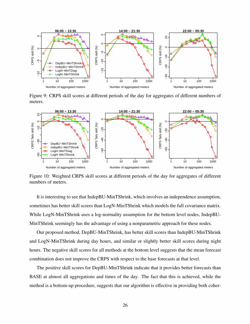
Figures 9 and 10 report the CRPS and weighted CRPS skill scores for DepBU-MinTShrink,

IndepBU-MinTShrink, LogN-MinTDiag and LogN-MinTShrink. In Figure 9, LogN-MinTDiag is

noticeably poorer than LogN-MinTShrink, especially for large aggregations. This contrasts with

the results in Figures 7 and 8 for forecasts of the mean. This is not surprising, as the error corre-

lations directly affect the variance, and hence the predictive distributions, but have only a second-

order effect on the mean. The weighted CRPS results of Figure 10 show an even larger difference

between LogN-MinTDiag and LogN-MinTShrink, indicating that capturing the correlation has a

particularly strong impact on distributional tail accuracy.

25

−10

−5

05

06:00 − 13:30

Number of aggregated meters

CR

PS

ski

ll (%

)

●

●●

●

●

●●

●●●●●●

●

1 10 100 1000

●

DepBU−MinTShrinkIndepBU−MinTShrinkLogN−MinTDiagLogN−MinTShrink

−15

−10

−5

05

14:00 − 21:30

Number of aggregated meters

CR

PS

ski

ll (%

)

●

●●

●

●●

●

●●●●

●●

●

1 10 100 1000

−30

−20

−10

010

22:00 − 05:30

Number of aggregated meters

CR

PS

ski

ll (%

)

●

●

●

●

●

●●●●●

●●

●

●

1 10 100 1000

Figure 9: CRPS skill scores at different periods of the day for aggregates of different numbers ofmeters.

−50

−30

−10

010

06:00 − 13:30

Number of aggregated meters

CR

PS

Tai

ls s

kill

(%)

●

●●

●

●

●

●

●●●

●●

●

●

1 10 100 1000

●

DepBU−MinTShrinkIndepBU−MinTShrinkLogN−MinTDiagLogN−MinTShrink

−60

−40

−20

0

14:00 − 21:30

Number of aggregated meters

CR

PS

Tai

ls s

kill

(%)

●

●●

●

●

●

●

●●●

●●●

●

1 10 100 1000

−60

−40

−20

0

22:00 − 05:30

Number of aggregated meters

CR

PS

Tai

ls s

kill

(%)

●

●

●

●

●●

●●

●●

●

●●

●

1 10 100 1000

Figure 10: Weighted CRPS skill scores at different periods of the day for aggregates of differentnumbers of meters.

It is interesting to see that IndepBU-MinTShrink, which involves an independence assumption,

sometimes has better skill scores than LogN-MinTShrink which models the full covariance matrix.

While LogN-MinTShrink uses a log-normality assumption for the bottom level nodes, IndepBU-

MinTShrink seemingly has the advantage of using a nonparametric approach for these nodes.

Our proposed method, DepBU-MinTShrink, has better skill scores than IndepBU-MinTShrink

and LogN-MinTShrink during day hours, and similar or slightly better skill scores during night

hours. The negative skill scores for all methods at the bottom level suggests that the mean forecast

combination does not improve the CRPS with respect to the base forecasts at that level.

The positive skill scores for DepBU-MinTShrink indicate that it provides better forecasts than

BASE at almost all aggregations and times of the day. The fact that this is achieved, while the

method is a bottom-up procedure, suggests that our algorithm is effective in providing both coher-

26

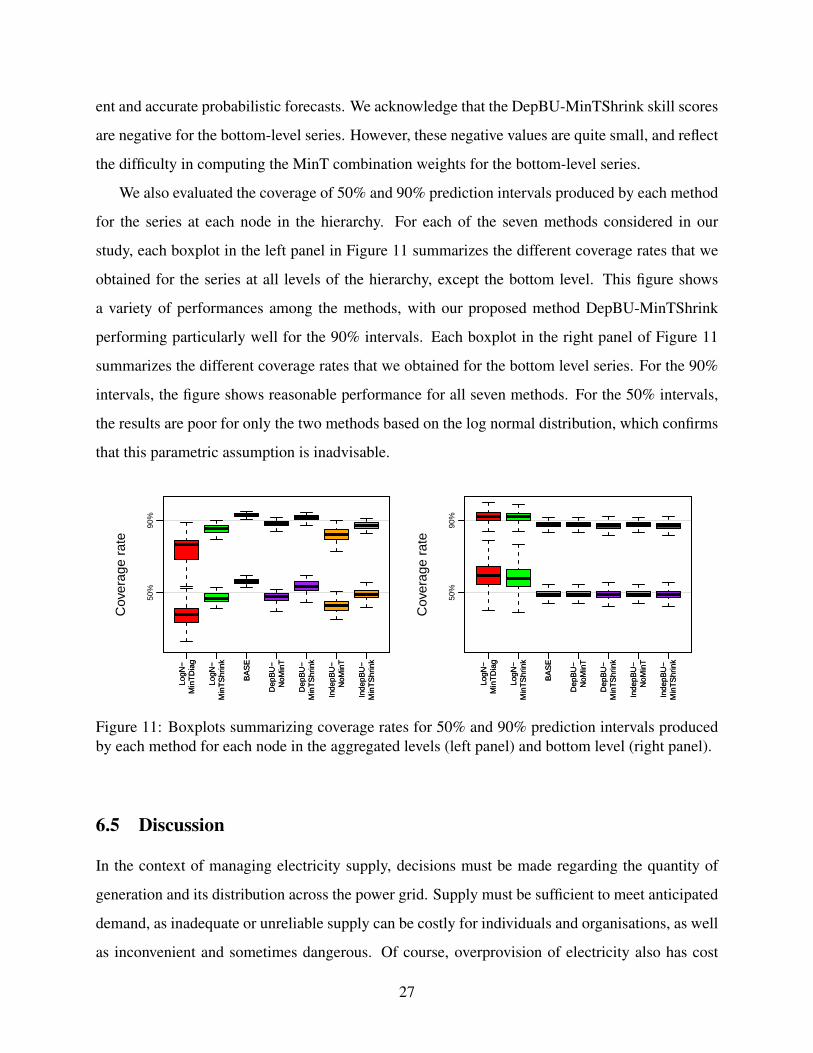
ent and accurate probabilistic forecasts. We acknowledge that the DepBU-MinTShrink skill scores

are negative for the bottom-level series. However, these negative values are quite small, and reflect

the difficulty in computing the MinT combination weights for the bottom-level series.

We also evaluated the coverage of 50% and 90% prediction intervals produced by each method

for the series at each node in the hierarchy. For each of the seven methods considered in our

study, each boxplot in the left panel in Figure 11 summarizes the different coverage rates that we

obtained for the series at all levels of the hierarchy, except the bottom level. This figure shows

a variety of performances among the methods, with our proposed method DepBU-MinTShrink

performing particularly well for the 90% intervals. Each boxplot in the right panel of Figure 11

summarizes the different coverage rates that we obtained for the bottom level series. For the 90%

intervals, the figure shows reasonable performance for all seven methods. For the 50% intervals,

the results are poor for only the two methods based on the log normal distribution, which confirms

that this parametric assumption is inadvisable.

LogN

−

Min

TD

iag

LogN

−

Min

TS

hrin

k

BA

SE

Dep

BU

−

NoM

inT

Dep

BU

−

Min

TS

hrin

k

Inde

pBU

−

NoM

inT

Inde

pBU

−

Min

TS

hrin

k

Cov

erag

e ra

te

50%

90%

LogN

−

Min

TD

iag

LogN

−

Min

TS

hrin

k

BA

SE

Dep

BU

−

NoM

inT

Dep

BU

−

Min

TS

hrin

k

Inde

pBU

−

NoM

inT

Inde

pBU

−

Min

TS

hrin

k

LogN

−

Min

TD

iag

LogN

−

Min

TS

hrin

k

BA

SE

Dep

BU

−

NoM

inT

Dep

BU

−

Min

TS

hrin

k

Inde

pBU

−

NoM

inT

Inde

pBU

−

Min

TS

hrin

k

Cov

erag

e ra

te

50%

90%

LogN

−

Min

TD

iag

LogN

−

Min

TS

hrin

k

BA

SE

Dep

BU

−

NoM

inT

Dep

BU

−

Min

TS

hrin

k

Inde

pBU

−

NoM

inT

Inde

pBU

−

Min

TS

hrin

k

Figure 11: Boxplots summarizing coverage rates for 50% and 90% prediction intervals producedby each method for each node in the aggregated levels (left panel) and bottom level (right panel).

6.5 Discussion

In the context of managing electricity supply, decisions must be made regarding the quantity of

generation and its distribution across the power grid. Supply must be sufficient to meet anticipated

demand, as inadequate or unreliable supply can be costly for individuals and organisations, as well

as inconvenient and sometimes dangerous. Of course, overprovision of electricity also has cost

27

implications, as electricity cannot easily be stored on a large scale, and there are important envi-

ronmental concerns when generation is sourced from fossil fuels. Electricity demand is inherently

uncertain, and particularly so at less aggregated demand points, such as the consumption recorded

by residential smart meters, as shown in Figure 2. This uncertainty must be taken into considera-

tion when making supply decisions. In other words, probabilistic forecasts for demand at different

points in the power grid are required since they are essential for optimal decision making (Gneiting

& Katzfuss 2014).

As we discussed with respect to Figure 1, it is natural to view the forecasting of electricity

consumption as a hierarchical forecasting problem. The literature in this area has emphasised the

need for forecast coherency. For our application, this is important from a practical perspective, be-

cause decisions regarding the allocation of electricity at one level of the hierarchy rely on sufficient

electricity being provided from the previous level, and this is unlikely if forecasts at the different

levels are not coherent in a statistical sense. An important feature of our method is that it delivers

a hierarchy of probabilistic forecasts that are coherent. By contrast, Figure 6 shows that this is not

a feature of the base forecasting method.

Coherency can be ensured by using a simple bottom-up forecasting method. However, as our

results in Figure 8 show, this approach provides poor forecast accuracy. Base forecasting is far

more accurate, but it is a practical concern that it does not deliver a set of coherent forecasts for

the hierarchy. Our results in Figures 8 and 10 show that our method successfully builds on the

base forecasts by, in a sense, drawing on the ‘wisdom of the crowd’ of forecasts in the hierar-

chy, to deliver improvements in accuracy, while ensuring coherency. Our results also confirm the

importance of avoiding distributional assumptions, which is important for an electricity demand

hierarchy, where highly disaggregated data is typically more positively skewed than aggregated

data. In terms of computational feasibility, any forecasting approach for this application only has

practical relevance if it is scalable, and this was an important feature in the design of our method.

7 Empirical Study of Simulated Data

In this section, we describe a simulation study that we used to analyze how well each hierarchical

forecasting method captures the true distribution under different data conditions. Our simulation

28

design was based on the study in Section 3.2 of Wickramasuriya et al. (2018), who focused on

point forecasting. We adjusted and extendeded that study to probabilistic forecasting.

Our hierarchy consisted of three levels with 126 series in total. More specifically, 100 series at

the bottom level were aggregated in groups of four for the next level, resulting in 25 series. These

25 series were then aggregated to obtain the top level series.

Each series in each group of four was generated from an ARMA(p,q) process with p and q set

equal to 0, 1 and 2, with equal probability. The parameters were chosen randomly from a uniform

distribution over a space well within the stationary and invertible parameter space (see Table 1

in Wickramasuriya et al. 2018). For the random error terms, we used a Gaussian distribution 1.

To induce dependences between the series, we used a four-dimensional Gaussian copula with a

covariance matrix that allowed a strongly positive error dependency among the series within each

group of four bottom level series, but only moderately positive dependency between bottom level

series from different groups.

The bottom level series were first generated, and then summed to obtain the series for the levels

above. We considered both a short and long time series, namely T = 500 and T = 10,000. We

focused on one-step-ahead prediction for period T +1. For the purpose of evaluating distributional

forecasts, we obtained a sample of 1000 simulated values from the true distribution, for period

T +1, at each node of the hierarchy. To achieve this, we proceeded by simulating a value from each

bottom level series for period T +1, and then summing appropriately to obtain the value for each

series in the levels above. Doing this 1000 times delivered the sample of simulated values from the

true distribution in period T +1 at each node.

For each series in the hierarchy, the base forecasts were generated using an ARMA model

fitted using the automated algorithm of Hyndman & Khandakar (2008), which is implemented

in the f orecast package for R (Hyndman 2017). The one-step ahead predictive distributions were

generated by bootstrapping the residuals. We felt that inaccuracy in the base forecasts at the bottom

level might limit insight regarding the hierarchical probabilistic forecasting methods. In view of

this, we ran our simulation experiments in two different ways. First, for the base forecasts at the

bottom level, we used the true lag order and parameters from the ARMA data generating processes.

1We also considered a Student’t distribution with six degrees of freedom, but this did not lead to notably moreinsight. The details are given in Appendix A in the supplementary materials.

29

We could not repeat this for the series in the higher levels, as the parameters of the true data

generating processes for these levels is unknown. Our second run of the simulation experiments

used estimated ARMA parameters to produce forecasts for each series in the hierarchy.

To produce probabilistic forecasts for the full hierarchy, we implemented the seven methods

listed in Section 6.2. For the two methods that included a log normal distribution in Section 6.2,

we instead used a Gaussian distribution in our simulation study. We refer to these two methods as

Norm-MinTDiag and Norm-MinTShrink.

For each series, given a sample from the predictive distribution and a sample from the true

distribution, we performed a two-sample Kolmogorov–Smirnov (KS) test, for which the null hy-

pothesis is that the two samples are drawn from the same distribution. We repeated this for each

of 1000 simulated hierarchies. Each panel in Figures 12a and 12b gives boxplots of the resulting

p-values for the case where we used true ARMA parameters to produce the bottom level forecasts.

Under the null hypothesis, the p-values are uniformly distributed. Uniformity is, therefore, the

ideal result. In each figure, the first of the four panels is for the top-level series, the second panel

is for one series in the second level, and the third panel is for one series in the bottom level.

By comparing the third panels of Figures 12a and 12b, i.e. the bottom level of the hierarchy,

we can see that all methods capture the true distribution better when the time series length is

increased from T = 500 to T = 10,000. Note that the bottom level forecasts from IndepBU-

NoMinT and DepBU-NoMinT are equal to the base forecasts. The first and second panels show

that for the upper levels of the hierarchy, regardless of the time series length, performance was

poor for the three methods that do not model the dependences between the series in the bottom

level, i.e. Norm-MinTDiag, IndepBU-NoMinT and IndepBU-MinTShrink. In Figure 12b, the

impressive performance of Norm-MinTShrink can be explained by the method’s distributional

assumption being the same as the error of the data generating process. The DepBU-NoMinT

method and our proposed DepBU-MinTShrink method involve no distributional assumption, as

they are nonparametric, and so it is encouraging that they also performed well.

As we indicated previously, the results of Figures 12a and 12b correspond to the case where we

used true ARMA parameters to produce the bottom level forecasts. Figures 13a and 13b are the

analogous results for the case where we used estimated ARMA parameters to produce forecasts

for each series in the hierarchy. These results are similar to those in Figures 12a and 12b, with the

30

●●●●●●●●●●●●●●●●●●●●●●●●●●●●●●●●●●●●●●●●●●●●●●●●●●●●●●●●●●●●●●●●●●●●●●●●●●●●●●●●●●●●●●●●●●●●●●●●●●●●●●●●●●●●●●●●●●●●●●●●●●●●●●●●●●●●●●●●●●●●●●●●●●●●●●●●●●●●●●●●●●●●●●●●●●●●●●●●●●●●●●●●

●●

●

●

●

●

●

●●

●

●●●

●

●

●●

●

●●●●●●●●●●

●

●●●●●●●●●●●●●●●●●

●

●●●

●

●●●●●●●●●●

●

●●●●●●

●

●●

●●

●●●●●●●

●

●

●

●

●●●●●

●

●

●●

●

●●●●●●●●●

●●●●●●●●●●●●●●

●

●●

●●

●

●●●●●●

●●●● ●

●

●●●●

●

●●●●●●●

●

●●●●●●●●●●

●

●●

●●●●●●●●●●●

●

●●●●

●●

●●●

●●●●●●

●

●

●●●●●●●●●●●●●●●●●

●●●

●●●

●

●●●●●●

●●●●●●●

●●●●●●

●

●●●●●●●

●

●●●●

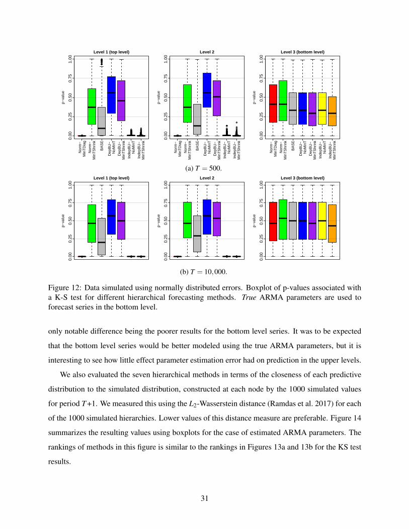
Nor

m−

M

inT

Dia

g

Nor

m−

M

inT

Shr

ink

BA

SE

Dep

BU

−

NoM

inT

Dep

BU

−

Min

TS

hrin

k

Inde

pBU

−

NoM

inT

Inde

pBU

−

Min

TS

hrin

k

Level 1 (top level)

p−va

lue

0.00

0.25

0.50

0.75

1.00

●●●●●●●●●●●●●●●●●●●●●●●●●●●●●●●●●●●●●●●●●●●●●●●●●●●●●●●●●●●●●●●●●●●●●●●●●●●●●●●●●●●●●●●●●●●●●●●●●●●●●●●●●●●●●●●●●●●●●●●●●●●●●●●●●●●●●●●●●●●●●●●●●●●●●●●●●●●●●●●●●●●●●

●●●

●

●●●●●●

●

●●●●●●●●●●●●●

●●●●●

●

●

●

●●

●

●

●●

●

●●

●

●●●

●

●●●●●

●●

●

●

●

●

●●●●

●

●●●●●●●●

●●●●●

●

●●●●●●●●●●●●●●

●

●●●●●● ●

●●●●

●

●●●●●●

●

●●●●●●●●●●●●●●●●●●●●●●●

●

●

●

●●●●●

●

●

●

●●●

●●●

●

●●●●

●

●●

●●●●●

●

●●

●

●●

●

●●●●●●

●●

●●

●

●

●

●●●●

●

●●●●●

●●●●●●●●●●●●●●●●

●

●●●●●

Nor

m−

M

inT

Dia

g

Nor

m−

M

inT

Shr

ink

BA

SE

Dep

BU

−

NoM

inT

Dep

BU

−

Min

TS

hrin

k

Inde

pBU

−

NoM

inT

Inde

pBU

−

Min

TS

hrin

k

Level 2

p−va

lue

0.00

0.25

0.50

0.75

1.00

Nor

m−

M

inT

Dia

g

Nor

m−

M

inT

Shr

ink

BA

SE

Dep

BU

−

NoM

inT

Dep

BU

−

Min

TS

hrin

k

Inde

pBU

−

NoM

inT

Inde

pBU

−

Min

TS

hrin

k

Level 3 (bottom level)

p−va

lue

0.00

0.25

0.50

0.75

1.00

(a) T = 500.

●●●●●●●●●●●●●●●●●●●●●●●●●●●●●●●●●●●●●●●●●●●●●●●●●●●●●●●●●●●●●●●●●●●●●●●●●●●●●●●●●●●●●●●●●●●●●●●●●●●●●●●●●●●●●●●●●●●●●●●●●●●●●●●●●●●●●●●●●●●●●●●●●●●●●●●●●●●●●●●●●●●●●●●●●●●●●●●●●●●●●●●● ●●●●●●●●●●●●●●●●●●●●●●●●●●●●●●●●●●●●●●●●●●●●●●●●●●●●●●●●●●●●●●●●●●●●●●●●●●●●●●●●●●●●●●●●●●●●●●●●●●●●●●●●●●●●●●●●●●●●●●●●●●●●●●●●●●●●●●●●●●●●●●●●●●●●●●●● ●●●●●●●●●●●●●●●●●●●●●●●●●●●●●●●●●●●●●●●●●●●●●●●●●●●●●●●●●●●●●●●●●●●●●●●●●●●●●●●●●●●●●●●●●●●●●●●●●●●●●●●●●●●●●●●●●●●●●●●●●●●●●●●●●●●●●●●●●●●●●●●●●●●

Level 1 (top level)

p−va

lue

0.00

0.25

0.50

0.75

1.00

●●●●●●●●●●●●●●●●●●●●●●●●●●●●●●●●●●●●●●●●●●●●●●●●●●●●●●●●●●●●●●●●●●●●●●●●●●●●●●●●●●●●●●●●●●●●●●●●●●●●●●●●●●●●●●●●●●●●●●●●●●●●●●●●●●●●●●●●●●●●●●●●●●●●●●●●●●●●●●●●●●●●●●●●●●●●●●●●●●● ●●●●●●●●●●●●●●●●●●●●●●●●●●●●●●●●●●●●●●●●●●●●●●●●●●●●●●●●●●●●●●●●●●●●●●●●●●●●●●●●●●●●●●●●●●●●●●●●●●●●●●●●●●●●●●●●●●●●●●●●●●●●●●●●●●●●●●●●●●●● ●●●●●●●●●●●●●●●●●●●●●●●●●●●●●●●●●●●●●●●●●●●●●●●●●●●●●●●●●●●●●●●●●●●●●●●●●●●●●●●●●●●●●●●●●●●●●●●●●●●●●●●●●●●●●●●●●●●●●●●●●●●●●●●●●●●●●●●●●●●●●●●●●

Level 2

p−va

lue

0.00

0.25

0.50

0.75

1.00

Level 3 (bottom level)

p−va

lue

0.00

0.25

0.50

0.75

1.00

(b) T = 10,000.

Figure 12: Data simulated using normally distributed errors. Boxplot of p-values associated witha K-S test for different hierarchical forecasting methods. True ARMA parameters are used toforecast series in the bottom level.

only notable difference being the poorer results for the bottom level series. It was to be expected

that the bottom level series would be better modeled using the true ARMA parameters, but it is

interesting to see how little effect parameter estimation error had on prediction in the upper levels.

We also evaluated the seven hierarchical methods in terms of the closeness of each predictive

distribution to the simulated distribution, constructed at each node by the 1000 simulated values

for period T +1. We measured this using the L2-Wasserstein distance (Ramdas et al. 2017) for each

of the 1000 simulated hierarchies. Lower values of this distance measure are preferable. Figure 14

summarizes the resulting values using boxplots for the case of estimated ARMA parameters. The

rankings of methods in this figure is similar to the rankings in Figures 13a and 13b for the KS test

results.

31

●●●●●●●●●●●●●●●●●●●●●●●●●●●●●●●●●●●●●●●●●●●●●●●●●●●●●●●●●●●●●●●●●●●●●●●●●●●●●●●●●●●●●●●●●●●●●●●●●●●●●●●●●●●●●●●●●●●●●●●●●●●●●●●●●●●●●●●●●●●●●●●●●●●●●●●●●●●●●●●●●●●●●●●●●●●●●●●●●●●●●●●●●●●●●●●

●

●

●

●

●

●●

●

●

●

●

●

●

●

●

●

●

●●

●

●

●

●●

●●

●

●

●

●

●

●●

●●●●

●●

●

●

●

●●●●●●●●●●●

●●●●

●●

●

●●●

●

●●●●

●

●

●●●●●●●●●

●●●●

●●

●●●●

●

●●

●

●●●●●●●●●●●●●●●●●

●

●●●●●●

●

●●●●●●●

●

●●●●●●

●

●●●●●●●●

●●

●

●●●

●

●

●

●●●●●●● ●

●●

●●●●●●●●●●●●●●●●●●●●●●●●●●

●

●●●●●●●●●●●●●●●●●●●●●

●

●

●

●●●●●●●●●

●

●●●●

●●●●●●●

●●●●●●●●●●●●●●

●

●●●●●●●●●●

●●●●●●●●●●●●

●

●●●●●

●

●●●●●●●●●●

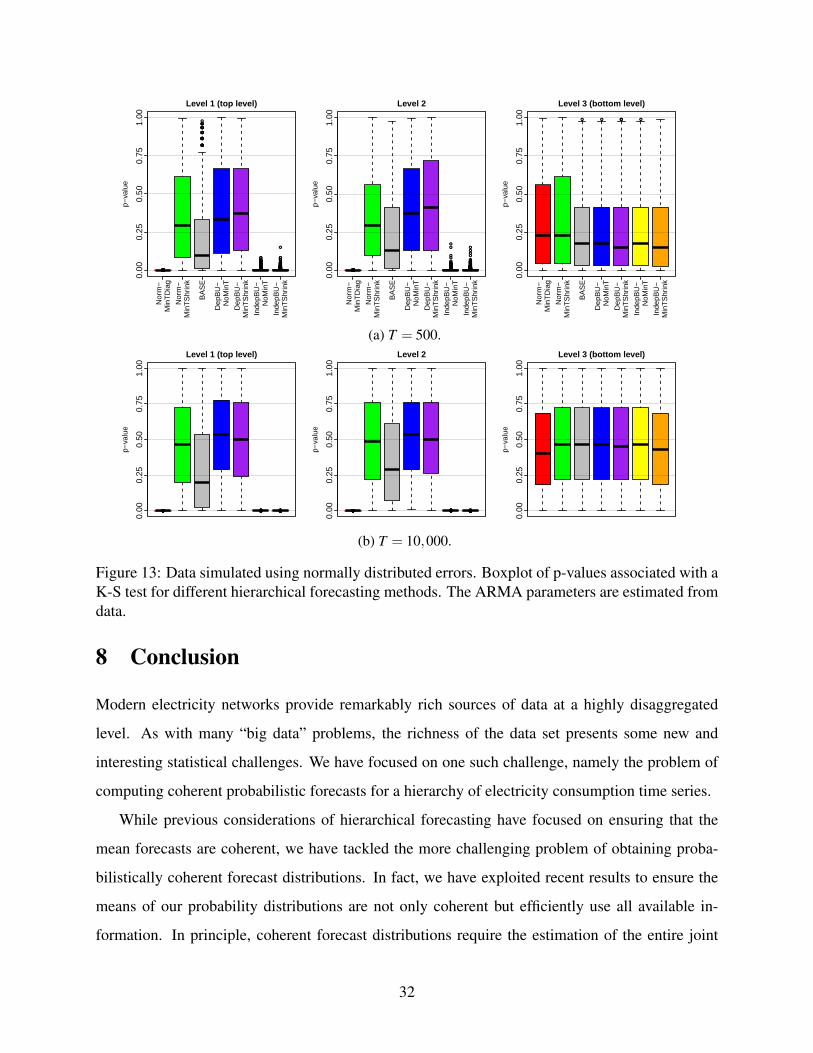
Nor

m−

M

inT

Dia

g

Nor

m−

M

inT

Shr

ink

BA

SE

Dep

BU

−

NoM

inT

Dep

BU

−

Min

TS

hrin

k

Inde

pBU

−

NoM

inT

Inde

pBU

−

Min

TS

hrin

k

Level 1 (top level)

p−va

lue

0.00

0.25

0.50

0.75

1.00

●●●●●●●●●●●●●●●●●●●●●●●●●●●●●●●●●●●●●●●●●●●●●●●●●●●●●●●●●●●●●●●●●●●●●●●●●●●●●●●●●●●●●●●●●●●●●●●●●●●●●●●●●●●●●●●●●●●●●●●●●●●●●●●●●●●●●●●●●●●●●●●●●●●●●●●●●●●●●●●●●●●●●●●●●●●●●●●●●●●●●●●●●●●●●●

●

●●●●●●●●●●●●

●

●●●●●●●●●●●●●

●●

●●●●

●●●●●●

●●●●●●●●

●●●●●●●●●●●●●●●●

●

●●●●●●●

●

●●●●●●●

●●

●

●●●●●●●

●

●

●

●●

●●●●●

●●●●●●●●●●●●●●●●

●

●●●●●●●●●●●●●●●●●●

●

●●●

●

●●●●●●●●

●●●●●●●●●●●●●●

●●●●●●●●●●

●●

●

●●●●

●

●●●●

●

●●●

●

●●●

●●

●●

●

●●●

●

●●●●●●●●

●

●

●●●●●●

●

Nor

m−

M

inT

Dia

g

Nor

m−

M

inT

Shr

ink

BA

SE

Dep

BU

−

NoM

inT

Dep

BU

−

Min

TS

hrin

k

Inde

pBU

−

NoM

inT

Inde

pBU

−

Min

TS

hrin

k

Level 2

p−va

lue

0.00

0.25

0.50

0.75

1.00

● ● ●● ●

Nor

m−

M

inT

Dia

g

Nor

m−

M

inT

Shr

ink

BA

SE

Dep

BU

−

NoM

inT

Dep

BU

−

Min

TS

hrin

k

Inde

pBU

−

NoM

inT

Inde

pBU

−

Min

TS

hrin

k

Level 3 (bottom level)

p−va

lue

0.00

0.25

0.50

0.75

1.00

(a) T = 500.

●●●●●●●●●●●●●●●●●●●●●●●●●●●●●●●●●●●●●●●●●●●●●●●●●●●●●●●●●●●●●●●●●●●●●●●●●●●●●●●●●●●●●●●●●●●●●●●●●●●●●●●●●●●●●●●●●●●●●●●●●●●●●●●●●●●●●●●●●●●●●●●●●●●●●●●●●●●●●●●●●●●●●●●●●●●●●●●●●●●●●●●●●●●●●●●●● ●●●●●●●●●●●●●●●●●●●●●●●●●●●●●●●●●●●●●●●●●●●●●●●●●●●●●●●●●●●●●●●●●●●●●●●●●●●●●●●●●●●●●●●●●●●●●●●●●●●●●●●●●●●●●●●●●●●●●●●●●●●●●●●●●●●●●●●●●●●●●●●●●●●●●●●● ●●●●●●●●●●●●●●●●●●●●●●●●●●●●●●●●●●●●●●●●●●●●●●●●●●●●●●●●●●●●●●●●●●●●●●●●●●●●●●●●●●●●●●●●●●●●●●●●●●●●●●●●●●●●●●●●●●●●●●●●●●●●●●●●●●●●●●●●●

Level 1 (top level)

p−va

lue

0.00

0.25

0.50

0.75

1.00

●●●●●●●●●●●●●●●●●●●●●●●●●●●●●●●●●●●●●●●●●●●●●●●●●●●●●●●●●●●●●●●●●●●●●●●●●●●●●●●●●●●●●●●●●●●●●●●●●●●●●●●●●●●●●●●●●●●●●●●●●●●●●●●●●●●●●●●●●●●●●●●●●●●●●●●●●●●●●●●●●●●●●●●●●●●●●●●●●●●●●●●●● ●●●●●●●●●●●●●●●●●●●●●●●●●●●●●●●●●●●●●●●●●●●●●●●●●●●●●●●●●●●●●●●●●●●●●●●●●●●●●●●●●●●●●●●●●●●●●●●●●●●●●●●●●●●●●●●●●●●●●●●●●●●●●●●●●●●●●●●●●●●●●●●●●●● ●●●●●●●●●●●●●●●●●●●●●●●●●●●●●●●●●●●●●●●●●●●●●●●●●●●●●●●●●●●●●●●●●●●●●●●●●●●●●●●●●●●●●●●●●●●●●●●●●●●●●●●●●●●●●●●●●●●●●●●●●●●●●●●●●●●●●●●●●●●●●●●●●●●●●●●●●●

Level 2

p−va

lue

0.00

0.25

0.50

0.75

1.00

Level 3 (bottom level)

p−va

lue

0.00

0.25

0.50

0.75

1.00

(b) T = 10,000.

Figure 13: Data simulated using normally distributed errors. Boxplot of p-values associated with aK-S test for different hierarchical forecasting methods. The ARMA parameters are estimated fromdata.

8 Conclusion

Modern electricity networks provide remarkably rich sources of data at a highly disaggregated

level. As with many “big data” problems, the richness of the data set presents some new and

interesting statistical challenges. We have focused on one such challenge, namely the problem of

computing coherent probabilistic forecasts for a hierarchy of electricity consumption time series.

While previous considerations of hierarchical forecasting have focused on ensuring that the

mean forecasts are coherent, we have tackled the more challenging problem of obtaining proba-

bilistically coherent forecast distributions. In fact, we have exploited recent results to ensure the

means of our probability distributions are not only coherent but efficiently use all available in-

formation. In principle, coherent forecast distributions require the estimation of the entire joint

32

Nor

m−

M

inT

Dia

g

Nor

m−

M

inT

Shr

ink

BA

SE

Dep

BU

−

NoM

inT

Dep

BU

−

Min

TS

hrin

k

Inde

pBU

−

NoM

inT

Inde

pBU

−

Min

TS

hrin

k

−1

0

1

2

3

4

Level 1 (top level)

2−W

asse

rste

in d

ista

nce

(log

scal

e)

Nor

m−

M

inT

Dia

g

Nor

m−

M

inT

Shr

ink

BA

SE

Dep

BU

−

NoM

inT

Dep

BU

−

Min

TS

hrin

k

Inde

pBU

−

NoM

inT

Inde

pBU

−

Min

TS

hrin

k

−4

−3

−2

−1

0

1

Level 2

2−W

asse

rste

in d

ista

nce

(log

scal

e)

Nor

m−

M

inT

Dia

g

Nor

m−

M

inT

Shr

ink

BA

SE

Dep

BU

−

NoM

inT

Dep

BU

−

Min

TS

hrin

k

Inde

pBU

−

NoM

inT

Inde

pBU

−

Min

TS

hrin

k

−6

−5

−4

−3

−2

Level 3 (bottom level)

2−W

asse

rste

in d

ista

nce

(log

scal

e)

(a) T = 500.

−1

0

1

2

3

4

Level 1 (top level)

2−W

asse

rste

in d

ista

nce

(log

scal

e)

−5

−4

−3

−2

−1

0

Level 2

2−W

asse

rste

in d

ista

nce

(log

scal

e)

−7

−6

−5

−4

Level 3 (bottom level)

2−W

asse

rste

in d

ista

nce

(log

scal

e)

(b) T = 10,000.

Figure 14: Data simulated using normally distributed errors. Boxplot of L2-Wasserstein distancescomputed between a sample from the true data generating process and a sample from the predictivedistribution for 1000 simulations. The ARMA parameters are estimated from data.

distribution of all the bottom-level time series. To circumvent this problem, we exploit the hier-

archical structure of the data, allowing us to reduce the problem to smaller sub-problems, each of

which is computationally tractable. Another feature of our approach is that we make no assump-

tions about the underlying distributions, using conditional KDE for the smart meter time series, and

using fast time series models that handle the multiple seasonal patterns observed in the aggregated

data. For our smart meter data, overall, the best performing method involves mean forecast com-

bination using a shrinkage estimator for the covariance matrix of the one-step forecast errors, and

our copula-based approach for computing the predictive distributions of all nodes in the hierarchy.

Although we have focused on electricity demand, our work is applicable to other contexts,

such as sales product hierarchies, or tourist numbers in geographical hierarchies. In addition to

considering such applications, we are interested in adapting our approach for count data, and de-

33

veloping an approach based on Bayesian hierarchical modeling, which would have the appeal of

the Bayesian framework, although the need for parametric assumptions is likely. In this paper, non-

parametric approaches have featured heavily with KDE for the base forecasting of the bottom level

series, an empirical distribution used with the exponential smoothing forecasts, and an empirical

copula employed within our algorithm. These methods are reasonable for situations, such as ours,

where quite long time series are available. However, for short series, these approaches are likely

to be improved with the use of parametric methods, and this would be an interesting area of future

research. In terms of a parametric method for base forecasting, it would be interesting to consider

dynamic factor models or sparse vector autoregressive models (see Bessa et al. (2015); Dowell &

Pinson (2016)), although dimensionality is likely to be a challenge. It would also be interesting

to consider applications with significant missing observations. Missing observations can be par-

ticularly challenging for hierarchical forecasting when the series have missing values in different

periods, leading to an accumulation of missing values in the aggregate series. A further area of

interest is the use of our approach within a procedure for optimizing the hierarchy architecture (see

Misiti et al. (2010)).

Acknowledgments

We are very grateful to the Editor, an associate editor and three referees for providing very useful

comments on the paper.

ReferencesAECOM (2011), Energy demand research project: Final analysis, Technical report, AECOM House, Hert-

fordshire, UK.AECOM Building Engineering (2014), ‘Energy demand research project: Early smart meter trials, 2007-

2010’, http://doi.org/10.5255/UKDA-SN-7591-1.Arbenz, P., Hummel, C. & Mainik, G. (2012), ‘Copula based hierarchical risk aggregation through sample

reordering’, Insurance, Mathematics & Economics 51(1), 122–133.Arora, S. & Taylor, J. W. (2016), ‘Forecasting electricity smart meter data using conditional kernel density

estimation’, Omega 59, Part A, 47–59.Ben Taieb, Huser, R., Hyndman, R. J. & Genton, M. G. (2016), ‘Forecasting uncertainty in electricity smart

meter data by boosting additive quantile regression’, IEEE Transactions on Smart Grid 7(5), 2448–2455.

34

Berrocal, V. J., Raftery, A. E., Gneiting, T. & Steed, R. C. (2010), ‘Probabilistic weather forecasting forwinter road maintenance’, Journal of the American Statistical Association 105(490), 522–537.

Bessa, R. J., Trindade, A. & Miranda, V. (2015), ‘Spatial-Temporal solar power forecasting for smart grids’,IEEE Transactions on Industrial Informatics 11(1), 232–241.

Borenstein, S. & Bushnell, J. (2015), ‘The US electricity industry after 20 years of restructuring’, Annual

Review of Economics 7(1), 437–463.Borges, C. E., Penya, Y. K. & Fernandez, I. (2013), ‘Evaluating combined load forecasting in large power

systems and smart grids’, IEEE Transactions on Industrial Informatics 9(3), 1570–1577.Cabrera, B. L. & Schulz, F. (2017), ‘Forecasting generalized quantiles of electricity demand: A functional

data approach’, Journal of the American Statistical Association 112(517), 127–136.Cho, H., Goude, Y., Brossat, X. & Yao, Q. (2013), ‘Modeling and forecasting daily electricity load curves:

A hybrid approach’, Journal of the American Statistical Association 108(501), 7–21.Cottet, R. & Smith, M. (2003), ‘Bayesian modeling and forecasting of intraday electricity load’, Journal of

the American Statistical Association 98(464), 839–849.De Livera, A. M., Hyndman, R. J. & Snyder, R. (2011), ‘Forecasting time series with complex seasonal

patterns using exponential smoothing’, Journal of the American Statistical Association 106(496), 1513–1527.

Dowell, J. & Pinson, P. (2016), ‘Very-Short-Term probabilistic wind power forecasts by sparse vector au-toregression’, IEEE Transactions on Smart Grid 7(2), 763–770.

Gijbels, I. & Herrmann, K. (2014), ‘On the distribution of sums of random variables with copula-induceddependence’, Insurance, Mathematics & Economics 59, 27–44.

Gneiting, T. (2011), ‘Making and evaluating point forecasts’, Journal of the American Statistical Associa-

tion 106(494), 746–762.Gneiting, T., Balabdaoui, F. & Raftery, A. E. (2007), ‘Probabilistic forecasts, calibration and sharpness’,

Journal of the Royal Statistical Society. Series B, Statistical methodology 69(2), 243–268.Gneiting, T. & Katzfuss, M. (2014), ‘Probabilistic forecasting’, Annual Review of Statistics and Its Appli-

cation 1(1), 125–151.Gneiting, T. & Ranjan, R. (2011), ‘Comparing density forecasts using threshold- and Quantile-Weighted

scoring rules’, Journal of Business & Economic Statistics 29(3), 411–422.Grimit, E. P., Gneiting, T., Berrocal, V. J. & Johnson, N. A. (2006), ‘The continuous ranked probability

score for circular variables and its application to mesoscale forecast ensemble verification’, Quarterly

Journal of the Royal Meteorological Society 132(621C), 2925–2942.Haben, S., Ward, J., Vukadinovic Greetham, D., Singleton, C. & Grindrod, P. (2014), ‘A new error measure

for forecasts of household-level, high resolution electrical energy consumption’, International Journal of

Forecasting 30(2), 246–256.Hall, P., Racine, J. & Li, Q. (2004), ‘Cross-Validation and the estimation of conditional probability densi-

ties’, Journal of the American Statistical Association 99(468), 1015–1026.Hong, T., Pinson, P., Fan, S., Zareipour, H., Troccoli, A. & Hyndman, R. J. (2016), ‘Probabilistic energy

forecasting: Global energy forecasting competition 2014 and beyond’, International Journal of Forecast-

35

ing 32(3), 896–913.Hyndman, R. J. (2017), ‘forecast: Forecasting functions for time series and linear models’.Hyndman, R. J., Ahmed, R. A., Athanasopoulos, G. & Shang, H. L. (2011), ‘Optimal combination forecasts

for hierarchical time series’, Computational statistics & data analysis 55(9), 2579–2589.Hyndman, R. J. & Khandakar, Y. (2008), ‘Automatic time series for forecasting: the forecast package for

R’, Journal of Statistical Software 27(3), 1–22.Hyndman, R. J., Lee, A. J. & Wang, E. (2016), ‘Fast computation of reconciled forecasts for hierarchical

and grouped time series’, Computational Statistics & Data Analysis 97, 16–32.Iman, R. L. & Conover, W. J. (1982), ‘A distribution-free approach to inducing rank correlation among

input variables’, Communications in Statistics - Simulation and Computation 11(3), 311–334.Jeon, J. & Taylor, J. W. (2012), ‘Using conditional kernel density estimation for wind power density fore-

casting’, Journal of the American Statistical Association 107(497), 66–79.Kremer, M., Siemsen, E. & Thomas, D. J. (2016), ‘The sum and its parts: Judgmental hierarchical forecast-

ing’, Management Science 62(9), 2745–2764.Mainik, G. (2015), ‘Risk aggregation with empirical margins: Latin hypercubes, empirical copulas, and

convergence of sum distributions’, Journal of Multivariate Analysis 141, 197–216.Mirowski, P., Chen, S., Ho, T. K. & Yu, C.-N. (2014), ‘Demand forecasting in smart grids’, Bell Labs

Technical Journal 18(4), 135–158.Misiti, M., Misiti, Y., Oppenheim, G. & Poggi, J.-M. (2010), ‘Optimized clusters for disaggregated elec-

tricity load forecasting’, REVSTAT– Statistical Journal 8(2), 105–124.Nelsen, R. B. (2007), An introduction to copulas, Springer Science & Business Media.Patton, A. J. (2006), ‘Modelling asymmetric exchange rate dependence’, International Economic Review

47(2), 527–556.Ramchurn, S. D., Vytelingum, P., Rogers, A. & Jennings, N. R. (2012), ‘Putting the ’smarts’ into the smart

grid: a grand challenge for artificial intelligence’, Communications of the ACM 55(4), 86–97.Ramdas, A., Trillos, N. G. & Cuturi, M. (2017), ‘On wasserstein Two-Sample testing and related families

of nonparametric tests’, Entropy 19(2), 47.Ruschendorf, L. (2009), ‘On the distributional transform, sklar’s theorem, and the empirical copula pro-

cess’, Journal of Statistical Planning and Inference 139(11), 3921–3927.Schafer, J. & Strimmer, K. (2005), ‘A shrinkage approach to large-scale covariance matrix estimation and

implications for functional genomics’, Statistical Applications in Genetics and Molecular Biology 4, 32.Schefzik, R., Thorarinsdottir, T. L. & Gneiting, T. (2013), ‘Uncertainty quantification in complex simu-

lation models using ensemble copula coupling’, Statistical science: a review journal of the Institute of

Mathematical Statistics 28(4), 616–640.Sklar, M. (1959), Fonctions de repartition a n dimensions et leurs marges, Universite Paris 8.Smith, M., Min, A., Almeida, C. & Czado, C. (2010), ‘Modeling longitudinal data using a Pair-Copula

decomposition of serial dependence’, Journal of the American Statistical Association 105(492), 1467–1479.

Sun, X., Luh, P. B., Cheung, K. W., Guan, W., Michel, L. D., Venkata, S. S. & Miller, M. T. (2016), ‘An

36

efficient approach to Short-Term load forecasting at the distribution level’, IEEE Transactions on Power

Systems 31(4), 2526–2537.Taylor, J. W. (2010), ‘Exponentially weighted methods for forecasting intraday time series with multiple

seasonal cycles’, International Journal of Forecasting 26(4), 627–646.Taylor, J. W. & Buizza, R. (2002), ‘Neural network load forecasting with weather ensemble predictions’,

IEEE Transactions on Power Systems 17(3), 626–632.Taylor, J. W. & McSharry, P. (2012), Univariate methods for Short-Term load forecasting, in M. El-Hawary,

ed., ‘Advances in Electric Power and Energy; Power Systems Engineering, Power Engineering Series ofIEEE Press’, Wiley.

van Erven, T. & Cugliari, J. (2015), Game-Theoretically optimal reconciliation of contemporaneous hierar-chical time series forecasts, in ‘Modeling and Stochastic Learning for Forecasting in High Dimensions’,Lecture Notes in Statistics, Springer International Publishing, pp. 297–317.

Wickramasuriya, S. L., Athanasopoulos, G. & Hyndman, R. J. (2018), ‘Optimal forecast reconciliation forhierarchical and grouped time series through trace minimization’, Journal of the American Statistical

Association pp. 1–45.

37