PROBABILISTIC MODEL-BASED DYNAMIC ARCHITECTURE ...

Under review as a conference paper at ICLR 2019

PROBABILISTIC MODEL-BASED DYNAMICARCHITECTURE SEARCH

Anonymous authorsPaper under double-blind review

ABSTRACT

The architecture search methods for convolutional neural networks (CNNs) haveshown promising results. These methods require significant computational re-sources, as they repeat the neural network training many times to evaluate andsearch the architectures. Developing the computationally efficient architecturesearch method is an important research topic. In this paper, we assume that thestructure parameters of CNNs are categorical variables, such as types and connec-tivities of layers, and they are regarded as the learnable parameters. Introducingthe multivariate categorical distribution as the underlying distribution for the struc-ture parameters, we formulate a differentiable loss for the training task, where thetraining of the weights and the optimization of the parameters of the distributionfor the structure parameters are coupled. They are trained using the stochasticgradient descent, leading to the optimization of the structure parameters withina single training. We apply the proposed method to search the architecture fortwo computer vision tasks: image classification and inpainting. The experimentalresults show that the proposed architecture search method is fast and can achievecomparable performance to the existing methods.

1 INTRODUCTION

Convolutional neural networks (CNNs) make remarkable progress in various computer vision tasks.As researchers have developed deeper architectures and new components to improve performance,the architecture of CNNs is becoming complicated. Since numerous modules exist to construct CNNarchitectures, designing the appropriate CNN architecture for a target problem is critical. However,finding a better combination of basic modules for CNNs, e.g., convolutional and pooling layers,requires tremendous trial and error.

In this context, the methods for designing deep neural network architectures are actively proposed.Most existing methods treat the structure parameters, such as the type of layer and the connectivity,as hyper-parameters and optimize them by reinforcement learning (Zoph & Le, 2017) or evolu-tionary algorithms (Real et al., 2017; Suganuma et al., 2017). These methods search for a betterarchitecture that maximizes the performance for validation data in the hyper-parameter optimizationmanner, i.e., they need neural network training for an architecture evaluation. This approach has suc-ceeded in finding the state-of-the-art CNN architectures; however, it is computationally inefficientin general. Reducing the computational cost of the architecture search is critical for practical usage.Several pieces of research have focused on reducing the computational cost of architecture search(Liu et al., 2018b; Pham et al., 2018) by reusing the trained weights on different architectures andsimultaneously optimizing the weights and the structure parameters. Another practical requirementis that the architecture search methods have fewer hyper-parameters to reduce the total effort of thearchitecture search process.

This work aims to develop an efficient architecture search method with fewer hyper-parameters. Asneural network architectures can be represented by a sequence of categorical variables (Pham et al.,2018; Suganuma et al., 2017; 2018), we consider the neural networks consist of categorical vari-ables of the structure parameters and continuous variables of the weights. Introducing multivariatecategorical distribution as the underlying distribution for the structure parameters, we formulate anexpected loss function under the distribution that is differentiable with respect to (w.r.t.) both theweights and the parameters of the distribution. We iteratively update the weights and the param-

1


eters of the distribution to the gradient steps within a single training, realizing a computationallyefficient architecture search. The idea of the proposed method is based on Shirakawa et al. (2018),which instantiates the algorithm using the multivariate Bernoulli distribution and has proofed theconcept on the simple neural network structure optimization. We extend their work and make it pos-sible to search flexible architectures. We call the algorithm proposed in this paper the probabilisticmodel-based dynamic architecture search (PDAS). The straightforward probabilistic modeling ofthe architectures adopted in this work leads to the simple update rule of the parameters of the distri-bution, which relates to the stochastic natural gradient method (Ollivier et al., 2017). Moreover, weestablish the parameter-adaptive architecture search method by injecting the learning rate adaptationmechanism of the stochastic natural gradient proposed in Nishida et al. (2018).

We apply the PDAS to search the architectures for two computer vision tasks: image classificationand inpainting. The experimental results show that the PDAS is fast and can achieve comparableperformance to the existing architecture search methods on both tasks.

The contribution of this paper is as follows: (1) we derive the algorithm for categorical distributionand make it possible to apply the framework proposed in Shirakawa et al. (2018) to the architecturesearch spaces represented by categorical variables. To the best of our knowledge, the natural gradi-ent of categorical distribution has not been introduced in the context of stochastic natural gradientmethods. (2) we show that PDAS, which has fewer hyper-parameters than efficient neural archi-tecture search (ENAS) (Pham et al., 2018), is fast and can reach state-of-the-art performance. Theintrinsic hyper-parameters of PDAS are the sample size and the learning rate, but the learning ratecan be adaptive.

2 PROBABILISTIC MODEL-BASED DYNAMIC ARCHITECTURE SEARCH

Formulation: Following Shirakawa et al. (2018), we consider the neural network φ(W,M) hav-ing two different sets of parameters: the connection weights W ∈ W and the structure parametersM ∈ M. We assume that the weights are real-valued and differentiable for loss function; however,the structure parameters can be discrete, i.e., the loss function is not differentiable w.r.t. these param-eters. Our original objective is minimizing the loss L(W,M) =

∫D l(z,W,M)p(z)dz, whereD and

l(z,W,M) indicate the dataset and the loss function value of a datum z, respectively. Introducinga family of probability distributions pθ(M) of M parametrized by a real-valued vector θ ∈ Θ, weformulate a minimization of the expected loss under pθ(M), namely

G(W, θ) =

∫ML(W,M)pθ(M)dM , (1)

where dM is a reference measure onM. That is, we try to minimize the loss L(W,M) indirectlyby minimizing G(W, θ). This formulation is inspired from the recently-introduced black-box opti-mization framework called Information Geometric Optimization (Ollivier et al., 2017). The point is,one can choose the family of probability distributions so that G is differentiable w.r.t. both W andθ. It allows us to employ a gradient descent to optimize W and θ simultaneously within a singletraining process.

We apply a stochastic gradient descent to minimize G onW×Θ equipped with the Fisher metric onΘ. That is, we take the vanilla gradient w.r.t.W and the natural gradient (Amari, 1998) w.r.t. θ.Theycan be approximated by Monte-Carlo using λ samples drawn from pθ(M) and mini-batch lossL(W,M) ≈ L̄(W,M) = N̄−1

∑N̄k l(zk,W,M) with mini-batch size N̄ . Then, we get

∇WG(W, θ) ≈ 1

λ

λ∑n=1

∇W L̄(W,Mn) , (2)

∇̃θG(W, θ) ≈ 1

λ

λ∑n=1

L̄(W,Mn)∇̃θ ln pθ(Mn) , (3)

where ∇̃θ ln pθ(M) = F−1(θ)∇θ ln pθ(M) is the natural gradient of the log-likelihood ln pθ(M),and F (θ) is the Fisher information matrix of pθ(M). Shirakawa et al. (2018) proposed the frame-work that simultaneously optimizes both W and θ by using approximated gradients of (2) and (3),and they instantiated the algorithm using the multivariate Bernoulli distribution. In other words,

2


they used the binary vector to select the network components, such as the unit, layer, and type ofactivation.

Categorical Parameters: In this paper, we consider categorical parameters as they can representmore flexible network architecture than binary parameters. We extend the previous work by intro-ducing the multivariate categorical distribution as pθ(M). We denote theD-dimensional categoricalvariables by h = (h1, . . . , hD)T and the number of categories for the i-th variable by Ki (> 1). Letus introduce the one-hot representation of hi, denoted as mi ∈ {0, 1}Ki , where the entries of mi

are all zero but for the hi-th entry, which is one. Our structure parameter vector M is then writtenas M = (m1, . . . ,mD)T.

We introduce the multivariate categorical distribution pθ as the underlying distribution forM , whoseprobability mass is pθ(M) =

∏Di=1

∏Ki

j=1 (θij)mij , where θij ∈ [0, 1] represents the probability of

mij to be 1 and must satisfy∑Ki

j=1 θij = 1. The natural gradient of the log-likelihood for the abovedistribution is given by ∇̃θ ln pθ(M) = M − θ, since the natural gradient of the log-likelihood foran exponential family with sufficient statistics T (M) with the expectation parameterization θ =

E[T (M)] is known to be ∇̃θ ln pθ(M) = T (M) − θ and the above parametrized distribution is anexponential family with the expectation parameterization. See Appendix A for details.

With this natural gradient of log-likelihood, we get the update rule of θ as follows:

θ(t+1) = θ(t) +ηθλ

λ∑n=1

un(Mn − θ(t)) , (4)

where ηθ is the learning rate. As done in Ollivier et al. (2017); Shirakawa et al. (2018), we trans-form the loss value L̄(W,Mn) into the utility un to make the update invariant for the scale of theobjective values. We use the following ranking-based utility transformation: un = 1 for best dλ/4esamples, un = −1 for worst dλ/4e samples, and un = 0 otherwise. The update rule (4) is thegeneralization of the case for Bernoulli distribution and ensures

∑Ki

j=1 θ(t+1)ij = 1. The parameters

of the distribution are initialized by θ(0)ij = K−1

i if we have no prior knowledge. Moreover, we setthe lower bound for θij as θmin

i = (D(Ki − 1))−1 to leave open the possibility of generating allvalues (see Appendix B for details).

Learning Rate Adaptation for Stochastic Natural Gradient Ascent: The update formula (4) re-quires two hyper-parameters, namely the learning rate ηθ and the number λ of Monte-Carlo samples.For Bernoulli distribution, Shirakawa et al. (2018) set λ = 2 and ηθ = D−1, the former of which isthe minimum requirement to use a ranking-based utility transformation. As Bernoulli distribution isa special case of the categorical distribution with Ki = 2 for all i, the learning rate setting may begeneralized as ηθ =

(∑Di (Ki − 1)

)−1. However, as is not difficult to imagine, an adequate value

for ηθ depends heavily on problem characteristic and stage of optimization. Nishida et al. (2018)proposed to adapt ηθ so as to keep the signal-to-noise ratio of successive parameter updates. It hasbeen shown that the adaptive learning rate typically speeds up the convergence of the parameter vec-tors in the case of Bernoulli distributions. The adaptation mechanism can be applied to an arbitraryexponential family with expectation parameterization, which includes our categorical distribution.We employ this learning rate adaptation in our experiments. See Appendix C for details. From thepreliminary experiment in the classification task, we confirmed that the learning rate adaptation im-proves the quality and stability of the architecture search. In the learning rate adaptation, the samplesize λ is fixed to two. From the viewpoint of stochastic approximation theory, the small learningrate has a similar effect of the large sample size. Therefore, even if the sample size equals two, wecan optimize the distribution parameters properly with the appropriate small learning rate. In fact,we observed that the learning rate decreases by the learning rate adaptation mechanism.

Overall Algorithm: The overall algorithm of PDAS is displayed in Algorithm 1. We calculatethe gradients of W and θ using different mini-batches from a dataset. ENAS (Pham et al., 2018)and differentiable architecture search (DARTS) (Liu et al., 2018b), the methods for optimizing thestructure parameters within a single training, use different datasets for the weight and structureparameter optimizations as well. Following these studies, we split the training dataset into halves

3


Algorithm 1 PDAS with learning rate adaptation

Require: training data D = {DW ,Dθ}1: Initialize the weight and distribution parameters as W (0) and θ(0) and the parameters used in

the learning rate adaptation2: for t = 0 · · ·T do3: Sample M1 and M2 independently from pθ(t)4: Compute (2) using M1, M2, and a mini-batch from DW5: Update W (t) by a SGD method6: Update θ(t) by (4) using M1, M2, and a mini-batch from Dθ with updated W7: Update η(t)

θ by the learning rate adaptation mechanism (See Appendix C for details)8: end for9: Get the structure parameters as M∗ = argmaxM pθ(T )(M)

10: Re-train the weights using the fixed architecture represented by M∗

as D = {DW ,Dθ}. The gradients (2) and (3) are calculated using mini-batches from DW and Dθ,respectively, and the parameter updates are performed alternately. As each dataset is sampled fromthe original one, the losses of mini-batch samples from both datasets approximate the original lossof all of the data if the dataset size is sufficiently large. Therefore, even if we use split datasets, wecan view that the losses in the equations of (2) and (3) approximate the original loss.1 Note thatwe do not need the back-propagation for calculating (3). Namely, the computational cost of the θupdate is less than that of W .

After the optimization of W and θ, we can get the most likely structure parameters as M∗ =argmaxM pθ(M), which is obtained trivially for the multivariate categorical distribution. Given theoptimized structure parameters M∗, we re-train the neural network represented by M∗ with initial-ized weights. In the re-training stage, we can exclude the redundant weights (the weight parametersin the unused layer modules) and no longer need to update them. Re-training the obtained archi-tecture is a commonly used technique (Brock et al., 2018; Liu et al., 2018b; Pham et al., 2018) toimprove final performance. We have experimentally observed that the re-training of W can improvethe predictive performance.

3 RELATED WORK

The ordinary architecture search methods (Real et al., 2017; Suganuma et al., 2017; Zoph & Le,2017) for deep neural networks repeat the following steps: the architecture generation, the weighttraining, and the architecture evaluation. Since the weight training of deep neural networks is time-consuming, the overall process requires a tremendous computational cost. Several techniques areintroduced to reduce the training cost, such as inheriting the trained weights to the next candidate ar-chitectures (Real et al., 2017) and stopping the weight training based on the performance prediction(Baker et al., 2018). In contrast, our method is computationally more efficient than these approachesbecause it only needs the training twice (including the re-training).

The existing methods similar to our method are SMASH (Brock et al., 2018) and ENAS (Phamet al., 2018). SMASH randomly samples an architecture in memory-bank representation and deter-mines its weights by a meta-network called HyperNet. Instead of training the weights in the gener-ated network, the HyperNet is trained through back-propagation. Differently from our method, theprobability distribution of network architectures does not change in SMASH, and it still needs themeta-network design. ENAS is a method based on the neural architecture search (NAS) (Zoph &Le, 2017). NAS defines a recurrent neural network, called the controller, that generates a sequenceof categorical variables representing architecture for the main task and optimizes the controller us-ing the policy gradient method in a hyper-parameter optimization manner. ENAS shares the weightparameters in all generated architectures and optimizes the weights and the controller parametersalternatively.

1We can formulate the update rules with different datasets by starting from different original objectives forthe weight and distribution parameters as done in ENAS.

4


Our method is similar to ENAS from the viewpoint of optimizing both of the weights and distributionparameters in a single training. The main difference between PDAS and ENAS is the probabilisticmodel of architectures, i.e., PDAS uses the categorical distribution, and ENAS uses the recurrentneural network. Since our method uses the categorical distribution, the modeling of architectures isintuitive and simple, and all we need is to design the categorical variables for representing architec-tures. As a result, we do not need to design the architecture of the controller neural network thatis required for ENAS. In addition, the simple modeling of architecture makes it possible to derivethe natural gradient in PDAS. As ENAS uses the LSTM network as the controller, it cannot derivethe analytical natural gradient. Also, our method does not require to design the special operator forarchitecture search, such as crossover and mutation used in the evolutionary algorithms (Real et al.,2017). By injecting the learning adaptation mechanism (Nishida et al., 2018), we can further reducethe effort of the hyper-parameter tuning for PDAS. This property is convenient in practice. In theexperiments, we always use the same hyper-parameter setting for PDAS. Another attractive propertyof PDAS is that the promising architecture is determined easily after the training described before,whereas it is difficult in ENAS.

4 EXPERIMENT AND RESULT

We apply the proposed method, the probabilistic model-based dynamic architecture search (PDAS),to the task of finding better architectures for image classification and inpainting. In the architecturesearch, two research directions exist: developing an efficient search method (Liu et al., 2018b; Phamet al., 2018) and designing a search space (Liu et al., 2018a; Zoph et al., 2018). Since PDAS is asearch framework for neural network architectures, we concentrate on evaluating PDAS in terms ofsearch efficiency: the quality of found architecture and the computational cost. Therefore, the exper-iment adopts the search spaces provided in the previous works, Pham et al. (2018) for classificationand Suganuma et al. (2018) for inpainting. All experiments are run using a single NVIDIA GTX1080Ti GPU, and PDAS is implemented using PyTorch 0.4.1 (Paszke et al., 2017).

4.1 IMAGE CLASSIFICATION

Dataset: We use the CIFAR-10 dataset which consists of 50,000 and 10,000 RGB images of 32× 32, for training and testing. All images are standardized in each channel by subtracting the meanand then dividing by the standard deviation. We adopt the standard data augmentation for eachtraining mini-batch: padding 4 pixels on each side, followed by choosing randomly cropped 32 ×32 images and by performing random horizontal flips on the cropped images. We also apply thecutout (DeVries & Taylor, 2017) to the training data.

Search Space: The search space is based on the one in Pham et al. (2018) and the author’s code2,which consists of models obtained by connecting two motifs (called normal cell and reduction cell)repeatedly. An example of the overall model structure can be found in Appendix D. Each cellconsisted of B (= 5) nodes and receives the outputs of the previous two cells as inputs. Each nodereceives two inputs from previous nodes, applies an operation to each of the inputs, and adds them.Our search space includes 5 operations: identity, 3 × 3 and 5 × 5 separable convolutions (Chollet,2017), and 3 × 3 average and max poolings. The separable convolutions are applied twice in theorder of ReLU-Conv-BatchNorm. We select a node by 4 categorical variables representing 2 outputsof the previous nodes and 2 operations applied to them. Consequently, we treat 4B-dimensionalcategorical variables for each cell. After deciding B nodes, all unused outputs of the nodes areconcatenated as the output of the cell. In the reduction cell, all operations applied to the inputs ofthe cell have a stride of 2. The number of the categorical variables is D = 40, and the dimension ofθ becomes 180.

Training Detail: In the architecture search phase, we optimize W and θ for 200 epochs withmini-batch size of 64. We stack 2 normal cells (N = 2) and set the number of channels at the firstcell to 16. For the purpose of absorbing effect of the dynamic change in architecture, we fix affineparameters of batch normalizations. We use SGD with a momentum of 0.9 to optimize W . Thelearning rate changes from 0.025 to 0 followed the cosine schedule (Loshchilov & Hutter, 2017).

2https://github.com/melodyguan/enas

5

https://github.com/melodyguan/enas


Table 1: Comparison with other architecture search methods on CIFAR-10. The notation “+c/o”indicates the cutout (DeVries & Taylor, 2017). The search cost indicates the GPU days for the ar-chitecture search, i.e., without the re-training cost. The result of the architecture randomly sampledfrom our search space is also listed as RANDOM.

Method Search Cost Params Test Error(GPU days) (M) (%)

NAS (Zoph & Le, 2017) 16.8–22.4K 7.1 4.47EAS (DenseNet) (Cai et al., 2018) 20 10.7 3.44SMASHv2 (Brock et al., 2018) 1.5 16.0 4.03

NASNet-A + c/o (Zoph et al., 2018) 2000 3.3 2.65NAONet + c/o (Luo et al., 2018) 200 128 2.07NAONet-WS (Luo et al., 2018) 0.4 3.7 3.53RENASNet + c/o (Chen et al., 2018) 6.0 3.5 2.98 (±0.08)DARTS first order + c/o (Liu et al., 2018b) 1.5 2.9 2.94DARTS second order + c/o (Liu et al., 2018b) 4 3.4 2.83 (±0.06)ENAS + c/o (Pham et al., 2018) 0.45 4.6 2.89

RANDOM + c/o − 3.21 4.12 (±0.44)PDAS + c/o 0.24 3.20 2.98 (±0.12)

We apply weight decay of 3 × 10−4 and clip the norm of gradient at 5. In the re-training phase,we optimize W for 600 epochs with mini-batch size of 80. We stack 6 normal cells (N = 6) andincrease the number of channels at the first cell so that the model of the obtained architecture M∗has nearly three million weight parameters. In contrast to the architecture search phase, we make allbatch normalizations have learnable affine parameters because the architecture no longer changes.We apply the ScheduledDropPath (Zoph et al., 2018) dropping out each path between nodes, andthe drop path rate linearly increases from 0 to 0.3 during the training. We also add the auxiliaryclassifier (Szegedy et al., 2016) with the weight of 0.4 that is connected from the second reductioncell. The total loss is a weighted sum of the losses of the auxiliary classifier and output layer. Othersettings are the same as the architecture search phase. We conducted the experiment five times andreport the average values.

Result and Discussion: Table 1 shows the comparison with other architecture search methods.Since the search space of the first three methods is different from the one used in PDAS, we shouldnot directly compare the test errors to PDAS. At least, we can say that NAS and EAS require muchmore computational cost than PDAS because they repeat training the model many times to optimizenetwork architecture. Although the search cost of SMASH is reasonable, PDAS is still faster thanSMASH.

The other conventional methods adopt search spaces similar to PDAS.3 Compared with these meth-ods, our method is the fastest and shows a comparable error rate to ENAS, DARTS, and RENASNet.The architecture search of PDAS is realized by optimizing θ using (4), and its computational cost issmall, whereas ENAS updates the controller recurrent network that generates the structure parame-ters. This might be one reason that PDAS is fast. DARTS models the architecture by the mixture ofall possible operations and connections and optimizes the weights and the continuous structure pa-rameters (mixture coefficients) by the gradient-based optimization. In the architecture search phase,DARTS requires to compute all possible operations and connections to calculate the gradient. Incontrast, since PDAS computes the gradient using a few sampled structures, it is computationallymore efficient than DARTS. The error rates of NASNet and NAONet outperform our method, butthey have enormous search costs if they are implemented on a single GPU. We observe PDAS cantake a good balance between the test error rate and search cost. The method denoted RANDOMuses the architecture randomly sampled from our search space. The result shows that PDAS can findthe better architecture in a reasonable computational time by optimizing the structure parameters inthe single training.

3The setting, e.g., types of operations, channel sizes, and the number of normal cells N differs among themethods.

6


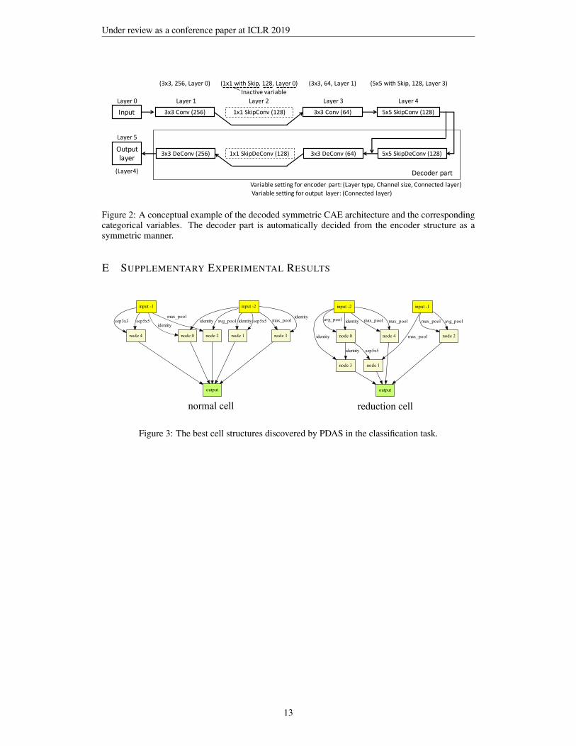
We observed that the value of θ converges to a certain category, and the average value of maxj θij ,implying the convergence of the parameters of the distribution approaches 0.9 at 50th epoch. Thearchitecture of the best model obtained by PDAS appears in Appendix E. We note that PDAS hasfewer hyper-parameters and can be used by only providing the categorical variables for representingthe architecture, whereas, other methods still leave the controller network design or strategy param-eter tuning. As our algorithm is based on the stochastic natural gradient method, we can easily addthe improving techniques, such as the learning rate adaptation used in PDAS.

4.2 INPAINTING

The inpainting task is one of the image restoration tasks, restoring a clean image from a damagedimage with large missing regions (e.g., masks). Suganuma et al. (2018) have shown the potential ofthe architecture search by the evolutionary algorithm for image restoration tasks including inpaint-ing. In this section, we apply the PDAS to the problem of architecture search for inpainting andevaluate its performance. We refer the experimental setting employed in Suganuma et al. (2018).

Dataset and Evaluation Measure: We use three benchmark datasets: the CelebFaces AttributesDataset (CelebA) (Liu et al., 2015), the Stanford Cars Dataset (Cars) (Krause et al., 2013), and theStreet View House Numbers (SVHN) (Netzer et al., 2011). The CelebA is a large-scale human faceimage dataset that contains 202,599 RGB images. We select 101,000 and 2,000 images for trainingand test, respectively, in the same way as Suganuma et al. (2018). All images were cropped toproperly contain the entire face by using the provided bounding boxes and resized to 64× 64 pixels.The Cars is a middle-scale cars image dataset that contains 16,185 RGB images, and it consists of8,144 and 8,041 images for training and testing, respectively. Similar to the CelebA, all imageswere cropped by using the provided bounding boxes and resized to 64 × 64 pixels. The SVHN isa large-scale house-number image dataset that contains 99,289 RGB images without extra trainingdata, and it consists of 73,257 and 26,032 images for training and testing, respectively. The imagesof SVHN were resized to 64 × 64 pixels. All images are normalized by dividing by 255, and weperform data augmentation of random horizontal flipping on the training images.

We test three different masks based on Suganuma et al. (2018); Yeh et al. (2017); a central squareblock mask (Center); a random pixel mask, as 80% of all the pixels were randomly masked (Pixel);and a half image mask, as a randomly selected vertical or horizontal half of the image (Half). Themask was randomly generated for each training mini-batch and each test image.

Following Suganuma et al. (2018), we use two standard evaluation measures: the peak-signal tonoise ratio (PSNR) and the structural similarity index (SSIM) (Wang et al., 2004) to evaluate therestored images. Higher values of these measures indicate a better image restoration.

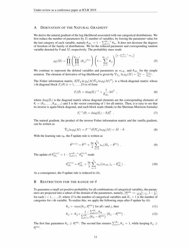
Search Space: The search space we use is based on Suganuma et al. (2018). We employ the CAE,which is similar to the RED-Net (Mao et al., 2016), as a base architecture. The RED-Net consistsof a chain of convolution layers and symmetric deconvolution layers as the encoder and decoderparts, respectively. The encoder and decoder parts perform the same counts of downsampling andupsampling with a stride of 2, and a skip connection between the convolutional layer and the mir-rored deconvolution layer can exist. For simplicity, each layer employs either a skip connectionor a downsampling, and the decoder part is employed in the same manner. In the skip connecteddeconvolution layer, the input feature maps from the encoder part are added to the output of decon-volution operation followed by ReLU. In the other layers, the ReLU activation is performed after theconvolution and deconvolution operations. We prepare six types of layers: the combination of thekernel sizes {1× 1, 3× 3, 5× 5} and the existence of the skip connection. The layers with differentsettings do not share weight parameters.

Since we consider the symmetric CAE, it is enough to represent the encoder part; we only need todetermine the encoder part of the CAE by the categorical variables, and then the decoder part isautomatically decided according to the encoder part. We consider Nc hidden layers and the outputlayer. We encode the type, channel size, and connections of each hidden layer. The kernel sizeand stride of the output deconvolution layer are fixed with 3 × 3 and 1, respectively; however, theconnection is determined by a categorical variable. The numbers of categories for the hidden layertype and the output channel size are 6 and 3, respectively. We select the output channel size of eachlayer from {64, 128, 256}. To ensure the feed-forward architecture and to control the network depth,

7


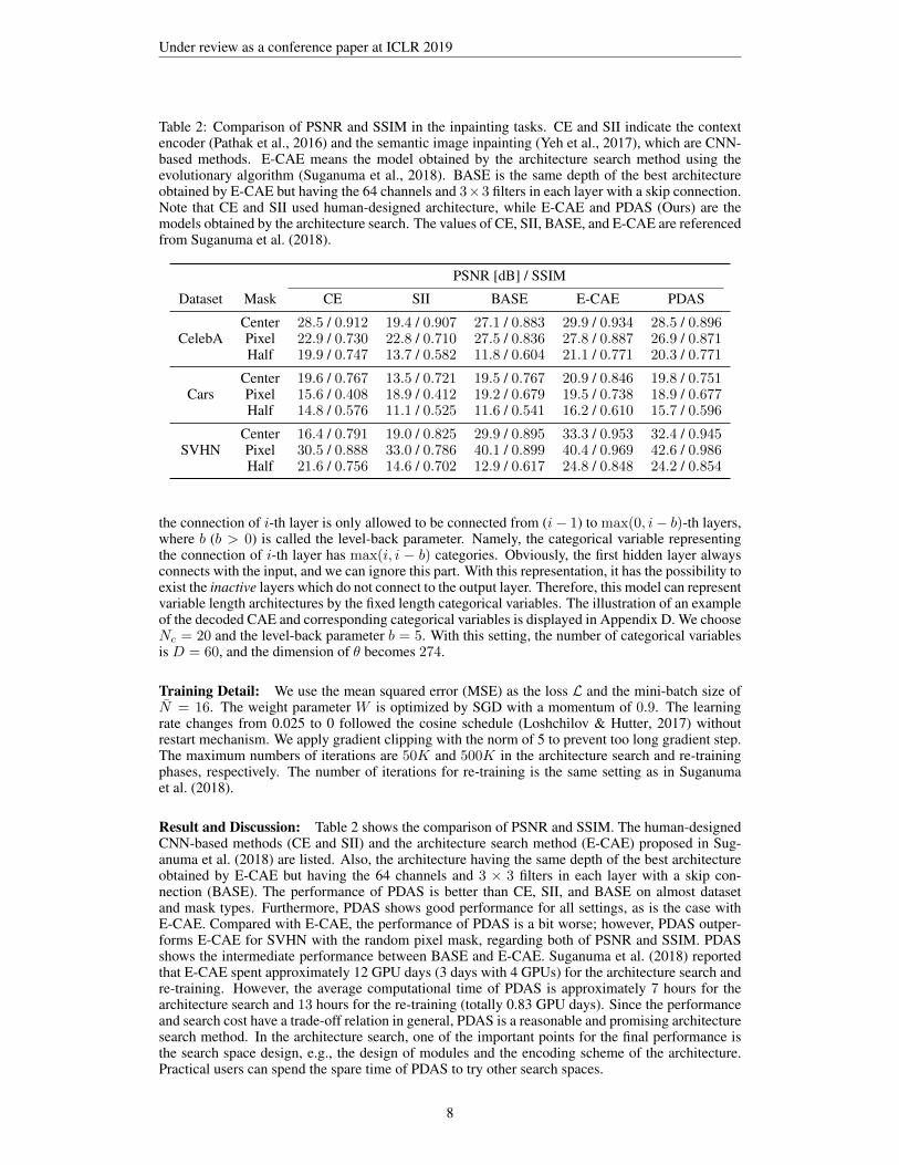
Table 2: Comparison of PSNR and SSIM in the inpainting tasks. CE and SII indicate the contextencoder (Pathak et al., 2016) and the semantic image inpainting (Yeh et al., 2017), which are CNN-based methods. E-CAE means the model obtained by the architecture search method using theevolutionary algorithm (Suganuma et al., 2018). BASE is the same depth of the best architectureobtained by E-CAE but having the 64 channels and 3×3 filters in each layer with a skip connection.Note that CE and SII used human-designed architecture, while E-CAE and PDAS (Ours) are themodels obtained by the architecture search. The values of CE, SII, BASE, and E-CAE are referencedfrom Suganuma et al. (2018).

PSNR [dB] / SSIM

Dataset Mask CE SII BASE E-CAE PDAS

CelebACenter 28.5 / 0.912 19.4 / 0.907 27.1 / 0.883 29.9 / 0.934 28.5 / 0.896Pixel 22.9 / 0.730 22.8 / 0.710 27.5 / 0.836 27.8 / 0.887 26.9 / 0.871Half 19.9 / 0.747 13.7 / 0.582 11.8 / 0.604 21.1 / 0.771 20.3 / 0.771

CarsCenter 19.6 / 0.767 13.5 / 0.721 19.5 / 0.767 20.9 / 0.846 19.8 / 0.751Pixel 15.6 / 0.408 18.9 / 0.412 19.2 / 0.679 19.5 / 0.738 18.9 / 0.677Half 14.8 / 0.576 11.1 / 0.525 11.6 / 0.541 16.2 / 0.610 15.7 / 0.596

SVHNCenter 16.4 / 0.791 19.0 / 0.825 29.9 / 0.895 33.3 / 0.953 32.4 / 0.945Pixel 30.5 / 0.888 33.0 / 0.786 40.1 / 0.899 40.4 / 0.969 42.6 / 0.986Half 21.6 / 0.756 14.6 / 0.702 12.9 / 0.617 24.8 / 0.848 24.2 / 0.854

the connection of i-th layer is only allowed to be connected from (i− 1) to max(0, i− b)-th layers,where b (b > 0) is called the level-back parameter. Namely, the categorical variable representingthe connection of i-th layer has max(i, i − b) categories. Obviously, the first hidden layer alwaysconnects with the input, and we can ignore this part. With this representation, it has the possibility toexist the inactive layers which do not connect to the output layer. Therefore, this model can representvariable length architectures by the fixed length categorical variables. The illustration of an exampleof the decoded CAE and corresponding categorical variables is displayed in Appendix D. We chooseNc = 20 and the level-back parameter b = 5. With this setting, the number of categorical variablesis D = 60, and the dimension of θ becomes 274.

Training Detail: We use the mean squared error (MSE) as the loss L and the mini-batch size ofN̄ = 16. The weight parameter W is optimized by SGD with a momentum of 0.9. The learningrate changes from 0.025 to 0 followed the cosine schedule (Loshchilov & Hutter, 2017) withoutrestart mechanism. We apply gradient clipping with the norm of 5 to prevent too long gradient step.The maximum numbers of iterations are 50K and 500K in the architecture search and re-trainingphases, respectively. The number of iterations for re-training is the same setting as in Suganumaet al. (2018).

Result and Discussion: Table 2 shows the comparison of PSNR and SSIM. The human-designedCNN-based methods (CE and SII) and the architecture search method (E-CAE) proposed in Sug-anuma et al. (2018) are listed. Also, the architecture having the same depth of the best architectureobtained by E-CAE but having the 64 channels and 3 × 3 filters in each layer with a skip con-nection (BASE). The performance of PDAS is better than CE, SII, and BASE on almost datasetand mask types. Furthermore, PDAS shows good performance for all settings, as is the case withE-CAE. Compared with E-CAE, the performance of PDAS is a bit worse; however, PDAS outper-forms E-CAE for SVHN with the random pixel mask, regarding both of PSNR and SSIM. PDASshows the intermediate performance between BASE and E-CAE. Suganuma et al. (2018) reportedthat E-CAE spent approximately 12 GPU days (3 days with 4 GPUs) for the architecture search andre-training. However, the average computational time of PDAS is approximately 7 hours for thearchitecture search and 13 hours for the re-training (totally 0.83 GPU days). Since the performanceand search cost have a trade-off relation in general, PDAS is a reasonable and promising architecturesearch method. In the architecture search, one of the important points for the final performance isthe search space design, e.g., the design of modules and the encoding scheme of the architecture.Practical users can spend the spare time of PDAS to try other search spaces.

8


5 CONCLUSION

We proposed an efficient architecture search method called PDAS that optimizes the parametersof the categorical distribution based on the stochastic natural gradient method during weight train-ing. Our probabilistic modeling of the architecture is straightforward, and the derived algorithmhas fewer hyper-parameters and can incorporate the learning rate adaptation mechanism. The ex-perimental results for the image classification and inpainting tasks have shown that PDAS is fastand achieves comparable performance to the existing methods. In the future, we will apply PDASto other neural network architecture searches (e.g., the recurrent networks) and large-scale datasets(e.g., ImageNet). Regarding the extension of PDAS, the distribution of continuous variables canbe introduced to PDAS; then we will be able to optimize the architecture represented by mixedvariables (e.g., categorical and continuous variables).

REFERENCES

Shun-ichi Amari. Natural Gradient Works Efficiently in Learning. Neural Computation, 10(2):251–276, 1998.

Bowen Baker, Otkrist Gupta, Ramesh Raskar, and Nikhil Naik. Accelerating Neural ArchitectureSearch using Performance Prediction. In International Conference on Learning Representations(ICLR) Workshop, 2018.

Andrew Brock, Theo Lim, J.M. Ritchie, and Nick Weston. SMASH: One-Shot Model Architec-ture Search through HyperNetworks. In International Conference on Learning Representations(ICLR), 2018.

Han Cai, Tianyao Chen, Weinan Zhang, Yong Yu, and Jun Wang. Efficient Architecture Search byNetwork Transformation. In Thirty-Second AAAI Conference on Artificial Intelligence (AAAI),pp. 2787–2794, 2018.

Yukang Chen, Qian Zhang, Chang Huang, Lisen Mu, Gaofeng Meng, and Xinggang Wang. Rein-forced Evolutionary Neural Architecture Search. arXiv preprint:1808.00193, 2018.

Francois Chollet. Xception: Deep Learning with Depthwise Separable Convolutions. In IEEEConference on Computer Vision and Pattern Recognition (CVPR), pp. 1800–1807, 2017.

Terrance DeVries and Graham W. Taylor. Improved Regularization of Convolutional Neural Net-works with Cutout. arXiv preprint:1708.04552, 2017.

Jonathan Krause, Michael Stark, Jia Deng, and Li Fei-Fei. 3D Object Representations for Fine-Grained Categorization. In IEEE International Conference on Computer Vision Workshops (IC-CVW), pp. 554–561, 2013.

Hanxiao Liu, Karen Simonyan, Oriol Vinyals, Chrisantha Fernando, and Koray Kavukcuoglu. Hier-archical Representations for Efficient Architecture Search. In International Conference on Learn-ing Representations (ICLR), 2018a.

Hanxiao Liu, Karen Simonyan, and Yiming Yang. DARTS: Differentiable Architecture Search.arXiv preprint:1806.09055, 2018b.

Ziwei Liu, Ping Luo, Xiaogang Wang, and Xiaoou Tang. Deep Learning Face Attributes in the Wild.In IEEE International Conference on Computer Vision (ICCV), pp. 3730–3738, 2015.

Ilya Loshchilov and Frank Hutter. SGDR: Stochastic Gradient Descent with Warm Restarts. InInternational Conference on Learning Representations (ICLR), 2017.

Renqian Luo, Fei Tian, Tao Qin, Enhong Chen, and Tie-Yan Liu. Neural Architecture Optimization.arXiv preprint:1808.07233, 2018.

Xiao-Jiao Mao, Chunhua Shen, and Yu-Bin Yang. Image Restoration Using Very Deep Convo-lutional Encoder-Decoder Networks with Symmetric Skip Connections. In Advances in NeuralInformation Processing Systems (NIPS), pp. 2802–2810, 2016.

9


Yuval Netzer, Tao Wang, Adam Coates, Alessandro Bissacco, Bo Wu, and Andrew Y. Ng. ReadingDigits in Natural Images with Unsupervised Feature Learning. In Advances in Neural InformationProcessing Systems (NIPS) Workshop on Deep Learning and Unsupervised Feature Learning,2011.

Kouhei Nishida, Hernan Aguirre, Shota Saito, Shinichi Shirakawa, and Youhei Akimoto. Param-eterless Stochastic Natural Gradient Method for Discrete Optimization and its Application toHyper-Parameter Optimization for Neural Network. arXiv preprint:1809.06517, 2018.

Yann Ollivier, Ludovic Arnold, Anne Auger, and Nikolaus Hansen. Information-Geometric Opti-mization Algorithms: A Unifying Picture via Invariance Principles. Journal of Machine LearningResearch, 18(1):564–628, 2017.

Adam Paszke, Gregory Chanan, Zeming Lin, Sam Gross, Edward Yang, Luca Antiga, and ZacharyDevito. Automatic differentiation in PyTorch. In Autodiff Workshop in Thirty-first Conference onNeural Information Processing Systems (NIPS), 2017.

Deepak Pathak, Philipp Krahenbuhl, Jeff Donahue, Trevor Darrell, and Alexei A Efros. ContextEncoders: Feature Learning by Inpainting. In IEEE Conference on Computer Vision and PatternRecognition (CVPR), pp. 2536–2544, 2016.

Hieu Pham, Melody Y. Guan, Barret Zoph, Quoc V. Le, and Jeff Dean. Efficient Neural Architec-ture Search via Parameter Sharing. In The 35th International Conference on Machine Learning(ICML), volume 80, pp. 4095–4104, 2018.

Esteban Real, Sherry Moore, Andrew Selle, Saurabh Saxena, Yutaka Leon Suematsu, Jie Tan,Quoc V. Le, and Alexey Kurakin. Large-Scale Evolution of Image Classifiers. In The 34thInternational Conference on Machine Learning (ICML), volume 70, pp. 2902–2911, 2017.

Shinichi Shirakawa, Yasushi Iwata, and Youhei Akimoto. Dynamic Optimization of Neural Net-work Structures Using Probabilistic Modeling. In Thirty-Second AAAI Conference on ArtificialIntelligence (AAAI), pp. 4074–4082, 2018.

Masanori Suganuma, Shinichi Shirakawa, and Tomoharu Nagao. A Genetic Programming Approachto Designing Convolutional Neural Network Architectures. In The Genetic and EvolutionaryComputation Conference (GECCO), pp. 497–504, 2017.

Masanori Suganuma, Mete Ozay, and Takayuki Okatani. Exploiting the Potential of Standard Con-volutional Autoencoders for Image Restoration by Evolutionary Search. In The 35th InternationalConference on Machine Learning (ICML), volume 80, pp. 4778–4787, 2018.

Christian Szegedy, Vincent Vanhoucke, Sergey Ioffe, Jon Shlens, and Zbigniew Wojna. Rethinkingthe Inception Architecture for Computer Vision. In IEEE Conference on Computer Vision andPattern Recognition (CVPR), pp. 2818–2826, 2016.

Zhou Wang, A.C. Bovik, H.R. Sheikh, and E.P. Simoncelli. Image Quality Assessment: From ErrorVisibility to Structural Similarity. IEEE Transactions on Image Processing, 13(4):600–612, 2004.

Raymond A Yeh, Chen Chen, Teck Yian Lim, Alexander G Schwing, Mark Hasegawa-Johnson, andMinh N Do. Semantic Image Inpainting with Deep Generative Models. In IEEE Conference onComputer Vision and Pattern Recognition (CVPR), pp. 6882–6890, 2017.

Barret Zoph and Quoc V. Le. Neural Architecture Search with Reinforcement Learning. In Interna-tional Conference on Learning Representations (ICLR), 2017.

Barret Zoph, Vijay Vasudevan, Jonathon Shlens, and Quoc V. Le. Learning Transferable Archi-tectures for Scalable Image Recognition. In IEEE Conference on Computer Vision and PatternRecognition (CVPR), pp. 8697–8710, 2018.

10


A DERIVATION OF THE NATURAL GRADIENT

We derive the natural gradient of the log-likelihood associated with our categorical distributions. Wefirst reduce the number of parameters by D, number of variables, by forcing the parameter value forthe last category of each variable, namely θiKi

= 1−∑Ki−1k=1 θik. It does not decrease the degrees

of freedom of the family of distributions. We let the reduced parameter and corresponding randomvariable denoted by θ̄ and M̄ , respectively. The probability mass reads

pθ̄(M̄) =

D∏i=1

Ki−1∏j=1

(θij)mij

1−Ki−1∑j=1

θij

(

1−∑Ki−1

j=1 mij

). (5)

We continue to represent the deleted variables and parameters as miKi and θiKi for the simplenotation. The element of derivative of log-likelihood is given by∇θij ln pθ̄(M̄) =

mij

θij− miKi

θiKi.

The Fisher information matrix, E[∇θ̄ ln pθ̄(M)∇θ̄ ln pθ̄(M)T], is a block-diagonal matrix whosei-th diagonal block Fi(θ̄) (i = 1, . . . , D) is of form

Fi(θ̄) = diag(θ̄i)−1 +

1

θiKi

11T , (6)

where diag(θ̄i) is the diagonal matrix whose diagonal elements are the corresponding elements ofθ̄i = (θi1, . . . , θiKi−1) and 1 is the vector consisting of 1 for all entries. Then, it is easy to see thatits inverse is again block-diagonal, and each block reads (thanks to the Sherman-Morrison formula)

F−1i (θ̄) = diag(θ̄i)− θ̄iθ̄T

i . (7)

The natural gradient, the product of the inverse Fisher information matrix and the vanilla gradient,can be written as

∇̃θ̄ ln pθ̄(M) = F−1(θ̄)∇θ̄ ln pθ̄(M) = M̄ − θ̄ . (8)

With the learning rate ηθ, the θ̄ update rule is written as

θ̄(t+1) = θ̄(t) +ηθλ

λ∑n=1

un(M̄n − θ̄(t)) . (9)

The update of θ(t+1)iKi

= 1−∑Ki−1k=1 θ

(t+1)ik reads

θ(t+1)iKi

= θ(t)iKi

+ηθλ

λ∑n=1

un((miKi)n − θ(t)iKi

) . (10)

As a consequence, the θ update rule is reduced to (4).

B RESTRICTION FOR THE RANGE OF θ

To guarantee a small yet positive probability for all combinations of categorical variables, the param-eters are projected into a subset of the domain of the parameters, namely,

[θmini := 1

D(Ki−1) , 1−1D

]for each i = 1, . . . , D, where D is the number of categorical variables and Ki > 1 is the number ofcategories for i-th variable. To realize this, we apply the following steps after θ update by (4):

θij ← max{θij , θmini } for all i and j, then (11)

θij ← θij+1−

∑Ki

k=1 θik∑Ki

k=1

(θik − θmin

i

) (θij − θmini

). (12)

The first line guarantees θij ≥ θmini . The second line ensures

∑Ki

j=1 θij = 1, while keeping θij ≥θmini .

11


C LEARNING RATE ADAPTATION

The learning rate adaptation proposed by Nishida et al. (2018) is adopted to achieve the parameter-free algorithm and improve the search efficiency. Let s be the accumulation of the parameter updateand γs be its normalization factor, initialized as s(0) = 0 and γ(0)

s = 0, respectively. We denotethe estimated natural gradient in (4) as ∇̃(t)

λ = 1λ

∑λn=1 un(M̄n − θ̄(t)). Note that M and θ are

over-parametrized by the one degree of freedom as mentioned in the natural gradient derivation. Wehence consider M̄ and θ̄ as we considered above. Then, they are updated as

s(t+1) = (1− η(t)θ )s(t) +

√η

(t)θ (2− η(t)

θ )F (θ(t))

12 ∇̃(t)

λ

Tr(F (θ(t))Cov[∇̃(t)λ ])

12

γ(t+1)s = (1− η(t)

θ )2γ(t)s + η

(t)θ (2− η(t)

θ ) .

The estimated natural gradient is scaled w.r.t. the Fisher information matrix and its estimation co-variance. As we can not compute the covaraince matrix analytically, we approximate it by the expec-tation under the assumption that un and Mn are uncorrelated, leading to Tr(F (θ(t))Cov[∇̃(t)

λ ]) =

2−1∑Di=1(Ki − 1), where we used the fact λ = 2, u1 = 1 and u2 = −1. See Nishida et al. (2018)

for its rationale. The learning rate is updated based on the length of s(t+1), namely,

η(t+1)θ = ηmin ∨ η(t)

θ exp(η(t)θ (‖s(t+1)‖2/α− γ(t+1)

s )) ∧ ηmax , (13)

where α = 1.5 is the threshold parameter, ηmin and ηmax are the minimum and maximum learningrate, which are ηmin = 0 and ηmax = (

∑Di=1(Ki − 1))−1/2, respectively. The learning rate is

initialized as η(0)θ = ηmax.

The above procedure requires to compute the square root of F (θ(t)), which is feasible since it ispositive definite. As the Fisher information matrix is a block-diagonal, and each block is of sizeKi−1, a naive computation of F (θ(t))

12 requiresO(

∑Di=1(Ki−1)3). This is usually not expensive

as D � Ki. An alternative way that we employ in this paper is to replace F (θ(t))12 with a tractable

factorization A with F (θ(t)) = AAT. Our choice of A is the block-diagonal matrix whose i-thblock is square, of size Ki − 1, and

Ai = diag(θ̄i)− 1

2 +1

(√θiKi

+ θiKi)1√θ̄i

T, (14)

where√θ̄i is a vector whose j-th element is the square root of θ̄ij . Then, the product of A and

a vector can be computed in O(∑Di=1(Ki − 1)). In our preliminary study we did not obverse any

significant performance difference by this approximation.

D OVERALL MODEL STRUCTURE FOR CLASSIFICATION AND INPAINTINGTASKS

normal

cell

normal

cell

normal

cell

reductioncell

reductioncell

image

softmax

×𝑁

×𝑁

×𝑁

Figure 1: Overall model structure for the classification task in Section 4.1. We optimize the archi-tecture of the normal and reduction cells by PDAS. In the re-training phase, we construct the CNNusing the optimized cell architecture with an increased number of cells N .

12


Layer2Inactivevariable

Input

Outputlayer

Decoderpart

3x3DeConv (256) 1x1SkipDeConv (128) 3x3DeConv (64)

3x3Conv(256) 1x1SkipConv (128) 3x3Conv(64) 5x5SkipConv (128)

5x5SkipDeConv (128)

(3x3,256,Layer0)

Layer0 Layer1 Layer3 Layer4

(1x1withSkip,128,Layer0) (3x3,64,Layer1) (5x5withSkip,128,Layer3)

Layer5

(Layer4)

Variablesettingforencoderpart:(Layertype,Channelsize,Connectedlayer)Variablesettingforoutput layer:(Connectedlayer)

Figure 2: A conceptual example of the decoded symmetric CAE architecture and the correspondingcategorical variables. The decoder part is automatically decided from the encoder structure as asymmetric manner.

E SUPPLEMENTARY EXPERIMENTAL RESULTS

input -2

node 0

identity

node 1

identity sep5x5

node 2

avg_pool

node 3

identitymax_pool

input -1

identity

max_pool

node 4

sep3x3 sep5x5

output

input -2

node 0

avg_pool identity

node 3

identity node 4

max_pool max_pool

input -1

node 1

max_pool node 2

avg_poolmax_pool

sep5x5identity

output

normal cell reduction cell

Figure 3: The best cell structures discovered by PDAS in the classification task.

13

PROBABILISTIC MODEL-BASED DYNAMIC ARCHITECTURE ...

Documents

Transcript of PROBABILISTIC MODEL-BASED DYNAMIC ARCHITECTURE ...