Probabilistic 3D Object RecognitionIlan Shimshoni� and Jean PonceDepartment of Computer Science and Beckman InstituteUniversity of Illinois, Urbana, IL 61801,e-mail: ilans@ie.technion.ac.il.Abstract: A probabilistic 3D object recognition algorithm is presented. In order to guidethe recognition process the probability that match hypotheses between image features andmodel features are correct is computed. A model is developed which uses the probabilisticpeaking e�ect of measured angles and ratios of lengths by tracing iso-angle and iso-ratiocurves on the viewing sphere. The model also accounts for various types of uncertaintyin the input such as incomplete and inexact edge detection. For each match hypothesisthe pose of the object and the pose uncertainty which is due to the uncertainty in vertexposition are recovered. This is used to �nd sets of hypotheses which reinforce each other bymatching features of the same object with compatible uncertainty regions. A probabilisticexpression is used to rank these hypothesis sets. The hypothesis sets with the highest rankare output. The algorithm has been fully implemented, and tested on real images.1 IntroductionOne of the major problems in computer vision is to recognize 3D objects appearing in ascene as instances from a database of models (see [6, 12] for reviews). Several recognitionsystems extract features such as points [21, 26, 27] or lines [4] from the image andmatch them to corresponding features in the database. They then verify each candidatehypothesis using other features in the image and �nally rank the veri�ed hypotheses.�Ilan Shimshoni is now with the Department of Industrial Engineering and Management, Technion,Haifa 32000, Israel. 1

When constructing such a system the major problems to be addressed are: how togenerate match hypotheses, in which order to process the hypotheses, how to verifythem using additional image features, and how to rank the veri�ed hypotheses. In ourapproach, we de�ne a match hypothesis as the matching of a pair of edges or a trihedralcorner (Figure 1) to corresponding feature sets in the model database. The hypothesesare ranked by computing the probability that each one is correct. In order to verify ahypothesis, we compute the pose of the object assuming the match is correct. Otherhypotheses which match other image features to features in the same model should yieldcompatible poses if they correspond to the same object. The pose is transformed from apoint in the pose space to a region of that space when uncertainty in the values measuredin the image is taken into account, and we check whether hypotheses reinforce each otherby testing whether their pose uncertainty regions intersect. We rank sets of hypotheseswhose uncertainty regions intersect by the probability that the match of the whole setis correct, and output a small number of interpretations with the highest ranks. Themain goal of our approach is to �nd a small number of probable interpretations whichcan then be veri�ed by comparing the image to the hypothesized object using standardveri�cation techniques.θ

θ1

2θ

l

l

1

2(a) (b)Figure 1: Image feature sets: (a) two lines in an image l1 and l2; the angle between thelines is �; (b) a corner with three edges emanating from it.2

2 Background and ApproachSince object recognition is one of the main problems in computer vision, a large body ofwork has addressed this problem (see [6, 12] for reviews). Here we focus on a few paperswhose approach is related to ours.Lowe [24] was the �rst to introduce the notion that a partial match of image to modelfeatures yields constraints on the position in the image of other features of the modeldue to rigidity constraints. This was generalized by Gaston and Lozano-P�erez [15] andGrimson and Lozano-P�erez [18] using the term interpretation tree. Classic examples ofthis approach are the algorithm of Ayache and Faugeras [4] for recognition of 2D objects,and the algorithm of Faugeras and Hebert [13] for recognition of 3D objects using rangeimages.In [14, 21], the alignment technique was presented. The algorithm chooses matches ofthe minimal size (three) which enables it to recover the pose of the object [1, 19]. Thusthe position of other points in the image can be estimated and if found help verify thehypothesis. In order to produce reliable recognition systems of this kind the followingproblems have been addressed.� What is the uncertainty in the pose given a possible match of three points in themodel to points in the image whose position is uncertain [17].� In which area around the projected model point should an image point be searched[2, 29].� What size match is required to verify an hypothesis [16].� In which order to test the hypotheses.Probabilistic methods have been developed to rank hypotheses by their likelihood in3

order to refrain from testing all possible match hypotheses. These methods are basedon the probabilistic peaking e�ect [3, 7, 5, 9]. Informally this e�ect can be described asfollows: when randomly choosing a direction from which to observe a pair of adjacentedges, and measuring the ratio of the lengths of the projections of the edges or the anglebetween them in the image, the values measured in the image have a high probability tobe close to the real values measured in the model. In those papers, probability densityfunctions for values measured in the image are estimated by uniformly sampling theviewing sphere. In addition, joint density functions for ratios of lengths and anglesare estimated. The maximum of those density functions are always where the measuredvalues equal the real values measured in the model. Using Bayes's rule, these probabilitiescan be used to estimate the probability that a set of features in the image match a set offeatures in the model. The probabilistic peaking e�ect is exploited in recognition systemspresented in [26, 27, 5, 9, 31].Other researchers take a di�erent approach to recognition. They use statistical [20],and geometric [8, 11, 28] techniques to search the pose space looking for the pose andobject which best describe the image without testing small matches of image and modelfeatures.In this paper, we propose a 3D object recognition algorithm whose input is a set ofstraight lines extracted from a single image by an edge detector. In order to build arobust recognition system we have to account for the fact that the input is not perfect:objects may occlude each other, certain edges may not belong to any instance of anymodel in our model database, and not all edges appearing in the image will be extractedby the edge detector. We explicitly take all these factors into account.We group the lines extracted from the image into two types of feature sets: pairs ofadjacent lines and trihedral corners (Figure 1). For line pairs, we measure the lengthsof edges and the angle between them, and measure only the angles between the lines for4

trihedral corners. Therefore only pairs of edges whose visible part were fully recoveredby the edge detector will yield valid hypothesis where as for trihedral corners that isnot required. We have chosen these two types of features because under the scaledorthographic camera model that we use, they contain the minimal amount of informationrequired to recover the viewing direction, and because the number of image and modelfeatures is linear in the number of vertices in the image and in our model database,reducing the number of hypotheses that have to be tested compared to testing all matchesof vertex triplets in the image to vertex triplets in the model database (as in [21]).In order to speed up the recognition process we rank the match hypotheses using theprobabilistic peaking e�ect, and test them in the corresponding order. When the pose ofthe object is randomly selected, the probabilistic peaking e�ect says that values measuredin the image such as ratios of lengths or angles between edges have a high probability tobe close to the real values measured in the model. For the feature sets we have chosen,we measure for the pair of edges the ratio � of the lengths of the two edges and the angle� between them, and measure two angles �1; �2 for the trihedral corner. We could havecomputed at recognition time for all the hypotheses the probability that the match iscorrect, but in order to speed up the algorithm we partition the (�; �) and (�1; �2) spacesinto rectangles and pre-compute the average probability of hypotheses with measuredvalues within each rectangle. Under the scaled orthographic camera model, the onlycomponent of the pose a�ecting the ratios and angles in the image is the viewing directionwhich is parameterized as a point on the viewing sphere. The area on the viewing spherewhere the measured values are within a rectangle correspond to the required probability.This area is bounded by curves on the viewing sphere where the ratio (iso-ratio curve)or the angle (iso-angle curve) is constant, and equal to the minimum or maximum valuesof each rectangle. We can accurately compute the desired probabilities by computingthe area bounded by these curves. We use the probabilities computed for all model5

feature sets to compute the probability that a match hypothesis is correct given that wemeasured certain values in the image. We compute these probabilities using Bayes's ruleand account in the probabilistic model for self occlusion and imperfect edge data.The model can be extended to incorporate more information about the image (e.g.,the camera position and its relation to the surface on which the objects are placed), byreducing the space of legal poses to stable poses of the objects [22]. This would reducethe number of plausible hypotheses for each feature set considerably.We verify a match hypothesis by computing the pose of the object, assuming thehypothesis is correct. We then try to �nd consistent match hypotheses with close posesthat reinforce the hypothesis. We compute the viewing direction component of the poseof the object by tracing the iso-ratio or iso-angle curves on the viewing sphere whichcorrespond to the ratios and angles measured in the image, and the viewing directionis the intersection point of those curves. The other components of the pose are easilyobtained. This technique works for adjacent edges and trihedral corners, where previouswork developed separate techniques for them [1, 21, 32].Uncertainty in image data causes uncertainty in the pose. So in order to be ableto decide whether two hypotheses reinforce each other, we estimate a region of the posespace which accounts for that uncertainty, so that only hypotheses whose regions intersectreinforce each other.In the �nal stage of the algorithm we use a probabilistic expression to rank matchhypotheses. Analysis of this expression shows that it has the following characteristics:hypotheses which would cause large errors in the measurements in the image are rankedlower than hypotheses with smaller errors, and combinations of feature sets which appearoften in the model database such as rectangular faces are ranked lower than more rarefeature combinations.The rest of the paper is organized as follows. In Section 3 we develop a method6

for computing probability density functions using equations we develop for angles andratios. We use these probabilities for ranking match hypotheses in Section 4. We discusspose estimation and estimate the e�ects of uncertainty on the pose in Section 5. Wepresent our probabilistic expression to rank match hypotheses in Section 6. We showexperimental recognition results in Section 7. Finally, a number of issues raised by ourwork and future research directions are discussed in Section 8.3 Hypothesis Probability ComputationIn this section we compute the probability that a given match hypothesis is correct.We compute probabilities and probability density functions for some observable imagequantity (e.g., the ratio between lengths or an angle) to have a given value when the value(measured in the model) is given. We then extend this technique to joint probabilitiesand probability density functions for two image quantities, and use the results to rankmatch hypotheses.3.1 Iso-ratio and Iso-angle Curve equationsWhen measuring the ratio of line lengths in an image or the angle between lines, wewant to know from what viewing directions this image could be scanned, given a matchbetween the lines and certain edges in the model. Consider two segments l1 and l2 in theimage (Figure 1(a)) which are projections of edges u1 and u2 respectively in the model,such that the ratio between the length of l1 and l2 is � and the angle between them is �.The ratio between the lengths of the projections of u1 and u2 is � for viewing directionsv which satisfy: ju1 � vj � �ju2 � vj = 0: (1)Squaring this equation yields a quadratic equation in v.7

Viewing directions which satisfy:(u1 � v) � (u2 � v)� cos �ju1 � vjju2 � vj = 0; (2)yield an angle � between the projections of u1 and u2. Squaring this equation yields aequation of degree four in v. Note that because only cos2 � appears in the equation, italso accounts for the curves corresponding to �� �; 2�� � and �(�� �). These must beidenti�ed and eliminated.We trace these curves to gain a better understanding of the probabilistic peaking e�ectand use the area bounded by them to calculate probabilities. For tracing the curves weuse an algorithm for tracing algebraic curves [23] which relies on homotopy continuation[25] to �nd all curve singularities and construct a discrete representation of the smoothbranch curves. We add the constraint jvj2 = 1 to the equations derived earlier to insurethat the viewing directions lie on the viewing sphere.For reasons of symmetry, ratios are plotted using a log2 scale. In this way, theratio and its inverse are symmetric around zero (log2 � = � log2(1=�)), and yield similarcurves. We traced curves for values of � with equal intervals on the log2 � scale. Figure2(a) shows curves for values log2 � between �2 and 2 where the the ratio in the modelis 1. Interesting viewing directions are: viewing directions parallel to �u1 where u1 isforeshortened to a point and � is zero, viewing directions parallel to �u2 where u2 isforeshortened to a point and � is in�nite, and viewing directions parallel to �(u1 � u2)where the viewing direction is orthogonal to the plane of u1 and u2 and the ratio is the\real" ratio. For ratios less than the \real" ratio there are two curves which surround theviewing direction parallel to �u1, for ratios greater than the \real" ratio there are twocurves which surround the viewing direction parallel to �u2, and for the ratio equal tothe \real" ratio (log2(�) = 0) the two curves intersect at the viewing directions parallelto �(u1 � u2). 8

For the case when the \real" ratio is not one, consider a viewing direction v whichsatis�es ju1 � vj � �ju2 � vj = 0 (3)for a pair of edges e1 and e2 such that ju1j = ju2j. Consider another pair of edges e01 ande02 such that u01 = �1u1 and u02 = �2u2. Substituting these values into (3) yields:ju01 � vj � ��1�2 ju02 � vj = 0:Thus the perceived ratio at the viewing direction v is ��1=�2 where �1=�2 is the \real"ratio between the lengths of e01 and e02. This linear relationship enables us to concentrateon the case where the edges are of equal length and use this relationship to computevalues for all other pairs of edges. No such relationship exists for angles.

(a)U1

U2

-2.0-1.6-1.2-1.2

-0.8-0.8

-0.4-0.4

0.00.0

0.4

0.8

1.21.62.0

(b)U1

U2

0

15

30

4545

60

7590105120135150165180195210225240255

270285

300330

345

Figure 2: For two lines of equal length with 45� between them: (a) the viewing spherewith iso-ratio curves with log2(�) in [�2; 2]; (b) the viewing sphere with iso-angle curves.In Figure 2(b) we show curves for angles between 0 and 360� where the angle is de�nedas the angle between the projection u1 the projection of u2 in the counterclockwise9

direction and the \real" angle between the two 3D edges is 45�. All the curves startat viewing directions parallel to �u1 and end at viewing directions parallel to �u2.This occurs because at those directions one of the edges has been foreshortened to zerolength and therefore the angle between the two edges is not de�ned. However, by slightlychanging the viewing direction any angle can be obtained. For angles less than the\real" angle, the curves go between u1 and u2 or between �u1 and �u2 starting for 0�from directions in the plane spanned by u1 and u2. At the \real" angle the two curvesintersect like before at the viewing direction orthogonal to the u1,u2 plane. For anglesgreater than the \real" angle the curves go between u1 and �u2 or between �u1 and u2ending for 180� with viewing directions which also lie in the u1,u2 plane. For angles �greater than 180� the curve is the re ection of the curve for 360�� � through the origin.The probabilistic peaking e�ect is clearly demonstrated in this �gure for both ratios andangles. The fraction of the sphere covered by ratios such that �0:4 < log2 � < 0:4 andby 30� < � < 60� is much larger than by other segments of the log2 � and � spaces of thesame size.3.2 Computing Probability Density FunctionsGiven the probability density function (p.d.f.) f , the value of the distribution functionF (a) is the probability that x � a. It is given by:F (a) = Z a�1 f(x)dx:Conversely, f(x) = F 0(x);therefore when one function is given, the other can be computed by integration or di�er-entiation. In our case we �rst compute F (a) for a ratio or an angle and then compute f10

by numerical di�erentiation. The curve for a value of the ratio or an angle a is traced onthe viewing sphere. This curve bounds the part of the viewing sphere for which x � a.The discrete points on the curve bound a polygon whose area is given by the followingformula: area = nXi=1 �i � (n� 2)�;where n is the number of vertices of the polygon, and �i is the spherical angle between twoadjacent edges. A spherical angle is de�ned as the angle between the planes containingthe great circles of the two edges. The area of the whole sphere is 4�, so to obtainprobabilities the result must be divided by 4�. Examples of such curves for various typesof distribution functions computed throughout this paper are shown in Figure 3.

Figure 3: Regions on the viewing sphere whose areas are computed.We can estimate f(x) by:f(x) = lim�!0 F (x+ �)� F (x� �)2� ;using the values computed for F (x + �) and F (x� �).Figure 4(a) shows the probability density function for log2 � for various values of the11

original angle between the edges, where the original ratio is 1. A logarithmic scale isused to re ect the symmetry of the probability density function for ratios.

(a) |

-2.0|

-1.5|

-1.0|

-0.5|

0.0|

0.5|

1.0|

1.5|

2.0

|0.0

|2.0

|4.0

|6.0

|8.0

|10.0

log (ρ)

Pro

babi

lity

Den

sity

(b) |0

|30

|60

|90

|120

|150

|180

|0.00

|0.02

|0.04

|0.06|0.08

|0.10

|0.12

|0.14

|0.16

θ

Pro

babi

lity

Den

sity

Figure 4: Probability densities for ratios and angles for various values of �: (a) probabilitydensity for ratios; (b) probability density for angles.Figure 4(b) shows the probability density function for the observed angle for variousvalues of the original angle. In previous work Binford et al. [7], Ben-Arie [5] andBurns et al. [9] estimated probability density functions using ratios and angles computedof a uniform sample of the viewing sphere. However our method, which computes theareas on the viewing sphere produces the probability density functions exactly (up tothe discretization error of the curves and the error due to �nite di�erences which arenegligible).3.3 Computing Joint Probability Density FunctionsIn the previous section we showed how to compute probability density functions for onequantity measured in the image. However, when performing a partial match of imagefeatures to model features such as the ones in Figure 1, more than one value is measured.12

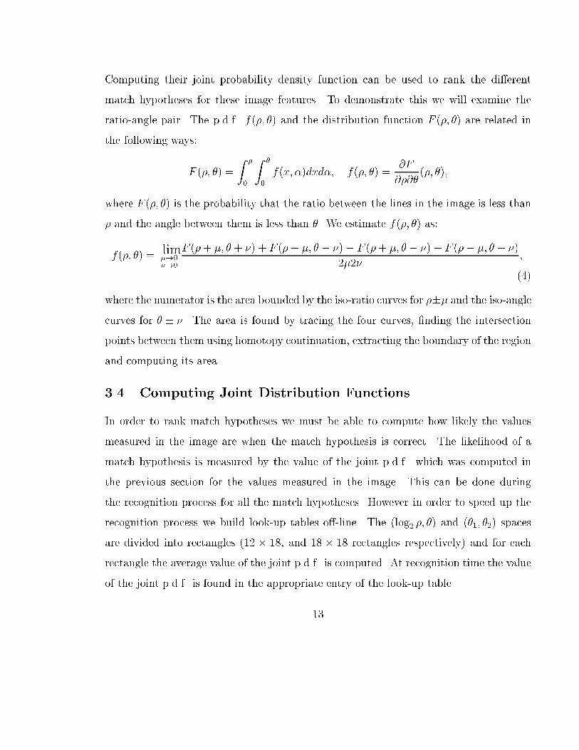
Computing their joint probability density function can be used to rank the di�erentmatch hypotheses for these image features. To demonstrate this we will examine theratio-angle pair. The p.d.f. f(�; �) and the distribution function F (�; �) are related inthe following ways:F (�; �) = Z �0 Z �0 f(x; �)dxd�; f(�; �) = @F@�@� (�; �);where F (�; �) is the probability that the ratio between the lines in the image is less than� and the angle between them is less than �. We estimate f(�; �) as:f(�; �) = lim�!0�!0 F (�+ �; � + �) + F (�� �; � � �)� F (�+ �; � � �)� F (�� �; � + �)2�2� ;(4)where the numerator is the area bounded by the iso-ratio curves for ��� and the iso-anglecurves for � � �. The area is found by tracing the four curves, �nding the intersectionpoints between them using homotopy continuation, extracting the boundary of the regionand computing its area.3.4 Computing Joint Distribution FunctionsIn order to rank match hypotheses we must be able to compute how likely the valuesmeasured in the image are when the match hypothesis is correct. The likelihood of amatch hypothesis is measured by the value of the joint p.d.f. which was computed inthe previous section for the values measured in the image. This can be done duringthe recognition process for all the match hypotheses. However in order to speed up therecognition process we build look-up tables o�-line. The (log2 �; �) and (�1; �2) spacesare divided into rectangles (12 � 18, and 18 � 18 rectangles respectively) and for eachrectangle the average value of the joint p.d.f. is computed. At recognition time the valueof the joint p.d.f. is found in the appropriate entry of the look-up table.13

To perform that we have to compute for two adjacent edges e1 and e2 the probabilityP (�1 < � < �2; �1 < � < �2); (5)that when viewing these edges from a randomly selected viewing direction the ratio ofthe lengths � will be between �1 and �2 and the angle between the edges will be between�1 and �2. We will denote this region of the (�; �) space by R(�1; �2; �1; �2). Using thetechnique described in the previous section we trace the curves of �1; �2; �1 and �2 and�nd the area bounded by them. Because for every value of � or �, there are two curves,two such areas exist. We have divided the (log2 �; �) space into identical rectangles. Thelog2 � dimension was truncated at �k and k where k is an arbitrary limit set takinginto account the maximum and minimum lengths of edges assumed to be extracted bythe edge detector, and using those values to estimate the maximum and minimum ratiosof lengths. Dividing P (�1 < � < �2; �1 < � < �2) by the area of the rectangle inthe (log2 �; �) space yields the average joint p.d.f. value for ratios and angles withinthat rectangle. We have traced the corresponding regions on the viewing sphere of eachrectangle, producing a tessellation of the viewing sphere shown in Fig 5(a). The areas ofthe regions which represent P ((�; �) 2 R(�1; �2; �1; �2)) are plotted in Figure 5(b).For trihedral corner feature sets curves for the two angles are plotted producinga tessellation of the viewing sphere shown in Figure 6(a). The areas of the regionswhich represent P ((�1; �2) 2 R(�11; �12; �21; �22)) were plotted in Figure 6(b). Corners arecharacterized by the three angles between the three pairs of edges. Although the two setsof curves (such as the set in Figure 2(b)) are determined by the �rst two angles, the thirdangle in uences where the two sets of curves will intersect and thus the area of the regions(if they exist). To demonstrate how di�erent the results can be, we have computed thejoint probability function of a number of corners, and display in Figure 7(top) the graphof the probability function. The bottom of the �gure shows the regions which have zero14

(a) (b) -3

-2

-1

0

1

2

0

50

100

150

200

250

300

0

0.02

0.04

0.06

0.08

Θlog

2ρ

Figure 5: The joint probability function of ratios and angles for a pair of edges wherethe original values are (1=3; 90�): (a) tessellation of the viewing sphere into ratio/angleregions; (b) a graph of the joint probability function for ratios and angles as estimatedby the area of the regions in (a).and non-zero probability. This shows that for a given corner there doesn't always exista viewing direction for every pair of angles, where as in the ratio/angle case there existviewing directions for all values of � and �. This enables us to discard some of thehypotheses for trihedral corners because there is no viewing direction which would yieldthose angles for some of the model feature sets.In the ratio/ratio case the feature set includes three edges. We could then measure inthe image in addition to the two ratios, two angles. This means that the ratio/ratio casecan be modeled as an angle/angle and two ratio/angle feature sets. So when a ratio/ratiofeature set occurs in the image it is modeled as a combination of its simpler components.3.5 Dealing with OcclusionUp until now our analysis did not account for the fact that the features we are studyingbelong to solid objects and these objects could partially or totally occlude these features.15

(a) (b) 50

100

150

200

250

300

350

50

100

150

200

250

300

350

0

0.01

0.02

0.03

0.04

0.05

0.06

Θ1

Θ2Figure 6: (a) Tessellation of the viewing sphere into angle/angle regions; (b) a graph ofthe joint probability function for pairs of angles as estimated by the area of the regionsin (a).The features can be occluded by features of the same object or by other objects. Modelingthe e�ects of occlusion between di�erent objects is very di�cult without having priorknowledge about the location of the objects and the camera in the scene.Self occlusion on the other hand can be modeled exactly by dealing with the followingtwo problems: for both types of feature sets the vertex at which the edges meet (thecorner) must be visible, and when computing the ratio of lengths in two edge featuresets, only the length of the visible part of the projection of the edge should be used. Wedetermine the visibility of the features using the aspect graph of the object.As the visibility of features only changes on the viewing sphere on critical curves,we can analyze the visibility of the features in the feature set by studying a representa-tive aspect from each non-critical region, which are bounded by the critical curves, anddetermine where the features are visible and which critical curves bound those regions.Regions in which the corner is not visible are removed from the probability distribution16

50100

150200

250300

350

50100

150200

250300

350

00.020.040.060.080.1

0.120.140.16

50100

150200

250300

350

50100

150200

250300

350

00.010.020.030.040.050.06

50100

150200

250300

350

50100

150200

250300

350

00.010.020.030.040.050.06

50100

150200

250300

350

50100

150200

250300

350

0

0.005

0.01

0.015

0.02

50100

150200

250300

350

50100

150200

250300

350

00.0050.01

0.0150.02

0.0250.03

0.035

Figure 7: For trihedral corners with the following angles: (10�; 20�; 25�), (40�; 60�; 40�),(40�; 60�; 80�), (80�; 80�; 80�) and (90�; 90�; 90�) graphs of joint probability functions andthe regions which have zero and non-zero probability.computed earlier, and for areas in which one or both the edges are partially occludedwe replace the curves traced for the ratio of lengths by new curves using the followingderivation.Given two edges e1 and e2 emanating from a visible vertex p which are shown inFigure 8, we characterize the viewing directions v such that the ratio of the lengths ofthe visible part of their projections is �. So if the projections of e1 and e2 intersect theprojections of e01 and e02 at p+ t1u1 and p+ t2u2 respectively, (1) is modi�ed into:t1ju1 � vj � �t2ju2 � vj = 0: (6)To characterize the intersections of straight lines in a simple way, we use Pl�uckercoordinates, which describe a line by two orthogonal vectors (a;b) where a is somedirection along the line, and if p is a point on the line, b = p� a. We use the followingproperty: two straight lines with Pl�ucker coordinates (a1;b1) and (a2;b2) intersect ifand only if a1 � b2 + a2 � b1 = 0. We write that a line D001 passing through p + tu1 withdirection v intersects the supporting line D01 = (a1; b1) of e01. The line D001 has Pl�ucker17

p

u1

u2

2

1

p+t u1

p+t u22

1

e

e’

e

e2

1

’

Figure 8: Two adjacent edges e1 and e2, starting from a visible vertex p in directions u1and u2 respectively, intersect edges e01 and e02 at p+ t1u1 and p+ t2u2 respectively.coordinates (v; (p+ t1u1)� v). Writing that D01 intersects D001 we obtain:a1 � (t1u1 � v + p� v) + b1 � v = 0:Similarly we obtain for the intersection of e2 and e02:a2 � (t2u2 � v + p� v) + b2 � v = 0:Substituting the equations for t1 and t2 obtained from these equations into (6) yields:�b1 � v � a1 � (p� v)a1 � (u1 � v) ju1 � vj � ��b2 � v � a2 � (p� v)a2 � (u2 � v) ju2 � vj = 0: (7)Squaring this equation yields a degree six homogeneous equation in v. If only one ofthe edges is partially occluded the equation simpli�es to an equation of degree four.To demonstrate the e�ect of occlusion we have chosen two edges of an L shaped objectwhose aspect graph is shown in Figure 9(a). We labeled the non-critical regions of theaspect graph with letters A� F according to the state of occlusion of the two edges andshow representative views of the object in Figure 9(b). In regions labeled by A both18

edges are totally visible therefore (1) is used to trace the iso-ratio curves. In regionslabeled by B the vertex is occluded, and therefore these regions are discarded. In C oneof the edges is partially occluded and in D and E the other edge is partially occluded,each time by a di�erent edge. For these regions (7) is used to trace the iso-ratio curves.In region F the corner is occluded therefore this region is also discarded.In Figure 9(c) the aspect graph and the tessellation of the sphere into regions aretraced on the viewing sphere. It is interesting to note the e�ect of crossing a criticalcurve on the iso-ratio curve. On the boundary between regions A and E the iso-ratiocurve is continuous where as on the boundary between regions A and D or A and C it isnot. In the former when the viewing direction is part of the critical curve the projectionof the occluding edge touches a vertex of one of the edges in the feature set and thereforedoes not occlude it at all. In the latter when the critical curve is passed the edge changesfrom being totally visible to being partially occluded changing the ratio of the visibleparts of the projections of the edges instantaneously. In region F the corner is occludedand on its boundaries e1 (C) and e2 (D and E) become totally occluded yielding setsof dense iso-ratio curves with values converging on zero and in�nity respectively. Theprobability distribution function is shown in Figure 9(d) (compare to Figure 5 whichdisregards occlusion). Similar probability distributions have been computed for the caseof the trihedral corner. In that case regions on the viewing sphere where the corner is notvisible were discarded. In the other regions the regular iso-angle equations were used.4 Ranking Match HypothesesIn this section we use the techniques presented in the previous section for ranking matchhypotheses. We build look-up tables of lists of hypotheses sorted by probability o�-lineand during the recognition stage the sorted hypotheses are tested. We will assume for19

(a) BB

B

A

A

A

A

C F

ED

(b)(A) (B) (C)(D) (E) (F )

(c) (d)-3

-2

-1

0

1

2

0

50

100

150

200

250

300

0

0.005

0.01

0.015

0.02

0.025

Θlog

2ρ

Figure 9: (a) the aspect graph of the L shaped object with the regions marked by lettersA-F; (b) views of the object: (A) both edges are visible; (B) at least one of the edges isnot visible; (C) one of the edges is partially occluded; (D)-(E) the other edge is partiallyoccluded by two di�erent edges; (F) the corner is occluded; (c) tessellation of the viewingsphere into regions; (d) a graph of the joint probability function as estimated by the areaof the regions in (c). 20

now that all feature sets detected in image are due to objects in the model database. Weshall relax that assumption in the next section.4.1 Building Look-up TablesIn the preprocessing stage, we construct two look-up tables T1(�; �) and T2(�1; �2) for theratio/angle and angle/angle pairs respectively. The tables are built by computing jointprobability distributions which were described in Section 3.4 for all feature sets of allmodels in the model database.We use these probabilities to determine the induced probabilities on the identity ofthe object. We denote by E a feature set measured in the image with values within acertain region of the (�; �) or (�1; �2) space, by Mi the event in which the ith model fromthe database appears in the image, and by H(i)j the hypothesis that the jth model featureset of the ith model matches E. We would like to compute P (H(i)j ;MijE) which is theprobability that hypothesis H(i)j is correct if E was measured in the image. Using Bayes'law P (H(i)j ;MijE) = P (E;H(i)j jMi)P (Mi)P (E) :P (E;H(i)j ; jMi) is the probability that features associated with hypothesis H(i)j werevisible and that the values measured in the image were within the region of E assumingthat object Mi is visible in the scene. This probability was computed in the previoussection. P (E) is the sum of all the probabilities of all the hypotheses in which E can bemeasured. Therefore, P (E) =Xm Xj P (E;H(m)j jMm)P (Mm):21

Combining these two equations yields:P (H(i)j ;MijE) = P (E;H(i)j jMi)P (Mi)PmPj P (E;H(m)j jMm)P (Mm) : (8)P (Mi) can be determined using any prior knowledge we have about the likelihood ofa model to appear in the image. We keep in tables an entry for each E. In each entrythere is a list of hypotheses due to E. P (H(i)j ;MijE) is computed for the hypothesesin the list. This is repeated for all the entries in the tables and the lists are sorted byprobability.It is important to note that the regions in the (�; �) or (�1; �2) spaces do not haveto be of equal size. Moreover, the recognition algorithm will perform better if regionswith multiple probabilistic peaks are divided into smaller regions with one peak in each.Thus each hypothesis would have a higher probability in the subregion in which its peakis located and a lower probability in the other subregion, where as if only one regionexisted all the hypotheses would have the same average probability. In general, the (�; �)or (�1; �2) space can be partitioned using a quad-tree approach where a region is dividedinto four regions only if the order of the hypotheses of the subregions is di�erent thanthe order of the hypotheses of the parent region.4.2 Dealing With UncertaintyThe input to the recognition phase of the algorithm is the result of edge and cornerdetection performed on the image. There is uncertainty in this data which has to bemodeled in order to design a robust algorithm. We identify three types of uncertaintywhich have to be dealt with: certain feature sets which appear in the image will notbe recovered by the edge and corner detectors, the image features might not match anymodel features, and the values measured for image features are themselves uncertain.22

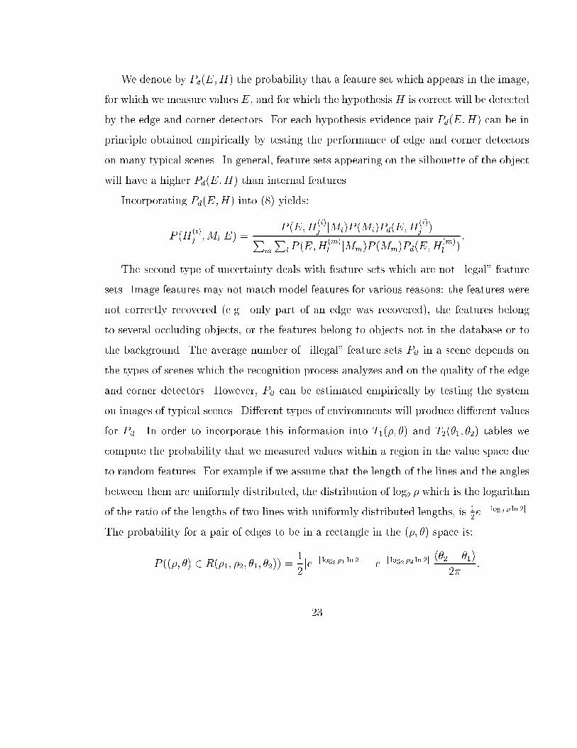
We denote by Pd(E;H) the probability that a feature set which appears in the image,for which we measure values E, and for which the hypothesis H is correct will be detectedby the edge and corner detectors. For each hypothesis evidence pair Pd(E;H) can be inprinciple obtained empirically by testing the performance of edge and corner detectorson many typical scenes. In general, feature sets appearing on the silhouette of the objectwill have a higher Pd(E;H) than internal features.Incorporating Pd(E;H) into (8) yields:P (H(i)j ;MijE) = P (E;H(i)j jMi)P (Mi)Pd(E;H(i)j )PmPl P (E;H(m)l jMm)P (Mm)Pd(E;H(m)l ) :The second type of uncertainty deals with feature sets which are not \legal" featuresets. Image features may not match model features for various reasons: the features werenot correctly recovered (e.g. only part of an edge was recovered), the features belongto several occluding objects, or the features belong to objects not in the database or tothe background. The average number of \illegal" feature sets Pil in a scene depends onthe types of scenes which the recognition process analyzes and on the quality of the edgeand corner detectors. However, Pil can be estimated empirically by testing the systemon images of typical scenes. Di�erent types of environments will produce di�erent valuesfor Pil. In order to incorporate this information into T1(�; �) and T2(�1; �2) tables wecompute the probability that we measured values within a region in the value space dueto random features. For example if we assume that the length of the lines and the anglesbetween them are uniformly distributed, the distribution of log2 � which is the logarithmof the ratio of the lengths of two lines with uniformly distributed lengths, is 12e�j log2 � ln 2j.The probability for a pair of edges to be in a rectangle in the (�; �) space is:P ((�; �) 2 R(�1; �2; �1; �2)) = 12 je�j log2 �1 ln 2j � e�j log2 �2 ln 2jj(�2 � �1)2� :23

The probability for a corner to be in a rectangle in the (�1; �2) space is:P ((�1; �2) 2 R(�11; �12; �21; �22)) = (�12 � �11)2� (�22 � �21)2� :In each entry in the tables a new hypothesis is added to the list, which represents the\illegal" feature set and whose probability is the probability calculated above multipliedby Pil.The last type of uncertainty is in the values measured in the image. For the two-edge case we assume that there is uncertainty in vertex position of the three vertices.We assume the six coordinates a = (x1; y1; x2; y2; x3; y3) have a normal distribution withmean �i = ai and variance �2 which can be determined empirically. This induces aprobability distribution on � and � which enables us to compute the probability that theactual measured values are in a region of the (�; �) space. ThusP (HjE) =Xk P (HjEk)P (EkjE) =Xk P (HjEk) P (EjEk)P (Ek)Pj P (EjEj)P (Ej) ;where P (EjEk) is the probability that E is in the kth region of the (�; �) space. P (EjEk)decreases rapidly as the distance from E to the region Ek increases, and the rate ofthe decrease accelerates as �2 gets smaller. Therefore for most regions Ek except theones close to E, P (EjEk) is negligible and P (HjE) is computed by summing over thecontributions of a small number of regions.5 Pose and Pose Uncertainty EstimationFor all correct hypotheses which match features from an instance of an object to featuresin the model, the pose recovered for all of these match hypotheses should be the same.Therefore we use pose estimation to �nd sets of hypotheses which produce the samepose to reinforce the recognition hypothesis. Uncertainty in the values measured in the24

image induces uncertainty in the pose and has to be accounted for when testing thecompatibility of match hypotheses.5.1 Pose EstimationThe problem of estimating the pose from three points [1, 19, 21] or a trihedral corner [32]has been extensively studied. We present here a simple approach which deals with bothtypes of feature sets. We regard the pose of an object in weak perspective projection asa combination of the following four components:� a viewing direction v which is a point on the viewing sphere,� a rotation of the image by � degrees about the viewing direction,� a scale s,� a translation t in the image.Therefore the pose is a point in the six dimensional space fS2�[0 � � � 2�]�[smin � � � smax]�IR2g where S2 is the unit viewing sphere, smin and smax are the minimum and maximumassumed scales respectively, and the translation t must be a vector in the image. Theprojection pi of a point p of the object in the image is:pi = sR(�)(p � v2; p � v3) + t; (9)where v;v2;v3 is an orthonormal basis of IR3 and R(�) is a rotation by � degrees.We will now show what components of the pose can be recovered from angles andlengths measured in the image given an hypothesis which matches a minimal number offeatures in the image to features in the model. Each measured angle or ratio imposes aone-dimensional constraint on possible viewing directions. In order to determine v twosuch constraints are needed. Two pairs of types of curves were considered: the ratio/angle25

pair and the angle/angle pair. The ratio/ratio pair is not considered because in orderto measure two ratios we would need an hypothesis which contains additional matchedfeatures which we are trying to avoid. v is obtained as the intersection points betweentwo curves. The degrees of the ratio and angle curves are 2 and 4 respectively. Thereforethe number of intersection points found for the ratio/angle and angle/angle pairs willbe at most 8 and 16 respectively. However as shown in Section 3 the angle equationsgenerate curves for �; � � �; 2� � � and �(� � �). As most of the solutions are for theother angles the number of real solutions is much less. Some of the remaining solutionscan be eliminated by visibility considerations (i.e., the features are occluded from thatviewing direction). The other components of the pose are determined using standard 2Dpose estimation. The rotation angle � is determined for both pairs by rotating the resultsof applying the projection of the object in direction v until the corresponding edges areparallel to each other. The scale and translation can not be obtained for the angle/anglecase. Therefore only in the case of the ratio/angle pair they are recovered.5.2 E�cient Pose Uncertainty EstimationWe compute the pose p of the object assuming a match hypothesis h is computed usingthe technique described in Section 5.1. p is a function of the vertex positions a measuredin the image. Using Taylor expansion, the e�ect of a small uncertainty � in a on the posecan be estimated by: p(a+ �) � p(a) +rp(a)�:As the uncertainty is small, the contributions of higher derivatives of the pose functioncan be neglected. For the ratio/angle case all six components of the pose are recoveredusing three coordinate pairs. Thusrp(a) is a 6�6 matrix. Assuming that the uncertaintyfor each coordinate pair is bounded by �, the maximum uncertainty for a component p�26

of pose will be when � has the following values:(�2i�1= � @p�@a2i�1 ( @p�@a2i�1 2 + @p�@a2i 2)�1=2;�2i = � @p�@a2i ( @p�@a2i�1 2 + @p�@a2i 2)�1=2;where i denotes the ith coordinate pair. Thus for each coordinate pair the vector(�2i�1; �2i) points in the direction of rp�(a2i�1; a2i). The derivatives are computed nu-merically. The perturbed pose is computed using the multivariate Newton-Raphsonalgorithm with the unperturbed pose given as the initial guess. For most components ofthe pose computing the uncertainty is simple. However for the viewing direction com-ponent v of the pose we parameterize the pose as v = �v1 + �v2 + v3 where v1 is theviewing direction for the unperturbed input, � =p(1� �2 � 2), and the uncertainty ismeasured in radians in the v2 and v3 directions. So if the viewing direction uncertaintiesare arcsin� and arcsin , the viewing direction component in the pose uncertainty regionis: fv 2 S2 : jv � v2j < �; jv � v3j < g:In order to check if two pose uncertainty regions have a non-empty intersection, theregions of all components of the pose (viewing sphere,rotation,scale,translation) have tointersect. This works for pairs of ratio/angle hypotheses, but for angle/angle hypothesesonly the viewing direction and rotation components can be recovered directly and moreinformation is needed to recover the scale and translation components. By adding tothe feature set the position and uncertainty of the corner of the other feature set, thescale and translation components of the uncertainty region are also recovered Then theintersection of all the components is tested.To demonstrate the variability of the pose uncertainty for di�erent model feature sets,we tabulate the pose uncertainty for them in Table 1 where the ratio and the angle in theimage were 1.4 and 315� respectively. The sizes of nearly all the components of the pose27

region do not change much between the di�erent examples. Only the size of the viewingsphere component changes dramatically for the di�erent examples. The closer the ratioand angle measured in the model are to the values measured in the image the larger theviewing sphere component is. This phenomenon, is another aspect of the probabilisticpeaking e�ect. Thus, hypotheses with low probability (viewed values very di�erent fromreal values) will have smaller pose uncertainty regions which will reduce the chance thatthere will be an intersection between the pose uncertainty regions of two such hypotheses,reducing the chance for false a positive recognition result.Ratio Angle Viewing Sphere Rotation Scale Translation1.0 280:0� 0.011 0.092 0.139 0.00800.3 90:0� 0.001 0.101 0.147 0.03291.4 315:0� 0.085 0.184 0.158 0.04590.3 315:0� 0.001 0.109 0.173 0.00991.4 90:0� 0.009 0.124 0.114 0.0142Table 1: Tabulation of the size of components of the pose uncertainty region for a givenimage feature set whose ratio and angle are 1.4 and 315:0� respectively for several modelfeature sets with di�erent ratios and angles. Note that for measured values equal to thereal values the uncertainty region is much larger (up to a factor of 85 in this example).6 Ranking Recognition Results6.1 RequirementsIn the �nal stage of the algorithm, pairs of hypotheses whose pose uncertainty regionshave a non-empty intersection are ranked by probability. For a ranking scheme to beuseful it should exhibit the following characteristics:� Using the notion of \maximum likelihood interpretations" discussed in [30], morelikely interpretations (hypotheses with larger pose uncertainty regions) should beranked higher than less likely ones. 28

� Interpretations which would assume a larger uncertainty in vertex position shouldbe ranked lower than interpretations with smaller uncertainty.� Feature combinations with many plausible interpretations (e.g., features belongingto a single rectangular or triangular face) should be ranked lower than featurecombinations with a unique interpretation.Our probabilistic expression accounts for all these sometime con icting requirements inranking possible interpretations. In addition, the algorithm should be able to rank thecorrect hypotheses �rst even if the algorithm has to be stopped for lack of time beforeall pairs of hypotheses have been tested.6.2 DerivationGiven a set of image features which participate in a match hypothesis (ratio/angle orangle/angle), the pose uncertainty region bounds the region in the pose space in whichthe error is bounded by �. The higher the value of � the higher the probability that ifthe hypothesis is correct, that the pose of the object lies within the uncertainty region.� is set large enough such that the probability that the correct pose is not within theuncertainty region is very small.Given two feature sets in the image e1 and e2 and two respective hypotheses h1 andh2, we de�ne H as the hypothesis that h1 and h2 are true and both match image featuresets to the same instance of a certain modelM . We compute P (h1; h2; H;M je1; e2), usingBayes' rule: P (h1; h2; H;M je1; e2) = P (e1; e2; h1; h2; H;M)P (e1; e2) : (10)For e1 and e2 to be features of the same object, the pose of the object p must be inthe intersection of the pose uncertainty regions of the two hypotheses which we denote29

by U(e1; h1) and U(e2; h2) respectively. For each possible pose we writeP (e1; e2; h1; h2; H;M; p) = P (M)Pd(e1; h1)Pd(e2; h2)�U(e1;h1)(p)�U(e2;h2)(p)fp(p);where �U(e1;h1)(p) and �U(e2;h2)(p) are the characteristic functions of U(e1; h1) and U(e2; h2)respectively and fp(p) is the p.d.f. of poses in the pose space. If the position of the cam-era with respect to the surface on which the objects are placed is known, informationabout stable poses of the objects can be re ected in fp(p). By marginalizing with respectto p we obtainP (e1; e2; h1; h2; H;M) = P (M)Pd(e1; h1)Pd(e2; h2) Zp �U(e1;h1)(p)�U(e2;h2)(p)fp(p)dp:(11)When there is no information about the pose of the camera we have to assume thatposes are uniformly distributed and that the volume of the pose space is normalized to1. In this case (11) simpli�es to:P (e1; e2; h1; h2; H;M) = P (M)Pd(e1; h1)Pd(e2; h2)jU(e1; h1) \ U(e2; h2)j: (12)We compute P (e1; e2) by summing over every pair of hypotheses hi; hj which couldgenerate e1 and e2 respectively and whether e1 and e2 belong to the same object (H(i;j))or not (:H(i;j)), yielding:P (e1; e2) =PiPj P (e1; e2; hi;M (hi); hj;M (hj ); H(i;j)) +PiPj P (e1; e2; hi;M (hi); hj;M (hj);:H(i;j));where M (hi) is the model to which the model features of hi belong. In the �rst term e1and e2 are feature sets of the same instance of a certain model, so the probabilities arecomputed in the same way that as the numerator of (10). In the second term, e1 and e2do not belong to the same object, thereforeP (e1; e2; hi;M (hi); hj;M (hj);:H(i;j)) = P (e1; hi;M (hi))P (e2; hj;M (hj))P (:H(i;j)):30

P (:H(i;j)) is computed empirically from typical scenes as the probability that M (hi)and M (hj ) will both appear in an image. We use the same arguments that were used toderive (11) to compute P (e1; hi;M (hi)), by taking the volume of one uncertainty regioninstead of the intersection of two regions, yielding:P (e1; hi;M (hi)) = P (M (hi))Pd(e1; hi)jU(e1; hi)j: (13)Combining all these results we are able to compute P (h1; h2; H;M je1; e2).This derivation can be easily extended to more than two hypotheses. In the numeratorof (10) we compute the intersection of the uncertainty regions of all the hypotheses andin the denominator we sum over all possible interpretations of the feature sets underconsideration (all the features belong to the same object, some of them belong to oneothers to another etc...). We use the results for all subsets of the set of features in orderto compute that expression. It is important to note that only sets of features that allof their subsets have non-zero rank might have a non-zero rank themselves. Therefore,we only consider the small number of pairs of hypotheses which have been found by thepair-ranking procedure as input for the extended procedure, which can be performed atminimal computational cost but have very statistically signi�cant results.During recognition, for every pair of hypotheses whose pose uncertainty regions in-tersect we evaluate (10). Terms similar to P (e1; e2; hi; hj;M;H(i;j)) appear in the nu-merator and the denominator of the expression. For hypothesis pairs whose pose un-certainty region do not intersect, this term will be zero. Therefore, when we computethe rank of a hypothesis pair we can assume at �rst that all the terms of that typeexcept P (e1; e2; h1; h2; H) are zero. When we compute the rank of another hypothesispair h01 and h02 which interpret the same image feature sets, we will add the value wecomputed for P (e1; e2; h01; h02;M 0; H) to the denominator of the rank of h1 and h2. Termsof the type P (e1; hi;M (hi)) which also appear in the denominator only involve one hy-31

pothesis, therefore their value can be pre-computed and stored in the look-up tables.However that is not always necessary because as the following calculation will show,their values may be very small and their impact on the value of (10) is negligible. Wedetermine whether to neglect these terms by analyzing the relative sizes of terms of thetype P (e1; e2; hi; hj;M;H(i;j)) and Pi;j P (e1; e2; hi;M (hi); hj;M (hj);:H(i;j)) and when theformer is much bigger than the latter, the latter can be discarded.We estimate jU(e1; h1) \ U(e2; h2)j, in order to estimate the value ofP (e1; e2; hi; hj;M;H(i;j)). Consider the case of the one dimensional pose space and thatU(e1; h1) and U(e2; h2) are segments of length l which overlap. When the relative po-sitions of U(e1; h1) and U(e2; h2) are uniformly distributed, the average length of theoverlap between them will be l=2. Generalizing this to the six-dimensional pose space,we estimate that jU(e1; h1) \ U(e2; h2)j � jU j=26, where jU j is the average volume of apose uncertainty region. Consider the recognition system with a database of m models.Each model has on average n feature sets, and on average k of them appear in a givenscene. We can estimate P (M) � k=m. Thus we can estimate thatP (e1; e2; hi; hj;M;H(i;j)) � 2�6jU j(k=m)Pd(e; h)2;andXi;j P (e1; e2; hi;M (hi); hj;M (hj);:H(i;j)) � ( km)2(nm)2jU j2Pd(e; h)2 = k2n2jU j2Pd(e; h)2The ratio between these two values yields:P (e1; e2; hi; hj;M;H(i;j))Pi;j P (e1; e2; hi;M (hi); hj;M (hj);:H(i;j)) � 2�6jU j(k=m)Pd(e; h)2k2n2jU j2Pd(e; h)2 � 126kn2mjU j : (14)Evaluating (14) for a recognition system such that k � 1,n � 10 and jU j � 10�7, gives1500=m. Only when the number of models in the database m > 100 will the contribution32

of Pi;j P (e1; e2; hi;M (hi); hj;M (hj);:H(i;j)) to (10) be signi�cant, for a smaller databasethis term can be neglected.The recognition algorithm traverses the list of the pairs of hypotheses in decreasingprobability order. We compute the rank of pairs of hypotheses whose pose uncertaintyregions have a non-empty intersection by �rst evaluating (12) and dividing it by the sumof all the values of (12) computed for all the pairs of hypotheses found so far whichsuggest interpretations to the same pair of features.6.3 Characteristics of the Ranking SchemeIn section 6.1, we made several requirements of our ranking scheme. Here we will analyzethe algorithm to see how it satis�es these requirements.We have required that \popular" features which yield many possible interpretations(e.g., features which belong to a rectangular or triangular face) be ranked lower thanfeatures which yield few interpretations. \Popular" features will participate in manyhypothesis sets. Therefore their corresponding value of P (e1; e2; h1; h2; H;M) will con-tribute to the denominators of the probabilities of all the interpretations, thus reducingthe ranks of them all. This is reasonable because this set of features does not allow us todiscriminate between the di�erent hypotheses, where as a less \popular" but probablycorrect set of features will have a higher rank, since not many competing hypotheses willexist for that set of features.We have required that even if the algorithm had to be stopped without checking allpairs of hypotheses, the correct recognition results would be ranked high on the list. Asthe hypotheses are traversed in decreasing probability order there is a high probabil-ity that the correct hypothesis pairs will be ordered high on the list. Therefore, if therecognition process has to be interrupted, we can still assume that the match hypothe-ses corresponding to the correct interpretation have been processed. We are especially33

interested in the \non-popular" feature sets. For them the correct interpretation hasbeen found and there is a small chance that any other competing interpretations wouldhave been found even if all pairs of hypotheses had been checked. Therefore most \non-popular" hypotheses will have a high rank and that rank would be equal to the �nal rankin many cases.We also made several requirements on how competing interpretations for the same setof features should be ranked. We demonstrate the performance of the ranking algorithmusing illustrations of pose uncertainty regions of typical hypothesis pairs showed in Figure10.(a) (b)Figure 10: Illustration of the performance of the ranking scheme. Each uncertainty regionof an hypothesis is illustrated by a rectangle, their intersection is illustrated by a shadedrectangle. (a) the algorithm ranks higher a pair of likely hypotheses with large poseuncertainty regions (left) than a pair of unlikely hypotheses with small pose uncertaintyregions (right); (b) the algorithm ranks higher a hypothesis pair with a small error invertex position (left) over a pair with a large error (middle) but can not prefer the pairon the right to the pair on the left even though the error for that pair is larger.The algorithm ranks competing interpretations for a pair of features by comparingthe intersection of the pose uncertainty regions of the two pairs of hypotheses. In Figure10(a), a pair of likely hypotheses with large pose uncertainty regions (left) are rankedhigher than a pair of unlikely hypotheses with small pose uncertainty regions(right).Thus the algorithm would prefer the \maximum likelihood" interpretation [30] over theless likely interpretation. In Figure 10(b), we study the case in which the size of the34

pose uncertainty regions is the same but their relative positions are di�erent. The closerthe centers of the regions are, the smaller the error in vertex position will be if theinterpretation is correct. The algorithm ranks higher the hypotheses pair with a smallerror in vertex position(left) over a pair with a large error(middle) which causes theiruncertainty regions to not fully intersect. The algorithm however does not rank the pairon the left higher than the pair on the right even though the pair on the right assumesa larger uncertainty in vertex position because the size of the intersection of the poseuncertainty regions is the same. In the next section we present a variant of the rankingscheme which addresses this problem.6.4 Exact Ranking SchemeThe fundamental characteristic of the algorithm which prevents it from discriminatingbetween the two interpretations illustrated in Figure 10(b)(left,right) is that all poseswithin the intersection of the pose uncertainty regions have equal weight even thoughthe poses which yield small vertex position errors should have a higher weight than poseswhich yield large errors.To solve this problem we will weight each pose by the distance between the image fea-tures and the model features back-projected using that pose. Assuming the uncertaintyin vertex position has a normal (or any other known) distribution, we use the probabilitydensity function value for the computed vertex position uncertainty as the weight forthat pose. Substituting this expression into (11) yields:P (e1; e2; h1; h2; H;M) = P (M)Pd(e1; h1)Pd(e2; h2) Zp f1(p)f2(p)fp(p)dp; (15)where f1(p) and f2(p) denote the probability density functions applied to the errors ine1 and e2 respectively assuming the pose is p.35

Similarly (13) is transformed into:P (e1; hi;M (hi)) = P (M (hi))Pd(e1; hi) Zp f1(p)fp(p)dp:This ranking scheme correctly ranks 10(b)(left) higher than 10(b)(right). In order touse this scheme we would have to evaluate expressions of the type (15) during recognitiontime. There is no closed form solution for evaluating integrals of that type and numericalMonte-Carlo integration techniques must be used. These techniques are computationallyvery costly so we recommend using the simpler recognition ranking scheme presented inSection 6.2.7 Experimental Recognition ResultsIn this section we present the implementation of our recognition algorithm and showexperimental results of running it on real images. Our model database consists of theseven objects shown in Figure 11.We extract edges from the image using the Canny edge detector [10] and then detectlines from the extracted edges. We combine these lines automatically into feature setsusing the following technique: we detect corners in the image as the intersection point ofthe supporting lines of two lines in the image when the actual termination points of thetwo lines is close to the intersection point. Once a corner has been detected, additionallines which terminate close to the corner are added to the list of lines emanating from it.We label lines which end in the middle of another line (T junctions) as partially occludededges. We generate feature sets from this information. For each line triple emanatingfrom a corner, we generate an angle/angle feature set. For each pair of lines emanatingfrom a corner, we generate an ratio/angle feature set when both lines start and end ata vertex, or an occluded ratio/angle feature set when one or both of them ends at a T36

(a) (b) (c) (d)(e) (f) (g)Figure 11: Model database: (a) a truncated pyramid, (b) a box, (c) a triangular prism,(d) another prism, (e) a pyramid, (f) a tape dispenser, (g) an L shaped object.junction. The feature sets extracted in this stage need not be perfect and not all visiblefeatures sets must be found because an important feature of our recognition algorithm isthat it is robust to uncertain and incomplete input.For each feature set, we retrieve from the look-up tables the corresponding matchhypotheses and their probabilities. Occlusion is accounted for in matching the featuresets with the match hypotheses. A list of pairs of hypotheses is generated. The a-prioriprobability estimate for each such pair is set as the product of probabilities of the twohypotheses which has been retrieved from the look-up table. This list is then sorted byprobability and processed in that order. For each hypothesis pair, we test if their poseuncertainty regions intersect. We compute the rank of each compatible pair of matchesfound and maintain a list of compatible pairs of matches sorted by rank. The algorithmoutputs the interpretations due to the pairs of matches with the highest ranks. As was37

explained in Section 6.2, this ranking scheme can be extended to deal will larger sets offeatures with a small extra computational cost. In this implementation however, onlypairs of matches were considered.To make this algorithm a complete recognition system the following two steps haveto be added: least squares estimation of pose, and hypothesis veri�cation by back-projection. These two steps have not been implemented since the focus was put on�nding e�cient ways to generate promising hypotheses.We now present several examples of results obtained running our algorithm on realimages. Figure 12(a) shows an image of the rectangular pyramid and the second prism.Note that the results of the edge detection and line extraction (Figure 12(b)) containfeatures that are due to the background and shadows. Figure 12(c) shows the featuresbelonging to feature sets extracted from the image. Note that the line due to the shadowof the prism is part of angle/angle feature sets where the other lines participating in thosefeature sets are edges of the prism itself. Edges which have not been fully extracted bythe edge detector may only participate in angle/angle feature sets and are discardedwhen they are not adjacent to a trihedral corner. Applying this criterion to this imagecaused most features due to the background to be discarded. The objects recognized bythe algorithm are shown in Figure 12(d).Results of running the algorithm on an image of two triangular prisms with partialocclusion are shown in Figure 13. Note that the edge detector was not able to recoverthe internal edge of the triangular shape but found all the silhouette edges.In Figure 14, the results of processing another image of the two triangular prismswith partial occlusion are shown. Here, a di�erent part of the second prism is occluded.Note that again internal edges were not detected by the edge detector. The internal edgeof the second prism is especially interesting. Parts of the edge were detected but not thewhole edge. Therefore the segments of the edge participate only in angle/angle feature38

(a) (b) (c) (d)Figure 12: Recognition results for an image of a rectangular pyramid and a prism: (a)the image; (b) the results of edge and line detection; (c) feature sets recovered from theimage; (d) recognized objects.(a) (b) (c) (d)Figure 13: Recognition results for an image of two triangular prisms with partial occlu-sion: (a) the image; (b) the results of edge and line detection; (c) feature sets recoveredfrom the image; (d) recognized objects.sets but not in ratio/angle feature sets.In Figure 15, the results of processing an image of the tape dispenser are shown.Note that the the object is not purely polyhedral but even so the program was able torecognize the object. As usual only some of the visible features were detected by theedge/line detector. One of the ratio/angle feature sets is partially occluded. Naturallyit was matched only to model feature sets where the corresponding edge was partiallyoccluded. As these hypotheses are quite rare in our database, the correct hypothesis gota very high score and participated in the �rst hypothesis pair that was found and the39

(a) (b) (c) (d)Figure 14: Recognition results for another image of two triangular prisms with partialocclusion: (a) the image; (b) the results of edge and line detection; (c) feature setsrecovered from the image; (d) recognized objects.hypothesis pair was correct.(a) (b) (c) (d)Figure 15: Recognition results for an image of the tape dispenser: (a) the image; (b)the results of edge and line detection; (c) feature sets recovered from the image; (d)recognized object.We collected in Table 2 statistics regarding the run of the algorithm on the examplesshown above. For each run, we tabulated the number of feature sets extracted from theimage, the number of match hypotheses retrieved from the look-up tables, the number ofpairs of match hypotheses which were tested for compatibility, the number of compatiblepairs found, how many of them were correct and how many of the �rst ten compatiblepairs ranked by probability were actually correct and their ranks.In Table 3, we display the running times of the algorithm on the four images. Foreach run we tabulated the time it took until all the hypothesis pairs were generated and40

sorted, the time it took the algorithm until a correct hypothesis pair of one of the twoobjects has been tested and found to be correct, the time until a correct hypothesis pairbelonging to the other object is tested and the total run time of the algorithm whichterminates after testing all hypothesis pairs. The algorithm was implemented in C++and run on a Sun E450 server.It is important to note that due to the rank of the match hypotheses most of thecorrect results will be found early in the run of the algorithm and there is no needto test all possible hypothesis pairs. Also note that our main concern was to explorethe concepts underlying these algorithms, and little e�ort was made to implement thisalgorithm e�ciently.Figure Feature Match Hypothesis Possible Correct Correct ResultsSets Hypotheses Pairs Results Results of the 10 HighestRanked Results12 25 4865 667904 877 192 3 (5,9,10)13 11 2221 100076 318 25 2 (8,9)14 16 3117 206575 627 58 4 (3,4,6,8)15 11 2278 110265 135 23 7 (1-3,4-7,9)Table 2: The recognition results table shows statistics from various stages of the run ofthe recognition algorithm.Figure Time Until Hypothesis Time Until First Time Until Second TotalPairs are Generated Object Hypothesis Object Hypothesis Run Time12 15 sec 17 sec 57 sec 177 sec13 2 sec 4 sec 11 sec 22 sec14 5 sec 6 sec 10 sec 86 sec15 3 sec 3 sec N/A 11 secTable 3: Timing of the run of the algorithm: time until the hypothesis pairs are generated;time until the �rst hypothesis pair which correctly recognizes the �rst object was tested;time until the �rst hypothesis pair which correctly recognizes the second object wastested; time until the algorithm completed.41

We show several incorrect hypothesis pairs found by our algorithm in Figure 16 inorder to characterize them and suggest methods to avoid processing the pairs of matcheswhich yielded them in the �rst place. In Figure 16(a), the interpretation of the sceneis correct, only the pose of the object is wrong. However, as the internal edges of theobject were not found by the edge detector there is no way to distinguish between thecorrect and incorrect pose, they both yield the same silhouette. A similar example isshown in Figure 16(b). However in this case internal edges were recovered by the edgedetector and the correct match should be ranked higher when more features are addedto the match.The examples in Figures 16(c,d) show how any rectangular or triangular face can bematched to any other face of the same type. In order to avoid this type of erroneous pairsof matches, it is better not to process pairs of hypotheses whose model features belongto the same face at all. Although correct hypothesis pairs will also be discarded, theperformance of the recognition algorithm will not be hurt because the algorithm couldnot distinguish between the correct pair and the many incorrect ones and gives them alla low rank.(a) (b) (c) (d)Figure 16: Wrong recognition results: (a) the triangular object with an incorrect pose;(b) the triangular object with another incorrect pose which contradicts some of the otherfeatures extracted from the image; (c) a triangular face of the triangular object is matchedto a face of the truncated pyramid; (d) a rectangular face of the prism is matched to thewrong rectangular face of the prism. 42

We therefore re-ran the algorithm discarding all pairs of hypotheses which lie on thesame face and all hypotheses which have edges in common. The results are presentedin Tables 4 and 5. The number of hypothesis pairs has been reduced somewhat, andthe running time has also improved. The major di�erence is the reduction by a factor of10-80 of the number of recognition results found. Most of the remaining results left arecorrect. As a result there are more correct results in the top 10 results. Therefore, notonly will the total number of results which might have to be veri�ed is reduced, a correctanswer will be one of the �rst tested.In order to test the e�ects of clutter on our algorithm, we re-ran the program on Figure15 to which we added 10 and even 30 random feature sets. In both cases the programran longer but not even one additional false result was found. This demonstrates thefact that problem of incorrect results is usually not due to clutter but is due to similaritybetween models.Figure Feature Match Hypothesis Possible Correct Correct ResultsSets Hypotheses Pairs Results Results of the 10 HighestRanked Results12 25 4865 620181 69 54 6 (4-5,6-10)13 11 2221 92966 4 4 4 (1-4)14 16 3117 189204 24 12 5 (2,5,8-10)15 11 2278 101842 10 9 9 (1-8,10)Table 4: The recognition results table shows statistics from various stages of the secondrun of the recognition algorithm.8 DiscussionIn this paper we have presented a probabilistic 3D object recognition algorithm. We havestudied the nature of the iso-ratio and iso-angle curves and traced them on the viewingsphere. We have used these curves to accurately compute conditional probabilities that43

Figure Time Until Hypothesis Time Until First Time Until Second TotalPairs are Generated Object Hypothesis Object Hypothesis Run Time12 18 sec 22 sec 41 sec 134 sec13 3 sec 10 sec 11 sec 21 sec14 6 sec 10 sec 28 sec 63 sec15 3 sec 3 sec N/A 10 secTable 5: Timing of the run of the algorithm with \popular" feature set pairs removed:time until the hypothesis pairs are generated; time until the �rst hypothesis pair whichcorrectly recognizes the �rst object was tested; time until the �rst hypothesis pair whichcorrectly recognizes the second object was tested; time until the algorithm completed.image features match model features. The probabilities have been incorporated into aprobabilistic model which takes into account the uncertainties inherent in the input tothe recognition algorithm. These probabilities have been used to decide the order inwhich to process the match hypotheses. We have developed a method to compute thepose of the object using a minimal feature set in the image which matches to featureset in the model database. Taking the uncertainty in values measured in the image intoaccount, we have computed the uncertainty pose region for each hypothesis. By �ndinghypotheses whose pose regions have a non-empty intersection, we have been able to �nda set of feature sets which reinforce the recognition hypothesis. We have ranked thesehypotheses by computing the probability that all the feature sets in the set came fromthe same instance of the suggested object.Future work will be dedicated to improving the e�ciency of the algorithm by �ndingbetter ways to order the rank hypotheses, process hypothesis pairs and �nd smaller andmore accurate pose uncertainty regions. Another important research direction would beto extend this probabilistic recognition scheme to deal with more complicated objectssuch as curved objects.44

AcknowledgmentsThis work was supported in part by the Beckman Institute and the Center for AdvancedStudy of the University of Illinois at Urbana-Champaign, by the National Science Founda-tion under grant IRI-9224815, and by the National Aeronautics and Space Administrationunder grant NAG 1-613.References[1] T. D. Alter. 3D pose from 3 points using weak-perspective. IEEE Trans. Patt. Anal. Mach. Intell., 16(8):802{808,August 1994.[2] T. D. Alter and D. W. Jacobs. Error propagation in full 3D-from-2D object recognition. In Proc. IEEE Conf. Comp.Vision Patt. Recog., pages 892{898, Seattle, Washington, June 1994.[3] R. D. Arnold and T. O. Binford. Geometric constraints in stereo vision. In Proc. SPIE meeting, San Diego, California,July 1980.[4] N. Ayache and O. D. Faugeras. HYPER: a new approach for the recognition and positioning of 2D objects. IEEETrans. Patt. Anal. Mach. Intell., 8(1):44{54, January 1986.[5] J. Ben-Arie. The probabilistic peaking e�ect of viewed angles and distances with application to 3-D object recognition.IEEE Trans. Patt. Anal. Mach. Intell., 12(8):760{774, August 1990.[6] P.J. Besl and R.C. Jain. Three-dimensional object recognition. ACM Computing Surveys, 17(1):75{145, march 1985.[7] T.O. Binford, T. Levitt, and W. Mann. Bayesian inference in model-based machine vision. In Workshop on Uncer-tainty in Arti�cial Intelligence, 1987.[8] T.M. Breuel. Fast recognition using adaptive subdivision of transformation space. In Proc. IEEE Conf. Comp. VisionPatt. Recog., pages 445{451, 1992.[9] J. B. Burns, R. S. Weiss, and E. M. Riseman. View variation of point-set and line-segment features. IEEE Trans.Patt. Anal. Mach. Intell., 15(1):51{68, January 1993.[10] J.F. Canny. A computational approach to edge detection. IEEE Trans. Patt. Anal. Mach. Intell., 8(6):679{698,November 1986.[11] T.A. Cass. Robust geometric matching for 3d object recognition. In ICPR, pages A:477{482, 1994.[12] R.T Chin and C.R. Dyer. Model based recognition in robot vision. ACM Computing Surveys, 18(1):67{108, January1986.[13] O.D. Faugeras and M. Hebert. The representation, recognition, and locating of 3-D objects. International Journalof Robotics Research, 5(3):27{52, Fall 1986.[14] M.A. Fischler and R.C. Bolles. Random sample consensus: A paradigm for model �tting with applications to imageanalysis and automated cartography. Comm. of the ACM, 24(6):381{395, June 1981.45

[15] P.C. Gaston and T. Lozano-P�erez. Tactile recognition and localization using object models: The case of polyhedrain the plane. IEEE Trans. Patt. Anal. Mach. Intell., 6(3), 1984.[16] W. E. L. Grimson and D. P. Huttenlocher. On the veri�cation of hypothesized matches in model-based recognition.IEEE Trans. Patt. Anal. Mach. Intell., 13(12):1201{1213, December 1991.[17] W. E. L. Grimson, D. P. Huttenlocher, and T. D. Alter. Recognizing 3D objects from 2D images; an error analysis.In Proc. IEEE Conf. Comp. Vision Patt. Recog., pages 316{321, Champaign, Illinois, June 1992.[18] W.E.L. Grimson and T. Lozano-P�erez. Model-based recognition and localization from sparse range or tactile data.International Journal of Robotics Research, 3(3), 1984.[19] R. M. Haralick, C. Lee, K. Ottenberg, and M. N�olle. Review and analysis of solutions of the three point perspective.Int. J. of Comp. Vision, 13(3):331{356, December 1994.[20] J. Hornegger and H. Niemann. Statistical learning, localization, and identi�cation of objects. In ICCV, pages 914{919,1995.[21] D. Huttenlocher and S. Ullman. Recognizing 3D solid objects by alignment with an image. Int. J. of Comp. Vision,5(2):195{212, 1990.[22] D.J. Kriegman. Let them fall where they may: Capture regions of curved objects and polyhedra. InternationalJournal of Robotics Research, 16(4):448{472, August 1997.[23] D.J. Kriegman and J. Ponce. A new curve tracing algorithm and some applications. In P.J. Laurent, A. Le M�ehaut�e,and L.L. Schumaker, editors, Curves and Surfaces, pages 267{270. Academic Press, New York, 1991.[24] D. Lowe. Perceptual Organization and Visual Recognition. Kluwer Academic Publishers, Boston, 1985.[25] A.P. Morgan. Solving Polynomial Systems using Continuation for Engineering and Scienti�c Problems. PrenticeHall, Englewood Cli�s, NJ, 1987.[26] C. F. Olsen. Fast alignment using probabilistic indexing. In Proc. IEEE Conf. Comp. Vision Patt. Recog., pages387{392, New York, New York, June 1993.[27] C. F. Olsen. Probabilistic indexing for object recognition. IEEE Trans. Patt. Anal. Mach. Intell., 17(5):518{521,May 1995.[28] W. Rucklidge. Locating objects using the hausdor� distance. In ICCV, pages 457{464, 1995.[29] I. Shimshoni. On estimating the uncertainty in the location of image points in 3d recognition from match sets ofdi�erent sizes. Comp. Vis. Im. Understanding, 74(3):163{173, June 1999.[30] D. Weinshall, M. Werman, and N. Tishby. Stability and likelihood of views of three dimensional objects. In Proc.European Conf. Comp. Vision, pages 24{35, Stockholdm, Sweden, June 1994.[31] M. D. Wheeler and K. Ikeuchi. Sensor modeling, probabilistic hypothesis generation, and robust localization forobject recognition. IEEE Trans. Patt. Anal. Mach. Intell., 17(3):252{265, March 1995.[32] Y. Wu, S. S. Iyenger, R. Jain, and S. Bose. A new generalized computational framework for �nding object orientationusing perspective trihedral angle constraint. IEEE Trans. Patt. Anal. Mach. Intell., 16(10):961{975, October 1994.46