Probabilistic Knowledge and Cognitive Ability

Jason KonekUniversity of Bristol

jason.konek@bristol.ac.uk

AbstractMoss (2013) argues that partial beliefs, or credencescan amount to knowledge in much the way thatfull beliefs can. This paper explores a new kindof objective Bayesianism designed to take us someway toward securing such ‘probabilistic knowl-edge’. Whatever else it takes for an agent’s cre-dences to amount to knowledge, their success, oraccuracy must be the product of cognitive abilityor skill. The brand of Bayesianism developed herehelps ensure this ability condition is satisfied. Cog-nitive ability, in turn, helps make credences valu-able in other ways: it helps mitigate their depen-dence on epistemic luck, for example. As a result,this new Bayesian toolkit delivers credences thatare particularly good candidates for probabilisticknowledge. What’s more, examining the characterof these credences teaches us something importantabout what, at bottom, the pursuit of probabilisticknowledge demands from us: it demands that wegive theoretical hypotheses equal consideration, ina certain sense, rather than equal treatment.

Keywords. Probabilistic Knowledge, CognitiveAbility, Accuracy, Explanation

1 Introduction

On the Bayesian view, an agent’s opinions come indegrees. She might be more confident that it willrain in London this afternoon than in Leeds, nearlycertain that the exams she left on her desk yes-terday did not grade themselves over the evening,and so on. When her opinions about proposi-tions X1, ...,Xn are so rich and specific that theypin down a single estimate c(Xi ) of the truth-value

of each Xi , we say that she has precise credencesfor X1, ...,Xn .1 (We follow de Finetti and Jeffreyin thinking of propositions as quantities that takethe value 1 at worlds where they are true, and 0where false. Truth-value estimates are estimates ofthe value, 0 or 1, that the proposition takes at theactual world.) An agent’s credence c(Xi ), roughlyspeaking, measures the strength of her confidencein Xi , where c(Xi ) = 0 and c(Xi ) = 1 representminimal and maximal confidence, respectively. Wewill engage in the useful fiction, from here on out,that the agents under consideration have perfectlyprecise credences.

Credences have a range of epistemically laudableproperties, just like full beliefs. Just as full beliefsare evaluable on the basis of their truth, for exam-ple, credences are evaluable on the basis of theiraccuracy. An agent’s credence c(X ) is more accu-rate the more confidence she invests in X , if X istrue, and the less confidence she invests in X , ifX is false. Accuracy is a matter of getting closeto the truth, in this sense.2 Just as full beliefs cap-ture more or less appropriate responses to the avail-able evidence, so too do credences. If you are play-

1If an agent thinks, for example, that X is more likely thanY , then, simply in virtue of her making that judgment, it wouldbe rationally impermissible for her to choose a larger truth-value estimate for Y than for X . Kraft et al. (1959) and Scott(1964) identify conditions under which comparative judgmentsof this form pin down precise truth-value estimates for all com-parable propositions, in the sense of rendering all but one as-signment c of estimates to those propositions impermissible.

2We will make this characterisation more precise in and §4.2and §5.2 using epistemic scoring rules or inaccuracy scores. A scor-ing rule I maps credence functions c and worlds w (consistenttruth-value assignments) to non-negative real numbers, I(c , w).I(c , w) measures how inaccurate c is if w is actual. Differentscores capture different ways of valuing closeness to the truth.

ing poker in a casino, you should (probably) havesomething like a credence of 0.0001 that you willbe dealt a royal flush, in light of your evidence,rather than a credence of 0.9999 (unless you knowthat the game is rigged, or something of the sort);the former is a more appropriate response to yourevidence than the latter. And just as full beliefs areproduced by more or less reliable mechanisms, sotoo are credences. Wishful thinking, for example,tends to produce fairly inaccurate credences, andso is a fairly unreliable credence-producing mecha-nism.

Sarah Moss (2013) argues that credences share evenmore in common with full beliefs than manyBayesians have thought. In particular, she arguesthat credences can constitute knowledge in muchthe way that full beliefs can. Just as your be-lief that smoking causes cancer might constituteknowledge, so too might your extremely low cre-dence that prayer prevents cancer. Moss calls thislatter sort of knowledge ‘probabilistic knowledge’.The aim of this paper is to develop a novel brandof objective Bayesianism — a theory which says,for any body of evidence, exactly which credencesto have given that evidence3 — designed to takeus some way toward securing probabilistic knowl-edge.

In §1, I rehearse a few reasons for countenancingprobabilistic knowledge. In §2, I propose two nec-essary conditions on probabilistic knowledge — ananti-luck condition and an ability condition — andexplore the relationship between the two. I arguethat, for the purpose at hand — i.e., designing help-ful formal tools, meant to help us secure proba-bilistic knowledge — we ought to focus on the abil-ity condition. In §3-4, I search for a way to siftcredal states that satisfy this ability condition fromones that do not. I argue that a particular ‘sum-mary statistic’ of credal states can help; the smallerthis statistic, the greater the extent to which its ac-curacy is a product of cognitive ability. In §5, Iuse this statistic to evaluate whether a popular ob-jectivist theory — the maximum entropy method,or MaxEnt — yields skilfully produced credences,and hence good candidates for probabilistic knowl-edge. In §6, I describe a novel brand of objective

3More cautiously, objective Bayesian theories prescribeadopting certain ‘prior’ (pre-experiment) credences relative tocertain types of ‘prior’ evidence, and perhaps contexts of in-quiry or decision.

Bayesianism: the maximum sensitivity method, orMaxSen. I argue that MaxSen yields better candi-dates than MaxEnt. It yields credences whose suc-cess (accuracy) is, to the greatest extent possible, aproduct of cognitive ability. The upshot: MaxSentakes us some way toward securing probabilisticknowledge. In §7, I explore what MaxSen teachesus about the nature of cognitive ability and proba-bilistic knowledge. In §8, I summarise the preced-ing discussion. In §9, I address two pressing con-cerns. Finally, in §10, I discuss limitations of theMaxSen method.

2 Probabilistic Knowledge

Suppose that Amy is waiting on a package. Shecalls the post office to find out whether it was de-livered this morning. The receptionist checks thedriver’s morning itinerary and says:

(1) It might have been.

(2) More likely than not.

(3) It probably was.

To a first approximation, (1) calls for giving not-too-low credence to the proposition that her pack-age was delivered (credence above some fairly mini-mal, contextually determined threshold, perhaps).4

(2) calls for giving it more credence than its nega-tion. (3) calls for high credence.5 Suppose thatAmy does what’s called for. She responds in oneof these ways. Then we might describe her newstate of opinion as follows:

(5) Amy thinks that her package might have beendelivered.

(6) Amy thinks that it’s more likely than not thather package was delivered.

(7) Amy thinks that her package was probably de-livered.

And if the receptionist’s testimony is reliable, thefollowing seem appropriate too:

4See (Swanson, 2006, §2.2.2) for an account of ‘might’ alongthese lines.

5Assume throughout that Amy’s prior evidence is fairly typ-ical. She has no special reason to think that the receptionist isbeing intentionally deceptive, or anything of the sort.

2

(8) Amy knows that her package might have beendelivered.

(9) Amy knows that it’s more likely than not thather package was delivered.

(10) Amy knows that her package was probablydelivered.

This raises a puzzle. On the one hand, Amy seemsto acquire new knowledge. On the other hand, sheseems to lack any full beliefs that might constitutethis knowledge. None of her old full beliefs (priorto updating on the receptionist’s testimony) seemlike good candidates. And (1)-(3) do not call forany new full beliefs. They obviously do not callfor full belief that the package was in fact delivered.Neither do they call for any particular full beliefabout chance, e.g., full belief that:

(11) There is a not-too-low chance it was delivered.

(12) There is a higher chance it was delivered thannot.

(13) There is a fairly high chance it was delivered.

After all, Amy knows that the chance that thepackage was delivered earlier this morning is cur-rently either 0 or 1.6 And a chance of 0 is inconsis-tent with any of (11)-(13). So if the receptionist’stestimony justified full belief in any of (11)-(13),then it would also justify (together with her back-ground knowledge) full belief that the chance is 1!She could conclude that there is no chance — zilch— that her package was not delivered. But her evi-dence justifies no such thing. For similar reasons, itdoes not justify any particular full belief about epis-temic probability.7 Hence the conundrum: Amy

6Most accounts of chance respect the Lewisian dictum thatthe past is no longer chancy, i.e., that the true chance distribu-tion at any time assigns only 0 or 1 to past events. Notably,though, Meacham (2005, 2010) rejects this.

7Epistemic probability, very roughly, is the unique rationalcredence to have in a proposition relative to a particular bodyof evidence. To see that (1)-(3) do not call for full belief in aproposition about epistemic probability (if such probabilitiesexist), consider the following scenario. Amy has full informa-tion about the state of the world and the laws, which togetherconstitute conclusive evidence about whether her package wasdelivered or not, let’s suppose. But she lacks the computationalabilities to put it all together. So she does not know whichway her evidence points. When the receptionist utters (1)-(3),she might reasonably use this information to weigh the two hy-

lacks any full beliefs that might constitute her newknowledge.

The solution, Moss proposes, is to countenanceprobabilistic knowledge. Properties of credences —giving high credence to X , giving low credence toY conditional on Z , etc. — can constitute knowl-edge, just as full beliefs can. Countenancing proba-bilistic knowledge not only allows us to make senseof knowledge ascriptions like (8)-(10). It is also in-dependently motivated, Moss argues. Consider, forexample, the following probabilistic Gettier case(adapted from Zagzebski (1996), pp. 285-6; seeMoss (2013), p. 10 for a similar case):8

Suppose that Mary has very good, butnot perfect eyesight. She walks into thehouse with her daughter, glances acrossthe living room at the man slouchedin the chair by the fire, and whispers,“Quiet, honey. Daddy is probably sleep-ing.” But Mary misidentifies the man inthe chair. It is not her husband, Bob, buthis similar-looking brother, Rob (whomMary thought was out of the country).Luckily, though, Mary’s high credencethat Bob is sleeping in the living room isaccurate. Bob, it turns out, is dozing inthe other living room chair, along the farwall, just out of view.

In some sense, Mary has just the right credences.Her high credence that Bob is sleeping in the liv-ing room is appropriate, or justified, in light of herevidence, viz., the appearance of a Bob-ish lookingman slouched in the chair by the fire. And her highcredence is fairly accurate. Bob is sleeping in the liv-ing room. Nevertheless, that credence is flawed, insome way. It is flawed in just the same way, it seems,that Smith’s belief in the original Gettier case isflawed. Smith’s belief that the man who will getthe job has ten coins in his pocket is appropriate, orjustified, in light of his evidence (reliable testimonythat Jones will get the job, and a clear view of thecontents of Jones’ pockets). And Smith’s belief istrue (since Smith himself will get the job, and hap-

potheses about the the valence of her evidence, and arrive atsome middling credence about whether her package was deliv-ered. But she should not fully believe that the evidential prob-ability takes some middling value. She knows it is either 0 or 1(it is conclusive).

8See also Greco and Turri (2013), §6.

3

pens to have ten coins in his pocket). But Smith’sbelief, just like Mary’s high credence, is true (accu-rate) primarily by luck.

The best explanation of the epistemic incorrect-ness in these two cases, Moss argues, is that Mary’shigh credence and Smith’s belief both fail to consti-tute knowledge. One could attempt to explain theepistemic incorrectness in the two cases by posit-ing that the absence of luck is a primitive epistemicvirtue. But it would be better to identify some pos-itive virtue that Mary’s high credence and Smith’sbelief both lack, in just the way the probabilisticknowledge thesis does:

1. Constituting knowledge is an epistemicvirtue.

2. Epistemic luck undermines knowledge.

3. Both Mary’s high credence and Smith’s beliefare accurate primarily by luck.

C. Both Mary’s high credence and Smith’s belieffail to constitute knowledge, and so lack a cer-tain (positive) epistemic virtue.

To summarise, the thesis that credences canamount to knowledge, just as full beliefs can, doesimportant theoretical work. It allows us to makesense of knowledge reports like (8)-(10). And itallows us to give a satisfying, unified explanationof the epistemic incorrectness in both qualitativeand probabilistic Gettier cases. Moss argues that itdoes other important work as well, e.g., it allowsus to develop more plausible knowledge norms foraction and decision. And we could go on. Itdoes even more.9 On top of that, Moss dispels

9For example, probabilistic knowledge plausibly helps ussort genuine learning experiences from ‘mere cognitive distur-bances’. To illustrate, suppose an agent has an experience E thatmakes her certain of a proposition D (and nothing else). Whendoes E count as a genuine learning experience, involving the ac-quisition of new evidence, as opposed to a pathological episodeof some sort — a ‘mere cognitive disturbance’? (Getting thisquestion right is important. Different inferences are warrantedin the two cases.) Fans of E = K will say: exactly when E in-volves her coming to know D. The same question arises for non-dogmatic learning experiences. Suppose an agent has an experi-ence E ′ that induces a Jeffrey-shift, i.e., sets her credences over apartition in a particular way. Again you might ask: When doesE ′ count as a genuine learning experience, involving the acqui-sition of new evidence, as opposed to a ‘mere cognitive distur-bance’. One hypothesis: exactly when those new credences (thedirect result of the Jeffrey-shift) constitute probabilistic knowl-edge.

some prima facie serious concerns about probabilis-tic knowledge, e.g., that accepting it forces us to re-ject some truisms about knowledge: that it is fac-tive, safe, and (perhaps) sensitive. If this is all cor-rect, it provides compelling reason to countenanceprobabilistic knowledge.

Our aim now is to identify necessary conditionson probabilistic knowledge (§2). Then we will de-velop formal tools for choosing credences that helpto ensure those conditions are met (§3-7). If suc-cessful, these tools will yield good candidates forprobabilistic knowledge. They will take us someway toward securing such knowledge. Finally, wewill draw out some general lessons about the na-ture of probabilistic knowledge (§8).

3 Cognitive Ability

3.1 The Relationship Between Ability andLuck

Pritchard (2010, 2012) defends an anti-luck virtueepistemology. On this view, knowledge is beliefthat satisfies two conditions: an anti-luck conditionand an ability condition.

ANTI-LUCK CONDITION. Knowledge is incom-patible with luck, in the sense of being safe: ifone knows, then one’s true belief could noteasily have been false. (cf. Pritchard (2010), p.52)

ABILITY CONDITION. Knowledge requires cog-nitive ability, in the sense that if one knows,then one’s cognitive success (the truth of one’sbelief) is the product of one’s cognitive ability.(cf. Pritchard (2012), p. 248)

Knowledge-first theorists will be pessimistic aboutanalysing knowledge in this way. But they might,nevertheless, agree that the anti-luck and abilityconditions specify important properties of knowl-edge, properties that make knowledge valuable.Similarly, we might suggest that suitably modifiedanti-luck and ability conditions specify importantproperties of probabilistic knowledge, even if theydo not provide the building blocks of an analysis.

PROBABILISTIC ANTI-LUCK CONDITION.Probabilistic knowledge is incompatible with

4

luck, in the sense of being safe: if some of yourcredences constitute knowledge, then theycould not easily have been wildly inaccurate.

PROBABILISTIC ABILITY CONDITION.Probabilistic knowledge requires cognitiveability, in the sense that if some of yourcredences constitute knowledge, then theirsuccess (accuracy) is the product of cognitiveability.

Typically, these conditions run together (Sosa,2007, pp. 28-9).10 For example, typically if an elec-tion forecaster has a high credence that candidate Xwill beat candidate Y , and her credence is not onlyaccurate, but accurate because of her cognitive abil-ity (skill in reading the polling data, and extractingthe right lessons from previous elections), then itwill be safe as well. It could not easily have beeninaccurate. Suppose the election is, in fact, pro-ceeding fairly normally, or typically. There is nocockamamie plot to steal the election for Y , foiledat the last minute, or anything of the sort. So herdata (polling data, data about election dynamics,etc.) could not easily have been wildly mislead-ing. Then, in view of her skill at reading that data,her high credence that X will beat Y could only beinaccurate (X loses to Y ) if whole districts mirac-ulously flip parties, or something similar. Andworlds in which whole districts miraculously flipparties are distant possibilities. So her credencecould not easily have been inaccurate. Indeed, theanti-luck and ability conditions seem so intimatelyrelated that some epistemologists presuppose that,once spelt out correctly, one will entail the other.11

But this is a mistake. As intimately related as theyare, it would be wrong to suppose that one entailsthe other. The anti-luck and ability conditions im-pose logically independent epistemic demands onour full beliefs, as Pritchard emphasises (Pritchard,2012, p. 249). The same is true of credences. Yourcredences can be safe, but not accurate because skil-fully produced. And they can be accurate becauseskilfully produced, but not safe. Imagine, for exam-ple, that the forecaster’s circumstances are not nor-mal. A large portion of the pro-candidate-X elec-torate could easily have had soporific drugs slippedinto their coffee the morning of the election. But

10See also Greco and Turri (2013), §6.11Cf. Sosa (1999). For discussion, see Pritchard (2012), pp.

248-9.

the goons tasked with delivering the drugs hap-pened to slip on the ice and break their vials (orsomething similarly outlandish). Then our fore-caster’s credence is accurate because skilfully pro-duced, but not safe. It could easily have been wildlyinaccurate (because the goons could easily have notslipped).

Alternatively, imagine that our election forecasterhas no clue how to read polling data. But acrafty benefactor intent on building up her self-confidence is tracking her credence (by monitoringher predictions and so on), and paying off voters soas to make that credence accurate. Then it is accu-rate, and moreover safe, but not accurate becauseskilfully produced.

So neither the probabilistic anti-luck condition norability condition entails the other. Still, they hangtogether in a way that can and ought to guide oursearch for helpful formal tools, tools meant to helpus secure probabilistic knowledge. In normal cir-cumstances, we can mitigate dependence on luck —make our credences safe — by reasoning skilfully.We can reason from our evidence in just the right(skilful) way, so that its character is paramountfor explaining our success (accuracy). And if wedo, then normally we could not easily fail (arriveat highly inaccurate credences). The reason: nor-mally our evidence could not easily be highly mis-leading.

The lesson: formal tools designed to yield skil-fully produced credences will typically turn out tobe doubly valuable. They will help ensure thatboth the ability and anti-luck conditions are sat-isfied. In contrast, when these conditions do nothang together in the normal way — when reason-ing skilfully is not enough to mitigate dependenceon luck — savvy prior construction will likely nothelp however we proceed. Formal tools for selectingcredences simply will not, however well designed,stave off safety-undermining goons with drugs.

We will focus on the probabilistic ability condi-tion then. Our aim: develop a new kind of ob-jective Bayesianism designed to deliver credencesthat are not only reasonably likely to be accurate,in a wide range of cases, but whose accuracy is,to the greatest extent possible, a product of cog-nitive ability. In normal circumstances, these cre-dences will be safe as well. This is the best availablemeans, it seems, to the end of securing credences

5

that are eligible candidates for constituting proba-bilistic knowledge.12,13

3.2 An Account of Cognitive Ability

What is it for the success (accuracy) of an agent’scredences to be the product of cognitive ability?One tempting proposal: it is just for them to beproduced by some reliable credence-forming mech-anism, and for their success to be explained by theexercising of that mechanism. Suppose, for exam-ple, that a doctor examines a patient, acquires alarge mass of clinical data (the results of blood tests,a lumbar puncture, etc.), and uses it, together withher prior data (information about which symp-toms correlate with which diseases, etc.), to arriveat a high credence that the patient has multiple scle-rosis. Suppose that her high credence is rather ac-curate (the patient does have MS), and her reason-ing process is reliable. Suppose finally that the factthat she reasoned so reliably from all of this dataexplains why her credence is accurate to the partic-ular degree that it is. (It is not the case that, despiteher impeccable reasoning, her credence is accuratesimply by a stroke of luck.) Then the success (ac-curacy) of her high credence is the product of cog-nitive ability, on this proposal.

Unfortunately, this cannot be correct. Reasoningthat manifests cognitive skill often produces equiv-ocal, inaccurate credences. So such reasoning neednot be particularly reliable. It need not tend to pro-duce highly accurate credences. Suppose that ourdoctor has almost no access to the patient, and socannot gather much clinical data. Perhaps the pa-tient locked herself in her flat, and all the doctorcan do is talk to her through the door. Our doctormight well spread her credence fairly evenly over arange of mutually exclusive hypotheses about the

12See §10 for discussion of the sorts of cases, or more care-fully, inference problems, in which this new brand of objectiveBayesianism is applicable. See §4.4 for an introduction to infer-ence problems.

13Given our focus, we will forgo further discussion of theprobabilistic anti-luck condition, and any pressing concerns,e.g., concerns about what could possibly ground the relevant(contextually sensitive) threshold, i.e., the threshold belowwhich the accuracy of your credences cannot drop, across somerange of nearby worlds, if those credences are to amount toknowledge. If Moss’ approach is right, though, these concernsare moot. She explores general factivity, anti-luck (safety), andsensitivity conditions on knowledge (both qualitative and prob-abilistic) which avoid postulating such a threshold (Moss, 2013,pp. 17-20).

patient’s illness in a case like this. And such cre-dences are bound to be fairly inaccurate (after all,they are spread fairly evenly over mostly false hy-potheses). Still, those credences are plausibly theproduct of cognitive ability. They are (more orless) the same credences that any skilled, sane doc-tor would have. The upshot: skilful reasoning likeour doctor’s tends to produce, in a wide range ofcases, fairly equivocal, inaccurate credences. Sosuch reasoning is not highly reliable. (It is notanti-reliable either, of course.) High reliability istoo much to demand of skill-manifesting credence-forming mechanisms.

Instead, we should say that having cognitive skillis a matter of reasoning in such a way that your ev-idence explains your success (or lack thereof ) to thegreatest degree possible (even if reasoning in this wayfails to give you a positively high chance of suc-cess, e.g., because your evidence is too scant, un-specific, etc.).14 The success (accuracy) of your cre-dences is the result of cognitive skill or ability, onthis view, exactly to the extent that the reasoningprocess that produces them makes evidential fac-tors (how weighty, specific, misleading, etc., yourevidence is) comparatively important for explain-ing that success, and makes non-evidential factorscomparatively unimportant.15

This account rightly recognises that cognitive skillis not valuable because it provides a high chance ofsuccess on all occasions, i.e., of producing accuratecredences. (It does not, particularly when evidenceis scant.) Rather, cognitive skill is valuable becauseit makes extraneous, non-evidential factors — fac-tors that have no bearing on the character of one’sevidence — irrelevant to the chance of success. In-stead, it makes success depend exactly on the char-

14To focus our discussion, we will understand cognitive skillnarrowly as skill at securing accurate credences. This is not todeny, however, that the exercising of perceptual skills, motorskills, etc., might involve the manifesting of cognitive skill, un-derstood more broadly.

15Posterior credences are a product of both an agent’s priorcredences and her updating rule. So arriving at posteriors skil-fully requires having the right sort of priors/updating rule pair.I will assume, though, that the agents we consider update byconditionalisation, for the sorts of reasons outlined in Greaves(2006), Leitgeb and Pettigrew (2010), and Easwaran (2013) (atleast when responding to traditional, dogmatic learning experi-ences, i.e., learning with certainty — the only sorts of learningexperiences we will consider). They do not update by repeatedinstances of MaxEnt (see §5), as proposed by (Williamson, 2010,ch .4), or some alternative policy. So I will suppress talk of up-dating rules in what follows.

6

acter of one’s evidence.

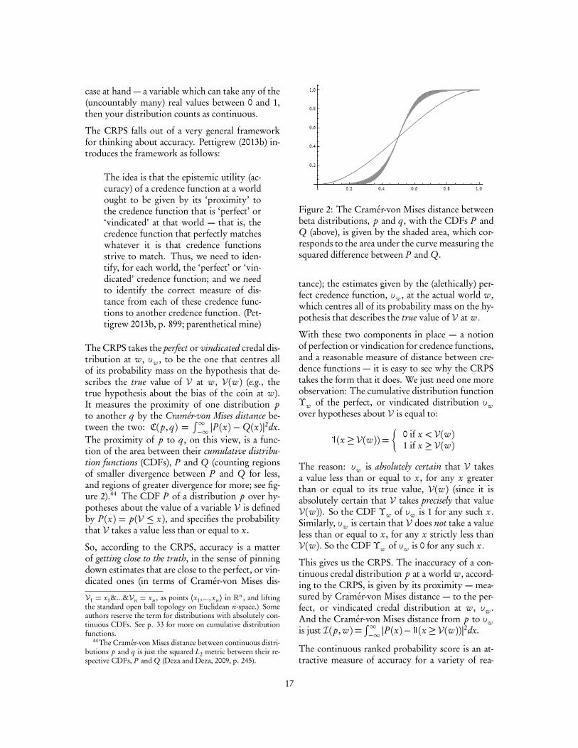
In addition to respecting this insight about thevalue of cognitive skill, it also explains our con-sidered judgments about whether such skill is inplay in a range of cases. Suppose, for example,that a middle aged man comes into the ER withchest pain. Two doctors, Jim and Betsy, observehim. They both have the same prior evidence,let’s imagine (a brief description of the man’s symp-toms, together with background medical knowl-edge). And it fails to discriminate between vari-ous competing hypotheses, e.g., that the patient’schest pain is caused by a heart attack, that it iscaused by hyperventilation, etc. Both Betsy andJim’s prior credences, i.e., credences prior to ac-quiring new clinical data, are consistent with theconstraints imposed by their prior evidence, let’sstipulate. But Jim’s credences also reflect a hunch.He ‘feels it in his bones’ that the patient’s chestpain is a result of hyperventilation, and so lendsmuch more credence to that hypothesis than to theothers. Betsy, on the other hand, spreads her cre-dence much more evenly over all of the relevanthypotheses.

To be clear, Jim is not recognising some ineffablesigns that Betsy is missing (in the way that Dr.House might). If he were, he would have more ev-idence than Betsy, contra our assumption (even ifhe could not express that evidence to anyone). Thebias in Jim’s prior reflects a ‘mere hunch’.

Importantly, concentrated priors like Jim’s arerather resilient with respect to a wide range ofdata.16 Learning something new does not alterthem much (for many new data items). Betsy’sprior, in contrast, is much more malleable, muchmore prone to change in the face of new data. Sowhen Betsy runs her diagnostic tests and updatesher prior, she revises her credences quite a bit. Incontrast, when Jim updates on the same clinicaldata, he revises his credences fairly minimally.

Suppose that Betsy and Jim are both successful.Their updated credences are fairly accurate. Theyboth end up concentrating most of their credence

16A distribution p is resilient with respect to a datum D tothe extent that pD (·) = p(·|D) is close to p. In §5.2, I intro-duce one particularly attractive divergence between distribu-tions: Cramér-von Mises distance, C. If we use Cramér-vonMises distance as our measure of ‘closeness’ when explicatingresilience, then we can say: a distribution p is resilient with re-spect to a datum D to the extent that C(p, pD ) is close to zero.

on the hyperventilation hypothesis, and the pa-tient is, in fact, suffering chest pain as a result ofhyperventilation. But Jim is a little closer to cer-tain. His credences are a little more concentrated.So Jim’s posterior is a little more accurate thanBetsy’s. Still, his success seems to be less a productof cognitive skill than Betsy’s, and more a productof his lucky hunch.

The current account explains this judgment. Be-cause Jim’s prior is biased strongly in favour of thehyperventilation hypothesis (reflecting his hunch),it is fairly resilient with respect to new data. Asa result, his posterior accuracy depends a great dealon his prior accuracy. His high degree of poste-rior accuracy is explained, in no small part, by thefact that his prior credences were quite accurate(his hunch was correct). This is constitutive, onthe proposed account, of failure to manifest cog-nitive skill. Skilled reasoning, on this view, mit-igates the explanatory relevance of non-evidentialfactors, such as fortuitous prior accuracy, so thatthey are no more relevant than required by one’sprior evidence.17

If this is right, then we can recast the probabilisticability condition as follows:

PROBABILISTIC ABILITY CONDITIONÆ.Probabilistic knowledge requires cognitiveability, in the following sense: if some of yourcredences constitute knowledge, then yourevidence explains their success (accuracy) tothe greatest degree possible.

The hope now is to find some way of sifting credalstates that satisfy this ability condition from onesthat do not. My plan is to identify a particular‘summary statistic’ that tracks the amount of cog-nitive ability that a credal state manifests. I willthen use this statistic to develop a novel kind of ob-jective Bayesianism that delivers credences that arenot only reasonably likely to be accurate, in a widerange of cases, but whose accuracy is, to the great-est extent possible, a product of cognitive ability.

17Prior evidence E can require a factor F to be relevant toexplaining posterior accuracy to some degree k in the followingsense: F is relevant to degree k for every prior p in the set ofdistributions S consistent with the constraints imposed by E . Inparticular, E can require prior accuracy to be relevant to degreek, in the following sense: p’s (prior) accuracy is relevant forexplaining the (posterior) accuracy of p ′ to at least degree k, forevery p in S.

7

Such credences are particularly good candidates forprobabilistic knowledge.

4 Chance and Explanation

To identify our summary statistic, we need to saya bit more about how cognitive skill manages tomake evidential factors (how weighty, specific, mis-leading, etc., your evidence is) comparatively im-portant for explaining your success (accuracy), andmake non-evidential factors (lucky hunches, etc.)comparatively unimportant.

Foreshadowing a bit (in an imprecise, but illustra-tive way), here is what we will find: Past facts ex-plain future events always and everywhere by ex-plaining the chances at intervening times. So, ifwiggling the past fact does not make the chanceof the future event wiggle, so to speak, then thepast fact does not explain the future event. This is,more or less, how cognitive skill works its magic. Itmakes it so that wiggling (or altering, in a Lewisiansense) certain past facts — e.g., the fact that a hunchof yours turned out to be spot-on (or wildly-off)— does not wiggle (or alter) the chance of a cer-tain future event — e.g., arriving at accurate cre-dences after performing an experiment, gatheringsome data, and updating on that data.18 And inthat case, the past fact (about prior accuracy) plau-sibly does not explain the future event (attainingposterior accuracy). Facts about the data explainit instead. And this is just what is required for thefuture event to be the product of cognitive skill, onour view.

To fill in the details of this story — about howcognitive skill makes evidential factors importantfor explaining success, and makes non-evidentialfactors unimportant — start by considering an in-structive case involving practical skill:

MARS ROVER. The new Mars rover is beginningits descent through Mars’ atmosphere. At theoutset, it is blind. A bulky heat shield blocksits sensors. But before long it will eject theheat shield, release its supersonic parachute,and slow down a bit. At that point, its sen-

18An alteration of one event is, to a first approximation, an-other event that differs slightly in when or how it occurs. See(Lewis, 2000, p. 188). Altering one event C fails to alter anotherE if the following is true: had any one of a range of alterationsC1, ...,Cn of C occurred, E would have occurred just the same.

sors will make various readings, and it willmanoeuvre its way to the landing site. If therover is equipped with a guidance programthat makes it skilled at landing, then its chanceof success (touching down close to the target)would be (more or less) the same (invariant),whether it happens to emerge from its ini-tial (blind) descent directly above the landingsite, or 3 miles to the north, or 5 miles to thenortheast. Its skill will make it so that (withinreasonable bounds) facts about its initial prox-imity to the site — facts that it has no infor-mation about during the blind part of its de-scent (non-evidential factors) — have little tono impact on its chance of success. As a re-sult, the rover’s initial proximity to the land-ing site will plausibly be irrelevant for explain-ing both (i) why that chance of success is whatit is, and (ii) why it achieves whatever actualdegree of success that it does.

Facts about initial proximity to the landing site arenot reflected in the rover’s total evidence; they donothing to explain the character of that evidence.Initial proximity is, in this sense, a non-evidentialfactor. The rover’s skill at landing makes this sortof non-evidential factor irrelevant twice over.19 Itmakes it irrelevant for explaining why the rover’schance of success is what it is (evidenced by theinvariance of that chance across changes in initialproximity). It also makes it irrelevant for explain-ing why the rover is actually successful to the de-gree that it is (why it actually touches down closeto the target or not). The two are intertwined. Therover’s skill makes initial proximity irrelevant forexplaining actual success exactly by making it irrel-evant for explaining the chance of success. No factcan help explain why the rover actually lands closeto the target without explaining why its chance of

19This is so whether or not conditions on Mars are kindenough for the rover to have a positively high chance of suc-cess (landing near the target). If the conditions on Mars aremassively unpredictable, and the landing task massively com-plex, then our skilled rover might have a low chance of landingwithin, say, 0.5 miles of its landing site. (The Curiosity rover,for example, which was extremely skilled at landing, toucheddown 1.5 miles from its landing site.) Our rover might have amuch lower chance than it would if it blindly and unskilfullyrocketed due north during initial descent, burning resources be-fore its sensors even come online (if it is in fact due south). Still,its skill at landing makes non-evidential factors irrelevant (ornearly irrelevant) for explaining why it achieves the degree ofsuccess that it does in fact achieve.

8

landing close to the target is what it is.

This phenomenon is quite general. Chances areexplanatory foci. Or more carefully: chances arecausal-explanatory foci. No past fact can (causally)explain a future event E except by also (partially)explaining why the chance of E (if defined) takesthe values that it does at intervening times.20,21 (Allthe events of interest to us — touching down neara landing site, diagnosing a patient’s medical con-dition, etc. — have causal explanations. So we cansafely restrict our attention in this way.)

The argument that chances are (causal) explanatoryfoci (summed up informally in just a moment) goesas follows.

1. Suppose event C occurs in the history of some(closed) causal system S prior to the currenttime t , and event E occurs in the history of Safter t . Then any causal influence that C hason E proceeds by influencing S at t .22

2. Moreover, any past fact (any fact about thepre-t history of S) that helps to explain howor why C influences E proceeds by explainingwhy some causally relevant part of S is in thestate that it is at t (or, perhaps, by explainingwhy the laws governing S are what they are).

3. The chance of E at t is determined — andhence explained — by the totality of facts spec-ifying which states the causally relevant partsof S are in at t (together with facts about thelaws governing S).

20A fact F about the past causally explains a future event Eby explaining how or why some past event C causally influ-ences E . Perhaps facts are proper causal relata, as Bennett (1988)and Mellor (1995) maintain. In that case, we might simply say:No past fact can (partially) cause a future event E except by (par-tially) causing the chance of E to take the values that it does atintervening times. But we hope to remain neutral about the na-ture of causal relata. So our original formulation wins the day.Whether or not past facts causally promote future events, theysurely causally explain future events, by explaining why theircausal ancestors were the way they were.

21For our purposes, it will suffice if the possible outcomesof some interesting range of experiments — the results of coinflips, western blots, etc. — are chancy, as the theoretical hy-potheses we typically take to explain those outcomes posit. Inthat case, the events of interest for us — achieving a particulardegree of (posterior) success (accuracy) after conditionalising onthe outcome of an experiment — are also chancy. And in thatcase, our summary statistic will turn out to be a good guide tothe amount of cognitive ability that a credal state manifests, andcan help us secure probabilistic knowledge.

22Premises 1-3 are inspired by (Joyce, 2007, pp. 200-202).

4. So any past fact that helps to explain C ’s influ-ence on E does additional explanatory work:it helps to explain why some causally relevantpart of S is in the state that it is at t (or whythe laws governing S are what they are, by 2),and so helps to explain why the chance of E iswhat it is at t (by 3).

5. No past fact F helps to causally explain Eexcept by explaining how or why some pastevent C influences E .

C. So F helps to causally explain E (in virtue ofexplaining C ’s influence on E , by 5), only if Fhelps to explain why the chance of E is whatit is at t (by 4).

Shorter: past facts causally explain future eventsonly by explaining how or why past events in-fluence those future events; but all causally rel-evant facts of this sort explain why the presentstate is what it is; and any fact that does that alsoexplains why the present chances are what theyare; so chances are causal-explanatory foci; past factscausally explain future events always and every-where by explaining the chances at interveningtimes.

This feature of chance — that it acts an explanatoryfocal point — might seem recherché. But it is actu-ally quite banal. An example will help:

ASTHMA DRUG. You have pretty bad asthma.Your doctor recommends a new drug,BreatheEZ c©. Happily, it clears right up. Afew months later, you stumble across a reportin the Journal of Asthma Studies. The previ-ous clinical trials of BreatheEZ c© were flawed.In more recent trials, it failed to demon-strate a statistically significant increase in pos-itive health outcomes compared to placebo.This, you think, is good evidence that takingBreatheEZ c© failed to affect, or explain in anyway, the patients’ chance of recovery. If tak-ing BreatheEZ c© really was part of the causalstory explaining why their chances were whatthey were, then the new, improved clinical tri-als would have demonstrated a statistically sig-nificant increase in health outcomes.

Now suppose you think that you are just like thosepatients in all of the relevant respects, and concludethat taking BreatheEZ c© does not explain why your

9

chance of recovery was what it was. Then it wouldbe natural to infer that it fails to explain why youactually recovered. Maybe moving to a new citywith different allergens, or something of the sort,explains your recovery. Whatever the right storyis, though, BreatheEZ c© is no part of it. This in-ference is mediated by the chances-as-explanatory-foci thesis. No past fact (the fact that you tookBreatheEZ c©) can help explain one’s success (recov-ering from asthma) without explaining why one’schance of success was what it was.

We will now attempt to leverage this fact aboutchance — that chances are explanatory foci — toidentify a ‘summary statistic’ of credal states thatwill help us sift ones that satisfy the probabilisticability condition from ones that do not. Here ishow we will proceed. Firstly, we will look for astatistic that helps us sort out, for any given credalstate, what explains why its chance of success (pos-terior accuracy) is what it is, in any experimentalcontext. Does it reflect some sort of hunch thatgoes beyond the available prior evidence? A hunchwhich explains why it has a particularly high (orlow) chance of posterior (post-experiment) success?Or is its chance of success (accuracy) explained,rather, by the character of the experimental evi-dence that will be used to update those credences:how weighty it is, how specific it is, etc.?

If we find such a statistic, we will be off to the races.It will help us sort out which factors explain whyany given credal state’s chance of success (posterioraccuracy) is what it is. And because chances are ex-planatory foci, this will enable us to sort out whichfactors explain why that credal state actually attainsthe degree of success that it does. And this is ex-actly what determines whether success (posterioraccuracy) is the product of cognitive ability. So wewill be able to sift credal states that satisfy the prob-abilistic ability condition from ones that do not.

5 Cognitive Ability and ObjectiveExpected Accuracy

5.1 An Example: Scientific Inquiry

To have a concrete case in front of us, while search-ing for our ability-tracking summary statistic,imagine the following. A microbiologist designsand performs an experiment to adjudicate betweencompeting theoretical hypotheses H1, ..., Hn , e.g.,

various hypotheses about whether and how over-expression of a certain gene causes chromosomalinstability in breast tumours. She has certainprior (pre-experiment) credences, c(H1), ..., c(Hn),which reflect both her prior evidence — informa-tion about past patients, about chromosomal insta-bility in other sorts of tumours, and so on — as wellher personal inductive hunches and quirks. Shewill also soon acquire new experimental data D ,which she will use to update her prior credences,to arrive at new, better informed posterior (post-experiment) credences, c ′(H1), ..., c ′(Hn).

For precision, assume that any agent we consider,our microbiologist included, has credences c :Ω→R defined over a Boolean algebra of propositions Ω(closed under negation and disjunction). And foreach atom ω of Ω (each of the finest grained pos-sibilities she can distinguish between), let wω be‘the’ possible world that makesω true. (The differ-ences between worlds that agree on the truth-valueofω do not matter, for our purposes. So we ignorethem. And we drop the subscripts henceforth.) LetW be the set of all such worlds.

Assume also that our agent satisfies some fairly un-controversial epistemic norms. Her credences areprobabilistically coherent.23 She updates by con-ditionalisation, so that, when she acquires a newdatum D (and nothing more), she adopts posteriorcredences c ′ :Ω→Rwhich satisfy c ′(X ) = c(X |D)for all X ∈ Ω.24 And she obeys the Principal Prin-ciple. So she treats chance as an epistemic expert.When she learns that chance’s probability for Xat t is x, she straightaway adopts x as her new

23See Joyce (1998, 2009), Predd et al. (2009), and Schervishet al. (2009) for an accuracy-dominance argument that rationalcredences must be probabilistically coherent, i.e., must satisfythe laws of finitely additive probability:

1. c(>) = 12. c(⊥)≤ c(X )3. c(X1 ∨ ...∨Xn) = c(X1) + ...+ c(Xn) for any pairwise in-

compatible propositions X1, ...,XnAxiom 1 says that you must invest full confidence in tautolo-gies. Axiom 2 says that you must invest at least as much con-fidence in any proposition X as you do a contradiction. Ax-iom 3 says that the amount of confidence that you invest in adisjunction X1 ∨ ...∨Xn of pairwise incompatible propositionsX1, ...,Xn must be the sum of your degrees of confidence in eachof the Xi .

24When c(D) > 0, c(X |D) is just c(X &D)/c(D). For a the-ory of conditional probability that allows c(X |D) to be definedwhen c(D) = 0, see Rényi (1955) and Popper (1959). For anexpected accuracy argument for conditionalisation, see Greaves(2006), Leitgeb and Pettigrew (2010), and Easwaran (2013).

10

credence for X (unless she has information thatchance lacks at t ).25

Finally, make a couple of additional assumptionsabout the propositions in our microbiologist’s al-gebra. She has credences about the competing the-oretical hypotheses H1, ..., Hn that she hopes to ad-judicate between, which we suppose are pairwiseincompatible and jointly exhaustive (they parti-tion W).26 She also has credences about the differ-ent possible experimental outcomes she might ob-serve, or the new data she might receive, D1, ..., Dm(which also partition W). And these two sets ofpropositions are related. Each hypothesis Hi spec-ifies chances for the possible data items D1, ..., Dm .To have a way of talking about them, let chi be thefunction that would specify the chances if Hi weretrue. So the chance that our microbiologist’s exper-iment would yield outcomes D1, ..., Dm if Hi weretrue is chi (D1), ..., chi (Dm), respectively. (This no-tation will be helpful shortly.)

Our question is this: What can we say about the ex-tent to which the character of our microbiologist’sevidence explains the success (accuracy) of her pos-terior credal state (and hence the extent to whichher credences satisfy the probabilistic ability con-

25More carefully, the Principal Principle says:

PRINCIPAL PRINCIPLE. If an agent’s total evi-dence is limited to information about the history ofthe world up to time t , then her credences c oughtto satisfy:

c(X |D&cht (X ) = x) = xprovided c(D&cht (X ) = x) > 0, where D is any‘admissible’ proposition, and cht (X ) = x is theproposition that the chance of X at t is x. (Joyce,2007, p. 196)

According to Lewis (1980, p. 272), “admissible propositions arethe sort of information whose impact on credence about out-comes comes entirely by way of credence about the chances ofthose outcomes.” Historical information, for example, is admis-sible (Lewis, 1980, p. 272); information that “bears in a directenough way on the outcome,” such as testimony about the re-sult of an experiment, is inadmissible (Lewis, 1980, p. 265). Pet-tigrew (2012, p. 4) makes Lewis’ account of admissibility moreprecise.

See Pettigrew (2013b) for a chance-dominance argument forthe Principal Principle. For discussion of alternative deferenceto chance principles, which have certain virtues that the Prin-cipal Principle lacks, see Hall (1994, 2004), Joyce (2007), Ismael(2008), Meacham (2005, 2010) and Pettigrew (2012, 2013b). Forsimplicity, we assume that the agents under consideration lackinadmissible evidence. We also assume that chance is not self-undermining. The differences between these alternatives arenegligible in this case.

26A partition of W is a collection of disjoint subsets of Wwhose union is W .

dition)? Do other factors play a significant explana-tory role? In particular, do her prior credences re-flect some sort of hunch that goes beyond her priorevidence (as Dr. Jim’s did), so that her posteriorsuccess depends, in large part, on fortuitous priorsuccess?

First, we will outline the answer. Then we will un-pack it. The answer, briefly, is this: If her objectiveexpected posterior accuracy would be the same (in-variant), regardless of whether her prior credencesreflect a particularly accurate hunch or not, thenthat hunch plausibly plays no role in explainingwhy her chance of success is what it is. And ifthe accuracy (or inaccuracy) of her hunch does notexplain her chance of success, then it simply can-not explain her actual degree of posterior success.Chances are explanatory foci. So, if her objectiveexpected posterior accuracy would be the same,whether her prior credences reflect a particularlyaccurate hunch or not, then the accuracy of thathunch is plausibly irrelevant for explaining whyshe attains whatever actual degree of posterior suc-cess that she does. Rather, her success is explainedprimarily by the character of her evidence: howweighty, specific, misleading it is, etc. And this isjust what is required for her success to be the prod-uct of cognitive ability.

To unpack this answer, make two observations.

5.2 Observation 1: Accuracy vs. ExpectedAccuracy

Firstly, we can distinguish between the actual ac-curacy of our microbiologist’s prior and posteriorcredences — roughly, how close they are to the ac-tual truth-values — and the objective expected poste-rior accuracy of her credences. A bit of backgroundwill help illuminate what objective expected ac-curacy is and why it is important. Expectationsare estimates.27 More carefully, if V is some (real-valued) random variable — e.g., the annual rainfallin New York, the amount of money in your bankaccount, the degree of inaccuracy of a microbiolo-gist’s credences — then Expp (V) =

∑

w∈W p(w) ·V(w) is the best estimate of V , according to theprobability function p, where V(w) is the valuethat V takes in world w (the annual rainfall in

27See Jeffrey (2004), chapter 4.

11

New York in w, etc.).28 Objective expectations arethe estimates determined by objective probabilityfunctions — the true chance function, in particular.So, for example, if ch is the true chance function,then its best estimate of the annual rainfall R inNew York is just the objective expected value ofR, Expch(R) =

∑

w∈W ch(w) ·R(w).

Similarly, chance’s best estimate of how success-ful our microbiologist will be — how accurateher credences will be after performing the exper-iment, observing the outcome, and updating onher new data — is just her objective expected pos-terior accuracy. Imagine, for example, that Hi isthe true theoretical hypothesis. So chi is the truechance function (just prior to performing the ex-periment). And the chance of the experiment pro-ducing outcomes D1, ..., Dm is chi (D1), ..., chi (Dm),respectively. Now note that updating (condition-ing) her prior credences c on these bits of pos-sible new evidence yields different posterior cre-dence functions, cD1

, . . . , cDm. And each of these

credence functions is (or at least could be) accurateto a different degree. So not only does chance haveviews about which bit of evidence our microbiolo-gist will receive — given by chi (D1), ..., chi (Dm)— italso has views about how likely she is to attain var-ious different degrees of posterior accuracy; viewswhich are summed up by chance’s best estimate ofher success, i.e., her objective expected posterior ac-curacy.

To keep track of these degrees of accuracy, andto say explicitly what our microbiologist’s objec-tive expected posterior accuracy is, let’s introducesome notation. Let I(cD j

, w) be a non-negativereal number which (in some as of yet unspecifiedway) measures the inaccuracy of the posterior cre-dence function cD j

at world w. If I(cD j, w) = 0,

then cD jis minimally inaccurate (maximally close

to the truth) at w. Inaccuracy increases as I(cD j, w)

grows larger. (See §5.2 for an extended discussionof inaccuracy measures.)

Now we can specify the objective expectedposterior accuracy of our microbiologist’s cre-dences: Expchi

(I(c ′)) =∑

D j∈D1,...,Dm chi (D j ) ·

28Random variables V : W → R are functions from worldsW into the real numbers R, which model (measurable) quanti-ties of interest, e.g., the year Turing died.

∑

w∈D jchi (w|D j ) · I(cD j

, w).29,30 This is chi ’s bestestimate of how successful she will be. It sum-marises all of the information that chi sees as rele-vant to what degree of posterior success (accuracy)she will achieve. The closer Expchi

(I(c ′)) is to zero,the more likely she is (all things considered) to besuccessful, according to chi (i.e., to end up with ac-curate post-experiment credences).

5.3 Observation 2: CounterfactualIndependence as a Guide to ExplanatoryIrrelevance

Second observation: Chance’s best estimate of howsuccessful our microbiologist will be — or rather,how that estimate behaves across a range of coun-terfactual scenarios — is a good guide to what isrelevant (and not relevant) for explaining why herchance of success is what it is. Imagine, for exam-ple, that she could perform her experiment usinginstrument A, B or C . If chance’s best estimate ofhow successful she will be — her objective expectedposterior accuracy — would be the same whethershe opted for A, B or C , then which instrumentshe uses plausibly plays no role in explaining whythat expectation is what it is. Counterfactual inde-pendence provides good (but defeasible) evidenceof explanatory irrelevance.31

Moreover, expectations are typically good proxiesfor whole distributions (at least for the purposes ofsorting out what does and does not help to explainone’s chance of success). In many experimentalcontexts, if one’s expected accuracy would stay thesame, were the value of some variable to change —

29I(c ′)(·) is shorthand for I(c ′, ·). So I(c ′) : W→R is a ran-dom variable; a function which maps worlds w to real numbersI(c ′, w). It measures (in some way or other) the inaccuracy ofc ′ at worlds w.

30We assume that D j is the total new evidence that our mi-crobiologist acquires in any world in which her experiment pro-duces outcome D j . So c ′ = cD j

and hence I(c ′, w) = I(cD j, w)

for any w ∈D j .31Counterfactual independence only provides defeasible evi-

dence of explanatory irrelevance, however. Imagine, for exam-ple, that our microbiologist uses high quality growth media Afor her cell culture. If she had used lower quality growth mediaB or C , however, her labmate would have added a supplementthat made it functionally equivalent to A. In that case, using Ahelps to (causally) explain why her expected accuracy is whatit is, even though that expectation would be the same whethershe opted for A, B or C . We ignore cases like this involving pre-emption or trumping in what follows. Such cases are outsidethe domain of applicability of the tools developed here.

12

which instrument our microbiologist uses, for ex-ample — then one’s entire distribution of chancesover accuracy hypotheses (hypotheses about whatdegree of posterior accuracy one achieves) wouldstay the same.32 So we can say: which instrumentshe uses — A, B or C — plausibly plays no role inexplaining why her chance of success is what it is. (Wecould, if we were so inclined, avoid using expecta-tions as proxies. But doing so would be messy, andprovide no additional insight. So the game is notworth the candle.33)

More generally, if chance’s best estimate of yoursuccess — your objective expected posterior accu-racy — would be the same, regardless of what valuesome variable V takes, then V plausibly plays norole in explaining why your chance of success iswhat it is.

Now recall our initial question. We wantedto know whether our microbiologist’s prior cre-dences c reflect some sort of hunch that goes be-yond her prior evidence; a hunch which explainswhy she has a particularly high (or low) chance ofsuccess (posterior accuracy); a hunch which, as aresult, helps explain why she attains whatever ac-tual degree of success that she does. We now havethe tools to sort this out.

32Letting expected accuracy go proxy for the entire distribu-tion of chances over accuracy hypotheses is often harmless.Specifically, when your prior credences over candidate chancefunctions takes the form of a beta distribution (a very flexibleclass of prior distributions; see f.n. 41), and those chance func-tions themselves are binomial distributions (which will be thecase, e.g., when the trials of your experiment are identical andindependent, and yield a sequence of ‘successes’ and ‘failures’),then the distribution over accuracy hypotheses determined byany such chance function can be approximated by an exponen-tial distribution. And it is easy to show that the Cramér-vonMises distance (to take one example) between any two expo-nential distributions is bounded by the difference between theirmeans, or expected values. So objective expected posterior accu-racy is invariant across a range of values for some variable onlyif the entire distribution of chances over posterior accuracy hy-potheses is invariant.

33We could, in principle, directly examine how much one’schance distribution over accuracy hypotheses would vary acrossa range of values for some variable of interest (using an appro-priate metric on the space of probability distributions, suchas Cramér-von Mises distance; cf. §5). This would allow usto avoid the detour through objective expected accuracy alto-gether. But doing so would come at a significant computationalcost (approximating the MaxSen prior in §7 would be infeasi-ble), and would make no difference in the simple cases that weconsider (cf. footnote 32).

5.4 Explaining Posterior Accuracy

Suppose c ’s objective expected posterior accuracywould be the same, whether those prior credencesc reflect a particularly accurate hunch or not;whether the variable of interest for us — prior accu-racy — takes a particularly high or low value. Putdifferently, suppose it would be the same, regard-less of whether the true hypothesis Hi happens tobe one that c initially centres a great deal of prob-ability mass around — in which case c has a highdegree of prior accuracy — or whether the true hy-pothesis H j happens to be one that c centres littlemass around — in which case c has a lower degreeof prior accuracy. More succinctly, suppose:

INVARIANCE. Expchi(I(c ′))≈ Expch j

(I(c ′)) for allHi and H j .

Then we can say: whether c reflects a particularlyaccurate hunch or not (whether c attains a partic-ularly high or low degree of prior accuracy) is ir-relevant for explaining why its chance of posteriorsuccess (accuracy) is what it is.

Finally, recall that chances are explanatory foci.No past fact (e.g., facts about prior accuracy) canexplain a future event (attaining a particular degreeof posterior accuracy) except by (partially) explain-ing why that event had the chance of occurring thatit did. So, since fortuitous prior success (accuracy)is irrelevant for explaining why c ’s chance of pos-terior success (accuracy) is what it is, it is also irrel-evant for explaining why c attains whatever actualdegree of posterior success that it does.

Our microbiologist’s prior credences, then, aremore like Dr. Betsy’s than Dr. Jim’s. Theyare more a product of cognitive skill than a luckyhunch. Because they have a special property (theirobjective expected posterior accuracy is invariantacross theoretical hypotheses) it ends up being thecase (and we can tell a principled story about whyit is the case) that her posterior success does not de-pend on having a fortuitously spot-on prior hunch;a hunch that goes beyond her prior evidence; ahunch which explains why she has a particularlyhigh (or low) chance of success (posterior accu-racy); a hunch which, as a result, helps explain whyshe attains whatever actual degree of success thatshe does. Rather, her success is explained primar-ily by the character of her evidence.

13

This answer to our initial question has variousmoving parts. But once we get a grip on them, thepoint is simple. Consider an analogy. If chance’sbest estimate of how many games Ghana will winin the World Cup — Ghana’s objective expectedwin total — would be the same, regardless of whatcolour socks they decide to wear, then sock colourplausibly plays no role in explaining why theirchance of winning 1, or 2, or 3 games, etc., iswhat it is. And chances are explanatory foci. Sosock colour also plays no role in explaining whythey actually win the number of games that theydo. If chance’s best estimate of how much moneyyou will win playing poker — your objective ex-pected earnings — would be the same, regardless ofwhether you wear oversized sunglasses and a cow-boy hat or not, then wearing those things plausiblyplays no role in explaining why your chance of win-ning $10, or $20, or $30, etc., is what it is. Andchances are explanatory foci. So wearing glassesand a hat also plays no role in explaining why youactually win the amount of money that you do.

Similarly, if chance’s best estimate of how success-ful our microbiologist’s credences will be — herobjective expected posterior accuracy — would bethe same, regardless of how accurate a hunch thosecredences happen to encode, then that hunch plau-sibly plays no role in explaining why her chanceof being accurate to degree x, y, or z is what itis. And chances are explanatory foci. So havinga spot-on (or wildly-off) hunch also plays no rolein explaining why she actually attains the degreeof posterior success (accuracy) that she does. Ourmicrobiologist’s actual degree of posterior successis, rather, explained primarily by the character ofher evidence: how weighty it is, how specific it is,whether or not it is misleading, etc. And this is justwhat is required for her success to be the product ofcognitive ability.

We now have the ‘summary statistic’ of credalstates that we have been looking for; the statis-tic that will help us sift credal states that satisfythe probabilistic ability condition from ones thatdo not. It is: variance in objective expected poste-rior accuracy across theoretical hypotheses. (We willsay more about how to measure variance in §6.)The smaller this statistic, the greater the extent towhich posterior success (accuracy) is a product ofcognitive ability.

My aim now is to use this statistic to help us securenice posterior credences — credences that are notonly reasonably likely to be accurate, but whoseaccuracy is the product of cognitive ability — in awide range of inference problems. Inference prob-lems, of the sort familiar from classical statistics,arise in structured, but nonetheless fairly ubiqui-tous contexts of inquiry (in the sciences, in engi-neering, etc.): we have competing hypotheses wewish to adjudicate between; we will soon acquirenew (experimental) data that we can use (togetherwith our prior data) to help us so adjudicate; andwe know enough about the data-generating pro-cess (the experiment) to know which data itemscould be produced, and what the chances of receiv-ing each of the various possible data items wouldbe, were these different theoretical hypotheses true(typically as a result of careful experimental de-sign). The formal tools developed here will take ussome way toward securing probabilistic knowledgein many of these important contexts of inquiry.

6 The Maximum Entropy Method

6.1 A Case Study

When an agent performs an experiment aimed atadjudicating between competing (pairwise incom-patible and jointly exhaustive) theoretical hypothe-ses, H1, ..., Hn , she should, according to one popu-lar brand of objective Bayesianism — the maximumentropy method, or MaxEnt — take her prior infor-mation into account as follows:

• Firstly, she should summarise that prior infor-mation by a system of constraints, e.g.:

– Hi is at least as probable as H j

– Hi is probable to at least degree 0.6 andat most 0.9

– Hi conditional on D is at least as proba-ble as H j conditional on D ′

which we model by a set of credence functionsC (viz., the set of all credence functions thatsatisfy those constraints).

• Secondly, she should adopt some prior c orother that maximises Shannon entropy over

14

C (which, under a broad range of conditions,will turn out to be unique).34,35

If she has no prior information about H1, ..., Hn atall — her evidence fails to constrain her prior cre-dences altogether — then the maximum entropydistribution is just the uniform distribution.36 SoMaxEnt agrees with Laplace’s Principle of Indiffer-ence:

POI. If an agent has no information about hy-potheses H1, ..., Hn , and so no reason to thinkthat any one is more or less probable than anyother, then she ought to be equally confidentin each: c(Hi ) = c(H j ) for all Hi and H j .

Indeed, we can think of MaxEnt generally as mak-ing the same sort of recommendation as POI. POIsays that in one special case — when your evidenceimposes no constraints on your credences — thosecredences should be uniform. MaxEnt says that inall cases your credences should be as close to uni-form as possible, while satisfying the constraintsimposed by your prior evidence.37

34If the credence functions c in C are defined over onlyfinitely many theoretical hypotheses Hx in H, then their ‘en-tropy’ or ‘uninformativeness’, on the MaxEnt approach, is mea-sured by their Shannon entropy, H (c)= –

∑

x c(Hx ) · log(c(Hx )).If they are defined over uncountably many theoretical hypothe-ses, it is standardly measured by their differential entropy, h(c)=–∫

H c(Hx ) · log(c(Hx ))dx.35Since Shannon entropy H is a continuous, strictly convex,

real-valued function, there will be a unique MaxEnt prior when-ever C is a closed, bounded, convex set. This will be the case, forexample, when the agent’s prior evidential constraints specify a(closed) range of expected values for some number of variables(the expected annual rainfall in New York is between 30 and 60inches (inclusive); the expected price of Tesla’s stock at the endof the quarter is between 210 and 230 (inclusive); etc.). Whenthere is no unique MaxEnt prior — either because many priorsmaximise entropy, or because none do — objective Bayesianssuch as Jon Williamson (2010) recommend adopting some prioror other with “sufficiently high” entropy, where what counts assufficiently high depends on various pragmatic considerations.

36More carefully, when our evidence provides no constraintson prior credences c : Ω→ R, and there exists a countably addi-tive uniform distribution on Ω, then the MaxEnt distribution isjust the uniform distribution. In certain contexts, however, theMaxEnt prior exists while a countably additive uniform priordoes not. It is well known, for example, that if Ω is an infinite-dimensional space, then there is no Lebesgue measure onΩ, andhence, no analogue of the standard uniform distribution on Ω.But there is often a MaxEnt prior on such Ω. See, for example,Furrer et al. (2011).

37If c uniquely maximises Shannon entropy over C, then it isas close as possible to the uniform distribution u in the follow-

Jaynes offered an information-theoretic rationalefor MaxEnt. Shannon entropy, Jaynes thought, isuniquely reasonable as a measure of the informa-tiveness of a prior. So “the maximum-entropy dis-tribution may be asserted for the positive reasonthat it is... maximally noncommittal with regard tomissing information,” he concluded (Jaynes, 1957,p. 623). But many find this argument uncom-pelling.38 We will explore, briefly, whether Max-Ent has an alternative rationale — whether it deliv-ers credences that are eligible candidates for consti-tuting probabilistic knowledge.

Imagine that a bookie hands you and your frienda coin, and offers you a bet. Neither of you haveany prior evidence about the coin’s bias. But youare allowed to flip the coin for a bit before decid-ing whether or not to take the bet — 14 times,perhaps. You adopt the maximum entropy prior,which given your dearth of evidence is just theuniform distribution u. So you spread your cre-dence evenly over the various competing hypothe-ses about the bias of the coin — hypotheses of theform B = x (read: the coin’s bias B is x).39

Your friend, in contrast, adopts a more concen-trated distribution b (e.g., a beta distribution withα = 10 and β = 4, which centres most of its prob-ability mass around the hypothesis B = 5/7; seefigure 1).40 Your friend’s prior credences, as a re-

ing sense: for any other b ∈ C, the Kullback-Leibler divergenceof u from b , DKL(b , u) =

∑

w b (w) · log(b (w)/u(w)), is greaterthan the KL divergence of u from c .

38See for example Seidenfeld (1986) and Joyce (2009, pp. 284-5).

39More carefully, your credences over hypotheses about thebias of the coin B are given by u(s ≤ B ≤ t ) =

∫ ts f (x)dx (0 ≤

s < t ≤ 1), where f is the uniform probability density functionf , i.e., the function that assigns the same probability density toeach hypothesis B = x (0≤ x ≤ 1), viz., f (x) = 1.

A distribution u’s density function f , intuitively, centresmore mass (or density) on hypotheses that u sees as more plausi-ble. The probability that u assigns to the true hypothesis beingin some set S is equal to the volume under f on that region S(which is higher the more mass u attaches to hypotheses in S).

40Beta distributions b are parameterised by two quantities,α and β. These ‘shape parameters’ determine which hypothe-ses B = x the distribution b focuses its probability mass on.The ‘concentration parameter’, α+β, corresponds roughly tohow ‘peaked’ b is around its mean. The larger (smaller) α iscompared to β, the more b focuses probability mass on B = xwith x ≈ 1 (x ≈ 0). Beta distributions are fairly computation-ally tractable, and form a very flexible class of distributions. Infact, any prior can be approximated by a mixture of beta distri-butions (Walley, 1991, p. 9). And beta distributions have nicedynamic properties as well. For example, they continue to bebeta distributions when updated on various sorts of data (they

15

sult (like Dr. Jim’s in §2), are rather resilient withrespect to a wide range of data. Flipping the coina few times and observing its outcome does notalter them much.41 In contrast, your prior cre-dences (like Dr. Betsy’s) are much more malleable,much more prone to change in the face of new data.When you flip the coin and observe its outcome,you revise your credences quite a bit.

Figure 1: u and b .

The upshot: your friend’s success — whatever de-gree of posterior accuracy she actually ends upwith after flipping the coin and observing its out-come — seems to be more a product of her lucky(or unlucky) hunch (viz., that the coin’s bias is ap-proximately 5/7) than yours. It is less a product ofcognitive skill.

Our summary statistic bears this out, as we willdemonstrate shortly. Here is what we will show.Chance’s best estimate of how successful u willbe — u’s objective expected posterior accuracy —varies fairly minimally across chance hypothesesB = x: much less than b ’s. It would take nearlythe same value, regardless of how accurate a hunchu happens to encode (regardless of whether the truehypothesis ends up being one that makes u have arelatively high degree of prior accuracy or not). Sohaving a spot-on (or wildly-off) hunch about thecoin’s bias plays less of a role in explaining whyyour chance of posterior success (accuracy) is whatit is. Consequently, it plays less of a role in explain-ing why you actually attain the degree of posteriorsuccess that you do. Your success is explained, to amuch greater degree, by the character of your ev-

are conjugate priors to the binomial, negative binomial and ge-ometric likelihood functions). For these reasons, we will focuson them in many of our examples.

41See footnote 49 for an illustration of b ’s resilience.

idence: how many times you flip the coin (howweighty your evidence is), whether the frequencyof heads in your sequence of coin flips ends up be-ing close to the coin’s true bias (how misleadingyour evidence is), etc. And this is just what is re-quired for your success to be more a product ofcognitive ability than your friend’s.

For concreteness, let’s measure (in)accuracy by anepistemic scoring rule or inaccuracy score. An in-accuracy score is a function I, which maps cre-dence functions c and worlds w to non-negativereal numbers, I(c , w). I(c , w) measures how inac-curate c is if w is actual. If I(c , w) equals zero, thenc is minimally inaccurate (maximally close to thetruth) at w. Inaccuracy increases as I(c , w) growslarger.

Reasonable inaccuracy scores satisfy a range of con-straints (see Joyce (1998, 2009) and Predd et al.(2009)). But instead of detailing these constraints,we will simply focus our attention on a particu-larly attractive inaccuracy measure: the continuousranked probability score (CRPS).42 Readers that areuninterested in the details of the CRPS (which arepretty formal), or the reasons for focusing on it,can skip ahead to §5.3.

6.2 Continuous Ranked Probability Score

The inaccuracy of a continuous credal distributionp over hypotheses about the value of a variable V(e.g., hypotheses about the bias of a coin), relativeto a world w, according to the CRPS, is given by:

(CRPS) I(p, w) =∫∞−∞ |P (x)−1(x ≥ V(w))|2dx

Before explaining this, a bit of terminology. Yourcredal distribution is continuous when you havecredences about the values of variables which cantake uncountably many values (rather than cre-dences about, e.g., a finite number of propositions,which take only two values: 1 at worlds where theyare true, and 0 where false).43 So if you have cre-dences about the bias of a coin — as you do in the

42For discussion of scoring rules for continuous distribu-tions, and the CRPS in particular, see (Gneiting and Raftery,2007, §4).

43Strictly speaking, a distribution p : Ω→ R over hypothe-ses about the values of variables V1, ...,Vn is called continuouswhen its cumulative distribution function P :Ω→R is continu-ous. (The notion of continuity in play here is the standard topo-logical notion. The relevant topology on Ω is just the topologygenerated by modelling the atoms of Ω, which take the form

16

case at hand — a variable which can take any of the(uncountably many) real values between 0 and 1,then your distribution counts as continuous.

The CRPS falls out of a very general frameworkfor thinking about accuracy. Pettigrew (2013b) in-troduces the framework as follows:

The idea is that the epistemic utility (ac-curacy) of a credence function at a worldought to be given by its ‘proximity’ tothe credence function that is ‘perfect’ or‘vindicated’ at that world — that is, thecredence function that perfectly matcheswhatever it is that credence functionsstrive to match. Thus, we need to iden-tify, for each world, the ‘perfect’ or ‘vin-dicated’ credence function; and we needto identify the correct measure of dis-tance from each of these credence func-tions to another credence function. (Pet-tigrew 2013b, p. 899; parenthetical mine)

The CRPS takes the perfect or vindicated credal dis-tribution at w, υw , to be the one that centres allof its probability mass on the hypothesis that de-scribes the true value of V at w, V(w) (e.g., thetrue hypothesis about the bias of the coin at w).It measures the proximity of one distribution pto another q by the Cramér-von Mises distance be-tween the two: C(p, q) =

∫∞−∞ |P (x) −Q(x)|2dx.

The proximity of p to q , on this view, is a func-tion of the area between their cumulative distribu-tion functions (CDFs), P and Q (counting regionsof smaller divergence between P and Q for less,and regions of greater divergence for more; see fig-ure 2).44 The CDF P of a distribution p over hy-potheses about the value of a variable V is definedby P (x) = p(V ≤ x), and specifies the probabilitythat V takes a value less than or equal to x.

So, according to the CRPS, accuracy is a matterof getting close to the truth, in the sense of pinningdown estimates that are close to the perfect, or vin-dicated ones (in terms of Cramér-von Mises dis-

V1 = x1&...&Vn = xn , as points ⟨x1, ..., xn⟩ in Rn , and liftingthe standard open ball topology on Euclidean n-space.) Someauthors reserve the term for distributions with absolutely con-tinuous CDFs. See p. 33 for more on cumulative distributionfunctions.

44The Cramér-von Mises distance between continuous distri-butions p and q is just the squared L2 metric between their re-spective CDFs, P and Q (Deza and Deza, 2009, p. 245).

Figure 2: The Cramér-von Mises distance betweenbeta distributions, p and q , with the CDFs P andQ (above), is given by the shaded area, which cor-responds to the area under the curve measuring thesquared difference between P and Q.

tance); the estimates given by the (alethically) per-fect credence function, υw , at the actual world w,which centres all of its probability mass on the hy-pothesis that describes the true value of V at w.

With these two components in place — a notionof perfection or vindication for credence functions,and a reasonable measure of distance between cre-dence functions — it is easy to see why the CRPStakes the form that it does. We just need one moreobservation: The cumulative distribution functionΥw of the perfect, or vindicated distribution υwover hypotheses about V is equal to:

1(x ≥ V(w)) =

0 if x < V(w)1 if x ≥ V(w)

The reason: υw is absolutely certain that V takesa value less than or equal to x, for any x greaterthan or equal to its true value, V(w) (since it isabsolutely certain that V takes precisely that valueV(w)). So the CDF Υw of υw is 1 for any such x.Similarly, υw is certain that V does not take a valueless than or equal to x, for any x strictly less thanV(w). So the CDF Υw of υw is 0 for any such x.

This gives us the CRPS. The inaccuracy of a con-tinuous credal distribution p at a world w, accord-ing to the CRPS, is given by its proximity — mea-sured by Cramér-von Mises distance — to the per-fect, or vindicated credal distribution at w, υw .And the Cramér-von Mises distance from p to υwis just I(p, w) =

∫∞−∞ |P (x)−1(x ≥ V(w))|2dx.

The continuous ranked probability score is an at-tractive measure of accuracy for a variety of rea-

17

sons. It is extensional. The accuracy of a credaldistribution over hypotheses about the value of avariable V is a function exclusively of (i) the var-ious estimates it encodes — of the truth-values ofthose hypotheses, and of V itself — and (ii) theactual values of those quantities.45 How justi-fied that credal distribution is, in light of somebody of evidence, how reliably produced it is, etc.,makes no difference to its accuracy, according tothe CRPS, except insofar as they help to determinehow close its estimates are to the actual values ofthose quantities. The CRPS is truth-directed. Mov-ing your credences uniformly closer to the truth(while remaining coherent) always improves accu-racy.46 It is strictly proper. Any (coherent) contin-

45It is worth noting that two distributions p and q might doequally well estimating the truth-values of hypotheses about thevalue of V , intuitively, and yet have different inaccuracy scoresaccording to the CRPS, in virtue of encoding different estimatesfor V itself. For example, let V be the bias of the coin, and p andq be distributions that spread their probability mass uniformlyover the ranges [0.3,0.4] and [0.4,0.5], respectively. That is, thedensity function function that defines p, fp , attaches the samepositive probability mass (=10) to any hypothesis V = x withx ∈ [0.3,0.4], and probability mass 0 to every other hypothesis.Similarly for q (mutatis mutandis). Now suppose that the truebias of the coin is 0.6. The value of V at the actual world w is0.6. Then p and q seem to do equally well estimating the truth-values of hypotheses about the value of V . They each spreadtheir probability mass uniformly over sets of equal Lebesguemeasure — sets containing only false hypotheses — and con-sequently attach no probability mass to the true hypothesis,V = 0.6. Yet, p’s best estimate of V , Expp (V) = 0.35, is furtherfrom V ’s true value, 0.6, than q’s best estimate, Expq (V) = 0.45.The CRPS treats this fact as relevant to the accuracy of p and q :I(p, w)≈ 0.233 and I(q , w)≈ 0.133.

This is a feature of the CRPS, not a bug. It is precisely to yieldaccuracy assessments that are “sensitive to distance” in this way— assessments that “give credit” to a distribution for determin-ing a best estimate (expectation) that is close to the true valueof the variable by “assigning high probabilities to values nearbut not identical to the one materializing” — that statisticianssometimes opt for scores like the CRPS, rather than the pre-dictive deviance score, or the ignorance score, etc. (Gneitingand Raftery, 2007, pp. 365-367). This is precisely the reasonthey deem it “more compelling to define scoring rules directlyin terms of predictive cumulative distribution functions,” as theCRPS does, rather than in terms of predictive densities (Gneit-ing and Raftery, 2007, p. 365).

46More carefully, the CRPS is truth-directed in the followingsense: if p and q are both probabilistically coherent, continu-ous distributions over hypotheses about the value of a variableV , and (i) |p(V ∈ S)−w(V ∈ S)| ≤ |q(V ∈ S)−w(V ∈ S)| for allS ⊆R, and (ii) |p(V ∈ S ′)−w(V ∈ S ′)|< |q(V ∈ S ′)−w(V ∈ S ′)|for some S ′ ⊆ R, then (iii) I(p, w) < I(q , w). This is weakerthan the notion of truth-directedness found in (Joyce, 2009, p.269), which applies unrestrictedly, not simply to coherent dis-tributions. But the CRPS is not defined for incoherent distri-butions, and so should not be expected to satisfy Joyce’s more

uous credal distribution expects itself to be moreaccurate than any other distribution (Gneiting andRaftery, 2007, p. 367).47 Perhaps most telling, itis a natural extension of the Brier score, B(p, w)= (1/n) ·

∑ni=1 |p(Hi )−w(Hi )|2 — a paradigmati-

cally reasonable scoring rule for discrete distribu-tions — to the space of continuous distributions(cf. Joyce (2009, §12) and Gneiting and Raftery(2007, p. 365)).48 It also yields the correct verdictabout comparative accuracy in those cases whereobviously correct answers are to be had.49

6.3 Case Study Continued

The bookie hands you and your friend the coin.You adopt the uniform credal distribution u overhypotheses about the coin’s bias B . Your friendadopts a more concentrated distribution b (figure3). Now imagine that the true bias of the coin is5/7. The value of B at the actual world w@ is 5/7.Imagine also that when you flip the coin your allot-ted 14 times, it comes up heads 10 times and tails4. So your new data D is perfectly non-misleading.The true bias of the coin is exactly the frequencyof heads in D , viz., 5/7.

When you and your friend condition on your newdata D , the two of you arrive at the posteriorsu ′ = uD and b ′ = bD , respectively (figure 4). Theresult: your friend is more successful. Her pos-terior is more accurate than yours: I(u ′, w@) =0.028 > 0.020 = I(b ′, w@). But her success is lessa product of cognitive ability than yours.

The reason, informally, is that your friend’s cre-

general truth-directedness constraint.47For more on propriety, which goes under various names

in the literature, see the discussion of cogency in (Oddie, 1997,§3), the discussion of self-recommendation in (Greaves, 2006,§3), and the discussion of propriety in (Joyce, 2009, §8).

48Discrete distributions are non-continuous. Your credal dis-tribution is discrete when you only have credences about count-ably many variables, which can only take countably many val-ues. So, for example, if you have credences about a finite num-ber of propositions, which can take only two discrete values (1at worlds where they are true, and 0 where false), then yourdistribution itself counts as discrete.

49For example, if p and q are beta distributions with the samemean x, but increasing variance, then p is more accurate thanq at a world w where the true value of V is x, according tothe CRPS: I(p, w) < I(q , w). Similarly, if p and q are betadistributions with the same variance, but their means — x and y,respectively — are such that x < y < z, then q is more accuratethan p at a world w ′ where the true value of V is z: I(q , w ′)<I(p, w ′).

18

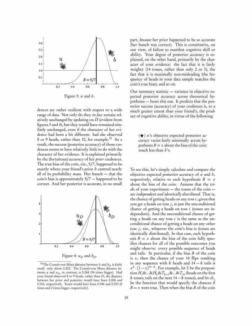
Figure 3: u and b .

dences are rather resilient with respect to a widerange of data. Not only do they in fact remain rel-atively unchanged by updating on D (evident fromfigures 3 and 4), but they would have remained sim-ilarly unchanged, even if the character of her evi-dence had been a bit different: had she observed8 or 9 heads, rather than 10, for example.50 As aresult, the success (posterior accuracy) of those cre-dences seems to have relatively little to do with thecharacter of her evidence. It is explained primarilyby the (fortuitous) accuracy of her prior credences.The true bias of the coin, viz., 5/7, happened to beexactly where your friend’s prior b centred nearlyall of its probability mass. Her hunch — that thecoin’s bias is approximately 5/7 — happened to becorrect. And her posterior is accurate, in no small

Figure 4: uD and bD .

50The Cramér-von Mises distance between b and bD is fairlysmall: only about 0.002. The Cramér-von Mises distance be-tween u and uD , in contrast, is 0.068 (34 times bigger). Hadyour friend observed 8 or 9 heads, rather than 10, the distancebetween her prior and posterior would have been 0.006 and0.016, respectively. Yours would have been 0.046 and 0.033 (8times and 2 times bigger, respectively).

part, because her prior happened to be so accurate(her hunch was correct). This is constitutive, onour view, of failure to manifest cognitive skill orability. Your degree of posterior accuracy is ex-plained, on the other hand, primarily by the char-acter of your evidence: the fact that it is fairlyweighty (14 tosses, rather than only 2 or 3), thefact that it is maximally non-misleading (the fre-quency of heads in your data sample matches thecoin’s true bias), and so on.

Our summary statistic — variance in objective ex-pected posterior accuracy across theoretical hy-potheses — bears this out. It predicts that the pos-terior success (accuracy) of your credences is, to amuch greater extent than your friend’s, the prod-uct of cognitive ability, in virtue of the following:

(Æ) u’s objective expected posterior ac-curacy varies fairly minimally across hy-potheses B = x about the bias of the coin:much less than b ’s.

To see this, let’s simply calculate and compare theobjective expected posterior accuracy of u and b ,respectively, relative to each hypothesis B = xabout the bias of the coin. Assume that the tri-als of your experiment — the tosses of the coin —are independent and identically distributed. That is,the chance of getting heads on any toss i , given thatyou get a heads on toss j , is just the unconditionalchance of getting a heads on toss i (tosses are in-dependent). And the unconditional chance of get-ting a heads on any toss i is the same as the un-conditional chance of getting a heads on any othertoss j , viz., whatever the coin’s bias is (tosses areidentically distributed). In that case, each hypoth-esis B = x about the bias of the coin fully spec-ifies chances for all of the possible outcomes youmight observe: every possible sequence of headsand tails. In particular, if the bias B of the coinis x, then the chance of your 14 flips resultingin any sequence with k heads and 14 − k tails isxk · (1− x)14−k . For example, let S be the proposi-tion H1&...&Hk&Tk+1&...&T14 (heads on the firstk tosses, tails on the next 14− k tosses), and let chxbe the function that would specify the chances ifB = x were true. Then when the bias B of the coin

19

is x, the chance of S is:

chx (S)=chx (H1&...&T14)=chx (H1|H2&...&T14) (Axioms of Probability)· chx (H2|H3&...&T14) · ... · chx (T14)

=chx (H1) · ... · chx (T14) (Independence)

=xk · (1− x)14−k (Identically Distributed)

And the chance of your 14 flips resulting in somesequence or other with k heads and 14− k tails —call this proposition Dk — is:

chx (Dk ) =14

k

· xk · (1− x)14−k

The propositions D0, ..., D14 are the possible newdata items you might receive (and are mutually ex-clusive and jointly exhaustive). They capture allof the information you might learn — how manytimes the coin came up heads and tails, respectively— that is relevant to adjudicating between hypothe-ses about the bias of the coin. (The order of headsand tails, and so on, is irrelevant. The number ofheads is what statisticians call a ‘sufficient statis-tic’.)

Now recall that updating (conditioning) yourprior credences u on these bits of new evi-dence yields different posterior credence functions,uD0

, . . . , uDk, each of which is (or at least could be)

accurate to a different degree. And since chance hasviews about which of these data items you will re-ceive, it also has views about how likely you are toattain these different degrees of posterior accuracy.

Figure 5: The objective expected posterior accu-racy of u across hypotheses B = x.

These views are summed up by u’s objective ex-pected posterior accuracy — chance’s best estimateof how successful u will be — which we can nowcalculate as follows:51

Expchx(I(u ′))

=14∑

k=0

∑

w∈Dk

chx (w)I(uDi, w)

=14∑

k=0

∑

w∈Dk

chx (w)∫ ∞

−∞|UDi(y)−1(y ≥ B(w))|2dy

=14∑

k=0

∑

w∈Dk

chx (w)∫ ∞

−∞|UDi(y)−1(y ≥ x)|2dy

=14∑

k=0

chx (Dk )∫ ∞

−∞|UDi(y)−1(y ≥ x)|2dy

=14∑

k=0

14

k

xk (1− x)14−k∫ ∞

−∞|UDi(y)−1(y ≥ x)|2dy

The mathematical details are not terribly impor-tant. What is important is that we have a well-motivated, concrete way of measuring chance’sbest estimate of how successful u will be if the biasB of the coin is x. So we can examine how muchthis best estimate — u’s objective expected poste-rior accuracy — varies across hypotheses about thecoin’s bias. And, as it turns out, it varies fairly min-imally, as figure 5 shows. This tells us somethingimportant about what explains your success (poste-rior accuracy), and in turn, the amount of cognitiveability that your credal state manifests.

The story — of what explains your success and why— is familiar by now. Suppose chance’s best esti-mate of how successful your credences u will be— your objective expected posterior accuracy —would be the same, regardless of how accurate ahunch those credences happen to encode. That is,suppose u satisfies:

INVARIANCE. Expchx(I(u ′)) = Expchy

(I(u ′)) forall 0≤ x, y ≤ 1.

51Line 3 of the derivations assumes the following: had thebias B of the coin been x (immediately prior to flipping thecoin), there would have been no chance (at just that time) ofthe coin having some other bias y. That is, the function chxthat would specify the chances had B been x attaches zero prob-ability to any world w such that B(w) 6= x.

20

(Your uniform credences u do not perfectly satisfythis supposition. Other prior credences, as we willsee in §6, vary less across hypotheses B = x aboutthe bias of the coin. But they come pretty close:Expchx

(I(u ′)) is roughly 0.065 for all B = x.) Thenthe accuracy of that hunch is (more or less) irrel-evant for explaining why your chance of being ac-curate to any particular degree x, y, or z is whatit is. And chances are explanatory foci. So havinga spot-on (or wildly-off) hunch also plays no rolein explaining why you actually attain the degreeof posterior success (accuracy) that you do (viz.,I(u ′, w@) ≈ 0.028). Your actual degree of poste-rior success is explained, rather, by the character ofyour evidence: the fact that it is fairly weighty (14tosses, rather than only 2 or 3), the fact that it ismaximally non-misleading (the frequency of headsin your data — 5/7 — matches the coin’s true bias),and so on. And this is just what is required for yoursuccess to be the product of cognitive ability.

Your situation mirrors the Mars rover’s in manyways. Suppose that chance’s best estimate of howsuccessful the rover will be — its objective expecteddistance from the landing site — would be thesame, regardless of whether it happens to emergefrom its initial (blind) descent directly above thesite, or 1/2 mile to the north, or 3/4 miles to thenortheast, etc. (Even the fanciest Mars rover doesnot perfectly satisfy this supposition. But in virtueof the actual Mars rover’s skill at landing, it comespretty close.) Then its initial proximity to the land-ing site (a non-evidential factor) is (more or less)irrelevant for explaining why its chance of landingwithin 1, or 2, or 3 miles of that site, etc., is whatit is. And chances are explanatory foci. So initialproximity is also irrelevant for explaining why itattains the actual degree of success that it does —why it actually lands close to its target (or not).

Your friend, however — the one who adopts themore biased beta prior b — is in a different boat.Her prior’s objective expected posterior accuracyvaries rather significantly across hypotheses B = xabout the bias of the coin (figure 6). So the fact thatshe happened to have such a high chance of success(such a low chance of posterior inaccuracy) is ex-plained, in no small part, by the fact that the truebias of the coin, viz., 5/7, happened to be exactlywhere her prior b centred nearly all of its proba-bility mass. It is explained, in no small part, by thefact that her hunch — that the coin’s bias is approx-

Figure 6: The objective expected posterior accu-racy of b from the perspective of chance hypothe-ses H of the form B = x.

imately 5/7 — happened to be correct. Having aspot-on hunch, then, also plays a significant rolein explaining why she actually attains the degreeof posterior success (accuracy) that she does (viz.,I(u ′, w@)≈ 0.020).

Her situation is like a less skilled rover’s. A lessskilled rover might emerge from its initial descentdirectly above its landing site. And its landing strat-egy might give it a high chance of success in thatcase. So it might land close to its target. Still, un-like the skilled Mars rover, its objective expecteddegree of success varies significantly across changesin initial proximity. How close it happens to beto the landing site after emerging from its initial(blind) descent makes a big difference to its chanceof success. The upshot: non-evidential factors(facts about initial proximity) are relevant for ex-plaining why its chance of success is what it is. Inturn, they are relevant for explaining why it is suc-cessful to the degree that it is (why it lands close toits target or not).

This all serves to highlight an important virtue ofMaxEnt. The success (accuracy) of its credencesare, to a large extent, the product of cognitive abil-ity: much more so than the success of various moreconcentrated priors. That success is explained pri-marily by facts about the evidence that it was con-ditioned on — how weighty it is, how specific itis, how misleading it is, etc. — rather than, e.g.,the success or failure (accuracy or inaccuracy) of aprior hunch (a non-evidential factor). And this isjust what is required for success to be the productof cognitive ability. So MaxEnt does seem to de-

21

liver credences that are eligible candidates for con-stituting probabilistic knowledge (at least in sim-ple inference problems). But they are not maxi-mally eligible, I will argue. An alternative objec-tivist method, the MaxSen method, delivers bettercandidates.

7 The MaxSen Method

According to the maximum sensitivity, or MaxSenmethod, when an agent performs an experimentaimed at adjudicating between competing (pairwiseincompatible and jointly exhaustive) theoreticalhypotheses, H1, ..., Hn , she should take her priorinformation into account as follows:

• Firstly, she should summarise that prior infor-mation by a system of constraints, e.g.:

– Hi is at least as probable as H j

– Hi is probable to at least degree 0.6 andat most 0.9

– Hi conditional on D is at least as proba-ble as H j conditional on D ′

which we model by a set of credence functionsC (viz., the set of all credence functions thatsatisfy those constraints).

• Secondly, she should adopt some prior c orother that minimises

var(c) =maxi Expchi(I(c ′)) - min j Expch j

(I(c ′))

over C (which, under a broad range of condi-tions, will turn out to be unique).52

52In particular, suppose that I satisfies two constraints,which we might call worst-case expected convexity and best-caseexpected concavity:

(WCE-Convexity) maxi Expchi(I(c ′)) < λ · [max j

Expch j(I( f ′))]+ (1−λ) · [maxk Expchk

(I(g ′))], for

any c = λ · f +(1−λ) · g with 0< λ< 1.(BCE-Concavity) mini Expchi

(I(c ′)) > λ · [min j

Expch j(I( f ′))]+ (1−λ) · [mink Expchk

(I(g ′))], for

any c = λ · f +(1−λ) · g with 0< λ< 1.

The idea behind WCE-Convexity is that if c strikes some sortof compromise between f and g (c is a mixture of f and g :c = λ · f +(1−λ) · g ), then the worst case of the less compromis-ing distributions f and g (i.e., the estimates of their respectiveinaccuracies determined by the chance distributions that see fand g as most hopeless) should be, on balance, worse than thatof the compromise c . Similarly, the idea behind BCE-Concavity

MaxSen first says that your prior credences oughtto satisfy the constraints imposed by your prior ev-idence E . This bit is common to all kinds of ob-jective Bayesianism, including MaxEnt. You mightprecisify and rationalise it in any number of ways.For example, you might identify C with the set ofcredal states that are best justified in light of E (orweaker: not less justified than some other state, i.e.,either more justified than other states, equally jus-tified, or not ranked in terms of comparative jus-tification). And if you are (as I am) inclined tothink of accuracy as the cardinal epistemic good,and all other good-making features of credences asvaluable primarily in service of the pursuit of accu-racy, you might also endorse the following:

JUSTIFICATION PRINCIPLE. Credal state b isbetter justified than credal state b ∗ in light ofprior evidence E when the objective expected(prior) accuracy of b is higher than b ∗, rela-tive to any chance function ch consistent withE .53 (Cf. Joyce (2013))

Understood in this way, the injunction to satisfythe constraints imposed by your prior evidenceguarantees that your priors are reasonably likelyto be accurate, in light of your prior evidence (orat least not expected to be less accurate than somealternative credal state by all the chance functionsconsistent with your evidence).

MaxSen then says that, from amongst the cre-dences that satisfy the constraints imposed by yourprior evidence, you ought to select the prior thatminimises variance in objective expected posterioraccuracy across the theoretical hypotheses under

is that the best case of the less compromising distributions f andg should be, on balance, better than that of the compromise c .Compromise has both an alethic cost and a benefit, which arereflected in worst and best case objective expected inaccuracies.

When I satisfies these two constraints (and is continuous),var is a continuous, strictly convex, real-valued function. Andany such function takes a unique minimum on any closed,bounded, convex set C. Moreover, C will be closed, boundedand convex in a broad range of circumstances, e.g., when theagent’s prior evidential constraints specify a (closed) range ofexpected values for some number of variables (cf. footnote 33).Specifying what to do when there is no unique MaxSen prioris beyond the purview of our project. The aim, recall, is notto provide the definitive set of formal tools for choosing priorcredences, but rather, to illustrate one kind of tool for securingprobabilistic knowledge in a range of inference problems.

53The Justification Principle only identifies a sufficient condi-tion for b ’s being better justified than b ∗ in light of E . Nonethe-less, it gives us some grip on the contents of C.

22

investigation. This bit is unique to MaxSen. Themotivation for minimising variance is familiar: Ifchance’s best estimate of how successful your cre-dences will be — your objective expected posterioraccuracy — would be the same, or invariant, re-gardless of how a certain non-evidential factor be-haves — fortuitous prior accuracy, in particular —then that factor plausibly plays no role in explain-ing why your chance of being accurate to degree x,y, or z is what it is. And chances are explanatoryfoci. So it also plays no role in explaining why youactually attain the degree of posterior success (accu-racy) that you do.

Selecting prior credences by minimising variance,then, will yield posterior credences whose success(accuracy) is explained, as much as possible, byfacts about the evidence that it was conditionedon, rather than the fact that your prior credenceshappened to be particularly accurate, or inaccu-rate (a fact which is not reflected in the characterof your prior evidence, i.e., a non-evidential fac-tor). And this is just what is required for successto be the product of cognitive ability. So select-ing prior credences in this way will yield posteriorcredences whose success is, to the greatest extentpossible, the product of cognitive ability. MaxSen’sposterior credences, then, will be particularly eligi-ble candidates for constituting probabilistic knowl-edge: more so than those delivered by MaxEnt, orany other brand of objective Bayesianism. And itis no mystery why. MaxSen simply directs us tochoose the prior credences that give rise to thoseeligible posteriors, whatever they are. It beats itscompetitors by construction.

MaxSen treats variance in objective expected poste-rior accuracy across theoretical hypotheses, some-what crudely, as the difference in its maximum andminimum expected inaccuracies. Of course, thisis only one measure of variance. For example, ifthere were some good epistemic reason to privi-lege a particular base measure on the space of theo-retical hypotheses, for the purposes of integration,then we could substitute the standard statisticalmeasure of variance for our somewhat crude mea-sure.54 (Though it is difficult to see how we might

54Suppose there is good epistemic reason to privilege a partic-ular base measure µ on the space H of theoretical hypotheses,for the purposes of integration. Then substituting the standardstatistical measure of variance in for our measure (differencebetween maximum and minimum expected inaccuracy) yields

privilege a particular base measure without simplybegging the question in favour of some prior cre-dences or other.) But the crude measure will do, forour purposes. It places an upper bound on statis-tical variance (whatever base measure you choose),and plausibly any other measure of variance worthits salt. So invariance according to our crude mea-sure entails invariance according to any reasonablemeasure.

More importantly, our aim is to illustrate one kindof formal tool for securing probabilistic knowl-edge, not to provide the definitive set of tools forthat end. If successful, what we will end up withis a framework for theorising about how to secureprobabilistic knowledge. That is what we are reallyafter. So we need not fuss too much about whetherour measure of variance is just right.

To illustrate the MaxSen method, imagine oncemore that a bookie hands you a coin, and offersyou a bet. You have no prior evidence about thecoin’s bias. (Or rather, you have almost no priorevidence. To make it manageable to compute theMaxSen prior, assume that your prior evidencerules out any credence function that does not takethe form of a beta distribution.55) The generousbookie, however, allows you to flip the coin ntimes before deciding whether or not to take thebet.

MaxEnt recommends that you take your prior in-formation (or lack thereof) into account, in yourinference problem, by adopting uniform prior cre-dences over hypotheses about the bias of the coin.It recommends, always and everywhere, adoptingcredences that are as close to uniform as possible,while satisfying the constraints imposed by yourprior evidence. And in this case, the constraintsimposed by your evidence are so loose that you canadopt perfectly uniform credences.

MaxSen, in contrast, recommends adopting non-uniform prior credences. Which prior it recom-mends depends on additional details regarding theset-up of your experiment: in particular, how

a version of MaxSen that recommends minimising Var(c) =∫

H f (c , x)µ(dx), where f (c , x) is the squared difference be-tween the mean objective expected posterior inaccuracy of c(relative toµ), on the one hand, and the expected inaccuracy de-termined by c hx (the true chance function if Hx were true), onthe other: f (c , x) = [

∫

H Expc hy(I(c ′))µ(dy)−Expc hx

(I(c ′))]2.55See footnote 40 for more information about beta distribu-

tions.

23

Figure 7: The MaxSen (beta) distribution whenn = 8 (α=β= 1.45).

many times you are going to flip the coin. (Seethe discussion of the Likelihood Principle in §9.1for more on MaxSen’s sensitivity to experimentalset-up.) For example, if you are going to flip thecoin 8 times (n = 8), then the MaxSen prior is thebeta distribution with α = β = 1.45 (figure 7). Ifinstead you are going to flip the coin twenty times(n = 20), then the MaxSen prior is the beta distri-bution with α=β≈ 2 (figure 8).

Suppose that you plan to flip the coin 8 times(n = 8). To construct the MaxSen prior in this case,we need to find the prior whose objective expectedposterior accuracy varies least across hypothesesB = x about the bias of the coin. We could use anynumber of optimisation algorithms to do this. But,since our aim is just to illustrate one kind of formaltool for delivering skilfully produced credences, inthe hopes of providing a framework for theorisingabout how to secure probabilistic knowledge, wewill keep things simple.

Figure 8: Bottom: MaxSen with n = 8 (α = β =1.45). Top: MaxSen with n = 20 (α=β≈ 2).

First, we use a straightforward regression to ap-proximate the variance var(c)=maxx Expchx

(I(c ′))- miny Expchy

(I(c ′)) of all the priors c consistentwith the constraints imposed by your prior evi-dence (figure 9). Then we use standard optimi-sation techniques to find the prior for which thisvariance is smallest. Remember, to make it man-ageable to compute the MaxSen prior, we assumedthat c takes the form of a beta distribution. Thismeans that c is fully determined by two shape pa-rameters, α and β, which determine how tightly cfocuses its probability mass on hypotheses B = x(the larger α + β is, the more tightly it focusesits mass), and where exactly c centres that mass.So we can survey the full space of credence func-tions consistent with your prior evidence by sur-

Figure 9: Approximation of var with n=8.

veying all the values that α and β can take. In-spection of figure 9 reveals that the prior we aresearching for — the prior whose objective expectedposterior accuracy varies least across hypothesesB = x — is, approximately, the beta distributionwith α = β = 1.4. Standard optimisation tech-niques show that the prior that minimises variance(in objective expected posterior accuracy) is, moreprecisely, the beta distribution with α =β= 1.45.This is the MaxSen prior.

In our toy example (when you plan to flip thecoin 8 times), MaxEnt delivers credences (uniformcredences over hypotheses about the coin’s bias)whose success (posterior accuracy) is, to a large ex-tent, the product of cognitive ability. The objec-tive expected posterior accuracy of those credencesvaries fairly minimally across hypotheses about thecoin’s bias, as figure 10 reminds us.

24

Figure 10: The objective expected posterior accu-racy of the MaxEnt (uniform) distribution u acrosshypotheses B = x.

This is good evidence that their success (posterioraccuracy) is explained primarily by facts about theevidence used to update them — how weighty, spe-cific, misleading it is, etc. — rather than fortuitousprior accuracy. And this is just what is required forsuccess to be the product of cognitive ability.

All of this notwithstanding, MaxSen delivers pos-terior credences whose success (accuracy) is, to thegreatest extent possible, the product of cognitiveability. Their success is explained, to the greatestpossible degree, by the character of the evidence onwhich they are based. The story of why this is so,once again, is familiar.

Suppose chance’s best estimate of how successfulyour MaxSen credences s will be — their objectiveexpected posterior accuracy — would be exactlythe same, regardless of how accurate a hunch thosecredences happen to encode (regardless of whetherthe true hypothesis about the coin’s bias ends upbeing some B = x that makes s have a high degreeof prior accuracy, or some B = y that does not).That is, suppose s satisfies:

INVARIANCE. Expchx(I(s ′)) = Expchy

(I(s ′)) forall 0≤ x, y ≤ 1.

(Like the MaxEnt prior u, the MaxSen prior s doesnot perfectly satisfy this supposition. But it comesas close as any beta distribution can, simply by con-struction: closer than the credences delivered byMaxEnt (figure 11), or any other brand of objec-tive Bayesianism. And this really is pretty close toinvariant (figure 12). The difference between s ’s

maximum and minimum objective expected inac-curacies is only 0.012.)

Figure 11: Expected posterior accuracy of both uand s (rescaled to emphasise difference in variationacross hypotheses B = x).

This tells us something important about what ex-plains your success (posterior accuracy), and inturn, the amount of cognitive ability that yourcredal state manifests. Counterfactual indepen-dence provides good (if defeasible) evidence for ex-planatory irrelevance. And the chance of your pos-terior credences attaining any particular degree ofaccuracy, x, y, or z, is counterfactually indepen-dent of how accurate a hunch your prior credenceshappen to encode. It would be the same, regardlessof how accurate that hunch was. (This is what IN-VARIANCE tells us.) So the accuracy of any suchhunch is plausibly irrelevant (or nearly so) for ex-plaining why your chance of success (posterior ac-curacy) is what it is. And chances are explanatoryfoci. So having a spot-on (or wildly-off) hunch (anon-evidential factor) also plays no role in explain-ing why you actually attain the degree of success

Figure 12: The objective expected posterior ac-curacy of the MaxSen prior s across hypothesesB = x.

25

that you do. Your actual degree of posterior suc-cess is explained, rather, by the character of yourevidence: how weighty, specific, misleading it is,etc. This is just what is required for your success tobe the product of cognitive ability.

Once more, the situation is not unlike the skilledMars rover’s. Whether it happens to emerge fromits initial (blind) descent directly above the land-ing site, or 3 mile to the north, or 5 miles to thenortheast, it has roughly the same chance of suc-cess (landing close to the target). The result: ini-tial proximity (a non-evidential factor) plays virtu-ally no role in explaining its success. Rather, factsabout the quality of its evidence (evidence about itstrajectory prior to entering Mars’ atmosphere, sen-sor readings after initial descent, etc.), and how itresponds to that evidence are primarily responsiblefor explaining its success.

You might worry that invariant chances of successcome cheap. A defective rover — no parachute, nosensors, no rocket thrusters, etc. — has the samechance of success, regardless of its initial proxim-ity to the landing site, viz., no chance! It is boundto be unsuccessful. Similarly, a defective prior —in particular, the incoherent prior c0 that assignscredence 0 to all competing theoretical hypothesesH1, ..., Hn and all possible experimental outcomes,or data items D1, ..., Dk — is bound to be unsuccess-ful (inaccurate). In fact, it is certain to attain thesame (low) degree of posterior accuracy, on a widerange of plausible inaccuracy measures, come whatmay.56 So its chance of success is invariant too.

Does MaxSen recommend incoherent priors, then?No! It only appears to do so if we ignore one ofMaxSen’s two pieces of advice. First, MaxSen saysthat your prior credences should satisfy the con-straints imposed by your prior evidence. Then,it says that they should minimise variance (in ob-jective expected posterior accuracy across theoreti-cal hypotheses) from amongst the credal states thatsatisfy those constraints. So MaxSen always rec-

56More carefully, c0 : Ω→ R will attain exactly the same de-gree of posterior (and prior) accuracy, come what may, relativeto any extensional inaccuracy measure I. I is extensional iffI(c , w) is a function exclusively of c(X ), c ’s estimate of X ’struth value, and w(X ), X ’s truth-value at w, for all X ∈ Ω.Since c0 assigns exactly the same credence (viz., 0) to everyHi , D j ∈ Ω, and exactly one of element of H1, ..., Hn andD1, ..., Dk is true, come what may (both are partitions), c0’sinaccuracy is the same, come what may, according to any exten-sional I.

ommends coherent prior credences, so long as theconstraints imposed by your prior evidence alwaysrule out incoherent credences.57

And the constraints imposed by your prior ev-idence E plausibly do rule out incoherent cre-dences, whatever E happens to be. Suppose, forexample, that the credal states that satisfy the con-straints imposed by E are just those that are bestjustified in light of E (or weaker: not less justifiedthan some other state). And suppose that the Justi-fication Principle is correct, so that one credal stateis better justified than another credal state in lightof E whenever its objective expected (prior) accu-racy is higher, relative to any chance function chconsistent with E . Then it is easy to show that theconstraints imposed by your prior evidence alwaysrule out incoherent prior credences.

The reason is this: Every incoherent prior b isaccuracy-dominated by a coherent prior c (relativeto any reasonable inaccuracy measure), in the sensethat b is strictly less accurate than c regardlessof which world is actual.58 And whenever b isaccuracy-dominated by c , b ’s objective expectedaccuracy is lower, relative to any chance functionwhatsoever (dominated states always have lower ex-pected accuracy). By the Justification Principle,then, c is better justified than b in light of E , what-ever E is. So all incoherent credal states fail tosatisfy the constraints imposed by your evidence,whatever they are. As a result, MaxSen never rec-ommends them.

57Moreover, our summary statistic (variance) is probative vis-à-vis cognitive ability only when the priors under considerationare probabilistically coherent. As noted in §4.3-4.4, invarianceis good but defeasible evidence for explanatory independence.When the priors under consideration are probabilistically in-coherent, that evidence is defeated. Consider, once more, theincoherent prior c0, which assigns credence 0 to all hypothesesH1, ..., Hn and all possible data items D1, ..., Dk . It has the samechance of attaining any particular degree of posterior accuracy,regardless of its prior accuracy (initial proximity to the true hy-pothesis). But its prior accuracy is highly relevant to explainingits posterior accuracy. After all, it is perfectly resilient withrespect to all possible data. ‘Updating’ on any D j leaves it un-changed. So its posterior accuracy just is its prior accuracy. In-variance in objective expected posterior accuracy, in this case, isnot good evidence for explanatory independence. It is simply anartefact of invariance in prior accuracy (i.e., I(c0, w) = I(c0, w ′)for all w and w ′, relative to any extensional I), which reflects astructural defect in c0, nothing more.

58No coherent credence function, in contrast, is accuracy-dominated in this way. See Joyce (1998, 2009), Predd et al.(2009), and Schervish et al. (2009).

26

The take-home lesson is this: being accurate and be-ing skilfully produced are both epistemically laud-able properties. Both are plausibly necessary forprobabilistic knowledge. And MaxSen is designedto secure both. It requires that your prior cre-dences satisfy the constraints imposed by yourprior evidence in order to ensure that they are rea-sonably accurate (or at least not expected to be lessaccurate than some alternative credal state by anychance function consistent with your evidence).It requires that they minimise variance in objec-tive expected posterior accuracy (from amongst thecredal states that satisfy those constraints) in or-der to ensure that they are the product of cognitiveability.

To sum up, if what we have said is correct, thenMaxSen delivers credences that are not only reason-ably likely to be accurate, in a wide range of infer-ence problems, but whose accuracy is, to the great-est extent possible, explained by facts about the ev-idence (prior and experimental) on which they arebased. In turn, the success of those credences is,as much as possible, the product of cognitive abil-ity. (In addition, that success is normally safe.) SoMaxSen takes us some way toward securing prob-abilistic knowledge. It delivers credences that aremaximally eligible candidates for constituting suchknowledge.

Before concluding, it is worth looking at thesemaximally eligible candidates a little more closely.They obey a particular principle of equality, as wewill see in §7. More specifically, MaxSen deliv-ers credences that give theoretical hypotheses equalconsideration, in a certain sense, rather than equaltreatment. This tells us something important aboutthe nature of cognitive ability. The demands ofcognitive ability manifest themselves as demands ofequal consideration.

8 Two Principles of Equality

Peter Singer (1975) argued that the most basic prin-ciple of equality is a principle of equal considera-tion. The interests of all — human or otherwise— deserve equal consideration in moral delibera-tion. Importantly, though, “equal considerationfor different beings may lead to different treat-ment” (Singer 1975, p. 2). For example:

If I were to confine a herd of cows within

the boundaries of the county of, say, De-von, I do not think I would be doingthem any harm at all; if, on the otherhand, I were to take a group of peopleand restrict them to the same county, Iam sure many would protest that I hadharmed them considerably, even if theywere allowed to bring their families andfriends, and notwithstanding the manyundoubted attractions of that particularcounty. (Singer 1985, p. 6)

Humans have interests “in mountain-climbing andskiing, in seeing the world and in sampling foreigncultures;” whereas cows do not (Singer, 1985, p. 6).So we are not required to treat humans and cowsequally, simply in virtue of giving equal consider-ation to their respective interests. Indeed, we willoften be required not to treat them equally.

We can and must, then, distinguish between twoimportantly different principles of equality, ac-cording to Singer — principles of equal treatmentand consideration, respectively — which govern ourpractical and evaluative attitudes toward individ-uals. Similarly, we can (and, I think, must) dis-tinguish between importantly different principlesof equality governing our doxastic attitudes towardtheoretical hypotheses. On the one hand, we havea principle of equal doxastic treatment, which de-mands that we treat theoretical hypotheses equallyby giving them equal credence. On the other hand,we have a principle of equal doxastic consideration,which demands that we reason about theoreticalhypotheses in such a way as to give each one anequal chance of being discovered, i.e., of you learn-ing of its truth (or having accurate posterior cre-dences about its truth), if indeed it is true.

If we had explored MaxEnt, and then called it aday before discovering MaxSen, we might have sug-gested the following: While morality requires usto give individuals equal consideration, the pursuitof probabilistic knowledge requires us to give theo-retical hypotheses equal treatment. After all, Max-Ent recommends that you have credences that areas close to uniform, or equal as possible, while sat-isfying the constraints imposed by your prior evi-dence. And it seems to deliver credences that are,to a large extent, the product of cognitive ability,and hence good candidates for probabilistic knowl-edge. So we seem to have learned something sur-

27

prising about the nature of cognitive ability, andin turn, about the nature of probabilistic knowl-edge: both involve treating hypotheses equally, bygiving them equal credence (or as close to equal cre-dence as possible, while satisfying the constraintsimposed by your prior evidence).

But this would have been a mistake. Just as moral-ity requires us to give individuals equal considera-tion, so too does the pursuit of probabilistic knowl-edge require us to give theoretical hypotheses equalconsideration. Treating cows and humans equally ispreferable, from the moral perspective, to the statusquo (factory farms and the like). But it does notfollow that it is the morally best option. It does notfollow that morality requires equal treatment. Sim-ilarly, treating all theoretical hypotheses equally,by adopting uniform or equal prior credences, ispreferable, from the epistemic perspective, to adopt-ing various more concentrated priors. It is a bettermeans to the end of securing skilfully produced cre-dences, and in turn, credences that are good candi-dates for probabilistic knowledge. But it does notfollow that it is the best option. It does not fol-low that having such ability or knowledge requiresequal treatment.

MaxSen, not MaxEnt, delivers the most skilfullyproduced credences possible, and in turn, maxi-mally eligible candidates for probabilistic knowl-edge. But MaxSen does not recommend giving the-oretical hypotheses equal treatment by giving eachone equal credence. Instead, MaxSen recommendsgiving them equal consideration by giving each onethe same chance of being discovered, i.e., of youlearning of its truth (or having accurate posteriorcredences about its truth), if indeed it is true. Thisis just what minimising variance in objective ex-pected posterior accuracy amounts to.

The primary difference between these two doxasticequality principles — and, in turn, between Max-Ent and MaxSen — is that the principle of equalconsideration recognises that certain theoreticalhypotheses speak up more clearly and forcefullythan others do, to put it metaphorically. Certainhypotheses have a high chance of producing ratherextreme, probative data: data that forces most pri-ors (save for fantastically pigheaded ones) to centremost of their probability mass around them. Theyscream, if you will, “I’m true!” This sort of boister-ous hypothesis does not need equal treatment (cre-

dence) to receive equal consideration. It does notneed equal treatment to have the same chance ofbeing discovered as other hypotheses, i.e., of youlearning of its truth, if it is true.

For example, if you are going to flip the coin of un-known bias 8 times, MaxSen recommends givingless credence to hypotheses according to which thebias of the coin is closer to 0 or 1, and more cre-dence to hypotheses according to which it is closerto 1/2, as figure 13 shows. The reason: hypothe-ses according to which the bias is close to 0 or1 speak up more clearly than hypotheses accord-ing to which it is close to 1/2. They have a highchance of producing extreme, probative data (al-most all tails, or all heads, respectively): data thatforces most priors (the MaxSen prior included) tocentre most of their probability mass around them.So they do not need as much credence (equal treat-ment) to receive equal consideration.

Figure 13: MaxSen prior (n = 8).

This is a bit like a teacher in a classroom filled withchildren, some of whom are boisterous and someof whom are reserved. To give equal considerationto the opinions of all children, the teacher need notpay equal attention to them all. Indeed, she shouldstrive to listen more carefully to the reserved, quietchildren: eliciting their thoughts, boosting theirconfidence, and so on. The boisterous children willmake themselves known without such special at-tention.

If this is right, then we have learned somethingsurprising about the nature of cognitive ability orskill, and in turn, about the nature of probabilis-tic knowledge. Having cognitive ability does notinvolve treating hypotheses equally. Rather, it in-volves giving them equal consideration. It involves

28

reasoning about them in such a way that you havean equal chance of discovering them (of learningthat they are true, if they are).

9 Conclusion

Moss (2013) provides compelling reasons to coun-tenance probabilistic knowledge. Credences canamount to knowledge in much the way that full be-liefs can. I suggested that whatever else it takes foran agent’s credences to amount to knowledge, theymust satisfy both an anti-luck condition and anability condition: their success, or accuracy mustnot be lucky (it must be safe); and it must be theproduct of cognitive ability or skill.

So I set out to find formal tools for choosing priorcredences, at least in a range of inference prob-lems, to help ensure those conditions are met. Thebest tools for this end, I argued, would be designedspecifically to yield credences that manifest cogni-tive skill. Normally, cognitive skill mitigates de-pendence on luck. When it does not, savvy priorconstruction won’t help us much anyway.

I then provided an account of cognitive skill orability that says: having cognitive ability is a mat-ter of reasoning in such a way that your evidenceexplains your success to the greatest degree possi-ble. To help sift credal states that satisfy the abilitycondition on probabilistic knowledge from onesthat do not, I searched for a summary statistic thattracks the amount of cognitive ability that a credalstate manifests. I pointed to one statistic that seemsto fit the bill: variance in objective expected poste-rior accuracy across theoretical hypotheses. Thesmaller this statistic, I argued, the greater the ex-tent to which a credal state’s posterior success (ac-curacy) is a product of cognitive ability.

I then used this statistic to develop a novel kindof objective Bayesianism, MaxSen. MaxSen advisesadopting the prior credal state (from amongst thecredal states consistent with your prior evidence)that minimises this statistic. So the posterior suc-cess (accuracy) of its credences are, to the great-est extent possible, the product of cognitive ability.Those credences, then, are particularly eligible can-didates for constituting probabilistic knowledge.

Finally, I argued that MaxSen teaches us somethingimportant about the nature of cognitive ability andprobabilistic knowledge. Having credences that

amount to probabilistic knowledge, and so interalia are the product of cognitive ability, requiresgiving theoretical hypotheses equal consideration,rather than equal treatment.

In appendices A and B, I tie up some importantloose ends. Appendix A addresses two pressing ob-jections. For example, Venn (1866), Keynes (1921)and Fisher (1922) provide examples that seem toshow that MaxEnt yields inconsistent results ina range of cases, depending on how you describethem. The proponent of MaxSen must show thatthese problems do not extend to her proposal. Ap-pendix B discusses MaxSen’s limitations.

10 Appendix A: Objections

10.1 Likelihood Principle

The MaxSen method seems to run afoul of theLikelihood Principle (Edwards et al., 1963, p. 237):

LIKELIHOOD PRINCIPLE. For any two experi-ments aimed at adjudicating between theoret-ical hypotheses H1, ..., Hn , and any two itemsof data D and D ′ produced by those exper-iments, if D and D ′ have the same inverseprobabilities (or ‘likelihoods’), up to an ar-bitrary positive constant k > 0 — which isjust to say that all hypotheses Hi and H j(with 1 ≤ i , j ≤ n) render the first da-tum, D , k times as probable as the sec-ond datum, D ′: p(D |Hi )/p(D ′|Hi ) = k =p(D |H j )/p(D ′|H j ) — then the evidential im-port of D and D ′ for H1, ..., Hn is the same.

Many Bayesian statisticians, such as Savage, deFinetti and Berger (as well as frequentist statisti-cians such as Fisher) take the LP to be central torational inductive inference. Birnbaum (1962) sum-marises the standard Bayesian rationale for the LPas follows. First, on the Bayesian view, accord-ing to Birnbaum, the aim of rational inductive in-ference is to use “experimental results along withother available [prior] information” to determinea posterior that provides “an appropriate final syn-thesis of available information” (Birnbaum, 1962,p. 299).

Second, Bayes’ theorem tells us that posterior(post-experiment) probabilities, p(·|D), are fullydetermined by two components: a prior (pre-

29

experiment) probability function, p(·), whichspecifies how probable the various theoretical hy-potheses H1, ..., Hn are in light of any relevantprior information you might have, and an in-verse probability function, or likelihood function,p(D |·), which specifies how probable the hypothe-ses H1, ..., Hn render D .

BAYES’ THEOREM.

p(Hi |D) = [p(D |Hi ) · p(Hi )]/p(D)

= [p(D |Hi ) · p(Hi )]/∑

j p(D |H j ) · p(H j )

Finally, because the prior distribution captures theevidential import of the prior data (no more, noless), the likelihood function (inverse probabilities)must capture the evidential import of the experi-mental data, on the Bayesian view (no more, noless). “In this sense,” Birnbaum says, “we maysay that [Bayes’ theorem] implies [the likelihoodprinciple]” (Birnbaum, 1962, p. 299). “The con-tribution of experimental results to the determi-nation of posterior probabilities is always charac-terised just by the likelihood function and is oth-erwise independent of the structure of an experi-ment” (ibid.).

MaxSen seems to violate the LP by making ‘extra-neous’ features of the experimental set-up — in par-ticular, its stopping rule — relevant to the evidentialimport of the experimental data. Stopping rulesare rules that specify when to stop gathering newdata. For example, a fixed stopping rule might tellyou to flip a coin of unknown bias exactly 5, or10, or 15 times. An optional stopping rule, on theother hand, might tell you to flip the coin until atleast half of the tosses come up heads. Stoppingrules have no bearing on the import of the experi-mental data, according to the LP, because they haveno influence on likelihoods. Imagine, for example,that you perform some experiment and it producessome outcome. Whether you plan to perform 5, or10, or an indefinite number of trials after this firsttrial, in accordance with various different stoppingrules, has no influence on likelihoods. It makesno difference to how probable any of the varioustheoretical hypotheses under consideration renderthe outcome of the first trial. So it should have nobearing on the evidential import of that outcome,according to the LP. All such features of the exper-imental set-up are extraneous.

The argument that MaxSen violates the LP, bymaking stopping rules relevant to evidential im-port or force, goes as follows. First, as any pro-ponent of the method would happily admit, stop-ping rules are relevant to which prior you oughtto adopt, according to MaxSen. Suppose that youand your friend are going to flip a coin, in orderto adjudicate between competing hypotheses aboutits bias. You adopt different fixed stopping rules:you plan to flip the coin 8 times, while your friendplans to flip it 20 times. Then MaxSen recom-mends that you adopt a certain beta prior (α=β=1.45) which gives more credence to hypotheses ac-cording to which the bias is close to 1/2, and lesscredence to those according to which it is closer to0 or 1. It recommends that your friend adopt a dif-ferent, more concentrated prior (α = β ≈ 2). (Seefigure 8.)

The argument continues:

1. Posterior probabilities reflect the evidentialimport of the total data (prior and experimen-tal) for the theoretical hypotheses under inves-tigation (no more, no less).

2. MaxSen renders posteriors sensitive to stop-ping rules (by rendering priors sensitive tostopping rules).

3. So, according to MaxSen, the evidential im-port of the total available data is sensitive tostopping rules. (From 1 & 2)

4. Stopping rules are obviously irrelevant to theevidential import of the prior data. If they arerelevant to the import of the total data at all,it must be because they impact the import ofthe experimental data.

5. Hence, the evidential import of the experi-mental data is sensitive to stopping rules, ac-cording to MaxSen. (From 3 & 4)

6. The LP says: stopping rules are irrelevantto the evidential import of the experimentaldata.

C. MaxSen violates the LP. (From 5 & 6)

In fact, though, MaxSen is perfectly consistentwith the LP. The problem with this argument:premise 1 is false. A rational agent’s prior cre-dences reflect more than just the evidential import

30

of her prior data, and her posterior credences re-flect more than just the evidential import of hertotal data. A rational agent engages in inquiryto secure probabilistic knowledge, according to theproponent of MaxSen. Her prior credences, then,must also reflect the right sort of inductive strat-egy — the right sort of strategy for handling newdata — so that her posterior credences are eligiblecandidates for constituting such knowledge. Thismeans, inter alia, encoding an inductive strategythat grounds cognitive skill or ability. Adoptingthose credences must involve adopting such a strat-egy.

MaxSen does not render priors sensitive to stop-ping rules because the evidential import of the ex-perimental data is sensitive to stopping rules. It isnot. Rather, it renders priors sensitive to stoppingrules because facts about which inductive strategyis best suited to ground cognitive skill or ability aresensitive to stopping rules.

Compare: you are part of the engineering team de-signing the new Mars rover. You want to know:Which landing strategy makes the rover’s chanceof success (landing close to the target) more or lessinvariant, regardless of whether it emerges fromits initial (blind) descent directly above the land-ing site, or 1/2 mile to the north, or 3/4 milesto the northeast, etc.? Which strategy, as a result,makes the rover’s initial proximity to the landingsite (within reasonable bounds) more or less irrele-vant for explaining its success? Clearly, the answerdepends on a host of variables, e.g., how much fuelwill be available for manoeuvring once the roveris finally descending at a safe speed. If quite a bitwill be available, e.g., 1000 lbs, then perhaps a longburn in the direction of the landing site, followedby a series of short burns would be best. If muchless fuel will be available, e.g., 600 lbs, a long burnmight be out of the question.

Similarly, if you and your friend are going to flip acoin, in order to adjudicate between competing hy-potheses about its bias, the right question to ask (ifyou hope to secure probabilistic knowledge) is this:Which inductive strategy (prior credences) makesyour chance of success (posterior accuracy) moreor less invariant, regardless of how close the truebias happens to fall your prior estimate? Whichstrategy, as a result, makes fortuitous prior success(accuracy) more or less irrelevant for explaining

posterior success (accuracy)? The answer dependson various features of the experimental set-up — inparticular, the stopping rule in play. The reason:the stopping rule determines how much data will beavailable to ‘manoeuvre’ your credences toward thetruth. And just as the best landing strategies given600 and 1000 lbs of total available fuel, respectively,might recommend using the first 500 lbs differ-ently, so too might the best inductive strategies indifferent experimental contexts recommend usingsome initial bit of data differently, if there are dif-ferent total amounts of experimental data availablein those contexts. If you are going to flip the coin8 times, and your friend is going to flip the coin 20times — so that your friend has more (weightier)data available to ‘manoeuvre’ her credences towardthe truth than you do — your best inductive strate-gies, respectively, might recommend using someinitial bit of data (e.g., the outcomes of the first 5flips) differently (i.e., might recommend drawingdifferent inferences on the basis of this initial bit ofdata).

The moral: MaxSen is consistent with the LP, de-spite its sensitivity to stopping rules. Stoppingrules do determine certain features of the MaxSenprior. But this is not because the evidential im-port of the experimental data is sensitive to stop-ping rules, according to MaxSen. It is not. Thereason, instead, is that which inductive strategy isbest suited to ground cognitive skill or ability in agiven context of inquiry is partially determined bywhich stopping rule is in play that context.

10.2 Language Dependence

As frequentist statisticians and dyed-in-the-woolsubjective Bayesians often note, MaxEnt seems toyield inconsistent results in a range of cases, de-pending on how you describe them. The followingexample, adapted from (Fisher, 1922, pp. 324-5),illustrates the point. Imagine once more that youare handed a coin. You plan to flip it n times, inorder to adjudicate between competing hypothesesabout its bias. You have no relevant prior evidence.(Almost no prior evidence, anyway. Once again, tomake it manageable to compute the MaxSen prior,assume that your prior evidence rules out any cre-dence function that does not take the form of a betadistribution.)

Given your dearth of evidence, MaxEnt recom-mends adopting uniform prior credences u over

31

hypotheses about the bias B of the coin. It rec-ommends spreading your credence evenly over allof those hypotheses. But, Fisher points out, you“might never have happened to direct [your] at-tention to the particular quantity” B (Fisher, 1922,p. 325). You might have focused, instead, on thequantity θ =

pB (or any number of other quan-

tities). “The quantity, θ,” Fisher says, “measuresthe degree of probability, just as well as [B], andis even, for some purposes, the more suitable vari-able” (ibid). To put the point slightly differently,you might have described your inference problemin different terms. You might have described it notas a problem that requires sorting out which of thevarious hypotheses about the coin’s bias B is true,but rather, as one that requires sorting out whichhypothesis about the square root of its bias is true(what the true value of θ =

pB is), or the cosine of

its bias (δ = cos B), etc.

These redescriptions of your inference problemare equivalent, in a sense. The hypotheses thatthey employ (about the bias of the coin, about thesquare root of its bias, etc.) divide up logical spacein exactly the same way (they partition the spaceW of possible worlds into exactly the same sets).59

And there is no obvious epistemic reason to pre-fer one way of describing your inference problemover any other. Yet MaxEnt’s recommendation dif-fers, depending on which description you choose.For example, if you had focused on the square rootof the coin’s bias θ =

pB , rather than its bias B

— if you had framed your inference problem asone that requires sorting out the true value of θ,rather than B — then MaxEnt would have recom-mended spreading your credence evenly over hy-potheses about the value of θ. It would have rec-ommended adopting uniform prior credences u∗

over hypotheses about the square root of the coin’sbias, which is equivalent to adopting a non-uniformprior b ∗ over hypotheses about its bias, as figure 14shows.60

59For example, for any hypotheses B = x about the bias ofthe coin, the set of worlds that make the hypothesis B = xtrue is exactly the set of worlds that makes θ =

px true

(the square root of the coin’s bias isp

x). So the partitionw ∈W |B=x is true at w|x ∈ [0,1] of W is equal to w ∈W |θ=y is true at w|y ∈ [0,1].

60The uniform prior over hypotheses of the form θ = xis equivalent to the non-uniform prior over hypotheses of theform B = x, defined by the probability density f (x) = 1/(2

px)

(figure 14).

Figure 14: Non-uniform prior b ∗ over hypothe-ses about the value of B ; equivalent to the uniformprior u∗ over hypotheses about the value of θ.

So MaxEnt recommends different prior credences,depending on how you describe your inferenceproblem. As a result, it recommends making dif-ferent (inconsistent) judgments, in those differentcases. For example, if you adopt the MaxEnt (uni-form) prior u over hypotheses about the coin’sbias, B , and then observe two heads in a row, yournew best estimate of that bias is 0.75. In contrast, ifyou adopt the MaxEnt (uniform) prior u∗ over hy-potheses about the square root of the coin’s bias, θ,and observe two heads, your best estimate is 0.71.

One might suspect that the MaxSen method is sub-ject to a similar sort of language or description de-pendence. And it is. But MaxSen also furnishesa clear rationale for favouring one description ofyour inference problem over others. So it is not in-consistent, in the way MaxEnt seems to be. It doesnot leave you in the precarious position of yieldingdifferent prescriptions relative to different ways ofdescribing your inference problem, with no goodreason to choose between them.

Suppose that you plan to flip the coin of unknownbias 5 times. The MaxSen prior over hypothesesabout the coin’s bias, B , is the beta distribution swith α = β ≈ 1.2 (figure 15). If, in contrast, youuse MaxSen to determine prior credences over hy-potheses about the square root of the coin’s bias, θ,you will arrive at the distribution s∗ with α ≈ 0.9and β ≈ 1.5 (figure 16). And s∗ is not equivalentto s . Adopting prior credences s∗ over hypothe-ses about the square root of the coin’s bias, θ, isequivalent to adopting a rather concentrated, re-silient prior c∗ over hypotheses about its bias, B ;one which favours hypotheses according to which

32

Figure 15: MaxSen prior s for B .

the coin’s bias is close to 0 (figure 17).61

So depending on how you describe your inferenceproblem, MaxSen recommends different prior cre-dences. But this does not amount to inconsis-tency, because MaxSen furnishes a clear rationalefor framing your inference problem as one aboutB , rather than θ (or any other quantity). It fur-nishes a clear rationale for describing it as a prob-lem that requires sorting out the coin’s true bias,rather than the square root of its bias is true, or thecosine of its bias, etc.

Rational agents engage in inquiry, the thoughtgoes, with the aim of securing probabilistic knowl-edge not simply about theoretical hypotheses (hy-potheses about a virus’ infection mechanism, aboutthe causal underpinnings of the climate system,etc.), but also about non-theoretical propositions

Figure 16: MaxSen prior s∗ for θ.

61The MaxSen prior over hypotheses of the form θ = xis equivalent to the non-symmetric prior over hypotheses ofthe form B = x, defined by the probability density g (x) =0.65581

Æ

1−p

x/x0.55 (figure 17).

(whether a patient’s cancer will remain in remis-sion, whether atmospheric CO2 levels will doubleby 2050, etc.).62 In our example, you aim to notonly secure probabilistic knowledge about bias ofthe coin, or equivalently, the chance of heads, butalso about whether the coin will in fact come upheads on the next toss.

Imagine that you adopt the MaxSen prior s overhypotheses about the bias of the coin, B . Yourfriend adopts the MaxSen prior s∗ over hypothesesthe square root of the coin’s bias, θ. You observesome data D and update. Then, if MaxSen livesup to its billing, the success (accuracy) of your pos-terior opinions about B are, to the greatest extentpossible, the product of cognitive ability. Thoseopinions, then, are good candidates for probabilis-tic knowledge. The same goes for your friend’sposterior opinions about θ.

Figure 17: The biased prior c∗ over hypothesesabout the value of B ; equivalent to the MaxSenprior s∗ over hypotheses about the value of θ.

So both of you seem on par. After all, probabilisticknowledge about the chance of heads (which youplausibly have, and your friend lacks) is no moreintrinsically epistemically valuable than probabilis-tic knowledge about the square root of the chanceof heads (which you lack, and your friend has).But there is an important difference between you.Given that you both satisfy the Principal Princi-ple, your credence that the coin will in fact comeup heads on the next toss — call this propositionHeads — is also the product of cognitive ability, aswe will see. Hers is less so. If this is right, thenthere is good epistemic reason to describe your in-ference problem in terms of B (i.e., as a problem

62Non-theoretical propositions, for our purposes, are just thepropositions that theoretical hypotheses (chance hypotheses,causal models, etc.) render more or less probable.

33

of adjudicating between hypotheses about the biasor chance of Heads), rather than θ = 2

pB , or any

other quantity. Describing your inference problemin this way does the most to help you secure prob-abilistic knowledge about whether the coin will infact come up heads on the next toss.

It is not too hard to see why. Your credence forHeads is tied to your credences about the bias orchance of Heads, if you are rational, in a way thatit is not tied to your credences about the squareroot of its bias (or any other quantity). Given thatyou satisfy the Principal Principal, you estimatethe truth-value of Heads by estimating its chance.Your credence (truth-value estimate) for Heads justis your best estimate (expectation) of the chance ofHeads.

This tells us something about how to explain thesuccess (posterior accuracy) of that credence forHeads. Given that you satisfy the Principal Prin-cipal, and so estimate truth-values by estimatingchances, two facts explain its success: (i) how closeyour chance estimate was to the true chance ofheads (how accurate your chance estimate was), and(ii) whether events went as expected; whether thetruth-value of Heads happened to fall close to (orfar from) from its chance.

This in turn tells us something about how your ev-idence might explain the success (posterior accu-racy) of your credence for Heads. The characterof your evidence (about the 5 initial flips) does notexplain the latter fact, viz., why the truth-value ofHeads happened, on this occasion, to fall close to(far from) from its chance. It has no bearing onthe world’s falling in line with chance or not. So itmust explain the former fact, if it is to be relevantto the success (accuracy) of your credence at all.That is, it must explain the accuracy of your chanceestimate if it is to explain the accuracy of your cre-dence for Heads. And it must do this last bit, ifthat credence is to count as skilfully produced, andhence be a candidate for constituting probabilisticknowledge.

At bottom, this is why describing your inferenceproblem in terms of B — framing it as a problemthat requires sorting out the true bias, or chanceof Heads — rather than θ = 2

pB (or any other

quantity) helps you secure probabilistic knowledgeabout whether the coin will in fact come up headson the next toss. For your credence in Heads to

constitute probabilistic knowledge, your evidencemust explain its success to the greatest degree pos-sible. And it must do so by explaining the suc-cess of the underlying chance estimate that deter-mines it. Now recall that our summary statistic— variance in objective expected posterior accu-racy — tracks the extent to which one’s evidenceexplains one’s success (and, in turn, the extent towhich one’s success is the product of cognitive abil-ity). The smaller that statistic, the greater the ex-tent to which the character of the evidence explainsthat success. So the objective expected posterioraccuracy of the chance estimate that determinesyour credence in Heads must vary minimally acrosschance hypotheses. Finally — and this is the crucialpoint — this happens exactly when you describeyour inference problem in terms of the bias of thecoin, B .

To see this, measure the inaccuracy of your poste-rior chance estimate — which just is the expectedvalue of the coin’s bias B determined by your pos-terior credences c ′, i.e., Expc ′(B) — by one partic-ularly attractive scoring rule, viz., the Brier score(§5.2). And measure variance var(Expc ′(B)) in ob-jective expected posterior accuracy across chancehypotheses in the usual way (by the difference in itsmaximum and minimum expected inaccuracies).Now note that var(Expc ′(B)) takes a unique min-imum when your prior credences over hypothesesabout the coin’s bias, B , are given by the beta distri-bution s with α=β≈ 1.2 (figure 18). And MaxSendelivers s as your prior exactly when you describeyour inference problem in terms of B , rather than

Figure 18: var(Expc ′(B)) for beta priors c with 0≤α,β≤ 2, given n=5.

34

θ= 2p

B , or any other quantity.

The moral: MaxSen is language or description de-pendent, like MaxEnt. But it also furnishes aclear rationale for favouring one way of describ-ing your inference problem over others. The ratio-nale: there is a single description that does the mostto help secure probabilistic knowledge not sim-ply about theoretical hypotheses (e.g., hypothesesabout the chances), but also about non-theoreticalpropositions (e.g., whether the coin will in factcome up heads). So MaxSen is not inconsistent,in the way MaxEnt seems to be. It does not yielddifferent prescriptions relative to different ways ofdescribing your inference problem while stayingsilent about how to choose between them.

11 Appendix B: Outstanding Issues

This paper outlines a new kind of objectiveBayesianism, MaxSen. But it does not providea full explication (or defence) of MaxSen. Forexample, we restricted our attention to inferenceand decision problems involving simple theoreti-cal hypotheses about the bias of a coin and bino-mial data. But, a full explication must consider amuch broader class of theoretical hypotheses anddata. Microbiologists, for example, are not con-cerned with the biases of coins or binomial data,i.e., data that comes in the form of a sequence of‘successes’ and ‘failures’, and is generated by a num-ber of identical and independent trials of an ex-periment. They design and perform experimentsaimed at adjudicating between more complex theo-retical hypotheses, e.g., causal models that describehow over expression of a certain gene produceschromosomal instability in breast tumours. Andthe data that such experiments yield — qualitativedata about the reorganisation of certain cellularstructures, quantitative data about levels of DNAreplication, etc. — is not binomial. In inferenceand decision problems of this sort, prior credenceswill turn out to be enormously complex (nonpara-metric priors).63 A fuller explication of MaxSenwould illustrate how inference techniques famil-iar from nonparametric Bayesian statistics and ma-chine learning (Markov Chain Monte Carlo, se-quential Monte Carlo, variational inference, ex-

63Nonparametric priors specify a joint distribution over aninfinite number of parameters, e.g., each of the uncountablymany values of a probability density function.

pectation propagation) can be used to determine aMaxSen prior in such problems, and to computeits posterior (see Orbanz and Teh (2010) and Neal(2000)). It would also identify the conditions underwhich these techniques are applicable.

Examining the boundaries of the class of contextsin which MaxSen is applicable, and responding infull to language dependence concerns are tasks thatrequire separate investigation. Our aim here wassimply to illustrate, in broad strokes, one kind offormal tool for delivering skilfully produced cre-dences, and in doing so, to provide a frameworkfor theorising about how to secure probabilisticknowledge. I conclude by raising a few additionalquestions to be addressed in future research.

• We specified the MaxSen prior using oneparticular proper scoring rule, or inaccuracymeasure, viz., the continuous ranked proba-bility score. How robust are our results acrossother proper scoring rules, e.g., the energyscore (Gneiting and Raftery (2007, p. 367))?

• MaxSen minimises the explanatory relevanceof one particular non-evidential factor, viz.,prior accuracy. Are there any other sortsof non-evidential factors whose explanatoryrelevance we might mitigate by savvy priorconstruction? What sorts of hurdles mightwe face when handling multiple factors atonce? What sorts of compromises might webe forced to strike?

• The MaxSen prior outperforms alternativeprecise priors, including the MaxEnt prior,vis-à-vis delivering skilfully produced posteri-ors. But we have not compared the MaxSenprior to imprecise priors, or sets of probabil-ity functions. Is there good epistemic reasonto prefer the MaxSen prior to alternative im-precise priors, at least in certain contexts ofinquiry?

References

Bennett, J. (1988). Events and their Names. Indi-anapolis: Hackett Publishers.

Birnbaum, A. (1962). On the foundations of statis-tical inference. Journal of the American StatisticalAssociation 57(298), 269–306.

35

Deza, M. and E. Deza (2009). Encyclopedia of Dis-tances. Heidelberg. Springer.

Easwaran, K. (2013, January). Expected Ac-curacy Supports Conditionalization—and Con-glomerability and Reflection. Philosophy of Sci-ence 80(1), 119–142.

Edwards, W., H. Lindman, and L. J. Savage (1963).Bayesian Statistical Inference for PsychologicalResearch. Pyschological Review 70(3), 193–242.

Fisher, R. (1922). On the mathematical founda-tions of theoretical statistics. Philosophical Trans-actions of the Royal Society of London. Series A,Containing Papers Philosophical Transactions ofthe Royal Society of London. Series A, Contain-ing Papers of a Mathematical or Physical Charac-ter 222, 309–368.

Furrer, F., J. Aberg, and R. Renner (2011). Min-and max-entropy in infinite dimensions. Com-munications in Mathematical Physics 306(1), 165–186.

Gneiting, T. and A. Raftery (2007). Strictlyproper scoring rules, prediction, and estima-tion. Journal of the American Statistical Associ-ation 102(477), 359–378.

Greaves, H. (2006, July). Justifying Condition-alization: Conditionalization Maximizes Ex-pected Epistemic Utility. Mind 115(459), 607–632.

Greco, J. and J. Turri (2013). Virtue episte-mology. The Stanford Encyclopedia of Philoso-phy http://plato.stanford.edu/archives/win2013/entries/epistemology-virtue/.

Hall, N. (1994). Correcting the guide to objectivechance. Mind 103(412), 505–517.

Hall, N. (2004). Two mistakes about credence andchance. Australasian Journal of Philosophy 82(1),93–111.

Ismael, J. (2008). Raid! dissolving the big, bad bug.Nous 42(2), 292–307.

Jaynes, E. T. (1957). Information theory and statis-tical mechanics. Physical review 106(4), 620.

Jeffrey, R. (2004). Subjective Probability: The RealThing. Cambridge: Cambridge University Press.

Joyce, J. M. (1998). A nonpragmatic vindication ofprobabilism. Philosophy of Science 65, 575–603.

Joyce, J. M. (2007). VIII—Epistemic Deference:The Case of Chance. Proceedings of the Aris-totelian Society CVII(Part 2), 187–206.

Joyce, J. M. (2009). Accuracy and coherence:Prospects for an alethic epistemology of par-tial belief. In F. Huber and C. Schmidt-Petri(Eds.), Degrees of Belief, Volume 342. Dordrecht:Springer.

Joyce, J. M. (2013). Why evidentialists need notworry about the accuracy argument for proba-bilism. Forthcoming.

Keynes, J. M. (1921). A Treatise on Probability.London: Macmillan and Co.

Kraft, C. H., J. W. Pratt, and A. Seidenberg (1959).Intuitive probability on finite sets. The Annals ofMathematical Statistics 30(2), 408–419.

Leitgeb, H. and R. Pettigrew (2010). An objec-tive justification of Bayesianism II: The conse-quences of minimizing inaccuracy*. Philosophyof Science 77(2), 236–272.

Lewis, D. (1980). A subjectivist’s guide to objec-tive chance. In Philosophical Papers 2, pp. 83–132.New York: Oxford University Press.

Lewis, D. (2000, April). Causation as Influence.The Journal of Philosophy 97(4), 182–197.

Meacham, C. J. G. (2005, January). Three Propos-als regarding a Theory of Chance. Noûs 39, 281–307.

Meacham, C. J. G. (2010, June). Two Mistakes Re-garding the Principal Principle. The British Jour-nal for the Philosophy of Science 61(2), 407–431.

Mellor, D. H. (1995). The Facts of Causation. Lon-don: Routledge Press.

Moss, S. (2013, January). Epistemology Formal-ized. Philosophical Review 122(1), 1–43.

Neal, R. M. (2000). Markov chain sampling meth-ods for Dirichlet process mixture models. Jour-nal of computational and graphical statistics 9(2),249–265.

36

Oddie, G. (1997). Conditionalization, cogency,and cognitive value. The British Journal for thePhilosophy of Science 48(4), 533–541.

Orbanz, P. and Y. W. Teh (2010). Bayesian non-parametric models. In Encyclopedia of MachineLearning, pp. 81–89. Springer.

Pettigrew, R. (2012). Accuracy, chance, and theprincipal principle. Philosophical Review 121(2),241–275.

Pettigrew, R. (2013a). Epistemic utility and normsfor credences. Philosophy Compass 8(10), 897–908.

Pettigrew, R. (2013b). A new epistemic util-ity argument for the Principal Principle. Epis-teme 10(01), 19–35.

Popper, K. R. (1959). The Logic of Scientific Discov-ery. New York: Basic Books.

Predd, J. B., R. Seiringer, E. H. Lieb, D. N. Os-herson, H. V. Poor, and S. R. Kulkarni (2009,October). Probabilistic Coherence and ProperScoring Rules. IEEE Transactions on InformationTheory 55(10), 4786–4792.

Pritchard, D. (2010, May). Anti-luck virtue episte-mology. In D. P. A. Haddock, A. Millar (Ed.),The Nature and Value of Knowledge: Three Inves-tigations. Oxford: Oxford University Press.

Pritchard, D. (2012). Anti-luck virtue epistemol-ogy. Journal of Philosophy 109(3), 247.

Rényi, A. (1955). On a new axiomatic theory ofprobability. Acta Mathematica Academiae Scien-tiarum Hungaricae 6, 286–335.

Schervish, M., T. Seidenfeld, and J. Kadane (2009).Proper scoring rules, dominated forecasts, andcoherence. Decision Analysis 6(4), 202–221.

Scott, D. (1964). Measurement structures and lin-ear inequalities. Journal of mathematical psychol-ogy 1(2), 233–247.

Seidenfeld, T. (1986). Entropy and uncertainty.Philosophy of Science 53(4), 467–491.

Singer, P. (1975). Animal Liberation. New York: ANew York Review Book.

Singer, P. (1985). Ethics and the new animal libera-tion movement. In P. Singer (Ed.), In Defense ofAnimals, pp. 1–10. New York: Basil Blackwell.

Sosa, E. (1999). How must knowledge be modallyrelated to what is known? Philosophical Top-ics (26), 373–384.

Sosa, E. (2007). Apt Belief and Reflective Knowledge,Volume 1: A Virtue Epistemology. Oxford: Ox-ford University Press.

Swanson, E. (2006, August). Interactions WithContext. PhD Diss., 1–119.

Venn, J. (1866). The Logic of Chance. London:Macmillan.

Walley, P. (1991). Statistical Reasoning with Impre-cise Probabilities. London: Chapman and Hall.

Williamson, J. (2010). In Defence of ObjectiveBayesianism. Oxford University Press.

Zagzebski, L. (1996). Virtues of the Mind. Cam-bridge: Cambridge University Press.

37