PROBABILISTIC APPROACHES TO SLOPE DESIGN
328
PROBABILISTIC APPROACHES TO SLOPE DESIGN KAI SHUN LI, BSc(Eng). A thesis submitted in the Department of Civil Engineering, University College, University of New South Wales, Australian Defence Force Academy, for the degree of Doctor of Philosophy. September, 1987
-
Upload
khangminh22 -
Category
Documents
-
view
0 -
download
0
Transcript of PROBABILISTIC APPROACHES TO SLOPE DESIGN

PROBABILISTIC APPROACHES TO SLOPE DESIGN
KAI SHUN LI, BSc(Eng).
A thesis submitted in the
Department of Civil Engineering,
University College,
University of New South Wales,
Australian Defence Force Academy,
for the degree of
Doctor of Philosophy.
September, 1987

UNIVERSITY OF N.S.W.
2 8 JUNI988LIBRARY

STATEMENT OF ORIGINALITY
I hereby declare that this thesis report is my own work and that, to the best of
my knowledge and belief, it contains no material previously published or written
by another person nor material which to a substantial extent has been accepted
for the award of any other degree or diploma of a university or other institute of
higher learning, except where due acknowledgement is made in the text.
K.S. LI

TABLE OF CONTENTS
Table of Contents.......................................................................................................i
Abstract.................................................................................................................. viii
Acknowledgements................................................................................................. x
Notations and Abbreviations............................................................................... xii
CHAPTER 1 INTRODUCTION .......................................................................1-1
1.1 GENERAL INTRODUCTION.......................................................................1-1
1.2 SCOPE OF THE PRESENT WORK...........................................................1-4
CHAPTER 2 THEORY OF PROBABILISTIC DESIGN...............................2-1
2.1 INTRODUCTION.......................................................................................... 2-1
2.2 PERFORMANCE FUNCTION...................................................................2-2
2.3 LEVEL I DESIGN.......................................................................................... 2-4
2.4 LEVEL II DESIGN........................................................................................ 2-12
2.4.1 /?-approach................................................................................................ 2-13
2.4.2 fiHL-approach............................................................................................ 2-14
2.5 LEVEL III DESIGN.....................................................................................2-17
2.6 APPROXIMATE LEVEL III DESIGN.....................................................2-19
2.6.1 Normal tail approximation .....................................................................2-19
i

Table of Contents
2.6.2 Method of PDF fitting.............................................................................2-21
2.6.2.1 Approach A........................................................................................ 2-21
2.6.2.2 Approach B........................................................................................ 2-22
2.6.2.3 Examples............................................................................................ 2-25
2.6.3 Method of probability bound .................................................................. 2-29
CHAPTER 3 PERFORMANCE FUNCTION OF SLOPES........................3-1
3.1 INTRODUCTION.......................................................................................... 3-1
3.2 BASIC EQUATIONS...................................................................................... 3-6
3.2.1 Limit equilibrium criterion ...................................................................... 3-6
3.2.2 Vertical equilibrium of a slice...................................................................3-8
3.2.3 Horizontal equilibrium of a slice.............................................................. 3-9
3.2.4 Moment equilibrium of a slice...................................................................3-9
3.2.5 Boundary conditions.................................................................................. 3-9
3.2.6 Overall moment equilibrium.....................................................................3-10
3.3 LIMIT EQUILIBRIUM MODELS.............................................................3-12
3.3.1 Taylor’s method........................................................................................ 3-13
3.3.2 Janbu’s method........................................................................................ 3-14
3.3.3 Bishop’s method........................................................................................ 3-15
3.3.4 Lowe and Karafiath’s method.................................................................3-16
3.3.5 Morgenstern and Price’s method............................................................ 3-16
3.3.6 Spencer’s method .................................................................................... 3-17
3.3.7 Bell’s method............................................................................................ 3-18
3.3.3 Method of transmission of unbalanced thrust (TUT).........................3-18
3.3.9 Pan’s method............................................................................................ 3-19
3.4 FORMULATION OF PERFORMANCE FUNCTION 3-20

Table of Contents iii
CHAPTER 4 PROBABILISTIC MODELLING
OF SOIL PROFILES........................
4.1 INTRODUCTION................................................
4.2 HISTORICAL DEVELOPMENT........................
4.3 RANDOM FIELD MODEL................................
4.3.1 Type I soil profile............................................
4.3.2 Type II soil profile............................................
4.3.3 Type III soil profile............................................
4.4 STATISTICS OF SPATIAL AVERAGES . . .
4.4.1 Type I and II soil profiles................................
4.4.1.1 Variance reduction factor for line averages
4.4.1.2 Covariance factor for line averages . . .
4.4.1.3 Variance reduction factor for areal averages
4.4.1.4 Covariance factor of areal averages . . .
4.4.2 Type III soil profiles........................................
4.5 WHITE NOISE PROCESS................................
4.6 COMPOSITE RANDOM PROCESS................
4.7 NUGGET EFFECT............................................
4.8 SAMPLE SPATIAL AVERAGES........................
4.8.1 Type I and II soil profiles................................
4.8.2 Type III soil profiles........................................
4.9 NON-HOMOGENEOUS SOIL PROFILES . .
4.10 ILLUSTRATIVE EXAMPLE............................
4-1
4-1
4-2
4-5
4-7
4-13
4-1?
4-14
4-15
4-16
4-19
4-22
4-24
4-25
4-29
4-30
4-31
4-35
4-36
4-38
4-40
4-41
CHAPTER 5 STRUCTURAL ANALYSIS OF SOIL DATA........................5-1
5.1 INTRODUCTION....................................................................................... 5-1
5.2 TYPE I SOIL PROFILES 5-2

Table of Contents iv
5.2.1 Estimation of mean value.......................................................................... 5-2
5.2.2 Estimation of point variance...................................................................... 5-5
5.2.3 Estimation of trend variance.................................................................... 5-12
5.2.4 Estimation of correlation structure........................................................ 5-14
5.2.4.1 Sample ACVF....................................................................................5-15
5.2.4.2 Sample ACF........................................................................................5-22
5.2.4.3 Sample variogram ............................................................................ 5-23
5.2.5 Parameter estimation of autocorrelation models............................5-28
5.2.5.1 Fitting by ‘eye’.................................................................................... 5-28
5.2.5.2 Variance plot .................................................................................... 5-30
5.2.5.3 Curve fitting by least squares ........................................................ 5-39
5.2.6 Effects of regularization............................................................................ 5-41
5.3 TYPE II SOIL PROFILES........................................................................ 5-48
5.3.1 Introduction................................................................................................5-48
5.3.2 A simplified procedure............................................................................ 5-50
5.3.3 Iterative least squares method................................................................ 5-51
5.3.4 Maximum likelihood estimation............................................................ 5-54
5.3.5 Filtering out of the trend component.................................................... 5-59
5.4 TYPE III SOIL PROFILES........................................................................ 5-61
5.5 PLANNING OF A SITE INVESTIGATION............................................ 5-63
CHAPTER 6 PROBABILISTIC DESIGN OF SLOPES ............................6-1
6.1 INTRODUCTION.......................................................................................... 6-1
6.2 HISTORICAL DEVELOPMENT.................................................................. 6-2
6.3 REVIEW ON EXISTING APPROACHES .............................................. 6-3
6.4 /?-APPROACH................................................................................................ 6-11
6.5 /^-APPROACH 6-15

Table of Contents v
6.6 METHOD OF PDF FITTING....................................................................6-16
6.6.1 Bounds of performance function - Rigorous method ....................... 6-17
u.6.2 Bounds of performance function - Simplified method....................... 6-18
6.6.3 Bounds of performance function for Spencer’s method ................... 6-19
6.7 SYSTEM RELIABILITY OF SLOPES....................................................6-24
6.8 PROBABILISTIC MODELLING OF PORE-WATER PRESSURE . 6-25
6.9 ILLUSTRATIVE EXAMPLES....................................................................6-29
6.9.1 Example 6.1................................................................................................6-33
6.9.1.1 Adjustment of A................................................................................6-33
6.9.1.2 Accuracy of linear approximation for G(Y) ............................6-35
6.9.1.3 Comparison of different approaches........................................... 6-39
6.9.1.4 Influence of interslice force function on Pf.................................... 6-39
6.9.1.5 Influence of the form of ACF on Pf................................................ 6-41
6.9.1.6 Influence of scale of fluctuation........................................................ 6-42
6.9.1.7 Location of Critical Slip Surface.................................................... 6-42
6.9.2 Example 6.2 (Selset landslide)................................................................ 6-44
CHAPTER 7 LOCATION OF CRITICAL SURFACE.................................. 7-1
7.1 INTRODUCTION..........................................................................................7-1
7.2 DEFINITION OF PROBLEM...................................................................... 7-4
7.2.1 Non-circular slip surface .......................................................................... 7-4
7.2.2 Circular slip surface..................................................................................7-6
7.3 SEARCHING PROCEDURE...................................................................... 7-7
7.4 ILLUSTRATIVE EXAMPLES.................................................................... 7-10
7.4.1 Example 7.1................................................................................................7-10
7.4.2 Example 7.2................................................................................................7-14
Table of Contents vi
CHAPTER 8 LIMITATIONS AND SUGGESTIONS...................................... 8-1
CHAPTER 9 CONCLUSIONS.......................................................................... 9-1
REFERENCES ............................................................................................... R-l
APPENDIX A PARTIAL DERIVATIVES OF
PERFORMANCE FUNCTIONS........................................ A-l
A.l COHESION............................................................................................... A-l
A.2 AWi........................................................................................................... A-2
A.3 PORE-WATER PRESSURE................................................................ A-3
A.4 COEFFICIENT OF INTERNAL RESISTANCE................................ A-5
A.5 A Qi........................................................................................................... A-6
A.6 END FORCES ....................................................................................... A-7
APPENDIX B PROOF OF EQUALITY OF p AND ftHL
FOR LINEAR PERFORMANCE FUNCTIONS..................B-l
APPENDIX C FORMULAE FOR VARIANCE REDUCTION
AND COVARIANCE FACTORS ..........................................C-l
APPENDIX D SAMPLING VARIANCE OF VARIANCE PLOT ... D-l

Table of Contents vii
APPENDIX E TECHNIQUES OF RATIONAL APPROXIMATION . . . E-l
E.l SOLVING NON-LINEAR EQUATIONS ..................................................E-l
E.2 OPTIMIZATION..........................................................................................E-3
E.2.1 Univariate function ..................................................................................E-3
E.2.1.1 Theory..................................................................................................E-3
E.2.1.2 Illustrative Example..........................................................................E-8
E.2.2 Multivariate functions..............................................................................E-9
E.2.2.1 Technique of alternating variables..................................................E-9
E.2.2.2 Method of steepest descent............................................................E-ll
APPENDIX F SOIL DATA..................................................................................F-l

ABSTRACT
The implementation of first-order-second-moment approaches of slope design
is discussed. This study features a number of improvements and extensions to the
current approaches.
A new and much simpler solution scheme is developed for Morgenstern and
Price’s method . This enables a c-(f) slope with an arbitrary slip surface to be
analysed using a rigorous stability model.
The random field model which is now generally used for probabilistic charac
terization of soil profiles are extended to cover non-homogeneous slopes. A series
of formulae are also developed by which covariances of the spatial averages along
a general slip surface can be evaluated. A procedure is also developed to take
account of sampling uncertainty of the soil properties.
This study advocates the use of reliability index /3hl defined by Hasofer and
Lind. This index possesses the advantage of ‘invariance’ which is lacking in the
conventional reliability index /? defined in Cornell’s sense. Furthermore, a new
probabilistic approach based on the technique of curve fitting is proposed for the
analysis of slopes. This new approach utilizes the additional information of the
lower and upper bounds of the soil properties to produce a better estimate of the
failure probability.
Implementation of the probabilistic approaches based on reliability index (3,
reliability index (3hl and the method of curve fitting will be illustrated by examples
viii

ABSTRACT ix
and comparison of these three different approaches is also made.
An optimization algorithm is also developed for locating the critical slip sur
face with the maximum failure probability.

ACKNOWLEDGEMENTS
I wish to express my sincere gratitude to Professor Peter Lumb who has
aroused my interests in geotechnical engineering and statistics, and suggested
the need for this study. He also supervised the early part of this work while I
was studying in the then Department of Civil Engineering (now Department of
Civil and Structural Engineering), University of Hong Kong. I am also grateful to
Professor Y.K. Cheung, Head of Department of Civil and Structural Engineering,
University of Hong Kong, for permission to transfer the study from the University
of Hong Kong to the University of New South Wales, Australia.
Special thanks must also be extended to Professor Ian K. Lee, Head of De
partment of Civil Engineering, University College, the University of New South
Wales, who kindly accepted my transfer of study from the University of Hong
Kong and supervised my PhD study in the Department. His concern and support
has also made my study in Australia an enjoyable experience. I am also indebted
to my co-supervisor Mr. Weeks White, Senior Lecturer, Department of Civil En
gineering, University College, the University of New South Wales, with whom I
have had many useful discussions. His constant encouragement and interest in my
work are grateful acknowledged.
Thanks are also due to Dr. J. Petrolito for his kind permission for using his
TgX-macros for type-setting this thesis.
It should be mentioned with gratitude that my study in the Department of

ACKNOWLEDGEMENTS xi
Civil Engineering, University College, the University of New South Wales was
supported by the Dean’s Scholarship without which my study in Australia would
have been impossible.
Last but not the least, I am very fortunate to have an understanding wife,
Melinda, whose constant support from the Northern Hemisphere is deeply felt in
Australia.

NOTATIONS AND ABBREVIATIONS
MATHEMATICAL SYMBOLS
{ }-1 inverse of a matrix
{ }T transpose of a matrix
V gradient operator
LATIN SYMBOLS
B(-) covariance factor for Type I or Type II soil profiles
C(-) autocovariance function (ACVF)
d effective cohesion of a soil
cov{-} covariance operator
D{} covariance factor for Type III soil profiles
E{•} expectation operator
E{ horizontal interslice force
F factor of safety
f(x) interslice force function
fx_(x) probability density function of X
G[X) performance function
Gf(2Q performance function of slopes based on overall horizontal force equi
librium
Gm(X_) performance function of slopes based on overall moment equilibrium
xii
NOTATIONS AND ABBREVIATIONS xiii
/ an integral used in the calculation of the covariance factor of line aver
ages
J an integral used in the calculation of the covariance factor of line aver
ages
L length of a spatial domain
A/ sampling interval
Alt length of the base of a slice
N total number of samples
Nn total number of moving averages of n samples
Ny_ total number of samples pairs having a lag distance of v
Pf failure probability
Pff failure probability inferred from the method of PDF fitting
AP{ external concentrated vertical loads acting on a slice
Pj the ;th term of the generalized polynomial
Pr(E) probability of an event E
Pi total external vertical loads averaged over the width of a slice
AQi external concentrated horizontal loads acting on a slice
r pore-water pressure ratio
s sample standard deviation
s2 sample variance
s2 corrected sample variance
sf sample variance of a property regularized over a length l
sf corrected sample variance of a property regularized over a length /
T{ vertical interslice force acting a slice
t coefficient of internal resistance of a soil
t location of a point in a soil profile
ut pore-water pressure

NOTATIONS AND ABBREVIATIONS xiv
u;V
W
X
x
y{x)yi(z)
yP(x)
yu(x)
z
total thrust exerted on the interslice boundary by pore water
dimension of a spatial domain
white noise intensity
position of the phreatic surface
total external vertical force acting on a slice
set of variables
a value of X
position of slip surface
the lower bound of phreatic surface
the most probable position of phreatic surface
the upper bound of phreatic surface
set of standardized random variables
GREEK SYMBOLS
a a multiplying factor for the calculation of the trend variance
cti a multiplying factor for the calculation of the trend variance of regu
larized soil properties
P reliability index in Cornell’s sense
Phl reliability index in Hasofer and Lind’s sense
r2(-) variance reduction factor v 7 soil density
7(-) semi-variogram
6 scale of fluctuation
e random component
k a soil property
ky spatial average soil property over a domain V
ky sample spatial average
A a multiplier for the interslice force function in Morgenstern and Price’s
NOTATIONS AND ABBREVIATIONS xv
method
// mean value
E2( ) variance reduction factor for Type III soil profiles
a standard deviation
cr2 variance
v lag distance
$(•) cumulative distribution function of a standard normal variate
(f> angle of internal resistance of a soil
SUPERSCRIPTS
estimator of a variable
— sample mean value of a variable
spatial average of a variable
ABBREVIATIONS
ACF autocorrelation function
ACVF autocovariance function
AM autocorrelation matrix
CDF cumulative distribution function
COV coefficient of variation
EDA exploratory data analysis
FOS factor of safety
GLS generalized least squares
GPS generalized procedure of slices
ML maximum likelihoods
MSE mean square errors
PDF probability density function

NOTATIONS AND ABBREVIATIONS xvi
RCOV coefficient of variation based on mean square errors
CHAPTER 1
INTRODUCTION
1.1 GENERAL INTRODUCTION
In slope stability problems, the calculated factor of safety has been used for
decades for assessing the reliability of slopes. It has been known for a long time
that the factor of safety is not a consistent measure of risk since slopes with the
same factor of safety can have widely different levels of reliability depending on
the variability of soil properties. The choice of a suitable factor of safety would
therefore rely heavily upon the engineer’s subjective interpretation of the data.
As far as a codified design is concerned, it is always desirable to have a de
sign criterion which is objective. The use of the probability of failure has been
advocated for this purpose. As the goal of a slope design is to minimize the risk
of failure at the most reasonable cost, the use of failure probability should be
the most objective decision rule. A probabilistic approach also has the following
advantages.
• The interpretation of data can be done using a formal statistical procedure;
• It enables design parameters to be updated when more information becomes
available;
• It enables decision analysis to be performed for choice of a suitable design
scheme and site investigation program;
1-1
1.1. GENERAL INTRODUCTION 1-2
• The consequences of failure can be taken into account so that the expected loss
could be maintained at a small level.
Looking at the advantages of a probabilistic approach, Olsson (1983) expressed
the view that the sooner we get rid of the safety factor the better. Despite its
advantages, the soil engineers have been slow to adopt a probabilistic approach in
slope design or geotechnical design at large. This may be attributed in part to the
lack of familarity of engineers with probabilistic methods. Although a number of
good books have already been published on probabilistic structural design such as
Bolotin (1973), Ghiocel and Lungu (1975), Leporati (1979), Ang and Tang (1984)
and Madsen et a/ (1986), there is no comparable book for the soil engineers.
Although the work by Lumb (1974) is still the most comprehensive and relevant
reference for researchers to date, it seems to be too complex for use by practising
soil engineers.
The advocates of probabilistic approach should also carry some of the blame
for the slow adoption of such an approach. Although the literature on geotechnical
reliability analysis has now been extensive, many of the publications are filled with
misconceptions and the predicted values of failure probability based on incorrect
models are sometimes so high that the factor-of-safety users would simply be scared
away. A very recent work by Kuwahara and Yamamoto (1987) serves as a very
typical example to illustrate this point. Not knowing the importance of variance
reduction arising from spatial averaging of soil properties, they came up with the
predictions of failure probability as shown in Fig. 1.1 for different modes of failure
in a braced excavation. The predicted value of failure probability is so high that
a factor of safety of at least 3 would be required to limit the risk of failure to an
acceptable level. Kuwahara and Yamamoto (1987) went even further to suggest
the following design level of failure probability Pf for different modes of failure.
• Pf — 0.17 for the bending failure of sheet piles;

1.1. GENERAL INTRODUCTION 1-3
Figure 1.1Failure Probability of Braced Excavation (a) Bending Failures of Sheet Piles
(b) Strut Buckling (c) Toe Failure (d) Heaving (after Kuwahara and Yamamoto, 1987)

1.2. SCOPE OF THE PRESENT WORK 1-4
• Pf — 0.16 for the strut buckling;
• Pf — 0.28 for the toe failure and;
• Pj = 0.15 for the base failure by heaving.
If the above design criteria are adhered to, at least one out of five braced
excavations would fail in one of the above four failure modes. If this is what a
probabilistic approach can offer, why would a soil engineer bother to give up a
factor of safety approach when the profession has been living with it for decades,
although often not without the engineer’s own frustration.
1.2 SCOPE OF THE PRESENT WORK
In light of the above discussion, the objectives of the present study are to:
1. point out some of the fallacies and misconceptions prevailing in current ap
proaches and;
2. develop a general probabilistic model which is applicable to c-(f) slopes with
general slip surfaces, incorporating modern developments such as the unified
solution scheme for of the generalized procedure of slices for the formulation of
the performance function and the random field model for the characterization
of soil profiles.
The outline of the work is as follows. Chapter 2 briefly reviews the theory of
probabilistic design. In Chapter 3, a new solution scheme for the generalized pro
cedure of slices is presented. This scheme greatly simplifies the calculations and
enables the probabilistic analysis of slopes to be performed using a rigorous stabil
ity model. Chapter 4 discusses the random field theory which has been extended
to cover non-homogeneous soil profiles. The relevance of sampling uncertainty is
pointed out and a procedure is devised whereby this uncertainty can be accounted
for in the analysis. A series of formulae are also developed to facilitate the calcula-

1.2. SCOPE OF THE PRESENT WORK 1-5
tion of the variances and covariances of spatial averages. Chapter 5 is an overview
of the procedure for estimating the statistical parameters of soil properties. In
Chapter 6, features of the probabilistic approaches to slope design are discussed
and compared. In particular, a new probabibistic approach is proposed whereby
information on the bounds of the soil properties can be incorporated into the an
alysis to produce a sharper estimate of the failure probability. Example problems
are also presented to illustrate the implementation of various approaches. Chap
ter 7 presents an optimization algorithm for locating the most critical slip surface
with the greatest failure probability. The limitations of the present study will be
discussed in Chapter 8. Finally, the main conclusions drawn from this study are
summarized in Chapter 9.
To appraise the fallacies of the current approaches, it is required to have the
pre-requisite knowledge of the concepts of probabilistic design and random field
theory. Because of this, the review of current approaches to slope design are
presented in Chapter 6 and not earlier. Readers familiar with the above concepts
may wish to look at Sections 6.2 and 6.3 before commencing to read Chapter 2.

CHAPTER 2
THEORY OF PROBABILISTIC DESIGN
2.1 INTRODUCTION
The methods of risk analysis can be categorized into three basic levels, namely
Levels I, II and III, depending on the rigour and sophistication of the analysis.
Level III methods refer to the complete analysis in which the random variables
are represented by their joint probability density function (PDF) and the failure
probability is calculated by performing the integration of the joint PDF over the
entire failure domain of the random variables.
Level II methods are approximate probabilistic procedures in which random
variables are characterized by their mean values and variances. The reliability of
the system is expressed in terms of some consistent safety measures such as the
reliability index which can often be related to the failure probability using some
approximate equations.
Level I methods are the most primitive level of risk analysis. Uncertainty of the
problem is lumped into a single index of the factor of safety which is calculated
using the mean values (or some arbitrarily chosen value, e.g. mean minus one
standard deviation) of the soil parameters. The variability of the input parameters
is not considered explicitly in the analysis, but often accounted for in design by
so-called ‘worse case’ evaluations. For instance, use of Fmin = 1.3 for ‘normal’
2-1
2.2. PERFORMANCE FUNCTION 2-2
conditions and 1.1 for situations when the water-table reaches an extreme level.
However, the choice of a suitable value of F for each ‘worse case’ is usually quite
arbitrary. Because of this, the factor of safety does not give a consistent measure
of risk and the choice of which would therefore be based on experience of the
enginers. The so-called ‘local’ experience is usually region specific. The factor of
safety which is adequate for a particular region having a particular soil variability
may not be suitable for other areas with different soil variability.
The state-of-the-art of probabilistic design are well discussed in Ang and Tang
(1984) and Madsen et a1 (1986). This Chapter briefly reviews the three levels of risk
analysis. The merits and shortcomings of various methods will also be critically
discussed.
2.2 PERFORMANCE FUNCTION
In general, the performance or the response of an engineering system can
be depicted explicitly by means of a mathematical expression or implicitly by a
computational procedure such as a computer program. Such a function is called
the performance function or the limit state function G(X) in probabilistic design,
namely
G(X) = G(X1,X2,'",Xl) (2.1)
where X = (X1} X2, • • •, Xi) is the vector of input parameters. The input param
eters can be subdivided into:
1. stochastic parameters, that is parameters which are random in nature, e.g. the
soil strength and;
2. deterministic parameters which are constant in value or parameters whose vari
ability can be neglected in practice.
2.2. PERFORMANCE FUNCTION 2-3
As we are concerned with the probabilistic aspects of the analysis in this work,
the deterministic parameters will not be written out in the expression. In what
follows, X_ will mean the collection of random input parameters.
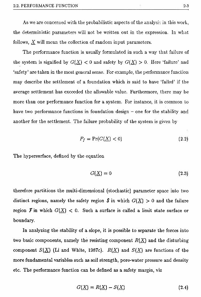
The performance function is usually formulated in such a way that failure of
the system is signified by G(X’) < 0 and safety by G(X) > 0. Here ‘failure’ and
‘safety’ are taken in the most general sense. For example, the performance function
may describe the settlement of a foundation which is said to have ‘failed’ if the
average settlement has exceeded the allowable value. Furthermore, there may be
more than one performance function for a system. For instance, it is common to
have two performance functions in foundation design - one for the stability and
another for the settlement. The failure probability of the system is given by
P; = Pr(G(X) < 0) (2.2)
The hypersurface, defined by the equation
G(X) = 0 (2.3)
therefore partitions the multi-dimensional (stochastic) parameter space into two
distinct regions, namely the safety region 5 in which G(X) > 0 and the failure
region Jin which G'(X) < 0. Such a surface is called a limit state surface or
boundary.
In analyzing the stability of a slope, it is possible to separate the forces into
two basic components, namely the resisting component R(X') and the disturbing
component S(X) (Li and White, 1987c). R(K) and .S(2Q are functions of the
more fundamental variables such as soil strength, pore-water pressure and density
etc. The performance function can be defined as a safety margin, viz
G{X) = R(X) - S(X) (2.4)
2.3. LEVEL I DESIGN 2-4
As R(2Q and S(X) are positive quantities, the performance function can also be
formulated in the following equivalent formats.
A more detailed discussion of the performance function will be given in Chapter
Fig.2.1 shows a schematic representation of Eqn.2.2. The failure probability
is given numerically by the volume bounded by the probability density function
(PDF) and the R-S plane within the failure region. For convenience, the point
(/?, 5) defined by the mean values of the distribution of R(K) and 5(X) will be
called the centroid of the distribution.
As a general rule in slope design, the further away from the limit state bound
ary the centroid is, the smaller will be the volume PQRS and hence the smaller
will be the failure probability.
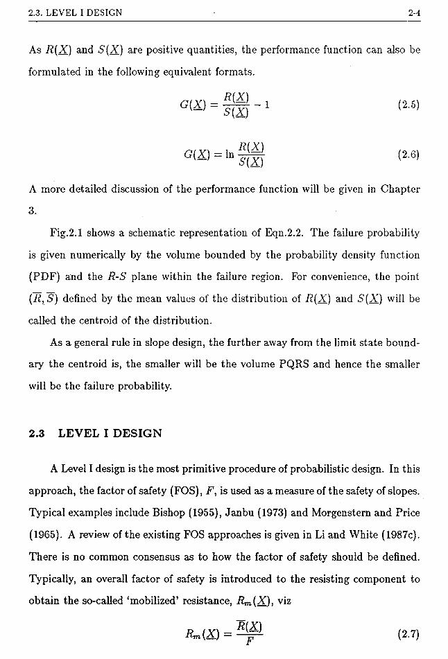
2.3 LEVEL I DESIGN
A Level I design is the most primitive procedure of probabilistic design. In this
approach, the factor of safety (FOS), F, is used as a measure of the safety of slopes.
Typical examples include Bishop (1955), Janbu (1973) and Morgenstern and Price
(1965). A review of the existing FOS approaches is given in Li and White (1987c).
There is no common consensus as to how the factor of safety should be defined.
Typically, an overall factor of safety is introduced to the resisting component to
obtain the so-called ‘mobilized’ resistance, Rm()Q, viz
(2.5)
(2.6)
3.
(2.7)

2.3. LEVEL I DESIGN 2-5
Probability density function of R J S
R > Sor G(R,S)>0Safety Region
volume = P(
R=Sor G(R,S) = 0
Limit State BoundaryR ^S
or G(R,S) <0 Failure Region
Probabilitycontours
R > S
volume = P,
R= S
( b )
Figure 2.1Joint Probability Density Function of R and S
(a) 3-D View (b) Probability Contour

2.3. LEVEL I DESIGN 2-6
The value of the factor of safety is such that the following design equation is
satisfied.
G(Rn(X),S(X))=0 or G(^p-,S(20) = 0 (2.8)
The slope is deemed to be sufficiently safe if the calculated value of F is greater
than some specified minimum value stipulated in the design code.
R
s R = S
Figure 2.2 Overall Factor of Safety Approach
The basic idea of the overall FOS approach is to ensure that the centroid of the
distribution is sufficiently far away from the limit state boundary. The specification
of a minimum value of F is equivalent to stipulating a minimum distance AC
(Fig.2.2) between the centroid and the limit state boundary. Obviously, the larger
the value of F is, the smaller will be the failure probability.

2.3. LEVEL I DESIGN 2-7
The reason that an overall FOS is only applied to the resisting component,
although not mentioned by the proponents of the FOS approach, may be justified
by the fact that the variability of the disturbing component, which is mainly due
to the weight of the soil mass, is usually less than that of the resisting component.
Therefore, the distance AC in Fig.2.2 is more important than BC in controlling
the failure probability.
AREA= A
Figure 2.3 Details of a Cohesive Slope
Although the FOS approach is simple to implement and methods are now
available whereby the value of F can be calculated very efficiently to the required
precision (Li and White, 1987a&c), it has several shortcomings which can be
discerned by the simple example of a cohesive slope as shown in Fig.2.3. The
first disadvantage of the FOS approach is the ‘variance’ of the definition of F,
that is, the value of F depends on how F is defined (Hoeg and Murarka, 1974;
Yong, 1967). With the notations given in Fig.2.3, the FOS is usually defined as
\Vldl -W2d2(2.9)

2.3. LEVEL I DESIGN 2-8
where c is the mean cohesive strength of the soil. However, some engineers prefer
to treat the soil mass W2 as contributing to the stability of the slope (particularly
if W2 includes a toe berm added for stability as indicated by the dotted lines in
Fig.2.3) and define the FOS as
cLR + W2d2W^d[
There can be a substantial difference for the computed value of F whether the
term W2d2 appears in the numerator as part of the resisting moment or in the
denominator as part of the overturning moment. The same argument applies to
the way pore-water pressure is treated in slope stability analysis. The pore-water
pressure term can appear either in the numerator or the denominator depending
on whether it is treated as a loading to the system or as a reduction to the strength
term.
Table 2.1 shows the FOS calculated using Equations 2.9 and 2.10 for some ac
tual slope designs. The difference in F is very significant in some cases. Therefore,
an ‘unsafe’ slope which has a FOS smaller than the specified value in the code may
become a ‘safe’ slope if an alternative definition is used for the calculation of F.
The second undesirable property of the FOS approach is that it is not a
consistent measure of structural safety. Table 2.2 shows the failure probability of
the slope in Fig.2.3 assuming Gaussian distributions and independence of average
shear strength and soil density. Vr and Vs in the table denote respectively the
coefficient of variation (COV) of the resisting and disturbing moment. A wide
range of values of Pj can be obtained for the same value of F. Therefore, specifying
a constant value of FOS cannot ensure a consistent risk level of slopes. As a
corollary, it is impossible to say how much safer a slope becomes as the FOS is
increased.
Fig.2.4 shows the variation of Pf with F assuming that the soil density is
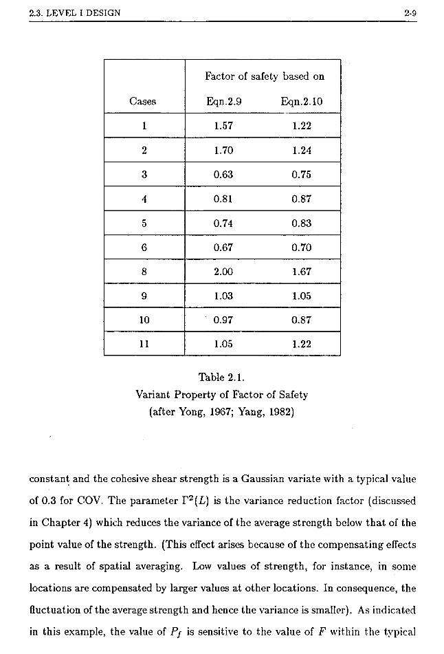
2.3. LEVEL I DESIGN 2-9
Factor of safety based on
Cases Eqn.2.9 Eqn.2.10
1 1.57 1.22
2 1.70 1.24
3 0.63 0.75
4 0.81 0.87
5 0.74 0.83
6 0.67 0.70
8 2.00 1.67
9 1.03 1.05
10 0.97 0.87
11 1.05 1.22
Table 2.1.Variant Property of Factor of Safety
(after Yong, 1967; Yang, 1982)
constant and the cohesive shear strength is a Gaussian variate with a typical value
of 0.3 for COV. The parameter T2(L) is the variance reduction factor (discussed
in Chapter 4) which reduces the variance of the average strength below that of the
point value of the strength. (This effect arises because of the compensating effects
as a result of spatial averaging. Low values of strength, for instance, in some
locations are compensated by larger values at other locations. In consequence, the
fluctuation of the average strength and hence the variance is smaller). As indicated
in this example, the value of Pj is sensitive to the value of F within the typical

2.3. LEVEL I DESIGN 2-10
Vr Vs Pf
0.2 0.2 8.3 x icr2
0.2 0.05 5.0 x 10“2
0.1 0.2 2.3 x 10~2
0.1 0.05 7.8 x 10~4
0.05 0.2 9.6 x 10“3
0.05 0.05 1.4 x 10“8
Table 2.2.Variation of Pj with Variability of Soil Property for
a Constant FOS of 1.5 (after Lumb, 1983)
range of design FOS (1.2-1.5) when the variance reduction factor is smaller than
about 0.3 which is not uncommon for real slopes.
A partial FOS approach has been proposed as an alternative to the overall
FOS approach (Hansen, 1967; Lumb, 1970 and Meyerhof, 1970&1984). A larger
FOS is assigned to the variables with greater variability and vice versa. To design
under the partial FOS approach is equivalent to checking whether the point D in
Fig.2.5 defined by (R/Fi, F2-S) where F\ and F2 are the partial factors of safety, is
in the safety domain or not. The study of the partial FOS approach is therefore to
tailor the partial FOSs in such a way that the location of D can effectively control
the failure probability to a small value. Although the partial FOS approach is an
improvement over the overall FOS approach, it cannot eliminate the shortcomings
of the FOS approach. Because of the above drawbacks, the FOS of a slope is not

2.3. LEVEL I DESIGN 2-11
1.1 1.2 13 1.4 1.5 1.6 1.7 1.8 1.9
Figure 2.4 Variation of Pj with FOS

2.4. LEVEL II DESIGN 2-12
R
Figure 2.5 Partial Factor of Safety Approach
a satisfactory risk measure.
2.4 LEVEL II DESIGN
A Level II design is also commonly known as the first-order-second moment
(FOSM) approach. In this approach, the performance function is linearized by
means of a first order Taylor’s series approximation and the random parameters
are characterized by their first two moments (hence the name).
In the following, two probabilistic approaches within the framework of a Level
II design are discussed. The first one is based on the conventional reliability index
P defined in Cornell's sense, hereafter called the /^-approach. The second one is

2.4. LEVEL II DESIGN 2-13
based on the reliability index Phl defined in Hasofer and Lind’s sense, hereafter
called the Phl-approach. Both methods will be used in Chapter 6 for analyzing
the reliability of slopes.
2.4.1 /^-approach
Because of the drawbacks of the FOS approach mentioned in the previous
section, Cornell (1969) advocated the use of the reliability index (3 as an alternative
risk format to the conventional FOS. Given a performance function G(20, the
reliability index (3 is defined as
P = llGOG
(2.11)
where hg and oq are respectively the mean and standard deviation of the per
formance function.The reason for using p as a safety measure is based on the
following observation. Defining a new variable Z by
z=c(xy-jiGCTG
the probability of failure can be written as
Pf = Pr(G(X) < 0)
_ p / G(X) ~ ^ Vg \VG <?g
= Pr(Z < -P)—0
=1- ip(z)dz
= n-fi)
(2.13)
where xp(z) and ^(2) are respectively the probability density function (PDF) and
cumulative distribution function (CDF) of Z. As a CDF is always a non-decreasing
function, a one-to-one correspondence exists between the failure probability and
2.4. LEVEL II DESIGN 2-14
the reliability index. All the uncertainties of the random variables have been
suitably condensed into the single reliability index (3. Provided that the reliability
index for two different slopes are equal, they will have a similar risk level although
the variability of the random variables may be different in the two cases. This is a
great improvement over the FOS approach as a slope with the same FOS can have
widely different risk levels depending on the variability of the input parameters.
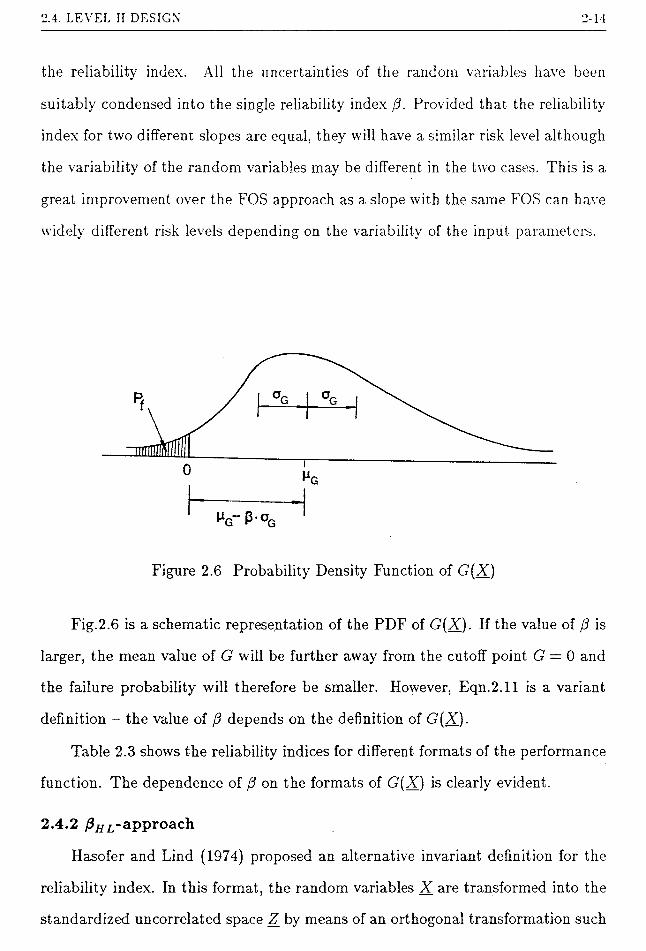
Figure 2.6 Probability Density Function of G(X)
Fig.2.6 is a schematic representation of the PDF of G(X). If the value of (3 is
larger, the mean value of G will be further away from the cutoff point G = 0 and
the failure probability will therefore be smaller. However, Eqn.2.11 is a variant
definition - the value of (3 depends on the definition of G()Q.
Table 2.3 shows the reliability indices for different formats of the performance
function. The dependence of {3 on the formats of G(X) is clearly evident.
2.4.2 /3H L-approach
Hasofer and Lind (1974) proposed an alternative invariant definition for the
reliability index. In this format, the random variables X_ are transformed into the
standardized uncorrelated space Z by means of an orthogonal transformation such

2.4. LEVEL II DESIGN 2-15
Formats 0
R-S F— 1JF’-V'+Vi
#-iF — 1
fSvr + vs
InfIn F
s/''Z + v£
Table 2.3.Formats of G'(X) and Reliability Index /? (F = /?/5)
that
= 0
i>ar{Zi} = 1 (214)
cov{Zi,Zj} = 0 i^j
Examples for transforming correlated variables into uncorrelated variables are
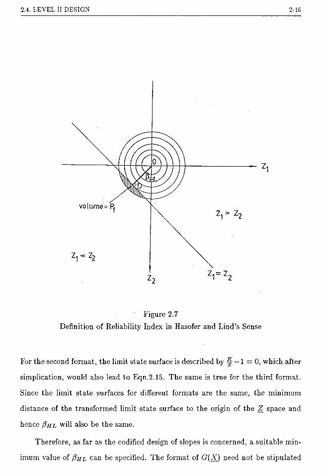
given in Ang and Tang (1984). Hasofer and Lind (1974) defined the reliability
index as the minimum distance between the origin of the Z_ space and the trans
formed limit state surface (i.e. OD in F:g.2.7). Point D is commonly called the
design point. To distinguish the reliability index defined in Hasofer and Lind’s
sense to that defined in Cornell’s sense, the former is denoted as (3hl-
The property of ‘invariance’ for /3hl is clear from its definition. As an exam
ple, let us consider the formats of G(X) given in Table 2.3. For the first format,
the limit state surface is defined by
R-S = 0 (2.15)
2.4. LEVEL II DESIGN 2-16
volume = R
Figure 2.7Definition of Reliability Index in Hasofer and Lind’s Sense
For the second format, the limit state surface is described by |r — 1 =0, which after
simplication, would also lead to Eqn.2.15. The same is true for the third format.
Since the limit state surfaces for different formats are the same, the minimum
distance of the transformed limit state surface to the origin of the Z_ space and
hence will also be the same.
Therefore, as far as the codified design of slopes is concerned, a suitable min
imum value of (3hl can be specified. The format of G'(X) need not be stipulated
2.5. LEVEL III DESIGN 2-17
as a result of the invariance of /3hl-
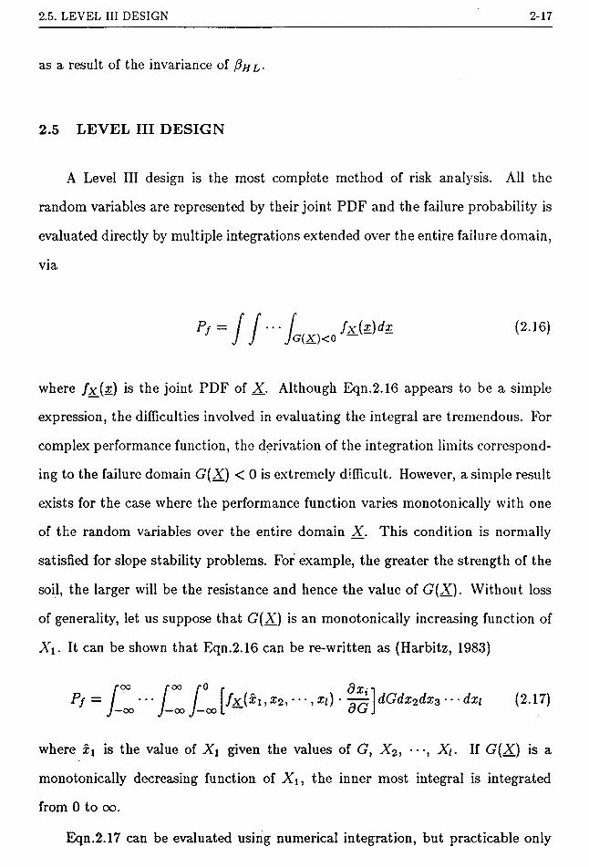
2.5 LEVEL III DESIGN
A Level III design is the most complete method of risk analysis. All the
random variables are represented by their joint PDF and the failure probability is
evaluated directly by multiple integrations extended over the entire failure domain,
via
where /x(^) is the joint PDF of X. Although Eqn.2.16 appears to be a simple
expression, the difficulties involved in evaluating the integral are tremendous. For
complex performance function, the derivation of the integration limits correspond
ing to the failure domain G'(X) < 0 is extremely difficult. However, a simple result
exists for the case where the performance function varies monotonically with one
of the random variables over the entire domain X_. This condition is normally
satisfied for slope stability problems. For example, the greater the strength of the
soil, the larger will be the resistance and hence the value of G(X). Without loss
of generality, let us suppose that G(X) is an monotonically increasing function of
X\. It can be shown that Eqn.2.16 can be re-written as (Harbitz, 1983)
where x\ is the value of X\ given the values of G, X2, •••, Xi. If G(X) is a
monotonically decreasing function of Xi, the inner most integral is integrated
from 0 to 00.
(2.16)
Pf = •'37^ dGdx^dxs ■ ■ ■ dxi (2.17)Okj .
Eqn.2.17 can be evaluated using numerical integration, but practicable only

2.5. LEVEL III DESIGN 2-18
when the dimension of X_ is small, say less than 5. Very often, repeated calculations
of Pf are necessary in an engineering analysis. A typical example is perhaps the
location of the critical slip surface of the slope. The value of Pf has to be evaluated
for each trial slip surface. In this case, the use of Eqn.2.17 will becomes very
expensive and exceedingly time consuming.
An alternative approach for evaluating Eqn.2.16 is by mean of simulation.
The Monte Carlo simulation technique is now well known and is commonly used
in reliability analysis of small problems. The accuracy of Monte Carlo simulation,
which is of order 1 /\/N where N is the number of simulations, is measured in the
statistical sense and in terms of the standard deviation of the probability estimate.
Another type of simulation which receives less attention is the number theoretic
methods (Hua and Wang, 1981). The error bound of the probability estimate ob
tained by number theoretic methods, which is of order 1/V, is absolute and can be
estimated at least in theory with the given knowledge of the performance function.
Unlike Monte Carlo simulation, the error bound for number theoretic methods de
pends on the nature of the performance function as well as the dimension of the
problem. Theoretically, the number theoretic methods are asymptotically more
efficient than Monte Carlo simulations. However, preliminary studies indicate
theoretically that number theoretic methods are preferred to Monte Carlo simula
tions only when N is exceedingly large, although a recent application by Goni and
Hadj-Hamou (1987) shows that the number theoretic methods gives more accurate
results than Monte Carlo simulation even for a relatively low value of N (of the
order of 103). Harbitz (1986) has recently proposed a procedure in which Monte
Carlo simulation is used in conjunction with the FCSM analysis to enhance the
efficiency of the simulation.
From a theoretical standpoint, a rigorous Level III design will give the most
accurate answer. In practice, a Level III method cannot be used for slope stability

2.6. APPROXIMATE LEVEL III DESIGN 2-19
analyses. This is because the joint PDF of soil properties is generally not known,
although the marginal distribution of the point property may be estimated with
some degree of certainty. Although assumptions can always be made to obtain an
answer, the value of such an analysis is lost and the tremendous effort mvolved
in the Level III calculations is not warranted. Of course, the Level III procedure
remains the only valid procedure, at least for some simple idealized cases, for
checking the validity of the Level II procedure. In the following, a number of
approximate Level III methods are discussed. These methods incorporate more
information than just the first two moments into the analysis and requires less
computation effort than a rigorous Level III analysis.
2.6 APPROXIMATE LEVEL III DESIGN
A number of approximate approaches has emerged over the past decade or
so, in attempts to provide an approximate solution to Eqn.2.16 and reduce the
computing effort of the equation. These approaches can be divided into three
main categories, namely the technique of Normal tail approximation, the method
of PDF fitting and the method of probability bound.
2.6.1 Normal tail approximation
The technique of Normal tail approximation is sometimes called the advanced-
first-order-second-moment (AFOSM) method. It can be proved (Madsen et al ,
1986) that if the performance function is linear and X follows a joint Gaussian
distribution, the reliability index Phl would be related to the failure probability
t>y
Pf = H-Phl) (2.18)
where <£(•) is the CDF of a standard Gaussian variate. If the performance function

2.6. APPROXIMATE LEVEL III DESIGN 2-20
is not highly non-linear and X_ is jointly Gaussian, Eqn.2.18 remains a good ap
proximation. Otherwise, Eqn.2.18 may give a poor answer. The basic idea of the
Normal tail approximation is to transform the non-Gaussian variates into some
kind of ‘equivalent’ Gaussian distributions so that Eqn.2.18 remains a valid ap
proximation. The mathematical formality of the Normal tail distribution is given
in Madsen et a I (1986) and Ditlevsen (1981&1983). Five different approaches of
Normal tail approximation have been proposed so far, namely Paloheimo and Han-
nus (1974), Rackwitz and Fiessler (1978), Chen and Lind (1983), Nishino et a 1 ,
(1984) and Der Kiureghian and Liu (1986).
The first four approaches are developed on the basis that the random vari
ables are independent of each other and each independent variable is represented
by means of an equivalent Gaussian distribution. For non-Gaussian dependent
variables, it is required to transform the variables into independent variables be
fore these approaches can be employed. This can be done by means of Rosenblatt’s
transformation (Rosenblatt, 1952; Hohenbichler and Rackwitz, 1981). However,
this transformation though simple in theory is very troublesome to implement
in practice and is usually highly non-linear. Although these approaches take ac
count of the non-Gaussian variables, they do not necessarily yield a better answer
using Eqn.2.18 due to the increase in non-linearity of the limit state surface. Fur
thermore, the answer is affected by the ordering of the variables taken in the
transformation (Madsen et aI , 1986).
The approach by Der Kiureghian and Liu (1986) is somewhat different to
the above four approaches. Knowing the marginal distributions and coefficient of
correlation of the variables, they devised a procedure for fitting a standard joint
Gaussian distribution to the variables. Der Kiureghian and Liu’s approach differs
from the previous methods in that the former seeks to obtain a joint PDF of X by
an equivalent joint Gaussian distribution whereas the latter aims at representing

2.6. APPROXIMATE LEVEL III DESIGN 2-21
each of the transformed independent variables by an ‘equivalent’ Gaussian dis
tribution. The approach by Dec Kiureghian and Liu for fitting a joint Gaussian
distribution appears to be simpler than Rosenblatt’s transformation required in
other approaches. If all the variables are independent, Der Kiureghian and Liu’s
approach will be the same as the method by Rackwitz and Fiessler (1978).
No comparison has yet been carried out to find out which approach of Normal
tail approximation will give the most accurate answer. Illustrative examples of
the Normal tail approximation can be found in Ang and Tang (1984) and Madsen
et a/ (1986). Further discussions and modifications of the AFOSM approach are
given in Veneziano (1974) and Fiessler et a1 (1979).
Der Kiureghian and Liu’s method has been used as one of the techniques for
slope stability analysis by Luckman (1987). Further discussion of this will be given
in Chapter 6.
2.6.2 Method of PDF fitting
The second category of approximate approaches is the method of PDF fitting.
As the name implies, the method of PDF fitting involves fitting an empirical
distribution to G(X). The failure probability is then inferred from the fitted
distribution. There are two ways by which the PDF can be fitted. The first
approach is to calculate the the statistical moments of the performance function
G(X). An empirical distribut ion is then fitted to G(X) by the Method of Moments.
Another approach involves fitting an empirical distribution using the knowledge
of the statistical moments as well as the bounds of G(X). These two approaches
will hereafter be called the approach A and approach B respectively.
2.6.2.1 Approach A
Knowing the joint PDF of X, the moments of G(X) can be calculated using
Gaussian quadratures or simulation. It should be mentioned that the simulation
technique is used herein as a numerical integration technique for calculating the

2.6. APPROXIMATE LEVEL III DESIGN 2-22
moments of G(X) whereas it is used directly for estimating the failure probability
in a rigorous Level III analysis. The moments of G(X) can usually be calculated
with a reasonable accuracy using a much smaller number of simulations than
that required for the estimation of the failure probability. The method of PDF
fitting avoids the trouble of having to find the limits of integration required for
Eqn.2.16. Furthermore, in performing the numerical integration, only the values
of G(X) at the quadrature points or the simulation points are required and the
exact functional form of G()Q does not need to be known. Therefore, the method
of PDF fitting is also applicable to implicit performance functions.
Grigoriu and Lind (1980) used the so-called optimal estimator, which is a
combination of two suitably chosen distributions, for the empirical distribution.
The parameters of the empirical distribution are obtained by matching the first
two moments of the optimal estimator and G(X). The difficulty of this method
lies in the choice of the component distributions in the formation of the optimal
estimator. The choice is very often guided by hindsight rather than foresight. The
use of this method is therefore somewhat limited. Parkinson (1978b&1983) and
Grigoriu (1983a) used the Johnson’s translation system of curves as the empirical
distribution. Grigoriu (1983b) used the lambda distributions while Li and Lumb
(1985) adopted the Pearson’s curves. Johnson’s curves, lambda distributions and
Pearson’s curves all have four parameters which can be obtained by matching the
first four moments of the theoretical and empirical distributions. The calculation
of moments of G(X) also necessitates the evaluation of n-dimensional integrals
for a set of n random variables. If n is large, the use of numerical integration is
also impracticable. For large problems, the approximate techniques developed by
Evans (1967&T972) and Cox (1979) can be used for the calculation of the moments.
2.6.2.2 Approach B
All physical quantities have bounds which may be estimated from test results

2.6. APPROXIMATE LEVEL III DESIGN 2-23
or based on the subjective judgement of an experienced engineer.
Knowing the bounds, mean value and variance of a physical quantity, it is
convenient to model the quantity by a beta distribution. The PDF of a beta
distribution has the form
ai and a2 are the lower and upper bounds of X. £q and t/2 govern the shape of
the distribution.
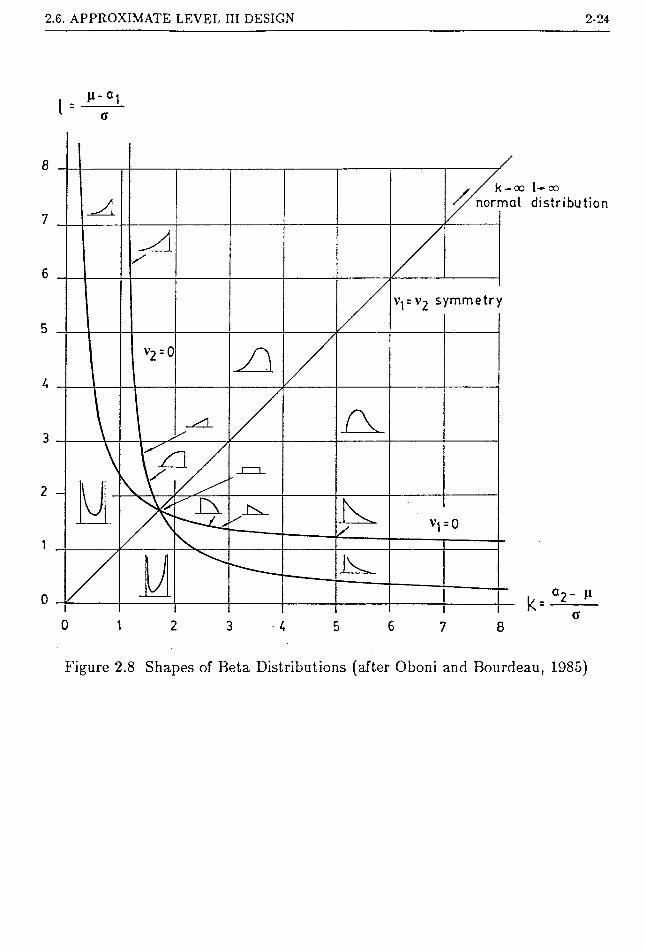
Fig.2.8 shows a wide variety of shapes covered by a beta distribution. Because
of this, a beta distribution would usually model the distribution of a bounded phys
ical quantity with a reasonable accuracy. For example, an excellent fit by a beta
distribution has been reported by Lumb (1970) for the PDF of soil strength and
by Mirza and MacGregor (1979) for the strength of steel reinforcing bars. The
estimation of the parameters of the distribution involves the first four sampling
moments (Elderton and Johnson, 1969). If the sample size is small, the sampling
variance of the third and fourth sample moments is large. A more realistic ap
proach is to establish the shape parameters *q and ia> on a larger sampling basis
for the physical quantity (for example, as reported in the literature). Assuming
that the shape parameters remain constant, the scale parameters ai and a2 can
be estimated from the sample mean value x and variance s2 using the Method of
Moments:
fx(x) <x (x - di)"1 • (a2 - x)U2 (2.19)
(2.20)
a<2 — CL\ +(iq 1^2 T 2)“ • (iq -f t'o + 3) o
[v\ 4- 1) • [v<2 -f 1)(2.21)
Alternatively, the bounds may be known for physical or engineering reasons, and
the shape parameters calculated as discussed below.
2.6. APPROXIMATE LEVEL III DESIGN 2-24
ii - a -ii = —3■1 a
/ k - oo l—00
normal distribution
Figure 2.8 Shapes of Beta Distributions (after Oboni and Bourdeau, 1985)
2.6. APPROXIMATE LEVEL III DESIGN 2-25
In this approach of PDF fitting, the bounds of the performance function are
firstly established from the knowledge of the bounds of the input parameters. This
is a problem of constrained optimization. The mean value and variance of G(Xj
can be evaluated using the FOSM method or by means of numerical integration
discussed above. Once the bounds, mean value and variance of G()Q are known,
a beta distribution can be fitted to the PDF of G(X). The failure probability
of the slope can then be inferred from the fitted distribution. The calculation of
probability for a beta variate is discussed in Harr (1977) and Kennedy and Gentle
(1980). The bounds of G(2Q would define the scale parameters a! and a2 of the
fitted distribution and the shape parameters can be obtained using
V\kl2 -21 - k
~k+lk2l -2k-l
HI
(2.22)
(2.23)
where / = (pG - «i)/crG and k = (a2 - Vg)/vg-
Obviously, the viability of the method of PDF fitting depends on the comput
ing effort required for the estimation of the bounds of G(X). The method will be
used in Chapter 6 for estimating the failure probability of slopes.
If the lower bound of G(X) is known, a Pearson’s curve can also be fitted to
G(X) by matching the lower bound and the first three statistical moments of both
distributions. The procedure is discussed in Li and Lumb (1985).
The method of PDF fitting has the advantage of simplicity and generality.
The method is reasonably accurate for well behaved distributions. The accuracy
may drop for very skewed distributions, but this is perhaps true for all approximate
methods.
2.6.2.3 Examples
Let us consider two examples of PDF fitting (Approach A) using Pearson’s
2.6. APPROXIMATE LEVEL III DESIGN 2-26
curve as the empirical distributions. For the first example, the function is G(20 =
X\ X2 — X3. The variables are taken to be independent and distributed as follows.
X\ : beta distribution
fxAx 1) a (*i “ 15)3(25 - £1)1-5
X2 : normal distribution
/i2 = 1.0 cr2 = 0.1
X3 : gamma distribution
fxAx3) « (x3 - 8) exp{—0.5(2:3 - 8)}
A Monte Carlo simulation is used to generate the empirical distribution for
(7(2Q using a total of 10,000 sets of (Xi,X2, A3). A Pearson curve is also fitted
to the PDF of G(X) by matching the first four moments. Fig.2.9 shows the
probability plot of the fitted distribution against the simulated distribution. The
fitted distribution gives excellent agreement over the range of probability level
from 0.001 to 0.999.
The second example considers the product Z of two independent standard
normal variates X\ and X2. The exact probability density function of Z is given
by (Kendall and Stuart, 1969),
fz(z) = -/STo(kl) (2.24)7T
where Ko(-) is the modified Bessel function of the second kind of zero order. The
probability integral of fz(z) is calculated from the tabulated values of the integral
of Ko(z) given in Abramowitz and Stegun (1970). Fig.2.10 shows the probability
plot for the event Pr{^ > c}. The fitted Pearson distribution gives satisfactory
approximation to the theoretical values.

TED
DISTR
IBU
TIO
N
FITT
ED
2.6. APPROXIMATE LEVEL III DESIGN 2-27
G P(g)
-10.0
SIMULATED DISTRIBUTION
(“)
G P(g)
SIMULATED D1STRIBUTIONd>)
Figure 2.9Probability Plot for Fitted and Simulated Distribution
(a) Full Range (b) Lower Portion

NO
IinaiHJLSIC
I X
3VX
J
2.6. APPROXIMATE LEVEL III DESIGN 2-28
P(z)
,~2 '
FITTED DISTRIBUTION
P(/)
Figure 2.10Probability Plot for Exact and Fitted Distribution for Z

2.6. APPROXIMATE LEVEL III DESIGN 2-29
2.6.3 Method of probability bound
The third approach is the method of probability bound. Knowing the mo
ments of G(X), it is possible to establish the upper bound of the failure proba
bility (Veneziano, 1979). The bounds are absolute, i.e. they are applicable for all
distributions having the same moments based on which the bound is established.
Unfortunately, this also means that the bound must necessarily be wide. The use
of the method is therefore limited.

CHAPTER 3
PERFORMANCE FUNCTION OF SLOPES
3.1 INTRODUCTION
There are several methods currently available for performing a slope stabil
ity analysis, viz, limit equilibrium method, limit analysis and the finite element
method.
Limit equilibrium methods consider the static equilibrium of the slip surface
in a state of incipient instability. It is perhaps the oldest numerical model for
the analysis of slope stability. The basic assumptions are (a) the failure criterion
is satisfied along the assumed slip surface and (b) the soil behaves as a perfectly
plastic material. Most of the existing limit equilibrium approaches are based on
the method of slices which was originated by Petterson in the 1910s (Petterson,
1955). The method was later extended by Janbu (1954&1973), Bishop (1955) and
Nonveiller (1965) to give the so-called generalized procedure of slices (GPS).
Limit equilibrium methods do not take account of the stress-strain relation
ship of the soil. The problem is therefore statically indeterminate. Assumptions
have to be made regarding the stress distribution within the sliding soil mass or
along the slip surface to obtain a solution. Numerous approaches to the GPS have
been proposed. They all differ in the assumptions used for the stress distribution.
Although the assumptions by these approaches vary widely, the numerical differ-
3-1

3.1. INTRODUCTION 3-2
ences of the solutions seem to be minimal (Duncan and Wright, 1980; Fredlund
and Ivrahn, 1976; Li and White, 1987c). This perhaps explains why the limit
equilibrium method can still survive this ‘modern’ age when people endeavour to
develop the most sophisticated model using, for instance, non-linear finite element
analysis.
An alternative approach called limit analysis (Chen, 1975) has also been used.
This approach derives the equations from the balance of energy at failure. How
ever, results obtained from limit analysis are essentially the same as those from the
limit equilibrium method (Chen, 1975). The approach is simple to apply for dry
homogeneous slopes and in many cases provides a closed form solution. However,
for a non-homogeneous slope with pore-water pressure, limit analysis is much more
difficult to implement than the limit equilibrium method.
With the advent of high-speed computers, the finite element method is becom
ing more and more popular in geotechnical analysis. The finite element method
is a powerful numerical tool for analyzing the stability of slopes as it can take ac
count of the stress-strain relationship of soils, follow the stress path which the soil
would experience during construction, and accomodate the changes in material
properties for different soil strata.
Though versatile it may seem, there are certain philosophical questions to
be addressed and technical problems to be solved before stochastic finite element
methods can used for probabilistic design of slopes. They are:
1. The input parameters required for finite element analysis are usually difficult
to obtain. For instance, in predicting the failure of a slope, one important
parameter is the initial stress state of the soil in the field. Except for special
projects, such information is usually not available. In the end, assumptions
which may be quite arbitrary have to be made to furnish an analysis. This
subjective uncertainty is not necessarily smaller than the model uncertainty
3.1. INTRODUCTION 3-3
associated with a simpler model such as the limit equilibrium method.
Use of the finite element method also poses a problem in the definition of the
performance function. In some analyses (e.g. Kraft and Mukhopadhyay, 1977),
the performance function is defined as a function of displacement; the problem
is then to decide which displacement (at the toe, the crown or elsewhere?) and
what displacement should constitute ‘failure’ (i.e. for the value of G(X) = 0).
The choices here are as arbitrary as choosing allowable factors of safety. In
other cases (e.g. Ishii and Suzuki, 1986), the finite element analysis may be
used to predict stresses. The performance is then defined for instance as the
safety margin of the strength values minus the stresses predicted by the finite
element method. The problem is then to establish what should be the relation
between the spatial variability of the constitutive relationship and that of the
soil strength. Clearly, there is a relationship between the two. For instance,
stiffer soils tend to have higher strength values and hence the deformation
characteristics and the strength of the soil should possess a positive cross-
correlation. In some constitutive models, such as the linear elastic model,
there is no explicit relationship between the stress-strain relationship and the
strength of the soil, thus giving us no guidelines on how the spatial variability
of these two soil properties should be modelled in statistical terms. Other
constitutive models may predict the strength values to be used. Therefore,
the statistical properties of the soil strength are established once the statistical
properties regarding the spatial variability of the parameters of the constitutive
model are specified. Of course, it is easier said than done.
A recent study by Wong (1984) shows that the total uncertainty associated with
the definition of failure, the discretization of the continuum and the choice of a
suitable constitutive model in a finite element analysis can amount to 40% to
60% of the predicted answer. In this case, one would question the credibility

3.1. INTRODUCTION 3-4
of using such a sophisticated model when it does not necessarily produce more
reliable results than simple classical methods.
Of course, there are problems such as settlement prediction which cannot be
handled by classical methods and the finite element method remains a powerful
tool for getting an answer.
2. In Chapter 4, a random field model will be introduced for modelling the stochas
tic nature of soil properties in the field. Test results do suggest that the spatial
variability of the soil parameters required in a limit equilibrium analysis (such
as strength and density) can be adequately modelled by the random field model.
To implement a stochastic finite element analysis, one has to know the spatial
variability of the constitutive relationship of the soil. Although a substantial
amount of work has been done on this subject of soil plasticity over the past
two decades or so, there are no relevant published test results regarding the
spatial variation of the parameters of constitutive models that warrant a proper
statistical analysis. Whether the random field model is suitable for modelling
the spatial variability stress-strain relationships is still unknown at this stage.
3. In a deterministic analysis, calculations only need to be performed once. In a
probabilistic analysis, the use of finite element models would usually require re
peated calculations of the performance function. For instance, using the FOSM
method, it is necessary to calculate the derivatives of the performance func
tion with respect to individual random variables. For a linear elastic analysis,
explicit expressions can be derived for the calculation of the derivatives (Ishii
and Suzuki, 1987). However, it is questionable whether a linear elastic finite
element model would produce a more accurate prediction than a limit equilib
rium analysis. For non-linear finite element analysis, the performance function
is invariably implicit. The derivatives would have to be estimated numerically,
say by finite difference approximation. As the soil properties for each element

3.1. INTRODUCTION 3-5
should be regarded as random variables, there would be at least a total ofn
1 + J2 rt calculations, where n is the number of elements and rt is the numbert=i
of random variables for each element. For n = 50 and rt = 3, which is not
atypical, a large computing effort of 151 repetitions would be required. Unless
a more efficient procedure is available, the stochastic finite element method is
likely to remain a tool of academic research.
In current approaches, the performance functions of slopes are formulated
using simple stability models such as the friction circle method (Stoyan et al, 1979;
Forster and Weber, 1981), the ordinary method of slices (e.g. Yucemen et a1, 1973;
Harr, 1977; Vanmarcke, 1980; Lee et a1, 1983; Bao and Yu, 1985; Ramachandran
and Hosking, 1985), simplified Bishop’s method (e.g. Alonso, 1976; Tobutt and
Richards, 1979; Tobutt, 1982; Anderson et al , 1982; Felio et al , 1984; Moon,
1984; Bergado and Anderson, 1985), simplified Janbu’s method (e.g. McPhail
and Fourie, 1980; Prist and Brown, 1983; Ramachandran and Hosking, 1985).
These simplified models tend to give a larger model uncertainty especially for
the ordinary method of slices and simplified Janbu’s method (e.g. Li and White,
1987c). Rigorous models have only been used very recently by Luckman (1987)
who used Spencer’s method and Li and Lumb (1987) and Li and White (1987b&e)
who adopted Morgenstern and Price’s method. A formulation based on limit
analysis was also proposed recently by Gussman (1985).
In this work, the performance function is formulated using the GPS. Different
stability models will be discussed. However, only Morgenstern and Price’s (M&P)
(1965) method will be used in subsequent analyses. M&P’s method is chosen
because it is generally regarded as one of the accurate models and is considered
to be numerically more stable than many of the existing models (Li and White,
1987c). Furthermore, some existing models can also be regarded as special cases
of M&P’s method, for instance, simplified Janbu’s method, simplified Bishop’s
3.2. BASIC EQUATIONS 3-6
method and Spencer’s method.
Conventional solution schemes for the GPS involve two levels of iteration -
one for the calculation of the interslice forces and the other for updating the FOS
(see e.g. Janbu, 1973; Fredlund and Krahn, 1976). When used in the formulation
of the performance function of slopes, such a procedure cannot give an explicit
function. As a result, the derivatives of the performance function required for a
FOSM analysis have to be calculated numerically. A new solution scheme for the
GPS is proposed herein. The new scheme has the advantage that it provides an
explicit definition of performance function without recourse to iteration for the
calculation of the interslice forces. As a result, the derivatives of the performance
function can be explicitly defined and evaluated analytically. Furthermore, the
performance function is formulated in terms of the safety margin. The advantage
of this will become clear in Chapter 6. The following presentation follows closely
to that of Li and White (1987c).
3.2 BASIC EQUATIONS
Some of the symbols and notations used in the derivation of G(X) are defined
in Fig.3.1. The subscript * denotes properties pertaining to the tth slice and the
superscript ' represents effective stress properties. The symbol ~ represents the
spatial average of a slice and the slices are numbered from 1 to n in the postive
x direction. In the derivation of the following equations, it is assumed that Ait-
is sufficiently small so that the lines of action of the vertical force and the
normal force <rt • A/t can be assumed to pass through the mid-point of the base
of the slice. Suppose that the slip surface is in a state of limiting equilibrium, the
following equations hold.

3.2. BASIC EQUATIONS 3-7
AQ: -J-
'T;Al;
AREA = A:
Figure 3.1Definitions and Notations Used in the Generalized Procedure of Slices
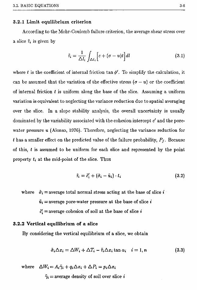
3.2. BASIC EQUATIONS 3-8
3.2.1 Limit equilibrium criterion
According to the Mohr-Coulomb failure criterion, the average shear stress over
a slice tx is given by
where t is the coefficient of internal friction tan</>'. To simplify the calculation, it
can be assumed that the variation of the effective stress (a — u) or the coefficient
of internal friction t is uniform along the base of the slice. Assuming a uniform
variation is equivalent to neglecting the variance reduction due to spatial averaging
over the slice. In a slope stability analysis, the overall uncertainty is usually
dominated by the variability associated with the cohesion intercept c! and the pore-
water pressure u (Alonso, 1976). Therefore, neglecting the variance reduction for
t has a smaller effect on the predicted value of the failure probability, Pj. Because
of this, t is assumed to be uniform for each slice and represented by the point
property tt at the mid-point of the slice. Thus
where <rt = average total normal stress acting at the base of slice i
\L{ = average pore-water pressure at the base of slice i
c[ = average cohesion of soil at the base of slice i
3.2.2 Vertical equilibrium of a slice
By considering the vertical equilibrium of a slice, we obtain
(3.1)
f, = c' + (a, - «,) • t, (3.2)
bi Ax{ = AW{ + AT{ — T{ Ax{ tan a, i = 1, n (3.3)
where AW{ — Aiii + qiAxi + A Pi = PiAxi
'ji = average density of soil over slice i
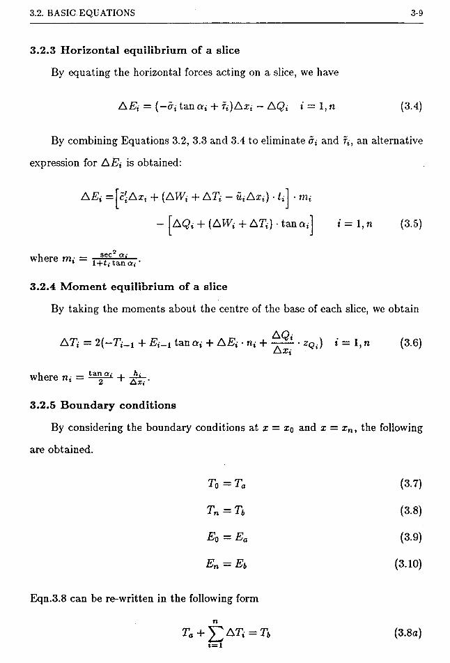
3.2. BASIC EQUATIONS 3-9
3.2.3 Horizontal equilibrium of a slice
By equating the horizontal forces acting on a slice, we have
AEt = (-at tan at + fl)Axl - AQt i = 1, n (3.4)
By combining Equations 3.2, 3.3 and 3.4 to eliminate and ft, an alternative
expression for AE{ is obtained:
A Ex = clAxl + (AWi + ATi - UiAxi) ■ tt
- ^A(?t + (AWi + ATt) • tan at i=l,n (3.5)
where m, = ■
3.2.4 Moment equilibrium of a slice
By taking the moments about the centre of the base of each slice, we obtain
AOATt = 2+ Ei-i tan at + AE{ • nt + ——- • zQi) i = 1, n (3.6)
where nt =
3.2.5 Boundary conditions
By considering the boundary conditions at x = xo and x = xn, the following
are obtained.
T0=Ta
Tn=Tb
Eq = Ea
En — Eb
E)qn.3.8 can be re-written in the following form
Ta + ytATi = Tbl=\
(3.7)
(3.8)
(3.9)
(3.10)
(3.8a)
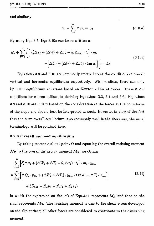
3.2. BASIC EQUATIONS 3-10
and similarly
E a + ^2 A Et = Ebi=\
(3.10a)
By using Eqn.3.5, Eqn.3.10a can be re-written as
7a + ^ j [ c'tAxt + (AWl + ATi - utAxt) • txi— i
- |AQ, + (AWi -f A Ti) • tan a, | = Eb(3.106)
Equations 3.8 and 3.10 are commonly referred to as the conditions of overall
vertical and horizontal equilibrium respectively. With n slices, there can only
by 3 x n equilibrium equations based on Newton’s Law of forces. These 3 x n
conditions have been utilized in deriving Equations 3.3, 3.4 and 3.6. Equations
3.8 and 3.10 are in fact based on the consideration of the forces at the boundaries
of the slope and should best be interpreted as such. However, in view of the fact
that the term overall equilibrium is so commonly used in the literature, the usual
terminology will be retained here.
3.2.6 Overall moment equilibrium
By taking moments about point O and equating the overall resisting moment
Mr to the overall disturbing moment Ms, we obtain
n^|c'A:rt 4- (A Wi + A Ti - utAxt) • ttt=i
n
• mt • ym.
• VQi + (AW,- + ATt) • ym. ■ tana, - AT, • x,f=( *■
(3.11)
+ (Ebyb - Eaya + Tbxb + Taxa)
in which the expression on the left of Eqn.3.11 represents Mr and that on the
right represents Ms- The resisting moment is due to the shear stress developed
on the slip surface; all other forces are considered to contribute to the disturbing
moment.
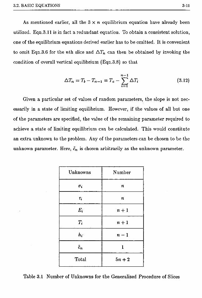
3.2. BASIC EQUATIONS 3-11
As mentioned earlier, all the 3 x n equilibrium equation have already been
utilized. Eqn.3.11 is in fact a redundant equation. To obtain a consistent solution,
one of the equilibrium equations derived earlier has to be omitted. It is convenient
to omit Eqn.3.6 for the nth slice and ATn can then be obtained by invoking the
condition of overall vertical equilibrium (Eqn.3.8) so that
n— 1ATn =rt-T„_, =Ta - Y AT, (3.12)
Given a particular set of values of random parameters, the slope is not nec
essarily in a state of limiting equilibrium. However, if the values of all but one
of the parameters are specified, the value of the remaining parameter required to
achieve a state of limiting equilibrium can be calculated. This would constitute
an extra unknown to the problem. Any of the parameters can be chosen to be the
unknown parameter. Here, cn is chosen arbitrarily as the unknown parameter.
Unknowns Number
ox n
Ti n
Ex ii -f 1
Ti n + 1
hi n — 1
Cn 1
Total 5n + 2
Table 3.1 Number of Unknowns for the Generalized Procedure of Slices

3.3. LIMIT EQUILIBRIUM MODELS 3-12
Equations Number
Failure criterion (Eqn.3.2) n
Vertical equilibrium (Eqn.3.3) n
Horizontal equilibrium (Eqn.3.4) n
Moment equilibrium (Eqn.3.6) n — 1
Overall Moment eqm. (Eqn.3.11) 1
Boundary conditions (Eqn.3.7 to 3.10) 4
Total An 4- 4
Table 3.2 Number of Equations for the Generalized Procedure of Slices
Table 3.1 summarizes all the unknowns in the GPS procedure and Table 3.2
summarizes all the equations based on limit equilibrium and boundary conditions.
The total number of unknows is 5n-f 2 while the total number of equations available
is 4n + 4. The number of unknowns therefore exceeds the number of equations by
n — 2. The analysis is therefore statically indeterminate, and n — 2 assumptions
regarding the stress acting on the slices have to made to obtain a complete solution.
3.3 LIMIT EQUILIBRIUM MODELS
As the constitutive relation of the soil is not considered in the analysis, the
problem is statically indeterminate. Assumptions have to be made to obtain an
answer. The assumptions are different for different stability models. In the fol
lowing, the equations are derived on the assumption that the slope is in a state of
limiting equilibrium. Some terminology which will be used later is defined here.
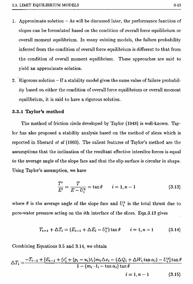
3.3. LIMIT EQUILIBRIUM MODELS 3-13
1. Approximate solution - As will be discussed later, the performance function of
slopes can be formulated based on the condition of overall force equilibrium or
overall moment equilibrium. In many existing models, the failure probability
inferred from the condition of overall force equilibrium is different to that from
the condition of overall moment equilibrium. These approaches are said to
yield an approximate solution.
2. Rigorous solution - If a stability model gives the same value of failure probabil
ity based on either the condition of overall force equilibrium or overall moment
equilibrium, it is said to have a rigorous solution.
3.3.1 Taylor’s method
The method of friction circle developed by Taylor (1948) is well-known. Tay
lor has also proposed a stability analysis based on the method of slices which is
reported in Sherard et al (1960). The salient features of Taylor’s method are the
assumptions that the inclination of the resultant effective interslice forces is equal
to the average angle of the slope face and that the slip surface is circular in shape.
Using Taylor’s assumption, we have
l7 = g - Vs = tan 0 i=l’n~1 (313)
where 0 is the average angle of the slope face and U* is the total thrust due to
pore-water pressure acting on the ith interface of the slices. Eqn.3.13 gives
Tt_! + AT{ = (£t_! + AEi - Uts) tan 0 i = l,n - 1 (3.14)
Combining Equations 3.5 and 3.14, we obtain
^ _ -Tt_! + [jEj-i 4- (c[ + (pt - ut)tj)miAxl - (AQt -f AVTt tanat) - £//] tan 61 — (mi ■ t{ — tan at) tan 9
i = 1, n — 1 (3.15)
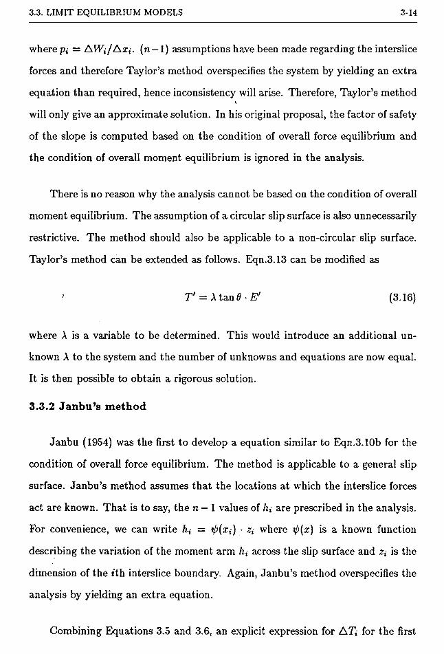
3.3. LIMIT EQUILIBRIUM MODELS 3-14
where pt = (n — 1) assumptions have been made regarding the interslice
forces and therefore Taylor’s method overspecifies the system by yielding an extra
equation than required, hence inconsistency will arise. Therefore, Taylor’s method
will only give an approximate solution. In his original proposal, the factor of safety
of the slope is computed based on the condition of overall force equilibrium and
the condition of overall moment equilibrium is ignored in the analysis.
There is no reason why the analysis cannot be based on the condition of overall
moment equilibrium. The assumption of a circular slip surface is also unnecessarily
restrictive. The method should also be applicable to a non-circular slip surface.
Taylor’s method can be extended as follows. Eqn.3.I3 can be modified as
' T' = X tan# • E' (3.16)
where A is a variable to be determined. This would introduce an additional un
known A to the system and the number of unknowns and equations are now equal.
It is then possible to obtain a rigorous solution.
3.3.2 Janbu’s method
Janbu (1954) was the first to develop a equation similar to Eqn.3.10b for the
condition of overall force equilibrium. The method is applicable to a general slip
surface. Janbu’s method assumes that the locations at which the interslice forces
act are known. That is to say, the n — 1 values of /it are prescribed in the analysis.
For convenience, we can write ht = ijj(xi) • zt where rp(x) is a known function
describing the variation of the moment arm ht across the slip surface and Z{ is the
dimension of the ith interslice boundary. Again, Janbu’s method overspecifies the
analysis by yielding an extra equation.
Combining Equations 3.5 and 3.6, an explicit expression for ATt for the first

3.3. LIMIT EQUILIBRIUM MODELS 3-15
n — 1 slices can be obtained.
A Tt = 2 • | - Xt_ i + Ei-1 tan at{
+ [ (c- + (pi ~ Ui)ti) ■ mt • Axt
1 — 2rii • (£, • — tan at)
— (AQt + Atan at) ] • nt
t = 1, n — 1 (3.17)
Janbu (1954&1973) also proposed a simplified method by taking AT; = 0.
Janbu’s method can be generalized by defining the moment arm h{ using
in which A is a multiplier. In this way, the parameter A can be adjusted to give a
rigorous solution.
3.3.3 Bishop’s method
Bishop (1955) assumed that the slip surfaces can be approximated by circles
and derived an equation similar to Eqn.3.11 for the condition of overall moment
equilibrium. Bishop (1955) did not suggest any guidelines for the calculation of the
interslice forces. However, he observed that the factor of safety based on overall
moment equilibrium is insensitive to the assumptions used for the interslice forces
and he therefore suggested the use of ATj = 0 to simplify the calculation. Such a
method is usually called the simplified Bishop method. The assumption of circular
slip surface is too restrictive and it is possible to generalize the simplified Bishop
method to non-circular slip surfaces by Eqn.3.11.
ht = Aip(xi) • (3.18)

3.3. LIMIT EQUILIBRIUM MODELS 3-16
3.3.4 Lowe and Karafiath’s method
Lowe and Karafiath’s method (1960) is similar to Taylor’s method except
that the inclination of the effective interslice forces at the interslice boundary is
assumed to be the average of the inclination of the ground surface at the top of
the interslice boundary and the inclination of the slip surface at the bottom of the
interslice boundary. Denoting the average angle by <pi, the expression of ATt for
Lowe and Karafiath’s method is given, similar to Taylor’s method, by
A Ti =-Ti-i -f [Ej-j + (c[ + (pi - Ui)ti)mjAxi - (A Qt + A Wj tan c^) - Uf] tan (pi
1 — (mi • ti — tan at) tan <pi
f = 1, n — 1 (3.19)
The same extensions as Taylor’s method can be applied to Lowe and Karafiath’s
method.
3.3.5 Morgenstern and Price’s method
M&P’s (1965) method is generally accepted as an accurate method of slope
stability because it gives a rigorous solution. The original formulation by M&P
(1965&1966) is very complex and involves the solution of two simultaneous differ
ential equations. In the following, a much simpler solution procedure is proposed.
The salient feature of M&P’s method is the assumption that the interslice
forces T{ and E{ can be related by
T{ ~ A f(xi) • Ei i = 1, n — 1 (3.20)
where A = a constant to be evaluated ;
f(x) = interslice force function.

3.3. LIMIT EQUILIBRIUM MODELS 3-17
Eqn.3.20 can be re-written as
Ti_! + ATt = Afi • (Ei-i + AEi) i = 1, n - 1 (3.21)
in which /, = /(xt). Combining Equations 3.5 and 3.21, we obtain
A Tx =— -f tan a;
t
i = 1, n — 1 (3.22)
If A is fixed, n — 1 assumptions are made and the problem will be overspecified
by yielding one redundant equation. However, if A is treated as a variable to be
determined, a rigorous solution can be obtained.
3.3.6 Spencer’s method
Spencer (1967) assumed that the inclination of resultant force of Tt and Ei is
constant, that is
where d is a value to be adjusted to give a rigorous solution. By choosing f(x) =
1 and A = tan $, Spencer’s method becomes a special case of M&P’s method.
Spencer (1973) later extended his method and suggested that T{ and Ei may be
related by
Ti—• = tan d i = 1, n — 1 (3.23)
't
Tt—f = k{ tan 0 Ei
(3.24)
where ki is a prescribed set of coefficients. Eqn.3.24 is fact identical to Eqn.3.20
if we write f(xi) = ki and A = tantf. Hence Spencer’s method is no different to
M&P’s method.
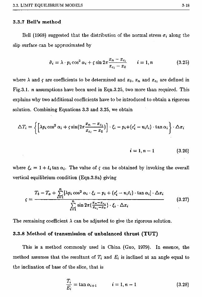
3.3. LIMIT EQUILIBRIUM MODELS 3-18
3.3.7 Bell’s method
Bell (1968) suggested that the distribution of the normal stress crt along the
slip surface can be approximated by
x — X— A • pt cos2 at + <; sin 2tt — c,
xCi - XQi = 1, n (3.25)
where A and f are coefficients to be determined and Xo, xn and xCi are defined in
Fig.3.1. n assumptions have been used in Eqn.3.25, two more than required. This
explains why two additional coefficients have to be introduced to obtain a rigorous
solution. Combining Equations 3.3 and 3.25, we obtain
A Ti = Xpi cos2 at + fsin(27r— ------—)xCi *^o .
• ft — P;+(c' — utU) • tan ai | • AX{
* = 1, n — 1 (3.26)
where = 1 -f fitanat. The value of f can be obtained by invoking the overall
vertical equilibrium condition (Eqn.3.8a) giving
nTt, — Ta + ^2 I^Pt cos2 ' ft — Pi + (c[ - Uiti) ■ tan aj] • Ax,
( = ------------- —-----n--------- —-------------------------------------- (3-27)Esm 2*(§=^).fc. Ax,
t = l '
The remaining coefficient A can be adjusted to give the rigorous solution.
3.3.8 Method of transmission of unbalanced thrust (TUT)
This is a method commonly used in China (Guo, 1979). In essence, the
method assumes that the resultant of T; and E{ is inclined at an angle equal to
the inclination of base of the slice, that is
T' f— = tan al+l i = 1, n — 1 (3.28)
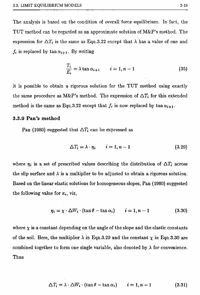
3.3. LIMIT EQUILIBRIUM MODELS 3-19
The analysis is based on the condition of overall force equilibrium. In fact, the
TUT method can be regarded as an approximate solution of M&P’s method. The
expression for AT, is the same as Eqn.3.22 except that A has a value of one and
/, is replaced by tana,+ 1. By writing
T,■rf = A tan a,+ 1 i = 1, n — 1 (35)
it is possible to obtain a rigorous solution for the TUT method using exactly
the same procedure as M&P’s method. The expression of AT, for this extended
method is the same as Eqn.3.22 except that /, is now replaced by tancq+i.
3.3.9 Pan’s method
Pan (1980) suggested that AT, can be expressed as
AT, = Xrji t = l,n—1 (3.29)
where 77, is a set of prescribed values describing the distribution of AT, across
the slip surface and A is a multiplier to be adjusted to obtain a rigorous solution.
Based on the linear elastic solutions for homogeneous slopes, Pan (1980) suggested
the following value for /c,, viz,
rji = x ’ Al• (tan 6 — tan a,) t = 1, n — 1 (3.30)
where x is a constant depending on the angle of the slope and the elastic constants
of the soil. Here, the multiplier A in Eqn.3.29 and the constant x in Eqn.3.30 are
combined together to form one single variable, also denoted by A for convenience.
Thus
AT, = A • AIT, • (tan# — tan a,) i = 1, n — 1 (3.31)

3.4. FORMULATION OF PERFORMANCE FUNCTION 3-20
It can be seen that all the expression of ATx discussed above involve only
the interslice forces on the left of each slice. With the known conditions at the
left x — x0, all the interslice forces can be calculated explicitly and successively
without the iteration required in conventional procedures.
3.4 FORMULATION OF PERFORMANCE FUNCTION
So far it has been assumed that the slope is in a state of limiting equilibrium.
To formulate the performance function, it can be argued as follows.
When the realization of the random parameters is such that the slope is in a
state of stability, the full strength would not be mobilized. Therefore, the overall
resisting moment Mr (left hand side of Eqn.3.11) based on full mobilization of
soil strength must be greater than the maximum overall disturbing moment Ms
(right hand side of Eqn.3.11) the slope can offer. On the other hand, if the slope
is in a state of instability, the maximum overall resisting moment Mr offered by
full mobilization of soil strength would not be sufficient to balance the disturbing
moment Ms acting on the slope. Therefore, the slope would be in a state of failure
or safety according as Mr < Ms or Mr > Ms. A performance function for the
slope can then be formulated as Mr — Ms. By referring to Eqn.3.11, the following
is obtained.
The subscript m signifies that the performance function is based on the condition
of overall moment equilibrium condition.
Gm(X) = ^ c[Axi 4- (AfE, + ATi - utAx,) • tx • mx • ym.t:
[AQ; • yQ{ -p (AIEt -F AT,-) • ?/m,- * AT, • xmi
- (Ebyb - Eaya +Tbxb +Taxa)(3.32)
Another performance function based on the condition overall horizontal force

3.4. FORMULATION OF PERFORMANCE FUNCTION 3-21
equilibrium can be formulated as follows. The force En can be interpreted as the
total horizontal resistance that can be offered by the slope. In a state of limiting
equilibrium, En is equal to the disturbing horizontal force Eb as indicated by
Eqn.3.10. If the slope is in fact in a stable state, the total resistance En that is
available should be greater than Eb and vise versa. Therefore, by subtracting Eb
from En and utilizing Eqn.3.10b, the following performance function is obtained.
Gf{X) =^T j [ c'iAxi + (AIT, + AT, - ^Ax,) • t-
- j^AQ* + (AWi + AT,) • tancv, | - (Eb - Ea)(3.33)
The subscript / signifies the condition of overall force equilibrium. It should be
realized that Gm(X’) and Gf()Q possess their physical meanings (Mohr-Coulomb
failure criterion and equilibrium conditions satisfied) only at the limiting condition
of G(X) = 0. At any other conditions, G(2Q only serves as an indicator function
depicting the safety-failure state of the slope.
To be correct, the moment arms xm{ and ym. should be regarded as random
variables as a result of the random forces acting on the slices. However, the
variability of xm. and ym, should be small unless AX{ is large. For practical
purpose, xmi and ymi can be treated as deterministic quantities and measured
from the centres of the bases of the slices.
An advantage of the present scheme is the explicit definition of the perfor
mance functions through the solution procedure given in previous sections. Be
cause of this, the derivatives of the performance functions Gm(}Q and Gf(2Q can
be evaluated analytically. A comprehensive list of formulae for the derivatives of
Gm(K) and G/(X) based on M&P’s method is given in Appendix A.
As will be seen later in Chapter 6, the failure probabilities inferred from
Gm(K) and Gj(X) are in general different. However, the value of A can be adjusted
so that the value of Pf derived from both performance functions are equal. The
3.4. FORMULATION OF PERFORMANCE FUNCTION 3-22
procedure of adjustment will be discussed in Chapter 6.
M&P’s method is chosen herein as the stability model for reasons given earlier.
However, other stability models based on the generalized procedure of slices can
be used in lieu of M&P’s method without much difficulty. By using the above
unified solution scheme, it is only necessary to provide one separable subroutine
for the calculation of AT; and another for evaluating the derivatives of ATt with
respect to the basic input parameters. The solution procedure for other models is
the same as that of M&P’s described in this work.
Studies indicate that all rigorous stability models give essentially the same
value of factor of safety (e.g. Duncan and Wright, 1980; Li and White, 1987d).
Although a comparison for the failure probability of slopes has not yet been done
for different stability models, it is believed that different rigorous methods will
also yield similar values of Pf.
CHAPTER 4
PROBABILISTIC MODELLING OF SOIL PROFILES
4.1 INTRODUCTION
As is commonly known, soil properties exhibit variations from point to point
even within a seemingly homogeneous soil profile. The soil properties will in
evitably fluctuate spatially and perhaps temporally in response to the changes
in the processes governing its formation such as material source, environmental
conditions and others.
Except at the sample points, the soil properties at a particular location in
the field are generally not known and therefore have to be regarded as random
variables. To properly model the stochastic nature of soil properties, infinitely
many random variables within the field have to be considered. The random field
model is now commonly used to characterize the stochastic nature of soil properties
(e.g. Vanmarcke, 1977a).
Soils generally exhibit plastic behavior although to a differing degree. As a
result, the stability of a soil slope tends to be controlled by the average soil strength
rather than the soil strength at a particular location along the slip surface. Also
the disturbing force acting on the slope is related to the average density of the soil.
The study of the statistical properties of spatial averages is therefore important
4-1

4.2. HISTORICAL DEVELOPMENT 4-2
in analyzing the stability of slopes.
This Chapter deals with the inherent variability of soils. The basics of the
random field model will be discussed and extented to cover more general types of
soil profiles. In particular, emphasis will be given to the study of the statistical
properties of spatial averages of soil properties. The relevance of sampling uncer
tainties is also discussed. This Chapter concentrates on the theory of probabilistic
modelling of soil profiles. The procedure for estimating the statistical parameters
of the random field model will be discussed later in Chapter 5. The results devel
oped here will also be used in the probabilistic analysis of soil slopes in Chapter
6.
4.2 HISTORICAL DEVELOPMENT
Unlike time series analyses, the study of spatial random processes has not been
one of the main streams of orthodox statistics. Although a spatial random process,
or random field as is called in some literature (e.g. Haining, 1977; Vanmarcke,
1984), bears some resemblance to a time series, there are importance differences
between the two. By its very nature, a time series has a time scale. There is a
natural distinction of past and future. Furthermore, the realization at a particular
instance of time depends only upon past events. Current approaches of time series
such as the autoregressive model, the moving average model and the autoregressive
moving average model are based on this fact.
A spatial random process deals with the variation of random quantities within
a spatial domain (or field). There is no such distinction of past and future and
the dependence of soil properties extends in all three directions. In consequence,
some of the classical theories of time series are not applicable to spatial processes.
Whittle (1954&1962) has done some useful work on extending the classical

4.2. HISTORICAL DEVELOPMENT 4-3
Ki.H
K. . .1-lj
K .L J
K . -
K • -bJ-1
Figure 4.1Second Order Symmetric Autoregressive Model
for a Two-dimensional Random Field
time series theory to random fields. A general discussion on the subject is also
given by Raining (1977). In describing a random field, statisticians tend to specify
the model and then generate the mean and covariance. For example, Whittle
(1954) described a discrete two dimensional field by the following second order
symmetric autoregressive model (Fig.4.1)
Kij — a(/C{+ij + Ki-ij + Ki,j+l + Ki'j— i) -f stJ (4.1)
where a is a constant and slJ is a uncorrelated random process. Generalizing
Eqn.4.1 to the continuous case yields the autocorrelation function (ACF)
p(r) = ar • Ki(ar) (4.2)
where a is a constant, r is the radial lag distance in two dimension and K\{-) is
the modified Bessel function of the second kind and order one. The calculation of

4.3. HISTORICAL DEVELOPMENT 4-4
the ACF from a given model is easier (although it is still very involved and the
procedure is discussed in Raining (1977)) than the inverse problem of finding the
model from a given ACF. Furthermore, the inverse problem does not necessarily
have an interpretable solution (Whittle, 1954; Raining, 1977).
Mining engineers and geotechnical engineers tend to specify directly the ACF
(or the variogram) without going through the procedure of model building as in
the case of Eqn.4.1. The choice of the ACF is based on convenience and also guided
by experimental results. The underlying model for the ACF is seldom of interest
to soil engineers. Provided that the assumed function is an admissible ACF and
fits well to the experimental ACF, it would be a good ACF from an engineer’s
point of view. Christakos (1984) gave some useful discussions on the criteria for a
function to be an admissible ACF.
The use of the random field theory was first introduced by Vanmarcke (1977a)
for modelling the probabilistic nature of a homogeneous soil profile. Vanmarcke
(1984) also presented the random field theory in a way that is most convenient for
application in a geotechnical reliability analysis.
In the 1960’s, a new subject called geostatistics began to take shape. The the
ory stemed from the need in the mining industry to characterize the stochastic na
ture of mineral ores. D.G. Krig is generally regarded as the creator of geostatistics,
but the mathematical formality was developed by G. Matheron and his associates
in Centre de Morphologie Mathematique, France. The standard references on the
subject are Matheron (1971), David (1977) and Journel and Huijbregts (1978).
There are many similarities between the theory of geostatistics and random
field. The major difference is that in the random field model, the correlation
structure of the spatial process is described by the autocovariance function (ACVF)
while the variogram is used in geostatistics. The ACVF and the variogram are
virtually the same, but the existence of the ACVF requires a stronger assumption

4.3. RANDOM FIELD MODEL 4-5
of second order stationarity which is not always satisfied for mineral ores. The use
of ACVF is more favoured by geotechnical engineers (e.g. Lumb, 1974<Vl975a)
partly because the concept of the ACVF is more in line with the theory of time
series and more importantly the ACVF normally exists for soil properties. For
this reason, the random field model will be used in this work, although results
established in geostatistics will also be quoted from time to time.
4.3 RANDOM FIELD MODEL
Denote the value of a soil property at a point f = (x, y, z) by /c((). In general,
K(t) can be decomposed into a trend component g(t) and a random component
e(t) with zero mean value, viz,
The trend component can be expressed as a polynomial which can be estimated
from test results at various locations tt within the field. For example,
where Pj are the terms PG = 1, Pi = x, P2 = y, P4 = z etc. For ease of reference,
the right hand side of Eqn.4.5 will hereafter be called a generalized polynomial.
While the soil properties can be measured continuously in a site investigation using,
for instance, CPT tests, there are usually physical and/or financial constraints on
the number of boreholes that can be sunk or the number of soundings that can be
k(L) = sit) + £(t) (4.3)
g(L) — ao + atx -F a2y + a3z + aAx2 + a5y2 -F aGz2 4- a7xy + etc (4.4)
For convenience, g(t) is written as
(4.5)

4.3. RANDOM FIELD MODEL 4-6
made within the field. Therefore, the trend with depth can normally be established
with a greater precision than the lateral trend component.
Except for the sample points, the realization (i.e. the actual value) of a soil
property at location < is not known and must therefore be regarded as a random
variable. The realization of a soil property at location l is in general different from
that at location V even within a so-called homogeneous soil profile. To model
the soil property correctly, one has to consider infinitely many random variables
at all locations t. This important probabilistic nature of the soil property has
not been properly recognized in much of the current literature on probabilistic
geotechnical analysis. Very often, the soil property is represented as a single
random parameter. The list for this is in slope stability analysis is overwhelmingly
long (e.g. Biernatowski, 1969,1976,1979V1987; Matsuo and Kuroda, 1974; Harr,
1977; Grivas et al, 1979; Grivas and Harr, 1979; Grivas and Nadeau, 1979; He and
Wei, 1979; Tobutt and Richards, 1979; McPhail and Fourie, 1980; Pentz, 1981;
Chowdhury, 1981; Forster and Weber, 1981; Grivas, 1981; Edil and Shultz, 1982;
McGuffey et al , 1982; Sivandran and Balasubramaniam, 1982; Tobutt, 1982;
Cheong and Subrahmanyam, 1983; Prist and Brown, 1983; Felio et al , 1984;
Moon, 1984; Nguyen and Chowdhury, 1984; Bao and Yu, 1985; Gussman, 1985;
Nguyen, 1985c; Ramachandran and Hosking, 1985; Young, 1985V1986; Wolff and
Harr, 1987). Examples in other fields of geotechnical engineering are also readily
available such as Hoeg and Murarka (1974), Ivovas and Yao (1975), Grivas (1979),
Smith (1985) and Goni and Ilaji-Hamou (1987) in retaining wall designs; Grivas
and Ilarr (1977), Madhav and Arumugam (1979), Webb (1980), Nguyen (1985a)
and Gao (1985) in foundation designs; and Krizek et al (1977), Chang and Soong
(1979), Gao (1985) and Koppula (1987) in settlement analyses; and Kuwahara and
Yamamoto (1987) in a braced excavation design.
This has the implicit implication that the soil property is perfectly correlated
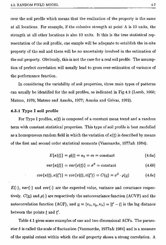
4.3. RANDOM FIELD MODEL 4-7
over the soil profile which means that the realization of the property is the same
at all locations. For example, if the cohesive strength at point A is 10 units, the
strength at all other locations is also 10 units. It this is the true statistical rep
resentation of the soil profile, one sample will be adequate to establish the in-situ
property of the soil and there will be no uncertainty involved in the estimation of
the soil property. Obviously, this is not the case for a real soil profile. The assump
tion of perfect correlation will usually lead to gross over-estimation of variance of
the performance function.
In considering the variability of soil properties, three main types of patterns
can usually be identified for the soil profiles, as indicated in Fig.4.2 (Lumb, 1966;
Matsuo, 1976; Matsuo and Asaoka, 1977; Asaoka and Grivas, 1982).
4.3.1 Type I soil profile
For Type I profiles, K,(t) is composed of a constant mean trend and a random
term with constant statistical properties. This type of soil profile is best modelled
as a homogeneous random field in which the variation of k([) is described by means
of the first and second order statistical moments (Vanmarcke, 1977aV 1984).
E{k(Q} = g(t) = a0 = m = constant (4.6a)
var{/c(/)} = var{e(t)j — o1 — constant (4.66)
cov{K(t), k(|/)} = cov{e(t_), s(i')} = C(v) = a2 • p(v) (4.6c)
E{-}, var{-} and cov{-} are the expected value, variance and covariance respec
tively. C(v) and p(-) are respectively the autocovariance function (ACVF) and the
autocorrelation function (ACF), and v = (vx,vy,vz) = \t' — 11 is the lag distance
between the points t and
Table 4.1 gives some examples of one and two dimensional ACFs. The param
eter <5 is called the scale of fluctuation (Vanmarcke, 1977a& 1984) and is a measure
of the spatial extent within which the soil property shows a strong correlation. A

4.3. RANDOM FIELD MODEL 4-8
oCl

4.3. RANDOM FIELD MODEL 4-9
O<3
cdrd(X<vmItc
.2'53CO£
o£
GcdGJGo
-225
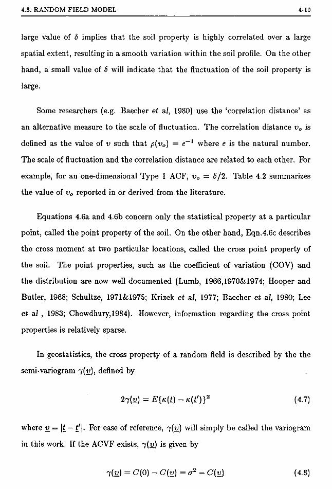
4.3. RANDOM FIELD MODEL 4-10
large value of <5 implies that the soil property is highly correlated over a large
spatial extent, resulting in a smooth variation within the soil profile. On the other
hand, a small value of 8 will indicate that the fluctuation of the soil property is
large.
Some researchers (e.g. Baecher et a/, 1980) use the ‘correlation distance’ as
an alternative measure to the scale of fluctuation. The correlation distance vQ is
defined as the value of v such that p(va) = e~l where e is the natural number.
The scale of fluctuation and the correlation distance are related to each other. For
example, for an one-dimensional Type 1 ACF, vQ = 8/2. Table 4.2 summarizes
the value of vQ reported in or derived from the literature.
Equations 4.6a and 4.6b concern only the statistical property at a particular
point, called the point property of the soil. On the other hand, Eqn.4.6c describes
the cross moment at two particular locations, called the cross point property of
the soil. The point properties, such as the coefficient of variation (COV) and
the distribution are now well documented (Lumb, 1966,1970&;1974; Hooper and
Butler, 1968; Schultze, 1971&1975; Krizek et a/, 1977; Baecher et a/, 1980; Lee
et a/ , 1983; Chowdhury,1984). However, information regarding the cross point
properties is relatively sparse.
In geostatistics, the cross property of a random field is described by the the
semi-variogram 7(4;), defined by
27(v) = E{k(Q - K(t')}2 (4.7)
where v = \t — t'\. For ease of reference, i(v) will simply be called the variogram
in this work. If the ACVF exists, 7(2;) is given by
7(v) = £7(0) - C(v) =o2- C(v) (4.8)
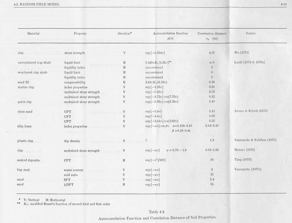
4.3. RANDOM FIELD MODEL 4-11
Material Property direction* Autocorrelation function
P{v)Correlation distance
v0 (m)Source
clay shear strength V exp{-0.234u} 4.27 Wu (1974)
unweathered cl ly shale liquid limit H 0.445vA'i (1.31v)** « 0 Lumb (1974 & 1975a)liquidity index H uncorrelated 0
weathered clay shale liquid limit H uncorrelated 0liquidity index H uncorrel ated 0
sand fill compressibility H 3.81u/\ i(6.25u) 0.16marine clay index properties V exp{-1.23u} 0.81
undrained shear strength V exp{-0.33u} 3.03undrained shear strength V exp{-3.75u} cos(7.73u) 0.12
quick clay undrained shear strength V exp{— 0.35u} cos(6.28v) 0.19
clean sand CPT V exp{-0.9u} 1.11 Alonso & Krizek (1975)
CPT V exp{-1.6v} 0.63
CPT V exp{ —1.91u} cos(2.62u) 0.32
silty loam index properties V exp{— an} cos fiv a=0.158-3.10 2.14-3.10p =0.23-0.41
plastic clay dry density V ? 1.3 Vanmarcke & Fuleihan (1975)
clay undrained shear strength V exp{-au} a = 0.75 — 1.6 0.63-1.33 Matsuo (1976)
seabed deposits CPT H exp{-v2/900} 30 Tang (1979)
bay mud water content V exp{-au} 9 Vanmarcke (1977c)
void ratio V exp{-au} 10sand SPT V exp{—au} 2.4sand 1/SPT H exp{-au} 55
* V: Vertical H: Horizontal** K\: modified Bessel’s function of second kind and first order
Table 4.2.Autocorrelation Function and Correlation Distance of Soil Properties

4.3. RANDOM FIELD MODEL4-12
Material Property direction* Autocorrelation function
p{v)
Correlation distance
v0 (m)
Source
coastal sand CPT ? ? 5 Baecher et a/ (1980)compacted clay dry density V ? 1.2compacted clay dry density II ? 5compacted clay dry density V ? 5dune sand SPT ? ? 20
sand hydralic conductivity H&V ? < lm Smith (1981)sand porosity H&V ? < lmsand Do o H&V ? < lm
sand In Dr H exp{-v/34} 34 Fardis &: Veneziano (1981)sand In Dr H exp{-u/1.8} 1.8
soft clay undrained shear strength V exp{—vj\.2\] 1.21 Asaoka Grivas (1982)soft clay undrained shear strength V exp{-u/3.11} 3.11
alluival deposit l/CPT V exp{-au} a = 0.78 - 23.13 0.4 -1.3 Ximenez de Embun & Romana (1983)
soft glacial clay undrained shear strength V ? ~lm Wu & El-Jandali (1985)
soft glacial clay undrained shear strength V ? ~lm
silty seabed sand CPT V ? ~lm
silty clay CPT V exp{-u/0.1} 0.1m Author’s data
Table 4.2. (cont.)

4.4. STATISTICS OF SPATIAL AVERAGES 4-13
Since C(v) normally approaches zero for a large distance, 7(2;) will approach the
point variance a2 of the soil property as v increases.
4.3.2 Type II soil profile
In a Type II soil profile, ic(t_) can be decomposed into a non-constant trend
component and a random component with constant statistical properties. The
random component can be modelled in the same way as a Type I soil profile.
II
'-w (4.9a)
var{K,(t)} — var{e(i)} — o2 — constant (4.96)
/c(f), /c(f')} = cov{e(l),£(i')} = a2 • p(v) (4.9c)
Typically, g(t) will be estimated as a linear function.
4.3.3 Type III soil profile
In this type of soil profile, the random component of the soil property possesses
a constant coefficient of variation. However, e(t) can be transformed into another
random component r/(f) with zero mean value and constant variance, a2, via,
e(L) = g(L) ■ v(L) (4.10)
The transformed random component 77 (^) can also be modelled as a homogeneous
random field (Asaoka and Grivas, 1982). Thus
E{k(Q} = g(t) (4.11a)
var{K,(t)} = var{e(t)} = g2(t) • a2 (4.116)
cov{K(t),K(t_')} = cov{e(t),e(t')} = g(t) • g{t_') • a2 • p(y) (4.11c)

4.4. STATISTICS OF SPATIAL AVERAGES 4-14
4.4 STATISTICS OF SPATIAL AVERAGES
The performance of geotechnical structures is usually governed by average
soil properties. In slope stability analysis, the average soil properties such as the
spatially averaged cohesion or soil density are of interest rather the point properties
of the soil. The spatial average of a soil property *c(£) is defined as
where V can be the length L, area A or volume V of the spatial domain depend
ing on the case and gy and ey are respectively the spatial average of the trend
component and the random component. In a slope stability analysis, the domain
V would typically be the base or the area of a slice. The mean value, variance and
covariance of the spatial averages are given by
(4.12)
(4.13)
var{/c\/} — Eygy + iy —
= E{gy + Sy — gy}2(4.14)
— E{iy}2
= var{ey}
— E{iy • £yi}
= COv{iy,6y>}
(4.15)

4.4. STATISTICS OF SPATIAL AVERAGES 4-15
4.4.1 Type I and II soil profiles
For Type I and II soil profiles, Eqn.4.14 can be written as
var{ky} = var{ev)
= ^e{ [ 6(t)dt j2
= ^ ett'm' 1
= T / / £{£(<)£(<')}<M'
= hjvjv p(-)dLdt-= <t2- r2(K)
(4.16)
where r2(E) = ^ fv fv p{v)dtdi' is called herein the variance reduction factor.
For the covariance, we have
where B(V, V') = ^77 Jy// JV p{v)dtdt'. B(-) is called herein the covariance factor.
To implement the two dimensional stability analysis using Morgenstern and
Price’s method in Chapter 6, it is necessary to know the variance reduction and
covariance factors for spatial averages over the bases of the slices and the area of
the slices. The variance reduction and covariance factors can always be evaluated
using numerical integration. However, owing to the fact that the lag distance does
not vary smoothly with the location variables t, a quadrature with a relatively
COv{kv,ky>} = COv{iy, Sy)
(4.17)
= <t2 ■ B(V,V')

4.4. STATISTICS OF SPATIAL AVERAGES 4-16
large number of integration points is required to achieve a reasonable accuracy.
This will incur a heavy time penalty in generating the covariance matrix of the
spatially averaged soil properties. Here, a procedure will be outlined by which the
variance reduction and covariance factors can be evaluated semi-analytically and
more efficiently.
4.4.1.1 Variance reduction factor for line averages
Referring to Fig.4.3, the variance reduction factor for a line average is given
by
r2(L) = T fL [L P(Vl,vy)didi' (4.18)
where vx = \l' — /|cos# and vy = |/' — /|sin0. By introducing the change of
variables (tx = /, 72 = — /), the domain of integration will be changed as indicated
in Fig.4.3. By carrying out the integration with respect to Ti, Eqn.4.18 becomes
p(|r2|cos0, |72|sin0)d7i dr2+
p(\r2\cos0, |72| sin 9)dTldT2
Z2 (L- 72)/?(|72|cos0, |r2|sin0)dr2+
fo/ ^(L + t2)p(\t2\cos 6, \t2\sm 0)dr2 (4.19)
Note that the first integral is evaluated over the domain Si in Fig.4.3 where
72 is always postive and hence the absolute sign can be removed from the first
integral. On the other hand, the second integral is evaluated over the domain S2
where 72 is always negative. However, by introducing a further transformation
r2 = —72, the domain of integration for the second integral can now be converted
to B2 within which r2 is always positive and therefore the absolute sign can also
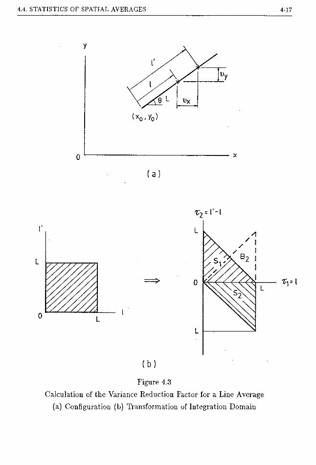
4.4. STATISTICS OF SPATIAL AVERAGES 4-17
x2-
(b)
Figure 4.3Calculation of the Variance Reduction Factor for a Line Average
(a) Configuration (b) Transformation of Integration Domain

4.4. STATISTICS OF SPATIAL AVERAGES 4-18
be removed. After simplification, Eqn.4.19 becomes
(4.20)
Once the ACF is given, Eqn.4.20 can be integrated directly to give the variance
reduction factor. Alternatively, numerical integration can be used. As Eqn.4.16
involves only a single integral and the arguments of p(-) now vary smoothly with
the integration parameter, a low order numerical quadrature will be sufficient to
give a reasonable accuracy. The variance reduction factors for the separable two
dimensional ACFs listed in Table 4.1 are given in Table C.l in Appendix C.
r2( l)1.0
0.5
0.00 5
l6
10 15 20
Figure 4.4
Variance Reduction Factor for Line Average - Type I ACF
The variance reduction factor is bounded by 0 and 1. Therefore, the variance
of the spatial average is smaller than that of the point property. Fig.4.4 shows the

4.4. STATISTICS OF SPATIAL AVERAGES 4-19
general trend for T2(-) for a one-dimensional Type I ACF. The pattern is similar
for two or three dimensional cases. The figure indicates that T2(•) diminishes as
the ratio L/8 increases. For line averages, it can be proved for Svell-behaved’
ACFs (i.e. it decays sufficiently fast as v increases) that the variance reduction
factor can be approximated for a large averaging length by (Vanmarcke, 1984)
The approximation is good when L > 28. Similar expressions can also be estab
lished for two and three dimensional spatial averages (Vanmarcke, 1984).
For some natural soils, the correlation distance of soil properties is small, of the
order of l-2m (see Table 4.2). The reduction of variance due to spatial averaging
can therefore be appreciable without the averaging dimension being very large.
This has a very important implication. Although it may be very discomforting to
realize that a coefficient of variation of greater than 40% (point property) is not
uncommon for the undrained shear strength of soil (Alonso, 1976), the variability
of the average shear strength, which governs the performance of slopes, is usually
much less than the point variability.
4.4.1.2 Covariance factor for line averages
Referring to Fig.4.5 and using Eqn.4.17, the covariance factor of two line
averages is given by
where vx = \vxo + l' cos 02 — l cos 9\| and vy = \vyo + l' sin 02 — / sin 9\|. Two cases
have to be considered.
(4.21)
(4.22)
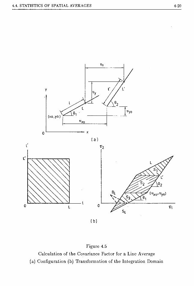
4.4. STATISTICS OF SPATIAL AVERAGES 4-20
(xo,yo)
Figure 4.5Calculation of the Covariance Factor for a Line Average
(a) Configuration (b) Transformation of the Integration Domain

4.4. STATISTICS OF SPATIAL AVERAGES 4-21
1. Case 1 — 61 7^ 02
By making the transformation
74 = yxo + l' cos Qq, ~ l cos 61
(4.23)r2 = vyo + l' sin 02 — / sin 9i
Eqn.4.22 will be transformed into
J JsP(\n\,\T2\)dTidT2 (4.24)
where t] is the Jacobian determinant and S is the domain of integration in the
7i~t2 space. An example of the transformed domain is given in Fig.4.5. To
perform the integration, the region S can be divided into suitable subregions.
If Ti and r2 are positive within the subregion, the absolute sign can be removed.
If tj or r2 is negative, an additional transformation of 74 = —T\ or r2 = —r2
or both is necessary to change the subregion into one in which T\ and r2 are
positive so that the absolute sign can be removed. An example in given in
Fig.4.5. To is negative in subregion S4. By transformation r2 = —r2, the domain
of integration is now transformed to B4 in which r2 is positive. Following the
above procedure and integrating first with respect to 74, Eqn.4.24 can be re
written as
all subregions. The Jacobian determinant r/ and the constants of the integral I
are given in Table C.2 for some basic configurations of lines L and L' that will
be encountered in the analysis of a general non-circular slip surface. Formulae
for calculating he integral It for the two dimensional ACFs given in Table 4.1
(4.25)
where /, = j£‘ P(T 1 > T2)dTt dr2 and the summation in Eqn.4.25 is over
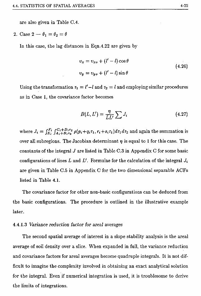
4.4. STATISTICS OF SPATIAL AVERAGES 4-22
are also given in Table C.4.
2. Case 2 — 6\ — 02 — 0
In this case, the lag distances in Eqn.4.22 are given by
vx = vxo + (/' - /) cos 6
vy = vyo + (/' - /) sin0(4.26)
Using the transformation Ti = /'—/ and r2 = l and employing similar procedures
as in Case 1, the covariance factor becomes
over all subregions. The Jacobian determinant r] is equal to 1 for this case. The
constants of the integral J are listed in Table C.3 in Appendix C for some basic
configurations of lines L and L'. Formulae for the calculation of the integral Jt
are given in Table C.5 in Appendix C for the two dimensional separable ACFs
listed in Table 4.1.
The covariance factor for other non-basic configurations can be deduced from
the basic configurations. The procedure is outlined in the illustrative example
later.
4.4.1.3 Variance reduction factor for areal averages
The second spatial average of interest in a slope stability analysis is the areal
average of soil density over a slice. When expanded in full, the variance reduction
and covariance factors for areal averages become quadruple integrals. It is not dif
ficult to imagine the complexity involved in obtaining an exact analytical solution
for the integral. Even if numerical integration is used, it is troublesome to derive
the limits of integrations.
(4.27)
where J{ = f£'{ Ja^+b-t^ /9(Pi+<7i7’i, rl+str1)dr1dr2 and again the summation is
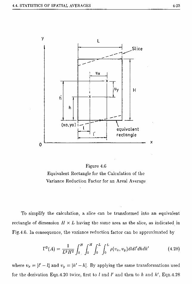
4.4. STATISTICS OF SPATIAL AVERAGES 4-23
Slice
l)X
H
K<
Uy
h
(xo,yo)-1"
r
\equivalent
rectangle
Figure 4.6Equivalent Rectangle for the Calculation of the Variance Reduction Factor for an Areal Average
To simplify the calculation, a slice can be transformed into an equivalent
rectangle of dimension H x L having the same area as the slice, as indicated in
Fig.4.6. In consequence, the variance reduction factor can be approximated by
r2(^4) = 22772 // J" jQL J0L /»(*>*. vy)dldl'dhdh' (4.28)
where vx = \l' — /| and vy = \h' — h |. By applying the same transformations used
for the derivation Eqn.4.20 twice, first to / and l' and then to h and /i', Eqn.4.28

4.4. STATISTICS OF SPATIAL AVERAGES 4-24
can be reduced to the following double integral.
r2M) = JYJp J0 L -T2)p(TuT2)dTldT2 (4.29)
If the ACF is separable, it can be written as /9(r1,r2) — Pi Eqn.4.29
then becomes
r2(A = r2(L) -r2(H) (4.30)
Eqn.4.30 is simply the product of the variance reduction factors of the line averages
over the sides of the rectangle. The reduction in computing effort for this case is
very large.
4.4.1.4 Covariance factor of areal averages
The equivalent rectangle approximation can also be used for the covariance
factor. In this case, the covariance factor is given by (Fig.4.7)
1 r H/ r H r L* r LB(A, A') = 77777777 / / / / p(vx,vy)dldl'dhdti (4.31)
LL'nrT Jo Jo Jo Jo
where vx = |/' — /| and vy = \h' — h|.
Two basic configurations as shown in Fig.4.8 are of interest. For the configu
ration in Fig.4.8a, the covariance factor is given as (Vanmarcke, 1984)
b(a’ a']=£(_i)t ■ <l* x h]2 ■ r2(-4,) (4-32)
where r2(At) is the variance reduction factor for a rectangle of dimension H x L*.
The covariance factor for the second basic configuration (Fig.4.8b) is (Vanmarcke,
1984)
B(A, = D->)‘+y • W x A*)2 • r2(^>) (4-33)t=0j—0
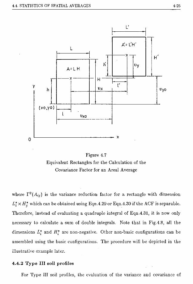
4.4. STATISTICS OF SPATIAL AVERAGES 4-25
A= L H
Figure 4.7
Equivalent Rectangles for the Calculation of the
Covariance Factor for an Areal Average
where T2(AlJ) is the variance reduction factor for a rectangle with dimension
L* x H* which can be obtained using Eqn.4.29 or Eqn.4.30 if the ACF is separable.
Therefore, instead of evaluating a quadruple integral of Eqn.4.31, it is now only
necessary to calculate a sum of double integrals. Note that in Fig.4.8, all the
dimensions L* and H* are non-negative. Other non-basic configurations can be
assembled using the basic configurations. The procedure will be depicted in the
illustrative example later.
4.4.2 Type III soil profiles
For Type III soil profiles, the evaluation of the variance and covariance of
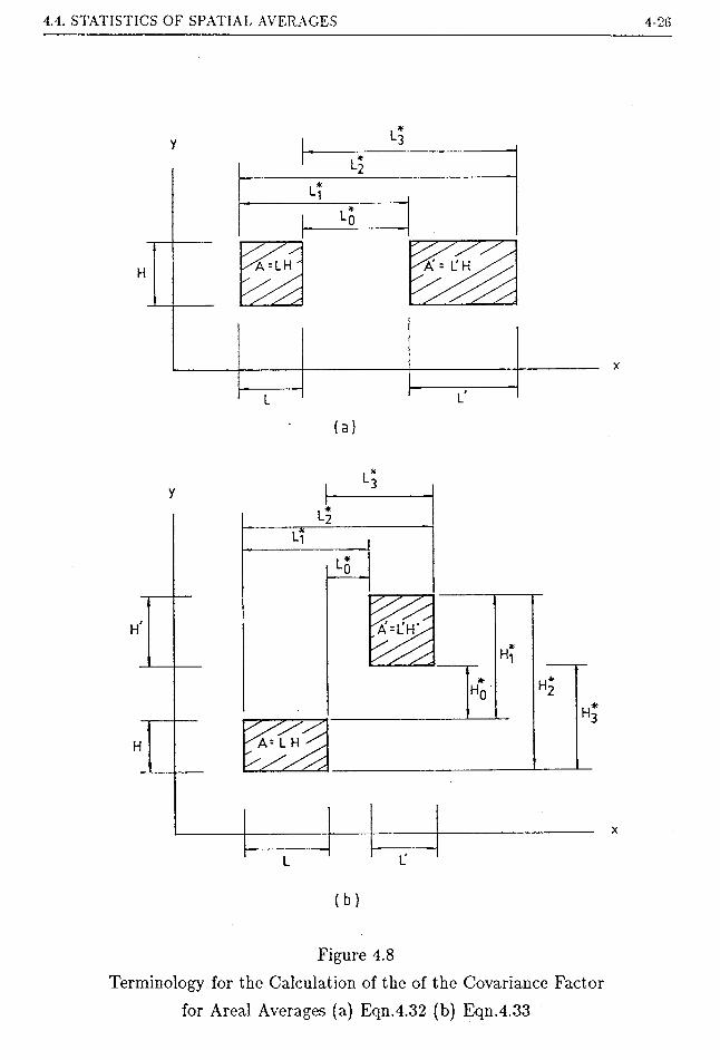
4.4. STATISTICS OF SPATIAL AVERAGES 4-26
A - L' H"A =LH '
a=l'h;
L L'
(b)
Figure 4.8
Terminology for the Calculation of the of the Covariance Factor
for Areal Averages (a) Eqn.4.32 (b) Eqn.4.33

4.4. STATISTICS OF SPATIAL AVERAGES 4-27
spatial averages is more complicated. They are described by
2var{ev} = ^ g(t)g(t')p(v)dtdt! = o2 • E2(V) (4.34)
cov{ev,Ev} = g(L)g{t_')p(v)dt_dt_' = a2 • D(V, V') (4.35)
where E2(-) and D(-) are also called the variance reduction and covariance fac
tors for convenience despite the fact that they are defined differently to T2(K)
and B(V,V). Denoting the two dimensional trend component g(t;) by g(x,y) and
following a similar procedure as in Equations 4.19 and 4.20 for the calculation of
T2(L), the variance variance factor of a line average for Type III soil profiles is
given by (Fig.4.3)
1 rL rLE 2(L) = — I g(x0 + l cos0,yo + ls\n9) ■ g(x0 + l'cos9,y0 + l's\n9)-1 fL CL
L* „
p(\l' — /| cos#, \l' — l\ sin 6)dldl'■ rL rL—r21
LrL, rL-r2
I g[x0 4- Ti cos9, yQ + Ti sm 9)-
g(x0 + (n + T2) cos0, y0 + (ti + r2) sin0)-
p(\r2\cos9, \t2\s\n9)dTldT2 +
J lJ 9(xo + Ticos0,y° + TisinO)-
g(x0 + {Ti + T2)cos6,y0 + (ri + 72)sin0)-
p(\t2\cos 9, \t2\ sin 9)dTidr2
i rLl= j2 L ^(r2 c°s0, t2 sin 9)
\lL—t2
g(xQ + ri cos 9, yQ + Ti sin 9)-
g(xQ -f (rx + t2) cos9, yQ + (ti + t2) sin 0)dTx +
g(xc + Ti cos9, yQ + Ti sin ^)*
g(xQ + (t - 72) cos 9, y0 + (ti - T2)s\n9)dTi dr2
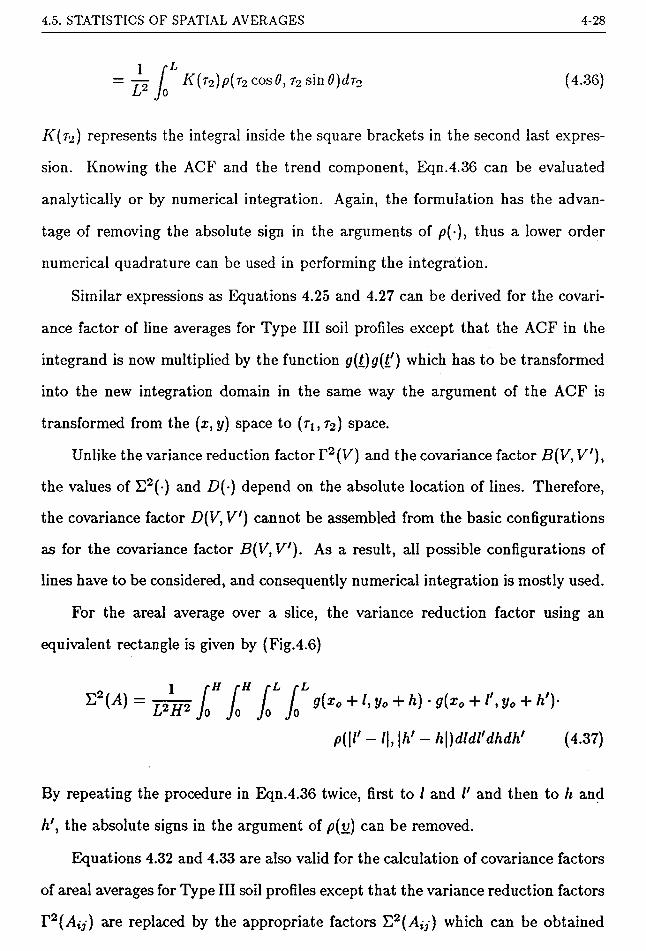
4.5. STATISTICS OF SPATIAL AVERAGES 4-28
LK(tz)p(t2 cosO, ro sin 0)(It2 (4.36)
K(t2) represents the integral inside the square brackets in the second last expres
sion. Knowing the ACF and the trend component, Eqn.4.36 can be evaluated
analytically or by numerical integration. Again, the formulation has the advan
tage of removing the absolute sign in the arguments of /?(•), thus a lower order
numerical quadrature can be used in performing the integration.
Similar expressions as Equations 4.25 and 4.27 can be derived for the covari
ance factor of line averages for Type III soil profiles except that the ACF in the
integrand is now multiplied by the function g(t)g(t') which has to be transformed
into the new integration domain in the same way the argument of the ACF is
transformed from the (x, y) space to (ri, To) space.
Unlike the variance reduction factor r2(Vr) and the covariance factor B(V, V'),
the values of E2() and D(-) depend on the absolute location of lines. Therefore,
the covariance factor D(V, V') cannot be assembled from the basic configurations
as for the covariance factor B(V, V'). As a result, all possible configurations of
lines have to be considered, and consequently numerical integration is mostly used.
For the areal average over a slice, the variance reduction factor using an
equivalent rectangle is given by (Fig.4.6)
~ IJfP L Jo Jo Jo + /, I/o -+- /i) - -f- A')-
p(\l‘ - /|, |A' - h\)dldl'dhdti (4.37)
By repeating the procedure in Eqn.4.36 twice, first to l and /' and then to h and
h', the absolute signs in the argument of p(v) can be removed.
Equations 4.32 and 4.33 are also valid for the calculation of covariance factors
of areal averages for Type III soil profiles except that the variance reduction factors
r2(Aty) are replaced by the appropriate factors E2(Aty) which can be obtained

4.5. WHITE NOISE PROCESS 4-29
using Eqn.4.37.
4.5 WHITE NOISE PROCESS
As the scale of fluctuation 6 approaches zero, the random field will degenerate
into an uncorrelated random process and T2(-) and £2(-) will also approach zero.
It might be thought that the variance of the spatial average would also approach
zero as b tends to zero, but this is not the case. The associated point variance of a
white noise process must go to infinity (see e.g. Priestley, 1981), but the products
cr2 - r2(Vr) and <r2 • £2(P) remain finite.
The ACVF of a white noise process can be represented as a Dirac ^-function.
C(v) =u = 0
(4.38)
Given a continuous function f(t), for a point € V and v = L0~L we have
Jvf(L)C(v)dL = f(t0)-w (4.39)
where w is called the white noise intensity with the dimension of variance x V.
For Type I and II soil profiles, the variance of a spatial average is given by
var{ky} = ^ J j C(v)didt'
= ±Jv wdt_' (4.40)
w = V
The covariance of two spatial averages in two non-overlapping domains is given by
cov{£v, k'V'} W> JvfvCMW (4.41)

4.6. COMPOSITE RANDOM PROCESS 4-30
where t G V, t' G V and v_ — \i — L'\- As v is always greater than zero, C(v)
will become zero. Consequently, cov{ky, ky>} — 0 for non-overlapping spatial
averages.
For Type III soil profiles,
Similarly, it can be proved that cov{ky, k y} = 0 for two non-overlapping regions.
4.6 COMPOSITE RANDOM PROCESS
The ACFs listed in Table 4.1 are all ‘simple’ functions, in the sense that
they decay from 1 at zero lag to zero at large lag distances in a smooth and
uninterrupted manner. Furthermore, the ACF is governed by a single parameter
which can be directly related to the scale of fluctuation.
For more complex random processes, the random component e(<) can be rep
resented as a sum of statistically independent random components
(4.42)
e(L) — e\ {Q + £2(0 + • • • + £k{L) (4.43)
each with a different scale of fluctuation. For example, S\ (t) may represent the
nugget effect (see later) and €2(1) a strongly correlated random component etc. A
number of simple results follow from this model. For example

4.7. NUGGET EFFECT 4-31
kC(t>) =
tTTi(4.45)
kvar{iy} = var{iy^}
t=i(4.46)
kcov{ev, ev>) = y cov{Ey\ey}} (4.47)
i = l
where the subscript and superscript i represent quantities related to £,(/). The
above composite random process (or nested structure as known in some literature)
is widely used in geostatistics (e.g. David, 1977; Journel and Iluijbregts, 1978) to
approximate a random field with complex correlation structure.
4.7 NUGGET EFFECT
Sometimes, a discontinuity is found to occur in the sample autocovariance
function and autocorrelation function at zero lag.
An example of this is shown in Fig.4.9. Other examples can be found in Lumb
(1975a), Baecher (1984) and VVu and El-Jandali (1985) and are also commonly
found in books on mining geostatistics such as Agterberg (1974), David (1977),
Journel and Huijbregts (1978) and Clark (1979). In mining geostatistics, such a
phenomenon is called a nugget effect. There are three possibilities which give rise
to the occurrence of the nugget effect.
1. The sampling interval is large compared with the scale of fluctuation so that
the details of the ACVF at small lag distances can not be reviewed.
2. The soil property possesses a random component which has a very small value
of 6 and behaves like a white noise process. For ease of reference, this kind of
process is called a small-<5 process.
3. The presence of measurement errors also gives rise to the nugget effect. Using
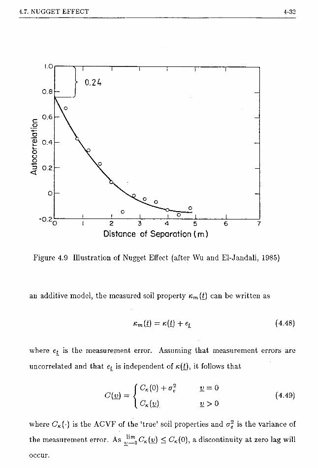
Aut
ocor
rela
tio
4.7. NUGGET EFFECT 4-32
Distance of Separation (m)
Figure 4.9 Illustration of Nugget Effect (after Wu and El-Jandali, 1985)
an additive model, the measured soil property Km(t) can be written as
Km(t) = K(t) + et_ (4.48)
where e*_ is the measurement error. Assuming that measurement errors are
uncorrelated and that is independent of ac(/), it follows that
C(v) =CK(0) + &e
CK(V)
v — 0
v>0(4.49)
where C'K(-) is the ACVF of the ‘true’ soil properties and is the variance of
the measurement error. As CK (v) < CK(0), a discontinuity at zero lag will
occur.

4.7. NUGGET EFFECT 4-33
If the nugget effect is due to the first cause, the question arises of how small
should be the sampling interval so that sufficient details of the ACF at small lag
distances can be reviewed. The following concept is useful. In a slope stability
design, preliminary investigations can be carried out to establish the variation of
the failure probability with the scale of fluctuation based on some prior knowledge
of the variability of soil properties. Suppose it is established for a particular design
that a scale of fluctuation less than 3m will correspond to a sufficiently low value
of failure probability.
With this in mind, a sampling interval equal to, for instance, 1/10 of this
value, i.e. 0.3m, can be used. If the scale of fluctuation is indeed greater than
3m, the design will not be acceptable. However, a sampling interval of 0.3m will
be sufficient to give enough details of the actual ACF of the soil property. This
information can be utilized for the re-design of the slope.
If the results indicate a scale of fluctuation of less than 3m, the design will
become acceptably safe. Further details of the ACF at lag distance smaller than
0.3m will only provide a slightly more precise estimate of the failure probability,
but it will not affect the acceptance of the design.
In mining geostatistics, the nugget effect is commonly attributed to the pres
ence of a small-<5 random component, although a combination with the testing error
has also been suggested. In geotechnical data analysis, there is a tendency to at
tribute the nugget effect entirely to testing errors (e.g. Baecher, 1984; Tang, 1984;
Wu and El-Jandali, 1985). Wu and El-Jandali (1985) also used the magnitude
of the nugget effect as a basis for comparing the variability of the measurement
errors due to different testing procedures.
However, it is considered that the possibility of a small-<5 random component
cannot be ignored in geotechnical soil properties. In fact, the spatial variability
of soil properties can be explained to a certain extent by the randomness of the

4.7. NUGGET EFFECT 4-34
process governing the formation of the microscopic structural units (Yong, 1984).
Therefore, a sample ACF with a large nugget effect does not provide a confirmatory
evidence that the variance of the testing error is high. However, a sample ACF with
a small nugget effect does suggest that the variance of the testing error is small.
Thus it is necessary to establish the testing error variance by independent means
(e.g. Lumb, 1974) in order to separate the two effects. Discounting the nugget
effect in the analysis will lead to unconservative results if part of the nugget effect
is indeed due to a small-<5 random component, because the point variance and the
variance of the spatial average will be underestimated. Therefore, in the absence
of specific information on the testing error, it should be assumed that the nugget
effect is due to the small-<5 component.
An ACVF with a nugget effect can conveniently be modelled as a composite
random process consisting of a white noise random component and a transition
random component (i.e. S ^ 0). Thus
C(v) = Cn(v) +cr;ps(v) (4.50)
where Cn(v) is the ACVF of the white noise random component (see Eqn.4.38).
cr“ and ps(v) are the point variance and ACF of the transition random process.
Suppose the dimension of the sample is d where d can be the length, area or
volume depending on the case. The ACVF of the soil property averaged over the
dimension d, Cd(v) is given by
Cd(v) = <
5 + ci(o)*5 + *i v = 0
(4.51)
. C'd(v) ^ a~ps(v) v^O
where C'd(v) is the ACVF of transition component of the soil property averaged
over the dimension d. In practice, the scale of fluctuation of the transition random

4.8. SAMPLE SPATIAL AVERAGES 4-35
component is usually greater than the dimension d of the sample. For practical
purposes, C'd(v) can be approximated by the ACVF of transition component of
the point property as indicated in the above equation. Denote Cd{0) by ad and
let cr2 = c • o2, we have
°d ~ 7 + C '
=> w = (1 — c) • d • ad (4.52)
The constant c can be obtained by extrapolating the sample ACF to zero lag.
As an example, consider the results by Wu and El-Jandali (1985) as indicated in
Fig.4.9. The variance of the test results, was estimated to be 65.8(kN/m2)2.
From Fig.4.9, the value of c is given as 1.0 — 0.24 = 0.76. The dimension of the
sample is not given in the paper and a length of 0.1m is assumed for the sake of
illustration. Therefore, the white noise intensity becomes
w = (1 — 0.76) x 0.1 x 65.8 = 1.6 kN/m
Knowing the white noise intensity, the variance and covariance of the white noise
random component and the transition random component can be evaluated sep
arately using the procedures discussed previously and assembled together using
Equations 4.46 and 4.47.
4.8 SAMPLE SPATIAL AVERAGES
So far, it has been assumed that the trend component is known. In practice,
the mean trend and variances have to be estimated. Therefore, the overall un
certainty associated with the average soil properties consists of two parts - the
inherent variablity associated with the point to point variation of soil properties
4.8. SAMPLE SPATIAL AVERAGES 4-36
in the field, and the sampling uncertainty associated with the estimation of the
trend component. In what follows, the variance associated with the estimation of
the trend component will be called the trend variance for ease of reference.
Denote the sample trend component by g(t) = ^ bjPj, where bj is the sample
estimate of the coefficients a3 of the ‘true’ trend component g(t) = J^ayPy, and
the covariance matrix of the coefficients b3 by Vf,. Both bj and can be estimated
for instance by the method of least squares from test results at N sample locations
in the field (Lumb,1974). It is further assumed that bj is an unbiased estimate of
ay i.e. E{bj) = ay. As the true trend of the mean soil properties is never known,
the true spatial average has to be estimated by the sample spatial average which
is defined by
The unbiasedness of the sample spatial average follows from the unbiasedness of
the sample trend coefficients bj.
The calculation of the variance and covariance sample spatial averages is more
complicated. The variance of a sample spatial average is expressed as
(4.53)
4.8.1 Type I and II soil profiles
The expected value of the sample spatial average is
E{kv} = y Jv E{g(Q + e(t)}dt = ^ [g(L)dt_ = gv (4.51)
var{Ky} = E{kv — gvs
(4.55)

4.8. SAMPLE SPATIAL AVERAGES 4-37
where Pyj is the 7th term of the generalized polynomial averaged over the spatial
domain V. For simplicity, the correlation of the soil property at the sample points
and the soil property within the spatial domain V is neglected and Eqn.4.55
becomes
var{Ky} = var^Y^-aAPy^+varley) = {Py}TVi,{Py} + cr2-T2(V) (4.56)
{Py} represents the vector of Pyj and the superscript T denotes the transpose of
a matrix. The first term of Eqn.4.56 is the trend variance. Note that for Type II
soil profiles the trend variance is position dependent.
For Type I soil profiles, the trend is simply a constant which can be estimated
by the sample mean value 7c. The trend variance becomes the variance of the
sample mean value var{7c} and Eqn.4.56 therefore becomes
var{Ky } = var{7c} + a2 • r2(Vr) (4.57)
If the sample locations t_t are sufficiently far apart, the samples can be regarded
as independent. In this case, the point variance o2 can be estimated by the usual
unbiased estimator
N —y^v*. - k) (4.58)
where N is the total number of samples and the arrow means ‘estimated by’. The
trend variance can be estimated by
s2var{K} —► — (4.59)
However, if the sample location are close together, the point variance and
the variance of the sample mean value have to be estimated using the procedure

4.8. SAMPLE SPATIAL AVERAGES 4-38
discussed in Chapter 5.
The covariance of the sample spatial averages is expressed as
COv{tCy, /Cy'}
By neglecting the correlation of the point property between the samples and the
points within the spatial domains V and V\ we obtain
Again, for Type I soil profiles, the first term in Eqn.4.61 reduces to the var{/c}.
4.8.2 Type III soil profiles
As would be expected, the evaluation of the variance and covariance of sample
spatial averages for Type III soil profiles is more involved. The complication lies in
the fact that the variability of the random component depends on the mean trend
component. Therefore, the uncertainty associated with the estimation of the mean
trend component is also reflected in the random component. The sample spatial
average for Type III soil profiles is
Taking expectation and neglecting the correlation between the soil property at the
sample points and the points within the domain V, we obtain
cov{kv,kv,} = {Pv}TVb{Pv,} +a2 -B(V,V') (4.61)
(4.62)
E{kv} = £ f[E{g(t)} + E{g(t)}• £{>?(<)M(4.63)

4.8. SAMPLE SPATIAL AVERAGES 4-39
Denote Pt(L) to be the value of zth variable of the generalized polynomial at point
t. Again neglecting the correlation of the soil property at the sample points and
the spatial domain V, the variance of the sample spatial average Ky is given by
var{Ky} = E{tzv — gy}4
(4.64)
= {Pv}TVb{Pv} + Q
The last term Q can be written as
q = E{ h Jv jv fiWAU'bUtou'm'}
Jv JvPi(L)PAL’)E{t,(LHt!)}dtdt'
= ^7; y^y~',[cotj{6i,6y} + a<aj Pt(t)Pj(t') ■ a2 ■ p(v)dt_dt’
2 2
= ^2 YJ cov{bt,bj} Jv Pi(t)Pj(t')p(v)dtdt' + £2 Jv Jv 9(t)g(t!)p(n)dLdt!
2= VtEECOv{bi’bj} V vPAi)PAL')P(n)dtdL' + <T2 -^(V) (4.65)
t J J J
In summary,
var{KV} = {Pv}TVb{Pv}+a2 • E~(V) + a2 £ £ covib^ bj} • Kij (‘1-66)* J
where Kij = fy fy Pi(L) Pj[L') p(v)didt'. The last term in Eqn.4.66 accounts
for the coupling effect between the mean trend component and the random com-

4.9. NON-HOMOGENEOUS SOIL PROFILES 4-40
ponent. Similarly, the covariance for sample spatial averages is given by
cov{KVKV,} = {Pv}TVb{Pv.} + o*D(V,V') +a‘2YYdCOv{bi,bJ} ■ MtJ (-4.67)l J
where MXJ = fv, fv Pi(t)Pj(t')p(y)dtdt'.
4.9 NON-HOMOGENEOUS SOIL PROFILES
A soil profile is often not a single-layered soil. However, it can usually be
delineated into a series of soil strata each of which can be modelled as a Type I,
Type II or Type III soil profile. Unless proven otherwise, it is reasonable to assume
that the soil properties between two different soil strata are independent.
Layer 1
Layer 2
Figure 4.10 Linear Averages in Non-homogeneous Soils
To illustrate the procedure for calculating the variance and covariance of spa
tial averages over a multi-layered soil profile, consider the case of a line average as
shown in Fig.4.10. The cases for two-dimensional and three-dimensional spatial
averages are similar.

4.10. ILLUSTRATIVE EXAMPLE 4-41
The variance of the line average over line L in Fig.4.10 is
f ~ i r L\ ^h\ + L^^l-2 lvar{KL} — var j-------——---------
L\ • var{kLl} + 2LiL2 • cov{kLl, kL2) + L% • var{kL2}
L2
By the assumption of independence, Eqn.4.68 reduces to
var{ki,}L\ • var{kLl} + L% • var{/cL2}
L2
(4.68)
(4.69)
varf/c^i} and var{k^2} can be calculated using the procedure above for a single
layered soil.
The covariance of line averages over lines L and L' is given as
~ i f L\ _ L/2 - L'^ _ L2 _cov{kl, kl>) = couJ —/cLl + ~JTkl\ + ~jjkl2
= ^jjy-cov{kL,, kl, } + ^j^-cov{kLi, }+ (4.70)
LL'L Z/
cou{/cL2,^L/} + -jjrcov{kL2,kL'2}
Again, by the assumption of independence of the soil properties between two
different soil strata, we have
cov{kL,kL/} = U L[ LL'
cov{kLl,kLli} + L2L'2LL'
cov{kL2,kL.2} (4.71)
4.10 ILLUSTRATIVE EXAMPLE
Consider the cohesive slope as shown in Fig.4.11. The variance and covariance
of the sample spatial average are to be estimated on the basis of the following
information:
1. Eight soil samples taken at widely scattered locations have been tested for

4.10. ILLUSTRATIVE EXAMPLE 4-42

4.10. ILLUSTRATIVE EXAMPLE 4-43
undrained shear strength and soil density giving the following sample mean
value 7c and sample standard deviation s.
k s
cu 30 kN/m2 10 kN/m2
7 18 kN/m3 1.5 kN/m3
2. Local experience indicates that the soil profile can be modelled as a Type I soil
profile and the scales of fluctuation in the horizontal direction 6X and vertical
direction 6y can be taken as 3m and lm respectively.
In the following, we will illustrate the procedure for calculating:
a) the variance of the sample spatial average cohesive strength over the base of
slice 2 (Case 1);
b) the variance of the sample spatial average soil density over the area of slice 2
(Case 2);
c) the covariance of sample spatial averages of cohesive strength over the bases of
slices 2 and 3 (Case 3);
d) the covariance of sample spatial averages of soil density over the slices 2 and 3
(Case 4).
A separable two-dimensional simple exponential ACF is used. The spatial
average of the cohesive strength over a domain V is denoted by cy and the sample
spatial average by cy. Similar notations are used for soil density,
a) Case 1
Details of slice 2 are given in Fig.4.12. According to Eqn.4.20, the variance
reduction factor is given as
r 2(Z,) = -p / (L-T2)-e~2{ «. + Ut2 (4.72)
Eqn.4.72 can be evaluated using the formula in Table C.l in Appendix C for a

4.10. ILLUSTRATIVE EXAMPLE 4-44
y
D
1 i ne Pt co-ordinate (m) x y
length(m)
anglee
A 2.465 -5.877AB
B 11.977 -6.8809.56 6.02*
BCC 15.029 -5.877
3.21 18.20°
CDD 21.489 -3.753
6.80 18.20°
_ Gj=
y9.51m
01=18.20
Figure 4.12Illustrative Example - Geometry of Slices for Calculation of the
Variance and Covariance of Line Averages

4.10. ILLUSTRATIVE EXAMPLE 4-45
Type I ACF. From Fig.4.12, the parameter values for the formula are given as
Therefore,
L = 9.56m
0 = \a2\ = 6.02°
Sr =f cos 6.02° sin 6.02° I 3 + I
-1
= 2.292
r2(L) = T + A(e^-,)_ 2.292 2.2922~ 9.56 + 2 X 9.562 ^
2X9.562.292 -1)
= 0.21
Hence from Equations 4.57 and 4.59,
var{cL) = s2 j-L +r2(I)J + 0.211
= 33.5(kN/m2)2
b) Case 2
Fig.4.13 shows the details of the equivalent rectangle for slice 2 from which
the dimensions of the equivalent rectangle are obtained as follows.
L = 9.51m H = 9.01m
Since a separable ACF is used, the variance reduction factor for the soil density
T2{A) is given as (Eqn.4.30)
r2(A) = r2(L)-r2(#)
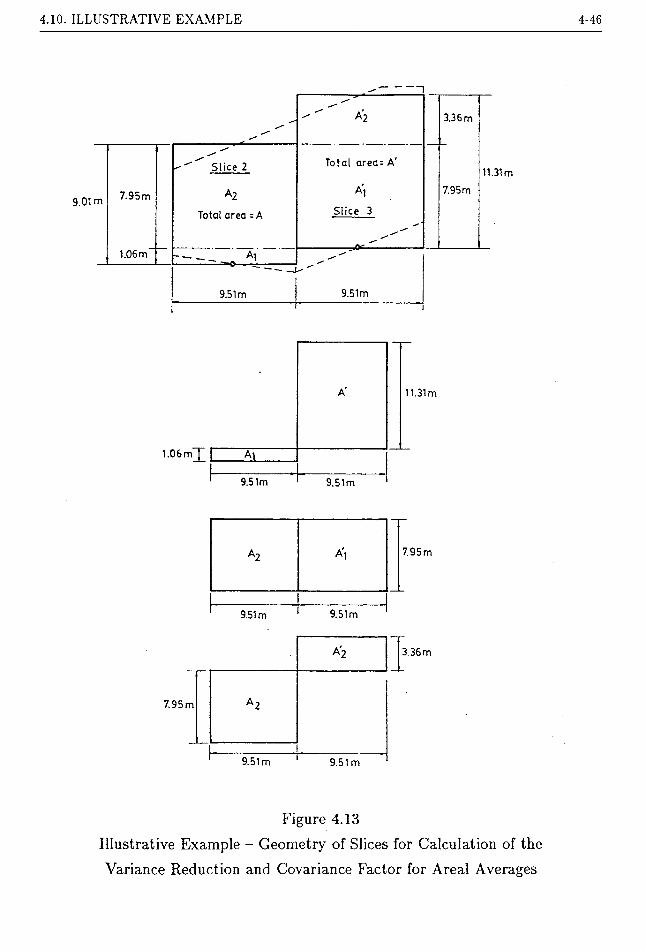
4.10. ILLUSTRATIVE EXAMPLE 4-46
-------- 1
3.36 m
Slice 2 11.31m7.95m7.95m9.01 m
Slice 3Total area = A
1.06 m
9.51m9.51m
1.06m~]~
A' 11.31m
l A,-
9.51m 9.51m
a2 Ai 7.95 m
9 51 m 9.51 m
A'2 3.36m
7.95 m A2
9.51 m 9.51 m
Figure 4.13Illustrative Example - Geometry of Slices for Calculation of the Variance Reduction and Covariance Factor for Areal Averages

4.10. ILLUSTRATIVE EXAMPLE 4-47
Using the formula in Table C.l in Appendix C, T2(L) is as follows
. f cosO0 sinO0 'l 1^ = Hr+ —1 =3
r2{L) = +9.51 2 x 9.512
= 0.27
(«' -1)
Similarly
_ f cos 90° sin 90° 'j 1 ~ | 3 * 1 } = 1
r 2(H) = — +v 1 9.01
= 0.10
1-
2 x 9.012 (C -1)
Therefore, r2(A) = 0.27 xO.l = 0.03. The variance of the sample spatial average
density over slice 2 becomes
var{iA} = s2 + r2M) J = i-52 jg + 0.031 = 0.34(kN/m3)2
c) Case 3
The configuration of slices 2 and 3 can be decomposed into two basic config
urations as shown in Fig.4.12. Let us consider the first basic configuration - lines
AB and BC. This configuration corresponds to the configuration of case 8 in Table
C.2 in Appendix C. From Fig.4.12, the following parameter values for the formula
can be derived, viz,
v%o — 9.51

4.10. ILLUSTRATIVE EXAMPLE 4-48
Vy0 = 1.00
0 \ = 6.02°
02 = 18.20°
Lx = 9.56
L2 =3.21
1sin(6.02° + 18.20°)
= 2.44
The constants of the integral in Eqn.4.25 are given as (Table C.2)
Ai = vxo — L\ cos61 = 9.51 — 9.56 x cos6.02° = 0.00
B{ — cot Ox = cot 6.02° = 9.48
Cx = vxo + L2 cos 02 — 9-31 + 3.21 x cos 18.20° = 12.56
Dx = - cot 02 = - cot 18.20° = -3.04
Ex = 0.0
F\ = Lx sin Ox = 9.51 x sin 6.02° = 1.00
Using the formula for I in Table C.4 in Appendix C for Type I ACF, we obtain
lx = 0.18. Similarly, I2 = 0.40. Therefore,
B(L, L\) = jUh + h)
2.449.56 x 3.21
• (0.18 + 0.40)
= 0.046
The second basic configuration in Fig.4.12 corresponds to the mirror image of case
7 in Table C.2. To use the formula, the local axes have to be changed as shown in

4.10. ILLUSTRATIVE EXAMPLE 4-49
Fig.4.12. The parameter values of the formula are as follows.
vxo = 21.49 - 11.97 = 9.51
vy0 = -3.75 - (-6.88) = 3.13
6{ = 18.20°
02 = 6.02°
h = 6.8
L2 = 9.56
1m — ________________ — 2 441 sin( 18.20° + 6.02°)
The constants for the integral /t can be calculated from the formulae of case 7 in
Table C.2 and using the expression for / in Table C.4, we obtain ^ It = 0.013.
Therefore
2.449.56 x 6.81
x 0.013 = 0.0005
The covariance factor B(L, L') can be obtained from the following procedure.
{ L' Lo )cov{cL,cL/} = covl cL, -jjcL/ + -JjtL'z >
_ ^ l r ~ , . ^2 r= —cov{cL, cL/ } -f -y7Cou{cL, cL^}U
= ^ ■ a- ■ B(L, L\) + ^ • a2 • B(L, L'2)
But cov{cl, cl>) = a2 • B(L, L'). Therefore
B(L, V) = B . B{L, L[) + ^- B(L, L'2)
3.21 x 0.046 + 6.81 x 0.000510.01
= 0.015

4.10. ILLUSTRATIVE EXAMPLE 4-50
The covariance of the sample spatial average cohesive strength becomes
cov{cL,cL>} = s2 £')}
|= 14.0(kN/m2)2
d) Case 4
Using equivalent rectangles, slices 2 and 3 can be decomposed into 3 basic
configurations as shown in Fig.4.13. Consider the first configuration - rectangles
Ai and A'. The covariance factor for this configuration can be evaluated using
Eqn.4.33. From Figures 4.8 and 4.13, the parameter values for the formula are
L*0=0
L\ = 9.51
L\ = 19.02
L% =9.51
H*0= 0
H* = 11.31
HZ = 12.37
H* = 1.06
= 102 / - +0.015l8
The calculations of Eqn.4.33 are shown in the following Table.
As a separable ACF is used, the variance reduction factor r2(AtJ) is calculated
using Eqn.4.30. For example, r2(Au) = r2(Lj) • T2)//*). The covariance factor
B(Ai, A') is given by
B(AUA')1
4AXA'

4.10. ILLUSTRATIVE EXAMPLE 4-51
i J 4* r2M.,) (-ly+ULtHf)2 -r2(Aij)
0 0 0.0 0.0 - 0.00
0 1 0.0 11.31 - 0.00
0 2 0.0 12.37 - 0.00
0 3 0.0 1.06 - 0.00
1 0 9.51 0.0 - 0.00
1 1 9.51 11.31 0.0225 259.91
1 2 9.51 12.37 0.0206 -285.45
1 3 9.51 1.06 0.15 14.94
2 0 19.02 0.0 - 0.00
2 1 19.02 11.31 0.0123 -568.30
2 2 19.02 12.37 0.0113 624.12
2 3 19.02 1.06 0.1465 -32.69
3 0 9.51 0.0 - 0.00
3 1 9.51 11.31 0.0225 259.91
3 2 9.51 12.37 0.0206 -285.45
3 3 9.51 1.06 0.15 14.94
sum=1.97
Table 4.3. Some Results for Calculating the Covariance Factor.

4.10. ILLUSTRATIVE EXAMPLE 4-52
1“ 4 x (9.51 x 1.06) x (9.51 x 11.31)
= 0.0005
x 1.97
The covariance factor for the second basic configuration can be obtained us
ing Eqn.4.32 and the third by repeating the procedure above. The values are
B(A2, A[) = 0.0117 and B(A2, A'2) = 0.0009. The covariance factor B(A, A') can
be obtained using the following procedure.
cov{7A,7A/} = cou{7Ai+A2,7A/}
r A\ _ A2 ~ ~ x= cov{ — iAl + —7a2,7a'}
= ^-cov{iAl,7A'} + ^-cov{7A2,7A/}
At A2A\= ^cov{ 7a157a'} + ^-^{7^,7^-} +
= -± • a2 ■ B(Ai,A/) 4- • cr2 • B(A2, AA'x) +
cov{7a2,7a;}
A2A2 2AA' a ■ B(A2, Aa> )
But cov{7A,7A'} = • B(A, A'). Therefore,
B(A, = B(AUA') + AA> • B(A2, Aa.) + ^ • B(A2, Aa.JAA'
= 0.002
and
cov{'ia,'1a-} = s2 + B(A, A1)
I = 0.3
For line averages, the uncertainty associated with the inherent variability,
measured in terms of the contribution to the variance of the sample spatial average,
is comparable to the sampling uncertainty associated with the estimation of the
= 1.52 x /- +0.002l8
4.10. ILLUSTRATIVE EXAMPLE 4-53
mean trend for this example. Therefore, none of the components can be neglected
in the analysis in the calculation of variance of the average cohesive strength.
However, because the soil density is averaged over a larger spatial domain, the
variance reduction from spatial averaging is significant. The uncertainty of the
sample spatial average soil density is dominated by the sample uncertainty as
shown in the example where the variance and covariance of the spatial averages
are only a small fraction of the sample point variance s2. If the soil properties are
modelled as perfectly correlated variates, the variance reduction and covariance
factor of the sample spatial average will be equal to 1 and hence the variance
and covariance of the sample spatial averages will be grossly over-estimated. This
explains why many of the analyses in the current literature give an unrealistically
high value of failure probability of slopes.

CHAPTER 5
STRUCTURAL ANALYSIS OF SOIL DATA
5.1 INTRODUCTION
In the previous chapter, the principles of probabilistic characterization of soil
profiles were discussed. In particular, the importance of the correlation structure
of soil properties and the role it plays in spatial averaging were emphasized.
This chapter addresses the estimation of the statistical parameters of soil prop
erties. In geostatistics, the statistical analysis of mining data is called a ‘structural
analysis’ which means extracting the statistical structure of the governing random
process from the data. This term will also be used herein. The structural analysis
of soil data is a vast subject in its own right and its development lags far behind the
theoretical development of geostatistics or random field. It is fair to say that the
autocovariance function (ACVF), autocorrelation function (ACF) or variogram of
soil properties is still commonly estimated using some semi-empirical procedures
such as fitting by ‘eye’. Active research in the field of structural analysis of soil
data only started in the 1980s and is still in a stage of development. Ripley (1981)
also commented in his book that very little work has been done on fitting the
parameter of the ACVF. The statement is still true. This chapter is an overview
of the recent theoretical developments in the subject. The implications of some
of the theories to the practice of soil sampling in the field are highlighted. Some
5-1

5.2. TYPE I SOIL PROFILES 5-2
of the geostatistical approaches relevant to the structural analysis of soil data will
also be mentioned.
Not surprisingly, the volume of literature on structural analysis of soil data
decreases in the order of Type I, Type II and Type III soil profiles, in agreement
with the complexity of the problem.
Before commencing a structural analysis of soil data, it is useful to carry out
an exploratory data analysis (EDA) to detect any anomaly that may be present
in the data. Cressie (1983) gave a good discussion of such a procedure.
The statistical analysis and interpretation of geotechnical data requires skills
and experience which can only be built up through practice. Although in many
cases the analysis can be automated using computer programs, the results must
not be accepted without cross validation with the observed data. The experience
of the the mining engineers in the statistical analysis of mining data such as David
(1977) and Journel and Huijbregts (1978) is very useful.
5.2 TYPE I SOIL PROFILES
To characterize a Type I soil profile, the mean value, the point variance, the
autocorrelation function and the trend variance (which is also the variance of the
sample mean value for a Type I soil profile) of the soil property are required. Three
sets of data will be used to illustrate the procedure of structural analysis of soil
data of a Type I profile. Details of the data are summarized in Appendix F. In
the following, the first set of data will be represented by the symbol the second
by o and the third by •.
5.2.1 Estimation of mean value
Given N samples of K(t{) at location £t, i = 1, N in the field, the mean value
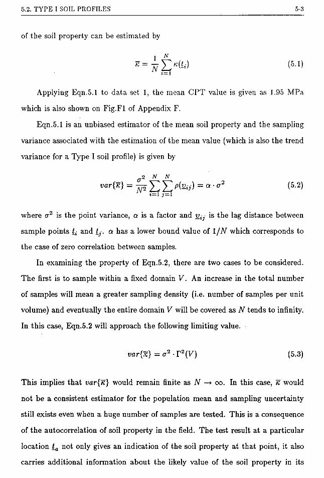
5.2. TYPE I SOIL PROFILES 5-3
of the soil property can be estimated by
(5.1)
Applying Eqn.5.1 to data set 1, the mean CPT value is given as 1.95 MPa
which is also shown on Fig.Fl of Appendix F.
Eqn.5.1 is an unbiased estimator of the mean soil property and the sampling
variance associated with the estimation of the mean value (which is also the trend
variance for a Type I soil profile) is given by
where a2 is the point variance, a is a factor and vt] is the lag distance between
sample points lt and tj. a has a lower bound value of l/N which corresponds to
the case of zero correlation between samples.
In examining the property of Eqn.5.2, there are two cases to be considered.
The first is to sample within a fixed domain V. An increase in the total number
of samples will mean a greater sampling density (i.e. number of samples per unit
volume) and eventually the entire domain V will be covered as N tends to infinity.
In this case, Eqn.5.2 will approach the following limiting value.
This implies that var{K} would remain finite as N —► oo. In this case, k would
not be a consistent estimator for the population mean and sampling uncertainty
still exists even when a huge number of samples are tested. This is a consequence
of the autocorrelation of soil property in the field. The test result at a particular
location ta not only gives an indication of the soil property at that point, it also
carries additional information about the likely value of the soil property in its
a2 N N(5.2)
var{:c} = a2 ■ r2(K) (5.3)

5.2. TYPE I SOIL PROFILES 5-4
vicinity. Hence, an extra test carried out very near to ta will only give very limited
additional information about the population mean value of the soil property over
the entire field.
The second way of soil sampling is to increase the sampling domain V as N
increases. For soil sampling at a gridded network with fixed grid size, this would
mean an expansion of the network in space. In this case, Eqn.5.2 will have an
asymptotic value of order 1 /N for well behaved ACF (i.e. ACF which diminishes
sufficiently fast with an increase in lag distance) and 7c would become a consistent
estimate of the population mean.
Of course, the concept of an infinitely large domain exists only in theory.
In practice, the spatial domain would be finite, being the dimension of the site.
But the implication of the above discussion is that in a site investigation, an
extensive sampling of soil specimens over a small area within the site is not a
cost effective way of soil sampling as far as the estimation of the mean value is
concerned. Given a fixed number of soil specimens to be taken from the field, it
is preferable to maximize the separation distances between the samples, taking
specimens from different parts of the entire site rather than concentrating on a
particular small area within the site. If the site dimensions are of the order of
the scale of fluctuation, it has to be recognized that the ‘site mean’ may be the
different to the true population mean.
Figures 5.2 to 5.5 show the variation of the factor a in Eqn.5.2 for equally-
spaced data as shown in Fig.5.1. For a fixed value of A1/6, an increase in N would
mean an increase in the sampling length. By overlapping the different graphs, it
can be observed that the difference in a between different ACFs is small.
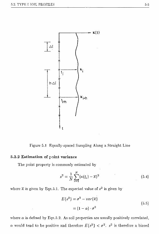
5.2. TYPE I SOIL PROFILES 5-5
Figure 5.1 Equally-spaced Sampling Along a Straight Line
5.2.2 Estimation of point variance
The point property is commonly estimated by
1s2 = (5.4)
1 = 1
where k is given by Eqn.5.1. The expected value of s2 is given by
E{s2} — a2 — uar{7c}
= (1 — a) ■ a2(5.5)
where a is defined by Eqn.5.2. As soil properties are usually positively correlated,
a would tend to be positive and therefore E{s2} < a2. s2 is therefore a biased

5.2. TYPE I SOIL PROFILES 5-6
Type I ACF
30 40 80 90 100sample
Figure 5.2 a Factor for Type I ACF
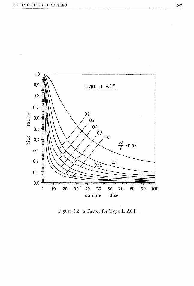
5.2. TYPE I SOIL PROFILES 5-7
Type II ACF
/ 0.6
. • t 1 < r i i | < i • . . k | , . . , , .. , 1, , , , , , , , , i | , , . , |, , . . , I
10 20 30 40 50 60 70 80 90 100sample size
Figure 5.3 a Factor for Type II ACF
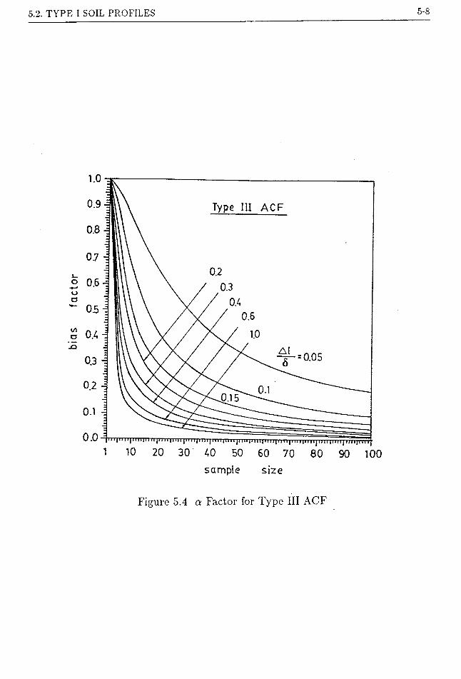
5.2. TYPE I SOIL PROFILES
1 10 20 30 40 50 60 70 80sample size
Figure 5.4 a Factor for Type III ACF
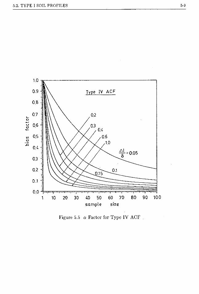
5.2. TYPE I SOIL PROFILES 5-9
Type IV ACF
80 90 10060 70sample size
Figure 5.5 a Factor for Type IV ACF

5.2. TYPE I SOIL PROFILES 5-10
estimator, consistently underestimating the point variance a2. The bias term,
which is equal to the theoretical variance of 7c, is of order l/N when N is large.
Therefore, s2 is an asymptotically unbiased estimator of a2.
It can be seen from Figures 5.2 to 5.5 that the bias is significant if the sample
size is small and increases with a decrease in the value of A1/6. Knowing the
ACF of the soil property, the bias can be easily accounted for by multiplying s2
by a factor of 1/(1 — a). The corrected estimator of point variance, denoted by s2
hereafter, will be given as
(l-a)(5.6)
In particular, if the sample locations are far apart, the samples can be regarded
as statistically independent. In this case, a = l/N and s2 becomes the usual
unbiased estimator given by Eqn.4.58.
A question often of interest is what strategy should be used to minimize the
value of a and the variance of s2 in a site investigation program. For a fixed A1/6
ratio, the longer the sampling length (i.e. more samples) is, the smaller will be the
value of a as indicated by Figures 5.2 to 5.5. The same is also true for the variance
of s2. A more common requirement is to determine the number of soil samples to
be taken for a fixed sampling length. A typical example is a site investigation for
a pile design in which soil samples would normally be taken over a depth roughly
equal to the anticipated design length of the pile.
Fig.5.6 shows the variation of the a against the number of samples taken
within a fixed sampling length of 4 x 8. The a factor drops initially as the sampling
size increases (i.e. a smaller sampling interval). However, when the sampling
interval decreases to about half of the scale of fluctuation, a further increase in
the sample size gives almost no change to the value of a. Also shown in the figure
is the variance of s2, var{s2}, which is calculated under the assumption that the

5.2. TYPE I SOIL PROFILES 5-11
sampling length = 46
var{ s2}
10 20 30 40 50 60 70 80 90 100number of samples
Figure 5.6 a Factor and var{s2} for a Fixed Sampling Length
soil property follows a joint Gaussian distribution and the point variance is unity.
Again, the threshold vale of a is about half of the scale of fluctuation. Therefore,
as far as the precision of the estimation of the mean value and the point variance
is concerned, there is no advantage in reducing the sampling interval to less than
half of the scale of fluctuation. The only way to reduce the alpha factor is to
sample over a greater length. However, in order to estimate the ACF of the soil
properties, it is necessary to have samples taken at sampling intervals less than
this value.
Based on the above observations, a useful strategy in soil sampling is as follows:
1. An inexpensive test is used to measure a property of the soil (e.g. cone resistance

5.2. TYPE I SOIL PROFILES 5-12
from a CPT or index properties) at close spacings. This would enables the ACF
of the property to be estimated with sufficient precision. The ACF so obtained
can be taken as indicative of the ACF of other properties of the soil.
2. Samples can then be taken at a larger spacings from the field so that tests
can be performed to determine the soil parameters (e.g. strength, density etc)
which are required as input parameters in the analysis. The spacing should
preferably be larger than the scale of fluctuation to minimize the correlation
of samples so that the value of a would become near to its minimum value of
l/N.
For data set 1, the value of s2 is obtained as 0.139 (MPa)2. As will be discussed
later, the autocorrelation of cone resistance for data set 1 is well described by a
Type I ACF with a scale of fluctuation of 0.2m which also implies from Fig.5.2 a
value of 0.12 for the factor a. Using Eqn.5.6, the corrected variance estimate is
given as
*2 = (r^=0157<MPa>2
The corrected standard deviation s is shown on Fig.Fl of Appendix F. As the
sampling length is large compared to the scale of fluctuation, the bias of s2 is not
significant for this case.
5.2.3 Estimation of trend variance
If the point variance of the soil properties is known, the trend variance can
be estimated using Eqn.5.2. As discussed in the previous section, the a factor and
point variance for data set 1 are respectively 0.12 and 0.157 (MPa)2. The trend
variance is therefore given as
var{lc} = 0.12 x 0.157 = 0.019(MPa)2
Some difficulties arise in the simultaneous estimation of the cohesion and
5.2. TYPE I SOIL PROFILES 5-13
coefficient of frictional resistance of the soil at a point. One way to obtain tfre
strength components of the soil from one sample is to perform a multi-staged test.
In this case, the procedure of structural analysis for the strength parameters would
be the same as that discussed above for the CPT data. However, it is not always
practical to carry out a multi-staged test for soil samples.
An alternative way is to carry out shear tests for samples close to each other
in the field, e.g. neighbouring soil specimens trimmed from the core of a borehole.
If the samples are close together, the strengths can be regarded as perfectly cor
related and the strength parameters obtained from these samples will constitute
a single observation in the statistical sense. However, there are seldom sufficient
soil specimens close enough to each other to justify the above assumption. This is
particular true when the scale of fluctuation is small. For instance, if the scale of
fluctuation of the soil property is of the order of a few decimeters (10cm), which
is not uncommon in real situations (for example, the CPT data above), soil speci
mens 0.5m apart may be regarded as independent samples even though they may
be very close physically. In this case, the test results have to be aggregated and
the mean cohesion and tan (f> obtained from the regression analysis of the p-q plot
of the data.
As a side product of regression analysis, the variances of the y-intercept and
of the gradient of the straight line in the p-q plot can also be obtained. These
variances are in turn related to that of the cohesion and tan </>. However, it must
be pointed out that the variances of cohesion and tan (f) so obtained are not the
point variances of the soil properties. They represent only the trend variance
var{7c} associated with the estimation of the mean cohesion (which is related to
the intercept) and mean tan</> (the gradient). Thus lumping all the test results
in a single p-q plot does not give the estimate of the point variance of the soil

5.2. TYPE I SOIL PROFILES 5-14
property. Accordingly, the variance of the sample spatial average will be given as
var{KV} = a2-T2(V) + a2eg (5.7)
where a2eg is the variance of the sample mean property obtained from regression
analysis.
As lumping the test results does not enable the point variance to be obtained,
a judgemental vale based on local experience of the soil properties will have to be
used for the point variance a2. This is not as discomforting as it may seem because
any uncertainty in the estimation of a2 is scaled down by a factor of r2(K). For
a soil with a small scale of fluctuation, the dimensions of the slope may be such
that the uncertainty is dominated by the sampling uncertainty making an accurate
estimation of point variance a2 unimportant.
5.2.4 Estimation of correlation structure
To estimate a truly three dimensional ACF, a prohibitively large number of
samples is required. For one dimensional ACF, it has been suggested by Lumb
(1974) that a minimum of 20-50 samples are required to give a reliable estimate
of the ACF. Similar figures have also been quoted for mining data in Journel and
Huijbregts (1978). Therefore, for a truly three dimensional ACF, this will mean a
sample size of the order of 104 to 105 which can hardly be possible in practice.
A more practical approach is to assume a separable correlation structure for
the soil properties. In consequence,
Pin) =Pi(Ui) ' P2(v2) -P3(vi) (5.8)
where Vj, v2 and are the lag distance in the principal directions. The as
sumption of a separable correlation model leads to considerable simplifications.
Furthermore, the ACF can be estimated separately using a smaller number of soil
measurements taken along the principal directions.

5.2. TYPE I SOIL PROFILES 5-15
At present, published results on the ACF of soil properties are usually limited
the principal directions (see Table 4.2). This assumption may be reasonable for
fill embankments or clay deposits because the compaction or deposition of soils
usually follow a vertical sequence. If the ACF in different horizontal directions are
not dissimilar, a further assumption of circular symmetry may be made so that
Eqn.5.8 becomes
where the subscripts y and r denote vertical and radial lag distances.
For residual soil profiles on hillslopes, the weathering progress may process in
a direction normal to the slope face. It is likely that that principal directions are
normal and parallel to the slope face. However, little has been published on the
ACF of residual soils and hence no conclusive remark can be made at this stage.
Other anisotropic autocorrelation models have been considered by David (1977)
and Journel and Huijbregts (1978). The process of constructing an autocorrelation
model is also well illustrated in these two references.
5.2.4.1 Sample ACVF
To get a ‘feel’ for the correlation structure of the soil properties, it is common
to plot the variation of the sample estimate of the ACVF with lag distance. The
resulting graph is called a sample ACVF.
The ACVF is commonly estimated by one of the following two estimators.
to the vertical and the horizontal directions which are commonly regarded as
p(v) = py(vy) ■ Pr(vr) (5.9)
(5.10)
(5.11)
where N is the total number of samples used for the estimation of k (Eqn.5.1)
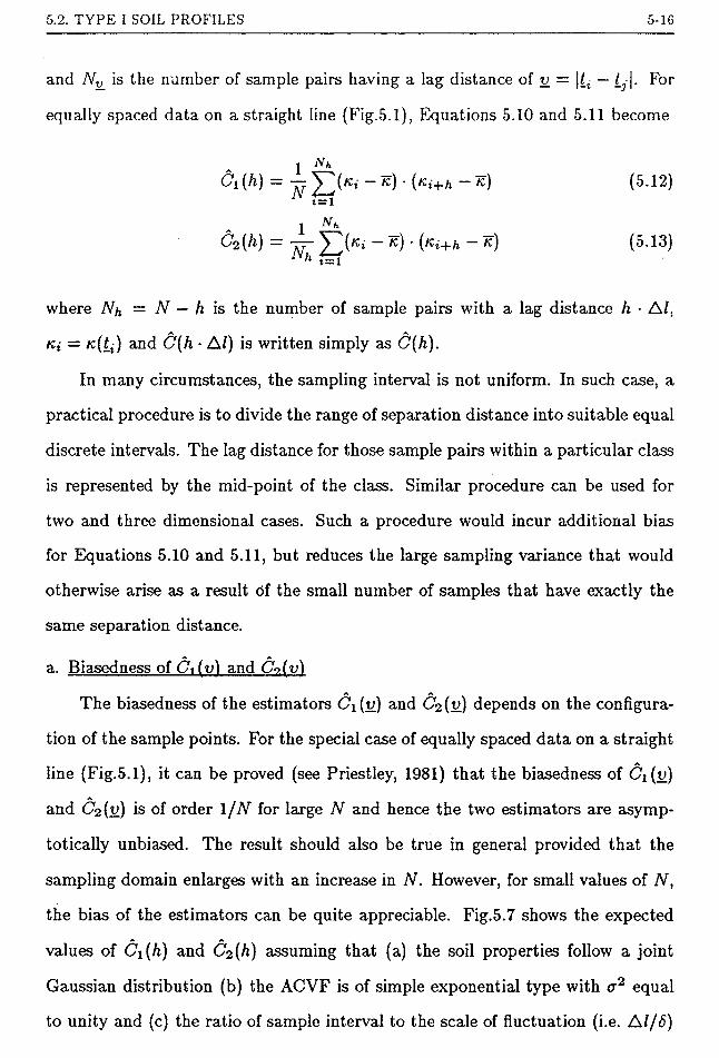
5.2. TYPE I SOIL PROFILES 5-16
and Ny_ is the number of sample pairs having a lag distance of v = |/t — L\. For
equally spaced data on a straight line (Fig.5.1), Equations 5.10 and 5.11 become
j Nh
Ct(h) = — - ?c) • («<+* - K) (5.12)1= 1
1C2(h) - — ^(/c* - 7c) • (Ki+h ~ k) (5.13)
where Nh = N — h is the number of sample pairs with a lag distance h • A/,
Ki — K(ii) and C'f/i • A/) is written simply as C(h).
In many circumstances, the sampling interval is not uniform. In such case, a
practical procedure is to divide the range of separation distance into suitable equal
discrete intervals. The lag distance for those sample pairs within a particular class
is represented by the mid-point of the class. Similar procedure can be used for
two and three dimensional cases. Such a procedure would incur additional bias
for Equations 5.10 and 5.11, but reduces the large sampling variance that would
otherwise arise as a result of the small number of samples that have exactly the
same separation distance.
a. Biasedness of C\ (t>) and Co(v)
The biasedness of the estimators Ci(v) and C2{u) depends on the configura
tion of the sample points. For the special case of equally spaced data on a straight
line (Fig.5.1), it can be proved (see Priestley, 1981) that the biasedness of C\(y)
and C2 (^) is of order 1 /N for large N and hence the two estimators are asymp
totically unbiased. The result should also be true in general provided that the
sampling domain enlarges with an increase in N. However, for small values of N,
the bias of the estimators can be quite appreciable. Fig.5.7 shows the expected
values of C\(h) and C2(h) assuming that (a) the soil properties follow a joint
Gaussian distribution (b) the ACVF is of simple exponential type with a2 equal
to unity and (c) the ratio of sample interval to the scale of fluctuation (i.e. A//<5)
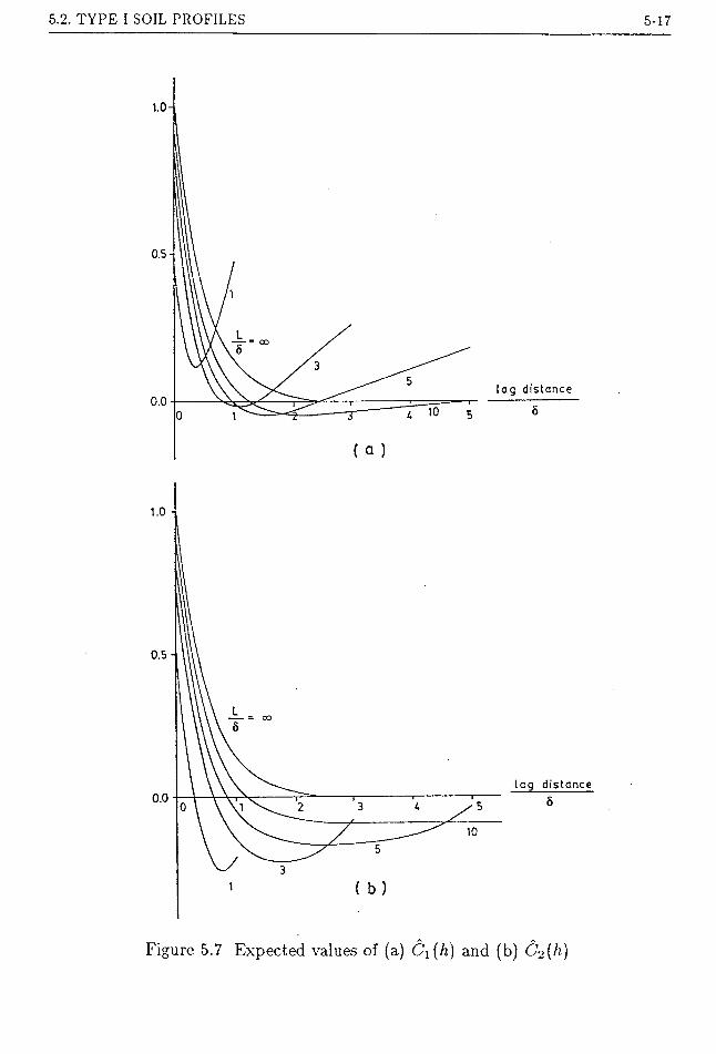
5.2. TYPE I SOIL PROFILES 5-17
lag distance
6
lag distance 6
Figure 5.7 Expected values of (a) C\(h) and (b) Co(h)

5.2. TYPE I SOIL PROFILES 5-18
is 0.1. L/b in the figure denotes the ratio of the total sampling length to the scale
of fluctuation. Since Al/b = 0.1, a value of L/6 — 1 will imply a total sample size
of 11 and so on. It can be seen that sample ACVF based on a small sample size
is highly biased.
To reduce the bias of the sample ACVF, Cressie and Glonek (1984) and Cressie
and Hawkins (1984) have recently proposed an alternative estimator
1 N*
C3(h) = — y^(/c» - med(/Cj)) • (/cl+/l - med(/c;)) (5.14)
where med(-) is the median of the test results. Eqn.5.14 has the implicit assump
tion that the distribution of the point property is symmetrical,
b. Variance and covariance of Ci (t>) and Cr>(v)
The derivation of the variance and covariance of the estimators Ci(v) and
C2{v) requires the additional assumption that /c(£) is stationary up to the fourth
order, i.e.
C{kUi)k((2)k(<3)k(<4)}
is a function of the lag distances — /2|, \Li — etc. Here discussion will only be
confined to the special case of equally spaced data along a straight line (Fig.5.1).
The covariance of the estimator C\ (h) for a Gaussian process is given as
(Priestley, 1981)
I —n iy — n — s
eW{c,(A),Cl(A + «)} = ;p g V [C(j - i)C(j + s-i)
+ C(j + h + a - i)C(j - i - h)\
(5.15)
Setting s = 0 and assuming a Gaussian process, the following expression for
the variance of C\(h) is obtained.
N-h-l
E ,r= — (N — h — l)
var {6,(/i)} = ^ E* (Af — A — |r|) • |C2(r) + C(/j + r)C(A — r)| (5.16)
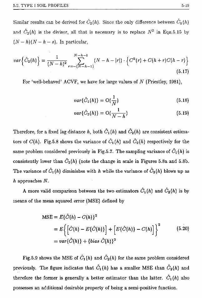
5.2. TYPE I SOIL PROFILES 5-19
Similar results can be derived for C2(h). Since the only difference between C\(h)
and C2(h) is the divisor, all that is necessary is to replace N2 in Eqn.5.15 by
(N — h)(N — h — s). In particular,
var{62(h)} = * £ (N-h-\r\).{C*(r) + C(h + r)C(h-r)}
(5.17)
For ‘well-behaved’ ACVF, we have for large values of N (Priestley, 1981),
var{Ci(h)} = O(-L) (5.18)
var{C2(h)} = 0(^-) (5.19)
Therefore, for a fixed lag distance h, both C\(h) and C2(h) are consistent estima
tors of C(h). Fig.5.8 shows the variance of C\(h) and C2(h) respectively for the
same problem considered previously in Fig.5.7. The sampling variance of C\(h) is
consistently lower than C2(h) (note the change in scale in Figures 5.8a and 5.8b.
The variance of C\(h) diminishes with h while the variance of C2(h) blows up as
h approaches N.
A more valid comparison between the two estimators C\(h) and C2(h) is by
means of the mean squared error (MSE) defined by
MSE = E{C(h) - C(h)}2
= eI [6(h) - £{C(/i)}] + [E{C(h)} - C(h)
= var{C(h)} + {bias C(h)}2
(5.20)
Fig.5.9 shows the MSE of C\[h) and C2(h) for the same problem considered
previously. The figure indicates that C\(h) has a smaller MSE than C2(h) and
therefore the former is generally a better estimator than the latter. Ci(h) also
possesses an additional desirable property of being a semi-positive function.

5.2. TYPE I SOIL PROFILES 5-20
lag distance
6
-f- = 1
lag distance
6
Figure 5.8 Sampling Variance of (a) C\(h) and (b)

5.2. TYPE I SOIL PROFILES 5-21
Figure 5.9 Mean Square Error of C\(h) and Co(h)

5.2. TYPE I SOIL PROFILES 5-22
As the sample estimates of C(h) at different lag distances are obtained from
the same set of data, the estimates are correlated as indicated by Eqn.5.15. For
‘well-behaved’ ACVF, Eqn.5.15 would also approach zero as N —► oo. However,
for small value of N, the correlation will be fairly high. In consequence, ‘ripples’
may appear in the sample ACVF and the curve may not decay as quickly as the
parent ACVF. This is a further complication in the interpretation of the sample
ACVF.
5.2.4.2 Sample ACF
The graph of sample estimates of the ACF with lag distance is called a sample
ACF or correlogram. Since the ACF p(v) is related to the ACVF by
p(u) =
natural choices of the estimator will be
Pi(h) =
M10 =
Cfe)0(0)
c'Ait)
C,(0)
Ci(h)<3-2(0)
(5.21)
(5.22)
(5.23)
The statistical properties of pi(h) and p2(/i) are even more complicated than
Ci(h) and C2(/i). No exact results have yet been derived for the two estimators.
However, for large N, approximate expressions for the covariance of p\(h) and
p2(/i) are given in Bartlett (1946) and Priestley (1981). The behaviour of p\(h)
and p2(/i) is similar to that of C\{h) and C2(/i).
Another estimator of the ACF which has been used in the past is the sample
correlation coefficient
N-h _ _(*1 “ *1 )(*•+* - «2>
P = i = l
N-h N-h' J2 {k% ~ *i)2 • (ac1+/i - 7c2);
i=1 t=l
(5.24)

5.2. TYPE I SOIL PROFILES 5-23
N-h _ N-hwhere Tci = JZ aRd = TjZk JZ Ki+h- The estimator has become ob-
solete for reasons given in Jenkins and Watts (1968) and Priestley (1981), namely
that it does not (a) fully utilize the stationary properties of n(t) and (b) yield a
positive semi-definite autocorrelation matrix.
5.2.4.3 Sample variogram
An alternative way to display the correlation structure of the soil properties
is by means of the sample variogram. Since
7(0 = 0(0) - C(v) (5.25)
the information on the correlation structure carried by 7(1;) and C[v) is essentially
the same. The autocorrelation of soil properties usually diminishes with lag dis
tance. Consequently, 7(u) will approached the point variance C(0) as v increase.
The point variance which is C(0) can therefore be estimated by the asymptotic
limit, also called the sill, of the sample variogram at large lag distance.
As the variogram is defined by
2l(v) = E{k{L) ~ *(*')}" (5-26)
where \t — l_'\ = v, a natural choice of the estimation for the semi-variogram 71 (h)
will be
N- 27i(li) = ^3{K(-*) — k(->)}2 (5-27)
where |ft — tj\ = v and Ny. is the number of sample pairs with lag distance v.
7i(n) due to Matheron (1971) is the earliest estimator proposed for 7(1;) and is
still widely used nowadays. For equally spaced data on a straight line (Fig.5.1),
7(t>) will be denoted simply as q(/i) and similarly for its estimators.
71 (u) is an unbiased estimator for 7(u). However, it is not a resistant estimator
in the sense that the value of (t>) is badly affected by outliers due to the square

5.2. TYPE I SOIL PROFILES 5-24
term in Eqn.5.27. Over the past few years, mining geostatisticans have proposed
many alternative resistant estimators for 7(1’). The following are some examples.
Armstrong and Delfiner (as reported in Dowd, 1983) have proposed two al
ternative estimators. The first one is
where Qq is a suitable quantile of the experimental cumulative distribution func
tion of the squared difference for lag h. For example, Qq can be chosen to be me
dian of the squared difference. The second estimator by Armstrong and Delfiner is
based on the M-estimator by Huber and iterations are required for the calculation
of the estimate.
Cressie and Hawkins (1984) proposed a series of estimators based on the trans
formed difference data Y{ — |/ct- — Act+/j|2. The estimators have the form
where T is an estimator for the central location of Tr. A number of estimators have
been used for this purpose including the mean, median, trimmed mean and .the
M-estimators. It is observed (Cressie and Hawkins, 1984) that the mean, median
and the M-estimators yield satisfactory results. However, the M-estimators are
more complicated and an iterative procedure is required for the calculation of T.
Dowd (1983) proposed four other resistant estimators for 7(h). The first two
estimators are
12(h) = (5.28)
1 T*(5.29)2 ' 0.457 + 0.494/N + 0.043/JV-
(5.30)
(5.31)

5.2. TYPE I SOIL PROFILES 5-25
where yt(h) = /ct — Kl+h and y(h) ^median of yt(h). The third estimator is
where wt = (/ct- - kl+h)/(K • Ml) and Ml = median |/cx —/ct+1|. The sum is over
all sample pairs (totalling Nh) with lag distance h and K is a constant depending
on the data, usually from 6 to 9, the same as for the fourth estimator 77(t>):
where = (yi(h) — y(h))/(K ■ M2) and M2 = median \yt(h) — y(h)|. yt(h) is
defined as in Eqn.5.31.
Omre (1983) has also developed another resistant estimator based on the
estimation of the bivariate probability density function of Kt and Kv+h-
Each proponent of the resistant estimators has demonstrated the superiority
of his own estimator(s), normally by means of simulated data. Perhaps it is fair to
say that each of the resistant estimators discussed above would be more resistant
at large to contamination by outliers than the classical estimator 71 (t>), but none
of the estimators will be resistant enough to be the most resistant estimator for
every possible form of contamination.
Cressie (1979) proposed a somewhat different approach based on straight-line
fitting for the estimation of the variogram. Define Dt^ — «,•+/, — Kt. Assuming a
second order stationarity and that Dl+k,i-k and A,/i+A: follow a bivariate Gaussian
distribution, it can be shown that
%{h) = (5.32)
. _ Nhj2(y'(h) - y(h))2 ■ U - w.2)4l7{n) — r -,22[E(l-»,2)'(l-5»r)
(5.33)
(5.34)
where E{X\Y} is the expectation of X given Y. Thus if a linear regression of
Di^+k against Dl+k,h-k is performed, a straight line through the origin with
gradient b — (7(h) — ~i{k))l^(h — k) would be expected.
5.2. TYPE I SOIL PROFILES 5-26
In particular, if k = h— 1, then b = (7(h) — 7(h— 1))/7(1) or 7(h) = 7(h— 1) +
6-7(1). By successively plotting the data points (Dl+h~ 1,1, Di^h-i), h = 1,2,-*
and calling 6^ the gradient of the best fit straight line through the origin, we have
7(2) = 6! • 7(1)
7(3) = 7(2) +62 • 7(1)
7(/i) =i(h- 1) + 62 • 7(1)
or
l(h) — (1 + 61 -f • • • + bh-i) • 7(1) (5.35)
The estimate of 7(h) can therefore be estimated by the recurrent relation of
Eqn.5.35. 7(1) can be estimated using any of the estimators mentioned above.
Similarly, by putting k = 1, we have
7{h) — (1 + Ch-i + Ch-i Ch-i + * * • + c/jC/i—i • • • Ci) -7(1) (5.36)
where Ch-1 is the gradient of the regression line of A,/i+i against Dt+\,h-\ etc.
The graphical method by Cressie (1979) is simple, but viable only when a
substantial amount of data is available. Taking h = 2 and k = h — 1 (Eqn.5.35),
it can be proved that the coefficient of correlation p between A+1,1 and D, 3 is
p(h) - p(2h)
1 - P(3A))(1 - p(h))(5.37)
Using the simple exponential model and writing f = exp{—2/iA//<5}, Eqn.5.37
becomes
sj 1 + f + f2f * 1 (5.38)
As ^ tends to 1} p approaches the theoretical asymptotic maximum value of 0.578.

5.2. TYPE I SOIL PROFILES 5-27
* * * — r
sample correlation coefficient
Figure 5.1095% Confidence Interval for Coefficient of Correlation p
Values of Curves are Number of Samples

5.2. TYPE I SOIL PROFILES 5-28
Fig.5.10 shows the 95% confidence interval for the experimental correlation
coefficient. Unless the sample size is large, the confidence interval is wide. For
example, for N = 20, the 95% confidence interval is approximately (0.2,0.8) for
the theoretical maximum value of p. This would imply a high sampling variance
for bh and the estimates of t(/i) will quickly become very unreliable as 7(h) is
built up successively using Eqn.5.35.
5.2.5 Parameter estimation of autocorrelation models
Both the sample ACVF (or ACF) and sample variogram are very useful in
choosing of a suitable autocorrelation model. Once a model is chosen, the next
step is the estimation of the parameters for the chosen model. Various methods
will be discussed, in the order of their complexity.
5.2.5.1 Fitting by ‘eye’
The procedure of fitting by ‘eye’ is widely used in geotechnical data analysis
and geostatistics (e.g. David, 1977; Journel and Huijbregts, 1978; Ripley, 1981)
because of its simplicity.
The procedure of fitting by ‘eye’ involves the fitting of a theoretical model to
the sample ACVF, correlogram or variogram. The selection of the parameter is
often based on the visual harmony between the fitted model and the experimental
curve. There are various ways by which the autocorrelation model can be fitted.
The following are some examples.
Fig.5.11 shows a plotting paper for the fitting of a simple exponential ACF.
To use the graph, the sample ACF (Eqn.5.22) is plotted against the lag number.
The value of A//<5 which gives the best fit to the sample ACF is read from the
graph. Knowing the sampling interval A/, the scale of fluctuation can be evaluated
accordingly.
The sample ACFs of data sets 1 and 2 are also plotted in Fig.5.11 using the
estimator p\(h) (Eqn.5.22). The curve with A//<5 = 0.1 gives a satisfactory fit

5.2. TYPE I SOIL PROFILES 5-29
Figure 5.11 Plotting Paper for Type I ACF

5.2. TYPE I SOIL PROFILES 5-30
to both data sets. As A/ is 0.02m for data set 1 and 2m for set 2, the scales of
fluctuation are therefore given respectively as 0.2m and 20m.
Another commonly used technique of fitting is by matching the gradient of the
experimental and theoretical curves at zero lag. The gradient of the experimental
ACF can be estimated by fitting a straight line to the first few points of the curve.
For example, fitting a straight line to the first five data points of Fig.5.11 for data
set 2 yields an estimate of —0.18 for the gradient of the experimental ACF at zero
lag. Since p(h) = exp{—2hAl/8}, we have
dp(h) _ 2A / dh &=o 6 (5.39)
Therefore,
-0.18
=> 8
2A /T
2x20.18 = 22m
which is similar to the estimate obtained previously for data set 2.
As fitting a straight line is always easier than fitting a curve, it is preferable,
if possible, to perform a suitable transformation to produce a linear relationship.
For instance, the simple exponential ACF will appear as a straight line on a semi
logarithm plot as illustrated in Fig.5.12 for the data set 1 and Fig.5.13 for data set
2. The gradient of the fitted straight linesfby eye) are —9.4 and —0.21 respectively
which correspond to a <5 of 0.21m for data set 1 and 19m for data set 2.
For more complex models involving more than one parameter, further manip
ulation of the data may be necessary. Examples of this can be found in David
(1977) and Journel and Huijbregts (1978).
5.2.5.2 Variance plot
The method of variance plot to be discussed in this section is also based on a
procedure of fitting by ‘eye’. But the method involves a more in-depth theoretical
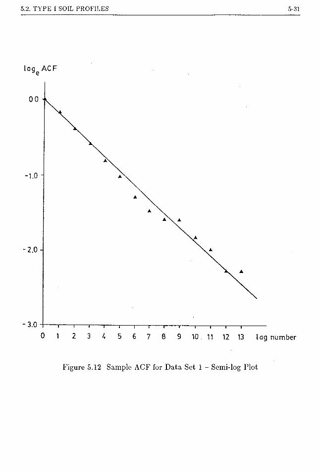
5.2. TYPE I SOIL PROFILES 5-31
loge ACF
-1.0 -
-2.0 -
10 11 12 13 lag number
Figure 5.12 Sample ACF for Data Set 1 - Semi-log Plot
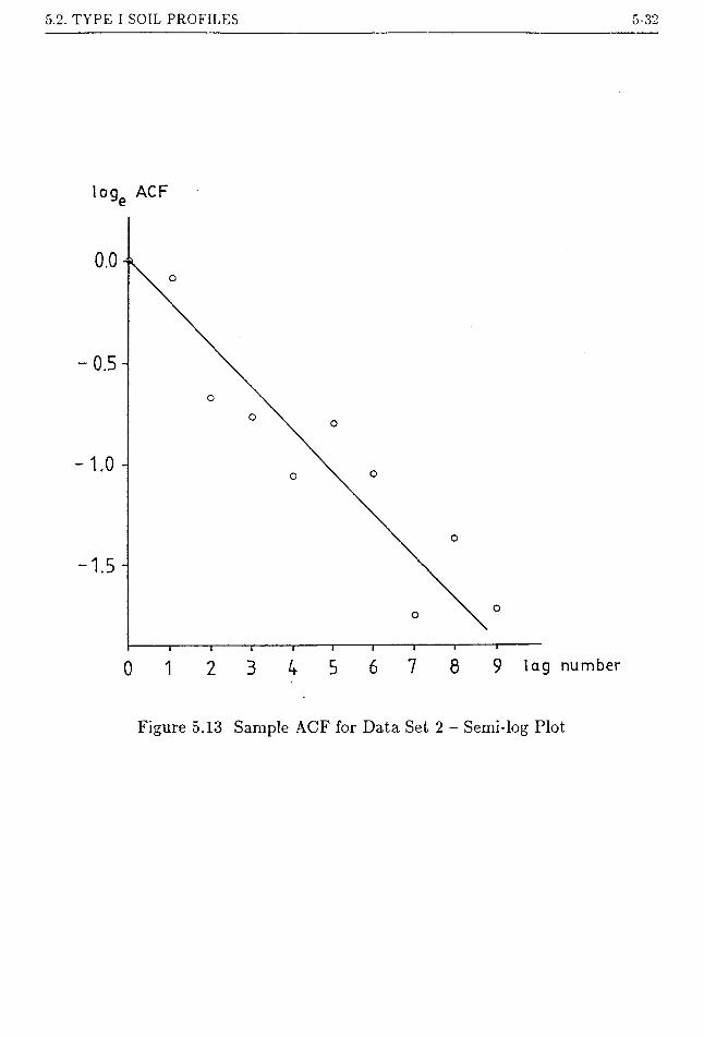
5.2. TYPE I SOIL PROFILES 5-32
1 o ge ACF
-0.5-
-1.0 -
-1.5 -
9 lag number
Figure 5.13 Sample ACF for Data Set 2 - Semi-log Plot

5.2. TYPE I SOIL PROFILES 5-33
consideration which deserves a separate discussion.
Agterberg (1967) appears to be the first to apply the technique of variance
plot to the structural analysis of mining data. The method is also discussed in
his book Agterberg (1974). A similar procedure was also proposed by Vanmarcke
(1977a&c) for the estimation of the scale of fluctuation of soil properties. Define
K1 n —ln
n
^ ^ Ki+k— 1 (5.40)
7cm is simply the average of n adjacent observations starting from Act. Consider the
theoretical variance <r2 of 7cm of a equally-spaced spatial series (Fig.5.1). According
to the assumption of stationarity, uar{7c;n } is independent of the location. Without
loss of generality, take t = 1. Thus
K = var{lcln}j n n i—1
— {^%qr{/Ct} + y]co^{/Ci,/ct+J}|
2 9 n *—1(5.41)
= a2 -rz(n)
n—1where T2(n) = £ jl + 2 (1 — ^-)/?(r). In fact, the a factor discussed earlier
in Section 5.2.1 is T2(N) where N is the total number of samples. Note T2(n) is
analogous to the variance reduction factor for the continuous case and hence the
same symbol is used here. r2(n) has similar characteristics as T2(L), namely
1 if n = 1
^ if n is larger2(n) = (5.42)
where 6n is a constant related to the scale of fluctuation 6 and it can be treated
as the scale of fluctuation for the discrete case. For the simple exponential ACF,
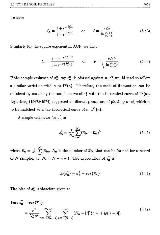
5.2. TYPE I SOIL PROFILES 5-34
we have
<5n -2A(
1 + e *
1 — e'2AI
66 =
2A /, ft” T 1 1 *„-l
(5.43)
Similarly for the square exponential ACF, we have
Sn =„( 42
1 + e ( s )
1 - e~6 =
\7tA/2
(5.44)
If the sample estimate of <r2, say s2, is plotted against n, s2 would tend to follow
a similar variation with n as T2(n). Therefore, the scale of fluctuation can be
obtained by matching the sample curve of s2 with the theoretical curve of T2(n).
Agterberg (1967&1974) suggested a different procedure of plotting n • s2 which is
to be matched with the theoretical curve of n • T2(n).
A simple estimator for <r2 is
= A yV,„ - <c„)27=i
(5.45)
Nnwhere /c„ = ^ Kin- Nn is the number of /ctn that can be formed for a record
i=iof N samples, i.e. Nn = N — n + 1. The expectation of s2 is
E{sl) =°n- var{Kn} (5.46)
The bias of s2 is therefore given as
bias s2 = var{icn}
—2 Nn-1 n — 1
W E E (lVB-|r|)(n-M)p(|r + .|)(5.47)
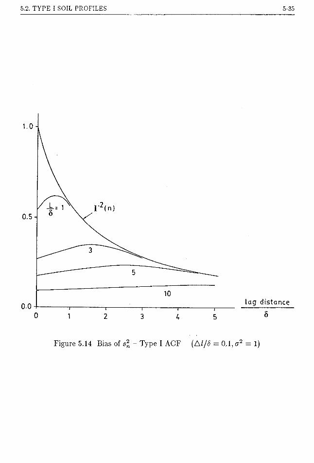
5.2. TYPE I SOIL PROFILES 5-35
Figure 5.14 Bias of - Type I ACF (A//<5 = 0.1, o2 = 1)

5.2. TYPE I SOIL PROFILES 5-36
Fig.5.14 shows the bias of the estimator s2 for a Type I ACF for the case
of A1/8 = 0.1 and a2 = 1. Also shown on the figure is the theoretical value of
r2(n). It can be seen that the bias is very substantial for a small sample size.
When the lag distance is larger than about half of the sampling length, the bias
is comparable to the theoretical value of T2(n) and therefore data points with lag
distances greater than this value should not be used for the estimation ACF. To
show the precision of the estimator s2, a more logical indicator would be the COV
defined in terms of the MSE, denoted as RCOV.
RCOVMSE of si
^/t>ar{s%} + {6ias sg}2(5.48)
The calculation of var{s„} is discussed in Appendix D. Fig.5.15 shows the plot
of RCOV for the same problem considered previously in Fig.5.14. The RCOV in
creases with lag distance indicating that the estimation s2 become more imprecise
as n increases.
Fig.5.16 shows the graph of T2(n) for the simple exponential ACF assuming
cr2 = 1. To use the graph, s2 has to be normalized by s2. In essence, r2(n) is
estimated by s2/s2. The value of A1/8 is read from the best fit curve and the
scale of fluctuation can be calculated accordingly.
Vanmarcke (1977c) suggested a simpler plotting procedure using the asymp
totic results of Eqn.5.42 for T2(n). Curves of 8n/n can be constructed for various
values of Sn. The value of Sn is determined from the curve which gives the best
fit to the data for large values of n. The scale of fluctuation can then be eval
uated accordingly using Equations 5.43 or 5.44 for examples. The procedure by
Vanmarcke (1977c) is simpler than the complete model, but suffers from the fol
lowing disadvantages. The value of s2 at large lag is more unreliable as indicated
in Fig.5.15. The information carried by the more reliable observations at smaller
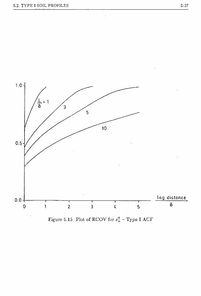
5.2. TYPE I SOIL PROFILES 5-37
Figure 5.15 Plot of RCOV for s“ - Type I ACF

5.2. TYPE 1 SOIL PROFILES 5-38
r2(n)
i Al
number
Figure 5.16 Plotting Graph for T2(n) - Type I ACF

5.2. TYPE I SOIL PROFILES 5-39
lag distances is wasted. Furthermore, the curvature of r2(n) is small at large lag.
Consequently, the data at large lag distances can normally be fitted equally with a
range of values of Sn and the determination of a suitable value for Sn becomes less
certain. All well-behaved ACFs have the same asymptotic equation as Eqn.5.42.
Unless an ACF can be chosen based on other considerations, the knowledge of 6n
does not enable the scale of fluctuation to be calculated.
With the availability of computer plotting facility, graphs can be easily con
structed for different ACFs with different parameter values. By this method, the
procedure using the complete model is as simple as the simplified procedure by
Vanmarcke (1977c), but more accurate.
The variance plot for data sets 1 and 3 are shown in Fig.5.16. It can be
seen that the autocorrelation structure of the cone resistance (data set 1) is well
described by a Type I ACF with A1/6 = 0.1, which in turn implies a value of
5 equal to 0.2m. This is in good agreement with the values obtained from other
methods discussed above. A value of Al/S = 0.4 gives the best fit to the third set
of data (although it is apparent that a Type I ACF does not give an exact fit).
This yields a scale of fluctuation of 12.5ft as compared to a value of 10ft obtained
from the simplified procedure by Vanmarcke (1977c) who also assumed a simple
exponential ACF for the soil property.
5.2.5.3 Curve fitting by least squares
Instead of fitting by ‘eye’, a more objective way for fitting a model to the
sample ACVF, ACF or variogram is by means of least squares. The least squares
method is often used purely as a numerical criterion for obtaining a good overall
fit to the experimental curve.
Suppose G(h\9), where 9 is the collection of parameters, is the curve to be
fitted to the experimental curve G(h\9). For instance, G(h\9) may be the ACVF
C(h) = p(y\c*) where a is the parameters of the ACF and 9 = (<r2,a). G(h\9}

5.2. TYPE I SOIL PROFILES 5-40
may be the estimator C\(h) for C(h). The parameters are obtained by minimizing
the sum of squares of the residuals, i.e.
min£yC7(Ai|£) -G(/i,|0)}2 (5.49)~ t
The use of the least squares method is to avoid the subjectivity inherent in the
procedure of curve fitting by ‘eye’. Sometimes, weights W{ are assigned to the
residuals to obtain a more reasonable criterion of curve fitting. The weighted least
squares procedure is described by
min Wi{G(hi\9_) — G(hl\9)}2 (5.50)— i
A larger weight is assigned to more reliable estimates and vice versa. Here the
choice of wt is also empirical. The program developed by Tough and Leyshon
(1985) is an example of this.
The least squares method can also be used as a statistical procedure for es
timating the parameters of the model, also called regression analysis. Neglecting
the biases of G(h\0). the following model may be used.
G(hi\0) =G(ht\6) + ei (5.51)
where et are the random errors with zero mean. The error term is related to the
random component (.(tj) of the soil property at the sample locations. As G(ht\0)
and G(hj\9) are estimated from the same set of observations, the error terms
et and e3 would also be correlated. The ordinary least squares method, which
assumes independence of error terms, is not appropriate for this case. Instead, the
generalized least squares (GLS) method should be used and the following problem
will have to be solved.
min|{G(/lt|£) - G(ht\0)}TVe~l {G(h,\0) -G(A,-|0)}} (5.52)

5.2. TYPE I SOIL PROFILES 5-41
where G(h{\9) = [G(hi |0), G(/i2|$), • • -]r and similarly for G(ht\9). Vg_ is the co
parameters. The solution for Eqn.5.52 is quite involved. To reduce the computing
effort, a weighted least squares method could be used in which the off-diagonal
Cressie (1985) seems to be the first to develop this approach to fitting a theoretical
model to the sample variogram and derived a series of formulae for the calculation
of Ve_ for the estimators 7i(^) and l3{h) (Equations 5.27 and 5.29). For model
fitting of ACVF, the covariance matrix of the error terms can be obtained using
Eqn.5.15.
Although the use of Equations 5.52 and 5.53 is more justifiable than Equations
5.49 and 5.50, the latter are often used for expediency.
5.2.6 Effects of regularization
The properties of a soil at a point are purely a mathematical abstraction.
In practice, soil properties can only be measured from a specimen with finite
dimensions. In geostatistics, the average property kv measured from a sample with
dimension v(£) centred at a point t is called the regularized property over a support
v(t). The same term is used herein for soil properties. Only one dimensional
regularized soil properties will be considered here, but the conclusions drawn from
the following discussion apply equally well to the case of two or three dimensional
regularized properties.
Consider a length of dimension / centred at a point t (Fig.5.17), the regularized
variance matrix of the error terms. Note that the matrix V0 1 also depends on the
terms of Ve 1 are neglected. As a result, Eqn.5.52 becomes
(5.53)
soil property is defined as

5.2. TYPE I SOIL PROFILES 5-42
K(t)
Figure 5.17 Regularization of Soil Property over a Length /
The ACVF Ci(v) of ki(t) can be defined as
Q(v) = cov{ki(t),ki(t + t>)} = a2 • B(l, /; v) (5.55)
where B(IJ; v) is the covariance factor of two line average each having an averaging
length of / and separated by a lag distance of v. As var{ki(t)} = a2 • r2(/), the
ACF pi(v) of ki(t) can be obtained as follows.
Pl{v) =-----TTBxvar{Ki(t)}
B(l,hv)F 2(/)
_ Jo(/ ~ t)(p(v + r) + p(v - T))dr
2 fo(l~ r)p(r)dr
(5.56)
Note Ci(v) and pi{v) are defined only for v > l.
Fig.5.18 shows the ACF of ki(t) for different supports v for a Type I ACF.
The ACF of ki{t) deviates from the point ACF as the ratio 1/6 increases. Note
that in Fig.5.18, b is assumed to be known. It is therefore not suitable as plotting
graph of the ACF to be used for the estimation of the ACF.
Define c to be the ratio of the length of the sample to the sampling interval,
i.e. c = l/Al. The correct plotting graph is shown in Fig.5.19 for the case of
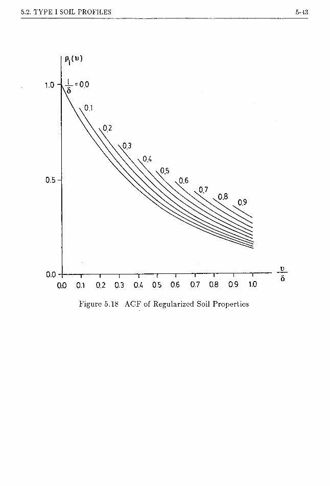
5.2. TYPE I SOIL PROFILES 5-43
0.2 0.3 0.4 05 0.6 0.7 0.8 0.9 1.00.0 0.1
Figure 5.18 ACF of Regularized Soil Properties

5.2. TYPE I SOIL PROFILES 5-44
A C F
c = 0.0
c = 0.5
\\N
\\\\ v\\\\V
number
Figure 5.19 Plotting graph for Regularized ACF
5.2. TYPE I SOIL PROFILES 5-45
c = 0.5 and a Type I ACF. The plotting graph for the point property (c = 0) is
also shown in the figure for comparison. Consider the extreme case of A1/6 = 0.5
which means that the support l is equal to one quarter of the scale of fluctuation.
As indicated in Fig.5.19, the difference between the two sets of curves is small
even though the length of the sample is relatively large as compared to the scale
of fluctuation in this case. Therefore, regularization of soil properties has little
influence on the estimation of the point ACF.
The effect of regularization on the a factor is examined next. For regularized
soil properties, the a factor should be calculated using the following equation (for
the one-dimensional case).
(5-57)t=ij—\
where cq is the a factor for regularized soil properties and vl3 is the lag distance
between sample points.
Fig.5.20 compares the a factors for point properties and regularized properties
for the case of c — 0.5. The a factors are so close for the cases of A1/6 = 0.05 and
0.2 that they cannot be distinguished in the figure. Even for the somewhat extreme
case of Al/8 = 1 in which the soil properties are regularized over a length equal
to half of the scale of fluctuation, the difference is still less than 10%. Therefore,
the effect of regularization on the ot factor can be ignored in practice.
However, regularization does have some influence on the estimation of the
point variance. The estimator s2 defined by Eqn.5.6 only gives the estimate of
the variance of the regularized property. To calculate the point variance, a further
correction for the variance reduction due to spatial averaging over the domain of
the support is required. Referring the Equations 5.4 to 5.6, the corrected point
variance estimator based on regularized properties should be

5.2. TYPE I SOIL PROFILES 5-46
a , a(
number of sample
Figure 5.20 a Factor for Regularized Soil Properties
5.2. TYPE I SOIL PROFILES 5-47
where sf is the variance estimate obtained from regularized samples using Eqn.5.4,
viz
= 0~«i)2 (5-59)i=i
If the sample size is relatively large in comparison with the scale of fluctuation,
the variance reduction due to regularization is significant. For instance, if 1/8 =
0.5, r2(/) becomes 0.74 for the Type I ACF. Therefore, the point variance will be
underestimated by 25% if the effect of regularization is not accounted for.
For a Type I soil profile, the mean value of regularized properties is the same as
that of the point properties. Therefore, the sample mean value of the regularized
properties 7q can be used directly as an estimator of the point mean value. In this
case, the trend variance becomes var{ki} instead of var{Jz} derived in Chapter 4
based on the sample point mean value 7c. Therefore
trend variance = t>ar{/q} = cq • var{ki(t)} (5.60)
where cq is given by Eqn.5.57 and var{ki(t)} can be estimated using a equation
similar to Eqn.5.6. Therefore,
vqt[ki} (5.61)
where sf is given by Eqn.5.59. Note there is no need to correct for the variance
reduction due to regularization for the trend variance. In fact, the larger the
support is, the smaller will be var{ki(t)} due to variance reduction and hence the
trend variance. This is one of the reasons why the testing of large block samples
in the field is usually considered to give a more accurate estimate of the strength
parameters than that obtained from small samples in the laboratory.
In summary, regularization has the following consequences on the structural
analysis of soil data.
5.3. TYPE II SOIL PROFILES 5-48
1. Regularization has little effect on the estimation of ACF. However, the sample
ACF at lag distances smaller than the dimensions of soil samples cannot be
obtained from regularized samples. If the scale of fluctuation is comparable to
the dimensions of the soil samples, details of the ACF at small lag distances
cannot be revealed. The estimate of the ACF will invariably be crude in this
case. However, it is not considered to be a handicap. In practice, the dimen
sions of soil samples are usually small, of the order of 10cm or less. If the
scales of fluctuation are comparable to the dimensions of the samples, it would
necessarily mean that the scales of fluctuation are also small. In this case, the
variance reduction due to spatial averaging in a slope would be so significant
that total uncertainty will be dominated by other factors such as the trend
variance rather than the spatial variability of soil properties, and an accurate
estimation of the scale of fluctuation becomes unimportant.
2. The influence of regularization on the a factor is small. In practice, the a
factor based on point properties can be used even for regularized properties.
3. The variance of regularized properties is smaller than that of the point prop
erties. The estimating the point variance by the variance of the regularized
properties will lead to unconservative results. However, this effect can be ac
counted for easily using Eqn.5.57.
4. Regularization has the effect of reducing the trend variance. Therefore, estima
tion of mean soil properties based on larger specimens is more accurate than
that on small specimens.
5.3 TYPE II SOIL PROFILES
5.3.1 Introduction
For a Type II soil profile, the trend component as well as the correlation

5.3. TYPE II SOIL PROFILES 5-49
structure of the random component have to be estimated. The structural analysis
of a Type II soil profile is complicated by the fact that:
• If the correlation structure is known, the trend component can be estimated
efficiently (in the statistical sense) using the generalized least squares (GLS)
method. However, if the correlation structure is not known a-priori, the proce
dure of GLS cannot be carried out. Although the ordinary least squares (OLS)
method can be used and produces the same asymptotic efficiency as the GLS
method (Priestley, 1981), the method will be less efficient for small samples
and always underestimates the variance of the trend component.
• If the trend component is known a-priori, the random component of the sample
can be obtained simply by subtracting the trend value from the observed value
and the procedure for estimation of the correlation structure becomes identical
to that of Type I soil profiles. If the trend is not known a-priori, the correlation
structure of the random component may be estimated from the residuals of the
fitted trend, via £; = K(t{) — g(tt). However, such a procedure will produce
highly biased results and the resulting correlogram or variogram may bear
little resemblance to the true situation (Matheron, 1971; Johnston, 1972).
The difficulty now becomes clear; the trend component cannot be estimated
efficiently without the knowledge of the correlation structure of the random compo
nent and the correlation structure cannot be established without some knowledge
of the trend component.
In the following, a simplified procedure of structural analysis of soil data
for Type II soil profiles is introduced, followed by the discussion of an iterative
least squares method and the maximum likelihood method for the simultaneous
estimation of the trend component and the random component. The techniques
by Matheron (1973) and Delfiner (1976) for filtering out the trend component will
also be mentioned.

5.3. TYPE II SOIL PROFILES 5-50
5.3.2 A simplified procedure
If the soil property has no horizontal trend, the following procedure may be
used.
Figure 5.21 Sample Locations in a Soil Profile
The principles can be illustrated using the simple example in Fig.5.21. Sup
pose soil measurements are made on samples taken from boreholes A and B at
the locations indicated in the figure. The arrows shows the scales of fluctuations
of soil properties based on the prior knowledge. One way to minimize the corre
lation between the samples is to use only the test results for borehole A having
a separation distance greater than 6y for the estimation of the trend component
for instance the test results at Ai, A^, Ay etc. The test results so obtained will
be largely independent and the trend component can therefore be estimated using

5.3. TYPE II SOIL PROFILES 5-51
the ordinary method of least squares.
Residuals are then calculated by subtracting the estimated trend component
from the test results. The structural analysis of residuals would then be the same
as a Type I soil profile. Data from other boleholes can also be aggregated to obtain
a more accurate estimate of the trend component. For instance, test results with
separation distance greater than 6y are chosen from borehole B (e.g. at locations
Bi, B4, B7 etc). As boreholes A and B are separated by a distance greater than 6X,
the test results obtained from the two boreholes can be regarded as independent
of each other. Consequently, all the test results from Ai, A4, A7,...and Bi, B4,
B7,.. .can be lumped together from which the trend component can be estimated
using the ordinary method of least squares.
The above procedure breaks the circularity discussed above, but at the expense
of wasting some of the information carried by the test results which have not been
chosed for the estimation of the trend component.
5.3.3 Iterative least squares method
As mentioned earlier, the difficulty in analyzing a Type II soil profile arises
from the fact that the estimation of the trend component requires the knowledge
of the correlation structure and vice versa. This circularity may be broken by an
iterative least squares method as suggested among others by Johnston (1972), Ord
(1975), Sabourin (1976), Ripley (1979) and Bennet (1979).
Firstly, the trend component can be assessed using the generalized least
squares method and a reasonable ACF for the random component. The ACF is
then estimated from the residuals obtained from the fitted trend. With the newly
estimated ACF, the trend component is then re-calculated using the GLS method.
The process is repeated until (hopefully) the changes in the trend component and
the ACF are small.
There is no common consensus as to how the iterative least squares method

5.3. TYPE II SOIL PROFILES 5-52
should be implemented. The following criterion based on the GLS method is
proposed herein. The criterion can be stated as
min J(0) = min eT A le e_ e_
(5.62)
where e = [fi, €2, • • •, £n]T denotes the realized random components of the soil
samples, given by
(, = «(<,) - g(ii) = KiU) - ^2 aj PjiU) (5.63)3
and A is the theoretical autocorrelation matrix (AM) of e. Under the assumption
of stationarity, the AM has the form
r 1 P12
1
A(a) = Sym
P13 Pin
P23 ••• P2N
1 * • • P3N >
1
(5.64)
where pij is the autocorrelation between sample i and j described by the ACF
p(i;|a) with parameters a. 0 is the parameter vector comprised of the trend coef
ficients a and the parameter a of the AM. Note that t{ does not have to follow a
regular pattern in space.
If the AM is given a-priori, the estimate of the coefficient of the trend compo
nent given by the solution of Eqn.5.62 is BLUE (best linear unbiased estimator,
see e.g. Kendall and Stuart, 1961). Furthermore, the least squares estimate of the
trend coefficients are given by (Draper and Smith, 1981)
2= (PtA-1P)-1PtA~1k (5.65)
1s = (a - P a)T A l(tz -Pa)N-k (5.66)

5.3. TYPE II SOIL PROFILES 5-53
where N and k are respectively the number of samples and the number of terms in
the generalized polynomial (Eqn.4.5). a is a k x 1 column vector representing the
coefficients of the generalized polynomial, k is the vector of measured soil property
at the N sample locations. P_ = (Fj, jP2,... ,P.^)T is a N x k matrix where P_t is
a A: x 1 vector representing the values of the variable of the generalized polynomial
at the ith sample location and the arrow means ‘estimated by’. The covariance
matrix V± is estimated by
Va -* s2(XTA~lX)-' (5.67)
If A(o) is not known a-priori, the parameter 6 has to be optimized to give the
minimum value of J{9). It is easily proved that
min J(9) = min J(9) t 2.-a
mina
mina •J(fi)]
min[/F(a)]a
(5.68)
Eqn.5.68 can be interpreted as an iterative least squares procedure. Given the
value of a (i.e. the ACF is prescribed), the trend component is estimated using
the GLS procedure. The parameter a is then adjusted until the change of H(a)
and hence the trend component is small. Note that when a is specified, say Oy,
the function Ff(ay) is simply the solution of the GLS given A(a) — A(ft;) and
the solution for a and cr2 is given by Equations 5.65 to 5.67. In fact, Ff(oy) can
be solved readily by available statistical computing package, such as the IMSL
packages (IMSL, 1984). Therefore, the optimization problem of Eqn.5.68 is now
reduced to a much simpler problem of optimization H(a) with respect to a. In
particular, if a contains only one parameter, Eqn.5.68 can be solved efficiently
using the technique of rational approximation (see Appendix E). If a has more
than one variable, the problem may be solved by the optimization technique for
5.3. TYPE II SOIL PROFILES 5-54
multivariate functions outlined in Appendix F. Other optimization techniques can
be found in Jacoby et a1 (1972).
Different ACFs or generalized polynomials may be used. The model which
gives the smallest value of J(6) can be regarded as the most suitable model.
Although the legitimacy of the iterative least squares procedure does not seem
to have been proven in any general manner, the method is commonly used for
expediency and as a compromise between theory and practice. A recent example
of the application of the iterative least squares procedure is given by Sadeghipour
and Yeh (1984) for the estimation of the transmisivity of a homogeneous aquifier.
It must be noted that the iterative least squares method does not guarantee
a feasible estimate for the parameters. To tackle this problem, Eqn.5.68 has to be
converted into a constrained optimization problem in which the parameters are
restricted to within their feasible ranges as is done in Sadeghipour and Yeh (1984).
5.3.4 Maximum likelihood estimation
If the joint distribution of the soil property is known, the parameters of the
model can be estimated using the method of maximum likelihoods (ML). In prac
tice, the joint distribution of soil properties is not known. A joint Gaussian distri
bution is usually assumed partly because the marginal distribution (which is also
the point distribution) can usually be approximated by a Gaussian distribution
with reasonable accuracy (e.g. Lumb, 1966; Matsuo, 1976), but mostly because of
convenience. The use of a joint Gaussian distribution is analogous to the use of
linear elasticity theory in settlement analysis. The assumption is not strictly cor
rect but often gives reasonable results in practice. The method of ML is discussed
in most references on statistics such as Cremer (1946); Arnold (1981) and Mood
et al (1974). If a Gaussian distribution is assumed for the random component of

5.3. TYPE II SOIL PROFILES 5-55
the soil property, the likelihood function is given by
m(27TCT2) T
exp(-^iT^ li) (5.69)
The same notation of Eqn.5.62 is used in Eqn.5.69 and \A\ is the determinant of
the autocorrelation matrix.
Maximizing the likelihood function with respect to the parameters 0 is equiv
alent to maximizing the log-likelihood function M — In L(0).
M — — — In 27r — — In a2 — - In \A\-------eT A~ls (5.70)2 2 2 2 (j
The ML estimate of the point variance g2 is given by
a2 eTA~lsN (5.71)
Substituting Eqn.5.71 into Eqn.5.69, we have
M = -y (1 + In 2w — Id N) — j 7(5)1 (5.72)
where J(6) is defined in Eqn.5.62. Thus, maximizing the log-likelihood function
is equivalent to the minimization of the following function
Q(i) = min|yl| *./(£) (5.73)0_
Note if A = I, the identity matrix (which also means that the random component
is an uncorrelated process), the GLS procedure and the ML estimation are iden
tical. can be treated as a weighting function and the ML estimation can be
interpreted as a ‘weighted’ GLS procedure. Compare the weighting function \A\k
for a time series and a spatial series. For a first order autoregressive model AR(1),
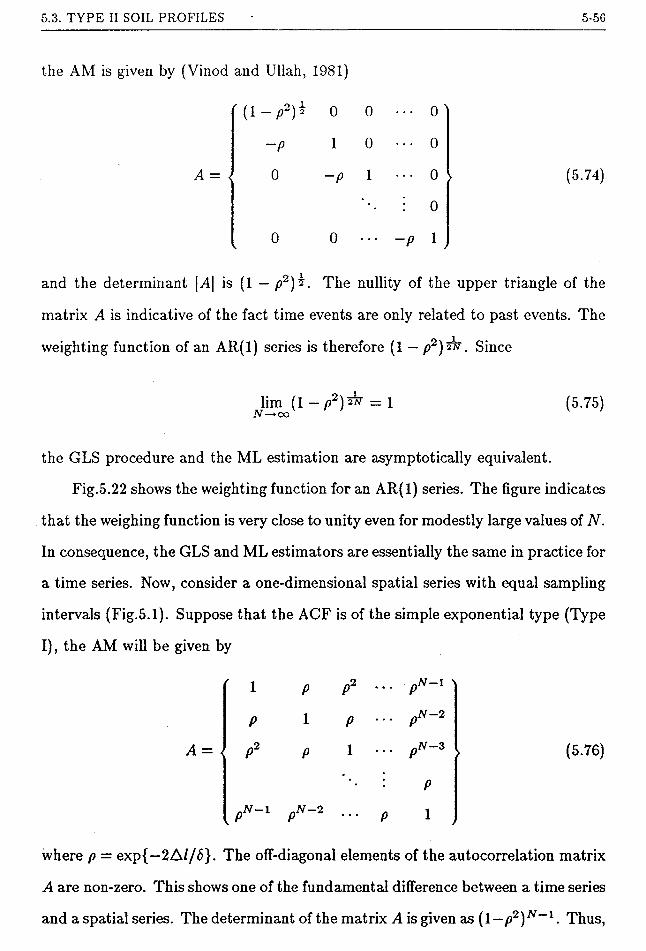
5.3. TYPE II SOIL PROFILES 5-56
the AM is given by (Vinocl and Ullah, 1981)
'(1 -p2)* 0 0 O'
~P 1 0 ••• 0
A = 0 -p 1 0 (5.74)
0
0 0 ••• -p 1
and the determinant \A\ is (1 — p2)?. The nullity of the upper triangle of the
matrix A is indicative of the fact time events are only related to past events. The
the GLS procedure and the ML estimation are asymptotically equivalent.
Fig.5.22 shows the weighting function for an AR(1) series. The figure indicates
that the weighing function is very close to unity even for modestly large values of N.
In consequence, the GLS and ML estimators are essentially the same in practice for
a time series. Now, consider a one-dimensional spatial series with equal sampling
intervals (Fig.5.1). Suppose that the ACF is of the simple exponential type (Type
I), the AM will be given by
weighting function of an AR(1) series is therefore (1 — p2)™ . Since
lim (1 — p2) 2^ = 1 (5.75)
1
P
A= P2 P (5.76)
P
P 1
where p = exp{—2A//<5}. The off-diagonal elements of the autocorrelation matrix
A are non-zero. This shows one of the fundamental difference between a time series
and a spatial series. The determinant of the matrix A is given as (1— p2)N~l. Thus,

5.3. TYPE II SOIL PROFILES 5-57
time series
spatialseries
0.0 0.1 0.2 03 0.4 0.5 0.6 07 0.8 09 1.0
Figure 5.22 Weighting Function for ML Estimation
the weighting function becomes (1 — p2)~Fr~. As n oo, the weighting function
approaches the limiting value of (1 — p2). Fig.5.22 also shows the variation of the
weighting function for the spatial series. The variation of the weighing function is
for the spatial series much more pronounced than that of the AR(1) time series. As
a result, a larger difference between the GLS and ML estimates of the parameters
for the spatial series would be expected. The GLS procedure would yield a larger
value of p and hence a larger scale of fluctuation than the ML procedure.
Which method is better, the GLS procedure or the ML estimation, is debat
able. The influence of the choice of the GLS or ML estimates on the final predicted
value of failure probability of slopes remains a question of further inquiry. For ex-

5.3. TYPE II SOIL PROFILES 5-58
ample, although the GLS procedure gives a larger value of the scale of fluctuation
6 which also means that the predicted value of the variance reduction due to spa
tial averaging is smaller, a larger value of 6 will also imply a smaller predicted
variance for the coefficient of the trend component and hence a smaller predicted
trend variance. Further investigation needs to be done to establish whether the
failure probability of slopes based on the GLS procedure is greater or smaller than
that based on the ML estimation.
Given the value of a, say the ML solution under the assumption of a joint
Gaussian distribution is the same as that obtained using the GLS procedure and
hence the conditional estimates of the parameters are also given by Equations 5.65
to 5.67. Using the same argument as in Eqn.5.68, the MLE can be re-formulated
as
min Q(([) = min6_ a
I A\*H(a) (5.77)
where H(a) is defined by Eqn.5.68. Eqn.5.77 can be solved using the same tech
nique as discussed previously for the GLS procedure.
Again different ACFs and generalized polynomials may be used. The most
suitable model can be identified using the Minimum Akaike’s Information Criteria
as suggested in Matsuo and Asaoka (1977).
It is well known that the maximum likelihood estimation yield asymptotically
efficient estimates for independent identically distributed samples (see Cremer,
1946, pp500-504). For spatial data, the observations are autocorrelated among
themselves. Intuitively, the same property should also hold for spatial data as N
becomes large provided that the an increase in N is accompanied by a simultaneous
increase in the sampling domain. The problem has been recognized by statistician
(e.g. Arnold, 1981), but a formal proof is not yet available to the knowledge of the
Author.

5.3. TYPE II SOIL PROFILES 5-59
Once the optimum value of a is ascertained using Eqn.5.77, the estimates of
the coefficients of the generalized polynomial and its covariance matrix can be ob
tained using Eqn.5.65 and Eqn.5.67 except that the parameter a is replaced by the
ML estimate and the s2 is given by Eqn.5.71. Alternatively, the covariance ma
trix of the parameters can be approximated by the inverse of Fisher’s information
matrix M, i.e. Vg = M~l and the entry of the matrix M is given by
r _ ^ In L(0)~ aq an. (5.78|
where 9t is the element of 6 and the derivative is evaluated at the ML estimates.
The exact evaluation of Eqn.5.78 would be very involved. Alternatively, the deriva
tives can be calculated numerically using the technique of rational extrapolation
(Li and White, 1987d). One advantage of using ML estimation is that estimates
of the sampling variance of a can also be obtained using Eqn.5.78. Note that the
ML estimation normally gives biased estimates of the parameters. However, the
bias should be small if N is large.
5.3.5 Filtering out of the trend component
The approach of filtering out the trend component is first proposed by Math-
eron (1973) and later elaborated by Delfiner (1976). However, active research on
this approach only started in the 1980s and a series of paper on the subject has
appeared over the past few years. The approach is still in a state of develop
ment. The drawbacks of the original proposal by Delfiner (1976) are pointed out
by Starks and Fang (1982) and also discussed in Kitanidis (1983). The approach
is later modified by Kitanidis (1983&;1985), Marshall and Mardia (1985) and Stein
(1986).
The technique is discussed in detail in Delfiner (1976), Kitanidis (1983) and
Starks and Fang (1982). The following only briefly outlines the basic principles of
the method. Define a new random variable zi, called the increment, as a combi-
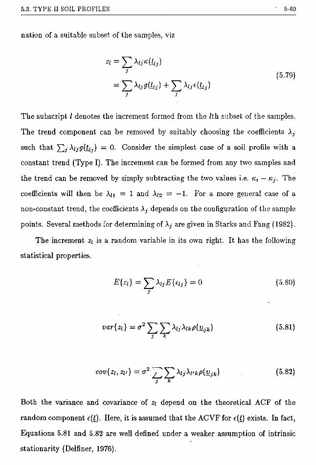
5.3. TYPE II SOIL PROFILES 5-60
nation of a suitable subset of the samples, viz
zi = ]Tp/yK%)(5.79)
= +yt ^h€(kj)j j
The subscript l denotes the increment formed from the /th subset of the samples.
The trend component can be removed by suitably choosing the coefficients Ay
such that = 0- Consider the simplest case of a soil profile with a
constant trend (Type I). The increment can be formed from any two samples and
the trend can be removed by simply subtracting the two values i.e. /ct — ACy. The
coefficients will then be Xu = 1 and A/2 = —1. For a more general case of a
non-constant trend, the coefficients A; depends on the configuration of the sample
points. Several methods for determining of Ay are given in Starks and Fang (1982).
The increment zi is a random variable in its own right. It has the following
statistical properties.
E{zl} = J^XljE{elj}=0 (5.80)
var{zi} = a2Y^^\ij\lkp(vjk) (5.81)
cov{zi,zi>} = a2 V]y" kjh'kp(vjk) (5.82)o k
Both the variance and covariance of zi depend on the theoretical ACF of the
random component e(t). Here, it is assumed that the ACVF for e(Q exists. In fact,
Equations 5.81 and 5.82 are well defined under a weaker assumption of intrinsic
stationarity (Delfiner, 1976).

5.4. TYPE III SOIL PROFILES 5-61
Delfiner (1976) suggested that the parameter 0 can be estimated using the
weighted least squares method. The criterion of estimation is
where wi is the weight assigned to the residuals and E{zf\9} is given by Eqn.5.81.
Note that the method of least squares is used only as a numerical criterion for
obtaining the estimate of the parameters. Other statistical procedure such as the
maximum likelihood estimation, the minimum unbiased quadratic estimation, the
minimum norm estimation and the modified norm quadratic estimation are also
used in the literature (Kitanidis, 1983&T985; Stein, 1986).
Once the parameters of the ACF is obtained, the coefficients of the trend
component and the point variance can be estimated using the GLS procedure as
if the ACF is known.
5.4 TYPE III SOIL PROFILES
The structural analysis of a Type III soil profile is the most complicated among
the three types of profiles. Literature on this subject is scarce. Asaoka and Grivas
(1982) presented a structural analysis of the undrained cohesive strength of a Type
III soil profile. However, it was assumed that the COV of cohesive strength Su
is directly proportional to the depth y (i.e. the trend is assumed to be known) so
that the normalized strength Su/y could be modelled as a homogeneous random
field. Therefore, the analysis is more like a structural analysis of a Type I profile
than that of a Type III profile.
The difficulty of analyzing a Type III profile lies in the fact that the random
component is also related to the trend component. Even if the trend component
can be filtered out using the procedure in Section 5.3.3, the dependence of the
mine_ (5.83)

5.4. TYPE III SOIL PROFILES 5-62
random component on the trend component still exists and no suitable procedure is
yet available for filtering out such a dependence. Consequently, the GLS procedure
and the ML estimation discussed previously for Type II soil profiles seems to be
the only two options that can be extended to the structural analysis of Type III
soil profiles.
For Type III soil profiles, the GLS procedure will lead to an equation similar
to Eqn.5.62, but according to Eqn.4.11c, the element atJ of the AM would become
= g(Li) • g(Lj) • Pij (5-84)
Eqn.5.73 has to be modified in a similar manner for Type III soil profiles. Since the
covariance matrix also contains the coefficient of the trend component, Equations
5.68 and 5.77 are not valid for Type III soil profiles. The functions J(9) and Q(0)
have to be optimized using multivariate optimization techniques.
Equations 5.65 to 5.67 are not valid for the calculation of the trend component.
No suitable procedure is yet available for estimating the covariance matrix of
the trend coefficients for the GLS procedure. However, Eqn.5.78 remains a valid
approximation for the covariance matrix using the ML estimation.
A review of the current literature indicates that a Type III soil profile is
usually associated with the undrained cohesive strength of clays. Following a
similar procedure as in Lambe and Whitman (1969), the undrained shear strength
can be related to the effective strength parameters as follows:
\K0 + (1 — K0)Af \ sin (f)'a'y + c‘ cos (f)' u [1 + sin <f>'(2Af — 1)]
where
K0 = coefficient of earth pressure at rest
Af — pore pressure coefficient at failure

5.5. PLANNING OF A SITE INVESTIGATION 5-63
c' — effective cohesion
(f)' — effective angle of shearing resistance
Gy — overburden pressure
The overburden pressure is given by 7y • y where 7y is the average soil density over
a depth y. For normally consolidated clays, c' is small so that Eqn.5.85 becomes
Su = ? * 7y • V ' (5.86)
where f = [K0 + (1 — /60) Ay] sin 0'<ry/[l + shuf),(2Af — 1)]. If K0, A/ and </>'
have constant statistical properties within the soil profile, Su will appear like a
Type III soil profile with a linear trend and a constant COY. Therefore, a Type
III soil profile for the undrained shear strength may very well be a Type I soil
profile in terms of the effective soil parameters. If it is the case, the question arises
of whether it would be more cost effective to determine the statistical properties
of the undrained shear strength from direct measurements or indirectly through
the measurements of the effective soil properties. The cost effectiveness may be
measured in terms of the number of soil samples required and the total cost of soil
testing involved to achieve the same predicted value of failure probability. This
question remains unresolved at this stage.
5.5 PLANNING OF A SITE INVESTIGATION
The basic procedure of structural analysis of soil data has been discussed
above. This section summarizes some of the guidelines for planning a site investi
gation.
To design a slope to a specified failure probability, it is necessary to know
the mean value, the point variance and the ACF of soil properties. As discussed

5.5. PLANNING OF A SITE INVESTIGATION 5-64
earlier in Chapter 4, the magnitude of variance reduction due to spatial averaging
depends largely on the ratio of the scale of fluctuation to the dimension of the
slope.
In a preliminary site investigation, soil properties can be measured at close
spacings using some inexpensive tests such as the CPT or index tests. Techniques
for obtaining the scale of fluctuation were discussed in Sections 5.2.4 and 5.3.3.
If the results indicate a small scale of fluctuation in comparison to the di
mension of the slope, the variance reduction would be appreciable. The total
uncertainty will then be dominated by the uncertainty in the estimation of the
trend component. In this case, further tests to obtain a more accurate estimate
of the ACF are of little value. Instead, emphasis should be put on the estima
tion of the trend component so as to reduce the variance of the sample spatial
average, which is roughly proportional to l/N for Type I soil profiles when the
variance reduction factor is small. To maximize the effectiveness of soil sampling,
samples should be taken at spacings greater than at least one scale of fluctuation
so as to minimize the correlation. The trend component can then be estimated
using the procedure discussed above in this Chapter (e.g. Section 5.2 for Type
I soil profiles). As the samples are sufficiently far apart, the structural analysis
would be very simple. For instance, for a Type I soil profile, the point variance
and trend variance can be estimated using the usual estimators for independent
samples (Equations 4.58 and 4.59).
However, if the scale of fluctuation is large in comparison to the dimension
of the slope, the total uncertainty will tend to be significantly influenced by the
spatial variability of the soil properties. An accurate estimate of the ACF will
therefore be necessary so as to give a more precise calculation of the variance and
covariance of the spatial averages. As the scale of fluctuation is large, it may
not be feasible to take samples at wide enough spacings. Therefore, the effect of

5.5. PLANNING OF A SITE INVESTIGATION 5-65
correlation between the samples has to be accounted for in the calculation of the
a factor and the point variance (see e.g. Sections 5.2.2 and 5.2.3)
The strategy for a site investigation is different for analyzing the stability of
an existing slope for which some prior knowledge of the statistical parameters is
available. Soil samples may be taken at wide spacings to determine the mean soil
properties required for the analysis. The failure probability can then be estimated
using the measured mean soil properties and some tentative values of COV or 8
based on the prior knowledge. If the failure probability is sufficiently small, there
will be no need for further data collection. However, if the preliminary analysis
indicates a high value of failure probability, a more precise analysis or a re-design
of the slope may have to be considered. The planning of the site investigation
would then be the same as that discussed above for the design of slopes.

CHAPTER 6
PROBABILISTIC DESIGN OF SLOPES
6.1 INTRODUCTION
Over the past decade or so, there is a trend towards use of a probabilistic
approach for assessing the safety of slopes. Some elementary analyses based on
FOSM approach have already appeared in some textbooks in geotechnical engi
neering (e.g. Harr, 1977; He and Wei, 1979; Lee et a/, 1983). There is little doubt
that the more rational probabilistic approach will become more popular in the
future.
The literature on probabilistic analysis of slopes is now very extensive. How
ever, many of the these papers have fallacies in one way or the other and therefore
care must be taken not to be confused or misled when reading references on this
subject.
This Chapter therefore attempts to outline the historical development of prob
abilistic slope design and more importantly gives a critical discussion on some of
the shortcomings of existing approaches. The discussion is then followed by the
presentation of three probabilistic approaches of slope design. Examples are also
given to illustrate the implementation of these approaches.
6-1

6.2. HISTORICAL DEVELOPMENT 6-2
6.2 HISTORICAL DEVELOPMENT
The application of statistics to soil mechanics was pioneered by Lumb (1966,
1967,1968,1970) in the sixties whose work concentrated on the statistical descrip
tions and modelling of the stochastic nature of soil properties.
Wu and Kraft (1970) appears to be one of the earliest attempts at probabilis
tic analysis of slopes, but only a <f> = 0 analysis was considered. The performance
function of a slope was formulated perhaps for the first time as a safety margin.
They also recognized the importance of spatial variability and the sampling un
certainty of soil properties, and considered the model uncertainty in the analysis.
Although the analysis presented by Wu and Kraft (1970) is somewhat rudimentary
in the light of present-day development, it has all the ingredients of a ‘modern’
analysis.
Cornell (1971) also presented a probabilistic analysis for 0 — 0 slopes in
which he made two major contributions. Cornell was the first to point out the
relevance of autocorrelation of soil properties in a slope design and proposed a
stationary spatial process for its modelling. He also elucidated the concept of
system reliability in slope design and pointed out that a slope should be treated
as a system in series with the failure probability for the most critical slip surface
serving as the lower bound of the system failure probability. The notion of spatial
autocorrelation was later treated in greater detail by Lumb (1974& 1975a).
The work of Wu and Kraft (1970) and Cornell (1971) was later extended by
Yucemen et a/ (1973) to cover c-0 slopes using the ordinary method of slices as
the stability model.
Following up the work by Cornell (1971), his student Morla Catalan (1974)
performed a few analyses on the system reliability of slopes for 0 = 0 slopes
and came up with the tentative conclusions that the system failure probability is
substantially greater than the lower bound value given by the failure probability

6.3. REVIEW ON EXISTING APPROACHES 6-3
for the most critical slip surface.
Another milestones in probabilistic design of slopes is the work by Alonso
(1976) which forms the basis of many of the later studies. In his work, a more ac
curate simplified Bishop’s method was used for the formulation of the performance
function and more rigorous treatments of the autocorrelation of soil properties wTere
introduced.
However, the most comprehensive treatment of spatial autocorrelation of soil
properties was given by Vanmarcke (1977a) who developed what is now commonly
known as the random field model. The random field model is now more or less a
standard tool for probabilistic modelling of soil profiles. Vanmarcke (1977b) also
presented the first three dimensional analysis of (f> — 0 slopes using a level crossing
approach.
After about a decade of cultivation, probabilistic geotechnical design has be
come a popular research topic since the mid-seventies and numerous papers has
appeared in various international journals and conference proceedings. However,
many of these later analyses have not progressed beyond the level of Alonso (1976)
and some of them may even lag behind those of Wu and Kraft (1970), Cornell
(1971) and Yucemen et a1 (1973).
However, a recent study by Luckman (1987) needs special mention here. In ad
dition to the conventional /^-approach commonly used in the literature, Luckman
(1987) has also used two other techniques for analysis, namely the /?///,-approach
and the first-order-marginal-distribution (FOMD) approach. He also used a rig
orous stability model by Spencer (1967) for the formulation of the performance
function. Further comments on Luckman’s work will be given later in Section 6.3.

6.3. REVIEW ON EXISTING APPROACHES 6-4
6.3 REVIEW ON EXISTING APPROACHES
The following is a review of some of the aspects of the current probabilistic
approaches to slope design. Comments on some other aspects will also be men
tioned where appropriate in later discussions. Most of the current approaches have
one or more than one of the following characteristics:
(1) The performance function G(2Q is typically formulated as
researchers (e.g. Wu and Kraft, 1970; Li and Lumb, 1987; Li and White,
1987b&e) used the safety margin
The popularity of Eqn.6.1 is understandable as it is more in line with the con
ventional concept of factor of safety. However, Eqn.6.2 is preferred to Eqn.6.1
for reasons to be discussed later in Section 6.4.
(2) The performance function is currently based on simplified stability models such
as the friction-circle method, the ordinary method of slices, simplified Janbu’s
method or simplified Bishop’s method. The use of simplified models reduces
the computational effort and more importantly enable the derivatives of the
performance function required in a FOSM analysis to be evaluated analyti
cally. However, it is at the expense of having a less accurate stability model.
In the past, the use of a rigorous stability model was hampered by the fact
that conventional solution schemes cannot provide an explicit definition for the
performance function. The interslice forces have to be obtained by iteration. In
consequence, the derivatives of the performance function had to be evaluated
- 1 = F-1 (6.1)
where F is the ratio of total resisting force to total disturbing force. Some
G(X) = R(X) - 5(X) (6.2)
6.3. REVIEW ON EXISTING APPROACHES 6-5
numerically by finite difference approximation as is done in Luckman (1987)
when using Spencer’s (1967) method. This problem is now' tackled by means
of the unified solution scheme outlined in Chapter 3.
(3) Although the importance of autocorrelation of soil property was pointed out in
the early 1970’s by Cornell (1971), explained more fully in Lumb (1974&1975a)
and emphasised time and again in more recent papers by Alonso (1976), Van-
marcke (1977a&;1980) and Castillo and Alonso (1985), papers which assume
perfect correlation of soil properties, either knowingly or not recognizing the
relevance of autocorrelation, still appear in various international journals or
conferences. As remarked by Baecher et a1 (1984), these analyses w'ould give
engineers the impression that probabilistic slope analysis have not progressed
beyond the level of those in early seventies.
As indicated in Fig.6.1 the failure probability under the assumption of perfectly
correlation is exceedingly high, of the order of 0.1-0.2, for the typical range of
design factor of safety of 1.2-1.4.
In the present w'ork, the autocorrelation of soil properties is properly considered
in the analysis by using the random field model discussed in Chapter 4.
(4) Current probabilistic analysis are usually based on the FOSM approach and
the reliability index (3 is used to measure the safety of slopes. As discussed
earlier in Chapter 2, the reliability index (3 is a ‘variant’ risk measure. Because
of this, some researchers suggested the use of Hasofer and Lind’s reliability
index (3hl in lieu of the conventional Cornell’s reliability index (3 (e.g. Nguyen,
1985c; Li and Lumb, 1987; Li and White, 1987bAe; Luckman, 1987).
Both the /^-approach and the (3hl-approach are used in the present work and
comparisons will also be made between the two reliability indices.
Since the joint probability distribution of soil properties is generally not known,
a Level III analysis is seldom performed in slope stability problems. Even if
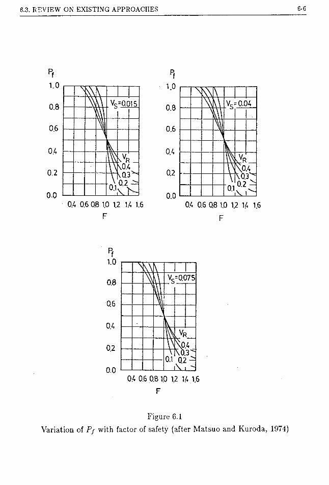
6.3. REVIEW ON EXISTING APPROACHES 6-6
S R _
0.2 — 0.2 -
0.4 0.6 0.8 1.0 1.2 1.4 1.6 0.4 0.6 Q8 1.0 1.2 1.4 16
F F
0.4 0.6 0.8 1.0 1.2 14 1.6
F
Figure 6.1
Variation of Pj with factor of safety (after Matsuo and Kuroda, 1974)

6.3. REVIEW ON EXISTING APPROACHES 6-7
the assumption of joint Gaussian distribution is used, the large dimension of
the problem would render such an analysis impracticable.
Nevertheless, a number of Level III analyses did appear in the literature. Mat
suo and Suzuki (1983) presented a Level III analysis for 0 = 0 slopes. In their
analysis, the soil density is treated as deterministic and they are therefore left
with only two random variables, namely the average cohesive strength over the
length of the slip surface which can be regarded as a Gaussian variate and the
model error which is considered to be uniformly distributed. The simplicity of
the performance function also enables the integrations to be performed without
much difficulty.
A number of Level III analyses for c-(j> slopes can also be found in the liter
ature. In these analyses, the failure probability is calculated either by direct
integration (e.g. Tobutt and Richards, 1979) or Monte Carlo simulation tech
niques (e.g. Tobutt, 1982; McPhail and Fourie, 1980; Prist and Brown, 1983;
Ramachandran and Hosking, 1985; Nguyen and Chowdhury, 1984). However,
these analyses are made possible by the incorrect assumptions that soil prop
erties are perfectly correlated so that they can be modelled as simple random
variables. Under this assumption, the cohesion for example for the entire slope
is treated as one simple random variable instead of n random variables (the n
values of average cohesion for all the n slices) for the random field model. Thus,
the total number of random variables can be limited to a few and consequently
a Level III analysis, although time consuming, may still be tractable. These
analyses, however complicated or rigorous they may seem, grossly overestimate
the failure probability giving no real indication of the safety of slopes.
Some approximate Level III analyses based on the advanced-first-order-second-
moment (AFOSM) method have also been proposed. Ramachandran and Hosk-
ing (1985) used the technique of Normal tail approximation developed by Rack-

6.3. REVIEW ON EXISTING APPROACHES 6-8
witz and Fiessler (1978). However, the assumption of perfect correlation was
used in their analysis.
Luckman (1987) used the so-called first-order-marginal-distribution (FOMD)
method developed by Der Kiureghian and Liu (1986). This may be regarded as
the first approximate Level III analysis for c-(p slopes to date (other approaches
in the literature are not exactly a Level III analysis for reasons discussed above).
The basic principle is as follows. Given the marginal distributions and co-
variances (or coefficients of correlation) of the random variables, whether it
be simple random variables or spatial variables, a joint Gaussian distribution
can be fitted to the random variables using the procedure developed by Der
Kiureghian and Liu (1986). Having obtained the fitted joint Gaussian distri
bution, the procedure for determining the reliability index is similarly to that
of a Level II analysis. Of course, the two central questions to be answered are
how to determine (a) the marginal distributions and (b) the covariances of the
random variables, especially the spatial random variables.
To answer the first question, Luckman (1987) assumed that the marginal distri
butions of the spatial random variables were the same as their respective point
distributions, the implication being that spatial random variables (e.g. c[) were
perfectly correlated within the domain under consideration, typically the di
mension of a slice. This assumption has two shortcomings. Firstly, for this
assumption to be justified, the averaging dimension must be small compared
to the scale of fluctuation. For a typical slope stability analysis, it would often
imply a large number of slices of the order of 102. Secondly, even if the assump
tion of perfect correlation is justified for very small slice width, the marginal
distribution of the spatial random variables to be used should not be the point
distribution. Instead, it should be the sampling distribution of the point prop
erties. For instance, if the point distribution is Gaussian and the mean value is

6.3. REVIEW ON EXISTING APPROACHES 6-9
estimated from N independent samples, the marginal distribution to be used
should be the t distribution with N — 1 degrees of freedom. Otherwise, the
spread of the distribution or total uncertainty will be underestimated giving
unconservative results. Unfortunately, the sampling distribution is often diffi
cult to obtain even if the parent point distribution is given, and not to mention
the fact that the latter is generally not known in geotechnical analysis.
To answer the second question, Luckman (1987) modelled the spatial random
variables using a one-dimensional random field. The correlation of spatial ran
dom variables is described by a one-dimensional ACF in the horizontal direc
tion, the implicit assumptions being that spatial random variables are perfectly
correlated or the scale of fluctuation is infinitely large in the vertical direction.
Thus the covariance of spatial averages depends only on the horizontal lag dis
tance between them. As indicated in Table 4.2, the scale of fluctuation of soil
properties in the vertical direction is usually small and tends to be smaller
than the scale of fluctuation in the horizontal direction. Therefore, the as
sumption of perfect correlation in the vertical direction does not seem to be
justified in the light of field observations. A more realistic representation is the
two-dimensional random field described in Chapter 4.
Although the FOMD method has yet to be improved before it gives realistic
modelling of the spatial random variables, it has the potential to be used as
an approximate Level III approach by which information other than the mean
and variance can be incorporated into the analysis.
In the present work, the method of PDF fitting is used as an approximate Level
III method. The implementation of this approach is considered to be simpler
than the FOMD approach adopted by Luckman (1987).
(5) Save for a few exceptions (e.g. Wu and Kraft, 1970; Cornell, 1971; Yucemen et
a 1 , 1973; Alonso, 1976; Yong et a/ , 1977; Li and Lumb, 1987; Li and White,
6.4. /^-APPROACH 6-10
1987c«A.f), current analyses seldom take account of the sampling uncertainty.
As illustrated in the example in Section 4.6, the sampling uncertainty may
be comparable to the uncertainty arising from the innate variability of soil
properties. Unlike the spatial correlation of soil properties which diminishes
with lag distance, the sampling uncertainty tends to be perfectly correlated
and there would be no variance reduction due to spatial averaging. Thus,
ignoring the contribution of sampling uncertainty will underestimate the failure
probability. This can be very significant when the averaging dimension is large
compared to the scale of fluctuation so that the variance reduction due to
spatial averaging is large or when the trend component is estimated using only
few samples.
In the present work, the sampling uncertainty associated with the estimation
of the trend component is considered using the procedure outlined in Chapter
4.
In the following, three different probabilistic approaches to slope design are
discussed. The first one is the /^-approach, the second one is the ^//^-approach
and the third one is the method of PDF fitting. These three approaches have
been discussed in some detail in Chapter 2. Here, emphasis will be given on the
implementation of these approaches in relation to slope stability analyses. For
ease of reference, the following terms are defined.
1. Mean centroid - A mean centroid is the point /i defined by the mean values j.il
of the input random variables A^, i = 1,/, namely // = (fz1? " * , /r), where
/ is the total number of random variables.
2. Sample centroid - A sample centroid is the point x defined by the sample mean
values xl of the input random variables Xt, i = 1, /, viz x = (xy, xo, • • •, xi).

6.4. /^-APPROACH 6-11
6.4 /3-APPROACH
The reliability index f3 is most commonly used for characterizing the safety
of a slope. Recalling Eqn.2.11, the calculation of /3 requires the knowledge of the
mean and standard deviation of the performance function G'(X).
In current literature (e.g. Hahn and Shapiro, 1967; Benjamin and Cornell,
1970), the formulae for calculating the mean and variance of the performance
function G(X) are usually derived using a first-order Taylor’s series approximation
and the function is linearized at the mean centroid, which implies that the mean
values of the random variables are assumed known. In practice, the mean centroid
is never known and the performance function will have to be evaluated at the
sample centroid. Failure to realize this fact will often result in the neglect of the
uncertainty associated with the estimation of the trend component.
By linearizing the performance function at the sample centroid and following
the same procedure as in Benjamin and Cornell (1970), for instance, the mean and
variance of G(2Q can be estimated by
E{G(X)}
i>ar{G(X)}
G(X)
i i
EEi= i j
dGidXi
dGOX4
cov{xi, Xj)
(6.3)
(6.4)
w'here the arrow —► means “estimated by”. The expressions for the partial deriva
tives are given in Appendix A.
In slope stability problems, xt includes the sample spatial averages of soil
properties. The calculation of cov{•} for sample spatial averages of soil properties
(e.g. cx) has been discussed in detail in Chapter 4. However, if a large number
of slices is used in the analysis, the variance reduction due to spatial averaging
for each slice is small. The variances and covariances of the spatial averages can
therefore be approximated by the point properties. The question of how many

6.4. ^-APPROACH 6-12
slices would constitute a “large number’ is judged in terms of the ratio of the slice
width to the scale of fluctuation of the properties. Take a one-dimensional Type I
ACF as an example. To limit the error to within 10%, the width of the slice has
to be less than one tenth of the scale of fluctuation. For a typical range of scale
of fluctuation of 0.5m to 10m, this will imply a slice width of 0.05 to lm or 10 to
200 slices for a 10m wide slip surface. Thus there is always a trade-off between
a saving in computing time in the calculation of the variances and covariances of
the spatial averages and an increase in effort in the evaluation of the derivatives of
the performance function and other quantities arising from the increase of random
variables of the system.
In the derivation of Equations 6.3 and 6.4, G(X) is linearized at the sample
centroid using a first order Taylor’s series approximation. It becomes immediately
apparent that the smaller the non-linearity of G(X) is the better. This is precisely
the reason why the performance functions Gm(X) and G/(X) are formulated in
terms of the safety margin. It can be observed that Gm(X) and G/(X) are linear
with respect to ct, ^ and ut etc; and are only non-linear with respect to tt. If
the performance function is formulated as (see below), it will then be non
linear with respect to all the parameters mentioned above and will therefore incur
a greater error to the mean value and variance using Equations 6.3 and 6.4.
Knowing the first two moments of G(X) is not sufficient to define the PDF of
Z or G’(X). However, an approximate PDF for G(X) can be inferred from other
considerations. Consider the following two formats of G(X)
i. G,(X) = /?(2C) -S{X)
ii. G2(X) = - 1
The first performance function is the safety margin used in this work. The
second format is the one commonly adopted in the literature. In slope stability
problems, /r’(X) and S(X) are sums of a large number of random components (see

6.4. (3-APPROACH 6-13
Equations 3.10b and 3.11). By virtue of the well-known central limit theorem,
(S#i (AT) can be well approximated by a Gaussian distribution. Consequently, the
failure probability can be related to the reliability index by
Pf = Pr(Gi (X) < 0) « $(-/?i) where px — —— — —- . (6.5)Ja2R - 2poRos + cr2
$(•) is the CDF of a standard Gaussian distribution and p the correlation coeffi
cient of R and S.
For the second format, a log-normal distribution is often assumed for the ratio
i) — The commonly held argument for this is that by taking the logarithm of
i/, we obtain
In r] = In R — In S (6.6)
Since the right hand side is a sum of random variables, it is argued that In t) can
be approximated by a Gaussian distribution by virtue of the central limit theorem
and hence t] is log-normally distributed. As a result, the failure probability is
given by
where
Fy = Pr(G2(X) < 0) <h( In /.iq2 — \ In(1 + P2 ~)
^/ln(l + Po ~)(6.7)
The use of Eqn.6.7 is not recommended because of the following reasons. Firstly,
Cef^K) has a higher degree of non-linearity than GhfX). Therefore, a larger error
is expected for the calculation of using the FOSM approach. Secondly, the
argument for inferring a log-normal distribution for rj is not justified. The use of
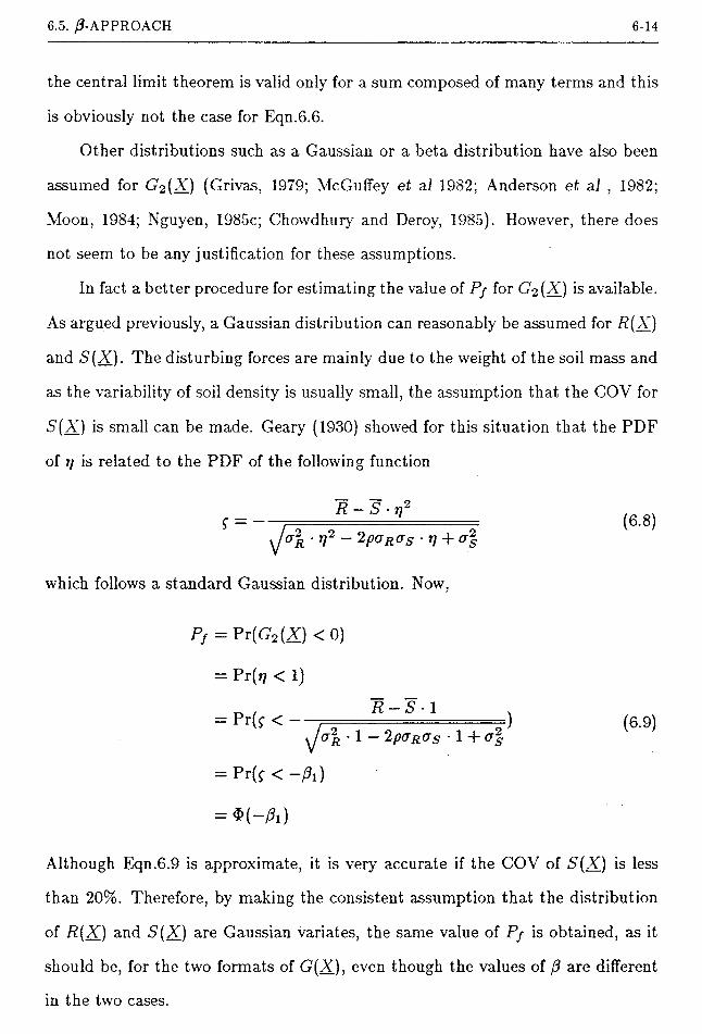
6.5. ^-APPROACH 6-14
the central limit theorem is valid only for a sum composed of many terms and this
is obviously not the case for Eqn.6.6.
Other distributions such as a Gaussian or a beta distribution have also been
assumed for Go(20 (Grivas, 1979; McGuffey et al 1982; Anderson et al , 1982;
Moon, 1984; Nguyen, 1985c; Chowdhury and Deroy, 1985). However, there does
not seem to be any justification for these assumptions.
In fact a better procedure for estimating the value of Pj for Go (20 is available.
As argued previously, a Gaussian distribution can reasonably be assumed for R(X)
and 5(X). The disturbing forces are mainly due to the weight of the soil mass and
as the variability of soil density is usually small, the assumption that the GOV for
5(X) is small can be made. Geary (1930) showed for this situation that the PDF
of ?i is related to the PDF of the following function
___________R - 5 • r;2_______
• r - 2^(75 • t] + o%
which follows a standard Gaussian distribution. Now,
(6.8)
Pf = ?r(G2(X)<0)
= Pt(j] < 1)
= Prk <R-S ■ 1
• 1 - Spends • 1 +<?s
= Pr(f <-A)
= *(-A)
(6.9)
Although Eqn.6.9 is approximate, it is very accurate if the COV of 5(20 ^ess than 20%. Therefore, by making the consistent assumption that the distribution
of R(X_) and 5(20 are Gaussian variates, the same value of Pj is obtained, as it
should be, for the two formats of G(20, even though the values of (5 are different
in the two cases.
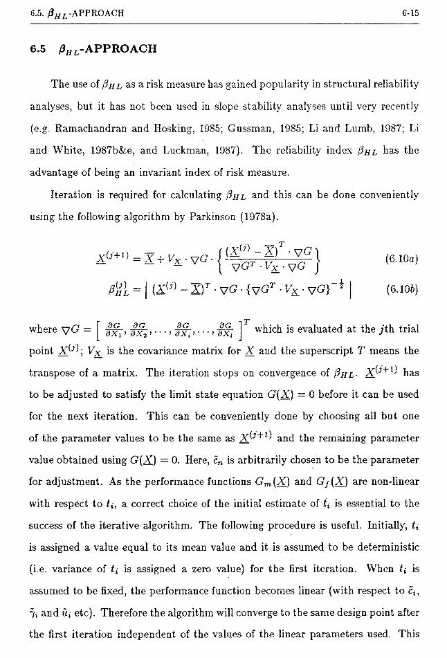
6.5. f3HL-APPROACH 6-15
6.5 /^-APPROACH
The use of Pul as a risk measure has gained popularity in structural reliability
analyses, but it has not been used in slope stability analyses until very recently
(e.g. Ramachandran and Hosking, 1985; Gussman, 1985; Li and Lumb, 1987; Li
and White, 1987b&e, and Luckman, 1987). The reliability index Pul has the
advantage of being an invariant index of risk measure.
Iteration is required for calculating Pul and this can be done conveniently
using the following algorithm by Parkinson (1978a).
X0 + 1) = X+ Vx ■ vG- (Xlj) - X)T ■ yG )VGT ■ ■ VG J
(X0) - X)T • vG' • {vGT ■ Vx • vG'} *
(6.10a)
(6.106)
where yG = which is evaluated at the jth trialax! ’ ax2 ’ • • • ’ ax, > • • • > axt point X^i V\ is the covariance matrix for X and the superscript T means the
transpose of a matrix. The iteration stops on convergence of Pul• + has
to be adjusted to satisfy the limit state equation GfA) = 0 before it can be used
for the next iteration. This can be conveniently done by choosing all but one
of the parameter values to be the same as X_G + l) and the remaining parameter
value obtained using G(X) — 0- Here, cn is arbitrarily chosen to be the parameter
for adjustment. As the performance functions G^fX) and G/(X) are non-linear
with respect to tt, a correct choice of the initial estimate of tt is essential to the
success of the iterative algorithm. The following procedure is useful. Initially, t{
is assigned a value equal to its mean value and it is assumed to be deterministic
(i.e. variance of t{ is assigned a zero value) for the first iteration. When tt is
assumed to be fixed, the performance function becomes linear (with respect to ct,
7i and ul etc). Therefore the algorithm will converge to the same design point after
the first iteration independent of the values of the linear parameters used. This

6.6. METHOD OF PDF FITTING 6-16
‘conditioned’ design point forms a robust starting point for the general iteration.
For a linear performance function with jointly Gaussian random variables,
the reliability index Phl is related to the failure probability via Eqn.2.22. The
equation is often used for other cases of non-linear performance functions and/or
non-Gaussian variables to give a rough estimate of the likely magnitude of the
failure probability.
If the performance function is linear, it can be proved that p and Phl are
equal. The proof is outlined in Appendix B.
6.6 METHOD OF PDF FITTING
In the above two approaches, only the information on the first two statistical
moments of the input parameters are utilized in the analysis. Very often, soil
engineers would have some knowledge on the bounds of the soil properties, either
through subjective judgement or inferred from available soil data. This additional
information cannot be incorporated into the analysis using the above two methods.
In this section, a new approach based on the method of PDF fitting is introduced
whereby the knowledge on the bounds of the soil properties can be utilized to
produce a sharper estimate of failure probability. The method of PDF fitting has
already be outlined in Chapter 2.
To implement the method, the mean value, variance, lower and upper bounds
of the performance function are required. The first two quantities can be obtained
using Equations 6.3 and 6.4. The following discussion addresses the general solu
tion procedure for estimating the bounds of G(X), followed by the presentation of
a simplified solution procedure. A special case of Morgenstern and Price’s method
for which the bounds of G(X) can be calculated analytically will also be discussed.
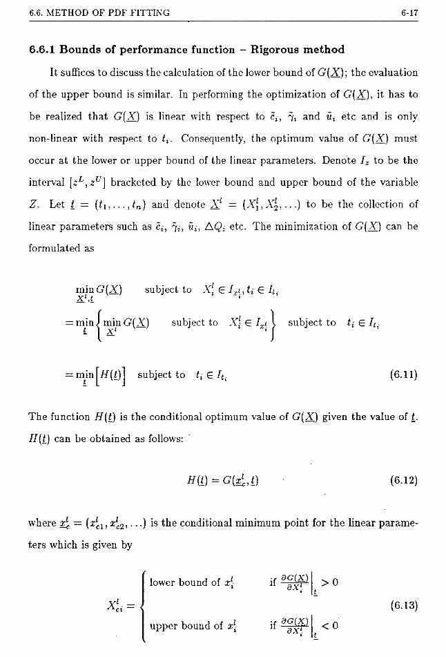
6.6. METHOD OF PDF FITTING 6-17
6.6.1 Bounds of performance function - Rigorous method
It suffices to discuss the calculation of the lower bound of G'(X); the evaluation
of the upper bound is similar. In performing the optimization of G'(X), it has to
be realized that G(X) is linear with respect to ct, 7* and ul etc and is only
non-linear with respect to tt. Consequently, the optimum value of G(X) must
occur at the lower or upper bound of the linear parameters. Denote Iz to be the
interval [zL, zl ] bracketed by the lower bound and upper bound of the variable
Z. Let i — (G,...,fn) and denote X! = (X[, X2, ■ ■ ■) to be the collection of
linear parameters such as ct, 7f/t, AQt etc. The minimization of G'(X) can be
formulated as
The function H(t) is the conditional optimum value of G(X) given the value of f
H(t) can be obtained as follows:
where = (xlci, xlc2, • • •) is the conditional minimum point for the linear parame
ters which is given by
subject to t{ G It,
= min H(t) subject to tx G It (6.11)
H(l) = G(x‘cJ_) (6.12)
/
lower bound of x[ if 77' ^ 0
(6.13)
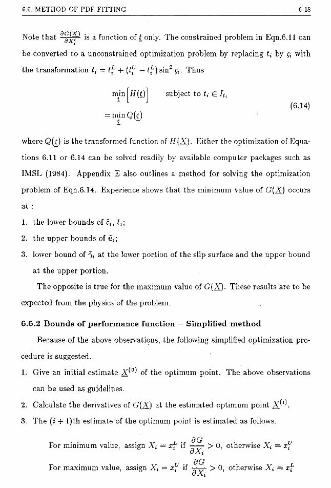
6.6. METHOD OF PDF FITTING 6-18
Note that --^7- is a function of £ only. The constrained problem in Eqn.6.11 can *
be converted to a unconstrained optimization problem by replacing tt by <7 with
the transformation £t = tf + (£[' — tf) sin2 Thus
nnnt H(t)
= min Q(^) f
subject to tt E hx(6.14)
where <3(<r) is the transformed function of II(X_). Either the optimization of Equa
tions 6.11 or 6.14 can be solved readily by available computer packages such as
IMSL (1984). Appendix E also outlines a method for solving the optimization
problem of Eqn.6.14. Experience shows that the minimum value of <S'(AT) occurs
at :
1. the lower bounds of ct, £t;
2. the upper bounds of
3. lower bound of 7; at the lower portion of the slip surface and the upper bound
at the upper portion.
The opposite is true for the maximum value of G'(X). These results are to be
expected from the physics of the problem.
6.6.2 Bounds of performance function — Simplified method
Because of the above observations, the following simplified optimization pro
cedure is suggested.
1. Give an initial estimate of the optimum point. The above observations
can be used as guidelines.
2. Calculate the derivatives of G'(X) at the estimated optimum point
3. The (* + 1)th estimate of the optimum point is estimated as follows.
For minimum value, assign Xt = xf if
For maximum value, assign Xt — if
dGdXtdGJx,
>0,
>0,
otherwise = xf
otherwise Xt = x[
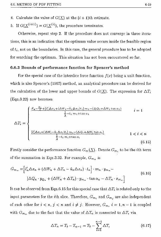
6.6. METHOD OF PDF FITTING 6-19
4. Calculate the value of G(X) at the (« + 1)th estimate.
5. If G(A^! + 1)) = G(X^), the procedure terminates.
Otherwise, repeat step 2. If the procedure does not converge in three itera
tions, this is an indication that the optimum value occurs inside the feasible region
of C, not on the boundaries. In this case, the general procedure has to be adopted
for searching the optimum. This situation has not been encountered so far.
6.6.3 Bounds of performance function for Spencer’s method
For the special case of the interslice force function f(x) being a unit function,
which is also Spencer’s (1967) method, an analytical procedure can be derived for
the calculation of the lower and upper bounds of G(X)- The expression for ATt
(Eqn.3.22) now becomes
Eg —-f [cj Aii + ( AU i —U] Axi)fi|-7»i — (AQi -f AH i tan ct\)
-F — 11 ni] + tan a ii = 1
A Tt =
[c( Ax,- 4- (AIV, — u, Ax,-) t, ] m,—(AQ. + AIV, tan o,)
4—t, m,-f tan a,>, A1 < i < n
(6.15)
Firstly consider the performance function G'm(A). Denote Gm, to be the ith term
of the summation in Eqn.3.32. For example, Gmn is
G, Axn + (AlFn + ATn - unAxn) ■ tn • mn Vm n
[^Qn ■ UQn + (All n + A Tn) • ymn ' tan ctn A Tn • xmn(6.16)
It can be observed from Eqn.6.15 for this special case that ATt is related only to the
input parameters for the ith slice. Therefore, Gmi and Gmj are also independent
of each other for i < n, j < n and i ^ j. However, Gmi i — 1, n — 1 is coupled
with Gmn due to the fact that the value of ATn is connected to ATt via
ATn =Tb- rn_jn — 1
Tb-J2 AT,1=1
(6.17)
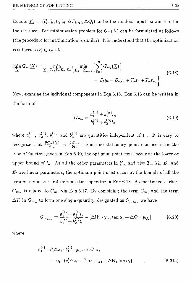
6.6. METHOD OF PDF FITTING 6-20
Denote Y_t = (c', 7t, t{, ul, APt, qu AQt) to be the random input parameters for
the fth slice. The minimization problem for G^fX) can be formulated as follows
(the procedure for maximization is similar). It is understood that the optimization
is subject to c[ £ Ic> etc.1 x
min Gm(X) = x mm mm 777,-Vln.! I
[-^62/6 Eaya -T T Ta.ra]
(6.18)
Now, examine the individual components in Eqn.6.18. Eqn.6.16 can be written in
the form of
(n) (n),fll T d‘2 tn
Gm. =b[n) + b{"}tn
(6.19)
where a\”'\ aX\ 6, and bin' are quantities independent of tn. It is easy to
recognize that . Since no stationary point can occur for the
type of function given in Eqn.6.19, the optimum point must occur at the lower or
upper bound of tn. As all the other parameters in En and also Ta, 1\, Ea and
Eb are linear parameters, the optimum point must occur at the bounds of all the
parameters in the first minimization operator in Eqn.6.18. As mentioned earlier,
GJrin is related to Gm. via Eqn.6.17. By combining the term Gmi and the term
ATt in Gmn to form one single quantity, designated as Gmi+n we have
Ga(*) +
mt+n = -------(Tj-2 - [Aiy* • ymi tana; + AQt ■ yQx\T t>2 11
(6.20)
where
a['} =c[Axt ■ b[:) ■ ym. ■ sec2 at
— oj1 ■ (c[Axl sec2 at + \i ~ A\\\ tan (6.21a)

6.6. METHOD OF PDF FITTING 6-21
(i) _/ &Wia'2 (a
— ulAxl • 6 (0 + ‘ 2/m, sec2 a.
— ojt • (AH^ + \i tan at — iilAxt sec2 a;) (6.216)
i (0 1b\ =— + tan otiA
b <•> -1A
(6.21c)
(6.21c/)
and
^t —2/m, tan xmi + (tn • Tnn tan c*n) • ymn “I- %mn
Ea — ^ — AQi i — 1
-AQi 1 < i < ii
It can also be recognized that dG^E) _ G^»+n . Again, no stationary point
for tt can exist for the function Gm.+n given in Eqn.6.20. Since all the other
parameters in Tt are linear, the optimum point must occurs at the bounds of
all the parameters in Y_l. Consequently, the minimization problem in Eqn.6.18
becomes
Cn — 1 -min Gm(AQ = min J min Gm (X)
X Yn,Ta,Tb,Eb,Ea ^ [ Y.,
-f- Axn T (AH n -F If) nn Axn)bi Vm n ’ Wln
AQnVq„ (AHn 1 b) Vmn tan ctn -F 1 b • xmn
+ {TbXb + Taxa) -F [Lb yb — Eaya) 1 (6.22)
An algorithm for solving Eqn.6.22 is outlined in Fig.6.2. The procedure for
finding the lower and upper bounds of G/(A) is similar. The minimization for

6.6. METHOD OF PDF FITTING 6-22
Given kt = dimension of Y_t gmin=LARGE gmax=SMALL do in = 1,2hn +4
set Y_n, Ta, Tb, Ea, Eb bounds combination tempmin = tempmax = last 3 lines of Eqn.6.22 do i = 1, n — 1
termmin = LARGE termmax = SMALL do it = l,2k>
set Et bounds combination term = Gmi+ntermmin = min(termmin,term) termmax = max(termmax,term)
enddotempmin = tempmin+termmin tempmax = tempmax+termmax
enddogmin = min(gmin,tempmin) gmax = maxfgmax, tempmax)
enddo
Figure 6.2Algorithm for Solving Eqn.6.22. (after Li and White, 1987b)
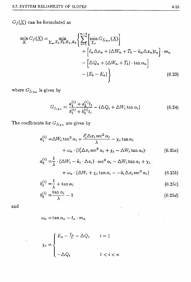
6.7. SYSTEM RELIABILITY OF SLOPES 6-23
Gj(X) can be formulated as
n —1minG/(X)= min J * ~ Yn,Ta,Tb,Ea,Eb \
minG/i+n(X)
+ \c„ Ai„ + (AWn + Tb-
AQn + (AWn + Tb) • tan c*n
-(Eb-Ea)
where Gfi+n is given by
a*'1 + ai'kj
/,+n 6<*> + 6<*)<,- (A(Jt + AW{ tan or,-)
The coefficients for Gfi+n are given by
and
=AW, tan2 a, + :i-s—tt* - x, tana,a
+ cjn • (clAxl sec2 ctl -f Xi ~ AWt tan a,-)-
a^ =— • (AW{ — iii • Axt) • sec2 at — AWt tan a; -f \iA
+ cjn • (AWi + Xi tan at-----ut Axt sec2 at)
b[l) =- + tan atA
^(t) _tan cxt 1——-1
cdn — tan cxn tn • Tnn
Ea-^f- AQ, 1 = 1
Xi = <
• mn
(6.23)
(6.24)
(6.25a)
(6.256)
(6.25c)
(6.25rf)
l-A Qt 1 < i < n

6.7. SYSTEM RELIABILITY OF SLOPES 6-24
6.7 SYSTEM RELIABILITY OF SLOPES
So far discussion has concerned the failure probability for a particular slip
surface. In fact, there are infinitely many admissible slip surfaces although the
failure probability of each of them may differ. The slope should be considered
as a system in series. Each component represents a feasible slip surface. Failure
of any slip surface (component) will imply the failure of the slope (the system).
The system failure probability of the slope should be evaluated using the system
reliability theory, although it is not an easy task and no suitable procedure is yet
available for its calculation.
The system failure probability Pfs of slopes is bounded by (Cornell, 1967)
(Pf) max < ^/s < 1 (6.26)
where (P/)mdLX is the failure probability for the most critical slip surface. If high
correlation exists between different slip surfaces, the system failure probability
will be close to the lower bound. A study by Morla Catalan (1974) on cohesive
slopes indicated that the system failure probability wa5 significantly higher than
(f/)max for the normal range of correlation existing for real slopes. However, the
sampling uncertainty (which is perfectly correlated) had not been considered in the
analysis and hence the correlation between slip surfaces would be underestimated.
Therefore, the conclusion may not be true in general. More research needs to be
done before any definite conclusions can be drawn.
Although a complete analysis of system failure probability is not available,
the value of (P/)max can serve as a convenient and valuable index in assisting the
engineer to exercise judgement in the design of slopes. The procedure for locating
the critical slip surface is discussed in Chapter 7.
It must be pointed out that some misconceptions concerning this system reli-
ablity of slopes exist in the literature. Grivas et a/ (1979) and McPhail and Fourie

6.8. PROBABILISTIC MODELLING OF PORE-WATER PRESSURE 6-25
(1985) treated the location of the slip surface as another random variable in the an
alysis and assigned a certain probability distribution for it. Grivas et al (1979) also
evaluated the ‘mean’ location of the slip surface. This is a misconception because
although the position of the slip surface is an important factor to be considered
in the analysis, it is by no means a random variable. To explain this, consider a
simple analogy of a portal frame having two plastic collapse mechanisms, Al and
A2. Each failure mechanism can be likened as the failure of a slip surface in a
slope. As the system is in series, the system failure probability of the portal frame
can be calculated as
Pfs = PrfAj U An) = Pr(Al) + Pr(A2) - Pr(Al D A2) (6.27)
As individual slip surfaces are treated as failure events in the analysis, the mean
location of the slip surface, which can be likened as the mean collapse mode of a
portal frame, bears no meaning in system reliability theory.
6.8 PROBABILISTIC MODELLING OF PORE-WATER PRESSURE
Pore-water pressure fluctuation within a slope is always difficult to predict.
It is influenced among other things by the spatial variability of hydrological prop
erties of soil, location and undulation of bed rock stratum, local distribution of
rainfall, variation of vegetation cover and presence of joints in the soil profile*.
The situation is aggravated by the fact that the variability of hydrological prop
erties of soil is often large. A commonplace COV of permeability of soils is larger
* The presence of joints will greatly affect the local variation of water flow. It
may also give rise to the formation of a soil pipe (Pierson, 1983). Some of the
slope failures in Hong Kong can be attributed to local built-up of water pressure
in the soil pipes (Brand et a1 , 1986).

6.8. PROBABILISTIC MODELLING OF PORE-WATER PRESSURE 6-26
than lOO^c. The sampling uncertainty is therefore high.
Although the importance of pore-water pressure has long been recognized in
slope stability designs, theoretical studies on stochastic modelling of water pres
sure fluctuation started only within the last decade or so (e.g. Smith and Freeze,
1979aAb; Chirlin and Dagan, 1980; Andersson and Shapiro, 1983; Kitanidis and
Vomvoris, 1983; Bergado and Anderson, 1985; Anderson and Howes, 1985; Lee
and W u. 1987). In these analyses, the hydrological properties of soils are modelled
as random fields and the response (which may be the rise of water level or others)
is predicted using the relevant differential equation governing the flow of water.
The mean value and variance of the predicted response are calculated using, typ
ically, a stochastic finite element method or simulation. At present, literature on
statistical analysis of measured water pressure fluctuation is extremely scarce. The
validity of the above theoretical models has yet to be verified.
A detailed study of pore-water pressure fluctuation is beyond the scope of the
present study. In this section, two simple models are proposed for characterizing
the uncertainty of pore-water pressure. In the first model, the pore-water pressure
is described by means of the pore-water pressure ratio rx which is defined as
= rx ■ ArnAij
(6.28)
where Ar,, Ax and r)l are respectively the width, the area and average soil density
for slice i. rt is treated as a random variable in the analysis.
In the second model, the variation of pore-water pressure is characterized by
three phreatic surfaces as shown in Fig.6.3. yu(x) represents the upper bound of
the water level, yP(x) the most probable location and yi(x) the lower bound. The
average water pressure ut acting on the slice base can be approximated by

6.8. PROBABILISTIC MODELLING OF PORE-WATER PRESSURE 6-27
Figure 6.3 Modelling of Pore-water Pressure
lw(wi ~ Vi) = lw ’ hi h> 0
0 h< 0
= lw ■ {Wi - Vi) • H(v)i - Vi)
— lw ' hi ' H
(6.29)
where iw is the unit weight of water and H( ) is the unit step function. The
location n\ of the phreatic surface becomes a random variable.
To evaluate the mean and variance of wt, it is required to know the PDF of
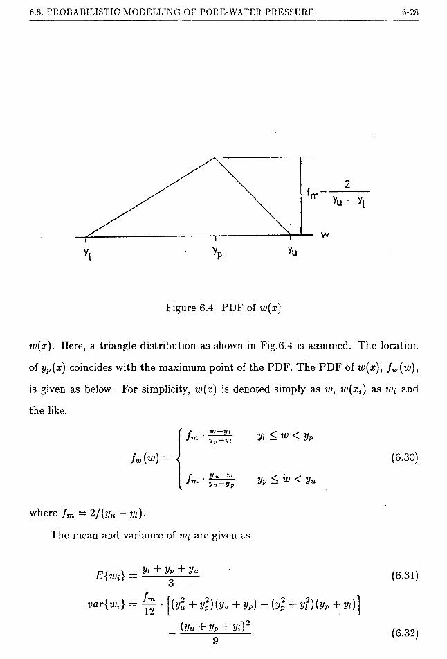
6.8. PROBABILISTIC MODELLING OF PORE-WATER PRESSURE 6-28
2
Vu ~ yl
Figure 6.4 PDF of w(x)
w(x). Here, a triangle distribution as shown in Fig.6.4 is assumed. The location
of yp(x) coincides with the maximum point of the PDF. The PDF of w(x), fw(w),
is given as below. For simplicity, w(:r) is denoted simply as w, w(xt) as wt and
the like.
fw (u>) =
fr
fr
w—yiyp-yi
Vu—rjuy«-yP
yi <w < yp
yP < w < yu
(6.30)
where fm = 2/(yu - yi).
The mean and variance of wt are given as
E{wt)
var{w{}
yi + yP + Vu3
fm~12 (yl + Vp)(yu + yP) - (yl + y?){yP + yi)
(yu + yP + yi)2
(6.31)
9(6.32)

6.9. ILLUSTRATIVE EXAMPLES 6-29
In theory, the variation of water pressure can be modelled as a random field as is
done in Luckman (1987). At present, little is known about the correlation struc
ture of water pressure. It is speculated that it may consists of two components,
one governed by the changes in regional water system with a scale of fluctuation
perhaps comparable to the scale of the slope and the other governed by location
variation of soil properties having a scale of fluctuation comparable to that of soil
properties. Pending more information on water pressure fluctuation, it is assumed
tentatively herein that the water pressure is perfectly correlated across the slope.
This would imply that the entries of the autocorrelation matrix for rt or wt are
all equal to 1.
6.9 ILLUSTRATIVE EXAMPLES
In this section, the implementation of the probabilistic approach will be de
picted by means of illustrative examples. The assumptions used in the following
discussion are discussed first.
1. In the analysis, only c[, tt and ul are taken as random variables. Other
loads (Ea, qx, APt, AQt) are taken as zero. The effect of a tension crack is also
neglected.
2. Little has been published in current literature on the joint PDF of soil prop
erties. Under controlled conditions such as constant soil density and moisture
content, Matsuo and Kuroda (1974) observed a strong negative correlation
between the strength components c and t. However, for natural soils, evi
dence (Lumb, 1970; Schultze, 1975) shows almost zero correlation between the
strength parameters while significant negative correlation has been reported by
Forster and Weber (1981) and Grivas (1981). However, the strength compo
nents c' and t are treated herein as independent for simplicity. The assumption
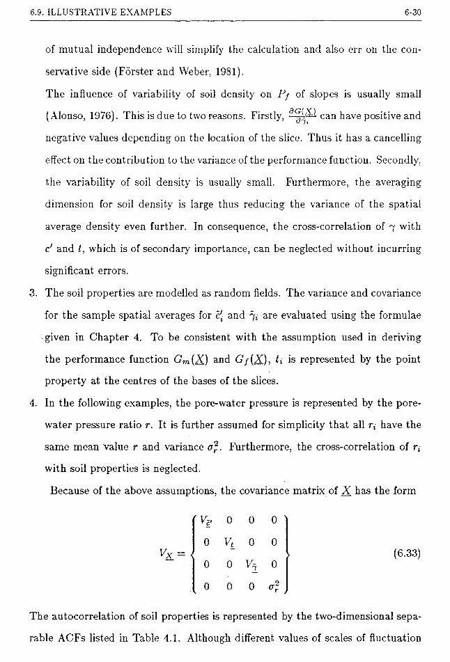
6.9. ILLUSTRATIVE EXAMPLES 6-30
of mutual independence will simplify the calculation and also err on the con
servative side (Forster and Weber, 1981).
The influence of variability of soil density on Pj of slopes is usually small
(Alonso, 1976). This is due to two reasons. Firstly, can have positive and
negative values depending on the location of the slice. Thus it has a cancelling
effect on the contribution to the variance of the performance function. Secondly,
the variability of soil density is usually small. Furthermore, the averaging
dimension for soil density is large thus reducing the variance of the spatial
average density even further. In consequence, the cross-correlation of 7 with
c' and t, which is of secondary importance, can be neglected without incurring
significant errors.
3. The soil properties are modelled as random fields. The variance and covariance
for the sample spatial averages for c[ and 7i are evaluated using the formulae
given in Chapter 4. To be consistent with the assumption used in deriving
the performance function Gm(T) and G/(X), tt is represented by the point
property at the centres of the bases of the slices.
4. In the following examples, the pore-water pressure is represented by the pore-
water pressure ratio r. It is further assumed for simplicity that all rt have the
same mean value r and variance Furthermore, the cross-correlation of rl
with soil properties is neglected.
Because of the above assumptions, the covariance matrix of X has the form
(V?
Vx =
0 1
0 Vt 0 0
0(6.33)
The autocorrelation of soil properties is represented by the two-dimensional sepa
rable ACFs listed in Table 4.1. Although different values of scales of fluctuation

6.0. ILLUSTRATIVE EXAMPLES 6-31
can be used for different soil properties, they are assumed to be equal.
T = /v f (x) * E
f(x)r constant
f(x) = half - sine
Figure 6.5 Types of Interslice Force Function
Two interslice force functions as shown in Fig.6.5 are used. Unless stated
otherwise, results presented below are based on the simple exponential ACF (Type
I), equal values of 8X and <5y, i.e. 8X = 8y = 6 and the constant interslice function.
The reliability index P and Phl are related to the failure probability using Pj —
$(—/?) and Pj — <&(—(3hl) respectively. Fig.6.6 shows the variation of Pj with
the reliability index (3 or Phl-

failu
re
prob
abili
ty
6.9. ILLUSTRATIVE EXAMPLES 6-32
reliability index
Figure 6.6 Variation of Pj with Reliability Index

6.9. ILLUSTRATIVE EXAMPLES 6-33
6.9.1 Example 6.1
centre of momentc
Figure 6.7 Geometry of Slope for Example 6.1
The geometry of the slope is shown in Fig.6.7. 10 slices are used through
out and the sample size Ar is taken arbitrarily to be 8. The following are input
parameters of the soil.
mean cov 1. bounds u. bounds
c' 18 kN/m2 20% 3.6 kN/m2 34.2 kN/m2
18 kN/m3 5% 15.3 kN/m3 20.7 kN/m3
t tan 30° 10% tan 25° tan 35°
r 0.2 10% 0.15 0.25
6.9.1.1 Adjustment of X
Fig.6.8 shows the typical variation of /?, (3hl and Pjj with A. The intersection
point of the curves gives the so-called ‘rigorous’ solution and the corresponding
value of A is denoted as Amf- At this point, the probability predicted from the
performance functions Gm(X) and G/(X) are equal. It can be observed that the

6.9. ILLUSTRATIVE EXAMPLES 6-34
P
Phl
pff
Figure 6.8 Variation of (a) f3 (b) (3hl and (c) Pff with A
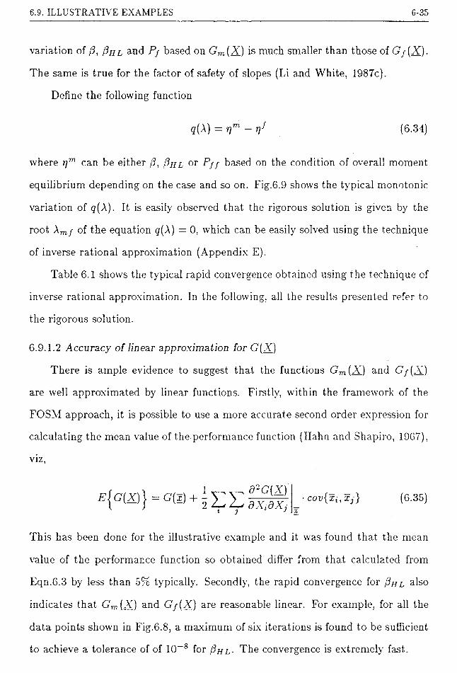
6.9. ILLUSTRATIVE EXAMPLES 6-35
variation of j3, Phl and Pj based on Gm(X_) is much smaller than those of G f(X).
The same is true for the factor of safety of slopes (Li and White, 1987c).
Define the following function
9(A) = r,m - ,/ (6.34)
where r]m can be either p, 3hl or Pff based on the condition of overall moment
equilibrium depending on the case and so on. Fig.6.9 show's the typical monotonic
variation of (7(A), It is easily observed that the rigorous solution is given by the
root Amf of the equation g(A) = 0, which can be easily solved using the technique
of inverse rational approximation (Appendix E).
Table 6.1 shows the typical rapid convergence obtained using the technique of
inverse rational approximation. In the following, all the results presented refer to
the rigorous solution.
6.9.1.2 Accuracy of linear approximation for G(X)
There is ample evidence to suggest that the functions Gm(X) and Gf(X_)
are w'ell approximated by linear functions. Firstly, within the framework of the
FOSM approach, it is possible to use a more accurate second order expression for
calculating the mean value of the performance function (Hahn and Shapiro, 1967).
viz,
E r,,_, d-G{X)(£) + 2 E E dX.d.X, cov{xt, ary} (6.35)
This has been done for the illustrative example and it was found that the mean
value of the performance function so obtained differ from that calculated from
Eqn.6.3 by less than typically. Secondly, the rapid convergence for (3hl also
indicates that Gni(Ay) and G/(X) are reasonable linear. For example, for all the
data points shown in Fig.6.8, a maximum of six iterations is found to be sufficient
to achieve a tolerance of of 10~s for Phl- The convergence is extremely fast.

6.9. ILLUSTRATIVE EXAMPLES 6-36
fW
Leqend
° f(x)= constant
a f(x) = half - sin e
simplified Bishop's method
6 = 10 m
simplified Jan bus method
-0.2 -
-0.4 -
-0.6 -
Figure 6.9 Variation of q(A)
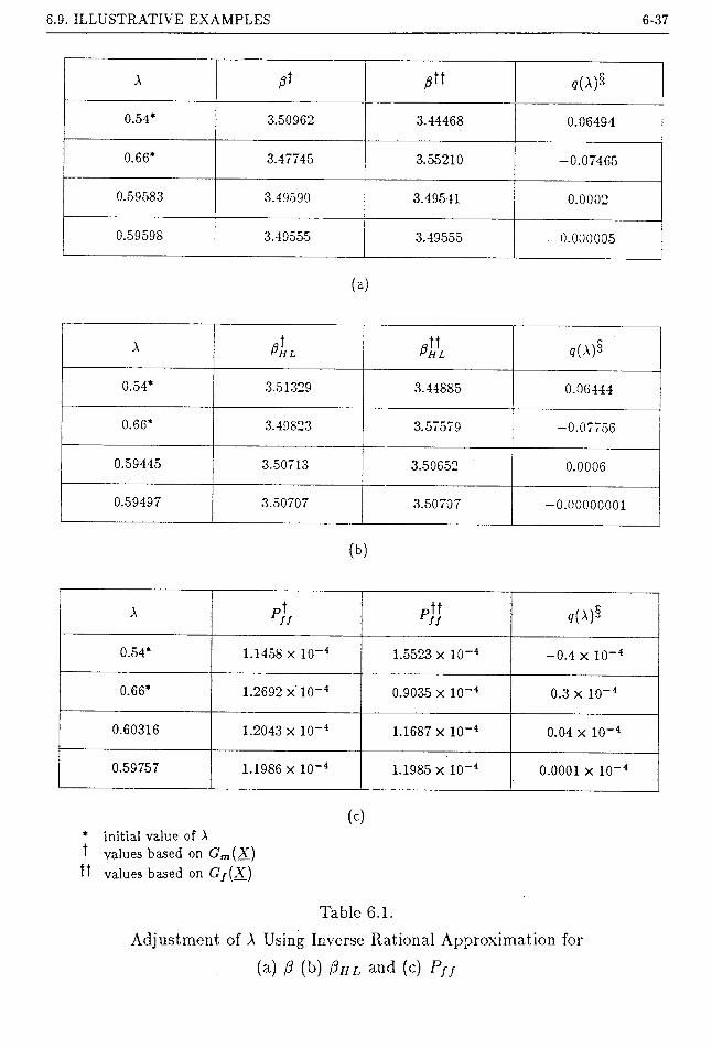
6.9. ILLUSTRATIVE EXAMPLES 6-37
A ,(A)§
0.54* 3.50962 3.44468 0.06494
0.66* 3.47745 3.55210 -0.07465
0.59583 3.49590 3.49541 0.0002
0.59598 3.49555 3.49555 0.000005
A 4 j. *ttPhl ,(A)§
0.54* 3.51329 3.44885 0.06444
0.66* 3.49823 3.57579 -0.07756
0.59445 3.50713 3,50652 0.0006
0.59497 3.50707 3.50707 -0.00000001
(b)
A ptrJI
pttrff «(A)S
0.54* 1.1458 x 10-4 1.5523 x 10"4 -0.4 x 10“4
0.66* 1.2692 x 10-4 0.9035 x 10~4 0.3 x 10~4
0.60316 1.2043 x 10"4 1.1687 x 10"4 0.04 x 10~4
0.59757 1.1986 x 10~4 1.1985 x 10~4 0.0001 x 10“4
(c)
* initial value of Avalues based on Gm(X_)
tt values based on Gj[X_)
Table 6.1.Adjustment of A Using Inverse Rational Approximation for
(a) (3 (b) (3hl and (c) Pff

6.9. ILLUSTRATIVE EXAMPLES 6-38
Pf <Phl>
5= 1 m
8=8 = 88= 5m
8=10m
Figure 6.10 Failure Probability Plot inferred from (3 and Phl
6.9. ILLUSTRATIVE EXAMPLES 6-39
As mentioned earlier, the values of p and Phl are equal if the performance
function is linear. Fig.6.10 shows the failure probability plot inferred from for [3
and Phl- The close agreement between the two values provides the third evidence
that a linear approximation is very accurate for Gm(X) and G/(X). As the values
of Pf inferred from (3 and Phl are similar, only results for Phl will be presented
below.
6.9.1.3 Comparison of different approaches
As mentioned earlier, values of Pj inferred from p and Phl are essentially
the same. This can be attributed to the minimal non-linearity of the performance
function formulated in terms of the safety margin. A larger difference between p
and Phl has been reported by Luckman (1987) for a slope in Hong Kong. This
may be due to their use of Go(X) (see Section 6.4) for the formulation of the
performance function giving rise to a higher degree of non-linearity and hence a
larger error in the calculation of mean and variance of the performance function
which is then reflected in the larger difference in two reliability indices.
Fig.6.11 shows the probability plot of the failure probabilities inferred from
Phl and the method of PDF fitting. It can be seen that the value of Pjf is
smaller than the values inferred from Phl (and also p). This is to be expected as
the approaches using p and Phl assume a unbounded tail for the distribution of
G(X)• In consequence, the probability inferred from a PDF with infinite tail will
be greater than that from a cut-off tail. At high probability level, the difference in
values is small. However at lower probability level, the values of Pf inferred from
P and Phl are conservative.
6.9.1.4 Influence of interslice force function on Pj
Fig.6.12 shows a comparison of Phl obtained for two different interslice force
functions. Although the constant and half-sine interslice force functions are vastly
different, the values of Phl are almost identical. Similar results are also obtained

6.9. ILLUSTRATIVE EXAMPLES 6-40
Pf (PhiJ
o Type IType IIType IIIType IV
6 = 1 m
8 = 5m
8= 1 0m
Pff
Figure 6.11 Failure Probability Plot inferred from /3hl and Pff

6.9. ILLUSTRATIVE EXAMPLES 6-41
Phl
A C FType IType IIType III
• Type IVu) 4.0 -
35 -
6 =10 m
f(x)= constant
Figure 6.12Comparison of Phl for Different Interslice Force Functions
for P and Pjf indicating that the failure probability of slopes is not sensitive to
the interslice function provided of course it is not very unreasonable.
6.9.1.5 Influence of the form of ACF on Pj
In probabilistic design of slopes, the order of magnitude of Pj is of more con
cern than its absolute value. It can be concluded from Figures 6.10, 6.11 and 6.12
along with other studies by the Author that the value of Pj is not very sensitive
to the type of the ACF used. All the four types of ACF used in this work give val-

6.9. ILLUSTRATIVE EXAMPLES 6-12
ues of Pf with the same order of magnitude. The scale of fluctuation has already
captured the essential correlation structure of soil properties. A similar conclusion
has also been drawn by Luckman (1987). This 1ms significant practical implica
tions as the exact form of ACF is difficult to estimate in practice without a large
number of samples. Because of the simplicity of Type I ACF, it is recommended
for general use.
6.9.1.6 Influence of scale of fluctuation
Fig.6.13 shows the variation of Pf inferred respectively from 3hl and PDF
fitting with the scale of fluctuation. A Type I ACF (simple exponential) was
used in the calculation. It can be seen that Pj is very sensitive to the value of
<5, although it does not depend significantly on the function form of the ACF as
mentioned earlier. Therefore, more attention must be paid to the estimation of
this important parameter in soil investigation. Fig.6.13 reinforces the discussion
in Section 6.3, that ignoring the variance reduction due to spatial averaging results
in an astonishingly large value of Pf.
6.9.1.7 Location of Critical Slip Surface
Circular slip surfaces are considered first. Table 6.2 summarizes the positions
of the critical slip circles for different cases (<5 =5m). The locations of the critical
slip circle with minimum /?, (3hl and maximum Pjj are different, but they are
close to the critical slip circle with minimum factor of safety which is centred at
(-1,14).
Fig.6.14 compares the positions of critical non-circular slip surface with the
critical slip circles with minimum factor of safety or reliability index (3. It can be
seen that these surfaces are very close to each other. As the evaluation of failure
probability or reliability index requires more effort than the factor of safety, it is
preferable to search for the critical slip surface with the minimum factor of safety

6.9. ILLUSTRATIVE EXAMPLES 6-43
Pf ( Phl>
20 m
20 m
Figure 6.13Variation of Pj inferred from (a) (b) Pjf
With Scale of Fluctuation
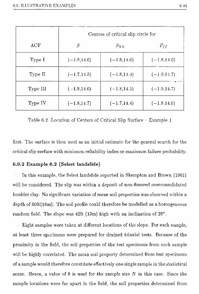
6.9. ILLUSTRATIVE EXAMPLES 6-44
Centres of critical slip circle for
ACF P Phl Pff
Type I (-1.8.14.6) (-1.8,14.6) (-1.8,14.6)
Type II (-1.7,14.3) (-1.8,14.4) (-1.9,14.7)
Type III ( — 1.8,14.6) (—1.8,14.5) (-1.9,14.7)
Type IV (-1.8,14.7) ( — 1.7,14.4) (-1.8.14.6)
Table 6.2 Location of Centers of Critical Slip Surface - Example 1
first. The surface is then used as an initial estimate for the general search for the
critical slip surface with minimum reliability index or maximum failure probability.
6.9.2 Example 6.2 (Selset landslide)
In this example, the Selset landslide reported in Skempton and Brown (1961)
will be considered. The slip was within a deposit of non-fissured overconsolidated
boulder clay. No significant variation of mean soil properties was observed within a
depth of 60ft(18m). The soil profde could therefore be modelled as a homogeneous
random field. The slope was 42ft (13m) high with an inclination of 28°.
Eight samples were taken at different locations of the slope. For each sample,
at least three specimens were prepared for drained triaxial tests. Because of the
proximity in the field, the soil properties of the test specimens from each sample
will be highly correlated. The mean soil property determined from test specimens
of a sample would therefore constitute effectively one single sample in the statistical
sense. Hence, a value of 8 is used for the sample size N in this case. Since the
sample locations were far apart in the field, the soil properties determined from
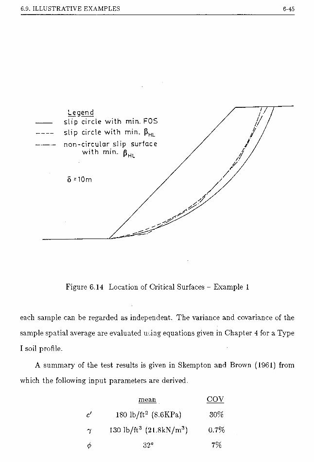
6.9. ILLUSTRATIVE EXAMPLES 6-45
Legendslip circle with min. FOSslip circle with min. |3HL
non-circular si ip surface with min. R̂
H L
5 = 10m
Figure 6.14 Location of Critical Surfaces - Example 1
each sample can be regarded as independent. The variance and covariance of the
sample spatial average are evaluated using equations given in Chapter 4 for a Type
I soil profile.
A summary of the test results is given in Skempton and Brown (1961) from
which the follow ing input parameters are derived.
mean COY
180 lb/ft2 (8.6KPa) 30%
130 lb/ft3 (21.8kN/m3) 0.7%
7%
7
0 32

6.9. ILLUSTRATIVE EXAMPLES 6-46
Using a first order Taylor’s series approximation, the mean value and COV of
t (i.e. tan<^') are given as tan 32° and 9% respectively. A mean value of 0.45 was
suggested by Skempton and Brown (1961) as a suitable value for the pore-water
pressure ratio r of the slope. A judgemental value of 10% is assumed herein for
the COV of r.
no. of samples
6= 5ft
6 = 15ft
Height of slope ,H (ft)
Ll_
Oto
«*—
_ooa
Ljl
Figure 6.15
Variation of Failure Probability With Height
of Slope (Selset Landslide)
Fig.6.15 show's the variation of the failure probability with the height of the
slope. The reliability index Pul is based on Gm(2Q and a value of 0.6 for A. The

6.9. ILLUSTRATIVE EXAMPLES 6-47
results presented in the figure correspond to the minimum value of Phl associated
with the critical slip surface. A toe failure is assumed throughout. It is also
assumed that the mean and variance of r are unaffected by the change in the
height of the slope. Since the scale of fluctuation of the soil properties are not
known, two values of 6 are used - 5ft (1.5m) and 15ft (4.6m). The results are
plotted in solid lines in Fig.6.15. For the actual slope height of 42ft (12.8m), the
failure probability of the slope is high (>50%). This is to be expected as the
failure of the slope had indeed occurred. As the slope height decreases, the factor
of safety increases and the difference in Pj given the two values of 8 becomes more
pronounced.
Assuming that the COY of the soil properties remains unchanged, the slope
was re-analyzed using a value of 30 for the sample size N. Since the sample size
is now larger, the sampling uncertainty is reduced resulting in a smaller value of
Pj. Note that the increase in reliability of the slope due to an increase in sample
size is greater for the case of 8 =5ft (1.5m). In fact, it is generally true that
increasing the sample size for soils with a smaller value of 8 is more effective in
reducing the failure probability than soils with a larger value of 8. It is because
when the scales of fluctuation is large compared with the dimensions of the slope,
the reduction in variance due to spatial averaging would be smaller. The variance
of the sample spatial average would then be dominated by the spatial variability
of the soil properties. An large increase in the sample size N can only reduce the
total variance by a small amount.
In the design of soil slopes, results like Fig.6.15 can be obtained using the prior
knowledge of the soil properties. This kind of information would be very useful
in the design stage for identifying the critical parameters to which more attention
should be paid and for determining a suitable sample size for soil testing.

CHAPTER 7
LOCATION OF CRITICAL SURFACE
7.1 INTRODUCTION
The reliability analysis of the stability of a slope involves two steps; one for
the calculation of the failure probability of a particular slip surface and the other
for locating the most critical slip surface which has the maximum risk. The former
has been discussed in Chapter 6. This chapter addresses the latter topic.
A number of approaches have been developed over the past decade for locating
the critical slip surface with the minimum factor of safety. The following briefly
reviews the existing approaches and the possibility of extending some of these
methods to the searching of critical slip surface in the context of probabilistic
analysis will also be discussed.
Garber (1973) and Baker and Garber (1977a, 1977b& 1978) presented a series
of papers on the application of calculus of variations to locating the critical slip
surface with the minimum factor of safety. In their approach, the functionals,
deduced from the consideration of the overall vertical, horizontal and moment
equilibrium, were minimized analytically with respect to the location y(x) of the
slip surface and the normal stress distribution a{x) along it. The general solution,
even for the simplest case of a homogeneous soil profile, requires the solving of the
Euler’s differential equation in addition to the determination of seven unknown
7-1

7.1. INTRODUCTION 7-2
quantities (Baker and Garber, 1977b). Although the theoretical analysis based on
the calculus of variations gives greater insight to the method of limit equilibrium
in slope stability analysis and gives the smallest possible factor of safety with
no ‘arbitrary’ assumption about the internal force is required as emphasized by
Baker and Garber, it is difficult to use in practice. It is perhaps this that led Baker
(1980) to give up this analytical approach and revert to an approximate numerical
approach based on dynamic programming and the adoption of Spencer's method
of slope analysis.
Castillo and Revilla (1977) and Revilla and Castillo (1977) also presented a
theoretical study based on the calculus of variations. The approach is similar to
that by Baker and Garber except that the functionals to be optimized were now
based on the simplified Janbu method. That is to say, the distribution of normal
stress cr(x) is inferred by the assumption about the interslice forces rather than
obtained by means of calculus of variations.
The calculus-of-variation approach is entirely an deterministic approach. The
use of the method is very limited in the context of probabilistic design. The
difficulty arises from the fact that the functional of the failure probability cannot
be expressed as an explicit function of the location of the slip surface.
A different approach based on the random generation of slip surfaces was
developed by Boutrup and Lovell (1980). A series of admissible slip surfaces
are generated randomly and the critical slip surface with the smallest value of
the factor of safety is selected from those generated surfaces. Theoretically, the
method can also be used to locate the critical slip surface with the maximum
failure probability. However, it has the disadvantage that a lot of effort is wasted
in evaluating the failure probability of the surfaces which are far from the critical
surface and there is always a statistical uncertainty as regards to whether the
critical surface so obtained is the most critical slip surface or not.

7.1. INTRODUCTION 7-3
Baker (1980) defined the slip surface by a number of nodal points joined
together by straight lines and used dynamic programming to determine the most
critical slip surface. However, Baker’s (1980) method has the disadvantage that
it is only applicable to Spencer’s (1967) method as explained in Li and White
(1987a). Furthermore, the return function cannot be formulated in a probabilistic
analysis and hence the dynamic programming approach cannot be used.
Celestino and Duncan (1981), Nguyen (1985b) and Li and White (1987a)
also described the slip surface by means of nodal points and the factor of safety is
treated as a multivariate function defined implicitly with respect to the coordinates
of the nodal points. The critical slip surface associated with the minimum FOS is
then obtained by optimizing the factor-of-safety function with respect to the nodal
coordinates. By defining the reliability-index function or the failure-probability
function in term of the nodal coordinates, the same approach can also be adopted
for locating the critical slip surface with the minimum reliability index or maximum
failure probability. The method is quite general and is valid for any stability
models. Of course, the viability of the method depends largely on the amount
of effort required for the optimization. Celestino and Duncan (1981) and Li and
White (1987a) used the alternating-variable approach in searching for the optimum
while Nguyen (1985b) adopted the simplex approach.
The success of the optimization approach has been demonstrated by Li and
White (1987a) for the calculation of the minimum factor of safety of a slope. How
ever, when applied to the calculation of the reliability index or the failure prob
ability, it has to be remembered that the calculation of these quantities requires
much more computing time than the calculation of the factor of safety. Although
the simple technique of alternating variables is adequate for finding the minimum
factor of safety, a more efficient optimization technique is desirable for locating
the critical surface with the minimum reliability index or maximum probability.

7.2. DEFINITION OF PROBLEM 7-4
In the following, the technique of steepest decent is used for the optimization of
the objective function.
7.2 DEFINITION OF PROBLEM
The problems of locating the most critical position for circular and non-
circular slip surfaces are different. They will be discussed separately in this section.
7.2.1 Non-circular slip surface
The following is a unified treatment of non-circular surfaces. Fig.7.1 shows
the position of a slip surface defined by a series of straight lines. The coordinates
of the 7th nodal point are denoted by (:rt, yt). As the coordinates (x^y,) vary,
they trace out infinitely many slip surfaces which are kinematically admissible.
The nodal points can be divided into two categories:
(i) Unconstrained nodal points (U)
For unconstrained nodal points, the abscissa xt and ordinate yt can vary
independently. Point B and E in Fig.7.1 are examples of unconstrained nodal
points.
(ii) Nodal points on prescribed curve (C)
Very often, the development of a slip surface is influenced by the presence
of a weak soil seam or strong rock layer. As in the case of Fig.7.1, points
C and D should only move in the direction parallel to the weak soil seam.
Other examples of of class C nodal points are points A and F in Fig.7.1. If
xd represents the initial abscissa of point D, the ordinate of the point will be
given by
vd = v(id +$d) (7.1)
where y(-) is the function describing the trajectory' of the nodal point along

7.2. DEFINITION OF PROBLEM 7-5
F
y
Figure 7.1 Definition of Slip Surface by Nodal Points

7.2. DEFINITION OF PROBLEM 7-6
the prescribed curve and sB is the horizontal distance of the point measured
from xB. The variable sB becomes the location parameter of the nodal point.
Define the risk function H(X_) to be either the factor of safety, reliability index
or the failure probability of a slip surface with location parameters X_. Suppose
that there are k class U nodal points and m class C nodal points. Without loss
of generality, the k nodal points of class U are represented as (sq, yt),i — 1, k and
location parameters of the class C points are denoted by Si,i = l,m. The risk
function can therefore be written as a multivariate function as follows;
H(X) = H(xl,x2,--- ,xk;yi,y2,---,yk\si,s2,---,sm)(7.2)
and 2 k + m = n
To locate the most critical slip surface is therefore equivalent to finding the 72-
dimensional minimum point and the minimum value for the function H. Some
constraints exist in an implicit form for the variables of the risk function. It can
be discerned by referring to Fig.7.1. The nodal points of the slip surface must be
in the order A-B-C-D-E-F. Therefore, the abscissa of the nodal points must satisfy
xA < xB < xc
xB <xc < xD (7.3)
xc <xD < xB etc.
Furthermore, the ordinates of the points must lie within the slope. Bell (1969)
also made further restrictions regarding the convexity of the slip surface.
7.2.2 Circular slip surface
The treatment for circular slip surfaces is simpler than for non-circular sur
faces. For circular slip surfaces, there are only three location parameters; namely
the abscissa xQ and the ordinate y0 of the centre of the slip circle as well as the

7.3. SEARCHING PROCEDURE 7-7
radius R of the circle. The risk function can be written as a function of these three
variables.
H(X) = H(x0,y0,R) (7.4)
Optimizing the function H(X_) will give the minimum value of F, the minimum
reliability index or the maximum failure probability depending on the case and
also the centre and radius of the most critical slip circle. Very often, the geology of
the slope dictates the radius of the slip circles. In these cases, the function H[X)
reduces to a function of the coordinates of the centre of the slip circle.
For both circular and non-circular slip surfaces, the minimum point and the
minimum value for the function H(X) can be obtained using the optimization
techniques for a multivariate function. The procedure is described in the following
section.
7.3 SEARCHING PROCEDURE
In an earlier work (Li and White, 1987a), the Author used the alternating-
variable approach for optimizing the factor-of-safety function of a slope. In this
work, the method of steepest descent will also be used. The method is generally
more efficient than the alternating-variable approach especially for non-circular
slip surfaces which have more location parameters than circular slip surfaces. The
alternating-variable technique and the method of steepest descent are well doc
umented in the literature (e.g. Beveridge and Schechter, 1970; Jacoby et a 1 ,
1972). A brief outline of the two methods is given in Appendix E. Here, some
useful procedures which have been incorporated into the computer program will
be discussed.
The derivatives of the risk function required in the implementation of the
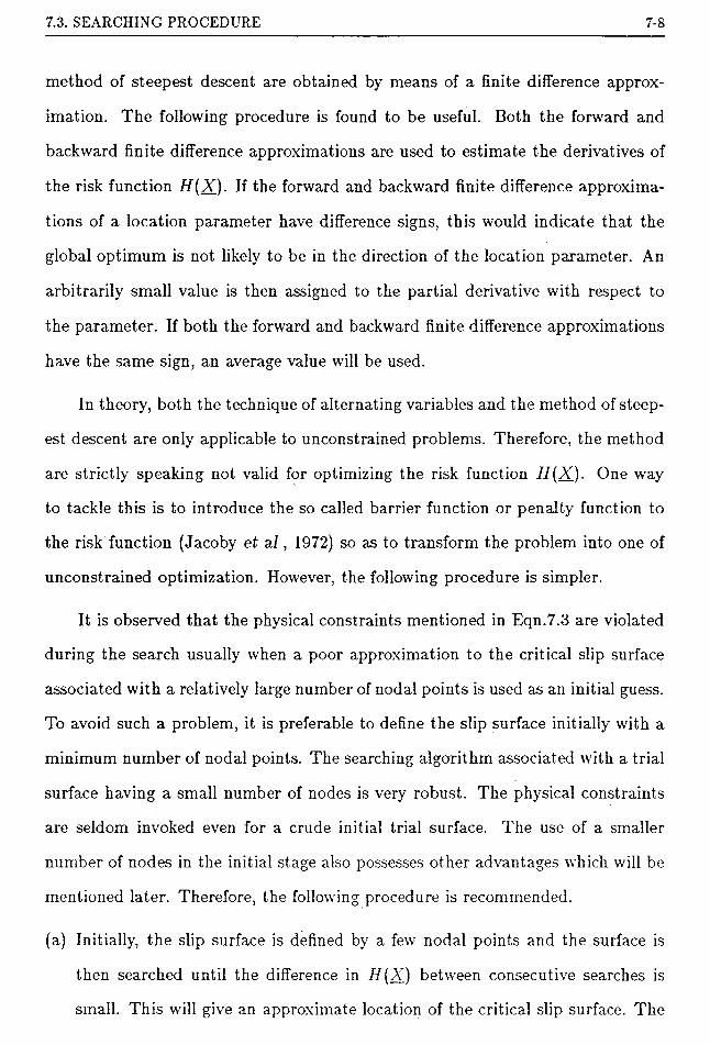
7.3. SEARCHING PROCEDURE 7-8
method of steepest descent are obtained by means of a finite difference approx
imation. The following procedure is found to be useful. Both the forward and
backward finite difference approximations are used to estimate the derivatives of
the risk function H()Q- If the forward and backward finite difference approxima
tions of a location parameter have difference signs, this would indicate that the
global optimum is not likely to be in the direction of the location parameter. An
arbitrarily small value is then assigned to the partial derivative with respect to
the parameter. If both the forward and backward finite difference approximations
have the same sign, an average value will be used.
In theory, both the technique of alternating variables and the method of steep
est descent are only applicable to unconstrained problems. Therefore, the method
are strictly speaking not valid for optimizing the risk function H(X). One way
to tackle this is to introduce the so called barrier function or penalty function to
the risk function (Jacoby et al , 1972) so as to transform the problem into one of
unconstrained optimization. However, the following procedure is simpler.
It is observed that the physical constraints mentioned in Eqn.7.3 are violated
during the search usually when a poor approximation to the critical slip surface
associated with a relatively large number of nodal points is used as an initial guess.
To avoid such a problem, it is preferable to define the slip surface initially with a
minimum number of nodal points. The searching algorithm associated with a trial
surface having a small number of nodes is very robust. The physical constraints
are seldom invoked even for a crude initial trial surface. The use of a smaller
number of nodes in the initial stage also possesses other advantages which will be
mentioned later. Therefore, the following procedure is recommended.
(a) Initially, the slip surface is defined by a few nodal points and the surface is
then searched until the difference in //(X) between consecutive searches is
small. This will give an approximate location of the critical slip surface. The

7.3. SEARCHING PROCEDURE 7-9
tolerance can be less stringent at the begining.
(b) New nodal points are then introduced automatically at the mid-point of the
straight line joining adjacent nodes of this approximate critical slip surface.
The slip surface, which is now refined by more nodal points, is searched until
the required accuracy is attained.
(c) Step (b) is repeated until the addition of more nodal points does not result in
any appreciable change in the value of H(X_).
To avoid premature termination of the search in step (a) or (b), the following
termination criterion is suggested. If the difference in the value of H(X_) for three
successive searches, is smaller than the tolerance, this step can be terminated.
Provided that a reasonable initial estimate of the critical slip surface is present,
as is obtained by searching a slip surface having a small number of nodes in this
case, the physical constraints of the location parameters are seldom invoked during
subsequent refinements of the slip surface.
There is no guarantee that the above procedure will not violate the constraints
during the search. Consider more closely the constraints in Eqn.7.3. When the
constraints are violated, it simply means that two adjacent nodal points are ap
proaching each other, trying to cross one another. It indicates that the slip surface
is ‘over-specified’ by having too many nodal points. A simple solution to solve this
problem is to remove one of the two points which is causing the trouble. The
algorithm is restarted with the slip surface now defined with fewer nodal points.
Such a procedure is found to be successful.
For circular slip surfaces, the treatment is much simpler. Normally the only
likely constraint will be on the radius of the slip circle. In such cases, the radius
can usually be expressed in terms of the center of the slip circle. As a result,
the risk function will become a function of two variables and there is usually
no further constraints for this transformed function except perhaps that the slip
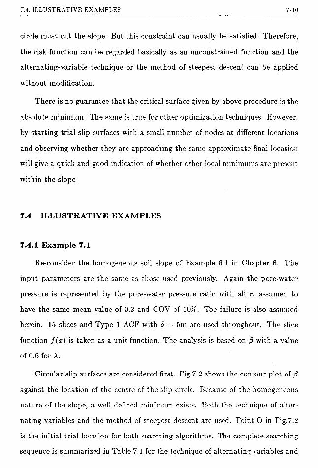
7.4. ILLUSTRATIVE EXAMPLES 7-10
circle must cut the slope. But this constraint can usually be satisfied. Therefore,
the risk function can be regarded basically as an unconstrained function and the
alternating-variable technique or the method of steepest descent can be applied
without modification.
There is no guarantee that the critical surface given by above procedure is the
absolute minimum. The same is true for other optimization techniques. However,
by starting trial slip surfaces w:ith a small number of nodes at different locations
and observing whether they are approaching the same approximate final location
will give a quick and good indication of whether other local minimums are present
within the slope
7.4 ILLUSTRATIVE EXAMPLES
7.4.1 Example 7.1
Re-consider the homogeneous soil slope of Example 6.1 in Chapter 6. The
input parameters are the same as those used previously. Again the pore-water
pressure is represented by the pore-water pressure ratio with all rx assumed to
have the same mean value of 0.2 and COV of 10%. Toe failure is also assumed
herein. 15 slices and Type 1 ACF with b — 5m are used throughout. The slice
function f(x) is taken as a unit function. The analysis is based on (3 with a value
of 0.6 for A.
Circular slip surfaces are considered first. Fig.7.2 shows the contour plot of (3
against the location of the centre of the slip circle. Because of the homogeneous
nature of the slope, a well defined minimum exists. Both the technique of alter
nating variables and the method of steepest descent are used. Point O in Fig.7.2
is the initial trial location for both searching algorithms. The complete searching
sequence is summarized in Table 7.1 for the technique of alternating variables and

7.4. ILLUSTRATIVE EXAMPLES 7-11
cP Y<r
non- feasibleregion
x-axis (m)
Figure 7.2 Contour Plot of /3 - Example 7.1
- axi
s (m
)

7.4. ILLUSTRATIVE EXAMPLES 7-12
Point Centre p accs accg
O (0.00,15.00) 3.96 - -
A (-2.14, 15.00) 3.47 0.01 0.1
B (-2.14, 14.86) 3.47 0.01 0.1
C (-2.10,14.86) 3.47 0.01 0.1
D (-2.10, 14.75) 3.47 0.01 0.1
E (-2.10, 14.75) 3.47 0.0001 0.01
F (-2.10, 14.68) 3.46 0.0001 0.01
G (-2.03, 14.68) 3.46 0.0001 0.01
N (-2.04, 14.65) 3.46 0.0001 0.01
Table 7.1.
Searching Sequences for Circular Slip Surface - Example 7.1
(Alternating-variable technique)

7.4. ILLUSTRATIVE EXAMPLES 7-13
Point Centre 0 accs accg
0 (0.00,15.00) 3.95 - -
A' (-1.65, 14.23) 3.46 0.01 0.1
B' (-1.69,14.19) 3.46 0.01 0.1
C (-1.65,14.24) 3.45 0.01 0.1
D' (-1.70, 14.20) 3.46 0.01 0.1
E' (-1.70, 14.21) 3.45 0.0001 0.01
F' (-1.70, 14.21) 3.45 0.0001 0.01
G' (-1.70, 14.21) 3.45 0.0001 0.01
H' (-1.70, 14.21) 3.45 0.0001 0.01
N' (-1.70,14.21) 3.45 0.0001 0.01
Table 7.2.
Searching Sequences for Circular Slip Surface - Example 7.1
(Method of Steepest Descent)
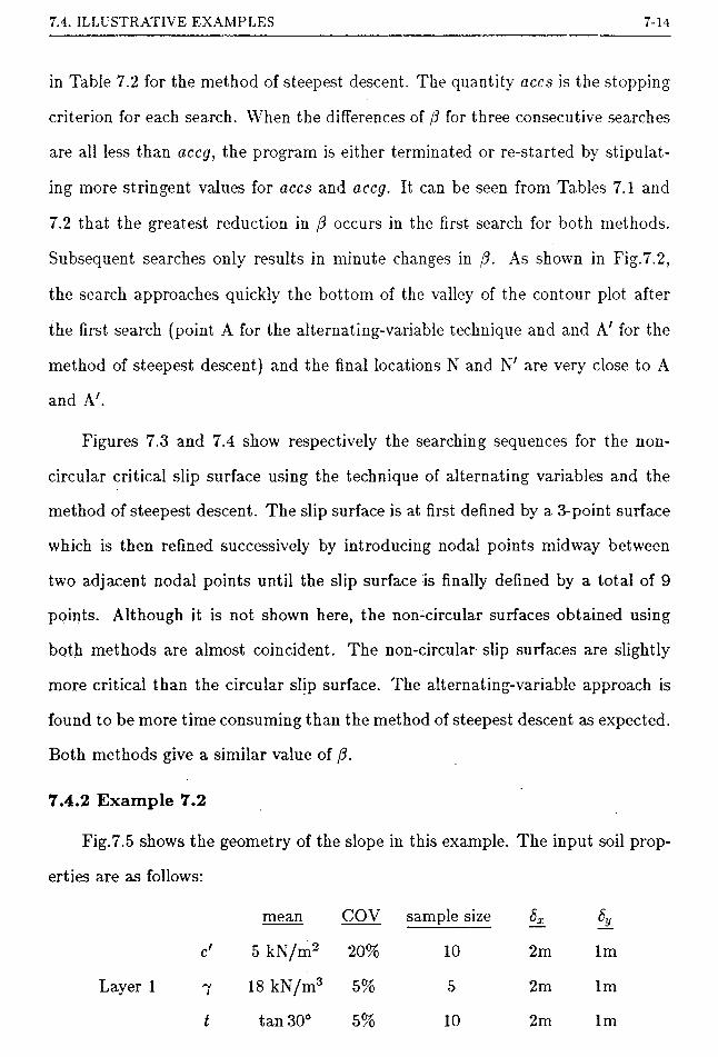
7.4. ILLUSTRATIVE EXAMPLES 7-14
in Table 7.2 for the method of steepest descent. The quantity accs is the stopping
criterion for each search. When the differences of p for three consecutive searches
are all less than accg, the program is either terminated or re-started by stipulat
ing more stringent values for accs and accg. It can be seen from Tables 7.1 and
7.2 that the greatest reduction in p occurs in the first search for both methods.
Subsequent searches only results in minute changes in 3. As shown in Fig.7.2,
the search approaches quickly the bottom of the valley of the contour plot after
the first search (point A for the alternating-variable technique and and A' for the
method of steepest descent) and the final locations N and N7 are very close to A
and A'.
Figures 7.3 and 7.4 show respectively the searching sequences for the non-
circular critical slip surface using the technique of alternating variables and the
method of steepest descent. The slip surface is at first defined by a 3-point surface
which is then refined successively by introducing nodal points midway between
two adjacent nodal points until the slip surface is finally defined by a total of 9
points. Although it is not shown here, the non-circular surfaces obtained using
both methods are almost coincident. The non-circular slip surfaces are slightly
more critical than the circular slip surface. The alternating-variable approach is
found to be more time consuming than the method of steepest descent as expected.
Both methods give a similar value of /?.
7.4.2 Example 7.2
Fig.7.5 shows the geometry of the slope in this example. The input soil prop
erties are as follows:
mean COV sample size k
c' 5 kN/m2 20% 10 2 m lm
Layer 1 7 18 kN/m3 5% 5 2 m lm
t tan 30° 5% 10 2m lm

rem
arks
7.4. ILLUSTRATIVE EXAMPLES 7-15
o o o
p Oo o
• --- 4-< '.tr CL CL Ql
rn cn
“D
£cna>
l—
a>&
Sear
ch fo
r Non
-circ
ular
Slip
S

emar
k
7.4. ILLUSTRATIVE EXAMPLES 7-16
h-OG*
t-<Dt-3bp
U-t
Sear
ch fo
r Non
-circ
ular
Slip
Surf
ace -
Exa

7.4. ILLUSTRATIVE EXAMPLES 7-17

7.4. ILLUSTRATIVE EXAMPLES 7-18
mean cov sample size 6*
c' 10 kN/m2 20% 8 2 m 2 m
Layer 2 7 18 kN/m3 5% 5 2m 2 m
t tan 30° 5% 8 2 m 2m
The pore-water pressure is descrbed using the second model described in Sec
tion 6.6. The curves yu(x), Vp(j) and iji(x) represent respectively the upper bound,
most probable level and lower bound of the phreatic surface. Other details of an
alysis are the same as Example 7.1.
Circular slip surfaces are considered first. Fig.7.6 shows the contour plot
of (3 against the location of the centre of the slip circle. It can be seen that
multiple local minimums exist as would be expected for non-homogeneous slopes.
To locate the absolute minimum, the search process has to be started at different
initial positions. Fig.7.6 shows two search sequences started at two different, initial
locations (points O and O' in the figure). The method of steepest descent is used.
Points A and A' in the figure represent the positions after the first descent with
accs set at 0.01. The search is then continued until the difference in /3 between
three consecutive searches are all less than 0.1. The search is then re-started with
accs set at 0.001 and accg set at 0.01. The final position of the search is marked
as points N (3 = 4.14) and N' (3 = 4.26). in the figure. It can be seen that
the greatest reduction of (3 occurs during the first descent. The search quickly
approaches the minimum point after the very first descent. Once the minimum
location is near, subsequent searches will only result in minute changes of (3 and
locations of the centres of the slip circles.
Fig.7.7 shows the results for non-circular slip surface. Both the technique of
alternating variables and the method of steepest descent are used.

7.4. ILLUSTRATIVE EXAMPLES 7-19
17
- 16
15
14
12-5 -4 -3
x -axis (m)
Figure 7.6Contour Plot of {3 Against Center of Slip Circle - Example 7.2
- axi
s (m
)

lege
nd
rem
arks
7.4. ILLUSTRATIVE EXAMPLES 7-20

7.4. ILLUSTRATIVE EXAMPLES 7-21
At first, the slip surface is defined by two straight lines having three nodal
points as shown in the figure. The 3-point critical slip surface is located. The
slip surface is then refined by introducing nodal points mid-way between the two
straight lines. The slip surface, now defined by five nodal points, is again searched.
The process is repeated until the slip surface is finally defined by 9 nodal points for
the alternating-variable technique and 8 nodal points for the method of steepest
descent (one point has been deleted as two of the points are too close together
during the search). The final values of accg is set at 0.01. The alternating-variable
technique gives a slightly more critical slip surface with a smaller value of fl.
In slope stability analysis, a critical band near the critical slip surface can
usually be found. All slip surfaces within this band would have factor of safety,
reliability index or failure probability very close to that of the critical slip surface.
This is demonstrated by the results shown in Fig.7.7. Although the slip surfaces
obtained using the two methods are some distance apart, the numerical difference
of (5 is less than 59o indicating that these two surfaces are within or close to the
critical band.

CHAPTER 8
LIMITATIONS AND SUGGESTIONS
This thesis has presented a general probabilistic approach to slope design.
However, the discussion will not be complete without mentioning the limitations
of the present approach and pointing out some of the areas where further research
would be necessary.
1. A two-dimensional stability model is used herein. This is equivalent to saying
that soil properties are perfectly correlated in the transverse direction. The
consequence of such an assumption remains a question of further inquiry. But
no doubt a three-dimensional analysis, especially for c-0 slopes, will be much
more complicated than a two-dimensional analysis both in terms of the formu
lation of the performance function and the generation of the covariance matrix
of the spatial average soil properties. No detailed probabilistic study on three-
dimensional soil slopes has yet been published in the literature for c-^> slopes,
although attempts have been made to analyze a three-dimensional 0 = 0 slope
using a level-crossing approach (Yanmarcke, 1977bYl980; Yeneziano and An-
toniano, 1979).
2. Model uncertainty and measurement errors of soil properties have not been
considered. The failure probability given by the present model will therefore
be the lower bound values. Given the statistical properties of the model un
certainty and the measurement erros, the procedure for incorporating these
uncertainties into the analysis is relatively straight forward (see e.g. Yuceman
8-1

8. LIMITATIONS AND SUGGESTIONS 8-2
et a1 ,1973; and Ang and Tang, 1984). Of course, the questions are how to
calibrate the accuracy of the limit equilibrium method and to determine the
testing errors of soil measurements. These questions cannot be answered solely
by the use of statistics. A better understanding of the physics of the problem
and the fundamental concepts of soil mechanics is necessary.
3. In a limit equilibrium analysis, soils are assumed to be perfectly plastic mate
rials. On this basis, the spatially averaged soil properties will be the pertinent
parameters to use in the analysis. However, for strain-softening soils, the ef
fect of ‘brittle’ failure cannot be overlooked. In a conventional deterministic
analysis in which the soil properties are assumed to be constant, the yield zone
always initiates at the location with the highest stress level. However, the pic
ture will be somewhat different when looked at from a probabilistic point of
view. Since soil properties van' from point to point within a slope, there may
be a chance that the soil strength is very low at a location where the stress
level is not the highest. Failure can well initiate from this point instead of the
most highly stressed region. On the other hand, if it so happens that the soil
strength is the lowest at the most highly stressed region, the yield zone may
propagate catastrophically to the adjoining area leading to a sudden failure of
slope.
The spatial variability of soil has therefore two opposing consequences. On
the one hand, the spatial variability reduces the variance of the average soil
properties and hence the failure probability of slopes. On the other hand,
spatial variability of soil will increase the likelihood of progressive failure as
failure can initiate at any location along the slip surface. Which effect will
dominate depends on the strain-softening behaviour of soil, at present study
on this topic is limited. Further discussion is given in Tang et al (1985).
4. The system reliability of failure probability of slopes remains a relatively ‘unde-
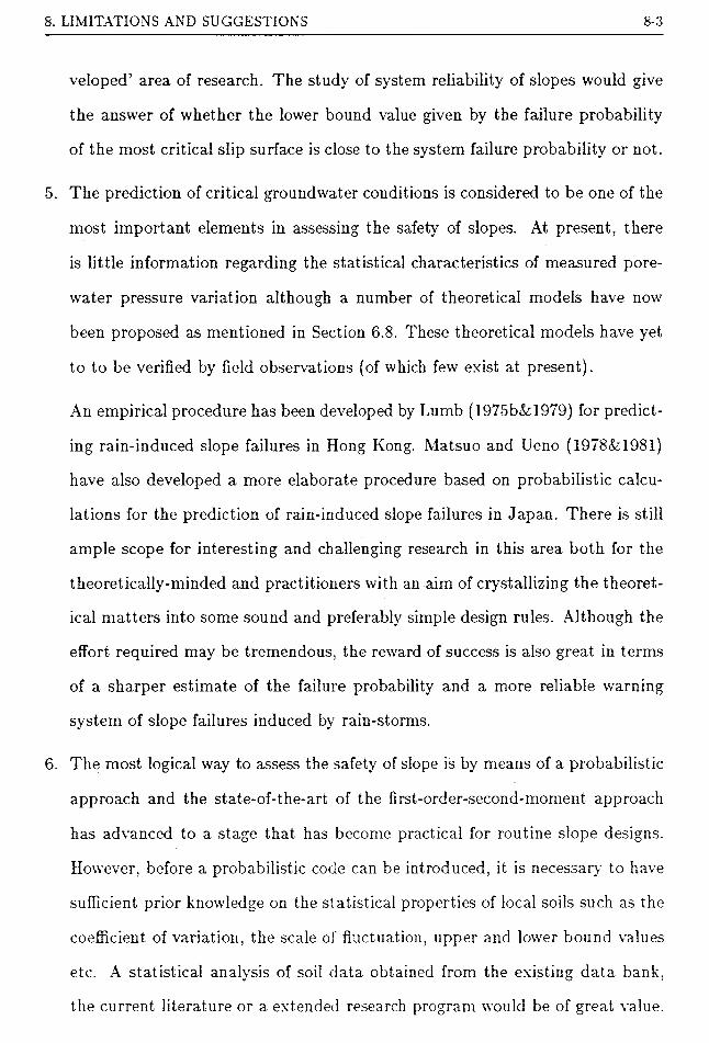
8. LIMITATIONS AND SUGGESTIONS 8-3
velopecP area of research. The study of system reliability of slopes would give
the answer of whether the low’er bound value given by the failure probability
of the most critical slip surface is close to the system failure probability or not.
5. The prediction of critical groundwater conditions is considered to be one of the
most important elements in assessing the safety of slopes. At present, there
is little information regarding the statistical characteristics of measured pore-
water pressure variation although a number of theoretical models have now
been proposed as mentioned in Section 6.8. These theoretical models have yet
to to be verified by field observations (of which few exist at present).
An empirical procedure has been developed by Lumb (1975b&1979) for predict
ing rain-induced slope failures in Hong Kong. Matsuo and Ueno (1978&T981)
have also developed a more elaborate procedure based on probabilistic calcu
lations for the prediction of rain-induced slope failures in Japan. There is still
ample scope for interesting and challenging research in this area both for the
theoretically-minded and practitioners with an aim of crystallizing the theoret
ical matters into some sound and preferably simple design rules. Although the
effort required may be tremendous, the reward of success is also great in terms
of a sharper estimate of the failure probability and a more reliable warning
system of slope failures induced by rain-storms.
6. The most logical way to assess the safety of slope is by means of a probabilistic
approach and the state-of-the-art of the first-order-second-moment approach
has advanced to a stage that has become practical for routine slope designs.
However, before a probabilistic code can be introduced, it is necessary to have
sufficient prior knowledge on the statistical properties of local soils such as the
coefficient of variation, the scale of fluctuation, upper and lower bound values
etc. A statistical analysis of soil data obtained from the existing data bank,
the current literature or a extended research program would be of great value.

8. LIMITATIONS AND SUGGESTIONS 8-4
Further studies on the cross-correlation of soil properties and the simplification
of the structural analysis of a Type III soil profile would also be useful.

CHAPTER 9
CONCLUSIONS
A general probabilistic approach to slope design using the random field model
and Morgenstern and Price's method is presented. This study utilizes a rigorous
model for the formulation of the performance function. By following the unified
solution scheme discussed in Chapter 3, this approach has the potential to be
extended to other rigorous stability models currently in use in the literature. An
other salient feature of the scheme is that the performance function can be defined
explicitly in terms of the basic random variables with no need of iteration for the
calculation of the interslice forces, thus enabling the derivatives of the performance
function to be evaluated analytically.
Formulating the performance function as a safety margin has the advantage of
minimizing the non-linearity of the function. This results in fast convergence for
the calculation of the reliability index Phl and simplifies greatly the calculation
of the lower and upper bounds of the performance function. The use of a safety
margin also makes the assumption of normal distribution for the performance
function more reasonable by virtue of the central limit theorem.
The random field model has been extended to cover non-homogeneous soil
profiles and take account of the sampling uncertainty. A series of useful formulae
is developed to facilitate the calculation of the variances and covariances of the
spatially averaged soil properties.
The state-of-the-art of the structural analysis of soil data is also critically
9-1
9. CONCLUSIONS 9-2
reviewed. It is considered that more research should be carried out to establish
some practical yet sound procedures for the estimation of the statistical properties
of soils.
Comparisons are made for different probabilistic approaches to slope design,
namely the approaches based on ;3, 3hl and PDF fitting. Studies indicate that
the reliability index ,3hl is essentially identical to the reliability index (3 when the
performance function is formulated as a safety margin. This can be attributed to
the fact that the performance function so formulated is ‘almost' linear.
Experience indicates that at a high level of failure probability (> 10~2 - 10-3),
the values of Pf inferred from all the above three methods are similar. However,
a larger difference exists between the value obtained from PDF fitting and those
from the reliability indices (3 or (3hl when the failure probability is small.
It is also observed that the failure probability based on Gm(X) is much less
sensitive to the parameter A than that based on Gj(X). Although the use of a
rigorous solution is always desirable, an approximate result based only on Gm(X)
and a reasonable value of A would very often give a sufficiently accurate answer.
Results also show that the failure probability of slopes is not sensitive to
the types of interslice force functions and autocorrelation functions. However,
it depends significantly on the magnitude of the scales of fluctuation which are
considered to be the most important parameter that characterizes the correlation
structure of soil properties. More attention should be paid to the estimation of
this parameter than has hitherto been the case.
An algorithm for locating the critical slip surface is developed. The critical
surface with minimum factor of safety very often gives a good indication of the
likely location of the critical surface with maximum failure probability.
Although there are still problems to be solved regarding the probabilistic mod
elling of soil behaviour, variation of pore-water pressure and the methodology for
9. CONCLUSIONS 9-3
reliability calculations, it is pedantic to delay the use of the available probabilis
tic methods, especially the FOSM approach, for want of a completely rigorous
analysis. The main advantage of using a probabilistic approach is to provide an
operational procedure by which the uncertainties of the design can be considered.
It also helps the engineer to quantify experience by building up knowledge on
the values of the statistical parameters such as the COV or scales of fluctuation
of local soils. These judgemental values can always be updated and uncertain
ties sharpened when more information becomes available. Moreover, experience
is more easily transmitted to an inexperienced engineer by conveying the likely
values of the statistical properties of the soil than just specifying a magic number
for the factor of safety.
REFERENCES
Abramowitz,M. and Stegun,I.A.(Eds)(1970) Handbook of Mathematical Functions, Dover Publication, New York, 1045pp.
Agterberg,F.P.( 1967) ‘Mathematical Models in Ore Evaluation’, Journal of Canadian Operational Research Society, Vol.5, ppl44-158.
Agterberg,F.P.( 1974) Geomathematics - Mathematical Background and Geoscience Applications, Elsevier Scientific Publishing Co., Amsterdam, 59Gpp.
Alonso,E.E.( 1976) ‘Risk Analysis of Slopes and its Application to Slopes in Canadian Sensitive Clays’, Geotechnique, Vol.26, pp453-472.
Alonso,E.E. and Krizek,R.J.( 1975) ‘Stochastic Formulation of Soil Properties’, Proc. 2nd International Conference on Applications of Statistics and Probability to Soil and Structural Engineering, Aachen, pp9-32.
Anderson,M.G. and Howes,S.(1985) ‘Development and Application of a Combined Soil Water-Slope Stability Model’, Quarterly Journal of Engineering Geology, Vol.18, pp225-236.
Anderson,L.R., Bowles,D.S., Canfield,R.V. and Sharp,K.D.( 1982) Probabilistic Modeling of Tailings Embankment Designs, Vol.l: Model Development and Verification, Bureau of Mines, U.S.A., 231pp.
Andersson,J. and Shapiro,A.M.( 1983) ‘Stochastic Analysis of One-dimensional Steady State Unsaturated Flow: A Comparison of Morte Carlo and Perturbation Methods’, Water Resources Research, Vol.19, No.l, pp 121-131.
Ang,A.H.S. and Tang, W.H.( 1984) ‘Probability Concepts in Engineering Planning and Design’, Vol.2, Decision, Risk, and Reliability, John Wiley and Sons, New York, 562pp
Arnold,S.F.( 1981) The Theory of Linear Models and Multivariate Analysis, John Wiley and Sons, New York, 475pp.
Asaoka,A. and Grivas,D.A.(1982) ‘Spatial Variability of the Undrained Strength
R-l
REFERENCES R-2
of Clays’, Journal Geotechnical Engineering Division, ASCE, Vol.108, No.GTo, pp743-756.
Baecher,G.B.( 1984) ‘Need for Probabilistic Characterization (Just a Few More Tests and We’ll be Sure!)’, Probabilistic Characterization of Soil Properties: Bridge Between Theory and Practice, (Eds) D.S. Bowles and H.Y. Ko, ASCE, ppl-18.
Baecher,G.B., Chan,M., Ingra,T.S., Lee,T., and Nucci,L.R.( 1980) Geotechnical Reliability of Offshore Gravity Platforms, Report No. MITSG 80-20, M.I.T., Cambridge, Mass., 291pp.
Beacher,G.B., Einstein,H.H., Vanmarcke,E.H., Veneziano,D. and Whitman,R.V. (1984) Discussion on ‘Conventional and Probabilistic Embankment Design’, by V. McGuffey et al (1982), Journal of Geotechnical Engineering Division, ASCE, Vol.110, No.GT7, pp989-991.
Baker,R.(1980) ‘Determination of the Critical Slip Surface in Slope Stability Computations’, International Journal for Numerical and Analytical Methods in Ge- omechanics, Vol.4, pp333-359.
Baker,R. and Garber,M.( 1977a) Discussion on ‘On Slip Surface and Slope Stability Analysis’ by Chen,W.F. and Snitbhan,N.S., Soils and Foundations, Vol.17, pp65-68.
Baker,R. and Garber,M.( 1977b) ‘Variational Approach to Slope Stability’, Proceedings 9th International Conference on Soil Mechanics and Foundation Engineering, Tokyo, Vol.2, pp9-12.
Baker,R. and Garber,M.( 1978) ‘Theoretical Analysis of the Stability of Slopes’, Geotechnique, Vol.28, pp395-411.
Bao,C.G. and Yu,L.(1985) ‘Probabilistic Method for Analyzing the Stability of Slope under Special Conditions (in Chinese)’, paper presented in the Conference on Strength and Constitutive Relation of Soils, Wunan.
Bai tlett,M.S.(1946) ‘On the Theoretical Specification and Sampling Properties of Autocorrelated Time-Series’, Supplement - Journal of Royal Statistical Society, Vol.8, No.27, pp24-41.
Bell,J.M.( 1968) ‘General Slope Stability Analysis’, Journal of Soil Mechanics and Foundations Division, ASCE, Yol.94, No.SMC, pp 1253-1270.
Bell,J.M.(1969) ‘Non-circular Sliding Surfaces’, Journal of Soil Mechanics and Foundations Division, ASCE, Vol.95, No.SM3, pp829-844.
Benjamin,J.R. and Cornell,C.A.(1970) Probability, Statistics and Decision For Civil Engineers, McGraw Hill Book Co., New York, 684pp.
Bennet,R.J.( 1979) Spatial Time Series : Analysis - Forecasting - Control, Pion

REFERENCES R-3
Limited, London, 674pp.
Bergado.D.T. and Anderson.L.R.( 1985) ‘Stochastic Analysis of Pore-pressure Uncertainty for the Probabilistic Assessment of the Safety of Earth Slopes’, Soils and Foundations, Vol.25, No.2, pp87-105.
Beveridge.G.S.G. and Schechter,R.S.( 1970) Optimization: Theory and Practice, McGraw Hill Book Co., New York, 773pp.
Biernatowski.K.f 1969) ‘Stability of Slope in Probabilistic Solution’, Proc. 7th International Conference on Soil Mechanics and Foundation Engineering, Mexico, Vol.2, pp527-530.
Biernatowski,K.( 1976) ‘Stability of Slopes in Variational and Probabilistic Solutions’, Proc. 6th European Conference on Soil Mechanics and Foundation Engineering, Vol.l, pp3-7.
Biernatowski,K.( 1979) ‘Margin of Safety for Slope Stability’, Proc. 3rd International Conference on Applications of Statistics and Probability in Soil and Structural Engineering, Sydney, Vol.2, pp431-436.
Biernatowski,I\.( 1987) ‘Stability and Safety Measures of Slopes in Probabilistic Formulation’, Proc. 5th International Conference on Applications of Statistics and Probability in Soil and Structural Engineering, Vancouver, Vol.2, pp853- 858.
Bishop,A. W.( 1955) ‘The Use of the Slip Circle in the Stability Analysis of Slopes’, Geotechnique, Vol.5, pp7-17.
Bolotin, V.V.( 1973) Statistical Met hods in Structural Mechanics, Holden-Day, 240pp.
Boutrup,E. and Lovell,C.\V.(1980) ‘Searching Techniques in Slope Stability Analysis’, Engineering Geology, Vol.lS, pp51-61.
Brand,E.W., Dale,M.J. and Nash,.I.M.(1986) ‘Soil Pipes and Slope Stability in Hong Kong’, Quarterly Journal of Engineering Geology, Vol.19, pp301-303.
Castillo,E. and Alonso,E.E.( 1985) ‘Probabilistic Versus Deterministic Modelling : Filling a Gap’, Proc. 11th International Conference on Soil Mechanics and Foundation Engineering, San Francisco, Vol.2, pp813-818.
Castillo.E. and Revilla,J.(1977) ‘The Calculus of Variations and the Stability of Slopes’, Proceeding 9th International Conference on Soil Mechanics and Foundation Engineering, Tokyo, Vol.2, pp25-30.
Chang.C.S. and Soong,T.T.( 1979) ‘A Probabilistic Approach to Consolidation Analysis’, Proc. 3rd International Conference on Applications of Statistics and Probability on Soil and Structural Engineering, Sydney, Vol.2, pp487-496.
Celestino.T.B. and Duncan,J.M.( 1981) ‘Simplified Search for Noncircular Slip Sur-

REFERENCES R-4
faces’, Proceeding 10th International Conference on Soil Mechanics and Foundation Engineering, Stockholm, Sweden, pp391-394.
Chen, W.F.( 1975) Limit Analysis and Soil Plasticity, Elsevier Scientific Publishing Company, Amsterdam, 638pp.
Chen,X. and Lind,N.C.(1983) ‘Fast Probability Integration by Three-Parameter Normal Tail Approximation’, Structural Safety, Vol.l, pp269-276.
Cheong,II.F. and Subrahmanyam,R.V.(1983) ‘Slope Failure Probabilities Based on Taylor’s Analysis’, Journal of the Institution of Engineers, India, C.E.Div., Vol.63, No.5, pp252-258.
Chirlin,G.R. and Dagan,G.( 1980) ‘Theoretical Head Variograms for Steady Flow in Statistically Homogeneous Aquifers’, Water Resources Research, Vol.16, No.6, ppl001-1015.
Chowdhury,R.N.( 1981) Probabilistic Approaches to Progressive Failure, First Report, University of Wollongong.
Chowdhury,R.N.( 198-1) ‘Recent Developments in Landslide Studies: Probabilistic Methods - State-of-the-Art Report’, 4th International Symposium on Landslides, Toronto, Canada, Vol.l, pp209-228.
Chowdhury,R.N. and Deroy,E.R.( 1985) ‘Progressive Reliability of a Strain Softening Slope’, Civil Engineering Transaction, I.E.Aust., Vol.CE27, No.l, pp79-94.
Christakos,G.( 1984) ‘On the Problem of Permissible Covariance and Variogram Models’, Water Resources Research, Vol.20, No.2, pp251-265.
Clark,1.(1979) Practical Geostatistics, Applied Science Publishers Ltd., London, 129pp.
Cody,W.J.( 1969) ‘Rational Chebyshev Approximations for the Error Function’, Mathematics of Computation, Vol.23, pp631-637.
Cornell,C.A.(1967) ‘Bounds on the Reliability of Structural Systems’, Journal Structural Division, ASCE, Vol.93, No.STl, ppl71-200.
Cornell,C.A.(1969) ‘A Probability-based Structural Code’, Journal of American Concrete Institute, Vol.66, No. 12, pp974-985.
Cornell,C.A.(1971) ‘First-order Uncertainty Analysis of Soils Deformation and Stability’, Proc. 1st International Conference on Applications of Statistics and Probability in Soil and Structural Engineering, Hong Kong, ppl29-144.
Cox,N.D.(1979) ‘Tolerance Analysis by Computer’, Journal of Quality Technology', Vol.l 1, No.2, pp80-87.
Cremer,IL(1946) Mathematical Methods of Statistics, Cambridge University Press,

REFERENCES R-5
Cressie,N.(1979) ‘Straight Line Fitting and Variogram Estimation’, Bulletin of the International Statistical Institute, Vol.48, pp573-576.
Cressie,N.( 1983) ‘Towards Resistant Geostatistics’, Geostatistics for Natural Resources Characterization, (Eds) G. Verly et al, D. Reidal Publishing Co., part 1, pp21-44.
Cressie,N.( 1985) ‘Fitting Variogram Models by Weighted Least Squares’, Mathematical Geology, Vol.17, No.5, pp563-586.
Cressie,N. and Glonek,G.( 1984) ‘Median Based Covariogram Estimators Reduce Bias’, Statistics and Probability Letters, Vol.2, pp299-304.
Cressie,N. and Hawkins,D.M.( 1984) ‘Robust Estimation of the Variogram: I’, Mathematical Geology, Vol.12, No.2, ppl 15-125.
David,M.( 1977) Geostatistical Ore Reserve Estimation, Elsevier Scientific Publishing Co., Amsterdam, 364pp.
Davis,P.J. and Rabinowitz,P.( 1975) Methods of Numerical Integration, Academic Press, New York, 459pp.
Delfiner,P.(1976) ‘Linear Estimation of Non Stationary Spatial Phenomena’, Advanced Geostatistics in the Mining Industry, (Ed.) M. Guarascio et a I, pp49-68.
Der I\iureghian,A. and Liu,P-L.( 1986) ‘Structural Reliability LTnder Incomplete Probability Information’, Jounral of Engineering Mechanics, ASCE, Vol.112, pp85-104.
Ditlevsen,0.( 1981) ‘Principle of Normal Tail Approximation’, Journal of Engineering Mechanics Division, ASCE, Vol.107, ppl 191-1208.
Ditlevsen,0.( 1983) ‘Gaussian Safety Margins’, Proc. 4th International Conference on Applications of Statistics and Probability in Soil and Structural Engineering, Italy, pp785-824.
Dowd,P.A.(1983) ‘The Variogram and Kriging- Robust and Resistant Estimators’, Geostatistics for Natural Resources Characterization, (Eds) G. Verly et a/, part 1, pp91-106.
Draper,N.R. and Smith,H.(1981) Applied Regression Analysis, John Wiley and Sons, New York, 709pp.
Duncan,J.M. and Wright,S.G.( 1980) ‘The Accuracy of Equilibrium Methods of Slope Stability Analysis’, Quarterly Journal of Engineering Geology, Vol.16, pp5-17.
Edil,T.B. and Shultz,M.N.(1982) ‘Landslide Hazard Potential Determination Along a Shoreline Segment’, Engineering Geology, Vol.19, ppl59-177.
Elderton,W.P. and Johnson,N.L.( 1969) Systems of Frequency Curves, Cambridge

REFERENCES R-6
University Press, Cambridge, 216pp.
Evans,D.H.( 1967) ‘An Application of Numerical Integration Technique to Statistical Tolerancing’, Technometrics, Vol.9, pp441-456.
Evans,D.H.( 1972) ‘An Application of Numerical Integration Technique to Statistical Tolerancing III - General Distributions’, Technometrics, Vol.14, pp25-35.
Fardis,M.N. and Veneziano,D.(1981) ‘Estimation of SPT-N and Relative Density’, Journal Geotechnical Engineering Division, ASCE, Vol.107, No.GTlO, ppl345- 1359.
Felio,G.Y., Lytton,R.L. and Briaud,J.L.(1984) ‘Statistical Approach to Bishop’s Method of Slices’, International Symposium on Landslides, Toronto, Vol.2,pp411-415.
Fiessler,B., Neumann,H.J. and Rackwitz,R.(1979) ‘Quadratic Limit States in Structural Reliability’, Journal of Engineering Mechanics Division, ASCE, Vol.105, pp661-676.
Forster, VV. and Weber,E.( 1981) ‘Influences on the Probability of Failure of Slopes’, Proc. 10th International Conference on soil Mechanics and Foundation Engineering, Vol.l, ppl27-130.
Fredlund,D.G. and Krahn,J.( 1976) ‘Comparison of Slope Stability Methods of Analysis’, Proc. 29th Canadian Geotechnical Conference - Slope Stability, The Canadian Geotechnical Society, Pt.VIII, pp57-74.
Gao,D.(1985) ‘Reliability Analysis and Evaluation of Soil-Property Parameters (in Chinese)’, Journal of Tongji University, No.4, pp59-68.
Garber,M.D.( 1973) ‘Variational Method for Investigating the Stability of Slopes’, Soil Mechanics and Foundation Engineering, Vol.10, pp77-79.
Geary,R.C.( 1930) ‘The Frequency Distribution of the Quotient of Two Normal Variates’, Journal of Royal Statistical Society, Vol.93, pp442-446.
Ghiocel,D. and Lungu,D.(1975) Wind, Snow and Temperature Effects on Structures Based on Probability, Abacus Press, Kent, 411pp.
Goni,J.J. and Hadj-Hamou,T.( 1987) ‘Application of Number Theoretic Methods to the Reliability Analysis of a Gravity Retaining Wall’, Proc. 5th International Conference on Applications of Statistics and Probability in Soil and Structural Engineering, Vancouver, Vol.2, pp678-685.
Grigoriu,M.( 1983a) ‘Approximate Analysis of Complex Reliability Problems’, Structural Safety, Vol.l, pp277-288.
Grigoriu,M.( 1983b) ‘Approximate Reliability Analysis’, Recent Advances in Engineering Mechanics and Their Impart on Civil Engineering Practice, (Ed) W.F.
REFERENCES R-7
Chen and A.D.M. Lewis, Vol.2, pp867-870.
Grigoriu,M. and Lind,N.C.(1980) ‘Optimal Estimation of Convolution Integrals’, Journal of Engineering Mechanics Division, ASCE, Vol.106, N0.EM6, ppl349- 1364.
Grivas,D.A.(1979) ‘Reliability Analysis of Retaining Structures’, Proc. 3rd International Conference on Applications of Statistics and Probability on Soil and Structural Engineering, Sydney, Vol.2, pp632-641.
Grivas,D.A.(1981) ‘How Reliable Are Present Methods of Slope Failure Prediction?’, Proc. 10th International Conference on Soil Mechanics and Foundation Engineering, Stockholm, Vol.3, pp427-430.
Grivas,D.A. and Harr,M.E.(1977) ‘Reliability With Respect to Bearing Capacity Failures of Structures on Ground’, Proc. Specialty Session, 9th International Conference on Soil Mechanics and Foundation Engineering, Tokyo.
Grivas,D.A. and Harr,M.E.( 1979) ‘A Reliability Approach to the Design of Soil Slopes’, Proc. 7th European Conference on Soil Mechanics and Foundation Engineering, London, Vol.l, pp95-99.
Grivas,D.A., Howland,J. and Tolcser,P.(1979) A Probabilistic Model for Seismic Slope Stability Analysis, Report No CE-78-5, Department of Civil Engineering, Rensselaer Polytechnic Institute, Troy, New York, 82pp.
Grivas,D.A. and Nadeau,G.(1979) ‘Probabilistic Seismic Stability Analysis - A Case Study’, Report No. CE-79-1, Department of Civil Engineering, Rensselaer Polytechnic Institute, Troy, New York, 34pp.
Guo,Z.P.( 1979) ‘Slope Stability Computations (in Chinese)’, in Soil Mechanics: Principles and Computations, (Ed) East China Technical University of Water Resources, Chapter 5, Vol.l, pp239-284.
Gussman,P.(1985) ‘Probabilistic Theory and Kinematical Element Method’, Proc. 11th International Conference on Soil Mechanics and Foundation Engineering, San Francisco, Vol.2, pp825-829.
Ilahn,G.J. and Shapiro,S.S.( 1967) Statistical Models in Engineering, John Wiley and Sons, New York, 355pp.
Haining.R.f 1977) ‘Model Specification in Stationary Random Fields’, Geographical Analysis, Vol.9, ppl07-129.
Hansen,J. Brinch(1967) ‘The Philosophy of Foundation Design: Design Criteria, Safety Factors and Settlement Limits’, Symposium on Bearing Capacity and Settlement of Foundations, Duke University, Durham, pp9-13.
Harbitz,A.(1983) ‘Effective and Accurate Probability of Failure Calculation by Use of Importance Sampling Technique’, Proc. 4th International Conference on

REFERENCES R-8
Applications of Statistics and Probability in Soil and Structural Engineering, Pitagora Editrice, Vol.2, pp825-836.
Harbitz,A.( 1986) ‘An Efficient Sampling Method for Probability of Failure Calculation’, Structural Safety, Vol.3, ppl09-115.
Harr,M.E.(1977) Mechanics of Particular Media, McGraw Hill, New York, 543pp.
Hasofer,A.M. and Lind,N.C.(1974) ‘Exact and Invariant Second-Moment Code Format’, Journal Engineering Mechanics Division, ASCE, Vol.100, ppl 11-121.
He,X.C. and Wei,T.D.( 1979) Application of Probability and Statistics in Soil Engineering (in Chinese), in Soil Mechanics: Principles and Computations, (Ed) East China Technical University of Water Resources, Chapter 14, Vol.2, pp255- 292.
IIohenbichler,M. and Rackwitz,R.( 1981) ‘Non-normal Dependent Vectors in Structural Safety’, Journal of Engineering Mechanics Division, ASCE, Vol.107, N0.EM6, ppl227-1238.
Hoeg,K. and Murarka,R.P.( 1974) ‘Probabilistic Analysis and Design of a Retailing Wall’, Journal Geotechnical Engineering Division ASCE, Vol.100, pp349-365.
Hooper,J. A. and Bulter,F.G.(1966) ‘Some Numerical Results Concerning the Shear Strength of London Clays’, Geotechnique, Vol.16, pp282-304.
IIua,L.K. and Wang,Y.( 1981) Applications of Number Theory to Numerical Analysis, Springer-Verlag, Berlin, 241pp.
IMSL(1984) User Manual, IMSL Inc., Texas, U.S.A.
Ishii,K. and Suzuki,M.(1987) ‘Stochastic Finite Element Methods for Slope Stability Analysis’, Structural Safety, Vol.5, ppl 11-129.
Isserlis,L.(1915) ‘On Certain Probable Errors and Correlation Coefficients of Multiple Frequency Distributions with Skew Regression’, Biometrika, Vol.ll, ppl85- 190.
Isserlis,L.(1918) ‘On a Formula for the Product-moment Coefficient of Any Order of a Normal Frequency Distribution in Any Number of Variables’, Biometrika, Vol.12, ppl34-139.
Jacoby,S.L.S., Kowalik,J.S. and Pizzo.J.Y.( 1972) Iterative Methods for Nonlinear Optimization Problems, Prentice Ilall Inc, New York, 274pp.
Janbu,N.( 1954) ‘Application of Composite Slip Surface for Stability Analysis’, European Conference on Stability of Earth Slopes, Stockholm, Sweden, Vol.3, pp43-49.
Janbu,N.( 1973) ‘Slope Stability Computations’, Embankment-Dam Engineering, Casgrande Volume, (Eds) R.C. Hischfied and S.J. Poulos, John Wiley and Sons,
REFERENCES R-9
New York, pp49-86.
Jenkins,G.M. and Watts,D.G.( 1968) Spectral Analysis and its Applications, Holden- Day, San Francisco, 525pp.
Johnston,J.(1972) Econometric Methods, McGraw Hill Book Co., New York, 437pp.
Journel,A.G. and Huijbregts,C.J.(1978) Mining Geostatistics, Academic Press, London, 600pp.
Jumikis,A.R.(1962) Soil Mechanics, Van Nostrand, New Jersey, 791pp.
Kendall,M.G. and Stuart,A.(1961) The Advanced Theory of Statistics, Vol.l: Distribution Theory, 3rd Ed., Charles Griffin, London, 439pp.
Kendall,M.G. and Stuart,A.(1961) The Advanced Theory of Statistics, Vol.2: Inference and Relationship, 2nd Ed., Charles Griffin, London, 676pp.
Kennedy,W.J. and Gentle,J.E.(1980) Statistical Computing, Marcel Dekker Inc, New York, ppl03-112.
I\itanidis,P.K.( 1983) ‘Statistical Estimation of Polynomial Generalized Covariance Functions and Hydrologic Applications’, Water Resources Research, Vol.19, No.4, pp909-921.
Kitanidis,P.K.( 1985) ‘Minimum-Variance Unbiased Quadratic Estimation of Co- variances of Regionalized Variables’, Mathematical Geology, Vol.17, No.2, ppl95- 208.
Kitanidis,P.K. and Vomvoris,E.G.(1983) ‘A Geostatistical Approach to the Inverse Problem in Groundwater Modeling (Steady State) and One-Dimensional Simulations’, Water Resources Research, Vol.19, No.3, pp677-690.
Koppula,S.D.(1987) ‘Probabilistic Consolidation Analysis’, Proc. 5th International Conference on Applications on Statistics and Probability in Soil and Structural Engineering, Vancouver, Vol.2, ppl 105-1112.
Kovas,W.D. and Yao,J.T.P.( 1975) ‘The Design of Sheet Pile Walls Using Probabilistic Methods’, Proc. 2nd International Conference on Applications of Statistics and Probability in Soil and Structural Engineering, Aacher, Germany Vol.2, pp387-396.
Kraft,L.M. and Mukhopadhyav,J.( 1977) ‘Probabilistic Analysis of Excavated Earth Slopes’, Proc. 9th International Conference on Soil Mechanics and Foundation Engineering, Tokyo, Vol.2, pp 109-116.
Krizek,R.J., Corotis,R.B. and El-Moursi,H.H.(1977) ‘Probabilistic Analysis of Predicted and Measured Settlements’, Canadian Geotechnical Journal, Vol.14, ppl7-33.
Ivuwahara,H. and Yamamoto,M.( 1987) ‘Safety Evaluation and Reliability-based

REFERENCES R-10
Design of Braced Excavations’, Proc. 5th International Conference on Applications of Statistics and Probability in Soil and Structural Engineering, Vancouver, Vol.2, pp702-709.
Lambe,T.W. and Whitman,R.V.( 1969) Soil Mechanics, John Wiley and Sons, New York, 533pp.
Lee,I.K., White, W. and Ingles,O.G.(1983) Geotechnical Engineering, Pitman, Boston, 508pp.
Lee,I-M. and Wu,T.H.( 1987) ‘Groundwater Fluctuations in Hillside Slopes’, Proc. 5th International Conference on Applications of Statistics and Probability in Soil and Structural Engineering, Vancouver, Vol.2, pp694-701.
Leporati,E.(1979) The Assessment of Structural Safety, Research Studies Press, ppl33.
Li,K.S. and Lumb,P.(1985) ‘Reliability Analysis by Numerical Integration and Curve Fitting’, Structural Safety, Vol.3, No.l, pp29-36.
Li,K.S. and Lumb,P.(1987) ‘Probabilistic Design of Slopes’, to Appear in Canadian Geotechnical Journal, Vol.24, No.4.
Li,K.S. and White,W.( 1987a) ‘Rapid Evaluation of the Critical Slip Surface in Slope Stability Problems’, to appear in International Journal for Numerical and Analytical Methods in Geomechanics.
Li,K.S. and White,W.( 1987b) Probabilistic Approaches to Slope Design, Research Report No.R-20, Department of Civil Engineering, University College, Australian Defence Force Academy, The University of New South Wales, Canberra, Australia.
Li,K.S. and White,W.( 1987c) A Unified Solution Scheme for the Generalized Procedure of Slices in Slope Stability Analysis, Research Report No.R-21, Department of Civil Engineering, University College, Australian Defence Force Academy, The University of New South Wales, Canberra, Australia.
Li,I\.S. and White, W.(1987d) Engineering Applications of the Technique of Rational Approximation, Research Report No.R-22, Department of Civil Engineering, University College, Australian Defence Force Academy, The University of New South Wales, Canberra, Australia.
Li,K.S. and White, W.(1987e) ‘Reliability Index of Slopes’, Proc. 5th International Conference on Applications of Statistics and Probability in Soil and Structural Engineering, Vancouver, Vol.2, pp755-762.
Lowe,J. and Karafiath,L.( 1960) ‘Stability of Earth Dams Upon Drawdown’, Proc.1st Pan American Conference on Soil Mechanics and Foundation Engineering, Mexico City, Vol.2, pp537-552.

REFERENCES R-ll
Luckman,P.G.(1987) Slope Stability Assessment Under Uncertainty: A First Order Stochastic Approach, PhD thesis, University of California, Berkeley, pp471.
Lumb,P.(1966) ‘The Variability of Natural Soils’, Canadian Geotechnical Journal, Vol.3, pp74-97.
Lumb,P.(1967) ‘Statistical Methods in Soil Investigations’, Proc. 5th Australia- New Zealand Conference on Soil Mechanics and Foundation Engineering, pp26- 33.
Lumb,P.(1968) ‘Statistical Aspects of Field Measurements’, Proc. Australian Road Research Board, Vol.4, pt.2, ppl761-1770.
Lumb,P.(1970) ‘Safety Factors and Probability Distribution of Soil Strength’, Canadian Geotechnical Journal, Vol.7, pp225-242.
Lumb,P.(1974) ‘Application of Statistics in Soil Engineering’, Chapter 3, Soil Mechanics -New Horizon, (Ed) I.K. Lee, Newnes-Butterworth, pp44-111.
Lumb,P.( 1975a) ‘Spatial Variability of Soil Properties’, Proc 2nd International Conference on Applications of Statistics and Probability to Soil and Structural Engineering, Aacher, Germany, pp397-421.
Dumb,P.( 1975b) ‘Slope Failures in Hong Kong’, Quarterly Journal of Engineering Geology, Vol.8, pp31-65.
Lumb,P.(1979) ‘Statistics of Natural Disasters in Hong Kong’, Proc. 3rd International Conference on Applications of Statistics and Probability in Soil and Structural Engineering, Sydney, Vol.l, pp.9-22.
Lumb,P(1983) ‘Statistical Soil Mechanics’, Proc. 7th Asian Regional Conference on Soil Mechanics and Foundation Engineering, Haifa, Israel, Vol.2.
Madhav,M.R. and Arumugam,A.( 1979) ‘Pile Capacity - A Reliability Approach’, Proc. 3rd International Conference on Applications of Statistics and Probability in Soil and Structural Engineering. Sydney, Vol.2, pp529-538.
Madsen,II.O., Krenk,S. and Lind,N.C.( 1986) Methods of Structural Safety, Prentice- Hall Inc., Englewood Cliffs, New Jersey, 416pp.
Mallows,C.L.( 1983) ‘A New System of Frequency Curves’, Contributions to Statistics, (Ed) P.K. Sen, North-Holland Publishing Co., pp329-338.
Marshall,R.J. and Mardia,K.V.( 1985) ‘Minimum Norm Quadratic Estimation of Components of Spatial Covariance ’, Mathematical Geology, Vol.17, No.5, pp517- 525.
Matheron,G.(1971) ‘The Theory of Regionalized Variables and its Application’, Ease, No.5, Les Cahiers du Centre de Morphologie Mathematique, Fontainebleau,211pp.
REFERENCES R-12
Matheron,G.(1973) ‘The Intrinsic Random Functions and Their Application’, Advances in Applied Probability, Vol.5, pp439-468.
Matsuo,M.(1976) Reliability in Embankment Design, Research Report R76-33, Department of Civil Engineering, M.I.T. Cambridge, Mass, 203pp.
Matsuo.M. and Asaoka,A.(1977) ‘Probability Models of Undrained Strength of Marine Clay Laver’, Soils and Foundations, Vol.17, No.3, pp53-68.
Matsuo,M. and Kuroda,K.( 1974) ‘Probabilistic Approach to Design of Embankments’, Soils and Foundations, Vol.14, No.2, ppl-17.
Matsuo,M. and Suzuki,I4.( 1983) ‘Use of Charts for Reliability-based Design of Embankments on Saturated Clay Laver', Soils and Foundations, Vol.23, No.3, pp 13-26.
Matsuo.M. and Ueno,M.( 1979) ‘Prediction of Slope Slide by Probability of Failure’, Proc. 3rd Internat ional Conference on Applications of Statistics and Probability in Soil and structural Engineering, Sydney, Vol.2, pp449-458.
Matsuo,M. and Ueno,M.(1981) ‘Mechanical Significance of Probability of Failure as an Index for Prediction of Slope Failure’, Soils and Foundations, Vol.21, No.2, ppl9-34.
McGuffey,V., Grivas,D., Iori,J. and I\yfor,Z( 1982) ‘Conventional and Probabilistic Embankment Design’, Journal of Geotechnical Engineering Division, ASCE, Vol.108, No.GTlO, ppl246-1254.
McPhail,G.I. and Fourie,A.B.( 1980) ‘A Practical Application of Probabilistic Slope Stability Analysis Methods’, Proc. South African Geotechnical Conference, Sil- verton, pp65-77.
Meyerhof,G.G.( 1970) ‘Safety Factors in Soil Mechanics’, Canadian Geotechnical Journal, Vol.7, pp349-355.
Meyerhof,G.G.( 1984) ‘Safety Factors and Limit States Analysis in Geotechnical Engineering’, Canadian Geotechnical Journal, Vol.21, ppl-7.
Mirza,S.A. and MacGregor,J.G.( 1979) ‘Variability of Mechanical Properties of Reinforcing Bars’, Journal Structural Division, ASCE, Vol.105, No.STS, pp921- 937.
Mood,A.M., Graybill,F.A. and Boes.D.C.( 1974) Introduction to the Theory of Statistics, 3rd edition, McGraw-Hill Book Co., New York, 564pp.
Moon, A.T.( 1984) Probabilistic Slope Stability Analysis Using Rosenbleuth’s Method, Unpublished Report 1984/53, Tasmania Department of Mines, 16pp.
Morgenstern,N.R. and Price,V.R.(1965) ‘The Analysis of the Stability of General Slip Surfaces’, Geotechnique, Vol.lo, No. 1. pp79-93.

REFERENCES R-13
Morgenstern,N.R. and Price,V.R.(1966) ‘A Numerical Method for Solving the Equations of Stability of General Slip Surfaces’, Computer Journal, Vol.9, pp388-393.
Morla Catalan,J.A.(1974) System Reliability of Earth Slopes: A First Passage Approach, MSc Thesis, Mass., 150pp.
Nguyen,V.U.( 1985a) ‘Reliability Index in Geotechnics’, Computers and Geotechnics, Vol.l, ppll7-138.
Nguyen,V.U.( 1985b) ‘Determination of Critical Slope Failure Surfaces’, Journal of Geotechnical Engineering, ASCE, Vol.l 11, pp238-250.
Nguyen,V.U.( 1985c) ‘New Applications of Classical Numerical Techniques in Slope Analysis’, Proc. 5th International Conference on Numerical Methods in Geomechanics, Nagoya, pp949-957.
Nguyen,V.U. and Chowdhury,R.N.(1984) ‘Probabilistic Study of Spoil Pile Stability in Strip Coal Mines - Two Techniques Compared’, International Journal for Rock Mechanics, Mining Science and Geomechanics, Vol.21, No.6, pp303-312.
Nishino,F., Sato,N., Hasegawa,A. and Inoue,J.(1984) ‘A Probabilistic Basis for Fractile-based Structural Design’, Proc. of JSCE, Structural Engineering and Earthquake Engineering, Vol.l, No.2, ppl35-145.
Nonveiller,E.( 1965) ‘The Stability Analysis of Slopes with a Slip Surface of General Shape’, Proc. 6th International Conference on Soil Mechanics and Foundation Engineering, Montreal, Vol.2, pp522-525.
Oboni,F. and Bourdeau,P.(1985) ‘Simplified Use of the Beta Distribution and Sensitivity to the Bound Locations’, Structural Safety, Vol.3, pp63-66.
01sson,L.(1983) ‘The Safety Factor is Dead - Long Live the Probability of Failure ...?’, Report of Swedish Geotechnical Institute, Vol.17, pp329-332.
Omre,H.(1983) ‘The Variogram and its Estimation’, Geostatistics for Natural Resources Characterization, (Eds) G. Verly et a/ , part 1, ppl07-125.
Ord,K.(1975) ‘Estimation Methods for Models of Spatial Interaction’, Journal of the American Statistical Association, Vol.70, ppl20-126.
Pan,J.Z.(1980) The Stability of Structures Against Sliding and Slope Stability Analysis (in Chinese), Hydraulic Publishing Co, pp39-41.
Parkinson,D.B.( 1978a) ‘Solution for Second Moment Reliability Index’, Journal Engineering Mechanics Division, ASCE, Vol.104, ppl267-1275.
Parkinson,D.B.( 1978b) ‘First-Order Reliability Analysis Employing Translation Systems’, Engineering Structures, Vol.l, pp31-40.
Parkinson,D.B.( 1983) ‘Alternative Reliability Formats’, Engineering Structures,
REFERENCES R-14
Vol.5, p207-214.
Paloheimo,E. and Hannus,M.( 1974) ‘Structural Design Based on Weighted Frac- tiles’, Journal of Structural Division, ASCE, VOL.100, NO.ST7, PP1367-1378.
Pentz,D.L.(1981) ‘Slope Stability Analysis Techniques Incorporating Uncertainty in Critical Parameters’, Proc. 3rd International Conference on Stability in Surface Mining, pp 197-228.
Petterson,K.E.(1955) ‘The Early History of Circular Sliding Surface’, Geotechnique, Vol.5, No.4, pp275-296.
Pierson,T.C.(1983) ‘Soil Pipes and Slope Stability’, Quarterly Journal of Engineering Geology, Vol.16, ppl-11.
Priestley,M.B.(1981) Spectral Analysis and Time Series, Vol.l - Univariate Series, Academic Press, London, 653pp.
Prist,S.D. and Brown,E.T.(1983) ‘Probabilistic Stability Analysis of Variable Rock Slopes’, Transaction of Institution of Mining and Metallurgy (Section A : Mining Industry), Vol.92, ppAl-Al2.
Rackwitz,R. and Fiessler,B.(1978) ‘Structural Reliability Under Combined Random Load Sequences’, Computers and Structures, Vol.9, pp489-494.
Ramachandran,K. and Hosking,I.A.(1985) ‘Reliability Approaches to Stability Analysis of Soil/Rock Slopes’, 5th International Conference In Numerical Methods in Geomechanics, Nagoya, ppl019-1028.
Revilla,J. and Castillo,E.(1977) ‘The Calculus of Variations Applied to Stability of Slopes’, Geotechnique, Vol.27, ppl-11.
Ripley,B.D.(1981) Spatial Statistics, John Wiley and Sons, New York, 252pp.
Rosenblatt,M.( 1952) ‘Remarks on a Multivariate Transformation’, Annals of Mathematical Statistics, Vol.23, pp470-472.
Sabourin,R.( 1976) ‘Application of Two Methods for the Interpretation of the Underlying Variogram’, Advanced Geostatistics in Mining Industry, (Ed.) M. Guarascio et a 1 , ppl01-109.
Sadeghipour,J. and Yeh,W.W-G.(1984) ‘Parameter Identification of Groundwater Aquifier Models: A Generalized Least Squares Approach’, Water Resources Research, Vol.20, No.7, pp971-979.
Sarma,S.I\.( 1973) ‘Stability Analysis of Embankments and Slopes’, Geotechnique, Vol.23, No.3, pp423-433.
Schultze,E.(1971) ‘Frequency Distributions and Correlations of Soil Properties’, Proc. 1st International Conference on Applications of Statistics and Probability to Soil and Structural Engineering, PP371-387.

REFERENCES R-15
Schultze,E.(1975) ‘Some Aspects Concerning the Application of Statistics and Probability to Foundation Structures’, Proc. 2nd International Conference on Applications of Statistics and Probability to Soil and Structural Engineering, Aacher, Germany, pp457-494.
Sherard,J.L., Woodward,R.J., Gizienski,S.F. and Clevenger,W.A.(1960) Earth and Earth-rock Dams, John Wiley and Sons, New York, pp323-358.
Sivandran,C. and Balasubramaniam,A.S.( 1982) ‘Probabilistic Analysis of Stability of Embankments on Soft Bangkok Clay’, Proc. 4th International Conference on Numerical Methods in Geomechanics, Edmonton, Canada, Vol.2, pp723-730.
Skempton,A.W. and Brown,J.D.(1961) ‘A Landslide in Boulder Clay at Selset, Yorkshire’, Geotechnique, Vol.ll, No.4, pp280-293.
Smith,G.N.(1985) ‘The Use of Probability Theory to Assess the Safety of Propped Embedded Cantilever Retaining Walls’, Geotechnique, Vol.35, No.4, pp451-460.
Smith,L.(1981) ‘Spatial Variability of Flow Parameters in a Stratified Sand’, Mathematical Geology, Vol.13, No.l, ppl-21.
Smith,L. and Freeze,R.A.(1979a) ‘Stochastic Analysis of Steady State Groundwater Flow in a Bounded Domain - 1 : One-dimensional Stimulations’, Water Resources Research, Vol.15, No.3, pp531-528.
Smith,L. and Freeze,R.A.(1979b) ‘Stochastic Analysis of Steady State Groundwater Flow in a Bounded Domain - 2 : Two-dimensional Stimulations’, Water Resources Research, Vol.15, No.6, pp 1543-1559.
Spencer,E.( 1967) ‘A Method of Analysis of the Stability of Embankments Assuming Parallel Inter-slice Forces’, Geotechnique Vol.17, ppll-26.
Spencer,E.( 1973) ‘Thrust Line Criterion in Embankment Stability Analysis’, Geotechnique, Vol.23, No.l, pp85-100.
Starks,T.H. and Fang,J.II.(1982) ‘On the Estimation of the Generalized Covariance Function’, Mathematical Geology, Vol.14, No.l, pp57-64.
Stein,M.L.(1986) ‘A Modification of Minimum Norm Quadratic Estimation of a Generalized Covariance Function of Use with Large Data Sets’, Mathematical Geology, Vol.18, No.7, pp625-633.
Stoyan,D., Forster, W. and Weber,E.( 1979) ‘On the Probability of Failure of Slopes’, Proc. 3rd International Conference on Applications of Statistics and Probability in Soil and Structural Engineering, Sydney, Vol.2, pp459-465.
Tang,W.II.(1979) ‘Probabilistic Evaluation of Penetration Resistance’, Journal Geotechnical Engineering Division. ASCE, No.GTlO, ppl 173-1191.
Tang,W.1L( 1984) ‘Principles of Probabilistic Characterization of Soil Properties’,
REFERENCES R-16
Probabilistic Characterization of Soil Properties: Bridge Between Theory and Practice, (Eds) D.S. Bowles and H.Y. Ko, ASCE, pp74-89.
Tang,W.H., Chowdhury,R.N. and Sidi,I.( 1985) ‘Progressive Failure Probability of Soil Slopes’, Proc. 4th International Conference on Structural Safety and Reliability, Vol.3, pp363-372.
Taylor,D.W.(1948) Fundamentals of Soil Mechanics, John Wiley and Sons, New York, 700pp.
Tobutt,D.C.(1982) ‘Monte Carlo Simulation Methods for Slope Stability’, Computers and Geosciences, Vol.8, No.2, ppl99-208.
Tobutt,D.C. and Richards,E.A.(1979) ‘The Reliability of Earth Slopes’, International Journal for Numerical and Analytical Methods in Geomechanics, Vol.3, pp323-354.
Tough,J.G. and Leyshon,P.R.( 1985) ‘SPHINX - A Program to Fit the Spherical and Exponential Models to Experimental Semi-variograms’, Computers and Geosciences, Vol.ll, No.l, pp95-99.
Vanmarcke,E.II.( 1977a) ‘Probabilistic Modeling of Soil Profiles’, Journal of Geotechnical Engineering Division, ASCE, Vol.103, No.GTll, ppl227-1246.
Vanmarcke,E.H.( 1977b) ‘Reliability of Earth Slopes’, Journal of Geotechnical Engineering Division, ASCE, Vol.103, No.GTll, ppl247-1265.
Vanmarcke,E.H.(1977c) ‘Probabilistic Modeling of Soil Profiles’, Proc. Speciality Session, 9th International Conference on Soil Mechanics and Foundation Engineering, Tokyo.
Vanmarcke,E.11.(1980) ‘Probabilistic Stability Analysis of Earth Slopes’, Engineering Geology, Vol.16, pp29-50.
Vanmarcke,ETI.(1984) Random Fields: Analysis and Synthesis, M.I.T. Press, Cambridge, Mass., 382pp.
Vanmarcke,E.II. and Fuleihan,N.F.(1975) ‘Probabilistic Prediction of Levee Settlements’, Proc. 2nd International Conference on Applications of Statistics and Probability in Soil and Structural Engineering, Aacher, Germany, ppl75-190.
Veneziano,I).( 1974) Contributions to Second-moment Reliability Theory, Research Report R74-33, Department of Civil Engineering, M.I.T., Cambridge, Mass.
Veneziano,D.( 1979) ‘New Index of Reliability’, Journal of Engineering Mechanics Division, ASCE, Vol.105, No.EM2, pp277-296.
Veneziano,D. and Antoniano,J.( 1979) ‘Reliability Analysis of Slopes: Frequency- domain Method’, Journal of Geotechnical Engineering Division, ASCE, Vol. 105, No.GT2, ppl65-182.
REFERENCES R-17
Vinod,H.D. and Ullah,A.( 1981) Recent Advances in Regression Methods, Marcel Dekker Inc., New York, 361pp.
Webb,D.L.(1980) ‘Probability Analysis Applied to the Design of Piles at Richards Bay’, Proc. 7th Regional Conference for Africa on Soil Mechanics and Foundation Engineering, Accra, pp873-878.
Whit tie, P. (1954) ‘On Stationary Processes in the Plane’, Biometrika, Vol.41, pp434- 449.
Whittle,P. (1962) ‘Topographic Correlation, Power-low Covariance Function, and Diffusion’, Biometrika, Vol.49, pp305-314.
Wolff,T.F. and Harr,M.E.(1987) ‘Slope Design for Earth Dams’, Proc. 5th International Conference on Applications of Statistics and Probability in Soil and Structural Engineering, Vancouver, Vol.2, pp725-732.
Wong,F.S.(1984) ‘Uncertainties in FE Modeling of Slope Stability’, Computers and Structures, Vol.19, pp777-791.
Wu,T.H.(1974) ‘Uncertainty, Safety and Decision in Soil Engineering’, Journal Geotechnical Engineering Division, ASCE, Vol.100, No.GT3, pp329-348.
Wu,T.H. and El-Jandali,A.(1985) ‘Use of Time Series in Geotechnical Data Analysis’, Geotechnical Testing Journal, ASTM, Vol.8, No4, ppl51-158.
Wu,T.H. and Kraft,L.M.(1970) ‘Safety Analysis of Slopes’, Journal of Soil Mechanics and Foundation Engineering Division, ASCE, Vol.96, No.SM2, pp609-630.
Ximenez de Embun,J.R. and Romana,M.R.(1983) ‘The Formulation of a Soil Model from Penetrometer Probabilistic Information - Application to Differential Settlement Prediction’, Proc. 4th International Conference on Applications of Statistics and Probability in Soil and Structural Engineering, Pitagora Editrice, Italy, ppl601-1613.
Yang,Z.(1982) ‘The Preliminary Study of the Calculation Methods of the Broken Line Slip Surface of the Landslides (in Chines)’, Proceeding of Landslides, Vol.4, ppl 16-129.
Yong,R.N.(1984) ‘Probabilistic Nature of Soil Properties’, Probabilistic Characterization of Soil Properties: Bridge Between Theory and Practice, (Eds) D.S. Bowles and H.Y. Ko, ASCE ppl9-73.
Yong.R.N., Alonso,E., Tabba,M.M. and Fransham,P.B.(1977) ‘Application of Risk Analysis to the Prediction of Slope Stability’, Canadian Geotechnical Journal, Vol.14, pp540-553.
Yong,S.C.( 1967) ‘On the Stability of Clay Masses: How Safe are the “Factor of Safety”?’, Proc. 3rd Pan American Conference on Soil Mechanics and Foundation Engineering, Vol.2, pp255-270.

REFERENCES R-18
Young.D.S.( 1985) ‘A Generalized Probabilistic Approach for Slope Analysis’, Journal of Mining Engineering, Vol.3, pp215-228.
Young.D.S.( 1986) ‘A Generalized Probabilistic Approach for Slope Analysis: Practical Application to an Open Pit Iron Ore Mine’, International Journal of Mining and Geological Engineering, Vol.4, pp3-13.
Yucemen,M.S.; Tang,W.H. and Ang,A.H-S.(1973) A Probabilistic Study of Safety and Design of Earth Slopes, Technical Report, University Illinois, Urbana, Illinois.
Zhou,H.( 1982) New Methods of Calculation in Optimal Design (in Chinese), Xin- shidai Chubanshe, 250,pp.

APPENDIX A
PARTIAL DERIVATIVES OF
PERFORMANCE FUNCTIONS
The following abbreviations are used in subsequent expressions.
ft = | jj- ~ ■ mi + tan-l
(A. 1)
0 i = 1
dt
i > 1
(A.2)
A.l COHESION
d Gy
dc'
, , <9 ATi ,(Axi + • ti) ■ mi ■ ym,
dc'
dA Tidc'
(Urm ■ tan Q[ - xm .) * / n=
n dSTj r(A.3)
+ ^ dc'ij=i+1
{f j mj tan Qj) • y^j T xmj
Axn " mn ■ ymn z = n
A-l

A.2. AW A-2
dGj~dti
, » dATt , c)A7t (Axt H---- • ft) • mt------------ • tan at
+
3c'
ru <9A7y= < £ dc'j=i+i i
dc[
[tj • nij — tan ctj)i / n
andAxn ’ Win
Axt • 77? t -ft = i
dA T, dTj-i , . •" x-i ~ dc'. ‘ dj ' 0 i < J < n
dc'-
dTn_1dc'. J = 71
i = n
(A.4)
(A.5)
3T,dc' — <
a at, ac;.
ar,-! a at,ac' ^ dc'.
j = i
i < j < n
(A.6)
A.2 A 4V,
dAWi
l1 + ) • U • ’ !/m, -
r,, dAT,- <9ATt1(1 + : „, ) • 2/m, ' tail a, - • xL dAIFt m,
n dAT+ 2L, oE\v '(,J'n,J ~tan n>'' + s
/=* + ! 1
i 7^ w
(A.7)
{tn ‘ Hln tan CVn) ' Urn l = 71

A.3. PORE-WATER PRESSURE A-3
dGf d AWi
, dATt , , dATi ,(I + aAiU)'i'-’n‘-(1 + 5A^)-tanQ*
n dA T+ E dEw -Vi-™,-taD °A]=l+1 1
i ^ n
(A.8)
„ t„ ■ rn„ - tana,, i = n
andr (ti • ml - tana,-) • ft j — i
dATj~dM\
dTj-i d A dj • $j i < j < n (A.9)
arn_! , a aw, j = n
dTjdAWi
a at, a aw,
dTj-x a A Ty a a iv7, ^ a aw7,
j = i
i < j < n
(A. 10)
0G _” Al dAWl ’
5G A <9G 36' dG3pt 1 3 A I E; ’ dAPt dAWi (A.11)
A.3 PORE-WATER PRESSURE
If the first model is used, the pore-water pressure iil is expressed in terms of the
pore-water pressure ratio rt and the following equations apply. ulAxl = rz • Al •

A.4. PORE-WATER PRESSURE A-4
where 7 is the mean soil density.
dGmdrt
' SAT, _ dATl( 777 A{ 7t) ■ 11 • in l • ym i 77 (2/m, 1an oa xTn.
= <
drt
^ 3ATy+ E.^fj=i+i
drl
(tj • rrij - tan ay) •
, An ' In '^n ‘ ^Tln • Um ,
i ^ n
(A.12)
i — n
dGfdrt
f ,d&T{ dATt(-77------At) • A • mi----- ^--- - tan atdrt dr{
—
" 9ATj ,+ y —7—- ■ (tj • nij — tan ay)i 7^ n
j—t+1 drt (A. 13)
and
d AT j
y An ' Hn ' tn ’
-Ai • l{ • U • mt • j = i
1 = n
drt (A.14)ar;_
9r, • dj • <7 i < j < n
dTjdrt
f a at,dri
dTj-! a A Tj< dri dr<
j = i
i < j < n
(A. 15)
In the illustrative examples given in the text, rt is assumed to be perfectly corre
lated, i.e. the pore-water pressure ratio for the whole soil mass is represented by
a single variable, r. The derivative of the performance function with respect to r
is simply given by TjT using the formulas given above.
If the second model is used, the variable r, in the above equations has to be
replaced by u\ and the term Al^ji, i — 1, n replace by 7^ • H(wt — yt) or 7w ■ H(ht)

A.4. COEFFICIENT OF INTERNAL RESISTANCE A-5
where H(-) is the unit step function.
A.4 COEFFICIENT OF INTERNAL RESISTANCE
dU
(1 + t{ tan Qj) ■ t,dM\dtx
+ ( ATt T~ Ail i — ul Axx )
c[ Axj tan
dATi
■ m2 • ym. • cos2 Q;
= <
+
dt{
A, dATjdti
(ymx • tan Qj - xm.)
Xj=i+i(tj ‘ Wlj tan Oj) • Hm, "h Zyrij
(AWn+Tb-Tn-i
- iin Axn - cnAxn tan an) • m2 • ymn • cos2 at
i 7^ n
(A.16)
2 = n
d Gf dix —
o \ 'T'
{(1 + t, tan a) ■ U ■ + [ AT, + AIV, - i.Ax, )
A . 'i 2 o— clAxl tan at j • ??i“ • cos“ Qt-----~qJ~ ’ ^an Ql
+A, 5 A TvX (tj ■ mj — tan etj)
(A\Vn+Th-Tn-X
- un Axn - cn Axn tan q„) • m2 • cos2 at
i / n
(A.17)
i — /i
and
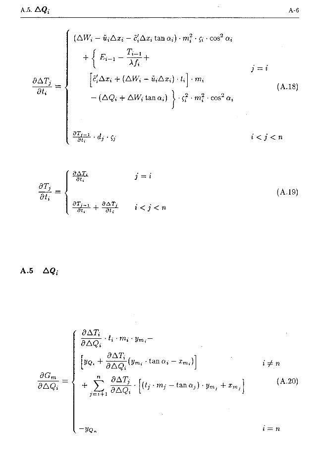
A.5. AQ{ A-6
dATjdtt
(AWt — utAx{ — c'lAxl tan at) • m2 • ft • cos2 al
+ < - ^7T+ J = lc'lAxl -f (AWi — ulAxl) ■ tt ■ mi
(A Qt + A Wi tan ctj) j • (f • m2 • cos2 at(A-18)
dTj-:dt{ ■ d. $3 i < j < n
dTjdt{
' dATi dti
dTj-! 9AT,dti dti
j = *
i < j < n
(A-19)
A.5 A Q{
dGmdA Qi
dA Tio A ^ -ti-mi- ym-O x
dATt ,yQl + a A ^ (ym,- • tan Qi - arm,)
+
dA Qi
^ dA7y dAQi£ (*y • mj - tan aj) ■ ym + x,
i 7^ n
(A.20)
< = /i

A.6. END FORCES A-7
dATtdAQt
(tt ■ ml — tan at) — 1
dGf dA Qi
n
+ Ej=t+i
dA Tj dA Qi
■ (tj • inj — tan aj)i ^ n
(A-21)
-1 i = n
and
d AT3 dAQt
ft j = i
dT,_ dA Qi, * dj ' 0 i < j < n
(A.22)
dTjdAQt
a at,dA Qi
ar,'_! a at,dAQi + dAQi
j = i
i < j < n
(A-23)
A.6 END FORCES
dGmdEa ya + J2
t=l
<9ATt<9£a
(0 • - tan a,) • ymi + xmi
dGf
~dE~a
dATi~dE^
(ti ■ m'i • — tan at)
(A-24)
(A.25)
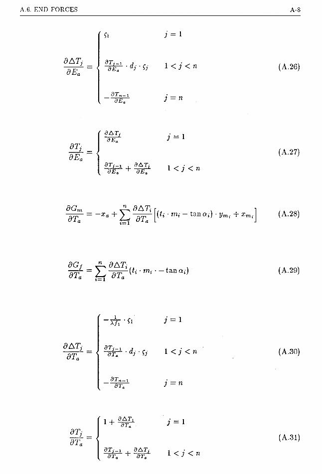
A.6. END FORCES A-8
0 j = 1
dAr,d Ea ^kr ■ dJ • & 1 < i <"
arn_idEa j = n
(A. 26)
a at,dEa
<
dTj_, 9AT,k dEa dEa
j = 1
1 < j < n(A.27)
dTaDATi dTa
(tl ■ wt - tan at) • ym. + xmi (A.28)
dGf~dT\
n OAT,dTa
(ti • mi tan at)
j = 1
dATjdTa
1 < j < n
_dTn-1
, 3Ta j = n
dTjwa
/ 1 + 3 ATX 3Ta<
3T;_! d AT, 3Ta dTa
j = 1
(A.29)
(A.30)
(A .31)1 < j < n

A.6. END FORCES A-9
OGrn
dEb = -Vb (A. 32)
dGf~dE~b
(A.33)
dGmdTb (tn ■ rnn ~ tan an) ■ ymn 4- xmn - xb (A.34)
dGfr.rp — n tan QnoTb
It is worth pointing out that once the values of the parameters are given, the
derivatives can be calculated explicitly and successively using the equations given
in this Appendix. The above formulae are applicable to the case where A is not
zero. If A is zero, which corresponds to the case of simplified Bishop or Janbu
analysis, ATt is identically zero. Therefore, all the derivatives of ATt and Tt are
to be replaced by zero in the above expressions.
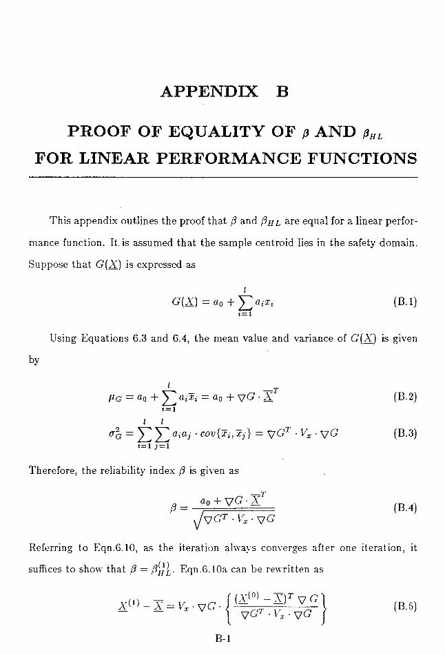
APPENDIX B
PROOF OF EQUALITY OF /? AND aHL
FOR LINEAR PERFORMANCE FUNCTIONS
This appendix outlines the proof that p and Phl are equal for a linear perfor
mance function. It is assumed that the sample centroid lies in the safety domain.
Suppose that G{X) is expressed as
lG(X) =ao + Ya,:r, (B.l)
1=1
Using Equations 6.3 and 6.4, the mean value and variance of G'(X) is given
by
_ jllG — ao + ^ ^ flt^t — ao + yG • A (B.2)
i=i
l i
°~G ~ ai(lj ' cov{*i'*3} = VGT • Vx ■ \/G (B.3)i= i j = i
Therefore, the reliability index p is given as
a0 + VG • X1 \JV GT • Ux • yG'
(B.4)
Referring to Eqn.6.10, as the iteration always converges after one iteration, it
suffices to show that P = Phl,- Eqn.6.10a can be rewritten as
X[l) -X = Vz-yG- (V0) -X)r v G~1VGT ■ \ V ■ vC J
(B.5)
B-l

B. PROOF OF EQUALITY OF P AND fiHL FOR LINEAR PERFORMANCE FUNCTIONSB-2
Note that v^(2Q is constant and independent of the trial value of X_. As the
initial trial point must satisfy the limit state equation G'(X) = 0, therefore
a0 + a‘x\°] = «o + {A0)}r • VC = 0t— 1
=> !I(0)}T-vG=-«o
(B.6)
Consequently,
X*1* -X = Vx- vG-VGr • Vx • VG |
(B.7)
Substituting Eqn.B.7 into Eqn.G.lOb, we obtain
Phl = \ivx'VQT • V<2- (~a0 ~XT V G)(\/Gt ■ Vx •
= |(V<2T • Vx • yG) • (-a0 ~XT V G){\/Gt ■ Vx •
= |(—a0 -XT V G')(vG;r • Vx •
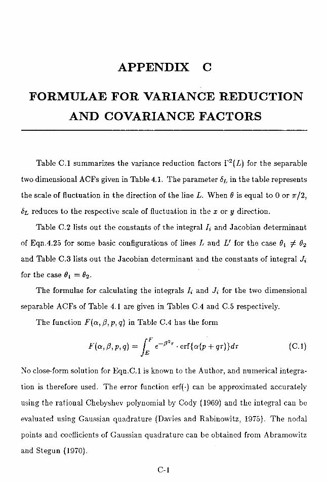
APPENDIX C
FORMULAE FOR VARIANCE REDUCTION
AND COVARIANCE FACTORS
Table C.l summarizes the variance reduction factors T2(L) for the separable
two dimensional ACFs given in Table 4.1. The parameter 8l in the table represents
the scale of fluctuation in the direction of the line L. When 0 is equal to 0 or 7r/2,
8l reduces to the respective scale of fluctuation in the x or y direction.
Table C.2 lists out the constants of the integral It and Jacobian determinant
of Eqn.4.25 for some basic configurations of lines L and V for the case 0\ 7^ Oo
and Table C.3 lists out the Jacobian determinant and the constants of integral Jt
for the case 6X =60.
The formulae for calculating the integrals /t and Jt for the two dimensional
separable ACFs of Table 4.1 are given in Tables C.4 and C.5 respectively.
The function F(a,/3,p,q) in Table C.4 has the form
No close-form solution for Eqn.C.l is known to the Author, and numerical integra
tion is therefore used. The error function erf(-) can be approximated accurately
using the rational Chebyshev polynomial by Cody (1969) and the integral can be
evaluated using Gaussian quadrature (Davies and Rabinowitz, 1975). The nodal
points and coefficients of Gaussian quadrature can be obtained from Abramowitz
and Stegun (1970).
(C.l)
C-l
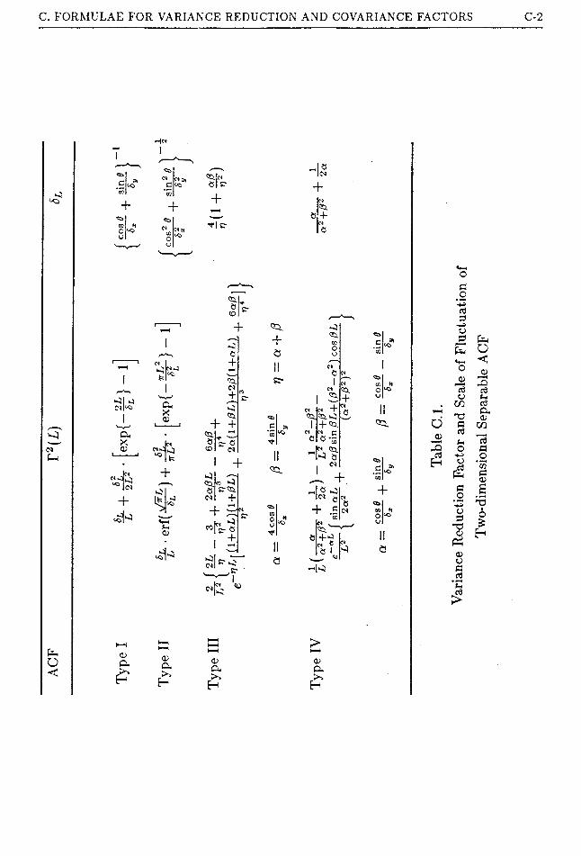
C. FORMULAE FOR VARIANCE REDUCTION AND COVARIANCE FACTORS C-2
fa)c*fa
■-o’+
faXCD
+
+
CV <0
— S'I
faX<u
+
-s’
0>
<^bCl sr
+
T| ST
+
+e
IIOCL
-I®l<N
+
+
«?
«?
<-o*+
«?
oJl)fa
< •—i i—i >fa o »—i W—Ho<
CX>>H
<Dfa>~>
E-
<Dfa>,o>cx>>
H
Var
ianc
e Red
uctio
n Fac
tor a
nd Sc
ale o
f Flu
ctua
tion o
f Tw
o-di
men
sion
al Se
para
ble A
CF

C. FORMULAE FOR VARIANCE REDUCTION AND COVARIANCE FACTORS C-3
Case Configuration Criteria • -4, ct A Ei Fi
61 < 62
1 t’xo ^1 Cl (l’yo — LjSi )CT2
CT2 V XO Vy0CTl CTy Vyo LyS 1 Vy0
L1 Sy < L'2 ■?2 t'xo > LyCy
Vyo ^ LySy
2 vxo LyCy
(vy0 - LySy)CT2
ct2 Vxo Vy0CT2 ct2 Vyo Vyo ~ Li [ S1 + L2S2
3 Vxo + L2C2—
(v y0 + I^S^CTl
CTy Vxo Vy qCT'2 ct2 Vy0 — LySy + L2S2 1 \jO + L2S2
1 Vx0 LyCy
(v,jo — LySy )CT2
ct2 Vxo VygCT 1 Cl 1 Vyo — LySy Vyo -t- LySy + L2S2
61 <C d2
L\S\ > L2S2
Vxo > LXCX
2 t’xo + L2C2 —
(Vyo + LjSoJCTl
CTy Vxo Vy0d T\ CTy Vyo — LySy + A Sn Vyo
Vy0 > LySy
3 t'xo + L2C2 —
(Vyo + LlS^CTy
CTy Vxo Vy0C T2 CT2 Vyo tj’yo + L0S2
1 t’xo ct2 t'xo + L2C2 — LyCy Ty 0 LySy
Oy >62
LySy = L2S2
t'xo Zl L1 Cy2 t'xo -CTy t'xo + L2C2 — LyCy -T2 0 LySy
Vy0 -- 0
n
i| sini — >|
1| sin(0i — S3j|
1| sin(tfi—tf;}|
Table C.2.Jacobian Determinant and Constants of Integral / in Eqn.4.25
for the Basic Configurations of Line Averages [9j 7^ Oo)

C. FORMULAE FOR VARIANCE REDUCTION AND COVARIANCE FACTORS
Case Configuration Criteria
4
61 > S2 L\ S\ >
i'xo > A A Vyo > L2S2
61 > S2 L\S\ < L2S2t'xo ^ L1 C1
Vyo > A So
6
L,S, < L2S2 rJO > A A
I’yo > A Si + L2S2
•At Bi Ct A Ei Ft n
1 t-’xO “f" VyoCT'l -CTi Vxo — A A + -ct2 Vy0 -r L\S\ — L2S2 Vyo -fj L\Sl
[vy0 + AA)CT2
2 l-'xo VyoCTx —CTi vI0 + L2C2+ -CTi Vyo Vyo + A. ~>i — L2S2 i| sin(e1-V2 )|
(ryc) - L2S2)CTi
3 I'xo + VyoCTo -ct2 vT0 4- L2 C2 -f- -CTi Vyo ~ L2S2 JO
(Vyo - L2S2)C7\
1 Vxo -f Vy0CT\ -CTi i’xo ~ L i A -f
{Vyo + L\Sl)CT2—CTo Vyo
2 Vxo "f Vy0CT2 -ct2 Vxo — A A +
(vy0 + AS\)CT2-ct2 Vy0 + L\S i — L2S2
3 Vxo -f Vyo CT2 -ct2 vI0 + L2C2 +(Vyo - L2S2)CTl
-CTi Vyo L2S2
1 Vxo — A C\ -f -CTo Vxo + L2C2 — CTi Vyo — A Si — L2S2
U'yo — L\Si )CT2 (Vyo ~ L2S2)CTl
2 vI0 ~ A A +
(vyo- LiSi)CT2-CTo Vxo + Vy0CT2 -ct2 Vyo L 2*5*2
3 V XO Vy qC'T 1 CTi Vxo "f Vy0CT2 ct2 Vyo L1 5,
t'yo -f A ‘Si
lV‘
tyo -f i — L2S2
Vyo -ft L252
t?yo H A A
Cvo
1| s i n (01 — 0 ;) [
1| sin(6j +»;)|
Table C.2. (cont.)
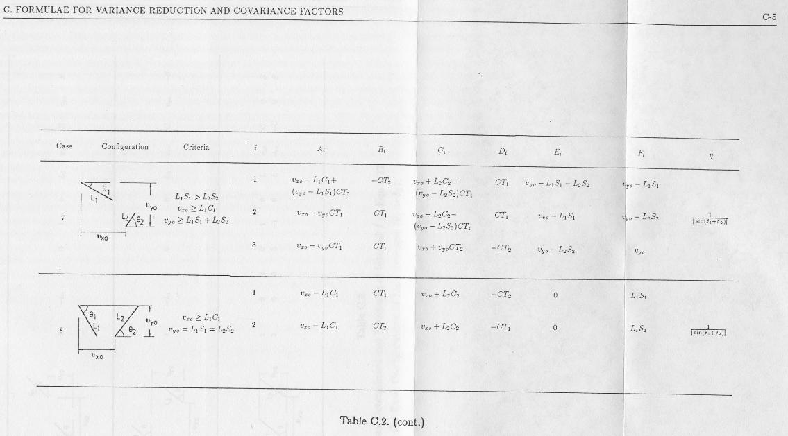
C. FORMULAE FOR VARIANCE REDUCTION AND COVARIANCE FACTORSC-5
Case Configuration Criteria t BC D E* n
*
st t~ -----------r 1 LlCl+ CT- + L2C2 CTx vy0 - LxSx - L2S2 riyo - LxSx' LXSX>L2S2 [Vyo-LxSx)CT2 {Vyo - L2S2)CTx
12/.Q J v >°r~q * r 0 2 vxo - vyoCTx CTX vxo + L2C2- CTX Vyo-LxSx vyo - L.Sn —. 1_______
«Jxo ‘3 vxo - vyoCTx CTX vxo + vyoCT2 —CT2 Vyo — L2S2 vyo
,
1 vxo LXCX CTX vxo + L2C2 —CT2 0
K01 L2/ Uvn vX0>LxCxy^Q2 Vyo = LXSX = L2S2 2 vxo-LxCx CT2 vxo + L2C2 -CTX 0
uxo
LXSX
1 | sintSi+il2)|
----------------------------------------—------------------------------------------- -----
Table C.2. (cont.)

Cas
e
C. FORMULAE FOR VARIANCE REDUCTION AND COVARIANCE FACTORS C-6
al
c*:
o
•X
o
4’
o
Cl
Co co
O o
o oH H3 S
<3 >-3
o ^
Tabl
e C.3
.)b
ian D
eter
min
ant a
nd C
onst
ants
of In
tegr
al I
in Eq
n.4.
27
br th
e Bas
ic C
onfig
urat
ions
of L
ine A
vera
ges (0
\ = 02
)

C. FORMULAE FOR VARIANCE REDUCTION AND COVARIANCE FACTORS C-7
ACF 1 = Ie Ja+Bt[2 p( n. ^)dri dr2
Type I 12 ( p,] (exP{ 2(at + (3tF)} exp{ 2{al + (3tE)}i— i
a,=A Q2=c /J2 = A + g
Type II £ £(_iPi,qi)l— 1
cv = ^ ft — ^ Pi — A P2 — C qi = B q2 = D
Type IIIQ E £(-1)‘+*: exp{-[p. + (9.+ /5)6]}'
i— 1 k— 1f (1 +/?£fc)(2+p, +(], £k) | 0(- + Pi + Qx £k ) + <7i( l + | 2/3(7, 1\ q>+0 1 (<7,+/?)2 1 (<7,+/?)3J
<* = Ji ft~Tv Pi = 01A p2 = aC
ql = aB q2 = oD = E f2 = F
Type IV 2 2 21 y~> y^ y^ / |\t + A: + l exP( "“^7ifc)*[^i sin + cos $ijk\lj -r+"?
« = ^ ft = ^ Pl = ^ P2 — Cqi = B q2 = D = E &> - E
Vik = api + UiZk Vi = otqt + ft Vi = aqt + (3 v2 = aql - (3
$ijk — Vj kk + &Pi ~
Table CU.
Integral I for the Covariance Factor of Line Average (Eqn.4.25)
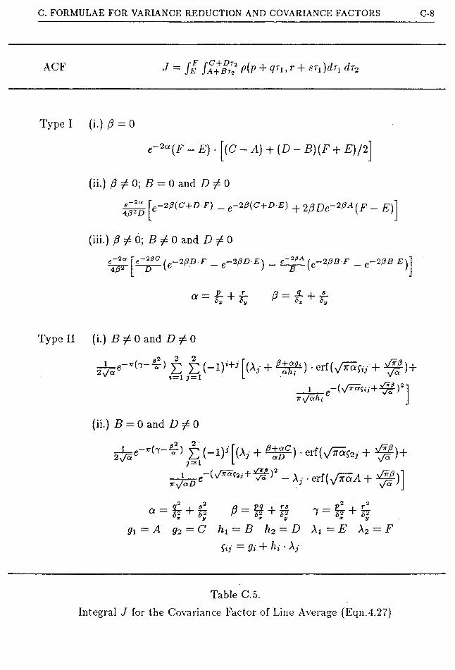
C. FORMULAE FOR VARIANCE REDUCTION AND COVARIANCE FACTORS C-8
ACF J = Je Ia + r’t? PiP + (F\ + )dr{ dr2
Type I (i.) (3 = 0
e~2a(F-E)- (C-A) + (D-B)(F + E)/2
(ii.) /3 ^ 0; B — 0 and D ^ 0
|I^re-2 S(C+DF) _e-20(C+DE) + 2/s De~2l3A (F - E)
(iii.) /? ^ 0; B ^ 0 and D ^ 0
4 /?2,-2 0C (e-2(3D F _ e-2f3D Ej _ e~2/?~4 ^-20B F _ e-2pB Ej
K — JL + JL a ~ 6, +
Type II (i.) B ^ 0 and D ^ 0
2 2Le-»(7-VJ 2 E(-l)<+d(A)- + a±^).erf(Vir«fty + ^)+2 ^/a
i = l J= 1
1 +7Ts/ah,
(ii.) i5 = 0 and D^O
+ £±gC) . + >$■)+
- A, •erf(v/ia/l +3 — 1
i___c-(N/?raf2/+:^f)'7t sfaD
n - al j_ if. - E£ + II - El 4- if.a “ 62 + 62 p - b* ^ bl I — + 61
gx — A g2 = C hi = B ho — D A \ — E A 2 = F$ij — 9i + hi • Ay
Table C.5.
Integral J for the Covariance Factor of Line Average (Eqn.4.27)
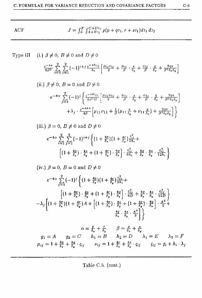
C. FORMULAE FOR VARIANCE REDUCTION AND COVARIANCE FACTORS C-9
ACF J=r /e Ia+Bt? p(p + (Fi T + Su )dn dr2
Type III (i.) (3^0, B ^ 0 and D ^ 0
i= i j — iI /*»£ j_ , f'JJ_ Jl___ I 3 qs
2 ’r /? ‘ ' (3 ' bxV
(ii.) (3 0, B = 0 and
‘-*a
,-APA
S i "2/ 3qrs^2; I'Zj i ^2; _*__,2 0 * by ^ 0 ’ bx ' 0^SX6~
+ AJ ' hf" + + WbTTy
e"4aii.(-i)i+y{< i+^,(i+$)^+(iii.) f3 = 0, B ^ 0 and D/0
2 2E Ii = 1 j = 1
u + £)-£ + (‘ + £)-£
(iv.) f3 = 0, B = 0 and D 0
1 ^ *y
C7 ■ 4 q 4 s <~»>6/i, 6* 5y I2hx
e~4a E(-ip({1 + g)(i + £)^+J = 1
—A
O + fHf + O + fr) 134p 4r
<5y
£y ' 6*4p \ 4s 6 J ‘ 6y
c3.
4r 6y> 6X
4 s *2/ ]*y 12D f
4q~bx
.41 + 2 '
a = t + i
li.ii. a!£y 3
^=*+tg{ — A g-2 — C hi = B h2 — D A \ = E X2 = F
Vij = 1 + If + If * fry *fry - i + fr + I; * fry fry - ft + ^ • h
Table C.5. (cont.)

C. FORMULAE FOR VARIANCE REDUCTION AND COVARIANCE FACTORS C-10
ACF J = Se Ia+Bti P(P + + STijdTi dTo
Type IV (i.) v ^ 0, B ^ 0 and D/0o o
e - ( e.+ i + ir^£ E(-D,+J+Ii = 1 j = 1 hi(7 —1'~) cos(a+7C>y )+2~jiy sin(a + 7f.'> ) . sin(/?+i'f,-y)
(72 + *'2)a ‘ + 2 i/ *
(ii.) v i=- 0, B = 0 and D 0
2 f —ur~‘. r / .2 ,2
5"JS(_1)y+,{1=^ (7* — i/-) cos(g + 7C2j )+27t/ sin(o + 7<~2>) , sin(-?+i,f2;)(7“ -f- i/2 J 2 l o,, 2
+e-vD 7 sin (a+ 7/? ) — i' cosfa-f vB ) , sin(/3-fi'£?) — cos( f3+i.'B ) (72 + t/2) 21'
2i'~
(iii.) i/ = 0, B ^ 0 and D ^ 0
tEE(-')’w -cosfg1=1J=1 L
2 2 cos(a+7f,y) C,
(iv.) i/ = 0, Z? = 0 and D yt 0
!r||(-i))>1{c”y - cos/? ■ § + p-y+^? - cos/3 ■ y|] ■ |
a — JL _ JL /? — + JL ^ — JL _ JL -y = JL + 2La - 6, 5V P ~ Sx ^ 7 5, ^ ty
gi = A g2 — C hi — B ho — D A \ — E \o — F
$ij — 9i d~ hi * Ay
Table C.5. (cont.)

APPENDIX D
SAMPLING VARIANCE OF VARIANCE PLOT
This appendix shows the calculation of variance of in Section 5.2.3.2. With
out loss of generality, it is assumed that E{Kt} = 0. It is also assumed that
follows a joint Gaussian distribution. The soil property at t — (see Fig.5.1) is
denoted simply as Kt and p(tt) by p(i). We have
Nn
N,
Nr
D*"1 = 1
Nn
i = li Nn n
Ki+j-1 - Nn n E E *+>■n " 7~r 77Ti=ij=lN n n n
N„n2 EEE^-1n i=i j = i j'=i
i iVn ATn n n
S S ’ **'+>'-1Ar2;l2.................n i= 1 i' = 1 j — 1 j ' = 1
(D.l)
By definition
rar{s“} = £{(s“)2} - |E{s“}|“ (D.2)
The second term on the right hand side of Eqn.D.2 can be obtained using Equations
D-l

D. SAMPLING VARIANCE OF VARIANCE PLOT D-2
5.47 and 5.48. Therefore, it suffices to discuss the first term in the equation.
£{(4)2}Nn n n
1
Ki+j— 1 Ki+j' — 1
Nn Nn n nELEE Ki+y-,K,■<+;<-1\ ro o—,i=i t'=i j = i j'= i
ATn Nn n n n n_£{ A'2n4 J2YU212J2Y, Ki+j-lKi+j'-lKi'+p-lKi'+p'-ln 1= 1 j' = 1 J = 1 j' = 1 p= 1 p' = 1
cy N n N n Nn Tl Tl Tl Tl
~ JpZA zL ]C Ki+J-l^+j'-l^ + g-lKy + g'-ln i= 1 p= 1 p' = 1 _/ = 1 j ' = 1 g= 1 q'= 1
1 Nn Nn Nn Nn n n n n
+ A'l„4 V + , <-ln t—1 t' —1 p=l p'=l J = 1 j'=l gr=l “1
(D.3)
Denote the first, second and third term of the last expression by Ai, A2 and
A3 respectively. Here, a standard result is used for jointly standardized Gaussian
variates Xt (Isserlis, 1915&1918).
£{-Y, A2.Y3.vn = £T{.Y,A2} • E{AVY,} + E{.V,.Y,} • £{.Y2.Y4}
+ E{A’, A’-i} ■ E{ A'o A'3}(D,l)
Using the above result, the following expressions for Ai, An and A3 can be ob
tained.
^1 A
Arn Nn n n n n
p(\i - i' + j- p|) • p(\i - i' + j' - p'\) +
p(\i - % +j - p'\) • p(\i - i' + j' - ;;|)|
P(\j ~ j'\) ■ P(\P~P'\) +

D. SAMPLING VARIANCE OF VARIANCE PLOT D-3
a n4
4 n —1
- M) ■ p(r)
r4 Nn-1
2p(\i - i' + j - p|) • p(\i -i* + j ~p
2[ E i“Lr = ^-l)
O^j-4 A rV2-? 0v„-|rl) ]T («- |s|) •P(lr + «l) (D.5)i r=-(AC,-l) Ls = -(n-l) J
Similarly
A^> — y y y (Nn -M)(n-M)(n-i(i)-/j(s) •/>(»•+o' r=-(N^-l) s = —(n —1) t = -(n —1)
4(7 4 Nn _Nn n n
+ wDLEE'l|i+J-p-,l)t = 1 P=1 J = 1 <7— 1
(D.6)
A** — iVirc4 (An - M)(»- M) -p(V + *1)Lr= — (Nn — 1) s = —(n —1)
+9 4 A'n Nn n n
wEEEE'i"n n Li=l p = l j = l g=l+y-p-?i) (D.7)

APPENDIX E
TECHNIQUES OF
RATIONAL APPROXIMATION
The Technique of rational Approximation has wide applications in engineer
ing analysis which are discussed in some detail in Li and White (1987d). This
Appendix only outlines the relevant techniques which have been used in solving
some of the problems in this work.
E.l SOLVING NON-LINEAR EQUATIONS
Given a non-linear function g(x). The problem arises of solving the equation
g{*) = o (E.i)
It is assumed that the equation has a single root at x = a. In engineering analysis,
it is common that g(x) is only expressed implicitly in terms of x or that the function
is so complicated that it does not lend itself to solution using techniques which
require the knowledge of the derivatives such as the Newton-Raphson's method.
Initially, the values gt = g(xt). i — l.m. are calculated for in different values
of x. The inverse function of g{x), designated as i](g), can be approximated by
the following rational polynomial expressed in the form of a continued fraction.
E-l

E.l. SOLVING NON-LINEAR EQUATIONS E-2
x - T](g) & ai 4-
d 2 +
g- gi
g-g2(E-2)
a 3 +. g gm—i
’ • H--------------dm
The coefficient at in Eqn.E.2 can be computed using the procedure described in
Table E.l.
d\ dn d3 a4
d\ = XX
d'2 1 — Xo a — Jfc--------Q±_doX - ax
d3l = X3 n — 17.3 - 1713- a3l - ax
_ 173 - g-23 a32 ~ a2
a41 ~ X\ n — 174 — g\4“ a41 -
- _ 174 ~ 172043 a42 - «2
„ _ 174 — 17.34 a43 - a3
Table E.l Coefficients of Rational Polynomial
Since a = r;(0), an approximate solution of the root can be obtained by
substituting g — 0 into Eqn.E.2 giving
9ict ~ -r m + i — ai
a o —172
(E.3)
gm-ldm
d 3 -

E.2. OPTIMIZATION E-3
The value of g(x) corresponding to the approximate solution xm+i is then
computed. With this new data point, a better approximation to T](g) can be
obtained by lengthening the continued fraction to (m + 1) terms. The above
procedure is then repeated until the required tolerance for g(x) is achieved. It
should be noted that the addition of an extra data point to the continued fraction
does not require any re-ordering of the continued fraction or re-calculation of
the previous coefficients. Only the coefficient am+l needs to be evaluated. The
iteration procedure of Eqn.E.3 has an order close to 2 (Li and White, 1987d) and
hence it has efficiency comparable to Newton-Raphson’s method.
E.2 OPTIMIZATION
E.2.1 Univariate function
Only the case of minimization will be considered here. The procedure for
maximization of functions is entirely similar.
E.2.1.1 Theory
Given a unimodal function g(x) with a unique minimum value gp at the point
xp. The basic approach for searching for the position of xp may be divided into
two steps:
(1) locating the interval within which the optimum position xp lies;
(2) searching for the optimum position within the interval.
The first step can be done using the forward-backward method. Suppose that
Xo is the initial estimate of the optimum point xp and h (h is positive) is the initial
step size. It is required to find an interval [ xi,xu ] such that xp E [ xi,xu ]. The
procedure is as follows:
Forward calculation:- Firstly, the value of g(x0) and g(x0 -f h) are computed. If
(7(2:0) > y(-To T-/i), the optimum position should be on the right of x0. The step size

E.2. OPTIMIZATION E-4
is then doubled and the value g(x0 +3h) is calculated. If g(x0 +h) < g(x0 +3/i), it
is obvious that xp is bounded by Xq and Xq +3h. The interval [ x*, xu ] is therefore
[ 2r0, xQ +3h ]. If <7(2:0) > g(x0 +3/i), the search continues in the forward direction,
doubling the step size of each iteration.
Backward calculation:- If <7(2:0) < g(x0 + /i), the value of <7(2:0 — h) is evaluated.
If g(x0 — h) > <7(2:0), the required interval becomes [x0 — h, x0 + h }. Otherwise,
the current step size is doubled and the search continues in the backward direction
until the interval is identified.
The procedure of the forward-backward method is summarized in the flow
chart of Fig.E.l.
initialise x0, hXC - Xqxu = xc + h xi — xc ~ hwhile g[xu) < g(xc) do
h = 2 hXL = Xc
xc — xuXu — xu -{- h
endwwhile g(xt) < g(xc) do
h = 2hXu — X c
X c X[
xi — X[ — hendw
Figure E.lComputer Pseudo-code for Forward-backward Method
(after Li and W hite, 1987c!)
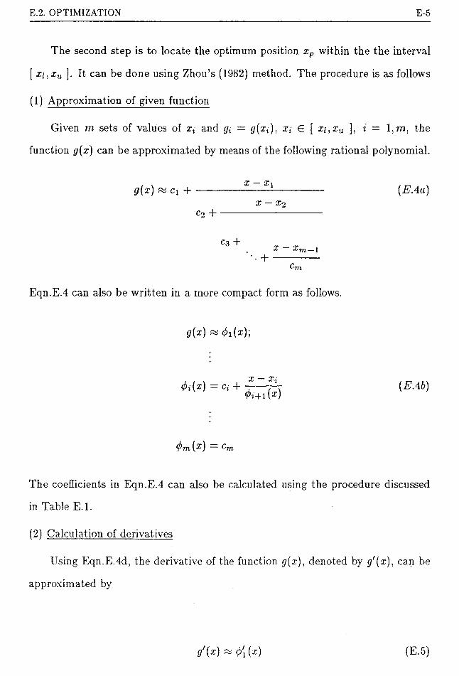
E.2. OPTIMIZATION E-5
The second step is to locate the optimum position xp within the the interval
[ xi, xu ]. It can be done using Zhou’s (1982) method. The procedure is as follows
(1) Approximation of given function
Given m sets of values of xt and gt = g{xi), xx E [ xi,xu ], i = 1 , m, the
function g(x) can be approximated by means of the following rational polynomial.
/ X , X- Xig(x) « ci +-----------------------------X — X‘2
Co H---------------------------
C3 + X ~ XJn_l•• + ------------
Cm
Eqn.E.4 can also be written in a more compact form as follows.
(EAa)
g(x) & 0!(x);
</>i(x) = ct +X - Xj
(EAb)
&771 (*C) — C7n
The coefficients in Eqn.E.4 can also be calculated using the procedure discussed
in Table E. 1.
(2) Calculation of derivatives
Using Eqn.E.4d, the derivative of the function g(x), denoted by g'(x), can be
approximated by
ff'(x) PS # (x) (E.5)

E.2. OPTIMIZATION E-6
The derivatives of g(x) at the trial points xt, i — 0, m are given by
g[ = g'(xt) & <t>\(xi)
) ~ (art - xi) • [03(*i)]2
&] + 1 (^t) (•£» j'-(. i (*^t)[0j + l(*t)l2
j < i
( 0$(*») = < 1
if i — m;
otherwise.(E.6)
(3) Approximation of derivative function
As the function gf(ar) is assumed to be unimodal, <7'(a;) is therefore a monotonic
function and hence an inverse function for it exists. Given the m initial trial values
of xt and with the corresponding values of g[ calculated using Eqn.E.6, the inverse
function of g'(x), designated as w(g'), can be approximated by another rational
polynomial:
x = w(g') di + g' - g\
do +g' - g-2
(E.7)
do, T / /g - gm-1
*• + ------ :--------
Again the coefficients in Eqn.E.7 can be computed using a procedure similar to
that described in Table E.l.
(4) Iteration for solution
Since the optimum point xp is given by the solution of the equation g'(:r) = 0,
an approximate solution for xp can be obtained by substituting g' — 0 into Eqn.E.7.

E.2. OPTIMIZATION E-7
Thus
Xp K, Xm -)_ i (E.8)
(h — g'm-1
d m
The corresponding value of <7m+1 is then evaluated. With these new values of
xm + i and gm +1, it is possible to obtain a better approximation to the function
by lengthening the continued fraction of Eqn.E.4 to ra + 1 terms. The procedure is
then repeated using Equations E.6, E.7 and E.8 until the change of x for successive
iterations is small or the value of g'(x) is sufficiently close to zero.
Four is usually a good starting value for the number m. The current value
of xi, xc and xu obtained from the first step (see Fig.E. 1) can be used as the
first three trial values xt, i — 1,3. The fourth trial value can be obtained using
the quadratic interpolation technique. Since the values of the function g(x) at
xi,xc and xu have already been calculated, a quadratic response curve may be
fitted through these three points. The location of the optimum point xp can be
estimated by the minimum point of the response curve, denoted by z4, and it is
given by
1 (xl - xpgx + (.rg - x\)g2 + (j? - x%)g32 (Xo - x3)gi + (x3 - xi)go + (xx - x2)g3
(E.9)
Since gc is always less than gi and gu, x4 must lie between xi and xu and
therefore it must be bounded by the interval [ xi,xu ]. These four trial values can
be input into Eqn.E.4 to iterate for the minimum point.

E.2. OPTIMIZATION E-8
H * 4m-0.25
Figure E.2Geometry of Vertical Cut Slope for Example E.l
E.2.1.2 Illustrative Example
Example E.l The factor of safety with respect to height for a vertical cut slope
with straight-line failure surface is given as (Fig.E.2) (Jumikis, 1962)
F =2c't/72c't77
i
cos 9 (sin 9 — cos 9 • tan (})') x2 + H2
xH — x2 tan(E.10)
where c' is the effective cohesion, the effective angle of internal resistance and 7
the unit weight of the soil. Find the minimum factor of safety given that 0' = 30°
and c’ftH — 0.25.
Solution: Table E.2 show the calculations for finding the optimum location and
the minimum value of the factor of safety. Two methods were used, namely, the
method of quadratic interpolation and Zhou’s method. The method of quadratic
interpolation is discussed in Beveridge and Schehter (1970). Although in practice
it is meaningless to evaluate the factor of safety to such a high accuracy, it is for
the sake of illustrating the efficiency of Zhou’s method. It can be seen from Table
E.2 that the convergence for Zhou’s method is extremely fast. Only eight data
E.2. OPTIMIZATION E-9
points are enough to achieve a tolerance of less than 10~9. If the method of ‘golden
section' (see Beveridge and Schehter, 1970) were used, at least 45 steps would have
been required to achieve the same accuracy. The method has also been applied
successfully to searching for the critical slip surfaces in slip stability problems (Li
and White, 1987a).
E.2.2 Multivariate functions
Numerous numerical techniques for optimizing multivariate functions are avail
able in the literature. Only two methods which have been used in the present study
will be mentioned here. The first method is the technique of alternating variables
and the other is the method of steepest descent. These two methods are discussed
in many books on optimization such as Beveridge and Schehter (1970) and Jacoby
et a/ (1972) to which readers may refer for details.
E.2.2.1 Technique of alternating \~ariables
The use of the technique of alternating variables involves the following steps.
Given a n-dimensional function H(X) and an initial estimate of the optimal point.
Each variable is chosen in turn and all the other n — 1 variables are held constant.
The optimal point with respect to the chosen variable is obtained. The variable is
then fixed at this ‘conditioned’ optimum point and the procedure is repeated for
the next variable. Once all the variables have been searched, the process will be
started again from the first variable. The procedure is repeated sequentially until
the required accuracy is achieved.
The procedure is best illustrated by means of a two-dimensional function as
shown in Fig.E3. Starting at the initial point A, the function is searched along
the AVaxis until the ‘conditioned’ optimum point is reached at point B. Keeping
the value of X\ at this optimum value, the function is then searched along the
Xo direction until again it reaches the second ‘conditioned’ optimum point C. By
repeating the above process, the search will gradually advance towards the global
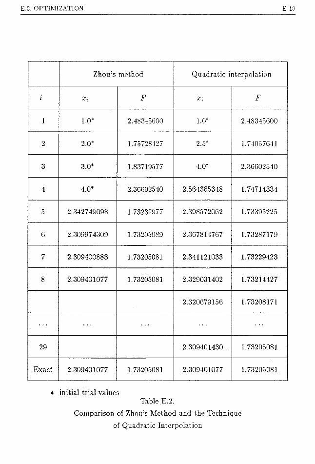
E.2. OPTIMIZATION E-10
Zhou’s method Quadratic interpolation
i •O F F
1 1.0* 2.48345600 1.0* 2.48345600
2 2.0* 1.75728427 2.5* 1.74057641
3 3.0* 1.83719577 4.0* 2.36602540
4 4.0* 2.36602540 2.564365348 1.74714334
5 2.342749098 1.73231977 2.398572062 1.73395225
6 2.309974309 1.73205089 2.367814767 1.73287179
7 2.309400883 1.73205081 2.341121033 1.73229423
8 2.309401077 1.73205081 2.329031402 1.73214427
2.320679156 1.73208171
29 2.309401430 1.73205081
Exact 2.309401077 1.73205081 2.309401077 1.73205081
* initial trial valuesTable E.2.
Comparison of Zhou’s Method and the Technique
of Quadratic Interpolation
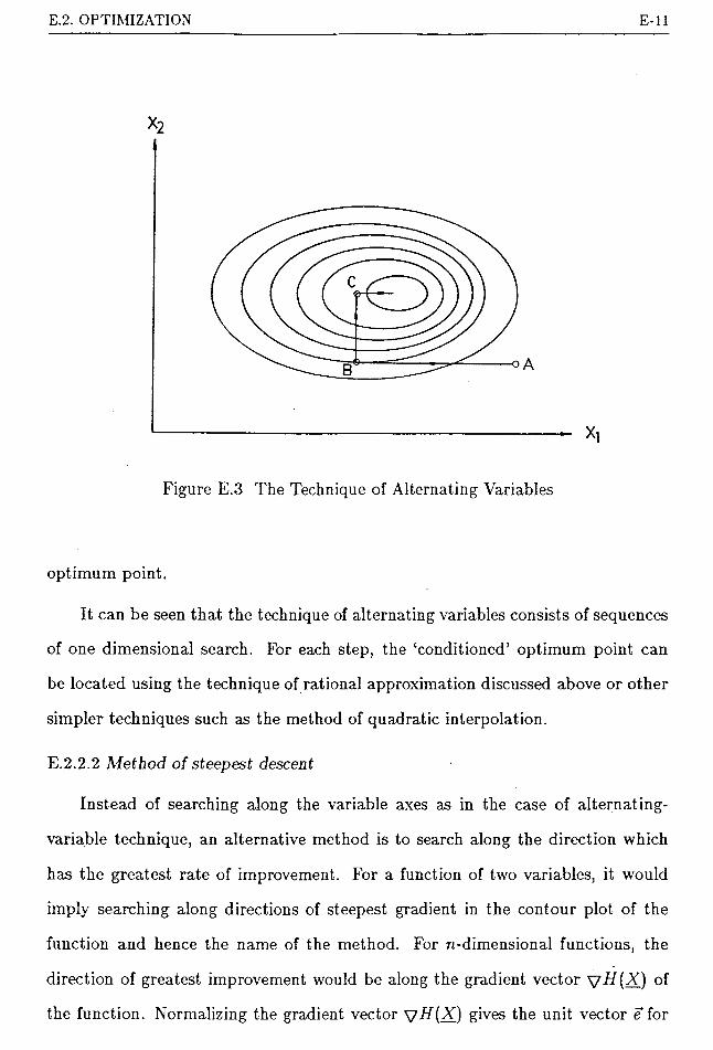
E.2. OPTIMIZATION E-ll
X2
Xl
Figure E.3 The Technique of Alternating Variables
optimum point.
It can be seen that the technique of alternating variables consists of sequences
of one dimensional search. For each step, the ‘conditioned’ optimum point can
be located using the technique of rational approximation discussed above or other
simpler techniques such as the method of quadratic interpolation.
E.2.2.2 Method of steepest descent
Instead of searching along the variable axes as in the case of alternating-
variable technique, an alternative method is to search along the direction which
has the greatest rate of improvement. For a function of two variables, it would
imply searching along directions of steepest gradient in the contour plot of the
function and hence the name of the method. For n-dimensional functions, the
direction of greatest improvement would be along the gradient vector VH(X) of
the function. Normalizing the gradient vector syH(X) gives the unit vector e for

E.2. OPTIMIZATION E-12
the direction of search, viz,
V //(V)I V H(X)I
(Ell)
where
VH(X) =dll dll dHdXi ’ dX-2 ’ " ‘ ’ dXn
dH\212
x2
Figure E.4 Method of Steepest Descent

E.2. OPTIMIZATION E-13
Fig.E4 illustrates the method of steepest descent for a function of two vari
ables. The unit vector ex for the first descent is calculated at the initial point A.
The search is then started along this direction until it reaches the ‘conditioned’
optimum point B. The unit vector e2 of the steepest descent at B is then evaluated
and the search then proceeds along this direction. The procedure is then repeated
until the stopping criterion is satisfied. For explicit functions, the derivatives may
be calculated analytically as in the case of finding the lower and upper bounds of
the performance function in Section 6.4.1. For implicit functions, finite difference
approximation can be used.
For each descent, the locus of the movement X is described by
X — Xi + A • el+1 (E. 12)
where Xi is the location after the z’th descent, el+x is the unit vector of steepest
descent for the (i *f 1) search and A is a location parameter. The parameter
A is searched until a ‘conditioned’ minimum value along the direction el+i is
reached. The resultant location will then form the starting point for the next
search. Therefore, the method of steepest descent can be treated as a series of
one-dimensional search with the objective function treated as a one-dimensional
function of A for each step. Again to find the optimum value of A, the technique
of rational approximation or the method of quadratic interpolation can be used.

APPENDIX F
SOIL DATA
DATA SET 1
The first set of data is extracted from a cone resistance record obtained from a
cone penetrometer test carried out on the southern slope of Mount Cullarin, south
of Goulburn, New South Wales. The data correspond to measurements taken
between a depth of 3m to 4.5m. The soil is mainly a silty clay. No significant
trend is observed for this section of the profile and it can therefore be modelled
as a Type I profile. The measurements are taken at equal intervals of 0.02m and
the total number of data points is 76. The data are listed in Table F.l and also
plotted in Fig.F.l.
DATA SET 2
The second set of data is modified from Table 28 of Agterberg (1974), which
gives the sample ACF of the logarithmically transformed zinc values. The sample
ACF shows a distinct nugget effect which is common for mineral ore. The nugget
effect has been removed and the resulting sample ACF values are listed in Table
F.2. The sampling interval of the zinc values is 0.2m.
DATA SET 3
The third set of data is read from Fig.6 of Yanmarcke (1977c). This corre
sponds to the variance plot of initial void ratio of a soil. The values read from the
figure are given in Table F.3. The sampling interval is 5ft.
F-l

F. SOIL DATA F-2
1.0 30__ i
Qc (MPa)
Figure F.l Cone Resistance - Soil Data Set 1

F. SOIL DATA F-3
Depth Qc Depth Qc Depth Qc
3.00 2.26 3.52 1.70 4.04 2.483.02 2.33 3.54 1.05 4.06 2.283.04 2.41 3.56 1.26 4.08 2.053.06 2.50 3.58 2.05 4.10 2.023.08 2.39 3.60 1.93 4.12 1.983.10 2.50 3.62 1.81 4.14 1.983.12 2.21 3.64 1.77 4.16 1.933.14 2.40 3.66 1.71 4.18 1.943.16 2.02 . 3.68 1.69 4.20 1.923.18 1.88 3.70 1.63 4.22 1.893.20 1.83 3.72 1.60 4.24 1.963.22 1.91 3.74 1.60 4.26 1.993.24 2.28 3.76 1.53 4.28 1.983.26 2.19 3.78 1.46 4.30 1.973.28 2.68 3.80 1.40 4.32 1.993.30 2.62 3.82 1.42 4.34 1.953.32 2.45 3.84 1.39 4.36 1.843.34 2.25 3.86 1.44 4.38 1.843.36 2.34 3.88 1.55 4.40 1.843.38 2.61 3.90 1.55 4.42 1.853.40 2.89 3.92 1.46 4.44 1.863.42 2.84 3.94 1.39 4.46 1.893.44 2.26 3.96 1.58 4.48 1.923.46 2.14 3.98 1.81 4.50 1.913.48 1.91 4.00 1.703.50 1.72 4.02 1.81
Table F.l. Cone Resistance (qc) in MPa - Data Set 1.

F. SOIL DATA F-4
h P(h) In p(h)
1 0.916 -0.087
2 0.508 -0.677
3 0.465 -0.766
4 0.345 -1.064
5 0.447 -0.805
6 0.349 -1.052
7 0.173 -1.754
8 0.254 -1.370
9 0.179 -1.720
Table F.2. Modified Sample ACT of Zinc Values.
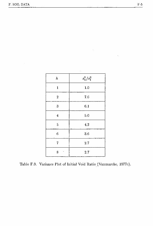
F. SOIL DATA F-5
h 0/0
»n/« T
1 1.0
2 7.6
3 6.1
4 5.0
5 4.2
6 3.6
7 2.7
8 2.7
Table F.3. Variance Plot of Initial Void Ratio (Vanmarcke, 1977c).