Investigation to slope instability along railway cut

Investigation to slope instability along railway cutslopes in Eastern Ghats mountain range, India:A comparative study based on slope mass rating,Bnite element modelling and probabilistic methods

AMULYA RATNA ROUL1, SARADA PRASAD PRADHAN

1,* and DURGA PRASANNA MOHANTY2

1Department of Earth Sciences, Indian Institute of Technology Roorkee, Roorkee, India.

2Department of Geology, Savitribai Phule Pune University, Pune, India.*Corresponding author. e-mail: [email protected]

MS received 17 January 2021; revised 2 June 2021; accepted 8 June 2021

In slope stability analysis, identiBcation of the mechanism behind slope failure is the key factor during thestudy. Rock mass characterization and kinematics analysis, like geotechnical investigation methods, arenot infallible all the time for the weathered slopes. The presence of different grades of weathered mass onthe slope proBle acts independently to inCuence the overall failure pattern. Numerical analysis by Bniteelement method (FEM) is evolved as a primary slope stability analysis tool by overcoming the limitationsof the stratiBed weathered materials on the slope. The paper focuses on the stability analysis of railway-cut laterite slopes of the Eastern Ghats of India. The medium to high-grade metamorphism, followed byphysio-chemical weathering, favours the region for more prone to failure. The Force Equilibrium Modeland Moment Equilibrium Model have been considered to determine the possibility of independent failureevents for the probability analysis. Monte Carlo’s probability simulation method has delivered a betterresult for the weathered slopes by taking many variables for the studied region. A compression study hasbeen made between the outcomes of slope stability analysis methods and the probability analysis models,which provides a comprehensive list of factors to understand the failure mechanism of weathered slopes.

Keywords. Slope stability analysis; rock mass rating; slope mass rating; numerical analysis; railway-cutslopes; laterite proBle.

1. Introduction

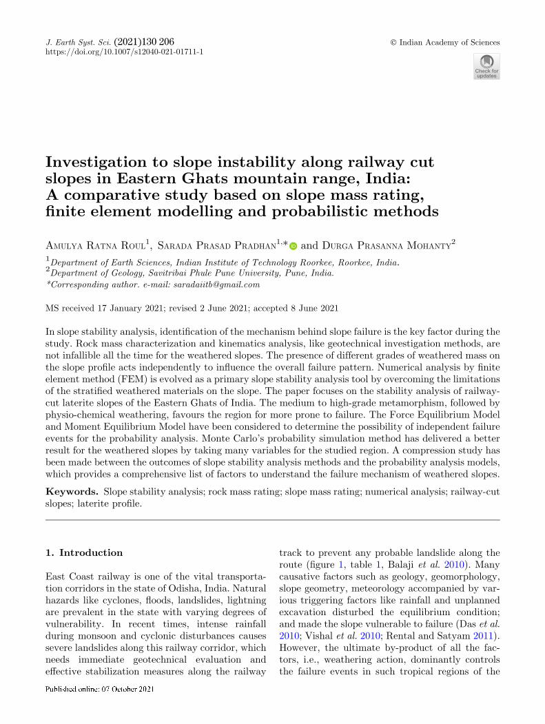
East Coast railway is one of the vital transporta-tion corridors in the state of Odisha, India. Naturalhazards like cyclones, Coods, landslides, lightningare prevalent in the state with varying degrees ofvulnerability. In recent times, intense rainfallduring monsoon and cyclonic disturbances causessevere landslides along this railway corridor, whichneeds immediate geotechnical evaluation andeAective stabilization measures along the railway

track to prevent any probable landslide along theroute (Bgure 1, table 1, Balaji et al. 2010). Manycausative factors such as geology, geomorphology,slope geometry, meteorology accompanied by var-ious triggering factors like rainfall and unplannedexcavation disturbed the equilibrium condition;and made the slope vulnerable to failure (Das et al.2010; Vishal et al. 2010; Rental and Satyam 2011).However, the ultimate by-product of all the fac-tors, i.e., weathering action, dominantly controlsthe failure events in such tropical regions of the

J. Earth Syst. Sci. (2021) 130:206 � Indian Academy of Scienceshttps://doi.org/10.1007/s12040-021-01711-1 (0123456789().,-volV)(0123456789().,-volV)

world. The good drainage pattern of the EasternGhats region with the tropical climate favours thelaterization process to occur on the highlydeformed metamorphic rocks of Eastern Ghatsformation. Depending upon the portion exposed tolaterization, the degree of weathering varies fromthe top to bottom of the mountain sections, whichcauses a challenging task for the researchers totreat the whole section as a single slope in stabilityanalysis. Therefore, a detailed Beld investigationwas carried out to identify the different weatheredzones on a slope. This will substantiate theunderstanding of the mechanism of possible slopefailure. In a general scenario, the failure events aremostly occurred after and during the precipitationin the Eastern Ghats (table 1). It is supposed to bedue to the reduction of the shear strength material

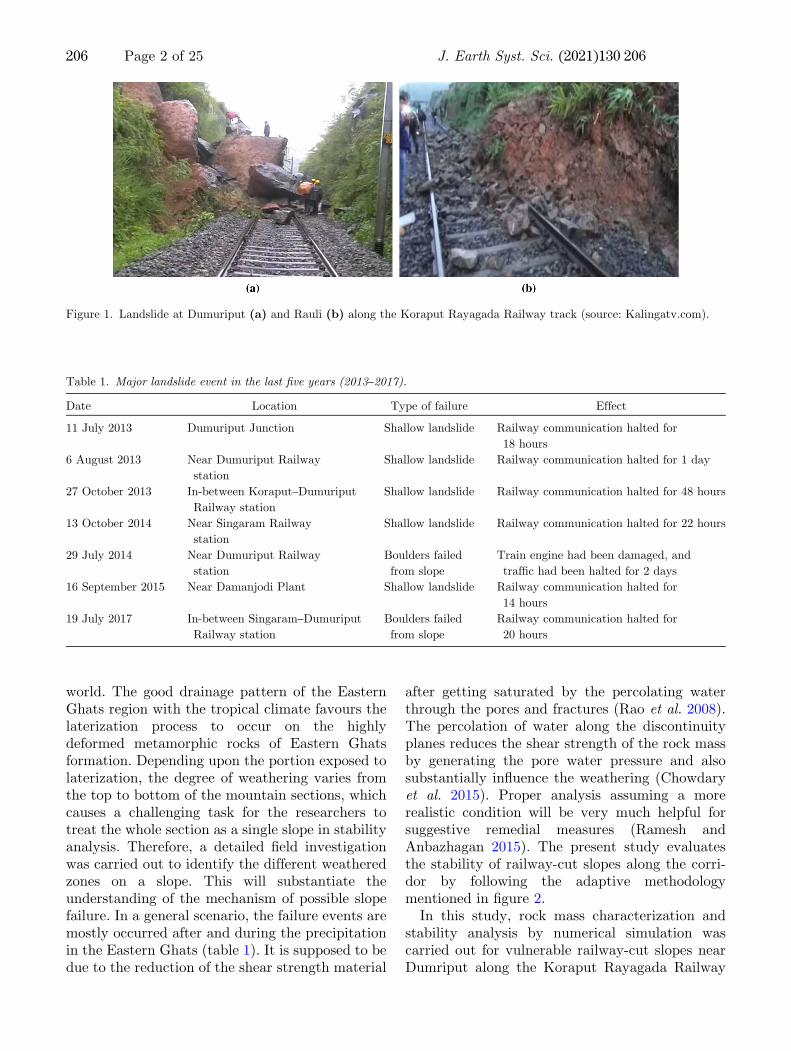
after getting saturated by the percolating waterthrough the pores and fractures (Rao et al. 2008).The percolation of water along the discontinuityplanes reduces the shear strength of the rock massby generating the pore water pressure and alsosubstantially inCuence the weathering (Chowdaryet al. 2015). Proper analysis assuming a morerealistic condition will be very much helpful forsuggestive remedial measures (Ramesh andAnbazhagan 2015). The present study evaluatesthe stability of railway-cut slopes along the corri-dor by following the adaptive methodologymentioned in Bgure 2.In this study, rock mass characterization and

stability analysis by numerical simulation wascarried out for vulnerable railway-cut slopes nearDumriput along the Koraput Rayagada Railway

Figure 1. Landslide at Dumuriput (a) and Rauli (b) along the Koraput Rayagada Railway track (source: Kalingatv.com).

Table 1. Major landslide event in the last Bve years (2013–2017).

Date Location Type of failure Effect

11 July 2013 Dumuriput Junction Shallow landslide Railway communication halted for

18 hours

6 August 2013 Near Dumuriput Railway

station

Shallow landslide Railway communication halted for 1 day

27 October 2013 In-between Koraput–Dumuriput

Railway station

Shallow landslide Railway communication halted for 48 hours

13 October 2014 Near Singaram Railway

station

Shallow landslide Railway communication halted for 22 hours

29 July 2014 Near Dumuriput Railway

station

Boulders failed

from slope

Train engine had been damaged, and

trafBc had been halted for 2 days

16 September 2015 Near Damanjodi Plant Shallow landslide Railway communication halted for

14 hours

19 July 2017 In-between Singaram–Dumuriput

Railway station

Boulders failed

from slope

Railway communication halted for

20 hours

206 of 25 J. Earth Syst. Sci. (2021) 130:206

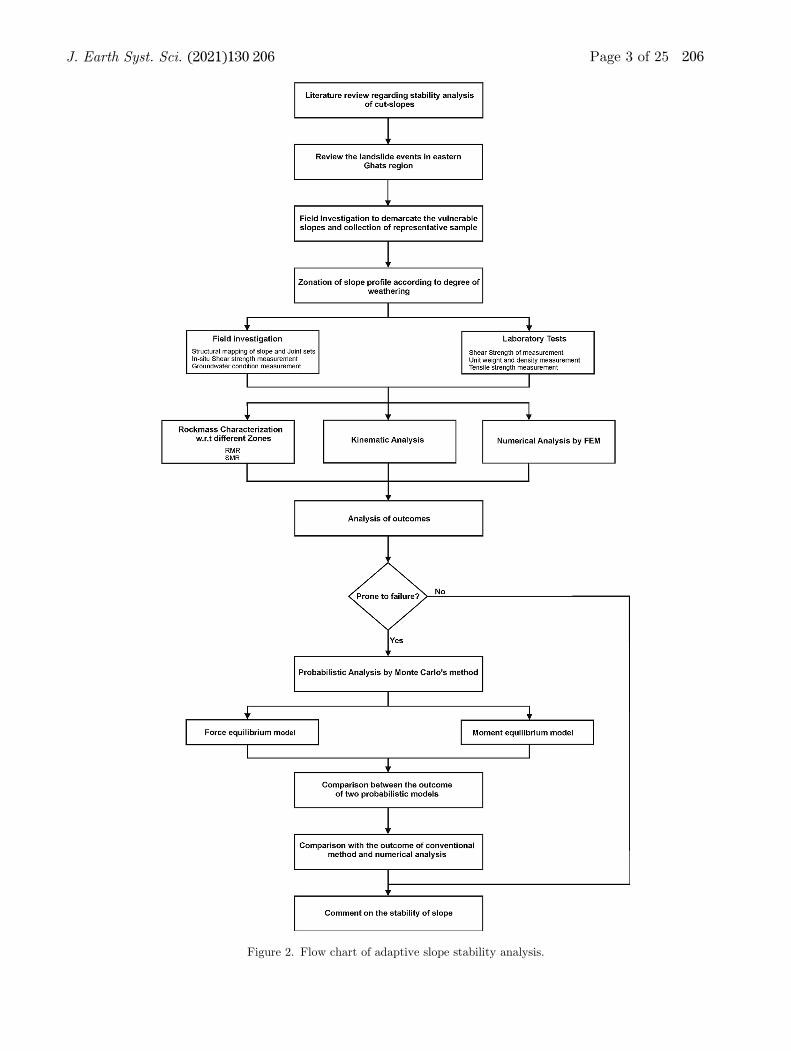
Figure 2. Flow chart of adaptive slope stability analysis.

J. Earth Syst. Sci. (2021) 130:206 of 25 206

track (Bgure 3). Slope instability depends on theslope’s geometry, strength parameter of the slopematerials, geo-hydrological conditions, and struc-tural characteristics of the discontinuities. Rockmass rating (RMR) is a quantitative rock massclassiBcation method, which is an algebraic sum ofthe rating value of six parameters of the rock mass.According to each evaluated parameter, a ratingvalue is assigned to it. But this method cannot givea quantitative description for the orientation ofdiscontinuities on rock mass. So to overcome thisissue, Romana proposed slope mass rating (SMR)in 1985. It gives an edge over RMR for stabilityanalysis (Pradhan et al. 2011). Nowadays, numer-ical simulation is widely used for stability analysisas it is a robust analysis method (Matsui and Can1992; Eberhardt et al. 2004; Vishal et al. 2010;GrifBths 2015; Pradhan et al. 2015; Singh et al.2015; Vishal et al. 2015). The conventional method,like the limit equilibrium method, is a very

simpliBed analytical tool for slope stability analy-sis. Still, Bishop’s method (Bisop 1955), Janbu’smethod (Janbu 1954), and Spencer’s method(Spencer 1967) have some assumptions for theprocessing of data. Later, to overcome the limita-tion issues, the Finite Element Method (FEM),Boundary Element Method (BEM), and FiniteDifference Method (FDM) are proposed and alsobecame very popular for their simpliBed process. Inthe present article, the FEM-based model waschosen over the limit equilibrium method (LEM)due to its advantages like: (a) it generates thecritical failure surface automatically by computingthe gravity loads and the reduction of shearstrength, (b) there is no need of assumption of thedistribution of interslice shear force, and (c) it isable to compute very complex conditions and givequantitative information of stresses, movementsand pore pressures (GrifBths and Lane 1999; Chenget al. 2007).

Figure 3. Koraput–Rayagada railway track along the Eastern Ghats.


In many instances, where rock mass characteri-zation is performed, the whole exposed slope massis taken as a single rock mass irrespective of thedifferent geotechnical characters. To assign a singleRMR or SMR value to the entire rock mass is notan appropriate procedure in slope stability analy-sis. Similarly, numerical modelling considers thewhole weathered rock-mass slope as a homogenousmaterial may have added error to the stabilityanalysis. This is because of the variation in theweathering grade of rock mass from top to bottomof a slope which results in the difference ingeotechnical characteristics for rock mass at adifferent height.Uncertainty and variability in properties of geo-

material are unavoidable in slope stability studiesdealing with weathered materials. However, prob-abilistic analysis is an operational tool to quantifythe model’s uncertainty and variability. Particu-larly for rock slopes, the change and variability inrock mass parameters have been addressed duringanalysis (Park et al. 2005). For rock slope, proba-bilistic analysis, different commercial limit equilib-rium codes like Rockplane, Slide, Slope/W, andSWedge are used by different authors to considerthe discontinuity (Nilsen 2000; Park et al. 2005;Wang et al. 2013). Multivariate modulus like factoranalysis and multilinear regression are oAered withthe commercial software; even so, the generic opti-mization has not been analyzed for geological study(Pisias et al. 2013). To overcome commercial soft-ware limitations, different authors have used dif-ferent coding platforms (Dussauge et al. 2001;Peisser et al. 2002; Gorsevski et al. 2006; Bui et al.2013). Extensive data analysis and graphical visu-alization with a user-friendly computation inter-ference build Matlab is one of the options. For thepresent study, Monte Carlo probability simulationhas been used in Matlab for statistical analysis.Monte Carlo’s analytical approach has been used invarious Belds and recognized worldwide as one ofthe best methods for predicting an event (Nilsen2000; Lee et al. 2013; Marin and Mattos 2019). Themost straightforward and Cexible in describing theMonte Carlo method’s parameters helps it to pro-vide the most accurate and reliable result foranalysis.In the present study, the weathered zone has

been characterized based on the geological andgeotechnical parameters. The lowest rating (RMRand SMR) of each slope has compared with thefactor of safety (FoS) and the probability of failure.

2. Study area

2.1 Geological setting

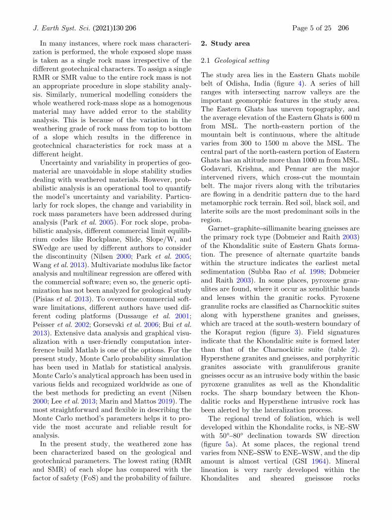
The study area lies in the Eastern Ghats mobilebelt of Odisha, India (Bgure 4). A series of hillranges with intersecting narrow valleys are theimportant geomorphic features in the study area.The Eastern Ghats has uneven topography, andthe average elevation of the Eastern Ghats is 600 mfrom MSL. The north-eastern portion of themountain belt is continuous, where the altitudevaries from 300 to 1500 m above the MSL. Thecentral part of the north-eastern portion of EasternGhats has an altitude more than 1000 m from MSL.Godavari, Krishna, and Pennar are the majorintervened rivers, which cross-cut the mountainbelt. The major rivers along with the tributariesare Cowing in a dendritic pattern due to the hardmetamorphic rock terrain. Red soil, black soil, andlaterite soils are the most predominant soils in theregion.Garnet–graphite–sillimanite bearing gneisses are

the primary rock type (Dobmeier and Raith 2003)of the Khondalitic suite of Eastern Ghats forma-tion. The presence of alternate quartzite bandswithin the structure indicates the earliest metalsedimentation (Subba Rao et al. 1998; Dobmeierand Raith 2003). In some places, pyroxene gran-ulites are found, where it occur as xenolithic bandsand lenses within the granitic rocks. Pyroxenegranulite rocks are classiBed as Charnockitic suitesalong with hypersthene granites and gneisses,which are traced at the south-western boundary ofthe Koraput region (Bgure 3). Field signaturesindicate that the Khondalitic suite is formed laterthan that of the Charnockitic suite (table 2).Hypersthene granites and gneisses, and porphyriticgranites associate with granuliferous granitegneisses occur as an intrusive body within the basicpyroxene granulites as well as the Khondaliticrocks. The sharp boundary between the Khon-dalitic rocks and Hypersthene intrusive rock hasbeen alerted by the lateralization process.The regional trend of foliation, which is well

developed within the Khondalite rocks, is NE–SWwith 50�–80� declination towards SW direction(Bgure 5a). At some places, the regional trendvaries from NNE–SSW to ENE–WSW, and the dipamount is almost vertical (GSI 1964). Minerallineation is very rarely developed within theKhondalites and sheared gneissose rocks


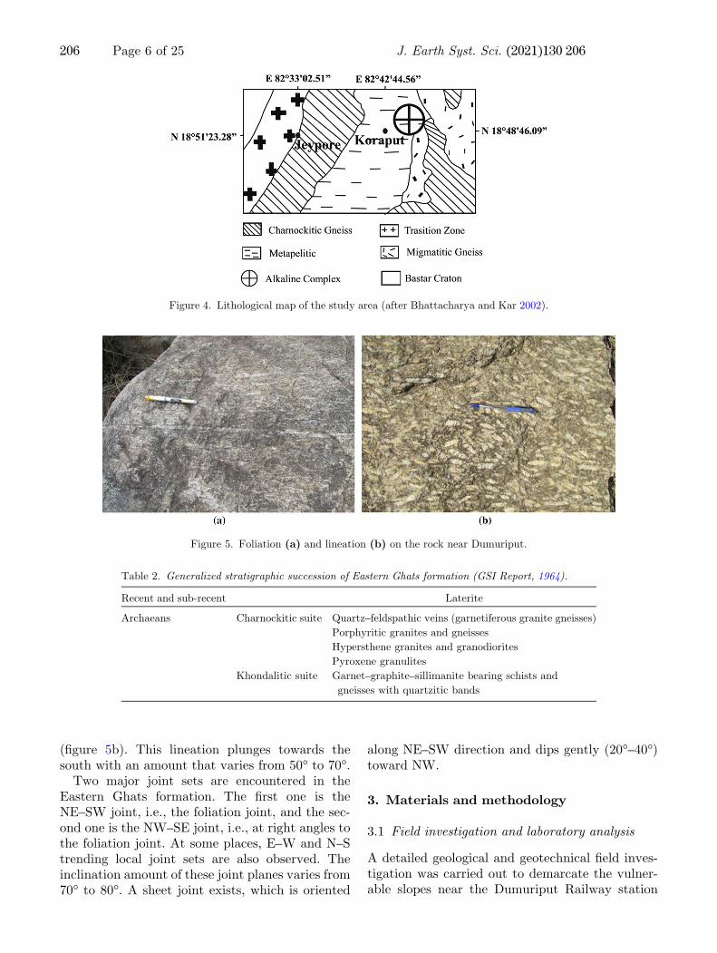
(Bgure 5b). This lineation plunges towards thesouth with an amount that varies from 50� to 70�.Two major joint sets are encountered in the

Eastern Ghats formation. The Brst one is theNE–SW joint, i.e., the foliation joint, and the sec-ond one is the NW–SE joint, i.e., at right angles tothe foliation joint. At some places, E–W and N–Strending local joint sets are also observed. Theinclination amount of these joint planes varies from70� to 80�. A sheet joint exists, which is oriented

along NE–SW direction and dips gently (20�–40�)toward NW.

3. Materials and methodology

3.1 Field investigation and laboratory analysis

A detailed geological and geotechnical Beld inves-tigation was carried out to demarcate the vulner-able slopes near the Dumuriput Railway station

Figure 4. Lithological map of the study area (after Bhattacharya and Kar 2002).

Figure 5. Foliation (a) and lineation (b) on the rock near Dumuriput.

Table 2. Generalized stratigraphic succession of Eastern Ghats formation (GSI Report, 1964).

Recent and sub-recent Laterite

Archaeans Charnockitic suite Quartz–feldspathic veins (garnetiferous granite gneisses)

Porphyritic granites and gneisses

Hypersthene granites and granodiorites

Pyroxene granulites

Khondalitic suite Garnet–graphite–sillimanite bearing schists and

gneisses with quartzitic bands


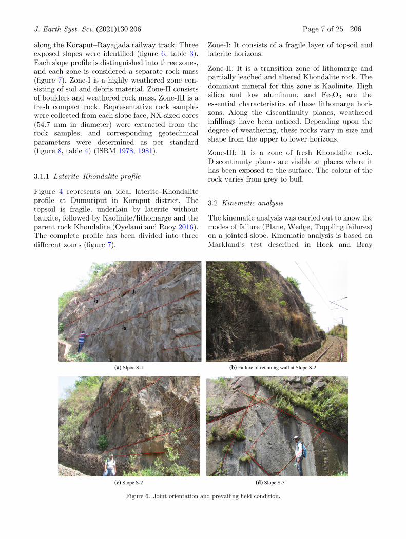
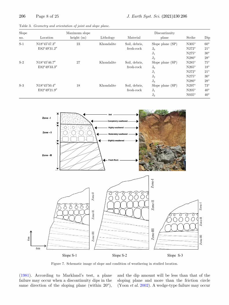
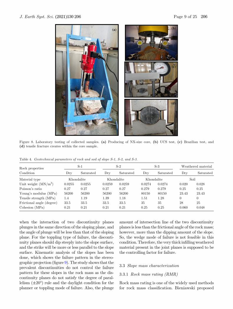
along the Koraput–Rayagada railway track. Threeexposed slopes were identiBed (Bgure 6, table 3).Each slope proBle is distinguished into three zones,and each zone is considered a separate rock mass(Bgure 7). Zone-I is a highly weathered zone con-sisting of soil and debris material. Zone-II consistsof boulders and weathered rock mass. Zone-III is afresh compact rock. Representative rock sampleswere collected from each slope face, NX-sized cores(54.7 mm in diameter) were extracted from therock samples, and corresponding geotechnicalparameters were determined as per standard(Bgure 8, table 4) (ISRM 1978, 1981).

3.1.1 Laterite–Khondalite proBle

Figure 4 represents an ideal laterite–KhondaliteproBle at Dumuriput in Koraput district. Thetopsoil is fragile, underlain by laterite withoutbauxite, followed by Kaolinite/lithomarge and theparent rock Khondalite (Oyelami and Rooy 2016).The complete proBle has been divided into threedifferent zones (Bgure 7).

Zone-I: It consists of a fragile layer of topsoil andlaterite horizons.

Zone-II: It is a transition zone of lithomarge andpartially leached and altered Khondalite rock. Thedominant mineral for this zone is Kaolinite. Highsilica and low aluminum, and Fe2O3 are theessential characteristics of these lithomarge hori-zons. Along the discontinuity planes, weatheredinBllings have been noticed. Depending upon thedegree of weathering, these rocks vary in size andshape from the upper to lower horizons.

Zone-III: It is a zone of fresh Khondalite rock.Discontinuity planes are visible at places where ithas been exposed to the surface. The colour of therock varies from grey to buA.

3.2 Kinematic analysis

The kinematic analysis was carried out to know themodes of failure (Plane, Wedge, Toppling failures)on a jointed-slope. Kinematic analysis is based onMarkland’s test described in Hoek and Bray

(a) Slpoe S-1 (b) Failure of retaining wall at Slope S-2

(c) Slope S-2 (d) Slope S-3

Figure 6. Joint orientation and prevailing Beld condition.


(1981). According to Markland’s test, a planefailure may occur when a discontinuity dips in thesame direction of the sloping plane (within 20�),

and the dip amount will be less than that of thesloping plane and more than the friction circle(Yoon et al. 2002). A wedge-type failure may occur

Slope S-1 Slope S-2 Slope S-3

Figure 7. Schematic image of slope and condition of weathering in studied location.

Table 3. Geometry and orientation of joint and slope plane.

Slope

no. Location

Maximum slope

height (m) Lithology Material

Discontinuity

plane Strike Dip

S-1 N18�45047.300

E82�49031.20023 Khondalite Soil, debris,

fresh-rock

Slope plane (SP) N305� 60�J0 N272� 21�J1 N275� 30�J2 N280� 28�

S-2 N18�45046.700


fresh-rock

Slope plane (SP) N285� 75�J0 N265� 18�J1 N272� 21�J2 N275� 30�J3 N280� 28�

S-3 N18�45050.400


fresh-rock

Slope plane (SP) N297� 73�J1 N205� 40�J2 N035� 40�


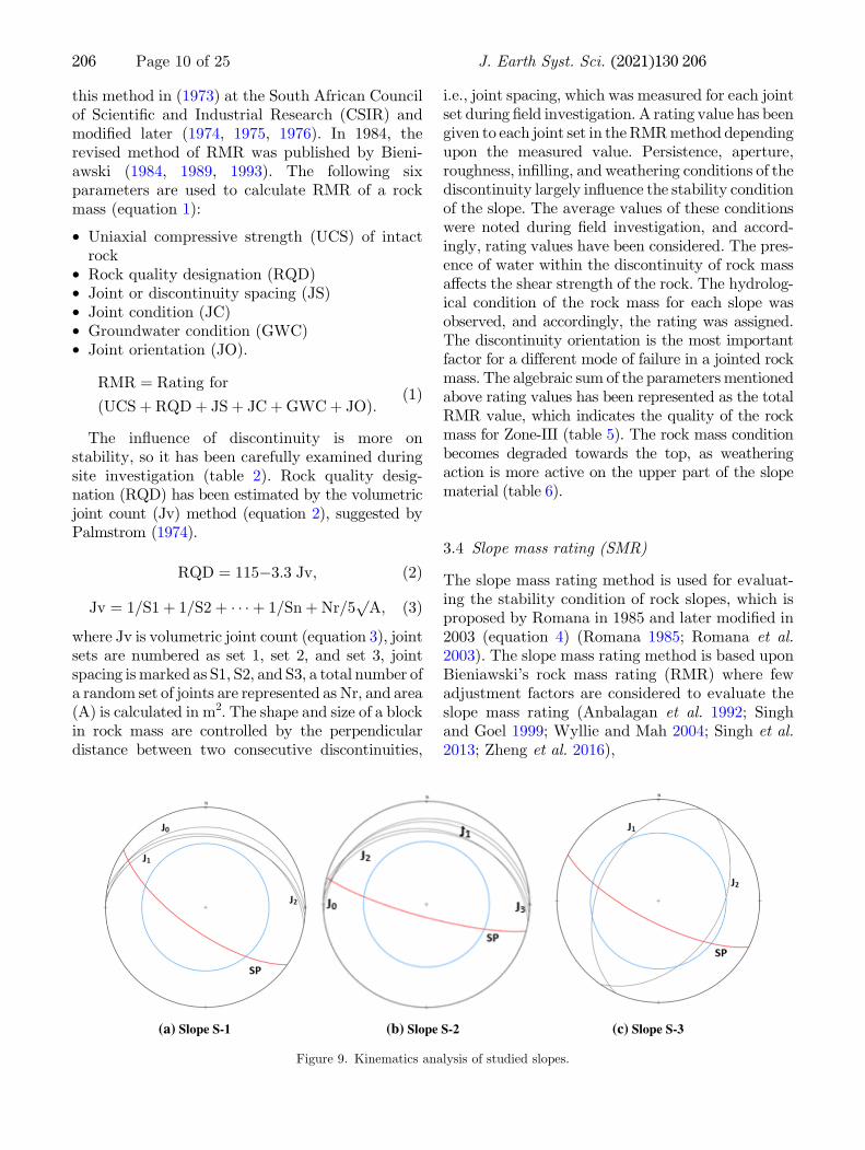
when the interaction of two discontinuity planesplunges in the same direction of the sloping plane, andthe angle of plunge will be less than that of the slopingplane. For the toppling type of failure, the disconti-nuity planes should dip steeply into the slope surface,and the strike will be more or less parallel to the slopesurface. Kinematic analysis of the slopes has beendone, which shows the failure pattern in the stereo-graphic projection (Bgure 9).The study shows that theprevalent discontinuities do not control the failurepattern for these slopes in the rock mass as the dis-continuity planes do not satisfy the degree of paral-lelism (±20�) rule and the daylight condition for theplanner or toppling mode of failure. Also, the plunge

amount of intersection line of the two discontinuityplanes is less than the frictional angle of the rockmass;however, more than the dipping amount of the slope.So, the wedge mode of failure is not feasible in thiscondition.Therefore, thevery thick inBllingweatheredmaterial present in the joint planes is supposed to bethe controlling factor for failure.

3.3 Slope mass characterization

3.3.1 Rock mass rating (RMR)

Rock mass rating is one of the widely used methodsfor rock mass classiBcation. Bieniawski proposed

(a) (b)

(c)

(d)

Figure 8. Laboratory testing of collected samples. (a) Producing of NX-size core, (b) UCS test, (c) Brazilian test, and(d) tensile fracture creates within the core sample.

Table 4. Geotechnical parameters of rock and soil of slope S-1, S-2, and S-3.

Rock propertiesS-1 S-2 S-3 Weathered material

Condition Dry Saturated Dry Saturated Dry Saturated Dry Saturated

Material type Khondalite Khondalite Khondalite Soil

Unit weight (MN/m3) 0.0255 0.0255 0.0259 0.0259 0.0274 0.0274 0.020 0.028

Poisson’s ratio 0.27 0.27 0.27 0.27 0.279 0.279 0.25 0.25

Young’s modulus (MPa) 56200 56200 56200 56200 80150 80150 23.43 23.43

Tensile strength (MPa) 1.4 1.19 1.39 1.18 1.51 1.28 0 0

Frictional angle (degree) 33.5 33.5 33.5 33.5 35 35 28 25

Cohesion (MPa) 0.21 0.21 0.21 0.21 0.25 0.25 0.060 0.048


this method in (1973) at the South African Councilof ScientiBc and Industrial Research (CSIR) andmodiBed later (1974, 1975, 1976). In 1984, therevised method of RMR was published by Bieni-awski (1984, 1989, 1993). The following sixparameters are used to calculate RMR of a rockmass (equation 1):

• Uniaxial compressive strength (UCS) of intactrock

• Rock quality designation (RQD)• Joint or discontinuity spacing (JS)• Joint condition (JC)• Groundwater condition (GWC)• Joint orientation (JO).

RMR ¼ Rating for

UCSþ RQDþ JSþ JCþGWCþ JOð Þ:ð1Þ

The inCuence of discontinuity is more onstability, so it has been carefully examined duringsite investigation (table 2). Rock quality desig-nation (RQD) has been estimated by the volumetricjoint count (Jv) method (equation 2), suggested byPalmstrom (1974).

RQD ¼ 115�3:3 Jv; ð2Þ

Jv ¼ 1=S1þ 1=S2þ � � � þ 1=SnþNr=5pA; ð3Þ

where Jv is volumetric joint count (equation 3), jointsets are numbered as set 1, set 2, and set 3, jointspacing ismarked as S1, S2, and S3, a total number ofa random set of joints are represented as Nr, and area(A) is calculated in m2. The shape and size of a blockin rock mass are controlled by the perpendiculardistance between two consecutive discontinuities,

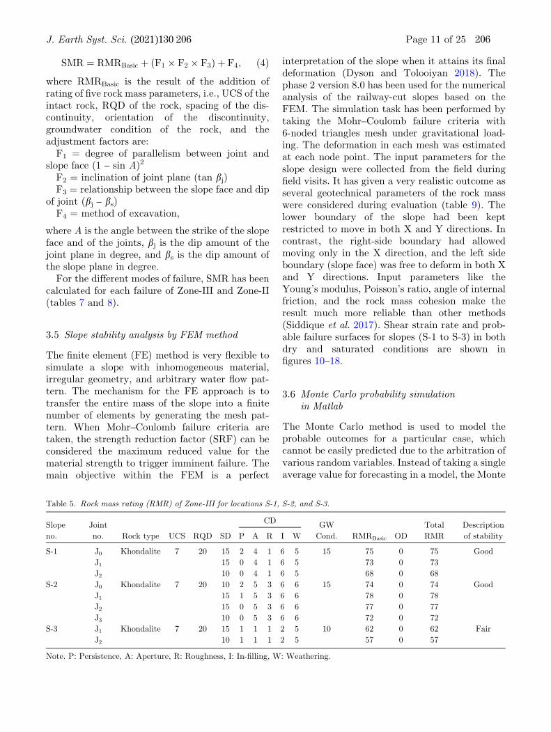
i.e., joint spacing, which was measured for each jointset during Beld investigation. A rating value has beengiven to each joint set in theRMRmethod dependingupon the measured value. Persistence, aperture,roughness, inBlling, and weathering conditions of thediscontinuity largely inCuence the stability conditionof the slope. The average values of these conditionswere noted during Beld investigation, and accord-ingly, rating values have been considered. The pres-ence of water within the discontinuity of rock massaAects the shear strength of the rock. The hydrolog-ical condition of the rock mass for each slope wasobserved, and accordingly, the rating was assigned.The discontinuity orientation is the most importantfactor for a different mode of failure in a jointed rockmass. The algebraic sum of the parameters mentionedabove rating values has been represented as the totalRMR value, which indicates the quality of the rockmass for Zone-III (table 5). The rock mass conditionbecomes degraded towards the top, as weatheringaction is more active on the upper part of the slopematerial (table 6).

3.4 Slope mass rating (SMR)

The slope mass rating method is used for evaluat-ing the stability condition of rock slopes, which isproposed by Romana in 1985 and later modiBed in2003 (equation 4) (Romana 1985; Romana et al.2003). The slope mass rating method is based uponBieniawski’s rock mass rating (RMR) where fewadjustment factors are considered to evaluate theslope mass rating (Anbalagan et al. 1992; Singhand Goel 1999; Wyllie and Mah 2004; Singh et al.2013; Zheng et al. 2016),

(a) Slope S-1 (b) Slope S-2 (c) Slope S-3

Figure 9. Kinematics analysis of studied slopes.


SMR ¼ RMRBasic þ F1 � F2 � F3ð Þ þ F4; ð4Þ

where RMRBasic is the result of the addition ofrating of Bve rock mass parameters, i.e., UCS of theintact rock, RQD of the rock, spacing of the dis-continuity, orientation of the discontinuity,groundwater condition of the rock, and theadjustment factors are:F1 = degree of parallelism between joint and

slope face (1 – sin A)2

F2 = inclination of joint plane (tan bj)F3 = relationship between the slope face and dip

of joint (bj – bs)F4 = method of excavation,

where A is the angle between the strike of the slopeface and of the joints, bj is the dip amount of thejoint plane in degree, and bs is the dip amount ofthe slope plane in degree.For the different modes of failure, SMR has been

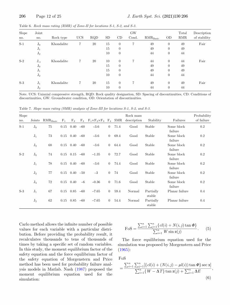
calculated for each failure of Zone-III and Zone-II(tables 7 and 8).

3.5 Slope stability analysis by FEM method

The Bnite element (FE) method is very Cexible tosimulate a slope with inhomogeneous material,irregular geometry, and arbitrary water Cow pat-tern. The mechanism for the FE approach is totransfer the entire mass of the slope into a Bnitenumber of elements by generating the mesh pat-tern. When Mohr–Coulomb failure criteria aretaken, the strength reduction factor (SRF) can beconsidered the maximum reduced value for thematerial strength to trigger imminent failure. Themain objective within the FEM is a perfect

interpretation of the slope when it attains its Bnaldeformation (Dyson and Tolooiyan 2018). Thephase 2 version 8.0 has been used for the numericalanalysis of the railway-cut slopes based on theFEM. The simulation task has been performed bytaking the Mohr–Coulomb failure criteria with6-noded triangles mesh under gravitational load-ing. The deformation in each mesh was estimatedat each node point. The input parameters for theslope design were collected from the Beld duringBeld visits. It has given a very realistic outcome asseveral geotechnical parameters of the rock masswere considered during evaluation (table 9). Thelower boundary of the slope had been keptrestricted to move in both X and Y directions. Incontrast, the right-side boundary had allowedmoving only in the X direction, and the left sideboundary (slope face) was free to deform in both Xand Y directions. Input parameters like theYoung’s modulus, Poisson’s ratio, angle of internalfriction, and the rock mass cohesion make theresult much more reliable than other methods(Siddique et al. 2017). Shear strain rate and prob-able failure surfaces for slopes (S-1 to S-3) in bothdry and saturated conditions are shown inBgures 10–18.

3.6 Monte Carlo probability simulationin Matlab

The Monte Carlo method is used to model theprobable outcomes for a particular case, whichcannot be easily predicted due to the arbitration ofvarious random variables. Instead of taking a singleaverage value for forecasting in a model, the Monte

Table 5. Rock mass rating (RMR) of Zone-III for locations S-1, S-2, and S-3.

Slope

no.

Joint

no. Rock type UCS RQD SD

CDGW

Cond. RMRBasic OD

Total

RMR

Description

of stabilityP A R I W

S-1 J0 Khondalite 7 20 15 2 4 1 6 5 15 75 0 75 Good

J1 15 0 4 1 6 5 73 0 73

J2 10 0 4 1 6 5 68 0 68

S-2 J0 Khondalite 7 20 10 2 5 3 6 6 15 74 0 74 Good

J1 15 1 5 3 6 6 78 0 78

J2 15 0 5 3 6 6 77 0 77

J3 10 0 5 3 6 6 72 0 72

S-3 J1 Khondalite 7 20 15 1 1 1 2 5 10 62 0 62 Fair

J2 10 1 1 1 2 5 57 0 57

Note. P: Persistence, A: Aperture, R: Roughness, I: In-Blling, W: Weathering.


Carlo method allows the inBnite number of possiblevalues for each variable with a particular distri-bution. Before providing the probability result, itrecalculates thousands to tens of thousands oftimes by taking a speciBc set of random variables.In this study, the moment equilibrium factor of thesafety equation and the force equilibrium factor ofthe safety equation of Morgenstern and Pricemethod has been used for probability failure anal-ysis models in Matlab. Nash (1987) proposed themoment equilibrium equation used for thesimulation:

FoS ¼Pn

i¼1

Pnj¼1 cl ið Þ þN i; jð Þ tanUf gPn

i¼1W sin a jð Þ : ð5Þ

The force equilibrium equation used for thesimulation was proposed by Morgenstern and Price(1965):

FoS

¼Pn

i¼1

Pnj¼1 cl ið Þ þ N i; jð Þ � ll ið Þð Þ tanUf g sec a½ �

Pni¼1 W � DTf g tan a jð Þ þ

Pni¼1 DE

;

ð6Þ

Table 6. Rock mass rating (RMR) of Zone-II for locations S-1, S-2, and S-3.

Slope

no.

Joint

no. Rock type UCS RQD SD CD

GW

Cond. RMRBasic OD

Total

RMR

Description

of stability

S-1 J0 Khondalite 7 20 15 0 7 49 0 49 Fair

J1 15 0 49 0 49

J2 10 0 44 0 44

S-2 J-1 Khondalite 7 20 10 0 7 44 0 44 Fair

J0 15 0 49 0 49

J1 15 0 49 0 49

J2 10 0 44 0 44

S-3 J1 Khondalite 7 20 15 0 7 49 0 49 Fair

J2 10 0 44 0 44

Note. UCS: Uniaxial compressive strength, RQD: Rock quality designation, SD: Spacing of discontinuities, CD: Conditions ofdiscontinuities, GW: Groundwater condition, OD: Orientation of discontinuities.

Table 7. Slope mass rating (SMR) analysis of Zone-III for locations S-1, S-2, and S-3.

Slope

no. Joints RMRBasic F1 F2 F3 F19F29F3 F4 SMR

Rock mass

description Stability Failures

Probability

of failure

S-1 J0 75 0.15 0.40 –60 –3.6 0 71.4 Good Stable Some block

failure

0.2

J1 73 0.15 0.40 –60 –3.6 0 69.4 Good Stable Some block

failure

0.2


failure

0.2

S-2 J0 74 0.15 0.15 –60 –1.35 0 72.7 Good Stable Some block

failure

0.2


failure

0.2

J2 77 0.15 0.40 –50 –3 0 74 Good Stable Some block

failure

0.2


failure

0.2

S-3 J1 67 0.15 0.85 –60 –7.65 0 59.4 Normal Partially

stable

Planar failure 0.4

J2 62 0.15 0.85 –60 –7.65 0 54.4 Normal Partially

stable

Planar failure 0.4


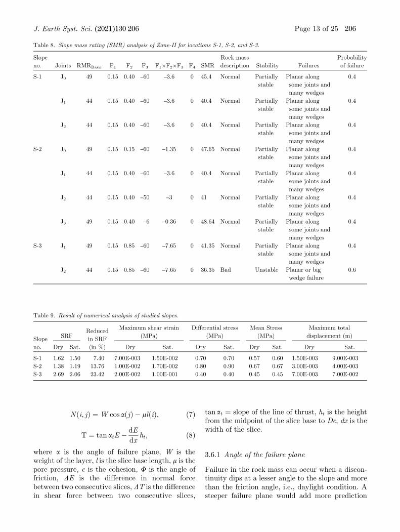
N i; jð Þ ¼ W cos a jð Þ � ll ið Þ; ð7Þ

T ¼ tan atE � dE

dxht; ð8Þ

where a is the angle of failure plane, W is theweight of the layer, l is the slice base length, l is thepore pressure, c is the cohesion, U is the angle offriction, DE is the difference in normal forcebetween two consecutive slices, DT is the differencein shear force between two consecutive slices,

tan at = slope of the line of thrust, ht is the heightfrom the midpoint of the slice base to De, dx is thewidth of the slice.

3.6.1 Angle of the failure plane

Failure in the rock mass can occur when a discon-tinuity dips at a lesser angle to the slope and morethan the friction angle, i.e., daylight condition. Asteeper failure plane would add more prediction

Table 8. Slope mass rating (SMR) analysis of Zone-II for locations S-1, S-2, and S-3.

Slope

no. Joints RMRBasic F1 F2 F3 F19F29F3 F4 SMR

Rock mass

description Stability Failures

Probability

of failure


stable

Planar along

some joints and

many wedges

0.4


stable

Planar along

some joints and

many wedges

0.4


stable

Planar along

some joints and

many wedges

0.4


stable

Planar along

some joints and

many wedges

0.4


stable

Planar along

some joints and

many wedges

0.4

J2 44 0.15 0.40 –50 –3 0 41 Normal Partially

stable

Planar along

some joints and

many wedges

0.4


stable

Planar along

some joints and

many wedges

0.4


stable

Planar along

some joints and

many wedges

0.4

J2 44 0.15 0.85 –60 –7.65 0 36.35 Bad Unstable Planar or big

wedge failure

0.6

Table 9. Result of numerical analysis of studied slopes.

Slope

no.

SRFReduced

in SRF

(in %)

Maximum shear strain

(MPa)

Differential stress

(MPa)

Mean Stress

(MPa)

Maximum total

displacement (m)

Dry Sat. Dry Sat. Dry Sat. Dry Sat. Dry Sat.

S-1 1.62 1.50 7.40 7.00E-003 1.50E-002 0.70 0.70 0.57 0.60 1.50E-003 9.00E-003

S-2 1.38 1.19 13.76 1.00E-002 1.70E-002 0.80 0.90 0.67 0.67 3.00E-003 4.00E-003

S-3 2.69 2.06 23.42 2.00E-002 1.00E-001 0.40 0.40 0.45 0.45 7.00E-003 7.00E-002


sequences for the failure of the rock slope. Hence,due to significant inCuence of the angle of failure onthe safety factor, it has been taken as a vectorquantity for the probability analysis with randomdistribution.

3.6.2 The base length of the slice

Apart from the angle of the failure plane, thelength of the rock mass slice also significantlycontrolled the failure mechanism due to itsdimension factor. The failure probability willincrease with the increase in the dimension of therock mass’s failure. Due to its significant inCuence,this parameter is also taken as a vector quantity forthe analysis.

3.6.3 Pore water pressure

Pore water pressure is described as the pressureexerted by the inBltrated rainwater within theslope. Pore pressure will be maximum when therock mass is fully saturated. Moreover, the min-imum or zero pore pressure will be exerted at thecomplete dry condition. The most common situ-ation will lie in between dry and fully saturatedconditions. For better illustration within theprobability model, pore water pressure isdescribed as a vector quantity with randomdistribution.

3.6.4 Cohesion

Cohesion is the inherent property of the weatheredrock mass. Completely weathered or fresh rockmass and different saturation conditions, coherencehas been taken as an independent variable for theprobability model. A uniform random distributionhas been assigned to the cohesion parameter todeBne the variability. The minimum and maximumvalues for the cohesion have been taken from thelaboratory analysis for each slope.

3.6.5 The angle of internal friction

The angle of internal friction is also described asthe inherent properties of the rock mass. Dependsupon the saturation condition and weatheringcondition, the value mostly lies in between a rangeof maximum to a minimum amount obtained dur-ing the laboratory analysis. As its inCuence is

independent of other parameters, it has been takenas a uniform distribution variable for the proba-bility analysis model.

3.6.6 Normal force

Normal force acting on each slice has been esti-mated for all possibilities. Depending upon theother physical parameters, it varies for each slice.Minimum and maximum reasonable force for allthe slopes are listed in table 10. The difference innormal force had been taken as a vector quantity toillustrate a particular number of failure sliceswithin the probability of the failure zone. More-over, for the distribution of normal force, the nor-mal distribution has been used for bettersimulation results.

3.6.7 Shear force

Shear force for each slice was calculated by usingequation (8). The difference in shear force amongslices is also taken as a vector quantity for theprobability analysis of the force equilibrium prob-ability model. Parameters like normal force, theheight of slice, angle of thrust, and width of theslice, which control the shear force, were measuredand noted in table 10. All these parameters aredistributed normally, which suggested normaldistribution for shear force too.

4. Result

4.1 Dynamic analysis

4.1.1 Slope S-1

Rock mass classiBcation has been done for bothZone-II and Zone-III. The weathering processexponentially degraded the rock mass quality, i.e.,the RMR value for Zone-III is 68–75, whereas forZone-II, it is 44–49 (tables 5 and 6). SMR valueindicates the slope is stable-to-partially stable. Thekinematic analysis has concluded that the slope isnot structurally controlled, as the joint sets dip inthe opposite direction of the slope face at a lesserangle.The FEM shows a different result. Laterite soil

and lithomarge in Zone-II of a laterite–KhondaliteproBle have aAected the stability of the boulders ordifferent sizes and shapes of rock fragments presentin that zone. A circular weak-zone is created at


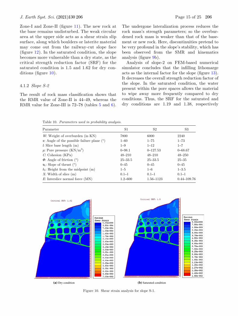
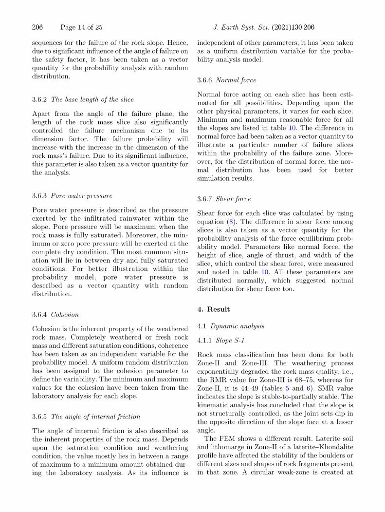
Zone-I and Zone-II (Bgure 11). The new rock atthe base remains undisturbed. The weak circulararea at the upper side acts as a shear strain slipsurface, along which boulders or laterite materialmay come out from the railway-cut slope face(Bgure 12). In the saturated condition, the slopebecomes more vulnerable than a dry state, as thecritical strength reduction factor (SRF) for thesaturated condition is 1.5 and 1.62 for dry con-ditions (Bgure 10).

4.1.2 Slope S-2

The result of rock mass classiBcation shows thatthe RMR value of Zone-II is 44–49, whereas theRMR value for Zone-III is 72–78 (tables 5 and 6).

The undergone lateralization process reduces therock mass’s strength parameters; so the overbur-dened rock mass is weaker than that of the base-ment or new rock. Here, discontinuities pretend tobe very profound in the slope’s stability, which hasbeen observed from the SMR and kinematicsanalysis (Bgure 9b).Analysis of slope-2 on FEM-based numerical

simulator concludes that the inBlling lithomargeacts as the internal factor for the slope (Bgure 13).It decreases the overall strength reduction factor ofthe slope. In the saturated condition, the waterpresent within the pore spaces allows the materialto wipe away more frequently compared to dryconditions. Thus, the SRF for the saturated anddry conditions are 1.19 and 1.38, respectively

Table 10. Parameters used in probability analysis.

Parameter S1 S2 S3

W: Weight of overburden (in KN) 7800 6000 2240

a: Angle of the possible failure plane (�) 1–60 1–75 1–73

l: Slice base length (m) 1–9 1–12 1–7

l: Pore pressure (KN/m3) 0–98.1 0–127.53 0–68.67

C: Cohesion (KPa) 48–210 48–210 48–250

U: Angle of friction (�) 25–33.5 25–33.5 25–35

at: Slope of thrust (�) 0–45 0–45 0–45

ht: Height from the midpoint (m) 1–5 1–6 1–3.5

X: Width of slice (m) 0.1–1 0.1–1 0.1–1

E: Interslice normal force (MN) 1.2–600 1.56–1123 0.44–109.76

(a) Dry condition (b) Saturated condition

Figure 10. Shear strain analysis for slope S-1.


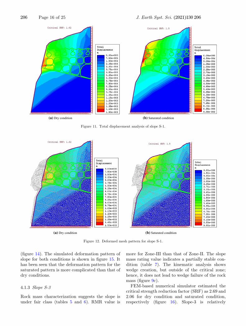
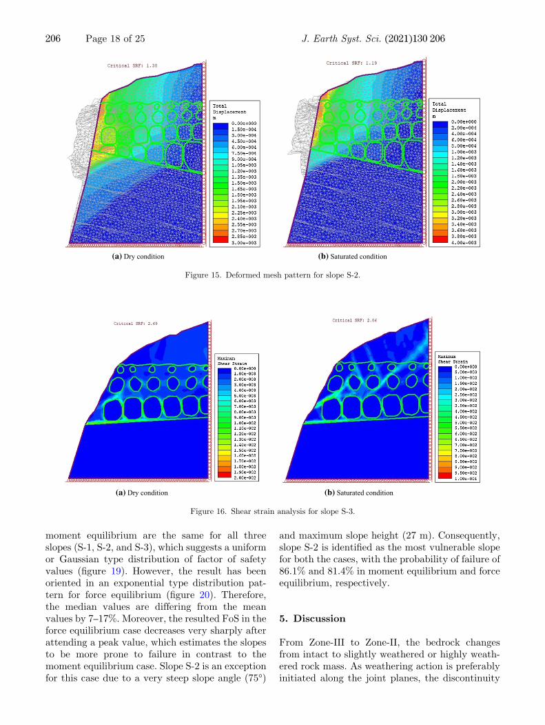
(Bgure 14). The simulated deformation pattern ofslope for both conditions is shown in Bgure 15. Ithas been seen that the deformation pattern for thesaturated pattern is more complicated than that ofdry conditions.

4.1.3 Slope S-3

Rock mass characterization suggests the slope isunder fair class (tables 5 and 6). RMR value is

more for Zone-III than that of Zone-II. The slopemass rating value indicates a partially stable con-dition (table 7). The kinematic analysis showswedge creation, but outside of the critical zone;hence, it does not lead to wedge failure of the rockmass (Bgure 9c).FEM-based numerical simulator estimated the

critical strength reduction factor (SRF) as 2.69 and2.06 for dry condition and saturated condition,respectively (Bgure 16). Slope-3 is relatively


Figure 11. Total displacement analysis of slope S-1.


Figure 12. Deformed mesh pattern for slope S-1.


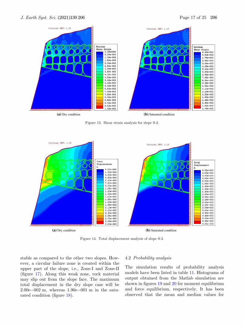
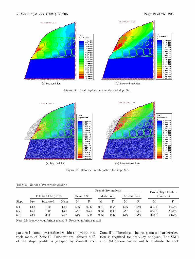
stable as compared to the other two slopes. How-ever, a circular failure zone is created within theupper part of the slope, i.e., Zone-I and Zone-II(Bgure 17). Along this weak zone, rock materialmay slip out from the slope face. The maximumtotal displacement in the dry slope case will be2.00e�002 m, whereas 1.90e�001 m in the satu-rated condition (Bgure 18).

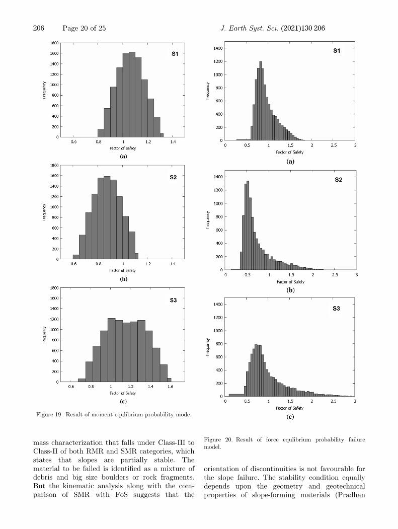
4.2 Probability analysis

The simulation results of probability analysismodels have been listed in table 11. Histograms ofoutput obtained from the Matlab simulation areshown in Bgures 19 and 20 for moment equilibriumand force equilibrium, respectively. It has beenobserved that the mean and median values for






moment equilibrium are the same for all threeslopes (S-1, S-2, and S-3), which suggests a uniformor Gaussian type distribution of factor of safetyvalues (Bgure 19). However, the result has beenoriented in an exponential type distribution pat-tern for force equilibrium (Bgure 20). Therefore,the median values are differing from the meanvalues by 7–17%. Moreover, the resulted FoS in theforce equilibrium case decreases very sharply afterattending a peak value, which estimates the slopesto be more prone to failure in contrast to themoment equilibrium case. Slope S-2 is an exceptionfor this case due to a very steep slope angle (75�)

and maximum slope height (27 m). Consequently,slope S-2 is identiBed as the most vulnerable slopefor both the cases, with the probability of failure of86.1% and 81.4% in moment equilibrium and forceequilibrium, respectively.

5. Discussion

From Zone-III to Zone-II, the bedrock changesfrom intact to slightly weathered or highly weath-ered rock mass. As weathering action is preferablyinitiated along the joint planes, the discontinuity






pattern is somehow retained within the weatheredrock mass of Zone-II. Furthermore, almost 80%of the slope proBle is grasped by Zone-II and

Zone-III. Therefore, the rock mass characteriza-tion is required for stability analysis. The SMRand RMR were carried out to evaluate the rock





Table 11. Result of probability analysis.

Slope

FoS by FEM (SRF)

Probability analysisProbability of failure

(FoS\ 1)Mean FoS Mode FoS Median FoS

Dry Saturated Mean M F M F M F M F

S-1 1.62 1.50 1.56 1.06 0.96 0.81 0.58 1.06 0.89 30.7% 66.2%

S-2 1.38 1.19 1.28 0.87 0.74 0.62 0.33 0.87 0.61 86.1% 81.4%

S-3 2.69 2.06 2.37 1.16 1.00 0.72 0.42 1.16 0.86 24.5% 64.2%

Note. M: Moment equilibrium model, F: Force equilibrium model.


mass characterization that falls under Class-III toClass-II of both RMR and SMR categories, whichstates that slopes are partially stable. Thematerial to be failed is identiBed as a mixture ofdebris and big size boulders or rock fragments.But the kinematic analysis along with the com-parison of SMR with FoS suggests that the

orientation of discontinuities is not favourable forthe slope failure. The stability condition equallydepends upon the geometry and geotechnicalproperties of slope-forming materials (Pradhan

Figure 19. Result of moment equlibrium probability mode.

Figure 20. Result of force equlibrium probability failuremodel.


et al. 2018; Komadja et al. 2020; Niyogi et al.2020). Therefore, rock mass characterizationshould not be a single tool in the estimation ofstability analysis. RMR and SMR estimate theslope mass condition without a quantitativedescription of the stability condition of the slope,such as FoS. However, in the numerical simula-tion tool, both geometries and material propertiesof the slope are required to calculate the factor ofsafety. Therefore, FoS was estimated by the FEmodel and probabilistic equilibrium models byconsidering the parameters of each zone(Bgures 10–20). The rock mass characterization

of Zone-II and Zone-III suggests the weatheringdegrades the condition of the rock mass. Zone-IIcontains a very thick layer of weathered massalong its joint planes. It results in Zone-II beingmore vulnerable than Zone-III and can favour theinitiation of failure mechanism irrespective of thejoint condition. Hence, the rating values of rockmass characterization are not always directlylinked to the factor of safety. In this study, slopeS-3 has the lowest RMR and SMR values.However, the strength reduction factor or FoS ismaximum for S-3, among the slopes, due to itslesser height than the other two slopes as lowerheight slopes are less vulnerable for failure incomparison to the higher slopes (Solanki et al.2019; Siddique et al. 2020). Relative relief orheight of the slope is one of the crucial parame-ters that inCuenced the overall stability of theslopes (Pantelidis 2009; Pradhan et al. 2011;Acharya et al. 2020; Pradhan and Siddique2020). The inBlling material and weathered massplay a vital role in the failure of a slope. Due tothe lateralization process, the formation of thelithomarge horizon within Zone-I and Zone-IIcauses the abundant presence of Kaolinite withinthe rock mass in the Ghats region of India(Deepthy and Balakrishnan 2005; Jean et al.2019). With the increase in water content, theexpansion of Kaolinite exerts lateral forces on thesurrounding material, which reduces the overallshear strength of the rock mass (Collins andZnidarcic 2004; Peckley et al. 2010). Thus, theslope becomes more vulnerable even after highRMR and SMR ratings.The SRF values of all the investigated slopes are

given in table 9. It has been seen that S-2 is morevulnerable to failure in comparison to S-1 and S-3slopes. Compared to the dry condition, theStrength Reduction Factor is decreased by almost10–20% in the saturated state. The S-2 railway-cutslope is relatively steeper, which aAects the sta-bility condition of the material present on the slopeface. In the S-3 slope, due to shorter height, theSRF is relatively high although the rock mass isweak.For the stability assessment, the FoS has been

calculated and compared with the probability offailure for different equilibrium models. However,several studies have pointed out that the FoS fac-tor is a random variable when various uncertaintiesare incorporated into the analysis (Smith 2003).Therefore, the probability of failure becomes aprobability function of the FoS, i.e., P(FoS \ 1)

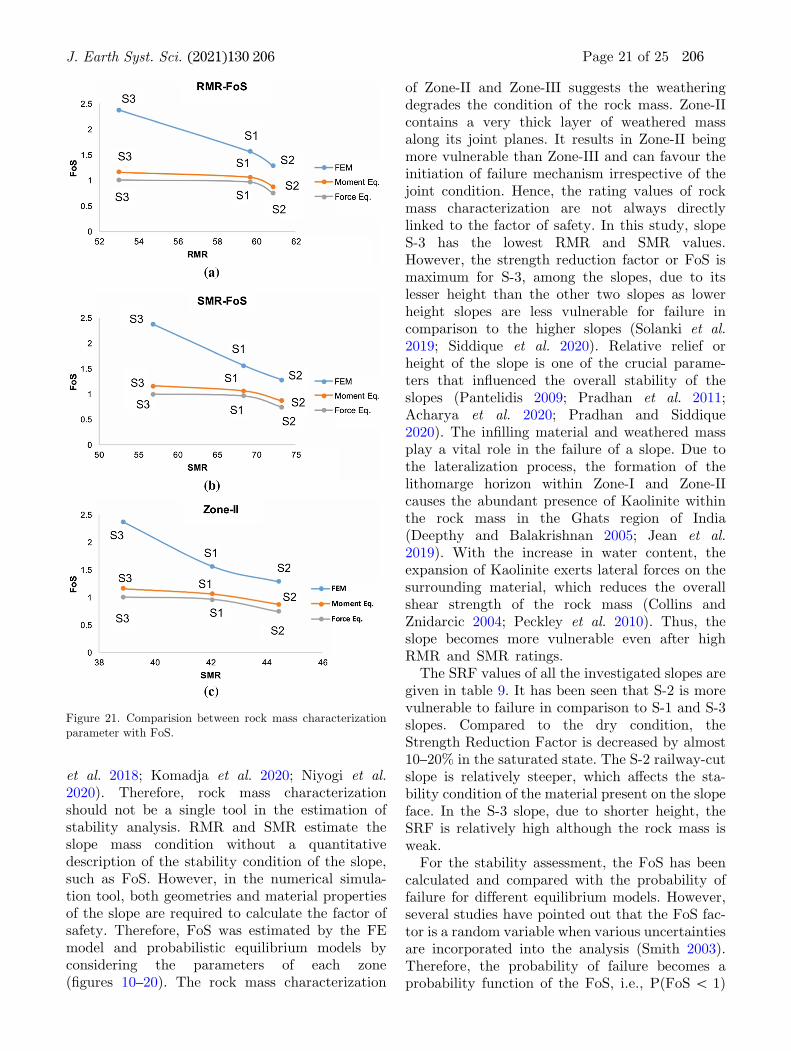
Figure 21. Comparision between rock mass characterizationparameter with FoS.


(Altareios-Garcia et al. 2012). In general, with theincrease of FoS value, the probability of failuredecreases; however, Smith (2003) and Silva et al.(2008) proved that the relationship is not directlyproportional always. Uncertainties present in theanalysis, such as uncertainty in input parameters,system uncertainty, and loading uncertainty, donot lead the probability of failure to lower for everyrise in FoS values. Hence, the probability analysisis essential to enhance the outcomes derived fromthe stability analysis integrated with the FEmethod.Rock mass condition inCuences the stability of

the slope (Siddque and Pradhan 2018); however,the inCuence has been varying for each proba-bility model and FE model. Javankhoshdel andBathurst (2017) stated that even similar slopesmay have the same FoS, but may result in dif-ferences in failure probability. In Bgure 21, theestimated FoS using the probability models andBnite element model has been correlated with therock mass characterization (RMR and SMR). Forboth models, the FoS is inversely correlated withthe rock mass condition. So, slope S-2 showsminimum FoS for all the models even afterhaving better rock mass conditions. According tothe FEM of the studied slopes, the probablefailure surface of each slope is lying in Zone-I andZone-II only. However, for detailed analysis, FoSof the slope has been compared with the meanRMR and SMR of Zone-II and Zone-III for eachslope. There is no direct relation between thestability factors and the rock mass condition(RMR and SMR) for a weathered slope. Thethick layer of the weathered mass present alongthe joints in Zone-II and the completely weath-ered material of Zone-I are responsible fordecreasing the stability of the weathered slopes.In stability analysis model, both rock mass

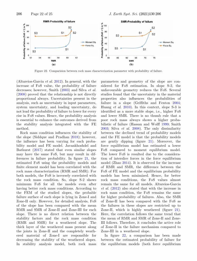
parameters and geometry of the slope are con-sidered for FoS estimation. In slope S-2, theunfavourable geometry reduces the FoS. Severalstudies found that the uncertainty in the materialproperties also inCuences the probabilities offailure in a slope (GrifBths and Fenton 2004;Huang et al. 2010). In this context, slope S-3 isidentiBed as a more stable slope, i.e., higher FoSand lower SMR. There is no thumb rule that apoor rock mass always shows a higher proba-bilistic of failure (Hassan and WolA 1999; Smith2003; Silva et al. 2008). The only dissimilaritybetween the declined trend of probability modelsand the FE model is that the probability modelsare gently dipping (Bgure 21). Moreover, theforce equilibrium model has estimated a lowerFoS compared to moment equilibrium model.The lower FoS is resulted due to the considera-tion of interslice forces in the force equilibriummodel (Zhao 2014). It is observed for the increaseof RMR and SMR, the difference between theFoS of FE model and the equilibrium probabilitymodels has been minimized. Hence, for betterrock mass conditions, the FoS values almostremain the same for all models. Altareios-Garciaet al. (2012) also stated that with the increase inrock mass condition, the FoS remains the samefor higher probability of failures. Also, the SMRof Zone-II has been compared with the FoS asthe failures in these slopes are restricted up toZone-II, which is highly weathered (Bgure 21).Here, the correlation follows the same trend thatthe mean of RMR and SMR of Zone-II and Zone-III follows. Therefore, it concludes the active roleof Zone-II in the failure mechanism compared toZone-III in a weathered slope.In Bgure 22, a comparison has been made

between the estimated probability of failure forthe equilibrium models (both force equilibrium

Figure 22. Comparision between rock mass characterization parameter with probability of failure.


and moment equilibrium) and the rock masscondition (RMR and SMR). It is observed thatthe probability of failure for the force equilibriummodel is relatively high. However, for slope S-2,the estimated probability of failure for both theequilibrium models is almost identical. As in theprevious paragraph, it has been mentioned thatthe FoS estimated by the equilibrium models forthe good rock mass condition is nearly equal. Butthe unfavourable geometry and the presence ofweathered material at Zone-I and Zone-II makethe slope S-2 more vulnerable to failure (GrifBthsand Fenton 2004; Huang et al. 2010). It results inthe probability of failure models of slope S-2 todiffer very slightly from each other. Hence, it canbe concluded that the presence of fresh rock atthe bottom (Zone-III) improves the overall ratingof the rock mass condition of the slope. However,the weathered mass present at Zone-I and Zone-II reduces the FoS of the slope.

6. Conclusion

From the above rock mass classiBcation andnumerical analysis, it has been observed that theheight and slope angle have a significant role inthe failure of the slope. The rock mass seemsreasonable, but numerical modelling shows thatthe slope may fail along the probable slip surface.The results are corroborated with the prevailingBeld condition, as in the case of S-2. In slope S-2,although the slopes’ SMR is relatively high, thelaterite soil presents above the fresh rock, andthe thick layer of weathered mass along the jointplanes has inCuenced the overall shear strengthof the slope. The strength reduction factor (SRF)value for the saturated condition has decreasedby up to 10% compared to that of dry conditions.After heavy precipitation, slopes become morevulnerable due to the reduction of shear strengthparameter. Failure surface generated withinZone-II is expected to be the most sensitive zonefor initiating or rolling boulders. Therefore, irre-spective of the joint orientation, the probablefailure surface in Zone-I initiates and moves upto Zone-II without invading Zone-III. It can alsobe concluded from kinematic analysis that theslope failures along the railway track is notstructurally controlled. The factor of safetyobtained from the numerical simulation is notdirectly related to RMR or SMR of the slopemass.

Author statement

Amulya Ratna Roul: Conceived, designed andperformed the experiments; collected, analysed andinterpreted the data; contributed materials, anal-ysis tools; performed writing. Sarada PrasadPradhan: Conceived and designed the experiments;analyzed and interpreted the data; contributedmaterials, analysis tools and data; and performedwriting – review and editing. Durga PrasannaMohanty: Collected Beld sample, analyzed andinterpreted the data, performed review.

References

Acharya B, Sarkar K, Singh A K and Chawla S 2020Preliminary slope stability analysis and discontinuitiesdriven susceptibility zonation along a crucial highwaycorridor in higher Himalaya India; J. Mt. Sci. 17(4)801–823.

Altareios-Garcia L, Escuder-Bueno I, Serrano-Lombillo A andMorales-Torres A 2012 Factor of safety and probability offailure in concrete dams; In: Risk Analysis, Dam Safety,Dam Security and Critical Infrastructure Management(eds) Escuder-Bueno et al., Taylor & Francis Group,London.

Anbalagan R, Sharma S and Raghuvanshi T K 1992 Rockmass stability evaluation using modiBed SMR approach;Proc. 6th Natl. Symp. Rock Mech. 1 258–268.

Balaji P, Pavanaguru R and Reddy D V 2010 A note on theoccurrence of landslides in Araku valley and its environs,Visakhapatnam District, Andhra Pradesh, India; Int. EarthSci. Eng. 3 13–19.

Bhattacharya S and Kar R 2002 High-temperature dehydra-tion melting and decompressive P-T path in a granulitecomplex from Eastern Ghats, India; Contrib. Mineral.Petrol. 143 175–191.

Bieniawski Z T 1973 Engineering classiBcation of jointed rockmasses; South African Inst. Civil Eng. 15 335–344.

Bieniawski Z T 1974 Geomechanics classiBcation of rockmasses and its application in tunnelling; Adv. RockMechanics, Proc. of 3rd Cong. of ISRM, National Acad.Sci., Washington, D.C. II(A) 27–30.

Bieniawski Z T 1975 Case studies: Prediction of rock massesbehaviour by geomechanics classiBcation; Proc. of 2ndAustralia–New Zealand Conf. Geomech. Brisbane,pp. 36–41.

Bieniawski Z T 1976 Rock mass classiBcations in engineering;Proc. Symp. Expl. Rock Eng. Johensberg, pp. 97–106.

Bieniawski Z T 1984 Rock Mechanics Design in Mining andTunnelling; A.A Balkema, Rotterdam.

Bieniawski Z T 1989 Engineering Rock Mass ClassiBcations;Wiley, New York.

Bieniawski Z T 1993 ClassiBcation of rock masses forengineering: The RMR system and future trends; In: RockTesting and Site Characterization, Pergamon Press,Oxford, UK, pp. 553–573.

Bisop A W 1955 The use of the slip circle in the stabilityanalysis of slopes; Geotechnique 5(1) 7–17.


Bui D T, Pradhan B, Lofman O, Revhaug I and Dick Q B 2013Regional prediction of landslide hazard using probabilityanalysis of intense rainfall in the Hoa Binh province,Vietnam; Nat. Hazards 66 707–730.

Cheng Y M, Lansivaara T and Wei W B 2007 Two-dimensionalslope stability analysis by limit equilibrium and strengthreduction methods; Comput. Geotech. 34 137–150.

Chowdary T S R, Prasad K S R and Ram Babu T S 2015Geotechnical characterization of weathered Khondalitezones, Indrakheeladri Hills, Vijayawada, Andhra Pradesh,India; Int. J. Eng. Tech. Mgmt. Appl. Sci. 3 199–206.

Collins B D and Znidarcic D 2004 Stability analyses of rainfallinduced landslides; J. Geotech. Geoenviron. 130 362–372.

Das I, Sahoo S, Van Weston C, Stein A and Hack R 2010Landslide susceptibility assessment using logistic regressionand its comparison with a rock mass classiBcation system,along a road section in the northern Himalayas (India);Geomorphology 114 741–765.

Deepthy R and Balakrishnan S 2005 Climatic control on claymineral formation: evidence from weathering proBles devel-oped on either side of the Western Ghats; J. Earth Syst. Sci.114(5) 545–556.

Dobmeier C J and Raith M M 2003 Crustal architecture andevolution of the Eastern Ghats belt and adjacent region ofIndia; Geol. Soc. London Memoir Spec. Publ. 206145–168.

Dussauge C, Grasso J and Helmstetter A 2001 Statisticalanalysis of rock falls: Implication for hazard assessment andunderlying physical processes; J. Geophys. Res. 108 1–11.

Dyson A P and Tolooiyan A 2018 Optimization of strengthreduction Bnite element method codes for slope stabilityanalysis; Innov. Infrastruct. Solut. 3 1–12.

Eberhardt E, Stead D and Coggan J S 2004 Numerical analysisof initiation and progressive failure in natural rock slopes –the 1991 Randa rockslide; Int J. Rock Mech. Min. Sci. 4169–87.

Gorsevski P V, Foltz R B, Gessler P E and Elliot W J 2006Spatial prediction of landslide hazard using logistic regres-sion and ROC analysis; Trans GIS 10(3) 395–415.

GrifBths D V and Lane P A 1999 Slope stability analysis byBnite elements; Geotechnique 49 387–403.

GrifBths D V and Fenton G A 2004 Probabilistic slopestability analysis by Bnite elements; J. Geotech. Geoenvi-ron. 130(5) 507–518.

GrifBths D V 2015 Slope stability analysis by Bnite elements;Geomechanics Research Centre, Colorado School of Mines.

GSI Progress Report 1964 Report on systematic geologicalmapping in parts of Koraput District, Orissa.

Hassan A M and WolA T F 1999 Search algorithm forminimum reliability index of earth slope; J. Geotech.Geoenviron. 125(4) 301–308.

Hoek E and Bray J 1981 Rock Slope Engineering; 3rd edn. TheInstitution of Mining and Metallurgy, London.

Huang J, GrifBths D V and Fenton G A 2010 Systemreliability of slopes by RFEM; Soils Found. 50(3) 343–353.

International Society for Rock Mechanics, ISRM 1978Suggested Methods for the Quantitative Description ofDiscontinuities in Rock Masses; Int. J. Rock Mech. Min.Sci. Geomech. Abstr. 15 319–368.

International Society for Rock Mechanics (ISRM) 1981 Rockcharacterization, testing and monitoring: ISRM suggestedmethods (ed.) Brown E T, Pergamon Press, Oxford, UK, 211.

Janbu N 1954 Application of composite slip surface for stabilityanalysis; European Conference on Stability Analysis,Stockholm, Sweden.

Javankhoshdel S and Bathurst R J 2017 Deterministic andprobabilistic failure analysis of simple geosynthetic rein-forced soil slopes; Geosynth. Int. 24(1) 14–29.

Jean A, Beauvais A, Chardon D, Arnaud N, Jayananda M andMathe P E 2019 Weathering history and landscape evolu-tion of Western Ghats (India) from 40Ar/39Ar dating ofsupergene K–Mn oxides; J. Geol. Soc. 177 523–536.

Komadja G C, Pradhan S P, Roul A R, Adebayo B,Habinshuti J B, Glodji L A and Onwualu A P 2020Assessment of stability of a Himalayan road cut slope withvarying degrees of weathering: A Bnite-element-model-based approach; Heliyon 6(11) e05297.

Lee H W, Park H J, Woo I and Um J G 2013 Analysis oflandslide susceptibility using Monte Carlo simulation andGIS; The Second World Landslide Forum 1 371–378.

Marin R J and Mattos A J 2019 Physically-based landslidesusceptibility analysis using Monte Carlo simulation in atropical mountain basin; Georisk 14(3) 1–14.

Matsui T and Can K C 1992 Finite element slope stabilityanalysis by shear strength reduction technique; SoilsFound. 32 59–70.

Morgenstern N R and Price V E 1965 The analysis of thestability of general slip surfaces; Geotechnique 15(1) 77–93.

Nash D 1987 Comprehensive review of limit equilibriummethods of stability analysis; In: Slope Stability, Chapter 2(eds) Andersen M G and Richards K S; Wiley, New York,pp. 11–75.

Nilsen B 2000 New trends in rock slope stability analyses; Bull.Eng. Geol. Environ. 58 173–178.

Niyogi A, Sarkar K, Singh A K and Singh T N 2020 Geo-engineering classiBcation with deterioration assessment ofbasalt hill cut slopes along NH 66, near Ratnagiri, Maha-rashtra India; J. Earth Syst. Sci. 129 115.

Oyelami C A and Van Rooy J L 2016 A review of the use oflaterite soils in the construction/development of sustainablehousing in Africa: A geological perspective; J. Afr. EarthSci. 119 226–237.

Palmstrom A 1974 Characterization of jointing density andthe quality of rock masses; Internal Report, A.B. Berdal,Norway.

Pantelidis L 2009 Rock slope stability assessment throughrock mass classiBcation system; Int J. Rock Mech. Min. Sci.46 315–325.

Park H J, West T R and Woo I 2005 Probabilistic analysis ofrock slope stability and random properties of discontinuityparameters, Interstate Highway 40, Western North Car-olina, USA; Eng. Geol. 79 230–250.

Peckley Daniel C and Bagtang Eduardo T 2010 Rain-inducedlandslide susceptibility: A guidebook for communities & non-experts; ISBN 978-971-93921-1-8.

Peisser C D, Helmstetter A, Grasso J R, Hantz D, DesvarreuxP, Jeannin M and Giraud A 2002 Probabilistic approach torock fall hazard assessment: Potential of historical dataanalysis; Nat. Hazards Earth Syst. Sci. 2 15–26.

Pisias N G, Murray R W and Scudder R P 2013 Multivariatestatistical analysis and partitioning of sedimentary geo-chemical data sets: General principles and speciBcMATLAB scripts; Geochem. Geophys. Geosyst. 144015–4020, https://doi.org/10.1002/ggge.20247.


Pradhan S P, Vishal V and Singh T N 2011 Stability of slope inan open cast mine in Jharia coalBeld India – a slope massrating approach; Min. Eng. J. 12 36–40.

Pradhan S P, Vishal V and Singh T N 2015 Study of slopesalong river Teesta in Darjeeling Himalayan region; Eng.Geol. Soc. Terr. 1 517–520.

Pradhan S P, Vishal V and Singh T N 2018 Finite elementmodelling of landslide prone slopes around Rudraprayagand Agastyamuni in Uttarakhand Himalayan terrain; Nat.Hazards 94 181–200.

Pradhan S P and Siddique T 2020 Stability assessment oflandslide-prone road cut rock slopes in Himalayan terrain:A Bnite element method based approach; J. Rock Mech.Geotech. Eng. 12(1) 59–73.

Ramesh V and Anbazhagan S 2015 Landslide susceptibilitymapping along Kolli hills Ghat road section (India) usingfrequency ratio, relative eAect and fuzzy logic models;Environ. Earth Sci. 73 8009–8021.

Rao M V M S, Lakshmi K J P, Chary K B and Vijayakumar NA 2008 Elastic properties of charnokites and associatedgranitoid gneisses of Kudankulam, Tamil Nadu, India;Curr. Sci. 94 1285–1291.

Rental V and Satyam N 2011 Numerical modeling of rockslopes in Siwalik hills near Manali region: a case study;Electron. J. Geotech. Eng. 16 763–783.

Romana M 1985 New adjustment ratings for application ofBieniawaski classiBcation to slopes; Int. Symp. on the role ofRock Mechanics, pp. 49–53.

Romana M, Seron J B and Montalar E 2003 SMR Geome-chanics classiBcation: Application, experience and valida-tion, ISRM 2003 – Technology roadmap for rock mechanics,South African Institute of Mining and Metallurgy.

Siddique T, Pradhan S P, Vishal V, Mondal M E A and Singh TN 2017 Stability assessment of Himalayan road cut slopesalong National Highway 58, India; Environ. Earth Sci.78 759.

Siddque T and Pradhan S P 2018 Stability and sensitivityanalysis of Himalayan road cut debris slopes: An investi-gation along NH-58, India; Nat. Hazards 93577–600.

Siddique T, Mondal M E A, Pradhan S P, Salman M and SohelM 2020 Geotechnical assessment of cut slopes in thelandslide-prone Himalayas: Rock mass characterizationand simulation approach; Nat. Hazards 104 413–435.

Silva F, Lambe T W and Marr W A 2008 Probability andrisk of slope failure; J. Geotech. Geoenviron. 134(12)1691–1699.

Singh B and Goel R K 1999 Rock Mass ClassiBcation: APractical Approach in Civil Engineering; ElsevierPublication.

Singh T N, Vishal V and Pradhan S P 2015 An investigationon stability of mine slopes using two dimensional numericalmodeling; J. Rock Mech. Tunneling Tech. 21 49–56.

Singh T N, Pradhan S P and Vishal V 2013 Stability of slopesin a Bre-prone mine in Jharia Coal Beld, India; Arab.J. Geosci. 6 419–427.

Smith M 2003 InCuence of uncertainty in the stability analysisof a dam foundation; Dam maintenance and rehabilitation:Proceeding of the International Congress and Rehabilitationof dams, Madrid, 11–13 November 2002, CRC Press,pp. 151–158.

Solanki A, Gupta V, Bhakuni S S, Ram P and Joshi M 2019Geological and geotechnical characterisation of the Khotilalandslide in the Dharchula region, NE Kumaun Himalaya;J. Earth Syst. Sci. 128 86.

Spencer E 1967 A method of analysis of the stability ofEmbankments assuming parallel inter-slice Forces;Geotechnique 17(1) 11–26.

Subba Rao M V, Charan S N and Rao D 1998 Geochemicalsignatures of the charnockite suite of rocks of theMachkund region, Orissa: Implications for their petroge-nesis and constraints on the evolutionary processes of theEastern Ghats Mobile Belt; Geol Soc. India Memoir 44256–267.

Vishal V, Pradhan S P and Singh T N 2010 Instabilityassessment of mine slope – A Bnite element approach; Int J.Earth Sci. Eng. 3 11–23.

Vishal V, Pradhan S P and Singh T N 2015 Analysis ofstability of slopes in Himalayan terrain along nationalhighway-109, India; Eng. Geol. Soc. Terr. 1 511–515.

Wang L, Hwang J H, Luo Z, Juang C H and Xiao J 2013Probabilistic back analysis of slope failure; Comput.Geotech. 51 12–23.

Wyllie D C and Mah C W 2004 Rock slope engineering: Civiland Mining;. 4th edn Spon Press, Taylor & Francis Group,New York.

YoonW S, Jeong U J and Kim J H 2002 Kinematic analysis forsliding failure ofmulti-faced rock slopes;Eng.Geol.67 51–61.

Zheng J, Zhao Y, L€u Q, Deng J, Pan X and Li Y 2016 Adiscussion on the adjustment parameters of the Slope MassRating (SMR) system for rock slopes; Eng. Geol. 20642–49.

Zhao Y 2014 Tong Z and Lu Q 2014 Slope stability analysisusing slice-wise factor of safety; Math. Prob. Eng. 2 1–6.

Corresponding editor: N V CHALAPATHI RAO


Investigation to slope instability along railway cut

Documents

Transcript of Investigation to slope instability along railway cut