Use of differential SAR interferometry in monitoring and modelling large slope instability at...

Use of differential SAR interferometry in monitoring and

modelling large slope instability at Maratea (Basilicata, Italy)

Paolo Berardinoa, Mario Costantinib, Giorgio Franceschettic, Antonio Iodicec,Luca Pietranerab, Vincenzo Rizzod,*

a IREA-CNR, Via Diocleziano 328, 80124 Naples, ItalybTelespazio S.p.A. Via Tiburtina 965, 00156 Rome, Italy

cUniversita di Napoli ‘‘Federico II’’, Dipartimento di Ingegneria Elettronica e delle Telecomunicazioni, Via Claudio 21, 80125 Naples, ItalydCNR-IRPI, Via Cavour Roges di Renda, 87030 Cosenza, Italy

Received 9 September 2001; received in revised form 29 March 2002; accepted 10 May 2002

Abstract

Differential Synthetic Aperture Radar (SAR) interferometry (DiffSAR) allows, in principle, to measure very small

movements of the ground and to cover in continuity large areas, so that it can be considered as a potentially ideal tool to

investigate landslides and other slope instability. In this paper, we explore the use of this technique to improve our knowledge of

the slope instability of a well-investigated area (the Maratea Valley), affected by continuous slow movements, producing an

impressive ‘‘Sackung’’-type phenomenon, which poses several unanswered questions.

In particular, by using this technique, we analyse the time evolution of ground movements from 1997 to 2000. The slope

movements during this same time interval have also been monitored in the past by using other techniques, such as electronic

distance-meter (EDM) and GPS measurements: GPS and DiffSAR results are here compared.

In our implementation of the DiffSAR technique, the problem of decorrelation noise is faced by using a phase unwrapping

approach that allows to process sparse data, and the impact of atmospheric artefacts is reduced by performing a temporal

analysis of the deformations observed in successive interferograms. In this study, we also show that it is possible to perform a

temporal analysis of continuous slow landslide movements by using a limited number of ERS SAR data sets and low-precision

topographic information.

All the acquired data (EDM, GPS and DiffSAR) are consistent and allow a kinematic model of instability within the

investigated time interval to be proposed. A map of slopes subject to different velocities of vertical displacements was

delineated, modifying previous knowledge. Within the valley, progressive and almost linear displacements over time were

confirmed.

D 2002 Elsevier Science B.V. All rights reserved.

Keywords: SAR interferometry; GPS; Landslide monitoring; Ground surface deformation

1. Introduction and motivations

Differential Synthetic Aperture Radar (SAR) inter-

ferometry (DiffSAR) is a powerful technique that

0013-7952/02/$ - see front matter D 2002 Elsevier Science B.V. All rights reserved.

PII: S0013 -7952 (02 )00197 -7

* Corresponding author. Tel.: +39-984-835515; fax: +39-94-

835319.

E-mail address: [email protected] (V. Rizzo).

www.elsevier.com/locate/enggeo

Engineering Geology 68 (2003) 31–51

allows us, in principle, to measure very small move-

ments of the ground over time (e.g. Franceschetti and

Lanari, 1999). Accordingly, it can also be fruitfully

applied in the field of geological hazards (e.g. sub-

sidence, landslides, earthquakes, volcanic activities),

both for scientific studies and risk assessment and

monitoring (Massonnet et al., 1993, 1995; Goldstein

et al., 1994; Achache et al., 1995; Carnec et al., 1996).

In addition, almost continuous monitoring of large

areas of the Earth’s surface has been made possible by

the availability of data from remote sensing satellites,

such as ERS-1/2.

The rationale of the interferometric technique is

simple. The phase difference of two complex SAR

images of the same scene is related to the scene

topography and to ground displacement. The topo-

graphic phase term can be easily eliminated if orbit

data and topographic information (for instance, an

aerophotogrammetric Digital Elevation Map, DEM)

are available. The remaining phase term is propor-

tional to the ground displacement (projected along the

SAR line of sight). The accuracy of the measurement

is of the order of fractions of the employed electro-

magnetic wavelength: accordingly, at microwave fre-

quencies, the accuracy can be of the order of fractions

of a centimeter.

Some promising applications of the DiffSAR tech-

nique to landslide monitoring have been recently

presented (Fruneau et al., 1996; Rott et al., 1999;

Rizzo and Tesauro, 2000). However, these studies also

pointed out that landslide analysis via SAR techniques

suffers from some important well-known limitations

of the interferometric technique: decorrelation noise

caused by random temporal variations of terrain

reflectivity and atmospheric noise related to random

fluctuations of the atmospheric refraction index. In

particular, due to decorrelation noise, ‘‘good-quality’’

data are often available only on sparse stable areas

(e.g. urban areas and/or isolated buildings, rocks, arid

terrain, other stable objects).

In order to overcome the abovementioned prob-

lems, one possibility is to apply the technique of

‘‘permanent scatterers’’ (PS) (Ferretti et al., 2001),

that allows to obtain very high-accuracy (in the order

of the millimeter) displacement measurements over

isolated stable points in the scene. The PS technique

has been successfully employed to study landslide

phenomena (Ferretti et al., 2001). However, this

technique requires a large number of SAR acquisi-

tions. In addition, it loses one of the main advantages

of the SAR sensors with respect to GPS, i.e. the

possibility to monitor a large area, and not only a

limited number of points. Therefore, it is worth

exploring a different approach to obtain displacement

maps of wide areas, although with slightly lower

accuracy (of the order of half a centimeter in coherent

areas). In our approach, the problem of decorrelation

noise is faced by using a phase unwrapping technique

that allows to process sparse data (Costantini and

Rosen, 1999), and the impact of atmospheric noise

is reduced by performing a temporal analysis of the

deformations observed in successive differential SAR

interferograms, as already utilised in monitoring sub-

sidence and volcanic phenomena (Costantini et al.,

2000a,b).

In this paper, we test the use of this method for

investigating slope instability in Maratea: a large

unstable area covering more than 4 km2 and involving

the entire valley (Guerricchio et al., 1986; Rizzo,

1997). For this area, electronic distance-meter

(EDM) and GPS measurements are available, so that

a comparison is possible and is actually performed.

Aims of the present work are:

(a) to delimit and to map areas with notable vertical

displacement (well detected by DiffSAR methodol-

ogy, due to the low, i.e. 23j, look angle of the ERS

antenna);

(b) to perform a temporal analysis of slow slope

movements by using a limited number of ERS SAR

data sets and low-precision topographic information;

(c) to observe the activity of the Maratea Sack-

ung area and of external relief, where the EDM

monitoring stations and the relative reference sys-

tems are placed, and where questions on the role of

tectonic activity on the Sackung development are

open.

The paper is organized as follows. In Section 2, the

area under study is described, and available EDM and

GPS data are presented. In Section 3, the employed

DiffSAR technique is described in detail. Obtained

DiffSAR results are presented and discussed in Sec-

tion 4, where a comparison with GPS data is also

performed, and a kinematical model based on the

integration of EDM, GPS and DiffSAR data is pro-

posed. Finally, some concluding remarks are reported

in Section 5.

P. Berardino et al. / Engineering Geology 68 (2003) 31–5132

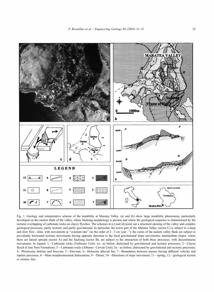
Fig. 1. Geology and interpretative scheme of the instability at Maratea Valley. (a) and (b) show large instability phenomena, particularly

developed on the eastern flank of the valley, where Sackung morphology is present and where the geological sequence is characterised by the

tectonic overlapping of carbonate rocks on clayey flysches. The schemes in (c) and (d) point out a structural opening of the valley and complex

geological processes, partly tectonic and partly gravitational. In particular, the lower part of the Maratea Valley (sector C) is subject to a deep

and slow flow–slide, with movements at ‘‘constant rate’’ (in the order of 2–3 cm year� 1); the crests of the eastern valley flank are subject to

prevalently horizontal tectonic movements having opposite direction to the local gravitational slope movements; intermediate slopes, where

there are lateral spreads (sector A) and the Sackung (sector B), are subject to the interaction of both these processes, with discontinuous

movements. In legend: 1—Carbonate rocks (Verbicaro Unit); 1a—as before, dislocated by gravitational and tectonic processes; 2—Clayey

flysch (Crete Nere Formation); 3—Carbonate rocks (Alburno–Cervati Unit); 3a—as before, dislocated by gravitational and tectonic processes;

4—Pleistocene detritus and breccias; 5—Eluvium; 6—Holocene alluvial fan; 7—Boundaries between masses having different velocity and

rupture processes; 8—Main morphostructural dislocations; 9—Thrust; 10—Directions of slope movement; 11—spring; 12—geological section

or seismic line.

P. Berardino et al. / Engineering Geology 68 (2003) 31–51 33

2. Description of the study area and available data

2.1. Geological and morphostructural setting

The Maratea Valley (Basilicata) is a tectonically

active area, affected by large complex gravitational

phenomena and impressive Sackung-type morpholo-

gies (Fig. 1a and b). The asymmetric valley has a

triangular shape, which could be divided into sectors

marked by different stratigraphy (Fig. 1c and d):

Sector A—a large area of the valley (Piano Campo)

formed by dislocated units of the Mesozoic calcare-

ous–dolomitic formations (belonging to ‘‘Bulgheria–

Verbicaro’’ tectonic unit), covered by alluvial fan, and

fragmented in aligned contiguous steps to the valley

border; Sector B—south-eastern flank of the valley

including the relief is built by the same carbonate

formations, but without detrital covers; it is affected

by impressive crest sagging and trenches, interpreted

as Sackung-type phenomena; Sector C—the remain-

ing part of the valley with outcrops of clayey for-

mations and shallow detrital covers, characterised by

landslide morphology and divided in minor sectors,

following the main structural dislocation (Fig. 1d;

Rizzo, 1997). Several springs are present along the

western border of Sectors A and B, prevalently along

the contact with the Sector C.

The complex morphostructural setting of the area

has been influenced by Pleistocene extensional tecton-

ics. Structural dislocations probably characterised by a

main transcurrent component have first allowed the

superimposition of the Bulgheria–Verbicaro unit on

the ‘‘Crete Nere’’ formation and now are facilitating the

opening of the valley (Fig. 1c and e). The ‘‘Crete Nere’’

argillitic flysch, assuming a plastic behaviour due to

high water content, is in the presence of tectonic

stresses and constitutes a ‘‘lubricant’’ for deep gravita-

tional movements (Fig. 1e).

A relation between active tectonic and slope move-

ments was hypothesised by Rizzo (1997) on the basis

of bathymetric and high-resolution seismic lines real-

ised on the sea-floor of the Maratea Valley: upper

Pleistocene–Holocene morphological, structural and

depositional setting shows in front of the valley a

structure marked along its western flank by a marine

canyon (Colantoni et al., 1997).

2.2. Previous investigation and GPS monitoring

The data on ground surface movements in the

investigated area were collected through long-term

annual monitoring, which began in 1983 (Fig. 2).

The movements were monitored through distance

variation between benchmarks and control stations

by the use of an electronic distance-meter (EDM); in

1987 and 1996, this network was updated. Based on

these data and morphostructures, a first schematic

mapping and modelling of slope instability was pro-

posed in 1996 (Rizzo, 1997).

Other data on slope movements (Figs. 2 and 3)

were collected through short-term or continuous

monitoring over different single sites within the

valley by the use of electrical extensometers and

crack gauges (Guerricchio et al., 1988) and by

inclinometric soundings (Rizzo, 1997; Rizzo and

Limongi, 1997).

Furthermore, between 1997 and 1999–2000–

2001, GPS data were acquired (Rizzo, 2001) on a

separated network which, nevertheless, shared a num-

ber of points with the EDM data. In June 1997, a

network of 42 benchmarks was set up; this grid was

used for differential static GPS monitoring, (Table 1).

The reference station was located outside of the

valley, on the carbonate slope west of Fiumicello, that

is not subject to gravitational instability (Fig. 2). In the

first campaign, two Trimble 4000SSi receivers equip-

ped with M L1/L2 ground plain antenna were

employed. The campaigns of November 1999 and

March 2000 used compensation mode and similar

equipment. GPS measurement information are col-

lected in Tables 1 and 2. The obtained results are

shown in Table 3. A new GPS network, located

outside the landslide area (on the relief constituting

the EDM monitoring reference system) was set up in

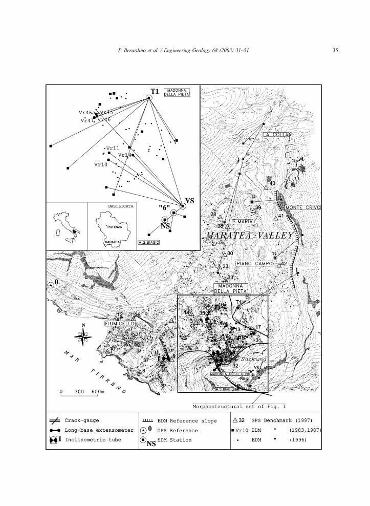
Fig. 2. Global Positioning System (GPS) and Electronic Distance Meter (EDM) monitoring networks used to measure the surface movements

(beginning 1983). The GPS measurements refer to the reference station (station 0), the stable slopes of the western flank of the valley, whereas

the EDM measurements refer to reliefs not affected by slope the gravitational processes (reference slope of Monte Crivo and Monte S. Biagio)

of the eastern flank of the valley. The figure also shows the location of instrumentation used for the measurement of deformations, both at

surface (by crack-gauges), and in depth (by inclinometric soundings); the results are shown in Fig. 3.


Fig. 3. Movements monitored in the flow–slide area of Fig. 1c, by various measurement systems and with various time intervals. The data show

a continuous gravitational process, tending to ‘‘constant rate’’, apparently little influenced by the pluviometric conditions. (a) Displacements of

benchmarks labelled Vr in Fig. 2, obtained by using an Electronic Distance Meter (EDM) from the ‘‘Madonna degli Ulivi’’ (Vs) Station (yearly

monitoring, beginning 1983). (b), (c) and (d): movements of inclinometric tubes (respectively, for tubes 1, 2 and 3 in Fig. 2), calculated at the

head (quadratic shape) and on the sliding plane (triangles) with respect to the bottom. (e) Fissure opening in a building in the old town centre,

continuously measured by an electrical crack-gauge. (f) Monitoring of the spreading of a carbonate block, continuously monitored by a long-

base invar-wire electrical extensometer anchored to the scarps of Monte S. Biagio. The graph below shows monthly rain trend in the period of

the various monitoring.


2000 in order to gather in the future a complete picture

of the instability processes.

2.3. Available data and state of knowledge

On the basis of these investigation, the previously

proposed scheme (Rizzo, 1997) was confirmed and

simplified as follows (Fig. 1d; Rizzo, 2001; Rizzo and

Leggeri, 2001):

The Sector C shows an almost constantly increas-

ing rate of movement and deformation, following the

gravitational directions, gathered both in surface and

in depth (Fig. 3), although the velocity is not spatially

homogeneous, and is therefore different from point to

point (Rizzo, 1997; Toni et al., 2001).

This kind of rupture could be seen as a constant

deep flow in high saturated clays, due to peculiar

hydrogeological condition (Cotecchia et al., 1990),

slightly influenced by rain and probably partially

influenced by tectonic (Rizzo, 1997). The depth of

flow masses is still not well known, and its study is in

progress; relevant shear plain was located in the first

50 m (Rizzo and Limongi, 1997).

In the Sectors A and B, the instability of the

Sackung and other fragmented carbonate formations

shows little and irregular movements, such as a spread

due to deep creep, that could be influenced by tectonic

activity (Rizzo, 2001). This question is still open and

first data on a new GPS network, located outside the

landslide area, confirms a role of tectonic movement

on the landslide instability and Sackung reactivation,

as proposed in Fig. 1c (Rizzo and Leggeri, 2001).

3. Employed DiffSAR technique

In this section, we describe the procedure that

allows to obtain the time evolution of ground dis-

placement corresponding to each pixel of the imaged

scene. First of all, SAR acquisitions of the considered

scene to be used in the study must be selected. In

order to make topographic phase suppression easier,

Table 1

Date and characteristics of the SAR and GPS acquisitions

Dates of SAR

acquisitions

Spatial

baseline B? (m)

Temporal

baseline (days)

Percentage of selected

points (coherence>0.3) (%)

13-08-1997 31-12-1997 30 140 33.11

31-12-1997 15-04-1998 15 105 46.74

13-08-1997 15-04-1998 45 245 30.34

15-04-1998 02-09-1998 110 140 30.85

02-09-1998 09-06-1999 2 280 33.17

02-09-1998 14-07-1999 6 315 35.28

09-06-1999 14-07-1999 4 35 52.46

09-06-1999 05-01-2000 6 210 32.05

14-07-1999 05-01-2000 10 175 29.53

Dates of GPS Work conditions (static differential; 2 h standing at rover station and minimum a week at reference station)

monitoringUtilised equipment Compensation

June 1997 N.2 Trimble 4000 with M Ll/L2

ground plain antennae

without

November 1999 N.2 Trimble 4000 and N.1 Trimble 4400

SSi with M L1/L2 ground plain antennae

on triangular grid

March 2000 N.3 Trimble 4400 SSi, N.1 Trimble 4000

with M L1/L2 ground plain antennae, N.1

Turborogue at reference station

on triangular grid

Instrumental

accuracy

in vertical: 1 + 0.1 cm for each km

of base length

(by Trimble) in horizontal: 0.5 + 0.1 cm for each

km of base length


Table 2

WGS coordinates relative to the March 2000 campaign (the benchmarks with blank cells were destroyed)

Results of GPS campaign conducted from 20 to 25 March 2000

WGS84 coordinates at reference station

x 4710295,991 lat (dms) N 40j 00V12,664Wy 1323003,504 elon (dms) E 15j 41V19,374Wz 4078378,756 wlon (dms) W 344j 18V40,626W

ht (m) 146,1940

Coordinate difference between reference and rover stations (RS)

RS dx (m) dy (m) dz (m) distance (m) dh (m) Azimuth (dms) forward

MAR1 � 128,425 1,998,270 � 443,033 2,050,818 34,737 107j 13V33,209855WMAR2 � 202,088 2,667,520 � 450,814 2,712,883 114,283 104j 36V56,335938WMAR3 � 179,138 2,400,660 � 437,538 2,446,773 84,359 105j 12V39,820661WMAR4 1521 2,251,247 � 664,766 2,341,759 53,387 112j 14V30,555003WMAR5 249,375 2,037,846 � 961,339 2,266,975 � 11,562 123j 18V39,051549WMAR6 55,099 1,870,242 � 685,161 1,992,558 � 12,106 116j 20V19,971580WMAR7 286,614 1,976,295 � 1,007,687 2,236,811 � 26,654 125j 18V39,499746WMAR8 474,715 1,628,924 � 1,144,631 2,046,687 � 47,984 135j 16V28,800690WMAR9

MA10 409,494 1,059,365 � 881,717 1,437,833 � 45,215 140j 45V19,400616WMA11 � 54,391 2,749,806 � 618,866 2,819,111 132,265 109j 02V02,255330WMA12 40,882 1,120,692 � 519,999 1,236,132 � 71,869 120j 04V33,245220WMA13 � 190,792 3,010,693 � 500,663 3,057,995 161,806 104j 58V08,829688WMA14 � 246,335 2,303,395 � 330,413 2,339,975 83,479 102j 22V19,185358WMA15

MA16 � 380,338 2,685,222 � 227,329 2,721,535 130,163 98j 34V44,449124WMA17 � 251,334 3,350,973 � 444,965 3,389,717 223,613 103j 07V13,421785WMA18 � 116,360 3,099,375 � 572,294 3,153,916 189,066 106j 42V29,758646WMA19

MA20 98,095 2,914,821 � 761,721 3,014,303 187,155 112j 29V27,231835WMA21 � 24,407 3,084,967 � 663,819 3,155,673 195,095 109j 04V51,239920WMA22

MA23 � 809,741 2,633,654 314,594 2,773,226 151,200 84j 06V25,088304WMA24

MA25

MA26 � 107,077 2,987,916 � 585,102 3,046,547 164,540 107j 14V02,428241WMA27 � 1,046,161 2,591,791 635,488 2,866,300 174,498 76j 10V 26,307833WMA28 � 1,241,614 2,528,654 1,003,283 2,990,363 253,765 68j 23V 22,341637WMA29

MA30 � 939,747 2,690,518 467,068 2,887,934 165,168 80j 35V03,971734WMA31 � 123,021 3,537,897 � 596,767 3,589,983 259,484 106j 09V00,470594WMA32 130,571 3,100,039 � 840,465 3,214,603 198,949 113j 11V26,980553WMA33 � 609,574 2,783,512 21,445 2,849,558 141,445 91j 48V56,234005WMA34 � 343,936 2,605,008 � 258,449 2,640,294 120,354 99j 33V27,544847WMA35 � 310,494 2,582,859 � 294,251 2,618,043 117,405 100j 37V28,396191WMA36 � 22,283 1,383,952 � 453,023 1,456,382 � 20,819 113j 12V19,814751WMA37 411,106 1,655,908 � 1,010,149 1,982,786 � 2875 131j 35V08,583167WMA38 � 1,209,599 2,659,290 855,331 3,044,144 209,353 71j 56V21,316074WMA39 � 1,397,718 3,056,743 1,143,109 3,550,211 338,198 69j 59V25,850068WMA40 � 1,615,336 3,205,725 1,491,427 3,887,202 432,674 65j 46V44,226765WMA41 � 1,355,440 3,447,166 1,092,427 3,861,732 417,668 73j 43V12,677252WMA42 � 929,371 3,618,644 448,267 3,762,879 353,431 85j 34V03,660213WMAT1 � 403,001 3,063,325 � 144,765 3,093,109 245,009 97j 20V26,843961W


we choose acquisitions whose orbits are enclosed

within a cylinder whose diameter is about 100 m.

All SAR images are then co-registered, so that homol-

ogous pixels in all different images correspond to the

same ground point; subsequently, interferograms are

generated by taking pairs of images. From each

interferogram, a displacement map is obtained. Then,

displacement maps are properly combined to obtain a

complete analysis of time evolution of ground dis-

placements.

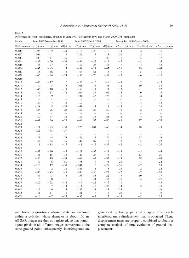
Table 3

Differences in WGS coordinates, obtained in June 1997, November 1999 and March 2000 GPS campaigns

Bench June 1997/November 1999 June 1997/March 2000 November 1999/March 2000

Mark number d1(x) mm d1( y) mm d1(z) mm d2(x) mm d2( y) mm d2(z)mm d2� d1(x) mm d2� d1( y) mm d2� d1(z) mm

MAR1 � 93 � 32 � 41 � 112 � 28 � 10 � 19 4 31

MAR2 � 106 � 1 4 � 126 4 3 � 20 5 � 1

MAR3 � 100 � 11 � 37 � 118 � 16 � 20 � 18 � 5 17

MAR4 � 87 � 20 � 31 � 94 � 22 � 17 � 7 � 2 14

MAR5 � 45 � 27 � 13 � 52 � 23 � 55 � 7 4 � 42

MAR6 � 63 � 43 17 � 84 � 24 � 47 � 21 19 � 64

MAR7 � 55 � 66 14 � 63 � 61 3 � 8 5 � 11

MAR8 � 46 � 64 � 24 � 53 � 70 � 39 � 7 � 6 � 15

MAR9 – – – – – – – – –

MA10 � 46 � 17 5 � 55 � 15 � 8 � 9 2 � 13

MA11 � 89 � 5 � 13 � 101 14 � 46 � 12 19 � 33

MA12 � 46 � 10 � 11 � 59 � 11 11 � 13 � 1 22

MA13 � 86 37 � 71 � 104 37 � 66 � 18 0 5

MA14 � 113 � 39 8 � 131 � 43 � 26 � 18 � 4 � 34

MA15 – – – – – – – – –

MA16 � 42 � 7 33 � 59 � 10 � 10 � 17 � 3 � 43

MA17 � 28 8 � 37 � 41 13 1 � 13 5 38

MA18 � 128 25 � 23 � 137 27 � 60 � 9 2 � 37

MA19 – – – – – – – – –

MA20 � 39 37 � 34 � 37 33 � 25 2 � 4 9

MA21 � 61 66 � 21 � 69 83 � 80 � 8 17 � 59

MA22 – – – – – – – – –

MA23 � 111 � 83 � 51 � 125 � 101 � 60 � 14 � 18 � 9

MA24 � 122 � 98 � 39 – – – – – –

MA25 – – – – – – – – –

MA26 � 75 44 � 73 � 76 17 � 79 � 1 � 27 � 6

MA27 � 32 � 84 � 39 � 42 � 89 � 17 � 10 � 5 22

MA28 1 � 13 � 15 � 1 � 15 � 35 � 2 � 2 � 20

MA29 – – – – – – – – –

MA30 � 93 � 90 � 7 � 111 � 95 � 11 � 18 � 5 � 4

MA31 � 31 15 � 31 � 42 28 � 5 � 11 13 26

MA32 � 56 19 � 34 � 69 47 � 97 � 13 28 � 63

MA33 � 47 � 6 � 50 � 75 � 7 � 74 � 28 � 1 � 24

MA34 � 110 17 � 51 � 141 10 � 28 � 31 � 7 23

MA35 � 110 2 � 32 � 146 4 � 8 � 36 2 24

MA36 � 86 � 43 � 7 � 88 � 50 � 27 � 2 � 7 � 20

MA37 � 46 � 43 � 5 � 53 � 53 � 22 � 7 � 10 � 17

MA38 16 � 38 � 6 8 � 34 � 33 � 8 4 � 27

MA39 � 20 � 22 � 14 � 9 � 21 � 17 11 1 � 3

MA40 0 � 7 � 14 � 14 � 5 � 22 � 14 2 � 8

MA41 � 9 � 9 3 � 32 � 8 � 3 � 23 1 � 6

MA42 � 11 � 11 12 � 31 � 8 3 � 20 3 � 9

MAT1 � 16 � 7 � 23 � 35 � 9 12 � 19 � 2 35


3.1. Generating a displacement map

In this subsection, we describe the procedure to

obtain a displacement map from an interferometric

pair. First of all, the topographic phase term must be

suppressed. In this study, we use a DEM of the area

under analysis, provided by the Italian ‘‘Istituto Geo-

grafico Militare’’ (IGM), and orbit data provided by

European Space Agency (ESA) along with SAR data.

The DEM pixel size is 20� 20 m, its vertical accuracy

is about 7–10 m and is topography dependent. After

the topographic phase term suppression, we obtain the

‘‘differential interferogram’’.

At this point, unwrapping the interferometric phase

(i.e. obtaining the correct phase from its restriction to

the interval �k,k) is a necessary step to measure

without ambiguity ground deformation. Use of tempo-

ral baselines of the order of several months causes

considerable decorrelation noise in some areas (partic-

ularly, in vegetated areas). Even when only some of the

data are corrupted, it may be impossible to unwrap the

good-quality phase in the remaining points. To over-

come this problem, the phase unwrapping operation

should be performed only on the subset of ‘‘good’’ data,

selected according to a given criterion. For instance,

this criterion can be based on the correlation coefficient

(or coherence) map (Franceschetti and Lanari, 1999) of

the interferometric pair. In general, however, the

selected data will no longer be distributed on a regular

rectangular grid, and it will not be possible to use

traditional phase unwrapping techniques. A new gen-

eralized technique, presented in Costantini and Rosen

(1999) is able to deal with sparse data, i.e. data on an

irregular grid, and can be therefore used in these cases.

Accordingly, in this method, phase unwrapping is

preceded by the selection of ‘‘good’’ points from the

differential interferogram. We select the points of the

interferograms for which the measured correlation

coefficient is greater than a prescribed threshold.

Choice of the threshold and of the size of the window

used to calculate the correlation coefficient (from the

single look complex image pair) is a delicate matter: we

verified that, for ERS data, a 3� 15 pixel window size

(corresponding to a final resolution cell of about

60� 60m) and a correlation coefficient threshold equal

to 0.3 seem to be a good choice. In fact, these values

provide a good compromise between phase ‘‘quality’’

(i.e. phase noise level) and number of selected points.

After the pixel selection, we obtain a finite set S of

irregularly distributed points in the plane. This set

represents the points for which reliable wrapped phase

data are available. The phase unwrapping algorithm

described in Costantini and Rosen (1999) and Cos-

tantini et al. (2000a) is then applied to this set of

points.

Once phase unwrapping has been performed, phase

values are converted to displacement values by multi-

plying by k/4p. The measured displacements are the

projections of actual displacements along the SAR

line of sight. The unwrapped phase values are known

up to an additive constant, different for each inter-

ferometric pair. To resolve this indetermination, it is

assumed that a given point (or, more conveniently, a

given area) in the scene is motionless. If this reference

point is not actually still, all obtained displacements

are relative to the reference point.

After determination of the phase-additive constant,

displacement values for all the irregularly distributed

points of S are available. A displacement map over the

regular original grid can be finally obtained by per-

forming a simple interpolation.

3.2. Evaluating the time evolution of ground displace-

ment

In this subsection, we describe the procedure used

to obtain the displacement time evolution for all the

points of the considered scene.

Displacement maps relative to different time inter-

vals can be combined to obtain the displacement as a

function of time. This is achieved by solving, for each

point P of the scene, the following linear system of

equations:

sðtj;PÞ � sðti;PÞ ¼ smeasðti; tj;PÞ ; i; j ¼ 1; . . . ; n ;

ð1Þ

where ti is the time of the ith acquisition, n is the total

number of acquisitions, smeas (ti, ti; P) is the displace-

ment measured over the map obtained from the pair of

SAR images acquired at times ti and tj and s(ti; P) is

the (unknown) displacement that occurred in the time

interval between the first and the ith acquisition. Once

the system (1) has been solved with respect to the

unknowns s(ti; P), the displacement values corre-


Fig. 4. Map of coherence loss (above) and of vegetation intensity (below). The pixels having a coherence higher than 0.65 are coloured and

show the obtained displacements.


sponding to the SAR acquisition times ti (i = 1,. . .,n)are available for each point of the scene.

After combining displacement maps, an atmos-

pheric artifact occurring in correspondence to a given

acquisition only affects the displacement value corre-

sponding to the time of the considered acquisition and

does not apply to other displacement values (although

it affects all the displacement maps corresponding to

pairs including the considered acquisition). The same

property holds for effects of inaccuracies in the topo-

graphic phase term subtraction due to errors in the

orbit data of a given acquisition. Hence, measured

displacement at each acquisition time can be modeled

as the sum of the true displacement value, atmos-

pheric noise and topographic noise. Therefore, it is

reasonable to fit measured displacements at different

times to a proper function of time. For the case

considered in this paper, a constant rate displacement

can be assumed (e.g. Fig. 3).

4. Results and discussion

4.1. SAR results and their interpretation

The method described in Section 3 has been used

to analyse instability in the Maratea Valley. In partic-

ular, we have considered seven ERS-2 descending

orbit SAR acquisitions covering a time interval span-

ning from August 1997 to January 2000. Due to the

dense vegetation cover (Fig. 4), a very low correlation

is obtained for pairs with high temporal spacing, so

that nine interferograms have been generated from

these acquisitions (some pairs were too decorrelated to

be used). Dates of employed SAR acquisitions and

interferograms are reported in Table 1, along with

percentages of selected points over each interfero-

gram, i.e. point where coherence is larger than 0.3.

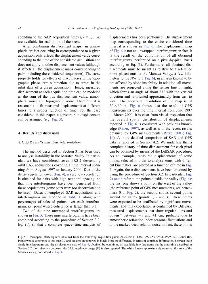
Two of the nine unwrapped interferograms are

shown in Fig. 5. These nine interferograms have been

combined according to the procedure of Section 3.2,

Eq. (1), so that a complete space–time analysis of

displacements has been performed. The displacement

map corresponding to the entire considered time

interval is shown in Fig. 6. The displacement map

of Fig. 6 is not an unwrapped interferogram; in fact, it

is the result of the combination of all obtained

interferograms, performed on a pixel-by-pixel basis

according to Eq. (1). Furthermore, all obtained dis-

placements must be meant as relative to a reference

point placed outside the Maratea Valley, a few kilo-

meters to the NW (c.f. Fig. 6), in an area known to be

not affected by slope instability. In addition, all move-

ments are projected along the sensor line of sight,

which forms an angle of about 23j with the vertical

direction and is oriented approximately from east to

west. The horizontal resolution of the map is of

60� 60 m. Fig. 6 shows also the result of GPS

measurements over the time interval from June 1997

to March 2000. It is clear from visual inspection that

the overall spatial distribution of displacements

reported in Fig. 6 is consistent with previous knowl-

edge (Rizzo, 1997), as well as with the recent results

obtained by GPS measurements (Rizzo, 2001; Fig.

1d). A more detailed comparison of SAR and GPS

data is reported in Section 4.2. We underline that a

complete history of time displacement for each pixel

can be obtained by means of the DiffSAR procedure.

As an example, measured displacements of some

points, selected in order to analyse zones with differ-

ent kinematics, are plotted as a function of time in Fig.

7. Again, these displacements have been obtained by

using the procedure of Section 3.2. In particular, Fig.

7a and b refer to the points outside the valley (Fig. 6):

the first one shows a point on the west of the valley

(the reference point of GPS measurements, see bench-

mark 0 in Fig. 2); the second shows several points

around the valley (points 1, 2 and 3). These points

were expected to be unaffected by significant move-

ments, and this expectation is confirmed by DiffSAR

measured displacements that show regular ‘‘ups and

downs’’ between �1 and +1 cm, probably due to

atmospheric refraction index seasonal fluctuations and

to the marked decorrelation noise: in fact, these points

Fig. 5. Unwrapped interferograms obtained from the following acquisition pairs: 09-06-1999 14-07-1999 (A); 09-06-1999 05-01-2000 (B).

Points whose coherence is less than 0.3 and sea area are reported in black. Note the difference, in terms of contained information, between these

single interferograms and the displacement map of Fig. 6, obtained by combining all available interferograms via the algorithm described in

Section 3.2. For reference purposes, the SAR amplitude image (C) is also reported. The white frames approximately represent the area of the

Maratea valley, considered in Fig. 6.


have a low correlation coefficient in all the employed

interferograms. Fig. 7c and d are referred to other

points placed within the valley and showing different

amount of displacements: points 4, 5, 6 and 7 in Fig.

7c and points 8 and 9 in Fig. 7d, belonging to more

and less active areas, respectively. The data clearly

show a linear dependence of displacement on time, as

expected.

4.2. Comparison with GPS measurements

GPS measurements are available from an initial

network of 43 ground points (Fig. 2, Table 3) and

refer to the period from June 1997 to March 2000

(Tables 1 and 2). However, comparison between GPS

and DiffSAR data requires some attention because of

the following issues.

First of all, the GPS reference point has turned out

to be a low-coherence point on the SAR interfero-

grams, so that we had to choose a different reference

point for DiffSAR measurements (Fig. 6). In making

this choice, we verified that the two reference points

of the two measurement systems do not significantly

move with respect each other and as regard the line of

sight direction. As a matter of fact, as shown in Fig.

7a, DiffSAR measurements over the GPS reference

point only show small fluctuations around zero that

may include both actual small movements and decor-

relation noise.

Another issue to be faced is that GPS and DiffSAR

measurements refer to different time intervals. How-

ever, considering the linearity of displacements with

time (Fig. 3), for comparison purposes, the DiffSAR

measurements were corrected in order to refer to the

same time interval as the GPS ones.

The GPS measurements are also affected by errors

(Gili et al., 2000) that can be of the same order or even

higher than DiffSAR ones. As a matter of fact, GPS

precision in horizontal plane could be of about 0.8 cm,

but could be less than 1.3 cm in the vertical direction

(data obtained for our work condition on the base of

the farmer indication). Consider also that vertical

displacements are measured by taking the difference

between three GPS campaigns, and that different (or

no) compensations have been used in the campaigns

(see Tables 1 and 3, Fig. 8). In order to quantify this,

we compared GPS measurements performed in

November 1999 with those performed on March

2000. The differences between the vertical compo-

nents of the two measurements (Table 3), depurated of

the small actual movements predicted over 4 months

(this prediction is based on the constant displacement

rates measured by the June 1997–March 2000 GPS

campaign at every benchmark) are plotted in Fig. 9 for

the GPS ground points. The data show fluctuations in

the order of 2–2.5 cm, having a maximum of 6 cm. In

order to obtain values homogeneous with the DiffSAR

ones, we also projected GPS errors onto the SAR line

of sight. The standard deviation of these projected

errors turns out to be 2.3 cm, which can be considered

as the GPS error (obviously higher than the instru-

mental precision, as consequence of previous assump-

tion and elaboration) along the SAR line of sight.

Unfortunately only very few of the GPS ground

points have a high coherence value on all the inter-

ferograms. More exactly, only for 3 out of 42 GPS

ground points, the average value of coherence is

greater than 0.65. Corresponding results are reported

in Table 4 (points 4, 13 and 17). The difference

between GPS and DiffSAR measurements in these

cases is always smaller than GPS error, thus confirm-

ing the effectiveness of our technique in high coher-

ence areas. With regard to measurements on the other

(i.e. low coherence) points, the difference between

GPS and DiffSAR measurements (see Table 4) has a

mean value equal to � 2.3 cm (DiffSAR underesti-

mates the movements) and a standard deviation equal

to 3.3 cm. These discrepancies can be explained by

considering that in these low-coherence points the

DiffSAR measurements are obtained by interpolating

results obtained in surrounding high-coherence points,

so that they can be considered as average displace-

ment over a rather wide area, whereas GPS measure-

ments are strictly referred to each single ground point.

In addition, as already pointed out, SAR and GPS

measurements have been reported to the same time

Fig. 6. Above: DiffSAR displacement map relative to the period from August 1997 to January 2000, and GPS data acquired in almost the same

time interval (June 1997–March 2000). GPS vectors shown by arrows lie in the horizontal plane, whereas SAR displacements are as projected

along the line of sight (descending orbit, being about 23j from vertical and 104j from the direction north). Below: map showing locations of

DiffSAR reference point and of SAR points (pixels) and GPS measurement points selected for temporal displacement analysis (Fig. 7).


interval by relying on the constant rate assumption,

and hence, this operation may be slightly affected by

limitations of the assumption. The above results

suggest that DiffSAR accuracy is higher than the

GPS one if the coherence (averaged over all the

interferograms) is greater than 0.65, i.e. in the areas

highlighted in Fig. 4. Such data can be used to

‘‘complement’’ the GPS network. Measurements per-

formed outside these areas must be understood as

spatially averaged measurements, not useful to

retrieve the exact displacement of a particular consid-

ered ground point, but useful to understand the overall

kinematics of the slope instability phenomenon.

4.3. Geological model based on integration of SAR

and GPS data

According to the results of the previous subsec-

tion, integration of GPS and DiffSAR data can lead

to a more complete analysis. Due to the SAR

acquisition geometry, DiffSAR mainly measures the

vertical component of the movement that is not

always accurately estimated by the GPS technique.

Improvement in the understanding of the vertical

component allowed us to obtain a detailed schemati-

sation of the kinematics of the Maratea Valley,

reported in Fig. 10. The area under survey has been

Fig. 7. Displacement versus time for points 1–9 reported in Fig. 6 and for GPS reference pixel (coincident to Station 0 in Fig. 2). (a) The GPS

reference point. (b) A set of stable points outside the valley (point 1: asterisks; point 2: diamonds; point 3: triangles). (c) A set of points within

the valley in the area showing intense vertical displacements (a large strip going from the northern border of the Sackung to Fiumicello on the

coast (point 4: asterisks; point 5: diamonds; point 6:triangles; point 7: squares). (d) Two points within the valley (point 8: asterisks; point 9:

triangles) in the south-eastern corner showing minor vertical displacements.


Fig. 8. Configuration of the GPS compensation networks used in the June 1997, November 1999 and March 2000 campaigns.

Fig. 9. Difference between the vertical component of GPS measurements of November 1999 and March 2000; both with respect to that of June

1997. These differences have been depurated of the small movements predicted over 4 months, supposing that the velocity monitored with GPS

techniques for every single point proceeds ‘‘at constant rate’’. In fact, this procedure, necessary to make the data coherent from the point of view

of the time interval, is not influential since the aforementioned campaigns were almost coeval. It should be noted how the differences in quota

obtained for the various benchmarks are slightly higher than the accuracy known for these measurement systems.


Table 4

Comparison of GPS and DiffSAR measurements

GPS

benchmark

number

GPS

displacement

(mm)

DiffSAR

displacement

(mm)

Zone in

the model

(Fig. 10)

Coherence Linearity GPS-SAR

difference

(mm)

1 � 52 � 54 2 0.3 1 2

2 � 49 � 63 2 0.6 0.9 14

3 � 65 � 63 2 0.5 1 � 2

4 � 52 � 54 3 0.7 0.9 2

5 � 69 � 22 2 0.2 0.7 � 47

6 � 75 � 24 3 0.6 0.8 � 51

7 � 18 � 15 2 0.2 0.5 � 3

8 � 51 � 8 3 0.3 0.4 � 43

9 no � 25 3 0.6 0.8

10 � 28 � 6 3 0.2 0 � 22

11 � 84 � 56 2 0.2 0.9 � 28

12 � 13 � 36 2 0.2 0.8 23

13 � 105 � 83 2 0.7 1 � 22

14 � 73 � 52 2 0.3 0.9 � 21

15 no � 47 2 0.3 0.9

16 � 32 � 65 2 0.3 1 33

17 � 17 � 38 2 0.7 0.8 21

18 � 112 � 46 2 0.6 0.9 � 66

19 no � 14 2 0.4 0.1

20 � 41 � 15 2 0.4 0 � 26

21 � 107 � 27 2 0.6 0.6 � 80

22 no � 58 2 0.3 0.9

23 � 97 � 51 2 0.3 1 � 46

24 no � 69 2 0.3 1

25 no � 69 2 0.3 1

26 � 104 � 56 2 0.6 0.9 � 48

27 � 24 � 75 2 0.2 1 51

28 � 31 � 18 2 0.3 0.3 � 13

29 no 2 2 0.2 0

30 � 47 � 41 2 0.3 1 � 6

31 � 24 � 18 2 0.2 0.6 � 6

32 � 120 � 33 2 0.1 0.7 � 87

33 � 97 � 13 2 0.2 0.8 � 84

34 � 83 � 68 2 0.4 0.9 � 15

35 � 66 � 61 2 0.5 0.9 � 5

36 � 56 � 38 2 0.2 0.9 � 18

37 � 37 � 15 3 0.2 0.7 � 22

38 � 24 � 56 1 0.2 0.7 32

39 � 17 � 9 1 0.2 0 � 8

40 � 25 � 25 1 0.4 0.6 0

41 � 15 � 21 1 0.2 0.7 6

42 � 9 � 26 1 0.3 0.5 17

Displacements are both relative to the period from June 1997 to March 2000 and are projected along the SAR line of sight. GPS error, on the

basis of the data shown in Fig. 9, is 23 mm. The obtained values show good agreement in the pixels at higher coherence.

In the other cases the differences found are due to two different acquisition systems: in part attributable to GPS errors in the vertical direction,

where the SAR data seem to be more reliable; in part to the contribution to the coherence of the various objects in movement present in the SAR

pixels, with respect to the fixed and limited position of the individual GPS benchmark; in part to the difference between SAR and GPS reference

points.


divided into four kinematics typologies: (1) area

subject to very low and irregular movements (about

0.5 cm year� 1); (2) area subject to intense move-

ments, both vertical and horizontal (about 2–4 cm

year� 1); (3) area subject to prevalently horizontal

movements (of similar amount); (4) area external to

the valley and not subject to relevant vertical dis-

placements (and still being monitored by GPS to

control horizontal displacements). In addition, in

Fig. 10, the stable reference area placed on the right

flank of the valley is shown as region 5.

Note that the zone with a marked vertical compo-

nent is wider than previously believed (Toni et al.,

2001): it includes not only the area between Maratea

Village and S. Maria, but also a larger strip that goes

from the northern margin of the Sackung to Fiumi-

cello on the coast (Figs. 1, 2 and 6); where there is the

submarine canyon interpreted in previous work as

Fig. 10. Modelling of the instability at Maratea. The differences from the Fig. 1 scheme are the result of a re-elaboration based on the DiffSAR

data only. Legend: 1—Deep creep zone, characterized by low and irregular gravitational movements (about 0.5 cm year� 1 or less), as a

consequence of opposing tectonic (widening valley) and gravitational movements (creep); 2—Clayey flow: characterised by intense

gravitational movements (both in vertical and horizontal direction of about 2–4 cm year� 1); 3—Flow, as above, but characterised by only

intense horizontal movements; 4—Areas not subjected to gravitational movements, but probably subject to intense tectonic movements; 5—

Stable slopes and utilised as GPS reference. Area 1 near the lower margin of the picture shows the Sackung.


consequence of tectonic activity (Rizzo, 1997). In

addition, the DiffSAR measurements seem to confirm

the presence of a recently detected movements on the

carbonate slope of the valley, constituting the north-

western border of the flow along the valley, once

assumed to be without movement.

5. Summary and conclusions

In this paper, the use of the DiffSAR technique to

improve our knowledge of the slope instability of a

well-investigated area (the Maratea Valley) affected

by continuous slow movements has been explored.

Advantages of the proposed interferometric proce-

dure are those common to other implementations of

DiffSAR technique, i.e. global coverage and spatial

and (with some limitations) temporal continuity of

displacement measurements. An additional important

advantage of our procedure is that it allows to

mitigate the effects of temporal decorrelation and

atmospheric artifacts. In fact, the study area is

strongly vegetated, so that interferometric coherence

is low in a high percentage of scene points. In spite

of that, the obtained DiffSAR results are consistent

with previous knowledge of the considered phenom-

enon.

Comparison of DiffSAR and GPS vertical dis-

placements has shown that, for high-coherence points,

precision of DiffSAR is higher. Accuracy in low-

coherence areas is less satisfactory, and measurements

in these areas must be understood as spatially aver-

aged measurements; they do not allow to retrieve the

exact displacement of single ground points, but are

useful to understand the overall kinematics of the

instability phenomenon. Hence, obtained results allow

to carry out a complete analysis of the whole valley

and its surroundings.

In particular, we can conclude that:

(a) integration of the GPS and DiffSAR data has

allowed to obtain a new and more detailed picture

of the kinematics within the Maratea Valley; the

valley has been subdivided into four zones with

different ground movement characteristics;

(b) DiffSAR temporal analysis is coherent with the

result of other displacement monitoring networks

showing a deformation at constant rate;

(c) No DiffSAR vertical movements were detected on

the Sackung area in the monitored time interval,

proving a scarce influence of moderate quakes

(September 9, 1998 earthquakes of Castelluccio;

VI–VII MCS; 20 km far from Maratea) on its

stability.

Acknowledgements

This work has been supported by the Italian Space

Agency (ASI), within the project ‘‘Interferometria

differenziale per il controllo delle frane: uso diretto e

integrato con altre tecniche’’, by the financial help of

CNR-GNDCI line 2 (authorisation no. 2465) and POP

Basilicata measure 9.4.

References

Achache, J., Fruneau, B., Delacourt, C., 1995. Applicability of

SAR interferometry for operational monitoring of landslides.

Proceedings of the Second ERS Applications Workshop,

pp. 165–168.

Carnec, C., Massonnet, D., King, C., 1996. Two examples of the

use of SAR interferometry on displacement-fields of small spa-

tial extent. Geophysical Research Letters 23 (24), 3579–3582.

Colantoni, P., Gabbianelli, G., Rizzo, V., Piergiovanni, A., 1997.

Atti del Convegno ‘‘Grandi fenomeni gravitativi lenti nelle re-

gioni alpine ed appenniniche’’, Maratea, 28 – 30 Settembre

1995. Geografia Fisica Dinamica Quaternaria 20, 51–60.

Costantini, M., Rosen, P.A., 1999. A generalized phase unwrapping

approach for sparse data. Proceedings of the International Geo-

science and Remote Sensing Symposium, pp. 267–269.

Costantini, M., Iodice, A., Magnapane, L., Pietranera, L., 2000a.

Monitoring terrain movements by means of sparse SAR differ-

ential interferometric measurements. Proceedings of the Interna-

tional Geoscience and Remote Sensing Symposium, Honolulu,

HA, USA, pp. 3225–3227.

Costantini, M., Iodice, A., Pietranera, L., 2000b. Temporal analysis

of terrain subsidence by means of sparse SAR differential inter-

ferometric measurements. Proceedings of the EOS/SPIE Sym-

posium on Remote Sensing, Conference on SAR Image A-

nalysis, Modelling, and Techniques, Barcelona (Spain), vol. II,

pp. 12–18.

Cotecchia, V., D’Ecclesiis, G., Polemio, M., 1990. Studio geologico

ed idrogeologico dei Monti di Maratea. Geologia Applicata e

Idrogeologia XXV, 139–179.

Ferretti, A., Prati, C., Rocca, F., 2001. Permanent scatterers in SAR

interferometry. IEEE Transactions on Geoscience and Remote

Sensing 39 (1), 8–20.

Franceschetti, G., Lanari, R., 1999. Synthetic Aperture Radar Pro-

cessing. CRC, Boca Raton, FL, pp. 25–28.

Fruneau, B., Achace, J., Delacourt, C., 1996. Observation and mod-


elling of the Sant-Etienne-de Tinee landslide using SAR inter-

ferometry. Tectonophysics 265, 181–190.

Gili, J.A., Corominas, J., Rius, J., 2000. Using Global Positioning

System techniques in landslide monitoring. Engineering Geol-

ogy 55, 167–192.

Goldstein, R.M., Zebker, H.A., Werner, C.L., Rosen, P.A., Gabriel,

A., 1994. On the derivation of coseismic displacement field

using differential radar interferometry: The Landers earthquake.

Journal of Geophysical Research 99, 9618–9634.

Guerricchio, A., Melidoro, G., Rizzo, V., 1986. Prime osservazioni

strumentali delle deformazioni dei pendii e delle manifestazioni

profonde nella valle di Maratea (Basilicata, Italia). Geologia

Tecnica 4/86, 35–48.

Guerricchio, A., Melidoro, G., Rizzo, V., 1988. Instrumental obser-

vation of the slope deformation and deep phenomena in Maratea

Valley (Italy). Proc. Fifth ISL, Lausanne, 10–15 July. Bonnaud

edit., Balkema, Netherlands, pp. 415–422.

Massonnet, D., Rossi, M., Carmona, C., Adragna, F., Peltzer, G.,

Feigl, K., Rabaute, T., 1993. The displacement field of the

Landers earthquake mapped by radar interferometry. Nature

364, 138–142.

Massonnet, D., Briole, P., Arnaud, A., 1995. New insights on

Mount Etna from 18 months of radar interferometric monitor-

ing. Nature 375, 567–570.

Rizzo, V., 1997. Processi morfodinamici e movimenti del suolo nela

Valle di Maratea (Basilicata). Atti del Convegno ‘‘Grandi feno-

meni gravitativi lenti nelle regioni alpine ed appenniniche’’,

Maratea, 28–30 Settembre 1995. Geografia Fisica e Dinamica

Quaternaria 20, 119–136.

Rizzo, V., 2001. New data on slope movements in the Maratea

Valley (Potenza, Basilicata). Abstracts of EGS General Assem-

bly, March, Nice, 276.

Rizzo, V., Leggeri, M., 2001. Seismic activity and recent acceler-

ation of gravitational processes on the Creep area at left flanc of

Maratea Valley (Potenza, Basilicata). Abstracts of EGS General

Assembly, March, Nice, 277.

Rizzo, V., Limongi, P., 1997. Risultati inclinometrici ed indagini

geologico-stratigrafiche nel Centro Storico di Maratea (Lucania,

Italia). Geografia Fisica e Dinamica Quaternaria 20, 137–144.

Rizzo, V., Tesauro, M., 2000. SAR interferometry and field data of

Randazzo landslide (Eastern Sicily, Italy). Physics and Chem-

istry of the Earth 25 (9), 771–780.

Rott, H., Scheuchl, B., Siegel, A., Grasemann, B., 1999. Mon-

itoring very slow slope motion by means of SAR interferom-

etry: a case study from a mass waste above a reservoir in the

Otzal Alps, Austria. Geophysical Research Letters 26 (11),

1629–1632.

Toni, G., Rizzo, V., Rijillo, R., 2001. Monitoring and modelling of

collapse structures as consequence of different flow speeds

(Maratea Valley, Basilicata region, Italy). Abstracts presented

to EGS General Assembly, March, Nice, 275.


Use of differential SAR interferometry in monitoring and modelling large slope instability at...

Documents

Transcript of Use of differential SAR interferometry in monitoring and modelling large slope instability at...