SAR Image Analysis and Target Detection Utilizing

Polarimetric Information

DISSERTATION

submitted in partial satisfaction of the requirements

for the degree of

DOCTOR OF PHILOSOPHY

National Defense Academy

Graduate School of Science and Engineering

Electronics and Information Engineering

Concentration in Computer, Intelligent and Media Systems

Mitsunobu Sugimoto

March 2013

Table of Contents

Page

Table of Contents ii

List of Figures iv

List of Tables viii

List of Symbols and Abbreviations ix

Acknowledgments xiv

Abstract of the Dissertation xvi

1 Introduction 11.1 Synthetic Aperture Radar . . . . . . . . . . . . . . . . . . . . . . . . 11.2 Selected Spaceborne and Airborne SAR . . . . . . . . . . . . . . . . . 41.3 Other Recent Trends in SAR . . . . . . . . . . . . . . . . . . . . . . . 81.4 Purpose of This Study . . . . . . . . . . . . . . . . . . . . . . . . . . 101.5 Outline of the Thesis . . . . . . . . . . . . . . . . . . . . . . . . . . . 11

2 SAR Fundamentals 132.1 SAR System Parameters . . . . . . . . . . . . . . . . . . . . . . . . . 14

2.1.1 Geometry of SAR System . . . . . . . . . . . . . . . . . . . . 142.1.2 Signal Parameters . . . . . . . . . . . . . . . . . . . . . . . . . 15

2.2 Image Formation in Range Direction . . . . . . . . . . . . . . . . . . 162.2.1 Image Formation with Rectangular Pulses . . . . . . . . . . . 172.2.2 Image Formation with the Pulse Compression Technique . . . 18

2.3 Image Formation in Azimuth Direction . . . . . . . . . . . . . . . . . 262.3.1 Image Formation with Real Aperture Radar . . . . . . . . . . 262.3.2 Image Formation with Aperture Synthesis . . . . . . . . . . . 30

3 SAR Polarimetric Analysis 403.1 Polarization State of Electromagnetic Waves . . . . . . . . . . . . . . 413.2 Matrix Representation of PolSAR Data . . . . . . . . . . . . . . . . . 443.3 Model-based Decomposition Analysis . . . . . . . . . . . . . . . . . . 483.4 Eigenvalue Decomposition Analysis . . . . . . . . . . . . . . . . . . . 50

ii

4 4-CSPD Algorithm with Rotation of Covariance Matrix 564.1 Overview . . . . . . . . . . . . . . . . . . . . . . . . . . . . . . . . . . 574.2 Rotation of Covariance Matrix . . . . . . . . . . . . . . . . . . . . . . 594.3 4-CSPD Algorithm Using Rotated Covariance Matrix . . . . . . . . . 624.4 Experimental Results and Discussions . . . . . . . . . . . . . . . . . . 65

5 Comparison between Eigenvalue Analyses of Different Polarization 715.1 Introduction . . . . . . . . . . . . . . . . . . . . . . . . . . . . . . . . 725.2 Methodology . . . . . . . . . . . . . . . . . . . . . . . . . . . . . . . 735.3 Polarimetric SAR Data . . . . . . . . . . . . . . . . . . . . . . . . . . 755.4 Experimental Results and Discussions . . . . . . . . . . . . . . . . . . 75

6 Marine Target Detection Using the Model-Based Decomposition 826.1 Introduction . . . . . . . . . . . . . . . . . . . . . . . . . . . . . . . . 836.2 Methodology . . . . . . . . . . . . . . . . . . . . . . . . . . . . . . . 846.3 PolSAR Data and Ground Truth . . . . . . . . . . . . . . . . . . . . 866.4 Experimental results and Discussions . . . . . . . . . . . . . . . . . . 89

7 Comprehensive Comparison of Different Polarimetric Methods 967.1 Introduction . . . . . . . . . . . . . . . . . . . . . . . . . . . . . . . . 977.2 Interaction between Laver Cultivation Area and SAR Microwaves . . 987.3 Experimental results and Discussions . . . . . . . . . . . . . . . . . . 100

8 Conclusions 111

Bibliography 115

iii

List of Figures

Page

1.1 Illustrating the three active microwave instruments on board of SEASAT.The radar scatterometer consisting of two pairs of three rod antennaswas used to measure ocean winds, and the parabola antenna point-ing at nadir was the radar altimeter to measure ocean surface height.The SAR antenna was 10.7m in the along-track direction and 2.2m inthe cross-track direction with the off-nadir angle of 23◦. (Courtesy ofNASA/JPL) . . . . . . . . . . . . . . . . . . . . . . . . . . . . . . . . 2

1.2 Outline of the thesis . . . . . . . . . . . . . . . . . . . . . . . . . . . 12

2.1 Illustration of SAR geometry. . . . . . . . . . . . . . . . . . . . . . . 152.2 Pulses and observation window of spaceborne SAR. fp is pulse rep-

etition frequency, tp is pulse repetition time and the inverse numberof fp, and τw is the time duration of the observation window. Theobservation window is for the first transmitted pulse. . . . . . . . . . 16

2.3 Illustrating range imaging process and resolution of a conventionalradar with rectangular pulses. . . . . . . . . . . . . . . . . . . . . . . 18

2.4 Illustrating (a) the real component of the phase of a FM pulse and (b)instantaneous frequency with ωc = 0. . . . . . . . . . . . . . . . . . . 20

2.5 Change of coordinate origin in slant-range time. (a) Origin at theantenna. (b) Origin at the ground. . . . . . . . . . . . . . . . . . . . 23

2.6 Intensity point spread function in range direction. . . . . . . . . . . . 242.7 Illustrating azimuth resolution of a conventional radar. . . . . . . . . 282.8 (a) Beam pattern in azimuth direction. (b) Resolution: in the case of

sinc function beam pattern. . . . . . . . . . . . . . . . . . . . . . . . 292.9 Illustration of a geometry of a point scatterer and the platform at

different azimuth times. . . . . . . . . . . . . . . . . . . . . . . . . . 302.10 Aligned received pulses. . . . . . . . . . . . . . . . . . . . . . . . . . 322.11 Top view of the re-arranged 2-D signal. . . . . . . . . . . . . . . . . . 332.12 A received 2-D signal after the range compression. . . . . . . . . . . . 342.13 A received 2-D signal after the range migration compensation. . . . . 35

3.1 Electric field of linear polarization. . . . . . . . . . . . . . . . . . . . 413.2 Electric field of circular polarization. . . . . . . . . . . . . . . . . . . 423.3 Polarization ellipse. . . . . . . . . . . . . . . . . . . . . . . . . . . . . 43

iv

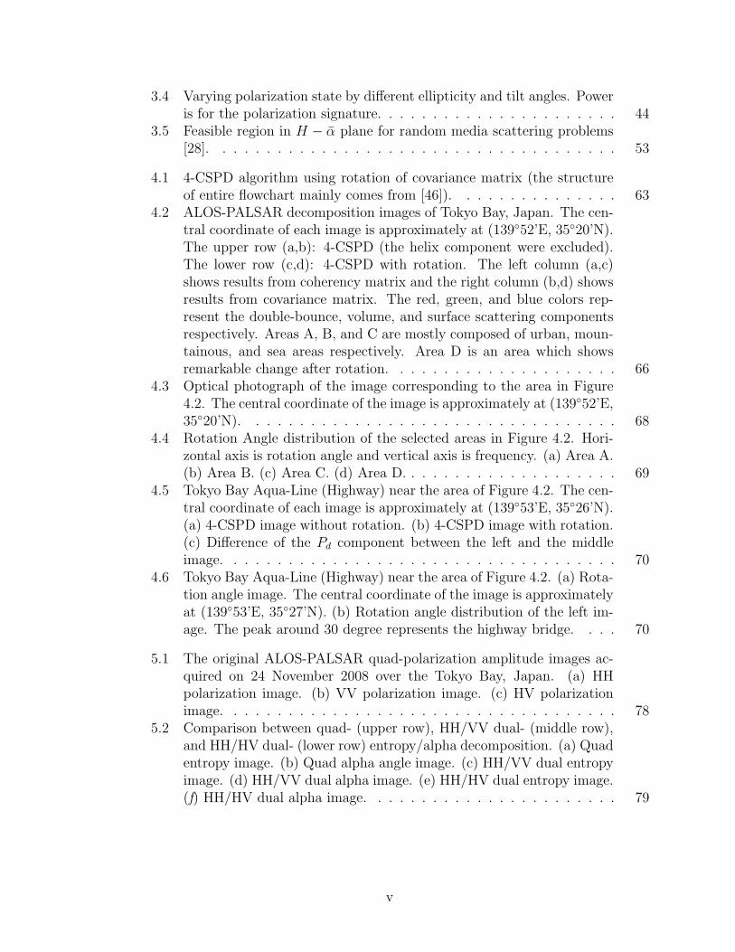
3.4 Varying polarization state by different ellipticity and tilt angles. Poweris for the polarization signature. . . . . . . . . . . . . . . . . . . . . . 44

3.5 Feasible region in H − α plane for random media scattering problems[28]. . . . . . . . . . . . . . . . . . . . . . . . . . . . . . . . . . . . . 53

4.1 4-CSPD algorithm using rotation of covariance matrix (the structureof entire flowchart mainly comes from [46]). . . . . . . . . . . . . . . 63

4.2 ALOS-PALSAR decomposition images of Tokyo Bay, Japan. The cen-tral coordinate of each image is approximately at (139◦52’E, 35◦20’N).The upper row (a,b): 4-CSPD (the helix component were excluded).The lower row (c,d): 4-CSPD with rotation. The left column (a,c)shows results from coherency matrix and the right column (b,d) showsresults from covariance matrix. The red, green, and blue colors rep-resent the double-bounce, volume, and surface scattering componentsrespectively. Areas A, B, and C are mostly composed of urban, moun-tainous, and sea areas respectively. Area D is an area which showsremarkable change after rotation. . . . . . . . . . . . . . . . . . . . . 66

4.3 Optical photograph of the image corresponding to the area in Figure4.2. The central coordinate of the image is approximately at (139◦52’E,35◦20’N). . . . . . . . . . . . . . . . . . . . . . . . . . . . . . . . . . 68

4.4 Rotation Angle distribution of the selected areas in Figure 4.2. Hori-zontal axis is rotation angle and vertical axis is frequency. (a) Area A.(b) Area B. (c) Area C. (d) Area D. . . . . . . . . . . . . . . . . . . . 69

4.5 Tokyo Bay Aqua-Line (Highway) near the area of Figure 4.2. The cen-tral coordinate of each image is approximately at (139◦53’E, 35◦26’N).(a) 4-CSPD image without rotation. (b) 4-CSPD image with rotation.(c) Difference of the Pd component between the left and the middleimage. . . . . . . . . . . . . . . . . . . . . . . . . . . . . . . . . . . . 70

4.6 Tokyo Bay Aqua-Line (Highway) near the area of Figure 4.2. (a) Rota-tion angle image. The central coordinate of the image is approximatelyat (139◦53’E, 35◦27’N). (b) Rotation angle distribution of the left im-age. The peak around 30 degree represents the highway bridge. . . . 70

5.1 The original ALOS-PALSAR quad-polarization amplitude images ac-quired on 24 November 2008 over the Tokyo Bay, Japan. (a) HHpolarization image. (b) VV polarization image. (c) HV polarizationimage. . . . . . . . . . . . . . . . . . . . . . . . . . . . . . . . . . . . 78

5.2 Comparison between quad- (upper row), HH/VV dual- (middle row),and HH/HV dual- (lower row) entropy/alpha decomposition. (a) Quadentropy image. (b) Quad alpha angle image. (c) HH/VV dual entropyimage. (d) HH/VV dual alpha image. (e) HH/HV dual entropy image.(f) HH/HV dual alpha image. . . . . . . . . . . . . . . . . . . . . . . 79

v

5.3 Enlarged images of selected areas from Figure 5.2. From left to rightcolumn, sea, vegetation, and urban areas are shown. (a)-(c) Quadentropy. (d)-(f) HH/VV dual entropy. (g)-(i) HH/HV dual entropy.(j)-(l) Quad alpha angle. (m)-(o) HH/VV dual alpha angle. (p)-(r)HH/HV dual alpha angle. . . . . . . . . . . . . . . . . . . . . . . . . 80

5.4 Entropy/alpha plots of selected areas from quad- (upper row), HH/VVdual- (middle row), and HH/HV dual- (lower row) eigenvalue analyses.From left to right column, sea, vegetation, and urban areas are shown.(a)-(c) Quad entropy/alpha plot. (d)-(f) HH/VV dual entropy/alphaplot. (g)-(i) HH/HV dual entropy/alpha plot. . . . . . . . . . . . . . 81

6.1 Scattering from ships. . . . . . . . . . . . . . . . . . . . . . . . . . . . 846.2 Flowchart of detection process. . . . . . . . . . . . . . . . . . . . . . 866.3 A Google Map image of the area around Portsmouth. The central co-

ordinate of the image is approximately at 50◦45’N, 1◦04’W. The whiterectangle at the center of the image represents the test site analyzedin this study. Imagery c⃝2012 TerraMetrics. Map data c⃝2012 Google(accessed November 6, 2012). . . . . . . . . . . . . . . . . . . . . . . 87

6.4 The ALOS-PALSAR quad-polarization amplitude images and the de-composed image. The image centre is approximately at 50◦46’N, 1◦04’Wand the image size is approximately 5 km in both azimuth and rangedirections. (a) HH image. (b) VV image. (c) HV image. (d) De-composed image of the test site (red: double-bounce scattering, green:volume scattering, blue: surface scattering). The white rectangle is anarea chosen as the homogeneous background area. . . . . . . . . . . . 88

6.5 Nautical map as reference data. c⃝Portsmouth Port 2011 (accessedNovember 5, 2012). . . . . . . . . . . . . . . . . . . . . . . . . . . . . 90

6.6 (a) TP −Ps image. (b) Statistical intensity distribution of backgroundarea marked as rectangles in (a) and candidate PDFs. . . . . . . . . . 91

6.7 (a) Optimized Pd image. (b) Statistical intensity distribution of back-ground area marked as rectangles in (a) and candidate PDFs. . . . . 91

6.8 Receiver operating characteristic (ROC) curves. . . . . . . . . . . . . 926.9 Detection result by TP − Ps (solid circles: detected targets, dashed

circles: missed targets). . . . . . . . . . . . . . . . . . . . . . . . . . . 936.10 Detection result by optimized Pd (solid circles: detected targets, dashed

circles: missed targets) . . . . . . . . . . . . . . . . . . . . . . . . . . 93

vi

6.11 Ship detection using fully polarimetric ALOS-PALSAR data aroundTokyo bay on 9 October, 2008. The image center is at approximately35◦17’N, 139◦44’E, and the image size is approximately 10 km in rangeand 7 km in azimuth directions. Solid circles: visible/detected tar-gets. Dashed circles: invisible/missed targets. Rectangles: two seaforts (top) and an island (left). (a) Decomposed image of the test siteobtained using the 4-CSPD algorithm (red: double-bounce scatter-ing, green: volume scattering, blue: surface scattering). (b) Detectionresult obtained by excluding the surface scattering component. (c)Detection result obtained using the optimized Pd . . . . . . . . . . . . 95

7.1 Photograph of a part of the Futtsu Horn test area in Tokyo Bay, Japantaken on 5th of February 2011. . . . . . . . . . . . . . . . . . . . . . 99

7.2 The ALOS-PALSAR quad-polarization amplitude images acquired on24 November 2008 over Tokyo Bay, Japan. (a) HH polarization image.(b) VV polarization image. (c) HV polarization image. . . . . . . . . 100

7.3 Comparison of image contrast between laver cultivation area and back-ground area using methods with HH and VV dual-polarization combi-nation from ALOS-PALSAR data. . . . . . . . . . . . . . . . . . . . . 104

7.4 Comparison of image contrast between laver cultivation area and back-ground area using methods with quad-polarization data from ALOS-PALSAR. . . . . . . . . . . . . . . . . . . . . . . . . . . . . . . . . . 105

7.5 TerraSAR-X amplitude images of Futtsu Horn laver cultivation areain Tokyo Bay, Japan. The data were acquired on October 20, 2011(upper row (a) and (b)) and December 26, 2008 (lower row (c) and(d)). (a)(c): HH amplitude image. (b)(d): VV amplitude image. . . . 106

7.6 Comparison of image contrast between laver cultivation area and back-ground using TerraSAR-X HH/VV dual-polarization data in 2011. Thevalues next to each caption are mean contrasts. (a) HH+VV image:0.001. (b) HH-VV image: 0.327. (c) Entropy image: 0.253. (d) Scat-tering angle image: 0.348. (e) HH/VV coherence image: 0.674. (f)Phase difference image: 0.226. . . . . . . . . . . . . . . . . . . . . . . 109

7.7 Comparison of image contrast between laver cultivation area and back-ground using TerraSAR-X HH/VV dual-polarization data in 2008. Thevalues next to each caption are mean contrasts. (a) HH+VV image:0.254. (b) HH-VV image: 0.244. (c) Entropy image: 0.465. (d) Scat-tering angle image: 0.008. (e) HH/VV coherence image: 0.031. (f)Phase difference image: 0.008. . . . . . . . . . . . . . . . . . . . . . . 110

vii

List of Tables

Page

1.1 Selected fields of SAR application examples. Note that not all appli-cations are in practical use; many applications are still at developingstages [3]. . . . . . . . . . . . . . . . . . . . . . . . . . . . . . . . . . 2

1.2 Parameters of selected spaceborne SARs. “Pol.” means the availablecombination of polarization states, “Res.” indicates the finest availablespatial resolutions in azimuth/range directions, “Weight” is in kg, and“Alt.” is the average orbit altitude in km. The parentheses next tosensor name are the number of identical satellites. . . . . . . . . . . . 5

1.3 Common frequency bands for radar systems. . . . . . . . . . . . . . . 81.4 Parameters of selected airborne SARs. “Res.” indicates the maximum

achievable spatial resolutions in azimuth/range directions. Most of thelisted airborne SARs operate in quad- (quadrature) polarization withinterferometric modes. UAV next to sensor name stands for UnmannedAerial Vehicle. . . . . . . . . . . . . . . . . . . . . . . . . . . . . . . . 9

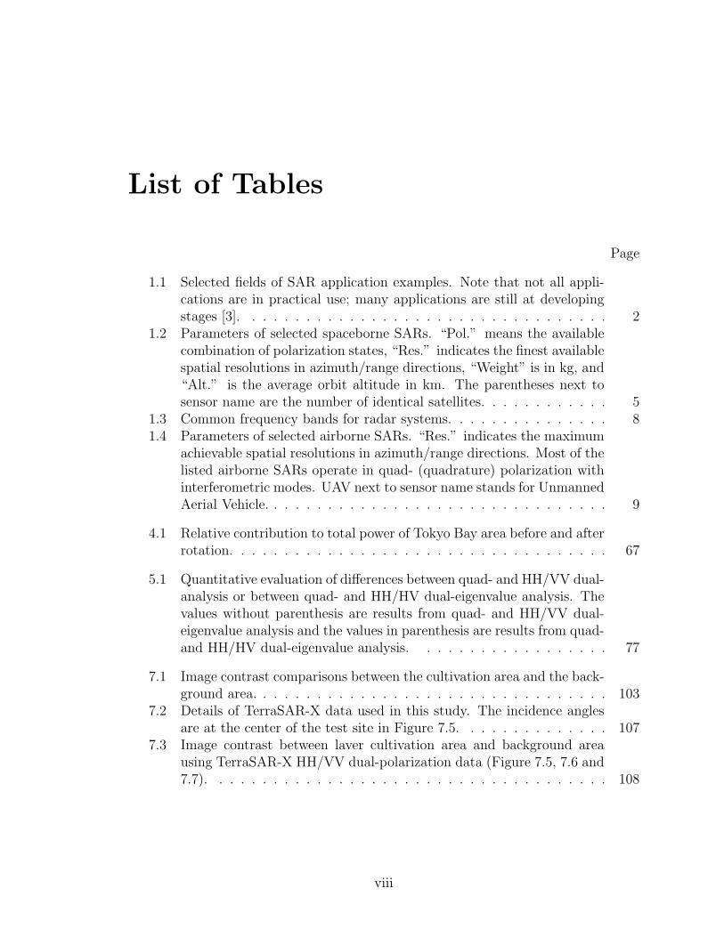
4.1 Relative contribution to total power of Tokyo Bay area before and afterrotation. . . . . . . . . . . . . . . . . . . . . . . . . . . . . . . . . . . 67

5.1 Quantitative evaluation of differences between quad- and HH/VV dual-analysis or between quad- and HH/HV dual-eigenvalue analysis. Thevalues without parenthesis are results from quad- and HH/VV dual-eigenvalue analysis and the values in parenthesis are results from quad-and HH/HV dual-eigenvalue analysis. . . . . . . . . . . . . . . . . . 77

7.1 Image contrast comparisons between the cultivation area and the back-ground area. . . . . . . . . . . . . . . . . . . . . . . . . . . . . . . . . 103

7.2 Details of TerraSAR-X data used in this study. The incidence anglesare at the center of the test site in Figure 7.5. . . . . . . . . . . . . . 107

7.3 Image contrast between laver cultivation area and background areausing TerraSAR-X HH/VV dual-polarization data (Figure 7.5, 7.6 and7.7). . . . . . . . . . . . . . . . . . . . . . . . . . . . . . . . . . . . . 108

viii

List of Symbols and Abbreviations

A Anisotropy

B Bandwidth

BA Doppler Bandwidth

BD Effective Doppler Bandwidth

BR Chirp Bandwidth

C Covariance Matrix

C(θ) Rotated Covariance Matrix

DA Antenna Length

E Amplitude of Electric Field

E0 Amplitude of Received Signal

E ′0 Amplitude of Transmitted Signal

E0y′ , E0z′ Minor and Major Semi-Axes of the Ellipse

Er Reference Signal

ER PSF in Range Direction

Es, E′s Received Signal

Et Transmitted Signal

E Electric Field Vector

Ey, Ez y-Component and z-Component of E

H Polarimetric Scattering Entropy

L0 Beam Width in Azimuth Direction

LA Synthetic Aperture Length

ix

P Probability

Ps, Pd, Pv, Pc Power of Surface, Double-Bounce, Volume, and Helix Scattering

R Slant-Range Variable (Distance)

R0 Shortest Slant-Range Distance between Platform and Target

Rc Arbitrary Slant-Range Distance

S Sinclair Scattering Matrix

T Coherence Matrix

TP Total Power

T0 Illuminating Time

TA Integration Time (Aperture Synthesis Time)

U Unitary Matrix

Uθ Unitary Rotation Matrix

V Platform Speed

WA Absolute Amplitude Value in Azimuth Direction

Y Azimuth Spatial Variable (Distance)

Y Ground-Range Spatial Variable (Distance)

a, b Unknown Parameters in Model-Based Decompositions

c Speed of Light

f Instantaneous Frequency

f0 Radar Frequency

fDC Doppler Center Frequency

fa Doppler Instantaneous Frequency

fp Pulse Repetition Frequency

fs, fd, fv Surface, Double-Bounce and Volume Scattering Contributions

h Altitude of Platform

k Wavenumber Equal to 2π/λ

k Scattering Vector

x

p Azimuth Space Variable (Platform Position)

rj Slant-Range Distance between Antenna and Scatterer at j th Pulse

r(t) Slant-Range Distance between Antenna and Scatterer at Azimuth Timet

t Time Variable in Azimuth Direction

t′ Time Variable in Azimuth Image Plane

tp Pulse Repetition Time

tj j th Pulse Transmission Time

u Eigenvector

vE Slant-Range Velocity Component Associated with the Earth’s Rotation

x, y, z Cartesian Coordinate System

∆X Azimuth Resolution

∆Y Ground-Range Resolution

∆τR Size of the Resolution Cell (Time)

∆θA Beam Spread Angle in Azimuth Direction

ΨHV HV Linear Polarization Basis

ΨP Pauli Basis

α Frequency Modulation Rate

α Alpha Angle

β Doppler Constant

β Beta Angle

θ Rotation Angle

θi Incidence Angle

θ0 Off-nadir Angle

λ Wavelength

λ1, λ2, λ3 Eigenvalues of Coherence Matrix

τ Time Variable in Range Direction

xi

τ ′ Time Variable in Range Image Plane

τR Time Variable in Range Direction (Origin at the Ground)

τp Transmitted Pulse Duration

τw Time Duration of Observation Window

ϕ Phase of Complex Amplitude

φ Tilt Angle

χ Ellipticity Angle

ψ Phase of Chirp Pulse

ωc Centre Radian Frequency

⟨·⟩ Ensemble Average

4-CSPD Four-Component Scattering Power Decomposition

CFAR Constant False Alarm Rate

DEM Digital Elevation Model

DSM Digital Surface Model

EM Electromagnetic

FAR False Alarm Rate

FM Frequency Modulation

GIS Geographic Information System

HH horizontal transmission and reception

HV horizontal transmission and vertical reception

IRF Impulse Response Function

MCLM Multiple-Component Scattering Model

PDF Probability Density Function

PRF Pulse Repetition Frequency

PRT Pulse Repetition Time

PSF Point Spread Function

RAR Real Aperture Radar

xii

RCS Radar Cross Section

RMSE Root-Mean-Square-Error

ROC Receiver Operating Characteristic

SAR Synthetic Aperture Radar

TBP Time Bandwidth Product

VH Vertical transmission and horizontal reception

VV Vertical transmission and reception

xiii

Acknowledgments

My gratitude goes first to my advisor Professor Yasuhiro Nakamura who has inspired

me with his profound and insightful advice since I joined in the software engineering

lab at National Defense Academy.

I would like to express my sincere gratitude to Professor Kazuo Ouchi, for his invalu-

able support, patience, and supervision throughout my research work. He is the man

who introduced me into the exciting world of synthetic aperture radar. Without his

consistent guidance and encouragement this thesis would not have been possible. He

has always been willing to help and my three years of study went smoothly and was

truly rewarding for me. All of what he has taught me during the doctoral course will

be an invaluable asset for the rest of my life.

Thanks also go to my thesis committee members, Professor Hisashi Morishita and

Professor Hajime Fukuchi, for their invaluable advice and comments to improve my

thesis.

I thank Lecturer Munetoshi Iwakiri and my fellow lab mates. My research work has

been a cozy and memorable experience for me because of each one of you.

My thank also goes to many friends who assisted, advised, and encouraged me during

my research work.

I would like to thank the Japan Ground Self-Defense Force, and especially its people

xiv

for all the financial, logistic, and mental supports they have given to me during my

graduate studies.

Finally, I am truly grateful to Keiko, Kaina, and Mina for all their immeasurable love

and support. They all are source of my energy and motivation.

xv

Abstract of the Dissertation

SAR Image Analysis and Target Detection Utilizing

Polarimetric Information

By

Mitsunobu Sugimoto

Doctor of Philosophy in Electronics and Information Engineering

Concentration in Computer, Intelligent and Media Systems

Graduate School of Science and Engineering, March 2013

合成開口レーダ（SAR）のデータ解析においてポラリメトリ（偏波解析）は，異な

る偏波コンビネーションの送受信レーダ情報を用いて観測対象の特性を計測する技術

である。近年の SARの多偏波化のトレンドに伴い現在注目が高まっているが，ポラ

リメトリを用いた解析手法間の比較，もしくはグラウンドトゥルースデータとの定量

的比較は十分に行われていないのが実情である。本論文は SARポラリメトリック情

報を活用した画像解析の手法とそのターゲット検出への応用についての研究を行い，

成果をまとめたものである。大きく分けると，第 1～3章が本研究の背景についての

系統ごとのまとめ，第 4, 5章が本研究における画像解析手法に関する研究成果，第 6,

7章が本研究における観測ターゲット検出に関する研究成果となっている。

第 1章では，SEASAT-SAR以来の衛星及び航空機搭載 SARとその関連技術につい

ての歴史を簡潔に紹介するとともに，本研究の目的と本論文の構成を明らかにする。

SARの近年の傾向としては，高解像度化（衛星搭載 SARにおいては数m，航空機搭

載 SARにおいては数十 cm）・多偏波化・プラットフォーム軽量化・衛星搭載 SARの

回帰日数の短縮等が挙げられる。ポラリメトリの他に注目を集めている SARの技術

xvi

の一つとしてインタフェロメトリがある。インタフェロメトリは，同一の観測対象地

域を，SARプラットフォーム軌道上の微妙に異なる位置から観測した 2セットの複素

画像を干渉させ，位相情報の差を解析することにより地表高度や地殻変化を高精度で

計測する技術である。インタフェロメトリは多偏波情報を必要としないため，ポラリ

メトリと比較して研究の歴史が長く，実用段階に達している SARデータ利用技術の

一つである。

第 2章では，SARの画像生成プロセスについて説明する。SARは高解像度の二次

元レーダ画像を生成する。アジマス方向と呼ばれる SARプラットフォームの進行方

向の画像生成においては，プラットフォーム搭載のアンテナとプラットフォームの移

動によるドップラー効果を活用することにより仮想的に非常に大きな開口を合成する

ことで高解像度を達成する。SARの名称の由来はここから来ている。レンジ方向と

呼ばれるアジマス方向に直交する方向の画像生成においては，送信信号そのものを

ドップラー信号として送信し，かつパルス圧縮技術を用いることにより高解像度を達

成する。

第 3章では，SARポラリメトリについて説明する。ポラリメトリは，観測ターゲッ

トに関するより詳細な情報を含んだ多偏波 SARデータを用いる解析技術である。そ

のため，多偏波データを用いることで，従来の単偏波データを用いた解析手法に比

べ観測ターゲットのより詳細な分類が可能になると期待されている。現在のところ，

広く用いられている偏波解析手法は二つあり，一つが 3成分分解を代表とするモデル

ベース分解法，もう一つが固有値解析法である。

第 4章では，共分散行列を用いた回転 4成分分解アルゴリズムについて述べる。4

成分分解はモデルベース分解法の一つであるが，近年，偏波行列を回転させることに

より都市域の分類精度を向上させる改善が提案された。本章では，上記のアルゴリズ

ムを用いて得られた結果がコヒーレンシ行列の回転アルゴリズムを用いて得られた結

果と一致することを実データを用いて実験的に示す。理論的には，これら二つの行列

はユニタリ変換で相互に変換可能であるためその結果は一致するはずであるが，共分

xvii

散行列を直接回転させ成分分解した場合のアルゴリズムに対する実データを用いた検

証は行われていなかった。

第 5章では，2偏波のみを用いた固有値解析法の結果を，4偏波すべてを用いた固

有値解析法と比較した。結果として，HH/VVの２偏波から得られる結果はエントロ

ピー・α角ともに４偏波から得られる結果と高い相関性を持つことが明らかになった。

また，HH/HVの２偏波からは，α角の有用な情報を得ることは困難であるが，エン

トロピーの値はHH/VVほどではないものの４偏波と高い相関性を持つことが明らか

になった。

第 6章では，モデルベース分解法の結果を応用した海上人工物の検出手法について

述べる。本来，モデルベース分解法は陸域の様々な特徴を持った観測対象の分類を目

的に提案されたものであったため，海面がほとんどを占める海洋での応用は注目され

てこなかった。しかしながら，海面上の人工物というのは海面そのものと比較して明

確に異なった散乱特性を持つため，これを利用して海上人工物の検出が可能である。

ここでは，二つのアプローチを提案する。一つがモデルベース分解法の結果を帯域除

去フィルタとして用いる手法，もう一つが第 4章のアルゴリズムを用いる手法である。

第 7章では，第 4章，5章の手法を含めた SARポラリメトリにおける代表的な手法

を横断的に用い，海上の海苔養殖場の検出実用度についてコントラストを基準として

包括的に評価した。これにより，利用できる偏波情報の違いに応じた検出結果の良否

が相対的・定量的に明らかにされた。

xviii

Chapter 1

Introduction

1.1 Synthetic Aperture Radar

Synthetic Aperture Radar (SAR) is an imaging radar, which can produce high-

resolution radar images of earth’s surface from airborne and spaceborne platforms

[1, 2]. Since SAR is an active sensor and uses the microwave band in the broad radio

spectrum, it has a day-and-night imaging capability, and an ability of penetrating

cloud cover, and to some extent, rain. Because of these characteristics, SAR has been

used in various fields of geoscience, engineering and military as listed in Table 1.1.

The dawn of the present SAR technology can be placed at the launch of the marine

observation satellite SEASAT (Figure 1.1) by NASA in 1978. SEASAT was the

first spaceborne SAR designed for the purpose of earth observation. SEASAT-SAR

operated at L-band (frequency: 1.275GHz, wavelength: 23.5cm), and the spatial

resolution was 6.25m (full-look) and 25m in the along-track and cross-track directions

respectively. Despite its short life time of 106 days, SEASAT-SAR produced fine radar

images of earth’s surface, and lead to the world-wide extensive research on developing

1

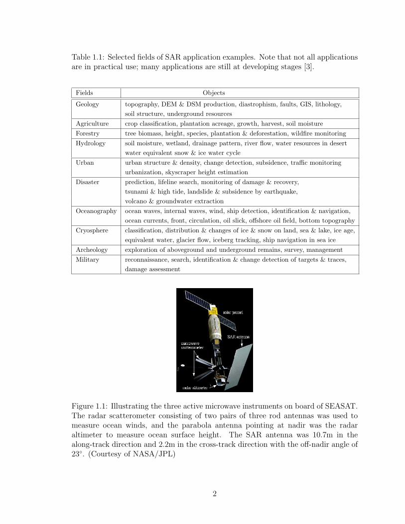
Table 1.1: Selected fields of SAR application examples. Note that not all applicationsare in practical use; many applications are still at developing stages [3].

Fields Objects

Geology topography, DEM & DSM production, diastrophism, faults, GIS, lithology,

soil structure, underground resources

Agriculture crop classification, plantation acreage, growth, harvest, soil moisture

Forestry tree biomass, height, species, plantation & deforestation, wildfire monitoring

Hydrology soil moisture, wetland, drainage pattern, river flow, water resources in desert

water equivalent snow & ice water cycle

Urban urban structure & density, change detection, subsidence, traffic monitoring

urbanization, skyscraper height estimation

Disaster prediction, lifeline search, monitoring of damage & recovery,

tsunami & high tide, landslide & subsidence by earthquake,

volcano & groundwater extraction

Oceanography ocean waves, internal waves, wind, ship detection, identification & navigation,

ocean currents, front, circulation, oil slick, offshore oil field, bottom topography

Cryosphere classification, distribution & changes of ice & snow on land, sea & lake, ice age,

equivalent water, glacier flow, iceberg tracking, ship navigation in sea ice

Archeology exploration of aboveground and underground remains, survey, management

Military reconnaissance, search, identification & change detection of targets & traces,

damage assessment

Figure 1.1: Illustrating the three active microwave instruments on board of SEASAT.The radar scatterometer consisting of two pairs of three rod antennas was used tomeasure ocean winds, and the parabola antenna pointing at nadir was the radaraltimeter to measure ocean surface height. The SAR antenna was 10.7m in thealong-track direction and 2.2m in the cross-track direction with the off-nadir angle of23◦. (Courtesy of NASA/JPL)

2

the techniques to utilize the wealth of potential information contained in the SAR data

[4]. At the time of SEASAT, intensity or amplitude images were of main interest, and

little consideration was given to preserving the phase in SAR processors. Of course,

amplitude data are the basis of SAR image analysis, and contain much information on

scattering media. Utilization of amplitude data is still a subject of current research.

The additional potential information suggested by SEASAT-SAR was the information

on the phase and polarization state in the coherently processed complex data.

The potential information in the phase of SAR complex images has led a new tech-

nology of interferometric SAR (InSAR). Today, InSAR is an established technology

operating on commercial basis as well as research basis in the fields of earth sci-

ence and technology. InSAR can be classified into two types, the cross-track InSAR

(CT-InSAR) and along-track InSAR (AT-InSAR). CT-InSAR is used for producing

topographic maps from the interferograms (interference patterns) produced by com-

plex data received by multiple antennas placed in the cross-track direction, or by a

single antenna with multiple orbits. By removing topographic effect, it can measure

crust movement caused by, for example, earthquakes and volcanic activity, and of

glacier movement [5, 6]. This type of InSAR is known as differential InSAR (DIn-

SAR). PS-InSAR (Permanent Scatterer InSAR) uses the temporal phase changes of

semi-permanent scatterers that always give rise to strong backscatter, and its mea-

surement accuracy is of the order of several millimeters per year [7, 8]. AT-InSAR

operates with multiple antennas placed in the along-track direction. The interfero-

grams contain information on the changes of Doppler center from the line-of-sight

component of scatterers’ velocity, and as such, AT-InSAR measures the velocity of

moving hard targets and ocean currents associated with, for example, tides and in-

ternal waves [9, 10].

The polarization information has lead another new technology of polarimetric SAR

3

(PolSAR) which is a considerable current interest [11, 12, 13, 14]. The principle of

PolSAR is to make use of the changes of polarization state between the transmitted

and received signals. The changes are caused by different scattering mechanisms by

different objects’ structure and material, and therefore, PolSAR can be used to dis-

tinguish the scattering objects and to improve image classification. Linearly polarized

microwave changes its polarization angle when it goes through dense electron clouds

in the ionosphere. It is known as ”Faraday effect”, and PolSAR can be a useful tool

for the investigation of such effect [15, 16, 17]. Attempts have also been made to com-

bine SAR polarimetry and interferometry. Pol-InSAR (polarimetric-interferometric

SAR), which is a subject of active current research, can be used to improve image

classification and to estimate tree height [18].

Thus, the pioneering SEASAT-SAR has guided us to establish a new paradigm

in radar remote sensing, and the state-of-the-art technologies developed in the new

paradigm are taking a central role in the wide range of fields of earth science and

engineering.

1.2 Selected Spaceborne and Airborne SAR

Table 1.2 lists selected spaceborne SARs. In the table, the values of spatial resolu-

tion are for the highest resolution possible (usually, spotlight/fine mode with single-

polarization). The standard mode is nominal standard or strip mode with single-look

images. Spatial resolution for fine mode or spotlight mode is higher than the stan-

dard mode at the expense of area coverage, and it is lower for the scan mode with the

advantage of wider area coverage. The azimuth resolution is often quoted by “mul-

tilook”. For example, the nominal azimuth resolution of ALOS-PALSAR (Advanced

Land Observing Satellite-Phased Array L-band SAR) is 4.5 m, but the standard prod-

4

Table 1.2: Parameters of selected spaceborne SARs. “Pol.” means the availablecombination of polarization states, “Res.” indicates the finest available spatial res-olutions in azimuth/range directions, “Weight” is in kg, and “Alt.” is the averageorbit altitude in km. The parentheses next to sensor name are the number of identicalsatellites.

Sensor name Agency Year Band Pol. Res.(m) Weight Alt.

SEASAT-SAR NASA 1978 L HH 6.25/25 2,290 800

ERS-1/2 ESA 1991/1995 C VV 5/25 2,400 785

JERS-1 JAXA 1992 L HH 6/18 1,400 570

RADARSAT-1 CSA 1995 C HH 8/8 3,000 798

ENVISAT-ASAR ESA 2002 C Dual 7.5/30 8,211 800

ALOS-PALSAR JAXA 2006 L Quad 4.5/9 3,850 692

Yaogan-SAR China 2006 L N/A 5/5 2,700 625

SAR-Lupe (5) Germany 2006-2008 X Quad 0.5/0.5 770 500

TerraSAR-X Germany 2007 X Quad 1/1 1,230 514

RADARSAT-2 CSA 2007 C Quad 3/3 2,200 798

Cosmo-SkyMed (4) Italy 2007-2010 X Quad 1/1 1,700 620

TecSAR Israel 2008 X Quad 0.1/0.1 300 515

RISAT-2 India 2009 X Quad 1/1 300 550

TanDEM-X Germany 2009 X Quad 1/1 1,230 514

RISAT-1 India 2012 C Quad 1/1 1,858 480

Sentinel-1 (3) ESA 2013- C Dual 5/5 2,300 693

ALOS-2 JAXA 2013 L Quad 1/3 2,000 628

KOMPSAT-5 Korea 2013 X Quad 1/1 1,400 550

SAOCOM 1A, 1B Argentine 2014-2015 L Quad 7/7 N/A 620

RADARSAT-Const. (3-6) CSA 2016-2017 C Quad 3/3 1,300 592

uct is in 2-look so that the azimuth resolution equals the slant-range resolution of 9

m. The resolution of PALSAR in the wide-swath scan mode becomes approximately

100m.

Since the launch of SEASAT-SAR, many spaceborne SARs have been put into orbit

by various organizations such as NASA, ESA, CSA and JAXA.

After the launch of SEASAT in 1978, scientists realized the potential of SAR in

variety of fields of geoscience and engineering. The second spaceborne SAR following

the SEASAT-SAR was the ERS-1 SAR in 1991. During the 13 years of interval be-

5

tween the SEASAT and the ERS-1, much effort was made to develop and experiment

new techniques with airborne SARs and Shuttle Imaging Radar (SIR) series aboard

the NASA Space Shuttle. The SIR-A mission was in 1981 with a L-band HH polar-

ization SAR similar to that of SEASAT. The SIR-B mission followed in 1984 with

SAR operating at the same frequency and polarization as the SIR-A, but varying

incidence angles by a mechanically steered antenna.

The SIR missions continued, and in 1994 the SIR-C/X-SAR was in orbit, which, for

the first time, operated at multi-frequency X-, C- and L-bands with a full polarimetric

mode. The Shuttle Radar Topography Mission (SRTM) in 2000 carried X- and C-

band main antennas on the cargo bay and a second outboard antenna separated by

a 60m long mast. With InSAR using the two antennas the SRTM produced a digital

elevation model (DEM) of approximately 80% of land.

Increasing number of spaceborne SARs has been launched recently and further mis-

sions are being planned. The general trends are that the spatial resolution is becoming

finer, and different beam modes are available including high-resolution Spotlight and

wide-swath Scan modes.

At L-band, the spatial resolution of SEASAT-SAR was 6 m in single-look azimuth

direction and 25 m in range direction; while that of ALOS-PALSAR, the newer L-

band spaceborne SAR, was 4.5 m in azimuth and 9 m in range directions. ALOS-

PALSAR completed its operations in May 2011 and as a successor of ALOS-PALSAR,

ALOS-2 will be launched in Nov. 2013 and it will achieve 1 m in azimuth and 3 m

in range resolutions in the Spotlight mode [19, 20]. The Chinese Yaogan series are

highly classified, but allegedly several Yaogans equipped with SAR were launched

and newer series are expected to have around 1 m resolution.

At X-band, the German TerraSAR-X and the Italian civil and military Cosmo-

6

SkyMed have achieved 1 m resolution in both directions. Even finer resolution of 0.5

m has been achieved by the German reconnaissance SAR-Lupe. The fine resolutions

of the latter three SARs are in the Spotlight mode. TerraSAR-X and TanDEM-X

fly as a pair of several hundreds meter apart to constantly genarate global Digital

Elevation Model (DEM) using InSAR technique.

While higher frequency band such as X-band is favorable in achieving higher spatial

resolution, the SARs operating at the low frequency band such as L- and P-bands

have relatively long penetration depth into forests, vegetation, soil and ice. Table 1.3

lists the radar bands and corresponding frequencies and wavelengths. The names of

radar bands originated in World War II and have been customarily used since then.

For instance, the name of “P” comes from “Previous” radar, “L” and “S” stand

for “Long” and “Short” respectively, and “C” is “Compromise” between S- and X-

bands. SAR images are strongly affected by the wavelength of microwaves. For

example, longer wavelengths, such as L- or P-band is more suitable for investigating

forests than shorter wavelengths such as X- or C-band, because longer wavelength

microwaves can penetrate deeper into forest interior, providing more information of

the forests. Also, surface roughness, to a given wavelength, is “effective” roughness.

In other words, surface roughness is defined according to a radar wavelength. For

example, a surface can be “rough” for X-band, while it can be “smooth” for L-band.

Thus, a same surface may appear differently in SAR images.

Employing spaceborne SARs at lower altitude is another way to improve spatial

resolution, but this results in shorter life-span because of the effect of stronger gravity.

There are also many airborne SARs developed by various organizations, and almost

all systems operate at multi-frequency full polarization mode with CT- and/or AT-

InSAR functions. The well-known airborne SARs include AIRSAR (X- C-, L-, P-

bands), E-SAR (X-, C-, S-, L-, P-bands) of DLR, Danish EMISAR (C-, L-bands),

7

Table 1.3: Common frequency bands for radar systems.

Radar band Frequency (GHz) Wavelength (cm)

VHF 0.03-0.3 1000-100P 0.3-1 100-30L 1-2 30-15S 2-4 15-7.5C 4-8 7.5-3.8X 8-12.5 3.8-2.4Ku 12.5-18 2.4-1.67K 18-26.5 1.67-1.1Ka 26.5-40 1.1-0.75Q 40-60 0.75-0.5V 50-75 0.6-0.4W 75-110 0.4-0.27

Pi-SAR (X-, L-bands) of NICT/JAXA, SAR580 (X-, C-bands) of CCRS and Swedish

CARABAS-II SAR (VHF-Ultra Wide Band). Table 1.4 lists selected airborne SARs.

The spatial resolutions of them are the order of meters or less.

1.3 Other Recent Trends in SAR

One of the other recent trends is the lighter weights of spaceborne SARs. Lighter

weight is advantageous for easier platform launch and longer SAR life-span. The very

first SEASAT-SAR weighed approximately 2.3 tons, while the recent TecSAR is mere

0.3 tons. The heaviest spaceborne SAR ever launched was ENVISAT which weights

approximately 8.2 tons; the Japanese ALOS was the second-heaviest with 3.85 tons.

The main reason for the heavy weight is that the satellite carries many sensors on

board. ENVISAT, for example, carries 10 optical/infrared and microwave instruments

including ASAR (Advanced SAR), and ALOS carries PALSAR and other two optical

sensors. Cosmo-SkyMed, TerraSAR-X and SAR-Lupe are ”SAR-only” satellites, and

8

Table 1.4: Parameters of selected airborne SARs. “Res.” indicates the maximumachievable spatial resolutions in azimuth/range directions. Most of the listed airborneSARs operate in quad- (quadrature) polarization with interferometric modes. UAVnext to sensor name stands for Unmanned Aerial Vehicle.

Sensor name Agency (Country) Band Res.(m)

C/X-SAR CCRS (Canada) X/C 0.9/6

AIRSAR NASA/JPL (US) X/C/L/P 0.6/3

E-SAR DLR (Germany) X/C/S/L/P 0.3/1

Pi-SAR NICT/JAXA (Japan) X/L 0.37/3

EMISAR DCRS (Denmark) C/L 2/2

PHARUS TNO-FEL (Netherlands) C 1/3

RAMSES ONERA (France) W/Ka/Ku/X/C/S/L/P 0.12/0.12

CARABAS-II FOA (Sweden) VHF 3/3

XWEAR Defence R&D (Canada) X Wide-band < 1

Lynx (UAV) Sandia (US) Ku 0.1/0.1

Global Hawk (UAV) Northrop Grumman (US) X 1.8/1.8

UAVSAR (UAV) NASA/JPL (US) L 0.5/1.8

PicoSAR (UAV) SEGG/SELEX (Austria/Italy) X 0.05/0.05

as such their weights are considerably reduced.

These SAR-only satellites are compact, and several SARs of the same type can be

put into orbit. This in turn reduces the revisit periods which have been one of the

major problems in satellite remote sensing. There are four identical Cosmo-SkyMed

SARs and five SAR-Lupe SARs, with their revisit period of 12 hours and less than

10 hours respectively, as compared with, for example, 44 days of JERS-1 SAR. If

14 identical SARs were used, the revisit time would be 1 hour, and it would be 10

minutes for 36 SARs.

1.4 Purpose of This Study

Along with the trends mentioned so far, the conventional single-polarization mode is

getting replaced by dual or full polarimetric modes. With increased quality of SAR

9

systems utilizing polarimetric information recently, the development and applications

of PolSAR are one of the current major topics in radar remote sensing. While con-

ventional SAR systems handle only single polarimetric information, data acquired

through PolSAR systems contain fully polarimetric information on the shift in po-

larization between the transmitted and received microwave. They have potential to

increase further the ability of extracting physical quantities of the scattering targets.

Therefore, they are used in broad fields of study such as visualization for classification

[21, 22], oil-slick detection [23, 24], and ship detection [25, 26, 27], to name a few.

Several decomposition techniques have been proposed along with the utilization of

fully polarimetric data (i.e. quad-polarization data) provided by PolSAR systems.

Many of them can be categorized into either of two main groups. One is based on

eigenvalue analysis [11, 13, 28], and the other employs scattering model-based decom-

position originally proposed by Freeman and Durden [14]. The basic idea behind the

model-based decomposition is that the backscattering power can be expressed as a

linear sum of three different scattering power components.

On the other hand, while quad-polarization data seem to be promising considering

the abundance of information on targets, it is also important to suggest suitable

analytical methods within the trade-offs between purposes, situations, available data

sets, and available polarization.

The purpose of this study is to contribute to deeper understanding of SAR polarime-

try by experimenting and validating PolSAR methodology for SAR image analyses,

by suggesting practical applications focusing on target detection and by comparing

various PolSAR analytical methods with different polarizations.

10

1.5 Outline of the Thesis

The outline of the thesis is illustrated in Figure 1.2. In Chapter 1, SAR origin,

progress, applications, achevements, and recent trends are introduced and the pur-

pose of this study is stated. In Chapter 2, SAR fundamentals, i.e., SAR image

forming processes including the pulse compression technique and aperture synthesis

technique are introduced. In Chapter 3, the fundamentals of electromagnetic wave

polarization are described and well known analytical methods for SAR polarimetry

are introduced. Chapter 1-3 are for providing background knowledge about the disser-

tation. In Chapter 4, the four-component scattering power decomposition (4-CSPD)

algorithm with rotation of covariance matrix is introduced. The 4-CSPD is one of

the model-based decomposition algorithms and recently a rotation scheme is intro-

duced to improve classification results in urban areas. In Chapter 5, the eigenvalue

analysis with dual-polarization data is compared with the eigenvalue analysis with

quad-polarization data. In Chapter 6, man-made targets on the sea are detected

using the result of model-based decomposition effectively. In Chapter 7, the detec-

tion reaults of laver cultivation nets are compared by using common polarimetric

analytical methods comprehensively.

11

Figure 1.2: Outline of the thesis

12

Chapter 2

SAR Fundamentals

In this chapter, SAR image formation processes are introduced. SAR is an imaging

radar which produces high-resolution two-dimensional radar images by synthesizing

a large aperture in azimuth (along-track) direction utilizng the Doppler effect and a

small antenna on board a satellite/aircraft, and by using FM (Frequency Modulation)

pulses and the pulse compression technique in range direction [1, 2, 29, 30, 31].

Attempts to acquire Earth’s information in global scale from SAR data started

since the launch of SEASAT-SAR in 1978. Since then, a large amount of research and

experiments have been carried out and much progress has been made in fundamental

research, algorithm development, image analysis and applications to many fields of

geoscience. Synthetic aperture processing is an established technique now, but how

to extract useful information from SAR data is still in a developing stage.

This chapter is organized as follows. First, radar system parameters are introduced.

Then the techniques of pulse compression and aperture synthesis used in SAR system

to achieve high resolution are presented.

13

2.1 SAR System Parameters

SAR data are produced from the return echoes (microwaves) which are emitted by

a SAR transmitter, reflected from ground targets, and received by a SAR receiver.

Thus, they are dependent on SAR system parameters and target characteristics. To

understand information contained in SAR data, the system parameters should be

understood first. Common system parameters are described in the following subsec-

tions.

2.1.1 Geometry of SAR System

Figure 2.1 shows the basic geometry of a SAR system [1, 2, 30]. A platform at an al-

titude h carries a side-looking radar antenna that illuminates the Earth’s surface with

pulses of electromagnetic waves. The direction of moving platform is called azimuth

direction or along-track direction, and the direction of the transmitted electromag-

netic pulses, which is orthogonal to azimuth direction, is called range direction or

cross-track direction. There are two ways to represent range direction. Slant-range

direction is from the antenna to illuminated ground targets, while ground-range di-

rection is slant-range direction projected on the Earth’s surface. R0 is the shortest

distance from the antenna to the ground targets and it can be accurately measured

from the time interval between pulse transmission and reception.

In the illuminated area, the side closest to the antenna is called near-range and

the side farthest from the antenna is called far-range. Swath width is the width

between near-range to far-range. Off-nadir angle θo is the angle between slant-range

direction and a direction perpendicular to the Earth’s surface from the platform.

Incidence angle θi is defined as the angle between slant-range direction and a normal

14

from Earth’s surface where the illuminated targets are located. The incidence angle

varies through swath width, and generally quoted incidence angle (nominal incidence

angle) is that at the center of the image swath. The incidence angle is an important

parameter for its impact on the radar backscatter and geometrical effects [1, 13, 32,

33].

slant-range

direction

ground-range

direction

incidence angle

platform

azimuth direction

off-nadir angle θ

i

o

swath width

far-range

near-range

hR

0

θ

travel direction

Figure 2.1: Illustration of SAR geometry.

2.1.2 Signal Parameters

There are three important parameters that describe the characteristics of transmit-

ted pulses. They are pulse duration (length) τp, bandwidth B and pulse repetition

frequency (PRF) fp [30]. Since the pulse transmission and reception times cannot

15

Figure 2.2: Pulses and observation window of spaceborne SAR. fp is pulse repetitionfrequency, tp is pulse repetition time and the inverse number of fp, and τw is thetime duration of the observation window. The observation window is for the firsttransmitted pulse.

overlap, the swath width is restricted by fp as follows:

slant-range swath width <c

2× fp(2.1)

where c is the speed of light. For airborne SARs, the maximum slant-range distance

is several tens of km, which is shorter than the slant-range of spaceborne SARs and a

return signal is received before the next pulse transmission. However, for spaceborne

SARs, slant-range is very long and a return signal is received not before the next

pulse transmission but after several pulse transmissions as shown in Figure 2.2.

The other important signal parameter is wavelength λ, which is related to the radar

frequency f0 (in Hz) by

λf0 = c (2.2)

2.2 Image Formation in Range Direction

Most imaging radars, including real aperture radars (RAR) and SAR, achieve high

resolution in range direction by using the pulse compression technique. Before the

16

pulse compression technique was invented, conventional rectangular pulses without

frequency modulation were used to produce radar images. In this section, the image

formation processes with rectangular pulses and with the pulse compression technique

are described.

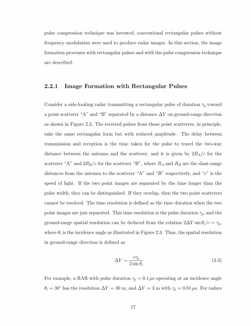
2.2.1 Image Formation with Rectangular Pulses

Consider a side-looking radar transmitting a rectangular pulse of duration τp toward

a point scatterer “A” and “B” separated by a distance ∆Y on ground-range direction

as shown in Figure 2.3. The received pulses from those point scatterers, in principle,

take the same rectangular form but with reduced amplitude. The delay between

transmission and reception is the time taken for the pulse to travel the two-way

distance between the antenna and the scatterer, and it is given by 2RA/c for the

scatterer “A” and 2RB/c for the scatterer “B”, where RA and RB are the slant-range

distances from the antenna to the scatterer “A” and “B” respectively, and “c” is the

speed of light. If the two point images are separated by the time longer than the

pulse width, they can be distinguished. If they overlap, then the two point scatterers

cannot be resolved. The time resolution is defined as the time duration when the two

point images are just separated. This time resolution is the pulse duration τp, and the

ground-range spatial resolution can be deduced from the relation 2∆Y sin θi/c = τp,

where θi is the incidence angle as illustrated in Figure 2.3. Thus, the spatial resolution

in ground-range direction is defined as

∆Y =cτp

2 sin θi(2.3)

For example, a RAR with pulse duration τp = 0.1µs operating at an incidence angle

θi = 30◦ has the resolution ∆Y = 30 m, and ∆Y = 3 m with τp = 0.01µs. For radars

17

with rectangular pulses, the shorter the pulse duration is, the finer the resolution

becomes. The resolution also becomes coarse as the incidence angle decreases, and

∆Y → ∞ in the limit of θi → 0. This is the reason why the imaging radar is

side-looking.

A B

θi

A B

Figure 2.3: Illustrating range imaging process and resolution of a conventional radarwith rectangular pulses.

2.2.2 Image Formation with the Pulse Compression Tech-

nique

In the conventional technique based on rectangular (non-chirp) pulses, resolution

improves as pulse duration becomes shorter. However, there is a limit to continu-

ously generate high-power short pulses using onboard power supply for airborne and

spaceborne SARs. To overcome this problem, the pulse compression technique was

developed. In this technique, high resolution in range direction can be achieved by

using frequency modulated (FM) or chirp pulses of long duration, and by applying

appropriate signal processing to received pulses. In particular, for spaceborne SARs

18

whose power supply is from solar panels, the pulse compression technique is essential

and a must. Most of recent airborne SARs also use the pulse compression technique

to achieve high resolution in range direction. A unique characteristic of the pulse

compression technique is that higher resolution can be achieved with longer pulse

duration, contrary to the conventional non-chirp radars.

FM pulse or chirp pulse is a pulse whose frequency changes linearly with time τ .

The FM pulse (transmitted signal) is defined as follows [1, 2, 30].

Et(τ) = E ′0 exp(iωcτ+iατ

2) : |τ | ≤ τp/2 (2.4)

where E ′0 denotes the amplitude of the transmitted signal, ωc denotes the center

radian frequency, α is the chirp constant, α/π is called chirp rate or FM rate, and

τp is the pulse duration. Without a loss of generality, a complex expression is used

in Equation (2.4). In practice, the transmitted and received pulses are in a real

form, but after pulse reception the real signal is transformed into a complex signal by

filtering. It should be noted that in many fields of science and engineering, complex

expressions are adopted and the real component is taken from the final expression

because of the mathematical complexity of using trigonometric functions. The phase

of a charp pulse is ψ(τ) = ωcτ+ατ2, and therefore the instantaneous frequency f can

be derived as

f(τ) =1

2π

dψ

dτ

= fc +ατ

π(2.5)

and the charp bandwidth BR can be given as

BR = |α|τp/π (2.6)

19

f (τ)

Real{Et(τ)}

-τp/2 τ τp/20 (a)

(b) τp/2 τ

-τp/2

0

Figure 2.4: Illustrating (a) the real component of the phase of a FM pulse and (b)instantaneous frequency with ωc = 0.

The frequency of the chirp pulse varies linearly with time with the gradient α/π.

The gradient is the chirp rate. Figure 2.4 illustrates the charp pulse when the center

frequency is 0 Hz. For JERS-1 SAR, α/π = −4.3 × 1011 Hz/s, τp = 35.2 µs, BR =

15 MHz, fc = 1275 MHz, and λ = c/fc = 0.235 m. The positive chirp rate is called

up-chirp and the negative chirp rate is called down-chirp. Note that the word “chirp”

stems from “birds’ chirp” in which birds chirp with increasing frequency.

The received signal from a point scatterer at a distance R0 from the antenna takes

20

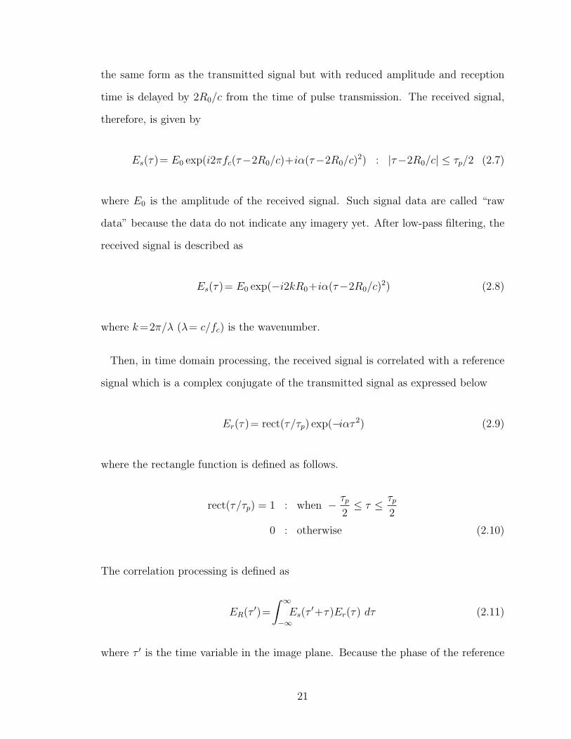
the same form as the transmitted signal but with reduced amplitude and reception

time is delayed by 2R0/c from the time of pulse transmission. The received signal,

therefore, is given by

Es(τ)= E0 exp(i2πfc(τ−2R0/c)+iα(τ−2R0/c)2) : |τ−2R0/c| ≤ τp/2 (2.7)

where E0 is the amplitude of the received signal. Such signal data are called “raw

data” because the data do not indicate any imagery yet. After low-pass filtering, the

received signal is described as

Es(τ)= E0 exp(−i2kR0+iα(τ−2R0/c)2) (2.8)

where k=2π/λ (λ= c/fc) is the wavenumber.

Then, in time domain processing, the received signal is correlated with a reference

signal which is a complex conjugate of the transmitted signal as expressed below

Er(τ)= rect(τ/τp) exp(−iατ 2) (2.9)

where the rectangle function is defined as follows.

rect(τ/τp) = 1 : when − τp2

≤ τ ≤ τp2

0 : otherwise (2.10)

The correlation processing is defined as

ER(τ′)=

∫ ∞

−∞Es(τ

′+τ)Er(τ) dτ (2.11)

where τ ′ is the time variable in the image plane. Because the phase of the reference

21

signal is “matched” to the phase of the complex conjugate of the charp (transmitted)

signal, the correlation processing of equation (2.11) is called “matched filtering” in

time domain. In actual SAR processors, the matched filtering is carried out in the

frequency domain so as to produce images from raw data in range direction, i.e., the

received signal is Fourier transformed, multiplied by the reference spectrum which is

the Fourier transform of the reference signal, and finally the resultant image spectrum

is inverse Fourier transformed to produce the image in time (or equivalent space)

domain. Here, the matched filtering is introduced in time domain because it is much

easier to explain the correlation operation in the time domain. The details of the

matched filtering in the frequency domain can be found in [1].

The integral of Equation (2.11) can be solved as

ER(τ′)=E0 exp(−i2kR0)(τp−|τ ′−2R0/c|) sinc[(α(τ ′−2R0/c)(τp−|τ ′−2R0/c|))]

(2.12)

where the sinc function is defined as sinc(z) = sin(z)/z. The image plane (origin) of

equation (2.12) is at the antenna (the time of pulse transmission). It is convenient

to change the origin of the time variable to the image plane at slant-range 2R0/c as

follows (also shown in Figure 2.5).

τR=τ′−2R0/c (2.13)

Equation (2.12) can then be written in a simpler form

ER(τR)=E0 exp(−i2kR0)(τp−|τR|)sinc (ατR(τp−|τR|)) (2.14)

ER is a complex image amplitude of a point scatterer and is called point spread

22

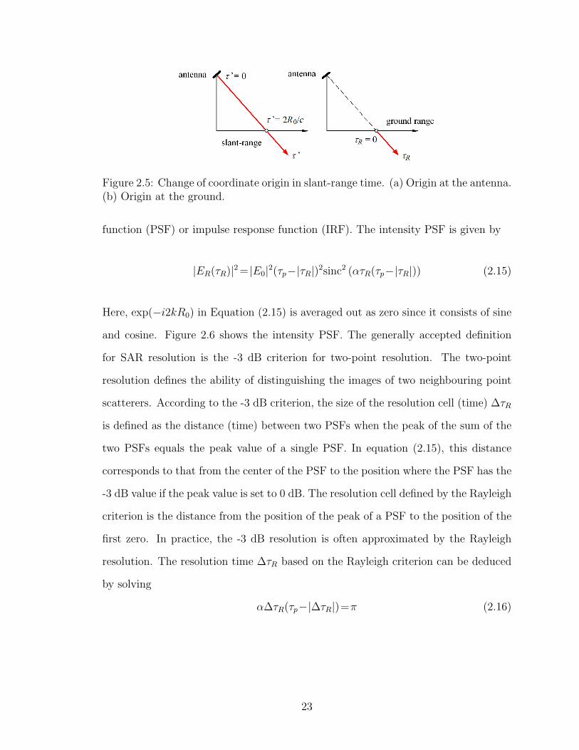
Figure 2.5: Change of coordinate origin in slant-range time. (a) Origin at the antenna.(b) Origin at the ground.

function (PSF) or impulse response function (IRF). The intensity PSF is given by

|ER(τR)|2= |E0|2(τp−|τR|)2sinc2 (ατR(τp−|τR|)) (2.15)

Here, exp(−i2kR0) in Equation (2.15) is averaged out as zero since it consists of sine

and cosine. Figure 2.6 shows the intensity PSF. The generally accepted definition

for SAR resolution is the -3 dB criterion for two-point resolution. The two-point

resolution defines the ability of distinguishing the images of two neighbouring point

scatterers. According to the -3 dB criterion, the size of the resolution cell (time) ∆τR

is defined as the distance (time) between two PSFs when the peak of the sum of the

two PSFs equals the peak value of a single PSF. In equation (2.15), this distance

corresponds to that from the center of the PSF to the position where the PSF has the

-3 dB value if the peak value is set to 0 dB. The resolution cell defined by the Rayleigh

criterion is the distance from the position of the peak of a PSF to the position of the

first zero. In practice, the -3 dB resolution is often approximated by the Rayleigh

resolution. The resolution time ∆τR based on the Rayleigh criterion can be deduced

by solving

α∆τR(τp−|∆τR|)=π (2.16)

23

-5π

|E |R2

0

1

ΔY

・・・・・・・・・・・・

5ππ 2π 3π 4π-π-4π -3π -2ππY

Figure 2.6: Intensity point spread function in range direction.

As a result, the resolution time ∆τR is

∆τR =τ02

(1−

√1− 4

τ0BR

)(2.17)

where the product of the pulse duration and bandwidth

TBP = τ0BR (2.18)

is called TBP (time bandwidth product). The TBP of general SAR systems is large.

For JERS-1 SAR, τ0BR = 35.2(µs) × 15(MHz) = 528. For large TBP (τpBR ≫ 1),

the pulse compression ratio (ratio of pulse duration τp to the resolution time ∆τR)

24

can be approximated as follows.

τ0∆τR

= τ0BR (2.19)

Therefore,

∆τR =1

BR

=1

|α|τp/π(2.20)

This means higher resolution can be achieved with increasing pulse duration as op-

posed to RAR such as SLAR. For large TBP, the complex PSF and intensity PSF

can respectively be approximated using the fact that τ0 ≫ ∆τR as follows.

ER(τR)=E0 exp(−i2kR0)τpsinc (πBRτR) (2.21)

|ER(τR)|2= |E0|2τ 2p sinc2 (πBRτR) (2.22)

Since it is more practical to express SAR images in space domain (ground-range)

rather than time domain (slant-range), we put Y sin θi = cτR/2. Then, the complex

PSF and intensity PSF can be expressed respectively by

ER(Y )=E0 exp(−i2kR0)sinc (πY/∆Y ) (2.23)

|ER(Y )|2= |E0|2sinc2(πY/∆Y ) (2.24)

where Y is ground-range variable (distance). Note that τp in Equation (2.21), (2.22)

is now included in E0. and the resolution cell (the spatial resolution in ground-range

direction) is defined by

∆Y =c

2BR sin θi=

πc

2|α|τp sin θi(2.25)

This is the resolution listed in Table 1.2, 1.4. For example, for JERS-1 SAR with τ0 =

25

35.2 µs and at the incidence angle θi = 41◦, the resolution without pulse compression

is approximately 8.2 km. If the pulse compression technique is used, the resolution

improves to 16 m. In summary, the following can be said from Equation (2.25)

• On the contrary to the case of non-chirp pulses, resolution ∆Y improves as

pulse duration τ0 becomes longer.

• Resolution degrades (worsens) as incidence angle θi decreases in the same way

as non-chirp pulses.

• Finer resolution can be achieved with increasing chirp rate α.

2.3 Image Formation in Azimuth Direction

2.3.1 Image Formation with Real Aperture Radar

In azimuth direction, the resolution is determined by the beam width. As shown in

Figure 2.7, the signal from the scatterer “A” is just separated from the signal from

“B” is when the two scatterers are separated by the distance of the azimuth beam

width. This is the case with ideal uniform antenna illumination (amplitude) pattern.

Since actual beam pattern is not uniform, the definition of resolution in Figure 2.7

is not practical. Thus, the beam pattern needs to be introduced first. The absolute

amplitude value can be expressed as

WA(p) =

∣∣∣∣sinc(kDA

2Rc

p

)∣∣∣∣ (2.26)

where DA is the antenna length, p is azimuth space variable (platform position), Rc is

an arbitrary slant-range distance and it becomes Rc = R0 at the coordinate origin of

26

illuminated plane as shown in Figure 2.8(a). The beam width, L0, can be expressed

as

L0 ∼2λRc

DA

(2.27)

Figure 2.8(b) shows resolution of a power image in azimuth direction by the Rayleigh

criterion. Therefore, the azimuth resolution of real aperture radars is defined by

∆X = L0/2 (2.28)

Since the antenna length and the beam width are inversely proportional, a extremely

long antenna is required to achieve the azimuth resolution of a similar order of the

range resolution. For the JERS-1 SAR, the antenna length DA = 12 m, wavelength

λ = 0.235 m, and the slant-range distance R = 750 km. The azimuth resolution

∆X would be approximately 15 km if it is operated as a RAR. The range resolution

of JERS-1 SAR was approximately 18 m and to obtain the same azimuth resolution

with RAR, the antenna length would have to be approximately 10 km.

In azimuth direction, fairly fine resolution can be achieved for airborne radars by

using a long antenna, but spaceborne radars such as JERS-1 SAR cannot be operated

as RAR because of the limitation to the antenna size and hence very coarse resolution.

In order to obtain fine azimuth resolution, the technique known as “aperture synthe-

sis” [2] is adopted for the modern airborne and spaceborne radars. Indeed, the name

“synthetic aperture radar” stems from this technique of synthesizing a large virtual

aperture (i.e. a very long virtual antenna) with a small antenna and appropriate

processing of received signals.

27

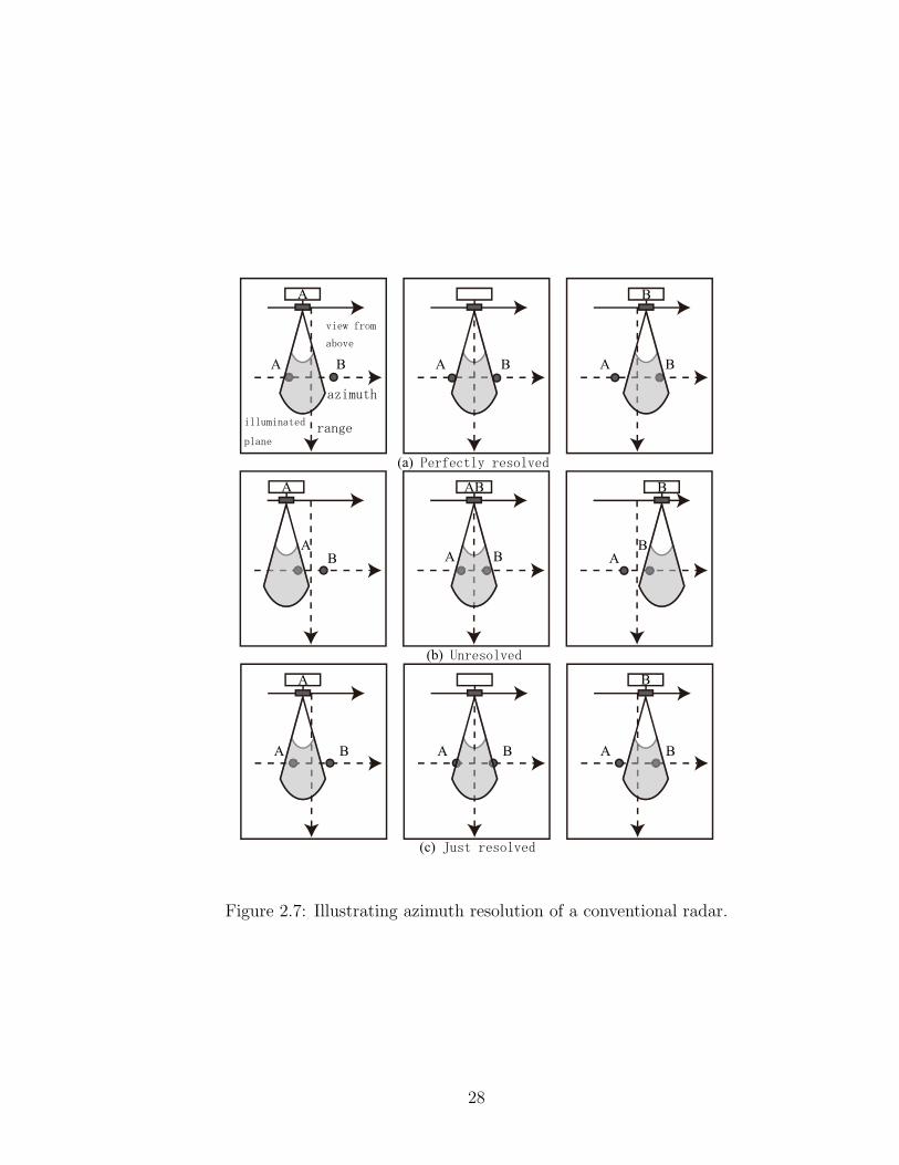
(a)

(b)

(c)

A B A B A B

AB BA

BA

A B A B A B

A B

A AB B

A B

Figure 2.7: Illustrating azimuth resolution of a conventional radar.

28

λR /Dc A

-λR /Dc A λR /Dc A

DA

Rc

R0

X

(a)

(b)

Figure 2.8: (a) Beam pattern in azimuth direction. (b) Resolution: in the case of sincfunction beam pattern.

29

R0

travel speed V

Az

Rn

R

t=t

platform

t=0

Figure 2.9: Illustration of a geometry of a point scatterer and the platform at differentazimuth times.

2.3.2 Image Formation with Aperture Synthesis

In the preceding section, the range PSF is derived for a point scatterer at a fixed range

R0. However, the SAR antenna transmits and receives series of pulses as it travels

in azimuth direction. As shown in Figure 2.9, consider that the antenna on board of

a satellite or aircraft platform at an arbitrary azimuth time t transmits and receives

signals from a point scatterer at the distance R, where V is the platform speed. The

distance R0 is the slant-range distance when the antenna is nearest to the scatterer.

In the aperture synthesis technique, many range compressed signals are used in order

to achieve high azimuth resolution. The azimuth component of a received signal is

also frequency modulated as a chirp signal. Therefore, high resolution in azimuth

direction can be achieved by utilizing Doppler effect caused by the movement of a

radar antenna and by correlating received signals with expected reference signals. As

a result, a fine image can be produced. In practice, signal processing is carried out

in the frequency domain in most processors. Let the PRF be fp, then a transmitted

30

chirp pulse can be written as follows.

Et(τ)= E ′0 exp(i2πfc(tj + τ)+iα(tj + τ)2) (2.29)

where tj (j = 1, 2, 3, ...) is the j th pulse transmission time related to the PRT

(Pulse Repetition Time) by

tp = 1/fp = tj+1 − tj (2.30)

The time of signal reception from a point scatterer is delayed by the time 2rj/c from

the time of pulse transmission where rj is slant-range distance between an antenna

and a scatterer at j th pulse. Therefore, a received signal is expressed in the following

equation.

Es(τ)= E0 exp(i2πfc(tj + τ − 2rj/c)+iα(tj + τ − 2rj/c)

2)

(2.31)

Strictly speaking, this equation implicitly includes the antenna patternWA(t), but for

simplicity, a uniform antenna pattern is assumed. The equation also assumes that the

antenna positions of pulse transmission and reception are the same. In real situation,

the antenna moves between the times of pulse transmission and reception, and it is

necessary to add this time difference to the received signal. However, its effects are

slight and negligible on image defocus and a constant positional shift (approximately

10 m) of the entire image can easily be corrected. These effects can therefore be

safely ignored. This approximation is called stop-and-go model. The term involving

i2πfc(tj+τ) is removed after transforming the received signal into an offset frequency,

so that it is removed at this stage. The received signal can then be written as

Es(τ)= E0 exp (−i2kr(tj)) exp(iα(tj + τ − 2r(tj)/c)

2)

(2.32)

31

Figure 2.10: Aligned received pulses.

Next, the received pulses are re-arranged in the order of the pulse transmission time

as shown in Figure 2.10. Then, tj is removed from the phase of chirp pulses, and the

signal can be expressed in 2-D (dimentional) as follows.

Es(tj, τ)= E0 exp (−i2kr(tj)) exp(iα(τ − 2r(tj)/c)

2)

(2.33)

Figure 2.11 shows the top view of the re-arranged signal. The range and azimuth

times are of the order of speed of light and platform respectively, and hence they

are called the fast time and slow time. The skewness of the figure is observed by

spaceborne SARs and is caused by the Earth’s daily rotation. It is called range

skew. For airborne SARs, a re-arranged signal is almost symmetrical. After range

compression under large TBP, the signal becomes

E ′s(t, τ

′)= E0 exp (−i2kr(t)) sinc (πBR(τ′ − 2r(t)/c)) (2.34)

In this 2-D signal, τ ′ is the time variable in range direction in the image plane. Also,

since fp satisfies the sampling theorem, the discrete time variable tj has been replaced

by a continuous time variable t. Figure 2.12 shows a 2-D signal after the range

compression. Since the distance between the antenna and a point scatterer changes

32

Figure 2.11: Top view of the re-arranged 2-D signal.

as the platform moves in azimuth direction, the range position of PSF also changes in

azimuth time. This effect is known as the range migration. The effect increases with

increasing resolution and with increasing radar wavelength. The relation between the

slant-range distance r(t) and azimuth time t is

r(t) = (R0 + vEt)2 + (V t)2 (2.35)

where R0 is the slant-range distance when the antenna is abeam of the scatterer

(t = 0), vE is the slant-range velocity component associated with the Earth’s rotation.

Let the illuminating time be T0, and then under the condition R0 + vEt ≫ V T0, the

following approximation holds.

r(t) =√(R0 + vEt)2 + (V t)2

≃ R0 + vEt+(V t)2

2(R0 + vEt)(2.36)

33

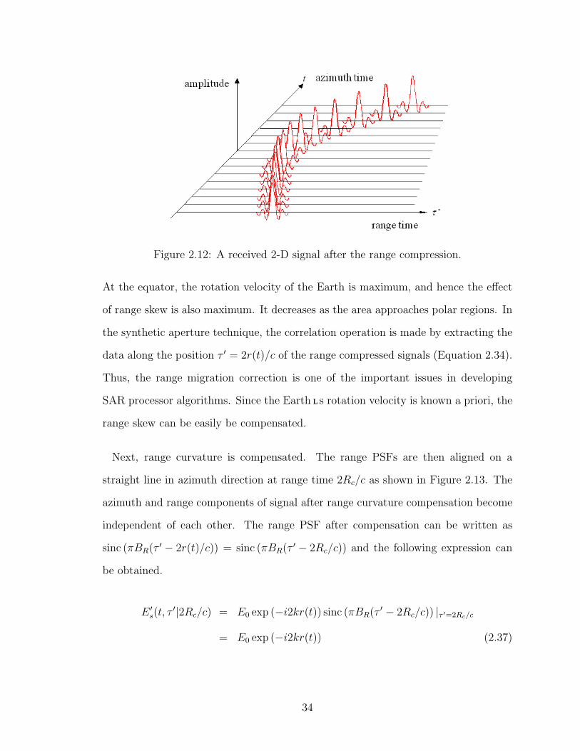
Figure 2.12: A received 2-D signal after the range compression.

At the equator, the rotation velocity of the Earth is maximum, and hence the effect

of range skew is also maximum. It decreases as the area approaches polar regions. In

the synthetic aperture technique, the correlation operation is made by extracting the

data along the position τ ′ = 2r(t)/c of the range compressed signals (Equation 2.34).

Thus, the range migration correction is one of the important issues in developing

SAR processor algorithms. Since the Earth’s rotation velocity is known a priori, the

range skew can be easily be compensated.

Next, range curvature is compensated. The range PSFs are then aligned on a

straight line in azimuth direction at range time 2Rc/c as shown in Figure 2.13. The

azimuth and range components of signal after range curvature compensation become

independent of each other. The range PSF after compensation can be written as

sinc (πBR(τ′ − 2r(t)/c)) = sinc (πBR(τ

′ − 2Rc/c)) and the following expression can

be obtained.

E ′s(t, τ

′|2Rc/c) = E0 exp (−i2kr(t)) sinc (πBR(τ′ − 2Rc/c)) |τ ′=2Rc/c

= E0 exp (−i2kr(t)) (2.37)

34

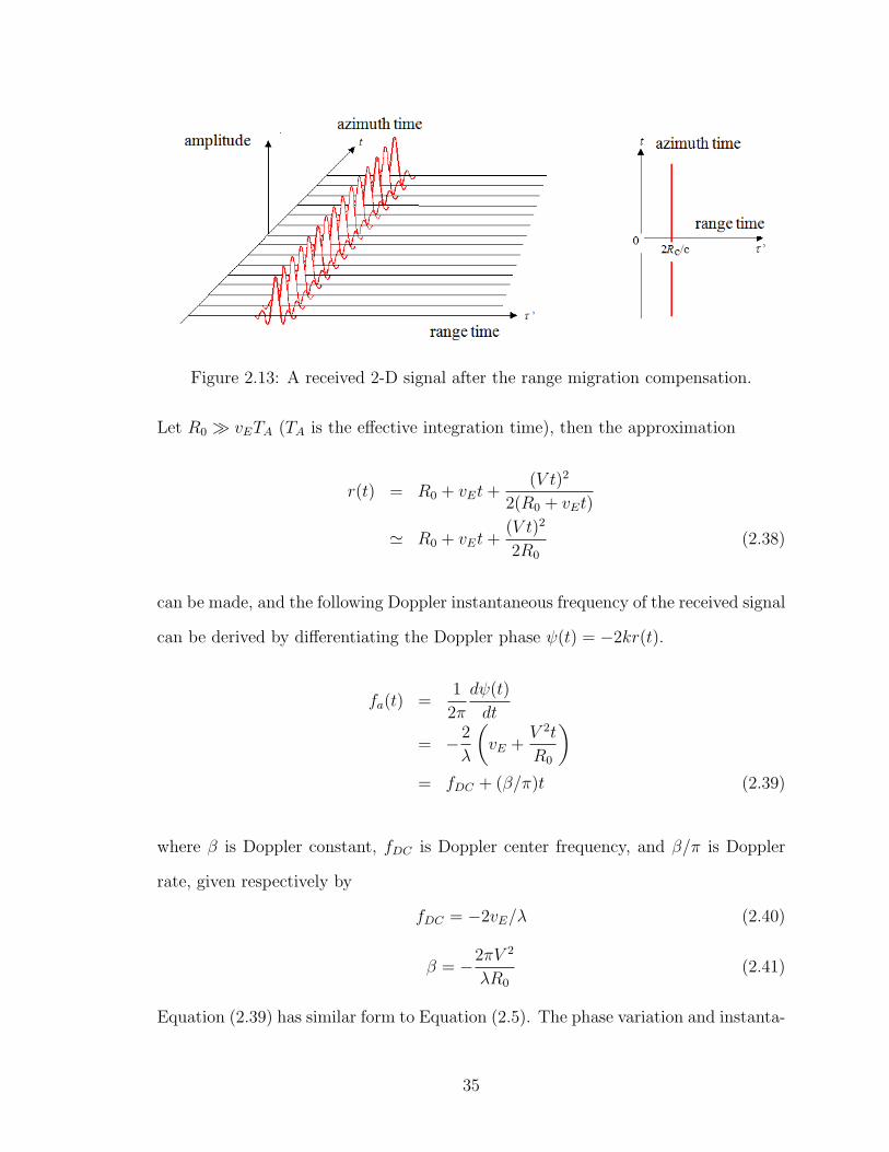
Figure 2.13: A received 2-D signal after the range migration compensation.

Let R0 ≫ vETA (TA is the effective integration time), then the approximation

r(t) = R0 + vEt+(V t)2

2(R0 + vEt)

≃ R0 + vEt+(V t)2

2R0

(2.38)

can be made, and the following Doppler instantaneous frequency of the received signal

can be derived by differentiating the Doppler phase ψ(t) = −2kr(t).

fa(t) =1

2π

dψ(t)

dt

= −2

λ

(vE +

V 2t

R0

)= fDC + (β/π)t (2.39)

where β is Doppler constant, fDC is Doppler center frequency, and β/π is Doppler

rate, given respectively by

fDC = −2vE/λ (2.40)

β = −2πV 2

λR0

(2.41)

Equation (2.39) has similar form to Equation (2.5). The phase variation and instanta-

35

neous Doppler frequency of the Doppler signal correspond to those of the chirp signal

used for range compression although the values are different. Thus, the received sig-

nal in azimuth direction is also frequency modulated chirp signal. The difference is

that the frequency modulation in range direction is made by the transmitted charp

signal itself, and the frequency modulation in azimuth direction is due to the change

in distance between the antenna and the scatterer. For JERS-1 SAR, V = 7 km/s,

R0 = 750 km, λ = 0.235 m, T0 = 2.1 s, and then the Doppler rate β/π is −556 Hz/s.

The center frequency at the equator is fDC ≃ −2.5 kHz and approaches zero as closer

to the polar regions. The Doppler bandwidth is defined as follows.

BA = |β|T0/π

=2V 2

λR0

T0 (2.42)

Since the Doppler bandwidth of received signal is defined as the 3 dB bandwidth of

the beam pattern, the real bandwidth is wider than the nominal value given above.

High resolution in azimuth direction is achieved by correlating the received signal

E ′s(t) = E0 exp(−i2kR0) exp(i2πfDCt+ iβt2) (2.43)

with a reference signal. This process is the matched filtering in the time domain,

which, in principle, is the same as the pulse compression in range direction. The

reference signal is a complex conjugate of the expected signal which would be received

from a point scatterer at slant-range distance R0 as given by

Er(t) = rect(t/TA) exp(i2πfDCt− iβt2) (2.44)

36

where the rectangle function is defined as follows.

rect(t/TA) = 1 : when − TA2

≤ t ≤ TA2

0 : otherwise (2.45)

where TA is the time duration of the reference signal, and is called the aperture

synthesis time or integration time. TA is shorter than the illuminating time T0, and

the processed width of received signals in practice is determined by the integration

time, i.e., bandwidth of the reference signal.

The correlation process of the received Doppler signals and refrence signals is as

follows.

EA(t′) =

∫ ∞

−∞E ′

s(t′ + t)Er(t) dt (2.46)

The azimuth time variable in the image plane t′ and spatial variable X are related

by X = V t′. Then the correlation integral becomes

EA(t′) = E0 exp(−i2kR0 + i2πfDCt

′ + iβt′2)

∫ TA/2

−TA/2

exp(i2βt′ t) dt (2.47)

which can readily be integrated as follows.

EA(t′) = E0TA exp

(−i4π

λ

(R0 −

λ

2fDCt

′ − λβ

4πt′2))

sinc(πBD t′) (2.48)

where BD is the effective Doppler bandwidth in azimuth direction defined by

BD = |β|TA/π

=2V 2

λR0

TA (2.49)

The time resolution defined by the Rayleigh criterion (at the first zero of sinc PSF)

37

is

∆t = 1/BD (2.50)

and the spatial resolution cell is given by

∆X = V∆t =λR0

2LA

(2.51)

where LA is the synthetic aperture length defined by LA = V TA. For JERS-1 SAR,

BD ≃ 1168 Hz, so that the time resolution is ∆t = 0.86 ms and the spatial resolution

cell is ∆X ≃ 6 m. TBP (Time Bandwidth Product) is

TABD = |β|T 2A/π

=2V 2T 2

A

λR0

(2.52)

and it is related to the azimuth resolution by

∆t

TA=

∆X

LA

=1

TABD

(2.53)

Further, as a rule of thumb, the angle of -3 dB beam width of an antenna with length

DA is ∆θA ≃ λ/DA, or in distance, V TA ∼ λR0/DA. The relation between the

synthetic aperture length and the corresponding distance can be given by

LA = V TA = λR0/DA (2.54)

Then, by substituting Equation (2.54) into (2.51), the azimuth resolution can also be

given by

∆X =DA

2(2.55)

Thus, in principle, the nominal azimuth resolution cell (single-look utilizing the full

38

synthetic aperture length) is half the antenna length in azimuth direction. The an-

tenna length of JERS-1 SAR is 12.0 m, and therefore the resolution cell is 6.0 m.

39

Chapter 3

SAR Polarimetric Analysis

Conventional SAR systems use only single polarization microwaves for transmitting

and receiving signals. This type of SAR is called “single-polarization SAR”. For

example, a HH polarized system means that the antenna for transmission and re-

ception is horizontally linearly polarized. For single-polarization SAR, only a single

scattering coefficient is measured for a specific combination of transmitted and re-

ceived polarization. SAR polarimetry is an emerging technique for extracting more

detailed information of targets on land and sea than conventional single-polarization

SAR, from the combinations of transmitted and received signals of different polar-

ization states. Polarimetric SAR data are known to be certainly useful for analyzing

different scattering processes and for image classification. However, at present, the

fundamental research and possible applications of SAR polarimetry are at a develop-

ing stage, and it has not yet been widely used in practice as SAR interferometry.

In this chapter, the fundamentals of electromagnetic (EM) wave polarization is in-

troduced, followed by the description of the well known SAR polarimetric techniques:

the model-based and eigenvalue decomposition analyses.

40

3.1 Polarization State of Electromagnetic Waves

EM waves are transversal waves whose electric and magnetic fields are perpendicular

to the propagation direction. Since a magnetic field vector is orthogonal to electric

field, and can be easily calculated from a electric field vector, we will only focus on

the electric field vector. To describe the EM wave polarization, a coordinated system

and a reference propagation direction are necessary. Since most of the fully polar-

ized radars use two orthogonal linearly polarized antennas, the Cartesian coordinate

system is used as in Figure 3.1, where x is the direction of EM wave propagation.

The corresponding electric field is located in y − z plane, where Ey and Ez are the

y-component and z-component of the electric field vector E respectively.

Figure 3.1: Electric field of linear polarization.

In Figure 3.1, the electric field vector E oscillates on a plane at an angle from y-axis.

If this oscillation is observed from behind toward the propagation direction in x-axis,

the trajectory becomes a line on y−z plane. This polarization state is called linear or

plane polarization. Among linear polarizations, the electric field vibrating in vertical

direction is called vertical polarization and the one in horizontal direction is called

horizontal polarization.

41

Figure 3.2: Electric field of circular polarization.

Figure 3.2 illustrates EM wave propagation of circular polarization. In circular

polarization, the amplitudes of Ey and Ez are the same but the phase between them

is different, and the oscillation direction changes (rotates) with time as the electric

field propagates with a constant amplitude. The trajectory is circle. In general case,

the trace of the tip of the electric field observed from behind is an ellipse, which means

the EM wave is elliptically polarized, and the linear and circular polarizations are the

special cases of the elliptic polarization. In typical elliptic polarization, electric field

propagates in a same way as the circular polarization but with varing amplitude with

time. The trajectory is elliptic.

The trace of ellipic or circular polarization rotates either in the left-hand direction

or in the right-hand direction, depending on the phase difference. Figure 3.3 is called

“polarization ellipse” that characterizes the polarization state by three parameters,

φ, χ and A. The angle φ (φ ≤ |π/2|) is the angle between z-axis and the major axis

of the ellipse and called tilt angle or orientation angle. The angle χ describes the

42

Figure 3.3: Polarization ellipse.

degree of ellipticity and is called ellipticity angle given by

χ = arctan

(E0y′

E0z′

): −π

4≤ χ ≤ π

4(3.1)

where E0y′ and E0z′ are the minor and major semi-axes of the ellipse. E is the

amplitude of the electric field given by

E = (E20z′ + E2

0y′)1/2 (3.2)

and the intensity or power of the electric field is defined as E2. As mentioned before,

there are two special cases of elliptic polarization and they are the circular polarization

and linear polarization as shown in Figure 3.4. If the major and minor axes of the

ellipse are equal, that is, E0z′ = E0y′ , then χ = −π/4, π/4 and the elliptic polarization

becomes the circular polarization. If E0y′ = 0, then χ = 0 and the trace of the tip

of the electric field will be a straight line and the elliptic polarization becomes the

43

Figure 3.4: Varying polarization state by different ellipticity and tilt angles. Poweris for the polarization signature.

linear polarization.

3.2 Matrix Representation of PolSAR Data

A part of the reason for slow development of PolSAR applications is its mathematical

complexity in comparison with SAR interferometry. Much of PolSAR data analysis

is based on the matrix manipulation, so that it deters researchers in some fields

of geoscience and related applications, who are not accustomed to complex matrix

manipulation. However, matrix is just an enumeration of numbers and equations,

and therefore one can understand its convenience once getting used to it.

PolSAR measures the complex scattering matrix of a scattering object with quad-

polarizations. On the linear polarization case, horizontally and vertically polarized

microwaves are transmitted (in general, alternately) from either a single antenna or

44

multiple antennas, and backscattered microwaves are received by antennas that re-

ceive only horizontally and vertically polarized microwaves. There are four possible

combinations of transmitted and received polarizations, i.e., HH: horizontal transmis-

sion and reception, HV: horizontal transmission and vertical reception, VH: vertical

transmission and horizontal reception, and VV: vertical transmission and reception.

Therefore, a set of four complex images is available. Each pixel in the set can be

represented by the Sinclair scattering matrix [S] given by

[S] =

SHH SHV

SV H SV V

(3.3)

with the matrix elements Smn = |Smn| exp(iϕmn) where m and n are transmitted and

received polarization respectively. The diagonal elements and those orthogonal to the

diagonal elements are called co-polarization elements and cross-polarization elements

respectively. For general monostiatic radars such as SAR, a reciprocal relation SHV =

SV H holds, provided that there is no effect of Faraday rotation [15, 16, 17, 34] by the

magnetic field in the ionosphere. Unlike for the single-polarization case, there are

four signals of different polarization received by different channels, and hence the

total power is defined by the following called Span

Span[S] = Trace([S][S]∗T ) = |SHH |2 + 2|SHV |2 + |SV V |2 (3.4)

where Trace(·) is the sum of the diagonal elements of a square matrix and ∗T means

complex conjugate transpose.

Since the phases are not absolute values but relative values, ϕmn needs to be ref-

erenced to a particular phase. The phase of the HH polarization element is gen-

erally chosen as the reference by setting ϕHH = 0. Thus, the meaningful parame-

ters in Equation (3.3) are the amplitudes |SHH |, |SHV |, |SV V | and phase differences

45

δϕHV = ϕHV − ϕHH , δϕV V = ϕV V − ϕHH . SAR polarimetry is a technique to extract

information on the scattering objects from these five parameters.

We can also use a scattering vector k which is vector representation the scattering

matrix [S] given by

[S] =

SHH SHV

SV H SV V

→ k =1

2Trace([S]Ψ) = [k0, k1, k2, k3]

T (3.5)

where T means transpose, and Ψ is a set of 2×2 complex basis matrices under a

Hermitian inner product [13, 35]. Different scattering vectors are defined depending

on polarization basis. The following two bases are widely used.

ΨHV = 2

1 0

0 0

, 0 1

0 0

, 0 0

1 0

, 0 0

0 1

(3.6)

ΨP =√2

1 0

0 1

, 1 0

0 −1

, 0 1

1 0

, 0 −i

i 0

(3.7)

where ΨHV is a straightforward lexicographic (the linear polarization) basis and ΨP

is the Pauli basis. The coefficients in the above two bases, 2 and√2, are used

to normalize their corresponding scattering vectors. The corresponding scattering

vectors, kHV and kP are then given by

kHV = [SHH , SHV , SV H , SV V ]T (3.8)

kP =1√2[SHH + SV V , SHH − SV V , SHV + SV H , i(SHV − SV H)]

T (3.9)

46

Then, according to the reciprocity assumption SHV = SV H , the vectors can be sim-

plified as

kHV = [SHH ,√2SHV , SV V ]

T (3.10)

kP =1√2[SHH + SV V , SHH − SV V , 2SHV ]

T (3.11)

Here, the scattering vectors are normalized in such a way that the norm of the scat-

tering vectors equals the Span[S] of the scattering vector, i.e., ||kHV ||2 = ||kP ||2 =

Span[S] . The elements of the Pauli scattering vector, SHH+SV V , SHV −SV V , 2SHV ,

represent odd reflection, even reflection, and multiple reflection respectively.

From the above two vectors, the two matrices, the covariance matrix⟨[C]⟩ and the

coherence matrix ⟨[T ]⟩, are defined by the product of one scattering vector k and its

complex conjugate transpose k∗T as follows.

⟨[C]⟩ = ⟨kHV k∗THV ⟩

⟨|SHH |2⟩ ⟨

√2SHHS

∗HV ⟩ ⟨SHHS

∗V V ⟩

⟨√2SHV S

∗HH⟩ ⟨2|SHV |2⟩ ⟨

√2SHV S

∗V V ⟩

⟨SV V S∗HH⟩ ⟨

√2SV V S

∗HV ⟩ ⟨|SV V |2⟩

(3.12)

⟨[T ]⟩ = ⟨kPk∗TP ⟩ = 1

2

⟨|A|2⟩ ⟨AB∗⟩ ⟨AC∗⟩

⟨A∗B⟩ ⟨|B|2⟩ ⟨BC∗⟩

⟨A∗C⟩ ⟨B∗C⟩ ⟨|C|2⟩

where

A = SHH + SV V

B = SHH − SV V

C = 2SHV

(3.13)

where ⟨·⟩ denotes taking ensemble average. Covariance matrix indicates the corre-

lation between different polarization images, and correlation coefficients are directly

related to the physical quantity of scattering objects. Note that the covariance matrix

is often normalized by the HH polarization element as ⟨[C]⟩/⟨|SHH |2⟩. Coherency ma-

47

trix is based on the Pauli scattering vector, and therefore the matrix itself represents

scattering mechanisms.

3.3 Model-based Decomposition Analysis

There are techniques of measuring the contribution of several backscattering pro-

cesses from scattering matrices. The three-component scattering power decomposi-

tion analysis [14] is a good example of the model-based decompositiion analysis. In

this decomposition analysis, the total power of polarimetric image intensity is de-

composed into surface scattering, double-bounce scattering and volume scattering.

Surface scattering is single-bounce scattering mainly from sea and ground surfaces.

Double-bounce scattering arises mainly from right angle structures such as ground

and tree trunks or ground and building walls. Volume scattering can be caused by

randomly distributed tree branches and vegetation. The three-component decompo-

sition analysis assumes the reflection symmetry of the covariance matrix elements,

i.e., the co- and cross-polarization elements are statistically uncorrelated, so that the

assumption of ⟨SHHS∗HV ⟩ ≃ ⟨SV V S

∗HV ⟩ ≃ 0 holds. Such condition is valid, for exam-

ple, in L/P-band backscatter from forests where the phases of SHHS∗HV and SV V S

∗V H

are random and uniformly distributed over (0, 2π].

To calculate the power of individual scattering process, the elements of a covari-

ance matrix are first computed using the actual values from a part (a group of pixels

constitutes ensemble averaging) of complex images. Simultaneous equations are then

constructed by putting necessary covariance matrix elements on the left-hand, and,

on the right-hand side, the theoretical sum of the surface, double-bounce, and vol-

ume scattering components. The elements of volume scattering are assumed to be

distributed randomly under the assumption of reflection symmetry. Then, the four

48

sets of equations given in Equation (3.14) can be derived (since covariance matrix

is related to coherency matrix through unitary transformation, the scattering power

can also be decomposed using coherency matrix).

⟨|SHH |2⟩ = fs|b|2 + fd|a|2 + fv

⟨|SHV |2⟩ = fv/3

⟨|SV V |2⟩ = fs + fd + fv

⟨SHHS∗V V ⟩ = fsb+ fda+ fv/3 (3.14)

In the above equations, the values on the left-hand side are selected covariance matrix

elements, and fs, fd, fv are the unknown contributions from single-bounce, double-

bounce, and volume scattering respectively, with a and b are also unknown parame-

ters. Since the contribution of volume scattering fv can be calculated directly from

⟨|SHV |2⟩ in the second equation, there remain three equations and four unknowns,

and therefore the simultaneous equations cannot be solved unless one of the unknowns

is known. An assumption is then made that if the main contribution is surface scat-

tering, the real component of ⟨SHHS∗HV ⟩ is positive, and we can put a = −1; if the

main contribution is double-bounce scattering, the real component is negative, and

we can put b = 1. Once these four unknowns are known, the simultaneous equations

can be solved and the powers of surface, double-bounce, and volume scattering can

be estimated from

Ps = fs(1+|b|2)

Pd = fd(1+|a|2)

Pv = 8fv/3 (3.15)

where Ps and Pd are the powers of the surface and double-bounce scattering respec-

49

tively, and the power of the volume scattering Pv can be estimated directly from the

cross-polarization coponent fv = 3⟨|SHV |2⟩. From these values of three scattering

components, classification based on the different scattering processes can be made.

The three-component scattering decomposition assumes reflection symmetry. This

assumption is considered to be generally valid for natural targets such as forests and

vegetation, but it is often violated for urban scenes where, for example, the double-

bounce scattering from man-made structures oriented in non-orthogonal directions

to the radar line-of-sight. Taking into account this invalid assumption, the four-

component scattering decomposition (4-CSPD) [36] has been proposed by including

helix scattering as the fourth contribution. The four-component decomposition does

not assume reflection symmetry. Helix scattering is a scattering process that changes

the linearly polarized incidence microwave to a circularly polarized backscattered mi-

crowave, which occurs from crossed wires and two planes separated by λ/4. In the

four-component approach, the modified PDF (probability density function) takes the

vertical or horizontal structures (e.g., tree trunks and branches and also vegetation)

into account, depending on the ⟨|SHH |2⟩/⟨|SV V |2⟩ ratio.

3.4 Eigenvalue Decomposition Analysis

The mathematical formulation of the eigenvalue decomposition analysis is usually

given in terms of the coherency matrix ⟨[T ]⟩, and since the coherency matrix is positive

semidefinite, it can always be diagonalized using the unitary matrix [U3] as follows.

⟨[T ]⟩ = [U3]

λ1 0 0

0 λ2 0

0 0 λ3

[U3]∗T (3.16)

50

where λ1≥λ2≥λ3 are eigenvalues. The total power (Span) and the eigenvalues are

related by the following.

Span[S] = |SHH |2 + 2|SHV |2 + |SV V |2 = λ1 + λ2 + λ3 (3.17)

The unitary matrix [U3] is given by

[U3] =

U11 U12 U13

U21 U22 U23

U31 U32 U33

=

[u1 u2 u3

](3.18)

where

ui =

[cos αj sin αj cos βje

iδj sin αj cos βjeiγj

]T(3.19)

is the eigenvector with j = 1, 2, 3. This scattering model does not assume the reflec-

tion symmetry. It consists of three independent scattering processes represented by

the eigenvectors u1,u2,u3. Each process occurs with the probability

Pj =λj

λ1 + λ2 + λ3(3.20)

with P1 + P2 + P3 = 1. The angle αj describes the polarization dependence on

the scattering process, which will be discussed later. The angle βj corresponds to

the orientation angle of scatterers, such as tilted rough (Bragg) surfaces and non-

uniformly distributed tree branches and vegetation, and consequently it describes the

correlation between the co- and cross-polarization scattering matrix elements.

The degree of randomness of scattering is determined by the polarimetric entropy

51

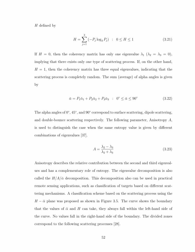
H defined by

H =3∑

j=1

(−Pj log3 Pj) : 0 ≤ H ≤ 1 (3.21)

If H = 0, then the coherency matrix has only one eigenvalue λ1 (λ2 = λ3 = 0),

implying that there exists only one type of scattering process. If, on the other hand,

H = 1, then the coherency matrix has three equal eigenvalues, indicating that the

scattering process is completely random. The sum (average) of alpha angles is given

by

α = P1α1 + P2α2 + P3α3 : 0◦ ≤ α ≤ 90◦ (3.22)

The alpha angles of 0◦, 45◦, and 90◦ correspond to surface scattering, dipole scattering,

and double-bounce scattering respectively. The following parameter, Anisotropy A,

is used to distinguish the case when the same entropy value is given by different

combinations of eigenvalues [37].

A =λ2 − λ3λ2 + λ3

(3.23)

Anisotropy describes the relative contribution between the second and third eigenval-

ues and has a complementary role of entropy. The eigenvalue decomposition is also

called the H/A/α decomposition. This decomposition also can be used in practical

remote sensing applications, such as classification of targets based on different scat-

tering mechanisms. A classification scheme based on the scattering process using the

H − α plane was proposed as shown in Figure 3.5. The curve shows the boundary

that the values of α and H can take, they always fall within the left-hand side of

the curve. No values fall in the right-hand side of the boundary. The divided zones

correspond to the following scattering processes [28].

52

Figure 3.5: Feasible region in H− α plane for random media scattering problems [28].

• Zone 9: Low Entropy Surface Scatter

In this zone, relatively homogenious surface scattering, which do not involve

180◦ phase inversions between HH and VV, such as scattering from water sur-

face, sea ice as well as land surface, dominates the scattering process. Note also

that system measurement noise from very smooth surfaces will act to increase

the entropy and so the system noise floor should also be taken into account

when to set the boundary.

• Zone 8: Low Entropy Dipole Scattering

Dipole scattering from sparse vegetation and non-isotropic scatterers with large

amplitude difference between HH and VV polarizations occurs in this zone.

• Zone 7: Low Entropy Multiple Scattering Events

Low entropy double- or even-bounce scattering events occur in this zone, arising

from isolated dielectric and metallic dihedral scatterers like buildings and man-

made structures.

• Zone 6: Medium Entropy Surface Scatter

In this zone, the additional secondary scattering is caused by increased surface

roughness and microwave penetration into vegetation, leading to the increase

53

in entropy.

• Zone 5: Medium Entropy Vegetation Scattering

Scattering from vegetation surfaces with anisotropic scatterers and moderate

correlation of scatterer orientations occurs in this zone.

• Zone 4: Medium Entropy Multiple Scattering

This zone accounts for dihedral scattering with moderate entropy. For example,

double-bounce mechanisms between the ground and and tree trunks passing

through a cloud of branches, and also urban areas of many scattering centers.

• Zone 3: High Entropy Surface Scatter

This zone is not within the feasible region in the H − α plane. The surface

scattering cannot be identified when H > 0.9. This is a direct consequence of

our increasing inability to classify scattering types with increasing entropy.

• Zone 2: High Entropy Vegetation Scattering

Scattering from forest canopies and vegetation with randomly oriented anisotropic

scatterers lie in this region.

• Zone 1: High Entropy Multiple Scattering

Double bounce mechanisms in a high entropy environment can be categorized in

this region. This mainly occurs in forests and tall vegetation with well developed

branches and crown structures.

From the results, it can be said that the H − α analysis is a useful technique

to distinguish different scattering mechanisms, such as those from forest, water or

urban areas. However, in [28], the boundaries separating zones are arbitrarily chosen,

and are not necessarily accurate. There are some strategies to improve classification

results. One is to introduce the “fuzzy” logic to the boundaries [38] and another is

54

to use image classifiers. Many image classifiers for PolSAR have been proposed and

most of them are based on the feature vector in feature space, including the maximum

likelyhood and minimum distance classifiers. They are already extensively used in

image processing of optical remote sensing data. A classifier known as the Whishart

classifier has also been proposed as a promising tool, utilizing the coherency matrix

which is said to obey the Whishart distribution [39, 40].

55

Chapter 4

4-CSPD Algorithm with Rotation

of Covariance Matrix

The present study introduces the 4-CSPD algorithm with rotation of covariance ma-

trix, and presents an experimental proof of the equivalence between the 4-CSPD algo-

rithms based on rotation of covariance matrix and coherency matrix. Theoretically,

the 4-CSPD algorithms with rotation of the two matrices are identical. Although

it seems obvious, no experimental evidence has yet been presented. In this study,

using PolSAR data acquired by ALOS-PALSAR, an experimental proof is presented

to show that both algorithms indeed produce identical results.

An obscure point in the previous publications was also made clear. That is, there

is ambiguity in minimizing the cross-polarized term in order to enhance the double-

bounce scattering component by rotation of polarimetric matrices.

56

4.1 Overview

With increased quality of SAR systems utilizing polarimetric information recently, the

development and applications of PolSAR are one of the current major topics in radar

remote sensing. While conventional SAR systems handle only single polarimetric

information, data acquired through PolSAR systems contain fully polarimetric infor-

mation on the shift in polarization between the transmitted and received microwave.

Thus, they have potential to increase further the ability of extracting physical quan-

tities of the scattering targets. Therefore, they are used in broad fields of study such

as land cover classification [14, 28, 36, 41], visualization for classification [21, 22], oil

slick detection [23, 24], and ship detection [25, 26], to name a few.

Several decomposition techniques have been proposed along with the utilization

of fully polarimetric data sets provided by PolSAR platforms. Most of them can

be categorized into either of two main groups. One is based on eigenvalue analysis

[11, 13, 28], and the other employs scattering model-based decomposition originally

proposed by Freeman and Durden [14]. The basic idea behind the latter is that the

backscattering power can be expressed as a linear sum of three different scattering

power components.

The 4-CSPD [36, 41] is one of the model-based decomposition methods, and it is an

improved method of the previously devised three-component decomposition [14]. Us-

ing the 4-CSPD, one can decompose PolSAR data into four power categories: surface

scattering power, double-bounce scattering power, volume scattering power, and helix

scattering power. Many studies are being made in this field. For example, Zhang et

al. [42] suggested a multiple-component scattering model (MCSM) by introducing an

additional component that they call wire scattering. Some other studies incorporate

an eigenvalue analysis into model-based decomposition [43, 44, 45] to correct for neg-

57

ative eigenvalues from the remainder covariance matrix after the volume contribution

is subtracted.

According to [11, 12, 14], among all of the scattering components, double-bounce

scattering occurs when the transmitted signal is reflected by ground/sea surfaces and

man-made structures (or natural targets such as tree trunks). However, the prob-

lem appears for oblique urban blocks or man-made structures whose main scattering

center is at an oblique direction with respect to the radar illumination [46]. In such

areas, volume scattering (the cross-polarized component) often becomes a major scat-

tering process. Thus, output results from the decomposition analysis are sometimes

confusing when classification such as urban and forested areas is made, because vol-

ume scattering comes from both areas. This makes the classification of man-made

structures from other areas difficult. From the classification point of view, these two

types of areas have quite different characteristics. Therefore, it would be better if

these areas are separated more clearly.

To overcome this problem, the concept of rotation in the 4-CSPD has recently been

proposed by Yamaguchi et al. [46]. They applied rotation to coherency matrices, so

that the cross-polarization (i.e., HV and VH) components, which are directly related

to volume scattering, are suppressed, and double-bounce scattering increases instead.

As a result, urban or industrial areas are successfully separated from forested areas

more effectively. A rotation angle where the derivative of the rotated cross-polarized

term in a rotated coherency matrix becomes zero is to be chosen for suppressing the

cross-polarized components. However, this explanation leaves ambiguity since the

derivative can be zero when the rotated cross-polarized term is either local maximum

or local minimum (extreme values). Thus, this ambiguity needs to be resolved to

ensure that the cross-polarized term is truly minimum.

In the present article, we introduce the 4-CSPD algorithm with rotation of covari-

58

ance matrix and compare rotation of coherency and covariance matrices. This is

because, although both approaches should yield a same result [47], detailed compar-

ison has not yet been made and reported to date. Comparison is made among the

4-CSPD analyses with and without rotation of matrices. Experimental results are

presented using ALOS-PALSAR PLR (PoLaRimetric) data.

4.2 Rotation of Covariance Matrix

Since the detail of rotation of coherency matrix can be found in [46], we describe

only rotation of covariance matrix, which should give the same results to the rotation

of covariance matrix (although experimental verification has not yet been reported).

The covariance matrix can be expressed as:

⟨[C]⟩ =

⟨|SHH |2⟩ ⟨

√2SHHS

∗HV ⟩ ⟨SHHS

∗V V ⟩

⟨√2SHV S

∗HH⟩ ⟨2|SHV |2⟩ ⟨

√2SHV S

∗V V ⟩

⟨SV V S∗HH⟩ ⟨

√2SV V S

∗HV ⟩ ⟨|SV V |2⟩

=

C11 C12 C13

C21 C22 C23

C31 C32 C33

(4.1)

where SHH , SHV , SV H and SV V denote the complex scattering elements at HH, HV,

VH, and VV polarizations respectively, ⟨⟩ denotes the ensemble average of an arbitrary

window size, and ∗ denotes complex conjugate. The covariance matrix after rotation

can be expressed using a unitary rotation matrix as:

[C(θ)] = [Uθ][C][Uθ]T (4.2)

59

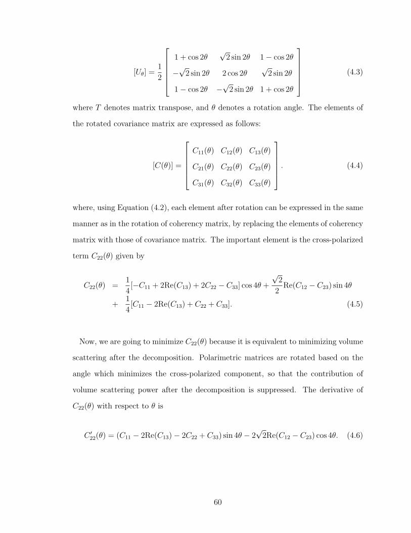
[Uθ] =1

2

1 + cos 2θ

√2 sin 2θ 1− cos 2θ

−√2 sin 2θ 2 cos 2θ

√2 sin 2θ

1− cos 2θ −√2 sin 2θ 1 + cos 2θ

(4.3)

where T denotes matrix transpose, and θ denotes a rotation angle. The elements of

the rotated covariance matrix are expressed as follows:

[C(θ)] =

C11(θ) C12(θ) C13(θ)

C21(θ) C22(θ) C23(θ)

C31(θ) C32(θ) C33(θ)

. (4.4)

where, using Equation (4.2), each element after rotation can be expressed in the same

manner as in the rotation of coherency matrix, by replacing the elements of coherency

matrix with those of covariance matrix. The important element is the cross-polarized

term C22(θ) given by

C22(θ) =1

4[−C11 + 2Re(C13) + 2C22 − C33] cos 4θ +

√2

2Re(C12 − C23) sin 4θ

+1

4[C11 − 2Re(C13) + C22 + C33]. (4.5)

Now, we are going to minimize C22(θ) because it is equivalent to minimizing volume

scattering after the decomposition. Polarimetric matrices are rotated based on the

angle which minimizes the cross-polarized component, so that the contribution of

volume scattering power after the decomposition is suppressed. The derivative of

C22(θ) with respect to θ is

C ′22(θ) = (C11 − 2Re(C13)− 2C22 + C33) sin 4θ − 2

√2Re(C12 − C23) cos 4θ. (4.6)

60

Therefore, when C ′22(θ) = 0, the angle is

tan 4θ =2√2Re(C12 − C23)

C11 − 2Re(C13)− 2C22 + C33

. (4.7)

θ =1

4tan−1 2

√2Re(C12 − C23)

C11 − 2Re(C13)− 2C22 + C33

. (4.8)

An extreme value can be derived from applying Equation (4.8) to Equation (4.5).

However, the obtained extreme value can be either local maximum or local mini-

mum. According to standard mathematical definition, arctangent returns an angle

associated with an extreme value only within a range of (-π/2, π/2], and thus, the

rotation angle range of (4.8) is within (-π/8, π/8]. Since a period of (4.5) is π/2, only

one extreme value is derived from (4.5), and therefore, there is no guarantee that

the calculated extreme value is local minimum required for minimizing the volume

scattering component.

This problem can be fixed by modifying the angle derived from (4.8) as follows:

θmin =

θ (if C22(θ) is local minimum)

θ ± π/4 (otherwise)

(4.9)

where θmin is the angle which surely minimizes the cross-polarized component in C(θ).

We call this modification the modified differential approach.

It should also clearly be stated that many programming languages have an arctan2

function which returns an angle within a range of (-π, π]. Although it is still unclear

whether the calculated value from arctan2 function is local maximum or local min-

imum, it is experimentally shown that arctan2 function returns an angle associated

with local minimum of C22(θ).

61

A local minimum can also be calculated by a brute-force approach. This approach

can be implemented more easily than the derivative method, but at the expense

of slightly increased computation time, by simply changing the angle gradually and

calculate C22(θ) value for each angle across a range of (-π/4, π/4]. From the location

of minimum C22, the corresponding angle θ can readily be found. The brute-force

approach can be used to verify the correctness of the modified differential approach.

4.3 4-CSPD Algorithm Using Rotated Covariance

Matrix

The algorithm of the 4-CSPD analysis using rotation of covariance matrix is sum-

marized in this section. Figure 4.1 is the flowchart of the entire algorithm. First,

rotated covariance matrix [C(θ)] is created using the rotation angle described in the

previous section. Next, the 4-CSPD algorithm is applied to the rotated covariance

matrix [C(θ)] and the scattering powers are calculated. The helix scattering power

Pc is derived first. Then, the volume scattering power Pv is calculated based on the

value of

10 log10[C33(θ)/C11(θ)] (4.10)

Once Pc and Pv are calculated, the surface scattering power Ps and the double-

scattering power Pd can be determined by the remaining power (TP − Pc − Pv). If

Pv+Pc > TP , the algorithm ends as two-component scattering power decomposition.

The branch condition Re(C0) > 0 is used for determining which scattering power, Ps

or Pd, is dominant. C0 can be defined in terms of the covariance matrix elements as:

C0 = C13(θ)−1

2C22(θ) +

1

2Pc. (4.11)

62

Figure 4.1: 4-CSPD algorithm using rotation of covariance matrix (the structure ofentire flowchart mainly comes from [46]).

63

As a result, all of the four scattering components are determined. If Ps or Pd

becomes negative, it is substituted by zero and the other is determined by TP−Pc−Pv.

It should also be noted that all of the four scattering components can be obtained

directly from the rotated covariance matrix elements.

Since covariance matrix and coherency matrix are mutually interchangeable by

unitary transformation, the output of this algorithm should exactly be the same as

the output from the rotation of coherency matrix as long as the same angle, the one

which optimally minimizes the cross-polarized component, is chosen. This can easily

be proven mathematically that both Equation (4.8) and

2θ =1

2tan−1 2Re(T23)

T22 − T23. (4.12)

from [46] have exactly the same form by assigning relevant scattering components into

each equation. As for the equivalence between covariance and coherency matrix, it

can also be shown mathematically that Pc and Pv have exactly the same form in both

algorithms (covariance and coherency matrices) using the same manner as above.

Thus, their equivalence is guaranteed. This equivalence applies to Equation (4.10)

and Equation (4.11) as well. The contribution of the remaining components, Ps and

Pd, should also be identical in both matrices as stated in [47]. In order to confirm

the equivalent nature between the 4-CSPD based on the covariance and coherence

matrices, we provide the experimental results by both approaches in the following

section.

64

4.4 Experimental Results and Discussions

The algorithm is applied to ALOS-PALSAR data, and the results and discussions

are presented in this section. Figure 4.2 shows parts of decomposed images of the

Tokyo Bay and Futtsu Horn in Chiba Prefecture, Japan. The central coordinate is

approximately at (139◦52’E, 35◦20’N), and the image size is approximately 11 km

in both directions. The quad-polarization data used here were acquired by ALOS-

PALSAR on 24 November 2008 (ALPSRP150972900-P1.1). In Figure 4.2, the left

column shows the results from coherency matrix and the right column shows the re-

sults from covariance matrix. The upper row shows the decomposition images from

conventional 4-CSPD and the lower row shows the decomposition images from 4-

CSPD with rotation. The red, green, and blue colors represent the double-bounce,

volume, and surface scattering components respectively. We confirmed that the dif-

ference is zero between the image from covariance matrix rotation and the image

from coherency matrix rotation, as well as those without rotation. This result verifies

that the rotation algorithm with covariance matrix agrees with the theoretical fact of

unitary transformation.

The effect of the size of the moving window for taking ensemble average has also

been analyzed. As expected, if the size is too small, the result is too noisy and

classification does not work very well. On the other hand, if the size is too large,

the output becomes rougher and fine details are lost. An appropriate window size

depends on each situation. Therefore, when the decomposition is performed, this

should be taken into consideration. At this time, the ensemble average window size

is 2 pixels in range direction and 16 pixels in azimuth direction.

Table 4.1 shows comparison of relative contribution of double-bounce, volume, sur-

face, and helix scatterings to the total power before and after rotation, using the same

65

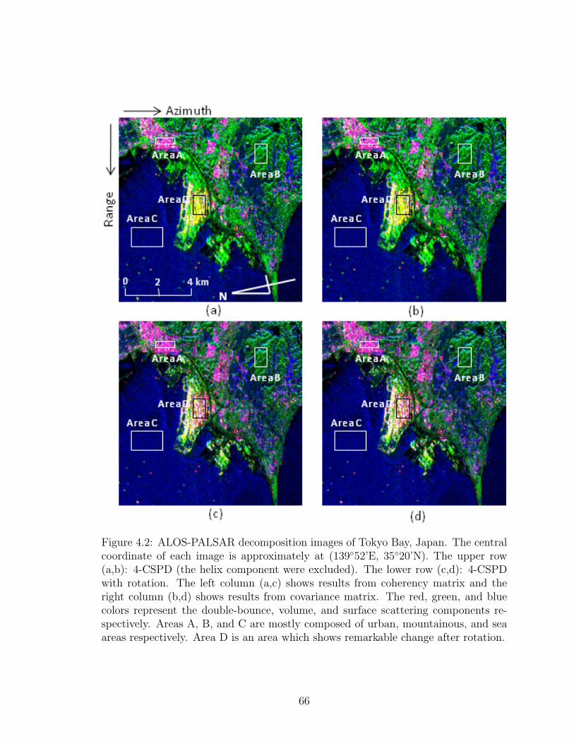
Figure 4.2: ALOS-PALSAR decomposition images of Tokyo Bay, Japan. The centralcoordinate of each image is approximately at (139◦52’E, 35◦20’N). The upper row(a,b): 4-CSPD (the helix component were excluded). The lower row (c,d): 4-CSPDwith rotation. The left column (a,c) shows results from coherency matrix and theright column (b,d) shows results from covariance matrix. The red, green, and bluecolors represent the double-bounce, volume, and surface scattering components re-spectively. Areas A, B, and C are mostly composed of urban, mountainous, and seaareas respectively. Area D is an area which shows remarkable change after rotation.

66

Table 4.1: Relative contribution to total power of Tokyo Bay area before and afterrotation.

Method Pd Pv Ps Pc

4-CSPD without rotation (Area A) 76.64% 2.03% 20.88% 0.45%4-CSPD with rotation (Area A) 76.87% 1.69% 21.06% 0.37%4-CSPD without rotation (Area B) 3.50% 71.35% 19.53% 5.62%4-CSPD with rotation (Area B) 9.39% 57.85% 27.40% 5.57%4-CSPD without rotation (Area C) 0.92% 9.02% 89.33% 0.73%4-CSPD with rotation (Area C) 1.17% 8.21% 89.89% 0.73%4-CSPD without rotation (Area D) 43.63% 46.48% 6.81% 3.09%4-CSPD with rotation (Area D) 81.54% 5.67% 11.63% 1.16%

region as in Figure 4.2. Only results from 4-CSPD with rotation of covariance matrix

are shown in Table 4.1 because we confirmed that the results are precisely identi-

cal between coherency and covariance matrices. After rotation, volume scattering is

suppressed and the contribution of double-bounce scattering becomes larger.

The central area in Figure 4.2 are classified as yellow in the upper images, but are

classified as red in the lower images, increasing likelihood of being recognized as man-

made structures. Figure 4.3 is an enlarged Google Earth image corresponding to the

area in Figure 4.2. The red areas in the lower images in Figure 4.2 can be identified

as industrialized bay areas in Figure 4.3, and the surface scattering areas represented

in blue over land correspond to the rice paddies. After harvest in autumn these

paddy fields are left as rough surfaces of bare soil. Some of the dots scattered on the

sea surface turned into reddish from greenish after rotation and they are considered

to be ships because they show strong Pd scattering and we know that there are no

small islands in the area. Thus, the rotation method helps, by emphasizing the Pd

component, to classify backscattering on the sea not as rocks or tiny islands but as

ships with more certainty.

Figure 4.4 shows rotation angle distribution of the selected areas in Figure 4.2.

From left to right, the results from Areas A, B, C and D are shown. Area A is

67

Figure 4.3: Optical photograph of the image corresponding to the area in Figure 4.2.The central coordinate of the image is approximately at (139◦52’E, 35◦20’N).

a part of urban area and shows strong double-bounce scattering before applying

rotation. Small rotation is observed in Area A. The possible explanation for this is

that most urban structures are ideally facing the radar in a way that the double-

bounce scattering is mostly observed. Thus, rotation is less necessary here. Area B is

a part of mountainous area covered by forests and shows strong volume scattering. In

Area B, rotation is randomly distributed across the entire range. Because the phases

of the cross-polarized component are randomly distributed, angles minimizing them

are also randomly distributed. Area C is a part of sea area and mostly shows surface

scattering. In Areas A and C, the center of rotation angle distribution is around

zero. Finally, Area D is a part of industrial area which shows remarkable change after

rotation. Here, the peak of angle shifts is around –10◦, which is clearly different from

other areas. It coincides with the fact that the structures in Area D are slightly tilted

to the right as can be seen in Figure 4.3.

68

Figure 4.4: Rotation Angle distribution of the selected areas in Figure 4.2. Horizontalaxis is rotation angle and vertical axis is frequency. (a) Area A. (b) Area B. (c) AreaC. (d) Area D.

Figure 4.5 shows Tokyo Bay Aqua-Line (A highway across Tokyo Bay). The green

color produced by the highway bridge in the left image turned into reddish in the

middle image, highlighting enhanced double-bounce scattering, and Figure 4.5(c)

clearly shows increase in double-bounce scattering between Figure 4.5(a,b). As a

ground truth, we confirmed that the bridge does not have tall towers and large cables

as described in the bridge analysis in [48] and there are many highway lamps and

traffic and direction signs on the bridge. Thus, double-bounce scattering comes from

the dihedral reflection between the surface of the bridge and the highway lamps,

traffic, and direction signs, and also between the sea surface and the bridge. Figure

4.6 shows a rotation angle image and rotation angle distribution around the bridge.

The peak around 30◦ in Figure 4.6(b) corresponds to the direction of the bridge from

the radar illumination.

69

Figure 4.5: Tokyo Bay Aqua-Line (Highway) near the area of Figure 4.2. The cen-tral coordinate of each image is approximately at (139◦53’E, 35◦26’N). (a) 4-CSPDimage without rotation. (b) 4-CSPD image with rotation. (c) Difference of the Pd

component between the left and the middle image.

Figure 4.6: Tokyo Bay Aqua-Line (Highway) near the area of Figure 4.2. (a) Rotationangle image. The central coordinate of the image is approximately at (139◦53’E,35◦27’N). (b) Rotation angle distribution of the left image. The peak around 30degree represents the highway bridge.

70

Chapter 5

Comparison between Eigenvalue

Analyses of Different Polarization

This study clarifies the difference in eigenvalue analysis between quad-, HH/VV dual-,

and HH/HV dual-polarization SAR data. There are different types of data acquisition

modes in SAR systems and each of them has different advantages and disadvantages.

The main advantage of quad-polarisation data is more detailed information about

scattering objects, and those of dual- or single-polarisation data are higher spatial

resolution, wider area coverage, and abundance of available data sets. Thus, there is a

certain trade-off between the SAR data of these acquisition modes, and in the present

study, we focused on the potential information contained in the dual-polarisation data

using the Advanced Land Observation Satellite-Phased Array L-band SAR (ALOS-

PALSAR) quad-polarisation data of the Tokyo Bay, Japan. It was found that the

HH/VV dual-polarization data can produce very close entropy/alpha results to quad-

polarization data while only entropy is reliable in HH/HV dual-polarization data.

71

5.1 Introduction

In the early days, most SAR systems operated with single-polarization. However,

recent technological advancements allowed the development and operation of SAR

systems with multi-polarization observation capability. Quad-polarization data (also

called as fully polarimetric data) have most abundant information on observed targets

compared with single- or dual-polarization data and there are also plentiful analytical

methods for quad-polarization data such as eigenvalue analysis [28] and model-based

decomposition [11, 14].

On the other hand, the richness of quad-polarization data comes at the expense

of spatial resolution and swath widths [49, 50]. There is a certain trade-off relation

between quad- and single-polarization data. Although there are many spaceborne

SAR systems capable of quad-polarization observation, most of them are operated

mainly in single- or dual-polarization mode because of these reasons.

Dual-polarization data may not be as rich in information on targets as quad-

polarization data, but their spatial resolution is higher and swath widths are larger

than those of quad-polarization data. Further, we can perform polarimetric analy-

ses with dual-polarization data utilizing correlation between the two channels that

cannot be applied on single-polarization data, which basically rely on the amplitude

magnitude of the signal. In this study, we examine the information content of dual-

polarization data in entropy/alpha decomposition analysis using ALOS-PALSAR

data by comparing the results with those of quad-polarization data.

The composition of the study is as follows. In Section 5.2, the methodology is sum-

marized, introducing the entropy/alpha decomposition analysis based on HH/VV

dual-polarization data. In Sections 5.3, the ALOS-PALSAR data of the Tokyo Bay,

Japan are described, followed by results and conclusions in Sections 5.4 and 5.5 re-

72

spectively. For simplicity, we, hereafter, term the alpha/entropy decomposition using

dual- and quad-polarization data as dual and quad alpha/entropy decomposition,

respectively.

5.2 Methodology

We consider two types of dual-polarization combination, HH/VV and HH/HV. HH/VV

dual-polarization data do not have all the advantages stated in Section 1, and that

is why studies on HH/VV dual-polarization is significantly fewer than studies on

HH/HV dual-polarization. However, HH/VV dual-polarization data contain infor-

mation close to quad-polarization data and some spaceborne SAR such as ENVISAT-

ASAR and TerraSAR-X have HH/VV data acquisition mode. The advantage of this

mode is that less data transfer bandwidth is necessary compared with quad aquisi-

tion mode. Also, if we can approximate quad eigenvalue analysis with dual eigenvalue

analysis, we can take advantage of faster computational time that is required for real-

time systems or applications at the expense of rigorously accurate results.

There are a substantial number of studies to compare dual-polarization data with

quad-polarization data, especially for classification purposes. These studies utilize

complex or amplitude data of each polarization channel [51, 52, 53, 54], but not much

attention has been paid to the comparison of dual- and quad-polarization data using

polarimetric parameters that can be derived from these polarimetric data sets.

Recently, another technique called hybrid polarization is suggested [52, 55]. In this

mode, either circularly polarized signals or signals which are 45◦ slanted to horizon-

tal/vertical axis are transmitted and horizontal/vertical signals are received. The

main advantage of the hybrid polarization is that it requires only one transmission

73

antenna. Also some approximation techniques have been suggested to use eigenvalue

analysis or model-based decomposition with hybrid polarization data [56, 57, 58].

However, we have a large amount of available archives recorded as dual-polarization

SAR data. They are invaluable resources that can be used as huge reference data for

future studies and explorations.

Entropy/alpha decomposition [28] was originally proposed for quad-polarization

data, but modified and applied to dual-polarization data later [59, 60]. The en-

tropy/alpha decomposition algorithm for HH/HV dual-polarisation data can be found

in [59, 61], and the entropy/alpha decomposition algorithm for HH/VV dual-polarisation

data can be expressed as follows:

⟨[T2]⟩ = [U ]

λ1 0

0 λ2

[U ]∗T = λ1u1u∗T1 + λ2u2u

∗T2 (5.1)

[U ] =

U11 U12

U21 U22

=

[u1 u2

](5.2)

ui =

[cosαi sinαie

jδi

]T(5.3)

where ⟨[T2]⟩ is the averaged 2× 2 coherency matrix, λ1 ≥ λ2 are the eigenvalues, U is

the orthogonal unitary matrix, and δi is the relative phase difference.∗ and T denote

the complex conjugate and transpose, respectively. Entropy H and alpha angle α can

be expressed as

H = −P1 log2 P1 − P2 log2 P2 (5.4)

α = P1 cos−1(|U11|) + P2 cos

−1(|U12|) (5.5)

where

Pi =λi

λ1 + λ2. (5.6)

74

5.3 Polarimetric SAR Data

The ALOS-PALSAR quad-polarization data used in this study were acquired on 24

November 2008 over Tokyo Bay, Japan with descending mode and an off-nadir angle

of 21.5◦ (Scene ID: ALPSRP150972900-P1.1). The resolution is 20 m in azimuth

direction and between 24 m and 33 m in range direction depending on incidence

angle. The sample pixel size is 3.56 m in azimuth and 9.37 m in range direction.

Figure 5.1 shows the original HH, VV, and HV polarization images. The image

center is approximately at 139◦48’E, 35◦17’N, and the image size is approximately 25

km in both azimuth and range directions. The land on the bottom-left in the images

is predominantly covered with residential houses, markets and hills with trees. In

the Tokyo Bay, one of the busiest ports in Japan, many ships of different sizes can

be seen. At the time of the data acquisition, there was underwater laver (seaweed)

cultivation around the pointed peninsula, Cape Futtsu, in the center of the image.

On the right-hand side, there are industrial and urban areas up north with some

residential houses along the coast, and the rest of the land is mostly forests on hills

or flatland.

5.4 Experimental Results and Discussions

Figure 5.2 is a comparison between quad and dual entropy/alpha decomposition and

Figure 5.3 shows the comparison of selected individual areas of sea surface, buildings,

and forests as indicated by the labeled (”a” to ”r”) squares in Figure 5.2. The visual

inspection of the entropy and alpha angle images in Figure 5.2 and 5.3 shows close

similarity between the results based on the quad- and HH/VV dual-polarization data,

whereas the results from HH/HV dual-polarization data are considerably different

75

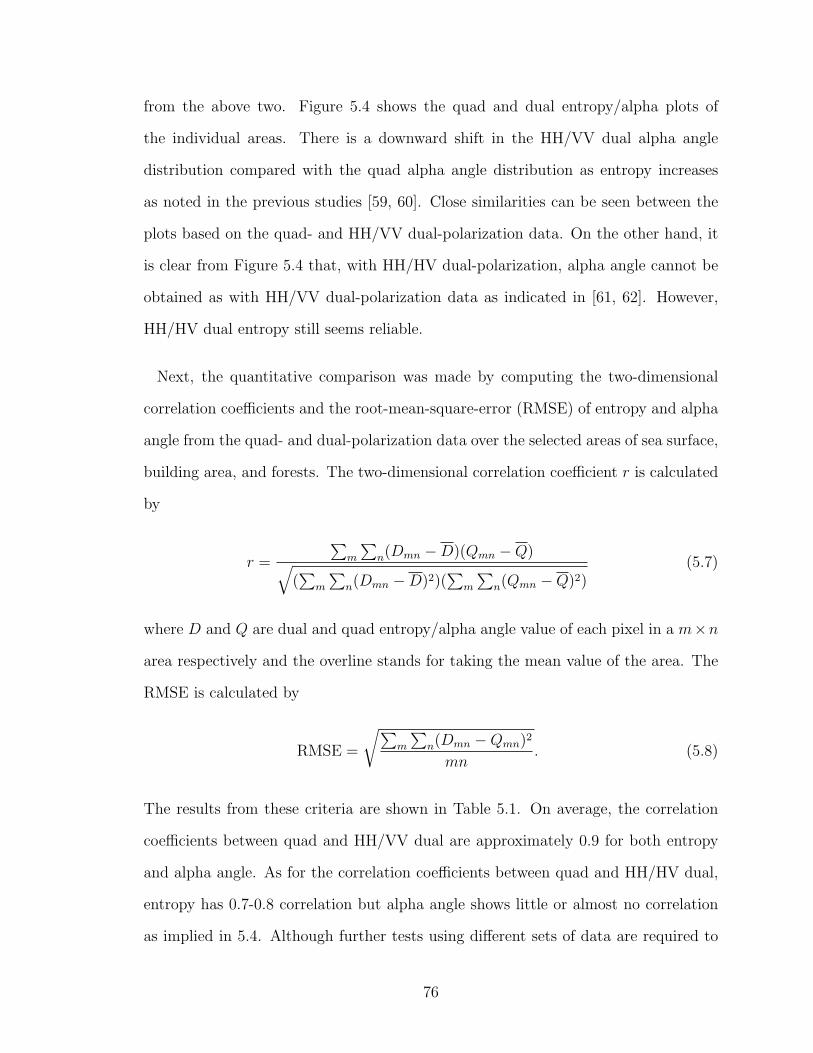
from the above two. Figure 5.4 shows the quad and dual entropy/alpha plots of

the individual areas. There is a downward shift in the HH/VV dual alpha angle

distribution compared with the quad alpha angle distribution as entropy increases

as noted in the previous studies [59, 60]. Close similarities can be seen between the

plots based on the quad- and HH/VV dual-polarization data. On the other hand, it

is clear from Figure 5.4 that, with HH/HV dual-polarization, alpha angle cannot be

obtained as with HH/VV dual-polarization data as indicated in [61, 62]. However,

HH/HV dual entropy still seems reliable.

Next, the quantitative comparison was made by computing the two-dimensional

correlation coefficients and the root-mean-square-error (RMSE) of entropy and alpha

angle from the quad- and dual-polarization data over the selected areas of sea surface,

building area, and forests. The two-dimensional correlation coefficient r is calculated

by

r =

∑m

∑n(Dmn −D)(Qmn −Q)√

(∑

m

∑n(Dmn −D)2)(

∑m

∑n(Qmn −Q)2)

(5.7)

where D and Q are dual and quad entropy/alpha angle value of each pixel in a m×n

area respectively and the overline stands for taking the mean value of the area. The

RMSE is calculated by

RMSE =

√∑m

∑n(Dmn −Qmn)2

mn. (5.8)

The results from these criteria are shown in Table 5.1. On average, the correlation

coefficients between quad and HH/VV dual are approximately 0.9 for both entropy

and alpha angle. As for the correlation coefficients between quad and HH/HV dual,

entropy has 0.7-0.8 correlation but alpha angle shows little or almost no correlation

as implied in 5.4. Although further tests using different sets of data are required to

76

validate the equivalence, the preliminary results of this study have shown that the

entropy/alpha decomposition analysis with HH/VV polarization combination is as

practical as the entropy/alpha decomposition with quad-polarization data.

Table 5.1: Quantitative evaluation of differences between quad- and HH/VV dual-analysis or between quad- and HH/HV dual-eigenvalue analysis. The values withoutparenthesis are results from quad- and HH/VV dual-eigenvalue analysis and the valuesin parenthesis are results from quad- and HH/HV dual-eigenvalue analysis.

Parameter (area) Correlation coefficient RMSE

Entropy (sea area) 0.9113 (0.7828) 0.0295 (0.0733)

Entropy (vegetation area) 0.8722 (0.7466) 0.0560 (0.1546)

Entropy (urban area) 0.8715 (0.7797) 0.1019 (0.2435)

Alpha angle (sea area) 0.8922 (-0.2253) 0.0354 (0.3483)

Alpha angle (vegetation area) 0.8791 (0.0175) 0.1426 (0.0961)

Alpha angle (urban area) 0.9251 (0.2814) 0.1077 (0.1409)

77

Figure 5.1: The original ALOS-PALSAR quad-polarization amplitude images ac-quired on 24 November 2008 over the Tokyo Bay, Japan. (a) HH polarization image.(b) VV polarization image. (c) HV polarization image.

78

Figure 5.2: Comparison between quad- (upper row), HH/VV dual- (middle row), andHH/HV dual- (lower row) entropy/alpha decomposition. (a) Quad entropy image.(b) Quad alpha angle image. (c) HH/VV dual entropy image. (d) HH/VV dual alphaimage. (e) HH/HV dual entropy image. (f) HH/HV dual alpha image.

79

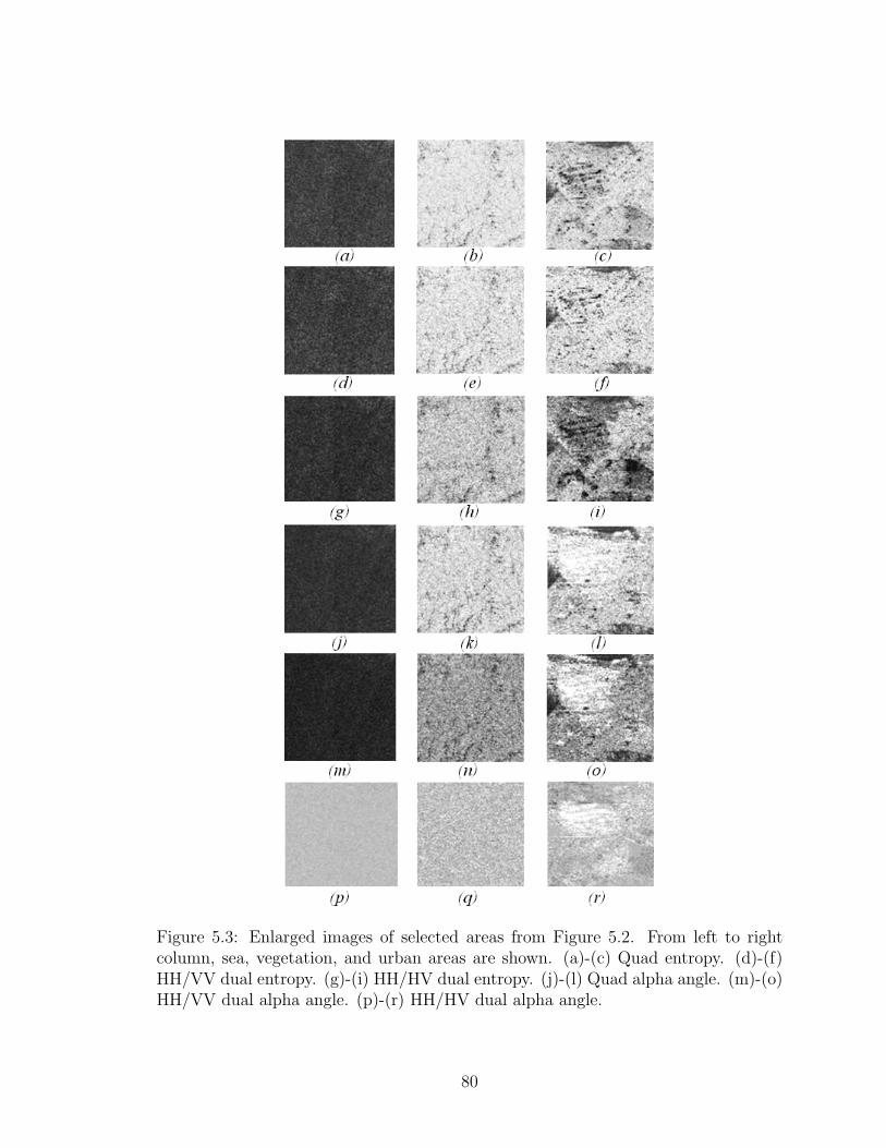
Figure 5.3: Enlarged images of selected areas from Figure 5.2. From left to rightcolumn, sea, vegetation, and urban areas are shown. (a)-(c) Quad entropy. (d)-(f)HH/VV dual entropy. (g)-(i) HH/HV dual entropy. (j)-(l) Quad alpha angle. (m)-(o)HH/VV dual alpha angle. (p)-(r) HH/HV dual alpha angle.

80

Figure 5.4: Entropy/alpha plots of selected areas from quad- (upper row), HH/VVdual- (middle row), and HH/HV dual- (lower row) eigenvalue analyses. From left toright column, sea, vegetation, and urban areas are shown. (a)-(c) Quad entropy/alphaplot. (d)-(f) HH/VV dual entropy/alpha plot. (g)-(i) HH/HV dual entropy/alphaplot.

81

Chapter 6

Marine Target Detection Using the

Model-Based Decomposition

In this study, we show the novel applications of the model-based scattering power

decomposition analyses in SAR polarimetry to man-made target detection on the sea

surface. The model-based decomposition technique is primarily used for land cover

classification mainly because the microwave scattering from land is composed of var-

ious scattering mechanisms, such as surface, double-bounce, and volume scattering.

On the other hand, this technique has not been widely used for oceanic applications

since the scattering from sea is mostly surface scattering, and obtaining a classifica-

tion of different types of scattering is not as important as that on land. However, if

an object is present on the sea surface, which gives rise to different scattering charac-

teristics from the sea surface, the decomposition approach may be a useful technique

for detection and classification of the object. We suggest two approaches for target

detection on the sea surface. One is to use the model-based decomposition as a po-

larimetric band-stop filter to block the dominant scattering from the background sea

surface, and the other is to focus on the optimized double-bounce scattering compo-

82

nent associated with the target using a rotation scheme of the polarimetric matrix.

The advantage of these methods is the simplicity of the concept and algorithm, in

which no target-centric analysis is necessary. Experimental results show that the

model-based decomposition analyses can work as a powerful target detector, effec-

tively separating the scattering by targets from the dominant background scattering

from the sea surface.

6.1 Introduction

Recent technological trends involving SAR are moving toward the utilization of multi-

polarization data. Many attempts have been made to separate intended targets from

the sea using single- or dual-polarization SAR data, and there are excellent studies

utilizing the speckle properties of single-polarization data [63] and different symmetry

properties of the sea and those of the targets [64]. With fully polarimetric data

containing amplitude and relative phase information among different polarimetric

channels, more detailed analyses about the targets are possible.

Many studies that utilizes the model-based decomposition technique focus on land

cover or urban area classification because of their classification capability [41, 42, 43,

44]. In this letter, we show the novel use of the 4-CSPD for detecting targets on

the sea surface. ALOS-PALSAR polarimetric data and available reference data for

validation are used in the study.

The composition of the study is as follows. In Section 6.2, the methodology used in

this study is summarized. In Sections 6.3, the ALOS-PALSAR and ground truth data

of Portsmouth, UK, are described, followed by results and conclusions in Sections 6.4

and 6.5 respectively.

83

Figure 6.1: Scattering from ships.

6.2 Methodology

Scattering from ships, for example, on the sea surface is often more complex than

scattering from the sea surface as illustrated in Figure 6.1. Scattering from such

man-made objects often consists of not only surface scattering but also a considerable

amount of double-bounce and volume scattering. This difference in the scattering

mechanism between the sea surface and man-made objects allows us to detect the

objects using the model-based decomposition analyses.

The fact mentioned above leads to the following idea: if the surface scattering

component is subtracted from the total power (TP ), most of the scattering from

the sea can be excluded, thereby revealing other objects on the sea surface including

ships. We term this approach as TP−Ps. Another idea is to utilize double-bounce

scattering, which is a good indicator of the presence of man-made objects, and can

therefore be used as a man-made object detector. However, the observed intensity of

double-bounce scattering can fluctuate depending on the relative orientation between

the SAR platform and the structures of man-made objects. This often results in

underestimated double-bounce scattering and overestimated volume scattering. To

84

minimize the effect of this phenomenon, a rotation scheme of the polarimetric matrix

is introduced [46, 65].

One certain advantage of these two approaches other than detection capability is

the simplicity of the concept. There is no need for pre-learning process about targets

or detailed target-centric analysis. As a result, volume scattering is minimized and

double-bounce scattering is maximized. The double-bounce scattering component

obtained from the rotation scheme is referred to as the optimized Pd. We use these

two approaches for target detection on the sea.

In addition to its detection ability, one clear advantage of these two approaches

is the simplicity of the concept. There is no need for pre-learning processes about

targets or detailed target-centric analyses.

The detection process is shown in Figure 6.2. First, the 4-CSPD is performed on

fully polarimetric SAR data. The parameters representing the above two approaches

(TP −Ps and optimised Pd) can easily be obtained from the decomposition result.

Land masking is then applied because the adaptive-constant false alarm rate (CFAR)

processing is largely affected by the scattering from the land area [50]. Next, a

background area (a homogeneous sea area where there are no ships or other objects) is

chosen from the images in order to analyze the statistical distribution of the scattering

intensity from the sea surface, and the best fit probability density function (PDF)

is chosen depending on the likelihood criterion. Finally, targets are detected using

the adaptive-CFAR method based on the assumption that the statistical intensity

distribution of each local area is the same as the chosen PDF from the selected

homogeneous background area, and a threshold value is determined for each local

region.

85

Figure 6.2: Flowchart of detection process.

6.3 PolSAR Data and Ground Truth

The ALOS-PALSAR quad-polarization data used in this study were acquired at 22:03

(UT) on 26 March 2011 over the coast of Portsmouth, UK, in the ascending mode

with the off-nadir angle of 21.5◦ (Granule ID: PASL100110326220622). The process

level is 1.1 and the resolution is 4.89 m in the azimuth direction and 11.09 m in the

slant range direction (approximately 30 m ground range resolution). The sampling

pixel size is 3.55 m in the azimuth direction and 9.37 m in the slant range direction

(approximately 25 m ground range resolution). Figure 6.3 (a) is a Google Map image

of the region around Portsmouth. At the time of the SAR data acquisition, the sea

was at low tide, the average wind speed was approximately 3 m/s with the wind

direction of 80 degrees, and the significant wave height was 0.3 m at approximately

10 km east of the test site.

Figure 6.4 (a)–(c) shows HH, VV and HV amplitude images, respectively, and

Figure 6.4 (d) shows the decomposed image of the test site. The white rectangle is

86

Figure 6.3: A Google Map image of the area around Portsmouth. The central coor-dinate of the image is approximately at 50◦45’N, 1◦04’W. The white rectangle at thecenter of the image represents the test site analyzed in this study. Imagery c⃝2012TerraMetrics. Map data c⃝2012 Google (accessed November 6, 2012).

an area chosen as the homogeneous background area for the PDF estimation. The

ensemble window size for the decomposition algorithm is chosen as 1 pixel in the

range direction and 7 pixels in the azimuth direction, corresponding to about 25 ×

25 m per pixel after the decomposition.

Figure 6.5 is the reference data showing the locations of the man-made objects

(buoys and beacons). The buoys are approximately 3 m in height and 3 m in diameter.

The beacons are column-shaped and approximately 2 m in height and 30 cm in

diameter. They are built along with submarine barriers leading from Portsmouth out

to the Spit Sand Fort and the barriers are above the sea surface at low tide (i.e. at

the time of the SAR data acquisition). The Spit Sand Fort and the Horse Sand Fort

are relatively large round-shaped objects that were originally used as sea forts. The

Spit Sand Fort is approximately 50 m and the Horse Sand Fort is 73 m in diameter.

87

Figure 6.4: The ALOS-PALSAR quad-polarization amplitude images and the decom-posed image. The image centre is approximately at 50◦46’N, 1◦04’W and the imagesize is approximately 5 km in both azimuth and range directions. (a) HH image. (b)VV image. (c) HV image. (d) Decomposed image of the test site (red: double-bouncescattering, green: volume scattering, blue: surface scattering). The white rectangleis an area chosen as the homogeneous background area.

88

In all images in Figure 6.4, the two forts are clearly identified and can be excluded

from the intended targets. Some of the beacons can also be recognized in Figure 6.4

(a), (b) and (d), but it is difficult to identify the buoys from these images although

they are larger in size than the beacons. A possible explanation is that the right-angle

structures of the submarine barriers and the beacons result in a larger radar cross

section (RCS) than the buoys of round shape.

HV is known to be a better polarization than other polarizations (HH and VV) [50]

for ship detection because the sea clutter is weak in HV data. However, the scattering

from other targets may also be small in HV, as shown in Figure 6.4 (c), where it is

difficult to distinguish the the beacons from the background sea clutter. From the

intensity distribution of the surface scattering component (the blue area) in Figure

6.4 (d), it can be implied that the sea state is relatively rough on the top left side of

the area and calm in the remaining sea area. Also, no ship was confirmed at the time

of the SAR data acquisition.

6.4 Experimental results and Discussions

Figure 6.6 (a) shows the TP−Ps image (left) and Figure 6.6 (b) describes the statistical

intensity distribution of the background area marked by the rectangle in Figure 6.6

(a) together with the candidate PDFs. Among these PDFs, the gamma distribution

showed the highest similarity to the background distribution of the TP−Ps image.

Figure 6.7 shows the image and the distribution of the optimised Pd, and the best-fit

PDF was the Weibull distribution. Note that Pd may sometimes be zero in the model-

based decomposition, and these zero values are excluded when PDFs are calculated.

A best-fit PDF may vary depending on what component is chosen. The scattering

from the sea, including the rough sea state in the north-west part observed in Figure

89

Figure 6.5: Nautical map as reference data. c⃝Portsmouth Port 2011 (accessedNovember 5, 2012).

6.4 (a), (b) and (d), has been mostly suppressed in Figure 6.6 (a) and Figure 6.7 (a),

since the dominant surface scattering component from the sea surface is removed.

Also, the missing targets (beacons) in Figure 6.4 (c) became visible in Figure 6.6 (a)

and Figure 6.7 (a).

For the adaptive-CFAR processing, each image is divided into sub-images of 20 × 20

pixels, and the false alarm rate (FAR) is set to 1.0 ×10−3 for each TP−Ps sub-image,

and 5.0 × 10−4 for that of the optimised Pd. These FAR values were determined

from the receiver operating characteristic (ROC) curves (Figure 6.8), which show

the relation between true positive rates and false positive rates. The true positive

rates were computed from the number of detected targets divided by the number of

intended targets, and the false positive rates were calculated from the number of false

positive pixels divided by the number of pixels of the whole image, except for the

land-masked area. The two FAR values were selected from the points at which there

90

(a)

0.02 0.04 0.06 0.08 0.1 0.12 0.14 0.16 0.18 0.20

2

4

6

8

10

12

14

16

18

TP - Ps

Density

TP - Ps

Rayleigh

Gamma

Lognormal

Weibull

(b)

Figure 6.6: (a) TP − Ps image. (b) Statistical intensity distribution of backgroundarea marked as rectangles in (a) and candidate PDFs.

(a) (b)

Figure 6.7: (a) Optimized Pd image. (b) Statistical intensity distribution of back-ground area marked as rectangles in (a) and candidate PDFs.

91

Figure 6.8: Receiver operating characteristic (ROC) curves.

is a good trade-off between the true positive rate and the false positive rate (the two

circled points in Figure 6.8).

The detection results by the two approaches are shown in Figure 6.9 and 6.10.

16 out of 17 intended targets were detected from the TP −Ps method, and 15 out

of 17 intended targets were detected from the optimised Pd method. The detection

result from the TP−Ps shows more false positives. It was found that many of these

false positives come from the volume scattering component associated with the calm

sea surface. When the sea is very calm, the backscattering becomes very weak and

comparable to the noise level. In such a case, volume scattering, instead of surface

scattering, often becomes the dominant scattering in the decomposition analyses, due

to the random property of the system noise. Figure 6.8 also clearly shows that the

optimised Pd performs better than the TP−Ps in this experiment, because the former

generally shows a better true positive rate than the latter for a fixed false positive

value as in Figure 6.8.

The same test site and the man-made objects were previously analysed using

92

Figure 6.9: Detection result by TP − Ps (solid circles: detected targets, dashed cir-cles: missed targets).

Figure 6.10: Detection result by optimized Pd (solid circles: detected targets, dashedcircles: missed targets)

93

RADARSAT-2 C-band fully polarimetric SAR data [27]. It was expected that the de-

tection performance with ALOS-PALSAR data would be lower than that of RADARSAT-

2 data because of longer wavelength and coarser spatial resolution. However, our

approach with ALOS-PALSAR data was able to detect most of the targets identified

in the aforementioned study, and it has also been confirmed that with fully polarimet-

ric PALSAR data, smaller targets (approximately 2–3 m) than the PALSAR spatial

resolution can be detected using our approach.

In order to confirm the ability of our approach, we analysed another set of ALOS-

PALSAR data acquired at 01:19 (UT) on October 9th, 2008 over the Tokyo bay,

Japan, and the results are shown in Fig. 6.11. Fig. 6.11 (a) is the decomposed image

of the test site using the 4-CSPD, and dominant surface scattering is observed on the

sea surface. In Fig. 6.11, the rectangles are two sea forts (top) and an island (left).

19 out of 21 ships are visible in the decomposed image. Fig. 6.11 (b) and (c) are the

detection result obtained using the TP−Ps and optimised Pd, respectively, and all of

the ships are detected with TP−Ps after adaptive-CFAR processing. False positives

are effectively inhibited in this sea state (dominant surface scattering).

Comparing the results between Portsmouth and Tokyo bay, we can safely state that

the TP −Ps method is more robust than the Pd method when the scattering from

the sea is strong. This is an interesting property because, in general, ship detection

becomes increasingly difficult as the sea clutter increases. Although it is beyond the

scope of this study and further analysis with appropriate reference data would be

necessary, the optimised Pd should be able to distinguish man-made objects such as

ships from other similar-sized natural targets (rocks/islands) because double-bounce

scattering is mainly unique to artificial targets.

94

(a)

(b)

(c)

Figure 6.11: Ship detection using fully polarimetric ALOS-PALSAR data aroundTokyo bay on 9 October, 2008. The image center is at approximately 35◦17’N,139◦44’E, and the image size is approximately 10 km in range and 7 km in azimuthdirections. Solid circles: visible/detected targets. Dashed circles: invisible/missedtargets. Rectangles: two sea forts (top) and an island (left). (a) Decomposed imageof the test site obtained using the 4-CSPD algorithm (red: double-bounce scattering,green: volume scattering, blue: surface scattering). (b) Detection result obtained byexcluding the surface scattering component. (c) Detection result obtained using theoptimized Pd .

95

Chapter 7

Comprehensive Comparison of

Different Polarimetric Methods

In this study, image contrast between extracted laver cultivation area and background

water was extensively compared using various parameters that can be calculated by

dual- or quad-polarization PolSAR data. Each parameter derived from Pauli de-

composition, eigenvalue analysis, coherence analysis, and four-component scattering

power decomposition (4-CSPD) has distinctive characteristics and react to different

backscatterers differently. Contrast comparison was made using these parameters us-

ing the L-band quad-polarization data acquired by ALOS-PALSAR and the X-band

dual-polarization data acquired by TerraSAR-X, and experimental results showed

that the contrast can be improved using multi-polarization data than using single-

polarization data. It has also been found that entropy performs better among dual-

polarization methods, and the surface scattering component calculated from 4-CSPD

exhibits higher contrast than any other parameters from quad-polarization data.

96

7.1 Introduction

In East Asian countries including China, Japan and Korea, laver cultivation has tra-

ditionally been one of the important marine industries in coastal waters as well as

fishery. Laver (Porphyra) is nutrient-rich food and has been used in many Asian

cuisines. During laver cultivation periods, laver cultivation nets are put on the sea

near the coastlines, and monitoring of the nets is necessary for farming control and

damage assessment occasionally caused by natural disasters such as typhoons and

tsunamis. Laver cultivation is vulnerable to these natural disasters and if these disas-

ters hit laver cultivation area, laver cultivation nets will be devastated and scattered

around the coast. Those devastated structures affect not only nearby residents but

also maritime traffic around the area.

Several studies of laver cultivation monitoring have been made with polarimetric

analysis using ALOS-PALSAR quad-polarization (fully polarimetric) data [66, 67, 68].

One of them is a detailed study of laver cultivation monitoring using polarimetric

entropy [66]. In this study, it was shown that laver cultivation nets can be extracted

using ALOS-PALSAR data utilizing the randomness indicated by entropy on the

images of the underwater laver cultivation nets. However, the comparison of the result

is done only with amplitude data without considering the use of other polarimetric

analyses.

In this study, ALOS-PALSAR quad-polarization data and TerraSAR-X HH/VV

dual-polarization data are used to extract laver cultivation area using the following

methods: Pauli decomposition, eigenvalue analysis [13, 28, 59, 60], coherence analysis

[69], and the four-component scattering power decomposition (4-CSPD) [41]. Then

the results are analyzed and evaluated by comparing contrasts between laver culti-

vation area and background water for parameters derived from these methods. The

97

use of dual-polarization data is also explored for the purpose of extracting the tar-

get area effectively and deciding suitable methods within the limitation of available

polarization.

7.2 Interaction between Laver Cultivation Area and

SAR Microwaves

When laver cultivation nets are placed at approximately 10-20 cm below the sea sur-

face, the area above the nets can be considered as ”shallow water”, and the area

without nets as ”deep water”. Thus, in the cultivation area, Bragg waves, which are

mainly responsible for radar backscatter from the sea surface, are dumped because

of the shallow bottom topography effect. Therefore, the cultivation area should have

smoother sea surface compared with the area without laver cultivation nets (back-

ground water), and this difference in roughness can be appeared in acquired SAR

data. For example, if the surface of cultivation area is smooth enough, the surface

looks as specular surface for SAR, and backscattering from such surface is very small

in each amplitude channel in polarimetric data and close to the system noise level.

Polarimetric entropy should then be high and coherence between HH and VV should

be low in such area because of the randomness of system noise. Although the main

scattering component from the sea should be surface scattering, this extremely low

backscattering from effectively specular surface also affect the alpha angle or surface

scattering component calculated from 4-CSPD. On the other hand, if the nets are

above sea surface, the scattering process will considerably be different because the

cultivation net structures above sea surface will cause complex scattering such as

double-bounce or volume scattering as other man-made structures on land.

98

Figure 7.1: Photograph of a part of the Futtsu Horn test area in Tokyo Bay, Japantaken on 5th of February 2011.

Figure 7.1 shows a photograph of the test site. At the time when this photograph

was taken, the significant waveheight and wind speed were 0.34 m and 3.0 m/s respec-

tively. The very smooth surfaces corresponding to the underwater nets among fairly

rough sea surfaces are clearly visible in the photograph. Note that the photograph of

Figure 7.1 is shown for the purpose of visual illustration on the difference in surface

roughness over the test site, and the date when the photograph was taken is different

from that of PALSAR data acquisition. In the test site of laver cultivation in Tokyo

Bay, Japan, the cultivation nets with attached laver spores are placed underwater in

October, and harvested in the following April in the following year. During the cul-

tivation season, the nets are sometimes placed above water to stimulate and promote

photosynthesis. Among ten sets of available PALSAR quad-polarization data over the

test site, six sets were out of season, and no cultivation nets were observed. two sets

of data showed the nets above water, and in the rest of 2 sets of data the cultivation

nets were underwater. No photograph was taken simultaneously with these SAR data

acquisition days that are prior to the present project, but the weather condition was

similar between these dates.

99

Figure 7.2: The ALOS-PALSAR quad-polarization amplitude images acquired on24 November 2008 over Tokyo Bay, Japan. (a) HH polarization image. (b) VVpolarization image. (c) HV polarization image.

7.3 Experimental results and Discussions

First, experiments were performed using ALOS-PALSAR quad-polarization data.

The quad-polarization data used here were acquired at 9:58 pm (local time) on Octo-

ber 7, 2006 with off nadir angle 21.5◦, and at 10:20 am (local time) on November 24,

2008 with off nadir angle 21.5◦. Figure 7.2 shows HH, VV, and HV amplitude images

of the 2008 data. The image size is approximately 10 km in both (azimuth and range)

directions and the image center is approximately at (35◦17′N, 139◦48′E) where the

cultivation area of interest is located in the coastal waters around the Futtsu Horn

in Tokyo Bay, Japan. Resolution is 20 m in azimuth direction and it ranges from 24

m to 33 m in near-range to far-range directions. The sampled pixel size is 3.56 m in

azimuth and 9.37 m in range direction. The upper and lower rectangles in each image

are used as laver cultivation area and background area respectively.

The process of extracting the cultivation area is as follows. First, median filtering is

applied to the laver cultivation area (upper rectangle in Figure 7.2) in order to reduce

the effect of speckle noise inherent in SAR data. Then, a mask image is created

100

by applying thresholding and morphological filtering to the filtered image. Those

processes are necessary for further reducing the effect of noise, and extracting the

laver cultivation area accurately. Otherwise, the extracted area would contain pixels

corresponding to speckle noise. After that, by interleaving the obtained mask image

and the original image, cultivation area is extracted. Note that although the mask

image is created using median filtering, the extracted cultivation area itself is not

processed by median filtering.

In order to assess the contrast between the extracted cultivation area and back-

ground area in each image, the following criterion, mean contrast, was defined. The

mean contrast is expressed as

Cmean = | ⟨Acultivation⟩ − ⟨Abackground⟩⟨Acultivation⟩+ ⟨Abackground⟩

| (7.1)

where ⟨Acultivation⟩ represents a mean value of pixels in the laver cultivation area and

⟨Abackground⟩ stands for a mean value of pixels in the background area. The values of

Cmean in Figure 7.2 are the mean contrast values for each amplitude image.

At the time of data acquisition, significant wave height was 0.24 m and wind speed

was 2.0 m/s in 2006 data and these were 0.6 m and 2.0 m/s respectively in 2008

data, indicating that the sea was calm at both data acquisition time. The wave

data were provided by the Nationwide Ocean Wave information network for Port and

HArbourS (NOWPHAS) acquired at a station located at approximately 3.8 km west

from the cultivation area. The wind data were obtained at a station at approximately

9 km north-east from the observation site, and were supplied by the Japan Weather

Association (JWA). These wind and wave data should be regarded as a rough estimate

over the cultivation area, since the positions of these stations do not exactly match the

test site. The meteorological data acquisition times varied depending on the dates,

101

but were within ±10 minutes centered at the SAR observation time.

Table 7.1 shows the image contrast between the cultivation area and the background

area using various parameters derived from the ALOS-PALSAR polarimetric data.

The parameters categorized in ”Dual” in Table 7.1 were derived from using only HH

and VV (dual-polarization) combination. The ensemble window size of 12 × 2 (az-

imuth × range) pixels is used for all the methods requiring ensemble averaging. For

the parameter images derived from these methods, the mask image used for obtain-

ing the laver cultivation area is resized to calculate the mean contrast appropriately.

Figure 7.3 and Figure 7.4 show parameter images of 2008 data with contrast values

derived from HH and VV dual-polarization and quad-polarization data, respectively.

The areas used in the comparison are marked as rectangles in both Figure 7.3 and

Figure 7.4. HH+VV (Figure 7.3 (a)) represents odd-bounce scattering. While back-

ground sea surface has relatively strong surface scattering, the laver cultivation area

has very low backscattering because of the specular surface effect. HH-VV (Figure

7.3 (b)) represents even-bounce scattering. Since such scattering is rare on the sea

(except ships or man-made structures), the contrast is very low. Entropy from both

dual- and quad-polarization (Figure 7.3 (c) and Figure 7.4 (a)) is high because of

the random nature in entropy on the laver cultivation area. Alpha angles from both

dual- and quad-polarization (Figure 7.3 (d) and Figure 7.4 (b)) are larger than the

surroundings because backscattering from the smooth surface of laver net area be-

comes very weak and the contribution of system noise increases to yield the effective

scattering being random, while surface scattering is dominant in moderately rough

sea surface. Phase difference (Fig. 3 (f)) is small (i.e., close to 0 degree) when surface

scattering is dominant but evenly distributes between 0 and 360 degree when the

backscattering is very weak (i.e., close to system noise), and coherence (Figure 7.3

(e)) is low on the cultivation area. These results should also be from the random na-

ture of noise level backscattering as well. As for the four scattering components from

102

Table 7.1: Image contrast comparisons between the cultivation area and the back-ground area.

Mean contrastPolarization Parameter 2008/10/24 2006/10/17

HH 0.158 0.310Single VV 0.147 0.232

HV 0.003 0.035HH+VV 0.163 0.287HH-VV 0.004 0.106

Entropy(dual) 0.232 0.493Dual Alpha angle(dual) 0.210 0.445

Coherence 0.048 0.095Phase difference 0.158 0.397

Entropy 0.216 0.469Alpha angle 0.209 0.437Anisotropy 0.006 0.083

Quad Ps 0.318 0.518Pd 0.082 0.417Pv 0.002 0.033Pc 0.010 0.147

4-CSPD (Figure 7.4 (d)-(g)), only Ps (surface scattering) (Figure 7.4 (d)) showed

high contrast. The results from 2006 data in Table 7.1 also underpin explanations

above. From these analytical results it is reasonable to consider that the nets were

underwater.

Among the parameters derived from dual-polarization combination, entropy showed

highest contrast, which is higher than using each individual polarization amplitude.

It also should be emphasized that entropy from dual-polarization combination showed

as high contrast as entropy from quad-polarization data. Among all the analyzed pa-

rameters, Ps (surface scattering) from 4-CSPD showed highest contrast. Results from

4-CSPD with rotation [46] were also analyzed but the difference was not significant.

Next, two sets of TerraSAR-X HH/VV dual-polarization data were analyzed. The

data sets were acquired at 5:36 pm (local time) on October 20, 2011 and at 5:27 pm

(local time) on December 26, 2008 by TerraSAR-X dual-polarization mode (HH and

103

Figure 7.3: Comparison of image contrast between laver cultivation area and back-ground area using methods with HH and VV dual-polarization combination fromALOS-PALSAR data.

VV). At the time of data acquisition, significant wave height was 0.71 m and wind

speed was 5.2 m/s in 2011 data and these were 0.64 m and 5.0 m/s respectively in

2008 data. There are little differences in weather condition between the two data

acquisitions. Figure 7.5 shows HH and VV amplitude images. For the both data sets,

the image size is approximately 5 km in both (azimuth and range) directions, the

image center is approximately at (35◦17′N, 139◦48′E), and the test site is almost the

same as that in the ALOS-PALSAR data.

Table 7.2 shows the details of TerraSAR-X data used in this study. Incidence angles

are approximately 38.9◦ for the 2011 data set and 21.0◦ for the 2008 data set at the

center of the images. Resolution is 3.2 m in azimuth direction and approximately

104

Figure 7.4: Comparison of image contrast between laver cultivation area and back-ground area using methods with quad-polarization data from ALOS-PALSAR.

105

Figure 7.5: TerraSAR-X amplitude images of Futtsu Horn laver cultivation area inTokyo Bay, Japan. The data were acquired on October 20, 2011 (upper row (a) and(b)) and December 26, 2008 (lower row (c) and (d)). (a)(c): HH amplitude image.(b)(d): VV amplitude image.

1.2 m in slant-range direction for the both data, but the pixel spacing is 3.2 m in

azimuth for the both data and 1.9 m for 2011 data and 3.3 m for 2008 data in ground-

range direction. The net and background areas used in the comparison are marked

as rectangles in Figure 7.5. In Figure 7.5 (a) (b), the amplitudes of the net areas

are higher than the background area. Thus, it can be assumed that the nets were

above the sea surface. On the other hand, in Figure7.5 (c) (d), the amplitude of net

area is lower than the background area. Thus, the nets seem to have been placed

underwater.

106

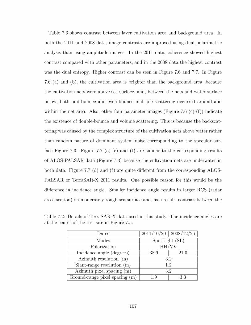
Table 7.3 shows contrast between laver cultivation area and background area. In

both the 2011 and 2008 data, image contrasts are improved using dual polarimetric

analysis than using amplitude images. In the 2011 data, coherence showed highest

contrast compared with other parameters, and in the 2008 data the highest contrast

was the dual entropy. Higher contrast can be seen in Figure 7.6 and 7.7. In Figure

7.6 (a) and (b), the cultivation area is brighter than the background area, because

the cultivation nets were above sea surface, and, between the nets and water surface

below, both odd-bounce and even-bounce multiple scattering occurred around and

within the net area. Also, other four parameter images (Figure 7.6 (c)-(f)) indicate

the existence of double-bounce and volume scattering. This is because the backscat-

tering was caused by the complex structure of the cultivation nets above water rather

than random nature of dominant system noise corresponding to the specular sur-

face Figure 7.3. Figure 7.7 (a)-(c) and (f) are similar to the corresponding results

of ALOS-PALSAR data (Figure 7.3) because the cultivation nets are underwater in

both data. Figure 7.7 (d) and (f) are quite different from the corresponding ALOS-

PALSAR or TerraSAR-X 2011 results. One possible reason for this would be the

difference in incidence angle. Smaller incidence angle results in larger RCS (radar

cross section) on moderately rough sea surface and, as a result, contrast between the

Table 7.2: Details of TerraSAR-X data used in this study. The incidence angles areat the center of the test site in Figure 7.5.

Dates 2011/10/20 2008/12/26

Modes SpotLight (SL)Polarization HH/VV

Incidence angle (degrees) 38.9 21.0Azimuth resolution (m) 3.2

Slant-range resolution (m) 1.2Azimuth pixel spacing (m) 3.2

Ground-range pixel spacing (m) 1.9 3.3

107

Figure 7.6: Comparison of image contrast between laver cultivation area and back-ground using TerraSAR-X HH/VV dual-polarization data in 2011. The values nextto each caption are mean contrasts. (a) HH+VV image: 0.001. (b) HH-VV image:0.327. (c) Entropy image: 0.253. (d) Scattering angle image: 0.348. (e) HH/VVcoherence image: 0.674. (f) Phase difference image: 0.226.

laver cultivation area and the background area could increase. Direct comparison

cannot be made between the PALSAR and TerraSAR-X results because of different

system parameters such as wavelengths and resolution. However, on a whole, these

results are comparably effective to the previous entropy based approaches which re-

quire full polarization data [66, 67] since we demonstrated that similar results can

be obtained using only HH and VV dual-polarization data. The dual entropy was

effective for both ALOS-PALSAR and TerraSAR-X data. Further, when full polar-

ization data are available, even better result can be attained by focusing on surface

scattering component.

108

Figure 7.7: Comparison of image contrast between laver cultivation area and back-ground using TerraSAR-X HH/VV dual-polarization data in 2008. The values nextto each caption are mean contrasts. (a) HH+VV image: 0.254. (b) HH-VV image:0.244. (c) Entropy image: 0.465. (d) Scattering angle image: 0.008. (e) HH/VVcoherence image: 0.031. (f) Phase difference image: 0.008.

Table 7.3: Image contrast between laver cultivation area and background area usingTerraSAR-X HH/VV dual-polarization data (Figure 7.5, 7.6 and 7.7).

Mean contrastParameter 2011/10/20 2008/12/26

HH 0.141 0.259VV 0.053 0.241

HH+VV 0.001 0.254HH-VV 0.327 0.244Entropy 0.253 0.465

Scattaring angle 0.348 0.008Coherence 0.674 0.031

Phase Difference 0.226 0.008

109

Chapter 8

Conclusions

In Chapter 1, SAR history and recent trends are introduced and the purpose of this

study is stated.

In Chapter 2, SAR image forming processes are summarised. The pulse compression

technique using a matched filtering for frequency modulated pulses is used to achieve

fine resolution in range direction. In azimuth direction, the technique of aperture

synthesis is used to construct an imaginary long aperture to produce fine resolution

in the azimuth direction. The SAR fundamentals given in this chapter serve as a

foundation for understanding and analysing SAR images.

In Chapter 3, the basic theory of SAR polarimetry, followed by the two major ana-

lytical methods of PolSAR data, the model-based decomposition and the eigenvalue

decomposition analyses, are described. SAR polarimetry has become increasingly

popular in recent years because the fully polarimetric SAR data contain much de-

tailed information than the single polarization SAR data.

In Chapter 4, the four-component scattering power decomposition (4-CSPD) algo-

110

rithm with rotation of covariance matrix is introduced. We demonstrated that the

algorithm is correct by showing that the result of covariance matrix rotation is iden-

tical to that of coherency matrix rotation utilizing ALOS-PALSAR quad-polarization

data. Although it is well known that the both matrices should produce the same re-

sult based on the theory of unitary transformation, experimental proof with rotation

of the matrices has not been done before. We also gave a warning against extreme

value ambiguity in determining rotation angle to minimize cross polarized component,

and showed how it can be avoided. We clarified that different types of areas react to

the rotation algorithm differently. Urban or industrial areas showing strong double-

bounce scattering with the original 4-CSPD (without rotation) are little affected by

rotation. Forested areas show random distribution in rotation angles because of their

randomness in polarization. Sea or smooth ground surface areas are moderately af-

fected by rotation. Urban or industrial areas which have oblique structures to radar

illumination show peaks of rotation angle distribution away from zero degree (center)

unlike the other areas, and the degree seems to correspond to the angle between the

radar illumination and the structures. We also showed that the rotation can improve

the classification of man-made objects such as ships and bridges on the sea.

In Chapter 5, In this study, we made clear the difference in eigenvalue analysis

between quad-, HH/VV dual-, and HH/HV dual polarization SAR data. The two-

dimensional correlation coefficients between the parameters derived from the quad

entropy/alpha decomposition and from the HH/VV dual entropy/alpha decomposi-

tion were sufficiently close, suggesting that the HH/VV dual entropy/alpha decom-

position can be used as an approximation for HH/VV dual-polarization data with

faster computational time suited for real-time application. Although HH/HV alpha

angle seems not very useful, HH/HV entropy can also be used as approximation for

quad entropy.

111

In Chapter 6, we suggested that the model-based decomposition analyses can be

effectively used to detect objects on the sea surface. We proposed two approaches

utilising the decomposed result. One approach is to subtract a specific scattering

component from the total power (i.e. to use the decomposed result as a band-stop

filter) to reveal intended targets by removing the effect of dominant scattering com-

ponent in the area. Although the main scattering component from the sea is surface

scattering, volume scattering can be a dominant scattering component when the sea

is very calm. This filtering method is shown to be more effective when the scattering

from the sea surface is strong. Also, this approach can be used to extract targets in

an area where there is a dominant scattering component. For example, man-made

objects in the forest can be extracted by filtering out volume scattering. The other

approach is to enhance double-bounce scattering, which is often inherent in scattering

from man-made objects. This approach was found to be more robust when the sea is

calm. We also confirmed that the detection capability of fully polarimetric SAR data

is not really limited by their spatial resolution. Our approach showed that objects

that are smaller than the spatial resolution can be detected utilizing polarimetric

information.

In Chapter 7, the image contrasts between laver cultivation area and background

area were evaluated using various parameters derived from multi-polarization data.

Unlike previous studies, this study clarified the relative performance between different

polarimetric analyses. As a result, it has been found that when the cultivation nets are

underwater, entropy performs better among dual-polarization methods, and surface

scattering calculated from 4-CSPD shows higher contrast than any other parameters

from fully polarimetric data. TerraSAR-X HH/VV dual-polarization data were also

analyzed, and the use of dual-polarization analysis turned out to be also effective on

TerraSAR-X data. This study could also be applied to detect polluted area caused by

tanker accident or offshore-oil disaster since spilled oil on the sea has similar physical

112

characteristics to laver cultivation area.

113

Bibliography

[1] K. Ouchi, Principles of Synthetic Aperture Radar for Remote Sensing (in

Japanese). Tokyo Denki University Press: Tokyo, second ed., 2009.

[2] J. C. Curlander and R. N. McDonough, Synthetic Aperture Radar: Systems and

Signal Processing. Wiley: New York, 1991.

[3] K. Ouchi, “Recent trend and advance of synthetic aperture radar with selected

topics,” Remote Sensing, vol. 5, no. 2, pp. 716–807, 2013.

[4] D. L. Evans, W. Alpers, A. Cazenave, C. Elachi, T. Farr, D. Glackin, B. Holt,

L. Jones, W. T. Liu, W. McCandless, Y. Menard, R. Moore, and E. Njoku,

“Seasat- 25-year legacy of success,” Remote Sensing of Environment, vol. 94,

no. 3, pp. 384–404, 2005.

[5] E. Rodriguez and J. Martin, “Theory and design of interferometric synthetic

aperture radars,” Radar and Signal Processing, IEE Proceedings F, vol. 139,

no. 2, pp. 147–159, 1992.

[6] D. Massonnet and K. L. Feigl, “Radar interferometry and its application to

changes in the Earth’s surface,” Review of Geophysics, vol. 36, no. 4, pp. 441–

500, 1998.

[7] A. Ferretti, C. Prati, and F. Rocca, “Permanent scatterers in SAR interferom-

114

etry,” IEEE Transactions on Geoscience and Remote Sensing, vol. 39, no. 1,

pp. 8–20, 2001.

[8] G. E. Hilley, R. Burgmann, A. Ferretti, F. Novali, and F. Rocca, “Dynamics

of slow-moving landslides from permanent scatterer analysis,” Science, vol. 304,

no. 5679, pp. 1952–1955, 2004.

[9] R. M. Goldstein and H. A. Zebker, “Interferometric radar measurement of ocean

surface currents,” Nature, vol. 328, pp. 707–709, 1987.

[10] J. Toporkov, D. Perkovic, G. Farquharson, M. Sletten, and S. Frasier, “Sea sur-

face velocity vector retrieval using dual-beam interferometry: first demonstra-

tion,” IEEE Transactions on Geoscience and Remote Sensing, vol. 43, no. 11,

pp. 2494–2502, 2005.

[11] J. S. Lee and E. Pottier, Polarimetric Radar Imaging From Basics to Applica-

tions. Boca Raton, FL: CRC Press, 2009.

[12] Y. Yamaguchi, Radar Polarimetry From Basics to Applications: Radar Remote

Sensing using Polarimetric Information (in Japanese). The Institute of Elec-

tronics, Information and Communication Engineers: Tokyo, 2007.

[13] S. R. Cloude and E. Pottier, “A review of target decomposition theorems in radar

polarimetry,” IEEE Transactions on Geoscience and Remote Sensing, vol. 34,

no. 2, pp. 498–518, 1996.

[14] A. Freeman and S. Durden, “A three-component scattering model for polarimet-

ric SAR data,” IEEE Transactions on Geoscience and Remote Sensing, vol. 36,

no. 3, pp. 963–973, 1998.

[15] P. Wright, S. Quegan, N. Wheadon, and C. Hall, “Faraday rotation effects on

115

L-band spaceborne SAR data,” IEEE Transactions on Geoscience and Remote

Sensing, vol. 41, no. 12, pp. 2735–2744, 2003.

[16] A. Freeman and S. Saatchi, “On the detection of Faraday rotation in linearly po-

larized L-band SAR backscatter signatures,” IEEE Transactions on Geoscience

and Remote Sensing, vol. 42, no. 8, pp. 1607–1616, 2004.

[17] A. Freeman, “Calibration of linearly polarized polarimetric SAR data subject

to Faraday rotation,” IEEE Transactions on Geoscience and Remote Sensing,

vol. 42, no. 8, pp. 1617–1624, 2004.

[18] S. Cloude and K. Papathanassiou, “Polarimetric SAR interferometry,” IEEE

Transactions on Geoscience and Remote Sensing, vol. 36, no. 5, pp. 1551–1565,

1998.

[19] M. Shimada and Y. Osawa, “ALOS-2 science program and high resolution SAR

applications,” in Proceedings of SPIE 8528, Earth Observing Missions and Sen-

sors: Development, Implementation, and Characterization II, (Kyoto, Japan),

2012.

[20] Y. Okada, T. Hamasaki, M. Tsuji, M. Iwamoto, K. Hariu, Y. Kankaku, S. Suzuki,

and Y. Osawa, “Hardware performance of L-band SAR system onboard ALOS-

2,” in Proceedings of 2011 IEEE International Geoscience and Remote Sensing

Symposium (IGARSS), pp. 894–897, 2011.

[21] G. Margarit, X. Fabregas, J. Mallorqui, L. Pipia, and T. Borquetas, “Polari-

metric SAR interferometry simulator of complex targets,” Proceedings of IEEE

International Geoscience and Remote Sensing Symposium (IGARSS), pp. 2015–

2018, 2005.

[22] D. Turner and I. Woodhouse, “An icon-based synoptic visualization of fully po-

larimetric radar data,” Remote Sensing, vol. 4, pp. 648–660, 2012.

116

[23] M. Migliaccio, A. Gambardella, F. Nunziata, M. Shimada, and O. Isoguchi, “The

PALSAR polarimetric mode for sea oil slick observation,” IEEE Transactions on

Geoscience and Remote Sensing, vol. 47, no. 12, pp. 4032–4041, 2009.

[24] I. Ramsey, E., A. Rangoonwala, Y. Suzuoki, and C. Jones, “Oil detection in a

coastal marsh with polarimetric synthetic aperture radar (SAR),” Remote Sens-

ing, vol. 3, pp. 2630–2662, 2012.

[25] G. Margarit, J. Barba Milanes, and A. Tabasco, “Operational ship monitoring

system based on synthetic aperture radar processing.,” Remote Sensing, vol. 1,

pp. 375–392, 2009.

[26] G. Margarit, J. Mallorqui, J. Fortuny-Guasch, and C. Lopez-Martinez, “Ex-

ploitation of ship scattering in polarimetric SAR for an improved classification

under high clutter conditions,” IEEE Transactions on Geoscience and Remote

Sensing, vol. 47, no. 4, pp. 1224–1235, 2009.

[27] A. Marino, I. Hajnsek, and N. Walker, “Validating a ship detector based on the

notch filter with RADARSAT-2 fine quad-pol data,” in Proceedings of SEASAR,

(Tromsø, Norway), 2012.

[28] S. R. Cloude and E. Pottier, “An entropy based classification scheme for land ap-

plications of polarimetric SAR,” IEEE Transactions on Geoscience and Remote

Sensing, vol. 35, no. 1, pp. 68–78, 1997.

[29] M. I. Skolnik, Radar Handbook. McGraw-Hill: Boston, second ed., 1990.

[30] C. Oliver and S. Quegan, Understanding Synthetic Aperture Radar Images.

Artech House: London, 1998.

[31] M. Soumekh, Synthetic Aperture Radar Signal Processing with MATLAB Algo-

rithms. Wiley: New York, 1999.

117

[32] H. Skriver, M. Svendsen, and A. Thomsen, “Multitemporal C- and L-band po-

larimetric signatures of crops,” IEEE Transactions on Geoscience and Remote

Sensing, vol. 37, no. 5, pp. 2413–2429, 1999.

[33] M. Arii, J. J. van Zyl, and Y. Kim, “Measuring orientation and randomness of

vegetation using polarimetric SAR data,” in Proceedings of IEEE International

Geoscience and Remote Sensing Symposium (IGARSS), pp. 1195–1198, 2011.

[34] F. Meyer and J. Nicoll, “Prediction, detection, and correction of Faraday rotation

in full-polarimetric L-band SAR data,” IEEE Transactions on Geoscience and

Remote Sensing, vol. 46, no. 10, pp. 3076–3086, 2008.

[35] S. R. Cloude, Polarisation: Applications in Remote Sensing. Oxford University

Press, 2009.

[36] Y. Yamaguchi, T. Moriyama, M. Ishido, and H. Yamada, “Four-component scat-

tering model for polarimetric SAR image decomposition,” IEEE Transactions on

Geoscience and Remote Sensing, vol. 43, no. 8, pp. 1699–1706, 2005.

[37] E. Pottier and J.-S. Lee, “Application of the ⟨⟨H/A/α⟩⟩ polarimetric decom-

position theorem for unsupervised classification of fully polarimetric SAR data

based on the Wishart distribution,” in Proceedings of SAR Workshop: CEOS

Committee on Earth Observation Satellites; Working Group on Calibration and

Validation, (Toulouse, France), pp. 335–340, 1999.

[38] S.-E. Park and W. Moon, “Unsupervised classification of scattering mechanisms

in polarimetric SAR data using fuzzy logic in entropy and alpha plane,” IEEE

Transactions on Geoscience and Remote Sensing, vol. 45, no. 8, pp. 2652–2664,

2007.

[39] J.-S. Lee, M. Grunes, T. Ainsworth, L. jen Du, D. Schuler, and S. Cloude,

“Unsupervised classification using polarimetric decomposition and the complex

118

Wishart classifier,” IEEE Transactions on Geoscience and Remote Sensing,

vol. 37, no. 5, pp. 2249–2258, 1999.

[40] L. Ferro-Famil, E. Pottier, and J.-S. Lee, “Unsupervised classification of multi-

frequency and fully polarimetric SAR images based on the H/A/Alpha-Wishart

classifier,” IEEE Transactions on Geoscience and Remote Sensing, vol. 39,

no. 11, pp. 2332–2342, 2001.

[41] Y. Yajima, Y. Yamaguchi, R. Sato, H. Yamada, and W. M. Boerner, “POLSAR

image analysis of wetlands using a modified four-component scattering power

decomposition,” IEEE Transactions on Geoscience and Remote Sensing, vol. 46,

no. 6, pp. 1667–1673, 2008.

[42] L. Zhang, B. Zou, H. Cai, and Y. Zhang, “Multiple-component scattering model

for polarimetric SAR image decomposition,” IEEE Geoscience and Remote Sens-

ing Letters, vol. 5, no. 4, pp. 603–607, 2008.

[43] M. Arii, J. J. Van Zyl, and Y. Kim, “Adaptive model-based decomposition of

polarimetric SAR covariance matrices,” IEEE Transactions on Geoscience and

Remote Sensing, vol. 49, no. 3, pp. 1104–1113, 2011.

[44] J. J. Van Zyl, M. Arii, and Y. Kim, “Model-based decomposition of polarimetric

SAR covariance matrices constrained for nonnegative eigenvalues,” IEEE Trans-

actions on Geoscience and Remote Sensing, vol. 49, no. 9, pp. 3452–3459, 2011.

[45] O. Antropov, Y. Rauste, and T. Hame, “Volume scattering modeling in Pol-

SAR decompositions: Study of ALOS PALSAR data over boreal forest,” IEEE

Transactions on Geoscience and Remote Sensing, vol. 49, no. 10, pp. 3838–3848,

2011.

[46] Y. Yamaguchi, A. Sato, W. M. Boerner, R. Sato, and H. Yamada, “Four-

component scattering power decomposition with rotation of coherency matrix,”

119

IEEE Transactions on Geoscience and Remote Sensing, vol. 49, no. 6, pp. 2251–

2258, 2011.

[47] Y. Yamaguchi, Y. Yajima, and H. Yamada, “A four-component decomposition of

POLSAR images based on the coherency matrix,” IEEE Geoscience and Remote

Sensing Letters, vol. 3, no. 3, pp. 292–296, 2006.

[48] J. Lee, E. Krogager, T. Ainsworth, and W. Boerner, “Polarimetric analysis of

radar signature of a manmade structure,” IEEE Geoscience and Remote Sensing

Letters, vol. 3, no. 4, pp. 555–559, 2006.

[49] C. Lardeux, P.-L. Frison, C. Tison, J.-C. Souyris, B. Stoll, B. Fruneau, and

J.-P. Rudant, “Classification of tropical vegetation using multifrequency partial

SAR polarimetry,” IEEE Geoscience and Remote Sensing Letters, vol. 8, no. 1,

pp. 133–137, 2011.

[50] D. J. Crisp, The State-of-the-Art in Ship Detection in Synthetic Aperture Radar

Imagery. Edinburgh, Australia: Defence Science and Technology Organization

(DSTO) Information Science Laboratory, 2004.

[51] J.-S. Lee, M. R. Grunes, and E. Pottier, “Quantitative comparison of classifi-

cation capability: fully polarimetric versus dual and single-polarization SAR,”

IEEE Transactions on Geoscience and Remote Sensing, vol. 39, no. 11, pp. 2343–

2351, 2001.

[52] T. L. Ainsworth, J. P. Kelly, and J.-S. Lee, “Classification comparisons between

dual-pol, compact polarimetric and quad-pol SAR imagery,” ISPRS Journal of

Photogrammetry and Remote Sensing, vol. 64, no. 5, pp. 464–471, 2009.

[53] V. Turkar, R. Deo, S. Hariharan, and Y. S. Rao, “Comparison of classifica-

tion accuracy between fully polarimetric and dual-polarization SAR images,” in

120

Proceedings of IEEE International Geoscience and Remote Sensing Symposium

(IGARSS), (Vancouver, Canada), pp. 440–443, 2011.

[54] X. Li and J. Chong, “Processing of Envisat alternating polarization data for

vessel detection,” IEEE Geoscience and Remote Sensing Letters, vol. 5, no. 2,

pp. 271–275, 2008.

[55] F. J. Charbonneau, B. Brisco, R. K. Raney, H. McNairn, C. Liu, P. W. Vachon,

J. Shang, R. DeAbreu, C. Champagne, A. Merzouki, and T. Geldsetzer, “Com-

pact polarimetry overview and applications assessment,” Canadian Journal of

Remote Sensing, vol. 36, pp. S298–S315, 2010.

[56] S. R. Cloude, D. Goodenough, and H. Chen, “Compact decomposition theory,”

IEEE Geoscience and Remote Sensing Letters, vol. 9, no. 1, pp. 28 –32, 2012.

[57] R. K. Panigrahi and A. K. Mishra, “Comparison of hybrid-Pol with quad-Pol

scheme based on polarimetric information content,” International Journal of

Remote Sensing, vol. 33, no. 11, pp. 3531–3541, 2012.

[58] R. Guo, Y.-B. Liu, Y.-H. Wu, S.-X. Zhang, M.-D. Xing, and W. He, “Applying

H/α decomposition to compact polarimetric SAR,” IET Radar, Sonar Naviga-

tion, vol. 6, no. 2, pp. 61 –70, 2012.

[59] S. Cloude, “The dual polarization entropy/alpha decomposition: a PALSAR case

study,” in Proceedings of POLinSAR, (Frascati, Italy), 2007.

[60] Z. Shan, C. Wang, H. Zhang, and J. Chen, “H-α decomposition and alternative

parameters for dual polarization SAR data,” in PIERS Proceedings, (Suzhou,

China), pp. 1386–1390, 2011.

[61] A. Dhar, B. Gray, and C. Menges, “Comparison of dual and full polarimetric

entropy/alpha decompositions with TerraSAR-X, suitability for use in classifi-

121

cation,” in Proceedings of IEEE International Geoscience and Remote Sensing

Symposium (IGARSS), (Vancouver, Canada), pp. 456–458, 2011.

[62] T. Ainsworth, J.-S. Lee, and L. Chang, “Classification comparisons between dual-

pol and quad-pol sar imagery,” in Proceedings of IEEE International Geoscience

and Remote Sensing Symposium (IGARSS), pp. 164 –167, 2007.

[63] M. Migliaccio, F. Nunziata, A. Montuori, and R. Paes, “Single-look complex

COSMO-SkyMed SAR data to observe metallic targets at sea,” IEEE Journal

of Selected Topics in Applied Earth Observations and Remote Sensing, vol. 5,

no. 3, pp. 893–901, 2012.

[64] F. Nunziata, M. Migliaccio, and C. Brown, “Reflection symmetry for polarimetric

observation of man-made metallic targets at sea,” IEEE Journal of Oceanic

Engineering, vol. 37, no. 3, pp. 384–394, 2012.

[65] M. Sugimoto, K. Ouchi, and Y. Nakamura, “Four-component scattering power

decomposition algorithm with rotation of covariance matrix,” Remote Sensing,

vol. 4, no. 8, pp. 2199–2209, 2012.

[66] E. S. Won, K. Ouchi, and C.-S. Yang, “Extraction of underwater laver cultiva-

tion nets by SAR polarimetric entropy,” IEEE Geoscience and Remote Sensing

Letters, vol. 10, no. 2, pp. 231–235, 2013.

[67] C.-S. Yang, S. K. Chaturvedi, J.-H. Song, and K. Ouchi, “Monitoring of ma-

rine laver cultivation using two ALOS-PALSAR PLR acquisition mode data,” in

Proceedings of APSAR, (Seoul, South Korea), 2011.

[68] M. Sugimoto and K. Ouchi, “Extraction of lavar cultivation area using SAR dual

polarization data,” in PIERS Proceedings, (Moscow, Russia), pp. 952–956, 2011.

122

[69] D. Velotto, M. Migliaccio, F. Nunziata, and S. Lehner, “Dual-polarized

TerraSAR-X data for oil-spill observation,” IEEE Transactions on Geoscience

and Remote Sensing, vol. 49, no. 12, pp. 4751–4762, 2011.

123

Academic Achievements

Journal Publications

(1) M. Sugimoto, K. Ouchi, and Y. Nakamura, “Four-component scattering power

decomposition algorithm with rotation of covariance matrix,” Remote Sensing,

vol. 4, no. 8, pp. 2199-2209, 2012.

(2) 杉本光伸, 大内和夫, 中村康弘, “ポラリメトリック SARにおけるCoherency行列

と共分散行列の回転４成分分解アルゴリズムの等価性評価と回転角の曖昧さにつ

いて,” 日本リモートセンシング学会誌, vol. 33, no. 2, pp. 117-125, 2013.

(3) M. Sugimoto, K. Ouchi, and Y. Nakamura, “Comprehensive contrast comparison

of laver cultivation area extraction using parameters derived from polarimetric

SAR data,”’ Journal of Applied Remote Sensing, vol. 7, no. 1, 073566, 2013.

(4) M. Sugimoto, K. Ouchi, and Y. Nakamura, “On the novel use of model-based de-

composition in SAR polarimetry for target detection on the sea,” Remote Sensing

Letters. (accepted for publication)

(5) M. Sugimoto, K. Ouchi, and Y. Nakamura, “On the similarity between dual- and

quad-eigenvalue analysis in SAR polarimetry,” Remote Sensing Letters. (under

rewiew)

(6) A. Marino, M. Sugimoto, K. Ouchi and I. Hajnsek, “A Notch Filter for ship

detection with polarimetric ALOS-PALSAR data: Tokyo Bay,” IEEE Journal

of Selected Topics in Applied Earth Observations and Remote Sensing. (under

review)

124

Conference Publications (international)

(1) M. Sugimoto, N. Shiroto, and K. Ouchi, “Estimation of ocean waveheight using

polarization ratio of synthetic aperture radar data,” Proceedings of IEEE In-

ternational Geoscience and Remote Sensing Symposium (IGARSS), (Vancouver,

Canada), pp. 2821-2824, 2011.

(2) M. Sugimoto, N. Shiroto, and K. Ouchi, “Ocean waveheight estimation using

polarization ratio of synthetic aperture radar data,” PIERS Proceedings, (Suzhou,

China), 2011.

(3) M. Sugimoto and K. Ouchi, “On the SAR image classification by rotation of

the covariance matrix in the four-component scattering power decomposition,”

PIERS Online, (Suzhou, China), vol. 7 no. 8, pp.756-760, 2011.

(4) M. Sugimoto and K. Ouchi, “Rotation of polarimetric matrices and its effects on

classification accuracy of man-made structures by synthetic aperture radar,” 2011

3rd International Asia-Pacific Conference on Synthetic Aperture Radar (AP-

SAR), (Seoul, Korea), pp. 598-601, 2011.　

(5) M. Sugimoto and K. Ouchi,“Extraction of lavar cultivation area using SAR dual

polarization data,” PIERS Proceedings, (Moscow, Russia), pp. 952-956, 2012.

(6) M. Sugimoto and K. Ouchi, “Comparison of alternative parameters to dual po-

larization SAR data,” SPIE Proceedings, (Edinburgh, UK), vol. 8536, 2012.

(7) M. Sugimoto, K. Ouchi, and Y. Nakamura, “On the coastal target detection

using dual and quad polarization SAR data,” Electronic Proceedings of ISRS

2012 ICSANE, (Incheon, Korea), 2012.

(8) M. Sugimoto, K. Ouchi, and Y. Nakamura, “Comparison of parameters derived

125

from dual-polarzation SAR data and their application,” 2012 International Sym-

posium on Antennas and Propagation (ISAP), (Nagoya, Japan), 2012.　

(9) M. Sugimoto, K. Ouchi, and Y. Nakamura, “Comparison of contrast improvement

of extracted laver cultivation area using parameters derived from polarimetric

SAR data,” SPIE Proceedings, (Kyoto, Japan), vol. 8525, 2012.

(10) M. Sugimoto, A. Marino, K. Ouchi, and Y. Nakamura, “A novel ship detection

method using model-based decomposition as a polarimetric band-stop filter,”

Proceedings of POLinSAR, (Frascati, Italy), 2013.

(11) M. Sugimoto, K. Ouchi, and C.-S. Yang,“On the eigenvalue analysis using HH-

VV dual-polarization SAR data and its applications to monitoring of coastal

oceans,” Electronic Proc. SPIE Defense, Security, and Sensing, (Baltimore,

USA), 2013.

126

Conference Publications (domestic)

(1) 杉本光伸, 大内和夫, “SARデータにおける共分散行列の回転を用いた４成分散

乱分解アルゴリズム,” 日本リモートセンシング学会第 50回学術講演会論文集,

pp.137-140, 2011.

(2) 杉本光伸, 大内和夫, “On the ambiguity and comparison of four-component scat-

tering power decomposition with rotation of coherency and covariance matrices

in SAR polarimetry”, 日本リモートセンシング学会第 51回学術講演会論文集,

pp.21-22, 2011.

(3) 杉本光伸, 大内和夫, “全偏波データに対する２偏波データにおける代用パラメー

タの検討,” 計測自動制御学会 第 19回リモートセンシングフォーラム, pp.31-32,

2012.

(4) M. Sugimoto and K. Ouchi, “合成開口レーダデータにおけるHH-VVコヒーレン

スを用いた２偏波分解,” 2012年電子情報通信学会総合大会講演論文集, B-2-34,

2012

(5) M. Sugimoto, K. Ouchi, and Y. Nakamura, “Comparison of alternative parame-

ters for dual polarization SAR data,” 日本リモートセンシング学会第 52回学術

講演会論文集, pp.259-260, 2012

(6) M. Sugimoto, K. Ouchi, and Y. Nakamura, “On the coastal information extrac-

tion using dual and quad polarization SAR data,” The 34th RESES Symposium,

2012.

(7) M. Sugimoto, K. Ouchi, and Y. Nakamura, “Extraction of laver cultivation area

using parameters derived from dual polarization SAR Data,” 日本リモートセン

シング学会第 53回学術講演会論文集, pp.115-116, 2012.

127

(8) 杉本光伸, 大内和夫, 中村康弘, “ALOS-PALSAR FBD 2偏波データによる 2008

年岩手・宮城内陸地震被害地域の抽出,” 日本リモートセンシング学会第 53回学

術講演会論文集, pp.45-46, 2012.

(9) 杉本光伸, 大内和夫, 中村康弘, “ポラリメトリック SARデータにおける船舶検出

のための新しい 4-COMP-Sフィルタの提案,”電子情報通信学会技術研究報告, vol.

112, no. 330, pp.37-40, 2012.

128

Awards

(1) 優秀論文発表賞, “On the ambiguity and comparison of four-component scattering

power decomposition with rotation of coherency and covariance matrices in SAR

polarimetry,” 日本リモートセンシング学会第 51回学術講演会, 2011.

(2) 財団法人　電気通信普及財団　海外渡航旅費援助

国際学会 SPIE Remote Sensing 2012 での口頭発表（題目：Comparison of alter-

native parameters to dual polarization SAR data）の際の渡航旅費援助

129