Seismic interferometry, intrinsic losses and Q-estimation *

Geophysical Prospecting, 2010, 58, 361–373 doi: 10.1111/j.1365-2478.2009.00828.x

Seismic interferometry, intrinsic losses and Q-estimation∗

Deyan Draganov†, Ranajit Ghose, Elmer Ruigrok, Jan Thorbeckeand Kees WapenaarDepartment of Geotechnology, Delft University of Technology, PO Box 5048, 2600 GA Delft, the Netherlands

Received December 2008, revision accepted July 2009

ABSTRACTSeismic interferometry is the process of generating new seismic traces from the cross-correlation, convolution or deconvolution of existing traces. One of the startingassumptions for deriving the representations for seismic interferometry by cross-correlation is that there is no intrinsic loss in the medium where the recordings areperformed. In practice, this condition is not always met. Here, we investigate theeffect of intrinsic losses in the medium on the results retrieved from seismic inter-ferometry by cross-correlation. First, we show results from a laboratory experimentin a homogeneous sand chamber with strong losses. Then, using numerical mod-elling results, we show that in the case of a lossy medium ghost reflections willappear in the cross-correlation result when internal multiple scattering occurs. Wealso show that if a loss compensation is applied to the traces to be correlated, theseghosts in the retrieved result can be weakened, can disappear, or can reverse theirpolarity. This compensation process can be used to estimate the quality factor in themedium.

INTRODUCTION

In its most general definition, seismic interferometry is theprocess of generating new seismic responses from the cross-correlation, convolution, or deconvolution of existing traces.Claerbout (1968) proposed to retrieve the reflection responseof a 1D medium from the autocorrelation of the transmissionresponse. Later, he conjectured that for a 3D medium, thereflection response could be retrieved from cross-correlationof observed seismic noise (Rickett and Claerbout 1996). Sincethe beginning of this century, different researchers have shownhow one can extract the seismic impulse response (the Green’sfunction) from the cross-correlation of observations fromtransient or noise sources (e.g., see Schuster 2001; Campilloand Paul 2003; Shapiro and Campillo 2004). For an exten-sive overview, the reader is referred to Schuster (2009) andWapenaar, Draganov and Robertsson (2008a). Lately, the

∗This paper is based on the extended abstract G024 presented at the70th EAGE Conference & Exhibition Incorporating SPE EUROPEC2008, 9–12 June 2008 in Rome, Italy.†E-mail: [email protected]

theory has been extended to electromagnetic and electro-seismic observations (Wapenaar, Slob and Snieder 2006;Slob, Draganov and Wapenaar 2007; Wapenaar et al.2006).

One of the main assumptions in seismic interferometry bycross-correlation is that there are no intrinsic losses in themedium where the recordings are made. Starting with thisassumption and consequently making use of the principle oftime-reversal invariance of the wave equation, it is shown that,taking the acoustic case as an example, the Green’s functionG(xA, xB, t) and its time-reversed version, that would be mea-sured at a receiver at point xA due to an impulsive source at xB,can be obtained from the relation (Wapenaar and Fokkema2006):

G (xA, xB, t) + G (xA, xB,−t)

≈ 2ρc

∮∂D

G (xB, x, t) ∗ G (xA, x, −t) d2x. (1)

In the above relation, c and ρ are the constant propagationvelocity and mass density, respectively, at and outside sur-face ∂D that effectively surrounds xA and xB and ∗ denotes

C© 2009 European Association of Geoscientists & Engineers 361

362 D. Draganov et al.

convolution. In the right-hand side of the above equationone cross-correlates recordings at the points xA and xB, whenthese recordings result from sources at positions x on the sur-face ∂D. Relation (1) is obtained from an exact equation asthe latter is not very useful for practical applications. Theexact equation contains in its right-hand side two integralsof cross-correlations of responses from monopole and dipolesources. To transform it to the more practical relation (1) withone integral of cross-correlations of responses from monopolesources only, it has been assumed that the dominant wave-lengths of the fields are small compared to the size of theinhomogeneities (high-frequency approximation) and that ∂D

is a sphere with a very large radius (far-field approximation).These approximations result in mainly amplitude errors.

When there are intrinsic losses in the medium of inter-est, Snieder (2006, 2007) showed that equation (1) shouldbe extended to include at the two observation points cross-correlations from sources inside the complete volume D en-closed by the boundary ∂D:

G (xA, xB, t) + G (xA, xB, −t)

≈ 2ρc

∮∂D

G (xB, x, t) ∗ G (xA, x, −t) d2x

+∫

D

(bp (x, t) + bp (x, −t)) ∗ G (xB, x, t) ∗ G (xA, x, −t) d3x,

(2)

where, following the notation of Wapenaar et al. (2006), bp(x)is the medium’s loss factor related to the compressibility. Theloss factor related to the mass density has been assumed tobe zero. In practical applications for laboratory or field ex-periments, the condition of a lossless medium will not alwaysbe met. This means that to apply seismic interferometry, onewould need to resort to equation (2). However, in general itwill be very difficult to find a situation where there would be adistribution of sources inside the complete volume of interest.The situation would become even more complicated, if theloss factor related to the mass density is not zero. In this case,a second volume integral would appear on the right-hand sideof equation (2) with cross-correlation at the two observationpoints of recordings from dipole sources in D, whereas inequation (2) the volume integration is only over recordingsfrom monopole sources.

It is most likely that in real situations the sources in themedia will only be confined to some small part (or severalparts) of the volume, which means that one should look foralternatives to equation (2). One alternative, which accountsfor intrinsic losses, was introduced by Slob et al. (2007) (seealso Halliday and Curtis (2009) for an application to scat-

tered surface waves). They proposed to use seismic interfer-ometry by convolution, where one of the observation pointsshould be outside the boundary ∂D, while the other observa-tion point should still lie inside ∂D. Even though this methodneeds only a surface integral over the sources, it is not al-ways a practical solution as in most seismic applications bothreceivers will be inside ∂D. Recently, Wapenaar, Slob andSnieder (2008b) proposed an alternative that accounts forintrinsic losses – seismic interferometry by multidimensionaldeconvolution. One extra advantage of seismic interferometryby multidimensional deconvolution is that it can compensatefor irregular source distribution and different source strengths.An additional requirement of the deconvolution method isthat a matrix inversion is made of simultaneous recordingsat many receivers to obtain the Green’s function between thetwo points of interest. Contrary to this, seismic interferometryby cross-correlation can be performed with recordings only atthe two points of interest. Vasconcelos and Snieder (2008a,b)proposed to use trace deconvolution before summation overthe sources on ∂D. This method does not require matrix in-version of simultaneous recordings but intrinsically assumes a1D medium.

For the above reasons, it will still be desirable to make useof relation (1) in a lot of practical applications. In the follow-ing, we investigate what are the effects of intrinsic losses onthe results from seismic interferometry by cross-correlation.We start our investigation using the simplest case – a homo-geneous model, and slowly increase the degree of difficultyby using a layered model and finally a general inhomoge-neous model with internal scattering. Slob et al. (2007) usednumerical modelling results for electromagnetic waves in atwo-layer medium with intrinsic losses to test the electromag-netic variant of equation (1). They showed that the cross-correlation method would still retrieve the Green’s functionbut that later arrivals might not be retrieved. In section ‘Lab-oratory results for a homogeneous sand chamber’ we test thisfinding on a scalar-wavefield laboratory dataset for a homo-geneous medium. Tanter, Thomas and Fink (1998) showedthat to improve the result of the application of time-reversalacoustics (a method related to seismic interferometry by cross-correlation) for focusing in the brain through the scull, i.e, inthe presence of losses, a loss compensation should be appliedbefore time reversal. In section ‘Modelling results for inhomo-geneous media’, we will work out a similar approach for seis-mic interferometry and will further show how our approachcan be used to estimate the effective quality factor (Q) of theoverburden.

C© 2009 European Association of Geoscientists & Engineers, Geophysical Prospecting, 58, 361–373

Seismic interferometry, intrinsic losses and Q-estimation 363

LABORATORY R E SUL T S FOR AHOMOGENEOUS SAND CHAMBER

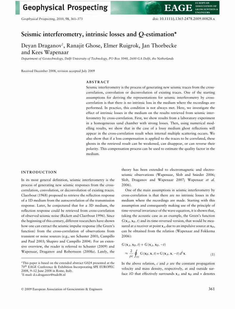
We start our investigation of the effect of intrinsic losses onthe results from SI by cross-correlation using a homogeneousphysical model. The goal was to directly check the effect of avarying damping, introduced by varying the source frequency,on the reflection response retrieved by cross-correlation. Thedata for this experiment were acquired in a water-tight cylin-drical chamber filled with unconsolidated sand, see Fig. 1.Special attention was paid to keep the sand in a loose, un-consolidated condition, because unconsolidated sand, withlow Q, causes strong attenuation of the propagating seismic-wave energy (e.g., see Musset and Khan 2000; Priest, Best andClayton 2005). The sand sample was prepared through pluvi-ation of sand in water making the sample quite homogeneous.

Figure 1 A homogeneous sand chamber for measuring transmission responses. S denotes a source of SH-waves and R denotes a receiver sensitivein the direction of the SH-wave motion. The red coordinate system indicates the orientation of the vertical axis z, the radius r and the azimuthφ. The sample consists of 34 plastic rings, each with a diameter of 225 mm and a height of 15 mm, except the lowest one, which was 6 mmhigh.

Figure 2 The measurements are performed using a ‘vanishing’ sample: after a measurement is finished, the top ring is sliced off and a newmeasurement is taken with the source placed at the new top.

The chamber consisted of 34 plastic (PVC) rings standing ona steel base. Piezoelectric bender elements served as sourceand receiver. The source and the receiver were positioned inthe middle points at the top and bottom of the sample, re-spectively. The measurements were performed following theidea of a ‘gradually vanishing sample’. The initial height of thesample was 501 mm. A source transducer acting as a sourcefor S-wave polarized in the horizontal direction (SH-wave)was placed on top of the sample at location S (see Fig. 1)and was set off. The resulting waves, transmitted through theunconsolidated sand, were recorded at the receiver locationR by a transducer sensitive in a direction parallel to the SH-wave polarization. After this, the top ring was carefully slicedoff, the source transducer was lowered to the new height ofthe sample, now 486 mm and a new transmission measure-ment was performed (Fig. 2). This procedure was repeated



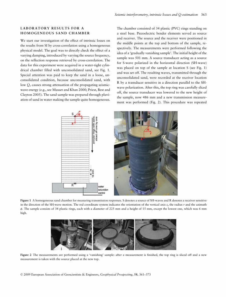
Figure 3 Observed transmission panels for the configuration in Fig. 1 for a source central frequency of a) 3 kHz, b) 6 kHz and c) 18 kHz. Thepanels are shown after application of automatic gain control to bring forward also the later arrivals. The yellow and green lines highlight thedirect transmission and its multiple, respectively.

until only the last ring was left. Note that this measurementscheme allowed us to measure the waves for different heightsof the sand sample and still keep the medium homogeneousfor each height level. The measurements resulted in 34 traces,combined in one panel (see Fig. 3).

Because we used both an SH-wave source and an SH-wavereceiver, the predominant energy in our recorded wavefieldwas SH and therefore, the wave propagation here was con-sidered to obey the scalar wave equation. However, due toimperfect coupling and finite dimensions of the transducerelements and due to the mode conversions at the chamberwall, some compressional (P) wave and vertically polarizedshear (SV) wave energy was also present in the data. Partic-ularly, P-wave arrivals were visible before the arrival of theearliest SH-waves. This energy was muted before further pro-cessing. Due to the cylindrical symmetry of the chamber, theexperiment could further be considered as independent of theazimuth.

For each source location three different measurements wereperformed by changing the central frequency of the source.The central frequencies were set to 3, 6 and 18 kHz, respec-tively. On the three resulting recorded panels shown in Fig. 3,we can observe the direct transmission arrival, highlighted bythe yellow lines and its multiple that had bounced between thebottom and the top of the sample, highlighted by the greenlines. We can also see reflections from the side walls of thechamber and their multiples. For our purposes, we concen-trated on the transmissions. From the transmission measure-ments we estimated the quality factor of the loose sand to be

around Q = 16. For this purpose, we used the band-limitedspectral ratio of the measurements (Tonn 1991). We did thisfor each source central frequency and then averaged the re-sults for the three frequency bands. Our estimated averagequality factor Q = 16 for shear waves in unconsolidated sandis realistic (e.g., Hu and Su 1999) have reported shear-waveQ < 10 for soft soil deposits and Q = 30 for weatheredbedrock at a shallow depth). In the following, we assumethat the estimated average Q is the same for all three datasets corresponding to the three different source frequencies.In reality, the effective damping for the three experiments isdifferent and increases with increasing frequency of the sourcewavelet. This can be seen in Fig. 3, where, due to strong atten-uation of the high frequencies, the frequency content of themiddle and right panels is not too much different from theone of the left panel.

We apply seismic interferometry to the observed transmis-sions with the aim to retrieve reflections between the top andthe bottom of the chamber. We use the modified form ofequation (1) for coinciding observation points, i.e.,

G (xR, xR, t) + G (xR, xR, −t)

≈ 2ρc

G (xR, xS, t) ∗ G (xR, xS, −t) . (3)

Because the source S and the receiver R lie on the cylinder’saxis and due to the cylindrical symmetry of the sand sample,for the retrieval of the reflection response we can suffice withonly one source at the top of the sample and thus the inte-gral over different source positions is omitted. The results of



Figure 4 Reflection response of the sand chamber for coincident source and receiver positions at the bottom of the sample at R. Retrievedreflection response was obtained from the autocorrelation of the observed transmission responses for source central frequencies of a) 3 kHz,b) 6 kHz and c) 18 kHz. For comparison purposes, (d) shows a finite-difference modelled reflection response. The event highlighted in redrepresents the reflection from the top of the cylindrical sample. The event highlighted in blue represents the multiple reflection that has bouncedtwice from the top of the chamber. The panels are shown after application of automatic gain control to bring forward also the later arrivals.

the application of equation (3) to the transmission measure-ments for the three different source frequencies are shown inFig. 4(a-c). Here the negative times were muted and automaticgain control was applied to bring forward the later arrivals.We refrained from filtering the noisy data sets of the labo-ratory experiments and highlighting the top and bottom re-flected events, because we wanted to examine whether seismicinterferometry works well even when the signal has sufferedfrom strong attenuation. Each of the three panels representsthe retrieved reflection response of the vanishing sample forcoincident source and receiver positions at the bottom of thechamber. As no reflection measurements were performed dur-ing the laboratory experiment, to be able to evaluate the qual-ity of the retrieved results, we compared the results with anumerically modelled reflection response. The modelling wasperformed using a scalar finite-difference scheme. The modelrepresented a homogeneous medium limited from all sidesby reflecting boundaries. The propagation velocity and qual-ity factor were taken to be 90 m/s and 16, respectively, asestimated from the transmission data. We used a source cen-tral frequency of 3 kHz. The modelled reflection response isshown in Fig. 4(d). Comparing kinematically the retrieved re-sults with the modelled data, we see that the reflection fromthe top of the sample (the event highlighted with red) is re-trieved but the quality of the retrieved result decreases withincreasing central frequency of the source wavelet. In pan-els (4b) and (4c), the higher frequency signals are strongly

damped when the height of the sample increases. This resultsin a low signal-to-noise ratio and, consequently, the reflec-tion from the top is less clear. This observation is even moreconspicuous for the multiple reflection highlighted with blue,which has bounced twice off the chamber’s top. In Fig. 4(a)the multiple is readily interpretable, in Fig. 4(b) it is harderto discern, while in Fig. 4(c) it is drowned in the backgroundnoise generated by the correlation process. This example con-firms the conclusion of Slob et al. (2007) that in a dissipativemedium SI by cross-correlation would retrieve the Green’sfunction but in case of strong losses the later arrivals mightnot be retrieved well.

MODELLING R ESULTS FORINHOMOGENEOUS MEDIA

We saw that in the simplest case of a homogeneous mediumor a medium consisting of two layers, seismic interferometryby cross-correlation relation, i.e., equation (1), can be used toretrieve the kinematics of the Green’s function. In this section,we investigate a more complex situation, where the mediumcauses internal scattering, for example when internal multiplesare generated.

Horizontally layered subsurface

It is instructive to investigate first the influence of intrinsiclosses on a subsurface model, as depicted in Fig. 5(a), which



0

100

200

300

400

500

600

700

800

900

1000

1100

1200

Depth

(m

)

2000 3000 4000 5000 6000Horizontal distance (m)

Cp=1500 m/sρ=1000 kg/m3Q=35

Cp=2000 m/sρ=1500 kg/m3Q=45

Cp=2500 m/s Q=50ρ=3000 kg/m3

Cp=2800 m/s Q=52ρ=3000 kg/m3

Cp=2950 m/s Q=54 ρ=4500 kg/m3

xB xA xB

4000

)b()a(

0

100

200

300

400

500

600

700

800

900

1000

1100

1200

Horizontal distance (m)

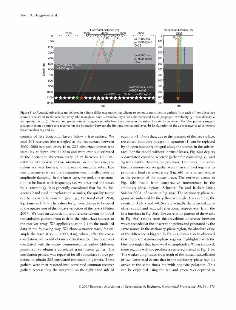
Figure 5 a) Acoustic subsurface model used in a finite-difference modelling scheme to generate transmission gathers from each of the subsurfacesources (the stars) to the receiver array (the triangles). Each subsurface layer was characterized by its propagation velocity cp, mass density ρ

and quality factor Q. The red and green pointers suggest raypaths from the sources in the subsurface to the receivers. The blue pointers suggesta raypath from a source to a receiver on the boundary between the first and the second layer. b) Explanation of the appearance of ghost eventsfor coinciding xA and xB .

consists of five horizontal layers below a free surface. Weused 201 receivers (the triangles) at the free surface between3000–5000 m placed every 10 m. 225 subsurface sources (thestars) lay at depth level 1100 m and were evenly distributedin the horizontal direction every 25 m between 1200 m–6800 m. We looked at two situations: in the first one, thesubsurface was lossless; in the second one, the subsurfacewas dissipative, where the dissipation was modelled only asamplitude damping. In the latter case, we took the attenua-tion to be linear with frequency, i.e, we described the lossesby a constant Q. It is generally considered that for the fre-quency band used in exploration seismics, the quality factorcan be taken to be constant (see, e.g., McDonal et al. 1958;Kjartansson 1979). The values for Q were chosen to be equalto the square root of the P-wave velocities of the layers (Mittet2007). We used an acoustic finite-difference scheme to modeltransmission gathers from each of the subsurface sources tothe receiver array. We applied equation (1) to the modelleddata in the following way. We chose a master trace, for ex-ample the trace at xB = (4000, 0 m), where, after the cross-correlation, we would obtain a virtual source. This trace wascorrelated with the entire common-source gather (differentpoints xA) to obtain a correlated transmission gather. Thecorrelation process was repeated for all subsurface source po-sitions to obtain 225 correlated transmission gathers. Thesegathers were then resorted into correlated common-receivergathers representing the integrand on the right-hand side of

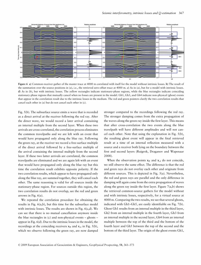
equation (1). Note that, due to the presence of the free surface,the closed boundary integral in equation (1) can be replacedby an open boundary integral along the sources in the subsur-face. For the model without intrinsic losses, Fig. 6(a) depictsa correlated common-receiver gather for coinciding xA andxB for all subsurface source positions. The traces in a corre-lated common-receiver gather were then summed together toproduce a final retrieved trace (Fig. 6b) for a virtual sourceat the position of the master trace. The retrieved events inFig. 6(b) result from constructive interference in thestationary-phase regions (Schuster, Yu and Rickett 2004;Snieder 2004) of events in Fig. 6(a). The stationary-phase re-gions are indicated by the yellow rectangle. For example, theevents at 0.26 s and −0.26 s are actually the retrieved zero-offset causal and acausal reflections, respectively, from thefirst interface in Fig. 5(a). The correlation pattern of the eventsin Fig. 6(a) results from the traveltime difference betweenwaves recorded at the observation points and generated by thesame source. In the stationary-phase region, the absolute valueof the difference is biggest. In Fig. 6(a) it can also be observedthat there are stationary-phase regions, highlighted with theblue rectangles that have weaker amplitudes. When summed,these regions will not produce a retrieved arrival in Fig. 6(b).The weaker amplitudes are a result of the mutual cancellationof two correlated events that in the stationary-phase regionsarrive at the same times but with opposite polarities. Thiscan be explained using the red and green rays depicted in



Figure 6 a) Common-receiver gather of the master trace at 4000 m correlated with itself for the model without intrinsic losses. b) The result ofthe summation over the source positions in (a), i.e., the retrieved zero-offset trace at 4000 m. c) As in (a), but for a model with intrinsic losses.d) As in (b), but with intrinsic losses. The yellow rectangles indicate stationary-phase regions, while the blue rectangles indicate coincidingstationary-phase regions that mutually cancel when no losses are present in the model. Gh1, Gh3, and Gh4 indicate non-physical (ghost) eventsthat appear in the correlation result due to the intrinsic losses in the medium. The red and green pointers clarify the two correlation results thatcancel each other in (a) but do not cancel each other in (c).

Fig. 5(b). The subsurface source emits a wave that is recordedas a direct arrival at the receiver following the red ray. Afterthe direct wave, we would record a later arrival containingan internal multiple from the second layer. When these twoarrivals are cross-correlated, the correlation process eliminatesthe common travelpaths and we are left with an event thatwould have propagated only along the blue ray. Followingthe green ray, at the receiver we record a free-surface multipleof the direct arrival followed by a free-surface multiple ofthe arrival containing the internal multiple from the secondlayer. If these two latter arrivals are correlated, the commontravelpaths are eliminated and we are again left with an eventthat would have propagated only along the blue ray but thistime the correlation result exhibits opposite polarity. If thetwo correlation results, which appear to have propagated onlyalong the blue ray, are summed together, they will cancel eachother. The same reasoning is valid for all sources inside thestationary-phase region. For sources outside this region, thetwo correlation results do not overlap, see the red and greenarrows in Fig. 6(a).

We repeated the correlation procedure for obtaining theresults in Fig. 6(a,b), but this time for the subsurface modelwith intrinsic losses. The results are shown in Fig. 6(c,d). Wecan see that there is no mutual cancellation anymore insidethe blue rectangles in (c) and non-physical events – ghosts –appear in Fig. 6(d). Due to the intrinsic losses in the model, therecordings at the coinciding receivers xB and xA in Fig. 5(b),which we observe following the green ray, are now damped

stronger compared to the recordings following the red ray.The stronger damping comes from the extra propagation ofthe waves along the green ray inside the first layer. This meansthat after cross-correlation the two events along the bluetravelpath will have different amplitudes and will not can-cel each other. Note that using the explanation in Fig. 5(b),the resulting ghost event will appear in the final retrievedresult at a time of an internal reflection measured with asource and a receiver both lying on the boundary between thefirst and second layers (Ruigrok, Draganov and Wapenaar2008).

When the observation points xB and xA do not coincide,we still observe the same effect. The difference is that the redand green rays do not overlay each other and originate fromdifferent sources. This is depicted in Fig. 5(a). Nevertheless,the red and green rays are parallel and the only difference indamping will again come from the extra propagation of wavesalong the green ray inside the first layer. Figure 7(a,b) showsthe retrieved common-source gathers for the model withoutand with intrinsic losses, respectively, for a virtual source at4000 m. Comparing the two results, we see that several ghosts,indicated with Gh1–Gh5, are easily identifiable on Fig. 7(b).Ghost Gh1 results from an internal multiple in the third layer,Gh2 from an internal multiple in the fourth layer, Gh3 froman internal multiple in the second layer, Gh4 from an internalmultiple between the top of the third and the bottom of thefourth layer and Gh5 between the top of the second and thebottom of the third layer. The origin of the ghost events Gh1,



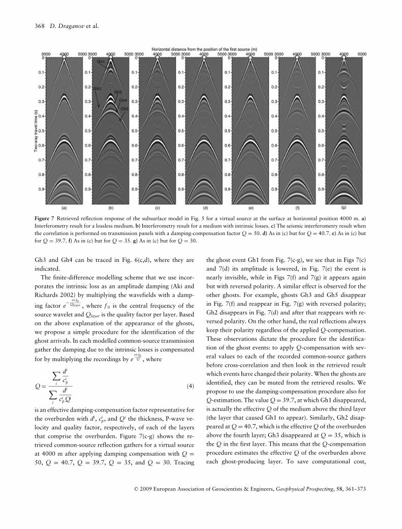
Figure 7 Retrieved reflection response of the subsurface model in Fig. 5 for a virtual source at the surface at horizontal position 4000 m. a)Interferometry result for a lossless medium. b) Interferometry result for a medium with intrinsic losses. c) The seismic interferometry result whenthe correlation is performed on transmission panels with a damping-compensation factor Q = 50. d) As in (c) but for Q = 40.7. e) As in (c) butfor Q = 39.7. f) As in (c) but for Q = 35. g) As in (c) but for Q = 30.

Gh3 and Gh4 can be traced in Fig. 6(c,d), where they areindicated.

The finite-difference modelling scheme that we use incor-porates the intrinsic loss as an amplitude damping (Aki andRichards 2002) by multiplying the wavefields with a damp-

ing factor e− tπ f0

Qlayer , where f 0 is the central frequency of thesource wavelet and Qlayer is the quality factor per layer. Basedon the above explanation of the appearance of the ghosts,we propose a simple procedure for the identification of theghost arrivals. In each modelled common-source transmissiongather the damping due to the intrinsic losses is compensated

for by multiplying the recordings by etπ f0

Q , where

Q =

∑i

di

cip

∑i

di

cipQi

(4)

is an effective damping-compensation factor representative forthe overburden with di, ci

p, and Qi the thickness, P-wave ve-locity and quality factor, respectively, of each of the layersthat comprise the overburden. Figure 7(c-g) shows the re-trieved common-source reflection gathers for a virtual sourceat 4000 m after applying damping compensation with Q =50, Q = 40.7, Q = 39.7, Q = 35, and Q = 30. Tracing

the ghost event Gh1 from Fig. 7(c-g), we see that in Figs 7(c)and 7(d) its amplitude is lowered, in Fig. 7(e) the event isnearly invisible, while in Figs 7(f) and 7(g) it appears againbut with reversed polarity. A similar effect is observed for theother ghosts. For example, ghosts Gh3 and Gh5 disappearin Fig. 7(f) and reappear in Fig. 7(g) with reversed polarity;Gh2 disappears in Fig. 7(d) and after that reappears with re-versed polarity. On the other hand, the real reflections alwayskeep their polarity regardless of the applied Q-compensation.These observations dictate the procedure for the identifica-tion of the ghost events: to apply Q-compensation with sev-eral values to each of the recorded common-source gathersbefore cross-correlation and then look in the retrieved resultwhich events have changed their polarity. When the ghosts areidentified, they can be muted from the retrieved results. Wepropose to use the damping-compensation procedure also forQ-estimation. The value Q = 39.7, at which Gh1 disappeared,is actually the effective Q of the medium above the third layer(the layer that caused Gh1 to appear). Similarly, Gh2 disap-peared at Q = 40.7, which is the effective Q of the overburdenabove the fourth layer; Gh3 disappeared at Q = 35, which isthe Q in the first layer. This means that the Q-compensationprocedure estimates the effective Q of the overburden aboveeach ghost-producing layer. To save computational cost,



Q might be estimated using only two receivers, instead ofapplying the procedure to the complete receiver array. Figure8(a-g) show the Q-estimation using the zero-offset traces fromFig. 7(a-g), respectively.

General inhomogeneous subsurface

In a more general inhomogeneous medium, the ghosts dueto the intrinsic losses can be identified by applying the Q-

0

0.1

0.2

0.3

0.4

Tw

o-w

ay tra

vel tim

e (

s)

Relative amplitude

Gh1

Gh3

Gh4

(a) (b) (c) (d) (e) (f) (g)

Figure 8 Retrieved zero-offset traces at horizontal position 4000 mfor the subsurface model from Fig. 5, a) without intrinsic losses, b)with intrinsic losses and when damping compensation is applied with(c) Q = 50, (d) Q = 40.7, (e) Q = 39.7, (f) Q = 35, and (g) Q = 30.All traces are scaled to the maximum amplitude in each trace.

0

100

200

300

400

500

600

700

800

900

1000

1100

1200

Depth

(m

)

2000 3000 4000 5000 6000Horizontal distance (m)

Cp=1500 m/sρ=1000 kg/m3Q=35

Cp=2000 m/sρ=1500 kg/m3Q=45

Cp=2500 m/s Q=50ρ=3000 kg/m3

Cp=2800 m/s Q=52ρ=3000 kg/m3

Cp=2950 m/s Q=54ρ=4500 kg/m3

xB xA

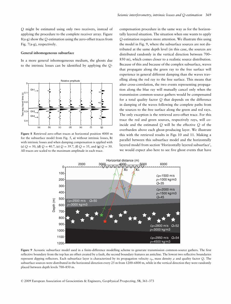
Figure 9 Acoustic subsurface model used in a finite-difference modelling scheme to generate transmission common-source gathers. The firstreflective boundary from the top has an offset created by a fault, the second boundary features an anticline. The lowest two reflective boundariesrepresent dipping reflectors. Each subsurface layer is characterized by its propagation velocity cp, mass density ρ and quality factor Q. Thesubsurface sources were distributed in the horizontal direction every 25 m from 1200–6800 m, while in the vertical direction they were randomlyplaced between depth levels 700–850 m.

compensation procedure in the same way as for the horizon-tally layered situation. The situation when one wants to applyQ-estimation requires more attention. We illustrate this usingthe model in Fig. 9, where the subsurface sources are not dis-tributed at the same depth level (in this case, the sources aredistributed randomly in the vertical direction between 700–850 m), which comes closer to a realistic source distribution.Because of this and because of the complex subsurface, wavesthat propagate along the green ray to the free surface willexperience in general different damping than the waves trav-elling along the red ray to the free surface. This means thatafter cross-correlation, the two events representing propaga-tion along the blue ray will mutually cancel only when thetransmission common-source gathers would be compensatedfor a total quality factor Q that depends on the differencein damping of the waves following the complete paths fromthe sources to the free surface along the green and red rays.The only exception is the retrieved zero-offset trace. For thistrace the red and green sources, respectively rays, will co-incide and the estimated Q will be the effective Q of theoverburden above each ghost-producing layer. We illustratethis with the retrieved results in Figs 10 and 11. Making aparallel between this subsurface model and the horizontallylayered model from section ‘Horizontally layered subsurface’,we would expect also here to see five ghost events that have



Figure 10 As in Fig. 7 but for the subsurface model from Fig. 9.

Gh

(a) (b) (c) (d) (e) (f) (g)

0

0.1

0.2

0.3

0.4

Tw

o-w

ay tra

vel tim

e (

s)

Relative amplitude

Figure 11 As in Fig. 8 but for the subsurface model from Fig. 9.

arisen due to the intrinsic losses. But due to the complexity ofthe subsurface model and source distribution, only one ghost,labelled Gh, is clearly visible in Fig. 10(b). This ghost wascaused by an internal multiple between the top of the secondlayer and the bottom of the third layer. Due to illuminationissues, the rest of the ghosts appear as correlation artefacts inboth the retrieved results without losses (Fig. 10a) and withlosses (Fig. 10b).

When we apply the Q-compensation procedure to thecommon-source transmission gathers and correlate them,looking at Fig. 10(c)-(g) we can easily identify the ghost. Onthe other hand, it is more difficult to conclude which Q causedthe ghost to disappear – panels Fig. 10(d,e) both appear toproduce the best results. Thus, we might conclude that the

effective Q of the overburden is around 40. When we look atthe zero-offset traces in Fig. 11 though and follow Gh fromFig. 11(c-g), we see that the best compensation is achievedwith Q = 35 (Fig. 11f), which is the actual effective Q of theoverburden, i.e., of the first layer.

D I S C U S S I O N

As shown above, application of seismic interferometry bycross-correlation to the response of a dissipative medium withinternal multiples will result in the appearance of ghost eventsin the retrieved result. These ghosts are comparable to the spu-rious multiples as described by Snieder, Wapenaar and Larner(2006) – both appear in the correlation results due to internalmultiple scattering. The difference is in the mechanisms thatlead to the appearance of the spurious multiples and the ghostevents. As Snieder et al. (2006) explained, spurious multipleswill appear in the case of one-sided illumination (for their ex-ample, when in an unbounded medium sources are availableonly above the receivers). The ghost events that we describewill appear in a dissipative medium even in the case of anisotropic illumination by the sources, which for the case ofFig. 9 means to have subsurface sources distributed alonga semicircle. For the unbounded-medium model in Sniederet al. (2006), we can link the two mechanisms if we imaginethe one-sided illumination as caused by a layer with extremely



low quality factor lying below the receivers and absorbing allthe energy from sources below it.

In section ‘General inhomogeneous subsurface’ we identi-fied only one ghost as caused by the losses. The other ghosts,which we expect to see due to internal multiples, are nowpresent also for the lossless situation in Fig. 10(a) becausethe subsurface source aperture is limited. Using the depictionwith the red and green sources in Fig. 9, this would mean,for example, that the red source is available, while the greenone is not. As a result, the event along the blue ray will notbe compensated. In the general case, it will not be possibleto recognize such illumination ghosts as non-physical arrivalsunless we know the subsurface velocity model and the sourcedistribution. In practice, though, parts of a non-physical ar-rival might appear as illumination ghosts and other parts asghosts due to losses. In this case, the Q-compensation proce-dure would help to identify the latter parts and consequentlythe complete non-physical arrival.

Ghosts related to intrinsic losses will appear not only dueto internal multiples but due to any scattering. Snieder et al.(2008) showed how spurious arrivals, caused by a scattererin an otherwise homogeneous lossless medium, cancel eachother when the illumination from the surrounding sources isisotropic. The cancelling terms are caused on the one handby cross-correlation of direct and scattered waves and on theother by cross-correlation of two scattered waves. In a lossymedium, these two terms will not cancel mutually as one ofthem will be weaker. Halliday and Curtis (2009) showed thisfor surface waves in scattering dissipative media.

In their time-reversal experiment in the presence of dissipa-tion, Tanter et al. (1998) assumed the absorbing object (theskull) to be a very thin layer and showed with experimentalresults that in practice this can be taken to be the case. Thatthe skull acts as a very thin layer means that no internal mul-tiples are generated by it. For this reason the authors havenot observed any ghosts after the application of time-reversedimaging. Their compensation factor simply counterbalancesthe direction-dependent intrinsic losses. The improvement oftheir result after loss compensation means that such a com-pensation should improve also our results in Fig. 4(a-c), i.e.,the retrieved reflections should become clearer. In our case,though, the Q-compensation resulted also in boosting of thecorrelation artefacts (resulting from correlation of terms otherthan only the transmissions, for example correlation of thetransmissions with the reflections from the sides of the cham-ber) and the overall picture did not improve.

We considered the case of a constant-Q intrinsic-loss mech-anism, which causes only amplitude changes in the modelled

transmission gathers. In practice, intrinsic losses might alsocause phase changes in the recorded signals. It needs to be in-vestigated whether the simple amplitude-compensation proce-dure we proposed would be sufficient to identify loss-relatedghosts in this case. If this appears to be insufficient, one shouldconsider a different intrinsic-loss mechanism during theQ-compensation procedure.

In section ‘General inhomogeneous subsurface’ we showedthat in realistic situations it will be difficult to use theQ-compensation procedure also for estimation of the effec-tive Q of the overburden. The best possibilities are providedby the zero-offset traces, assuming that subsurface sourcesare available in the stationary-phase region for the internalmultiples. If one is able to identify all ghosts caused by theinternal multiples until a certain depth level by applicationof the Q-compensation procedure, like in Fig. 7, one couldestimate the quality factor of each layer using equation (4) inan iterative scheme. This, of course, assumes that one has in-formation about the subsurface velocity structure. When onlya few ghosts can be identified, like in Fig. 10, one has a moredifficult task as one would not know unambiguously whichlayer caused a certain ghost to appear.

If one is only interested in the identification and removal ofghosts due to losses, Ruigrok et al. (2009) proposed to use asimpler procedure. A first retrieval result is produced when acorrelation is performed with a master trace that contains allarrivals. Then a second retrieval result is produced when thecorrelation is done with a master trace that contains only thedirect arrival. The amplitudes of ghost events in the secondresult should have increased compared to the amplitudes ofthe ghost events in the first result. This happens due to theremoval of the mutually canceling terms that should eliminatethe ghost events (Snieder et al. 2008; Vasconcelos and Snieder2009c). In practice, the difference in the amplitudes might bedifficult to see as it might be very small.

The Q-compensation procedure that we proposed for iden-tification of ghosts due to losses needs to be applied to trans-mission common-source gathers before cross-correlation. Thisprocedure will only work when separate recordings can bemade from each of the subsurface sources. In the case of seis-mic interferometry with white-noise sources in the subsurface,i.e., when the recordings are performed as if the subsurfacesources act simultaneously, the ghost events will not be iden-tifiable. In practical situations, though, the noise sources donot always act simultaneously. One can take advantage of thisand look at the noise records to identify arrivals from separatesubsurface sources. Then one can simulate records from sepa-rate subsurface sources, by extracting panels starting around



the first arrival and continuing for a few seconds. Draganov(2007) applied this technique to noise records from the MiddleEast and showed that the interferometry results improve whencompared to the interferometry results obtained using the to-tal noise records. When the panels are extracted, each of themshould be normalized with the amplitude of its first arrivalto compensate for possible unequal damping due to differentdepth and strength of the subsurface sources and unknownexact time of the first arrival. After that, the panels can beused in the Q-compensation procedure. The Q-compensationand estimation procedure can also be applied to surface wavesfollowing a similar preprocessing.

In elastodynamic dissipative media, one will encounter notonly loss-related ghosts arising due to P-waves but also ghostscaused by multiple scattering of S-waves and converted waves.Following equation (76) in Wapenaar and Fokkema (2006),one should apply the Q-compensation and estimation proce-dure to transmission gathers from separate P- and Sk-sources,where k = 1, 2, 3.

CONCLUSIONS

Seismic interferometry by cross-correlation assumes a losslessmedium. We showed that seismic interferometry by cross-correlation can be used also in a medium with intrinsiclosses. We showed with laboratory results from a homoge-neous medium that the kinematics of the Green’s functionare retrieved but that the later arrivals may not be retrieved.We showed that when multiple scattering occurs in the lossymedium, seismic interferometry by cross-correlation gives riseto non-physical events (ghosts) in the retrieved results. Theseghosts are a result of internal reflections inside layers lyingbetween the subsurface sources and the receivers. We showedthat by applying different Q-compensations to the recordedpanels before the cross-correlation, the ghost events can easilybe identified, because depending on the strength of the ap-plied compensation they are weakened, they disappear, or theychange their polarity. We also demonstrated that the ghostsdisappear when the applied Q-compensation corresponds tothe value of the effective Q of the overburden above eachof the ghost-producing layers. This can be used for effectiveQ-estimation.

ACKNOWLEDG ME N T S

We thank Karel Heller for his assistance in the lab experi-ments. The research of D.D., the research of R.G. and the labexperiments were financially supported by the Dutch Tech-

nology Foundation STW, applied science division of NWOand the technology programme of the Ministry of EconomicAffairs (grants VENI.08115 and DAR.5761). The research ofE.R. was financially supported by The Netherlands Organisa-tion for Scientific Research NWO (grant Toptalent 2006 AB).We thank the three anonymous reviewers for their very con-structive remarks, which helped to improve the manuscript.

REFERENCES

Aki K. and Richards P.G. 2002. Quantitative Seismology, 2nd edn.University Science Books.

Campillo M. and Paul A. 2003. Long-range correlations in the diffuseseismic coda. Science 299, 547–549.

Claerbout J.F. 1968. Synthesis of a layered medium from its acoustictransmission response. Geophysics 33, 264–269.

Draganov D. 2007. Seismic and electromagnetic interferometry: re-trieval of the Earth’s reflection response using crosscorrelation. PhDthesis, Delft University of Technology.

Halliday D. and Curtis A. 2009. Seismic interferometry of scatteredsurface waves in attenuative media. Geophysical Journal Interna-tional (in press).

Hu J.-F. and Su Y.-J. 1999. Estimation of the quality factor in theshallow soil using surface waves. Acta Seismologica Sinica 12, 81–487.

Kjartansson E. 1979. Constant Q-wave propagation and attenuation.Journal of Geophysical Research 84, 4737–4748.

McDonal J.F., Angona F.A., Mills R.L., Sengbush R.L., van NostrandR.G. and White J.E. 1958. Attenuation of shear and compressionalwaves in Pierre shale. Geophysics 23, 421–439.

Mittet R. 2007. A simple design procedure for depth extrapolation op-erators that compensate for absorption and dispersion. Geophysics72, S105–S112.

Musset A.E. and Khan M.A. 2000. Looking Into The Earth: An In-troduction to Geological Geophysics. Cambridge University Press.

Priest J.A., Best A.I. and Clayton C.R.I. 2005. Attenuation of seismicwaves in methane gas hydrate-bearing sand. Geophysical JournalInternational 164, 149–159.

Rickett J. and Claerbout J.F. 1996. Passive seismic imaging appliedto synthetic data. Stanford Exploration Project, pp. 87–94.

Ruigrok E., Draganov D. and Wapenaar K. 2008. Global-scale seis-mic interferometry: theory and numerical examples, GeophysicalProspecting 56, 395–417.

Ruigrok E., Wapenaar K., van der Neut J. and Draganov D. 2009.A review of crosscorrelation and multidimensional deconvolutionseismic interferometry for passive data. EAGE Workshop on Pas-sive Seismics, Limassol, Cyprus.

Schuster G.T. 2001. Theory of daylight/interferometric imaging: tuto-rial. 63rd EAGE meeting, Amsterdam, The Netherlands, ExtendedAbstracts, A–32.

Schuster G.T., Yu J. and Rickett J. 2004. Interferometric/daylightseismic imaging. Geophysical Journal International 157, 838–852.

Schuster G.T. 2009. Seismic Interferometry. Cambridge UniversityPress.



Shapiro N.M. and Campillo M. 2004. Emergence of broad-band Rayleigh waves from correlations of the ambientseismic noise. Geophysical Research Letters 31, L07614.doi:10.1029/2004GL019491.

Slob E., Draganov D. and Wapenaar K. 2007. Interferometric elec-tromagnetic Green’s functions representations using propagationinvariants. Geophysical Journal International 169, 60–80.

Snieder R. 2004. Extracting the Green’s function from the correlationof coda waves: a derivation based on stationary phase. PhysicalReview E 69, 046610-1–046610-8.

Snieder R. 2006. Retrieving the Green’s function of the diffusionequation from the response to a random forcing. Physical ReviewE 74, 046620.

Snieder R., Wapenaar K. and Larner K. 2006. Spurious multiples inseismic interferometry of primaries. Geophysics 71, SI111–SI124.

Snieder R. 2007. Extracting the Green’s function of attenuating het-erogeneous acoustic media from uncorrelated waves. Journal of theAcoustic Society of America 121, 2637–2643.

Snieder R., van Wijk K., Haney M. and Calvert R. 2008. Thecancellation of spurious arrivals in Green’s function extractionand the generalized optical theorem. Physical Review E 78,036606.

Tanter M., Thomas J.-L. and Fink M. 1998. Focusing and steeringthrough absorbing and aberrating layers: Application to ultrasonic

propagation through the skull. Journal of the Acoustic Society ofAmerica 103, 2403–2410.

Tonn R. 1991. The determination of the seismic quality factor Qfrom VSP data: a comparison of different computational methods.Geophysical Prospecting 39, 1–27.

Vasconcelos I. and Snieder R. 2008a. Interferometry by deconvolu-tion, Part 1 - Theory for acoustic waves and numerical examples.Geophysics 73(3), S115–S128.

Vasconcelos I. and Snieder R. 2008b. Interferometry by deconvolu-tion, Part 2 - Theory for elastic waves and application to drill-bitseismic imaging, Geophysics 73, S129–S141.

Vasconcelos I. and Snieder R. 2009c. Representation theorems andGreen’s function retrieval for scattering in acoustic media. PhysicalReview E (in press).

Wapenaar K. and Fokkema J. 2006. Green’s functions representationsfor seismic interferometry. Geophysics 71, SI33–SI46.

Wapenaar K., Slob E. and Snieder R. 2006. Unified Green’s functionretrieval by cross-correlation. Physical Review Letters 97, 234301-1–234301-4.

Wapenaar K., Draganov D. and Robertsson J.O.A. 2008a. SeismicInterferometry: History and Present Status. SEG.

Wapenaar K., Slob E. and Snieder R. 2008b. Seismic and electromag-netic controlled-source interferometry in dissipative media. Geo-physical Prospecting 56, 419–434.


Seismic interferometry, intrinsic losses and Q-estimation *

Documents

Transcript of Seismic interferometry, intrinsic losses and Q-estimation *