Intrinsic Thermoacoustic Instability of Premixed Flames

Thomas Emmert, Sebastian Bomberg, Wolfgang Polifke

Lehrstuhl fur ThermodynamikTechnische Universitat MunchenD-85747, Garching, Germany

Email: polifke@tum.de

Abstract

The thermoacoustic stability of velocity sensitive premix flames is investi-gated. A causal representation of the flow-flame-acoustic interactions revealsa flame-intrinsic feedback mechanism. The feedback loop may be describedas follows: An upstream velocity disturbance induces a modulation of theheat release rate, which in turn generates an acoustic wave traveling in theupstream direction, where it influences the acoustic velocity and thus closesthe feedback loop. The resonances of this feedback dynamics, which areidentified as intrinsic eigenmodes of the flame, have important consequencesfor the dynamics and stability of the combustion process in general and theflame in particular. It is found that the amplification of acoustic power byflame-acoustic interactions can reach very high levels at frequencies closeto the intrinsic eigenvalues due to the flame-internal feedback mechanism.This is shown rigorously by evaluating the “instability potentiality” from abalance of acoustic energy fluxes across the flame. One obtains factors ofmaximum (as well as minimum) power amplification. Based on the acous-tic energy amplification, the small gain theorem is introduced as a stabilitycriterion for the combustion system. It allows to formulate an optimizationcriterion for the acoustic characteristics of burners or flames without regardof the boundary conditions offered by combustor or plenum. The conceptsand methods are exemplified first with a simplistic n-τ model and then witha flame transfer function that is representative of turbulent swirl burners.

Keywords: intrinsic instability, premixed flame, acoustic energy,thermoacoustics, frequency response, open loop gain, combustion dynamics

Preprint submitted to Combustion and Flame July 1, 2014

Nomenclature

CWA Characteristic wave amplitudeF (s) Flame transfer function −f Downstream traveling CWA m s−1

g Upstream traveling CWA m s−1

H Energy amplification matrix −λmax Maximum sound power amplification −n Interaction index −ω Frequency rad s−1

Ω Closed loop denominator of flame feedback −OLTF Open loop transfer function of flame feedback −p′ Acoustic pressure fluctuation Pa~% Vector of emitted rescaled CWAs Ws Laplace variable (= jω + σ) rad s−1

σ Growth rate rad s−1

~ς Vector of incident rescaled CWAs WS Scattering matrix −Σ Energy scaled scattering matrix −τ Time delay sθ Relative temperature jump (= Td/Tu − 1) −u′ Acoustic velocity fluctuation m s−1

ξ Ratio of specific impedances (= ρu cu/ρd cd) −

Subscript indicesbf Burner and Flamef Flameu Upstreamd Downstream

1. Introduction

The dynamics and stability of flames are fascinating and multi-facetedphenomena, which have been important and popular topics in combustionresearch (Williams, 1985; Lewis and von Elbe, 1987). From a fundamentalpoint of view, thermo-diffusive or hydrodynamic flame instabilities mightbe most interesting (Clavin, 1985; Buckmaster, 1993; Matalon, 2007), whilephenomena such as blow off or flash back are very relevant for combustion

2

engineering, see e.g. Kroner et al. (2003); Aggarwal (2009); Cavaliere et al.(2013).

The present paper focuses on thermoacoustic instabilities, which resultfrom an interaction between fluctuations of heat release rate and acousticwaves (Rayleigh, 1878). Starting with the development of rocket engines inthe 1930’s, thermoacoustic instabilities have impeded severely the develop-ment of reliable combustion equipment. The development of lean-premixed,low-emission combustion technology for stationary gas turbines has increasedthe technological relevance of these instabilities, their prediction and controlremains a challenging task with great scientific appeal (Keller, 1995; Lieuwenand Yang, 2006).

Thermoacoustic instabilities are usually conceptualized as a coupled feed-back loop involving burner, flame, combustion chamber and plenum (possiblyalso fuel or air supply, etc): Fluctuations of heat release act as a monopolesource of sound (Strahle, 1971), the resulting acoustic waves are reflectedby the combustion chamber or the plenum and in turn modulate the flowconditions at the burner, which successively perturb the flame and thus closethe feedback loop (Keller, 1995; Dowling, 1995). If the resulting relativephase between fluctuations of heat release and pressure at the flame arefavourable, a self-excited instability may occur (Rayleigh, 1878). In thiswell-established framework, thermoacoustic instabilities are considered a re-sult of the combined dynamics of the flame and its acoustic environment, i.e.plenum, burner, combustor, supply lines, etc.; a flame placed in a anechoicenvironment should not be able to develop a thermoacoustic instability.

The present paper develops a different point of view: thermoacoustic in-teractions at the flame are analyzed in a framework that properly respectsthe causal relationships between “excitation” and “responses”, respectively.With this perspective, it becomes evident that flame-intrinsic feedback be-tween acoustics-flow-flame-acoustics may give rise to intrinsic flame instabil-ities, which are distinct from the resonating acoustic eigenmodes of the envi-ronment of the flame. Nevertheless, these instabilities are thermoacoustic innature, and thus differ essentially from other types of “intrinsic flame insta-bilities in premixed and non-premixed combustion”, as reviewed by Matalon(2007).

In an independent study, Hoeijmakers et al. (2014) explored strategiesfor preventing thermoacoustic instabilities by breaking the aforementionedfeedback loop and also observed that a flame can be intrinsically unstable.Experiments were carried out in a setup with significant acoustic losses, in-

3

duced by acoustic horns. The stability behaviour was investigated for threedifferent burners, and a range of operating conditions. It was observed thatdespite the significant acoustic losses present, thermoacoustic instabilitiesmay still occur (Hoeijmakers et al., 2013). Of course, these results are veryclosely related to the ideas developed in the present paper. Lending furthersupport to the argument, Bomberg et al. (2014) have identified intrinsic flameeigenmodes in experimental setups investigated previously by Noiray et al.(2007) and Komarek and Polifke (2010), respectively.

The paper is organized as follows: The next chapter introduces first thelow-order modelling concepts that are used to formulate ideas. Then the in-trinsic thermoacoustic feedback structure of a velocity-sensitive premix flameis identified. The corresponding spectrum of intrinsic eigenmodes is deter-mined for the simple example of an n-τ flame transfer function. In the sub-sequent section, a balance for the flow rates of acoustic energy at a premixflame is formulated, introducing the “instability potentiality” (Auregan andStarobinski, 1999; Polifke, 2011). It is found that frequencies where genera-tion of perturbation energy by fluctuating heat release is maximal correlatewith the intrinsic eigenfrequencies of the flame. Invoking the small gain the-orem originally deduced by Zames (1966), it is then shown how these resultsare related to a general stability criterion for network models. This leads toan optimization criterion for individual elements in acoustic networks, whichmight be used to optimize burner designs independently from up- or down-stream acoustic conditions at an early stage of combustor development. Thetools and concepts developed up to that point are then applied to a morerealistic flame transfer function, which is representative of turbulent premixswirl flames. The analysis in the present paper is formulated in terms of alow-order model for velocity sensitive premixed flames. Nevertheless, impli-cations should go beyond the limitations of the present study and indeed befairly general, as discussed in the conclusions.

2. Intrinsic Thermoacoustic Feedback in a Velocity-Sensitive Pre-mix Flame

Our investigation is focused on the dynamics of the coupling between theheat release of the flame and the acoustic waves incident to and emitted fromthe flame. There is a causal chain of events, consisting of the acoustic wavesaltering the flow field, which leads to a fluctuation in heat release, whichin turn generates acoustic waves. For premixed flames, the heat release

4

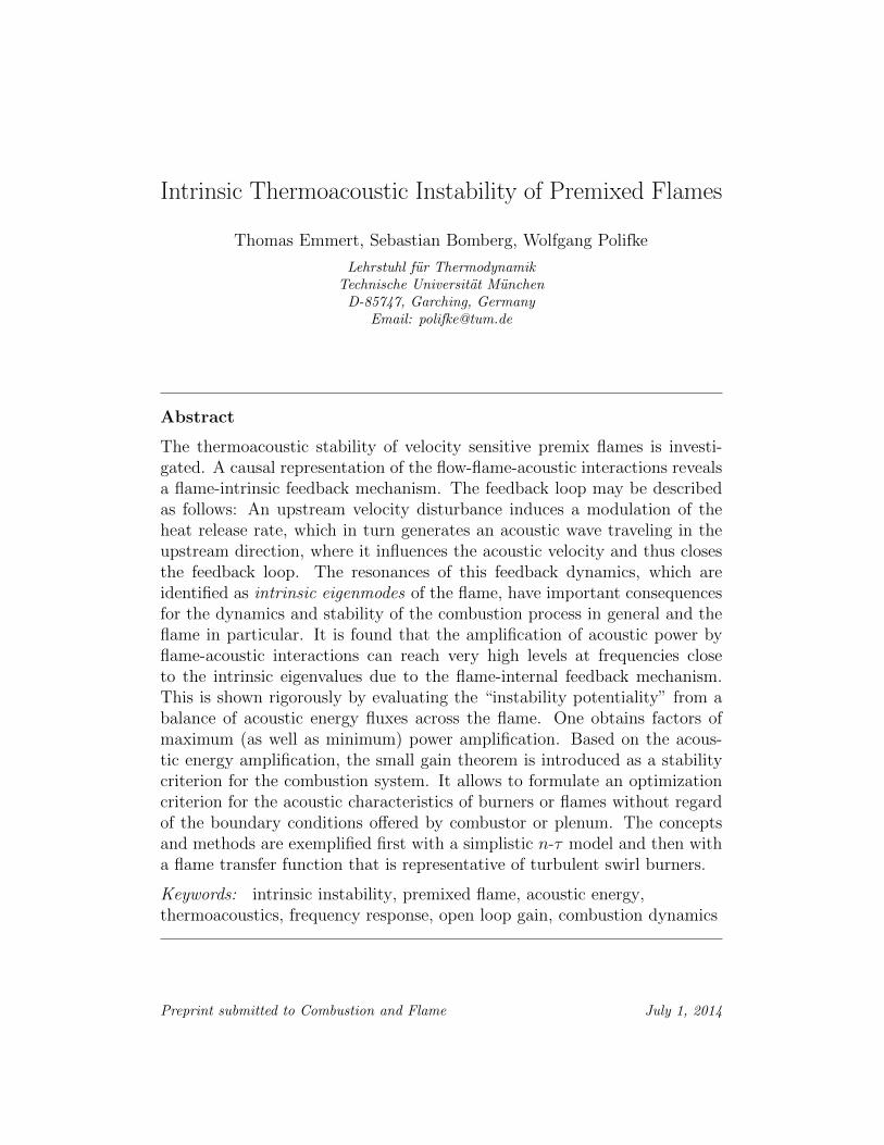
Figure 1: Velocity sensitive premixed flame anchored in a duct section.

fluctuation is typically caused by a velocity perturbation u′ upstream of theflame. Thus the flame does not respond directly to incident acoustic waves,but to an upstream flow perturbation. The physical mechanism involved maybe flame front kinematics, a convective transport of fuel inhomogeneities ora swirl modulation and possibly other effects.

For example in the case of premixed flames with technical fuel injection,a modulation of air velocity u′ at the location of fuel injection results in anequivalence ratio modulation φ′, which convects downstream. For an acous-tically ”stiff” injector, positive u′ gives a leaner mixture and negative u′ aricher mixture, whereas pressure p′ has no effect. Once the fuel inhomo-geneities arrive at the flame, they cause heat release rate fluctuations.

On the other hand, inside a swirler, in response to a perturbation ofvelocity, a wave in swirl number (or circulation) is set up, and the flameresponds later to the swirl modulation as shown by Straub and Richards(1999) as well as Komarek and Polifke (2010). Palies et al. (2011) have coinedthe term ”mode conversion” for this effect where an acoustic wave generatesa vortical wave. Again, the cause for this generation of swirl modulation isu′ at the swirler, p′ at the swirler is unimportant.

As a last example, according to the Unit Impulse Response model of theG-equation by Blumenthal et al. (2013), the ”restoration term” of the flamefront kinematics is triggered by movement of the flame at the anchoring point.The physical mechanism for this generic flame model may be vortex sheddingat a backward facing step. So again, u′ at the anchoring point is importantand the flame transfer functions respect this causality as they relate u′ to Q′.

Other than deducing causality from first principles, it is substantiallyharder to retrieve it from experiments. The reason is, that in frequencydomain, no discrimination between causes and consequences is possible andtherefore, no causality can be inferred from measured results of harmonic

5

solutions. But there is also numerical evidence for the causal relation betweena velocity perturbation and heat release fluctuations of laminar premixedflames. Jaensch et al. (2014) have identified and validated causal time domainmodels for the flame transfer function of such a flame from random time seriessimulation of a CFD model.

Low-order modeling concepts are used throughout this paper to formulateideas. The present chapter introduces very briefly pertinent nomenclatureand concepts, more details are found, e.g. in (Munjal, 1987; Dowling, 1995;Keller, 1995; Polifke, 2010; Tay-Wo-Chong et al., 2012). Then the intrin-sic thermoacoustic feedback structure of a ducted, velocity-sensitive premixflame as depicted in Fig. 1 is identified. The corresponding spectrum ofeigenmodes is determined for the simplistic example of an n-τ flame transferfunction. In Section 4 the method will be applied to a more complex modelof a turbulent premixed swirl burner.

2.1. Low-order thermoacoustic flame model

The diameter of the combustor configurations investigated is assumed tobe much smaller than relevant acoustic wave lengths. Therefore, acousticmodes are considered to consist of one dimensional plane waves. Underthe assumption of an acoustically compact flame with Helmholtz numberHe ≡ Lflame/λ 1, the conservation equations for mass, momentum andenergy may be linearized to relate fluctuations of heat release Q′ and acousticperturbations of velocity u′ and pressure p′ upstream (u) and downstream(d) of the flame to each other. To simplify the derivation, terms of orderO(2) in Mach number and higher are neglected and two non-dimensionalparameters are introduced: Ratio of specific impedances ξ ≡ ρucu

ρdcd, and the

relative temperature increase θ ≡ Td/Tu − 1. Fluctuating quantities aredenoted with a ’, mean flow quantities do not carry indices:(

p′

ρc

u′

)d

=

(ξ 00 1

)(p′

ρc

u′

)u

+

(0θuu

)Q′

Q. (1)

The first term on the r.h.s. describes the coupling of acoustic pressure p′

and velocity u′ across the discontinuity in specific impedances, the secondterm accounts for the effect of fluctuating heat release Q′. The originalderivation of these relations – known also as “acoustic Rankine-Hugoniotjump conditions” – was given by Chu (1953), a detailed derivation using thesame notation as this paper is found in (Kopitz and Polifke, 2008) or (Polifke,2010).

6

The system of Eqs. (1) has constant coefficients and is not closed as Q′

is unknown. Closure is achieved – and non-trivial dynamics are introduced– with a model for the heat release fluctuations of the flame: The flametransfer function F (s). As we are assuming a velocity sensitive flame, theheat release fluctuations Q′ are related to a velocity perturbation u′u upstreamof the flame:

Q′

Q= F (s)

u′uuu, (2)

where s = jω + σ is the Laplace variable. Various strategies to retrieve theflame transfer function F (s) are described in the literature. The most popularmethods are based on parametrized models such as the kinematic G-equation(Schuller et al. (2003), Lieuwen and Yang (2006)), and identification of non-parametric models from experiments (Paschereit et al., 2002) or reactive flowsimulations (Tay-Wo-Chong et al., 2012).

With the flame transfer function, closure of Eqns. (1) is achieved and onecan introduce a flame transfer matrix T(s):(

p′

ρc

u′

)d

=

(ξ 00 1 + θF (s)

)︸ ︷︷ ︸

T(s)

(p′

ρc

u′

)u

(3)

2.2. Causal representation of flame dynamcis and intrinsic feedback

The solution of the 1D wave equation can be represented as superpositionof characteristic waves traveling in opposite directions. On the perspectiveof the acoustic subsystem containing the flame, acoustic waves that are en-tering the domain are causal inputs “excitation”, while acoustic waves thatare leaving the domain are causal outputs ”responses”. The direction ofpropagation ensures causality in the sense that waves that are leaving thedomain are caused by waves that entered the domain at former times. Polifkeand Gentemann (2004) have shown, however, that the analysis of transmis-sion and reflection of acoustic waves by a multi-port is facilitated by usinga causal representation. The primitive acoustic variables p′ and u′ on theother hand are non-causal quantities in the sense that it is not possible toassociate unambiguously a direction of propagation with either of them.

The scattering matrix formulation provides a representation of acousticinteractions at an element. Characteristic acoustic wave amplitudes f, g are

7

introduced

f ≡ 1

2

(p′

ρc+ u′

); g ≡ 1

2

(p′

ρc− u′

)(4)

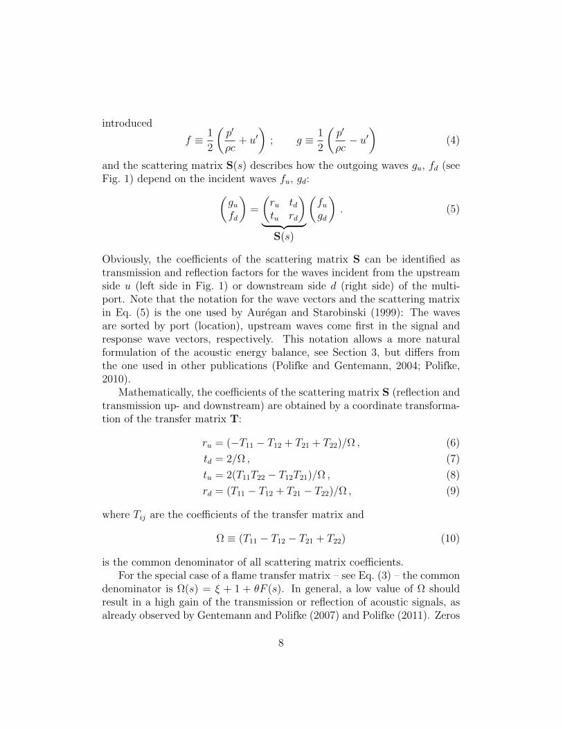
and the scattering matrix S(s) describes how the outgoing waves gu, fd (seeFig. 1) depend on the incident waves fu, gd:(

gufd

)=

(ru tdtu rd

)︸ ︷︷ ︸

S(s)

(fugd

). (5)

Obviously, the coefficients of the scattering matrix S can be identified astransmission and reflection factors for the waves incident from the upstreamside u (left side in Fig. 1) or downstream side d (right side) of the multi-port. Note that the notation for the wave vectors and the scattering matrixin Eq. (5) is the one used by Auregan and Starobinski (1999): The wavesare sorted by port (location), upstream waves come first in the signal andresponse wave vectors, respectively. This notation allows a more naturalformulation of the acoustic energy balance, see Section 3, but differs fromthe one used in other publications (Polifke and Gentemann, 2004; Polifke,2010).

Mathematically, the coefficients of the scattering matrix S (reflection andtransmission up- and downstream) are obtained by a coordinate transforma-tion of the transfer matrix T:

ru = (−T11 − T12 + T21 + T22)/Ω , (6)

td = 2/Ω , (7)

tu = 2(T11T22 − T12T21)/Ω , (8)

rd = (T11 − T12 + T21 − T22)/Ω , (9)

where Tij are the coefficients of the transfer matrix and

Ω ≡ (T11 − T12 − T21 + T22) (10)

is the common denominator of all scattering matrix coefficients.For the special case of a flame transfer matrix – see Eq. (3) – the common

denominator is Ω(s) = ξ + 1 + θF (s). In general, a low value of Ω shouldresult in a high gain of the transmission or reflection of acoustic signals, asalready observed by Gentemann and Polifke (2007) and Polifke (2011). Zeros

8

+

+ +

+

++

+_

Figure 2: Structure of the intrinsic feedback mechanism of a velocity sensitive premix flamewith the flame transfer function F (s) and the transmission and reflection coefficients ofthe scattering matrix Sξ.

of the denominator Ω(s) → 0 are poles of the flame scattering matrix. Itwill be shown in the following that the poles of the flame scattering matrixare not artifacts due to mathematical conversions from transfer to scatteringmatrix formulation, but indeed are due to intrinsic eigenmodes of the flameand associated resonances.

A re-formulation of the system of equations allows to develop a distinctphysical interpretation of the intrinsic modes: Instead of directly transform-ing the closed form flame transfer matrix Eq. (3) to scattering matrix for-mulation Eq. (5), the open form of the Rankine-Hugoniot jump conditionsEq. (1) is first rewritten in scattering matrix representation to obtain Sξ, i.e.the scattering matrix of the jump in specific impedances due to the steadyheat release. The thermoacoustic effect of the unsteady heat release is sub-sequently introduced, using again the flame transfer function Eq. (2). Thefollowing intermediate system of equations is obtained:(

gufd

)=

1

ξ + 1

(1− ξ 2

2ξ ξ − 1

)︸ ︷︷ ︸

Sξ

(fugd

)+

θ

ξ + 1

(1ξ

)F (s)(fu − gu) . (11)

The gu wave, which is propagating away from the flame in the upstreamdirection, is present on both sides of the equations. In the context of acausal representation of the system dynamics, with excitation on the r.h.s.and response on the l.h.s. (Polifke and Gentemann, 2004), this means thatthe wave amplitude gu appears as a cause as well as an effect and thus it

9

causes feed back within the flame model.The structure of this intrinsic feedback cycle is illustrated by the thick red

lines in the dynamic system sketch of the flame in Figure 2. The feedbackmechanism involves the upstream traveling wave gu, which contributes tothe velocity perturbation at the reference position “u” (see the lower leftcorner of the figure). The flame, which is velocity sensitive, responds witha fluctuation in heat release rate Q′, which in turn generates an upstreamtraveling wave gu.

It is important to notice that this intrinsic feedback is not visible intransfermatrix representation of the system in Eq. (3). The reason for thisdiscrepancy between scattering- and transfermatrix is that the transfermatrixis presuming gu = p′u

ρc−u′u as a input and therefore ignores the causal intrinsic

feedback mechanism.

2.3. Stability of intrinsic eigenmodes

The open loop dynamics of the feedback cycle introduced in the previoussubsection is described by the open loop transfer function (OLTF) and anegative feedback:

gu = − θ

ξ + 1F (s)︸ ︷︷ ︸

OLTF

gu . (12)

When solving for the closed loop transfer function dynamics of the scat-tering matrix of the flame, it is necessary to rewrite Eq. (11) such that guappears as output on the l.h.s.:(gufd

)=

1

ξ + 1 + θF (s)

(θF (s)− ξ + 1 22ξ(θF (s) + 1) ξ − 1− θF (s)

)︸ ︷︷ ︸

Sf

(fugd

)=

SfΩ

(fugd

).

(13)The matrix inversion involves a division of all coefficients of the scatteringmatrix with the factor Ω, which was introduced in Eq. (10). Now this factorcan be identified as the closed loop feedback dynamics corresponding to theopen loop feedback cycle of the flame (Eq. 12):

Ω = ξ + 1 + θF (s) = (ξ + 1) · (1 + OLTF(s)) . (14)

Thus, the roots s (zeros) of the closed loop denominator Ω(s) = 0 are theeigenvalues (poles) of the flame scattering matrix Sf (s). Roots of Ω corre-spond to OLTF = −1. The point Pcrit = −1 is called critical point. The

10

eigenmodes of the flame dynamics are stable if all eigenfrequencies corre-spond to negative growth rates and are unstable if they have positive growthrates.

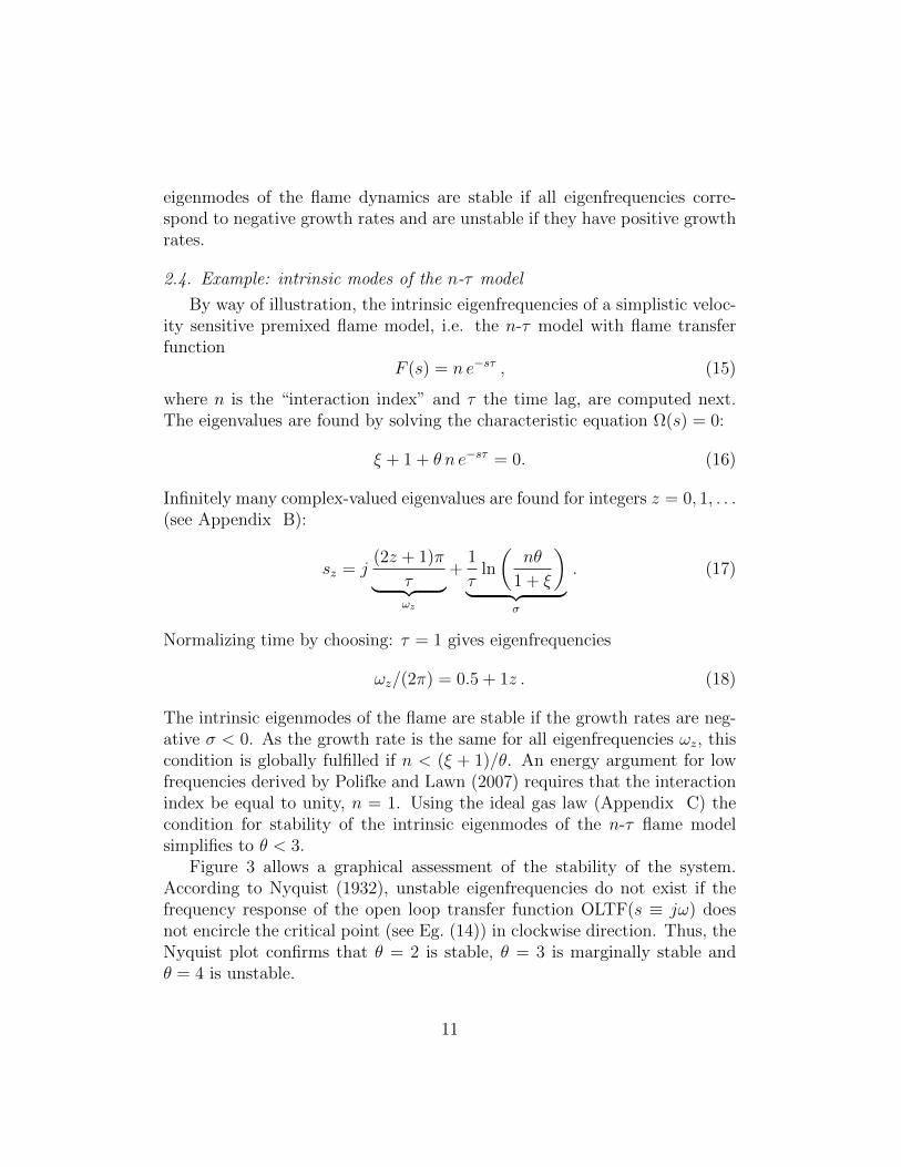
2.4. Example: intrinsic modes of the n-τ model

By way of illustration, the intrinsic eigenfrequencies of a simplistic veloc-ity sensitive premixed flame model, i.e. the n-τ model with flame transferfunction

F (s) = n e−sτ , (15)

where n is the “interaction index” and τ the time lag, are computed next.The eigenvalues are found by solving the characteristic equation Ω(s) = 0:

ξ + 1 + θ n e−sτ = 0. (16)

Infinitely many complex-valued eigenvalues are found for integers z = 0, 1, . . .(see Appendix B):

sz = j(2z + 1)π

τ︸ ︷︷ ︸ωz

+1

τln

(nθ

1 + ξ

)︸ ︷︷ ︸

σ

. (17)

Normalizing time by choosing: τ = 1 gives eigenfrequencies

ωz/(2π) = 0.5 + 1z . (18)

The intrinsic eigenmodes of the flame are stable if the growth rates are neg-ative σ < 0. As the growth rate is the same for all eigenfrequencies ωz, thiscondition is globally fulfilled if n < (ξ + 1)/θ. An energy argument for lowfrequencies derived by Polifke and Lawn (2007) requires that the interactionindex be equal to unity, n = 1. Using the ideal gas law (Appendix C) thecondition for stability of the intrinsic eigenmodes of the n-τ flame modelsimplifies to θ < 3.

Figure 3 allows a graphical assessment of the stability of the system.According to Nyquist (1932), unstable eigenfrequencies do not exist if thefrequency response of the open loop transfer function OLTF(s ≡ jω) doesnot encircle the critical point (see Eg. (14)) in clockwise direction. Thus, theNyquist plot confirms that θ = 2 is stable, θ = 3 is marginally stable andθ = 4 is unstable.

11

−1.5 −1 −0.5 0 0.5 1 1.5−1.5

−1

−0.5

0

0.5

1

1.5

θ=3

θ=2

Pcrit

Real Axis

Imag

inar

yA

xis

ω

θ=4

Figure 3: Nyquist plot with critical point of the open loop transfer function OLTF(s) ofthe n-τ flame model for various values of the relative temperature increment θ.

In an independent study, Hoeijmakers et al. (2014) computed eigenmodesof a simple thermoacoustic model system, with an n-τ heat source placedin a duct. Even in the limit of zero reflection coefficients, eigenmodes werefound. It is evident that these eigenmodes are associated with the instabilitiesresulting from flame-intrinsic feedback identified in the present study.

Given the stability of the flame alone, conclusions about the stability ofthe combustion system containing the flame cannot be drawn directly. It isa well known result from control theory that due to feedback, the stability ofa linear system is undetermined even if all parts of a system are individuallystable. In the present context, this means that even though a flame itselfmight be stable, given the right feedback of acoustic waves by the upstreaman downstream boundaries, the interconnected combustion system might beunstable. Thus there is the need for a weaker (more conservative) stabilitycriterion that allows to draw conclusions concerning thermoacoustic stabil-ity without regarding its boundaries. Such a criterion will be developed inSection 3.

3. Stability Criteria Based on a Balance of Acoustic Power

As stated in the previous section, the stability of a linear acoustic systemdepends on all constitutive elements, and can be determined only by theanalysis of the entire system. This approach can be tedious for large systems.

12

At an early stage of the design process, when the acoustic dynamics of allcomponents are not yet known, it may even be impossible. Thus it is ofinterest to develop a stability criterion based on perturbation energy or soundpower, which allows to optimize individual elements of the combustion systemindependently.

Derivations of perturbation energy in increasingly complex flows weredeveloped by Chu (1964), Cantrell et al. (1964), Morfey (1971), Myers (1991)and Giauque et al. (2006), Brear et al. (2012). A definition of perturbationenergy implies a decomposition of flow perturbations into acoustics, vorticesand entropy, but this decomposition is not unambiguously. More recentlyGeorge and Sujith (2012) have pointed out, that in fact, Myers decompositiondoes not fulfill certain properties one should expect from an energy norm,whereas Chu’s norm does, but it lacks the rigorous derivation.

The core issue is however that none of the norms leads to a conservativeenergy potential, which is needed for the construction of a rigorous stabil-ity criterion. Strictly speaking, energy provides a stability criterion onlyif it is monotonously decreasing for stable systems (Lyapunov and Fuller(1992), Rouche et al. (1977)). This does in general not apply to (acoustic)perturbation energy. Investigations by Subramanian and Sujith (2011), Blu-menthal et al. (2013), as well as Wieczorek et al. (2011) show that due to theacoustic-flow-flame-acoustic interaction even low order linear thermoacousticsystems are non-normal. As a consequence (acoustic) perturbation energymay rise even if the thermoacoustic system is asymptotically stable (“tran-sient growth”). The method we propose instead does not rely on the acousticenergy in the field and is therefore not affected by the issues mentioned above.

Based on a balance for sound power, Auregan and Starobinski (1999)introduced the whistling potentiality, which provides a necessary-but-not-sufficient criterion for instability in (aero-)acoustic multi-port systems. Po-lifke (2011) linked the argument of Auregan and Starobinski to commonlyused acoustic scattering matrices and applied the criterion under the nameinstability potentiality to a flame system. As instability potentiality is soundpower based, it is also linked to the Rayleigh criterion (see Brear et al.(2012)), though not limited by the strong assumptions of the latter. In thissection it will be shown that strong amplification ”gain” of sound power andthus strong potentiality of thermoacoustic instability occurs in the vicinityof the intrinsic eigenmodes of the flame.

Eventually, a rigorous theoretical science base is provided by linking theenergy or sound power based stability criterion to the small gain theorem,

13

which was originally developed by Zames (1966) in the domain of controlsystem theory.

process of a gas turbine combustion system.

3.1. Sound Power Balance

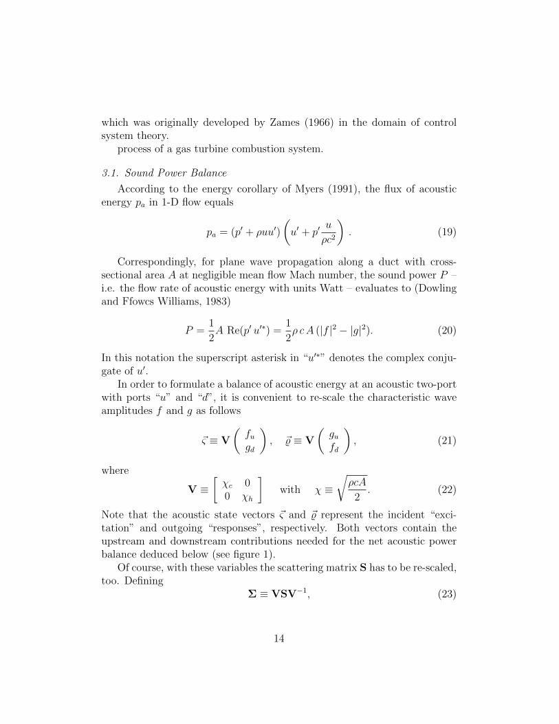
According to the energy corollary of Myers (1991), the flux of acousticenergy pa in 1-D flow equals

pa = (p′ + ρuu′)

(u′ + p′

u

ρc2

). (19)

Correspondingly, for plane wave propagation along a duct with cross-sectional area A at negligible mean flow Mach number, the sound power P –i.e. the flow rate of acoustic energy with units Watt – evaluates to (Dowlingand Ffowcs Williams, 1983)

P =1

2A Re(p′ u′∗) =

1

2ρ cA (|f |2 − |g|2). (20)

In this notation the superscript asterisk in “u′∗” denotes the complex conju-gate of u′.

In order to formulate a balance of acoustic energy at an acoustic two-portwith ports “u” and “d”, it is convenient to re-scale the characteristic waveamplitudes f and g as follows

~ς ≡ V

(fugd

), ~% ≡ V

(gufd

), (21)

where

V ≡[χc 00 χh

]with χ ≡

√ρcA

2. (22)

Note that the acoustic state vectors ~ς and ~% represent the incident “exci-tation” and outgoing “responses”, respectively. Both vectors contain theupstream and downstream contributions needed for the net acoustic powerbalance deduced below (see figure 1).

Of course, with these variables the scattering matrix S has to be re-scaled,too. Defining

Σ ≡ VSV−1, (23)

14

one formulates concisely for the scattering of acoustic waves by a two-port:

~% = Σ~ς. (24)

The re-scaled acoustic variables are energy-extensive, i.e. the 2-normof an acoustic state vector ~ς or ~% represents the corresponding flow rate ofacoustic energy P incident upon or emanating from a two-port, respectively:

Pin = ||~ς ||2 = ~ς †~ς, (25)

Pout = ||~% ||2 = ~% †~%. (26)

where (·)† denotes the complex conjugate transpose (the “adjoint”) of a vec-tor or matrix. The steady-state balance of acoustic power for a two-port nowreads as follows,

Pgen = Pout − Pin. (27)

The rate of generation of acoustic energy Pgen is the difference between inci-dent and outgoing acoustic flow rates. If Pgen > 0 incident acoustic power isamplified, i.e. there is overall generation of acoustic energy by the acoustictwo-port, if Pgen < 0 more power is dissipated than produced. CombiningEqns. (24) – (27), one finds that

Pgen = ~ς †(Σ†Σ︸︷︷︸H

)~ς − ~ς †~ς. (28)

This formulation makes explicit that the generation of acoustic energy by atwo-port is related to the non-unitary character of its scattering matrix Σ:Production Pgen = 0 if the scattering matrix is unitary, i.e. if its adjoint isequal to its inverse, Σ† = Σ−1.

Acoustic states that correspond to maximal (or minimal) generation ofacoustic energy can be identified by determining the eigenvectors ~εi andeigenvalues λi, i = 1, 2 of the energy amplification matrix H ≡ Σ†Σ. Follow-ing Auregan and Starobinski (1999), the sum of the energy of the incomingwaves is conveniently normalized to unity, ||~ς ||2 = 1. Then the energy of theoutgoing waves is equal to the value of the quadratic form ~ς †H~ς on the unitsphere, which can be reduced to a sum of squares:

~ς †H~ς =2∑i=1

λi|ηi|2. (29)

15

~"max

~"min

&u

&d

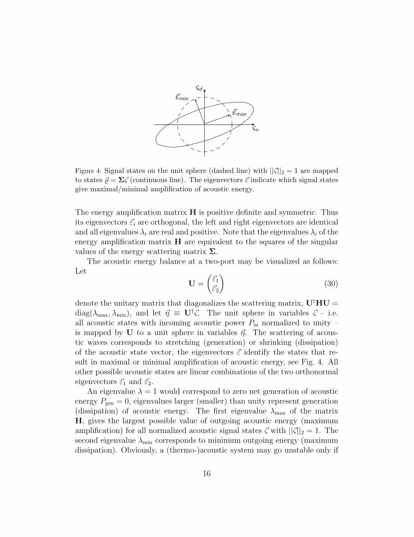
Figure 4: Signal states on the unit sphere (dashed line) with ||~ς||2 = 1 are mappedto states ~% = Σ~ς (continuous line). The eigenvectors ~ε indicate which signal statesgive maximal/minimal amplification of acoustic energy.

The energy amplification matrix H is positive definite and symmetric. Thusits eigenvectors ~εi are orthogonal, the left and right eigenvectors are identicaland all eigenvalues λi are real and positive. Note that the eigenvalues λi of theenergy amplification matrix H are equivalent to the squares of the singularvalues of the energy scattering matrix Σ.

The acoustic energy balance at a two-port may be visualized as follows:Let

U =

(~ε1~ε2

)(30)

denote the unitary matrix that diagonalizes the scattering matrix, U†HU =diag(λmax, λmin), and let ~η ≡ U†~ς. The unit sphere in variables ~ς – i.e.all acoustic states with incoming acoustic power Pin normalized to unity –is mapped by U to a unit sphere in variables ~η. The scattering of acous-tic waves corresponds to stretching (generation) or shrinking (dissipation)of the acoustic state vector, the eigenvectors ~ε identify the states that re-sult in maximal or minimal amplification of acoustic energy, see Fig. 4. Allother possible acoustic states are linear combinations of the two orthonormaleigenvectors ~ε1 and ~ε2.

An eigenvalue λ = 1 would correspond to zero net generation of acousticenergy Pgen = 0, eigenvalues larger (smaller) than unity represent generation(dissipation) of acoustic energy. The first eigenvalue λmax of the matrixH, gives the largest possible value of outgoing acoustic energy (maximumamplification) for all normalized acoustic signal states ~ς with ||~ς||2 = 1. Thesecond eigenvalue λmin corresponds to minimum outgoing energy (maximumdissipation). Obviously, a (thermo-)acoustic system may go unstable only if

16

0 0.5 1 1.5 2 2.5 310

0

101

102

f (Hz)

λm

ax

Figure 5: Maximum energy amplification factor λmax of the n-τ flame model (θ = 2).

at least one of its two-ports has an eigenvalue λmax > 1. This condition isnecessary, but not sufficient for instability to occur – dissipation of acousticenergy by other two-ports may exceed the generation – thus one may speakof “instability potentiality”.

Keep in mind that the energy scaled scattering matrix Σ depends onfrequency, thus all quantities deduced from it, in particular the eigenvalueλmax are also functions of frequency.

3.2. Sound Power Balance of the n-τ Model

As the common denominator Ω may be factored out of the scatteringmatrix of the flame in Eqn. (13), poles of the scattering matrix Sf are alsopoles of the energy scaled scattering matrix Σf .

Sf =1

ΩSf → Σf =

1

ΩΣf (31)

When computing the quadratic form Hf , the matrix retains the commondenominator Ω2

Hf =1

Ω2Hf ; Hf = Σ†fΣf (32)

and thus eigenfrequencies and poles of the scattering matrix are also maximain amplification of perturbation energy.

Figure 5 shows the maximum acoustic power amplification eigenvalueλmax of the n-τ model for a value of the relative temperature incrementθ = 2, which corresponds to an intrinsically stable flame. Repeated peaks in

17

RdRu

fu fd

gdgu u d

Sf

Figure 6: Combustion system consisting of up and downstream reflection factors (Ru, Rd)and the flame scattering matrix Sf .

acoustic power amplification are observed at the respective eigenfrequenciesωz/(2π) = 0.5 + 1z of the n-τ flame model, see Eqn. (18). In the light ofthe above discussion of the intrinsic feedback structure of a velocity sensi-tive premix flame, the interpretation of this result is quite straightforward:Near-resonance response of the flame to external excitation results in largeamplification of acoustic energy.

3.3. Small Gain Theorem

Consider a combustion system partitioned into the combustion chambersection containing the flame (f) and upstream and downstream boundaryconditions (bc) as sketched in Fig. 6. The reflections of acoustic waves up- anddownstream (Ru, Rd) of the flame can be expressed as a diagonal scatteringmatrix Sbc: (

fugd

)=

(Ru 00 Rd

)︸ ︷︷ ︸

Sbc

(gufd

), (33)

The scattering matrix of the flame Sf is described in Equation (13). Theentire open loop scattering matrix Sol is the matrix of transfer functions thatmaps the characteristic wave amplitudes traveling into the flame domain ontothemselves: (

fugd

)= SbcSf︸ ︷︷ ︸

Sol

(fugd

). (34)

The eigenfrequencies of the system may be determined from the characteristicequation:

det(SbcSf − I) = 0 , (35)

which is, however, only possible if the boundary conditions as expressedthrough Sbc are known.

The small gain theorem allows to state a stability criterion for the inter-connected system using only minimal assumptions on Sbc. It states that a

18

system is stable if all subsystems (Sbc,Sf ) are stable and the maximum gainγ(·) of the entire open loop system is less than unity for all frequencies:

γ(SbcSf ) ≤ γ(Sbc) γ(Sf ) < 1 . (36)

The norm γ which defines the gain only needs to satisfy some very generalrestrictions. Because of its ease of physical interpretation, it is convenient touse the maximum acoustic power amplification of the subsystems – i.e. theinstability potentiality as introduced above – as a norm for the gain.

γ(·) = λmax = max(eig(H)) = (‖Σ‖∞)2 . (37)

The maximum eigenvalue of the acoustic power amplification matrix H isequivalent to the square of the maximum singular value of the energy scat-tering matrix Σ. In control theory, the maximum singular value is known asthe H∞ norm, whereas it is known as spectral norm in mathematics.

The acoustic power of a unit input vector of acoustic invariants to theflame system is at maximum amplified by the maximum eigenvalue λf,maxof the Hf potentiality matrix. The same accounts for the boundary systemand the stability criterion becomes:

λf,max λbc,max < 1 (38)

In the limiting case of the minimal assumption of energy preserving, passiveboundaries (λbc,max = 1), the maximum eigenvalue of the flame potentialitymatrix would need to be less than unity for all frequencies λf,max < 1 inorder to ensure stability.

As the example of a premixed turbulent combustor in Section 4 will show,this restriction is met very rarely because the small gain theorem is veryconservative.

Nevertheless it may give the opportunity to deduce burner design objec-tives even at a very early stage of development, when the acoustic propertiesof the subsystems (f, bc) are not known entirely, yet. By minimization ofthe instability potentiality λf,max, the burner designs may be optimized forminimum amplification of acoustic energy. For a smaller acoustic energyamplification, less damping by the boundaries λbc,max is needed in order toensure stability. Thus, minimizing λf,max should enhance stability.

The more information on the acoustics of the combustion system becomesavailable, the less conservative the stability criterion becomes. If burner and

19

+_

Duct(lu)

Reflection(ru)

RdRu u

gu

fu

d

gd

fd

u'u

Sbf

Area Jump(α=Au/Ad)

Flame Duct(ld)

Reflection(rd)

Figure 7: Network Model of the TD1 combustor.

flame scattering matrix are known, Sf can be replaced by Sbf instead ofcontributing the effect of the burner to the unknown boundaries. If eventuallyall elements of the system are known, the open loop scattering matrix ofEquation (34) is fully specified. Instead of directly solving for the eigenvaluesof the closed system, one of the variables (fu, gd) may be eliminated. Theresulting open loop transfer function may then be analyzed by a complexplane plot and the stability criterion developed by and named after Nyquist(1932).

Here the connection between the small gain theorem and the Nyquiststability criterion becomes apparent: If the gain of the open loop transferfunction (OLTF) is strictly less than 1, the critical point cannot be encircledby the path of the OLTF in the Nyquist plot.

The restriction to stable subsystems (Sbc,Sf ), again similar to the Nyquistcriterion, is usually not limiting. The acoustic modes without flame inter-action are stable and the inherent eigenmodes of the flame without acousticboundary conditions are, in all physical meaningful cases we investigated,stable as well. The instability of thermoacoustic systems observed is estab-lished by the coupling between flame and acoustics.

4. Case Study: Turbulent Premixed Swirl Flame

In this section, the amplification of acoustic power due to intrinsic reso-nance of a velocity sensitive premix flame and related stability criteria, i.e.the instability potentiality and the small gain theorem, are scrutinized for aturbulent premix swirl flame. The configuration under consideration is the“TD1 burner”, which has been investigated extensively at the Lehrstuhl furThermodynamik, both experimentally and numerically (Polifke et al., 2003;Gentemann et al., 2004; Gentemann and Polifke, 2007). The burner, which

20

Table 1: Parameters of the TD1 combustor network- and flame model.lu [m] ld [m] |ru| [−] |rd| [−] α [−] Mau [−] cu [m s−1]

[0, 4.73] [0, 10.67] 0, 0.0563 0, 0.0563 0.294 0.0282 355

a [−] τ1 [ms] σ1 [ms] τ2 [ms] σ2 [ms] ξ [−] θ [−]0.827 3.17 0.863 12.4 2.70 2.25 4.08

is rated at approximately 60 kW, has a tangential swirl generated, followedby an annular flow passage with a centerbody. The flame is stabilized down-stream of a sudden expansion in cross-sectional area, thanks to a recirculationzone that forms downstream of the centerbody in the swirling flow.

The area expansion is acoustically modeled by a simplified scatteringmatrix, see e.g. Polifke (2010), which takes into account only the effect ofthe change in cross-sectional area α = Au/Ad on the acoustic velocities. Theburner layout also implies that the reference velocity u′u for the flame transferfunction Eq. (2) and subsequently the flame model Eq. (11) is not locateddirectly upstream of the flame, but inside the burner nozzle just upstreamof the area jump. A sketch of the thermoacoustic network model used inthis investigation is depicted in Figure 7, the parameters of the geometry arelisted in Table 1.

The flame transfer function F (s) is modeled by the following expression:

F = (1 + a) e

(−s τ1−

s2 σ212

)− a e

(−s τ2−

s2 σ222

)(39)

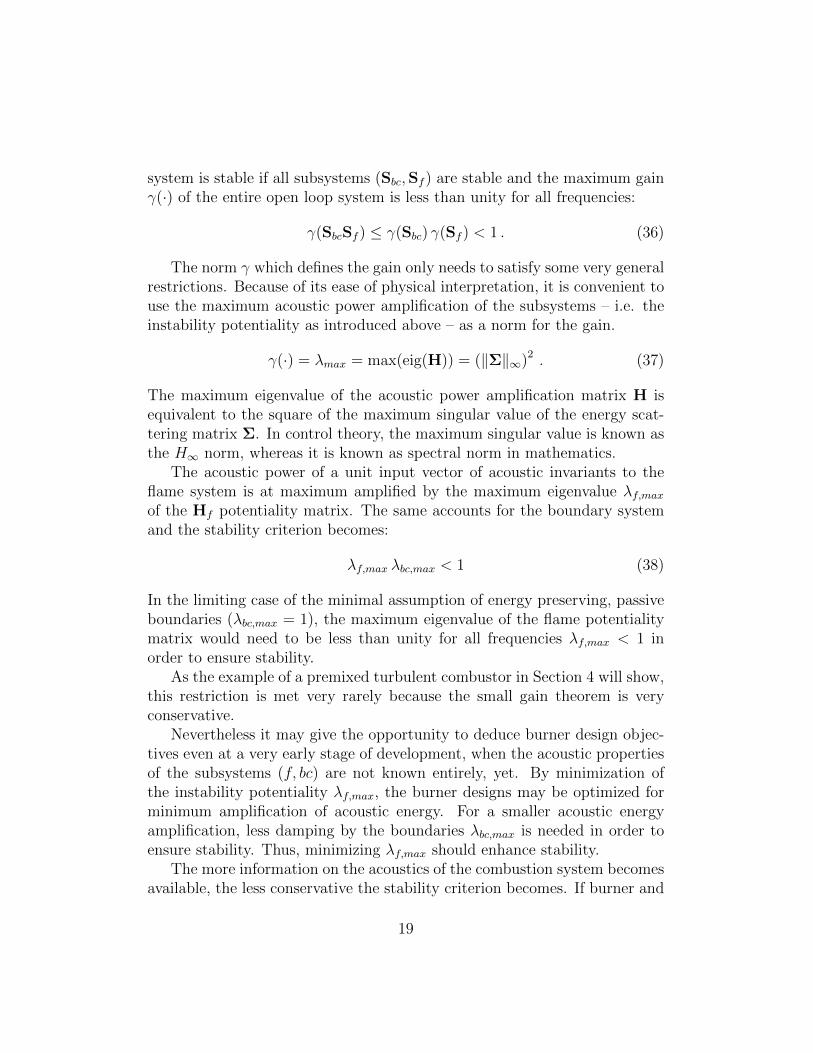
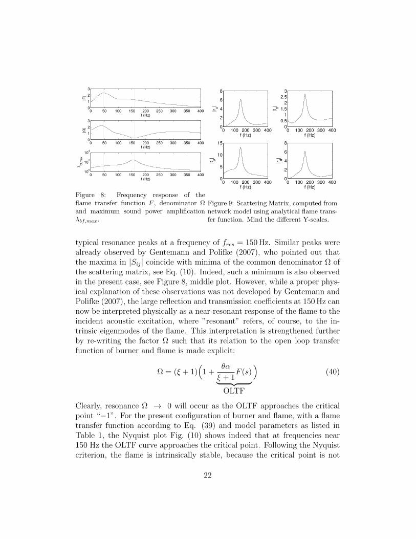
Previous studies conducted by Lawn and Polifke (2004), Schuermans et al.(2004) and Hirsch et al. (2005) have shown that this functional form ofthe flame transfer function in combination with the Rankine-Hugoniot jumpequations reproduces quite well the flame dynamics of typical turbulent pre-mix swirl burners. Furthermore, this form ensures the correct value |F | → 1in the limit of low frequencies Polifke and Lawn (2007). The parameters forthe TD1 flame considered in the present paper are also listed in Table 1.The gain |F | of the flame transfer function is shown in Figure 8 (top). It ex-hibits a characteristic local maximum in gain (“excess gain”) at a frequencyof around 50 Hz and then decays at higher frequencies.

Figure 9 depicts the absolute values of the coefficients of the scatteringmatrix Sbf of the acoustic system composed of burner and flame. The refer-ence positions of the scattering matrix upstream (u) and downstream (d) aremarked in the system sketch (Fig. 7). Remarkably, all four coefficients show

21

0 50 100 150 200 250 300 350 4000

1

2

3

f (Hz)

|F|

0 50 100 150 200 250 300 350 4000

1

2

3

f (Hz)

|Ω|

0 50 100 150 200 250 300 350 40010

0

102

104

f (Hz)

λb

f,m

ax

Figure 8: Frequency response of theflame transfer function F , denominator Ωand maximum sound power amplificationλbf,max.

0 100 200 300 4000

2

4

6

8

f (Hz)

|ru|

0 100 200 300 4000

0.5

1

1.5

2

2.5

3

f (Hz)

|td|

0 100 200 300 4000

5

10

15

f (Hz)

|tu|

0 100 200 300 4000

2

4

6

8

f (Hz)

|rd|

Figure 9: Scattering Matrix, computed fromnetwork model using analytical flame trans-fer function. Mind the different Y-scales.

typical resonance peaks at a frequency of fres = 150 Hz. Similar peaks werealready observed by Gentemann and Polifke (2007), who pointed out thatthe maxima in |Sij| coincide with minima of the common denominator Ω ofthe scattering matrix, see Eq. (10). Indeed, such a minimum is also observedin the present case, see Figure 8, middle plot. However, while a proper phys-ical explanation of these observations was not developed by Gentemann andPolifke (2007), the large reflection and transmission coefficients at 150 Hz cannow be interpreted physically as a near-resonant response of the flame to theincident acoustic excitation, where ”resonant” refers, of course, to the in-trinsic eigenmodes of the flame. This interpretation is strengthened furtherby re-writing the factor Ω such that its relation to the open loop transferfunction of burner and flame is made explicit:

Ω = (ξ + 1)(

1 +θα

ξ + 1F (s)︸ ︷︷ ︸

OLTF

)(40)

Clearly, resonance Ω → 0 will occur as the OLTF approaches the criticalpoint “−1”. For the present configuration of burner and flame, with a flametransfer function according to Eq. (39) and model parameters as listed inTable 1, the Nyquist plot Fig. (10) shows indeed that at frequencies near150 Hz the OLTF curve approaches the critical point. Following the Nyquistcriterion, the flame is intrinsically stable, because the critical point is not

22

−1 −0.5 0 0.5 1 1.5−1.4

−1.2

−1

−0.8

−0.6

−0.4

−0.2

0

0.2

0.4

0.6

Real Axis

Imag

inar

yA

xis

Pcrit

100

150

250

300

50

200

Figure 10: Nyquist plot of the open loop transfer function OLTF(s) of the burner model.

encircled by the OLTF.Correspondingly the maximum eigenvalue λbf,max of the acoustic power

amplification matrix Hbf peaks at 150 Hz (Figure 8). Energy generationλbf,max is larger than unity throughout the frequency range observed andpeaks at a value max(λbf,max) ≈ 315 (!). Thus, the flame is able to produceacoustic energy throughout all frequencies, and in particular so at 150 Hz.

Considering Figs. 8, 9 and 10 in the light of the arguments put forwardin Section 3.2, one concludes that the peaks in scattering matrix coefficients|ru|, |td|, |tu|, |rd| and in acoustic power amplification λmax are not due to ex-cess gain of the flame transfer function F (s), but due to the intrinsic feedbackloop and the associated resonance, manifested as the minimum in Ω at 150Hz.

Now we turn to the small gain theorem and its consequences for thepresent configuration. The boundary scattering Matrix Sbc is

Sbc =

(ru e

−s 2lu/cu 00 rd e

−s 2ld/cd

)(41)

When evaluating the quadratic form Hbc, the complex exponentials drop outand the maximum acoustic power amplification of the boundary is:

γ(Sbc) = λbc,max = max(r2u, r2d) (42)

23

ld

l u

−99.6

−59.4−59.4

−59.4

−59.4

−59.4

−59.4−59.4

−59.4−59.4

−19.2

0 0.5 1 1.5 20

0.5

1

1.5

2

Figure 11: Maximum growth rates of the modeled combustion system as a function ofnondimensionalized duct lengths up- and downstream for stable reflection factors ru =rd = 0.0563. Numbers indicate the values on isolines.

By evaluating the small gain stability criterion, a conservative limit for thereflection factors at the boundaries can be determined:

ru,d <

√1

max(λbf,max)≈ 0.0563 . (43)

For the given value of stable reflection factors ru = rd = 0.0563, a stabilitymap of the combustion system is shown in Figure 11. The maximum growthrate (smallest damping rate) is plotted as a function of the nondimension-alized lengths of the duct sections up- and downstream of the flame. Thelengths were varied between 0 and about two times the wave lengths insidethe respective ducts at the critical frequency of fres = 150 Hz l = l fres/c. Inagreement with the small gain stability criterion, we observe that the systemis stable for all parameters investigated with a maximum growth rate ob-served of −13.3. There are three resonant duct lengths up and downstreamand maximum growth rates are observed when both duct sections are tunedto be resonating. Apparently, a resonance of one duct section can be dampedby the other section if the corresponding length is set to a non resonatinglength.

24

5. Conclusion

The thermoacoustic stability of velocity sensitive premixed flames wasscrutinized. A causal representation of the acoustic-flow-flame-acoustic in-teractions revealed an intrinsic feedback mechanism: if an upstream velocitydisturbance induces a modulation of the heat release rate, an acoustic wavewill be generated that travels in the upstream direction, where it influencesin turn the acoustic velocity, such that a closed feedback loop results.

Even if the intrinsic eigenmodes of the flame, which result from thisfeedback loop are stable, the flame system has peaks in its acoustic energyamplification when excited at resonant frequencies. This was shown rigor-ously by evaluating the “instability potentiality” from a balance of acousticenergy across the flame. One obtains factors of maximum (as well as mini-mum) power amplification over all possible acoustic states. The relation ofmaximum power amplification to peaks in the scattering matrix coefficientsand the open loop transfer function of the internal flame dynamics was alsoelaborated.

Based on the acoustic power amplification, the small gain theorem wasintroduced and a corresponding energy-based stability criterion was formu-lated. Given passive boundaries, the gain – which is equivalent to the maxi-mum sound power amplification – must be less than unity for all frequenciesto ensure stability. The small gain theorem requires only minimal a prioriassumptions on upstream and downstream acoustic boundary conditions.

The concepts were exemplified first with a simplistic n-τ model and thenwith a flame transfer function that is representative of turbulent swirl burn-ers. It should be appreciated, however, that application of the ideas andmethods developed here are not restricted to these configurations. Acoustic-flow-flame-acoustic interactions that involve fluctuations of equivalence ratioor a pressure sensitive flame transfer function should in general also exhibitintrinsic feedback, with similar consequences for amplification of acousticpower and combustor dynamics as presented here. The causal mechanismsinvolved in a pressure sensitive response of the flame may be resonances of anacoustically ”soft” injection system as described by Huber and Polifke (2009),or autoignition (Zellhuber et al., 2014). The impact of those processes onthe flame intrinsic eigenmodes needs to be scrutinized and validated in futureresearch, which involves numerical and experimental investigations yet to bedone.

It is apparent that frequencies, where the acoustic power amplification of

25

the flame is very high, may be critical frequencies for the stability of a com-bustion system. More research and a validation with experiments regardingcritical burner frequencies are needed. First results have been presented byBomberg et al. (2014).

The small gain stability criterion is very conservative and therefore notimmediately useful for stability prediction in an applied context. Neverthe-less, it may be used as an optimization objective and comparison benchmarkfor combustor stability. Further studies to evaluate the effectiveness of thismethod are needed.

Furthermore, the small gain theorem is valid also for a large class ofnonlinear systems. Thus an extension and application to nonlinear flamemodels seems possible and will be the subject of future research.

6. Acknowledgements

The authors acknowledge financial support by the German Research Foun-dation DFG, project PO 710/12-1 and the Technische Universitat Munchen– Institute for Advanced Study, funded by the German Excellence Initiative.

Appendix A. Appendix: Dynamic System of the Flame Model( > O(M0))

The flame transfer function according to linearized Rankine-Hugoniotequations including effects of Mach numbers:[

p′

ρcd

u′d

]=

[ξ −θMd

−γθMu 1

][p′

ρcu

u′u

]+

[−Md

1

](TdTu− 1

)uuQ′

Q(A.1)

Transformation to scattering matrix representation including full equa-tions:[gufd

]=

1

ξ + θMd + γθMu + 1· (A.2)[

−ξ − (−θMd) + (−γθMu) + 1 22 ∗ (ξ − θMdγθMu) ξ + θMd − γθMu − 1

] [fugd

](A.3)

+

(TdTu− 1

)ξ + θMd + γθMu + 1

[Md + 1

−Md(γθMu + 1) + (ξ + θMd)

]F uu

fref − grefuref

(A.4)

26

Appendix B. Derivation of the Eigenvalues of the n-τ Flame Model

e−sτ = e−λτ (cos(−ωτ) + j sin(−ωτ)) = e−λτ (cos(ωτ)− j sin(ωτ)) = −1 + ξ

nθ(B.1)

Imaginary part (integers k introduced):

sin(ωτ) = 0 (B.2)

ωk =kπ

τ(B.3)

Real part:

e−λτ (cos(kπ

ττ)︸ ︷︷ ︸

=(−1)k

= −1 + ξ

nθ(B.4)

eλτ = (−1)k+1 nθ

1 + ξ(B.5)

λ and τ are real numbers, nθ1+ξ

> 0 thus solutions only exist for (−1)k+1 > 0

and the exponent needs to be even k + 1 = 2(z + 1) = 2z + 2 with

λk =1

τln((−1)2z+2︸ ︷︷ ︸

=1

nθ

1 + ξ) (B.6)

λz = λ =1

τln(

nθ

1 + ξ) (B.7)

The growth rate λ is the same for all eigenfrequencies. And eigenfrequenciesexist for:

ωz =(2z + 1)π

τ(B.8)

The complex eigenfrequencies sz of the inherent eigenmodes of the n-τ modelare:

sz = j(2z + 1)π

τ︸ ︷︷ ︸ωz

+1

τln

(nθ

1 + ξ

)︸ ︷︷ ︸

λ

. (B.9)

27

Appendix C. Characteristic Equation of the Flame Model

The characteristic equation Ω = 0:

F = −1 + ξ

θ(C.1)

Eliminating ξ using ideal gas law as it was done by Polifke (2011) (θ = ξ2−1):

ξ =√θ + 1 (C.2)

and the definition of θ

θ =TdTu− 1 (C.3)

in Equation (C.1)

F = −1 +√θ + 1

θ= −

1 +√

TdTu(√

TdTu

)2− 1

= − 1√TdTu− 1

. (C.4)

References

F. A. Williams, Combustion Theory, Addison-Wesley Publishing Company,2nd edition, 1985.

B. Lewis, G. von Elbe, Combustion, Flames, and Explosion of Gases, Aca-demic Press: New York, 3 edition, 1987.

P. Clavin, Prog. Energy Combust. Sci. 11 (1985) 1–59.

J. Buckmaster, Annual review of fluid mechanics 25 (1993) 21–53.

M. Matalon, Annu. Rev. Fluid Mech. 39 (2007) 163–191.

M. Kroner, J. Fritz, T. Sattelmayer, Journal of Engineering for Gas Turbinesand Power 125 (2003) 693–700.

S. K. Aggarwal, Progress in Energy and Combustion Science 35 (2009) 528– 570.

D. E. Cavaliere, J. Kariuki, E. Mastorakos, Flow, Turbulence and Combus-tion 91 (2013) 347–372.

28

J. W. S. Rayleigh, Nature 18 (1878) 319–321.

J. J. Keller, AIAA Journal 33 (1995) 2280–2287.

T. Lieuwen, V. Yang (Eds.), Combustion Instabilities in Gas Turbine En-gines: Operational Experience, Fundamental Mechanisms, and Modeling,number ISBN 156347669X in Progress in Astronautics and Aeronautics,AIAA, 2006.

W. C. Strahle, J. of Fluid Mech. 49 (1971) 399–414.

A. Dowling, Journal of Sound and Vibration 180 (1995) 557–581.

M. Hoeijmakers, V. Kornilov, I. Lopez Arteaga, P. de Goey, H. Nijmeijer,Combust. and Flame (2014).

M. Hoeijmakers, I. Lopez Arteaga, V. Kornilov, H. Nijmeijer, P. de Goey, in:Proceedings of the European Combustion Meeting, Lund,Sweden.

S. Bomberg, T. Emmert, W. Polifke, in: 35th International Symposium onCombustion, The Combustion Institute, San Franciso, CA, USA.

N. Noiray, D. Durox, T. Schuller, S. Candel, Proceedings of the CombustionInstitute 31 (2007) 1283–1290.

T. Komarek, W. Polifke, J. Eng. Gas Turbines Power 132 (2010) 061503–1,7.

Y. Auregan, R. Starobinski, Acta Acustica united with Acustica 85 (1999)5–5.

W. Polifke, in: European Combustion Meeting, ECM2011, British Section ofthe Combustion Institute, Cardiff, UK.

G. Zames, Automatic Control, IEEE Transactions on 11 (1966) 228–238.

D. L. Straub, G. A. Richards, Int. Gas Turbine \& Aeroengine Congress \&Exhibition, ASME, 1999.

P. Palies, D. Durox, T. Schuller, S. Candel, Journal of Fluid Mechanics 672(2011) 545–569.

R. S. Blumenthal, P. Subramanian, R. Sujith, W. Polifke, Combustion andFlame 160 (2013) 1215–1224.

29

S. Jaensch, T. Emmert, W. Polifke, in: Proceedings of ASME Turbo Expo2014, GT2014-27034, Dusseldorf, Germany.

M. L. Munjal, Acoustics of ducts and mufflers, John Wiley & Sons, 1987.

W. Polifke, in: C. Schram (Ed.), Advances in Aero-Acoustics and Thermo-Acoustics, Van Karman Institute for Fluid Dynamics., Rhode-St-Genese,Belgium, 2010.

L. Tay-Wo-Chong, S. Bomberg, A. Ulhaq, T. Komarek, W. Polifke, Journalof Engineering for Gas Turbines and Power 134 (2012) 021502–1–8.

B. T. Chu, volume 4, pp. 603–612.

J. Kopitz, W. Polifke, J. Comp. Phys 227 (2008) 6754–6778.

T. Schuller, D. Durox, S. Candel, Combust. and Flame 134 (2003) 21–34.

C. O. Paschereit, B. B. H. Schuermans, W. Polifke, O. Mattson, J. Eng.Gas Turbines Power 124 (2002) 239–247. Originally published as ASME99-GT-133.

W. Polifke, A. M. G. Gentemann, Int. J. of Acoustics and Vibration 9 (2004)139–148.

A. Gentemann, W. Polifke, in: Int’l Gas Turbine and Aeroengine Congress& Exposition, ASME GT2007-27238, Montreal, Quebec, Canada.

W. Polifke, C. J. Lawn, Combust. Flame 151 (2007) 437–451.

H. Nyquist, Bell System Technical Journal (1932) 1–24.

B. T. Chu, Acta Mechanica (1964) 215–234.

H. R. Cantrell, R. W. Hart, F. T. McClure, AIAA 2 (1964) 1100–1105.

C. L. Morfey, J. Sound Vib. 14 (1971) 159–170.

M. K. Myers, Journal of Fluid Mechanics 226 (1991) 383–400.

A. Giauque, T. Poinsot, M. Brear, F. Nicoud, in: Proc. of the SummerProgram, p. 285–297.

30

M. J. Brear, F. Nicoud, M. Talei, A. Giauque, E. R. Hawkes, Journal of FluidMechanics 707 (2012) 53–73.

K. J. George, R. Sujith, Journal of Sound and Vibration 331 (2012) 1552–1566.

A. M. Lyapunov, A. T. Fuller, The general problem of the stability of motion,Tayor & Francis, London ; Washington, DC, 1992.

N. Rouche, P. Habets, M. LaLoy, Stability theory by Liapunov’s directmethod, number 22 in Applied mathematical sciences, Springer-Verlag,New York, 1977.

P. Subramanian, R. I. Sujith, Journal of Fluid Mechanics 679 (2011) 315–342.

R. S. Blumenthal, A. K. Tangirala, R. Sujith, W. Polifke, in: n3l Workshop onNon-Normal and Nonlinear Effects in Aero- and Thermoacoustics, Munich,Germany.

K. Wieczorek, C. Sensiau, W. Polifke, F. Nicoud, Phys. Fluids 23 (2011)107013–1 – 14.

A. P. Dowling, J. E. Ffowcs Williams, Sound and Sources of Sound, EllisHorwood Limited, 1983.

W. Polifke, A. Fischer, T. Sattelmayer, J. Eng. Gas Turbines Power 125(2003) 20–27. Originally published as ASME 2001-GT-35.

A. M. G. Gentemann, C. Hirsch, K. Kunze, F. Kiesewetter, T. Sattelmayer,W. Polifke, in: Int’l Gas Turbine and Aeroengine Congress & Exposition,ASME GT-2004-53776, Vienna, Austria.

C. J. Lawn, W. Polifke, Comb. Sci. Tech. 176 (2004) 1359 – 1390.

B. Schuermans, V. Bellucci, F. Guethe, F. Meili, P. Flohr, O. Paschereit.

C. Hirsch, D. Fanaca, P. Reddy, W. Polifke, T. Sattelmayer, in: Int’l GasTurbine and Aeroengine Congress & Exposition, ASME GT2005-68195 ,Reno, NV, U.S.A.

A. Huber, W. Polifke, Int. J. Spray Comb. Dynamics 1 (2009) 199–250.

M. Zellhuber, B. Schuermans, W. Polifke, Combustion Theory and Modelling18 (2014) 1–31.

31