1

Flatland in flames: a two-dimensional canopy fire propagation 1

model 2

3

4

5

Authors: 6

James Dickinson1,2, Andrew Robinson3, Paul Gessler4, Richy Harrod2, Alistair Smith5 7

8

9

Keywords: canopy bulk density, foliar biomass per unit area, fba, crown fire, equivalence 10

test11

1 Corresponding author: jddickinson@fs.fed.us 2 Fire Ecologist, USDA Forest Service, Okanogan-Wenatchee National Forests, Wenatchee, Washington,United States 3 Senior Lecturer of Applied Statistics, University of Melbourne, Melbourne, Victoria, Australia 4 Associate Professor of Remote Sensing & Spatial Ecology, University of Idaho, Moscow, Idaho, United States 5 Assistant Professor of Forest Measurements, University of Idaho, Moscow, Idaho, United States

2

Non-specialist summary: 1

Canopy fire modeling is based largely upon the use of canopy bulk density, a three-2

dimensional crown measure, as a fuel metric. We propose and test a model that relies on a 3

two-dimensional crown measure, which is simpler to conceptualize and easier to obtain 4

remotely. We compare the model with its three-dimensional equivalent, with two 5

contemporary fuel inputs methods. We find that the alternative fuel metric provides 6

statistically equivalent modeled outputs of canopy fire propagation 2626 FIA plots. 7

Abstract: 8

Canopy bulk density (CBD) is widely used as metric for quantifying the fuel available 9

for combustion in canopy fire and as an input to Van Wagner’s (1977) model for 10

estimating the critical rate of spread necessary to sustain active canopy fire. We propose a 11

modification of Van Wagner’s approach to use foliar biomass per unit area (FBA) as the 12

fuel input. Unlike CBD, FBA does not require incorporation of the vertical distribution of 13

the fuel, so it is readily measurable (and estimable) by foresters, tree physiologists and fire 14

managers. The new model provides a more consistent explanation for Van Wagner’s 15

original observations. We test our modified model for equivalence to the original Van 16

Wagner model, incorporating two contemporary techniques for calculating CBD. We find 17

that the modified model is equivalent to the original model using the CBD method 18

incorporated into the Fire and Fuels Extension to the Forest Vegetation Simulator, but not 19

the CBD method of Cruz et al. (2003). Although equivalent (at α = .10, N = 2626) the 20

FBA input produced a mean difference of 0.010 ms-1 less for the critical rate of spread 21

necessary to sustain canopy fire. The adoption of FBA as a fuel input may allow for 22

consistent fuel quantifications that are less influenced by the highly varied canopy structure 23

3

of forested stands than CBD, and could facilitate remotely sensed canopy fuel 1

quantification. 2

Introduction: 3

Canopy fire is a challenge for the accurate modeling of fire spread because 4

quantification of the canopy fuel stratum is difficult (Cruz et al. 2003, Keane et al. 2005). 5

Particular difficulty arises because canopy fires can exist in either ‘passive’ or ‘active’ 6

modes. In passive canopy fires, individual trees or groups of individuals ignite and burn 7

from the bottom to the top of the crown, resulting in mixed impacts on the environment 8

(Ryan and Noste 1983). In active canopy fires the combustion propagates as a solid wall of 9

flame through a landscape filled with trees, in conjunction with a surface fire (Van Wagner 10

1977). In addition, this combination of active canopy and surface fire often burns at high 11

intensity having significant impact on soils, vegetation, and wildlife habitat (Grier 1975, 12

Ryan and Noste 1983, Romme 1995, Haggard and Gaines 2001). Such fires may exhibit 13

flame lengths exceeding 30-m with rates of spread exceeding 50 m min-1 (Stocks et al. 14

2004). Active canopy fire also poses great risk to fire personnel, the public, and private 15

property (Scott 1998, Clark et al. 1999, Scott and Reinhardt 2001). 16

For these reasons, fire managers seek to implement preventative treatment of forested 17

landscapes capable of sustaining active canopy fires (Hof and Omi 2003, Scott 2003, 18

Peterson et al. 2005). They also wish to predict and understand the behavior of these fires 19

(Stocks et al. 2004). Such applications require knowledge of the minimal conditions 20

required to sustain a canopy fire to support mitigation treatments and assessment of hazard 21

to fire personnel during active fires. 22

4

Most fire planning tools and spatially explicit fire models depend upon Van Wagner’s 1

(1977) model (we refer to this model as VWcbd) to characterize the minimum conditions 2

necessary to sustain active canopy fire (Keane et al. 2000, Scott and Reinhardt 2001, 3

Finney et al. 2003, Reinhardt and Crookston 2003, Finney 2004). VWcbd relies on a 4

three-dimensional metric of available canopy fuel for combustion called canopy bulk 5

density (CBD), which other research has attempted to quantify (Keane et al. 2000, Fule et 6

al. 2001, Hummel and Agee 2003, Riano et al. 2003, Gray and Reinhardt 2003, Perry et al. 7

2004, Riano et al. 2004, Falkowski et al. 2005, Peterson et al. 2005, Keane et al. 2005). 8

However, the dominant sources of information, and frameworks within which fire 9

management decisions are made, are inherently two dimensional. 10

The ability to field test, calibrate, refine, or even observe the efficacy of the VWcbd 11

estimates has been limited mostly because of the inherent difficulties of obtaining the 12

three-dimensional CBD input. Scott and Reinhardt (2005) report nearly 1000 person-hours 13

required to physically measure several canopy biomass variables (including their vertical 14

distribution) to calculate canopy fuel CBD for a single 10m radius plot. This expense to 15

physically measure the volume space used in CBD calculations has made it difficult to 16

assess the utility of the model as put forth by Van Wagner (1977) (Keane et al. 2005). 17

We develop VWfba, a modified version of VWcbd, that uses foliar biomass per unit 18

area (FBA) as a fuel input. Use of FBA may allow for consistent fuel quantifications that 19

are less influenced than CBD by highly varied canopy structure common in forested 20

stands. We compare VWfba with the existing VWcbd, using two different CBD 21

estimation methods, to determine if FBA can be used with confidence in existing fire 22

modeling applications with minor modification. The relationship of FBA to traditional 23

5

forest mensuration, forest physiology, and remote sensing variables should make canopy 1

fuel estimates more consistent and readily attainable for forest manager concerned with 2

canopy fire propagation and fuels management. 3

Crown fire defined: 4

Van Wagner (1977) described a conceptual canopy fire model using “a stationary wall 5

of flame with a conveyor belt carrying fuel into the flame”. The conveyor belt must 6

maintain a rate greater than minimum critical rate of spread (cROS) in order to deliver a 7

sufficient quantity of combustible fuel per unit time to maintain the wall of flame in the 8

canopy space (Van Wagner 1977). 9

Van Wagner modeled canopy fire interactions for fuel, flame front rate of spread, and 10

the minimum fireline intensity necessary to maintain canopy fire in a fashion similar to 11

Byram’s (1959) index. This surface fire index relates fireline intensity, the rate of spread of 12

a flame front, and the quantity of combusted fuel (Byram 1959, Scott and Reinhardt 2001). 13

By representing the flame front as a line moving at some rate across a plane of 14

homogenously distributed fuel mass (multiplied by a constant heat yield) the result is a 15

fireline intensity that is the product of the rate of flame movement and the homogeneous 16

fuel (Byram 1959). Like Byram’s (1959) index, the VWcbd assumes a homogeneously 17

distributed fuelbed, albeit through a volume rather than across an area (Van Wagner 1977). 18

The assumption of a homogeneous fuel bed with a constant heat yield per unit of fuel 19

makes VWcbd identical to Byram’s (1959) index in form. 20

The Van Wagner (1977) model differs only in form by its calibration to the minimal 21

conditions necessary for active canopy fire to persist. Van Wagner assumed that the fuel 22

present in a stand would have a constant heat of ignition (per unit mass), and thus avoided 23

6

the necessity of calculating the energy in the propagating heat flux. This changed the 1

crucial element to a simple argument that relates only the critical quantity of fuel 2

consumed per unit time required for flame maintenance, divided by the available fuel 3

quantity (Eq. 1). The result of this equation is the critical rate of spread (cROS, represented 4

by ‘Ro’ in Eq. 1) required for the fire to consume the available fuel (‘d’) such that the 5

critical mass flow rate (‘So’) is satisfied. 6

Ro = dSo (Van Wagner 1977) (1) 7

Where: Ro : cROS for active canopy fire (m s-1) 8

So : critical mass flow rate for canopy fire, (0.05 kg m-2 s-1) 9

d: foliar (canopy) bulk density (kg m-3) 10

11

Van Wagner’s definition of canopy fire as a wall of continuous flame from bottom to 12

top of the canopy must be met to satisfy the implicit assumption that canopy fire has 13

initiated (Van Wagner 1977; Scott and Reinhardt 2001). The use of a single value to 14

represent a distribution of fuel through the canopy space removes any influence that the 15

vertical distribution of fuel may have upon canopy fire, requiring a second assumption that 16

horizontal canopy fire propagation occurs regardless of the vertical distribution of the 17

fuel. The quotient resulting from the division of the available fuel by volume (the 18

definition of CBD) is simply a fraction of the total fuel load (the sum of which is still 19

available for combustion) and does not relate to the effect that the vertical distribution may 20

(or may not) have on canopy fire. 21

A properly calibrated model that uses a fuel metric with no vertical distribution 22

component does not preclude the use of vertical distribution as a parameter in the model. 23

7

The fuel input to such a model would be useable at a range of scales depending only upon 1

the method used to calculate the available canopy fuel. 2

We assume that the Van Wagner (1977) model appropriately relates the basic 3

properties necessary to describe the lower boundary conditions required for active canopy 4

fire combustion. (Namely, that an active canopy fire spreading between two points on the 5

landscape must consume a minimum quantity of fuel per unit time in order to persist as a 6

canopy fire.) The quantification of fuel is vital to a model of the combustion process. 7

However, we argue that the quantification need not incorporate the vertical distribution 8

into the fuel metric as traditional canopy fuel methodologies have done. 9

We use Van Wagner’s (1977) published data to recalibrate the model for use with FBA 10

in place of the standard CBD input. The VWcbd and the VWfba models are applied to a 11

region-wide non-spatial FIA database and an equivalence test is used to compare the 12

estimates of cROS from the VWcbd and VWfba models. 13

Methods 14

In this section we introduce two methods used to calculate the fuel input necessary for 15

VWcbd. We compared only the Fire and Fuels Extension to the Forest Vegetation System 16

(FFE) (Reinhardt and Crookston 2003) and Cruz et al. (2003) methods because they 17

represent the two distinct approaches to estimating CBD. We then modify the existing 18

VWcbd for the use of foliar biomass to create the VWfba model. Finally, we introduce our 19

data and the statistical methods used to test the equivalence of the VWcbd and VWfba. 20

21

8

Summary of CBD methods: 1

The widespread use of the complex FFE method by US federal land managers and 2

researchers (Hummel and Agee 2003, Andersen et al. 2005, Perry et al. 2004, Falkowski et 3

al. 2005, Peterson et al. 2005) is facilitated by its implementation in the Fire and Fuels 4

Extension to the Forest Vegetation Simulator (FFE-FVS) computer software (Reinhardt 5

and Crookston 2003) and the proprietary Fire Management Analyst Plus suite of computer 6

software (FPS 2001). 7

When applied to a stand inventory list, FFE calculates the foliar biomass assuming a 8

constant density of foliar biomass through the length of the individual tree-crown space. 9

FFE calculates the amount of biomass contained in every vertical 0.3048 meter (1-foot) of 10

the volume space for each tree (Scott and Reinhardt 2001). Finally, the foliar biomass for 11

all individuals in the stand is summed within each vertical 0.3048 meter above the ground 12

and is plotted (see Fig. 1). This represents stand biomass (kg m-2) distributed by height 13

above ground (m), as a sum of all individual trees (i.e. vertical distribution of foliage 14

within the canopy space) (Sando and Wick 1972). 15

FFE calculates the maximum 0.3048 m (1 ft) increment of a 3.96 m (13-foot) running 16

mean applied to the vertical profile of foliar biomass (see Fig. 1)(Reinhardt and Crookston 17

2003). This produces an effective CBD value that differs from the traditional CBD 18

definition (Scott and Reinhardt 2001). Effective CBD provides a value that is the 19

maximum of a running average (Fig 1) and represents the greatest average fuel value, 20

presumed to be the least resistant stratum for canopy fire propagation through a stand 21

(Scott and Reinhardt 2001). Despite the lack of direct correspondence to the CBD 22

definition, effective CBD is frequently used as input to VWcbd. 23

9

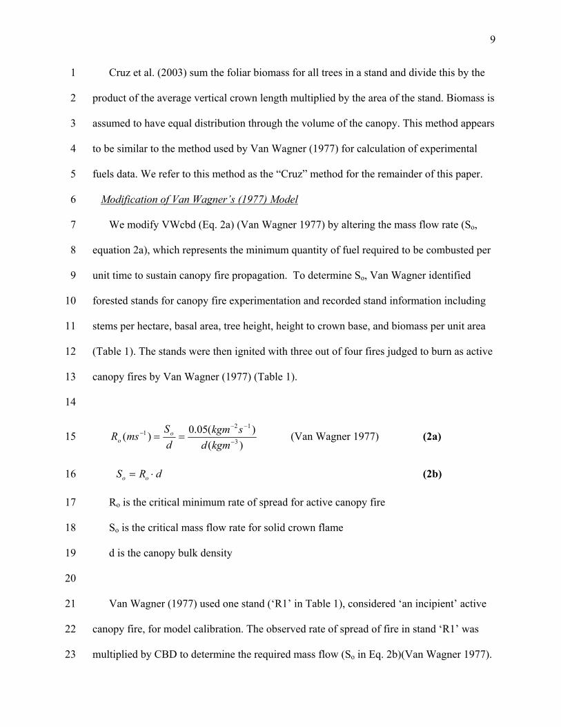
Cruz et al. (2003) sum the foliar biomass for all trees in a stand and divide this by the 1

product of the average vertical crown length multiplied by the area of the stand. Biomass is 2

assumed to have equal distribution through the volume of the canopy. This method appears 3

to be similar to the method used by Van Wagner (1977) for calculation of experimental 4

fuels data. We refer to this method as the “Cruz” method for the remainder of this paper. 5

Modification of Van Wagner’s (1977) Model 6

We modify VWcbd (Eq. 2a) (Van Wagner 1977) by altering the mass flow rate (So, 7

equation 2a), which represents the minimum quantity of fuel required to be combusted per 8

unit time to sustain canopy fire propagation. To determine So, Van Wagner identified 9

forested stands for canopy fire experimentation and recorded stand information including 10

stems per hectare, basal area, tree height, height to crown base, and biomass per unit area 11

(Table 1). The stands were then ignited with three out of four fires judged to burn as active 12

canopy fires by Van Wagner (1977) (Table 1). 13

14

)()(05.0)( 3

121

−

−−− ==

kgmdskgm

dS

msR oo (Van Wagner 1977) (2a) 15

dRS oo ⋅= (2b) 16

Ro is the critical minimum rate of spread for active canopy fire 17

So is the critical mass flow rate for solid crown flame 18

d is the canopy bulk density 19

20

Van Wagner (1977) used one stand (‘R1’ in Table 1), considered ‘an incipient’ active 21

canopy fire, for model calibration. The observed rate of spread of fire in stand ‘R1’ was 22

multiplied by CBD to determine the required mass flow (So in Eq. 2b)(Van Wagner 1977). 23

10

It was apparent that this resulting value was less than necessary for active canopy fire so 1

Van Wagner set So at a constant value slightly greater (0.05 kgm-2s-1) (VanWagner 1977). 2

This established the minimum mass flow value necessary because a slower fuel 3

consumption rate would result in fire behavior similar to the incipient canopy fire behavior 4

of ‘R1’ (Van Wagner 1977). 5

For VWfba, we divide Van Wagner’s value of So= 0.05 kgm-2s-1 by the CBD for stand 6

‘R1’ (0.23 kgm-3) (Eq. 3a). The result is a cROS of 0.217 ms-1 for stand ‘R1’. The cROS 7

is multiplied by the FBA (foliar biomass per unit area, Table 1) of stand ‘R1’ resulting in a 8

product of 0.39 kgm-2s-1 (Eq. 3b) giving the predictive equivalent to Van Wagner’s 9

published value using CBD of So = 0.05 kgm-2s-1 (Eq. 3c). 10

11

)(217.0)(23.0)(05.0 1312 −−−− =÷ mskgmskgm (3a) 12

)(39.0)(80.1)(217.0 1121 −−−− =∗ skgmkgmms (3b) 13

)(80.1)(39.0)(217.0

)(23.0)(05.0

2

111

3

12

−

−−−

−

−−

==kgm

skgmmskgm

skgm (3c) 14

15

The final form of the VWfba model is then: 16

17

)()(39.0)( 2

111

−

−−− =

kgmdskgmmsRo (4) 18

After recalibration of So, the VWfba model was applied to the rest of the data provided 19

by Van Wagner (1977) (Fig. 2). With exception of the calibration fire ‘R1’, all of these 20

fires were observed canopy fires. A satisfactory model will have a predicted cROS that is 21

exceeded by the observed rate of spread. Inputs for these predictions were taken from Van 22

11

Wagner’s published data. The method of cbd estimation for input to the original VW 1

model is unspecified. The published foliar biomass per unit ground area for these stands is 2

used as FBA input to the VWfba model. The VWfba and VWcbd (where FBA and cbd 3

inputs are provided in Van Wagner (1977)) models provide comparable predictions of 4

cROS (Fig. 2). Additionally, VWfba identifies stand “GLB Active” as exceeding the 5

cROS, and correctly classifies it as an active canopy fire, whilst VWcbd does not (Fig. 2). 6

Sample data 7

We use a database of 2626 Forest Inventory and Analysis (FIA) plots collected from 8

the Inland Northwest region of the United States (Gillespie 1999, UIFBL 2006). FIA 9

routinely collects data on trees, saplings, and seedlings at each plot; however, we selected 10

only trees at least 7.56 cm (3”) in diameter at breast height (1.37 meters) (USDA Forest 11

Service 1990). Each of the 40,000 tree records in this database include the variables of tree 12

diameter, height, percent live crown ratio, species, and the tree expansion factor (number 13

of trees per hectare that record represents) and plot level variables (e.g. elevation, habitat 14

type, aspect, and slope. 15

Statistical analysis 16

Model validation is poorly served by traditional frequentist null hypothesis significance 17

testing (NHST), because NHST requires that the null hypothesis be stated such that the two 18

models are not significantly different (Wellek 2003). The ability to demonstrate similarity 19

rather than difference based on probability arises by changing the null hypothesis from one 20

of similarity; to one stating that dissimilarity exists, and is called equivalence testing 21

(Wellek 2003; Robinson and Froese 2004). Though the biomedical industry has long used 22

equivalence tests to show that two samples are statistically similar, equivalence tests have 23

12

not been widely applied to ecological modeling (Wellek 2003, Robinson and Froese 2004). 1

Robinson and Froese (2004) use equivalence tests to validate model predictions of the 2

diameter growth model contained within the Forest Vegetation Simulator. 3

This test requires that a region of indifference (ε), or a range of difference that is of 4

negligible concern, be established (Robinson and Froese 2004). That is, a range of 5

difference between sample metrics that is insignificant in practical application (Wellek 6

2003). After establishing a region of indifference, two separate trials of a one sided t-test 7

on the difference between samples is carried out, one for differences greater than the test 8

statistic, and one trial for differences less than the test statistic (Robinson and Froese 9

2004). This method is called a ‘two-one-sided t-test’ (TOST) and like a regular t-test, this 10

test gains power as the sample size increases (Robinson and Froese 2004). 11

The null hypothesis of dissimilarity is rejected if the range of indifference overlaps into 12

the rejection region for a one-tailed 95% confidence interval of the mean of the differences 13

( diffba xxx =− ) (Robinson and Froese 2004). The mathematics behind equivalence testing 14

do not make p-values practical, so we use both a strict (small) and liberal (large) range of 15

indifference to bracket our confidence in the hypothesis test (Wellek 2003). 16

These ranges of indifference bracket our confidence based not on probability, but on a 17

judgment of how large the difference could be for the models to still be considered 18

equivalent. In this paper, we choose a strict range of indifference such that | diffx ± ε| < 19

0.138 m s-1 (± 0.50 kph) for cROS, while the liberal range of indifference was established 20

such | diffx ± ε| < 0.278 m s-1 (± 1.0 kph). The values were chosen as being insignificant 21

ranges of difference from both a management and a modeling standpoint. We use a one 22

13

sided type I error rate of 5% (α= .05), which translates to two times a one-sided α (2 x .05 1

= .10) for our TOST test of equivalence. 2

Results 3

Our data exhibit light tails, relative to the normal distribution, however our large sample 4

size lends resistance to departures from normality (Ramsey and Schafer 2002). To verify that 5

outliers were not affecting the results we removed obvious outliers and reran the TOST. In 6

each comparison of models, removing the outliers made the minimum region of indifference 7

smaller. Hence, the null hypothesis was more clearly rejected with the outliers removed in 8

each comparison and we present our results with all data represented. 9

The mean of the differences between cROS for FIA plots using VWcbd-FFE and VWfba 10

is only 0.010 ms-1 (Table 2). Despite a comparatively large standard deviation the null 11

hypothesis of dissimilarity is rejected. The sum of the minimum range of indifference and 12

the mean of the difference (0.010 ± 0.027 ms-1) is substantially less than the conservative 13

range of indifference lending strong evidence (in lieu of a p-value) that the rejection of the 14

null hypothesis is justified (Table 2). 15

These same patterns are repeated for the comparison of VWcbd-Cruz and VWcbd-FFE, 16

though the mean of the difference is larger than the previous comparison (0.050 ms-1) (Table 17

2). Again, the sum of the difference and the minimum range of indifference (0.050 ± 0.066 18

ms-1) is well within the predefined conservative range of indifference leading to a 19

comfortable rejection of the null hypothesis. In the final comparison between VWcbd-Cruz 20

and VWfba the mean of differences is larger than any of the previous comparisons (0.060 21

ms-1) (Table 2). The sum of this large bias between the models and corresponding large 22

minimum region of indifference (0.060 ± 0.086 ms-1) does not allow a rejection of the null 23

14

hypothesis of dissimilarity under the conservative scenario, though it is still rejected at the 1

liberal range. In all but one of these comparisons we reject the null hypothesis of 2

dissimilarity. 3

Discussion 4

The VWfba provides the lowest estimate of cROS between these three methods. These 5

differences, 0.010 ms-1 and 0.060 ms-1, are interpreted to mean that on average the VWfba 6

model estimates the cROS necessary to sustain canopy fire to be less than the cROS 7

predicted by the VWcbd-FFE and VWcbd-Cruz respectively. This result is likely due the 8

VWfba utilization of all available fuel and not some fraction of the available fuel which 9

means that the cROS does not need to be as high as the case where less fuel is available. 10

The VWcbd and VWfba estimates for the regional FIA data (n=2676) are equivalent to 11

one another well within acceptable ranges of indifference established for these tests. We 12

demonstrate that VWfba is equivalent to VWcbd in the Inland Northwest when the 13

sampling design of FIA is followed and the data used to describe a 0.40 hectare (1 acre) 14

stand. Based on our analysis of comprehensive FIA data, we conclude that the use of 15

VWfba is a reasonable alternative to VWcbd, in particular when compared to VWcbd-ffe. 16

Like CBD estimates, FBA is limited by the accuracy of the technologies used to 17

estimate foliar biomass (total available fuel). However, CBD methods have the added 18

difficulty of measuring the necessary volume. The ability to field test, calibrate, refine, or 19

even observe the efficacy of the VWcbd estimates has been limited mostly because of the 20

complex, more difficult measurement of the CBD input. 21

In summary, the adoption of VWfba may allow for consistent fuel quantifications that 22

are less influenced by the highly varied canopy structure of forested stands than CBD. 23

15

Furthermore, data collection for VWfba should be much cheaper, and easier over large 1

scales, if it can be related to remotely sensed measurements. The VWfba recalibration of 2

Van Wagner’s (1977) model provides statistically equivalent estimates and is consistent 3

with the original field observations of Van Wagner (1977). 4

The VWfba model proposed here only quantifies the fuel conditions necessary to 5

sustain canopy fire between two points on the landscape with the intention of matching the 6

performance of the original Van Wagner (1977) model. This model does not require 7

knowledge about the vertical distribution of fuel, only that enough fuel exists between two 8

points to sustain canopy fire. Future work with the VWfba model may require a coefficient 9

to describe vertical distribution or a number of other parameters, but these coefficients will 10

be independent of the combustible biomass estimate. This approach leads to a more subtle 11

refinement of the model output independent of the quantity of fuel that is truly available to 12

the advancing canopy fire. 13

The VWfba model should next be applied to a variety of case studies where estimates 14

of foliar biomass can be obtained for observed canopy fires. An example of this sort of 15

validation could be the acquisition of LANDSAT imagery over an area subsequent to a 16

canopy fire. Using estimates of foliar biomass derived from leaf area index (LAI) and 17

specific leaf area (SLA), the resulting VWfba prediction could be compared to fire 18

behavior observations from that fire. This type of field validation removes the necessity of 19

estimating the probable fire spread direction and then placing fuel sampling personnel 20

directly in the path of impending canopy fires, allowing the required fire observations to be 21

conducted from a safe distance. Given the lack of literature suggesting that the use of 22

VWcbd adequately provides estimates of the cROS threshold we would not necessarily 23

16

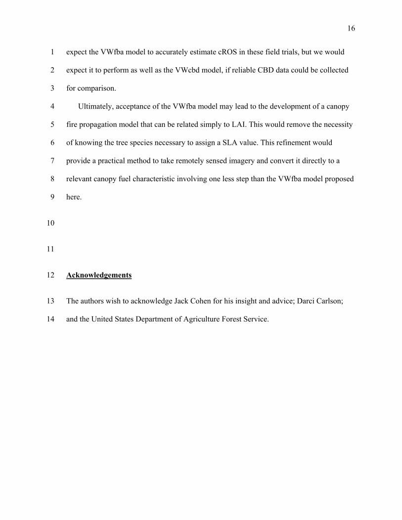
expect the VWfba model to accurately estimate cROS in these field trials, but we would 1

expect it to perform as well as the VWcbd model, if reliable CBD data could be collected 2

for comparison. 3

Ultimately, acceptance of the VWfba model may lead to the development of a canopy 4

fire propagation model that can be related simply to LAI. This would remove the necessity 5

of knowing the tree species necessary to assign a SLA value. This refinement would 6

provide a practical method to take remotely sensed imagery and convert it directly to a 7

relevant canopy fuel characteristic involving one less step than the VWfba model proposed 8

here. 9

10

11

Acknowledgements 12

The authors wish to acknowledge Jack Cohen for his insight and advice; Darci Carlson; 13

and the United States Department of Agriculture Forest Service.14

17

References: 1

Andersen HE, McGaughey RJ, Reutebuch SE (2005) Estimating forest canopy fuel 2

parameters using LIDAR data. Remote Sensing of Environment 94, 441 – 449. 3

4

Byram GM, 1959. Combustion of Forest Fuels. In: Forest Fire Control and Use, 1st 5

edition. New York: McGraw-Hill. Chapter 3, 61-89. 6

7

Clark TL, Radke L, Coen J, Middleton D (1999) Analysis of small-scale convective 8

dynamics in a crown fire using infrared video camera imagery. Journal of Applied 9

Meteorology 38, 1401 – 1420. 10

11

Cruz MG, Alexander ME, Wakimoto RH (2003) Assessing canopy fuel stratum 12

characteristics in crown fire prone fuel types of western North America. International 13

Journal of Wildland Fire 2003(12), 39 – 50. 14

15

Falkowski M, Gessler PE, Morgan P, Hudak AT, Smith AM. 2005. Characterizing and 16

mapping forest fire fuels using ASTER imagery and gradient modeling. Forest Ecology 17

and Management 217, 129 – 146. 18

19

Finney MA. (Revised 2004) FARSITE: Fire Area Simulator-model development and 20

evaluation. USDA Forest Service, Rocky Mountain Research Station Research Paper 21

RMRS-RP-4. (Ogden, UT) 47 pp. 22

18

Finney MA, Britten S, Seli R (2003) FlamMap2 Beta Version 3.0.1. Fire Sciences Lab and 1

Systems for Environmental Management, Missoula MT. 2

3

FPS (2001) Fire program solutions, LLC. Acquired from: http://www.fireps.com/ 4

Accessed: Tuesday, April 05, 2005 5

6

Fule PZ, Waltz AE, Covington WW, Heinlein TA (2001) Measuring forest restoration 7

effectiveness in reducing hazardous fuels. Journal of Forestry November, 24 – 29. 8

9

Gillespie, A.J.R. (1999) Rationale for a National Annual Forest Inventory Program. 10

Journal of Forestry December, 97(12), pp. 16-20. 11

12

Gray KL, Reinhardt ED (2003) Analysis of algorithms for predicting canopy fuel. 2nd 13

International Wildland Fire Ecology and Fire Management Congress and 5th Symposium 14

on Fire and Forest Meteorology. Orlando FL, Nov. 16-20, 2003. 15

16

Grier CC (1975) Wildfire effects on nutrient distribution and leaching in a coniferous 17

ecosystem. Canadian Journal of Forest Research 5, 599 – 607. 18

19

Haggard M, Gaines WL (2001) Effects of stand-replacement fire and salvage logging on a 20

cavity-nesting bird community in eastern Cascades, Washington. Northwest Science 75(4), 21

387 – 396. 22

23

19

Hof J, Omi P (2003) Scheduling removals for fuels management. USDA Forest Service, 1

Rocky Mountain Research Station Proceedings RMRS-P-29. (Ogden,UT), pp 367 – 377. 2

3

Hummel S, Agee JK (2003) Western spruce budworm defoliation effects on forest 4

structure and potential fire behavior. Northwest Science 77, 159 – 169. 5

6

Keane RE, Mincemoyer SA, Schmidt KM, Long DG, Garner JL (2000) ‘Mapping 7

vegetation and fuels for fire management on the Gila National Forest Complex, New 8

Mexico’, [CD-ROM]. General Technical Report RMRS-GTR-46-CD. (Ogden, UT) 131 9

pp. 10

11

Keane RE, Reinhardt D, Scott J, Gray K, Reardon J (2005) Estimating forest canopy bulk 12

density using six indirect methods. Canadian Journal of Forest Research 35(3):724 – 739. 13

14

Perry DA, Jing H, Youngblood A, Oetter DR (2004) Forest structure and fire susceptibility 15

in volcanic landscapes of the eastern high Cascades. Conservation Biology 18(4), 913 – 16

926. 17

18

Peterson DL, Johnson MC, Agee JK, Jain TB, McKenzie D, Reinhardt ED (2005) Fuel 19

planning: Science synthesis and integration – forest structure and fire hazard. USDA Forest 20

Service, General Technical Report PNW-GTR-628. (Portland, OR) pp 30. 21

22

20

Ramsey FL, Schafer DW (2002) The statistical sleuth: a course in methods of data 1

analysis, 2nd edition. Pacific Grove: Duxbury. Chapter 10, 280 – 285. 2

3

Reinhardt ED, Crookston NL (2003) The fire and fuels extension to the forest vegetation 4

simulator. General Technical Report RMRS-GTR-116. (Ogden, UT) 209 pp. 5

6

Riano D, Meier E, Allgower B, Chuvieco E, Ustin SL (2003) Modeling airborne laser 7

scanning data for the spatial generation of critical forest parameters in fire behavior 8

modeling. Remote Sensing of Environment 86, 177 – 186. 9

10

Riano D, Chuvieco E, Condes S, Gonzalez-Matesanz J, Ustin SL (2004) Generation of 11

crown bulk density for pinus sylvestris L. from lidar. Remote Sensing of Environment 92, 12

345 – 352. 13

14

Robinson AP, Froese RE (2004) Model validation using equivalence tests. Ecological 15

Modelling 176, 349 – 358. 16

17

Romme WH, Turner MG, Wallace LL, Walker JS (1995) Aspen, elk, and fire in northern 18

Yellowstone National Park. Ecology 76(7), 2097 – 2106. 19

20

Ryan NC, Noste NV (1983) Evaluating prescribed fires. Wilderness Fire Symposium, 21

Missoula MT, Nov. 15-18, 1983. 22

23

21

Sando RW, Wick CH, 1972. A method of evaluating crown fuels in forest stands. 1

Research Paper NC-84. Saint Paul, MN: USDA Forest Service, North Central Forest 2

Experiment Station. 3

4

Scott JH (1998) Sensitivity analysis of a method for assessing crown fire hazard in the 5

northern Rocky Mountains, USA. International Conference on Forest Fire Research. 14th 6

Conference on Fire and Forest Meteorology, Vol. 2, 2517 – 2532. Luso Portugal, 7

November 16-20, 1998. 8

9

Scott JH (2003) Canopy fuel treatment standards for the wildland-urban interface. USDA 10

Forest Service, Rocky Mountain Research Station Proceedings RMRS-P-4. (Ogden,UT), 11

pp 29 – 38. 12

13

Scott JH, Reinhardt ED (2001) Assessing crown fire potential by linking models of surface 14

and crown fire behavior. USDA Forest Service, Rocky Mountain Research Station 15

Research Paper RMRS-RP-29. (Ogden,UT) 59 pp. 16

17

Scott JH, Reinhardt ED (2005) Stereophoto guide for estimating canopy fuels 18

characteristics in conifer stands. USDA Forest Service, Rocky Mountain Research Station 19

General Technical Report RMRS-GTR-145. (Fort Collins, CO) pp 49. 20

21

Stocks BJ, Alexander ME, Wotton BM, Stefner CN, Flannigan MD, Taylor SW, Lavoie N, 22

Mason JA, Hartley GR, Maffey ME, Dalrymple GN, Blake TW, Cruz MG, Lanoville RA 23

22

(2004) Crown fire behaviour in a northern jack pine-black spruce forest. Canadian Journal 1

of Forest Research 34, 1548 – 1560. 2

3

UIFBL (2006) Compiled FIA database of North Idaho. University of Idaho Forest 4

Biometrics Lab. 5

6

USDA Forest Service (1990) Idaho forest survey field procedures (1990-1991). USDA 7

Forest Service Intermountain Research Station. (Ogden, UT) pp 181. 8

9

Van Wagner CE (1977) Conditions for the start and spread of crown fire. Canadian Journal 10

of Forest Research 7, 23 – 34. 11

12

Wellek S (2003) Testing statistical hypotheses of equivalence. New York: Chapman and 13

Hall/CRC. 14

15

23

1

Table 1 Summary of data taken from Van Wagner (1977) used for model 2

recalibration 3

4

Test

Fire

Name Fire Type

Basal

Area

(m2) Trees/ha

Tree

Height

Height

to Live

(m)

Biomass

per m2

CBD

(kg m-3)

Actual

ROS

(m sec-1)

C6 active 50 3200 14 7 1.8 0.23 0.46

C4 active 50 3200 14 7 1.8 0.26 0.28

GL-B active 25 1800 18 6 1.22 0.12 0.41

R1 developing 50 3200 14 7 1.8 0.23 0.18

5

Table 2 Results of the equivalence test for FIA data 6

7

FIA Data n = 2626

Ho: Dissimilarity

Models

Compared

( ba xx − )

Mean of

Difference

(ms-1)

( diffx )

SD of

Difference

(ms-1)

Conservative

(±.138 ms-1)

Liberal

(±.278 ms-1)

Minimum

Range of

Indifference

(ε)

FFE - FBA 0.010 0.499 Reject Reject ± 0.027

Cruz - FFE 0.050 0.486 Reject Reject ± 0.066

Cruz - FBA 0.060 0.814 Accept Reject ± 0.086

24

Figure 1 FFE methodology of canopy bulk density calculation. The maximum of the 1

3.97-meter (13-foot) running mean (marked with a star) read from the x-axis is the value 2

used as the “effective CBD” 3

4

5

25

Figure 2 Summary of Van Wagner (1977) published results and the VWfba 1

recalibration applied to original data. Note that only the VWfba estimate is exceeded by 2

the Actual rate of spread in the GLB fire. 3

Actual = observed rate of spread; VW = Van Wagner’s published model cROS prediction; 4

VWfba = cROS prediction for the modified model described in this paper 5

6

7

8